WP-2015-032

Government Expenditure in India: Composition, Cyclicality andMultipliers

Ashima Goyal and Bhavyaa Sharma

Indira Gandhi Institute of Development Research, MumbaiDecember 2015

http://www.igidr.ac.in/pdf/publication/WP-2015-032.pdf

Government Expenditure in India: Composition, Cyclicality andMultipliers

Ashima Goyal and Bhavyaa SharmaIndira Gandhi Institute of Development Research (IGIDR)

General Arun Kumar Vaidya Marg Goregaon (E), Mumbai- 400065, INDIA

Email(corresponding author): ashima@igidr.ac.in

AbstractWe first assess the fiscal space and cyclicality of total Indian Central Government expenditure and its

major components. Next we estimate multipliers for total, capital, and revenue expenditure. We extend

the Structural Vector Auto-Regression (SVAR) to include supply shocks and the monetary policy

response sequentially and together. The long-run capex multiplier is much larger than the revex. Capex

also reduces inflation more over the long-term. Despite this, capex is more volatile. Monetary policy

accommodates capex and tightens in response to revex, but absence of active accommodation during

supply shocks reduces the capex multiplier. Implications follow for fiscal-monetary coordination.

Keywords: Fiscal multiplier; SVAR; Revenue expenditure; Capital expenditure; Fiscal-Monetarycoordination; Supply shocks

JEL Code: C32, E31, E62, E63, H50

Acknowledgements:

An earlier version of the paper was presented at an IIM-Bangalore 2015 workshop. Comments from Sanjeev Gupta, R.K.

Pattanaik, Charan Singh and Parthasarathi Shome are gratefully acknowledged.

Page | 1

Government Expenditure in India: Composition, Cyclicality and Multipliers

1. Introduction

Pro-cyclicality tends to limit the use of fiscal policy as a stabilization tool. Optimal counter-

cyclical policy, fiscal and/or monetary, requires adequate fiscal and monetary space,

especially for Emerging Market Economies (EMEs) that face limits on borrowing. The

tendency for an increase in government expenditure in a business cycle upswing and a

reversal in a slump can be due to political pressures as well as fund constraints.

For example, in India populist fiscal policy tended to raise inflation and reduce growth, when

fiscal policy could have been very productive if it removed structural constraints on growth.

Though fiscal dominance reduced after scrapping of automatic monetization and

implementation of the Fiscal Responsibility and Budget Management (FRBM) act in 2003,

effective monetary-fiscal coordination was still elusive. An example was the delayed exit of

fiscal stimulus after the 2008 Global Financial Crisis (GFC), forcing excessive monetary

tightening. There was steady reduction in capital expenditure (capex) in response to the

pressure to reduce total expenditure while revenue expenditure (revex) grew steadily.

Spending policy was sub-optimal. It is not merely the direction of the fiscal policy that

matters, but its composition, and its relative impact on output in the long compared to the

short run. Frequent supply shocks and the monetary policy response also constrain fiscal

policy impact.

The fiscal multiplier is a key statistic to calculate fiscal impact. But its correct estimation has

to be independent of the business cycle since if government expenditure rises when output is

down, the estimated multiplier would be reduced. Identification strategies are required to

estimate the impact of fiscal policies orthogonal to current cyclical conditions. Structural

Vector Auto-Regression (SVAR) is the strategy we use, since lags in fiscal response and

other contextual features can be used for identification. It also makes it possible to

incorporate and explore the impact of aspects of Indian structure, such as an elastic supply

curve subject to frequent supply shocks, and the differential response of capex and revex.

Internationally, there has been a revival of interest in estimating the fiscal multiplier under

very accommodating monetary policy in conditions of near zero interest rates. For an EME,

the relevant question is: the impact of differential monetary accommodation on the relative

Page | 2

size of capex and revex multipliers, with the differential policy reaction function used for

identification.

We develop indices of fiscal space and then assess the cyclicality of total expenditure of the

Central Government and that of its major components. We then extend the estimation of

fiscal multipliers for India in the following ways. First, we use a higher frequency of data

(quarterly) for government expenditure variables to calculate fiscal multipliers using SVAR.

This allows us to analyze the size of the fiscal multiplier within a quarter as well as over 10

quarters (or close to 2 years), which we interpret as the long-run multiplier. Impulse

Response Functions and Forecast Error Variance Decomposition are used to analyze response

to shocks. We further estimate separate multipliers for capital as well as revenue expenditure.

We extend the analysis to assess the differential impact of revenue and capital expenditure on

inflation after allowing for frequent AS shocks as well as their interactions with monetary

policy.

We find that although fiscal and monetary space had increased before the GFC, and macro-

policy had even become counter-cyclical, capex became strongly pro-cyclical after the crisis

and policy space deteriorated. Capex shows much more volatility compared to revex. The

short run impact multiplier is the highest for revex, but does not rise after the first quarter.

The capex peak multiplier in the 2nd quarter is 1.6-1.9 times larger. The cumulative

multiplier is also the highest for capex, 2.4-6.5 times the size of the revex multiplier. The

capex multiplier rises when the monetary policy response and supply shocks are respectively

introduced. Monetary policy tends to accommodate capex and tighten in response to revex,

but the combination of a direct cut in capex and monetary tightening in response to a supply

shock, reduces the capex multiplier. The difference between the two multipliers falls with a

supply shock and a monetary policy response if the latter does not actively accommodate

capex. The total expenditure multiplier follows the revex, which is the largest component.

The absolute values are consistent with the results of many studies (see section 2) that find

spending multipliers to be unity or less, but they can rise in special circumstances, while

cumulative investment multipliers can reach 4.

The estimates of multipliers are consistent with the impulse response and variance

decomposition, which shows large variation in capex to own and supply shocks, while revex

is more committed and stable. Although capex has a large impact on output, compared to

Page | 3

revex, and reduces inflation more over the long term while revex raise it, capex is the one

which is slashed. The results throughout are consistent with an elastic long-run aggregate

supply since supply shocks affect inflation predominantly and demand and fiscal shocks have

a larger impact on GDP growth than on inflation.

The remainder of the paper is structured as follows. After a brief literature survey in Section

2, Section 3 discusses methodology and data; Section 4 derives spending multipliers using

short-run restrictions; Section 5 extends these to include supply shocks while Section 6 brings

in monetary policy shocks. Long-run restrictions are also required for identification. Section

7 has both supply and interest rate shocks. Section 8 gives some policy suggestions while

concluding the paper.

2. Literature Survey

After the global financial crisis (GFC) major new developments have occurred in the analysis

of fiscal and monetary policies, and their interactions. Two major reasons identified for sub-

optimal fiscal policy cyclicality in EMEs are first, lack of access to international financial

markets and second, political distortions (Frankel, Vegh and Vuletin, 2012). Monetary policy

tends to be pro-cyclical because in times of worsening internal and external conditions, EMEs

face a depreciation of the national currency, which aggravates the domestic economic

conditions by spurring capital market outflows. This has led to an increase in interest rates in

order to defend the currency, creating pro-cyclicality. Structural changes have, however,

enabled some reversal in this tendency.

Sufficient fiscal and monetary space is a precondition for better fiscal and monetary policies.

A lower level of existing public debt or larger primary surplus could allow expenditure to

increase in a downturn. A current account balance and a high level of foreign reserves reduce

the need for an interest rate defense. Vegh and Vuletin (2013) estimate fiscal and monetary

readiness indices and show that an improvement in fiscal and monetary space was positively

correlated with ‘promotion’ of countries from being less counter-cyclical to more counter-

cyclical. Countercyclical policies also reduced the duration and intensity of crises. Ilzetzki

and Vegh (2008) use IV estimation, GMM and VAR for a panel of 49 countries, with a

quarterly dataset covering the period 1960-2006, to establish the procyclical and

expansionary nature of fiscal policy in developing countries.

Page | 4

The composition of fiscal policy also matters. Through bi-variate regressions, Baldacci et. al

(2009) show that an increase in the share of public investment during the crisis significantly

raises post-crisis GDP growth and the increase is more than that brought about by a higher

share of public consumption, which leads to crowding. However, this relationship weakens if

the initial economic conditions are poor.

The GFC has revived interest in the fiscal multiplier, which measures the impact of a fiscal

stimulus (Spilimbergo et. al, 2009). Estimation of fiscal multipliers has used a number of

techniques including the Dynamic Stochastic General Equilibrium Model, the NiGEM model,

time series techniques such as VAR or more popularly, SVAR, the narrative approaches and

more recently, the bucket approach (Batini et. al, 2014) where the authors assign scores and

cumulate them on the basis of the structural characteristics of the country and other

adjustments based on the economy’s position on the business cycle. Christiano et. al (2011)

also show that the size of the government spending multiplier rises when zero lower bounds

on nominal interest rate bind, so the nominal interest rate does not respond to the rise in

government spending. The impact multiplier in the ZLB scenario is roughly around 1.6 with

the peak multiplier of 2.3 after five periods. The point of interest for EMEs, which on an

average have higher nominal interest rates, is the size of the fiscal multiplier depends on

monetary policy.

A number of studies find fiscal multipliers are not constant across countries and time, and are

much larger during slowdowns. For example, Riera-Crichton, Vegh and Vuletin (2015) find

the long-run multiplier for bad times and rising government spending to be 2.3 compared to

1.3 in expansion. In extreme recessions, the long-run multiplier reaches 3.1. Qazizada and

Stockhammer (2015) in a panel of 21 advanced countries over the period of 1979–2011 find a

spending multiplier of close to 1 during expansion and values of up to 3 during contractions.

Karras (2014) finds the fiscal multiplier to be twice as large, exceeding one, in a panel data

set of 61 countries, when output is below its long-term trend. Differences between expansion

and downturn multipliers are greater in low-income countries. Studies also find

compositional effects.

Gechert (2015), in a meta-regression analysis on 104 studies on multiplier effects find public

investment multipliers to be larger than those of spending in general by approximately 0.5

unit. Perotti (2005 and 2006) found average government spending multiplier to be about unity

Page | 5

for 5 AEs. The three-year cumulative government investment multiplier reached as high as

3.8 for Germany but was low for other countries. Marattin and Salotti (2014) find the

qualitative and quantitative dimensions of fiscal multipliers on private consumption change

across different public spending categories.

Blanchard and Perotti (2002) used the SVAR technique to identify taxation and spending

shocks and assess their impact on GDP using Impulse Response Functions along with

introducing dummies for large spending and taxation changes. Ilzetzki et al. (2011) use panel

SVAR to determine factors affecting multiplier size across 44 countries. They find

multipliers vary significantly across groups of countries classified according to their incomes,

exchange rate regimes, level of monetary accommodation, openness to trade, and level of

sovereign debt. Jain and Kumar (2013) estimated capital as well as revenue expenditure

multipliers for India using SVAR over 1980-81 to 2011-12. They found a significant positive

long run impact of capital outlay on GDP.

It has been claimed that an SVAR shock may not be orthogonal for private forecasters, since

they would internalise the projections as well as the announcements. Aueurbach and

Gorodnichenko (2011, 2012) extend the SVAR analysis to account for the size of fiscal

multipliers when the economy is in recession. Using regime switching models (STVAR),

they estimated effects of fiscal policies varying over business cycles to account for the

difference in size of spending multipliers in recession and expansions (with it being larger

during the former). They include the forecast errors of government purchases along with the

actual GDP and government purchase data to compute multipliers for unanticipated

government purchase since the forecast errors, computed from professional forecasts of the

variables, provide a more precise measure of unanticipated shocks. With a well-developed

system of forecasts, innovations to the fiscal variables may not be unanticipated shocks but

follow changes in other variables. However, such analysis is not possible for India, in the

absence of high frequency professional forecasters’ surveys for fiscal variables. Such

forecasts were started for some variables only after 2006.

As Hemming et al. (2002) point out, while demand side effects of fiscal policy as a

stabilization tool are important, the supply side effects can be more important over the longer

term since they address capacity constraints. However, there are two sides to this issue. The

supply side effects of fiscal policy may have short term demand side consequences because

Page | 6

of expectations that longer term growth will be higher. A fiscal expansion that is good for the

supply side will tend to increase the fiscal multiplier. These models pay attention to the way

government spending on public goods affects the productivity of labour and capital.

Identification of supply shocks requires estimation of the short-run and long-run supply

curve. Blanchard and Quah (1989) use a bivariate SVAR on output and unemployment with a

long run identification restriction scheme to decompose output into its temporary and

permanent components and to identify unobservable structural shocks as demand and supply

shocks. Cover et al. (2004) modify these restrictions to allow for correlation between AD-AS

shocks with causality from demand to supply shocks since simultaneous shifts in AD and AS

curves are highly probable. Under this modified framework, demand shocks can have long

run effects on output. This analysis can be extended to examine the impact of fiscal shocks,

usually perceived to be temporary and not having a long term impact on output, on long run

GDP levels and growth. Goyal and Pujari (2005) estimate a long run supply curve for India

testing the assumptions of both a horizontal (elastic) and a vertical (inelastic) supply curve.

The evidence supports an elastic long run supply curve with supply shocks contributing

largely to inflation and demand shocks largely to output growth. This is intuitive since the

economy is far from full employment. But short run bottlenecks may hinder utilization of the

labour surplus. Using exogenous shocks in the post GFC period, Goyal (2012) establishes

that short run supply is also not inelastic in India’s case. However, it is volatile since it is

subject to upward shifts from cost shocks.

Recent literature has also explored the relation of fiscal policy with supply shocks. Ahmad &

Pentecost (2011) use a tri-variate SVAR with a long run identification scheme to identify

supply and demand shocks in 22 African Economies between 1980 and 2005. They extend

this analysis to find the correlation between fiscal policy measures, identified domestic

supply and demand shocks, and government consumption to finally conclude that the fiscal

policy undertaken was countercyclical and extra output produced due to positive supply

shocks was largely absorbed by public sector consumption. Strawsinsky (2009) uses the

Blanchard-Quah methodology to differentiate between permanent and temporary shocks for

22 OECD economies. Using panel regressions he finds that while both deficits and

expenditures react counter-cyclically to temporary shocks, there was no evidence of a pro-

cyclical expenditure response to permanent shocks. Policies which can cushion the impact of

these shocks or reduce adverse demand and supply shocks are required.

Page | 7

3. Methodology and Data

3.1 Analysis of fiscal, policy and structural vector auto-regression

Blanchard and Perotti (2002) argue the SVAR approach is well suited to the study of fiscal

policy, since output stabilization is rarely a pre-dominant reason for the movement of budget

variables. Moreover, in contrast to monetary policy, decision and implementation lags in

fiscal policy imply that, at high enough frequency, for instance monthly or quarterly, there is

little or no discretionary response of fiscal policy to unexpected movements in activity. Using

systematic information on tax, transfer and spending systems, it is possible to construct

estimates of automatic effects of unexpected movements in activity on fiscal variables, which

capture fiscal policy shocks, while controlling for the cycle. As a result, estimates of dynamic

effects of fiscal policy shocks on output are obtained.

A reduced form VAR (Vector Auto-Regression) model with p lags is written as follows:

Where,

( )

( )

( )

( ) vector of reduced form errors with expectation 0 and a symmetric covariance

matrix Ω

VAR models have often been criticized for being ‘atheoretical’ since they are purely data-

based. The Structural VAR (or SVAR) model addresses this problem, by introducing

restrictions on contemporaneous effects based on structure. It is written as:

Where,

( )

( )

( ) ( ) {

Where

And,

Page | 8

Which implies that the reduced form innovations are a weighted sum of structural

disturbances. In order to isolate the effects of shocks to a particular structural variable, that is,

to assess the impact of on other endogenous variables, we need to get an estimate of

matrix. To do that, we need to use identifying restrictions on the structural model.

To get the number of restrictions that lead to exact identification of the model we make use of

the variance-covariance matrix of the reduced form errors:

(

)( )

Order condition for identification of the structural model: There should be as many free

parameters in and put together, as there are in i.e. N(N+1)/2 since it is symmetric.

Since D has N elements, should have N(N-1)/2 variables to have a just-identified

structure.

The restrictions can be defined on the basis of economic theory underlying the structural

model. Short-run restrictions, that is, exclusion restrictions on the matrix, but one can also

restrict the matrix of long run responses of variables to shocks, which allows one to use the

long-run properties of the models. We use different mixtures of long-run and short-run

restrictions to identify the impact of fiscal shocks on output and distinguish between the

impacts of revenue and of capital expenditure.

3.2 Data

Revenue expenditure is defined as expenditure incurred on normal running of government

departments and various services as well as subsidies, interest payments on debt etc. As per

the Union Budget documents, “it is the expenditure which does not result in creation of assets

for the Government of India”. All grants given to State Governments/Union Territories and

other parties are treated as a part of it. Even though they might be used for creation of assets,

the ownership of these assets would not be with the Union Government, so they are included

under Revenue Expenditure.

Page | 9

Capital expenditure includes expenditure on acquisition of assets like land, buildings,

machinery, equipment, loans and advances granted by Central Government to State and

Union Territory Governments, Government Companies etc. Any expenditure that increases

the assets or reduces the liabilities of the Union Government would be included under this

head. Both of these heads, when summed up over the programs formulated under the

ongoing/previous Five Year Plan (Plan Expenditure) or schemes and issues outside the

purview of the Planning Commission and the Five Year Plans (Non-Plan Expenditure), give

us total expenditure of the Central Government.

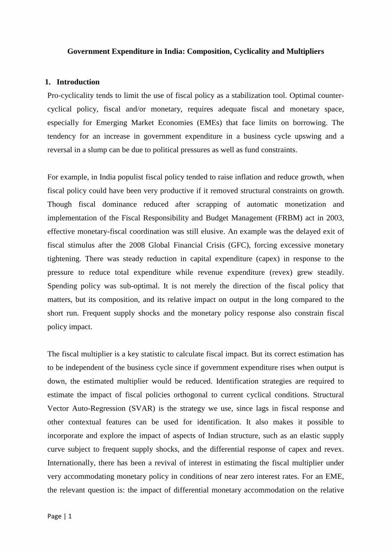
Figure 1: Revenue and capital expenditure

Figure 1 shows revenue expenditure has dominated total Government expenditure (totex) in

India and increased steadily compared to capital expenditure, which shows a flatter trend over

time, with significant increases being followed by decreases of equal or even greater

magnitude, implying sharp fluctuations around the mean. These sharp fluctuations in capital

expenditure growth rates manifest in a large variance of the series.

Despite a slight upward shift in the capital expenditure series since 2011, the gap between

real revenue expenditure and real capital expenditure has widened, especially since 2005

(Figure 1). Since the introduction of FRBM in 2003, fiscal authorities are under pressure to

keep the fiscal balance in check. Central Government’s total expenditure fell from 16% to

14% of GDP in the 2 years following implementation of FRBM. However, the brunt of this

expenditure control was borne by capital expenditure which declined to 1.8% of the GDP in

2008-09 from 6.2% in the 1980s while revenue expenditure continued to show a rising trend

0

200

400

600

800

1000

1200

1400

19

98

Q1

19

98

Q4

19

99

Q3

20

00

Q2

20

01

Q1

20

01

Q4

20

02

Q3

20

03

Q2

20

04

Q1

20

04

Q4

20

05

Q3

20

06

Q2

20

07

Q1

20

07

Q4

20

08

Q3

20

09

Q2

20

10

Q1

20

10

Q4

20

11

Q3

20

12

Q2

20

13

Q1

20

13

Q4

Revenue Expenditure (Real) Capital Expenditure (Real)

Page | 10

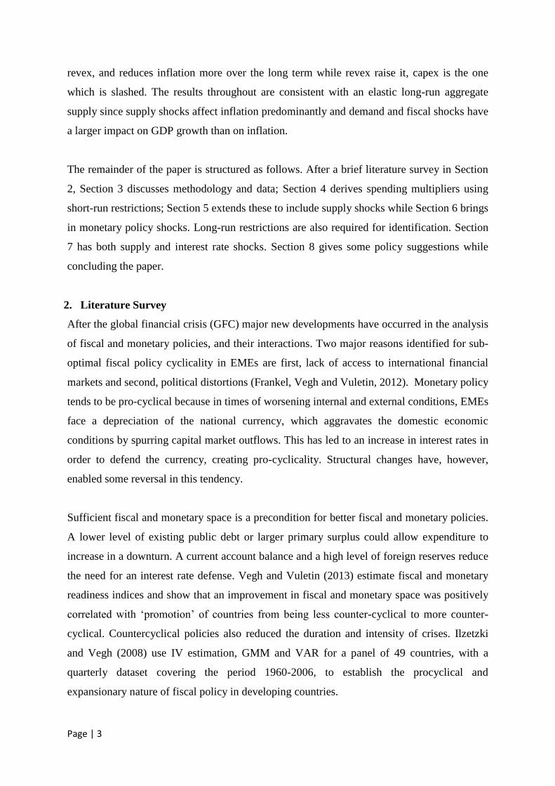
throughout1. Figure 2 shows the fluctuations and stagnation in GDP growth rate this may

have been responsible for.

Figure 2: GDP growth rate

We use quarterly data on total, revenue and capital expenditure, retrieved from the monthly

accounts available on the website of the Controller General of India (http://www.cga.nic.in/),

Gross Domestic Product (GDP) at constant prices (available at dbie.rbi.org.in), for the period

1998-Q1 to 2014Q3. In order to estimate the long run supply curve for India for the same

period and frequency, we use the quarterly average of the monthly wholesale price index

(WPI) series (at 1993-94 base year) and the quarterly GDP series. In order to control for

monetary policy stance, quarterly averages of call money market rates (CMMR) have been

used (Source: dbie.rbi.org.in). To account for business cycle fluctuations, a traditional

measure of output gap, the cyclical component of real GDP, is obtained using the Hodrick-

Prescott Filter. Annual data for GDP, WPI and total, revenue and capital expenditure is

sourced from Database for Indian Economy, RBI.

The data on GDP and fiscal variables have been de-seasonalised using the X-12 technique of

the Census Bureau of USA and converted into logarithms. All of these variables, converted

into growth rates, were stationary at 5% level of significance using the Augmented Dickey

Fuller (ADF) test. The output gap and WPI inflation rate series are stationary, using ADF

test, at both 5% and 1% levels of significance.

CMMR is stationary at 10% level of significance. We also define the real interest rate

variable as the difference between the short term nominal interest rate and expected inflation

1 Following the Sixth Pay Commission, wages and salaries of government employees increased along with

subsidies and interest payments on account of higher fiscal deficit.

0

5

10

15

19

99

Q1

19

99

Q3

20

00

Q1

20

00

Q3

20

01

Q1

20

01

Q3

20

02

Q1

20

02

Q3

20

03

Q1

20

03

Q3

20

04

Q1

20

04

Q3

20

05

Q1

20

05

Q3

20

06

Q1

20

06

Q3

20

07

Q1

20

07

Q3

20

08

Q1

20

08

Q3

20

09

Q1

20

09

Q3

20

10

Q1

20

10

Q3

20

11

Q1

20

11

Q3

20

12

Q1

20

12

Q3

20

13

Q1

20

13

Q3

20

14

Q1

GDP Growth Rate

Page | 11

rate. Because of larger scale data dissemination in India now, it is easier for individuals and

firms to have information to build up current expectations regarding future inflation rate. We

assume expectations are realized, therefore:

Where,

3.3 Analysis of cyclicality of expenditure policy

Following Vegh and Vuletin (2013), the measure of fiscal policy cyclicality is estimated by

the correlation of cyclical component of real total general government expenditure and the

cyclical component of real GDP, both computed using the Hodrick-Prescott filter.

( )

( )

Where

A negative correlation coefficient amounts to counter-cyclical fiscal policy, with the

Government Expenditure increasing during a downturn in the business cycle, considered to

be an optimal policy stance. However, in order to pursue counter-cyclical fiscal/monetary

policy, there should be enough fiscal and monetary space. Policy readiness indices give an

indication of such space.

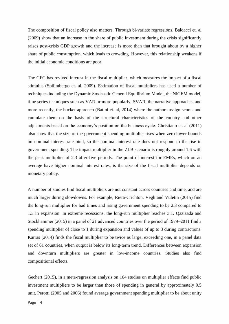
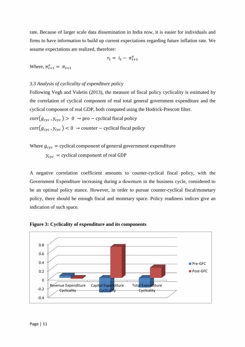
Figure 3: Cyclicality of expenditure and its components

-0.4

-0.2

0

0.2

0.4

0.6

0.8

Revenue ExpenditureCyclicality

Capital ExpenditureCyclicality

Total ExpenditureCyclicality

Pre-GFC

Post-GFC

Page | 12

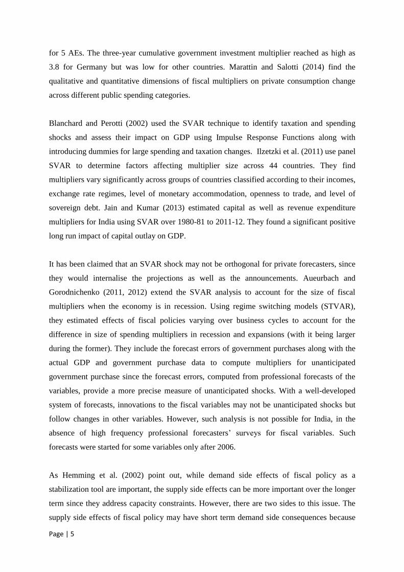
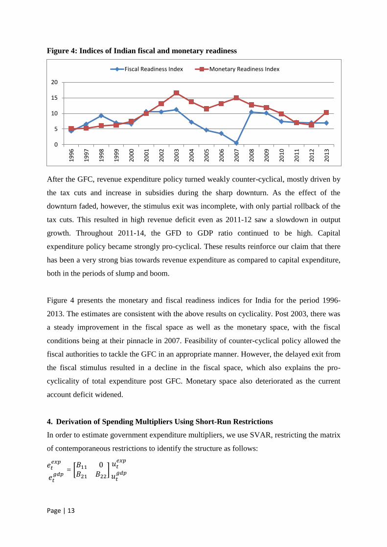
Fiscal Readiness Index is defined as the sum of two components- (i) Fiscal deficit as a

percentage of GDP and (ii) External debt (both private as well as public) as a percentage of

GDP. Both indicators are normalized on a scale of 0 to 10 and therefore, the overall fiscal

readiness index is measured on a scale of 0 to 20 with 0 being the highest level of readiness

and 20 the lowest. A lower level of existing public debt or larger primary surplus would also

keep the debt servicing costs in check and the authorities could comfortably increase

expenditure in the face of a downturn.

Monetary Readiness Index is defined as the sum of two components- (i) Foreign Reserves as

a percentage of GDP and (ii) Current Account Balance as a percentage of GDP – both

normalized on a scale of 0 to 10. The overall monetary readiness index is measured on a scale

of 0 (lowest monetary readiness) to 20 (highest monetary readiness). High level of foreign

reserves and Current Account Balance will ensure that the monetary authorities in EMEs do

not have to increase interest rates during slumps in order to avoid capital outflows.

To distinguish between the response of Central Government revex and capex in the business

cycle, we compute cyclical components of both expenditure heads as well as total central

government expenditure. Figure 3 displays the results of the analysis. Before the GFC, total

government expenditure was counter-cyclical. This result probably holds because of the

reduction in total expenditure that was carried out after the implementation of FRBM in

2003-04, coinciding with a boom. Post the GFC, the total expenditure policy of the Central

Government became pro-cyclical, since the rollback of the post GFC fiscal stimulus was

delayed.

However, separate analysis of capital and revenue expenditure brings out finer details. Figure

3 shows that before the GFC hit the global economy, India had a pro-cyclical revenue

expenditure and counter-cyclical capital expenditure policy. This is not so surprising, given

post the implementation of FRBM, capital expenditure as a percentage of GDP declined

sharply as compared to the average 1980s level, while revenue expenditure grew to 15% in

the same period from 11.2% in the 1980s. The counter-cyclicality of total expenditure

manifested in a decrease in capacity-building investments during the period of output growth.

Page | 13

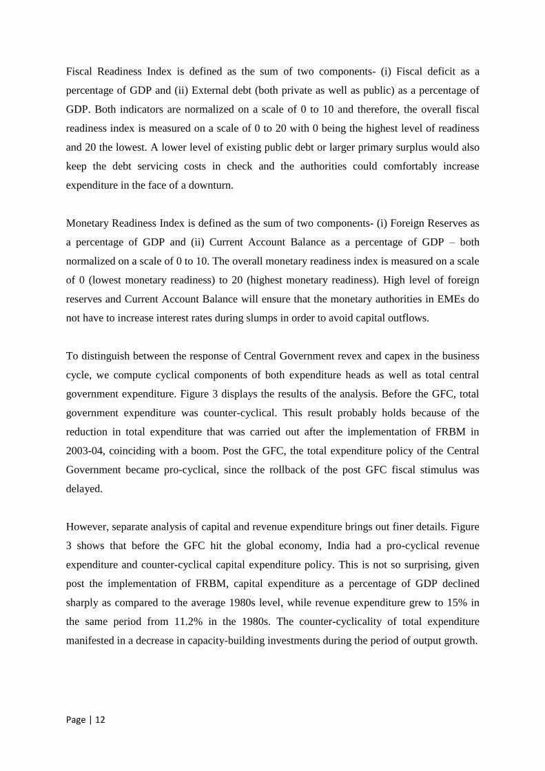
Figure 4: Indices of Indian fiscal and monetary readiness

After the GFC, revenue expenditure policy turned weakly counter-cyclical, mostly driven by

the tax cuts and increase in subsidies during the sharp downturn. As the effect of the

downturn faded, however, the stimulus exit was incomplete, with only partial rollback of the

tax cuts. This resulted in high revenue deficit even as 2011-12 saw a slowdown in output

growth. Throughout 2011-14, the GFD to GDP ratio continued to be high. Capital

expenditure policy became strongly pro-cyclical. These results reinforce our claim that there

has been a very strong bias towards revenue expenditure as compared to capital expenditure,

both in the periods of slump and boom.

Figure 4 presents the monetary and fiscal readiness indices for India for the period 1996-

2013. The estimates are consistent with the above results on cyclicality. Post 2003, there was

a steady improvement in the fiscal space as well as the monetary space, with the fiscal

conditions being at their pinnacle in 2007. Feasibility of counter-cyclical policy allowed the

fiscal authorities to tackle the GFC in an appropriate manner. However, the delayed exit from

the fiscal stimulus resulted in a decline in the fiscal space, which also explains the pro-

cyclicality of total expenditure post GFC. Monetary space also deteriorated as the current

account deficit widened.

4. Derivation of Spending Multipliers Using Short-Run Restrictions

In order to estimate government expenditure multipliers, we use SVAR, restricting the matrix

of contemporaneous restrictions to identify the structure as follows:

= [

]

0

5

10

15

20

19

96

19

97

19

98

19

99

20

00

20

01

20

02

20

03

20

04

20

05

20

06

20

07

20

08

20

09

20

10

20

11

20

12

20

13

Fiscal Readiness Index Monetary Readiness Index

Page | 14

Where the LHS represents vector of reduced form shocks and the ut vector represents the

structural shocks. B is the matrix of contemporaneous coefficients. The restriction implies the

spending variables will impact output in the short run but not vice-a-versa. Fiscal decision

and implementation lags justify such as identification.

The ratio of impulse responses of output to fiscal variables and of fiscal to fiscal variables

gives the elasticity, which when divided by a historical average ratio of real spending to GDP

gives the multiplier. That is, the sample mean of output to spending ratio is multiplied by the

ratio of impulse response of output growth to structural spending shock and impulse response

of spending growth to structural spending shock.

=

Where,

( )

( )

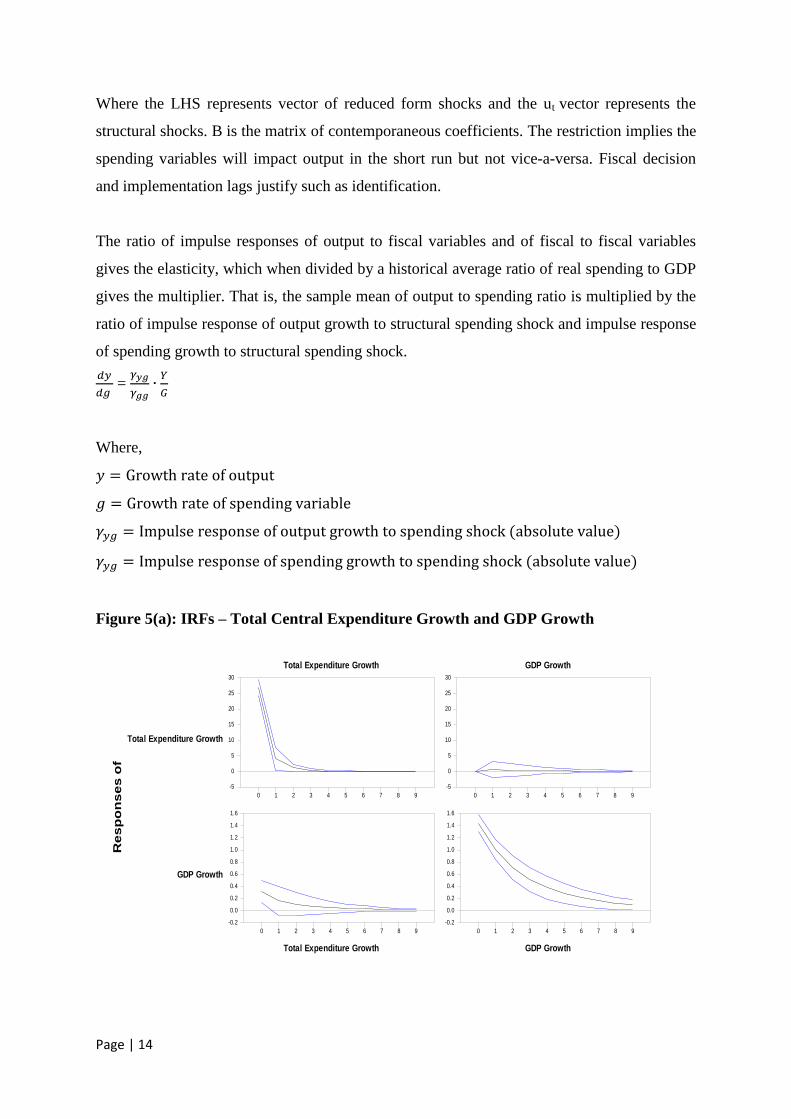
Figure 5(a): IRFs – Total Central Expenditure Growth and GDP Growth

Re

sp

on

se

s o

f

Total Expenditure Growth

GDP Growth

Total Expenditure Growth

Total Expenditure Growth

GDP Growth

GDP Growth

0 1 2 3 4 5 6 7 8 9

-5

0

5

10

15

20

25

30

0 1 2 3 4 5 6 7 8 9

-5

0

5

10

15

20

25

30

0 1 2 3 4 5 6 7 8 9

-0.2

0.0

0.2

0.4

0.6

0.8

1.0

1.2

1.4

1.6

0 1 2 3 4 5 6 7 8 9

-0.2

0.0

0.2

0.4

0.6

0.8

1.0

1.2

1.4

1.6

Page | 15

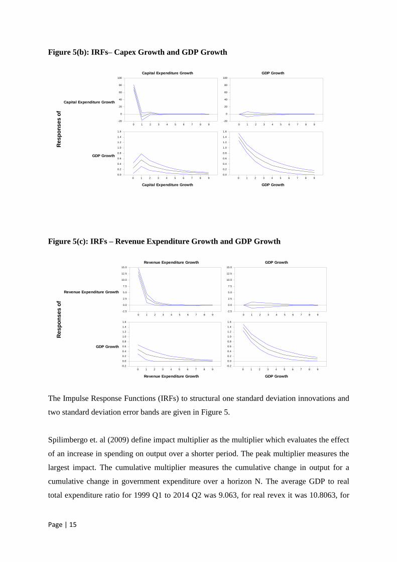
Figure 5(b): IRFs– Capex Growth and GDP Growth

Figure 5(c): IRFs – Revenue Expenditure Growth and GDP Growth

The Impulse Response Functions (IRFs) to structural one standard deviation innovations and

two standard deviation error bands are given in Figure 5.

Spilimbergo et. al (2009) define impact multiplier as the multiplier which evaluates the effect

of an increase in spending on output over a shorter period. The peak multiplier measures the

largest impact. The cumulative multiplier measures the cumulative change in output for a

cumulative change in government expenditure over a horizon N. The average GDP to real

total expenditure ratio for 1999 Q1 to 2014 Q2 was 9.063, for real revex it was 10.8063, for

Re

sp

on

se

s o

f

Capital Expenditure Growth

GDP Growth

Capital Expenditure Growth

Capital Expenditure Growth

GDP Growth

GDP Growth

0 1 2 3 4 5 6 7 8 9

-20

0

20

40

60

80

100

0 1 2 3 4 5 6 7 8 9

-20

0

20

40

60

80

100

0 1 2 3 4 5 6 7 8 9

0.0

0.2

0.4

0.6

0.8

1.0

1.2

1.4

1.6

0 1 2 3 4 5 6 7 8 9

0.0

0.2

0.4

0.6

0.8

1.0

1.2

1.4

1.6

Re

sp

on

se

s o

f

Revenue Expenditure Growth

GDP Growth

Revenue Expenditure Growth

Revenue Expenditure Growth

GDP Growth

GDP Growth

0 1 2 3 4 5 6 7 8 9

-2.5

0.0

2.5

5.0

7.5

10.0

12.5

15.0

0 1 2 3 4 5 6 7 8 9

-2.5

0.0

2.5

5.0

7.5

10.0

12.5

15.0

0 1 2 3 4 5 6 7 8 9

-0.2

0.0

0.2

0.4

0.6

0.8

1.0

1.2

1.4

1.6

0 1 2 3 4 5 6 7 8 9

-0.2

0.0

0.2

0.4

0.6

0.8

1.0

1.2

1.4

1.6

Page | 16

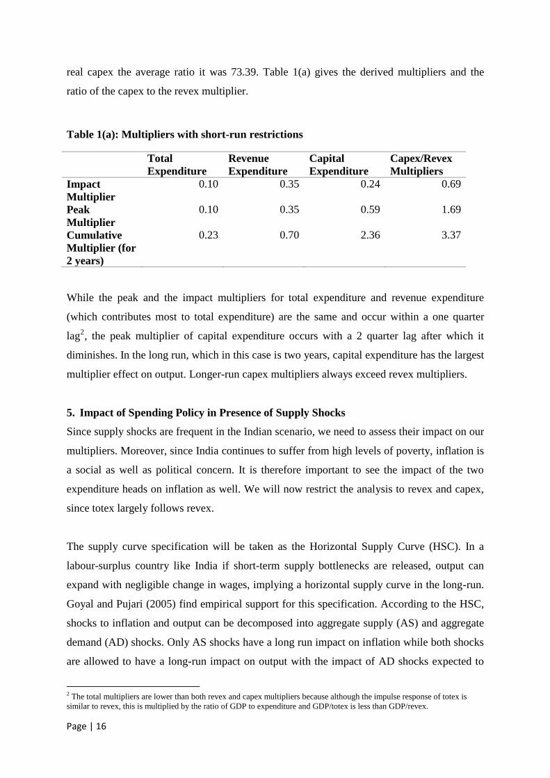
real capex the average ratio it was 73.39. Table 1(a) gives the derived multipliers and the

ratio of the capex to the revex multiplier.

Table 1(a): Multipliers with short-run restrictions

Total

Expenditure

Revenue

Expenditure

Capital

Expenditure

Capex/Revex

Multipliers

Impact

Multiplier

0.10 0.35 0.24 0.69

Peak

Multiplier

0.10 0.35 0.59 1.69

Cumulative

Multiplier (for

2 years)

0.23 0.70 2.36 3.37

While the peak and the impact multipliers for total expenditure and revenue expenditure

(which contributes most to total expenditure) are the same and occur within a one quarter

lag2, the peak multiplier of capital expenditure occurs with a 2 quarter lag after which it

diminishes. In the long run, which in this case is two years, capital expenditure has the largest

multiplier effect on output. Longer-run capex multipliers always exceed revex multipliers.

5. Impact of Spending Policy in Presence of Supply Shocks

Since supply shocks are frequent in the Indian scenario, we need to assess their impact on our

multipliers. Moreover, since India continues to suffer from high levels of poverty, inflation is

a social as well as political concern. It is therefore important to see the impact of the two

expenditure heads on inflation as well. We will now restrict the analysis to revex and capex,

since totex largely follows revex.

The supply curve specification will be taken as the Horizontal Supply Curve (HSC). In a

labour-surplus country like India if short-term supply bottlenecks are released, output can

expand with negligible change in wages, implying a horizontal supply curve in the long-run.

Goyal and Pujari (2005) find empirical support for this specification. According to the HSC,

shocks to inflation and output can be decomposed into aggregate supply (AS) and aggregate

demand (AD) shocks. Only AS shocks have a long run impact on inflation while both shocks

are allowed to have a long-run impact on output with the impact of AD shocks expected to

2 The total multipliers are lower than both revex and capex multipliers because although the impulse response of totex is

similar to revex, this is multiplied by the ratio of GDP to expenditure and GDP/totex is less than GDP/revex.

Page | 17

dominate. The structural moving average representation of system in 3-variable VAR cases

is:

= [

] [

]

The long-run restrictions used here imply that inflation is mainly determined through supply

shocks ( ) and that demand shocks ( ) have no impact on inflation in the long run.

Output growth rate in the long-run is determined by supply, demand ( ) and fiscal

shocks( ). For both revenue and capital expenditure, we allow all the three shocks to have

a long-run impact on the grounds that long-run spending decisions incorporate the various

demand and supply shocks in order to cushion the economy from such shocks in the long-run.

Although political economy considerations dominate fiscal policy decisions, the welfare loss

from failing to account for large negative shocks in the spending decision may materialise in

a loss of political power.

Apart from the two long-run restrictions given above, one more restriction is needed. We

therefore, use our earlier short-run restriction and restrict the contemporaneous coefficient

matrix as below:

= [

] [

]

The above specification allows for a positively sloped short run aggregate supply curve. That

is, both demand and supply shocks affect inflation and output growth rate in the short-run

when constraints hold. But since bottlenecks affect prices at every output level and shift up

the curve, the AS curve may be elastic even in the short-run, although subject to volatile

shocks. These shocks would impact short run prices and output more strongly than in the

long-run. Furthermore, we have allowed for the spending variables to have a short-run impact

on inflation. While an increase in revenue expenditure because of the increase in wages and

salaries of government employees might lead to increase in demand of goods and services,

spurring a price increase, an increase in capital outlay, even though directed at eliminating the

Page | 18

structural bottlenecks precluding long-run output growth, may increase the price levels in the

short-run by increasing demand for labour as well as capital, required to complete large-scale

projects.

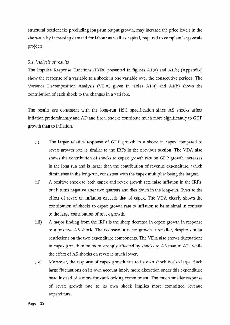
5.1 Analysis of results

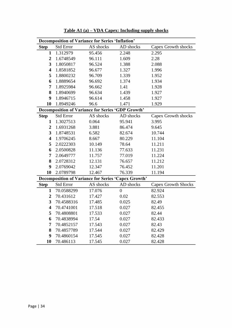
The Impulse Response Functions (IRFs) presented in figures A1(a) and A1(b) (Appendix)

show the response of a variable to a shock in one variable over the consecutive periods. The

Variance Decomposition Analysis (VDA) given in tables A1(a) and A1(b) shows the

contribution of each shock to the changes in a variable.

The results are consistent with the long-run HSC specification since AS shocks affect

inflation predominantly and AD and fiscal shocks contribute much more significantly to GDP

growth than to inflation.

(i) The larger relative response of GDP growth to a shock in capex compared to

revex growth rate is similar to the IRFs in the previous section. The VDA also

shows the contribution of shocks to capex growth rate on GDP growth increases

in the long run and is larger than the contribution of revenue expenditure, which

diminishes in the long-run, consistent with the capex multiplier being the largest.

(ii) A positive shock to both capex and revex growth rate raise inflation in the IRFs,

but it turns negative after two quarters and dies down in the long-run. Even so the

effect of revex on inflation exceeds that of capex. The VDA clearly shows the

contribution of shocks to capex growth rate to inflation to be minimal in contrast

to the large contribution of revex growth.

(iii) A major finding from the IRFs is the sharp decrease in capex growth in response

to a positive AS shock. The decrease in revex growth is smaller, despite similar

restrictions on the two expenditure components. The VDA also shows fluctuations

in capex growth to be more strongly affected by shocks to AS than to AD, while

the effect of AS shocks on revex is much lower.

(iv) Moreover, the response of capex growth rate to its own shock is also large. Such

large fluctuations on its own account imply more discretion under this expenditure

head instead of a more forward-looking commitment. The much smaller response

of revex growth rate to its own shock implies more committed revenue

expenditure.

Page | 19

In presence of a sudden inflation spike, wages and salaries of government workers are

difficult to reduce and subsidies increase because of a ‘pandering’ effect. Since there is a

pressure to keep the fiscal balances in check, it is easier to reduce an element of spending less

visible (at least in the short-run) to the public eye. Figure 1 shows the declining ratio of

capital to revenue expenditure that can therefore be expected under frequent supply shocks.

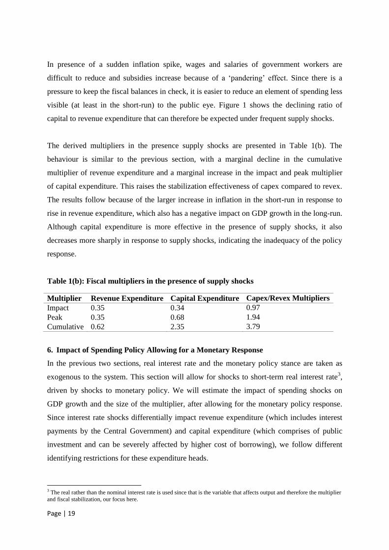
The derived multipliers in the presence supply shocks are presented in Table 1(b). The

behaviour is similar to the previous section, with a marginal decline in the cumulative

multiplier of revenue expenditure and a marginal increase in the impact and peak multiplier

of capital expenditure. This raises the stabilization effectiveness of capex compared to revex.

The results follow because of the larger increase in inflation in the short-run in response to

rise in revenue expenditure, which also has a negative impact on GDP growth in the long-run.

Although capital expenditure is more effective in the presence of supply shocks, it also

decreases more sharply in response to supply shocks, indicating the inadequacy of the policy

response.

Table 1(b): Fiscal multipliers in the presence of supply shocks

Multiplier Revenue Expenditure Capital Expenditure Capex/Revex Multipliers

Impact 0.35 0.34 0.97

Peak 0.35 0.68 1.94

Cumulative 0.62 2.35 3.79

6. Impact of Spending Policy Allowing for a Monetary Response

In the previous two sections, real interest rate and the monetary policy stance are taken as

exogenous to the system. This section will allow for shocks to short-term real interest rate3,

driven by shocks to monetary policy. We will estimate the impact of spending shocks on

GDP growth and the size of the multiplier, after allowing for the monetary policy response.

Since interest rate shocks differentially impact revenue expenditure (which includes interest

payments by the Central Government) and capital expenditure (which comprises of public

investment and can be severely affected by higher cost of borrowing), we follow different

identifying restrictions for these expenditure heads.

3 The real rather than the nominal interest rate is used since that is the variable that affects output and therefore the multiplier

and fiscal stabilization, our focus here.

Page | 20

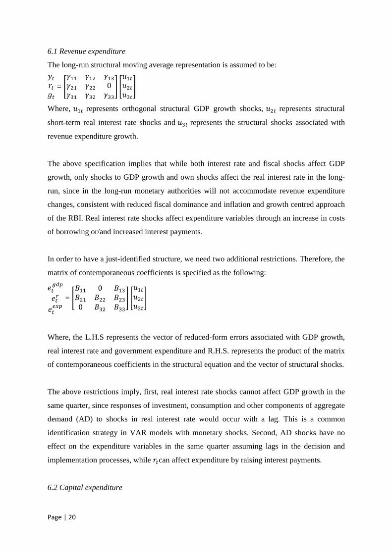
6.1 Revenue expenditure

The long-run structural moving average representation is assumed to be:

= [

] [

]

Where, represents orthogonal structural GDP growth shocks, represents structural

short-term real interest rate shocks and represents the structural shocks associated with

revenue expenditure growth.

The above specification implies that while both interest rate and fiscal shocks affect GDP

growth, only shocks to GDP growth and own shocks affect the real interest rate in the long-

run, since in the long-run monetary authorities will not accommodate revenue expenditure

changes, consistent with reduced fiscal dominance and inflation and growth centred approach

of the RBI. Real interest rate shocks affect expenditure variables through an increase in costs

of borrowing or/and increased interest payments.

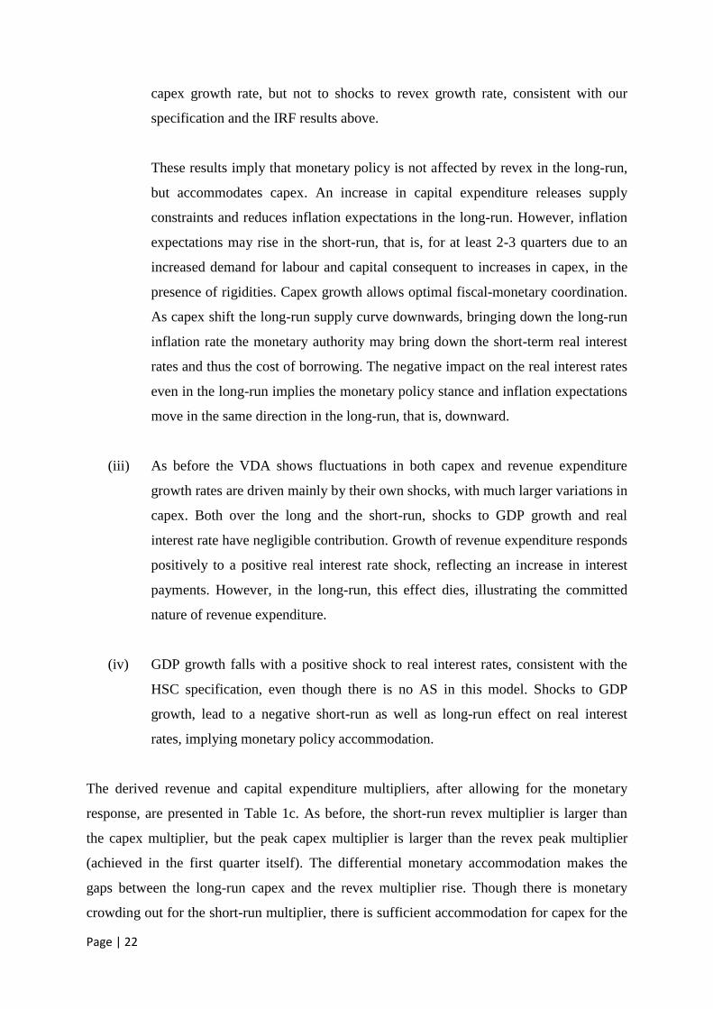
In order to have a just-identified structure, we need two additional restrictions. Therefore, the

matrix of contemporaneous coefficients is specified as the following:

= [

] [

]

Where, the L.H.S represents the vector of reduced-form errors associated with GDP growth,

real interest rate and government expenditure and R.H.S. represents the product of the matrix

of contemporaneous coefficients in the structural equation and the vector of structural shocks.

The above restrictions imply, first, real interest rate shocks cannot affect GDP growth in the

same quarter, since responses of investment, consumption and other components of aggregate

demand (AD) to shocks in real interest rate would occur with a lag. This is a common

identification strategy in VAR models with monetary shocks. Second, AD shocks have no

effect on the expenditure variables in the same quarter assuming lags in the decision and

implementation processes, while can affect expenditure by raising interest payments.

6.2 Capital expenditure

Page | 21

We assume , that is, shocks to growth in capex can have a long-run effect on real

interest rate. Real interest rates are affected by inflation expectations, which in turn are

affected by the growth of capital expenditure. Moreover, if the monetary authority observes

that the fiscal authority is directing resources towards unplugging the structural bottlenecks, it

might decrease the short-term interest rates. This eliminates the only possible restriction in

the SMA representation in the first case above.

In order to have a just-identified structure, we need three restrictions in the short-run matrix.

This fits in perfectly with the required theoretical restrictions on the contemporaneous

coefficients in this system.

= [

] [

]

In addition to restrictions specified for revenue expenditure, we assume on the

grounds that capital expenditure reacts to interest rate shocks with lags, as the cost of

borrowing increases, and not contemporaneously, unlike revenue expenditure.

6.3 Analysis of results

The IRFs presented in figures A2(a) and A2(b), and the VDA (Tables A2(a) and A2(b))

imply the following conclusions:

(i) The behaviour of GDP growth in response to a shock to capex growth is similar to

the response presented in the previous two sections, with capex having higher

long-run impact than revenue expenditure in the IRFs. The VDA also shows both

real interest rate shocks (monetary policy shocks) and capex growth shocks affect

GDP growth in the long-run, with the effect of capex increasing with time. In

contrast the effect of revex growth shocks on GDP growth decreases over time.

(ii) Shocks to capital expenditure growth have a negative impact on short-term real

interest rate both in the long-run as well as the short-run, unlike the negligible

impact of revenue expenditure, in the IRFs. The VDA shows real interest rate is

affected by shocks to GDP growth and is also significantly affected by shocks to

Page | 22

capex growth rate, but not to shocks to revex growth rate, consistent with our

specification and the IRF results above.

These results imply that monetary policy is not affected by revex in the long-run,

but accommodates capex. An increase in capital expenditure releases supply

constraints and reduces inflation expectations in the long-run. However, inflation

expectations may rise in the short-run, that is, for at least 2-3 quarters due to an

increased demand for labour and capital consequent to increases in capex, in the

presence of rigidities. Capex growth allows optimal fiscal-monetary coordination.

As capex shift the long-run supply curve downwards, bringing down the long-run

inflation rate the monetary authority may bring down the short-term real interest

rates and thus the cost of borrowing. The negative impact on the real interest rates

even in the long-run implies the monetary policy stance and inflation expectations

move in the same direction in the long-run, that is, downward.

(iii) As before the VDA shows fluctuations in both capex and revenue expenditure

growth rates are driven mainly by their own shocks, with much larger variations in

capex. Both over the long and the short-run, shocks to GDP growth and real

interest rate have negligible contribution. Growth of revenue expenditure responds

positively to a positive real interest rate shock, reflecting an increase in interest

payments. However, in the long-run, this effect dies, illustrating the committed

nature of revenue expenditure.

(iv) GDP growth falls with a positive shock to real interest rates, consistent with the

HSC specification, even though there is no AS in this model. Shocks to GDP

growth, lead to a negative short-run as well as long-run effect on real interest

rates, implying monetary policy accommodation.

The derived revenue and capital expenditure multipliers, after allowing for the monetary

response, are presented in Table 1c. As before, the short-run revex multiplier is larger than

the capex multiplier, but the peak capex multiplier is larger than the revex peak multiplier

(achieved in the first quarter itself). The differential monetary accommodation makes the

gaps between the long-run capex and the revex multiplier rise. Though there is monetary

crowding out for the short-run multiplier, there is sufficient accommodation for capex for the

Page | 23

long-run multiplier to be much larger. All other multipliers are smaller than those in Tables

1a and 1b, suggesting that Indian monetary policy enhances the long-run impact of capex, but

reduces that of every other multiplier.

Table 1c: Fiscal multipliers in the presence of a monetary response

Multiplier Revenue Expenditure Capital Expenditure Capex/Revex Multipliers

Impact 0.32 0.26 0.81

Peak 0.32 0.63 1.97

Cumulative 0.47 3.06 6.5

7. Impact of Spending Policy in Presence of Supply and Interest Rate Shocks

In this section, we extend our analysis to a 4-variable SVAR by including a short-term real

interest rate variable , as well as supply shocks. Structural shocks in the inflation equation

are AS shocks and structural shocks in the output growth equation are AD shocks. So the AD

shocks will now be separated from government spending and interest rate shocks. AD shocks

will include tax shocks, external sector shocks and other private sector investment and

consumption shocks. As before, the long-run and short-run coefficient matrices for analysis

of revex and capex differ. We continue with our earlier specification of a long-run HSC.

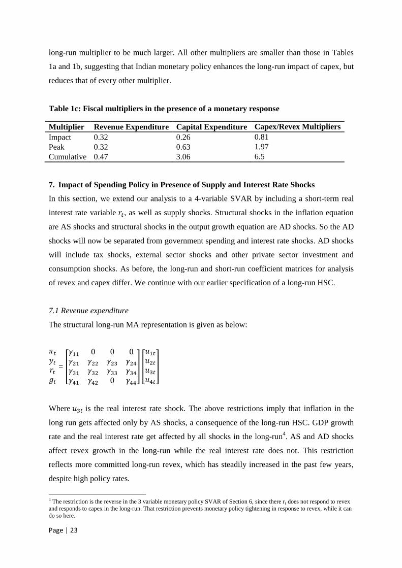
7.1 Revenue expenditure

The structural long-run MA representation is given as below:

= [

] [

]

Where is the real interest rate shock. The above restrictions imply that inflation in the

long run gets affected only by AS shocks, a consequence of the long-run HSC. GDP growth

rate and the real interest rate get affected by all shocks in the long-run4. AS and AD shocks

affect revex growth in the long-run while the real interest rate does not. This restriction

reflects more committed long-run revex, which has steadily increased in the past few years,

despite high policy rates.

4 The restriction is the reverse in the 3 variable monetary policy SVAR of Section 6, since there rt does not respond to revex

and responds to capex in the long-run. That restriction prevents monetary policy tightening in response to revex, while it can

do so here.

Page | 24

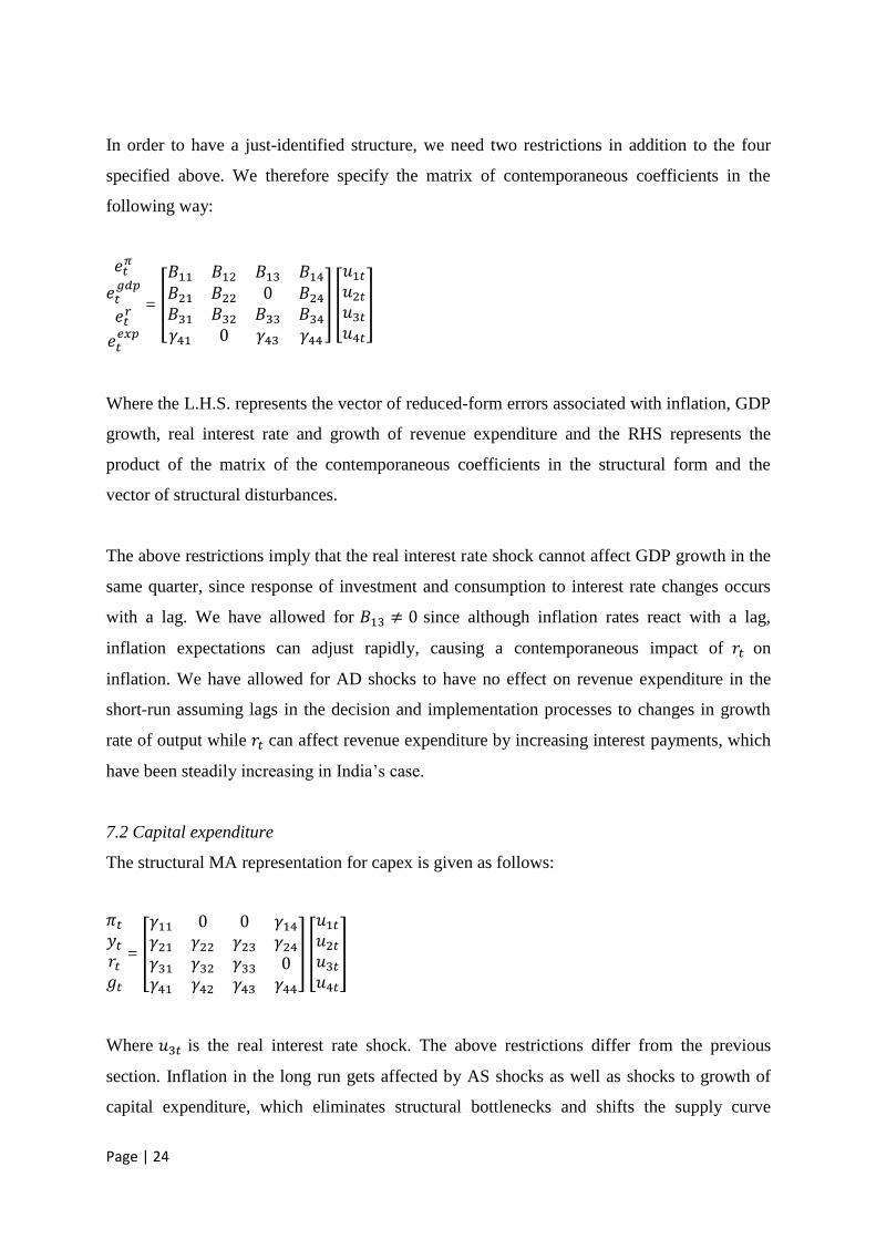
In order to have a just-identified structure, we need two restrictions in addition to the four

specified above. We therefore specify the matrix of contemporaneous coefficients in the

following way:

= [

] [

]

Where the L.H.S. represents the vector of reduced-form errors associated with inflation, GDP

growth, real interest rate and growth of revenue expenditure and the RHS represents the

product of the matrix of the contemporaneous coefficients in the structural form and the

vector of structural disturbances.

The above restrictions imply that the real interest rate shock cannot affect GDP growth in the

same quarter, since response of investment and consumption to interest rate changes occurs

with a lag. We have allowed for since although inflation rates react with a lag,

inflation expectations can adjust rapidly, causing a contemporaneous impact of on

inflation. We have allowed for AD shocks to have no effect on revenue expenditure in the

short-run assuming lags in the decision and implementation processes to changes in growth

rate of output while can affect revenue expenditure by increasing interest payments, which

have been steadily increasing in India’s case.

7.2 Capital expenditure

The structural MA representation for capex is given as follows:

= [

] [

]

Where is the real interest rate shock. The above restrictions differ from the previous

section. Inflation in the long run gets affected by AS shocks as well as shocks to growth of

capital expenditure, which eliminates structural bottlenecks and shifts the supply curve

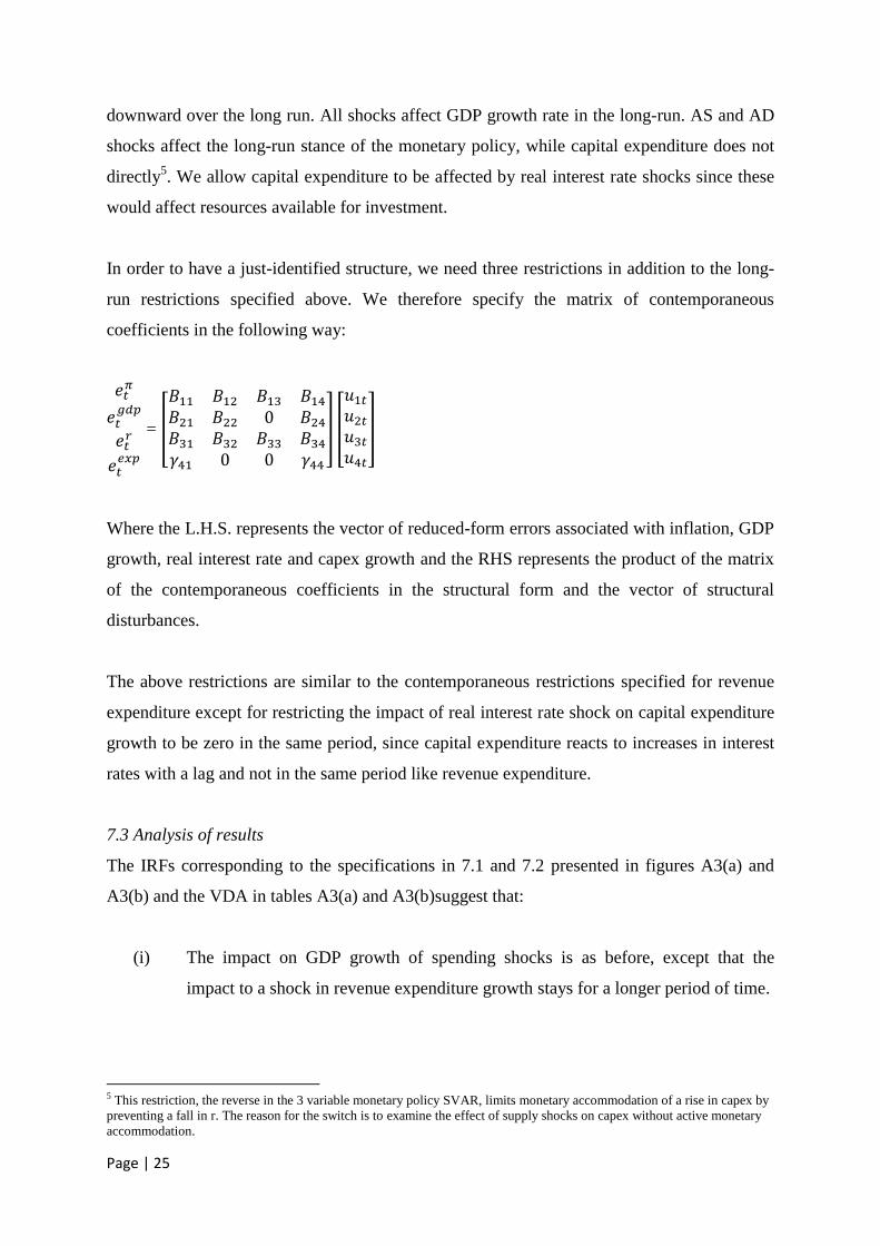
Page | 25

downward over the long run. All shocks affect GDP growth rate in the long-run. AS and AD

shocks affect the long-run stance of the monetary policy, while capital expenditure does not

directly5. We allow capital expenditure to be affected by real interest rate shocks since these

would affect resources available for investment.

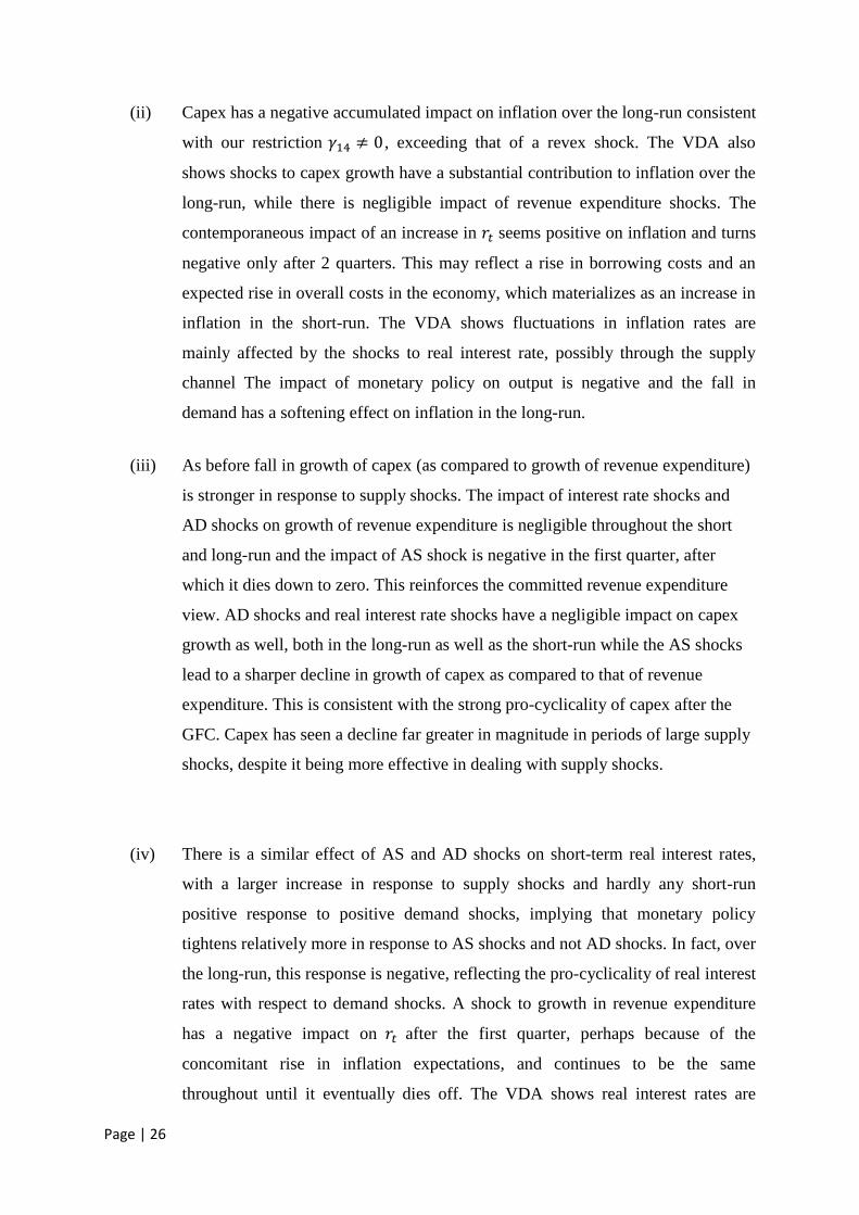
In order to have a just-identified structure, we need three restrictions in addition to the long-

run restrictions specified above. We therefore specify the matrix of contemporaneous

coefficients in the following way:

= [

] [

]

Where the L.H.S. represents the vector of reduced-form errors associated with inflation, GDP

growth, real interest rate and capex growth and the RHS represents the product of the matrix

of the contemporaneous coefficients in the structural form and the vector of structural

disturbances.

The above restrictions are similar to the contemporaneous restrictions specified for revenue

expenditure except for restricting the impact of real interest rate shock on capital expenditure

growth to be zero in the same period, since capital expenditure reacts to increases in interest

rates with a lag and not in the same period like revenue expenditure.

7.3 Analysis of results

The IRFs corresponding to the specifications in 7.1 and 7.2 presented in figures A3(a) and

A3(b) and the VDA in tables A3(a) and A3(b)suggest that:

(i) The impact on GDP growth of spending shocks is as before, except that the

impact to a shock in revenue expenditure growth stays for a longer period of time.

5 This restriction, the reverse in the 3 variable monetary policy SVAR, limits monetary accommodation of a rise in capex by

preventing a fall in r. The reason for the switch is to examine the effect of supply shocks on capex without active monetary

accommodation.

Page | 26

(ii) Capex has a negative accumulated impact on inflation over the long-run consistent

with our restriction , exceeding that of a revex shock. The VDA also

shows shocks to capex growth have a substantial contribution to inflation over the

long-run, while there is negligible impact of revenue expenditure shocks. The

contemporaneous impact of an increase in seems positive on inflation and turns

negative only after 2 quarters. This may reflect a rise in borrowing costs and an

expected rise in overall costs in the economy, which materializes as an increase in

inflation in the short-run. The VDA shows fluctuations in inflation rates are

mainly affected by the shocks to real interest rate, possibly through the supply

channel The impact of monetary policy on output is negative and the fall in

demand has a softening effect on inflation in the long-run.

(iii) As before fall in growth of capex (as compared to growth of revenue expenditure)

is stronger in response to supply shocks. The impact of interest rate shocks and

AD shocks on growth of revenue expenditure is negligible throughout the short

and long-run and the impact of AS shock is negative in the first quarter, after

which it dies down to zero. This reinforces the committed revenue expenditure

view. AD shocks and real interest rate shocks have a negligible impact on capex

growth as well, both in the long-run as well as the short-run while the AS shocks

lead to a sharper decline in growth of capex as compared to that of revenue

expenditure. This is consistent with the strong pro-cyclicality of capex after the

GFC. Capex has seen a decline far greater in magnitude in periods of large supply

shocks, despite it being more effective in dealing with supply shocks.

(iv) There is a similar effect of AS and AD shocks on short-term real interest rates,

with a larger increase in response to supply shocks and hardly any short-run

positive response to positive demand shocks, implying that monetary policy

tightens relatively more in response to AS shocks and not AD shocks. In fact, over

the long-run, this response is negative, reflecting the pro-cyclicality of real interest

rates with respect to demand shocks. A shock to growth in revenue expenditure

has a negative impact on after the first quarter, perhaps because of the

concomitant rise in inflation expectations, and continues to be the same

throughout until it eventually dies off. The VDA shows real interest rates are

Page | 27

mainly affected by shocks to inflation rates with negligible contribution of

revenue expenditure growth. Shocks to capex growth do have a significant

contribution to real interest rates, which may be due to inadequate monetary

response to falling inflation expectations as capex grows6. The contemporaneous

impact of real interest rate to shocks in capex growth is positive, it turns negative

and stays so over the long run as the Central Bank accommodates reduction in

structural constraints. The positive contemporaneous impact may be because

capex is rising when supply shocks are absent and inflation expectations are

falling. Since the CB tightens in response to an AS shock, when capex also falls

sharply, covariance is high for the two variables. The fact that monetary tightening

accompanies a decline in public capital expenditure implies an aggravation of

supply shocks.

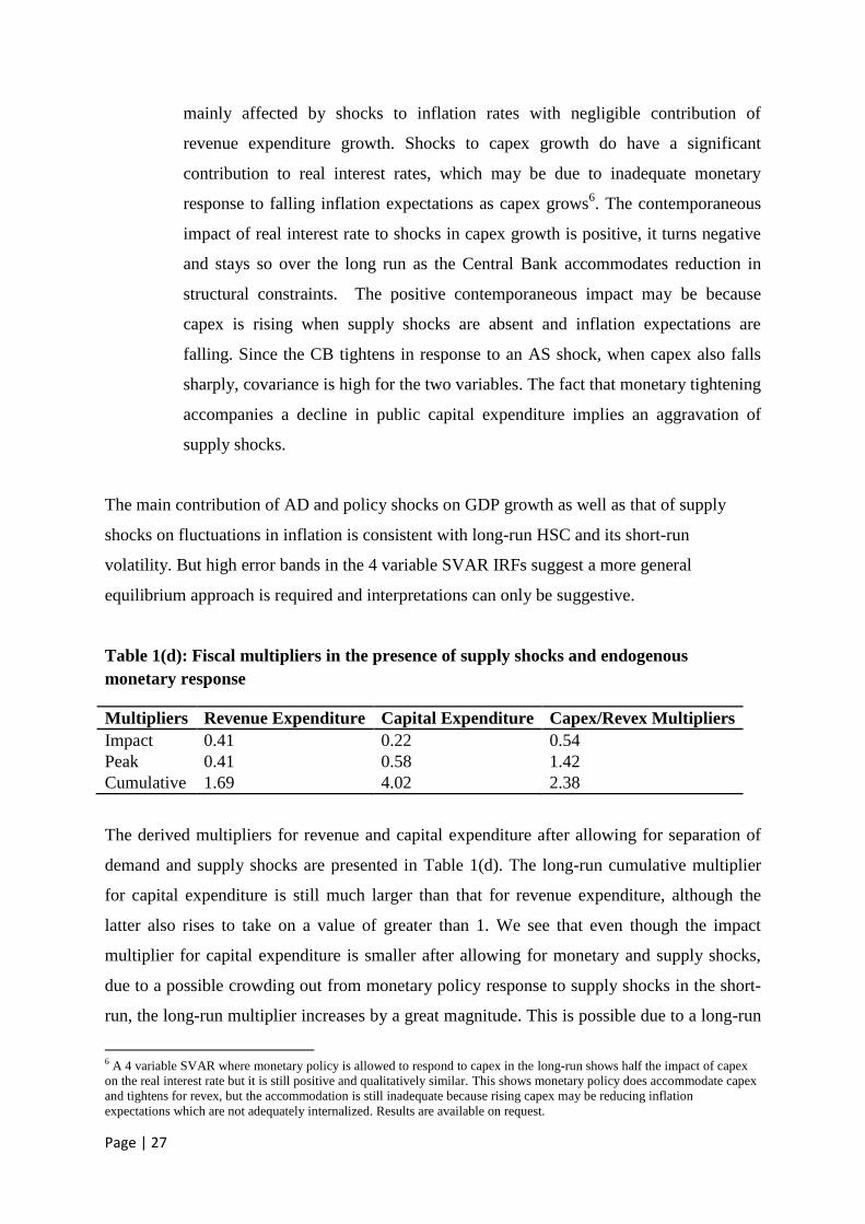
The main contribution of AD and policy shocks on GDP growth as well as that of supply

shocks on fluctuations in inflation is consistent with long-run HSC and its short-run

volatility. But high error bands in the 4 variable SVAR IRFs suggest a more general

equilibrium approach is required and interpretations can only be suggestive.

Table 1(d): Fiscal multipliers in the presence of supply shocks and endogenous

monetary response

Multipliers Revenue Expenditure Capital Expenditure Capex/Revex Multipliers

Impact 0.41 0.22 0.54

Peak 0.41 0.58 1.42

Cumulative 1.69 4.02 2.38

The derived multipliers for revenue and capital expenditure after allowing for separation of

demand and supply shocks are presented in Table 1(d). The long-run cumulative multiplier

for capital expenditure is still much larger than that for revenue expenditure, although the

latter also rises to take on a value of greater than 1. We see that even though the impact

multiplier for capital expenditure is smaller after allowing for monetary and supply shocks,

due to a possible crowding out from monetary policy response to supply shocks in the short-

run, the long-run multiplier increases by a great magnitude. This is possible due to a long-run

6 A 4 variable SVAR where monetary policy is allowed to respond to capex in the long-run shows half the impact of capex

on the real interest rate but it is still positive and qualitatively similar. This shows monetary policy does accommodate capex

and tightens for revex, but the accommodation is still inadequate because rising capex may be reducing inflation

expectations which are not adequately internalized. Results are available on request.

Page | 28

monetary accommodation in the form of lower interest rates as well as lower inflation in the

long-run.

8. Policy Suggestions and Conclusion

While the Indian Government received accolades for substantially reducing its fiscal deficit,

the short-sighted approach towards expenditure composition was less obvious. The bias

towards short-termism materialized in a sharp decrease in capital expenditure over the 2003-

2007 ‘boom’ period. Deficit reduction increased fiscal policy space for response to the GFC

and also boosted confidence of financial markets. But the economy bore the brunt of reduced

capex post 2008, in the form of a stagnating GDP growth rate.

Our results support the above claim. Capital expenditure not only has a much larger long-run

positive impact on output, compared to revenue expenditure, but it also has a smaller short-

run impact on inflation and reduces inflation volatility, since it eliminates structural

bottlenecks. An increase in capital expenditure also has a negative impact on short-run real

interest rate, as monetary authorities accommodate capacity-building initiatives of the

government. In contrast, an increase in revenue expenditure has a strong short-run positive

impact on real interest rate. The results suggest evaluation of spending policy in India should

be disaggregated, since analysis of total expenditure gives an incomplete picture of the fiscal

impulse.

The impact of macroeconomic variables on revenue expenditure is low since it is strongly

committed due to political factors. Revenue expenditure is thought to have larger short-run

benefits since it contributes to re-election. However, capital expenditure shows greater impact

on GDP growth within 2 years, that is, within the electoral cycle. The government, therefore,

should have strong incentives to push up capex. Sharper decrease in capital compared to

revenue expenditure in response to supply shocks is short-sighted. Decisions have not been

optimal.

Government capex can also, however, be poorly designed and wasteful. Devarajan et. al

(1996) show in an endogenous growth model, that if the share of capex falls below its output

elasticity, then increasing capex increases growth. India has probably reached that situation.

They also show the productivity of government spending is higher if revex and capex are

closer substitutes. This suggests careful choice is required in the components of each item.

Page | 29

For example, ICT technology enables capex to substitute for revex in the provision of public

services. There is an argument in India that central transfers to States should be counted as

capex since they are revenue expenditure for the centre but states use them for capex, or for

health and education which builds human capital. Our results, however, suggest states are not

doing this effectively, since we classify transfers as revex and find it behaves differently from

capex. But careful studies of the revex or capex-like properties of further disaggregated

expenditure heads would be useful. Types of capex can also be distinguished—what is more

effective, and triggers more private capex, thus leveraging the initial government spending

many times.

At the aggregate level our results support a fiscal institution that could change the

composition of government expenditure towards capex and more productive types of capex,

For example, a floor on capital expenditure could restrict extreme reductions during supply

shocks, while expenditure reduction should be directed towards wasteful elements in revenue

expenditure.

The composition of public spending should change towards goods and services that build

capacity and create strong externalities, together with robust medium-term fiscal

consolidation. Such a change would improve fiscal and monetary coordination, since it would

reduce the volatility of aggregate supply. Monetary policy can then be more accommodating,

factoring in the future inflation reducing impact of capex. It can also calibrate its response to

a supply shocks to an assessment of how sustained the shocks are. These policy

improvements will facilitate lower inflation and higher growth, or enable disinflation at least

output sacrifice.

References

Ahmad, A.H. and Eric J. Pentecost, “Identifying aggregate supply and demand shocks in

small open economies: Empirical evidence from African countries”, International Review of

Economics & Finance, Vol. 21, Issue 1, pp. 272-291 (January 2012).

Auerbach, Alan and Y. Gorodnichenko, “Fiscal Multipliers in recession and expansion”,

NBER Working Paper No. 17747 (2011).

Baldacci, Emanuele, Sanjeev Gupta and Carlos Mulas-Granados, “How Effective is Fiscal

Policy Response in Systemic Banking Crises?”, IMF Working Paper 09160 (July 2009).

Page | 30

Batini, Nicoletta, Luc Eyraud and Anke Weber, “A Simple Method to Compute Fiscal

Multipliers”, IMF Working Paper No. 1493 (June 2014).

Blanchard, Olivier J. and Danny Quah, “The Dynamic Effects of Aggregate Demand and

Supply Disturbances”, American Economic Review, vol. 79(4), pp. 655-73 (September

1989).

Blanchard, Olivier J. and Roberto Perotti, “An Empirical Characterisation of the Dynamic

Effects of Changes in Government Spending and Taxes on Output”, Quarterly Journal of

Economics, Vol. 117, pp. 1329-68 (2002).

Christiano, Lawrence, Martin Eichenbaum and Sergio Rebelo, “When is the Government

Spending Multiplier Large?”, Journal of Political Economy, Vol. 119, No. 1, pp. 78-121

(February 2011).

Cover, James P., Walter Enders and C. James Heung, “Using the Aggregate Demand-

Aggregate Supply model to identify Structural Demand-Side and Supply Side Shocks:

Results using Bivariate VAR”, University of Alabama, Finance and Legal Studies Working

Paper (February 2004).

Devarajan, Shantayanan, Vinaya Swaroop and Heng-fu Zou, “The Composition of Public

Expenditure and Economic Growth”, Journal of Monetary Economics, vol. 37, pp. 313-344

(1996).

Frankel, Jeffrey, Carlos A. Vegh, and Guillermo Vuletin, “On Graduation from Fiscal Pro-

cyclicality”, Journal of Development Economics, Vol. 100, pp. 32-47 (January 2013).

Gechert, Sebastian, “What Fiscal Policy is Most Effective? A meta-regression analysis”,

Oxford Economic Papers, 67 (3), pp. 553-580 (2015).

Goyal, Ashima, “Propagation Mechanisms in Inflation: Governance as key”, chapter 3 in S.

Mahendra Dev (ed.), India Development Report 2012, pp. 32-46, New Delhi: IGIDR and

Oxford University Press, 2012.

Goyal, Ashima and Ayan K. Pujari, “Identifying Long Run Supply Curve in India”, Journal

of Quantitative Economics, New Series 3(2) (July 2005).

Hemming, Richard, Michael Kell and Selma Mahfouz, “The Effectiveness of Fiscal Policy in

Stimulating Economic Activity – A Review of the Literature”, IMF Working Paper No. 208

(2002).

Ilzetzki, Ethan, Enrique Mendoza and Carlos A. Vegh, “How Big (Small) Are Fiscal

Multipliers?”, IMF Working Paper No. 1152 (March 2011).

Ilzetzki, Ethan, and Carlos A. Vegh, “Procyclical fiscal policy in developing countries: Truth

or fiction”? NBER Working Paper No. 14191 (2008).

Jain, Rajeev and Prabhat Kumar, “Size of Government Expenditure Multipliers in India: A

Structural VAR Analysis”, RBI Working Paper (September 2013).

Page | 31

Karras, Georgios., “Is Fiscal Policy More Effective During Cyclical Downturns?”

International Economic Journal, 28 (2), pp. 255-271 (2014).

Kumar, Rajiv and Alamuru Soumya, “Fiscal Policy Issues for India after the Global Financial

Crisis (2008-2010)”, ADBI Working Paper No. 249 (September 2010).

Marattin, Luigi and Simone Salotti, “Consumption Multipliers of Different Types of Public

Spending: A structural vector error correction analysis for the UK”, Empirical Economics, 46

(4), pp. 1197-1220 (2014).

Padoan, Pier Carlo, “Fiscal Policy in the Crisis: Impact, Sustainability, and Long-Term

Implications”, Asian Development Bank Working Paper No. 178 (December 2009).

Perotti, R. 2005. "Estimating the effects of fiscal policy in OECD countries," Proceedings,

Federal Reserve Bank of San Francisco.

Qazizada, Walid and Engelbert Stockhammer, “Government Spending Multipliers in

Contraction and Expansion”, International Review of Applied Economics, 29 (2), pp. 238-

258 (2015).

Riera-Crichton, Daniel, Carlos A. Vegh, and Guillermo Vuletin, “Procyclical and

Countercyclical Fiscal Multipliers: Evidence from OECD countries”, Journal of International

Money and Finance, 52, pp. 15-31 (2015).

Spilimbergo, Antonio, Steve Symansky and Martin Schindler, “Fiscal Multipliers”, IMF Staff

Position Note (November 2009).

Strawczynski, Michael, “Cyclicality of Fiscal Policy: Permanent and Transitory Shocks”,

Bank of Israel (September 2009).

Vegh, Carlos A., and Guillermo Vuletin, “Overcoming the fear of free falling: Monetary

policy graduation in emerging markets”, NBER Working Paper No. 17753, in World

Scientific Book Chapters, The Role of Central Banks in Financial Stability How Has It

Changed?, chapter 6, pages 105-129 World Scientific Publishing Co. Pvt. Ltd. (2013).

Vinals, Jose, “Back to the Future: Lessons from Financial Crises”, Keynote Speech,

Monetary and Capital Markets, IMF (February, 2014).

Page | 32

Appendices

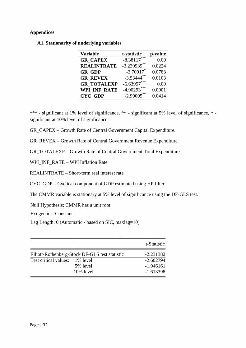
A1. Stationarity of underlying variables

Variable t-statistic p-value

GR_CAPEX -8.38117***

0.00

REALINTRATE -3.239939**

0.0224

GR_GDP -2.70917*

0.0783

GR_REVEX -3.53444**

0.0103

GR_TOTALEXP -6.63957***

0.00

WPI_INF_RATE -4.90293***

0.0001

CYC_GDP -2.99005**

0.0414

*** - significant at 1% level of significance, ** - significant at 5% level of significance, * -

significant at 10% level of significance.

GR_CAPEX – Growth Rate of Central Government Capital Expenditure.

GR_REVEX – Growth Rate of Central Government Revenue Expenditure.

GR_TOTALEXP – Growth Rate of Central Government Total Expenditure.

WPI_INF_RATE – WPI Inflation Rate

REALINTRATE – Short-term real interest rate

CYC_GDP – Cyclical component of GDP estimated using HP filter

The CMMR variable is stationary at 5% level of significance using the DF-GLS test.

Null Hypothesis: CMMR has a unit root

Exogenous: Constant

Lag Length: 0 (Automatic - based on SIC, maxlag=10)

t-Statistic

Elliott-Rothenberg-Stock DF-GLS test statistic -2.231382

Test critical values: 1% level -2.602794

5% level -1.946161

10% level -1.613398

Page | 33

A2. Hodrick-Prescott Filter

The Hodrick-Prescott (HP) filter is a technique widely used in macroeconomics to

obtain a smooth estimate of the long-term trend component of the series.7 HP filter is

a two-sided filter that estimates a smoothed series t of a time series z by minimizing

the variance of z around t, subject to a penalty that constrains the second difference of

t, i.e. the HP filter chooses t to minimize:

∑( ) ∑(( ) ( ))

is also known as the ‘penalty’ parameter, which controls the smoothness of the

series. Larger the , the smoother the series. As , t approaches a linear trend.

For annual data, and for quarterly data, .

A3. Structural VAR Analysis

Figure A1(a): IRF Capex: Including supply shocks

7Hodrick, Robert; Prescott, Edward C., "Postwar U.S. Business Cycles: An Empirical Investigation", Journal

of Money, Credit, and Banking, Vol. 29(1), pp. 1-16 (1997).

Re

sp

on

se

s o

f

Inflation

GDP Growth

Capex Growth

AS

AS

AD

AD

Capex Growth

Capex Growth

0 1 2 3 4 5 6 7 8 9-0.75

-0.50

-0.25

0.00

0.25

0.50

0.75

1.00

1.25

1.50

0 1 2 3 4 5 6 7 8 9-0.75

-0.50

-0.25

0.00

0.25

0.50

0.75

1.00

1.25

1.50

0 1 2 3 4 5 6 7 8 9-0.75

-0.50

-0.25

0.00

0.25

0.50

0.75

1.00

1.25

1.50

0 1 2 3 4 5 6 7 8 9-1.0

-0.5

0.0

0.5

1.0

1.5

0 1 2 3 4 5 6 7 8 9-1.0

-0.5

0.0

0.5

1.0

1.5

0 1 2 3 4 5 6 7 8 9-1.0

-0.5

0.0

0.5

1.0

1.5

0 1 2 3 4 5 6 7 8 9-60

-40

-20

0

20

40

60

80

0 1 2 3 4 5 6 7 8 9-60

-40

-20

0

20

40

60

80

0 1 2 3 4 5 6 7 8 9-60

-40

-20

0

20

40

60

80

Page | 34

Table A1 (a) – VDA Capex: Including supply shocks

Decomposition of Variance for Series ‘Inflation’

Step Std Error AS shocks AD shocks Capex Growth shocks

1 1.312979 95.456 2.248 2.295

2 1.6748549 96.111 1.609 2.28

3 1.8050817 96.524 1.388 2.088

4 1.8581852 96.677 1.327 1.996

5 1.8800232 96.709 1.339 1.952

6 1.8889654 96.692 1.374 1.934

7 1.8925984 96.662 1.41 1.928

8 1.8940699 96.634 1.439 1.927

9 1.8946715 96.614 1.458 1.927

10 1.8949246 96.6 1.471 1.929

Decomposition of Variance for Series ‘GDP Growth’

Step Std Error AS shocks AD shocks Capex Growth shocks

1 1.3027513 0.064 95.941 3.995

2 1.6931268 3.881 86.474 9.645

3 1.8748531 6.582 82.674 10.744

4 1.9706245 8.667 80.229 11.104

5 2.0222303 10.149 78.64 11.211

6 2.0500828 11.136 77.633 11.231

7 2.0649777 11.757 77.019 11.224

8 2.0728312 12.131 76.657 11.212

9 2.0769042 12.347 76.452 11.201

10 2.0789798 12.467 76.339 11.194

Decomposition of Variance for Series ‘Capex Growth’

Step Std Error AS shocks AD shocks Capex Growth Shocks

1 70.0588299 17.076 0 82.924

2 70.431612 17.427 0.02 82.553

3 70.4588316 17.485 0.025 82.49

4 70.4741001 17.518 0.027 82.455

5 70.4808801 17.533 0.027 82.44

6 70.4838994 17.54 0.027 82.433

7 70.4852157 17.543 0.027 82.43

8 70.4857789 17.544 0.027 82.429

9 70.4860154 17.545 0.027 82.428

10 70.486113 17.545 0.027 82.428

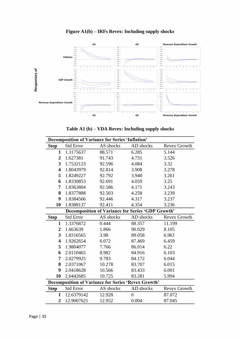
Page | 35

Figure A1(b) – IRFs Revex: Including supply shocks

Table A1 (b) – VDA Revex: Including supply shocks

Decomposition of Variance for Series ‘Inflation’

Step Std Error AS shocks AD shocks Revex Growth

1 1.3175637 88.571 6.285 5.144

2 1.627381 91.743 4.731 3.526

3 1.7532123 92.596 4.084 3.32

4 1.8043979 92.814 3.908 3.278

5 1.8249227 92.792 3.948 3.261

6 1.8330853 92.691 4.059 3.25

7 1.8363804 92.586 4.171 3.243

8 1.8377888 92.503 4.258 3.239

9 1.8384566 92.446 4.317 3.237

10 1.8388137 92.411 4.354 3.236

Decomposition of Variance for Series ‘GDP Growth’

Step Std Error AS shocks AD shocks Revex Growth

1 1.3376872 0.444 88.357 11.199

2 1.663639 1.866 90.029 8.105

3 1.8316565 3.98 89.058 6.961

4 1.9262654 6.072 87.469 6.459

5 1.9804077 7.766 86.014 6.22

6 2.0110465 8.982 84.916 6.103

7 2.0279925 9.783 84.172 6.044

8 2.0371067 10.278 83.707 6.015

9 2.0418628 10.566 83.433 6.001

10 2.0442685 10.725 83.281 5.994

Decomposition of Variance for Series ‘Revex Growth’

Step Std Error AS shocks AD shocks Revex Growth

1 12.6379142 12.928 0 87.072

2 12.9067621 12.952 0.004 87.045

Re

sp

on

se

s o

f

Inflation

GDP Growth

Revenue Expenditure Growth

AS

AS

AD

AD

Revenue Expenditure Growth

Revenue Expenditure Growth

0 1 2 3 4 5 6 7 8 9-0.75

-0.50

-0.25

0.00

0.25

0.50

0.75

1.00

1.25

1.50

0 1 2 3 4 5 6 7 8 9-0.75

-0.50

-0.25

0.00

0.25

0.50

0.75

1.00

1.25

1.50

0 1 2 3 4 5 6 7 8 9-0.75

-0.50

-0.25

0.00

0.25

0.50

0.75

1.00

1.25

1.50

0 1 2 3 4 5 6 7 8 9-0.75

-0.50

-0.25

0.00

0.25

0.50

0.75

1.00

1.25

1.50

0 1 2 3 4 5 6 7 8 9-0.75

-0.50

-0.25

0.00

0.25

0.50

0.75

1.00

1.25

1.50

0 1 2 3 4 5 6 7 8 9-0.75

-0.50

-0.25

0.00

0.25

0.50

0.75

1.00

1.25

1.50

0 1 2 3 4 5 6 7 8 9-7.5

-5.0

-2.5

0.0

2.5

5.0

7.5

10.0

12.5

15.0

0 1 2 3 4 5 6 7 8 9-7.5

-5.0

-2.5

0.0

2.5

5.0

7.5

10.0

12.5

15.0

0 1 2 3 4 5 6 7 8 9-7.5

-5.0

-2.5

0.0

2.5

5.0

7.5

10.0

12.5

15.0

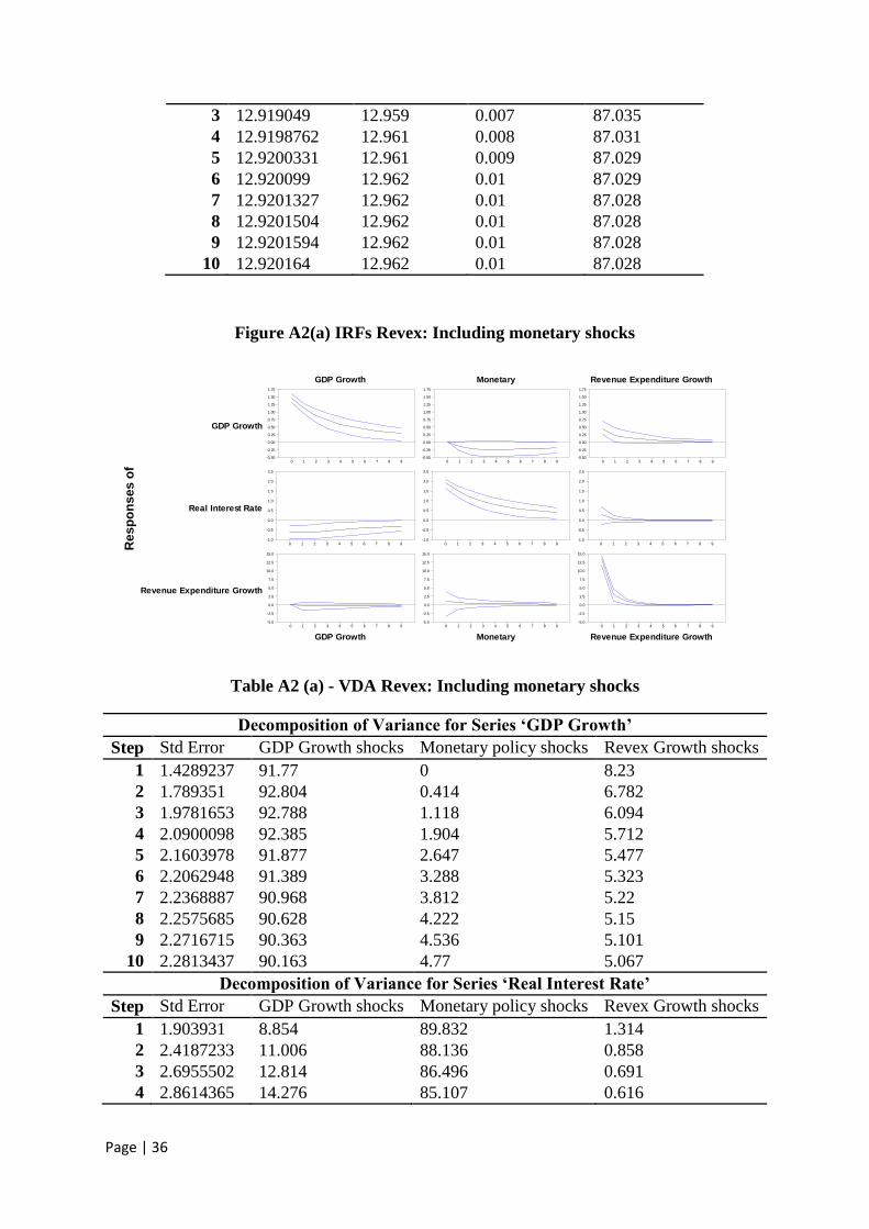
Page | 36

3 12.919049 12.959 0.007 87.035

4 12.9198762 12.961 0.008 87.031

5 12.9200331 12.961 0.009 87.029

6 12.920099 12.962 0.01 87.029

7 12.9201327 12.962 0.01 87.028

8 12.9201504 12.962 0.01 87.028

9 12.9201594 12.962 0.01 87.028

10 12.920164 12.962 0.01 87.028

Figure A2(a) IRFs Revex: Including monetary shocks

Table A2 (a) - VDA Revex: Including monetary shocks

Decomposition of Variance for Series ‘GDP Growth’

Step Std Error GDP Growth shocks Monetary policy shocks Revex Growth shocks

1 1.4289237 91.77 0 8.23

2 1.789351 92.804 0.414 6.782

3 1.9781653 92.788 1.118 6.094

4 2.0900098 92.385 1.904 5.712

5 2.1603978 91.877 2.647 5.477

6 2.2062948 91.389 3.288 5.323

7 2.2368887 90.968 3.812 5.22

8 2.2575685 90.628 4.222 5.15

9 2.2716715 90.363 4.536 5.101

10 2.2813437 90.163 4.77 5.067

Decomposition of Variance for Series ‘Real Interest Rate’

Step Std Error GDP Growth shocks Monetary policy shocks Revex Growth shocks

1 1.903931 8.854 89.832 1.314

2 2.4187233 11.006 88.136 0.858

3 2.6955502 12.814 86.496 0.691

4 2.8614365 14.276 85.107 0.616

Re

sp

on

se

s o

f

GDP Growth

Real Interest Rate

Revenue Expenditure Growth

GDP Growth

GDP Growth

Monetary

Monetary

Revenue Expenditure Growth

Revenue Expenditure Growth

0 1 2 3 4 5 6 7 8 9-0.50

-0.25

0.00

0.25

0.50

0.75

1.00

1.25

1.50

1.75

0 1 2 3 4 5 6 7 8 9-0.50

-0.25

0.00

0.25

0.50

0.75

1.00

1.25

1.50

1.75

0 1 2 3 4 5 6 7 8 9-0.50

-0.25

0.00

0.25

0.50

0.75

1.00

1.25

1.50

1.75

0 1 2 3 4 5 6 7 8 9-1.0

-0.5

0.0

0.5

1.0

1.5

2.0

2.5

0 1 2 3 4 5 6 7 8 9-1.0

-0.5

0.0

0.5

1.0

1.5

2.0

2.5

0 1 2 3 4 5 6 7 8 9-1.0

-0.5

0.0

0.5

1.0

1.5

2.0

2.5

0 1 2 3 4 5 6 7 8 9-5.0

-2.5

0.0

2.5

5.0

7.5

10.0

12.5

15.0

0 1 2 3 4 5 6 7 8 9-5.0

-2.5

0.0

2.5

5.0

7.5

10.0

12.5

15.0

0 1 2 3 4 5 6 7 8 9-5.0

-2.5

0.0

2.5

5.0

7.5

10.0

12.5

15.0

Page | 37

5 2.9662197 15.424 83.996 0.58

6 3.0344843 16.303 83.135 0.562

7 3.0798349 16.963 82.485 0.553

8 3.1103507 17.451 82.001 0.548

9 3.1310605 17.808 81.647 0.546

10 3.1451969 18.066 81.39 0.544

Decomposition of Variance for Series ‘Revenue Expenditure Growth’

Step Std Error GDP Growth shocks Monetary policy shocks Revex Growth shocks

1 12.7241453 0 0.03 99.97

2 13.025273 0.065 0.16 99.776

3 13.0498405 0.139 0.273 99.588

4 13.059365 0.199 0.353 99.449

5 13.0657556 0.243 0.406 99.351

6 13.0701766 0.275 0.441 99.284

7 13.0732274 0.297 0.465 99.238

8 13.0753314 0.313 0.48 99.206

9 13.076783 0.324 0.491 99.184

10 13.0777852 0.332 0.498 99.169

Figure A2 (b) - IRFs Capex: Including monetary shocks

Table A2(b)- VDA Capex: Including monetary shocks

Decomposition of Variance for Series ‘GDP Growth’

Step Std Error GDP Growth Monetary policy shocks Capex Growth shocks

1 1.3713185 96.729 0 3.271

2 1.7973393 86.589 0.506 12.904

3 1.9994638 83.693 1.143 15.164

4 2.1131943 81.951 1.789 16.26

Re

sp

on

se

s o

f

GDP Growth

Real Interest Rate

Capex Growth

GDP Growth

GDP Growth

Monetary

Monetary

Capex Growth

Capex Growth

0 1 2 3 4 5 6 7 8 9-0.50

-0.25

0.00

0.25

0.50

0.75

1.00

1.25

1.50

1.75

0 1 2 3 4 5 6 7 8 9-0.50

-0.25

0.00

0.25

0.50

0.75

1.00

1.25

1.50

1.75

0 1 2 3 4 5 6 7 8 9-0.50

-0.25

0.00

0.25

0.50

0.75

1.00

1.25

1.50

1.75

0 1 2 3 4 5 6 7 8 9-1.0

-0.5

0.0

0.5

1.0

1.5

2.0

2.5

0 1 2 3 4 5 6 7 8 9-1.0

-0.5

0.0

0.5

1.0

1.5

2.0

2.5

0 1 2 3 4 5 6 7 8 9-1.0

-0.5

0.0

0.5

1.0

1.5

2.0

2.5

0 1 2 3 4 5 6 7 8 9-20

0

20

40

60

80

100

0 1 2 3 4 5 6 7 8 9-20

0

20

40

60

80

100

0 1 2 3 4 5 6 7 8 9-20

0

20

40

60

80

100

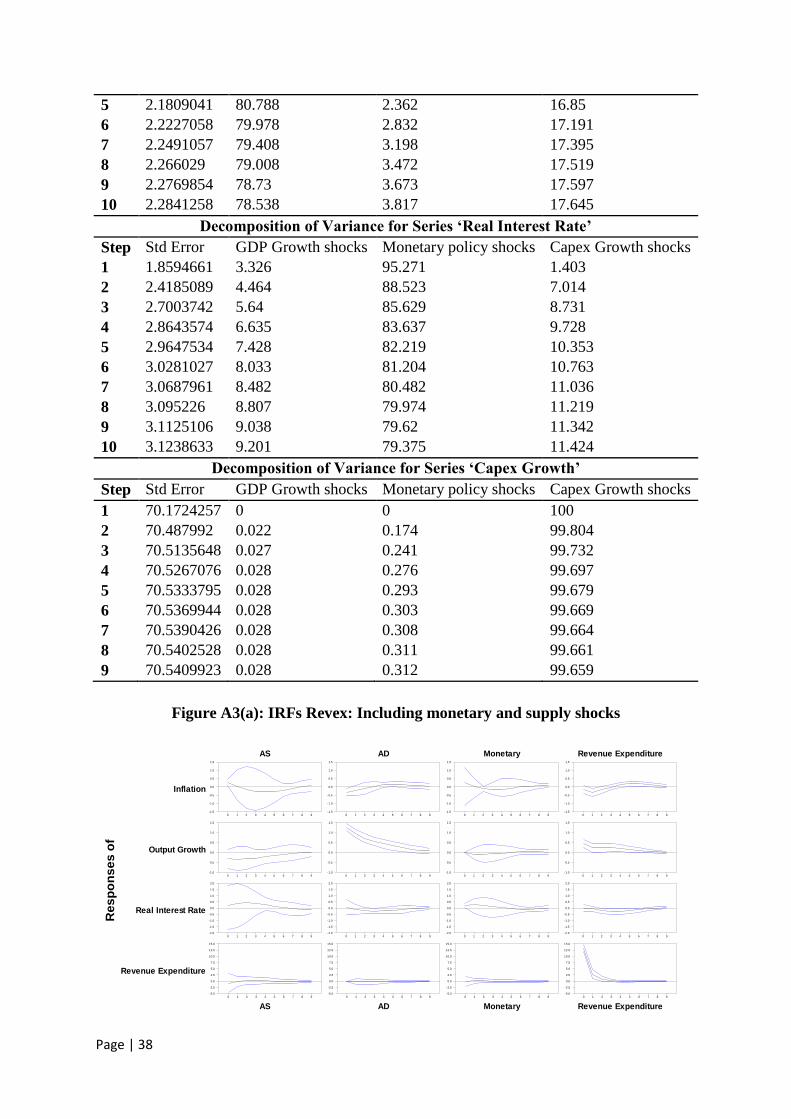
Page | 38

5 2.1809041 80.788 2.362 16.85

6 2.2227058 79.978 2.832 17.191

7 2.2491057 79.408 3.198 17.395

8 2.266029 79.008 3.472 17.519

9 2.2769854 78.73 3.673 17.597

10 2.2841258 78.538 3.817 17.645

Decomposition of Variance for Series ‘Real Interest Rate’

Step Std Error GDP Growth shocks Monetary policy shocks Capex Growth shocks

1 1.8594661 3.326 95.271 1.403

2 2.4185089 4.464 88.523 7.014

3 2.7003742 5.64 85.629 8.731

4 2.8643574 6.635 83.637 9.728

5 2.9647534 7.428 82.219 10.353

6 3.0281027 8.033 81.204 10.763

7 3.0687961 8.482 80.482 11.036

8 3.095226 8.807 79.974 11.219

9 3.1125106 9.038 79.62 11.342

10 3.1238633 9.201 79.375 11.424

Decomposition of Variance for Series ‘Capex Growth’

Step Std Error GDP Growth shocks Monetary policy shocks Capex Growth shocks

1 70.1724257 0 0 100

2 70.487992 0.022 0.174 99.804

3 70.5135648 0.027 0.241 99.732

4 70.5267076 0.028 0.276 99.697

5 70.5333795 0.028 0.293 99.679

6 70.5369944 0.028 0.303 99.669

7 70.5390426 0.028 0.308 99.664

8 70.5402528 0.028 0.311 99.661

9 70.5409923 0.028 0.312 99.659

Figure A3(a): IRFs Revex: Including monetary and supply shocks

Re

sp

on

se

s o

f

Inflation

Output Growth

Real Interest Rate

Revenue Expenditure

AS

AS

AD

AD

Monetary

Monetary

Revenue Expenditure

Revenue Expenditure

0 1 2 3 4 5 6 7 8 9-1.5

-1.0

-0.5

0.0

0.5

1.0

1.5

0 1 2 3 4 5 6 7 8 9-1.5

-1.0

-0.5

0.0

0.5

1.0

1.5

0 1 2 3 4 5 6 7 8 9-1.5

-1.0

-0.5

0.0

0.5

1.0

1.5

0 1 2 3 4 5 6 7 8 9-1.5

-1.0

-0.5

0.0

0.5

1.0

1.5

0 1 2 3 4 5 6 7 8 9-1.0

-0.5

0.0

0.5

1.0

1.5

0 1 2 3 4 5 6 7 8 9-1.0

-0.5

0.0

0.5

1.0

1.5

0 1 2 3 4 5 6 7 8 9-1.0

-0.5

0.0

0.5

1.0

1.5

0 1 2 3 4 5 6 7 8 9-1.0

-0.5

0.0

0.5

1.0

1.5

0 1 2 3 4 5 6 7 8 9-2.0

-1.5

-1.0

-0.5

0.0

0.5

1.0

1.5

2.0

0 1 2 3 4 5 6 7 8 9-2.0

-1.5

-1.0

-0.5

0.0

0.5

1.0

1.5

2.0

0 1 2 3 4 5 6 7 8 9-2.0

-1.5

-1.0

-0.5

0.0

0.5

1.0

1.5

2.0

0 1 2 3 4 5 6 7 8 9-2.0

-1.5

-1.0

-0.5

0.0

0.5

1.0

1.5

2.0

0 1 2 3 4 5 6 7 8 9-5.0

-2.5

0.0

2.5

5.0

7.5

10.0

12.5

15.0

0 1 2 3 4 5 6 7 8 9-5.0

-2.5

0.0

2.5

5.0

7.5

10.0

12.5

15.0

0 1 2 3 4 5 6 7 8 9-5.0

-2.5

0.0

2.5

5.0

7.5

10.0

12.5

15.0

0 1 2 3 4 5 6 7 8 9-5.0

-2.5

0.0

2.5

5.0

7.5

10.0

12.5

15.0

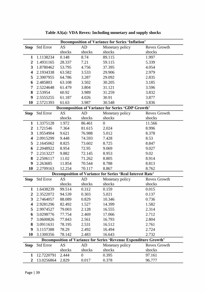
Page | 39

Table A3(a): VDA Revex: Including monetary and supply shocks

Decomposition of Variance for Series ‘Inflation’

Step Std Error AS

shocks

AD

shocks

Monetary policy

shocks

Revex Growth

shocks

1 1.1138234 0.148 8.74 89.115 1.997

2 1.4931165 28.337 7.21 59.115 5.339

3 1.8780462 53.795 4.756 37.395 4.054

4 2.1934338 63.582 3.533 29.906 2.979

5 2.3907955 64.786 3.287 29.092 2.835

6 2.485803 63.108 3.502 30.205 3.185

7 2.5224648 61.479 3.804 31.121 3.596

8 2.53954 60.92 3.989 31.259 3.832

9 2.5555255 61.187 4.026 30.91 3.877

10 2.5721393 61.63 3.987 30.548 3.836

Decomposition of Variance for Series ‘GDP Growth’

Step Std Error AS

shocks

AD

shocks

Monetary policy

shocks

Revex Growth

shocks

1 1.3375128 1.972 86.461 0 11.566

2 1.721546 7.364 81.615 2.024 8.996

3 1.9554904 9.621 76.988 5.012 8.378

4 2.0915299 9.448 74.593 7.428 8.53

5 2.1645062 8.825 73.602 8.725 8.847

6 2.2048922 8.954 72.95 9.069 9.027

7 2.2313227 9.882 72.145 8.953 9.02

8 2.2506117 11.02 71.262 8.805 8.914

9 2.263685 11.854 70.544 8.788 8.813

10 2.2709163 12.254 70.117 8.867 8.762

Decomposition of Variance for Series ‘Real Interest Rate’

Step Std Error AS

shocks

AD

shocks

Monetary policy

shocks

Revex Growth

shocks

1 1.6438239 99.514 0.312 0.159 0.015

2 2.3522072 94.539 0.303 5.021 0.137

3 2.7464057 88.089 0.829 10.346 0.736

4 2.9281296 82.492 1.527 14.399 1.582

5 2.9974527 79.003 2.128 16.555 2.314

6 3.0298776 77.754 2.469 17.066 2.712

7 3.0600826 77.843 2.561 16.793 2.804

8 3.0911631 78.195 2.531 16.512 2.761

9 3.1157388 78.29 2.492 16.494 2.724

10 3.1300356 78.142 2.483 16.643 2.732

Decomposition of Variance for Series ‘Revenue Expenditure Growth’

Step Std Error AS

shocks

AD

shocks

Monetary policy

shocks

Revex Growth

shocks

1 12.7220791 2.444 0 0.395 97.161

2 13.0256864 2.829 0.017 0.378 96.777

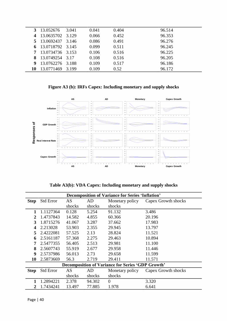
Page | 40

3 13.052676 3.041 0.041 0.404 96.514

4 13.0635702 3.129 0.066 0.452 96.353

5 13.0692437 3.146 0.086 0.491 96.276

6 13.0718792 3.145 0.099 0.511 96.245

7 13.0734736 3.153 0.106 0.516 96.225

8 13.0749254 3.17 0.108 0.516 96.205

9 13.0762276 3.188 0.109 0.517 96.186

10 13.0771469 3.199 0.109 0.52 96.172

Figure A3 (b): IRFs Capex: Including monetary and supply shocks

Table A3(b): VDA Capex: Including monetary and supply shocks

Decomposition of Variance for Series ‘Inflation’

Step Std Error AS

shocks

AD

shocks

Monetary policy

shocks

Capex Growth shocks

1 1.1127364 0.128 5.254 91.132 3.486

2 1.4737843 14.582 4.855 60.366 20.196

3 1.8715276 41.067 3.287 37.662 17.983

4 2.213028 53.903 2.355 29.945 13.797

5 2.4222081 57.525 2.13 28.824 11.521

6 2.5161187 57.368 2.275 29.463 10.894

7 2.5477355 56.405 2.513 29.981 11.100

8 2.5607743 55.919 2.677 29.958 11.446

9 2.5737986 56.013 2.73 29.658 11.599

10 2.5873669 56.3 2.719 29.411 11.571

Decomposition of Variance for Series ‘GDP Growth’

Step Std Error AS

shocks

AD

shocks

Monetary policy

shocks

Capex Growth shocks

1 1.2894221 2.378 94.302 0 3.320

2 1.7434241 13.497 77.885 1.978 6.641

Re

sp

on

se

s o

f

Inflation

GDP Growth

Real Interest Rate

Capex Growth

AS

AS

AD

AD

Monetary

Monetary

Capex Growth

Capex Growth

0 1 2 3 4 5 6 7 8 9-1.5

-1.0

-0.5

0.0

0.5

1.0

1.5

0 1 2 3 4 5 6 7 8 9-1.5

-1.0

-0.5

0.0

0.5

1.0

1.5

0 1 2 3 4 5 6 7 8 9-1.5

-1.0

-0.5

0.0

0.5

1.0

1.5

0 1 2 3 4 5 6 7 8 9-1.5

-1.0

-0.5

0.0

0.5

1.0

1.5

0 1 2 3 4 5 6 7 8 9-1.5

-1.0

-0.5

0.0

0.5

1.0

1.5

0 1 2 3 4 5 6 7 8 9-1.5

-1.0

-0.5

0.0

0.5

1.0

1.5

0 1 2 3 4 5 6 7 8 9-1.5

-1.0

-0.5

0.0

0.5

1.0

1.5

0 1 2 3 4 5 6 7 8 9-1.5

-1.0

-0.5

0.0

0.5

1.0

1.5

0 1 2 3 4 5 6 7 8 9-2.0

-1.5

-1.0

-0.5

0.0

0.5

1.0

1.5

2.0

0 1 2 3 4 5 6 7 8 9-2.0

-1.5

-1.0

-0.5

0.0

0.5

1.0

1.5

2.0

0 1 2 3 4 5 6 7 8 9-2.0

-1.5

-1.0

-0.5

0.0

0.5

1.0

1.5

2.0

0 1 2 3 4 5 6 7 8 9-2.0

-1.5

-1.0

-0.5

0.0

0.5

1.0

1.5

2.0

0 1 2 3 4 5 6 7 8 9-60

-40

-20

0

20

40

60

80

0 1 2 3 4 5 6 7 8 9-60

-40

-20

0

20

40

60

80

0 1 2 3 4 5 6 7 8 9-60

-40

-20

0

20

40

60

80

0 1 2 3 4 5 6 7 8 9-60

-40

-20

0

20

40

60

80

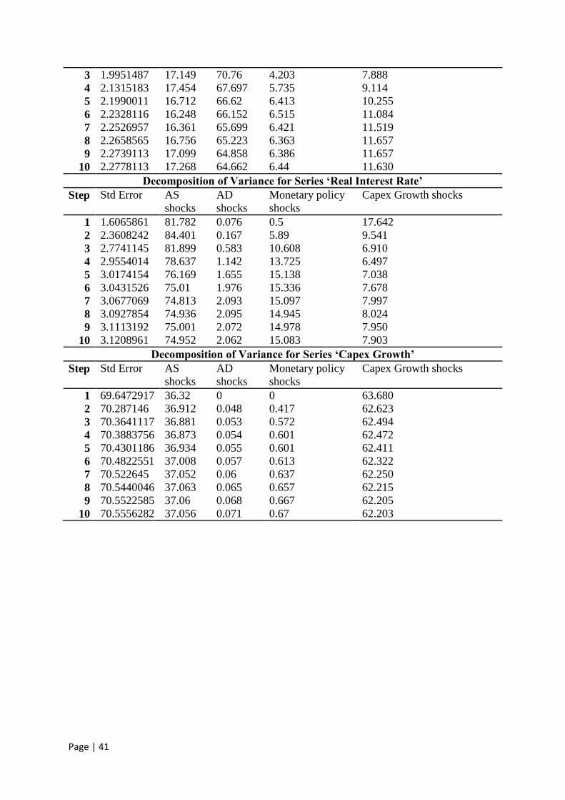
Page | 41

3 1.9951487 17.149 70.76 4.203 7.888

4 2.1315183 17.454 67.697 5.735 9.114

5 2.1990011 16.712 66.62 6.413 10.255

6 2.2328116 16.248 66.152 6.515 11.084

7 2.2526957 16.361 65.699 6.421 11.519

8 2.2658565 16.756 65.223 6.363 11.657

9 2.2739113 17.099 64.858 6.386 11.657

10 2.2778113 17.268 64.662 6.44 11.630

Decomposition of Variance for Series ‘Real Interest Rate’

Step Std Error AS

shocks

AD

shocks

Monetary policy

shocks

Capex Growth shocks

1 1.6065861 81.782 0.076 0.5 17.642

2 2.3608242 84.401 0.167 5.89 9.541

3 2.7741145 81.899 0.583 10.608 6.910

4 2.9554014 78.637 1.142 13.725 6.497

5 3.0174154 76.169 1.655 15.138 7.038

6 3.0431526 75.01 1.976 15.336 7.678

7 3.0677069 74.813 2.093 15.097 7.997

8 3.0927854 74.936 2.095 14.945 8.024

9 3.1113192 75.001 2.072 14.978 7.950

10 3.1208961 74.952 2.062 15.083 7.903

Decomposition of Variance for Series ‘Capex Growth’

Step Std Error AS

shocks

AD

shocks

Monetary policy

shocks

Capex Growth shocks

1 69.6472917 36.32 0 0 63.680

2 70.287146 36.912 0.048 0.417 62.623

3 70.3641117 36.881 0.053 0.572 62.494

4 70.3883756 36.873 0.054 0.601 62.472

5 70.4301186 36.934 0.055 0.601 62.411

6 70.4822551 37.008 0.057 0.613 62.322

7 70.522645 37.052 0.06 0.637 62.250

8 70.5440046 37.063 0.065 0.657 62.215

9 70.5522585 37.06 0.068 0.667 62.205

10 70.5556282 37.056 0.071 0.67 62.203