www.ssoar.info
Computing weights for the German LongitudinalElection Study (GLES) 2009-2013Gummer, Tobias; Blumenberg, Manuela S.; Vilgis, Constanze
Veröffentlichungsversion / Published VersionArbeitspapier / working paper
Zur Verfügung gestellt in Kooperation mit / provided in cooperation with:GESIS - Leibniz-Institut für Sozialwissenschaften
Empfohlene Zitierung / Suggested Citation:Gummer, Tobias ; Blumenberg, Manuela S. ; Vilgis, Constanze ; GESIS - Leibniz-Institut für Sozialwissenschaften(Ed.): Computing weights for the German Longitudinal Election Study (GLES) 2009-2013. Köln, 2017 (GESIS Papers2017/07). URN: http://nbn-resolving.de/urn:nbn:de:0168-ssoar-50704-4
Nutzungsbedingungen:Dieser Text wird unter einer CC BY-NC Lizenz (Namensnennung-Nicht-kommerziell) zur Verfügung gestellt. Nähere Auskünfte zuden CC-Lizenzen finden Sie hier:https://creativecommons.org/licenses/by-nc/4.0/deed.de
Terms of use:This document is made available under a CC BY-NC Licence(Attribution-NonCommercial). For more Information see:https://creativecommons.org/licenses/by-nc/4.0/

Computing weights for the German Longitudinal Election Study (GLES) 2009-2013
2017|07
Tobias Gummer, Manuela S. Blumenberg &
Constanze Vilgis
GESIS Papers

Computing weights for the German Longitudinal Election Study (GLES) 2009-2013
GESIS-Papers 2017|07
Tobias Gummer, Manuela S. Blumenberg & Constanze Vilgis
GESIS – Leibniz-Institut für Sozialwissenschaften 2017

GESIS-Papers
GESIS – Leibniz-Institut für Sozialwissenschaften
Dauerbeobachtung der Gesellschaft
GESIS-Projektleitung German Longitudinal Election Study
Postfach 12 21 55
68072 Mannheim
Telefon: (0621) 1246 - 502
Telefax: (0221) 1246 - 530
E-Mail: [email protected]
ISSN: 2364-3773 (Print)
ISSN: 2364-3781 (Online)
Herausgeber,
Druck und Vertrieb: GESIS – Leibniz-Institut für Sozialwissenschaften
Unter Sachsenhausen 6-8, 50667 Köln

Contents
1 Introduction ....................................................................................................................................................... 5
2 Design weights ................................................................................................................................................... 7
3 Adjustment weights .......................................................................................................................................... 9
3.1 Iterative proportional fitting............................................................................................................... 9
3.2 Operationalization..............................................................................................................................10
4 Panel weights ...................................................................................................................................................14
4.1 Propensity score weighting ...............................................................................................................14
4.2 Predictors of response propensities .................................................................................................15
4.3 Propensity models ..............................................................................................................................16
5 Remarks on the use of weighting..................................................................................................................23
References ..............................................................................................................................................................25
Data sets .................................................................................................................................................................28
Appendix .................................................................................................................................................................30


Computing weights for the German Longitudinal Election Study (GLES) 2009-2013 5
1 Introduction1,2
The German Longitudinal Election Study (GLES) is a research project funded by the DFG that began with the German federal election in 2009. Up until now, it is the biggest German national election study and aims to observe and analyze the German electorate at three consecutive federal elections, starting with the election in 2009. It is envisaged that the research project will continue after 2017 as an institutionalized German election study.
In 2009, the study was launched by Prof. Dr. Hans Rattinger (University of Mannheim), Prof. Dr. Sigrid Roßteutscher (University of Frankfurt), Prof. Dr. Rüdiger Schmitt-Beck (University of Mannheim), and Prof. Dr. Bernhard Weßels (Social Science Research Center, Berlin). At present, the study is managed by Prof. Dr. Sigrid Roßteutscher, Prof. Dr. Rüdiger Schmitt-Beck, Prof. Dr. Harald Schoen (Mannheim Cen-tre for European Social Research), Prof. Dr. Bernhard Weßels (Social Science Research Center, Berlin), and Prof. Dr. Christof Wolf (GESIS). The principal investigators are conducting the study in close coop-eration with the German Society for Electoral Studies (DGfW) and the GESIS – Leibniz Institute for the Social Sciences.
In order to observe short-term as well as long-term dynamics within the electorate, a complex project design was developed for the GLES (see Figure 1). This resulted in a mix of different research methods (surveys, content analysis, experiments). These methods partly link quantitative and qualitative ele-ments. Furthermore, different types of survey design (cross-sections, rolling cross-sections, and panels), as well as interview techniques (CATI, CAPI, PAPI, web), are applied to collect data at an individual level.
Figure 1: Overview of the GLES design, 2009 and 2013
1 The present report is strongly based on the following previously published reports: “Gewichtung in der German
Longitudinal Election Study 2009” (Blumenberg & Gummer, 2013) and “Gewichtung in der German Longitudinal election Study 2013” (Blumenberg & Gummer, 2016).
2 We would like to thank Patrik Haffner for his valuable assistance when preparing this report.
6 GESIS Papers 2017|07
During data preparation, GLES data is enriched with additional information, such as weighting factors. This technical report provides a general discussion of the computation of weights that was done in the context of the 2009 and 2013 data collection efforts. Further information about the weights can be found in the study descriptions of the respective GLES data sets.
The basic idea of providing users with pre-calculated weights was to ensure homogeneity between the different parts of the GLES, while considering the specific context of the different components. For instance, one issue is that it might not be possible to calculate similar weights for studies with differ-ent survey modes. This can severely hinder comparison between these two studies, as applying differ-ent weights might introduce additional differences between the studies. In the GLES, efforts were taken to use a consistent approach when computing weights for different components. These efforts aim at easing inter-component comparisons by reducing the influence that the use of weights (pre-sumably) has on discrepancies between these components. Furthermore, the calculation of similar weights makes GLES data more readily assessable. In other words, users are required to make less effort to understand how weights were computed for several components of the GLES, as similar methods were applied throughout.
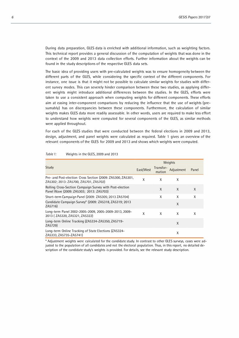
For each of the GLES studies that were conducted between the federal elections in 2009 and 2013, design, adjustment, and panel weights were calculated as required. Table 1 gives an overview of the relevant components of the GLES for 2009 and 2013 and shows which weights were computed.
Table 1: Weights in the GLES, 2009 and 2013
Study Weights
East/West Transfor-mation Adjustment Panel
Pre- and Post-election Cross Section (2009: ZA5300, ZA5301, ZA5302; 2013: ZA5700, ZA5701, ZA5702) X X X
Rolling Cross-Section Campaign Survey with Post-election Panel Wave (2009: ZA5303; 2013: ZA5703) X X X
Short-term Campaign Panel (2009: ZA5305; 2013 ZA5704) X X X Candidate Campaign Survey* (2009: ZA5318, ZA5319; 2013 ZA5716) X
Long-term Panel 2002-2005-2009, 2005-2009-2013, 2009-2013 ( ZA5320, ZA5321, ZA5322) X X X X
Long-term Online Tracking (ZA5334-ZA5350, ZA5719-ZA5729) X
Long-term Online Tracking of State Elections (ZA5324-ZA5333, ZA5735-ZA5741) X
* Adjustment weights were calculated for the candidate study. In contrast to other GLES surveys, cases were ad-justed to the population of all candidates and not the electoral population. Thus, in this report, no detailed de-scription of the candidate study’s weights is provided. For details, see the relevant study description.
Computing weights for the German Longitudinal Election Study (GLES) 2009-2013 7
2 Design weights
Design weights can tackle biases introduced by the survey design. Within the GLES, design weights are calculated in order to correct selective overrepresentation of eastern German respondents. Other design weights, like a transformation weight, can be used to transform a household sample into a person sam-ple (Schumann, 2012, p. 101f). For some parts of the GLES study, both weights (i.e., east/west and transformation) were calculated.
For both federal elections in 2009 and 2013, the east/west weight was calculated for the pre- and post-election cross-section surveys, as well as for the first wave in the long-term panel survey. In these studies, an oversampling of the population in the new federal states (including Berlin) was implemented to allow for analyses of subgroups in eastern Germany. The east/west weight can help to account for the disproportionality of the sample and permit generalized estimates for the whole of Germany.
In order to calculate the east/west weight, cell weighting was used to adjust the survey data to distribu-tions taken from the German Micro Census of 2009 (for the election in 2009) and the Micro Census of 2012 (for the election in 2013). Only people aged 16 years or older (respectively 18 years of age) that held German citizenship and resided in private households at the location of the principal domicile were considered.3
The east/west weight 𝑤𝑒𝑒 was calculated as the ratio between the relative frequencies of the respond-ents in either one of the regions in the survey (ℎ�𝑒/𝑒 ) and the respective true relative frequencies (ℎ𝑒/𝑒).
𝑤𝑒𝑒 =
⎩⎪⎨
⎪⎧ℎ𝑒ℎ�𝑒
𝑖𝑖 𝑒𝑒𝑒𝑒 = 1
ℎ𝑒ℎ�𝑒
𝑖𝑖 𝑒𝑒𝑒𝑒 = 0
Accordingly, respondents in eastern Germany (including Berlin) received a weighting factor below one, while respondents in the old federal states received a factor slightly above 1.
Several components of the GLES are not only based on person samples but on household samples. In face-to-face and telephone samples, individuals in households of different sizes do not have the same probability for participating in the survey. The larger the household, the smaller the probability is for an individual to be selected for the survey. This issue concerns the cross-sections and rolling cross-section surveys. Hence, transformation weights are provided for these surveys. Transformation weights provide a tool to correct for different selection probabilities within households. The weights are based on a reduced household size. That is, only people belonging to the target population are considered. For instance, if a household consists of four people older than 16 years of age, each person in this household has a 25% chance of being selected. However, if a household is comprised of two individu-als older than 16 years of age, each has a 50% probability of being selected.
The calculation of the transformation weights is straightforward – respondents receive a factor corre-sponding to their inverted selection probability. For the cross-section surveys, the reduced household size was used to calculate the probabilities, while the number of telephone connections was used in
3 In every component of the GLES, except the rolling cross section and the long-term-panel from 2005-2009-
2013, people over 18 years of age or older who hold German citizenship were defined as the target population. In the cross sections, as well as the long-term panel from 2002-2005-2009, the minimum age was 16.

8 GESIS Papers 2017|07
the case of the telephone surveys. Finally, the weights were standardized to a mean of 1 in order to keep the sample size the same. 4
4 The use of transformation weights is controversially discussed in the social sciences. Some argue that transfor-
mation weights are necessary, due to the sampling procedure. Others claim that biases which are corrected by transformation weights are counteract another bias, which is generated by the fact that smaller households are more difficult to reach than larger ones (Arzheimer, 2009, p. 363; Hartmann & Schimpl-Neimanns, 1992; Terwey, Bens, Baumann, & Baltzer, 2007).

Computing weights for the German Longitudinal Election Study (GLES) 2009-2013 9
3 Adjustment weights
Weights can be used to adjust the distributions of a survey’s sample to the distributions in the target population. If the true distribution of the target population is known, adjustment weights may be used to calibrate the survey’s distribution. Nonresponse is one possible reason why the distributions of indi-viduals’ characteristics in a sample may significantly differ from distributions among the population (Gabler, 2004, p. 128). The intention of using these weights is to allow one to draw conclusions related to the target population, even if the sample is subject to some degree of selectivity (Faas & Schoen, 2009, p. 146).
It is important to note that, for the GLES, external references had to be used to refer to the target population’s “true” distributions. The calculation of weights for the GLES had two requirements: First, the distribution of variables that were selected for adjustment had to be available in some sort of reference study. The Micro Census of 2009 (German federal election in 2009) and the Micro Census of 2012 (German federal election in 2013) were used as reference studies, since these were considered to represent the target population most closely. Parts of the GLES were conducted web-based and, hence, the (N)Onliner Atlas for 2012 and 2014 respectively were used as reference studies for the online pop-ulation of Germany. Second, as argued above, the GLES aimed to provide similar weighting factors for different components to allow for comparisons between the different data sets. Hence, variables that were available in most of the GLES data sets were selected for computing adjustment variables.
3.1 Iterative proportional fitting
There are different procedures for computing adjustment weights. In the GLES, cell and IPF weighting (iterative proportional fitting) were used. In cell weighting, a weighting factor to adjust a sample’s distribution to the population’s distribution (i.e., the reference study) is calculated by dividing the “true” by the “actual” relative frequencies. Note that a distribution may be the distribution of a single variable or the multivariate distribution of several variables. This demands that the “true” distribution of all adjusted variables and characteristics is known. Accordingly, two problems may arise (Gabler, 2004, p. 128ff):
(i) If not only one but multiple variables are adjusted for, it is frequently the case that distribu-tions can only be known for the individual variables but not the multivariate (crossed) distribu-tions. In this case, cell weighting is not possible.
(ii) Even if the multivariate distribution with respect to all adjustment variables is known, problems may arise because of empty or sparse cells. In this case, again, simple cell weighting is not pos-sible.
When creating the east/west design weight, a cell-weighting approach was used. Assuming that a sec-ond variable is selected to create an adjustment weight for, say, the region of residence (east/west) and gender, the multivariate distribution would presumably pose no problems, as only four cells are present (east/west × female/male). If multiple additional variables are considered (e.g., age or education), the number of cells will markedly increase. As a consequence, empty or sparse cells will occur more fre-quently. One possible solution would be to group cells together to reduce the overall number of cells. However, this would result in a loss of precision and information.
IPF offers an alternative method to cell weighting for calculating adjustment weights. In this iterative adjustment procedure, based on the work of Deming and Stephan (1940), the actual distribution of the sample gets adjusted in iterative steps to the target (“true”) distribution. That is, weights are com-

10 GESIS Papers 2017|07
puted for one of the adjustment variables and are then modified to adjust for the next variable as well. In other words, the calculated weighting factor after an iteration step is the initial value for the adjustment of the next variable. The adjustment procedure is completed when the target distribution equals the actual weighted distribution. Since it may not be possible or mandatory to achieve perfect equivalence, a termination criterion can be defined. Two possible solutions define percentage differ-ences between the adjusted and target distributions or the number of iteration. A detailed discussion of the method is given by Deming und Stephan (1940, p. 428ff).
The adjustment weights of the GLES are based on five variables that have a multivariate (crossed) dis-tribution with a total of 144 cells. Accordingly, cell weighting was not feasible due to the huge num-ber of cells. Thus, in the GLES the IPF weighting was used to calculate the adjustment weights.
The weights were calculated in Stata with the user-written ipfweight command (Bergmann, 2011). In general, the algorithm mostly converges after 5 to 10 iterations. The failure to achieve convergence or a large number of iterations may point to the presence of many empty cells and/or a highly skewed sam-ple.
3.2 Operationalization
The aim of appending GLES data sets with weighting factors is to provide users with a tool to achieve equivalent distributions with respect to the target population. On the one hand, applying weights also increases variation. On the other hand, the selection of variables determines whether a bias might be reduced. A variable’s bias is only reduced if, first, the variable is indeed correlated with the adjustment variables and if, second, these adjustment variables are correlated with the source of the bias (e.g., a nonresponse process). If there is no relationship between biased variables and adjustment variables, applying weights may only conceal the problem, while not providing any substantial effect (Gabler, 2004, p. 141).
The GLES faced the challenge to calculate adjustment weights with the same procedure for different components. Therefore, the variables used for adjustment had to be available for every data set with comparable scales. Since sociodemographic variables were used for adjustment weighting (as the dis-tributions in the target population were known), this was considered a minor issue. Yet, the best way to handle missing values remained a pressing consideration in this process. One possible solution would have been to exclude cases with missing values (i.e., listwise deletion). However, this would have resulted in a subset of cases without weights and thus a reduction of the effective sample size when using weights. A different solution was the use of complex imputation procedures. Since there were only very few cases with missing values (constantly below 2%), a simple assignment of the missing values was preferred. For these cases, the modal category was assigned when calculating the weights (single imputation). As a consequence, missing values were, depending on the component, assigned to different categories (i.e., the modal categories of a variable differ between studies). However, the pro-cedure for assigning and selecting the category was always the same. For instance, take the respond-ents’ education: whereas the modal category of education in pre- and post-election cross sections was “low” education, in the RCS, the modal category was “high” education.
To ensure perfect comparability, each adjustment variable would need to be collected with identical question wording, scales, and questionnaire design. Due to the specific focus of each component and differences in survey design (e.g., mode), this was not always the case in the GLES. However, differ-ences largely remained minor as the GLES features a set of shared key questions.
Note that the adjustment weights were not calculated for specific research questions but to balance distributions of the survey data according to the target population. Furthermore, it is important to

Computing weights for the German Longitudinal Election Study (GLES) 2009-2013 11
acknowledge that only sociodemographic variables for which a reference distribution was available could be considered for calculating the weights.
Accordingly, two main rationales guided the selection of adjustment variables. First, there had to be an (assumed) relationship between the variables and the general topics of the GLES. Second, the variables had to be available in the Micro Censuses of 2009 and 2012. In the end, five adjustment variables were selected, all of which were sociodemographic variables.
Gender
Substantive variables are often analyzed for, and these analyses often highlight, differences between men and women. For example, it has been shown that women report lower levels of political interest in comparison to men and that they additionally report less involvement in traditional structures of politics (Keil & Holtz-Bacha, 2008, p. 242). Furthermore, differences can be found when looking at voting behavior. For instance, women more frequently identify themselves as voters for The Greens in comparison to men (Roth & Wüst, 2006, p. 49).
Age
Differences between age groups can be found both in political behavior and turnout. Representative voting statistics show that younger people are less likely to vote in comparison to older people. Differ-ences between age groups have been also reported for actual voting behavior (Wagner, Konzelmann, & Rattinger, 2012, p. 274ff), especially when looking at the decisions made to vote for different political parties. For example, people voting for the Pirate Party are generally younger than voters of the Christian Democratic Union of Germany (CDU).5
Since there seems to be a relationship between age and substantive variables in political interest, age was used in the weighting procedure. To prevent empty cells, the year of birth was recoded into age groups. When deciding on the construction of these groups, it had to be considered whether the groups were theoretically reasonable. The concept of one’s life course suggests that there are different stages of life that proceed continuously but are separable. Hence, groups were constructed to account for these different phases of life (i.e., “elderly people” or “people entering the family phase”), which are associated with certain social characteristics (Backes & Clemens, 2008, p. 160). The definition of life phases is not always clear cut. For instance, family formation may take place in early years of life but also significantly later. Despite these problems, four groups were constructed that correspond to phases of life that com-monly occur over the one’s life course. The first group covers young people up to 30 years of age. People from 30 up to 45 years of age were assigned to the second group. The third group covers people from 45 to 60 years of age. The exemplary characteristic for this group is a well-established private and profes-sional life. The last group includes everyone over 60 years of age. Here, the social characteristic is the start of a new phase of life by entering retirement.
Education
An additional variable for adjustment is the respondents’ levels of education. In particular, the existence of a relationship between turnout and level of education has been demonstrated in previous research (Niedermayer, 2001, p. 169). Hence, education was considered for the calculation of adjustment weights. Therefore, different categories of education had to be grouped together. Again, this was done
5 Rattinger (1994) has examined the influence of age and the cohorts effect on voter turnout and voter decision-
making (also Gummer, 2015, pp. 145-187).

12 GESIS Papers 2017|07
to reduce the overall number of cells in the multivariate distribution. A further reason for this decision was that education was measured differently across different components of the GLES. Comparability was achieved by arranging the detailed scales within three broader categories:
Lower education: school finished without degree, degree from secondary level school, degree from elementary school, degree from polytechnic secondary school after 8th or 9th grade, or still in school
Intermediate education: intermediate school-leaving certificate, qualification for admission to a technical college, or degree from polytechnic secondary school at the 10th grade
Higher education: qualification for admission to universities of applied sciences, general qualifica-tion for university admission, or extended secondary school with degree from 12th grade
As discussed above, “different degrees” and the missing value were assigned to the modal category.
Region
Apart from the last two sociodemographic characteristics, two more variables regarding the respond-ent’s geographical context were added. The region of residence can be assumed to influence the choice of political party as well as voting turnout. In the German political sciences, there is still some debate as to whether Germany (still) has two different political party systems. Western Germany has a party system with two bigger (CDU/CSU, SPD) and three smaller parties (FDP, Grüne, Linke), whereas eastern Germany’s party system is a bit different. Since 1990, there are three medium-sized parties (CDU, Linke, SPD) and two smaller (FDP, Grüne) ones (Jesse, 2003, p. 17). Even though a constant change in the political party system can be observed, in both German federal elections of 2009 and 2013, differences between the eastern and western German electorate remained clearly visible. Conse-quently, region was considered in the calculation of the GLES adjustment weights. Note that Berlin was treated as being part of eastern Germany.
BIK region
As a second variable for the respondents’ geographical context, the size of a municipality was selected. This variable was shown to influence political views and political behavior (Rattinger, 2009, p. 234). For the weighting, the BIK regions were used, instead of the political municipality. BIK regions do not classify municipalities based on their population, but on the amount of the population that is functionally integrated into the municipality. 6
BIK classifies municipalities in ten groups. To calculate the adjustment weights, these groups were recoded into three groups: smaller municipalities with fewer than 50,000 (functionally integrated) inhabitants and larger municipalities. The larger municipalities were divided based on their structural typology (core area versus compression, transition, and peripheral areas). In the GLES from 2013, online samples were adjusted too. Due to a lack of available information, more specifically in terms of reference studies, only two groups were formed. As such, distinction was made between municipalities with more or less than 20,000 inhabitants.
Based on these five variables, the GLES adjustment weights were calculated. As a termination criterion, a value of 0.05 was selected. That is, if the difference between the weighted actual distribution (i.e., based on the sample) and the target distribution was lower than 0.05 percentage points, the iterative process was stopped.
6 BIK Institut Aschpurwis+Behrens (2001) offers a detailed description and assignment of BIK regions.
Computing weights for the German Longitudinal Election Study (GLES) 2009-2013 13
As discussed in the technical report from the ANES (American National Election Study) (DeBell, Krosnick, & Lupia, 2010, p. 75), extremely large weights can cause methodological issues, as they may inflate variances (Kalton & Flores-Cervantes, 2003). To avoid this issue, the GLES relied on a trimming procedure that was also used in the ANES and the European Social Survey (ESS). All design and ad-justment weights exceeding a value of 5 were trimmed to that value. 7 The trimming was done, if nec-essary, after every step of the iteration process and not at the end of the whole iteration process. Within the GLES, trimming had to be used in just a few cases. In the majority of cases, the computed weightings factors were lower than 5.
7 The decision to select 5 as the threshold to trim weights is arbitrary. In the GLES, this decision was based on a similar strategy utilized by the ANES. In that case, this threshold was selected for the ANES panel study of 2008/2009, after consulting with weighting experts. The ESS uses the same limit of 5 as the threshold for trim-ming weights (Gabler & Ganniger, 2010, p. 158).

14 GESIS Papers 2017|07
4 Panel weights
In the past few decades, longitudinal data have been more frequently used in the social sciences. Panel studies offer one form of longitudinal research design that is often used to assess changes at the indi-vidual level (within individual change). In other instances, longitudinal data are used to observe social change by calculating the difference between aggregate measures over time (cf. Gummer, 2015). Panel surveys face two important challenges: panel conditioning and attrition.8 In panels, attrition occurs when panelists decide to no longer participate in the panel and, thus, do not respond in re-interviews. Such nonresponse may be only temporary—that is, the panelist does not participate in one or more waves of the survey but participates again at a later point in time. However, it is also possible that the panelists may completely quit the panel and no longer participate. Hence, panel attrition can be per-ceived as a longitudinal sub-form of unit nonresponse and may result in bias if attrition occurs in a systematic way. In other words, if specific panelists attrite from the panel, this will result in an attri-tion bias. Weights represent a minimally invasive method and might offer a way to reduce this bias. Accordingly, large panel surveys (such as SOEP and PASS) often provide their users with panel weights. A more detailed discussion of different strategies to deal with missing data can be found in Allison (2002).
4.1 Propensity score weighting
As discussed above, adjustment weighting relies on distributions that are available from reference studies to adjust a survey’s own distributions. In a panel, respondents may have participated in earlier waves of the survey. Thus, information about these respondents is available to the researcher. In order to correct a panel attrition bias, the respondent’s propensity for participation can be predicted based on this information. The respective response propensity can then be used to calculate a weight. This panel weight follows a similar logic to the ones discussed above. That is, respondents with a high pro-pensity for participation receive lower weights compared to respondents with a low response propen-sity. This approach is called propensity score weighting (e.g., Loosveldt & Sonck, 2008; Rosenbaum & Rubin, 1983) and is based on inverting the probability of participation (Horvitz & Thompson, 1952). The method that is used in the GLES to correct for panel attrition is a longitudinal form of propensity score weighting to correct for unit nonresponse (e.g., Blumenstiel & Gummer, 2015).
In the first step of calculating the weights, each respondent’s propensity for participation was estimated for each wave of a panel survey. For this prediction, survey practice frequently relies on logistic regres-sion models (Kroh & Spieß, 2008; Lipps, 2007; Vandecasteele & Debels, 2006). Accordingly, large panel surveys such as the German Socio-Economic Panel (SOEP) (Kroh & Spieß, 2008), the Labor Market and Social Security (PASS) panel (Trappmann, 2011), as well as the European Community Household Panel (ECHP) (Vandecasteele & Debels, 2006), provide a detailed description of how they implemented pro-pensity score weighting. As information on the respondents is available from earlier waves of a panel survey, a more diverse set of variables can be used to compute these weights. For instance, the SOEP draws on the respondent’s willingness to cooperate to predict the likelihood that they will participate again. The aim of modeling participation in a panel survey wave is to depict the structure of attrition most accurately.
8 Panel conditioning describes a process in which respondents change their behaviour in subsequent surveys as a
consequence of their earlier participation in (a) survey(s). For an overview, see Sturgis, Allum, and Brunton-Smith (2009).

Computing weights for the German Longitudinal Election Study (GLES) 2009-2013 15
A propensity model for a wave 𝑒 , for which the participation of a panelist i is known (𝑌𝑖), draws on characteristics of the respondents in wave 𝑒 − 1. With the help of this model, the individual’s response propensities can be computed as
𝑃𝑃(𝑌𝑖 = 1| 𝑿𝑖) = 𝑒𝜶+𝜷𝑿𝑖
1 + 𝑒𝜶+𝜷𝑿𝑖
where 𝑿 is a vector of independent variables, 𝜷 a vector of the respective regression coefficents, and 𝜶 the intercept. The inverted response propensities are denoted 𝜋𝑖−1, while the inverted average re-sponse propensity of the sample is 𝜋−1�����. Consequently, the inverted propensities are larger for re-spondents with a low response propensity in comparison to those with high propensity.
For the cases of individuals who did not participate in the wave 𝑒 − 1, the response propensities could not be predicted. In these cases, the last known weighting factor of the case was imputed. For instance, if an individual did not participate in the fourth wave of a panel survey, it would not be possible to cal-culate a weight for wave 5. In this case, the weight computed for wave 4 was imputed. Another prob-lem of missing values is item nonresponse. Due to listwise deletion, these cases are omitted from the propensity models and no prediction was possible. In these cases, the sample’s averaged weighting factor for the wave was assigned.
For the first wave of a panel survey, no attrition weight was calculated because nonresponse in this wave is not attrition but unit nonresponse. In addition, in this case, no information from prior waves is available.
As before, the weights were standardized to a mean of 1. Therefore, the individual weighting factor 𝑤𝑖 can be defined as
𝑤𝑖 = 𝜋𝑖−1𝜋−1������ .
4.2 Predictors of response propensities
A crucial part in propensity score weighting is modelling the attrition process. Within the larger con-text of the GLES modelling, attrition is relevant for the long-term and short-term campaign panel, as well as the post-election panel wave of the rolling cross-section survey.
When computing propensity score weights for a research program such as the GLES, it may be desira-ble to build these models as similarly as possible. As argued above, this may help to further increase the level of homogeneity between the weighting procedures. The GLES tries to follow this strategy as far as is reasonable and relies on one theoretical model that is used to predict the propensity models for each survey.
The theoretical model of the GLES draws on different approaches discussed in the literature. Watson and Wooden (2009) provide a classification and discussion of determinants for panel attrition, which closely relates to an approach by Lepkowski and Couper (2002). Lynn (2008) gives a rather similar classification but focuses more closely on mode and design determinants that influence the respond-ent’s decision to participate. In contrast, Groves et al. (2004) devote more attention to the effects of the interviewers and the survey design.
As the different authors argue in their approaches, the response process can be decomposed into dif-ferent steps from which nonresponse may originate. For the present theoretical framework, four dif-ferent steps were distinguished: locating the respondent, making contact, ensuring cooperation, and other characteristics. The problem of locating the respondent is not only a problem for cross-sectional

16 GESIS Papers 2017|07
surveys but also panel surveys. One reason why tracing respondents may prove problematic is spatial mobility. Couper and Ofstedal (2009, p. 190) over different views on this issue and provide various possible solutions. If respondents are located (once again), the next step would be to make contact with them. There are several characteristics of the respondents that influence the likelihood of suc-cessfully establishing contact. These include age, gender, work status, and the range of possible con-tact times, among others. From the perspective of a field institute, the possibility of making contact is further determined by the workload of the interviewers, the length of the field phase, and the number of contact attempts. If these obstacles are overcome and contact with the respondent can be estab-lished, it is necessary to ensure cooperation. At this stage, the respondents’ characteristics, such as their interest in the topic of the survey and other individual attitudes, come into play and may influ-ence their willingness to cooperate. These determinants also include elements of the survey design. For instance, often incentives are used to stimulate the respondents’ willingness to cooperate (Laurie & Lynn, 2009). Furthermore, prior knowledge about how to make contact with a specific respondent may prove useful, as well as the process of selecting specific interviewers. For instance, Steinkopf, Bauer, and Best (2010) report evidence of a relationship between the interviewers’ vocal characteristics and their success rate. Further factors that have been shown to relate to the decision of a respondent to further participate in a panel include gender, age, ethnicity, relationship status, household size and composition, education, home ownership, income, work status, and place of residence (Watson & Wooden, 2009, p. 165ff).
The approach of Groves et al. (2004) offers more insights that can be used to better structure this “residual category of determinants.” The authors argue that the cooperation of a respondent is a func-tion of opportunity costs, the degree of social isolation, interest in the topic, and over-surveying through previous surveys.
Within the GLES, a diversity of variables was used to operationalize the different dimensions of the different approaches. These variables cover sociodemographic, attitudinal, behavioral, and paradata elements. The explanatory models consider variables that take the specificity of the situation for par-ticipation in a survey into account. For instance, in the campaign panel, information about the device used by the respondent while answering an online survey were included in the explanatory model to account for the respondent’s survey experience in previous waves.
4.3 Propensity models
The following section provides an overview of how the explanation model was operationalized in the components of the GLES. Note that due to differences in mode and design, the selection and opera-tionalization of variables may differ between these components.
Tables 2 and 3 show logistic regressions used in the RCS surveys of 2009 and 2013. Table 4 shows models for the short-term campaign panel of 2013, while Tables 5 and 6 give details on the regression used in the long-term panels of 2002-2005-2009 and 2009-2013. A detailed description of the models (and method) used in the campaign panel of 2009 is included in the respective study description and the Technical Report (Steinbrecher, Roßmann, & Bergmann, 2013). More details on propensity score weighting in the RCS are given in the respective study descriptions. For the long-term panels, a series of Technical Reports provide additional details on the weighting procedure used in each of the panels (Blumenstiel & Gummer, 2012, 2013, 2014).

Computing weights for the German Longitudinal Election Study (GLES) 2009-2013 17
Table 2: Regression models on participation in the post-election re-interview of the RCS from 2009 (ZA5303)
(1) (2) With transformation weight Without transformation weight B SE B SE Gender: female -0.100 0.0690 -0.0857 0.0604 Age: 18-30 Ref. Ref. Age: 31-40 0.206 0.117 0.193 0.102 Age: 41-50 0.275* 0.109 0.277** 0.0953 Age: 51-60 0.503*** 0.120 0.505*** 0.103 Age: 61+ 0.407** 0.151 0.450*** 0.134 Education: low Ref. Ref. Education: intermediate 0.178 0.0949 0.178* 0.0836 Education: high 0.160 0.0959 0.197* 0.0846 Region: eastern Germany (0/1) -0.259 0.170 -0.306* 0.148 Work status: employed person Ref. Ref. Work status: housewife/-husband -0.212 0.164 -0.174 0.150 Work status: retired 0.107 0.132 0.123 0.120 Partnership (0/1) 0.191** 0.0721 0.186** 0.0627 Household size > 5 peop. (0/1) 0.0843 0.129 0.0815 0.111 Participation: day 1-10 Ref. Ref. Participation: day 11-20 -0.395** 0.131 -0.372** 0.114 Participation: day 21-30 -0.194 0.129 -0.213 0.114 Participation: day 31-40 -0.332* 0.132 -0.304** 0.115 Participation: day 41-50 -0.375** 0.127 -0.299** 0.111 Participation: day 51-60 -0.414*** 0.125 -0.381*** 0.110 Turnout (0/1) 0.356*** 0.0982 0.319*** 0.0848 Disenchantment with parties (0/1) -0.0528 0.0878 -0.0182 0.0763 Chancellor preference (0/1) -0.144 0.121 -0.106 0.105 Interest in politics: low Ref. Ref. Interest in politics: intermediate 0.314** 0.0976 0.293*** 0.0853 Interest in politics: high 0.637*** 0.108 0.569*** 0.0944 Frequency of pol. conversations 0.412** 0.150 0.441*** 0.131 Missing index (0/1) -1.531*** 0.396 -1.343*** 0.337 High duration of interview (0/1) -0.570*** 0.151 -0.606*** 0.126 Eastern Germany. X turnout 0.296 0.192 0.262 0.167 Test score pol. knowledge 0.308*** 0.0697 0.316*** 0.0630 Constant -0.166 0.169 -0.173 0.148 N 5,895 5,895 Pseudo R² 0.056 0.052
Categorical variable with details about reference dichotomous variable marked with (0/1) * p < 0.05, ** p < 0.01, *** p < 0.001

18 GESIS Papers 2017|07
Table 3: Regression models on participation in the post-election re-interview of the RCS from 2013 (ZA5703)
With transformation weight Without transformation weight B SE B SE
Gender: female -0.104 0.059 -0.125* 0.052 Age: 18-30 Ref. Ref. Age: 31-40 0.135 0.124 0.143 0.110 Age: 41-50 0.410*** 0.112 0.428*** 0.100 Age: 51-60 0.503*** 0.117 0.503*** 0.101 Age: 61+ 0.548*** 0.126 0.583*** 0.111 Education: low Ref. Ref. Education: intermediate 0.177* 0.081 0.211** 0.072 Education: high 0.247** 0.081 0.292*** 0.072 Region: eastern Germany 0.140* 0.069 0.133* 0.061 Work status: employed person -0.039 0.082 -0.049 0.071 Partnership 0.075 0.071 0.060 0.063 Household size 0.017 0.036 0.039 0.026 Participation: day 1-10 Ref. Ref. Participation: day 11-20 0.119 0.112 0.071 0.100 Participation: day 21-30 0.064 0.107 0.068 0.097 Participation: day 31-40 0.16 0.115 0.098 0.101 Participation: day 41-50 0.103 0.111 0.072 0.100 Participation: day 51-60 0.141 0.111 0.114 0.100 Participation: day 61+ 0.196 0.101 0.162 0.091 Turnout 0.162* 0.079 0.227** 0.069 Disenchantment with parties 0.023 0.063 0.069 0.056 Chancellor preference 0.239* 0.116 0.225* 0.099 Interest in politics: low Ref. Ref. Interest in politics: intermediate 0.438*** 0.086 0.401*** 0.076 Interest in politics: high 0.752*** 0.094 0.696*** 0.082 Pol. knowledge 0.386*** 0.059 0.331*** 0.052 High duration of interview 0.061*** 0.018 0.063*** 0.015 Missing index -1.418*** 0.279 -1.351*** 0.243 Duration of interview -0.385** 0.123 -0.367*** 0.110 Constant -1.147*** 0.213 -1.164*** 0.184 Pseudo R² 0.055 0.052 N 7,882 7,882
* p<0.05, ** p<0.01, *** p<0.001

Computing weights for the German Longitudinal Election Study (GLES) 2009-2013 19
Table 4: Regression models on participation in the short-term campaign panel of 2013 (ZA5704)
Part
icip
atio
n in
Wav
e 7 SE
-0.0
44
0
-0.2
5
-0.2
88
-0.2
62
-0.3
86
-0.3
78
-0.0
93
-0.2
72
-0.1
26
-0.2
4
-0.0
63
-0.1
23
-0.2
35
-0.3
17
-0.2
45
-0.0
74
-0.1
13
-0.1
3
-0.1
5
B
0.03
7
0
0.04
1
0.46
-0.4
2
-0.3
89
-0.1
91
-0.0
53
0.51
2 a
0.08
4
0.08
9
0.05
0.06
3
0.01
9
0.06
7
-0.1
8
0.22
7**
0.16
7
0.00
6
-0.0
08
Wav
e 6 SE
-0.0
31
0
-0.1
79
-0.1
98
-0.1
68
-0.2
82
-0.2
88
-0.0
67
-0.1
79
-0.0
86
-0.1
65
-0.0
43
-0.0
83
-0.1
65
-0.2
09
-0.1
68
-0.0
6
-0.0
74
-0.0
88
-0.0
98
B
0.03
9
0
-0.1
83
-0.0
68
-0.1
59
0.08
7
0.02
9
0.02
9
0.35
6*
0.07
6
-0.1
05
0.02
6
0.18
3*
-0.2
02
0.39
5 a
0.12
4
0.12
5*
0.33
0***
-0.0
23
-0.1
3
Wav
e 5
SE
-0.0
33
0
-0.1
79
-0.2
13
-0.1
72
-0.2
84
-0.3
39
-0.0
67
-0.1
79
-0.0
9
-0.1
7
-0.0
45
-0.0
87
-0.1
62
-0.2
27
-0.1
76
-0.0
65
-0.0
82
-0.0
92
-0.1
02
B
0.01
7
0
0.09
3
0.56
4**
0.20
6
-0.3
15
0.27
8
-0.0
91
-0.0
12
0.33
7***
-0.4
32*
0.03
0.08
6
-0.0
04
-0.4
80*
-0.2
67
0.09
4
0.30
9***
-0.0
03
-0.0
23
Wav
e 4 SE
-0.0
35
0
-0.1
87
-0.2
04
-0.1
73
-0.3
24
-0.3
06
-0.0
66
-0.1
86
-0.0
91
-0.1
7
-0.0
45
-0.0
87
-0.1
62
-0.2
08
-0.1
77
-0.0
68
-0.0
85
-0.0
92
-0.1
04
B 0 0
-0.0
47
-0.0
32
0.04
8
0.32
7
0.18
5
-0.1
09 a
0.25
3
0.12
8
-0.1
34
0.01
6
0.03
8
-0.0
7
0.29
0.16
1
0.05
5
0.17
1*
-0.1
73 a
-0.0
84
Wav
e 3 SE
-0.0
33
0
-0.1
63
-0.1
75
-0.1
57
-0.2
97
-0.2
53
-0.0
56
-0.1
58
-0.0
78
-0.1
45
-0.0
39
-0.0
77
-0.1
4
-0.1
85
-0.1
5
-0.0
56
-0.0
72
-0.0
78
-0.0
88
B
-0.0
5
0.00
1*
0.13
1
0.15
5
-0.3
16*
0.11
8
-0.0
59
-0.0
88
0.07
3
0.08
5
-0.1
76
-0.0
62
-0.0
79
0.18
5
0.2
0.09
0.13
7*
0.16
2*
-0.1
02
-0.0
2
Wav
e 2
SE
-0.0
21
0
-0.1
17
-0.1
26
-0.1
1
-0.2
15
-0.1
87
-0.0
4
-0.1
14
-0.0
59
-0.1
06
-0.0
28
-0.0
56
-0.1
01
-0.1
39
-0.1
14
-0.0
43
-0.0
61
-0.0
59
-0.0
67
B
0.03
9 a
0
0.43
0***
0.35
3**
-0.0
42
0.49
1*
0.11
6
-0.0
97*
-0.0
32
0.09
3
-0.1
11
-0.0
29
0.14
1*
0.07
8
-0.0
4
0.19
8 a
0.05
7
0.24
8***
-0.1
98**
*
-0.0
6
Age
Age²
Educ
atio
n: in
term
edia
te
Educ
atio
n: h
igh
Life
par
tner
Wor
k st
atus
: hou
sew
ife/-
husb
.
Wor
k st
atus
: ret
ired
Hous
ehol
d siz
e
East
ern
Germ
any
Inte
rest
in
polit
ics
Freq
uenc
y of
pol
. Con
vers
atio
ns
Stre
ngth
of p
arty
iden
tific
atio
n
Satis
fact
ion
with
dem
ocra
cy
Chan
cello
r pr
efer
ence
Inte
ntio
n to
vot
e
Polit
ical
kno
wle
dge
Inte
rnet
usa
ge
Mot
ivat
ion
to p
artic
ipat
e
Big
5: e
xtra
vers
ion
Big
5: o
penn
ess

20 GESIS Papers 2017|07
Table 4: Regression models on participation in the short-term campaign panel of 2013 (ZA5704)
(Continued)
Part
icip
atio
n in
Wav
e 7 SE
-0.1
48
-0.1
45
-0.1
53
-0.2
38
-0.1
26
-0.0
98
-0.0
09
0 0
-0.5
21
-0.5
69
-1.3
88
B
0.24
7 a
-0.0
28
0.08
5
-0.2
1
0.01
6
1.10
3***
-0.0
14 a
0 0
-0.6
26
-0.3
54
-5.1
47**
*
0.19
3,71
9
Wav
e 6 SE
-0.0
99
-0.0
97
-0.1
03
-0.1
68
-0.0
86
-0.1
-0.0
13
0 0
-0.5
72
-0.4
37
-1.0
02
B
-0.0
16
0.03
5
-0.0
08
0.09
2
0.1
1.13
0***
0 0 0
0.91
8
0.01
6
-5.2
67**
*
0.14
3,82
3
Wav
e 5
SE
-0.1
04
-0.1
03
-0.1
06
-0.1
81
-0.0
9
-0.1
4
-0.0
07
0 0
-0.3
84
-0.6
1
-1.1
06
B
-0.1
16
-0.1
14
-0.1
48
0.23
8
0.10
9
1.26
9***
-0.0
23**
-0.0
01a
0
-0.4
31
1.05
5 a
-3.4
01**
0.13
3,91
4
Wav
e 4
SE
-0.1
06
-0.1
-0.1
08
-0.1
73
-0.0
91
-0.2
01
-0.0
09
0 0
-0.5
17
-0.4
77
-1.1
18
B
-0.0
1
0.10
8
0.29
3**
-0.0
66
0.18
5*
1.91
0***
-0.0
12
0 0
0.45
2
0.31
1
-3.8
93**
*
0.11
3,95
9
Wav
e 3 SE
-0.0
89
-0.0
86
-0.0
9
-0.1
51
-0.0
8
-0.0
12
0 0
-0.3
89
-0.4
38
-0.8
27
B
-0.0
16
-0.1
15
0.00
6
0.02
2
0.35
1***
---
-0.0
07
0 0
0.21
5
0.24
5
1.69
1*
0.08
4,14
2
Wav
e 2
SE
-0.0
67
-0.0
64
-0.0
67
-0.1
14
-0.0
58
-0.0
08
0 0
-0.2
28
-0.2
58
-0.5
96
B
0.09
7
0.11
2 a
0.07
9
0.18
9 a
0.34
1***
---
-0.0
38**
*
-0.0
00**
0.00
0 a
-0.2
28
-0.2
11
-0.3
21
0.12
4,81
0
Big
5: c
onsc
ient
ious
ness
Big
5: n
euro
ticism
Big
5: c
ompa
tibili
ty
Mon
etar
y m
otiv
atio
n
Expe
rienc
es w
ith su
rvey
s
Prev
ious
par
ticip
atio
ns
Item
non
resp
onse
Dura
tion
of la
st in
terv
iew
Dura
tion
of la
st in
terv
iew
²
Devi
ce: s
mar
tpho
ne
Devi
ce: t
able
t
Cons
tant
Nag
elke
rke
R²
N
a p<0
.10.
* p
<0.0
5. **
p<0
.01.
***

Computing weights for the German Longitudinal Election Study (GLES) 2009-2013 21
Table 5: Regression models on participation in the long-term panel from 2002-2005-2009 (ZA5320)
(1) (2) Wave 2005 Wave 2009 B SE B SE
Gender: female 0.121 0.0957 -0.296 0.159 Age: 16-29 Ref. Ref. Age: 30-39 -0.791* 0.380 0.204 1.296 Age: 40-49 0.412* 0.166 0.935** 0.334 Age: 50-59 0.541** 0.171 1.226*** 0.337 Age: 60+ 0.314 0.221 0.698 0.401 Education: low Ref. Ref. Education: intermediate 0.296** 0.106 -0.204 0.182 Education: high 0.305* 0.135 0.174 0.246 Region: eastern Germany (0/1) -0.430*** 0.0941 -0.273 0.162 Work status: employed Ref. Ref. Work status: housewife/-husband -0.549** 0.211 0.291 0.381 Work status: retired 0.0346 0.169 0.274 0.255 Marital status: marriage (0/1) 0.347*** 0.0938 -0.105 0.160 Household size > 5 peop. (0/1) 0.425* 0.185 0.348 0.301 Voter turnout (0/1) 0.244* 0.123 0.509 0.357 Disenchantment with parties (0/1) -0.0348 0.109 -0.122 0.172 Tie candidates (0/1) -0.0603 0.133 -0.184 0.188 Political knowledge 0.244** 0.0859 0.0421 0.147 Interest in politics: low Ref. Ref. Interest in politics: intermediate 0.500*** 0.121 0.887** 0.277 Interest in politics: high 1.048*** 0.128 0.856** 0.283 Missing index (0/1) -1.364** 0.478 -1.895 1.110 Woman X age: 30-39 0.480* 0.237 0.432 0.496 Picture: matriculation standard X age: 60+
0.439* 0.205 0.339 0.318
Age: 30-39 X turnout 0.603 0.364 -0.416 1.257 Constant -2.453*** 0.199 -1.930*** 0.514 N 3,193 895 Pseudo R2 0.081 0.060
Categorical variable with details about reference dichotomous variable marked with (0/1). * p < 0.05, ** p < 0.01, *** p < 0.001

22 GESIS Papers 2017|07
Table 6: Regression models on participation in the long-term panel from 2009-2013 (ZA5322).
With transformation weight Without transformation weight
B SE B SE
Region: western Germany 0.076 -0.075 0.024 -0.076
Gender: female 0.107 -0.073 0.093 -0.074
Age 0.119*** -0.015 0.127*** -0.015
Age² -0.001*** 0 -0.001*** 0
Work status: housewife/-husband -0.367* -0.186 -0.316 -0.2
Work status: retired -0.099 -0.128 -0.114 -0.126
Married -0.103 -0.091 -0.103 -0.092
Household size 0.143*** -0.038 0.135** -0.043
Intention to vote 0.361*** -0.096 0.352*** -0.096
No disenchantment with parties -0.047 -0.1 -0.058 -0.103
No chancellor preference -0.098 -0.085 -0.085 -0.085
Pol. knowledge: importance of second vote
-0.031 -0.076 -0.018 -0.077
Pol. knowledge: 5% obstacle 0.251** -0.09 0.303*** -0.09
Interest in politics: intermediate 0.600*** -0.097 0.601*** -0.098
Interest in politics: high 1.239*** -0.104 1.234*** -0.106
Item nonresponse -1.038** -0.345 -1.058** -0.341
Constant -5.618*** -0.395 -5.745*** -0.399
Pseudo R² 0.084 0.084
N 4,866 4,866
* p<0.05, ** p<0.01, *** p<0.001
Computing weights for the German Longitudinal Election Study (GLES) 2009-2013 23
5 Remarks on the use of weighting
In the German social sciences, there seems to be widespread skepticism about the use of weights. In the end, researchers have to decide whether they want to use weighting and, if so, which weights they would like to rely on. This Technical Report aims to provide a most transparent description of the un-derlying methodology, as well as theoretical and practical considerations that were taken into account when computing the weights to facilitate the researchers’ decisions. Therefore, typical mistakes and use cases for the application will be briefly discussed for the weights presented in this report. In addi-tion, the present section illustrated the computation of (additional) combinations of weights. Combin-ing weights gives the research a way to create flexible weighting that can be useful for very specific research questions.
Design weights can be considered to be useful in most situations, since they correct biases caused by the survey design. Examples for this are the oversampling of respondents in eastern Germany in the two face-to-face cross-sectional surveys (east/west weight) or the differences in selection probabilities for people in households of different sizes. While the use of the east/west weight is widely recom-mended, there are different viewpoints on using transformation weights. Thus, for a sample at the individual level, a correction of the household size is deemed necessary due to the probability of selec-tion. For instance, in a four-person household, each person has only a chance of 25% of being inter-viewed, while in a household with only two people, the probability to be selected is 50%, and for a single-person household the probability is 100% (always assuming that all people are part of the target population). According to this reasoning, the use of a transformation weight would be useful. However, critics argue that a target person in a one-person household is much harder to reach than a target person in a four-person household. From this point of view, the transformation weight would need to be calculated in the opposite way.
Adjustment weights can be used when analyses aim to reach a conclusion about the population, but the respective distribution in the sample is biased due to nonresponse. In this case, adjustment weighting may prove useful if the variable of interest relates to the variables used for adjustment. This requirement is the subject of scientific debate, as in most cases these weights fail to correct all of the bias or the bias (and, therefore, the correction of the bias) cannot be assessed for all substantive varia-bles of interest. In addition, it is argued that adjustment weights are only important when calculating point estimators but do not influence the results of multivariate analysis (Arzheimer, 2009).
Panel weights are used when panel attrition is considered a problem for the researcher’s analyses. For instance, if the data from the short-term campaign panel survey’s second wave is used to conduct research, panel attrition (dropouts in wave two) may bias the results. If one assumes this is the case, panel weights may prove useful for reducing this bias. However, it must be considered that panel weights will only help to reduce the bias if the variables of interest are actually biased due to attrition and are correlated to the variables used in the propensity model. Otherwise, the weights may have no effect on the nonresponse bias or may even increase the bias (Kreuter & Olson, 2011; Little & Vartivarian, 2005; Roßmann & Gummer, 2015).
In general, weighting can be useful when working with point estimators. In the case of multivariate analysis, one can also rely on methods that explicitly model possible biases. In each instance, the re-searcher has to decide which procedure is better for answering the respective research questions.
In order to provide the researchers with a set of weights for a diversity of research questions, the GLES offers different weights. The set of weights that is provided depends on the respective data set and its context. In a few cases, combinations of weights are provided. Depending on the number of available weights, a huge number of combinations are possible. Related to this, combinations of weights can be

24 GESIS Papers 2017|07
assumed only to be useful when answering very specific research questions. Consequently, in order to provide a comprehensible (and manageable) selection of weights, not every possible combination was calculated.
However, a combination of different weighting factors is possible by multiplying weights. Accordingly, based on the weights of a data set, every user can self-create combined weights as needed. The RCS survey may serve as an example: assume that the post-election re-interview is to be used to draw con-clusions about the German population. Further assume that the variable of interest is related to the characteristics used for the adjustment weights (age, education, and region). It may be useful, in this case, to adjust the marginal distribution to the target population and control for the panel attrition that occurred between the pre-election and post-election surveys. This combination of weights can be calcu-lated as the product of adjustment weight 𝑤𝐴 and panel weight 𝑤𝑃 :
w𝐶 = w𝐴 × w𝑃 .
Depending on the research question and whether appropriate weights are available for combination, this method is an easily applicable way for the researcher to calculate specific weighting factors. Yet, it needs to be noted that these weights were not calculated as part of the GLES data preparation and are, thus, not subject to review (such as, trimming and control for extreme values).
Computing weights for the German Longitudinal Election Study (GLES) 2009-2013 25
References
Allison, P. D. (2002). Missing Data. Thousand Oaks: SAGE. Arzheimer, K. (2009). Mehr Nutzen als Schaden? Wirkung von Gewichtungsverfahren. In H. Schoen, H.
Rattinger & O. W. Gabriel (Eds.), Vom Interview zur Analyse. Methodische Aspekte der Einstellungs- und Wahlforschung (pp. 361-388). Baden-Baden: Nomos.
Backes, G., M., & Clemens, W. (2008). Lebensphase Alter. Eine Einführung in die sozialwissenschaftliche Alternsforschung. Weinheim/München: Juventa Verlag.
Bergmann, M. (2011). IPFWEIGHT: Stata module to create adjustment weights for surveys. Chestnut Hill, MA: Boston College.
BIK-Institut Aschpurwis+Behrens. (2001). BIK Regionen: Ballungsräume, Stadtregionen, Mittel-/ Unterzentrengebiete. Methodenbeschreibung zur Aktualisierung 2000. Retrieved 28.05.2012, from www.bik-gmbh.de/texte/BIK-Regionen2000.pdf
Blumenberg, M. S., & Gummer, T. (2013). Gewichtung in der German Longitudinal Election Study 2009. GESIS - Technical Reports, 14.
Blumenberg, M. S., & Gummer, T. (2016). Gewichtung in der German Longitudinal Election Study 2013. GESIS - Technical Reports, 1.
Blumenstiel, J. E., & Gummer, T. (2012). Langfrist-Panels der German Longitudinal Election Study (GLES): Konzeption, Durchführung, Aufbereitung und Archivierung. GESIS - Technical Reports, 11.
Blumenstiel, J. E., & Gummer, T. (2013). Long-Term Panels of the German Longitudinal Election Study (GLES): concept and implementation. GESIS - Technical Reports, 11.
Blumenstiel, J. E., & Gummer, T. (2014). Langfrist-Panels der German Longitudinal Election Study (GLES): Methodik und Durchführung der Erhebungen im Jahr 2012 und zur Bundestagswahl 2013. GESIS - Technical Reports, 15.
Blumenstiel, J. E., & Gummer, T. (2015). Prävention, Korrektur oder beides? Drei Wege zur Reduzierung von Nonresponse Bias mit Propensity Scores. In C. Wolf & J. Schupp (Eds.), Nonresponse Bias: Qualitätssicherung sozialwissenschaftlicher Umfragen (pp. 13-44). Wiesbaden: VS Verlag.
Couper, M. P., & Ofstedal, M. B. (2009). Keeping in Contact with Mobile Sample Members. In P. Lynn (Ed.), Methodology of Longitudinal Surveys (pp. 183-203). Chichester: John Wiley & Sons.
DeBell, M., Krosnick, J. A., & Lupia, A. (2010). Methodology Report and User's Guide for the 2008-2009 ANES Panel Study. Ann Arbor, Palo Alto: Stanford University and the University of Michigan.
Deming, E. W., & Stephan, F. F. (1940). On a Least Squares Adjustment of a Sampled Frequency Table When the Expected Marginal Totals are Known. The Annals of Mathematical Statistics, 11(4), 427-444.
Faas, T., & Schoen, H. (2009). Fallen Gewichte ins Gewicht? Eine Analyse am Beispiel dreier Umfragen zur Bundestagswahl 2002. In N. Jackob, H. Schoen & T. Zerback (Eds.), Sozialforschung im Internet: Methodologie und Praxis der Online-Befragung (pp. 145-157). Wiesbaden: VS Verlag für Sozialwissenschaften.
Gabler, S. (2004). Gewichtungsprobleme in der Datenanalyse. Kölner Zeitschrift für Soziologie und Sozialpsychologie, Sonderheft 44, 128-147.
Gabler, S., & Ganniger, M. (2010). Gewichtung. In C. Wolf & H. Best (Eds.), Handbuch der sozialwissenschaftichen Datenanalyse (pp. 143-164). Wiesbaden: VS Verlag für Sozialwissenschaften.
Groves, R. M., Fowlers, F. J., Couper, M. P., Lepkowski, J. M., Singer, E., & Tourangeau, R. (2004). Survey Methodology. Hoboken: John Wiley & Sons.
Gummer, T. (2015). Multiple Panels in der empirischen Sozialforschung: Evaluation eines Forschungsdesigns mit Beispielen aus der Wahlsoziologie. Wiesbaden: Springer VS.
Hartmann, P., & Schimpl-Neimanns, B. (1992). Sind Sozialstrukturanalysen mit Umfragedaten möglich? Analyse zur Repräsentativität einer Sozialforschungsumfrage. Kölner Zeitschrift für Soziologie und Sozialpsychologie, 44(2), 315-340.
Horvitz, D. G., & Thompson, D. J. (1952). A Generalization of Sampling Without Replacement From a Finite Universe. Journal of the American Statistical Association, 47(260), 663-685.
26 GESIS Papers 2017|07
Jesse, E. (2003). Zwei Parteiensysteme? Parteien und Parteiensystem in den alten und neuen Ländern vor und nach der Bundestagswahl 2002. In E. Jesse (Ed.), Bilanz der Bundestagswahl 2002 - Voraussetzungen, Ergebnisse, Folgen (pp. 15-36). Opladen/München: Westdeutscher Verlag.
Kalton, G., & Flores-Cervantes, I. (2003). Weighting Methods. Journal of Official Statistics, 19(2), 81-97. Keil, A., & Holtz-Bacha, C. (2008). Zielgruppe Frauen – ob und wie die großen Parteien um Frauen
werben. In C. Holtz-Bacha (Ed.), Frauen, Politik und Medien (pp. 235-265). Wiesbaden: VS Verlag für Sozialwissenschaften.
Kreuter, F., & Olson, K. (2011). Multiple Auxiliary Variables in Nonresponse Adjustment. Sociological Methods & Research, 40(2), 311-332. doi: 10.1177/0049124111400042
Kroh, M., & Spieß, M. (2008). Documentation of Sample Sizes and Panel Attrition in the German Socio Economic Panel (SOEP) (1984 until 2007) Data Documentation (Vol. 39): DIW Berlin.
Laurie, H., & Lynn, P. (2009). The Use of Respondent Incentives on Longitudinal Surveys. In P. Lynn (Ed.), Methodology of Longitudinal Surveys (pp. 205-234). Chichester: John Wiley & Sons.
Lepkowski, J. M., & Couper, M. P. (2002). Nonresponse in the Second Wave of Longitudinal Household Surveys. In R. M. Groves, D. A. Dillman, J. L. Eltinge & R. J. A. Little (Eds.), Survey Nonresponse (pp. 259-272). New York: John Wiley & Sons.
Lipps, O. (2007). Attrition in the Swiss Household Panel. Methoden - Daten - Analysen, 1(1), 45-68. Little, R. J. A., & Vartivarian, S. (2005). Does Weighting for Nonresponse Increase the Variance of Survey
Means? Survey Methodology, 31(2), 161-168. Loosveldt, G., & Sonck, N. (2008). An Evaluation of the Weighting Procedures for an Online Access Panel
Survey. Survey Research Methods, 2(2), 93-105. Lynn, P. (2008). Nonresponse. In E. D. de Leeuw, J. J. Hox & D. A. Dillman (Eds.), International Handbook
of Survey Methodology. New York [u.a.]: Lawrence Erlbaum Associates. Niedermayer, O. (2001). Bürger und Politik. Politische Orientierungen und Verhaltensweisen der
Deutschen. Opladen: Westdeutscher Verlag. Rattinger, H. (1994). Demographie und Politik in Deutschland: Befunde der repräsentativen Wahlstatistik
1953-1990. In H.-D. Klingemann & M. Kaase (Eds.), Wahlen und Wähler: Analysen aus Anlaß der Bundestagswahl 1990 (pp. 73-122). Opladen: Westdeutscher Verlag.
Rattinger, H. (2009). Einführung in die politische Soziologie. München: Oldenbourg Verlag. Rosenbaum, P. R., & Rubin, D. B. (1983). The Central Role of the Propensity Score in Observational
Studies for Causal Effects. Biometrika, 70(1), 41-55. Roßmann, J., & Gummer, T. (2015). Using Paradata to Predict and Correct for Panel Attrition. Social
Science Computer Review, online first May 27, 2015. doi: 10.1177/0894439315587258 Roth, D., & Wüst, A. (2006). Abwahl ohne Machtwechsel? Die Bundestagswahl 2005 im Lichte
langfristiger Entwicklungen. In E. Jesse & R. Sturm (Eds.), Bilanz der Bundestagswahl 2005. Voraussetzungen, Ergebnisse, Folgen (pp. 43-70). Wiesbaden: VS Verlag für Sozialwissenschaften.
Schumann, S. (2012). Repräsentative Umfrage. München: Oldenbourg Wissenschaftsverlag. Steinbrecher, M., Roßmann, J., & Bergmann, M. (2013). Das Wahlkampf-Panel der German Longitudinal
Election Study 2009. GESIS - Technical Report, 17. Steinkopf, L., Bauer, G., & Best, H. (2010). Nonresponse und Interviewer Erfolg im Telefoninterview.
Methoden - Daten - Analysen, 4(1), 3-26. Sturgis, P., Allum, N., & Brunton-Smith, I. (2009). Attitudes Over Time: The Psychology of Panel
Conditioning. In P. Lynn (Ed.), Methodology of Longitudinal Surveys. Chichester: John Wiley & Sons.
Terwey, M., Bens, A., Baumann, H., & Baltzer, S. (2007). Elektronisches Datenhandbuch ALLBUS 2006, ZA-Nr. 4500. Köln/Mannheim: GESIS.
Trappmann, M. (2011). Weighting. In A. Bethmann & D. Gebhardt (Eds.), User Guide "Panel Study Labour Market and Social Security" (PASS) (pp. 51-61). Nürnberg: Research Data Center of the German Federal Employment Agency at the Institute for Employment Research.
Vandecasteele, L., & Debels, A. (2006). Attrition in Panel Data: The Effectiveness of Weighting. European Sociological Review, 23(1), 81-97.
Wagner, C., Konzelmann, L., & Rattinger, H. (2012). Is Germany Going Bananas? Life Cycle and Cohort Effects on Party Performance in Germany from 1953 to 2049. German Politics, 21(3), 274-295.

Computing weights for the German Longitudinal Election Study (GLES) 2009-2013 27
Watson, N., & Wooden, M. (2009). Identifying Factors Affecting Longitudinal Survey Response. In P. Lynn (Ed.), Methodology of Longitudinal Surveys (pp. 157-181). Chichester: John Wiley & Sons.
28 GESIS Papers 2017|07
Data sets9
Rattinger, H., Roßteutscher, S., Schmitt-Beck, R., Weßels, B., Kühnel, S., Niedermayer, O., Westle, B., Rudi, T., & Blumenstiel, J. E. (2015). Langfrist-Panel 2005-2009-2013 (GLES). ZA5321 Data file version 2.0.0. Cologne: GESIS Data archive. doi:10.4232/1.12169
Rattinger, H., Roßteutscher, S., Schmitt-Beck, R., Weßels, B., Wolf, C., Rudi,T., & Blumenstiel, J. E. (2014). Langfrist-Panel 2009-2013-2017 (GLES 2013). ZA5322 Data file version 1.0.0. Cologne: GESIS Da-ta archive. doi:10.4232/1.12060
Rattinger, H., Roßteutscher, S., Schmitt-Beck, R., Weßels, B., Wolf, C., Bieber, I., & Scherer, P. (2014). Vorwahl-Querschnitt (GLES 2013). ZA5700 Data file version 2.0.0. Cologne: GESIS Data archive. doi:10.4232/1.12000
Rattinger, H., Roßteutscher, S., Schmitt-Beck, R., Weßels, B., Wolf, C., Wagner, A., & Giebler, H. (2014). Nachwahl-Querschnitt (GLES 2013). ZA5701 Data file version 2.0.0. Cologne: GESIS Data archive. doi:10.4232/1.11940
Rattinger, H., Roßteutscher, S., Schmitt-Beck, R., Weßels, B., Wolf, C., Wagner, A., Giebler, H., Bieber, I., & Scherer, P. (2014). Vor- und Nachwahl-Querschnitt (Kumulation) (GLES2013) ZA5702 Data file version 2.0.0. Cologne: GESIS Data archive. doi:10.4232/1.12064
Rattinger, H., Roßteutscher, S., Schmitt-Beck, R., Weßels, B., Wolf, C., & Partheymüller, J. (2014). Rolling Cross-Section-Wahlkampfstudie mit Nachwahl-Panelwelle (GLES 2013). ZA5703 Data file version 2.0.0. Cologne: GESIS Data archive. doi:10.4232/1.11892
Rattinger, H., Roßteutscher, S., Schmitt-Beck, R., Weßels, B., Wolf, C., Plischke, T., & Wiegand, E. (2015). Wahlkampf-Panel 2013 (GLES). ZA5704 Data file version 3.0.0. Cologne: GESIS Data archive. doi:10.4232/1.12163
Rattinger, H., Roßteutscher, S., Schmitt-Beck, R., Weßels, B., Wolf, C., Wagner, A., & Giebler, H. (2014). Kandidatenstudie 2013. Befragung. Wahlergebnisse und Strukturdaten (GLES). ZA5716 Data file version 3.0.0. Cologne: GESIS Data archive. doi:10.4232/1.12043
Rattinger, H., Roßteutscher, S., Schmitt-Beck, R., Weßels, B., Wolf, C., Bieber, I., & Scherer, P. (2015). Langfrist-Online Tracking T22 (GLES). ZA5722 Data file version 3.0.0. Cologne: GESIS Data archive. doi:10.4232/1.12232
Rattinger, H., Roßteutscher, S., Schmitt-Beck, R., Weßels, B., Wolf, C., Bieber, I., & Scherer, P. (2015). Langfrist-Online Tracking T23 (GLES). ZA5723 Data file version 2.0.0. Cologne: GESIS Data archive. doi:10.4232/1.12421
Rattinger, H., Roßteutscher, S., Schmitt-Beck, R., Weßels, B., Wolf, C., Bieber, I., & Scherer, P. (2015). Langfrist-Online Tracking T24 (GLES). ZA5724 Data file version 1.2.0. Cologne: GESIS Data archive. doi:10.4232/1.12279
Rattinger, H., Roßteutscher, S., Schmitt-Beck, R., Weßels, B., Wolf, C., Henckel, S., Bieber, I., & Scherer, P. (2015). Langfrist-Online Tracking T25 (GLES). ZA5725 Data file version 2.1.0. Cologne: GESIS Data archive. doi:10.4232/1.12280
Rattinger, H., Roßteutscher, S., Schmitt-Beck, R., Weßels, B., Wolf, C., Henckel, S., Bieber, I., & Scherer, P. (2015). Langfrist-Online Tracking T26 (GLES). ZA5726 Data file version 1.1.0. Cologne: GESIS Data archive. doi:10.4232/1.12281
9 Sorted by ZA-number in ascending order.

Computing weights for the German Longitudinal Election Study (GLES) 2009-2013 29
Roßteutscher, S., Schmitt-Beck, R., Schoen, H., Weßels. B., Wolf, C., Henckel, S., Bieber, I., & Scherer, P. (2015). Langfrist-Online Tracking T27 (GLES). ZA5727 Data file version 1.1.0. Cologne: GESIS Data archive. doi:10.4232/1.12282
Roßteutscher, S., Schmitt-Beck, R., Schoen, H., Weßels. B., Wolf, C., Henckel, S., Bieber, I., & Scherer, P. (2015). Langfrist-Online Tracking T28 (GLES). ZA5728 Data file version 2.0.0. Cologne: GESIS Data archive. doi:10.4232/1.12358
Roßteutscher, S., Schmitt-Beck, R., Schoen, H., Weßels. B., Wolf, C., Henckel, S., Bieber, I., & Scherer, P. (2015). Langfrist-Online Tracking T29 (GLES). ZA5729 Data file version 1.0.0. Cologne: GESIS Data archive. doi:10.4232/1.12368
Rattinger, H., Roßteutscher, S., Schmitt-Beck, R., Weßels, B., Wolf, C., Henckel, S., Bieber, I. & Scherer, P. (2015). Langfrist-Online Tracking zur Landtagswahl Sachsen 2014 (GLES). ZA5738 Data file version 2.0.0. Cologne: GESIS Data archive. doi:10.4232/1.12283
Rattinger, H., Roßteutscher, S., Schmitt-Beck, R., Weßels, B., Wolf, C., Henckel, S., Bieber, I., & Scherer, P. (2015). Langfrist-Online Tracking zur Landtagswahl Brandenburg 2014 (GLES). ZA5739 Data file version 2.0.0. Cologne: GESIS Data archive. doi:10.4232/1.12284
Rattinger, H., Roßteutscher, S., Schmitt-Beck, R., Weßels, B., Wolf, C., Henckel, S., Bieber, I., & Scherer, P. (2015). Langfrist-Online Tracking zur Landtagswahl Thüringen 2014 (GLES). ZA5740 Data file ver-sion 2.0.0. Cologne: GESIS Data archive. doi:10.4232/1.12285

30 GESIS Papers 2017|07
Appendix
Table A.1: Weighting Factors in Pre-Election Cross Section (ZA5300)
Weight N Min. Max. 1%
Percentile 99%
Percentile Ost-/West Gewicht (wei_ow) 2,173 0.602 1.224 0.602 1.224 Transformationsgewicht (wei_tran) 2,173 0.571 2.854 0.571 2.283 Kombination Transformations- und Ost/West-Gewicht (wei_trow) 2,173 0.343 3.494 0.343 2.796 Sozial- und regionalstrukturelles Gewicht. gesamt (mit Tran.- & mit OW-Gewicht) (wei_ipfges_1) 2,173 0.254 4.503 0.287 2.702 Sozial- und regionalstrukturelles Gewicht. gesamt (ohne Tran.- & mit OW-Gewicht) (wei_ipfges_2) 2,173 0.475 2.050 0.482 1.826 Sozial- und regionalstrukturelles Gewicht. Ost (mit Transformationsgewicht) (wei_ipfost_1) 783 0.206 3.502 0.306 2.683 Sozial- und regionalstrukturelles Gewicht. Ost (ohne Transformationsgewicht) (wei_ipfost_2) 783 0.371 1.838 0.416 1.769 Sozial- und regionalstrukturelles Gewicht. West (mit Transformationsgewicht) (wei_ipfwes_1) 1,390 0.358 3.871 0.376 2.492 Sozial- und regionalstrukturelles Gewicht. West (ohne Transformationsgewicht)(wei_ipfwes_2) 1,390 0.648 1.961 0.648 1.783
Table A.2: Weighting Factors in Post-Election Cross Section (ZA5301)
Weight N Min. Max. 1%
Percentile 99%
Percentile East-West Weighting (wei_ow) 2,115 0.617 1.207 0.617 1.207 Transformation weighting (wei_tran) 2,115 0.542 3.250 0.542 2.250 Combination Transformation and East-West Weighting (wei_trow) 2,115 0.347 3.923 0.347 2.616 Sociodemographic and regional weight with transformation weight (whole) (wei_ipfges_1) 2,115 0.243 4.859 0.271 3.044 Sociodemographic and regional weight without trans-formation weight (whole) (wei_ipfges_2) 2,115 0.446 1.921 0.458 1.839 Sociodemographic and regional weight with transfor-mation weight (east) (wei_ipfost_1) 743 0.216 4.298 0.298 2.692 Sociodemographic and regional weight without trans-formation weight (east) (wei_ipfost_2) 743 0.462 2.252 0.499 2.083 Sociodemographic and regional weight with transfor-mation weight (west) (wei_ipfwes_1) 1,372 0.335 4.013 0.352 2.693 Sociodemographic and regional weight without trans-formation weight (west) (wei_ipfwes_2) 1,372 0.587 1.742 0.587 1.742

Computing weights for the German Longitudinal Election Study (GLES) 2009-2013 31
Table A.3: Weighting Factors in Pre- and Post-Election Cross Section Cumulation (ZA5302)
Weight N Min. Max. 1% Percentile
99% Percentile
Ost/WestGewicht (wei_ow) 4,288 0.602 1.224 0.602 1.224 Transformationsgewicht (wei_tran) 4,288 0.542 3.250 0.542 2.283 Kombination Transformations- und Ost/West-Gewicht (wei_trow) 4,288 0.343 3.923 0.343 2.796 Sozial- und regionalstrukturelles Gewicht. gesamt (mit Tran.- & mit OW-Gewicht) (wei_ipfges_1) 4,288 0.243 5.158 0.276 2.866 Sozial- und regionalstrukturelles Gewicht. gesamt (ohne Tran.- & mit OW-Gewicht) (wei_ipfges_2) 4,288 0.446 2.050 0.463 1.839 Sozial- und regionalstrukturelles Gewicht. Ost (mit Transformationsgewicht) (wei_ipfost_1) 1,526 0.206 4.298 0.303 2.683 Sozial- und regionalstrukturelles Gewicht. Ost (ohne Transformationsgewicht) (wei_ipfost_2) 1,526 0.371 2.252 0.462 2.011 Sozial- und regionalstrukturelles Gewicht. West (mit Transformationsgewicht) (wei_ipfwes_1) 2,762 0.335 4.013 0.352 2.585 Sozial- und regionalstrukturelles Gewicht. West (ohne Transformationsgewicht) (wei_ipfwes_2) 2,762 0.587 1.961 0.587 1.742 Sozial- & regional. Gewicht. Gesamt (mit Transformationsgewicht). vw&nw (vn_wei_ipfg_1) 4,288 0.243 4.859 0.276 2.866 Sozial- & regional. Gewicht. Gesamt (ohne Transformationsgewicht). vw&nw (vn_wei_ipfg_2) 4,288 0.446 2.050 0.463 1.839 Sozial- & regional. Gewicht. Ost (mit Transformationsgewicht). vw&nw (vn_wei_ipfo_1) 1,526 0.206 4.298 0.303 2.683 Sozial- & regional. Gewicht. Ost (ohne Transformationsgewicht). vw&nw (vn_wei_ipfo_2) 1,526 0.206 4.298 0.303 2.683 Sozial- & regional. Gewicht. West (mit Transformationsgewicht). vw&nw (vn_wei_ipfw_1) 2,762 0.335 4.013 0.352 2.585 Sozial- & regional. Gewicht. West (ohne Transformationsgewicht). vw&nw (vn_wei_ipfw_2) 2,762 0.335 4.013 0.352 2.585

32 GESIS Papers 2017|07
Table A.4: Weighting Factors in Rolling Cross-Section Campaign Survey (ZA5303)
Weight N Min. Max. 1% Percentile
99% Percentile
Transformationsgewicht (gesamt) (wei-trang) 6,008 0.159 4.460 0.212 2.548 Transformationsgewicht (Woche) (wei_tranw) 6,008 0.155 4.388 0.209 2.592 Transformationsgewicht (Tag) (wei_trant) 6,008 0.150 4.264 0.205 2.633 Bildungsgewicht mit Transformationsgewicht (gesamt) (wei_bil1g) 6,008 0.092 5.000 0.122 3.450 Bildungsgewicht ohne Transformationsgewicht (ge-samt) (wei_bil2g) 6,008 0.554 1.402 0.554 1.402 Bildungsgewicht mit Transformationsgewicht (Woche) (wei_bil1w) 6,008 0.084 5.000 0.119 3.390 Bildungsgewicht ohne Transformationsgewicht (Wo-che) (wei_bil2w) 6,008 0.526 1.472 0.526 1.472 Bildungsgewicht mit Transformationsgewicht (Tag) (wei_bil1t) 6,008 0.073 5.000 0.121 3.474 Bildungsgewicht ohne Transformationsgewicht (Tag) (wei_bil2t) 6,008 0.449 1.776 0.449 1.619 Soziodemographisches Gewicht mit Transformations-gewicht (gesamt) (wei_soz1g) 6,008 0.085 4.966 0.117 3.189 Soziodemographisches Gewicht ohne Transformations-gewicht (gesamt) (wei_soz2g) 6,008 0.523 1.617 0.523 1.617 Soziodemographisches Gewicht mit Transformations-gewicht (Woche) (wei_soz1w) 6,008 0.073 4.950 0.115 3.305 Soziodemographisches Gewicht ohne Transformations-gewicht (Woche) (wei_soz2w) 6,008 0.456 1.908 0.475 1.773 Sozial- und regionalstrukturelles Gewicht mit Trans-formationsgewicht (gesamt) (wei_ipf1g) 6,008 0.075 5.000 0.114 4.155 Sozial- und regionalstrukturelles Gewicht ohne Trans-formationsgewicht (gesamt) (wei_ipf2g) 6,008 0.446 2.855 0.446 2.753 Sozial- und regionalstrukturelles Gewicht mit Trans-formationsgewicht (Woche) (wei_ipf1w) 6,008 0.064 5.000 0.115 4.307 Sozial- und regionalstrukturelles Gewicht ohne Trans-formationsgewicht (Woche) (wei_ipf2w) 6,008 0.228 5.000 0.384 3.089 Panelgewicht mit Transformationsgewicht (gesamt) (wei_panel1) 4,027 0.735 4.265 0.770 1.915 Panelgewicht ohne Transformationsgewicht (gesamt) (wei_panel2) 4,027 0.740 3.981 0.769 1.856
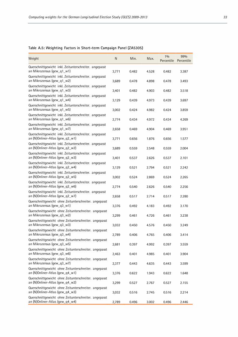
Computing weights for the German Longitudinal Election Study (GLES) 2009-2013 33
Table A.5: Weighting Factors in Short-term Campaign Panel (ZA5305)
Weight N Min. Max. 1% Percentile
99% Percentile
Querschnittgewicht inkl. Zeitunterschreiter. angepasst an Mikrozensus (gew_q1_w1) 3,771 0.482 4.528 0.482 3.387 Querschnittgewicht inkl. Zeitunterschreiter. angepasst an Mikrozensus (gew_q1_w2) 3,689 0.478 4.898 0.478 3.493 Querschnittgewicht inkl. Zeitunterschreiter. angepasst an Mikrozensus (gew_q1_w3) 3,401 0.482 4.903 0.482 3.518 Querschnittgewicht inkl. Zeitunterschreiter. angepasst an Mikrozensus (gew_q1_w4) 3,129 0.439 4.973 0.439 3.697 Querschnittgewicht inkl. Zeitunterschreiter. angepasst an Mikrozensus (gew_q1_w5) 3,002 0.424 4.982 0.424 3.859 Querschnittgewicht inkl. Zeitunterschreiter. angepasst an Mikrozensus (gew_q1_w6) 2,774 0.434 4.972 0.434 4.269 Querschnittgewicht inkl. Zeitunterschreiter. angepasst an Mikrozensus (gew_q1_w7) 2,658 0.469 4.904 0.469 3.951 Querschnittgewicht inkl. Zeitunterschreiter. angepasst an (N)Onliner-Atlas (gew_q2_w1) 3,771 0.656 1.876 0.656 1.577 Querschnittgewicht inkl. Zeitunterschreiter. angepasst an (N)Onliner-Atlas (gew_q2_w2) 3,689 0.559 2.548 0.559 2.004 Querschnittgewicht inkl. Zeitunterschreiter. angepasst an (N)Onliner-Atlas (gew_q2_w3) 3,401 0.537 2.626 0.537 2.101 Querschnittgewicht inkl. Zeitunterschreiter. angepasst an (N)Onliner-Atlas (gew_q2_w4) 3,129 0.521 2.794 0.521 2.242 Querschnittgewicht inkl. Zeitunterschreiter. angepasst an (N)Onliner-Atlas (gew_q2_w5) 3,002 0.524 2.869 0.524 2.265 Querschnittgewicht inkl. Zeitunterschreiter. angepasst an (N)Onliner-Atlas (gew_q2_w6) 2,774 0.540 2.626 0.540 2.256 Querschnittgewicht inkl. Zeitunterschreiter. angepasst an (N)Onliner-Atlas (gew_q2_w7) 2,658 0.517 2.714 0.517 2.280 Querschnittgewicht ohne Zeitunterschreiter. angepasst an Mikrozensus (gew_q3_w1) 3,376 0.492 4.183 0.492 3.170 Querschnittgewicht ohne Zeitunterschreiter. angepasst an Mikrozensus (gew_q3_w2) 3,299 0.461 4.726 0.461 3.238 Querschnittgewicht ohne Zeitunterschreiter. angepasst an Mikrozensus (gew_q3_w3) 3,032 0.450 4.576 0.450 3.249 Querschnittgewicht ohne Zeitunterschreiter. angepasst an Mikrozensus (gew_q3_w4) 2,789 0.406 4.765 0.406 3.414 Querschnittgewicht ohne Zeitunterschreiter. angepasst an Mikrozensus (gew_q3_w5) 2,681 0.397 4.992 0.397 3.559 Querschnittgewicht ohne Zeitunterschreiter. angepasst an Mikrozensus (gew_q3_w6) 2,463 0.401 4.985 0.401 3.904 Querschnittgewicht ohne Zeitunterschreiter. angepasst an Mikrozensus (gew_q3_w7) 2,377 0.443 4.635 0.443 3.599 Querschnittgewicht ohne Zeitunterschreiter. angepasst an (N)Onliner-Atlas (gew_q4_w1) 3,376 0.622 1.943 0.622 1.648 Querschnittgewicht ohne Zeitunterschreiter. angepasst an (N)Onliner-Atlas (gew_q4_w2) 3,299 0.527 2.767 0.527 2.155 Querschnittgewicht ohne Zeitunterschreiter. angepasst an (N)Onliner-Atlas (gew_q4_w3) 3,032 0.516 2.745 0.516 2.214 Querschnittgewicht ohne Zeitunterschreiter. angepasst an (N)Onliner-Atlas (gew_q4_w4) 2,789 0.496 3.002 0.496 2.446
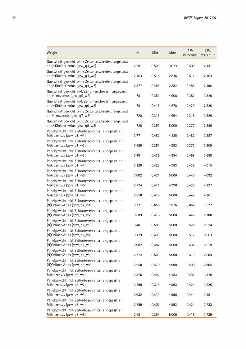
34 GESIS Papers 2017|07
Weight N Min. Max. 1%
Percentile 99%
Percentile
Querschnittgewicht ohne Zeitunterschreiter. angepasst an (N)Onliner-Atlas (gew_q4_w5) 2,681 0.500 3.023 0.500 2.431 Querschnittgewicht ohne Zeitunterschreiter. angepasst an (N)Onliner-Atlas (gew_q4_w6) 2,463 0.511 2.846 0.511 2.463 Querschnittgewicht ohne Zeitunterschreiter. angepasst an (N)Onliner-Atlas (gew_q4_w7) 2,377 0.488 2.882 0.488 2.496 Querschnittgewicht inkl. Zeitunterschreiter. angepasst an Mikrozensus (gew_q5_w2) 781 0.351 4.908 0.351 3.820 Querschnittgewicht inkl. Zeitunterschreiter. angepasst an (N)Onliner-Atlas (gew_q6_w2) 781 0.416 4.878 0.429 2.526 Querschnittgewicht ohne Zeitunterschreiter. angepasst an Mikrozensus (gew_q7_w2) 720 0.318 4.694 0.318 3.526 Querschnittgewicht ohne Zeitunterschreiter. angepasst an (N)Onliner-Atlas (gew_q8_w2) 720 0.353 5.000 0.377 2.886 Panelgewicht inkl. Zeitunterschreiter. angepasst an Mikrozensus (gew_p1_w1) 3,771 0.482 4.528 0.482 3.387 Panelgewicht inkl. Zeitunterschreiter. angepasst an Mikrozensus (gew_p1_w2) 3,689 0.351 4.992 0.373 3.809 Panelgewicht inkl. Zeitunterschreiter. angepasst an Mikrozensus (gew_p1_w3) 3,401 0.426 4.994 0.458 3.680 Panelgewicht inkl. Zeitunterschreiter. angepasst an Mikrozensus (gew_p1_w4) 3,129 0.428 4.983 0.439 4.015 Panelgewicht inkl. Zeitunterschreiter. angepasst an Mikrozensus (gew_p1_w5) 3,002 0.421 5.000 0.440 4.092 Panelgewicht inkl. Zeitunterschreiter. angepasst an Mikrozensus (gew_p1_w6) 2,774 0.411 4.990 0.429 4.327 Panelgewicht inkl. Zeitunterschreiter. angepasst an Mikrozensus (gew_p1_w7) 2,658 0.416 5.000 0.442 4.361 Panelgewicht inkl. Zeitunterschreiter. angepasst an (N)Onliner-Atlas (gew_p2_w1) 3,771 0.656 1.876 0.656 1.577 Panelgewicht inkl. Zeitunterschreiter. angepasst an (N)Onliner-Atlas (gew_p2_w2) 3,689 0.416 5.000 0.445 2.388 Panelgewicht inkl. Zeitunterschreiter. angepasst an (N)Onliner-Atlas (gew_p2_w3) 3,401 0.503 5.000 0.522 2.524 Panelgewicht inkl. Zeitunterschreiter. angepasst an (N)Onliner-Atlas (gew_p2_w4) 3,129 0.493 5.000 0.512 2.663 Panelgewicht inkl. Zeitunterschreiter. angepasst an (N)Onliner-Atlas (gew_p2_w5) 3,002 0.487 5.000 0.492 2.519 Panelgewicht inkl. Zeitunterschreiter. angepasst an (N)Onliner-Atlas (gew_p2_w6) 2,774 0.509 5.000 0.513 2.684 Panelgewicht inkl. Zeitunterschreiter. angepasst an (N)Onliner-Atlas (gew_p2_w7) 2,658 0.470 4.998 0.490 2.805 Panelgewicht inkl. Zeitunterschreiter. angepasst an Mikrozensus (gew_p3_w1) 3,376 0.492 4.183 0.492 3.170 Panelgewicht inkl. Zeitunterschreiter. angepasst an Mikrozensus (gew_p3_w2) 3,299 0.318 4.993 0.424 3.526 Panelgewicht inkl. Zeitunterschreiter. angepasst an Mikrozensus (gew_p3_w3) 3,032 0.419 4.998 0.444 3.451 Panelgewicht inkl. Zeitunterschreiter. angepasst an Mikrozensus (gew_p3_w4) 2,789 0.401 4.993 0.424 3.723 Panelgewicht inkl. Zeitunterschreiter. angepasst an Mikrozensus (gew_p3_w5) 2,681 0.391 5.000 0.415 3.739

Computing weights for the German Longitudinal Election Study (GLES) 2009-2013 35
Weight N Min. Max. 1%
Percentile 99%
Percentile
Panelgewicht inkl. Zeitunterschreiter. angepasst an Mikrozensus (gew_p3_w6) 2,463 0.375 4.998 0.404 4.159 Panelgewicht inkl. Zeitunterschreiter. angepasst an Mikrozensus (gew_p3_w7) 2,377 0.390 5.000 0.440 4.168 Panelgewicht inkl. Zeitunterschreiter. angepasst an (N)Onliner-Atlas (gew_p4_w1) 3,376 0.622 1.943 0.622 1.648 Panelgewicht inkl. Zeitunterschreiter. angepasst an (N)Onliner-Atlas (gew_p4_w2) 3,299 0.356 5.394 0.390 2.686 Panelgewicht inkl. Zeitunterschreiter. angepasst an (N)Onliner-Atlas (gew_p4_w3) 3,032 0.453 5.000 0.482 2.427 Panelgewicht inkl. Zeitunterschreiter. angepasst an (N)Onliner-Atlas (gew_p4_w4) 2,789 0.458 5.000 0.470 2.857 Panelgewicht inkl. Zeitunterschreiter. angepasst an (N)Onliner-Atlas (gew_p4_w5) 2,681 0.454 5.000 0.465 2.687 Panelgewicht inkl. Zeitunterschreiter. angepasst an (N)Onliner-Atlas (gew_p4_w6) 2,463 0.474 5.000 0.480 2.884 Panelgewicht inkl. Zeitunterschreiter. angepasst an (N)Onliner-Atlas (gew_p4_w7) 2,377 0.429 5.000 0.457 3.060 Querschnittgewicht inkl. Zeitunterschreiter. angepasst an Mikrozensus (gew_q1_ges) 1,792 0.207 5.000 0.277 5.000 Querschnittgewicht inkl. Zeitunterschreiter. angepasst an (N)Onliner-Atlas (gew_q2_ges) 1,792 0.263 4.989 0.285 2.783 Querschnittgewicht ohne Zeitunterschreiter. angepasst an Mikrozensus (gew_q3_ges) 1,594 0.162 5.000 0.217 5.000 Querschnittgewicht ohne Zeitunterschreiter. angepasst an (N)Onliner-Atlas (gew_q4_ges) 1,594 0.081 5.000 0.086 2.526 Panelgewicht inkl. Zeitunterschreiter. angepasst an Mikrozensus (gew_p1_ges) 1,792 0.155 5.000 0.244 5.000 Panelgewicht inkl. Zeitunterschreiter. angepasst an (N)Onliner-Atlas (gew_p2_ges) 1,792 0.184 5.000 0.222 3.867 Panelgewicht inkl. Zeitunterschreiter. angepasst an Mikrozensus (gew_p3_ges) 1,594 0.133 5.000 0.207 5.000 Panelgewicht inkl. Zeitunterschreiter. angepasst an (N)Onliner-Atlas (gew_p4_ges) 1,594 0.068 5.000 0.084 3.563
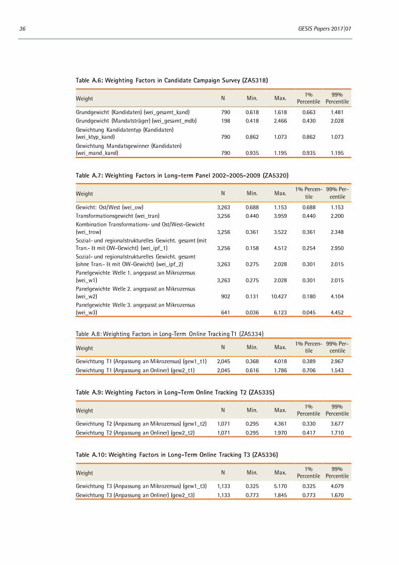
36 GESIS Papers 2017|07
Table A.6: Weighting Factors in Candidate Campaign Survey (ZA5318)
Weight N Min. Max. 1% Percentile
99% Percentile
Grundgewicht (Kandidaten) (wei_gesamt_kand) 790 0.618 1.618 0.663 1.481 Grundgewicht (Mandatsträger) (wei_gesamt_mdb) 198 0.418 2.466 0.430 2.028 Gewichtung Kandidatentyp (Kandidaten) (wei_ktyp_kand) 790 0.862 1.073 0.862 1.073 Gewichtung Mandatsgewinner (Kandidaten) (wei_mand_kand) 790 0.935 1.195 0.935 1.195
Table A.7: Weighting Factors in Long-term Panel 2002-2005-2009 (ZA5320)
Weight N Min. Max. 1% Percen-
tile 99% Per-
centile
Gewicht: Ost/West (wei_ow) 3,263 0.688 1.153 0.688 1.153 Transformationsgewicht (wei_tran) 3,256 0.440 3.959 0.440 2.200 Kombination Transformations- und Ost/West-Gewicht (wei_trow) 3,256 0.361 3.522 0.361 2.348 Sozial- und regionalstrukturelles Gewicht. gesamt (mit Tran.- & mit OW-Gewicht) (wei_ipf_1) 3,256 0.158 4.512 0.254 2.950 Sozial- und regionalstrukturelles Gewicht. gesamt (ohne Tran.- & mit OW-Gewicht) (wei_ipf_2) 3,263 0.275 2.028 0.301 2.015 Panelgewichte Welle 1. angepasst an Mikrozensus (wei_w1) 3,263 0.275 2.028 0.301 2.015 Panelgewichte Welle 2. angepasst an Mikrozensus (wei_w2) 902 0.131 10.427 0.180 4.104 Panelgewichte Welle 3. angepasst an Mikrozensus (wei_w3) 641 0.036 6.123 0.045 4.452
Table A.8: Weighting Factors in Long-Term Online Tracking T1 (ZA5334)
Weight N Min. Max. 1% Percen-tile
99% Per-centile
Gewichtung T1 (Anpassung an Mikrozensus) (gew1_t1) 2,045 0.368 4.018 0.389 2.967 Gewichtung T1 (Anpassung an Onliner) (gew2_t1) 2,045 0.616 1.786 0.706 1.543
Table A.9: Weighting Factors in Long-Term Online Tracking T2 (ZA5335)
Weight N Min. Max. 1% Percentile
99% Percentile
Gewichtung T2 (Anpassung an Mikrozensus) (gew1_t2) 1,071 0.295 4.361 0.330 3.677 Gewichtung T2 (Anpassung an Onliner) (gew2_t2) 1,071 0.295 1.970 0.417 1.710
Table A.10: Weighting Factors in Long-Term Online Tracking T3 (ZA5336)
Weight N Min. Max. 1% Percentile
99% Percentile
Gewichtung T3 (Anpassung an Mikrozensus) (gew1_t3) 1,133 0.325 5.170 0.325 4.079 Gewichtung T3 (Anpassung an Onliner) (gew2_t3) 1,133 0.773 1.845 0.773 1.670

Computing weights for the German Longitudinal Election Study (GLES) 2009-2013 37
Table A.11: Weighting Factors in Long-Term Online Tracking T4 (ZA5337)
Weight N Min. Max. 1% Percentile
99% Percentile
Gewichtung T4 (Anpassung an Mikrozensus) (gew1_t4) 1,144 0.494 3.707 0.494 3.428 Gewichtung T4 (Anpassung an Onliner) (gew2_t4) 1,144 0.762 1.362 0.762 1.362
Table A.12: Weighting Factors in Long-Term Online Tracking T5 (ZA5338)
Weight N Min. Max. 1% Percentile
99% Percentile
Gewichtung T5 (Anpassung an Mikrozensus) (gew1_t5) 1,139 0.325 3.752 0.336 3.529 Gewichtung T5 (Anpassung an Onliner) (gew2_t5) 1,139 0.623 1.498 0.715 1.498
Table A.13: Weighting Factors in Long-Term Online Tracking T6 (ZA5339)
Weight N Min. Max. 1% Percentile
99% Percentile
Gewichtung T6 (Anpassung an Mikrozensus) (gew1_t6) 1,153 0.388 3.857 0.388 2.869 Gewichtung T6 (Anpassung an Onliner) (gew2_t6) 1,153 0.683 1.741 0.713 1.527
Table A.14: Weighting Factors in Long-Term Online Tracking T7 (ZA5340)
Weight N Min. Max. 1% Percentile
99% Percentile
Gewichtung T7: Anpassung an Mikrozensus (Gesamtes Sample) (gew1_t7_v0) 1,147 0.449 3.627 0.449 3.224 Gewichtung T7: Anpassung an Onliner (Gesamtes Sample) (gew2_t7_v0) 1,147 0.160 6.549 0.160 5.385 Gewichtung T7: Anpassung an Mikrozensus (Ohne Zeitunterschreiter) (gew1_t7_v1) 1,027 0.446 3.713 0.446 3.285 Gewichtung T7: Anpassung an Onliner (Ohne Zeitun-terschreiter) (gew2_t7_v1) 1,027 0.174 6.143 0.174 5.751 Gewichtung T7: Anpassung an Mikrozensus (Ohne Zeitunterschreiter und Mutationen) (gew1_t7_v2) 928 0.443 3.659 0.443 3.151 Gewichtung T7: Anpassung an Onliner (Ohne Zeitun-terschreiter und Mutationen) (gew2_t7_v2) 928 0.167 6.140 0.167 5.865
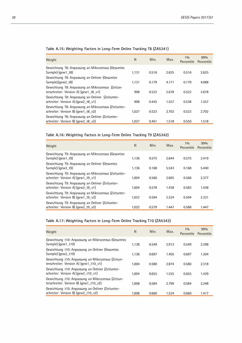
38 GESIS Papers 2017|07
Table A.15: Weighting Factors in Long-Term Online Tracking T8 (ZA5341)
Weight N Min. Max. 1% Percentile
99% Percentile
Gewichtung T8: Anpassung an Mikrozensus (Gesamtes Sample) (gew1_t8) 1,131 0.516 2.625 0.516 2.625 Gewichtung T8: Anpassung an Onliner (Gesamtes Sample).(gew2_t8) 1,131 0.179 4.171 0.179 4.088 Gewichtung T8: Anpassung an Mikrozensus (Zeitun-terschreiter: Version A) (gew1_t8_v1) 998 0.522 2.678 0.522 2.678 Gewichtung T8: Anpassung an Onliner (Zeitunter-schreiter: Version A) (gew2_t8_v1) 998 0.445 1.557 0.538 1.557 Gewichtung T8: Anpassung an Mikrozensus (Zeitunter-schreiter: Version B) (gew1_t8_v2) 1,027 0.523 2.702 0.523 2.702 Gewichtung T8: Anpassung an Onliner (Zeitunter-schreiter: Version B) (gew2_t8_v2) 1,027 0.461 1.518 0.550 1.518
Table A.16: Weighting Factors in Long-Term Online Tracking T9 (ZA5342)
Weight N Min. Max. 1% Percentile
99% Percentile
Gewichtung T9: Anpassung an Mikrozensus (Gesamtes Sample) (gew1_t9) 1,136 0.575 2.644 0.575 2.419 Gewichtung T9: Anpassung an Onliner (Gesamtes Sample) (gew2_t9) 1,136 0.168 5.543 0.168 5.440 Gewichtung T9: Anpassung an Mikrozensus (Zeitunter-schreiter: Version A) (gew1_t9_v1) 1,004 0.566 2.605 0.566 2.377 Gewichtung T9: Anpassung an Onliner (Zeitunter-schreiter: Version A) (gew2_t9_v1) 1,004 0.578 1.438 0.583 1.438 Gewichtung T9: Anpassung an Mikrozensus (Zeitunter-schreiter: Version B) (gew1_t9_v2) 1,022 0.594 2.524 0.594 2.331 Gewichtung T9: Anpassung an Onliner (Zeitunter-schreiter: Version B) (gew2_t9_v2) 1,022 0.579 1.447 0.588 1.447
Table A.17: Weighting Factors in Long-Term Online Tracking T10 (ZA5343)
Weight N Min. Max. 1%
Percentile 99%
Percentile
Gewichtung t10: Anpassung an Mikrozensus (Gesamtes Sample) (gew1_t10) 1,138 0.549 2.913 0.549 2.298 Gewichtung t10: Anpassung an Onliner (Gesamtes Sample) (gew2_t10) 1,138 0.697 1.405 0.697 1.304 Gewichtung t10: Anpassung an Mikrozensus (Zeitun-terschreiter: Version A) (gew1_t10_v1) 1,004 0.580 2.874 0.580 2.318 Gewichtung t10: Anpassung an Onliner (Zeitunter-schreiter: Version A) (gew2_t10_v1) 1,004 0.655 1.535 0.655 1.429 Gewichtung t10: Anpassung an Mikrozensus (Zeitun-terschreiter: Version B) (gew1_t10_v2) 1,008 0.584 2.799 0.584 2.248 Gewichtung t10: Anpassung an Onliner (Zeitunter-schreiter: Version B) (gew2_t10_v2) 1,008 0.660 1.524 0.660 1.417
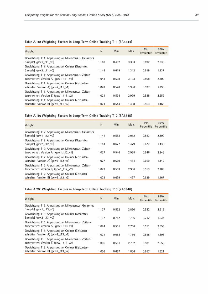
Computing weights for the German Longitudinal Election Study (GLES) 2009-2013 39
Table A.18: Weighting Factors in Long-Term Online Tracking T11 (ZA5344)
Weight N Min. Max. 1% Percentile
99% Percentile
Gewichtung T11: Anpassung an Mikrozensus (Gesamtes Sample) (gew1_t11_v0) 1,148 0.492 3.353 0.492 2.838 Gewichtung T11: Anpassung an Onliner (Gesamtes Sample) (gew2_t11_v0) 1,148 0.619 1.342 0.619 1.337 Gewichtung T11: Anpassung an Mikrozensus (Zeitun-terschreiter: Version A) (gew1_t11_v1) 1,043 0.508 3.193 0.508 2.800 Gewichtung T11: Anpassung an Onliner (Zeitunter-schreiter: Version A) (gew2_t11_v1) 1,043 0.578 1.396 0.597 1.396 Gewichtung T11: Anpassung an Mikrozensus (Zeitun-terschreiter: Version B) (gew1_t11_v2) 1,021 0.538 2.999 0.538 2.659 Gewichtung T11: Anpassung an Onliner (Zeitunter-schreiter: Version B) (gew2_t11_v2) 1,021 0.544 1.468 0.563 1.468
Table A.19: Weighting Factors in Long-Term Online Tracking T12 (ZA5345)
Weight N Min. Max. 1% Percentile
99% Percentile
Gewichtung T12: Anpassung an Mikrozensus (Gesamtes Sample) (gew1_t12_v0) 1,144 0.553 3.012 0.553 2.300 Gewichtung T12: Anpassung an Onliner (Gesamtes Sample) (gew2_t12_v0) 1,144 0.677 1.479 0.677 1.436 Gewichtung T12: Anpassung an Mikrozensus (Zeitun-terschreiter: Version A) (gew1_t12_v1) 1,027 0.546 2.968 0.546 2.246 Gewichtung T12: Anpassung an Onliner (Zeitunter-schreiter: Version A) (gew2_t12_v1) 1,027 0.669 1.454 0.669 1.442 Gewichtung T12: Anpassung an Mikrozensus (Zeitun-terschreiter: Version B) (gew1_t12_v2) 1,023 0.553 2.906 0.553 2.189 Gewichtung T12: Anpassung an Onliner (Zeitunter-schreiter: Version B) (gew2_t12_v2) 1,023 0.639 1.467 0.639 1.467
Table A.20: Weighting Factors in Long-Term Online Tracking T13 (ZA5346)
Weight N Min. Max. 1%
Percentile 99%
Percentile
Gewichtung T13: Anpassung an Mikrozensus (Gesamtes Sample) (gew1_t13_v0) 1,137 0.532 2.880 0.532 2.512 Gewichtung T13: Anpassung an Onliner (Gesamtes Sample) (gew2_t13_v0) 1,137 0.712 1.786 0.712 1.534 Gewichtung T13: Anpassung an Mikrozensus (Zeitun-terschreiter: Version A) (gew1_t13_v1) 1,024 0.551 2.756 0.551 2.553 Gewichtung T13: Anpassung an Onliner (Zeitunter-schreiter: Version A) (gew2_t13_v1) 1,024 0.658 1.756 0.658 1.608 Gewichtung T13: Anpassung an Mikrozensus (Zeitun-terschreiter: Version B) (gew1_t13_v2) 1,006 0.581 2.732 0.581 2.559 Gewichtung T13: Anpassung an Onliner (Zeitunter-schreiter: Version B) (gew2_t13_v2) 1,006 0.657 1.806 0.657 1.621

40 GESIS Papers 2017|07
Table A.21: Weighting Factors in Long-Term Online Tracking T14 (ZA5347)
Weight N Min. Max. 1% Percentile
99% Percentile
Gewichtung T14: Anpassung an Mikrozensus (Gesamtes Sample) (gew1_t14_v0) 1,150 0.457 2.709 0.457 2.384 Gewichtung T14: Anpassung an Onliner (Gesamtes Sample) (gew2_t14_v0) 1,150 0.704 1.403 0.704 1.357 Gewichtung T14: Anpassung an Mikrozensus (Zeitun-terschreiter: Version A) (gew1_t14_v1) 1,039 0.485 2.373 0.485 2.134 Gewichtung T14: Anpassung an Onliner (Zeitunter-schreiter: Version A) (gew2_t14_v1) 1,039 0.669 1.471 0.669 1.471 Gewichtung T14: Anpassung an Mikrozensus (Zeitun-terschreiter: Version B) (gew1_t14_v2) 1,039 0.494 2.312 0.494 2.096 Gewichtung T14: Anpassung an Onliner (Zeitunter-schreiter: Version B) (gew2_t14_v2) 1,039 0.646 1.551 0.646 1.551
Table A.22: Weighting Factors in Long-Term Online Tracking T15 (ZA5348)
Weight N Min. Max. 1% Percentile
99% Percentile
Gewichtung T15: Anpassung an Mikrozensus (Gesamtes Sample) (gew1_t15_v0) 1,158 0.407 2.199 0.407 2.199 Gewichtung T15: Anpassung an Onliner (Gesamtes Sample) (gew2_t15_v0) 1,158 0.467 1.604 0.526 1.604 Gewichtung T15: Anpassung an Mikrozensus (Zeitun-terschreiter: Version A) (gew1_t15_v1) 1,020 0.438 2.007 0.438 2.007 Gewichtung T15: Anpassung an Onliner (Zeitunter-schreiter: Version A) (gew2_t15_v1) 1,020 0.408 1.616 0.480 1.616 Gewichtung T15: Anpassung an Mikrozensus (Zeitun-terschreiter: Version B) (gew1_t15_v2) 1,028 0.438 1.978 0.438 1.978 Gewichtung T15: Anpassung an Onliner (Zeitunter-schreiter: Version B) (gew2_t15_v2) 1,028 0.419 1.584 0.475 1.583
Table A.23: Weighting Factors in Long-Term Online Tracking T16 (ZA5349)
Weight N Min. Max. 1%
Percentile 99%
Percentile
Gewichtung Welle T16 (Anpassung an Mikrozensus) (Version Z) (gew1_t16_v0) 1,114 0.481 3.435 0.481 2.916 Gewichtung Welle T16 (Anpassung an Onliner) (Version Z) (gew2_t16_v0) 1,114 0.794 1.355 0.794 1.319 Gewichtung Welle T16 (Anpassung an Mikrozensus) (Version A) (gew1_t16_v1) 994 0.497 3.360 0.497 2.826 Gewichtung Welle T16 (Anpassung an Onliner) (Version A) (gew2_t16_v1) 994 0.782 1.339 0.782 1.339 Gewichtung Welle T16 (Anpassung an Mikrozensus) (Version B) (gew1_t16_v2) 999 0.498 3.206 0.498 2.740 Gewichtung Welle T16 (Anpassung an Onliner) (Version B) (gew2_t16_v2) 999 0.777 1.365 0.777 1.365

Computing weights for the German Longitudinal Election Study (GLES) 2009-2013 41
Table A.24: Weighting Factors in Long-Term Online Tracking T17 (ZA5350)
Weight N Min. Max. 1% Percentile
99% Percentile
Sozial- und regionalstrukt Gewicht (Anpassung MZ2009. mit Zeitunterschreiter) (wei_mzz) 1,016 0.536 3.328 0.539 2.746 Sozial- und regionalstrukt Gewicht (Anpassung MZ2009. ohne Zeitunterschreiter) (wei_mzoz) 914 0.563 3.018 0.573 2.467 Sozial- und regionalstrukt Gewicht (Anpassung Onli-ner. mit Zeitunterschreiter) (wei_onz) 1,016 0.112 5.648 0.112 5.648 Sozial- und regionalstrukt Gewicht (Anpassung Onli-ner. ohne Zeitunterschreiter (wei_onoz) 914 0.079 5.490 0.079 5.490
Table A.25: Weighting Factors in Long-Term Online Tracking T18 (ZA5351)
Weight N Min. Max. 1% Percentile
99% Percentile
Sozial- und regionalstrukturelles Gewicht (Anpassung MZ2009. mit Zeitunterschreiter) (wei_mzz) 1,075 0.497 3.435 0.497 2.621 Sozial- und regionalstrukturelles Gewicht (Anpassung MZ2009. ohne Zeitunterschreiter) (wei_mzoz) 967 0.521 2.954 0.521 2.453 Sozial- und regionalstrukturelles Gewicht (Anpassung Onliner. mit Zeitunterschreiter) (wei_onz) 1,075 0.603 1.505 0.618 1.390 Sozial- und regionalstrukturelles Gewicht (Anpassung Onliner. ohne Zeitunterschreiter) (wei_onoz) 967 0.657 1.403 0.671 1.381
Table A.26: Weighting Factors in Long-Term Online Tracking T19 (ZA5719)
Weight N Min. Max. 1%
Percentile 99%
Percentile
Sozial- und regionalstrukturelles Gewicht (Anpassung MZ2009. mit Zeitunterschreiter) (wei_mzz) 1,034 0.386 5.000 0.386 3.720 Sozial- und regionalstrukturelles Gewicht (Anpassung MZ2009. ohne Zeitunterschreiter) (wei_mzoz) 930 0.388 4.943 0.388 3.378 Sozial- und regionalstrukturelles Gewicht (Anpassung ONLINER. mit Zeitunterschreiter) (wei_onz) 1,034 0.575 1.794 0.618 1.643 Sozial- und regionalstrukturelles Gewicht (Anpassung ONLINER. ohne Zeitunterschreiter) (wei_onoz) 930 0.594 1.666 0.628 1.576 Table A.27: Weighting Factors in Long-Term Online Tracking T20 (ZA5720)
Weight N Min. Max. 1% Percentile
99% Percentile
Sozial- und regionalstrukturelles Gewicht (Anpassung MZ2009. mit Zeitunterschreiter) (wei_mzz) 1,048 0.378 3.813 0.392 3.455 Sozial- und regionalstrukturelles Gewicht (Anpassung MZ2009. ohne Zeitunterschreiter) (wei_mzoz) 943 0.396 3.499 0.412 3.115 Sozial- und regionalstrukturelles Gewicht (Anpassung ONLINER. mit Zeitunterschreiter) (wei_onz) 1,048 0.591 1.475 0.610 1.390 Sozial- und regionalstrukturelles Gewicht (Anpassung ONLINER. ohne Zeitunterschreiter) (wei_onoz) 943 0.678 1.316 0.678 1.302

42 GESIS Papers 2017|07
Table A.28: Weighting Factors in Long-Term Online Tracking T21 (ZA5721)
Weight N Min. Max. 1% Percentile
99% Percentile
Sozial- und regionalstrukturelles Gewicht (Anpassung MZ2012. mit Zeitunterschreiter) (wei_mzz) 1,012 0.339 4.113 0.373 3.481 Sozial- und regionalstrukturelles Gewicht (Anpassung MZ2012. ohne Zeitunterschreiter) (wei_mzoz) 910 0.403 3.525 0.415 2.972 Sozial- und regionalstrukturelles Gewicht (Anpassung ONLINER. mit Zeitunterschreiter) (wei_onz) 1,012 0.558 1.788 0.581 1.576 Sozial- und regionalstrukturelles Gewicht (Anpassung ONLINER. ohne Zeitunterschreiter) (wei_onoz) 910 0.715 1.403 0.715 1.344 Table A.29: Weighting Factors in Long-Term Online Tracking of State Election North Rhine-Westphalia 2010 (ZA5324)
Weight N Min. Max. 1%
Percentile 99%
Percentile
Anpassung an Mikrozensus (Gesamtes Sample) (gew1_nrw) 572 0.360 2.635 0.360 2.635 Anpassung an Onliner (Gesamtes Sample) (gew2_nrw) 572 0.454 1.959 0.454 1.824 Anpassung an Mikrozensus (Zeitunterschreiter: Version A) (gew1_nrw_v1) 512 0.388 2.505 0.388 2.505 Anpassung an Onliner (Zeitunterschreiter: Version A) (gew2_nrw_v1) 512 0.436 1.853 0.436 1.853 Anpassung an Mikrozensus (Zeitunterschreiter: Version B) (gew1_nrw_v2) 520 0.387 2.437 0.387 2.437 Anpassung an Onliner (Zeitunterschreiter: Version B) (gew2_nrw_v2) 520 0.449 1.847 0.449 1.847
Table A.30: Weighting Factors in Long-Term Online Tracking of State Election Saxony-Anhalt 2011 (ZA5325)
Weight N Min. Max. 1% Percentile
99% Percentile
Anpassung an Mikrozensus (Version Z) 580 0.391 6.508 0.391 6.508 Anpassung an Onliner (Version Z) (gew2_st_v0) 580 0.540 2.033 0.540 1.781 Anpassung an Mikrozensus (Version A) (gew1_st_v1) 516 0.412 6.621 0.412 6.621 Anpassung an Onliner (Version A) (gew2_st_v1) 516 0.478 2.087 0.478 2.009 Anpassung an Mikrozensus (Version B) (gew1_st_v2) 529 0.401 6.682 0.401 6.608 Anpassung an Onliner (Version B) (gew2_st_v2) 529 0.481 2.095 0.481 1.992
Table A.31: Weighting Factors in Long-Term Online Tracking of State Election Bremen 2011 (ZA5326)
Weight N Min. Max. 1%
Percentile 99%
Percentile
Anpassung an Mikrozensus (Version Z) (gew1_hb_v0) 510 0.380 5.211 0.380 5.211 Anpassung an Onliner (Version Z) (gew2_hb_v0) 510 0.429 2.882 0.429 2.882 Anpassung an Mikrozensus (Version A) (gew1_hb_v1) 453 0.373 4.839 0.373 4.839 Anpassung an Onliner (Version A) (gew2_hb_v1) 453 0.411 2.793 0.411 2.793 Anpassung an Mikrozensus (Version B) (gew1_hb_v2) 466 0.366 4.843 0.366 4.843 Anpassung an Onliner (Version B) (gew2_hb_v2) 466 0.385 2.910 0.385 2.910

Computing weights for the German Longitudinal Election Study (GLES) 2009-2013 43
Table A.32: Weighting Factors in Long-Term Online Tracking of State Election Rhineland-Palatinate 2011 (ZA5327)
Weight N Min. Max. 1% Percentile
99% Percentile
Anpassung an Mikrozensus (Version Z) (gew1_rp_v0) 565 0.426 2.734 0.426 2.734 Anpassung an Onliner (Version Z) (gew2_rp_v0) 565 0.588 1.412 0.588 1.412 Anpassung an Mikrozensus (Version A) (gew1_rp_v1) 509 0.419 2.630 0.419 2.630 Anpassung an Onliner (Version A) (gew2_rp_v1) 509 0.519 1.626 0.519 1.540 Anpassung an Mikrozensus (Version B) (gew1_rp_v2) 528 0.438 2.571 0.438 2.571 Anpassung an Onliner (Version B) (gew2_rp_v2) 528 0.539 1.541 0.539 1.500
Table A.33: Weighting Factors in Long-Term Online Tracking of State Election Baden-Wuerttemberg 2011 (ZA5328)
Weight N Min. Max. 1%
Percentile 99%
Percentile
Anpassung an Mikrozensus (Version Z) (gew1_bw_v0) 562 0.489 2.275 0.489 2.275 Anpassung an Onliner (Version Z) (gew2_bw_v0) 562 0.640 1.484 0.663 1.484 Anpassung an Mikrozensus (Version A) (gew1_bw_v1) 494 0.499 2.174 0.499 2.174 Anpassung an Onliner (Version A) (gew2_bw_v1) 494 0.566 1.532 0.566 1.532 Anpassung an Mikrozensus (Version B) (gew1_bw_v2) 495 0.515 2.123 0.515 2.123 Anpassung an Onliner (Version B) (gew2_bw_v2) 495 0.575 1.531 0.575 1.531
Table A.34: Weighting Factors in Long-Term Online Tracking of State Election Berlin 2011 (ZA5329)
Weight N Min. Max. 1% Percentile
99% Percentile
Gewichtung BE (Anpassung an Mikrozensus) (Version Z) (gew1_be_v0) 615 0.611 2.183 0.611 2.183 Gewichtung BE (Anpassung an Onliner) (Version Z) (gew2_be_v0) 615 0.437 2.268 0.437 2.097 Gewichtung BE (Anpassung an Mikrozensus) (Version A) (gew1_be_v1) 531 0.645 1.877 0.645 1.877 Gewichtung BE (Anpassung an Onliner) (Version A) (gew2_be_v1) 531 0.437 2.284 0.437 2.284 Gewichtung BE (Anpassung an Mikrozensus) (Version B) (gew1_be_v2) 555 0.644 2.024 0.644 2.024 Gewichtung BE (Anpassung an Onliner) (Version B) (gew2_be_v2) 555 0.426 2.298 0.426 2.298

44 GESIS Papers 2017|07
Table A.35: Weighting Factors in Long-Term Online Tracking of State Election Berlin 2011 (ZA5330)
Weight N Min. Max. 1% Percentile
99% Percentile
Anpassung an Mikrozensus (Version Z) (gew1_mv_v0) 562 0.310 4.306 0.310 4.306 Anpassung an Onliner (Version Z) (gew2_mv_v0) 562 0.474 1.754 0.474 1.754 Anpassung an Mikrozensus (Version A) (gew1_mv_v1) 493 0.347 4.210 0.347 4.210 Anpassung an Onliner (Version A) (gew2_mv_v1) 493 0.381 2.008 0.381 2.008 Anpassung an Mikrozensus (Version B) (gew1_mv_v2) 516 0.337 4.041 0.337 4.041 Gewichtung MV (Anpassung an Onliner) (Version B) (gew2_mv_v2) 516 0.401 1.886 0.401 1.886
Table A.36: Weighting Factors in Long-Term Online Tracking of State Election Hamburg 2011 (ZA5331)
Weight N Min. Max. 1% Percentile
99% Percentile
Anpassung an Mikrozensus (Version Z) (gew1_hh_v0) 538 0.528 2.689 0.528 2.689 Anpassung an Onliner (Version Z) (gew2_hh_v0) 538 0.512 1.821 0.512 1.821 Anpassung an Mikrozensus (Version A) (gew1_hh_v1) 475 0.534 2.274 0.534 2.274 Anpassung an Onliner (Version A) (gew2_hh_v1) 475 0.461 2.006 0.461 2.006 Anpassung an Mikrozensus (Version B) (gew1_hh_v2) 490 0.538 2.461 0.538 2.461 Anpassung an Onliner (Version B) (gew2_hh_v2) 490 0.483 2.094 0.483 2.094 Table A.37: Weighting Factors in Long-Term Online Tracking of State Election Lower Saxony 2013 (ZA5735)
Weight N Min. Max. 1% Percentile
99% Percentile
Sozial- und regionalstrukturelles Gewicht (MZ2009. mit Zeitunterschreiter) (wei_mzz) 543 0.229 5.000 0.229 5.000 Sozial- und regionalstrukturelles Gewicht (MZ2009. ohne Zeitunterschreiter) (wei_mzoz) 488 0.234 5.000 0.234 5.000 Sozial- und regionalstrukturelles Gewicht (Onliner. mit Zeitunterschreiter) (wei_onz) 543 0.569 2.196 0.631 2.004 Sozial- und regionalstrukturelles Gewicht (Onliner. ohne Zeitunterschreiter) (wei_onoz) 488 0.519 2.102 0.564 2.102
Table A.38: Weighting Factors in Long-Term Online Tracking of State Election Bavaria 2013 (ZA5736)
Weight N Min. Max. 1%
Percentile 99%
Percentile
Sozial- und regionalstrukturelles Gewicht (Anpassung MZ2009. mit Zeitunterschreiter) (wei_mzzob) 532 0.380 3.323 0.380 3.323 Sozial- und regionalstrukturelles Gewicht (Anpassung MZ2009. ohne Zeitunterschreiter) (wei_mzozob) 478 0.399 2.981 0.399 2.981 Sozial- und regionalstrukturelles Gewicht (Anpassung Onliner. mit Zeitunterschreiter) (wei_onz) 532 0.285 1.948 0.285 1.948 Sozial- und regionalstrukturelles Gewicht (Anpassung Onliner. ohne Zeitunterschreiter) (wei_onoz) 478 0.281 2.177 0.281 2.177

Computing weights for the German Longitudinal Election Study (GLES) 2009-2013 45
Table A.39: Weighting Factors in Long-Term Online Tracking of State Election Hesse 2013 (ZA5737)
Weight N Min. Max. 1% Percentile
99% Percentile
Sozial- und regionalstrukturelles Gewicht (Anpassung MZ2009. mit Zeitunterschreiter) (wei_mzz) 529 0.153 5.000 0.153 5.000 Sozial- und regionalstrukturelles Gewicht (Anpassung MZ2009. ohne Zeitunterschreiter) (wei_mzoz) 476 0.155 5.000 0.155 5.000 Sozial- und regionalstrukturelles Gewicht (Anpassung Onliner. mit Zeitunterschreiter) (wei_onz) 529 0.601 1.911 0.609 1.911 Sozial- und regionalstrukturelles Gewicht (Anpassung Onliner. ohne Zeitunterschreiter) (wei_onoz) 476 0.566 1.830 0.585 1.830
Table A.40: Weighting Factors in Pre-Election Cross Section (ZA5700)
Weight N Min. Max. 1% Percentile
99% Percentile
Ost-/West Gewicht (w_ow) 2,003 0.558 1.266 0.558 1.266 Transformationsgewicht (w_tran) 2,003 0.565 3.391 0.565 2.351 Kombination Transformations- und Ost/West-Gewicht (w_trow) 2,003 0.328 4.293 0.328 2.862 Sozial- und regionalstrukturelles Gewicht. gesamt (mit Tran.- & mit OW-Gewicht) (w_ipfges_1) 2,003 0.172 5.000 0.210 3.583 Sozial- und regionalstrukturelles Gewicht. gesamt (ohne Tran.- & mit OW-Gewicht) (w_ipfges_2) 2,003 0.260 2.487 0.289 2.203 Sozial- und regionalstrukturelles Gewicht. Ost (mit Transformationsgewicht) (w_ipfost_1) 753 0.332 4.223 0.332 2.814 Sozial- und regionalstrukturelles Gewicht. Ost (ohne Transformationsgewicht) (w_ipfost_2) 753 0.523 2.099 0.523 1.839 Sozial- und regionalstrukturelles Gewicht. West (mit Transformationsgewicht) (w_ipfwes_1) 1,250 0.261 4.910 0.293 3.307 Sozial- und regionalstrukturelles Gewicht. West (ohne Transformationsgewicht)(w_ipfwes_2) 1,250 0.410 2.151 0.410 1.974
Table A.41: Weighting Factors in Post-Election Cross Section (ZA5701)
Weight N Min. Max. 1%
Percentile 99%
Percentile
Ost-/West Gewicht (w_ow) 1,908 0.545 1.284 0.545 1.284 Transformationsgewicht (w_tran) 1,908 0.552 2.758 0.552 2.308 Kombination Transformations- und Ost/West-Gewicht (w_trow) 1,908 0.315 3.542 0.315 2.834
Sozial- und regionalstrukturelles Gewicht. gesamt (mit Tran.- & mit OW) (w_ipfges_1) 1,908 0.181 4.881 0.195 3.705
Sozial- und regionalstrukturelles Gewicht. gesamt (ohne Tran.- & mit OW) (w_ipfges_2) 1,908 0.297 2.761 0.307 2.662
Sozial- und regionalstrukturelles Gewicht. Ost (mit Transformationsgewicht) (w_ipfost_1) 734 0.342 3.887 0.354 3.296
Sozial- und regionalstrukturelles Gewicht. Ost (ohne Transformationsgewicht) (w_ipfost_2) 734 0.534 2.282 0.534 2.282
Sozial- und regionalstrukturelles Gewicht. West (mit Transformationsgewicht) (w_ipfwes_1) 1,174 0.290 4.377 0.311 3.417
Sozial- und regionalstrukturelles Gewicht. West (ohne Transformationsgewicht)(w_ipfwes_2) 1,174 0.496 2.273 0.496 2.177
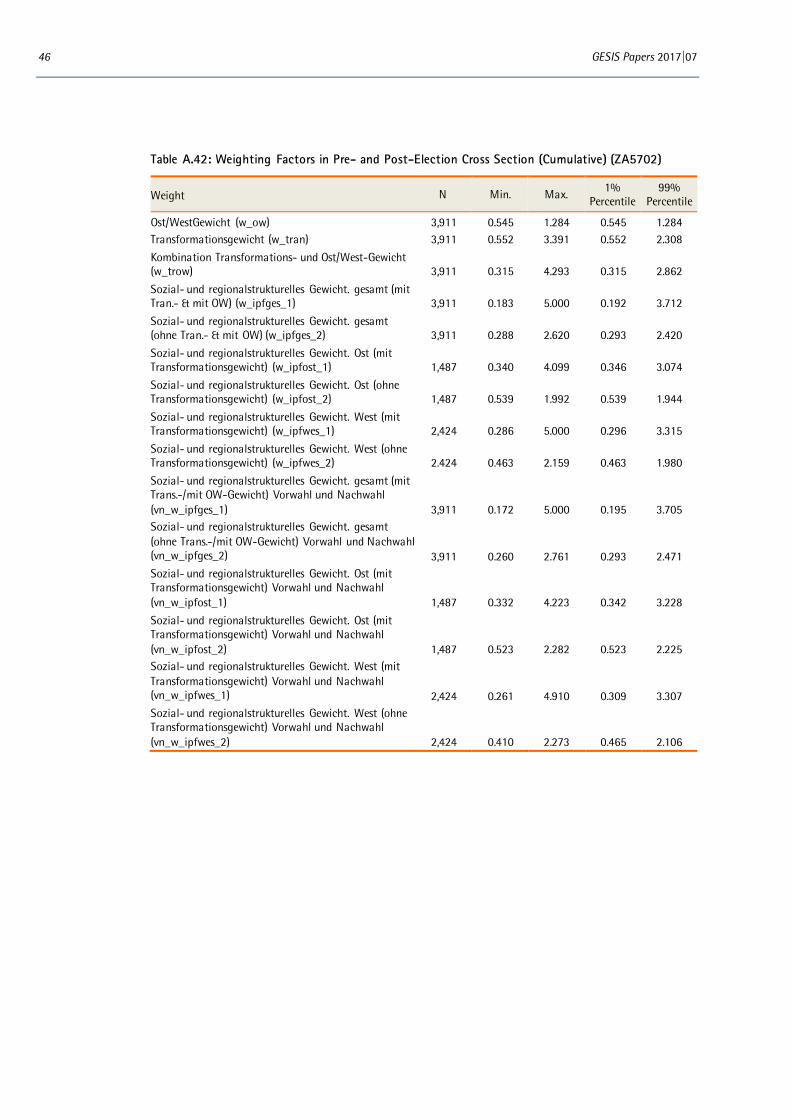
46 GESIS Papers 2017|07
Table A.42: Weighting Factors in Pre- and Post-Election Cross Section (Cumulative) (ZA5702)
Weight N Min. Max. 1% Percentile
99% Percentile
Ost/WestGewicht (w_ow) 3,911 0.545 1.284 0.545 1.284 Transformationsgewicht (w_tran) 3,911 0.552 3.391 0.552 2.308 Kombination Transformations- und Ost/West-Gewicht (w_trow) 3,911 0.315 4.293 0.315 2.862 Sozial- und regionalstrukturelles Gewicht. gesamt (mit Tran.- & mit OW) (w_ipfges_1) 3,911 0.183 5.000 0.192 3.712 Sozial- und regionalstrukturelles Gewicht. gesamt (ohne Tran.- & mit OW) (w_ipfges_2) 3,911 0.288 2.620 0.293 2.420 Sozial- und regionalstrukturelles Gewicht. Ost (mit Transformationsgewicht) (w_ipfost_1) 1,487 0.340 4.099 0.346 3.074 Sozial- und regionalstrukturelles Gewicht. Ost (ohne Transformationsgewicht) (w_ipfost_2) 1,487 0.539 1.992 0.539 1.944 Sozial- und regionalstrukturelles Gewicht. West (mit Transformationsgewicht) (w_ipfwes_1) 2,424 0.286 5.000 0.296 3.315 Sozial- und regionalstrukturelles Gewicht. West (ohne Transformationsgewicht) (w_ipfwes_2) 2.424 0.463 2.159 0.463 1.980 Sozial- und regionalstrukturelles Gewicht. gesamt (mit Trans.-/mit OW-Gewicht) Vorwahl und Nachwahl (vn_w_ipfges_1) 3,911 0.172 5.000 0.195 3.705 Sozial- und regionalstrukturelles Gewicht. gesamt (ohne Trans.-/mit OW-Gewicht) Vorwahl und Nachwahl (vn_w_ipfges_2) 3,911 0.260 2.761 0.293 2.471 Sozial- und regionalstrukturelles Gewicht. Ost (mit Transformationsgewicht) Vorwahl und Nachwahl (vn_w_ipfost_1) 1,487 0.332 4.223 0.342 3.228 Sozial- und regionalstrukturelles Gewicht. Ost (mit Transformationsgewicht) Vorwahl und Nachwahl (vn_w_ipfost_2) 1,487 0.523 2.282 0.523 2.225 Sozial- und regionalstrukturelles Gewicht. West (mit Transformationsgewicht) Vorwahl und Nachwahl (vn_w_ipfwes_1) 2,424 0.261 4.910 0.309 3.307 Sozial- und regionalstrukturelles Gewicht. West (ohne Transformationsgewicht) Vorwahl und Nachwahl (vn_w_ipfwes_2) 2,424 0.410 2.273 0.465 2.106

Computing weights for the German Longitudinal Election Study (GLES) 2009-2013 47
Table A.43: Weighting Factors Rolling Cross-Section Campaign Survey (ZA5703)
Weight N Min. Max. 1% Percentile
99% Percentile
Transformationsgewicht (gesamt) (w-trang) 7,882 0.063 7.540 0.209 2.513 Transformationsgewicht (Woche) (w_tranw) 7,882 0.062 7.515 0.207 2.532 Transformationsgewicht (Tag) (w_trant) 7,882 0.060 7.395 0.194 2.599 Bildungsgewicht mit Transformationsgewicht (gesamt) (w_bil1g) 7,882 0.038 5.000 0.126 3.420 Bildungsgewicht ohne Transformationsgewicht (ge-samt) (w_bil2g) 7,882 0.584 1.395 0.584 1.395 Bildungsgewicht mit Transformationsgewicht (Woche) (w_bil1w) 7,882 0.038 5.000 0.124 3.422 Bildungsgewicht ohne Transformationsgewicht (Wo-che) (w_bil2w) 7,882 0.562 1.448 0.562 1.448 Bildungsgewicht mit Transformationsgewicht (Tag) (w_bil1t) 7,882 0.036 5.000 0.119 3.305 Bildungsgewicht ohne Transformationsgewicht (Tag) (w_bil2t) 7,882 0.479 1.760 0.481 1.728 Soziodemographisches Gewicht mit Transformations-gewicht (gesamt) (w_soz1g) 7,882 0.031 5.000 0.129 3.607 Soziodemographisches Gewicht ohne Transformations-gewicht (gesamt) (w_soz2g) 7.882 0.436 1.675 0.436 1.675 Soziodemographisches Gewicht mit Transformations-gewicht (Woche) (w_soz1w) 7,882 0.029 5.000 0.121 3.610 Soziodemographisches Gewicht ohne Transformations-gewicht (Woche) (w_soz2w) 7,882 0.386 1.860 0.407 1.860 Sozial- und regionalstrukturelles Gewicht mit Trans-formationsgewicht (gesamt) (w_ipf1g) 7,882 0.024 5.000 0.094 4.727 Sozial- und regionalstrukturelles Gewicht ohne Trans-formationsgewicht (gesamt) (w_ipf2g) 7,882 0.348 5.000 0.348 3.676 Sozial- und regionalstrukturelles Gewicht mit Trans-formationsgewicht (Woche) (w_ipf1w) 7,882 0.023 5.000 0.093 4.799 Sozial- und regionalstrukturelles Gewicht ohne Trans-formationsgewicht (Woche) (w_ipf2w) 7,882 0.267 5.000 0.297 3.948 Panelgewicht mit Transformationsgewicht (gesamt) (w_panel1) 5,353 0.763 4.868 0.787 1.819 Panelgewicht ohne Transformationsgewicht (gesamt) (w_panel2) 5,353 0.760 5.303 0.783 1.835

48 GESIS Papers 2017|07
Table A.44: Weighting Factors in Short-Term Campaign Panel 2013 (ZA5704)
Weight N Min. Max. 1% Percentile
99% Percentile
Sozial- und regionalstrukturelles Querschnittsgewicht (Anpassung MZ2012) (wei_mz) 5,256 0.605 3.649 0.605 3.504 Sozial- und regionalstrukturelles Querschnittsgewicht (Anpassung Onliner) (wei_on) 5,256 0.710 1.671 0.710 1.671 Panelgewicht (Welle 2) (wei_w2) 4,598 0.884 2.897 0.894 1.513 Panelgewicht (Welle 3) (wei_w3) 4,432 0.931 1.645 0.935 1.168 Panelgewicht (Welle 4) (wei_w4) 4,355 0.949 2.188 0.954 1.322 Panelgewicht (Welle 5) (wei_w5) 4,257 0.944 4.125 0.951 1.310 Panelgewicht (Welle 6) (wei_w6) 4,112 0.944 3.136 0.950 1.398 Panelgewicht (Welle 7) (wei_w7) 4,231 0.969 2.781 0.972 1.219
Table A.45: Weighting Factors in Candidate Campaign Survey 2013 (ZA5716)
Weight N Min. Max. 1% Percentile
99% Percentile
Grundgewicht (Kandidaten) (wei_kandi) 1,137 0.659 1.895 0.661 1.591 Grundgewicht (Mandatsträger) (wei_mdb) 232 0.520 1.714 0.631 1.648
Table A.46: Weighting Factors in Long-Term Panel 2005-2009-2013 (ZA5321)
Weight N Min. Max. 1%
Percentile 99%
Percentile
Gewicht: Ost/West (wei_ow) 2,540 0.625 1.198 0.625 1.198 Sozial-/regionalstrukturelles Gewicht (wei_ipf) 2,540 0.338 4.728 0.338 3.984 Transformationsgewicht (wei_tran) 2,540 0.425 4.141 0.425 2.553 Panelgewicht. mit Transformationsgewicht (fwei_panel1) 686 0.442 12.298 0.478 4.675 Panelgewicht. ohne Transformationsgewicht (fwei_panel2) 686 0.451 7.543 0.485 3.951 Panelgewicht. mit Transformationsgewicht (jwei_panel1) 491 0.632 5.048 0.662 3.085 Panelgewicht. ohne Transformationsgewicht (jwei_panel2) 491 0.649 5.051 0.680 3.010
Table A.47: Weighting Factors in Long-Term Panel 2009-2013-2017 (ZA5322)
Weight N Min. Max. 1%
Percentile 99%
Percentile
Gewicht: Ost/West (wei_ow) 4,974 0.608 1.217 0.608 1.217 Transformationsgewicht (wei_tran) 4,974 0.544 3.263 0.544 2.236 Sozial- & regional. Gewicht. Gesamt (mit
Transformationsgewicht) (wei_ipfges_1) 4,974 0.205 4.827 0.24 2.967 Sozial- & regional. Gewicht. Gesamt (ohne Transformationsgewicht) (wei_ipfges_2) 4,974 0.387 1.713 0.411 1.713 Panelgewicht. mit Transformationsgewicht (jwei_panel1) 1,162 0.382 11.923 0.420 3.617 Panelgewicht. ohne Transformationsgewicht (jwei_panel2) 1,162 0.393 11.636 0.429 3.573
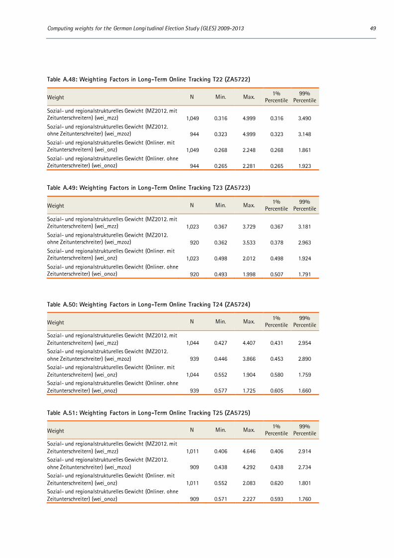
Computing weights for the German Longitudinal Election Study (GLES) 2009-2013 49
Table A.48: Weighting Factors in Long-Term Online Tracking T22 (ZA5722)
Weight N Min. Max. 1% Percentile
99% Percentile
Sozial- und regionalstrukturelles Gewicht (MZ2012. mit Zeitunterschreitern) (wei_mzz) 1,049 0.316 4.999 0.316 3.490 Sozial- und regionalstrukturelles Gewicht (MZ2012. ohne Zeitunterschreiter) (wei_mzoz) 944 0.323 4.999 0.323 3.148 Sozial- und regionalstrukturelles Gewicht (Onliner. mit Zeitunterschreitern) (wei_onz) 1,049 0.268 2.248 0.268 1.861 Sozial- und regionalstrukturelles Gewicht (Onliner. ohne Zeitunterschreiter) (wei_onoz) 944 0.265 2.281 0.265 1.923
Table A.49: Weighting Factors in Long-Term Online Tracking T23 (ZA5723)
Weight N Min. Max. 1% Percentile
99% Percentile
Sozial- und regionalstrukturelles Gewicht (MZ2012. mit Zeitunterschreitern) (wei_mzz) 1,023 0.367 3.729 0.367 3.181 Sozial- und regionalstrukturelles Gewicht (MZ2012. ohne Zeitunterschreiter) (wei_mzoz) 920 0.362 3.533 0.378 2.963 Sozial- und regionalstrukturelles Gewicht (Onliner. mit Zeitunterschreitern) (wei_onz) 1,023 0.498 2.012 0.498 1.924 Sozial- und regionalstrukturelles Gewicht (Onliner. ohne Zeitunterschreiter) (wei_onoz) 920 0.493 1.998 0.507 1.791
Table A.50: Weighting Factors in Long-Term Online Tracking T24 (ZA5724)
Weight N Min. Max. 1% Percentile
99% Percentile
Sozial- und regionalstrukturelles Gewicht (MZ2012. mit Zeitunterschreitern) (wei_mzz) 1,044 0.427 4.407 0.431 2.954 Sozial- und regionalstrukturelles Gewicht (MZ2012. ohne Zeitunterschreiter) (wei_mzoz) 939 0.446 3.866 0.453 2.890 Sozial- und regionalstrukturelles Gewicht (Onliner. mit Zeitunterschreitern) (wei_onz) 1,044 0.552 1.904 0.580 1.759 Sozial- und regionalstrukturelles Gewicht (Onliner. ohne Zeitunterschreiter) (wei_onoz) 939 0.577 1.725 0.605 1.660
Table A.51: Weighting Factors in Long-Term Online Tracking T25 (ZA5725)
Weight N Min. Max. 1% Percentile
99% Percentile
Sozial- und regionalstrukturelles Gewicht (MZ2012. mit Zeitunterschreitern) (wei_mzz) 1,011 0.406 4.646 0.406 2.914 Sozial- und regionalstrukturelles Gewicht (MZ2012. ohne Zeitunterschreiter) (wei_mzoz) 909 0.438 4.292 0.438 2.734 Sozial- und regionalstrukturelles Gewicht (Onliner. mit Zeitunterschreitern) (wei_onz) 1,011 0.552 2.083 0.620 1.801 Sozial- und regionalstrukturelles Gewicht (Onliner. ohne Zeitunterschreiter) (wei_onoz) 909 0.571 2.227 0.593 1.760

50 GESIS Papers 2017|07
Table A.52: Weighting Factors in Long-Term Online Tracking T26 (ZA5726)
Weight N Min. Max. 1% Percentile
99% Percentile
Sozial- und regionalstrukturelles Gewicht (MZ2012. mit Zeitunterschreitern) (wei_mzz) 1,019 0.409 4.718 0.409 3.611 Sozial- und regionalstrukturelles Gewicht (MZ2012. ohne Zeitunterschreiter) (wei_mzoz) 917 0.428 4.701 0.428 3.552 Sozial- und regionalstrukturelles Gewicht (Onliner. mit Zeitunterschreitern) (wei_onz) 1,019 0.637 1.965 0.637 1.813 Sozial- und regionalstrukturelles Gewicht (Onliner. ohne Zeitunterschreiter) (wei_onoz) 917 0.687 1.958 0.687 1.872
Table A.53: Weighting Factors in Long-Term Online Tracking T27 (ZA5727)
Weight N Min. Max. 1% Percentile
99% Percentile
Sozial- und regionalstrukturelles Gewicht (MZ2012. mit Zeitunterschreitern) (wei_mzz) 1,029 0.404 3.635 0.404 2.919 Sozial- und regionalstrukturelles Gewicht (MZ2012. ohne Zeitunterschreiter) (wei_mzoz) 926 0.431 3.468 0.431 2.701 Sozial- und regionalstrukturelles Gewicht (Onliner. mit Zeitunterschreitern) (wei_onz) 1,029 0.591 1.909 0.606 1.708 Sozial- und regionalstrukturelles Gewicht (Onliner. ohne Zeitunterschreiter) (wei_onoz) 926 0.641 1.730 0.649 1.580
Table A.54: Weighting Factors in Long-Term Online Tracking T28 (ZA5728)
Weight N Min. Max. 1% Percentile
99% Percentile
Sozial- und regionalstrukturelles Gewicht (MZ2012. mit Zeitunterschreitern) (wei_mzz) 1,019 0.456 4.410 0.456 3.153 Sozial- und regionalstrukturelles Gewicht (MZ2012. ohne Zeitunterschreiter) (wei_mzoz) 917 0.416 4.260 0.416 2.926 Sozial- und regionalstrukturelles Gewicht (Onliner. mit Zeitunterschreitern) (wei_onz) 1,019 0.784 1.674 0.784 1.537 Sozial- und regionalstrukturelles Gewicht (Onliner. ohne Zeitunterschreiter) (wei_onoz) 917 0.689 1.981 0.689 1.716
Table A.55: Weighting Factors in Long-Term Online Tracking T29 (ZA5729)
Weight N Min. Max. 1% Percentile
99% Percentile
Sozial- und regionalstrukturelles Gewicht (MZ2012. mit Zeitunterschreitern) (wei_mzz) 1,027 0.528 3.362 0.528 2.875 Sozial- und regionalstrukturelles Gewicht (MZ2012. ohne Zeitunterschreiter) (wei_mzoz) 924 0.506 3.080 0.506 2.737 Sozial- und regionalstrukturelles Gewicht (Onliner. mit Zeitunterschreitern) (wei_onz) 1,027 0.796 1.529 0.796 1.443 Sozial- und regionalstrukturelles Gewicht (Onliner. ohne Zeitunterschreiter) (wei_onoz) 924 0.699 1.648 0.699 1.552

Computing weights for the German Longitudinal Election Study (GLES) 2009-2013 51
Table A.56: Long-Term Online Tracking of State Election Saxony 2014 (ZA5738)
Weight N Min. Max. 1% Percentile
99% Percentile
Sozial- und regionalstrukturelles Gewicht (MZ2012. mit Zeitunterschreitern) (wei_mzz) 503 0.195 5.000 0.195 5.000 Sozial- und regionalstrukturelles Gewicht (MZ2012. ohne Zeitunterschreiter) (wei_mzoz) 452 0.174 5.000 0.174 5.000 Sozial- und regionalstrukturelles Gewicht (Onliner. mit Zeitunterschreitern) (wei_onz) 503 0.563 1.762 0.684 1.729 Sozial- und regionalstrukturelles Gewicht (Onliner. ohne Zeitunterschreiter) (wei_onoz) 452 0.573 1.766 0.660 1.761
Table A.57: Long-Term Online Tracking of State Election Brandenburg 2014 (ZA5739)
Weight N Min. Max. 1% Percentile
99% Percentile
Sozial- und regionalstrukturelles Gewicht (MZ2012. mit Zeitunterschreitern) (wei_mzz) 507 0.146 5.000 0.146 5.000 Sozial- und regionalstrukturelles Gewicht (MZ2012. ohne Zeitunterschreiter) (wei_mzoz) 456 0.110 5.000 0.11 5.000 Sozial- und regionalstrukturelles Gewicht (Onliner. mit Zeitunterschreitern) (wei_onz) 507 0.606 1.561 0.606 1.541 Sozial- und regionalstrukturelles Gewicht (Onliner. ohne Zeitunterschreiter) (wei_onoz) 456 0.577 2.067 0.577 1.644
Table A.58: Long-Term Online Tracking of State Election Thuringia 2014 (ZA5740)
Weight N Min. Max. 1% Percentile
99% Percentile
Sozial- und regionalstrukturelles Gewicht (MZ2012. mit Zeitunterschreitern) (wei_mzz) 504 0.115 5.001 0.115 5.001 Sozial- und regionalstrukturelles Gewicht (MZ2012. ohne Zeitunterschreiter) (wei_mzoz) 453 0.125 5.000 0.125 5.000 Sozial- und regionalstrukturelles Gewicht (Onliner. mit Zeitunterschreitern) (wei_onz) 504 0.495 1.772 0.495 1.634 Sozial- und regionalstrukturelles Gewicht (Onliner. ohne Zeitunterschreiter) (wei_onoz) 453 0.515 1.853 0.515 1.656


