
High-Dynamic Range Collision Detection using Piezoelectric Polymer Films forPlanar and Non-planar Applications
by
James Michael Wooten
A thesis submitted to the Graduate Faculty ofAuburn University
in partial fulfillment of therequirements for the Degree of
Master of Science
Auburn, AlabamaAugust 3, 2013
Keywords: piezoelectric, polymer, collision detection, PVDF, robotics
Copyright 2013 by James Michael Wooten
Approved by
David M. Bevly, Co-Chair, Professor of Mechanical EngineeringJohn Hung, Co-Chair, Professor of Electrical and Computer Engineering
Dan Marghitu, Professor of Mechanical Engineering

Abstract
This thesis develops a large area collision detection system utilizing the piezoelectric ef-
fect of polyvinylidene fluoride film. Complex high speed autonomous articulations associated
with modern large-scale high degree-of-freedom (DOF) robotic arms have a high possibility
of collision when integrated into human cooperative environments for human-aid, task au-
tomation, and biomedical interfacing. The proposed system provides high dynamic range for
sensation and robust adaptability to achieve collision detection on complex surfaces in order
to augment robotic systems with collision perception. The design allows for increased cohabi-
tation of human and high DOF robotic arms in cooperative environments requiring advanced
and robust collision detection systems capable of retrofitting onto deployed and operating
robotic arms in the commercial world. Sensor testing is accomplished using multiple collision
stimuli to mimic real world performance as well as impact force modeling utilizing high speed
cameras. The experimentation results show a wide dynamic sensing range for collision force,
from 5 N to 300 N and consistent sensor response for planar and non-planar applications.
The thesis will show and support the sensor capability of wide range of collision detection
while maintaining adaptability of sensor design to multiple scenarios. The approach differs
from current work which primarily focuses on small-range low levels of tactician perception,
small area sensor requiring complex construction, and associated electronics and processing
complexity for common approaches. The pseudo-membrane design eliminates the construc-
tion complexity and limited application scope while achieving high and low levels of collision
detection utilizing simple electronics and processing method. The captured experimentation
results highlight the consistency of response for multiple applications, standard deviation
of results less than 1 GPA, and the large range of collision detection capability from 5 N to
300 N.
ii

Acknowledgments
The author would like to thank Siemens AG for sponsoring the research. Also, the
assistance of Dr. Marghitu and Hamid Ghaednia in the efforts of impact and force modeling
of the sensor. Likewise, the author would like to extend the sincerest gratitude and thanks
to the GPS and Vehicle Dynamics Laboratory at Auburn University for the extensive help
wanted and unwanted through out this process. As well, the author expresses appreciation
for the guidance of the advisors, Dr. David Bevly and Dr. John Hung, academically, socially
and spiritually over these last few years. Finally, the author would like to thank his wife and
family for the logistical support in this academic marathon.
iii

Table of Contents
Abstract . . . . . . . . . . . . . . . . . . . . . . . . . . . . . . . . . . . . . . . . . . . ii
Acknowledgments . . . . . . . . . . . . . . . . . . . . . . . . . . . . . . . . . . . . . . iii
List of Figures . . . . . . . . . . . . . . . . . . . . . . . . . . . . . . . . . . . . . . . vii
List of Tables . . . . . . . . . . . . . . . . . . . . . . . . . . . . . . . . . . . . . . . . ix
List of Abbreviations and Nomenclature . . . . . . . . . . . . . . . . . . . . . . . . . x
1 Introduction . . . . . . . . . . . . . . . . . . . . . . . . . . . . . . . . . . . . . . 1
1.1 Thesis Outline . . . . . . . . . . . . . . . . . . . . . . . . . . . . . . . . . . . 2
1.2 Contribution . . . . . . . . . . . . . . . . . . . . . . . . . . . . . . . . . . . . 3
2 Background . . . . . . . . . . . . . . . . . . . . . . . . . . . . . . . . . . . . . . 4
2.1 Piezoelectricity and Ferroelectrics . . . . . . . . . . . . . . . . . . . . . . . . 4
2.2 Polyvinylidene Fluoride . . . . . . . . . . . . . . . . . . . . . . . . . . . . . . 5
2.3 Collision Sensing Methods . . . . . . . . . . . . . . . . . . . . . . . . . . . . 6
2.3.1 Estimation and Control . . . . . . . . . . . . . . . . . . . . . . . . . 6
2.3.2 Collision Sensors . . . . . . . . . . . . . . . . . . . . . . . . . . . . . 7
2.4 Hazard Classification and Concerns . . . . . . . . . . . . . . . . . . . . . . . 8
2.5 Motivation and Application . . . . . . . . . . . . . . . . . . . . . . . . . . . 10
2.6 Coordinate System . . . . . . . . . . . . . . . . . . . . . . . . . . . . . . . . 11
3 Design and Modeling of the Collision Sensor . . . . . . . . . . . . . . . . . . . . 13
3.1 Piezoelectric Polymer . . . . . . . . . . . . . . . . . . . . . . . . . . . . . . . 13
3.2 Piezoelectric Effect . . . . . . . . . . . . . . . . . . . . . . . . . . . . . . . . 14
3.3 Membrane Construction . . . . . . . . . . . . . . . . . . . . . . . . . . . . . 16
3.4 Pressure Construction . . . . . . . . . . . . . . . . . . . . . . . . . . . . . . 17
3.5 Sensor Structure . . . . . . . . . . . . . . . . . . . . . . . . . . . . . . . . . 19
iv

3.6 Response Modeling . . . . . . . . . . . . . . . . . . . . . . . . . . . . . . . . 20
3.7 Instrumentation . . . . . . . . . . . . . . . . . . . . . . . . . . . . . . . . . . 23
3.7.1 Amplifier Electronics . . . . . . . . . . . . . . . . . . . . . . . . . . . 23
3.7.2 Sampling and Detection Electronics . . . . . . . . . . . . . . . . . . . 25
3.8 Design Attributes . . . . . . . . . . . . . . . . . . . . . . . . . . . . . . . . . 25
4 Experimentation Methods and Prototype . . . . . . . . . . . . . . . . . . . . . . 27
4.1 Prototype Sensor . . . . . . . . . . . . . . . . . . . . . . . . . . . . . . . . . 27
4.2 Prototype Electronics . . . . . . . . . . . . . . . . . . . . . . . . . . . . . . . 27
4.3 Method . . . . . . . . . . . . . . . . . . . . . . . . . . . . . . . . . . . . . . 29
4.3.1 Collision Simulation and Approximate Force . . . . . . . . . . . . . . 29
4.3.2 Force Measurement . . . . . . . . . . . . . . . . . . . . . . . . . . . . 30
5 Results . . . . . . . . . . . . . . . . . . . . . . . . . . . . . . . . . . . . . . . . . 33
5.1 Average Force Experimentation Method . . . . . . . . . . . . . . . . . . . . 33
5.1.1 Planar Sensor Prototype . . . . . . . . . . . . . . . . . . . . . . . . . 33
5.1.2 Non-planar Sensor Prototype . . . . . . . . . . . . . . . . . . . . . . 36
5.1.3 Low Force Dynamic Response . . . . . . . . . . . . . . . . . . . . . . 38
5.1.4 Total Results Comparison and Statistical Analysis . . . . . . . . . . . 39
5.2 Force Characterized Collision Response Method . . . . . . . . . . . . . . . . 40
5.2.1 Gravity Confirmation . . . . . . . . . . . . . . . . . . . . . . . . . . . 41
5.2.2 Force Measurement . . . . . . . . . . . . . . . . . . . . . . . . . . . . 41
5.2.3 Sensor Response . . . . . . . . . . . . . . . . . . . . . . . . . . . . . 44
6 Conclusion . . . . . . . . . . . . . . . . . . . . . . . . . . . . . . . . . . . . . . . 52
6.1 Results Summary . . . . . . . . . . . . . . . . . . . . . . . . . . . . . . . . . 52
6.2 Future Work . . . . . . . . . . . . . . . . . . . . . . . . . . . . . . . . . . . . 53
Bibliography . . . . . . . . . . . . . . . . . . . . . . . . . . . . . . . . . . . . . . . . 54
Appendix A Material Properties . . . . . . . . . . . . . . . . . . . . . . . . . . . . 57
A.1 Cauchy Stress Tensor . . . . . . . . . . . . . . . . . . . . . . . . . . . . . . . 57
v

A.2 Engineering Strain Tensor . . . . . . . . . . . . . . . . . . . . . . . . . . . . 58
A.3 Geometric Representation of Strain . . . . . . . . . . . . . . . . . . . . . . . 58
A.4 Young’s Modulus . . . . . . . . . . . . . . . . . . . . . . . . . . . . . . . . . 59
A.5 Shear Modulus of Elasticity . . . . . . . . . . . . . . . . . . . . . . . . . . . 59
vi

List of Figures
2.1 Typical application for sensor design in non-structured environment. The shaded
green area on the robotic arm represents desired collision detection areas. . . . . 10
2.2 Diagram showing Coordinate System used in Thesis . . . . . . . . . . . . . . . . 11
3.1 Membrane Sensor Construction Diagram . . . . . . . . . . . . . . . . . . . . . . 16
3.2 Pressure Sensor Construction Diagram . . . . . . . . . . . . . . . . . . . . . . . 18
3.3 Pseudo-Membrane Sensor Construction Diagram . . . . . . . . . . . . . . . . . 19
3.4 Charge Amplifier Circuit Design . . . . . . . . . . . . . . . . . . . . . . . . . . 24
4.1 Sensor Prototype used in testing showing planar (top of cover) and non-planar
(rounded left end) sensor applications on example robotic arm shielding. Wires
in picture connect sensor electrodes to instrumentation. . . . . . . . . . . . . . . 28
4.2 Experimental setup for force measurement of impacts. . . . . . . . . . . . . . . 32
5.1 Mean captured results for wide dynamic range of collision stimuli for planar
application of sensor. . . . . . . . . . . . . . . . . . . . . . . . . . . . . . . . . . 34
5.2 Relation of measured collision to approximate collision force. . . . . . . . . . . . 35
5.3 Mean captured results for wide dynamic range of collision stimuli. . . . . . . . . 36
5.4 The relation of measured collision to force of object collision for non-planar sensor. 37
vii

5.5 Mean Digital Response results of Element 1 and Element 2 for 5N collisions. . . 38
5.6 Measured Displacement for 5 cm. . . . . . . . . . . . . . . . . . . . . . . . . . . 40
5.7 Gravity measurements for Validity . . . . . . . . . . . . . . . . . . . . . . . . . 42
5.8 Peak Impact Force vs Height of Object . . . . . . . . . . . . . . . . . . . . . . . 43
5.9 Sensor response for 5 cm drop. . . . . . . . . . . . . . . . . . . . . . . . . . . . . 44
5.10 Sensor response for 10 cm drop with responses labeled by data run notation of
[N9 Date Run#]. . . . . . . . . . . . . . . . . . . . . . . . . . . . . . . . . . . . 45
5.11 Sensor response for 15 cm drop with responses labeled by data run notation of
[N9 Date Run#]. . . . . . . . . . . . . . . . . . . . . . . . . . . . . . . . . . . . 46
5.12 Sensor Response for 20 cm drop with responses labeled by data run notation of
[N9 Date Run#]. . . . . . . . . . . . . . . . . . . . . . . . . . . . . . . . . . . . 47
5.13 Sensor response for 35 cm drop with responses labeled by data run notation of
[N9 Date Run#]. . . . . . . . . . . . . . . . . . . . . . . . . . . . . . . . . . . . 48
5.14 Sensor response for 50 cm drop. . . . . . . . . . . . . . . . . . . . . . . . . . . . 49
5.15 Response vs Force for Total Data Run . . . . . . . . . . . . . . . . . . . . . . . 50
viii

List of Tables
3.1 Material Properties of PVDF Film . . . . . . . . . . . . . . . . . . . . . . . . . 15
4.1 Collision Stimuli . . . . . . . . . . . . . . . . . . . . . . . . . . . . . . . . . . . 30
4.2 Collision Stimuli for Displacement Measurement Tests . . . . . . . . . . . . . . 31
5.1 Total results of Planar and Non-planar tests. . . . . . . . . . . . . . . . . . . . . 39
5.2 Total results of force characterized collision responses. . . . . . . . . . . . . . . 51
ix

List of Abbreviations and Nomenclature
ε Strain
γ Shear Strain
σ Stress
τ Shear Stress
E Young’s Modulus
G Shear Modulus of Elasticity
Q Charge
ADC Analog to Digital Converter
ak daton
DOF Degree-of-freedom
PVDF Polyvinylidene Flouride
x

Chapter 1
Introduction
Complex high speed autonomous articulations associated with modern large-scale high
degree-of-freedom (DOF) robotic arms have a high possibility of collision when integrated
into human cooperative environments for human-aid, task automation, and biomedical in-
terfacing. This thesis details a large area collision detection system utilizing the piezoelectric
effect of polyvinylidene fluoride film. The design, testing, and results in the following chap-
ters will involve a novel sensor design approach and simple electronics based collision sensing
solution for complex planar and non-planar surfaces in non-standard working environments.
The sensor design provides high dynamic range for sensation and robust adaptability to
achieve collision detection on complex surfaces in order to augment robotic systems with
collision perception. The design and electronics presented allow for increased cohabitation
of human and high DOF robotic arms in cooperative environments requiring advanced and
robust collision detection systems capable of retrofitting onto deployed and operating robotic
arms in the commercial world.
The majority of sensing applications rely on a film membrane [1] or pressure [2]. A
membrane approach leads to practical concerns for large-area and high impact applications
because of physical limitations and a high level of design complexity for large sensor applica-
tions and networks. Pressure based designs require more complex electronics and construc-
tion to achieve flexibility because of the low signal response and need for a stiff substrate
to achieve pressure dynamics. In this thesis, a novel sensor design is suggested utilizing a
flexible substrate to allow the film to operate in a pseudo-membrane configuration that can
achieve high dynamic range, simplified electronics, and robust applicability. Sensor robust-
ness means that the sensor can operate in a wide variety of environments including but not
1

limited to high and low impacts, non-uniform and complex surfaces, mobile and stationary
systems, and human and non-human inhabited. The proposed sensor construction allows for
complex shape and non-planar surface applications. The design is intended for safety and
control applications related to human-robotics interaction in cooperative environments, arm
autonomy in high DOF arms in changing scenarios, and technology redundancy to minimize
risk related to collision. Current safety standards limit the amount of force that a robot
can impart to a human being as 150N [3]. The proposed sensor provides a dynamic sensing
range of 5N to greater than 200N in an effort to detect a state of collision before significant
force has been imparted to the object.
1.1 Thesis Outline
This thesis will discuss the design and testing of a pseudo-membrane collision detection
sensor utilizing the piezoelectric effect of PVDF film. Some initial information will be pre-
sented to give the reader a more thorough understanding of the subject matter. The following
chapters of the thesis will progress through the design and modeling of the collision sensor,
detail the experimental prototypes built and methods for testing, discuss and present the re-
sults from experimentation, and finally conclude the work stating the contributions as well as
future work possibilities. The sensor design detailing the polymer selection and construction
method will be presented including reference to current sensing designs and drawbacks to
available methods. Additionally, the sensor response will be modeled and physical equations
presented to convey to the reader an expectation of the sensor functionality. The thesis will
then outline and detail the experimentation methods including the hardware for sensor pro-
totypes and interfacing as well as testing setup for collision stimuli. Finally, the results from
experimentation methods will be presented including analysis of sensor response to a large
dynamic range of collision stimuli. Analysis of results is included to relate sensor response to
modeling performed in the design chapter of the thesis. Following the results, the conclusion
will highlight the work performed including the contribution of the design and analysis as
2

well as present future work associated with the sensor design. The conclusion will also cover
the sensor advantages and contribution to the field will be highlighted.
1.2 Contribution
The sensor design allows for complex planar and non-planar applications. The sampled
results show the following characteristics:
• high dynamic sensing range for collisions
• simple construction for ease of application to existing and future systems
• does not require rigid mountings or free space
• rigidity of surface is not a primary factor in response dynamics
• tactile shape and size is limited only by manufacturing technologies
• current technology allows for easily producible collision sensors based on the design
and available parts
The thesis work specifically contributes to state of the art work by:
• Design and modeling for pseudo-membrane collision detection sensor.
• Provides for large area capabilities and robust applicability in contrast to membrane
based approach [1], flexible PCB with pressure approach [2], and MEMS based ap-
proaches [4].
• Achieves a high dynamic sensing range in contrast to tactile perception [5], limited
sensing range [6], and object imaging applications [7].
• Additional testing to support work published previously by the author [8].
3

Chapter 2
Background
In this chapter, the background information needed for later design understandings
will be outlined. First, some initial information on the piezoelectric phenomenon used for
sensing is presented and then the specific material and phenomena utilized in the sensor
construction is shown. Next, the current work being done for collision sensing and tactition
is detailed to provide an accurate understanding of past and state of the art work in the
field. The classifications and hazards associated with collision for robotics applications are
then presented with specific reference to international working standards and safety studies.
Then, the motivations and applications of the sensor presented in the thesis are outlined
with example robotic systems as well as general collision sensation. Finally, the coordinate
system utilized in the thesis is presented to the reader.
2.1 Piezoelectricity and Ferroelectrics
The word ”piezoelectricity” comes from the Greek piezein, meaning to squeeze or press;
thus, piezoelectricity is electricity related to squeezing or pressure. The phenomena of piezo-
electricity was discovered and documented in 1880 by the Curie brothers through experimen-
tation involving application of pressure to plates cut in a direction such that the production
of an electric charge was observed [9]. Further quantitative analysis showed the piezoelectric
effect to yield charge proportional to the applied pressure to the crystals [9]. This direct
piezoelectric effect was also shown to work in reverse, allowing elements to be actuated with
electricity. The piezoelectric matrix of constants involving the shear and normal vectors of
stress and actuation was studied and detailed using maple, spruce and ash wood samples
by Fukada in 1955 [10]. The majority of work with piezoelectricity involves the ferroelectric
4

property of polymers and ceramics. Ferroelectrics are polar materials possessing at least
two equilibrium orientations of the spontaneous polarization vector field of electric dipole
moments of the material in the absence of external electric fields. The polarization vector
may be switched between those orientations by application of an external electric field [11].
In ferroelectric polymers, residual polarization due to the orientation of dipoles is stabilized
and contributes to the pyro- and piezoelectric activities [12].
2.2 Polyvinylidene Fluoride
Polyvinylidene fluoride is an inert high impedance polymer which can be formed into
sheets as well as other easily manipulable forms and belongs to the ferroelectric polymer
family. The chemical structure of PVDF molecules is given by (CH2-CF2). CF2 dipoles are
aligned normal to the surface of the film after poling and form a residual polarization [12].
The tensile piezoelectricity in stretched and poled films of polyvinylidene fluoride (PVDF)
was first demonstrated and documented by Kawai in 1969 [13]. This discovery triggered
widely spread investigations on the pyro-, piezo-, and ferro-electricity of PVDF as well as
its copolymers, nylons, and other polymers for many years [12]. Kawai [13] produced the
piezoelectric effect in PVDF films by stretching the films at high temperature, 100 C-150 C,
and applying a static electrical field to orient the dipoles. Sensing work with polyvinylidene
fluoride (PVDF) film-based sensors includes tactile applications related to robotic skin for
finger-tips [6], large area coverage [2], stress sensing for shock-wave measurements [14], deflec-
tion sensing [15], object identification [7], and power harvesting [16] to name a few. Recent
work with manufacturing has increased viability of PVDF as a flexible and adaptable sensor
solution for complex surfaces through MEMS-based fabrications [17] as well as the use of
organic transistors to create a highly sensitive pressure sensor [18]. The work by Sekitani
et al. [18] shows promising results utilizing organic transistors to boost signal output from
PVDF sensors by integrating pre-amp stages to the signal into the flexible polymer. The
5

reduced need for complex amplifier stages as well as signal loss concerns greatly increase the
viability of flexible PVDF-based sensors.
2.3 Collision Sensing Methods
State-of-the-art methods for collision detection in robotics cover a wide variety of meth-
ods and technologies, but for this thesis will be classified into subcategories related to robotics
and environment interactions as well as human interfacing for control and input. The first
category uses knowledge of the statics and dynamics of the system, along with the current
inertial or dynamic measurement of the movements, to detect collision. A second cate-
gory of collision sensing, and the primary concern of this thesis, is the sensor design and
implementation for collision detection as well as other tactition implementations. The col-
lision technologies presented provide a point of reference to the reader for determining and
understanding the benefits of the sensor design and construction presented in Chapter 3.
2.3.1 Estimation and Control
The estimation of collision using dynamic or inertial sensors inside the arm or system
frequently incorporates control algorithms with the estimation. Xia et al. [19] utilizes joint
torque sensors on a flexible joint manipulator to estimate and implement control law for
collision detection and planning. The collision detection presented is primarily focused on
the manipulator or actuator of the robotic arm and precise control of the interaction with
objects in an unstructured environment [19]. Je et al. [20] demonstrates collision detection
utilizing an observer method which eliminates the need for external torque sensors. The work
is again focused on the manipulator end of the robotic arm and primarily with grasp strength
and intentional object interactions. The presented results show validity of the observer
method using power supplied to the motor, measured by current consumption, related to
the expected control input [20]. The main drawback of the estimation and control approach
is the required knowledge of the system limiting the applicability; specifically, the work using
6

torque sensors [19] requires extensive energy and elasticity information of the manipulator
while the observer method [20] eliminates complex calculations, but necessitates knowledge
of control input for the system. Work performed by Haddadin et al. utilized sensor-based
collision detection to limit the force imparted by helper robots in a human-robot interaction
environment [3]. Haddadin et al. successfully implemented a collision detection and reaction
method which is capable of limiting force imparted by the robot to below 150N [3].
2.3.2 Collision Sensors
The sensor category of collision sensing is further decomposed to high fidelity sensors
intended for complex tactition and large area and flexible arrays for more complete coverage.
Extensive work has been carried out in the field of high resolution tactition using piezoelec-
tric transducers. Kolesar and Dyson utilized a polymer film array in 1995 to implement a
tactile object imaging procedure for recognition of shapes including sharp edges, circle, and
slotted screw. [7]. The work integrates a 64 sensor piezoelectric based array into an inte-
grated circuit (IC) and performs pre-charge voltage bias to condition the load response. The
experimentation yielded accurate object recognition; however, the tactile sensing elements
have a low operating range of 0.00 N to 1.35 N [7]. Additional tactition research performed
by Fujimoto et al., explored detection of slip with an aim towards implementation of arti-
ficial finger skin in robotics applications [6]. The results showed accurate detection of slip
for static friction determination as well as the viability for the tactile sensing element to be
incorporated in a robotic skin application; however, the sensor processing required complex
artificial neural network construction and calibration for the logic which limits the appli-
cability of the design. Yamamoto et al. [5] utilized tactile elements created from PVDF
to transmit surface texture utilizing a DSP. The work synchronized a tactile presentation
display and tactile element to relay information of texture to a user to tactile telepresen-
tation [5]. The primary sensor focus for the work was high fidelity of texture recognition
and the sensors utilized were highly sensitive and specialized–limiting the dynamic range.
7

Extensive work by Seminara et al. to characterize the applicability of PVDF polymer films
for robotics applications showed promise for tactile integration and sensing [21]. The work’s
primary concern was utilizing PVDF in a pressure-based sensing application to form flexible
tactile arrays for robotic skin, and the study showed promising sensing ability [21]. Further
work in 2012 by Seminara et al. [2] showed the resulting polymer transducer array created
from the design. The tactile array integrated PVDF transducers with flexible printed circuit
boards(PCBs) to build large area flexible sensing systems. The study showed an acceptable
level of sensation; however, the design requirements of flexible PCBs and limited tactile size
caused issues for large complex systems.
2.4 Hazard Classification and Concerns
The primary concern for collision sensing and avoidance is elimination of risk not only to
the user and environment but also the robotic system being integrated in dynamic coopera-
tive environments. Collision sensing is utilized to satisfy safety requirements of power or force
limiting for a robotic system in a cooperative environment [22]. The ISO standard 10218-1
[22] requires robotic systems to stop when a human is in the collaborative workspace of the
system. The workspace of the robot for industrial applications involves a wide cordoned-off
safety area; however, the workspace for non-structured environments is often defined to be
the mechanical area of the robotic system, including the space contained within the covers
and collision sensors of a robotic arm. Examples of non-structured environments include the
following: operating rooms, human helper robots in the home, medical imaging applications,
and cooperative assembly lines. Collision sensations for standard satisfaction requires th sys-
tem to limit overrun distance when collision occurs; therefore, detection of collision is more
important than specific force measurement. The International Standards Organization’s list
of potential hazard origins for a robotic systems includes, but is not limited to, the following
[23]:
8

• movements of any part of the robot arm(including back), end-effector mobile parts of
robot cell
• rotational motion of any robot axes
• materials and products falling or ejection
• between robot arm and any fixed object
• between end-effector and any fixed object
• unintended movement of machines or robot cell parts during handling operations
The standard for robotic systems in an industrial environment goes on to list the following
consequences or damage scenarios for the previous described hazards [23]:
• crushing
• shearing
• cutting or severing
• entanglement
• drawing-in or trapping
• impact
• stabbing or puncture
• friction, abrasion
Major safety concerns exist for robotic cooperation in non-static human oriented environ-
ments such as operating rooms, work places, emergency rooms, and medical imaging facil-
ities. The majority of mechanical risks associated with robotics involve unintended touch
or collision with objects and humans which creates the potential for harm and damage not
only to the human or object but also to the robotic system; consequently, accurate collision
detection to alleviate the risk is necessary for increased human and robotics cooperation.
9

2.5 Motivation and Application
The sensor design and modeling presented in this thesis is primarily focused on elim-
ination of sensor complexity present in state-of-the-art tactition sensors. Ease of use and
robust applicability is of more concern for commercial safety systems than highly accurate
tactition. With the increased use of complex robotics arms for human aid, simple systems
for collision detection are necessary to insure safety of the operator and environment. The
robotic system presented in Figure 2.1 shows an autonomous robotic imaging arm manufac-
tured by the Siemens AG corporation. The system meets current safety standards through
a mechanical switch and bumper based collision detection approach.
Figure 2.1: Typical application for sensor design in non-structured environment. Theshaded green area on the robotic arm represents desired collision detection areas.
10

Because of high dynamics associated with movement, the mechanical system has issues
with false-positives, requires high levels of collision force to generate a detection, and has
limited coverage area. The sensor design of the thesis would provide total system coverage
of pinch points and other impact areas identified by the green shading in Figure 2.1 while
also allowing for collision detection at much lower levels of force in order to reduce damage
should collisions occur.
2.6 Coordinate System
+z, 3, thickness
+y, 2, length+x, 1, width
Figure 2.2: Diagram showing Coordinate System used in Thesis
The Cartesian coordinate system in this thesis uses the following equivalent relations
interchangeably, x, y, z = 1, 2, 3 = width, length, thickness. The diagram represent-
ing the system for the sensor is shown in Figure 2.2. The positive z-axis is normal to the
surface of the film and extending away from the film. The positive x-axis is extending away
from the film as shown while the positive y-axis is extending away from the film and aligns
11

with the length direction of the film. For notational simplicity, the vectors in-line with the
axis will use a single notation reducing xx→ x, yy → y, and zz → z.
12
Chapter 3
Design and Modeling of the Collision Sensor
The primary focus of this chapter is the methodology, materials, and functions of the
sensor design. By first covering the merits of the materials and structure of the sensor, the
reader can more clearly understand the motivations of the design. Next, the electrical effects
are explained and modeling of the sensor response to collision is derived to explicate the
transduction of the physical model to measured electrical response. Finally, the electronics
required for interfacing with and instrumentation of the sensor are detailed.
3.1 Piezoelectric Polymer
PVDF is a piezoelectric and pyroelectric polymer commercially available in thin (<0.1
mm) sheets with uses including force sensors, accelerometer applications, high-frequency
resonators, deflection sensing, and many more [15]. The piezoelectric PVDF film is created
from homopolymer PVDF sheets which are stretched, heated and simultaneously poled by
application of a high voltage field across the film [24]. The stretching aligns the polymer
chains of the PVDF and the high voltage orients the dipoles of the chains to create polar-
ization in the film [24]. The polling of the film enables the polymer to generate charge when
stressed by heat or physical stress because tensile stress in the film causes the dipoles to flip,
creating a charge gradient that generates an electrical displacement. The piezoelectric and
pyroelectric effects of the polymer do not significantly degrade over time (< 1% of original
value) ensuring longterm reproducibility of sensations as long as the material is kept below
approximately 90 C, depending on PVDF construction. At the Curie point, the poles of
the polymer are randomly oriented eliminating the charge gradient [21]. PVDF polymer is
uniquely suited to sensor applications due to commercial availability of poled and non-poled
13

PVDF sheets, readily available construction methods such as extrusion of film, printing of
electrodes and sputtering for more fidelity of measurements,, and the material properties of
inertness, elasticity and durability.
3.2 Piezoelectric Effect
The proposed sensor utilizes the piezoelectric effect of PVDF thin films to transduce a
sensing response to collision with the system. The tactile element transduces experienced
stress to an electrical displacement, D, which is the charge density of the film surface, Q/A.
The electrical displacement created has additive components of pyroelectric, piezoelectric,
and dielectric effects [11]:
D = p∆T + djkXjk + εE (3.1)
The pyroelectric charge is a function of the change in temperature (∆T ) times pyroelectric
charge coefficient (p), the piezoelectric charge is a relation of stress applied in Cartesian
direction (Xjk) with the corresponding piezoelectric charge coefficient (djk), and the charge
related to electric dipole moment is calculated by electric field (E) times the permittivity
of the material (ε). For collision sensing, the desire is for electrical displacement, D, to
be a purely piezoelectric response, djkXjk. The piezoelectric response is isolated through
design and filtering in the following manners. The electric field, E, can be minimized by
proper design of the charge amplifier sensor interface in order to eliminate build up of the
field. The charge amplifier is discussed in detail later in Subsection 3.7.1. The pyroelectric
component, ∆T , can be canceled because of phase orientation of the bilayer sensing element
and common mode signal filtering. The elements are placed such that electrodes are reversed
on the top and bottom layer resulting in the pyroelectric effect being positive for the upper
element and negative for the lower element. The response is out of phase by 180 degrees and
the signal can then be filtered by rejecting the common mode of the combined signal. The
stress response of the elements is a signed response dependent on the deflection of the film
14

resulting in isolated piezoelectric response when the films are deflected in the same direction.
Therefore, the pyroelectric and dielectric effects fall away reducing (3.1) to the desired purely
piezoelectric displacement in (3.2).
D = djkXjk = d31X31 + d32X32 + d33X33 (3.2)
The stress vector, Xjk, in Equation (3.2) represent tensile stress in length, width, and thick-
ness directions respectively. Due to high compressibility of the substrate relative to the
PVDF film, strain related to compression, X33 is approximately 0. The piezoelectric con-
stants corresponding to tensile stress in the width and length, d31 and d32 respectively in
Cartesian coordinate representation1, are equal. Therefore, the electrical displacement of
the sensor is proportional to the total transverse and longitudinal stress in the film created
by the collision reducing Equation (3.2) further to the reduced representation of the sensor
electrical displacement in (3.3).
D = d31(X31 +X32) (3.3)
The applicable material properties of PVDF film are shown in Table 3.1 and provided by
the film manufacturer, Measurement Specialties.
Table 3.1: Material Properties of PVDF Film
E Young’s Modulus 2− 4× 10⁹N/m2
d31 Transverse Coefficient 23× 10−12 C/m2
N/m2
d33 Compressive Coefficient −33× 10−12 C/m2
N/m2
p Pyroelectric Coefficient 30× 10−6 Cm2K
1Recall the Cartesian coordinate system in this thesis uses the following equivalent relations interchange-ably, x, y, z = 1, 2, 3 = width, length, thickness. The diagram shown previously in Figure 2.2 describesthe system in reference to a material sensor.
15

3.3 Membrane Construction
Collison
Element 1Element 2
Figure 3.1: Membrane Sensor Construction Diagram
The membrane based construction shown in Figure 3.1 transduces collision to an elec-
trical displacement through stress application to a rigidly mounted membrane. The sensor
construction generates stress in tension because of deflection of the membrane from applied
force. The equations for modeling the sensation of force collisions are easily derived because
the stress, shown in Equation (3.4), is purely a function of the force over cross-sectional area
of the film.
S =F
Ac(3.4)
The pseudo membrane approach involves stress in length and width orientations of the ele-
ment. The membrane experiences stress in primarily the length direction because increased
cross sectional area in the width direction limits the response for membranes with length
much greater than the width.
Recall that the piezoelectric effect is a function of the piezoelectric constants and applied
stress; therefore, the generated electrical displacement, shown in Equation (3.5), for the
membrane approach is congruent to the pseudo-membrane results, discussed later in Section
16

3.6 and shown in Equation (3.19).
D = d31S (3.5)
Furthermore, the charge (Q) created can be derived by multiplying the electrical displace-
ment, which is a charge density, by the area of the element (A).
Q = d31F
AcA (3.6)
System modeling is greatly simplified for the membrane approach. However, the membrane
construction method suffers in an application sense because it requires free space for di-
aphragm deflection and rigid mountings in order to achieve dynamic sensing range. These
requirements necessitate specialized construction on an application by application basis, lim-
itation in sensor curvature and reduction of thickness, and reduced durability because the
sensor relies on the elastic nature of the film to return to steady state. Large repetitive
force application can lead to degradation in performance over time. Therefore, in this thesis
the novel approach will utilize a pseudo-membrane construction to eliminate construction
requirements while maintaining similar sensing method to a membrane approach.
3.4 Pressure Construction
The pressure-based construction, shown in Figure 3.2, relies on stress created from
pressure applied to the sensor. The pressure is generated because the sensor is mounted to
a sufficiently rigid substrate or surface such that force applications cause compression of the
film elements. The stress(S), shown in Equation (3.7), is now the pressure generated by the
collision or the force(F ) of the collision over the contact area(Ao) of the object.
S =F
Ao(3.7)
17

Collison
Element 1Element 2
Figure 3.2: Pressure Sensor Construction Diagram
The presence of the contact area component means that smaller objects generate higher
pressure for equal force, which can be problematic for large area sensors. The electrical
displacement(D), shown in Equation (3.8), now depends on the pressure piezoelectric con-
stant (d33).
D = d33S (3.8)
The charge can be derived in a similar manner to the membrane approach, and the problem
related to object size can be eliminated by making the sensor area sufficiently small such that
the force is evenly applied over the area of the sensor resulting in the cancellation of the area
terms. The canceling of the areas(A&Ao) yields a charge result(Q) directly proportional to
the force(F ) input, shown in Equation (3.9).
Q = d33F
AoA = d33F (3.9)
The construction eliminates the need for rigid mountings and free space of the membrane;
however, the sensor output of strain due to pressure is much lower yielding more complex
and specialized electronics. The pressure-based construction also requires a very rigid surface
and/or substrate to generate pressure transduction.
18

3.5 Sensor Structure
Substrate
Collision
Element 1Element 2
Figure 3.3: Pseudo-Membrane Sensor Construction Diagram
The collision sensor developed in the thesis is constructed from two PVDF film ele-
ments oriented with poles out of phase adhered to a flexible elastic compressible substrate.
The trilayer sensor is attached to the targeted surface, shown in Figure 3.3. The construc-
tion yields a pseudo-membrane operation state in contrast to the traditional membrane
and pressure-based design included as Figure 3.1 and 3.2, respectively and discussed in the
previous sections . The collision stimulus deforms the elastic substrate due to localized
compression and creates a resulting mechanical strain on the PVDF film elements that is
mathematically related to the applied collision force in the next section. The elements act
semi-membrane-like because the stress is an effect of the deflection due to compression. The
elastic substrate should be chosen or designed to maximize the linear stress strain response
19

and also to minimize total sensor size for manufacturing and application concerns. The tri-
layer pseudo-membrane approach using PVDF and an elastic substrate are capable of large
area coverage because large PVDF sensing elements are easily constructed, the elastic sub-
strate can be made of polyurethane foams and other commercially available compressible
materials, and the sensor is not limited to planar surfaces because the pseudo-membrane
approach creates stress from localized substrate compression and not film deflection as in
a membrane approach. Recall the membrane based construction in Figure 3.1 required a
certain amount of free space for deflection as well as rigid mountings. Also, recall the pres-
sure construction in Figure 3.2 eliminated these issues but yields lower response and requires
increased surface rigidity. The pseudo-membrane construction in Figure 3.3 eliminates the
specialized construction requirements of rigid mountings for the membrane, free space for
deflection, and rigidity of the surface affecting dynamic range. The dynamic range of the
sensor and response are now controlled by the substrate material properties related to the
thickness. However, the surface should be more rigid than the compressible substrate such
that compression occurs, and the substrate should not be so hard or incompressible that the
film elements begin to act in a pressure sensing capacity rather than membrane-like one due
to deflection.
3.6 Response Modeling
For modeling purposes, the area of concern is restricted to the local frame of the collision.
To maintain linearity of the response we will assume that the collisions will stay within the
approximately linear region of the stress-strain response curve [25]. Also, the substrate will
be treated as a continuum. The film stress from (3.2) is equal to the stress of the surface
of the substrate, assuming a perfect adhesive bond and negligible effects of film sensor on
substrate stress characteristics. For the reader’s benefit, the material properties and modulus
20

utilized in the following response modeling are detailed and defined in Appendix A.
σ =
T e1
T e2
T e3
=
σ11 σ12 σ13
σ21 σ22 σ23
σ31 σ32 σ33
=
σx τxy τxz
τyx σy τyz
τxz τyz σz
(3.10)
By defining the Cauchy stress tensor (σ) of the substrate, (3.10), in terms of the normal
and shear stresses, σx, σy, σz and τxy, τxz, τyz, Xjk in (3.2) can be replaced by the stress
vector, T e3, corresponding to the material surface resulting in Equation (3.11).
D = d31(τxz + τyz) (3.11)
Equation (3.11) shows the electrical displacement, D, as the piezoelectric constant corre-
sponding to orthogonal stress multiplied by the combination of the shear stress in the length
and width direction, τxz and τyz, respectively. From Equation (3.11), the stress contribut-
ing to the piezoelectric effect of the film is the orthogonal shear stress experienced by the
substrate at the collision point. Therefore, the sensor dynamic range is dependent on the
shear and normal stress characteristics of the chosen substrate. Using the shear modulus of
elasticity (G) to relate shear strain to shear stress and Young’s Modulus of the substrate
(E) to relate normal strain to normal stress (3.12),
G =τxzγxz
E =σzεz
(3.12)
along with the geometric representation of strain, (3.13),
εij =1
2(δijo
+δjio
) (3.13)
21

and Cauchy’s strain tensor (ε) (3.14),
ε =
ε11 ε12 ε13
ε21 ε22 ε23
ε31 ε32 ε33
=
εx
γxy2
γxz2
γyx2
εyγyz2
γxz2
γzy2
εz
(3.14)
Assuming the substrate is under compression locally where δx = δy = 0, δz 6= 0, and xo, yo
are known static quantities, the shear stress is transformed to a compressive stress, using
the relations (3.12) through (3.14). First, the shear stress of the film, τ , is transformed to
the engineering shear strain, γ using the shear modulus of elasticity relation. The result-
ing engineering shear strains are equivalent to shear strains of the material because of the
properties of the Engineering Strain Tensor outlined in Appendix A.2.
τxz + τyz = G(γxz + γyz) = G(2εxz + 2εyz) (3.15)
Next, the shear strains are converted to geometric representations, and the fractions from
Equation (3.13) cancel because of relations in the strain tensor (3.14). The resulting Equation
(3.16) is now a function of the change in thickness, compression, of the material and the
original dimensions–length and width.
τxz + τyz = G(δzxo
+δzyo
) (3.16)
By combining the fractions and adding a term of the original thickness, the stress of the
surface of the film is transformed to a proportionate function of the compressive strain of
the material, εz, shown in Equation (3.17).
τxz + τyz = Gzo(yo + xo)
xoyo(εz) (3.17)
22

Finally, the compressive strain of the material is transformed from Equation (3.17) to com-
pressive stress in Equation (3.18) such that the stress of the film, S, becomes a proportionate
function of the compressive stress of the material caused by the collision of the object.
τxz + τyz =G
E
zo(yo + xo)
xoyo(σz) = S (3.18)
In this case, compressive stress, σz, is a monotonically increasing and directly proportionate
function of the force of the collision normal to the sensor where force towards the sensor
produces a positive response. Specifically, higher levels of collision force should yields higher
levels of compressive stress for the same object and lower levels of collision force resulting in
lower levels of stress in the locally compressible area of the object in collision. By substituting
the derived stress of the film sensor, S, into the piezoelectric electrical displacement formula
from Equation (3.11) , the resulting sensor response is expressed in Equation (3.19)
D = d31(τxz + τyz) = d31G
E
zo(yo + xo)
xoyo(σz) = d31(S) (3.19)
Therefore for a measured stress S in Equation (3.19) and the electrical displacement of the
pseudo-membrane sensor should also be a monotonically increasing function of the force.
Modeling of strain was primarily accomplished with reference to [25].
3.7 Instrumentation
3.7.1 Amplifier Electronics
The electronics interface for the PVDF film elements requires high signal gain, low out-
put impedance, high input impedance, low time constant to capture 1Hz collisions, and a
minimization of the electric field effect of the sensor. A charge amplifier is used to minimize
effects of sensor and line capacitance by minimizing input impedance, to minimize elec-
tric field by grounding sensor electrode, and because the sensing elements act as a current
23

−
+
+Vcc
−Vcc
C
R
VoutCs
Is
Sensor Model
Vin
Figure 3.4: Charge Amplifier Circuit Design
source. The circuit, shown in Figure 3.4, acts as a single pole high-pass filter with a bleed
resistor added in parallel to create a low enough cutoff frequency to properly detect physical
interaction in the 1Hz - 1000Hz range [21]. The transfer function is shown in (3.20):
H(s) =Vout(s)
Vin(s)=
sRCssRC + 1
(3.20)
The system can be properly designed to yield a low enough corner frequency calculated from
(3.21),
fc =1
2πRC(3.21)
which gives the needed low-end frequency range. The signal is then low-pass filtered with a
cut-off frequency to attenuate unwanted signals and conditioned for input to the analog to
24

digital converter (ADC). The charge amplifier allows for positive and negative voltage range
of +/- Vcc to create the large dynamic range needed for collision detection.
3.7.2 Sampling and Detection Electronics
The collision detection and sampling of the post amplified signal is performed in multiple
ways. Threshold level collision detection is implemented utilizing a comparator and tunable
reference voltage. The threshold voltage level is chosen based on signal response for desired
collision force level. The comparator circuit works by outputting a “1” when the sensor signal
exceeds the voltage threshold and then a “0” when the signal returns below. The circuitry
is easily interfaced with solenoids or electronic interrupt hardware to create a stop function,
satisfying industrial safety requirements [22]. Sub-threshold level collision detection is ac-
complished digitally by feeding the sensor signal into ADC’s. The ADC inputs require signal
conditioning to achieve full sensor dynamic range; specifically, the signal from the amplifiers
should be rectified to the voltage range available to the ADC and then shifted such that
all signal data is captured. The circuitry involves a passive voltage rectifier is implemented
with resistors and an active voltage shifting circuit using a unity gain non-inverting opera-
tional amplifier and an offset reference voltage. The ADC converts the conditioned signal to
digital values which can then be processed to detect collision events which occur below the
threshold or sampled and sent back to a computer for data logging. For the experimentation
and results detailed in the following chapters, the ADC and resulting digital values are used
in the sampling format.
3.8 Design Attributes
The sensor design allows for complex planar and non-planar applications. The pseudo-
membrane allows for high dynamic sensing range and applications while eliminating the
construction requirements of membrane and pressure sensors. Recall that the membrane
sensor construction requires free space for diaphragm deflection as well as rigid structures
25

for mounting the sensor element. The pseudo-membrane eliminates the need for free space by
utilizing a locally compressible substrate and the rigid mounting is also not needed because
adherence to the substrate creates mounting for sensor stress during deflection. Recall the
pressure based construction eliminated free space needs, but required a highly-rigid substrate
or surface to generate acceptable dynamic range. The pseudo-membrane maintains the ease
of use of pressure actuation, but eliminates the high rigidity requirement because the sensor
is acting in a deflection mode. The sensor design differs from state of the art tactile and
collision sensing design in the following manner:
• high dynamic sensing range for collisions
• simple construction for ease of application to existing and future systems
• does not require rigid mountings or free space
• rigidity of surface is not a primary factor in response dynamics
• tactile shape and size is limited only by manufacturing technologies
• current technology allows for easily producible collision sensors based on the design
and available parts
The experimental methods and results presented in the following chapters will expound
upon published work on the sensor design by more accurately characterizing the force of
the object during impact and additional statistical analysis on previous results [8]. The
sensor design provides a novel collision sensing solution for complex robotics and automated
systems where safety and system coverage are of higher concern than high resolution tactile
perception.
26

Chapter 4
Experimentation Methods and Prototype
This chapter will outline the prototype sensor and electronics utilized in testing. Also,
the experimentation methods used will be shown. The prototype sensor is constructed to
represent a planar and non-planar application for the design. The electronics are detailed
including the specified frequencies for amplifier design. The approximate force experimen-
tation for collision simulation is detailed. Also, a more accurate force measurement method
is presented utilizing high speed cameras and image correlation techniques.
4.1 Prototype Sensor
Initial prototype sensors for testing were constructed from poled 28 µm thick PVDF
film elements, each 171 mm by 19 mm (length and width) and a 0.5 inch polystyrene closed
cell foam substrate. The polyurethane foam was chosen for availability and to allow for large
amounts of compression at collision. The trilayer sensor was constructed by adhering the
two films, Element 1 and Element 2 from Figure 3.3, out of phase such that Element 1’s top
electrode is positive and Element 2’s top electrode is negative, adhering the bilayer PVDF
film to the polystyrene foam substrate and then affixed to the sample robotic arm shield
for collision testing. The prototype sensor is shown in Figure 4.1 with curved portions and
edges representing non-planar applications and the flat parts of the prototype representing
planar applications.
4.2 Prototype Electronics
Signal capture was performed using previously described amplifier circuit design inter-
faced to 12-b analog to digital converters on an Atmel Xmega microcontroller using a buffer
27

Figure 4.1: Sensor Prototype used in testing showing planar (top of cover) and non-planar(rounded left end) sensor applications on example robotic arm shielding. Wires in pictureconnect sensor electrodes to instrumentation.
and signal conditioning amplifier stage. The charge amplifier was designed with a 1.6 MΩ
bleed resistor and 100 nF charge accumulating capacitor yielding the following corner fre-
quency:
fc =1
2πRC=
1
2π(100 nF)(1.6 MΩ)= 0.997 Hz (4.1)
which gives the needed low-end frequency range. The signal is then low-pass filtered with
a 1 kHz cut off frequency to attenuate unwanted signals. The charge amplifier allows for a
positive and negative voltage range of 15 V to −15 V to allow for high gain and large dynamic
range. Because the ADC operates from 0 V to 3 V, the signal output of the charge amplifier
28

is regulated down to the −1.5 V to 1.5 V range and then shifted up 1.5 V. The ADC uses a
reference voltage of 1.5 V in differential mode resulting in a digital output range of −2048
to +2048 corresponding to a VLSB of 7.32 mV. The ADC’s sampling frequency is 93.7 kHz
which is more than 40 times the bandwidth of the analog input. Data was logged using serial
communication with signals down-sampled to 10kHz.
4.3 Method
4.3.1 Collision Simulation and Approximate Force
Collision stimuli for testing was generated by dropping an object of known weight and
uniform contact area on the sensor from varied heights to produce controlled impact colli-
sions. Average Force of the object during impact (F ) is approximated using the conservation
of energy, shown in Equation (4.2), and the work-energy principle, shown in Equation (4.3),
where distance to slow down (d) is compression of the substrate, defined as compressive
strain multiplied by thickness.
mgh =1
2mv2 (4.2)
Work = F ∗ d =1
2mv2 = mgh (4.3)
The work energy principle states that work is equal to the change in kinetic energy meaning
that average impact force over the slow down distance is therefore equal to the original
potential energy of the mass. The height(h) includes the slow down distance and height of
object from the surface.
An approximation of distance for the object to slow down is a 50% compression of
the substrate resulting in a slowdown distance of 0.25 inches. The approximate method
allows for comparison of collision responses which closely simulate real world events; however,
the approximate average force output has some inherent inaccuracy because of nonuniform
compression of the material, variations of accelerations due to the non-uniformity over the
range of collision stimuli, and bounce during impact. The average force due to work-energy
29

principle assumes the object is stopped in impact and does not account for non-zero velocity
which occurs during rebound; therefore, the average force during impact is likely higher,
especially for larger collisions where excessive bounce occurs. The method does not provide
exact force estimation–particularly for the upper dynamic range of the sensor; however, he
experimental method provides a good reference of response from smaller and larger levels of
collision force to characterize the dynamic range of the sensor design and substrates; Table
4.1 shows the collision stimuli and approximate average force generated from the impacts.
Objects used in testing were a Craftsmen wrench in size 15 mm and 22 mm, for types 1 and
2 respectively.
Table 4.1: Collision StimuliData Set Object Type Weight Object Height Average Force
A I 353 g 1.5 cm 5 NB I 353 g 3 cm 10 NC I 353 g 5 cm 20 ND I 353 g 8 cm 30 NE I 353 g 10.2 cm 40 NF II 597 g 10 cm 60 NG II 597 g 13 cm 80 NH II 597 g 16.3 cm 100 NI II 597 g 32.6 cm 200 NJ II 597 g 49 cm 300 N
4.3.2 Force Measurement
For more accurate force representation of collision response, a secondary system is re-
quired to measure the displacement, velocity, and acceleration of the objects at impact to
characterize the impacts. In order to limit the effects additional sensors would have on the
physical dynamics of the model, object displacement, velocity, and acceleration measure-
ment is performed using Digital Image Correlation (DIC) and a high speed camera. DIC is
useful because of accuracy, computational efficiency, and elimination of the need to attach
additional sensors [26]. The method utilizes a random spray or placement of particles as
tracking points and correlates the movements of the points from image to image in order to
30

calculate the displacement from frame to frame. The measurement output for the system
is the displacement of the object while in the frame of view of the camera. Acceleration is
derived from the displacement by performing a line fit and taking the second derivative of the
resulting polynomial. The collision stimuli for this force measured approach are presented
in Table 4.2. The set is intended to mimic the coverage of the previous data set, and the
presented average forces cover the range for the approximated method shown in Table 4.1.
Table 4.2: Collision Stimuli for Displacement Measurement TestsData Set Weight Object Height Average Force
A 500 g 5 cm 38.58 NB 500 g 10 cm 77.17 NC 500 g 15 cm 115.75 ND 500 g 20 cm 154.33 NE 500 g 35 cm 270.08 NF 500 g 50 cm 385.83 N
The testing setup utilizes a precision machined cylindrical weight with a rounded end in
order to prevent sensor damage. The weight is machined to within 0.1 g of 500 g to simplify
force calculations. The test setup is pictured in Figure 4.2.
The testing methods are designed to mimic real world impact collisions spanning the
desired operating range of the sensor. The approximate method provides for efficient testing
to confirm the planar and non-planar applications of the sensor. The presented force mea-
surement method provides additional impact information of the objects during collision to
support the results of the approximate method as well as characterize the impact character-
istics of the foam. The prototype sensor represents the planar and non-planar applications
for testing.
31

Figure 4.2: Experimental setup using High-speed(10000 fps) camera and robotic arm tocreate and measure consistent collision stimuli. The robotic arm is located over the sensorprototype which is clamped to the table to provide rigidity and is shielded from the heat ofthe lights by the illuminated wall in the front. The camera is behind the two 1000 W lightsused to increase the contrast ratio of the falling object. The entire setup is contained in alight box environment to eliminate external interference.
32

Chapter 5
Results
This chapter presents and analyzes the results of the experimentation methods presented
in the previous chapter. The results for the approximate force method show the sensor
response to the range of collision stimuli described in Subsection 4.2.1 and shown in Table
4.1. For this result set, a planar sensor prototype and non-planar sensor prototype are
tested, and the resulting responses are compared. Experimentation results from the force
measurement method are presented for a planar case. The data set presented covers a similar
collision range to the approximate method and has been previously provided in Table 4.2.
5.1 Average Force Experimentation Method
Recall from Subsection 4.3.1, the experimentation utilizing average force is carried out
by generating multiple collision stimuli from the heights specified in Table 4.1. The multiple
collision tests are performed on both planar and non-planar sensor prototypes, and the
resulting signals are captured. The mean response of both sensor prototypes is taken, and
the peak of the mean response is utilized in comparison. Statistical analysis is also performed
on the resulting peak measurements to characterize the sensor response to varying levels of
collision force for both sensor prototypes.
5.1.1 Planar Sensor Prototype
The sampled mean results, presented in Figure 5.1, show the wide dynamic sensor range,
from 5 N to 300 N, and consistent response to collision. The mean response for each collision
force level is shown on the graph. The sensor response is the value of S derived from the
33

measured electrical displacement, previously shown in Equation (3.19). Recall the planar
sensor prototype is the flat area of the example cover previously shown in Figure 4.1.
0 0.005 0.01 0.015 0.02 0.025 0.03 0.035 0.04
0
2
4
6
8
10
12
14
16
18
20x 10
9
S (
Pa
× 10
9 or
GP
a)
Time(s)
Collision Responses
300N200N100N80N60N40N30N20N10N5N
Figure 5.1: Mean captured results for wide dynamic range of collision stimuli for planarapplication of sensor.
The relation of applied collision stimuli to measured stress peaks resulted in Figure 5.2
showing that the sensor response is not totally linear. The relation resembles the engineer-
ing stress strain curves of polyurethane foam under impact, which reinforces the previous
assertion that stress measured by the sensor is related to the localized compressive strain at
the impact point [27].
34

0 50 100 150 200 250 300
0
2
4
6
8
10
12
14
16
18
20x 10
9
S (
Pa
× 10
9 or
GP
a)
Collision Force(N)
Response vs Force
Figure 5.2: The relation of measured collision to approximate force of object collision forplanar application shows an initial linear trend of high sensitivity but reaches a non-linearregion and eventual plateau of decreasing strain experience and reduced sensitivity for forcegreater than 100N.
35

5.1.2 Non-planar Sensor Prototype
The results in Figure 5.3 show that the measured response from collision for a non-planar
application strongly correlate with the results from planar application. Recall the non-planar
sensor prototype is the curved end of the example cover previously shown in Figure 4.1. Some
deviation is expected, but the sensor provides detection over the desired dynamic range for
the non-planar application. The consistency between planar and non-planar experiments
demonstrates the robust application properties of the sensor. The relation of measured
system response to approximate collision force, shown in Figure 5.4, is also very similar to
the graph from the planar testing exhibiting an initial linear region and then plateau.
0 0.005 0.01 0.015 0.02 0.025 0.03 0.035 0.04
0
2
4
6
8
10
12
14
16
18
20x 10
9
S (
Pa
× 10
9 or
GP
a)
Time(s)
Collision Responses
300N200N100N80N60N40N30N20N10N5N
Figure 5.3: Mean captured results for wide dynamic range of collision stimuli.
36

0 50 100 150 200 250 300
0
2
4
6
8
10
12
14
16
18
20x 10
9
S (
Pa
× 10
9 or
GP
a)
Collision Force(N)
Response vs Force
Figure 5.4: The relation of measured collision to force of object collision for sensor mountedon a non-planar surface shows an initial linear trend of high sensitivity but reaches a non-linear region and eventual plateau of decreasing strain experience and reduced sensitivity forforce greater than 100N, very similar to the response graph of the planar application.
37

5.1.3 Low Force Dynamic Response
Figure 5.5 shows that there is little delay or difference in stress measured by the upper
and lower sensors; however, some difference can occur because of de-lamination of the sensor
elements from each other after repeated impacts with inadequate construction. Figure 5.5
also shows the uniformity of sensor response for the top and bottom sensor elements. The
level of the digital response for the low impact should make it clear to the reader that low
levels of collision are highly detectable by the sensor. The 5 N collision force of the impact
generated a digitally quantized value in excess of 200, which represents the amplitude of the
analog sensor signal. The quantized voltage has a least significant bit equivalent value of
1 = 7.32 mV.
0 0.005 0.01 0.015 0.02 0.025 0.03 0.035 0.04−100
−50
0
50
100
150
200
250
Time(s)
Dig
ital R
espo
nse(
VLS
B)
Measured Digital Response of 5N Collision
Top ElementBottom Element
Figure 5.5: Mean Digital Response results of Element 1 and Element 2 for 5N collisions.
38

5.1.4 Total Results Comparison and Statistical Analysis
The complete data set values are compiled and shown in Table 5.1. The mean peak of
the sensor response for planar and non-planar sensor prototypes have similar magnitude for
each object drop height. The standard deviation for the planar sensor measurements exhibits
the strong correlation and response density such that results between different force levels
can be accurately distinguished. The higher levels of deviation in non-planar sensor response
is likely resultant of some non-normal force during impact with the curved sensor application.
The average standard deviation for the range of collisions levels for planar sensor prototype is
0.4079 GPa. The non-planar results, which exhibit the previously discussed deviations, have
an average standard deviation of 0.7098 GPa. The compiled results show the preciseness
of the sensor response for planar and non-planar applications. However, additional force
measurements are necessary to accurately model the object impacts and sensor response,
given in the following section.
Table 5.1: Total result comparison of planar and non-planar sensors with mean, µ, andstandard deviation, s, for each force stimuli set.
Data Height Force µp (GPa) sp (GPa) µnp (GPa) snp (GPa).A 1.5 cm 5 N 4.576 0.267 3.466 0.441B 3 cm 10 N 5.695 0.265 4.557 0.794C 5 cm 20 N 7.664 0.362 6.427 0.656D 8 cm 30 N 8.864 0.422 7.339 0.676E 10.2 cm 40 N 10.078 0.395 8.970 0.762F 10 cm 60 N 12.470 0.413 11.686 1.010G 13 cm 80 N 13.792 0.392 14.157 0.667H 16.3 cm 100 N 14.392 0.556 15.284 0.669I 32.6 cm 200 N 17.663 0.520 17.400 0.864J 49 cm 300 N 18.814 0.487 19.923 0.559
39

5.2 Force Characterized Collision Response Method
In this section, the falling object is tracked utilizing a 10000 frame-per-second camera,
and the displacement is derived from the videos utilizing the image processing method de-
scribed in Subsection 4.3.2. The displacement measurement for the object falling, impacting
the sensor, and then rebounding is shown in Figure 5.6. Figure 5.6 shows measurements for
a 5 cm drop and the different phases of the object movement are highlighted.
0 0.05 0.1 0.15 0.2 0.25−0.06
−0.05
−0.04
−0.03
−0.02
−0.01
0Displacement Measurements for 5CM Drop
Dis
plac
emen
t(m
)
Time(s)
Measured DisplacmentFree FallImpact
Figure 5.6: Measured displacement for 5 cm drop. The displacement measurements corre-sponding the object in free fall and impact are highlighted in red and blue respectively.
40

The free fall portion, highlighted in red, is utilized to confirm measurement validity by
estimating acceleration due to gravity, which is detailed in Subsection 5.2.1. The portion of
importance for collision force measurement–the impact period–is highlighted in blue. The
displacement measurement during this impact region is used to calculate the accelerations of
the object during impact, and using the mass of the object, the resulting peak impact force
is derived. The method for force calculations from displacement measurements is detailed in
Subsection 5.2.2.
5.2.1 Gravity Confirmation
In order to verify the method of displacement and force measurement, the object move-
ment is captured in free fall prior to impact. Using the free fall displacement window, the
acceleration due to gravity is achieved by a second order line fit to the displacement mea-
surements and sample validity is determined. Over the range of collision stimuli specified in
Table 4.2, the estimated gravity during free fall has a root-mean-square error of 0.275 79 m/s2
and mean value of −9.7815 m/s2 The gravity measurements are shown in Figure 5.7.
5.2.2 Force Measurement
The force of the object during collision is calculated from the measured displacement
during the impact of the object. The line fit of the displacement data is utilized in a similar
fashion to the gravity confirmation method; however, the polynomial line fit is of higher
order and the primary concern is the peak response. The relation of measured peak response
for the data sets to the height of the object dropped is shown in Figure 5.8. The measured
force response to height follows a monotonically increasing trend. The force levels shown in
Figure 5.8 do not achieve the levels of strain to clearly show the plateau of realizable force
which will occur at higher levels of impact. The results show that peak force impact is higher
than estimated average impact from Table 4.2, as expected, because object rebound is not
compensated for in the average impact force derivations in Equation 4.3.
41

0 5 10 15 20 25−10.4
−10.2
−10
−9.8
−9.6
−9.4
−9.2
−9Gravity Measurements RMSE= 0.27579
Acc
eler
atio
n(m
/s2 )
Sample( #)
Measured GravityTruth Gravity
Figure 5.7: Gravity measurements made to confirm validity of displacement measurementswith a root-mean-square error of 0.275 79 m/s2 and mean value of −9.7815 m/s2 .
42

0 50 100 150 200 250 300 350 400 4505
10
15
20
25
30
35
40
45
50
Dro
p H
eigh
t (cm
)
Impact Force (N)
Mean Peak Impact Force vs Drop Height
Figure 5.8: Mean of measured peak impact force for drop height of object during collisionstimulus.
43

5.2.3 Sensor Response
The sensor response for the object impacts for each data set were captured in order
to characterize the response to measured peak impact force. The sensor response resulting
from the 5 cm object drop are shown in Figure 5.9. The measured values is the S component
previously discussed in Equation (3.19). The sensor response shows strong uniformity and
correlation for multiple impacts and a close grouping of peak response level. The sensor
responses for 10 cm, 15 cm, and 20 cm object drop heights are shown in Figure 5.10 , 5.11,
and 5.12 respectively.
0 0.005 0.01 0.015 0.02 0.025−0.5
0
0.5
1
1.5
2
2.5
3
3.5x 10
9
S (
Pa
× 10
9 or
GP
a)
Time(s)
Collision Response for 5 CM Drop
N905172N905173N905174
Figure 5.9: Measured sensor response for 5 cm drop with responses labeled by data runnotation of [N9 Date Run#].
44

0 0.005 0.01 0.015 0.02 0.025−1
0
1
2
3
4
5x 10
9S
(P
a ×
109 o
r G
Pa)
Time(s)
Collision Response for 10 CM Drop
N905175N905176N905177
Figure 5.10: Sensor response for 10 cm drop with responses labeled by data run notation of[N9 Date Run#].
The sensor response for heights ranging 5 cm to 20 cm all show similar uniformity and
peak point grouping. The sensor responses in Figure 5.11 and 5.12 exhibit exceptional
uniformity and tight grouping for peak sensor response. The deviation present in other
responses is likely a result of object impact not being perfectly centered on the film sensor.
45

0 0.005 0.01 0.015 0.02 0.025−1
0
1
2
3
4
5
6
7x 10
9
Time(s)
S (
Pa
× 10
9 or
GP
a)
Collision Response for 15 CM Drops
N905178N905179N9051710N9051711
Figure 5.11: Sensor response for 15 cm drop with responses labeled by data run notation of[N9 Date Run#].
46

0 0.005 0.01 0.015 0.02 0.025−1
0
1
2
3
4
5
6
7
8x 10
9
S (
Pa
× 10
9 or
GP
a)
Time(s)
Collision Response for 20 CM Drop
N9051712N9051713N9051714
Figure 5.12: Sensor Response for 20 cm drop with responses labeled by data run notationof [N9 Date Run#].
47
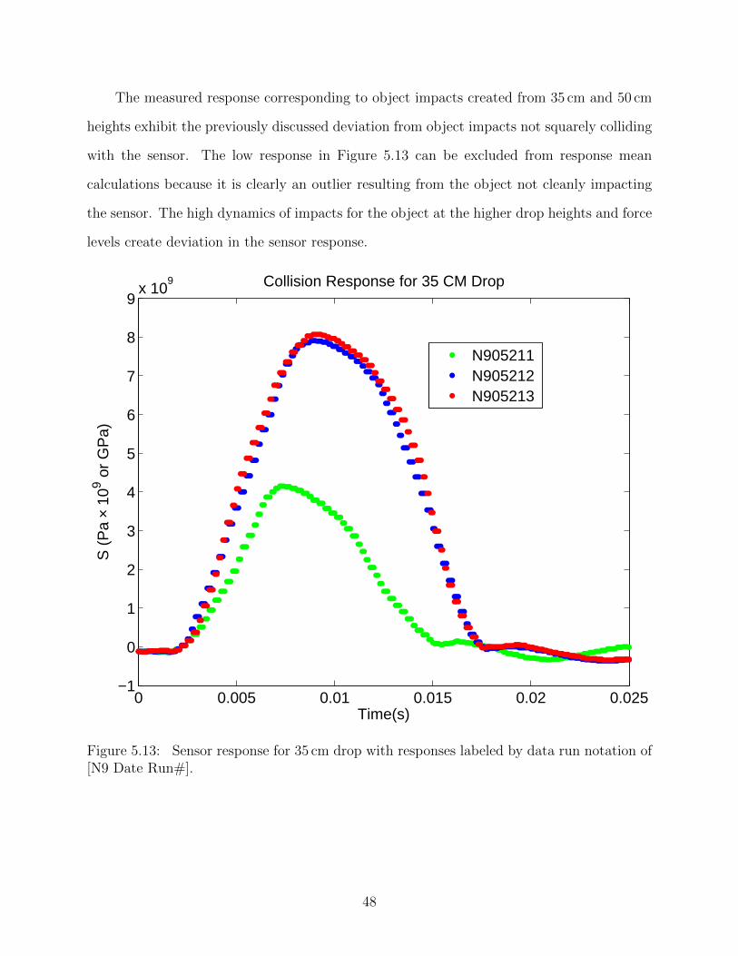
The measured response corresponding to object impacts created from 35 cm and 50 cm
heights exhibit the previously discussed deviation from object impacts not squarely colliding
with the sensor. The low response in Figure 5.13 can be excluded from response mean
calculations because it is clearly an outlier resulting from the object not cleanly impacting
the sensor. The high dynamics of impacts for the object at the higher drop heights and force
levels create deviation in the sensor response.
0 0.005 0.01 0.015 0.02 0.025−1
0
1
2
3
4
5
6
7
8
9x 10
9
S (
Pa
× 10
9 or
GP
a)
Time(s)
Collision Response for 35 CM Drop
N905211N905212N905213
Figure 5.13: Sensor response for 35 cm drop with responses labeled by data run notation of[N9 Date Run#].
48

The responses for 50 cm drops, shown in Figure 5.14, show extreme deviation such that
an accurate mean cannot be determined. However, the measured peak force for the higher
levels of dropping does not exhibit the same amount of deviation. It is likely that variation
in impact point between the object and sensor are the root cause of deviation for similar
levels of measured force. The force measurements do not deviate because the foam substrate
generates the same amount of response both on and off of the sensing tactile.
0 0.005 0.01 0.015 0.02 0.025−1
0
1
2
3
4
5
6
7
8
9x 10
9
S (
Pa
× 10
9 or
GP
a)
Time(s)
Collision Response for 50 CM Drop
N905214N905215N905216N905217N905218
Figure 5.14: Sensor response for 50 cm drop with responses labeled by data run notation of[N9 Date Run#]. The data runs show extreme deviation because of object impacts partiallyimpacting the tactile.
49

The measured sensor response for the range of collision detections, shown in Figure
5.15, shows the strong correlation of some sensor response levels while others exhibit more
deviation. Unlike the average force experimentation method where large numbers of collisions
were created (more than 30) for each level, the complexity of camera based displacement
measurement and processing limited the number of achievable collisions. The low number
of data points causes problems for sensor response measurement when the object does not
squarely strike the sensor, as previously discussed.
0 50 100 150 200 250 300 350 400 4502
3
4
5
6
7
8
9x 10
9
S (
Pa
× 10
9 or
GP
a)
Peak Impact Force (N)
Peak Collision Responses vs Peak Force
5cm10cm15cm20cm35cm50cmMean
Figure 5.15: Sensor response vs measured impact force for total data run including meanvalue line.
50
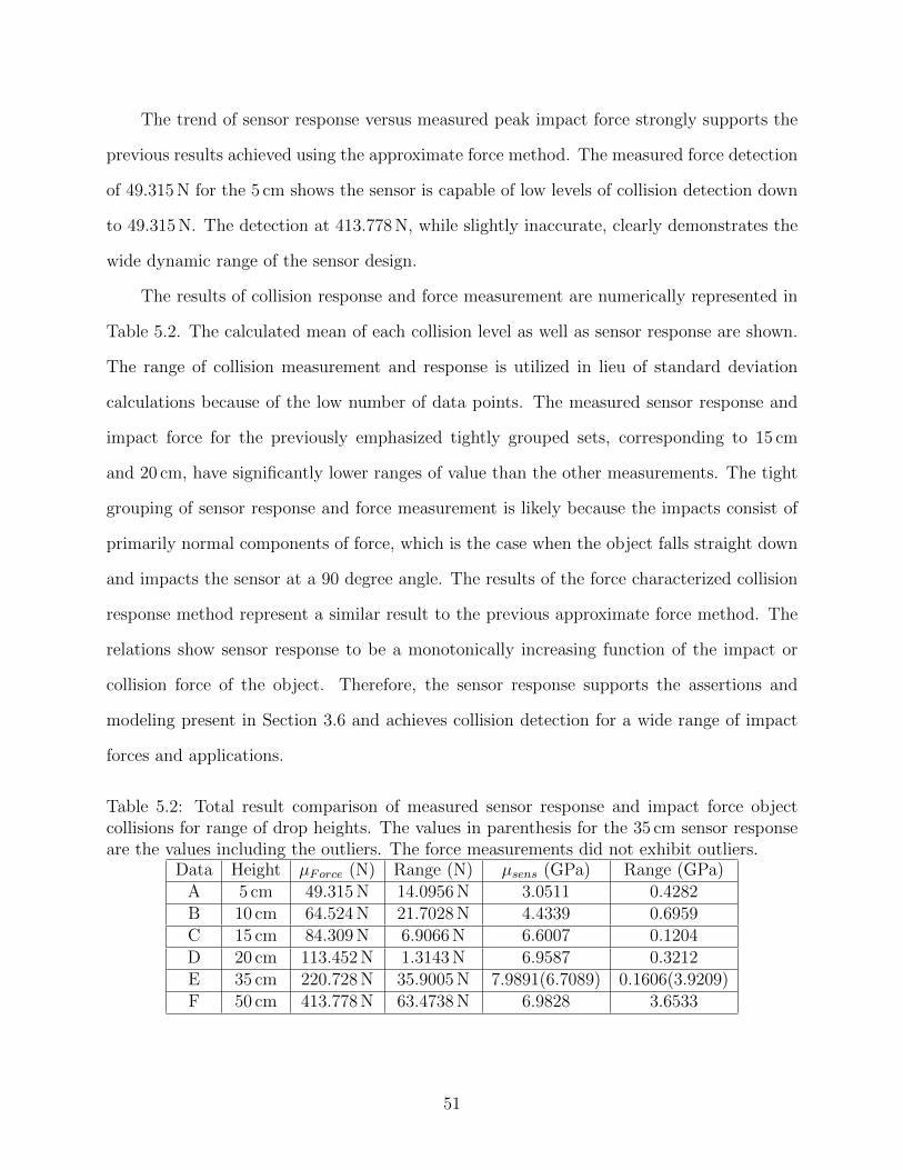
The trend of sensor response versus measured peak impact force strongly supports the
previous results achieved using the approximate force method. The measured force detection
of 49.315 N for the 5 cm shows the sensor is capable of low levels of collision detection down
to 49.315 N. The detection at 413.778 N, while slightly inaccurate, clearly demonstrates the
wide dynamic range of the sensor design.
The results of collision response and force measurement are numerically represented in
Table 5.2. The calculated mean of each collision level as well as sensor response are shown.
The range of collision measurement and response is utilized in lieu of standard deviation
calculations because of the low number of data points. The measured sensor response and
impact force for the previously emphasized tightly grouped sets, corresponding to 15 cm
and 20 cm, have significantly lower ranges of value than the other measurements. The tight
grouping of sensor response and force measurement is likely because the impacts consist of
primarily normal components of force, which is the case when the object falls straight down
and impacts the sensor at a 90 degree angle. The results of the force characterized collision
response method represent a similar result to the previous approximate force method. The
relations show sensor response to be a monotonically increasing function of the impact or
collision force of the object. Therefore, the sensor response supports the assertions and
modeling present in Section 3.6 and achieves collision detection for a wide range of impact
forces and applications.
Table 5.2: Total result comparison of measured sensor response and impact force objectcollisions for range of drop heights. The values in parenthesis for the 35 cm sensor responseare the values including the outliers. The force measurements did not exhibit outliers.
Data Height µForce (N) Range (N) µsens (GPa) Range (GPa)A 5 cm 49.315 N 14.0956 N 3.0511 0.4282B 10 cm 64.524 N 21.7028 N 4.4339 0.6959C 15 cm 84.309 N 6.9066 N 6.6007 0.1204D 20 cm 113.452 N 1.3143 N 6.9587 0.3212E 35 cm 220.728 N 35.9005 N 7.9891(6.7089) 0.1606(3.9209)F 50 cm 413.778 N 63.4738 N 6.9828 3.6533
51

Chapter 6
Conclusion
In contrast to existing technologies, the detailed sensor design developed in this the-
sis shows strong collision sensation for both planar and non-planar surfaces. The pseudo-
membrane construction eliminates not only mechanical issues associated with pressure and
membrane based sensation but also increases applicability of the PVDF sensing technology.
Furthermore, the uniform and consistent response of planar and non-planar applications
eliminates hardware specialization needs such that modular collision detection systems can
be created. The interface electronics and sensor construction is accomplished with commer-
cially producible parts such that retrofitting is easily accomplished. The results support the
theoretical relation of compressive stress to measured response in the local frame and the
sensor measurements provide a monotonically increasing output as a function of the applied
collision force. The novel sensor design in this thesis shows strong promise for a robustly
applicable collision detection solution for complex robotic arms and non-standard operating
environments.
6.1 Results Summary
The approximate force testing method utilized for characterizing the sensor show the
wide dynamic sensing range of the sensor from levels as low 5 N to values as high as 300 N.
The strong correlation and consistent results show the sensing to be capable of detecting
collision and limiting harm before significant force has occurred to the robotic system or
impact object. The force measurement supports and achieved consisten results with the
approximate method verifying the measurement. The peak force measurement cover a similar
range of 49 N to 419 N. The high level of 419 N clearly demonstrates the sensors collision
52

detection ability at high levels. The deviation of collision for object impacts which do not
squarely impact the sensor–still show a collision detection response.
6.2 Future Work
Further finite element analysis and strain modeling of the system and substrate is nec-
essary to more accurately identify the applicability of the sensor. Specifically, closed cell
foam and other elastic substrates experience stress and strain in a nonlinear manner and
more complex modeling and force measurement is required to accurately model the system.
Additionally, more extensive testing of substrate options to more accurately characterize
the effects of material properties on sensor response is needed to increase viability of con-
struction. The testing was primarily carried out using equivalent size elements and objects
to maintain continuity of the experimentation. However, additional testing using a variety
of not only different sized and shaped elements but also different sized and shaped objects
would be beneficial. The collisions utilized for testing were limited to impact collision gener-
ated from falling objects. Recall from the previously described hazard origins for mechanical
danger, different types of collisions including pinching scenarios, impact and hold scenarios–a
collision in which object is already in contact with the sensor and the robotic system ac-
tuates towards the object– are necessary to ensure the sensor enables the system to meet
current international safety standards including ISO 10218 [22, 23] and IEC 60601-1 [28].
Additional algorithm development for advanced or adaptive collision detection utilizing the
sampled signal would also benefit the work. In order to satisfy the previously mentioned
standards, routines for online calibration and sensor fault testing are necessary.
53

Bibliography
[1] A. Mirbagheri, J. Dargahi, F. Aghili, and K. Parsa, “Finite element analysis of amembrane-type piezoelectric tactile sensor with four sensing elements,” in 2005 IEEESensors, Nov. 2005, pp. 4 pp.–.
[2] L. Seminara, L. Pinna, M. Valle, L. Basirico, A. Loi, P. Cosseddu, A. Bonfiglio, A. Ascia,M. Biso, A. Ansaldo, D. Ricci, and G. Metta, “Piezoelectric polymer transducer arraysfor flexible tactile sensors,” in 2012 IEEE Sensors, Oct. 2012, pp. 1–4.
[3] S. Haddadin, A. Albu-Schaffer, A. De Luca, and G. Hirzinger, “Collision detectionand reaction: A contribution to safe physical human-robot interaction,” in IEEE/RSJInternational Conference on Intelligent Robots and Systems, IROS 2008, 2008, pp. 3356–3363.
[4] R. Schulze, T. Gessner, M. Schueller, R. Forke, D. Billep, M. Heinrich, M. Sborikas,and M. Wegener, “Integration of piezoelectric polymer transducers into microsystemsfor sensing applications,” in Applications of Ferroelectrics held jointly with 2012 Eu-ropean Conference on the Applications of Polar Dielectrics and 2012 InternationalSymp Piezoresponse Force Microscopy and Nanoscale Phenomena in Polar Materials(ISAF/ECAPD/PFM), 2012 Intl Symp, 2012, pp. 1–4.
[5] A. Yamamoto, S. Nagasawa, H. Yamamoto, and T. Higuchi, “Electrostatic tactile dis-play with thin film slider and its application to tactile telepresentation systems,” IEEETransactions on Visualization and Computer Graphics, vol. 12, no. 2, pp. 168–177, 2006.
[6] I. Fujimoto, Y. Yamada, T. Morizono, Y. Umetani, and T. Maeno, “Development ofartificial finger skin to detect incipient slip for realization of static friction sensation,” inProceedings of IEEE International Conference on Multisensor Fusion and Integrationfor Intelligent Systems, MFI2003., Jul. 2003, pp. 15–20.
[7] E. S. Kolesar and C. S. Dyson, “Object imaging with a piezoelectric robotic tactilesensor,” Journal of Microelectromechanical Systems, vol. 4, no. 2, pp. 87–96, Jun. 1995.
[8] J. M. Wooten, D. M. Bevly, and J. Y. Hung, “Robust large-area piezoelectric polymerbased collision detection sensor,” in 39th Annual Conference of the IEEE IndustrialElectronics Society (IECON-2013), Vienna, Austria,, Nov. 2013, pp. 1–6.
[9] C. S. Brown, R. C. Kell, R. Taylor, and L. A. Thomas, “Piezoelectric materials, a reviewof progress,” IRE Transactions on Component Parts, vol. 9, no. 4, pp. 193–211, 1962.
54

[10] E. Fukada, “Piezoelectricity of wood,” Journal of the Physical Society of Japan, vol. 10,no. 2, pp. 149–154, 1955. [Online]. Available: http://jpsj.ipap.jp/link?JPSJ/10/149/
[11] D. Damjanovic, “Ferroelectric, dielectric and piezoelectric properties of ferroelectric thinfilms and ceramics,” Reports on Progress in Physics, vol. 61, no. 9, p. 1267, 1998.
[12] E. Fukada, “History and recent progress in piezoelectric polymers,” IEEE Transactionson Ultrasonics, Ferroelectrics and Frequency Control, vol. 47, no. 6, pp. 1277–1290, Nov.2000.
[13] H. Kawai, “The piezoelectricity of poly (vinylidene fluoride),” Japanese Journalof Applied Physics, vol. 8, no. 7, pp. 975–976, 1969. [Online]. Available:http://jjap.jsap.jp/link?JJAP/8/975/
[14] J. Cai, X. Fu, and H. Liu, “Design of PVdf stress sensor and its application in the stresstest of foam plastic,” in 2012 International Conference on Measurement, Informationand Control (MIC), vol. 2, 2012, pp. 821–824.
[15] Y. Shapiro, A. Wolf, and G. Kosa, “Piezoelectric deflection sensor for a bi-bellowsactuator,” IEEE/ASME Transactions on Mechatronics, vol. 18, no. 3, pp. 1226–1230,2013.
[16] J. Kymissis, C. Kendall, J. Paradiso, and N. Gershenfeld, “Parasitic power harvesting inshoes,” in Second International Symposium on Wearable Computers. Digest of Papers,1998, pp. 132–139.
[17] H. Han, Y. Nakagawa, Y. Takai, K. Kikuchi, and S. Tsuchitani, “PVdf film microfabrication for the robotics skin sensor having flexibility and high sensitivity,” in 2011Fifth International Conference on Sensing Technology (ICST), 2011, pp. 603–606.
[18] T. Sekitani, T. Yokota, and T. Someya, “Ultra-flexible, ultra-thin, ultra-sensitive or-ganic pressure sensor system for biomedical applications,” in 2012 IEEE Sensors, 2012,pp. 1–3.
[19] J. Xia, Z. Xie, H. Fang, T. Lan, J. Huang, and H. Liu, “Collision detection of flexiblejoint manipulator by using joint torque sensors,” in Advanced Intelligent Mechatronics,2009. AIM 2009. IEEE/ASME International Conference on, 2009, pp. 1816–1821.
[20] H.-W. Je, J.-Y. Baek, and M.-C. Lee, “A study of the collision detection of robotmanipulator without torque sensor,” in ICCAS-SICE, 2009, 2009, pp. 4468–4471.
[21] L. Seminara, M. Capurro, P. Cirillo, G. Cannata, and M. Valle, “Electromechanicalcharacterization of piezoelectric PVdf polymer films for tactile sensors in robotics ap-plications,” Sensors and Actuators A: Physical, vol. 169, no. 1, pp. 49–58, 2011.
[22] Robots and robotic devices - Safety requirements for industrial robots: Part 1: Robots,International Standard Organization Std. ISO 10 218-1, Rev. E, 2011.
55

[23] Robots and robotic devices - Safety requirements for industrial robots: Part 2: Robotsystems and integration, International Standard Organization Std. ISO 10 218-2, Rev. E,2011.
[24] Y. Roh, V. Varadan, and V. K. Varadan, “Characterization of all the elastic, dielectric,and piezoelectric constants of uniaxially oriented poled PVdf films,” IEEE Transactionson Ultrasonics, Ferroelectrics and Frequency Control, vol. 49, no. 6, pp. 836–847, 2002.
[25] J. Gere, Mechanics of Materials, 5th ed. Brooks/Cole, 2001.
[26] F. De Lim, L. B. Tan, C. Quan, and T. Y. Tee, “Whole-field board strain and displace-ment characterization during drop impact using a single camera dic technique,” in 200911th Electronics Packaging Technology Conference. EPTC ’09., 2009, pp. 652–655.
[27] J. A. Bryson, “Impact response of polyurethane,” Ph.D. dissertation, Washington StateUniversity, December 2009.
[28] Medical electrical equipment - Part 1: General requirements for basic safety and essentialperformance, International Electrotechnical Commission Std. IEC 60 601-1, Rev. 3.1,December 2012.
[29] J. Reddy, An Introduction to Continuum Mechanics. Cambridge University Press,2008.
56

Appendix A
Material Properties
A.1 Cauchy Stress Tensor
It is important to consider the stress that exists within an object as a state of stress.
Furthermore, stress exists as combination of normal and shear stress components which
combine to form a tensor. [25]
σ =
T e1
T e2
T e3
=
σ11 σ12 σ13
σ21 σ22 σ23
σ31 σ32 σ33
=
σxx σxy σxz
σyx σyy σyz
σzx σzy σzz
=
σx τxy τxz
τyx σy τyz
τxz τyz σz
(A.1)
The Cauchy Stress Tensor is one such state of stress representation often used in contin-
uum mechanics. In this case, the stress tensor represents the components of stress for an
infinitesimally small point in the material and is defined as the current force per unit de-
formed area, σij. The stress at a point in a three-dimensional continuum can be shown using
nine quantities, three per plane, on three mutually perpendicular planes of the point.[29] The
stress components for each plane, x,y and z, are combined in Cartesian component form to
produce the second-order tensor (A.1).[29] The individual stress vectors, T ei, represent the
orthogonal components of stress for each plane. The tensor is utilized to represent complex
kinematics and statics in material which exists as a continuous combination of many small
infinitesimally small points. The Cauchy Stress tensor is unique because the symmetric
properties of the tensor allow for a stress representation of the point using only 6 elements
known as a Voigt notation; specifically, σx, σy, σz represent the normal stresses and the shear
stresses are represented by σxy, σxz, σyz, or equivalently τxy, τxz, or τyz. The symmetry of
57

the stress tensor refers to the property: σij = σji where i and j represent x, y, or z. This
symmetry is particularly useful in the strain modeling to relate experienced stress of the film
on the surface of the material to stress components of the continuous material.
A.2 Engineering Strain Tensor
ε =
ε11 ε12 ε13
ε21 ε22 ε23
ε31 ε32 ε33
=
εxx εxy εxz
εyx εyy εyz
εzx εzy εzz
=
εx
γxy2
γxz2
γyx2
εyγyz2
γxz2
γzy2
εz
(A.2)
Strain components of a material use similar notation to stress and results in a strain tensor.
The tensor includes the normal and shear strains. By considering the displacements as
small, we can neglect nonlinear terms and the resulting tensor known as the infinitesimal
strain tensor is a symmetric second-order tensor in rectangular Cartesian components. The
diagonal components of the tensor ε11,ε22, and ε23 represent the normal strains and the off
diagonal terms ε12,ε13, and ε23 represent the shear strains. The shear strains are called the
engineering shear strains and the tensor becomes the engineering strain tensor in the final
notation [29].
A.3 Geometric Representation of Strain
εij =1
2(δijo
+δjio
) (A.3)
An important material property for modeling the sensor, the geometric representation of
strain relates the normal strain to the change of length to the previous length of the material.
The combination of change in length in i and j direction represented by δi and δj respectively
divided by the original length jo and io yields the normal strain when divided by 2, εij.[25]
The geometric property is particularly useful when combined with a symmetric strain tensor
58

because measured surface strains of the film can be transformed to the normal strain of the
material.
A.4 Young’s Modulus
E =σ
ε(A.4)
The modulus of elasticity introduced by English scientist Thomas Young, Young’s Modulus,
relates the tension and compression of a material. Specifically, the Young’s Modulus of a
material is the relation of axial stress to axial strain. The modulus of elasticity is a constant
representing the slope of the stress-strain diagram in the linearly elastic region of the graph
[25]. The modulus is often used in a form known as Hooke’s law which more clearly relates
the stress of the material due to strain, shown in equation (A.5).
σ = Eε (A.5)
The typical units for E are pascals because strain, ε, is a unit less measurement and the SI
unit for stress, σ, is pascals or gigapascals.
A.5 Shear Modulus of Elasticity
G =γ
τ(A.6)
The shear modulus of elasticity is a similar relation to previously discussed Young’s Modulus.
The modulus represents the slope of the linear region of the shear stress-strain curve and is
frequently found in the Hooke’s law in shear, shown in Equation (A.7).
τ = Gγ (A.7)
59

The shear modulus of elasticity is typically expressed in pascals such that the shear stress,
τ , is in the SI unit for stress when the modulus, G, is multiplied times the unit less shear
strain, γ [25].
60


