
York University Working Paper Series
High-Order Consumption Moments and Asset Pricing
Andrei Semenov
Working Paper 2003-12-1
York University, 4700 Keele StreetToronto, Ontario M3J 1P3, Canada
April 2004
I thank Ravi Bansal, Robin Brooks, Rui Castro, George M. Constantinides, Rene Garcia,Kris Jacobs, and Eric Renault for their comments and suggestions. I also benefitted fromdiscussions with the participants in workshops and conferences at the University of Mon-treal, Ryerson and York Universities, and the 2004 Winter Meeting of the EconometricSociety in San Diego, CA.
c°2004 by Andrei Semenov. All rights reserved. Short sections of text, not to exceed twoparagraphs, may be quoted without explicit permission provided that full credit, includingc° notice, is given to the source.

Abstract
This paper investigates the role of the hypothesis of incomplete consumption insurance
in explaining the equity premium and the return on the risk-free asset. Using a Taylor
series expansion of the individual’s marginal utility of consumption around the conditional
expectation of consumption, we derive an approximate equilibrium model for expected
returns. In this model, the priced risk factors are the cross-moments of return with the
moments of the cross-sectional distribution of individual consumption and the signs of
the risk factor coefficients are driven by preference assumptions. We demonstrate that
if consumers exhibit decreasing and convex absolute prudence, then the cross-sectional
mean and skewness of individual consumption yield a larger equity premium if their cross-
moments with the excess market portfolio return are positive, while the cross-sectional
variance and kurtosis always reduce the equity premium explained by the model. Using the
data from the U.S. Consumer Expenditure Survey (CEX), we find that, in contrast to the
complete consumption insurance model, the model with heterogeneous consumers explains
the observed equity premium and risk-free rate with economically realistic values of the
relative risk aversion (RRA) coefficient (less than 1.8) and the time discount factor when
the cross-sectional skewness of individual consumption, combined with the cross-sectional
mean and variance, is taken into account.
JEL classification: G12
Keywords: equity premium puzzle, heterogeneous consumers, incomplete consumption in-
surance, limited asset market participation, risk-free rate puzzle.
Andrei Semenov
Department of Economics, York University
Vari Hall 1028, 4700 Keele Street, Toronto
Ontario M3J 1P3, Canada
Phone: (416) 736-2100 ext.: 77025
Fax: (416) 736-5987
E-mail: [email protected]

1
1 Introduction
Numerous studies have focused on a representative-agent consumption capital asset pricing
model in which asset prices are determined by the consumption and asset allocation decisions
of a single representative investor with conventional power utility. Empirical evidence is
that this model is inconsistent with the data on consumption and asset returns in many
respects. In particular, a reasonably parameterized representative-agent model generates a
mean equity premium which is substantially lower than that observed in data. This is the
equity premium puzzle. Another anomaly with the same model is that it yields the risk-free
rate which is too high compared to the observed mean return on the risk-free asset. This is
the risk-free rate puzzle.
One plausible response to the equity premium and risk-free rate puzzles is to argue that
the poor empirical performance of the representative-agent model is due to the fact that this
model abstracts from the lack of certain types of insurance such as insurance against the
idiosyncratic shocks to the households’ income or divorce, for example.1 The potential for
the incomplete consumption insurance model to explain the equilibrium behavior of stock
and bond returns, both in terms of the level of equilibrium rates and the discrepancy between
equity and bond returns, was first suggested by Mehra and Prescott (1985). Weil (1992)
studies a two-period model in which consumers face, in addition to aggregate dividend risk,
idiosyncratic and undiversifiable labor income risk and shows that decreasing absolute risk
aversion and decreasing absolute prudence are sufficient to guarantee that the model predicts
a smaller bond return and a larger equity premium than a representative-agent model
calibrated on the basis of aggregate data solely. In the infinite horizon setting, individuals
are able to make risk-free loans to one another and borrow to buffer any short-lived jump
in their consumption. This reasoning suggests that in the infinite horizon economy, the
additional demand for savings induced by incomplete consumption insurance will generally
be smaller than that in a two-period model. Hence, incomplete consumption insurance may
have little impact on interest rates. Aiyagari and Gertler (1991), Bewley (1982), Heaton
and D. Lucas (1992, 1995, 1996), Huggett (1993), Lucas (1994), Mankiw (1986), and Telmer
(1993) confirm this intuition.2
1Complete consumption insurance implies that consumers can use financial markets to diversify awayany idiosyncratic differences in their consumption streams. It follows that under the assumption of completeconsumption insurance, aggregate consumption per capita can be used in place of individual consumptionand, hence, the pricing implications of a complete consumption insurance model are similar to those ofthe representative-consumer economy. With incomplete consumption insurance, individuals are not able toself-insure against uninsurable risks and, therefore, are heterogeneous.
2In the Bewley (1982), Lucas (1994), Mankiw (1986), and Telmer (1993) models, consumers face unin-surable income risk and borrowing or short-selling constraints, whereas Aiyagari and Gertler (1991) andHeaton and D. Lucas (1992, 1995, 1996) calibrate an economy in which consumers face uninsurable incomerisk and transaction or borrowing costs. Aiyagari and Gertler (1991) and Heaton and D. Lucas (1992, 1995,

2
Unlike earlier work which assumes that the idiosyncratic income shocks are transitory
and homoskedastic, Constantinides and Duffie (1996) model the time-series process of each
consumer’s ratio of labor income to aggregate income as nonstationary and heteroskedas-
tic. Given the joint process of arbitrage-free asset prices, dividends, and aggregate income
satisfying a certain joint restriction, Constantinides and Duffie (1996) show that in the
equilibrium of an economy with heterogeneity in the form of uninsurable, persistent, and
heteroskedastic labor income shocks, the pricing kernel is a function not only of per capita
consumption growth, but also of the cross-sectional variance of the logarithmic individual
consumption growth rate. One of the key features of the Constantinides and Duffie (1996)
model is that idiosyncratic shocks to labor income must be persistent. However, using the
data from the Panel Study of Income Dynamics (PSID) Heaton and D. Lucas (1996) and
Storesletten, Telmer, and Yaron (1997) show that the conclusion whether labor income
shocks are persistent or not depends on auxiliary modelling assumptions. Brav, Constan-
tinides, and Geczy (2002) test empirically the Constantinides and Duffie (1996) pricing
kernel using the CEX database and find that this stochastic discount factor (SDF) fails to
explain the equity premium.
Balduzzi and Yao (2000) derive a SDF which differs from the Constantinides and Duffie
(1996) pricing kernel in that the second pricing factor is the difference of the cross-sectional
variance of log consumption and not the cross-sectional variance of the log consumption
growth rate. Although this SDF specification allows to explain the equity premium with
a value of the RRA coefficient which is substantially lower than that obtained using the
conventional representative-agent model, the value of risk aversion needed to explain the
equity premium remains rather high (larger than 9).
Cogley (2002) uses a Taylor series expansion of the individual’s intertemporal marginal
rate of substitution (IMRS) and develops an equilibrium factor model in which the pricing
factors for the equity premium are the cross-moments of the excess market portfolio return
with the first three moments of the cross-sectional distribution of log consumption growth.
He finds that this model is not able to explain the observed mean equity premium with
economically realistic value of risk aversion even when the model includes the first three
cross-sectional moments of log consumption growth.3
In contrast to the previous studies, Brav, Constantinides, and Geczy (2002) find em-
pirical evidence for the importance of the incomplete consumption insurance hypothesis for
explaining the equity premium. They find that the skewness of the cross-sectional distri-
1996) show that the pricing implications of an incomplete market model do not differ substantially fromthose of a representative-consumer model, unless the ratio of the net supply of bonds to aggregate incomeis restricted to an unrealistically low level.
3With low (below 5) values of the RRA coefficient, the model can explain only about one-fourth of theobserved mean equity premium.

3
bution of the individual consumption growth rate, combined with the mean and variance,
plays an important role in explaining the excess market portfolio return. Their calibration
result is that the SDF, given by a third-order Taylor series expansion of the equal-weighted
average of the household’s IMRS, reproduces the observed mean premium of the market
portfolio return over the risk-free rate with low and economically plausible (between two
and four) value of the RRA coefficient.
To investigate the role of the hypothesis of incomplete consumption insurance in explain-
ing the equity premium and the risk-free rate of return, we use a Taylor series expansion
of the individual’s marginal utility of consumption around the conditional expectation of
consumption and derive an approximate equilibrium model for expected returns.4 In this
model, the priced risk factors are the cross-moments of return with the moments of the
cross-sectional distribution of individual consumption and the signs of the risk factor coeffi-
cients are driven by preference assumptions. The attractiveness of this approach comes from
the possibility of avoiding an ad hoc specification of preferences and considering a general
class of utility functions when addressing the question of the sign of the effect of a partic-
ular moment of the cross-sectional distribution of individual consumption on the expected
excess market portfolio return and risk-free interest rate, while an ad hoc specification of
the utility function is necessary when taking a Taylor series expansion of the agent’s IMRS
or the mean of the individual’s IMRS.5 We show that if the agent’s preferences exhibit
decreasing and convex absolute prudence, then the cross-sectional mean and skewness of
individual consumption help to explain the equity premium if their cross-moments with the
excess market portfolio return are positive, while the cross-sectional variance and kurtosis
always reduce the equity premium explained by the model.
Using the data from the CEX, in our empirical investigation we apply several approaches
to assess the plausibility of the approximate equilibrium model for reproducing different
features of expected returns. First, we perform a Hansen-Jagannathan (1991) volatility
bound analysis. In this part, we assess the plausibility of the SDF for the market premium
by studying the mean and standard deviation of the pricing kernel for different values of
the risk aversion coefficient. The purpose of the calibration exercise is to test whether
the observed mean equity premium and risk-free rate can be explained with economically
plausible values of the preference parameters. Finally, we investigate the conditional version
of the Euler equations for the equity premium and the risk-free rate using a non-linear
4Mankiw (1986) and Dittmar (2002) take a Taylor series expansion of the individual’s marginal utility ofconsumption around the unconditional expectation of consumption.
5All we need to know to answer the question whether considering a particular moment of the cross-sectional distribution of individual consumption generates a smaller or, on the contrary, larger predictedasset return, is the sign of its cross-moment with return and the sign of the corresponding derivative of theutility function. Considering some special form of preferences is, however, necessary when assessing the sizeof that effect.

4
generalized method of moments (GMM) estimation approach. Here, we exploit information
about time-series properties of consumption and asset returns. In each of the three parts, the
empirical analysis is performed under the assumption of limited asset market participation.
Like Brav, Constantinides, and Geczy (2002), we find an important role played by the
hypothesis of incomplete consumption insurance in explaining asset returns. Our result is
that, in contrast to the complete consumption insurance model, both the equity premium
and the risk-free rate may be explained with economically realistic values of the RRA
coefficient (less than 1.8) and the time discount factor when the cross-sectional skewness
of individual consumption, combined with the cross-sectional mean and variance, is taken
into account. This result is robust to the threshold value in the definition of assetholders
and the estimation procedure.
The rest of the paper proceeds as follows. In Section 2, we derive an approximate
equilibrium model for the expected equity premium and risk-free rate using a general class
of utility functions. Section 3 describes the data and presents the empirical results under
the CRRA preferences. Section 4 concludes.
2 An Approximate Equilibrium Asset Pricing Model
Consider an economy in which an agent maximizes expected lifetime discounted utility:
Et
∞Xj=0
δju (Ck,t+j)
. (1)
In (1), δ is the time discount factor, Ck,t is the individual k’s consumption in period
t, u (·) is a single-period von Neumann-Morgenstern utility function, and Et [·] denotes anexpectation which is conditional on the period-t information set, Ωt, that is common to all
agents.6
Let us consider a set of agents, k = 1, ...,K, that participate in asset markets. In
equilibrium, the investor k’s optimal consumption profile must satisfy the following first-
order condition:
δEt£u0 (Ck,t+1)Ri,t+1
¤= u0 (Ck,t) , k = 1, ...,K, i = 1, ..., I. (2)
The right-hand side of (2) is the marginal utility cost of decreasing consumption by
dCk,t in period t. The left-hand side is the increase in expected utility in period t+1 which
results from investing dCk,t in asset i in period t and consuming the proceeds in period
t+ 1. Ri,t+1 is the simple gross return on asset i and I is the number of traded securities.
6We assume u (·) to be increasing, strictly concave, and differentiable.

5
For the excess return on asset i over some reference asset j, equation (2) can be rewritten
as
Et£u0 (Ck,t+1) (Ri,t+1 −Rj,t+1)
¤= 0, k = 1, ...,K, i = 1, ..., I. (3)
Assume that u (·) is N +1 times differentiable and take an N -order Taylor series expan-sion of the individual k’s marginal utility around the conditional expectation of consump-
tion, ht+1 = Et [Ck,t+1], which is assumed to be the same for all investors:
u0 (Ck,t) =NXn=0
1
n!u(n+1) (ht) (Ck,t − ht)n , k = 1, ...,K.7 (4)
Substituting (4) into (2) yields
δNXn=0
1
n!u(n+1) (ht+1) ·Et [(Ck,t+1 − ht+1)nRi,t+1] =
NXn=0
1
n!u(n+1) (ht) (Ck,t − ht)n , (5)
k = 1, ...,K, i = 1, ..., I.
We can rearrange (5) to explicitly determine expected asset returns:
Et [Ri,t+1] = δ−1NXn=0
1
n!
u(n+1) (ht)
u0 (ht+1)(Ck,t − ht)n
−NXn=1
1
n!
u(n+1) (ht+1)
u0 (ht+1)·Et [(Ck,t+1 − ht+1)nRi,t+1] , (6)
k = 1, ...,K, i = 1, ..., I.
These equations can now be summed over investors and then divided by the number of
investors in the economy to yield the following approximate relationship between expected
asset returns and priced risk factors:
Et [Ri,t+1] = δ−1NXn=0
1
n!
u(n+1) (ht)
u0 (ht+1)Zn,t −
NXn=1
1
n!
u(n+1) (ht+1)
u0 (ht+1)·Et [Zn,t+1Ri,t+1] , (7)
i = 1, ..., I, where Zn,t =1K
PKk=1 (Ck,t − ht)n.8 This is an approximate equilibrium asset
pricing model in which the priced risk factors are the cross-moments of return with the
moments of the cross-sectional distribution of individual consumption.
7Here, and throughout the paper, u(n) (·) denotes the nth derivative of u (·). Mankiw (1986) limits hisanalysis to a second-order Taylor approximation of the agent’s marginal utility of consumption (N = 2).We can interpret ht+1 as a reference consumption level. Since ht+1 is supposed to be the same for allinvestors, we may assume that it is equal to the conditional expectation of aggregate consumption percapita, ht+1 = Et [Ct+1]. Under the assumption ht+1 = E [Ct+1|Ct, Ct−1, ...], ht+1 can be defined as anexternal habit.
8A major problem with testing equation (6) directly is the observation error in reported individualconsumption. Averaging over investors seems to mitigate the measurement error effect. However, it isquite plausible that the observation error in individual consumption makes it difficult to precisely estimatethe cross-moments of return with the high-order moments of the cross-sectional distribution of individualconsumption. An issue of the measurement error effect will be addressed in Section 2.3.

6
The multifactor pricing model (7) can be seen as an attractive alternative to the mul-
tifactor models based on the Arbitrage Pricing Theory (APT). The first attractive feature
of model (7) is that, in contrast to the APT which does not provide the identification of
the risk factors, the set of factors and the form of the pricing kernel obtain endogenously
from the first-order condition of a single investor’s intertemporal consumption and portfolio
choice problem. That allows to avoid some serious problems arising from an ad hoc speci-
fication of a factor structure.9 The APT pricing models are agnostic about the preferences
of the investors. Attractive feature of model (7) is that the signs of the risk factor coeffi-
cients are driven by preference assumptions, while they are unrestricted in the multifactor
models based on the APT. The problem with both the multifactor pricing model (7) and
the multifactor models based on the APT approach is the unknown number of risk factors.
In the case of model (7), this problem translates into deciding at which point to truncate
the Taylor series expansion. This issue is explored in Section 3.3.
As previously mentioned, the conclusion about the role of consumer heterogeneity in
explaining asset returns depends on the assumed degree of shock persistence. A virtue of
our approach is that it dos not need to make any assumption about shock persistence. That
differs our approach from those by Aiyagari and Gertler (1991), Bewley (1982), Constan-
tinides and Duffie (1996), Heaton and D. Lucas (1992, 1995, 1996), Huggett (1993), Lucas
(1994), Mankiw (1986), and Telmer (1993).
2.1 Uninsurable Background Risk and the Equity Premium
The intuition that relaxing the assumption of complete consumption insurance has the
potential for explaining the equity premium puzzle is due to recognizing the fact that in
the real world, consumers face, in addition to the risk associated with the portfolio choice,
multiple uninsurable and idiosyncratic risks such as loss of employment or divorce, for
example.10
If risks are substitutes, then the presence of an exogenous risk should reduce the demand
for any other independent risk.11 Nevertheless, the presence of one undesirable risk can
make another undesirable risk desirable. This is the case of complementarity in independent
9See Campbell, Lo, and MacKinlay (1997). First, choosing factors without regard to economic theorymay lead to overfitting the data. The second potential danger is the lack of power of tests which ignore thetheoretical restrictions implied by a structural equilibrium model.10Mankiw (1986), for instance, argues that if aggregate shocks to consumption are not dispersed equally
across all consumers, then the level of the equity premium is in part attributable to the distribution ofaggregate shocks among the population. Specifically, he takes a second-order Taylor series expansion of theagent’s marginal utility around the unconditional expectation of consumption which is assumed to be thesame for all individuals and shows that the expected excess return on the market portfolio over the returnon the risk-free asset depends on the cross-moment of the equity premium with the cross-sectional varianceof individual consumption.11See Gollier and Pratt (1996), Kimball (1993), Pratt and Zeckhauser (1987), and Samuelson (1963).
7
risks.12 Whether risks are substitutes or complements may depend on their nature. It is
possible that the effect of adding one risk to another one is mixed and it is rather a question
of which effect, substitutability or complementarity in independent risks, is dominating.
Weil (1992) demonstrates that if consumers exhibit decreasing absolute risk aversion
and decreasing absolute prudence (i.e., the absolute level of precautionary savings declines
as wealth rises), then neglecting the existence of the undiversifiable labor income risk leads
to an underprediction of the magnitude of the equity premium.13 Gollier (2001) shows
that if absolute risk aversion is decreasing and convex and/or absolute risk aversion and
absolute prudence are decreasing, the presence of the uninsurable background risk in wealth
raises the aversion of a decision maker to any other independent risk. If at least one of these
sufficient conditions is satisfied, such preferences preserve substitutability in the uninsurable
background risk in wealth and the portfolio risk and, therefore, can help in solving the equity
premium puzzle. Since decreasing and convex absolute risk aversion and decreasing absolute
prudence are widely recognized as realistic assumptions, these results are overwhelmingly
in favor of substitutability in the uninsurable background risk in wealth and the portfolio
risk. It follows that the presence of the uninsurable background risk in wealth should reduce
the agent’s optimal demand for any risky asset and, therefore, should increase the expected
equity premium.
For the excess return on the market portfolio over the risk-free rate, RPt+1 = RM,t+1−RF,t+1, equation (7) reduces to
Et [RPt+1] = −NXn=1
1
n!
u(n+1) (ht+1)
u0 (ht+1)·Et [Zn,t+1RPt+1] .14 (8)
12See Ross (1999).13If consumers’ tastes exhibit decreasing absolute risk aversion and decreasing absolute prudence, then the
nonavailability of insurance against an additional idiosyncratic and undiversifiable labor income risk makesconsumers more unwilling to bear aggregate dividend risk and the equilibrium return premium on equityrises relative to the full-insurance case.14Another way to represent this equation is to rewrite it in terms of the deviations of individual consump-
tion from per capita consumption and the cross-moments of excess return with per capita consumption.In particular, when a second-order Taylor approximation of marginal utility (N = 2) is taken, (8) can berewritten as
Et [RPt+1] = −u00 (ht+1)u0 (ht+1)
·Et [(Ct+1 − ht+1)RPt+1]− 1
2
u000 (ht+1)u0 (ht+1)
×
Et£(Ct+1 − ht+1)2RPt+1
¤− 1
2
u000 (ht+1)u0 (ht+1)
·Et"PK
k=1 (Ck,t+1 − Ct+1)2K
RPt+1
#,
where Ct+1 denotes aggregate consumption per capita. The first two terms on the right-hand side of thisequation show how relative asset yields depend on the second and third cross-moments of excess return withper capita consumption, while the third term reflects influence of consumer heterogeneity on the expectedexcess return. For a higher-order Taylor approximation, a similar equation in terms of higher-order cross-moments can be derived. See Mankiw (1986).
8
Within the complete consumption insurance framework, Ck,t+1 = Ct+1, k = 1, ...,K,
and, consequently, equation (8) reduces to that in the representative-agent setting:
Et [RPt+1] = −NXn=1
1
n!
u(n+1) (ht+1)
u0 (ht+1)·Et
£Zan,t+1RPt+1
¤, (9)
where Zan,t+1 = (Ct+1 − ht+1)n and Za1,t+1 = Z1,t+1 at all t.The cross-moments of the excess market portfolio return with the moments of the cross-
sectional distribution of individual consumption can be calculated from data on individual
consumption expenditures and the excess return on the market portfolio. It follows that
to determine which effect (substitutability or complementarity in the portfolio risk and
the background risk in wealth) is generated by each of the moments of the cross-sectional
distribution of individual consumption, it suffices to sign the first five derivatives of u (·).As is conventional in the literature, we assume that the marginal utility of consumption is
positive (u0 (·) > 0) and decreasing (u00 (·) < 0), and an agent is prudent (u000 (·) > 0).15
We now turn to the signs of the fourth and fifth derivatives of u (·). Assume that absoluteprudence, AP (·), is decreasing.16
Proposition 1 Absolute prudence is decreasing (DAP) if and only if u0000 (·) < −AP (·)u000 (·).The condition u0000 (·) < 0 is necessary for DAP.
Proof. DAP implies that
AP 0 (·) = −u0000 (·)u00 (·)− (u000 (·))2
(u00 (·))2 < 0. (10)
In order to prove that the condition u0000 (·) < 0 is necessary for DAP suppose, in contrast,that u0000 (·) > 0. When u0000 (·) > 0, u0000 (·)u00 (·) 6 0 and, therefore, AP 0 (·) > 0, what
contradicts the assumption that absolute prudence is decreasing.
Inequality (10) means that u0000 (·)u00 (·) − (u000 (·))2 > 0 is the necessary and sufficient
condition for DAP. We can rewrite this condition as
u0000 (·) < (u000 (·))2u00 (·) = −AP (·)u000 (·) . (11)
Since an agent is assumed to be prudent, the term on the right-hand side of (11) is
negative.
15Kimball (1990) defines “prudence” as a measure of the sensitivity of the optimal choice of a decisionvariable to risk (of the intensity of the precautionary saving motive in the context of the consumption-savingdecision under uncertainty). A precautionary saving motive is positive when −u0 (·) is concave (u000 (·) > 0)just as an individual is risk averse when u (·) is concave.16AP (·) = −u000(·)
u00(·) > 0. Intuitively, the willingness to save is an increasing function of the expectedmarginal utility of future wealth. Since marginal utility is decreasing in wealth, the absolute level of pre-cautionary savings must also be expected to decline as wealth rises.

9
A natural assumption is that, likewise absolute risk aversion, absolute prudence is convex
(the absolute level of precautionary savings is decreasing in wealth at a decreasing rate).
Proposition 2 Absolute prudence is convex (CAP) if and only if u00000 (·) > −2AP 0 (·) ·u000 (·) − AP (·)u0000 (·). If preferences exhibit prudence and decreasing absolute prudence,then u00000 (·) > 0 is the necessary condition for CAP.
Proof. Absolute prudence is convex if the following condition is satisfied:
AP 00 (·) = −A−BC
> 0, (12)
whereA = (u00 (·))2 (u00000 (·)u00 (·)− u000 (·)u0000 (·)), B = 2u00 (·)u000 (·) (u0000 (·)u00 (·)−(u000 (·))2),and C = (u00 (·))4.
To prove that u00000 (·) > 0 is necessary for CAP under prudence and DAP, assume thatu00000 (·) 6 0. An agent is prudent (AP (·) > 0) if and only if u000 (·) > 0. By Proposition 1,we know that the necessary condition for DAP is that u0000 (·) < 0. Then, under prudenceand DAP, A > 0. Since u0000 (·)u00 (·)− (u000 (·))2 > 0 is the necessary and sufficient conditionfor DAP, prudence and DAP also imply that B < 0. In consequence, AP 00 (·) < 0, what
contradicts the initial assumption that absolute prudence is convex.
It follows from (12) that the necessary and sufficient condition for CAP is A − B < 0.This condition can be written as follows:
u00000 >2u000 (·)
³u0000 (·)u00 (·)− (u000 (·))2
´(u00 (·))2 +
u000 (·)u0000 (·)u00 (·) (13)
or, equivalently,
u00000 > −2AP 0 (·)u000 (·)−AP (·)u0000 (·) . (14)
Under prudence and DAP, the term −2AP 0 (·)u000 (·)−AP (·)u0000 (·) is positive.17So, we obtain that under DAP and CAP, u0000 (·) < 0 (the necessary condition for DAP)
and u00000 (·) > 0 (this condition is necessary for CAP). Combined with the conditions u0 (·) >0, u00 (·) < 0, and u000 (·) > 0, it follows that the cross-sectional mean and skewness of
individual consumption help to explain the equity premium if their cross-moments with the
excess market portfolio return are positive. Since the cross-moments of the equity premium
with the cross-sectional variance and kurtosis of individual consumption are always positive,
taking them into account reduces the equity premium explained by model (8).
17If an agent exhibits prudence, then AP (·) > 0 and u000 (·) > 0. The condition u0000 (·) < 0 is necessaryfor DAP.

10
2.2 Uninsurable Background Risk and the Risk-Free Rate
According to (7), the equilibrium rate of return on the risk-free asset is
Et [RF,t+1] = δ−1NXn=0
1
n!
u(n+1) (ht)
u0 (ht+1)Zn,t −
NXn=1
1
n!
u(n+1) (ht+1)
u0 (ht+1)·Et [Zn,t+1RF,t+1] (15)
or, equivalently,
Et [RF,t+1] =
µδu0 (ht+1)u0 (ht)
¶−1+
µδ−1
u00 (ht)u0 (ht+1)
Z1,t − u00 (ht+1)u0 (ht+1)
·Et [Z1,t+1RF,t+1]
+NXn=2
1
n!
Ãδ−1
u(n+1) (ht)
u0 (ht+1)Zn,t − u
(n+1) (ht+1)
u0 (ht+1)·Et [Zn,t+1RF,t+1]
!.18 (16)
When consumption insurance is complete, the expected risk-free rate is
Et [RF,t+1] =
µδu0 (ht+1)u0 (ht)
¶−1+
µδ−1
u00 (ht)u0 (ht+1)
Za1,t −u00 (ht+1)u0 (ht+1)
·Et£Za1,t+1RF,t+1
¤¶+
NXn=2
1
n!
Ãδ−1
u(n+1) (ht)
u0 (ht+1)Zan,t −
u(n+1) (ht+1)
u0 (ht+1)·Et
£Zan,t+1RF,t+1
¤!(17)
with Za1,t = Z1,t at all t.
The expected return on the risk-free asset in equations (16) and (17) is expressed as
a sum of three terms. The first term,³δ u
0(ht+1)u0(ht)
´−1, characterizes the effect of preference
for the present. Since the agent’s utility function is concave, the investor has preferences
for smoothing his consumption over time. In order to make the agent not to smooth
his consumption, the risk-free rate must be larger than³δ u
0(ht+1)u0(ht)
´−1(the consumption
smoothing effect). This effect is reflected by the second term on the right-hand side of
equations (16) and (17). The size of the consumption smoothing effect depends on the
degree of concavity of the agent’s utility function.19 When the agent is prudent and, hence,
wants to save more in order to self-insure against uninsurable risks, the risk-free rate must
be lower than³δ u
0(ht+1)u0(ht)
´−1to sustain the equilibrium (the precautionary saving effect).
The precautionary saving effect is represented by the third term on the right-hand side of
equations (16) and (17). Since Za1,t = Z1,t at all t, the first two terms on the right-hand
side of equations (16) and (17) are the same and, therefore, taking into account consumer
heterogeneity has the potential for explaining the risk-free rate puzzle if the third term on
the right-hand side of (16) is less than that in (17).
18Likewise (8), this equation can also be rewritten in terms of the cross-moments of return with percapita consumption and the cross-moments of return with the moments of the cross-sectional distributionof individual consumption.19The more concave the agent’s utility function, the higher the risk-free rate needed to compensate the
agent for not smoothing his consumption over time.

11
2.3 Measurement Error Issue
A well documented potential problem with using household level data is the large mea-
surement error in reported individual consumption.20 The widely used solution to mitigate
the impact of measurement error consists in averaging over the level of consumption or
consumption growth. Since measurement error is not observable, the choice of the optimal
method remains somewhat arbitrary and depends on what type of measurement error is
assumed.21
We assume that the observation error in the consumption level is additive. Since indi-
vidual consumption is assumed to be misreported by some stochastic dollar amount ²k,t,
the observed consumption level is Ck,t = C∗k,t+ ²k,t, where C
∗k,t is the true level of the agent
k’s consumption in period t. We further assume that for all k at all t, ²k,t ∼ D¡0,σ2²,t
¢and
²k,t is independent of the true consumption level.
By the law of large numbers, when K −→∞, 1KPKk=1Ck,t
P−→ E [Ck,t] = EhC∗k,t
iand,
hence, averaging over the level of consumption should mitigate the additive idiosyncratic
measurement error effect. It follows that when K −→∞, Zan,t −→ Za∗n,t for all n at all t andZ1,t −→ Z∗1,t at all t.22
It may be shown that
Z2,tP−→ E [Ck,t − ht]2 = E
£C∗k,t − ht
¤2+ σ2²,t, (18)
Z3,tP−→ E [Ck,t − ht]3 = E
£C∗k,t − ht
¤3+E [²k,t]
3 (19)
and
Z4,tP−→ E [Ck,t − ht]4 = E
£C∗k,t − ht
¤4+ 6σ2²,tE
£C∗k,t − ht
¤2+E [²k,t]
4 . (20)
Therefore, when the number of households in a sample is large, equations (9) and (17)
yield asymptotically unbiased estimates of the coefficient of risk aversion and δ. The same
is also true for equations (8) and (16) with N = 1. Under the assumption of consumer
heterogeneity, a Taylor series expansion of order higher than 1 can lead to biased estimates
of both the risk aversion parameter and the time discount factor δ. Observe that with
measurement error of the type assumed here, little may be said about the signs and mag-
nitudes of the biases in the estimates of the coefficient of risk aversion and δ.23 However,
20See Runkle (1991) and Zeldes (1989).21Additive measurement error suggests averaging over the level of consumption, while in the case of
multiplicative measurement error, averaging over consumption growth may be preferable.22The sign “*” means that a value is calculated using true levels of consumption.23In Section 3.5 below, we perform an empirical analysis of the effect of additive measurement error in
the consumption level on the estimates of the preference parameters in the context of the hypothesis ofincomplete consumption insurance.

12
as we can see from (18)-(20), it seems to be plausible that the magnitude of the bias in the
estimates of the moments of the cross-sectional distribution of individual consumption and,
therefore, the cross-moments of return with the moments of the cross-sectional distribution
of individual consumption increases as the order of a Taylor series expansion rises.
3 Empirical Results
In Section 2, we have shown that the hypothesis of incomplete consumption insurance has
the potential for explaining both the excess market portfolio return and the rate of return on
the risk-free asset. In this section, we assess the quantitative importance of the hypotheses
of incomplete consumption insurance and limited asset market participation for explaining
the equity premium and the risk-free rate.
A class of utility functions widely used in the literature is the set of utility functions
exhibiting an harmonic absolute risk aversion (HARA). HARA utility functions take the
following form:
u (Ct) = a
µb+
cCtγ
¶1−γ, (21)
where a, b, and c are constants, b+ cCtγ > 0, and a c(1−γ)γ > 0.24
There are three special cases of HARA utility functions.25 Constant relative risk aversion
(CRRA) utility functions can be obtained by selecting b = 0:
u (Ct) = a
µcCtγ
¶1−γ. (22)
In the special case when a = ( c/γ)γ−1(1−γ) , we get u (Ct) =
C1−γt1−γ , where γ is the RRA coefficient,
γ 6= 1.26If γ −→∞, we obtain constant absolute risk aversion (CARA) utility functions:
u (Ct) = −exp³−cbCt
´. (23)
With γ = −1, we get quadratic utility functions:
u (Ct) = a
µb+
cCtγ
¶2. (24)
It is easy to check that when the first five derivatives of the HARA utility function
exist, u0 (·) > 0 and u00 (·) < 0 imply u000 (·) > 0, u0000 (·) < 0, and u00000 (·) > 0. Given the
24The last inequality is necessary to insure that u0 (·) > 0.25See Golier (2001).26A logarithmic utility specification, u (Ct) = log (Ct), corresponds to the case when γ = 1.

13
results obtained in Section 2, it follows that any HARA class utility function may be used
when addressing the question of the effect of a particular cross-moment of return with the
moment of the cross-sectional distribution of individual consumption on the expected equity
premium and risk-free rate. For the equations derived in Section 2 to be scale-invariant,
we need b = 0 when using a HARA class preference specification. That corresponds to the
CRRA preferences.
Assuming the CRRA homogeneous preferences, u (Ck,t) =C1−γk,t −11−γ , k = 1, ...,K, we can
rewrite (8) and (16) as
Et [RPt+1] = −Et"Ã
NXn=1
1
n!(−1)n
Ãn−1Yl=0
(γ + l)
!Zn,t+1hnt+1
!RPt+1
#(25)
and
Et [RF,t+1] = δ−1µht+1ht
¶γÃ1 +
NXn=1
1
n!(−1)n
Ãn−1Yl=0
(γ + l)
!Zn,thnt
!
−Et"NXn=1
1
n!(−1)n
Ãn−1Yl=0
(γ + l)
!Zn,t+1hnt+1
RF,t+1
#.27 (26)
If consumption insurance is complete, then Zn,t+1 = Zan,t+1 and, hence, equations (25)
and (26) can be rewritten as
Et [RPt+1] = −Et"Ã
NXn=1
1
n!(−1)n
Ãn−1Yl=0
(γ + l)
!Zan,t+1hnt+1
!RPt+1
#(27)
and
Et [RF,t+1] = δ−1µht+1ht
¶γÃ1 +
NXn=1
1
n!(−1)n
Ãn−1Yl=0
(γ + l)
!Zan,thnt
!
−Et"NXn=1
1
n!(−1)n
Ãn−1Yl=0
(γ + l)
!Zan,t+1hnt+1
RF,t+1
#, (28)
respectively.
We first focus on the mean and standard deviation of the SDF derived in Section 2.
In this part, we perform the Hansen-Jagannathan volatility bound analysis to explore the
potential for our model to explain the market premium. The second part is a model cali-
bration. Here, we look for the values of the risk aversion coefficient γ and the time discount
factor δ which allow to fit the observed mean equity premium and risk-free rate. In the
27Under the CRRA preferences,Zn,t+1hnt+1
= 1K
PKk=1
³Ck,t+1−ht+1
ht+1
´n. If ht+1 is the reference level of
consumption, we can defineCk,t+1−ht+1
ht+1as a surplus consumption ratio, as in Campbell and Cochrane
(1999).

14
third part, we exploit the time series properties of consumption and asset returns and use a
non-linear GMM estimation approach to test the conditional Euler equations for the excess
market portfolio return and the risk-free rate.
3.1 Description of the Data
The Consumption Data. The consumption data used in our analysis are taken from
the CEX.28 Our measure of consumption is consumption of nondurables and services (NDS).
For each household, we calculate monthly consumption expenditures for all the disaggregate
consumption categories offered by the CEX. Then, we deflate obtained values in 1982-84
dollars with the CPI’s (not seasonally adjusted, urban consumers) for appropriate consump-
tion categories.29 Aggregating the household’s monthly consumption across these categories
is made according to the National Income and Product Account definitions of consumption
aggregates. In order to transform our consumption data to a per capita basis, we normalize
the consumption of each household by dividing it by the number of family members in the
household.
The Returns Data. The measure of the nominal market return is the value-weighted
return (capital gain plus dividends) on all stocks listed on the NYSE and AMEX obtained
from the Center for Research in Security Prices (CRSP) of the University of Chicago. The
real monthly market return is calculated as the nominal market return divided by the 1-
month inflation rate based on the deflator defined for NDS consumption. The nominal
monthly risk-free rate of interest is the 1-month Treasury bill return from CRSP. The real
monthly risk-free interest rate is calculated as the nominal risk-free rate divided by the
1-month inflation rate. Market premium is calculated as the difference between the real
market return and the real risk-free rate of interest.
28The CEX data available cover the period from 1979:10 to 1996:2. It is a collection of data on approx-imately 5000 households per quarter in the U.S. Each household in the sample is interviewed every threemonths over five consecutive quarters (the first interview is practice and is not included in the publisheddata set). As households complete their participation, they are dropped and new households move into thesample. Thus, each quarter about 20% of the consumer units are new. The second through fifth interviewsuse uniform questionnaires to collect demographic and family characteristics as well as data on monthlyconsumption expenditures for the previous three months made by households in the survey (demographicvariables are based upon heads of households). Various income information is collected in the second andfifth interviews as well as information on the employment of each household member. As opposed to thePSID, which offers only food consumption data on an annual basis, the CEX contains highly detailed dataon monthly consumption expenditures (food consumption is likely to be one of the most stable consumptioncomponents; furthermore, as is pointed out by Carroll (1994), 95% of the measured food consumption inthe PSID is noise due to the absence of interview training). The CEX attempts to account for an estimated70% of total household consumption expenditures. Since the CEX is designed with the purpose of collectingconsumption data, measurement error in consumption is likely to be smaller for the CEX consumption datacompared to the PSID consumption data.29The CPI series are obtained from the Bureau of Labor Statistics through CITIBASE.

15
Asset Holders. For the consumer units completing their participation in the first
through third quarters of 1986, the Bureau of Labor Statistics has changed, beginning
the first quarter of 1986, the consumer unit identification numbers so that the identification
numbers for the same household in 1985 (when this household has been interviewed for
the first time) and in 1986 (when it has completed its participation) are not the same. To
match consumer units between the 1985 and 1986 data tapes, we use household character-
istics which allow us to identify consumer units uniquely. As a result, we manage to match
47.0% of households between the 1985 and 1986 data tapes. The detailed description of the
procedure used to match consumer units is given in Appendix A.
In the fifth (final) interview, the household is asked to report end-of-period estimated
market value of all stocks, bonds, mutual funds, and other such securities (market value
of all securities) held by the consumer unit on the last day of the previous month as well
as the difference in this estimated market value compared with the value of all securities
held a year ago last month. Using these two values, we calculate asset holdings at the
beginning of a 12-month recall period. The consumer unit is considered as an assetholder if
the household’s asset holdings at the beginning of a 12-month recall period exceed a certain
threshold.
To assess the quantitative importance of limited participation of households in asset
markets, we consider four sets of households. The first set (SET1) consists of all consumer
units irrespectively of the reported market value of all securities. To take into consideration
that only a fraction of households participates in asset markets, we use three sets of house-
holds defined as assetholders: the first one (SET2) consists of consumer units whose asset
holdings are equal to or exceed $2 in 1999 dollars, the two others consist of all households
with reported total assets equal to or exceeding $10000 (SET3) and $20000 (SET4).30 Per
capita consumption of a set of households is calculated as the equal-weighted average of
normalized consumption expenditures of the households in the set. Obtained per capita
consumption is seasonally adjusted by using the X-11 seasonal adjustment program.31 We
seasonally adjust the normalized consumption of each household by using the additive ad-
justments obtained from per capita consumption.
30Over the period 1991-1996 about 18% of households, for whom the market value of all securities helda year ago last month is not missing, reported asset holdings of $1 at the beginning of a 12-month recallperiod. That occurs when the household reported owning securities without precising their value (see Vissing-Jorgensen (1998)). Following Vissing-Jorgensen (1998), we classify these households as nonassetholders.31Ferson and Harvey (1992) point out that since the X-11 program uses past and future information in the
time-averaging it performs, this type of seasonal adjustment may induce spurious correlation between theerror terms of a model and lagged values of the variables and, hence, may cause improper rejections of themodel based on tests of overidentifying restrictions. As alternatives to using the X-11 program, Brav andGeczy (1995) propose to use a simpler linear filter (Davidson and MacKinnon (1993)) or the Ferson-Harvey(1992) method of incorporating forms of seasonal habit persistence directly in the Euler equation.

16
Data Selection Criteria. We drop from the sample nonurban households, households
residing in student housing, households with incomplete income responses, and households
who do not have a fifth interview. Following Brav, Constantinides, and Geczy (2002), in
any given month we drop from the sample households that report in that month as zero
either their food consumption or their NDS consumption, or their total consumption, as
well as households with missing information on the above items. Additionally, we keep in
the sample only households whose head is between 19 and 75 years of age.
3.2 Estimation of the Conditional Expectation of Consumption
Since the conditional expectation of consumption, ht+1, is supposed to be the same for
all investors, we may assume it to be equal to the conditional expectation of aggregate
consumption per capita, ht+1 = Et [Ct+1] . Assuming, as in Campbell and Cochrane (1999),
a random walk model of consumption,
∆ct+1 = g + ηt+1, (29)
where ∆ct+1 = logCt+1Ct
and ηt+1 ∼ N¡0,σ2η
¢, we get
ht+1 = exp
Ãg +
σ2η2
!Ct. (30)
Table I presents the usual ML parameter estimates and tests of model (29).
3.3 Required Order of a Taylor Series Expansion
One approach to determine the order at which the expansion should be truncated is to
allow data to motivate the point of truncation.32 This approach consists in repeating the
estimation of the model for increasing values of N and truncating the expansion at the point
when further increasing in N does not significantly affect the estimation results. As Dittmar
(2002) points out, there are at least two difficulties with allowing data to determine the
required order of a Taylor series expansion. The first one is the possibility of overfitting the
data. Another problem is that when a high-order expansion is taken, preference theory no
longer guides in determining the signs of the priced risk factors. To avoid the last problem,
Dittmar (2002) proposes to let preference arguments determine the point of truncation. He
shows that increasing marginal utility, risk aversion, decreasing absolute risk aversion, and
decreasing absolute prudence imply the fourth derivative of utility functions to be negative.
Since preference assumptions do not guide in determining the signs of the higher-order
derivatives, Dittmar (2002) assumes that the Taylor series expansion terms of order higher
32See Bansal, Hsieh, and Viswanathan (1993).

17
than three do not matter for asset pricing and truncates a Taylor series expansion after
the cubic term.33 His point of view is that the advantage coming from signing the Taylor
series expansion terms outweighs a loss of power due to omitting the terms of order four
and higher.
In this paper, we let both preference theory and the data guide the truncation. The
restriction of decreasing absolute prudence allows us to sign the fifth derivative of utility
functions and, therefore, pursue the expansion further than it is usually done. Follow-
ing Dittmar (2002), we should truncate a Taylor series expansion after the cross-moment
of return with the cross-sectional kurtosis of individual consumption. The question here is
whether the cross-moments of return with the first four moments of the cross-sectional distri-
bution of individual consumption can be estimated precisely given the previously mentioned
potentially severe effect of measurement error on the estimates of the high-order moments
of the cross-sectional distribution of individual consumption. To answer this question, we
estimate the cross-moments E [Zn,t+1RPt+1] and Et [Zn,t+1RPt+1] for n ranging from 1 to
4 using an iterated GMM approach.34 We find that the precision of estimation decreases as
n rises so that for all the sets of households classified as assetholders, the null hypotheses
E [Zn,t+1RPt+1] = 0 and Et [Zn,t+1RPt+1] = 0 are not rejected statistically at the 5% level
for n = 4. This result confirms the conjecture that the observation error in reported indi-
vidual consumption can make it difficult to precisely estimate the high-order cross-sectional
moments of individual consumption and, therefore, their cross-moments with the excess
market portfolio return.
We find that the cross-moments of the equity premium with the cross-sectional variance
and skewness of individual consumption are both positive. It follows that the variance of
the cross-sectional distribution of individual consumption represents the effect of comple-
mentarity in the portfolio risk and the background risk in wealth, while the cross-sectional
skewness of individual consumption represents the effect of substitutability. Since both the
unconditional and conditional cross-moments of the equity premium with the cross-sectional
skewness of individual consumption are still estimated precisely, we limit our empirical
investigation to the first three moments of the cross-sectional distribution of individual
consumption.35
33Brav, Constantinides, and Geczy (2002) also limit their analysis to a third-order approximation whenusing a Taylor series expansion of the equal-weighted average of the household’s IMRS.34When the conditional cross-moments are estimated, the set of instruments consists of a constant and
the term inside brackets lagged one period.35Given the same problem with estimating high-order moments due to measurement error, Cogley (2002)
also stops at a third-order polynomial when taking a Taylor series expansion of the individual’s IMRS.

18
3.4 The Hansen-Jagannathan Volatility Bound Analysis
In this section, we assess the plausibility of the pricing kernel derived in Section 2 by studying
its mean and standard deviation for different values of the risk aversion coefficient.
Assuming that a candidate SDFM∗t (m) may be formed as a linear combination of asset
returns, M∗t (m) = m + (Rt −E [Rt])0 λm, Hansen and Jagannathan (1991) show that a
lower bound on the volatility of any SDF Mt, that has unconditional mean m and satisfies
the first-order condition E [MtRt] = ι, is given by
σ (M∗t (m)) =
¡(ι−mE [Rt])0Σ−1 (ι−mE [Rt])
¢1/2, (31)
where ι is the vector of ones, Rt is the vector of time-t asset gross returns, and Σ is the
unconditional variance-covariance matrix of asset returns.
When an unconditionally risk-free asset (or, more generally, an unconditional zero-
beta asset36) exists, the first-order condition for the risk-free interest rate, E [MtRF,t] = 1,
implies that the unconditional expectation of the SDF is the reciprocal of the expected
gross return on this asset, m = 1E[RF,t]
. However, the restriction of nonsingularity of the
second-moment matrix of asset returns, Σ, implies that there is no unconditionally risk-free
asset or combination of assets37 and, hence, m must be treated as an unknown parameter.
If excess returns are used, condition (31) becomes
σ (M∗t (m)) =
³m2E [Ret ]
0 eΣ−1E [Ret ]´1/2 . (32)
Here, Ret is the vector of excess returns and eΣ denotes the variance-covariance matrix ofexcess returns.38 Working with excess returns, we are allowed to assume that there is an
unconditionally risk-free asset.39 When such an asset exists, m is no longer an unknown
parameter and may be calculated from data on the risk-free interest rate.
If there is a single excess return, the lower bound on the volatility of the SDF is given
by
σ (M∗t (m)) = m
EhRei,t
iσ³Rei,t
´ . (33)
It means that the Sharpe ratio of any excess return Rei,t must obey
EhRei,t
iσ³Rei,t
´ 6 σ (M∗t (m))
m=
σ (M∗t (m))
E [M∗t (m)]
. (34)
36An asset which unconditional covariance with the SDF is zero.37At least, its identity is not known beforehand.38Rei,t = Ri,t −Rj,t is the excess return on asset i over some reference asset j.39This asset is usually used as a reference one.

19
The Hansen-Jagannathan or Sharpe ratio inequality (34) implies that for the SDF to be
consistent with a given set of asset return data, it must lie above a ray from the origin
with slope equal to the Sharpe ratio of the single risky excess return Rei,t,E[Rei,t]σ(Rei,t)
. The
only excess return used in this empirical research is the excess value-weighted return on the
market portfolio over the risk-free rate. Over the period from 1979:11 to 1996:2, the mean
market premium is 0.73% per month with a standard deviation of 4.24%. The dotted line in
Figure 1 indicates the lower volatility bound for the pricing kernels implied by the Sharpe
ratio inequality (34) and the average monthly excess return on the U.S. stock market.
Our benchmark case is the conventional representative-agent model. For this model, the
SDF in the Euler equation for the market premium is fMt+1 =³Ct+1Ct
´−γ. The black “boxes”
in Figure 1 represent mean-standard deviation pairs implied by the SDF fMt+1 for γ ranging
from 1 to 13 with increments of 1 for the set of all households in the sample (SET1). The
white “boxes” denote mean-standard deviation points for the set of households whose asset
holdings are equal to or exceed $2 (SET2). The “triangles” and the “crosses” are used for
the groups of households who reported total assets equal to or exceeding $10000 (SET3)
and $20000 (SET4), respectively.
Figure 1: Standard deviation-mean diagram. fMt+1 =³Ct+1Ct
´−γ. The dotted line indicates the
lower volatility bound for SDFs implied by the Sharpe ratio inequality (34) and the average monthly
excess return on the U.S. stock market. The solid vertical line at 1E[RF,t+1]
= 0.9979 indicates
EhfMt+1
ifor δ equal to 1. The CEX data, 1979:10 to 1996:2.
To explain a Sharpe ratio of 0.17, the conventional representative-agent model needs a

20
risk aversion coefficient γ > 10 for SET1, γ > 6 for SET2, and γ > 5 for SET3 and SET4.Although, as expected, the coefficient of risk aversion, γ, at which the mean-standard
deviation points implied by fMt+1 enter the feasible region, decreases in asset holdings, it is
only slightly different across the sets of consumer units defined as assetholders.
From
m = E [Mt+1] = E
"δ
µCt+1Ct
¶−γ#= E
hδfMt+1
i=
1
E [RF,t+1], (35)
it follows that EhfMt+1
i= 1
δE[RF,t+1]and, hence, δ = 1
E[RF,t+1]·E[fMt+1]. Given that over
the period from 1979:11 to 1996:2 the sample mean real risk-free rate is 0.21% per month,
the unconditional mean of the SDF is m = 1E[RF,t+1]
= 0.9979. The solid vertical line at
1E[RF,t+1]
= 0.9979 in Figure 1 indicates the mean of fMt+1 for δ set to 1. By looking at
Figure 1, we can see that when the mean-standard deviation points are in the admissible
region for SDFs, the mean of fMt+1 is larger than the reciprocal of the mean real risk-free
interest rate, what implies δ less than 1. However, for economically plausible (less than 3)
values of the risk aversion coefficient, fMt+1 has, in most cases, a mean which is less than1
E[RF,t+1]and, then, the Euler equation for the risk-free rate can be satisfied only with δ
larger than 1.40 This is the risk-free rate puzzle. At the same time, for the values of the
RRA coefficient in the conventional range, the SDF has a standard deviation which is much
less than that required by the Sharpe ratio. This is the equity premium puzzle.
Now, let us take a Taylor series expansion of the representative-agent’s marginal utility
of consumption around the conditional expectation of aggregate consumption per capita.
That implies the following pricing kernel:
fMt+1 = 1 +NXn=1
1
n!(−1)n
Ãn−1Yl=0
(γ + l)
!Zan,t+1hnt+1
. (36)
The Hansen-Jagannathan volatility bound analysis results for fMt+1 given by (36) for a
third-order (N = 3) Taylor series expansion of the representative-agent’s marginal utility
of consumption are presented in Figure 2. These results show that even when a third-order
Taylor series expansion is taken and only a fraction of consumers is assumed to participate in
asset markets, relatively high risk aversion is needed to make the mean-standard deviation
points enter the feasible region.
If consumption insurance is incomplete, then individuals are heterogeneous and, hence,
40For SET1, for example, the value of δ larger than 1 is required for fitting the return on the risk-freeasset for any value of γ between 2 and 7.

21
Figure 2: Standard deviation-mean diagram. fMt+1 = 1+P3n=1
1n! (−1)n
³Qn−1l=0 (γ + l)
´Zan,t+1hnt+1
.
The dotted line indicates the lower volatility bound for SDFs implied by the Sharpe ratio inequality(34) and the average monthly excess return on the U.S. stock market. The CEX data, 1979:10 to
1996:2.
the SDF in the Euler equation for the equity premium is
fMt+1 = 1 +NXn=1
1
n!(−1)n
Ãn−1Yl=0
(γ + l)
!Zn,t+1hnt+1
. (37)
The results for the SDF specification (37) corresponding to a third-order (N = 3) Taylor
series expansion of the agent’s marginal utility of consumption are shown in Figure 3.
The first mean-standard variation point above the horizontal axis corresponds to the RRA
coefficient of 0.1, successive points have relative risk aversion of 0.2, 0.3, and so on. Given
the results in Figure 3, we may conclude that taking into account consumer heterogeneity
substantially affects the mean and standard deviation of the SDF. The Hansen-Jagannathan
analysis shows that the mean-standard deviation points enter the feasible region at plausible
values of γ (less than 1), unlike the case when a representative agent within each group of
households is assumed.41 For a given value of γ, volatility of the SDF is only slightly affected
by the size of asset holdings, so that the value of risk aversion allowing to explain the market
premium does not significantly differ across sets of households.
41Although both the volatility bound and the mean-standard deviation points implied by the SDF areestimated with error, it seems, however, to be improbable that this error is so large to substantially affectthe results and to make the points enter the feasible region at implausibly high values of γ.

22
Figure 3: Standard deviation-mean diagram. fMt+1 = 1+P3n=1
1n! (−1)n
³Qn−1l=0 (γ + l)
´Zn,t+1hnt+1
.
The dotted line indicates the lower volatility bound for SDFs implied by the Sharpe ratio inequality(34) and the average monthly excess return on the U.S. stock market. The CEX data, 1979:10 to
1996:2.
3.5 Model Calibration
In this section, we address the question of whether the size of the adverse effect of the
independent background risk in wealth on the attitude towards the portfolio risk is such
that it makes it possible to explain the observed mean excess return on the market portfolio
and risk-free rate with economically realistic values of the preference parameters. The
results are presented in Table II.
As in the preceding section, our benchmark case is the conventional representative-agent
model. For this model, we calculate the unexplained mean equity premium as
v1 =1
T
T−1Xt=0
µCt+1Ct
¶−γRPt+1 (38)
for the values of the risk aversion coefficient γ increasing from 0 with increments of 0.1.42
When the RRA coefficient is set to zero, the unexplained mean premium is equal to the
sample mean of the excess market portfolio return.43 In Table II, we report the values of γ
for which the unexplained mean premium of the value-weighted market portfolio becomes
42See Brav, Constantinides, and Geczy (2002).43Over the period from 1979:11 to 1996:2, the mean premium of the value-weighted market portfolio is
0.73% per month.
23
negative. As we can see in Table II, even when limited asset market participation is taken
into consideration, the conventional representative-agent model is able to fit the observed
mean equity premium only if an individual is assumed to be implausibly risk averse.
When a Taylor series expansion of the representative-agent’s marginal utility of con-
sumption is taken, we calculate the statistic v2 as
v2 =1
T
T−1Xt=0
Ã1 +
NXn=1
1
n!(−1)n
Ãn−1Yl=0
(γ + l)
!Zan,t+1hnt+1
!RPt+1. (39)
The results in Table II show that a Taylor series expansion of any order fails to ex-
plain the mean equity premium with an economically plausible value of the RRA coef-
ficient. When a first-order Taylor series expansion is taken, the mean premium of the
value-weighted market portfolio can be explained with the RRA coefficient ranging from
22.4 to 113 for different sets of households. In the case of a third-order Taylor series ex-
pansion, the mean equity premium can be explained with the values of the RRA coefficient
which are slightly lower than those in the first-order Taylor series expansion case (between
23.2 and 63), but, nevertheless, remain too large to be recognized as economically plausible.
As the representative-agent’s marginal utility of consumption is expanded as a Taylor series
up to terms capturing the third cross-moment of the excess market portfolio return with
aggregate consumption, the statistic v2 increases as the RRA coefficient rises, so that there
is no positive value of γ allowing to fit the observed mean premium of the value-weighted
market portfolio. Under the assumption of limited asset market participation, we find some
evidence that the risk aversion coefficient decreases as the threshold value in the definition
of assetholders is raised. When the threshold value is quite large ($10000 in 1999 dollars or
larger), one can explain the mean equity premium with γ which is lower than that in the
conventional representative-agent model. However, even after limited participation is taken
into consideration, the model fails to explain the mean excess market portfolio return with
an economically realistic value of risk aversion.
Assuming incomplete consumption insurance, we calculate the unexplained mean equity
premium as
v3 =1
T
T−1Xt=0
Ã1 +
NXn=1
1
n!(−1)n
Ãn−1Yl=0
(γ + l)
!Zn,t+1hnt+1
!RPt+1. (40)
In contrast to the complete consumption insurance case, taking into account consumer
heterogeneity allows to fit the mean excess market portfolio return with an economically
plausible (between 1 and 1.8) value of the RRA coefficient when the agent’s marginal utility
of consumption is expanded as a Taylor series up to cubic terms. Under the hypothesis of
limited asset market participation, empirical evidence that the RRA coefficient decreases as

24
the threshold value rises is weak. There is no positive value of the RRA coefficient allowing
to explain the mean equity premium when the agent’s marginal utility of consumption is
expanded as a Taylor series up to terms capturing the cross-sectional variance of individual
consumption.44 Given the values of the risk aversion parameter γ which allow to explain
the observed mean premium of the value-weighted market portfolio, we estimate the time
discount factor δ needed to fit the observed mean risk-free rate as
δ =
1T
PT−1t=0
h³ht+1ht
´γ ³1 +
PNn=1
1n! (−1)n
³Qn−1l=0 (γ + l)
´Zn,thnt
´i1T
PT−1t=0
h³1 +
PNn=1
1n! (−1)n
³Qn−1l=0 (γ + l)
´Zn,t+1hnt+1
´RF,t+1
i . (41)
To test whether the obtained results are susceptible to additive measurement error in
the consumption level, we assume that observation error is normally distributed with zero
mean, ²k,t ∼ N¡0,σ2²,t
¢, and independent of true consumption. We further assume that
the cross-sectional variance of measurement error is 20% of the cross-sectional variance
of the household consumption observed in the data, σ2²,t = 0.2 1KPKk=1 (Ck,t −Ct)2. The
row “allowing for observation error” in Table II presents the results obtained when eCk,t =Ck,t+²k,t is used in the calibration. These results illustrate that in a small sample framework
with the measurement error of the type analyzed here, the estimate of γ will be biased
upward. Empirical evidence is that, in contrast to the estimate of γ, the estimate of δ is
quite sensitive to idiosyncratic observation error in the consumption level.
3.6 GMM Results
The Hansen-Jagannathan volatility bound analysis and calibration results show that the
complete consumption insurance model does not perform well. However, taking into account
asymmetry of the cross-sectional distribution of individual consumption allows to explain
both the equity premium and the return on the risk-free asset with economically realistic
values of the preference parameters. Given this result, in this section we limit our analysis
to the incomplete consumption insurance case.
An iterated GMM approach is used to test Euler equations and estimate model param-
eters. We estimate the Euler equation
Et
"Ã1 +
NXn=1
1
n!(−1)n
Ãn−1Yl=0
(γ + l)
!Zn,t+1hnt+1
!RPt+1
#= 0 (42)
44Although Brav, Constantinides, and Geczy (2002) take a Taylor series expansion of the equal-weightedsum of the household’s IMRS and not that of the agent’s marginal utility of consumption, as in our work,their results are similar to ours. Specifically, they find that when the SDF is expressed in terms of the cross-sectional mean and variance of the household consumption growth rate, the average unexplained premiumincreases as the RRA coefficient rises. When a Taylor series expansion captures the cross-sectional skewness,in addition to the mean and variance, the average unexplained excess return on the market portfolio is lessthan that for the SDF given by the equal-weighted sum of the household’s IMRS.

25
for the excess value-weighted return and the Euler equation
δEt
"Ã1 +
NXn=1
1
n!(−1)n
Ãn−1Yl=0
(γ + l)
!Zn,t+1hnt+1
!RF,t+1
#=
µht+1ht
¶γÃ1 +
NXn=1
1
n!(−1)n
Ãn−1Yl=0
(γ + l)
!Zn,thnt
!(43)
for the gross return on the real risk-free interest rate jointly exploiting three sets of instru-
ments. The first instrument set (INSTR1) consists of a constant, the real value-weighted
market return, the real risk-free rate, and the real consumption growth rate lagged one
period. The second set of instruments (INSTR2) is the first set extended with the same
variables lagged an additional period. The third set (INSTR3) has a constant, the real
value-weighted market return, the real risk-free rate, and the real consumption growth rate
lagged one, two, and three periods.
To study the role of the first three moments of the cross-sectional distribution of individ-
ual consumption in explaining the equity premium and risk-free rate puzzles, we truncate
the series expansion after the cubic term and estimate the Euler equations with N = 3. The
model is able to fit the excess return on the market portfolio and the risk-free rate with an
economically plausible (less than 1.5) and statistically significant value of risk aversion for
any set of households whatever the set of instruments (see Table III). The estimate of the
RRA coefficient is decreasing in asset holdings, as anticipated. According to Hansen’s test
of the overidentifying restrictions, the model is not rejected statistically at the 5% level.
4 Conclusions
Empirical evidence suggests that the complete consumption insurance model fails to fit
the observed equity premium with an economically plausible value of risk aversion. This
result is robust to the threshold value in the definition of assetholders and the used analysis
method.
The impact of incomplete consumption insurance on the expected equity premium is
mixed. We find that the cross-moments of the excess market portfolio return with the cross-
sectional variance and skewness of individual consumption are both positive. It follows that
the cross-sectional variance of individual consumption represents the effect of complemen-
tarity in the portfolio risk and the background risk in wealth, while the cross-sectional
skewness represents the effect of substitutability. The empirical results show that the ef-
fect of substitutability dominates. Since the used in our empirical investigation CRRA
preferences exhibit decreasing and convex absolute risk aversion and decreasing absolute
prudence, this result is in line with the results of Weil (1992) and Gollier (2001).

26
Another important result is that both the equity premium and the risk-free rate may be
explained with economically realistic values of the RRA coefficient (less than 1.8) and the
time discount factor when the cross-sectional skewness of individual consumption, combined
with the cross-sectional mean and variance, is taken into account. This result is robust to
the threshold value in the definition of assetholders and the estimation procedure.

27
APPENDIX A: Matching Consumer Units between the 1985 and1986 Data Tapes
In the CEX, each household is interviewed every three months over five consecutive quarters.
The initial interview collects demographic and family characteristics and is not placed on
the tape. Each quarter, consumer units that have completed their final interview in the
previous quarter (about one-fifth of the sample) are replaced by new households introduced
for the first time. The households remained on the tape complete their participation. For
the consumer units completing their participation in the first through third quarters of
1986, the Bureau of Labor Statistics has changed beginning the first quarter of 1986 the
consumer unit identification numbers (NEWID). As a result, the NEWIDs for the same
household in 1985 (when this household has been interviewed for the first time) and in 1986
(when it has completed its participation) are no longer the same.
To match consumer units between the 1985 and 1986 data tapes, we use the following
household characteristics:
AGE REF - age of reference person,
COMP1 - number of males age 16 and over in family,
COMP2 - number of females age 16 and over in family,
COMP3 - number of males age 2 through 15 in family,
COMP4 - number of females age 2 through 15 in family,
COMP5 - number of members under age 2 in family,
BLS URBN - area of residence (urban/rural),
BUILDING - description of building,
EDUC REF - education of reference person,
MARITAL1 - marital status of reference person,
ORIGIN1 - origin or ancestry of reference person,
POPSIZE - population size of the primary sampling unit,
REF RACE - race of reference person,
REGION - region (for urban areas only),
SEX REF - sex of reference person.
The values of the variables SEX REF, ORIGIN1, and REF RACE must be the same
for the same household on both the 1985 and 1986 data tapes. Moreover, the CEX is
constructed so that the values of the variables BLS URBN, REGION, and BUILDING are
also the same for the same consumer unit over all interviews.
As a rule, the variable POPSIZE also has the same value for the same consumer unit over
all interviews. However, on the 1985 and 1986 data tapes this variable is coded differently:

28
1985 19861 More than 4 million More than 4 million2 1.25 million - 4 million 1.20 million - 4 million3 0.385 - 1.249 million 0.33 - 1.19 million4 75 - 384.9 thousand 75 - 329.9 thousand5 Less than 75 thousand Less than 75 thousand
It follows that in the case of these two years, the same consumer unit has the same code
for POPSIZE only if in 1985 this code is 1, 2, or 5. If a consumer unit has in 1985 the code
3, then it can have in 1986 the code 2 or 3. Households having in 1985 the code 4 can have
the code 3 or 4 in 1986. It is valid for all households living in the Northeast, the Midwest,
and the South region. For consumer units residing in the West, the variable POPSIZE is
suppressed by the Bureau of Labor Statistics on the 1986 data tape.
It is more difficult to deal with the variables MARITAL1, EDUC REF, COMP1, COMP2,
COMP3, COMP4, and COMP5 which can take different values over interviews. For these
variables, we determine the set of all possible values that they can take in 1986 given their
values in 1985.
The variable MARITAL1 is coded as follows:
1 Married2 Widowed3 Divorced4 Separated5 Never married
If a reference person is married today, then tomorrow he may be either married or
widowed, or divorced, or separated. If he is widowed or divorced, he may either keep this
status or be married. In the case, when a reference person is separated, he remains to be
separated or else becomes to be widowed or divorced. A never married person can either
keep this marital status or be married.
Let COMP1h,t denote the number of males age 16 and over in family h in period t,
COMP2h,t - the number of females age 16 and over, COMP3h,t - the number of males age 2
through 15, COMP4h,t - the number of females age 2 through 15, COMP5h,t - the number
of members under age 2 in family, SUM Th,s = COMP3h,s + COMP4h,s + COMP5h,s -
the total number of children age 15 and under in family in any period s (s > t, t = 2, 3, 4),
SUM Mh,s = COMP1h,s + COMP3h,s and SUM Fh,s = COMP2h,s + COMP4h,s - the
total number of males age 2 and over and the total number of females age 2 and over,
respectively.
We apply the following restrictions:
COMP5h,t 6 SUM Th,s (A.1)

29
and
COMP3h,t 6 SUM Mh,s 6 COMP1h,t + COMP3h,t + COMP5h,t. (A.2)
It follows that
0 6 SUM Mh,s − COMP3h,t 6 COMP1h,t + COMP5h,t. (A.3)
Similarly, for SUM Fh,s we get
COMP4h,t 6 SUM Fh,s 6 COMP2h,t + COMP4h,t + COMP5h,t (A.4)
and
0 6 SUM Fh,s − COMP4h,t 6 COMP2h,t + COMP5h,t. (A.5)
Finally,
SUM Mh,s + SUM Fh,s 6 COMP1h,t +COMP2h,t + COMP3h,t (A.6)
+COMP4h,t + COMP5h,t.
In the CEX, the variable EDUC REF is coded as follows:
1 Elementary (1-8 years)2 High school (1-4 years), less than High school graduate3 High school graduate (4 years)4 College (1-4 years), less than College graduate5 College graduate (4 years)6 More than 4 years of college7 Never attended school
Changing the code from 7 to 0 enables us to introduce the restriction:
EDUC REFh,s −EDUC REFh,t 6 1. (A.7)
We apply the following restriction to the value of the variable AGE REF:
AGE REFh,t 6 AGE REFh,s. (A.8)
To match consumer units between the 1985 and 1986 data tapes, we define three groups
of households. The first group consists of consumer units that should have the following
stream of interviews: the second interview in the second quarter of 1985, the third - in the
third quarter of 1985, the fourth - in the fourth quarter of 1985, and the fifth interview
in the first quarter of 1986. For this group, we construct two data sets. In the 1985 data
set, we include all households who completed at least one of the interviews in 1985. The

30
1986 data set consists of households who completed their fifth interview in the first quarter
of 1986. As a second group are considered consumer units whose second interview should
happened in the third quarter of 1985, the third - in the fourth quarter of 1985, the fourth
- in the first quarter of 1986, and the fifth interview should happened in the second quarter
of 1986. For this group, the 1985 data set includes all consumer units who completed at
least one interview in 1985 and the 1986 data set consists of households who completed at
least one of the interviews in 1986. In the third group of households, we include consumer
units that should have the second interview in the fourth quarter of 1985, the third - in the
first quarter of 1986, the fourth - in the second quarter of 1986, and the fifth interview in
the third quarter of 1986. For this group of consumer units, the 1985 data set consists of all
households who completed their second interview in the fourth quarter of 1985 and the 1986
data set consists of consumer units who completed in 1986 at least one of the interviews.
So, for each group of consumer units there are two data sets (one for 1985 and another
one for 1986). To find the same household in both data sets, each consumer unit included
in the 1986 data set is compared with each household included in the 1985 data set for the
same group of households. As a result, for the first group of consumer units there are 521
households (in 1019 included in the 1986 data set, 51.1%), for which we find households
with appropriate characteristics in the corresponding 1985 data set. For the second group,
this number is 756 (in 1612 consumer units, 49.6%). For the third group, we match 807
households (in 1800, 44.8%). For all the three groups, the number of matched households
is 2084 (in 4431 included in the 1986 data sets, 47.0%).45
45In order to see how well this procedure works, we test it using the 1986 and 1987 data tapes (in boththese years, the same household has the same NEWID) for the first group of consumer units constructedin the same way as in the case of using the 1985 and 1986 data tapes. There are 1465 households whocompleted their fifth interview in the first quarter of 1987 and 1787 consumer units included in the 1986data set. Only 1344 in 1465 households have at least one interview happened in 1986. As a result, we match1281 households (95.3% of the real number). In 96% of the cases, there is only one household in the 1986data set corresponding to the household included in the 1987 data set. In only 4% of the cases, there aremore than 1 (between 2 and 4) corresponding households.

31
APPENDIX B: Tables
Table I
Parameter Estimates and Tests of Model ∆ct+1 = g + ηt+1
The sampling period is from 1979:10 to 1996:2. Four sets of households are considered. The first set(SET1) consists of all consumer units irrespectively of the reported market value of all securities.We use three sets of households classified as assetholders: SET2 consists of households who reportedasset holdings equal to or exceeding $2 in 1999 dollars, SET3 and SET4 consist of households whoreported total assets equal to or exceeding $10000 and $20000, respectively. The model is estimatedby ML. Standard errors in parentheses.
Parameters SET1 SET2 SET3 SET4
g 0.0016 0.0022 0.0027 0.0021
(0.0014) (0.0023) (0.0029) (0.0032)
σ2η 0.0004 0.0010 0.0016 0.0020
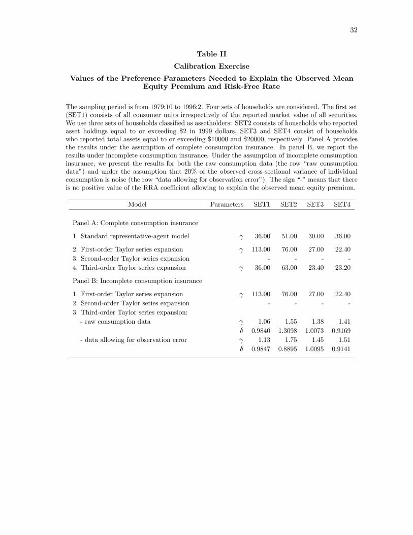
32
Table II
Calibration Exercise
Values of the Preference Parameters Needed to Explain the Observed MeanEquity Premium and Risk-Free Rate
The sampling period is from 1979:10 to 1996:2. Four sets of households are considered. The first set(SET1) consists of all consumer units irrespectively of the reported market value of all securities.We use three sets of households classified as assetholders: SET2 consists of households who reportedasset holdings equal to or exceeding $2 in 1999 dollars, SET3 and SET4 consist of householdswho reported total assets equal to or exceeding $10000 and $20000, respectively. Panel A providesthe results under the assumption of complete consumption insurance. In panel B, we report theresults under incomplete consumption insurance. Under the assumption of incomplete consumptioninsurance, we present the results for both the raw consumption data (the row “raw consumptiondata”) and under the assumption that 20% of the observed cross-sectional variance of individualconsumption is noise (the row “data allowing for observation error”). The sign “-” means that thereis no positive value of the RRA coefficient allowing to explain the observed mean equity premium.
Model Parameters SET1 SET2 SET3 SET4
Panel A: Complete consumption insurance
1. Standard representative-agent model γ 36.00 51.00 30.00 36.00
2. First-order Taylor series expansion γ 113.00 76.00 27.00 22.40
3. Second-order Taylor series expansion - - - -
4. Third-order Taylor series expansion γ 36.00 63.00 23.40 23.20
Panel B: Incomplete consumption insurance
1. First-order Taylor series expansion γ 113.00 76.00 27.00 22.40
2. Second-order Taylor series expansion - - - -
3. Third-order Taylor series expansion:
- raw consumption data γ 1.06 1.55 1.38 1.41
δ 0.9840 1.3098 1.0073 0.9169
- data allowing for observation error γ 1.13 1.75 1.45 1.51
δ 0.9847 0.8895 1.0095 0.9141

33
Table III
GMM Results under Incomplete Consumption Insurance
The sampling period is from 1979:10 to 1996:2. Four sets of households are considered. The first set(SET1) consists of all consumer units irrespectively of the reported market value of all securities.We use three sets of households classified as assetholders: SET2 consists of households who reportedasset holdings equal to or exceeding $2 in 1999 dollars, SET3 and SET4 consist of households whoreported total assets equal to or exceeding $10000 and $20000, respectively. The agent’s marginalutility of consumption is expanded as a Taylor series up to cubic terms (N = 3). The Euler equationfor the excess value-weighted market return is estimated jointly with the Euler equation for the realrisk-free interest rate using an iterated GMM approach (standard errors in parentheses). Three setsof instruments are exploited. The first instrument set (INSTR1) consists of a constant, the realvalue-weighted market return, the real risk-free rate, and the real consumption growth rate laggedone period. The second set of instruments (INSTR2) is the first set extended with the same variableslagged an additional period. The third set (INSTR3) has a constant, the real value-weighted marketreturn, the real risk-free rate, and the real consumption growth rate lagged one, two, and threeperiods. The J statistic is Hansen’s test of the overidentifying restrictions. The P value is themarginal significance level associated with the J statistic.
Parameters SET1 SET2 SET3 SET4
INSTR1
γ 1.2126 1.1282 0.0715 0.0848
(0.0505) (0.0780) (0.0189) (0.0223)
δ 0.9901 1.0113 0.9978 0.9977
(0.2349) (0.0223) (0.0005) (0.0005)
J statistic 4.9871 7.1099 7.6519 7.7094
P value 0.7590 0.5248 0.4682 0.4624
INSTR2
γ 1.1495 1.4911 1.3999 1.4609
(0.0296) (0.0574) (0.0554) (0.0584)
δ 0.9878 0.9854 1.0138 0.9733
(0.0517) (0.0971) (0.0595) (0.1049)
J statistic 6.5296 8.9943 8.2458 7.6449
P value 0.9813 0.9137 0.9412 0.9587
INSTR3
γ 1.0611 0.0128 0.0077 0.0091
(0.0206) (0.0016) (0.0014) (0.0011)
δ 0.9977 0.9988 0.9982 0.9979
(0.0231) (0.0001) (0.0001) (0.0001)
J statistic 8.9334 9.4825 9.5840 9.6172
P value 0.9977 0.9964 0.9961 0.9960

34
References
[1] Aiyagari, R.S. and M. Gertler, 1991, Asset Returns with Transactions Costs and Unin-
sured Individual Risk, Journal of Monetary Economics 27, 311-331.
[2] Balduzzi, P. and T. Yao, 2000, Does Heterogeneity Matter for Asset Pricing?, working
paper.
[3] Bansal, R., D.A. Hsieh, and S. Viswanathan, 1993, A New Approach to International
Arbitrage Pricing, Journal of Finance 48, 1719-1747.
[4] Bewley, T.F., 1982, Thoughts on Tests of the Intertemporal Asset Pricing Model,
working paper, Evanston, Ill.: Northwestern University.
[5] Brav, A., G.M. Constantinides, and C.C. Geczy, 2002, Asset Pricing with Heteroge-
neous Consumers and Limited Participation: Empirical Evidence, Journal of Political
Economy 110, 793-824.
[6] Brav, A. and C.C. Geczy, 1995, An Empirical Resurrection of the Simple Consumption
CAPM with Power Utility, working paper, University of Chicago.
[7] Campbell, J. and J. Cochrane, 1999, By Force of Habit: A Consumption-Based Expla-
nation of Aggregate Stock Market Behavior, Journal of Political Economy 107, 205-251.
[8] Campbell, J.Y., A.W. Lo, and A.C. MacKinlay, 1997, The Econometrics of Financial
Markets, Princeton University Press.
[9] Cogley, T., 2002, Idiosyncratic Risk and the Equity Premium: Evidence from the
Consumer Expenditure Survey, Journal of Monetary Economics 49, 309-334.
[10] Constantinides, G.M. and D. Duffie, 1996, Asset Pricing with Heterogeneous Con-
sumers, Journal of Political Economy 104, 219-240.
[11] Davidson, R. and J.G. MacKinnon, 1993, Estimation and Inference in Econometrics,
Oxford University Press.
[12] Dittmar, R.F., 2002, Nonlinear Pricing Kernels, Kurtosis Preference, and Evidence
from the Cross Section of Equity Returns, Journal of Finance 57, 369-403.
[13] Ferson, W.E. and C.R. Harvey, 1992, Seasonality and Consumption-Based Asset Pric-
ing, Journal of Finance 47, 511-552.
[14] Gollier, C., 2001, The Economics of Risk and Time, The MIT Press, Cambridge,
Massachusetts, London, England.

35
[15] Gollier, C. and J.W. Pratt, 1996, Risk Vulnerability and the Tempering Effect of
Background Risk, Econometrica 64, 1109-1124.
[16] Hansen, L.P. and R. Jagannathan, 1991, Implications of Security Market Data for
Models of Dynamic Economies, Journal of Political Economy 99, 225-262.
[17] Heaton, J. and D.J. Lucas, 1992, The Effects of Incomplete Insurance Markets and
Trading Costs in a Consumption-Based Asset Pricing Model, Journal of Economic
Dynamics and Control 16, 601-620.
[18] Heaton, J. and D.J. Lucas, 1995, The Importance of Investor Heterogeneity and Fi-
nancial Market Imperfections for the Behavior of Asset Prices, Carnegie-Rochester Ser.
Public Pol.
[19] Heaton, J. and D.J. Lucas, 1996, Evaluating the Effects of Incomplete Markets on Risk
Sharing and Asset Pricing, Journal of Political Economy 104, 443-487.
[20] Huggett, M., 1993, The Risk-Free Rate in Heterogeneous-Agent Incomplete-Insurance
Economies, Journal of Economic Dynamics and Control 17, 953-969.
[21] Kimball, M.S., 1990, Precautionary Savings in the Small and in the Large, Economet-
rica 58, 53-73.
[22] Kimball, M.S., 1993, Standard Risk Aversion, Econometrica 61, 589-611.
[23] Lucas, D.J., 1994, Asset Pricing with Undiversifiable Income Risk and Short Sales
Constraints: Deepening the Equity Premium Puzzle, Journal of Monetary Economics
34, 325-341.
[24] Mankiw, N.G., 1986, The Equity Premium and the Concentration of Aggregate Shocks,
Journal of Financial Economics 17, 211-219.
[25] Mehra, R. and E.C. Prescott, 1985, The Equity Premium: A Puzzle, Journal of Mon-
etary Economics 15, 145-162.
[26] Pratt, J.W. and R.J. Zeckhauser, 1987, Proper Risk Aversion, Econometrica 55, 143-
154.
[27] Ross, S.A., 1999, Adding Risks: Samuelson’s Fallacy of Large Numbers Revisited,
Journal of Financial and Quantitative Analysis 34, 323-340.
[28] Runkle, D.E., 1991, Liquidity Constraints and the Permanent-Income Hypothesis: Ev-
idence from Panel Data, Journal of Monetary Economics 27, 73-98.
36
[29] Samuelson, P.A., 1963, Risk and Uncertainty: the Fallacy of the Law of Large Numbers,
Scientia 98, 108-113.
[30] Storesletten, K., C.I. Telmer, and A. Yaron, 1997, Persistent Idiosyncratic Shocks and
Incomplete Markets, unpublished manuscript.
[31] Telmer, C.I., 1993, Asset-Pricing Puzzles and Incomplete Markets, Journal of Finance
48, 1803-1832.
[32] Vissing-Jorgensen, A., 1998, Limited Stock Market Participation, working paper.
[33] Weil, P., 1992, Equilibrium Asset Prices with Undiversifiable Labor Income Risk, Jour-
nal of Economic Dynamics and Control 16, 769-790.
[34] Zeldes, S., 1989, Consumption and Liquidity Constraints: An Empirical Investigation,
Journal of Political Economy 97, 305-346.


