Transactions, SMiRT-23
Manchester, United Kingdom - August 10-14, 2015
Division I, Paper ID 218
High temperature specific heat measurement using quasi-adiabatic calorimetry
Mark Kirkham1,, Klaus Nuemann
2, Andrew Wisbey
1, and Bryan Daniels
2
1 Amec Foster Wheeler, Clean Energy, Walton House, Birchwood Park, Warrington, Cheshire,, UK
2 Physics Department Loughborough University, UK
ABSTRACT The measurement of specific heat capacity above ambient temperatures is normally performed using
differential scanning calorimeters (DSC’s), which typically use small samples (5 mm x 1 mm, up to 5 mm
x 15 mm). However, some materials (e.g. graphite, complex alloys, polymers and composites) require a
large number of grains, or large volumes, for measurements to be representative of a material’s bulk
properties. For these types of material DSC measurements are not ideal and traditional modelling (i.e.
Kopp-Neumann, method of mixtures) has only limited applications and is not always applicable,
especially if phase changes take place, or the sample melts.
Low temperature specific heat capacity has been successfully measured using Nernst-type (heat pulse)
adiabatic calorimetry. This technique has potentially the best accuracy of available techniques and a large
freedom on sample size. Therefore, a high temperature quasi-adiabatic calorimeter was developed.
The developed system uses a quasi-adiabatic sample mounting arrangement to measure specific heat,
using an integrated temperature sensor and heater arrangement for improved sensitivity. During the
development of the measurement system two methods of heat pulse analysis were produced; 1.traditional
post-pulse regression/interpolation, and 2. a simplified finite element modelling technique The system
and both analysis techniques produced reproducible specific heat capacity data between room temperature
and 1000°C on samples sizes between 2 g to 50 g for graphite, copper, stainless steel, and molybdenum
samples. This data compared well with accepted values for these materials.
INTRODUCTION As part of a programme of research investigating the shape memory effect in the ferritic shape memory
alloy Ni2MnGa at Loughborough University Physics department a method of determining the high
temperature order-disorder phase transition (V. Recarte, 2012) (Khovailo, et al., 2001) of as cast non-
stoichimetric compositions of Ni2MnGa (Reece, 2007) using specific heat capacity was required
(Kirkham, 2014). The relatively large grain structure and potential for segregation that can occur in cast
Ni2MnGa (Cherneko, et al., 1994) meant that DSC measurements were not considered ideal, as this
technique would limit sample size and potentially skew results. To allow for a larger sample size and
potentially increase resolution at the transition temperature, a system for the measurement of specific heat
adiabatically was developed. The following sections of this paper detail the apparatus used, the analysis
techniques applied and the results of commissioning tests performed with a range of material.
METHODOLOGY The high temperature adiabatic calorimeter (referred to as the HTCP system) measures specific heat using
the Nernst-type pulsed technique (Nernst, 1911). This consists of a sample being heated/cooled to the
required measurement temperature, once stable, a known amount of energy is supplied to the sample (the
heat pulse) and the resultant change in temperature recorded. If the sample is perfectly thermally isolated
during the measurement (adiabatic) the specific heat capacity can be determined directly using the
equation below:
23rd
Conference on Structural Mechanics in Reactor Technology
Manchester, United Kingdom - August 10-14, 2015
Division I
dT
dQ
mCP
1= (1)
Where m = mass, dQ = supplied energy, and dT = change in sample temperature
In practise the sample is never perfectly thermally isolated and there is always some heat loss from the
sample and much of the design and development effort for the HTCP system focused on minimizing heat
loss and correcting for unpreventable heat loss and other practical considerations (e.g. additional thermal
mass due to heater and measurement apparatus).
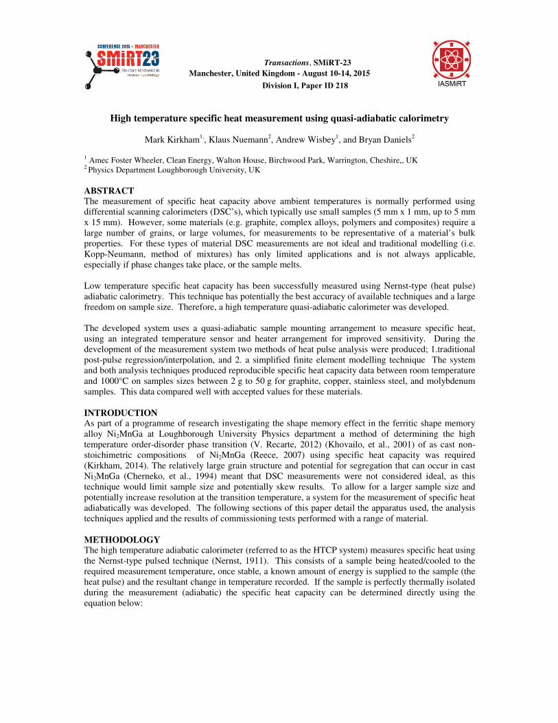
Description of Apparatus The HTCP system consists of: a furnace to heat the sample to the measurement temperature; a vacuum
tube, in which the measurement apparatus is located: a number of radiations shields and internal supports;
and the sample head, containing the sample and measurement apparatus (i.e. thermocouples, sample
heater, etc). Figure 1 shows a cross section of the test apparatus.
(a) (b)
Figure 1: Cross sections of (a) the HTCP test chamber, and (b) the sample head containing the sample and
measurement apparatus.
All measurements were performed inside the vacuum tube, evacuated to <2x10⁻³
mbar, to prevent
convective heat loss from the sample. Testing in vacuum also reduced oxidation to the samples and the
internal supports when at high temperature. The inserts supporting the sample head and radiation shields
(Figure 1a) were all made of thin walled stainless steel tube to minimise longitudinal heat transfer and
permit the sample can to remain at a stable temperature. The horizontal radiation shields/baffles along the
tube (Figure 1a) were made of thin molybdenum foil, these components minimise longitudinal heat
transfer away from the sample head due to radiation.
The sample head (Figure 1b) containing the sample and measurement apparatus was positioned at the
mid-point of the furnace hot zone (Figure 1a), where the temperature was uniform and stable. The hot
zone extended 200 mm above and below the ends of the head. The outer surface of the sample head was
made of thick ceramic (alumina and boron nitride) with molybdenum attachments. The thickness of the

23rd
Conference on Structural Mechanics in Reactor Technology
Manchester, United Kingdom - August 10-14, 2015
Division I
outer shell (4 mm alumina, and 8 mm boron nitride) was maximised to increase thermal mass and heat
transfer time to prevent any short term temperature fluctuation affecting the sample and to allow for a
more stable internal temperature.
Inside the ceramic outer shell of the sample head a number of floating molybdenum and tantalum
radiation shields were mounted concentrically around the sample to minimize radiative heat loss from the
sample during pulse measurements. To reduce conductive heat loss during pulse measurements the
sample was suspended from fine wires welded to the sample surface. To reduce the sample connections,
these support wires double as thermocouples used to measure the sample surface temperature.
A small wire wound platinum resistance thermometer (PT100) was cemented in a hole drilled in the
centre of the sample to act as a combined temperature sensor and sample heater element (See Figure 1b).
The sample heater was connected using the four-point probe configuration to permit accurate
determination of the sensor resistance and the power supplied during heating, without the resistance of the
connecting wires having an effect.
The instrumentation in the sample head (2 off K-type thermocouples and 4 off wires connected to PT100
thermometer) was connected through water cooled lead-throughs in the vacuum tube head to a
multiplexer unit, power source and measurement instrumentation. A computer connected to these
components control the system and records all measurements in real-time.
Initial Trials During initial trials two aspects of the measurement approach required further consideration. These were
the sample temperature measurements and sample temperature stability (due to thermal isolation).
Figure 2: HTCP heat pulse signal with thermocouple (red) and platinum resistance thermometer (blue)
temperature data.
Sample Temperature:
Nernst-type heat pulse calorimeters determine the change in temperature (dT) due to a heat pulse by
measuring the sample temperature after a heat pulse and subtracting a baseline temperature determined
from the pre-heat pulse stage of a measurement. Figure 2 shows a heat pulse for copper at room
temperature, as can be seen the change in sample temperature recorded by the thermocouple (red line,
Figure 2) is much lower than observed in PT100 resistor data (blue line, Figure 2). Analysis of both data
sets below shows an error of 22% on the specific heat derived from the thermocouple data but only 1.2%
for that based upon the PT100 sensor. This suggests that the surface thermocouple was insufficiently
sensitive to accurately determine the sample temperature change during a heat pulse. Hence the heater
element (PT100 resistance thermometer) was used. While the surface mounted thermocouples were of
limited application for determining the sample dT for a heat pulse, they were useful in calibrating each
PT100 sensor used.
-0.5
0
0.5
1
1.5
2
2.5
3
3.5
��� ��� ��� ��� ��� ��� ��� ��� ���
Time (s)
dT (K
)
RST offset
Sample
23rd
Conference on Structural Mechanics in Reactor Technology
Manchester, United Kingdom - August 10-14, 2015
Division I
Sample temperature stability (due to thermal isolation):
The configuration of the HTCP system, and location of the sample (Figure 1) gave excellent thermal
isolation of the sample from the furnace but the time taken for the sample to stabilise after a 10 K change
in furnace temperature was in excess of 2 hours. Under this configuration, the long delay between heat
pulse measurements (due to slow stabilising rate) would mean that a specific heat measurement between
room temperature and 1300 K (measurements made every 10 K), would take more than 16 days (for both
heating and cooling phases). This time does not include the time taken for the pulse measurements. This
is clearly impractical for most purposes and limits the observations possible.
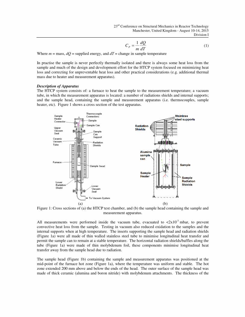
To address this problem and reduce the test time and also increase resolution it was proposed that instead
of allowing the sample to stabilise at a specific temperature before making the measurement, the furnace
and sample should be heated linearly and the pulse measurements made continuously with a suitable gap
to allow the residual heat from any heat pulse to dissipate and the sample to return a pre-heat pulse
thermal drift (Figure 3).
Figure 3: Schematic of a heat pulse made with a linearly drifting baseline.
The advantage of the linearly drifting baseline is that not only does it reduce measurement time (without
affecting resolution), but it also allows for the measurement of dynamic processes. However, this
approach does mean that there are additional potential sources of error in the measurement and the system
cannot be described as truly adiabatic.
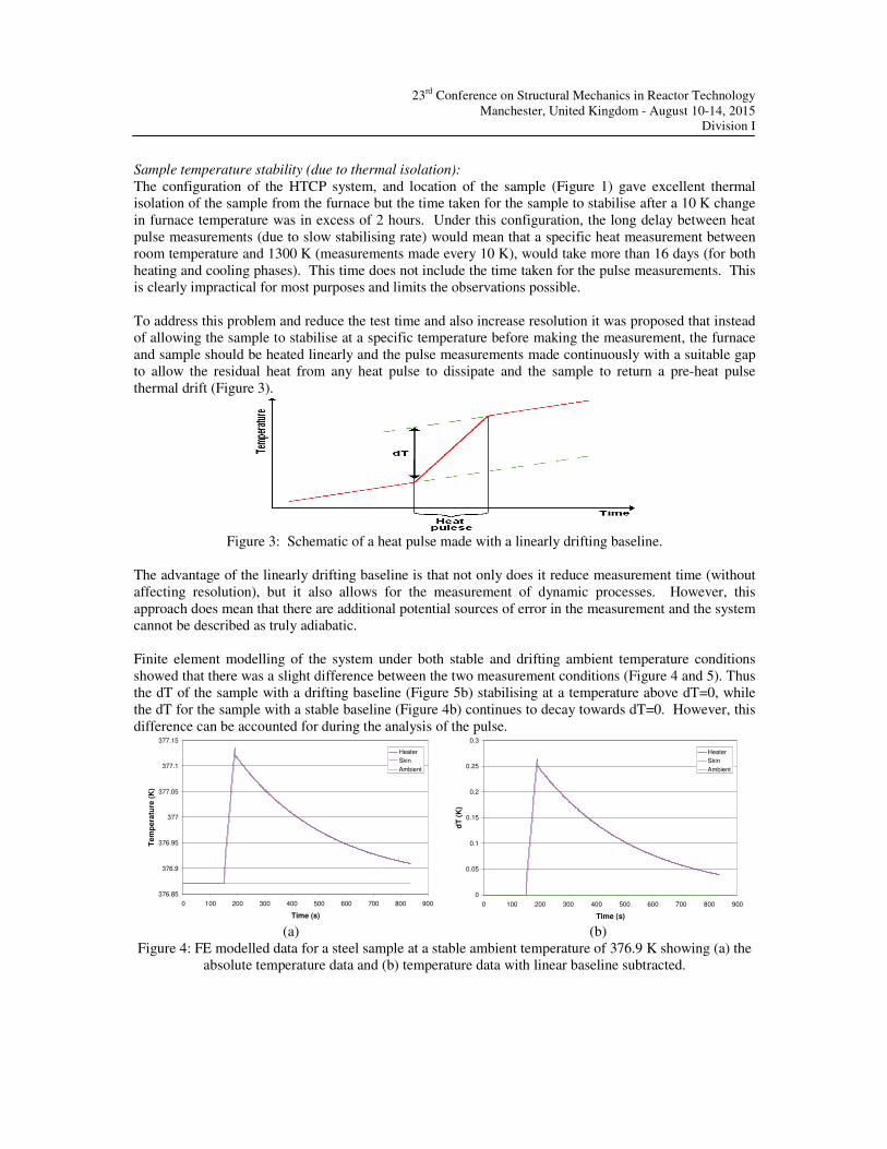
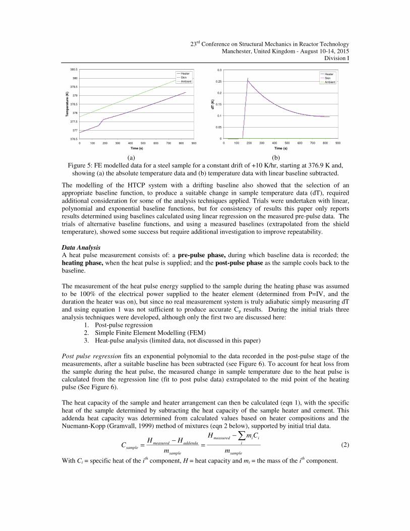
Finite element modelling of the system under both stable and drifting ambient temperature conditions
showed that there was a slight difference between the two measurement conditions (Figure 4 and 5). Thus
the dT of the sample with a drifting baseline (Figure 5b) stabilising at a temperature above dT=0, while
the dT for the sample with a stable baseline (Figure 4b) continues to decay towards dT=0. However, this
difference can be accounted for during the analysis of the pulse.
(a) (b)
Figure 4: FE modelled data for a steel sample at a stable ambient temperature of 376.9 K showing (a) the
absolute temperature data and (b) temperature data with linear baseline subtracted.
Model data: Stable Ambient Temperature
376.85
376.9
376.95
377
377.05
377.1
377.15
0 100 200 300 400 500 600 700 800 900
Time (s)
Te
mp
era
ture
(K
)
Heater
Skin
Ambient
Model data: Stable Ambient Temperature
0
0.05
0.1
0.15
0.2
0.25
0.3
0 100 200 300 400 500 600 700 800 900
Time (s)
dT
(K
)
Heater
Skin
Ambient
23rd
Conference on Structural Mechanics in Reactor Technology
Manchester, United Kingdom - August 10-14, 2015
Division I
(a) (b)
Figure 5: FE modelled data for a steel sample for a constant drift of +10 K/hr, starting at 376.9 K and,
showing (a) the absolute temperature data and (b) temperature data with linear baseline subtracted.
The modelling of the HTCP system with a drifting baseline also showed that the selection of an
appropriate baseline function, to produce a suitable change in sample temperature data (dT), required
additional consideration for some of the analysis techniques applied. Trials were undertaken with linear,
polynomial and exponential baseline functions, but for consistency of results this paper only reports
results determined using baselines calculated using linear regression on the measured pre-pulse data. The
trials of alternative baseline functions, and using a measured baselines (extrapolated from the shield
temperature), showed some success but require additional investigation to improve repeatability.
Data Analysis A heat pulse measurement consists of: a pre-pulse phase, during which baseline data is recorded; the
heating phase, when the heat pulse is supplied; and the post-pulse phase as the sample cools back to the
baseline.
The measurement of the heat pulse energy supplied to the sample during the heating phase was assumed
to be 100% of the electrical power supplied to the heater element (determined from P=IV, and the
duration the heater was on), but since no real measurement system is truly adiabatic simply measuring dT
and using equation 1 was not sufficient to produce accurate Cp results. During the initial trials three
analysis techniques were developed, although only the first two are discussed here:
1. Post-pulse regression
2. Simple Finite Element Modelling (FEM)
3. Heat-pulse analysis (limited data, not discussed in this paper)
Post pulse regression fits an exponential polynomial to the data recorded in the post-pulse stage of the
measurements, after a suitable baseline has been subtracted (see Figure 6). To account for heat loss from
the sample during the heat pulse, the measured change in sample temperature due to the heat pulse is
calculated from the regression line (fit to post pulse data) extrapolated to the mid point of the heating
pulse (See Figure 6).
The heat capacity of the sample and heater arrangement can then be calculated (eqn 1), with the specific
heat of the sample determined by subtracting the heat capacity of the sample heater and cement. This
addenda heat capacity was determined from calculated values based on heater compositions and the
Nuemann-Kopp (Gramvall, 1999) method of mixtures (eqn 2 below), supported by initial trial data.
sample
i
iimeasured
sample
addendameasuredsample
m
CmH
m
HHC
�−
=
−
= (2)
With Ci = specific heat of the ith component, H = heat capacity and mi = the mass of the i
th component.
376.5
377
377.5
378
378.5
379
379.5
380
380.5
0 100 200 300 400 500 600 700 800 900
Time (s)
Tem
pe
ratu
re (
K)
Heater
Skin
Ambient
Model data: Constant Drift (10 K per Hour)
0
0.05
0.1
0.15
0.2
0.25
0.3
0 100 200 300 400 500 600 700 800 900
Time (s)
dT
(K
)
Heater
Skin
Ambient

23rd
Conference on Structural Mechanics in Reactor Technology
Manchester, United Kingdom - August 10-14, 2015
Division I
(a) (b)
Figure 6: Temperature pulse measurement with a linear baseline subtracted for copper, showing (a) the
change in sample temperature, dT and (b) the dT data on a logarithmic scale, ln(dT).
The regression analysis of data in Figure 6 produced the following results for copper at room temperature:
Calculated Cp – from sample thermocouple: 471.2 J.kg-1
.K-1
Calculated Cp – from sample resistance thermometer: 389.8 J.kg-1
.K-1
The accepted specific heat capacity of copper at 293 K is 385 J.kg-1
.K-1
(Y.S. Toulokian, 1970) and as
noted above, the HTCP system derived values for the sample thermocouple and resistance heater differ
from the reference data by 22% and 1.2%, respectively.
Modelling and observed results showed that the post pulse data were best approximated with exponential
curves with polynomial exponents, where the polynomial order decreases as the temperature rises. The
exact polynomial order is sample and test specific. Figure 7 shows the decreasing order of polynomials
required as temperature increases.
(a) (b)
Figure 7: (a) Example of the modelled dT pulse data, with post pulse regression for at three temperature
(300 K (blue), 800 K (pink) and 1200 K (green)) and (b) ln(dT) post pulse data with the lowest order
polynomial fit with R2 = 1 to 4 DP.
The post pulse regression analysis was very dependent on the range over which the regression is taken,
attempts to automate the analysis proved difficult and the analysis had to be performed manually, with the
inherent issues of user inputs/interpretation. A design modification to use two temperature sensors may
resolve this issue but requires confirmation.
Finite element modelling (FEM) analysis was undertaken by fitting a simple 2-body finite element model
to the measured data by tuning the heat capacity of the sample and heat transfer coefficient between the
-0.2
0
0.2
0.4
0.6
0.8
1
1.2
1.4
1.6
1.8
0 200 400 600 800 1000 1200 1400
Time (s)
Tem
pera
ture
(K
)
SampleTC
Sample RST
Reg. Sample TC
Reg. Sample RST
0
0.1
0.2
0.3
0.4
0.5
0.6
0 100 200 300 400 500 600 700 800
Time (s)
dT
(K
)
300K
800K
1200K
dT absolute
curve fit 300K
curve fit 800K
curve fit 1200K
ln(dT-1200K) = -0.0098 t + 0.2071
R2 = 1.0000
ln(dT-800K)= 2.7173E-09 t3 - 2.5117E-06 t
2 -
5.2178E-03 t - 3.6540E-01
R2 = 1.0000E+00
ln(dT-300K) = 1.5154E-12 t4 - 1.9419E-10 t
3 +
5.5209E-09 t2 - 4.4513E-03 t -
4.8860E-01
R2 = 1.0000E+00
-8
-7
-6
-5
-4
-3
-2
-1
0
0 200 400 600 800
Time (S)
ln(d
T)
300 K model, post pulse data only
800 K model, post pulse data only
1200 K model, post pulse data only
Linear (1200 K model, post pulse dataonly)
Poly. (800 K model, post pulse data only)
Poly. (300 K model, post pulse data only)

23rd
Conference on Structural Mechanics in Reactor Technology
Manchester, United Kingdom - August 10-14, 2015
Division I
sample and heater. Figure 8 shows a copper sample heat pulse and a simple two body FEM analysis. The
FEM analysis of the data in Figure 8, produced a specific heat of Cp = 386 J.kg-1
.K-1
, reference data for
Copper Cp = 385 J.kg-1
.K-1
(Y.S. Toulokian, 1970) – clearly a good result.
Figure 8: Example of an analysis of a measured heat pulse for a copper sample using the two body model.
This technique is open to misinterpretation, by inputting impractical heat transfer coefficients. However,
the fact that the two-body model is optimized for more of the measured data means that it is a more robust
analysis technique than post-pulse regression.
The use of more complex models (splitting the sample/heater assembly into more than two nodes/bodies)
would improve the fit of the model but would introduce another unknown variable (thermal conductivity
of the sample). This would have a significant effect on the tuning of the model, since it would be possible
to produce identical heat pulse data with different specific heats using different thermal conductivities.
RESULTS & DISCUSSION After the initial testing was performed to refine the methodology and the analysis approach finalised, four
materials were selected to test the system. The variety of the samples also served to investigate the scope
of application for the HTCP system. The samples tested were in two forms: three of the four test samples
were cylindrical and the fourth was rectangular. Tables 1 and 2 below detail the test sample information:
Table 1: Cylindrical sample information
Sample
No. Material
Sample information
Diameter (mm) Length (mm) Mass (g)
1* Stainless Steel (Type 304) 7.905 18.244 6.235
2* Stainless Steel (Type 304) 7.905 14.353 5.785
3 Copper 8.536 17.259 7.900
4 Molybdenum 16.015 25.005 51.800 * sample 1 and 2 are the same piece of material with testing performed on the larger 6.235g sample (1) then the
sample reduced in size to produce the smaller 5.7859g sample (2)
Table 2: Rectangular sample information.
Sample
No. Material
Sample information
Width (mm) Depth (mm) Length (mm) Mass (g)
5 Graphite 5.935 5.802 15.325 0.983
Each sample underwent a range of heating and cooling rates between 1 K/hr and 10 K/hr and using
different heat pulse durations and powers, as well as recording data over varying pre-pulse and post pulse
durations. The results of the four materials are shown in Figures 9-12.

23rd
Conference on Structural Mechanics in Reactor Technology
Manchester, United Kingdom - August 10-14, 2015
Division I
��� ���
Figure 9: Measured specific heat capacity of copper using (a) post pulse regression on both the sample
thermocouple (blue) and the platinum resistance thermometer (red), and (b) using FEM analysis. Standard
reference data taken from (Y.S. Toulokian, 1970)
�
��� ���
Figure 10: Measured specific heat capacity of stainless steel samples 1 and 2, using (a) post pulse
regression and (b) using FEM analysis. Standard reference data taken from (Y.S. Toulokian, 1970)
The conventional regression analysis for both the copper (Figure 9a) and the stainless steel
(Figure 10a) samples generally gave specific heats very comparable with the literature (Y.S.
Toulokian, 1970). However, it should be noted that above ~900K there was considerable scatter in the
values obtained for the stainless steel (Figure 10a) and this was thought to be associated with the sample
heater failing.
During the measurement of the graphite sample (Figure 11), a seal on the vacuum system failed, and the
sample oxidised when the temperature exceed 480 K, with the sample finally failing at 540 K. At the
temperature oxidation started, the measured Cp data begins to deviate from the reference data as would be
expected. If the heat capacity to specific heat conversion equation (eqn 2) is corrected for mass loss
(assuming linear mass loss due to oxidation with respect to temperature/time) the corrected measured Cp
0
100
200
300
400
500
600
700
292.5 293.0 293.5 294.0 294.5 295.0
Specific
Heat (J
.kg
-1.K
-1)
Temperature (K)
Cp TC
Cp RST
Cu Std Refrence data*330
340
350
360
370
380
390
400
410
420
293 293.5 294 294.5 295
Specific
Heat (J
.kg
-1.K
-1)
Temperature (K)
Copper FEM analysis
Copper Reference data*
0
100
200
300
400
500
600
700
800
900
1000
280 480 680 880 1080 1280
Specific
Heat (J
.Kg-1
.K-1
)
Temperature (K)
S.Steel 1, 10 K/hr-RST-heating
S.Steel 1, 10 K/hr-RST-cooling
S.Steel 1, 6 K/hr-RST heating
S.Steel 2, 10 K/hr-RST
Std Reference data
0
100
200
300
400
500
600
700
800
280 380 480 580 680
Specific
Heat (J
.kg
-1K
-1)
Temperature (K)
Stainless Steel, FEM Analysis
Std Reference Data [ref]

23rd
Conference on Structural Mechanics in Reactor Technology
Manchester, United Kingdom - August 10-14, 2015
Division I
once again agrees reasonably with the reference data (orange markers on Figure 11a). Here the FEM
analysis of the data appears to have been particularly successful (Figure 11b), with both the value and
shape of the specific heat variation well captured, up until the oxidation problem was reached.
���� ����
Figure 11: Measured specific heat capacity of graphite, using (a) post pulse regression and (b) using FEM
analysis.. Standard reference data taken from (Y.S. Toulokian, 1970)
(a) (b)
Figure 12: Measured specific heat capacity of molybdenum, using (a) post pulse regression and (b) using
FEM analysis. Standard reference data taken from (Y.S. Toulokian, 1970)
As with the other materials, the specific heat values obtained for the molybdenum (Figure 12) generally
compared well with the literature (Y.S. Toulokian, 1970). There was some scatter in the data obtained by
both the regression and FEM analyses approaches and the regression data gave the more reliable fit to the
literature.
The limiting factor on most measurements (i.e. maximum temperature at which a measurement was
made) was component failure, usually the support wires or sample heater connections failing. These
failures not only limited the testing but results in increased scatter on the data prior to failure. There is
clearly work to be done in enhancing the robustness of the current experimental arrangement.
0
200
400
600
800
1000
1200
1400
280 330 380 430 480 530
Specific
Heat (J
.kg
-1.K
-1)
Temperature (K)
Measured Graphite (corrected)
Measured Graphite (un-corrected)
Std Refernce Data [ref] 0
200
400
600
800
1000
1200
1400
280 330 380 430 480 530
Specific
Heat (J
.kg
-1K
-1)
Temperature (K)
Graphite, FEM Analysis
Std Reference Data [ref]
0
50
100
150
200
250
300
350
280 480 680 880 1080 1280
Cp (
J.K
g-1
.K-1
)
Temperature (K)
Measure Cp - stable
Measured Cp- Drift 10K/hr
Std Reference Data [ref]
0
50
100
150
200
250
300
350
280 480 680 880
Specific
Heat (J
.kg
-1.K
-1)
Temperature (K)
Molybdenum, FEM AnalysisStd Reference Data [ref]

23rd Conference on Structural Mechanics in Reactor Technology
Manchester, United Kingdom - August 10-14, 2015
Division I
The data recorded and analysed for all four samples compares well to standard reference data over the
temperature range measured (Figures 9 to 12), even showing good repeatability with multiple
measurements using varying measurement parameters e.g. heating rates, sample mass, pulse duration,
sample heater power, etc. (Figure 10). The new FE modelling analysis technique produced data that
compared well with both reference data and the results of the more traditional regression analysis, and
shows promise for further development. However, as the system currently stands the results show more
scatter than would be observed with DSC measurements but the physical advantages (size, geometry,
surface finish) of the HTCP make it applicable for some materials and applications. There are also further
developments that could enhance the HTCP system and improve the reliability of measurements,
including engineering improvements and analysis methodologies.
SUMMARY A high temperature quasi-adiabatic calorimeter (HTCP) has been successfully developed, along with the
required novel data analysis techniques.
The specific heat data produced by the HTCP system for the four materials were in good agreement with
the reference data. Of the four samples measured the smallest sample (graphite) producing the most
accurate data (until oxidation of the sample invalidated the measurement).
The commissioning testing, while not complete, has shown that a wide range of sample sizes, geometries
and types are can be measured, unlike other Cp measurement approaches, and it has the potential for a
high level of accuracy even in non-ideal conditions. However, there remains considerable development
required to automate the technique and improve repeatability.
REFERENCES
������ ����Cherneko, V., Kokorin, V. & Vitenko, I., 1994. Brief Communication: Properties of ribbon made from
shape memory alloy Ni2MnGa by quenching from liquid state. Smart Mater Struct. 3, pp. 80-82.
Gramvall, G., 1999. Thermal Phsyical Properties of Materials. North-Holland: Elsevier Science B.V..
IRCP, 1996. Chapter 1: Specific heat measurement techniques. In: International materials database.
s.l.:IRCP, p. i to xi.
Khovailo, V. V. et al., 2001. On order-disorder (L21/B2’) phase transition in Ni2+xMn1-xGa Heusler
alloys. Physica Status Solidi A-Applied Research, 183, pp. R1-R3.
Kirkham, M., 2014. High temperature specific heat capacity measuement of Ni2-XMn1+XGa, s.l.:
Loughbourough University.
Nernst, W., 1911. The energy content of solids. Ann Physic 36, pp. 395-439.
Neumann, K. et al., 2009. The Average Valence Electron Number: Is it a relevant parameter for
Ni2MnGa Alloys?. MRS Proceedings, Volume 1200.
Reece, P., 2007. Progress in Smart Materials ans Structures, s.l.: Nova Publishing.
V. Recarte, J. P.-L. V. S.-A. a. J. R.-V., 2012. Dependence of the martensitic transformation and magnetic
transition on the atomic. Acta Materialia, Vol 60, Issue 5, p. 937–1945.
Y.S. Toulokian, R. P. C. H. a. P., 1970. Thermophsycal properties of matter, The TPRC Data Series. New
York and Washington: IFI/Plenum.


