Hybrid Digital-Analog Source-Channel Coding withOne-to-Three Bandwidth Expansion

Ahmad Abou Saleh, Fady Alajaji, and Wai-Yip Chan

Abstract—We consider the problem of bandwidth expansionfor lossy joint source-channel coding over a memoryless Gaussianchannel. A low delay 1:3 bandwidth expansion hybrid digital-analog coding system, which combines a scalar quantizer anda 1:2 nonlinear analog coder, is proposed. It is shown thatour proposed system outperforms the 1:3 generalized hybridscalar quantizer linear coder in terms of signal-to-distortion ratio(SDR). A lower bound on the system SDR is also derived.

I. INTRODUCTION

The traditional approach for analog source transmission

is to use separate source and channel coders. This separa-

tion is optimal given infinite delay and complexity in the

coders [1]. In practice, joint source-channel coding (JSCC)

can achieve better performance when delay and complexity are

constrained. A common approach for JSCC design is to jointly

optimize the components of a tandem system with respect to

the channel and source characteristics. Another approach based

on non-linear analog mapping is treated in [2]–[5].

With the increasing popularity of wireless sensors networks,

reliable transmission with delay and complexity constraints

is more relevant than ever. A sensor node communicates

its sensed field information to a fusion center over a noisy

wireless channel. In this paper, we focus on low delay and

low complexity lossy JSCC by proposing a 1:3 bandwidth

expansion scheme based on combining a scalar quantizer with

a 1:2 nonlinear analog coder operating on the quantization

error. The proposed hybrid digital-analog scheme is shown to

be suitable for wireless sensor networks.

The hybrid scalar quantizer linear coder (HSQLC) provides

a dimension expansion of rate R = 2 [6]. This scheme uses

pulse amplitude modulation to send a scalar quantizer output

on one channel, and linear uncoded analog transmission of

the quantization error on another channel. For rates larger

than two (R > 2), Coward suggested to repeatedly quantize

the error from the previous quantization step and finish the

last step with a linear coder [7]. Recently, a similar system

was studied in [8], referred to as ”generalized HSQLC”. For

reference, we compare the proposed system to the generalized

HSQLC. Similar hybrid systems based on splitting the source

into a quantization part and a quantization error part were also

proposed in [9]. These schemes, however, use long channel

block codes for the quantization part, thus incurring large

This work was supported in part by NSERC of Canada.A. Abou Saleh and W-Y. Chan are with the Department of Electrical and

Computer Engineering, Queen’s University, Kingston, ON, K7L 3N6, Canada.F. Alajaji is with the Department of Mathematics and Statistics and the

Department of Electrical and Computer Engineering, Queen’s University,Kingston, ON, K7L 3N6, Canada.

delay and complexity and making them not comparable with

our proposed low delay scheme. The rest of the paper is

organized as follows. In Section II, we describe a Shannon-

Kotel’nikov mapping using the 1:2 Archimedes’ spiral. Sec-

tion III describes the system model and optimization. A lower

bound on the system signal-to-distortion ratio (SDR) is derived

in Section IV. Simulation results are included in Section V.

Finally, conclusions are drawn in Section VI.

II. A SHANNON-KOTEL’NIKOV MAPPING

In this section, a 1:2 Archimedes’ spiral mapping is de-

scribed for both uniform and Gaussian memoryless sources.

Bandwidth expansion is performed by mapping each source

sample x ∈ R to a two-dimensional channel symbol, which is

a point on the double Archimedes’ spiral, given by [5]

s(x) =

[z1(x)z2(x)

]=

1

π

[sgn(x)Δϕ(x) cosϕ(x)sgn(x)Δϕ(x) sinϕ(x)

](1)

where sgn(·) is the signum function, Δ is the radial dis-

tance between any two neighboring spiral arms, and ϕ(x) =√6.25|x|/Δ is a stretching bijective function. For a given

channel signal-to-noise ratio (CSNR) defined as P/σ2N , where

P and σ2N are the average channel power and noise variance,

respectively, the radial distance Δ is optimized to minimize

the total distortion by solving the following unconstrained

optimization problem

Δopt = argminΔ

[ε2wn(Δ) + ε2th(Δ)] (2)

where ε2wn and ε2th are, respectively, the average weak noise

and threshold distortion under maximum likelihood (ML)

decoding. For a uniform source on the interval [−a, a], where

a > 0, the average weak noise distortion is [5]

ε2wn =σ2N

α2(3)

where α is a gain factor related to the average channel power

constraint P given by

P =1

2

∫ a

−a

||s(αx)||2fX(x)dx (4)

where fX(x) is the probability density function (pdf) of the

source X . The threshold distortion for a uniform source is

ε2th = 2a2(1− erf

(Δ

2√2σN

))(4a

3+

π4η2Δ2

α2a+

4π2ηΔ

α

)(5)

where erf(·) is the Gaussian error function, and η = 0.16.

Hence, the calculated performance of the 1:2 spiral mapping

under ML decoding is SDR = σ2X/(ε2wn + ε2th), where σ2

X is

the source variance. For a Gaussian source, the expression for

the threshold distortion is derived in [5].

At the receiver side, we use the optimum minimum mean

square error (MMSE) decoder instead of the ML decoder

used in [5]. MMSE decoding has been shown to achieve

a substantial performance improvement over ML decoding

at low CSNRs under 2:1 bandwidth reduction [10]. For 1:2

bandwidth expansion, the MMSE decoding rule can be written

as follows

x = E[X|z1, z2] =∫

xp(x|z1, z2)dx =

∫xp(z1, z2|x)p(x)dx∫p(z1, z2|x)p(x)dx

(6)

where {zi}i=1,2 = zi + ni are the received channel outputs.

For independent and identically distributed (i.i.d.) Gaussian

noise ni, we have p(z1, z2|x) = p(z1|x)p(z2|x), where

p(zi|x) = 1√2πσN

e− (zi−zi(x))2

2σ2N , i = 1, 2 (7)

and zi(x) is given by (1). To make the decoder implemen-

tation computationally efficient, we devise a decoder based

on quantization and table-lookup. This is done by uniform

quantization of the output of the channel z ∈ R2 and looking

up the decoded value x for each quantization bin in a table.

As shown in Fig. 1, the performance of the spiral mapping

with uniform source is at most 8 dB below the theoretical limit.

This is comparable to the case of Gaussian source [5]. It can be

noticed that the performance of the 1:2 bandwidth expansion

system with MMSE decoder is close to the performance of

the block pulse amplitude modulation (BPAM) [11] at low

CSNRs (≤ 10 dB), and to the 1:2 bandwidth expansion system

with ML decoding at high CSNRs (> 10 dB). Since it is

intractable to find an analytical expression for the system

performance under MMSE decoding, we use the following

approximation to represent it

Dexp =

{DBPAM =

(σXσN

P+σ2N

)2 (σ2N + P 2

2

), CSNR ≤ 10dB

DML = ε2wn + ε2th, otherwise(8)

where DBPAM and DML are, respectively, the distortion from

the 1:2 BPAM and 1:2 spiral expansion under ML decoding.

In Fig. 1, this is given by the dashed curve for CSNR≤ 10dB

and by the solid curve (with pluses) for CSNR> 10dB. Similar

results are also obtained for Gaussian source.

III. SYSTEM MODEL

A. System Structure

In this section, we assume a Gaussian source X with

variance σ2X to be transmitted over a power limited, discrete

time, and continuous amplitude channel with additive white

Gaussian noise n ∼ N (0, σ2N ). We propose a 1:3 bandwidth

expansion system that consists of a scalar quantizer and a

1:2 dimension expansion using Archimedes’ spiral, as shown

in Fig. 2. The proposed system works as follows. A source

symbol X is first quantized using an L-level quantizer Q(.).

The quantizer uses a set of decision intervals Di = (di, di+1)

0 5 10 15 20 25−10

0

10

20

30

40

50

CSNR [dB]

SD

R [d

B]

1:2 bandwidth expansion with MMSE decoder1:2 bandwidth expansion with ML decoderLinear system (BPAM)Theoretical limit (OPTA)

Fig. 1. Performance of the 1:2 bandwidth expansion system for a uniformlydistributed source over [-1,1] using the Archimedes’ spiral. The optimalperformance theoretically attainable (OPTA) SDR=σ2

X/D, where D is thetotal distortion, is plotted for a memoryless Gaussian source which representsa lower bound on OPTA SDR for all other sources. The linear system SDRis also plotted.

Fig. 2. System Model.

with d0 = −∞ and dL = +∞. It returns both the index

i and the representation level A = ai, i = {0, . . . , L − 1}.The index i is represented by the channel input Y1 = ci.The quantization error B = X − A is mapped to a two-

dimensional channel symbol using the 1:2 Archimedes’ spiral.

The system is optimized to minimize the mean square error

(MSE) E[(X − X)2] while satisfying the average channel

power constraint P

1

3

{E[Y 2

1 ] +

∫||s(αb)||2fB(b)db

}≤ P (9)

where α is the gain factor, and fB(b) is the pdf of the

quantization error B. At the receiver, we use optimal decoders

for both the received quantized symbol and quantization error.

The MMSE decoder introduced in Section II is used on the

quantization error, and the quantized symbol is decoded as

β1(y1) = E[A|y1] =∑L−1

i=0 aiP (ai)e− (y1−ci)

2

2σ2N

∑L−1i=0 P (ai)e

− (y1−ci)2

2σ2N

(10)

where P (ai) is the probability that A = ai. Note that table-

lookup can be used to reduce complexity. We also use a mid-

tread uniform quantizer, so that only spacing between levels

need to be specified(i.e., ai =

(i− (L− 1)/2

)δa, ci = Kai

for i ∈ 0, ..., L− 1, dj =(j − L/2

)δd for j ∈ 1, ..., L− 1,

and L is an odd number).

The distribution of the quantization error B is given by

fB(b) =L−1∑i=0

fA,B(ai, b) (11)

where fA,B(ai, b) can be expressed as follows

fA,B(ai, b) =

{fX(b+ ai), b ∈ (di − ai, di+1 − ai)

0, Otherwise.

(12)

Using (11), the average channel power constraint in (9)

becomes

1

3

{σ2Y1

+αΔ

π2η

L−1∑i=0

(∫ di+1

di

|x− ai|fX(x)dx

)}≤ P (13)

where σ2Y1

is the variance of the channel input Y1.

B. System Optimization

The overall MSE E[(X−X)2] can be broken up as follows

MSE = MSEq + MSEexp (14)

where MSEexp is the distortion in decoding B, and MSEq is

the distortion in decoding A, given by

MSEq = E[(A− A)2] = E[(A− β1(C(A) + n))2]

=

∫ +∞

−∞

L−1∑i=0

(ai − β1(ci + n))2P (ai)fN (n)dn

(15)

where fN (n) is the pdf of the Gaussian noise.

We minimize numerically the MSE with respect to the

quantizer parameters (δa, K, δd), spiral parameter Δ, and

α. For a given amount of power P1 assigned to Y1, the

quantizer parameters are found by minimizing MSEq using

the line search strategy. The optimization is performed for

increasing channel noise levels. As initial condition for the

optimization, the result for the previous noise level is used. We

also impose additional solution constraints that the parameters

are real positive-valued and σ2Y1

is equal to the power assigned

to Y1.

By setting δa = δd, the interval (di − ai, di+1 − ai) =( − δd2 ,+

δd2

)in (12) is fixed for i = 1, . . . , L − 2. For low

CSNRs, one can argue that the pdf fB(b) can be approximated

by a Gaussian distribution, since minimizing MSEq will make

δd large. For high CSNRs, B fits well a uniform distribution

by the fact that δd is relatively small with respect to σX and the

overload probability is negligible. For the sake of simplicity,

the spiral optimization (i.e., finding Δ) is conducted assuming

that the quantization error B fits well either a Gaussian or

a uniform distribution. Hence, results from Section II can be

used; (Δ, α) are optimized using (2) while (13) is satisfied

with equality, and MSEexp is calculated in a similar way to (8).

The design algorithm is formally stated below.

1) Choose some initial values for (δa,K, L).

2) Set i = 0, the overall MSE D(0) =∞, Dbest =∞, and

the power assigned to Y1, P1 = βP , 0 ≤ β ≤ 3.

3) Let N be the noise variance level for which the system

should be optimized. Set N ′ to correspond to a less noisy

channel.

4) Set i← i+ 1.

5) Find the optimal quantizer parameters (δa,K) for N ′

by minimizing (15) under the constraint σ2Y 1 = P1.

6) If N ′ ≥ N go to Step 7. Otherwise set N ′ ← γN ′,γ > 1, and go to Step 5 using the current parameters as

initialization for the new optimization.

7) Optimize (Δ, α) using (2) while (13) is satisfied with

equality.

8) Calculate MSEexp using (8), and D(i) using (14).

9) If Dbest > D(i), set Dbest ← D(i), and R ←(δa,K,Δ, α,Dbest, P1).

10) If P1 > εP , set P1 ← P1 − λP , and go to Step 4.

11) Return R.

In our simulations, we used L = 35, β = 1, the initial noise

level N ′ is set to correspond to a channel with CSNR = 30dB, γ = 100.5 which correspond to a 5 dB decrease in CSNR

level, and ε = λ = 0.1. Note that we also conducted some

simulations for P1 > P (i.e., β > 1).

IV. SYSTEM LOWER BOUND ON THE SDR

In this section, we derive a lower bound on the proposed

system SDR following the approach of [8]. For this bound,

we assume (suboptimal) ML decoding for recovering both the

quantized symbol and quantization error.For the quantized symbol, the system works as follows. At

the encoder side, the quantized symbol is scaled by a gain fac-

tor K to satisfy the power constraint and transmitted through

the channel. At the receiver, the channel output is rescaled

using 1/K and ML decoder, which is a minimum distance

estimator, is applied on the rescaled signal y1 = ai+ n, where

n ∼ N (0, (σN

K )2). The error in decoding the quantized value

can be expressed as follows

E[(A− A)2] = δ2a

L−1∑i=0

P (ai)

L−1∑j=0

(j − i)2Pi,j

≤ δ2aL

L−1∑m=1

m2Pm (16)

where m = |j − i|, and Pm = Pi,j is the probability of

receiving aj when ai is transmitted, given by

Pi,j = Q

((|j − i| − 1/2)δa

σN

K

)−Q

((|j − i|+ 1/2)δa

σN

K

)(17)

where j = 2, ..., L− 2, and Q(x) is the Gaussian Q-function

which can be upper bounded for x ≥ 0 as

Q(x) =1√2π

∫ ∞

x

e−τ2/2dτ ≤ 1

2e−x2/2. (18)

Using (18) and dropping the second term in (17), the transition

probability Pi,j can be upper bounded by

Pi,j ≤ 1

2exp

(−K2 (m− 1/2)2δ2a

2σ2N

). (19)

Thus (16) can be expressed as follows

E[(A− A)2] ≤ δ2aL

2

L−1∑m=1

m2 exp

(− (Kδa)

2(m− 1/2)2

2σ2N

)

≤ δ2aL

2exp

(−K2δ2a

8σ2N

)

+δ2aL

2

L−1∑m=2

m2 exp

(− (Kδa)

2m

2σ2N

)(20)

where we have used the fact that (m−1/2)2 > m for m ≥ 2.

The summation can be bounded to obtain an upper bound on

the distortion from decoding the quantized symbol

�∑m=2

m2zm ≤�∑

m=1

m2zm =z

(1− z)3(1 + z − (�+ 1)2z�

+(2�2 + 2�− 1)z�+1 − �2z�+2)

(21)

where z = exp(− (Kδa)

2

2σ2N

), and � = L− 1.

The distortion from decoding B is bounded by

E[(B − B)2] ≤ ε2wn + ε2th (22)where ε2wn and ε2th are, respectively, the weak noise and thresh-

old distortion given by (3) and (5). Adding (20) and (22) gives

an upper bound on the end-to-end distortion, thus yielding a

lower bound on the system SDR.V. NUMERICAL RESULTS

In this section, we assume an i.i.d. Gaussian source X with

variance σ2X =1. The power allocated to Y1, P1, is chosen

to maximize the overall MSE in (14). For high CSNRs, it is

noticed that P1 = P , while for low CSNRs, assigning lower

power to Y1 gives the best performance. This can be explained

by the fact that at low CSNRs, the optimization decreases the

number of effective quantization levels (i.e., δd is large) in

order to minimize the decoding error. This means that the

probability of the quantized value being nonzero is low. Two

other systems are considered and compared to our proposed

system: 1) the optimal linear system (1:3 BPAM) which is

the best possible linear solution [11], and 2) a 1:3 generalized

HSQLC introduced in [8]. Note that the generalized HSQLC

parameters are optimized for the given CSNR level. This is

done by searching for the quantization resolution that gives the

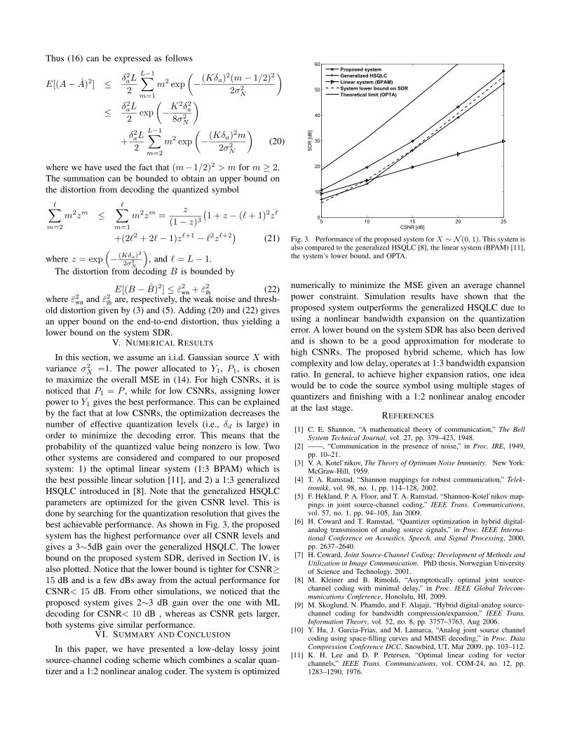
best achievable performance. As shown in Fig. 3, the proposed

system has the highest performance over all CSNR levels and

gives a 3∼5dB gain over the generalized HSQLC. The lower

bound on the proposed system SDR, derived in Section IV, is

also plotted. Notice that the lower bound is tighter for CSNR≥15 dB and is a few dBs away from the actual performance for

CSNR< 15 dB. From other simulations, we noticed that the

proposed system gives 2∼3 dB gain over the one with ML

decoding for CSNR< 10 dB , whereas as CSNR gets larger,

both systems give similar performance.VI. SUMMARY AND CONCLUSION

In this paper, we have presented a low-delay lossy joint

source-channel coding scheme which combines a scalar quan-

tizer and a 1:2 nonlinear analog coder. The system is optimized

5 10 15 20 250

10

20

30

40

50

60

CSNR [dB]

SD

R [d

B]

Proposed systemGeneralized HSQLCLinear system (BPAM)System lower bound on SDRTheoretical limit (OPTA)

Fig. 3. Performance of the proposed system for X ∼ N (0, 1). This system isalso compared to the generalized HSQLC [8], the linear system (BPAM) [11],the system’s lower bound, and OPTA.

numerically to minimize the MSE given an average channel

power constraint. Simulation results have shown that the

proposed system outperforms the generalized HSQLC due to

using a nonlinear bandwidth expansion on the quantization

error. A lower bound on the system SDR has also been derived

and is shown to be a good approximation for moderate to

high CSNRs. The proposed hybrid scheme, which has low

complexity and low delay, operates at 1:3 bandwidth expansion

ratio. In general, to achieve higher expansion ratios, one idea

would be to code the source symbol using multiple stages of

quantizers and finishing with a 1:2 nonlinear analog encoder

at the last stage.REFERENCES

[1] C. E. Shannon, “A mathematical theory of communication,” The BellSystem Technical Journal, vol. 27, pp. 379–423, 1948.

[2] ——, “Communication in the presence of noise,” in Proc. IRE, 1949,pp. 10–21.

[3] V. A. Kotel’nikov, The Theory of Optimum Noise Immunity. New York:McGraw-Hill, 1959.

[4] T. A. Ramstad, “Shannon mappings for robust communication,” Telek-tronikk, vol. 98, no. 1, pp. 114–128, 2002.

[5] F. Hekland, P. A. Floor, and T. A. Ramstad, “Shannon-Kotel’nikov map-pings in joint source-channel coding,” IEEE Trans. Communications,vol. 57, no. 1, pp. 94–105, Jan 2009.

[6] H. Coward and T. Ramstad, “Quantizer optimization in hybrid digital-analog transmission of analog source signals,” in Proc. IEEE Interna-tional Conference on Acoustics, Speech, and Signal Processing, 2000,pp. 2637–2640.

[7] H. Coward, Joint Source-Channel Coding: Development of Methods andUtilization in Image Communication. PhD thesis, Norwegian Universityof Science and Technology, 2001.

[8] M. Kleiner and B. Rimoldi, “Asymptotically optimal joint source-channel coding with minimal delay,” in Proc. IEEE Global Telecom-munications Conference, Honolulu, HI, 2009.

[9] M. Skoglund, N. Phamdo, and F. Alajaji, “Hybrid digital-analog source-channel coding for bandwidth compression/expansion,” IEEE Trans.Information Theory, vol. 52, no. 8, pp. 3757–3763, Aug 2006.

[10] Y. Hu, J. Garcia-Frias, and M. Lamarca, “Analog joint source channelcoding using space-filling curves and MMSE decoding,” in Proc. DataCompression Conference DCC, Snowbird, UT, Mar 2009, pp. 103–112.

[11] K. H. Lee and D. P. Petersen, “Optimal linear coding for vectorchannels,” IEEE Trans. Communications, vol. COM-24, no. 12, pp.1283–1290, 1976.