Hydraulic Design of an Overland Flow
Distribution System Using Lateral Weirs
by
Victor M. Vargas Lugo
A report submitted in partial fulfillment of the requirements for the degree of
MASTER OF ENGINEERING
in
CIVIL ENGINEERING
UNIVERSITY OF PUERTO RICO
MAYAGÜEZ CAMPUS
2014
Approved by:
Walter F. Silva Araya Ph.D.
President, Graduate Committee
__________________
Date
Raúl E. Zapata López, Ph. D.
Member, Graduate Committee
__________________
Date
Jorge Rivera Santos, Ph. D.
Member, Graduate Committee
__________________
Date
Francisco Monroig Saltar, Ph. D.
Representative Graduate Studies
Ismael Pagán Trinidad, M.S.C.E.
Chairperson of the Department
__________________
Date
__________________
Date

ii
ABSTRACT
Jobos Bay Estuary Research Reserve (JBNERR) is located Salinas in Puerto Rico. Mar
Negro wetland is the biggest mangrove forest in the area located at the south boundary of
JBNERR. The north side of the Reserve has been used for agricultural activities since the
Spanish Colonial times. Since 1993 the mangrove started to diminish and its mortality was
promoted by antropogenic activities.
This project consisted of: 1) Study of the hydrologic and hydraulic conditions existing at
the north side of JBNERR; 2) Hydraulic design of channels with a system of weirs to re-direct
irrigation and rain runoff to a parcel of land before discharging into Mar Negro. This water
distribution will control surface runoff, reduce surface erosion, and improve the quality of runoff
waters discharging into the mangrove. The project analysis was prepared using SWMM
software, field work, and historical rainfall data to get the details features of the study area.
Keywords: Jobos Bay, JBNEER, Hydrology, Hydraulics, Side Wiers, Wiers, SWMM,
Watershed, Channel, Riprap, ArcGIS, AutoCAD, Mangroves, Rainfall, Transitions
iii
RESUMEN
La Reserva de Investigación Estuarina Bahía de Jobos (JBNERR) se encuentra Salinas,
Puerto Rico. Mar Negro es el mayor bosque de manglar ubicado al sur de JBNERR. El área norte
de la Reserva se ha utilizado para actividades agrícolas desde los tiempos coloniales españoles.
Desde 1993, el manglar comenzó a disminuir y su mortandad ha sido promovida por actividades
antropogénicas.
Este proyecto consistió en: 1) Estudio de las condiciones hidrológicas e hidráulicas
existentes al norte de JBNERR; 2) Diseño hidráulico de canales con un sistema de vertedores
para redirigir las escorrentías por riego y de lluvia a una parcela antes de alcanzar al mar Negro.
Esta distribución de agua controlará la escorrentía superficial, reducirá la erosión, y mejorará la
calidad del agua de escorrentía que alcance el manglar. El análisis del proyecto se preparó
utilizando SWMM, trabajo de campo, y datos históricos de precipitación para obtener los
detalles del área de estudio.
Palabras claves: Bahía de Jobos, JBNEER, Hidrología, Hidráulicas, Vertedores Laterales,
Vertedor, SWMM, Cuenca, Canal, Riprap, ArcGIS, AutoCAD, Manglar, Precipitación,
Transición.

iv
Copyright © 2014 by Victor M. Vargas Lugo All rights reserved. Printed in the United States of
America. Except as permitted under the United States Copyright Act of 1976, no part of this
publication may be reproduced or distributed in any form or by any means, or stored in a data
base or retrieved system, without the prior written permission of the publisher.

v
Dedicado a:
A Dios sobre todas las cosas.
Mi madre Lucia Lugo por su apoyo incondicional.
La novia eterna, Lizbeth por su apoyo, ayuda y comprensión.
A mi mentor, el Dr. Walter Silva por su paciencia, enseñanza y guiarme en este proyecto.
Dedicated to:
God above all things.
My mother Lucia for their unconditional support.
The eternal girlfriend, Lizbeth for their support, help and understanding.
To my mentor, Dr. Walter Silva for his patience, teaching and guiding me in this project.

vi
ACKNOWLEDGMENTS
The author would like to express sincere thanks to Dr. Walter F Silva Araya, for his support,
patience, and encouragement throughout the graduate studies. Also, I want to appreciate the
opportunity to work for the Puerto Rico Water Resources and Environmental Research Institute.
I want acknowledge the people who contributed substantially to this project: Roy Ruiz Velez,
Assistant Researcher Water Resources; Jesenia Carrero Lorenzo, Administrative Assistant from
Puerto Rico Water Resources and Environmental Research Institute; Rubén C. Soto Maisonet,
Surveying and Civil Engineering Student at UPRM; Angel Dieppa, Puerto Rico Department of
Natural and Environmental Resources-Jobos Bay National Estuarine Research Reserve who
assisted with data collection at the site.
Finally I would like to thanks Mrs. Carmen González Sifonte, Jobos Bay National Estuarine
Research Reserve Manager, for her cooperation and assistance in Jobos area. Also, for being the
person on whose concern for Jobos Bay protection, this project could be performed.

vii
TABLE OF CONTENT
Page
List of Tables ................................................................................................................................. x List of Figures .............................................................................................................................. xii Figures in Appendix .................................................................................................................... xv
List of Acronyms ........................................................................................................................ xvi
CHAPTER 1 INTRODUCTION ................................................................................................. 1
1.1 PROBLEM STATEMENT ........................................................................................................... 2
1.2 SCOPE AND OBJECTIVE OF THE STUDY ................................................................................... 6
CHAPTER 2 STUDY AREA DESCRIPTION .......................................................................... 7
2.1 LOCATION AND PHYSIOGRAPHIC REGION ........................................................................... 7
2.2 EXISTING TOPOGRAPHY ......................................................................................................... 9
2.3 CLIMATE .............................................................................................................................. 10
2.4 GEOLOGY ............................................................................................................................. 10
1.1 AGRICULTURAL ACTIVITIES ................................................................................................. 13
CHAPTER 3 MODEL DESCRIPTION ................................................................................... 14
3.1 RUNOFF AND HYDRAULIC SIMULATION ............................................................................... 14
3.2 CONCEPTUAL MODEL. ......................................................................................................... 15
3.2.1 HYDROLOGICAL COMPUTATIONS ................................................................................... 16
3.2.2 INFILTRATION ....................................................................................................................... 17
3.2.3 HYDRAULICS COMPUTATIONS ......................................................................................... 18
3.2.4 FLOW ROUTING METHODS ................................................................................................ 19
CHAPTER 4 HYDROLOGY .................................................................................................... 22
4.1 STORM RAINFALL EVENTS ................................................................................................... 22
4.2 WATERSHED ........................................................................................................................ 22
4.3 OVERLAND FLOW ROUGHNESS ............................................................................................ 25
4.4 HYDROLOGIC ABSTRACTION ................................................................................................ 26
4.5 HISTORICAL RAINFALL ........................................................................................................ 31
4.6 AGRICULTURAL IRRIGATION ................................................................................................ 32
4.7 SWMM HYDROLOGY SETTING AND MODELING .................................................................. 33
viii
4.8 HYDROLOGIC ANALYSIS ...................................................................................................... 34
4.8.1 RUNOFF BY CN METHOD .................................................................................................... 35
4.8.2 IRRIGATION DATA ................................................................................................................ 35
CHAPTER 5 HYDRAULICS .................................................................................................... 37
5.1 GENERAL HYDRAULIC PROCEDURES ................................................................................... 38
5.2 CHANNELS CHARACTERISTICS AND SIDE WEIRS DESIGN ..................................................... 39
5.3 CHANNEL LINING ................................................................................................................. 41
5.4 RIPRAP – LINING CHANNEL DESIGN PROCEDURES ............................................................... 43
5.4.1 RIPRAP DESIGN CRITERIA .................................................................................................. 43
5.4.2 RESULTS AND DISCUSSION ............................................................................................... 48
5.5 CHANNEL BEND .................................................................................................................... 50
5.6 CHANNEL TRANSITION ......................................................................................................... 54
5.7 SIDE WEIRS DESIGN ............................................................................................................. 71
5.7.1 SPILLFLOW CALCULATIONS ............................................................................................. 78
5.7.2 RESULTS .................................................................................................................................. 79
5.7.3 SIDE WEIR PROFILE .............................................................................................................. 85
5.7.4 VERIFICATION OF WATER SURFACE PROFILE .............................................................. 86
5.8 RECOMMENDED CHANNEL DIMENSIONS .............................................................................. 91
CHAPTER 6 PROJECT REPRESENTATION IN SWMM .................................................. 94
6.1 MODELING DESIGN .............................................................................................................. 95
6.2 SENSITIVITY ANALYSIS ........................................................................................................ 96
CHAPTER 7 DESIGN ALTERNATIVES ............................................................................. 110
CHAPTER 8 ANALYSIS AND DISCUSION ........................................................................ 114
CHAPTER 9 DESIGN RECOMENDATIONS...................................................................... 121
9.1 LAND SURVEY ................................................................................................................... 121
9.2 CUT AND FILL .................................................................................................................... 125
9.3 COST ESTIMATE ................................................................................................................. 133
BIBLIOGRAPHY……………………………………………………………………………. 138
APPENDIX ................................................................................................................................ 144
ix
APPENDIX A CURVE NUMBER TABLES ................................................................................. 144
APPENDIX B MAXIMUM 24-HR RAINFALL FOR EACH YEAR OF ANALYSIS PERIOD. ................ 145
APPENDIX C COMPLETE STORM EVENTS HYETOGRAPHS ..................................................... 148
APPENDIX D DEPTH-DURATION–FRECUENCY CURVES FOR GUAYAMA, PUERTO RICO ....... 150
APPENDIX E RIPRAP FREEBOARD CHART .............................................................................. 151
APPENDIX F SPILLFLOW COEFFICIENT CHARTS FOR SIDE WEIRS .......................................... 152
APPENDIX G EULER IMPROVED METHOD FOR SIDE WEIR WATER PROFILE – EXCEL VBA ..... 153
APPENDIX H SYNTETIC RAIN 1YR-24HR ............................................................................... 156
APPENDIX I SINTHETIC RAINS .............................................................................................. 157
APPENDIX J MISCELLANEOUS .............................................................................................. 162
APPENDIX K CONVERSION FACTORS ................................................................................... 164
x
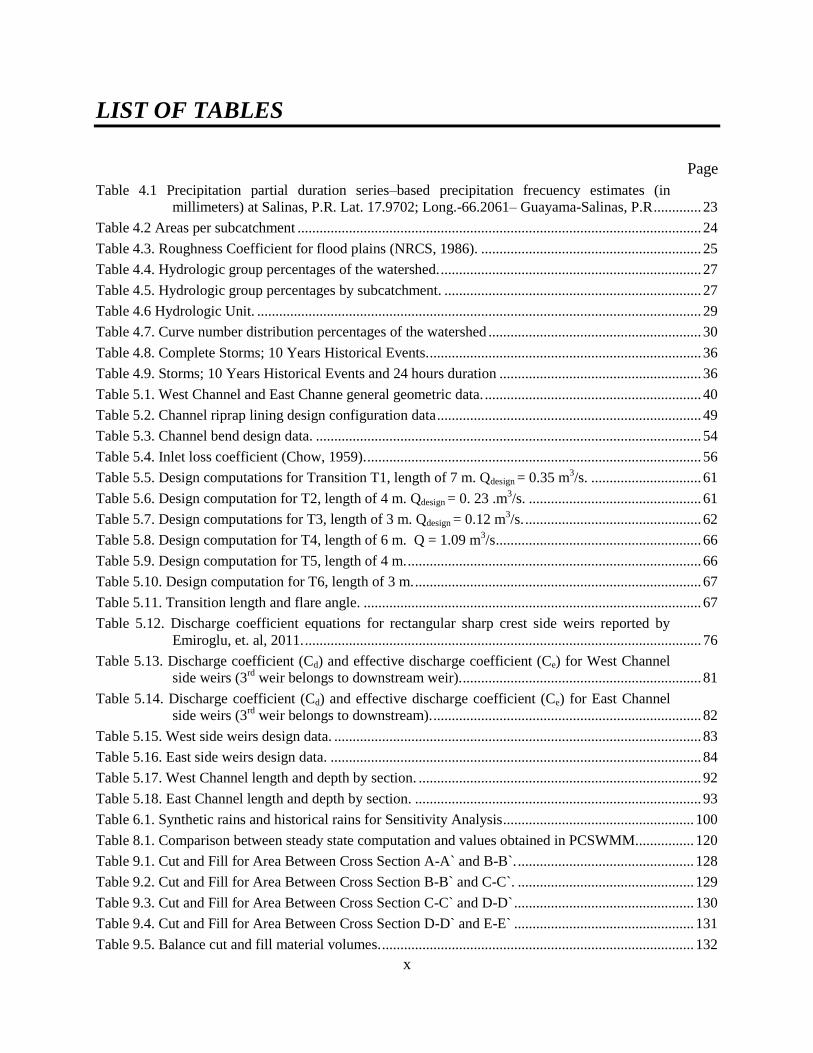
LIST OF TABLES
Page
Table 4.1 Precipitation partial duration series–based precipitation frecuency estimates (in
millimeters) at Salinas, P.R. Lat. 17.9702; Long.-66.2061– Guayama-Salinas, P.R ............. 23
Table 4.2 Areas per subcatchment .............................................................................................................. 24
Table 4.3. Roughness Coefficient for flood plains (NRCS, 1986). ............................................................ 25
Table 4.4. Hydrologic group percentages of the watershed. ....................................................................... 27
Table 4.5. Hydrologic group percentages by subcatchment. ...................................................................... 27
Table 4.6 Hydrologic Unit. ......................................................................................................................... 29
Table 4.7. Curve number distribution percentages of the watershed .......................................................... 30
Table 4.8. Complete Storms; 10 Years Historical Events. .......................................................................... 36
Table 4.9. Storms; 10 Years Historical Events and 24 hours duration ....................................................... 36
Table 5.1. West Channel and East Channe general geometric data. ........................................................... 40
Table 5.2. Channel riprap lining design configuration data ........................................................................ 49
Table 5.3. Channel bend design data. ......................................................................................................... 54
Table 5.4. Inlet loss coefficient (Chow, 1959). ........................................................................................... 56
Table 5.5. Design computations for Transition T1, length of 7 m. Qdesign = 0.35 m3/s. .............................. 61
Qdesign = 0. 23 .m3/s. ............................................... 61 Table 5.6. Design computation for T2, length of 4 m.
Table 5.7. Design computations for T3, length of 3 m. Qdesign = 0.12 m3/s. ................................................ 62
Table 5.8. Design computation for T4, length of 6 m. Q = 1.09 m3/s ........................................................ 66
Table 5.9. Design computation for T5, length of 4 m. ................................................................................ 66
Table 5.10. Design computation for T6, length of 3 m. .............................................................................. 67
Table 5.11. Transition length and flare angle. ............................................................................................ 67
Table 5.12. Discharge coefficient equations for rectangular sharp crest side weirs reported by
Emiroglu, et. al, 2011. ............................................................................................................ 76
Table 5.13. Discharge coefficient (Cd) and effective discharge coefficient (Ce) for West Channel
side weirs (3rd
weir belongs to downstream weir). ................................................................. 81
Table 5.14. Discharge coefficient (Cd) and effective discharge coefficient (Ce) for East Channel
side weirs (3rd
weir belongs to downstream). ......................................................................... 82
Table 5.15. West side weirs design data. .................................................................................................... 83
Table 5.16. East side weirs design data. ..................................................................................................... 84
Table 5.17. West Channel length and depth by section. ............................................................................. 92
Table 5.18. East Channel length and depth by section. .............................................................................. 93
Table 6.1. Synthetic rains and historical rains for Sensitivity Analysis .................................................... 100
Table 8.1. Comparison between steady state computation and values obtained in PCSWMM................ 120
Table 9.1. Cut and Fill for Area Between Cross Section A-A` and B-B`. ................................................ 128
Table 9.2. Cut and Fill for Area Between Cross Section B-B` and C-C`. ................................................ 129
Table 9.3. Cut and Fill for Area Between Cross Section C-C` and D-D` ................................................. 130
Table 9.4. Cut and Fill for Area Between Cross Section D-D` and E-E` ................................................. 131
Table 9.5. Balance cut and fill material volumes. ..................................................................................... 132

xi
Table 9.6. Grouted Riprap Lining Estimate Cost. ..................................................................................... 135
Table 9.7. Reinforced Concrete Lining Cost Estimate. Channel wall and bed width is 0.15 m. .............. 135
Table 9.8. Cost Estimate for Grouted Riprap Linning. ............................................................................. 136
Table 9.9. Cost Estimate adding the clearing, cut and fill of the A.O.I (optional). .................................. 137
Table A.1. Curve Number For hydrologic soil groups (NRCS, 1986). ...................................... 144

xii
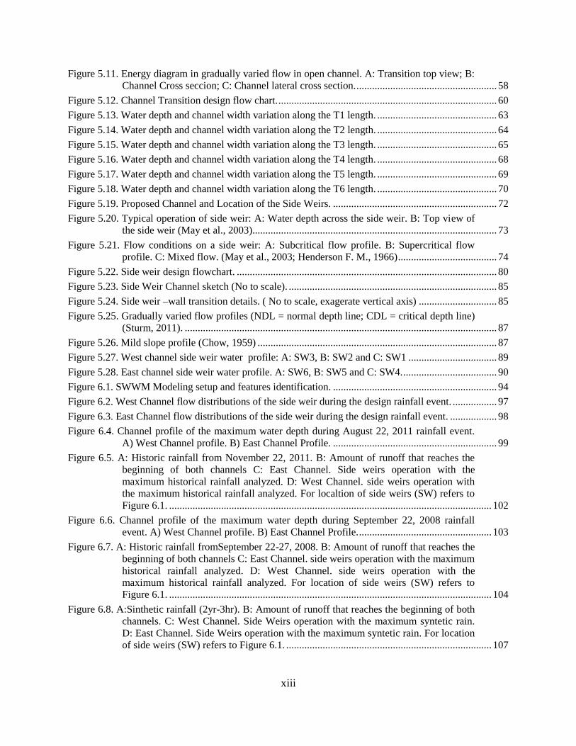
LIST OF FIGURES
Page
Figure 1.1. Location of Jobos Bay National Estuarine Research Reserve, JBNERRS delineated
areas shapefile from NERRS. .................................................................................................. 3
Figure 1.2. Location of the drainage channels. (Aereal image by 3001, Inc. 2007) ..................................... 3
Figure 1.3. Sequence of aereal photos showing the evolution of the project area during the last
decade. Project area shown in the orange box. Aereal Images by 3001 Inc., 2007 ................ 5
Figure 2.1. Jobos Bay National Estuarine Research Reserve (Zitello, Whitall, Dieppa,
Christensen, Monaco, and Rohman, 2008). ............................................................................. 8
Figure 2.2. Land use distribution in Central Aguirre watershed and percentage coverage (Zitello,
Whitall, Dieppa, Christensen, Monaco, & Rohman, 2008). .................................................... 8
Figure 2.3. A: Topographic measure points of the study area. B: Contour lines and elevation
modeling of the study area (msl). ............................................................................................. 9
Figure 2.4. Hydrogeology of the Jobos Bay watershed (Rodríguez, 2006). ............................................... 11
Figure 2.5. Hydrogeology cross section A-A’ from south to north bound of the Jobos Bay
Watershed (Rodríguez, 2006). ............................................................................................... 12
Figure 3.1. Illustration of the water balance variables and surface runoff computation. ............................ 16
Figure 3.2. Weir schematics: A: lateral view of the weir; B: Top view of the wier. .................................. 19
Figure 4.1. Deliniated watershed of AOI . .................................................................................................. 24
Figure 4.2. Representation of the hydrologic group. .................................................................................. 27
Figure 4.3. SCS map units. ......................................................................................................................... 29
Figure 4.4 Weighted curve number by watershed ...................................................................................... 30
Figure 4.5. Hyetograph of historical storm of September 22, 2008 showing the distribution of the
rain along 24 hours. ................................................................................................................ 31
Figure 4.6. Irrigation subareas for the pivot area at north of Jobos Bay (William C. O. et al.,
2012). ..................................................................................................................................... 32
Figure 4.7. PCSWMM maximum surface runoff by subcatchment. ........................................................... 34
Figure 5.1. General flowchart of the hydraulic Design. .............................................................................. 38
Figure 5.2. Channel Design Setup. ............................................................................................................. 40
Figure 5.3. Flow chart of the riprap design procedure (Anderson et al., 1970). ......................................... 44
Figure 5.4. Chart to determine the angle of repose of riprap in terms of the stone diameter chosen
and the shape (Anderson et al., 1970). ................................................................................... 46
Figure 5.5. Trapezoidal channel diagram. ................................................................................................... 47
Figure 5.6. Riprap channel design, not at scale. For dimension of b and B please see the Table 5.2 ......... 49
Figure 5.7. Superelevation profile. .............................................................................................................. 50
Figure 5.8. Cross section sketch of secondary flow characterstics in a channel bend (Blanckaert et
al., 2004). ............................................................................................................................... 51
Figure 5.9. A: Channel diagram. B: Dimensionless coefficient for shear stress caused by channel
bends calculation (Akan, 2006).............................................................................................. 53
Figure 5.10. Transition types (Federal Highway Administration, 2012). ................................................... 54
xiii
Figure 5.11. Energy diagram in gradually varied flow in open channel. A: Transition top view; B:
Channel Cross seccion; C: Channel lateral cross section. ...................................................... 58
Figure 5.12. Channel Transition design flow chart. .................................................................................... 60
Figure 5.13. Water depth and channel width variation along the T1 length. .............................................. 63
Figure 5.14. Water depth and channel width variation along the T2 length. .............................................. 64
Figure 5.15. Water depth and channel width variation along the T3 length. .............................................. 65
Figure 5.16. Water depth and channel width variation along the T4 length. .............................................. 68
Figure 5.17. Water depth and channel width variation along the T5 length. .............................................. 69
Figure 5.18. Water depth and channel width variation along the T6 length. .............................................. 70
Figure 5.19. Proposed Channel and Location of the Side Weirs. ............................................................... 72
Figure 5.20. Typical operation of side weir: A: Water depth across the side weir. B: Top view of
the side weir (May et al., 2003).............................................................................................. 73
Figure 5.21. Flow conditions on a side weir: A: Subcritical flow profile. B: Supercritical flow
profile. C: Mixed flow. (May et al., 2003; Henderson F. M., 1966) ...................................... 74
Figure 5.22. Side weir design flowchart. .................................................................................................... 80
Figure 5.23. Side Weir Channel sketch (No to scale). ................................................................................ 85
Figure 5.24. Side weir –wall transition details. ( No to scale, exagerate vertical axis) .............................. 85
Figure 5.25. Gradually varied flow profiles (NDL = normal depth line; CDL = critical depth line)
(Sturm, 2011). ........................................................................................................................ 87
Figure 5.26. Mild slope profile (Chow, 1959) ............................................................................................ 87
Figure 5.27. West channel side weir water profile: A: SW3, B: SW2 and C: SW1 .................................. 89
Figure 5.28. East channel side weir water profile. A: SW6, B: SW5 and C: SW4. .................................... 90
Figure 6.1. SWWM Modeling setup and features identification. ............................................................... 94
Figure 6.2. West Channel flow distributions of the side weir during the design rainfall event. ................. 97
Figure 6.3. East Channel flow distributions of the side weir during the design rainfall event. .................. 98
Figure 6.4. Channel profile of the maximum water depth during August 22, 2011 rainfall event.
A) West Channel profile. B) East Channel Profile. ............................................................... 99
Figure 6.5. A: Historic rainfall from November 22, 2011. B: Amount of runoff that reaches the
beginning of both channels C: East Channel. Side weirs operation with the
maximum historical rainfall analyzed. D: West Channel. side weirs operation with
the maximum historical rainfall analyzed. For localtion of side weirs (SW) refers to
Figure 6.1. ............................................................................................................................ 102
Figure 6.6. Channel profile of the maximum water depth during September 22, 2008 rainfall
event. A) West Channel profile. B) East Channel Profile. ................................................... 103
Figure 6.7. A: Historic rainfall fromSeptember 22-27, 2008. B: Amount of runoff that reaches the
beginning of both channels C: East Channel. side weirs operation with the maximum
historical rainfall analyzed. D: West Channel. side weirs operation with the
maximum historical rainfall analyzed. For location of side weirs (SW) refers to
Figure 6.1. ............................................................................................................................ 104
Figure 6.8. A:Sinthetic rainfall (2yr-3hr). B: Amount of runoff that reaches the beginning of both
channels. C: West Channel. Side Weirs operation with the maximum syntetic rain.
D: East Channel. Side Weirs operation with the maximum syntetic rain. For location
of side weirs (SW) refers to Figure 6.1. ............................................................................... 107
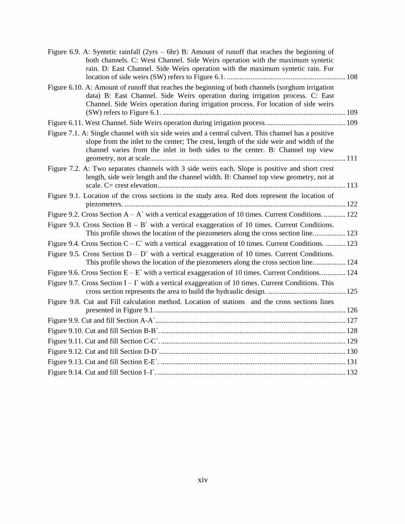
xiv
Figure 6.9. A: Syntetic rainfall (2yrs – 6hr) B: Amount of runoff that reaches the beginning of
both channels. C: West Channel. Side Weirs operation with the maximum syntetic
rain. D: East Channel. Side Weirs operation with the maximum syntetic rain. For
location of side weirs (SW) refers to Figure 6.1. ................................................................. 108
Figure 6.10. A: Amount of runoff that reaches the beginning of both channels (sorghum irrigation
data) B: East Channel. Side Weirs operation during irrigation process. C: East
Channel. Side Weirs operation during irrigation process. For location of side weirs
(SW) refers to Figure 6.1. .................................................................................................... 109
Figure 6.11. West Channel. Side Weirs operation during irrigation process. ........................................... 109
Figure 7.1. A: Single channel with six side weirs and a central culvert. This channel has a positive
slope from the inlet to the center; The crest, length of the side weir and width of the
channel varies from the inlet in both sides to the center. B: Channel top view
geometry, not at scale. .......................................................................................................... 111
Figure 7.2. A: Two separates channels with 3 side weirs each. Slope is positive and short crest
length, side weir length and the channel width. B: Channel top view geometry, not at
scale. C= crest elevation. ...................................................................................................... 113
Figure 9.1. Location of the cross sections in the study area. Red dots represent the location of
piezometers. ......................................................................................................................... 122
Figure 9.2. Cross Section A – A` with a vertical exaggeration of 10 times. Current Conditions. ............ 122
Figure 9.3. Cross Section B – B` with a vertical exaggeration of 10 times. Current Conditions.
This profile shows the location of the piezometers along the cross section line. ................. 123
Figure 9.4. Cross Section C – C` with a vertical exaggeration of 10 times. Current Conditions. ........... 123
Figure 9.5. Cross Section D – D` with a vertical exaggeration of 10 times. Current Conditions.
This profile shows the location of the piezometers along the cross section line.. ................ 124
Figure 9.6. Cross Section E – E` with a vertical exaggeration of 10 times. Current Conditions. ............. 124
Figure 9.7. Cross Section I – I` with a vertical exaggeration of 10 times. Current Conditions. This
cross section represents the area to build the hydraulic design. ........................................... 125
Figure 9.8. Cut and Fill calculation method. Location of stations and the cross sections lines
presented in Figure 9.1. ........................................................................................................ 126
Figure 9.9. Cut and fill Section A-A`. ....................................................................................................... 127
Figure 9.10. Cut and fill Section B-B`. ..................................................................................................... 128
Figure 9.11. Cut and fill Section C-C`. ..................................................................................................... 129
Figure 9.12. Cut and fill Section D-D`...................................................................................................... 130
Figure 9.13. Cut and fill Section E-E`. ..................................................................................................... 131
Figure 9.14. Cut and fill Section I–I`. ....................................................................................................... 132
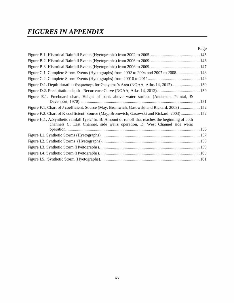
xv
FIGURES IN APPENDIX
Page
Figure B.1. Historical Rainfall Events (Hyetographs) from 2002 to 2005. .............................................. 145
Figure B.2. Historical Rainfall Events (Hyetographs) from 2006 to 2009. .............................................. 146
Figure B.3. Historical Rainfall Events (Hyetographs) from 2006 to 2009. .............................................. 147
Figure C.1. Complete Storm Events (Hyetographs) from 2002 to 2004 and 2007 to 2008. ..................... 148
Figure C.2. Complete Storm Events (Hyetographs) from 20010 to 2011................................................. 149
Figure D.1. Depth-duration-frequencys for Guayama’s Area (NOAA, Atlas 14, 2012). ......................... 150
Figure D.2. Precipitation depth - Recurrence Curve (NOAA, Atlas 14, 2012). ....................................... 150
Figure E.1. Freeboard chart. Height of bank above water surface (Anderson, Paintal, &
Davenport, 1970). ................................................................................................................ 151
Figure F.1. Chart of J coefficient. Source (May, Bromwich, Gasowski and Rickard, 2003) ................... 152
Figure F.2. Chart of K coefficient. Source (May, Bromwich, Gasowski and Rickard, 2003) .................. 152
Figure H.1. A:Synthetic rainfall.1yr-24hr. B: Amount of runoff that reaches the beginning of both
channels C: East Channel. side weirs operation. D: West Channel side weirs
operation............................................................................................................................... 156
Figure I.1. Synthetic Storms (Hyetographs). ............................................................................................ 157
Figure I.2. Synthetic Storms (Hyetographs). ........................................................................................... 158
Figure I.3. Synthetic Storm (Hyetographs). .............................................................................................. 159
Figure I.4. Synthetic Storm (Hyetographs). .............................................................................................. 160
Figure I.5. Synthetic Storm (Hyetographs). ............................................................................................. 161

xvi
LIST OF ACRONYMS
AOI Area of Interest
ASCE America Society of Civil Engineers
CDL Critical Depth Line
cm Centimeter
CN Runoff Curve Number
CSS Critical Shear Stress
CY Cubic Yard
DDF Depth-Duration Frecuency Curve
DEM Digital Elevation Model
EGL Energy Grade Line
EPA Environmental Protection Agency
ESRI Economic and Socila Research Institute
FHWA Federal Highway highway Administration
GIS Geographic Information System
HGL Hidraulic Grade Line
hr Hours
JBNERR Jobos Bay National Estuarine Research Reserve
MGD Million Gallons Per day
msl Mean sea level
MSS Maximum Shear Stress
NCDC National Climatic Data Center
NCHRP National Cooperative Highway Research Program
NDL Normal Depth Line
NERRS National Estuarine Research Reserve System
NOAA National Oceanic and Atmospheric Admin
NRCS Natural Resources Conservation Service
PCSWMM PC Storm Water Management Model (SWMM)
PRASA P.R. Aqueduct and Sewer. Authority
PRLA Puerto Rico Land Authority
SCS Soil Conservation Service
SI International System ( Metric System)
USCS United States Customary System
USDA U.S. Department of Agriculture
USGS U.S. Geological Survey
VBA Visual Basics for Aplications
WEF Water Environmental Federation
WSS NRCS - Web Soil Survey
1
CHAPTER 1 INTRODUCTION
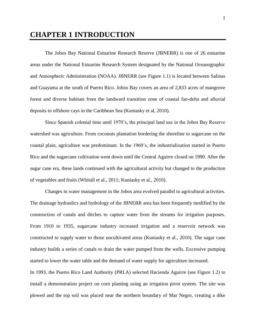
The Jobos Bay National Estuarine Research Reserve (JBNERR) is one of 26 estuarine
areas under the National Estuarine Research System designated by the National Oceanographic
and Atmospheric Administration (NOAA). JBNERR (see Figure 1.1) is located between Salinas
and Guayama at the south of Puerto Rico. Jobos Bay covers an area of 2,833 acres of mangrove
forest and diverse habitats from the landward transition zone of coastal fan-delta and alluvial
deposits to offshore cays in the Caribbean Sea (Kuniasky et al, 2010).
Since Spanish colonial time until 1970’s, the principal land use in the Jobos Bay Reserve
watershed was agriculture. From coconuts plantation bordering the shoreline to sugarcane on the
coastal plain, agriculture was predominant. In the 1960’s, the industrialization started in Puerto
Rico and the sugarcane cultivation went down until the Central Aguirre closed on 1990. After the
sugar cane era, these lands continued with the agricultural activity but changed to the production
of vegetables and fruits (Whitall et al., 2011; Kuniasky et al., 2010).
Changes in water management in the Jobos area evolved parallel to agricultural activities.
The drainage hydraulics and hydrology of the JBNERR area has been frequently modified by the
construction of canals and ditches to capture water from the streams for irrigation purposes.
From 1910 to 1935, sugarcane industry increased irrigation and a reservoir network was
constructed to supply water to those uncultivated areas (Kuniasky et al., 2010). The sugar cane
industry builds a series of canals to drain the water pumped from the wells. Excessive pumping
started to lower the water table and the demand of water supply for agriculture increased.
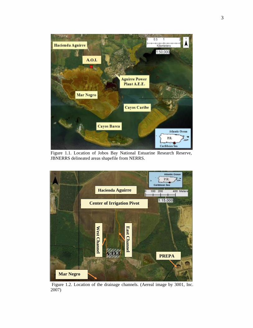
In 1993, the Puerto Rico Land Authority (PRLA) selected Hacienda Aguirre (see Figure 1.2) to
install a demonstration project on corn planting using an irrigation pivot system. The site was
plowed and the top soil was placed near the northern boundary of Mar Negro, creating a dike

2
which was used as roadway. This dike altered of the flow pattern in the zone. Due to this action,
six of seven abandoned ditches were cleaned and excavated. These ditches (two of them are in
the area of interest of this project) drains from north to south, directly into the mangrove forest
(Gregory L. Morris and Associates, 2000).
It is believed that intensive agricultural activities north of the reserve caused a negative
impact on mangroves. In 1993, as part of the demonstration project, PRLA cleaned a series of
drainage channels to drain irrigation water excess direct to the mangrove forest (Gregory L.
Morris and Associates, 2000). Figure 1.2 shows two of the channels that belong to the area of
interest. The east channel starts at the center of the irrigation pivot and extends to the south
toward the mangrove forest. This channel used to discharge fresh water from pumps, however,
nowadays fresh water comes from leakage through the pumps. The west channel collects the
water excess from the west side of the center pivot irrigation.
Preliminary studies reported that pesticides, fertilizers and chicken manure applied in agricultural
fields were being transported and impacted the near-shore water and air in the estuary (Dieppa et
al., 2008; Whitall et al., 2011). Both channels in Figure 1.2 were used to transport runoff and
irrigation water directly into the mangrove area.
1.1 PROBLEM STATEMENT
3
Figure 1.1. Location of Jobos Bay National Estuarine Research Reserve,
JBNERRS delineated areas shapefile from NERRS.
A.O.I.
Figure 1.2. Location of the drainage channels. (Aereal image by 3001, Inc.
2007)
Hacienda Aguirre Hacienda Aguirre
Center of Irrigation Pivot
Mar Negro
PREPA
East C
ha
nn
el
West C
ha
nn
el

4
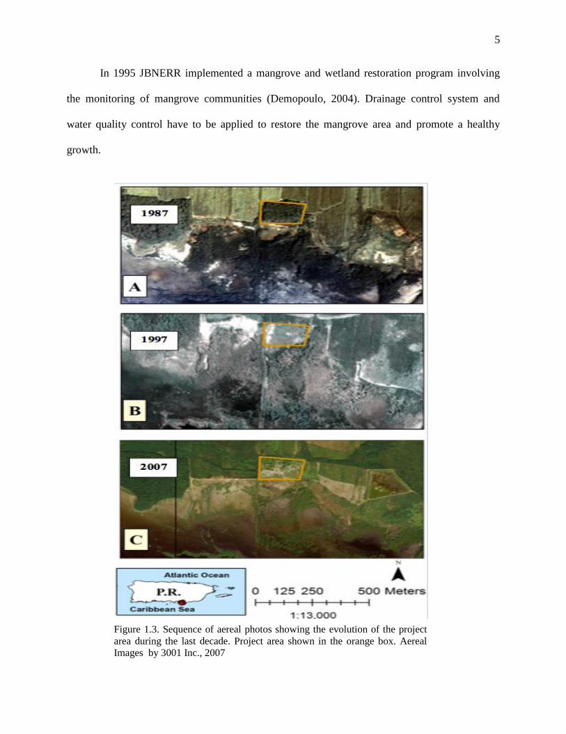
Nevertheless, the northern area of the Jobos Bay Reserve has been used for agricultural
activities since the Spanish colonial times. Figure 1.3.A shows the study area in 1987. At this
time agriculture was present under the sugar mill Central Aguirre until 1990 when this industry
closed operations. In 1993, the center pivot irrigator system was introduced near the mangrove
forest. Figure 1.3.B demonstrates that by 1997 the mangrove cover was residing. This irrigation
method was operational until late 2009 when the PRLA decided to stop operations to upgrade the
system. However, at current time, it remains non-operational.
In 1998, the Hurricane Georges affected the area causing great damage to the mangrove
forest. The overall impact of hurricane Georges on Jobos Bay mangroves is not known with
precision; however, hurricanes generally set back succession and reduce mangrove areas
(Demopoulos, 2004). Figure 1.3.C shows the situation of the mangroves forest in 2007 which is
similar to current conditions.
The mangrove mortality can be induced by anthropogenic activities such as deforestation,
domestic sewage inputs to mangrove lagoons, change of hydrology by the constructions and
agricultural practices at nearby locations (Román Guzmán, 2010). The mortality may be
increased by natural factors such as hurricanes, storms, tsunamis, droughts, hydrologic changes,
erosion and subsidence, hypersalinity, and pollution. Any of these factors can contribute to the
mangrove mortality on the Jobos area, especially those which involve agricultural activities,
change of hydrology and the natural factors such as the ones already observed in that area.
However, the affected mangrove stand is over 30 years old and its proximity to farms bordering
the JBNERR may indicate that the hydrology has changed as a result of changes in irrigation
practices, water use, and rainfall (Kuniasky et al., 2010).
5
In 1995 JBNERR implemented a mangrove and wetland restoration program involving
the monitoring of mangrove communities (Demopoulo, 2004). Drainage control system and
water quality control have to be applied to restore the mangrove area and promote a healthy
growth.
Figure 1.3. Sequence of aereal photos showing the evolution of the project
area during the last decade. Project area shown in the orange box. Aereal
Images by 3001 Inc., 2007

6
The purpose of this project is the design of an innovative overland flow water distribution
system using lateral weirs to control surface runoff, reduce surface erosion and improve the
quality of runoff waters discharging into the Jobos Bay mangrove area. The project will be
focused on hydrologic and hydraulic design conditions according to the runoff and to the
irrigation flow discharging into the project area. A cost analysis of the channels system, land
movement, labor, materials and equipment is provided to complete the design.
1.2 SCOPE AND OBJECTIVE OF THE STUDY

7
CHAPTER 2 STUDY AREA DESCRIPTION
The JBNERR is the second largest estuary in Puerto Rico and it is part of the National
Estuarine Research Reserve System (NERRS) of NOAA. Jobos bay is located on the southeast
coast of the island between the municipalities of Salinas and Guayama. The contributing
watershed of this bay has an area of about 137 km2 with a population of about 32,000 persons
and a variety of land uses, predominantly agriculture (Whitall et. al, 2011). The Jobos Bay
Reserve has a total surface area of 25 km2 (Dieppa et al., 2008) and it is composed by areas
knows as: Mar Negro, Hacienda Aguirre, Cayos Barca, and Cayos Caribe (see orange shaded
areas in Figure 1.1). The area of interest (A.O.I.) for this project is a parcel located at the
boundary between Mar Negro and Hacienda Aguirre (see Figure 1.2). Hacienda Aguirre shows a
circular area with the pivot irrigation system.
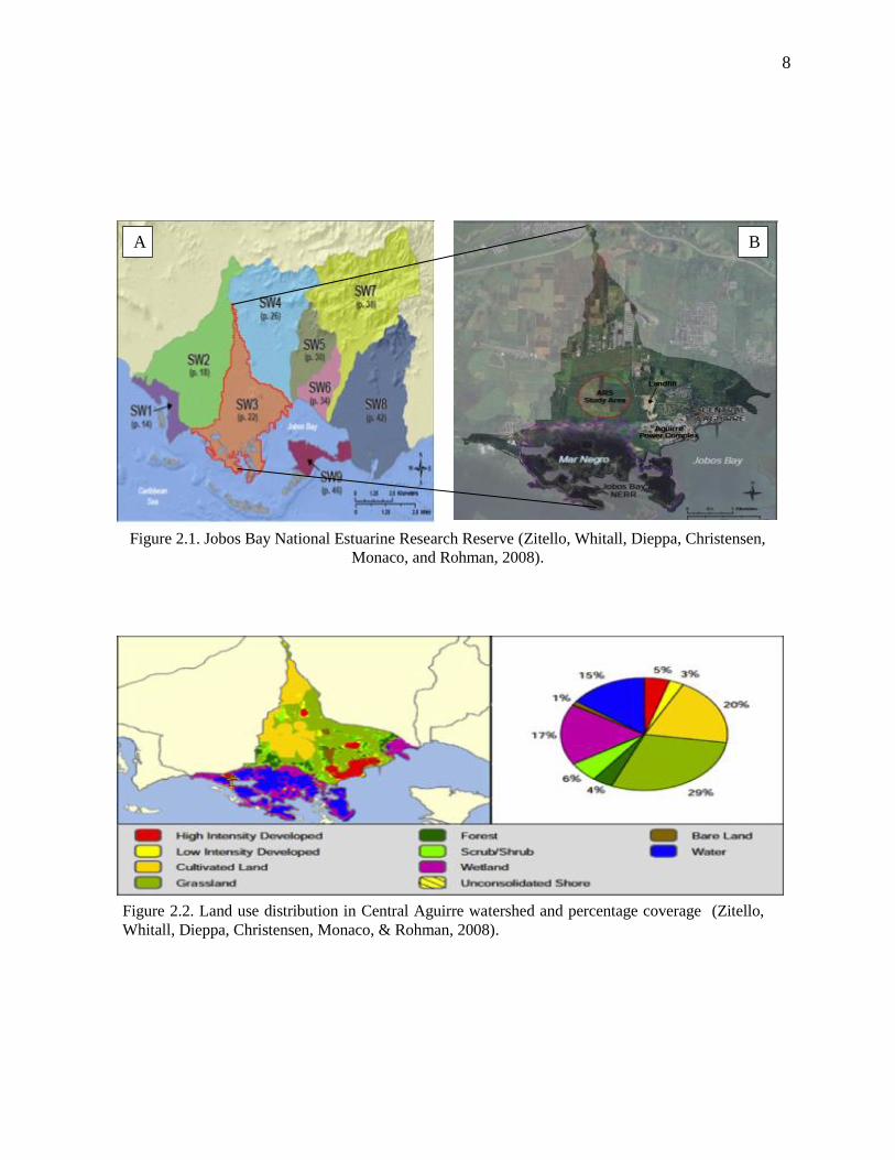
The JBNERR watershed could be subdivided into nine subwatersheds (Figure 2.1.A) and the
project area belongs to SW3 (Figure 2.1.B) with an area of 16.5 km2 which extends from highway PR-
52 to Jobos Bay coastline (Mar Negro wetland system). Similar to other Jobos Bay subwatersheds, the
SW3 does not have a defined stream channel and the surface runoff discharges in several places of the
bay depending on the topography.
This watershed has a diversity of land uses (see Figure 2.2) including industrial;
residential development (which includes a population of about 2,652 residents, Census 2000),
agriculture, wetlands areas, and forest areas. The dominant feature in the watershed is Mar
Negro’s mangrove forests and associated tidal waterways and mud flats (Zitello et al., 2008).
2.1 Location and Physiographic Region
8
B A
Figure 2.1. Jobos Bay National Estuarine Research Reserve (Zitello, Whitall, Dieppa, Christensen,
Monaco, and Rohman, 2008).
Figure 2.2. Land use distribution in Central Aguirre watershed and percentage coverage (Zitello,
Whitall, Dieppa, Christensen, Monaco, & Rohman, 2008).
9
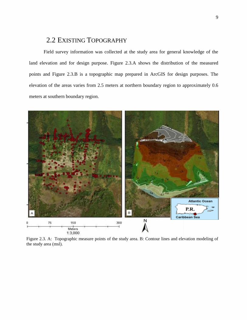
Field survey information was collected at the study area for general knowledge of the
land elevation and for design purpose. Figure 2.3.A shows the distribution of the measured
points and Figure 2.3.B is a topographic map prepared in ArcGIS for design purposes. The
elevation of the areas varies from 2.5 meters at northern boundary region to approximately 0.6
meters at southern boundary region.
2.2 EXISTING TOPOGRAPHY
Figure 2.3. A: Topographic measure points of the study area. B: Contour lines and elevation modeling of
the study area (msl).
10
The watershed of Central Aguirre, as part of Jobos Bay, it is primarily comprised of the
low relief South Coastal Plain of Puerto Rico. A natural mountain range (La Coordillera Central
and La Sierra de Cayey) at the north of Jobos Bay watershed, protects the zone from moisture-
laden northeast trade winds, causing a zone of low precipitation in the study area (Whitall, et al.,
2011). Jobos Bay receives a mean precipitation of approximately 15.4 cm/yr (National Weather
Service, Weather Forecast Office, 2009). During the period between 1999 to 2008 the mean
precipitation was 99.6 cm at the Aguirre Gauge station, within the watershed boundaries. The
wettest months are September and October with 167 mm and the driest month with 20 mm of
rain is January (National Climatic Data Center (NCDC), 2010). The mean annual temperature
between 1999 and 2008 was 26º C with a maximum of 27.5º C in August and a minimum of
24.3º C in January (NCDC, 2010).
The evapotranspiration of the area is around 25.59 cm/yr and it usually decreases as the water
table level reaches a depth of aproximately 2 meters from the surface (Rodríguez, 2006). This
aquifer does not have great importance in the area but most of the domestic wells in the zone
take their supply from the upper zone of this aquifer. The Puerto Rico Aqueduct and Sewer
Authority (PRASA) and the water used for agriculture are collected from the unconfined aquifer
that can be found at the bottom of the alluvial formation.
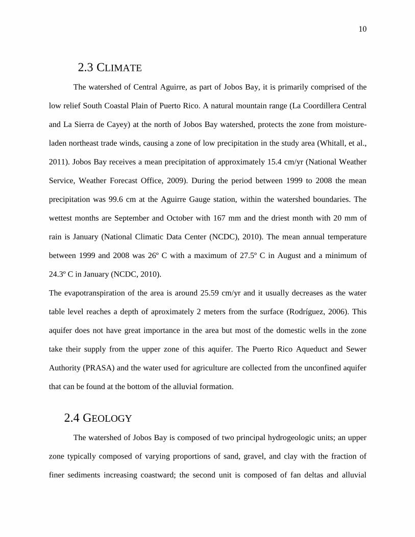
The watershed of Jobos Bay is composed of two principal hydrogeologic units; an upper
zone typically composed of varying proportions of sand, gravel, and clay with the fraction of
finer sediments increasing coastward; the second unit is composed of fan deltas and alluvial
2.3 CLIMATE
2.4 GEOLOGY
11
deposits (Rodríguez, 2006). The alluvial deposits involve the coastal plain of the area and swamp
deposits (unconsolidated clay, silt and organic matter) on the southern boundary of the coastal
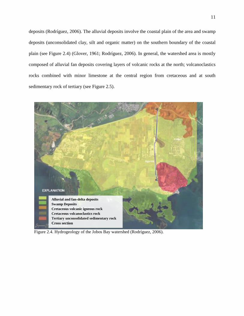
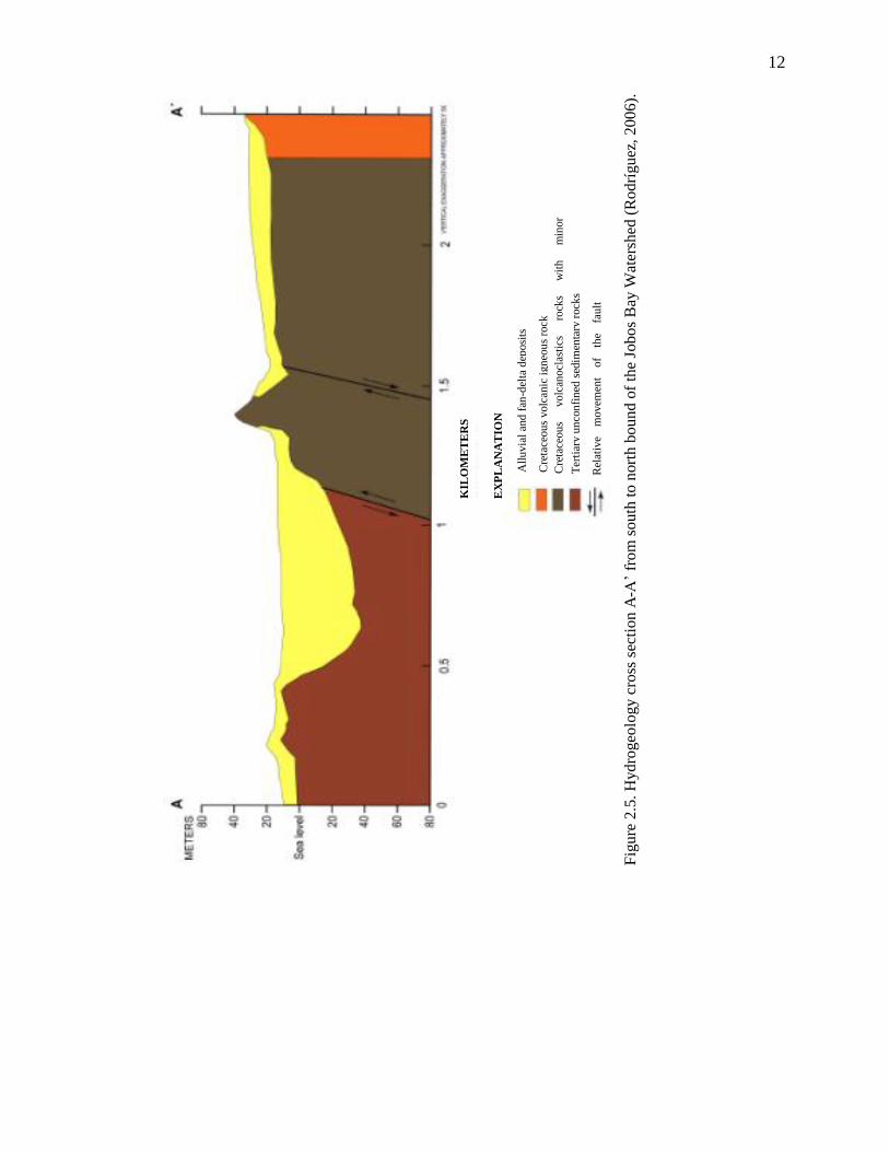
plain (see Figure 2.4) (Glover, 1961; Rodríguez, 2006). In general, the watershed area is mostly
composed of alluvial fan deposits covering layers of volcanic rocks at the north; volcanoclastics
rocks combined with minor limestone at the central region from cretaceous and at south
sedimentary rock of tertiary (see Figure 2.5).
Figure 2.4. Hydrogeology of the Jobos Bay watershed (Rodríguez, 2006).
Alluvial and fan-delta deposits
Swamp Deposits
Cretaceous volcanic igneous rock
Cretaceous volcanoclastics rock
Tertiary unconsolidated sedimentary rock
Cross section
12
Fig
ure
2.5
. H
ydro
geo
logy c
ross
sec
tion
A-A
’ fr
om
south
to n
ort
h b
ound
of
the
Job
os
Bay
Wat
ersh
ed (
Ro
drí
gu
ez,
20
06
).
Rel
ativ
e m
ovem
ent
of
the
fau
lt
Ter
tiar
y u
nco
nfi
ned
sed
imen
tary
rock
s
Cre
tace
ou
s volc
anocl
asti
cs
rock
s w
ith
m
inor
Cre
tace
ou
s volc
anic
ign
eou
s ro
ck
All
uvia
l an
d f
an-d
elta
dep
osi
ts
EX
PL
AN
AT
ION
KIL
OM
ET
ER
S
13
These alluvial deposits constitute the Salinas Alluvial Fan Aquifer, which extends from
Nigua river in Salinas to Guamani river in Guayama. This aquifer forms part of the Santa Isabel
– Patillas Region aquifer system. This aquifer unit covers the coastline area extending from one
(1) mile (at Bahía de Jobos) to four (4) mile (in the Salinas fan delta) inland (Quiñones-Aponte,
et al., 1996). One of the hydrogeological characteristis of this aquifer is the specific yield, is of
approximately 25 % (Quiñones-Aponte et al., 1996). That specific yield is a representation of the
unconfined conditions in the aquifer`s upper zone. The unconfined conditions varies as it
approaches to the coast by a fine-grains formation that acts as semiconfined condition
(Rodríguez, 2006). The storage coefficient of this aquifer was found to be around 0.0003 and the
hydraulic conductivity of the alluvial deposits were in a range from 8 m/d near to the Cordillera
Cental and 30 m/d close to the Salinas town and the coast.
Since late 1800`s until 1990 when the sugar cane era ended, the Hacienda Aguirre used
furrow irrigation. In 1994, a pivot drip systems and center-pivot sprinkler irrigation were
installed using groundwater wells. This new technology replaced the traditional flooding
irrigation practices (Dieppa et al., 2008). Changes in irrigation methods and the combination of
increased groundwater extraction, which reached up to 11.4 MGD in 2002 (Kuniasky et al.,
2010) contributed to lower groundwater levels and possibly shorten the aquifer recharge time.
This has increased the risk for salt water intrusion into the aquifer (Kuniasky et al., 2010). The
effect of this process on the mangrove ecosystem has not been documented; however, pivot
irrigation is not used nowadays. In some farms, drip irrigation has been implemented.
1.1 AGRICULTURAL ACTIVITIES

14
CHAPTER 3 MODEL DESCRIPTION
Runoff in the watershed of Jobos Bay area was simulated using PC Storm Water
Management Model (PCSWMM1) based upon the Environmental Protection Agency (EPA)
model SWMM52
and including geographic information system (GIS) data formats. This
modeling software simulates the surface runoff response of a given catchment to preloaded
precipitation data by representing the subcatchments as an interconnected system of hydrologic
and hydraulic components. SWMM contains a series of capabilities and limitations for the Jobos
Bay project:
The software PCSWMM allows inputs from Economic and Social Research Institute
(ESRI) format shapefiles, images, and digital elevation models (DEM). This interaction
let the user to use the remote sensing knowledge to create a scenario that fits more with
the existent conditions. On this project, these features allow to recreate a possible future
scenario of the proposed hydrologic conditions.
The model was used to analyze historical rain fall data from 2002 to 2011. These periods
contains only the maximum accumulative rain in 24 hours events for each year.
Maximum annual 24-hr duration events from 2002 to 2011 were simulated with SWMM.
Rainfall data was obtained from the JBNERR weather station of the main office which is
located approximately 2.5 km east of the project area. The effect of the distance is not
1 PCSWMM is a marketed software develop by Computational Hydraulics International (CHI).
2 Storm Water Management Model (SWMM)
3.1 RUNOFF AND HYDRAULIC SIMULATION

15
significant because most 24 hours events are associated with tropical storms covering the
entire watershed.
The model simulates the infiltration. The user could select the soil conservation service
Curve Number, Horton or Green-Ampt models. Also the software let change from one
method to another, but the data required by each method have to be available.
The software allows defining a large variety of open channels geometries. It creates a
connection of the rainfall runoff simulation with the hydraulics elements and is capable to
simulate the water behavior on the system.
Channel transitions (contraction or expansion) cannot be modeled on SWMM. There are
no features which identify the transition elements. The lengths of the transitions are not
considered by the model software.
Channel bends analyses are not considered by SWMM. The superelevation effects in the
water surface of the channel bend is not taken in consideration.
This project consist in two differents modeling parts, the hydrology, which determines
the surfaces runoff for the given subwatershed and the design of open channels with different
features. The mathematical basis of the hydrological and hydraulic designs will be summarized
in two sections following the EPA SWMM User Manual 3(James et al., 2011).
3 PCSWMM use the EPA SWMM User Manual.
3.2 CONCEPTUAL MODEL.
16
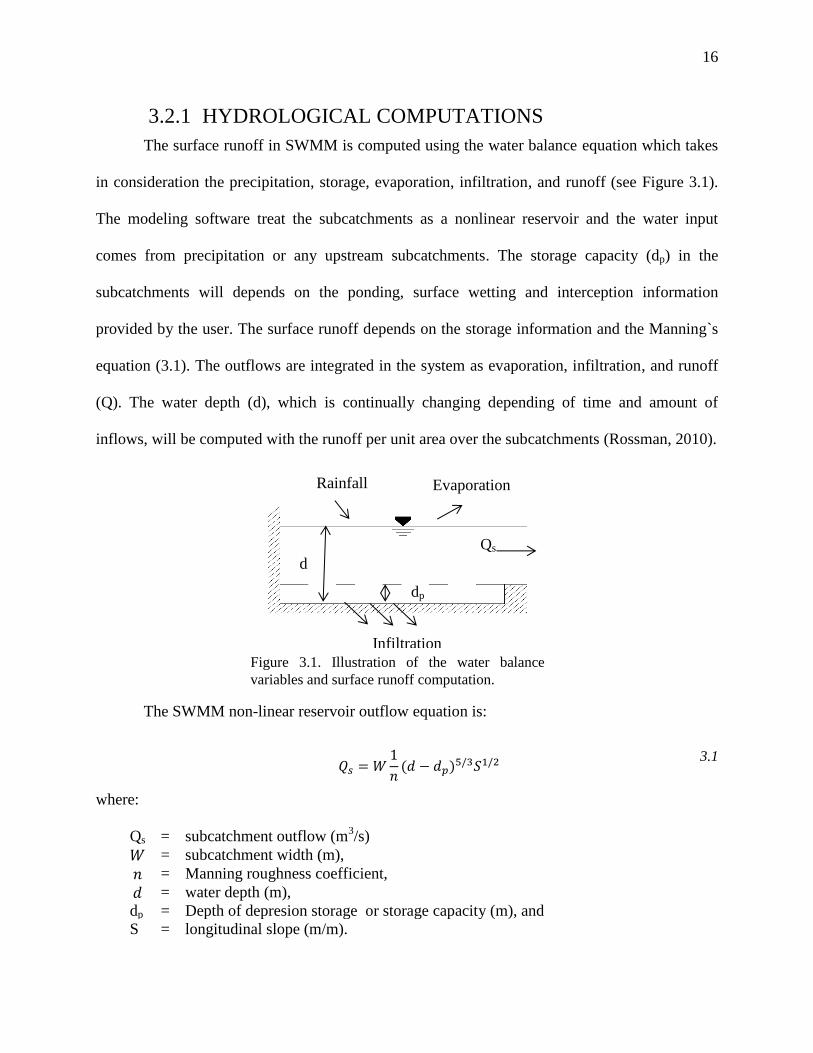
The surface runoff in SWMM is computed using the water balance equation which takes
in consideration the precipitation, storage, evaporation, infiltration, and runoff (see Figure 3.1).
The modeling software treat the subcatchments as a nonlinear reservoir and the water input
comes from precipitation or any upstream subcatchments. The storage capacity (dp) in the
subcatchments will depends on the ponding, surface wetting and interception information
provided by the user. The surface runoff depends on the storage information and the Manning`s
equation (3.1). The outflows are integrated in the system as evaporation, infiltration, and runoff
(Q). The water depth (d), which is continually changing depending of time and amount of
inflows, will be computed with the runoff per unit area over the subcatchments (Rossman, 2010).
The SWMM non-linear reservoir outflow equation is:
3.1
where:
Qs = subcatchment outflow (m3/s)
= subcatchment width (m),
= Manning roughness coefficient,
= water depth (m),
dp = Depth of depresion storage or storage capacity (m), and
S = longitudinal slope (m/m).
3.2.1 HYDROLOGICAL COMPUTATIONS
Figure 3.1. Illustration of the water balance
variables and surface runoff computation.
Qs
Rainfall Evaporation
Infiltration
d
dp
17
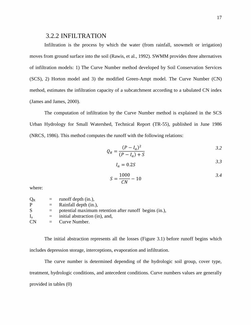
Infiltration is the process by which the water (from rainfall, snowmelt or irrigation)
moves from ground surface into the soil (Rawis, et al., 1992). SWMM provides three alternatives
of infiltration models: 1) The Curve Number method developed by Soil Conservation Services
(SCS), 2) Horton model and 3) the modified Green-Ampt model. The Curve Number (CN)
method, estimates the infiltration capacity of a subcatchment according to a tabulated CN index
(James and James, 2000).
The computation of infiltration by the Curve Number method is explained in the SCS
Urban Hydrology for Small Watershed, Technical Report (TR-55), published in June 1986
(NRCS, 1986). This method computes the runoff with the following relations:
3.2
3.3
3.4
where:
QR = runoff depth (in.),
P = Rainfall depth (in.),
S = potential maximum retention after runoff begins (in.),
Ia = initial abstraction (in), and,
CN = Curve Number.
The initial abstraction represents all the losses (Figure 3.1) before runoff begins which
includes depression storage, interceptions, evaporation and infiltration.
The curve number is determined depending of the hydrologic soil group, cover type,
treatment, hydrologic conditions, and antecedent conditions. Curve numbers values are generally
provided in tables (0)
3.2.2 INFILTRATION
18
The hydraulics computations will depend on the flows generated by the hydrologic
model. In general, SWMM represents the hydraulic system by different elements such as
conduits, nodes (junction, outfall, and flow divider nodes), storage units, pumps, flow regulators
and weirs. Some of these elements are used to model the hydraulic system proposed in this
project.
A conduit in the current project represents the open channel that moves the water from
SWMM node to another. Nodes are elements which links conduits. These elements are able to
represent confluence of natural surface channels and they can receive external inflows into the
channel system.
The conduits, in SWMM, can be represented in all geometric shapes. The user has the
option to draw transects of the channel or cross section. For this project, the trapezoidal
geometry was used for open channel simulation. This modeling software use the Manning
equation to express the relation between flow rate, channel bottom slope, cross sectional area,
and hydraulic radius. The principal input parameters for conduits are:
1) name of the inlet and outlet nodes,
2) offset height or elevation above the inlet and outlet node inverts,
3) conduit length
4) Manning’s roughness coefficient,
5) cross sectional geometry,
6) entrance/exit losses coefficients (optional), and
7) presence of a flap gate to prevent reverse flow (optional).
A channel transition, according to Chow, 1959, is a structure designed to change the
geometric shape or cross sectional area of the flow. A channel transition should avoid excessive
energy losses and eliminate cross waves and turbulence in order to provide safety to channel
walls. There are several types of transitions (that will be discussed on Chapter 5), and Chow
3.2.3 HYDRAULICS COMPUTATIONS
19
(1959) recommends a coefficient of inlet losses for each of those transitions. SWMM do not
have a particular element to analize the transition areas but, the conduits contain a section to
include the loss coefficient value at the entrance or at the outlet of each of them.
Side or lateral weirs are part of the flow regulator section in the SWMM user manual.
The manual describes the flow regulators as structures used to control or divert flows within a
conveyance system. Side weirs are represented in SWMM as a link connecting two nodes, where
the weir is placed upstream of the node. The principal inputs for side weirs are:
name of its inlet and outlet node,
shape and geometry,
crest height or elevation above the inlet node invert, and
discharge coefficient.
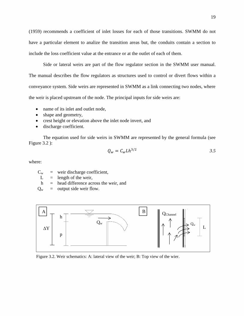
The equation used for side weirs in SWMM are represented by the general formula (see
Figure 3.2 ):
3.5
where:
Cw = weir discharge coefficient,
L = length of the weir,
h = head difference across the weir, and
Qw = output side weir flow.
3.2.4 FLOW ROUTING METHODS Figure 3.2. Weir schematics: A: lateral view of the weir; B: Top view of the wier.
h
∆Y
p
L
B
Qw
A
Qw
QChannel
20
Once the setup of the channel geometry is completed, SWMM can develop routing
calculations using the conservation of mass and momentum equations for gradually varied flow.
This software includes three different methods to solve previously mentioned equations; steady
flow, kinematic wave routing and dynamic wave routing.
The steady flow routing method assumes that flow is uniform and steady. This routing
method uses the inflow hydrographs at the channel upstream end to the downstream end without
delay or change of shape. This method assumes that the channel longitudinal slope is equal to the
friction slope of the channel.
The kinematic wave routing solves the continuity equation (3.6) and the simplified
version of the momentum equation (3.7) for each reach of the channel. The only requirement for
this method is that the slope of the water surface must be equal to the bottom slope of the
channel. This method uses the discharge corresponding to normal depth as the maximum flow
conveyed by the channel. Any amount of water that exceeds this value is considered lost from
the system or ponded. This method cannot calculate the backwater effect, entrance/exits losses,
or flow reversal.
Dynamic wave routing computes the complete one-dimensional Saint Venant flow
equations, obtaining more accurate results. This method solves the unsteady momentum and
continuity equations for each channel reach and computes the continuity equation in each node.
This method can compute the backwater effect, entrance/exits losses, and flow reversal because
it couples together the solution value of the water level from the channel conduits and the level at
the nodes. The requirement of this method is to use smaller time step, usually minutes or less
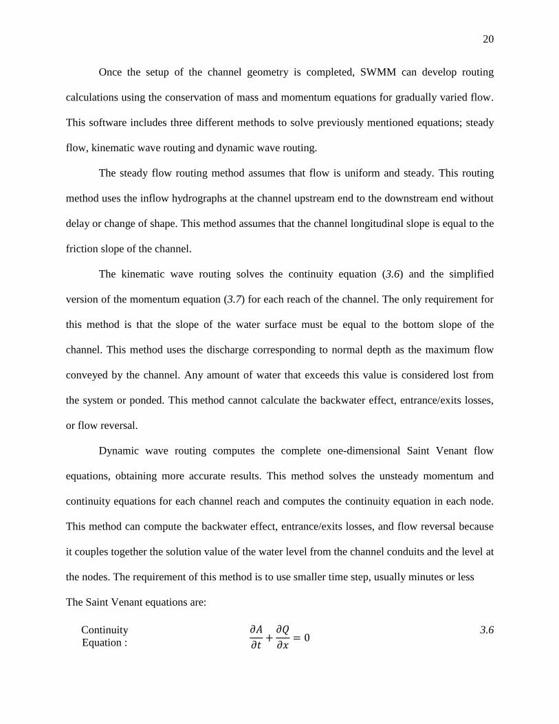
The Saint Venant equations are:
Continuity
Equation :
3.6

21
Dynamic
Equation:
3.7
Kinematic
Equation:
3.8
Steady State
Equation:
3.9
where:
A = cross-sectional area (m2),
t = mime (min),
Q = flow rate (m3/s),
H = hydraulic head of the water in the channel (m),
= friction slope = Q2n
2/(A
2R
4/3),
S0 = longitudinal slope (m/m),
= local energy loss per unit length of the channel (m), and
g = acceleration of gravity (m/s2).
All these routing methods use the Manning equation to relate the flow rate to the channel
depth or to compute the friction slope.
22
CHAPTER 4 HYDROLOGY
Hydrology is the study of water movement and distribution over catchment area. The
prediction of a runoff in a watershed, will depends on the data of rainfall, discharging points,
drainage areas, flow length, longitudinal slope, infiltration, ponding, evaporation, losses and soil
characteristics.
Two sources of information were used to obtain precipitation data for this project. From
NERRS website (National Estuarine Research Reserve System, 2012), the historic data were
obtained from 2002 to 2011 at Jobos Bay Reserve. The second source of information comes from
NOAA Atlas 14 (NOAA, 2010). Atlas 14 provides the storm depths for different recurrence
intervals and rainfall duration (see Table 4.1 and). Return period or recurrence interval is the
reciprocal of the probability that an event will be equaled or exceeded in any day of the year
(Bedient et al., 2008). In other words, a 10 year storm event has a probability of 10% of being
equaled or exceeded any single year.
The area of interest (AOI) in Jobos Bay is a region that does not have perennial water
bodies. The runoff of the zone depends of rainfall events and from the agricultural irrigation
excess. The AOI has two ditches that collect the water from upstream watershed and drain it to
the mangrove area at Mar Negro. The east channel drains water from the water pump release at
the center of irrigation pivot. The irrigation system is not operational and there is no agricultural
activity.
4.1 STORM RAINFALL EVENTS
4.2 WATERSHED

23
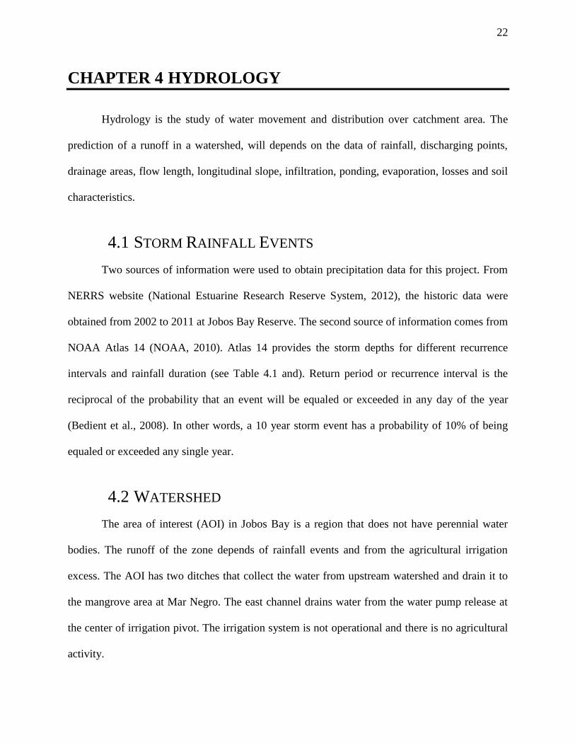
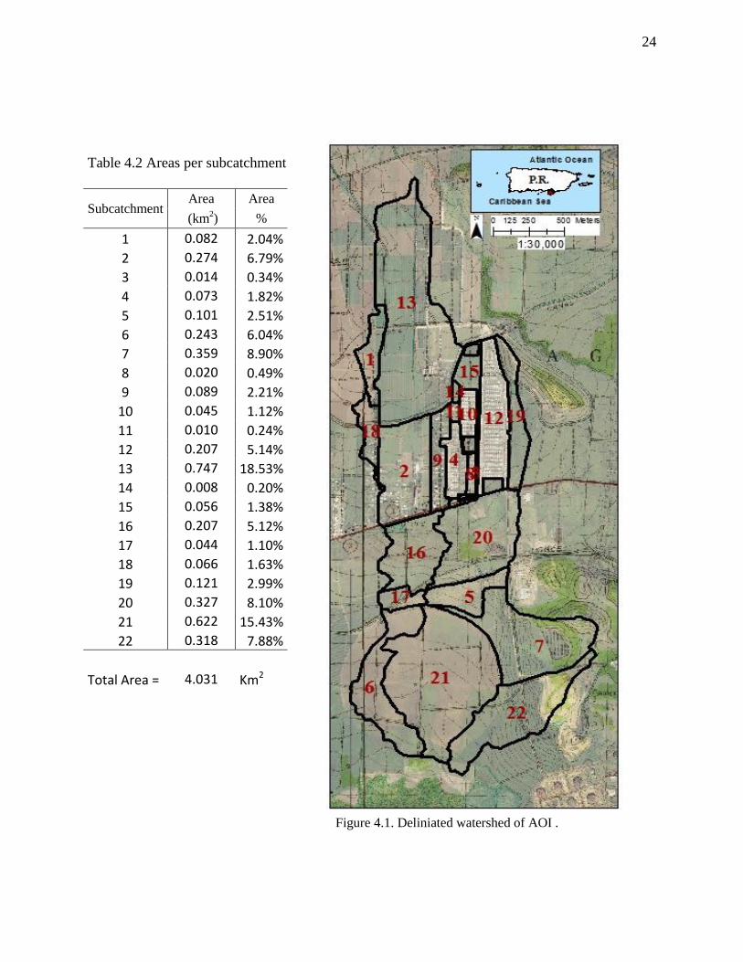
The west channel collects water from other places due to topographic features. Both
channels collect excess water from irrigation during agricultural activities and also drain waters
from nearby places. These two channels serve as starting point of watershed delineation (see
Figure 4.1). The watershed contributing to these channels starts in the AOI and extends 4.6 km to
the north along the valley with an area of about 4.0 km2.
The watershed delineation was prepared using ArcGIS 10 with a 1962 USGS digital
topographic map (Central Aguirre Quadrangle). The subwatersheds (see Figure 4.1) details were
obtained using overlapping of aerial photos4 from 2007 with a digital USGS topographic maps
and fieldwork. A total of 22 subcatchments were delineated according to the existing land use
and land cover of the area. Table 4.2 shows the area of each subcatchment.
4 Aerial photos from Central Aguirre and Salinas; United State Corps of Engineers, Spatial Resolution of 30 m.
Average recurrence interval (years)
Duration 1 2 5 10 25 50 100
5-mi 9 12 15 17 19 21 23 10-min 12 17 20 23 26 29 32 15-mi 16 21 26 29 34 37 41 30 - min 25 34 41 47 54 59 65 60 min 38 51 61 69 80 88 97 2-hr 46 65 82 95 113 127 141 3-hr 55 71 92 108 131 148 167 6-hr 67 88 118 143 177 205 234 12-hr 79 105 146 180 229 271 314 24-hr 93 123 176 221 287 343 403
Table 4.1 Precipitation partial duration series–based precipitation frecuency estimates (in
millimeters) at Salinas, P.R. Lat. 17.9702; Long.-66.2061– Guayama-Salinas, P.R
24
Table 4.2 Areas per subcatchment
Subcatchment Area Area
(km2) %
1 0.082 2.04%
2 0.274 6.79%
3 0.014 0.34%
4 0.073 1.82%
5 0.101 2.51%
6 0.243 6.04%
7 0.359 8.90%
8 0.020 0.49%
9 0.089 2.21%
10 0.045 1.12%
11 0.010 0.24%
12 0.207 5.14%
13 0.747 18.53%
14 0.008 0.20%
15 0.056 1.38%
16 0.207 5.12%
17 0.044 1.10%
18 0.066 1.63%
19 0.121 2.99%
20 0.327 8.10%
21 0.622 15.43%
22 0.318 7.88%
Total Area = 4.031 Km2
Figure 4.1. Deliniated watershed of AOI .
25
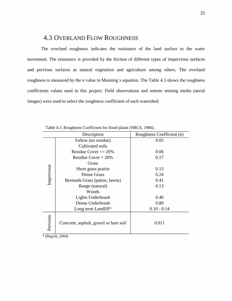
The overland roughness indicates the resistance of the land surface to the water
movement. The resistance is provided by the friction of different types of impervious surfaces
and pervious surfaces as natural vegetation and agriculture among others. The overland
roughness is measured by the n value in Manning`s equation. The Table 4.3 shows the roughness
coefficients values used in this project. Field observations and remote sensing media (aerial
images) were used to select the roughness coefficient of each watershed.
Description Roughness Coefficient (n)
Imper
vio
us
Fallow (no residue) 0.05
Cultivated soils
Residue Cover <= 20% 0.06
Residue Cover > 20% 0.17
Grass
Short grass prairie 0.15
Dense Grass 0.24
Bermuda Grass (patios, lawns) 0.41
Range (natural) 0.13
Woods
Lights Underbrush 0.40
Dense Underbrush 0.80
Long term Landfill* 0.10 - 0.14
Per
vio
us
Concrete, asphalt, gravel or bare soil 0.011
* (Bagchi, 2004)
4.3 OVERLAND FLOW ROUGHNESS
Table 4.3. Roughness Coefficient for flood plains (NRCS, 1986).

26
The hydrologic abstractions consist of the withdrawal of water from the hydrologic cycle
by evapotranspiration, ponding and infiltration. Evapotranspiration data was ignored for this
project due of the lack of information during analyzed periods. Evaporation data was not
available for this project. The watershed does not have natural ponding areas. There are three
small manmade retention ponds that have no effects on routing.
The infiltration is the capacity of the soil to let the water enter into it. Infiltration depends
on the soil properties determined mainly by the grain size distribution. Small grains size
corresponds to less infiltration. Infiltration can be also affected by a change in the bulk density,
and organic matter. If the bulk density increases, the amount of water retention decreases (Rawis,
et al. 1992). Infiltration is the major component of hydrologic abstractions.
The Curve Number (CN) method is used to estimate the runoff obtained from rainfall after
subtracting the hydrologic abstraction. The CNs were calculated by using the NRCS Web Soil
Survey (WSS, N.R.C.S., 2013) to obtain the hydrologic soil group and detailed land uses. The
hydrologic soil group was obtained through the input of the AOI delineated watershed to the WSS
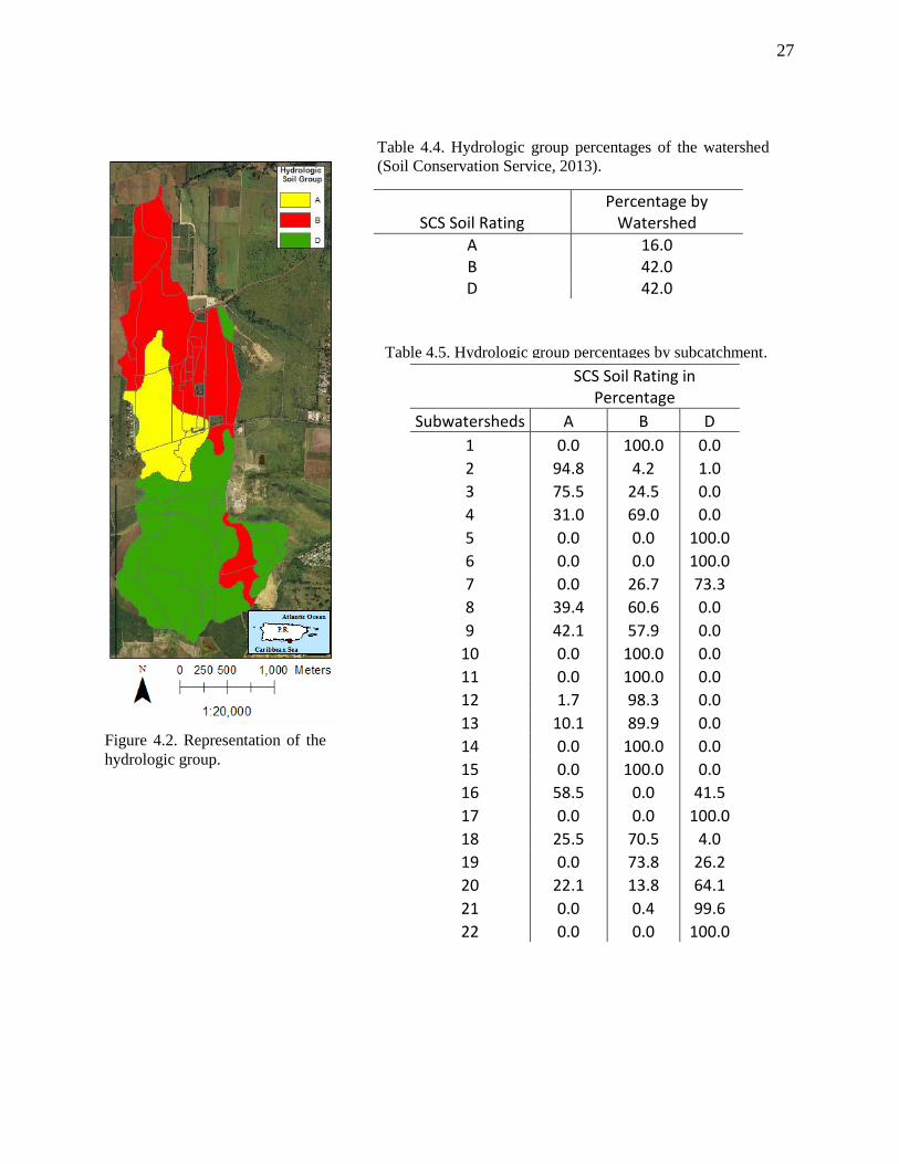
webpage, using a watershed shapefile created in ArcGIS (see Figure 4.1). The subcatchment (see
Figure 4.2) has three hydrologic groups which are: sandy loam - group A with a 16% of the
watershed, silty clay loam – group B with a 42% and clay soil – group D with the 42% of the
watershed. According to NRCS the predominant type of soil in the delineated watershed are clay
soils but each subcatchment can contain their own subdivision of hydrologic soils rating as shown in
Table 4.4. Details of the distribution of the hydrologic groups by subwatersheds in percentage are
shown in the Table 4.5.
4.4 HYDROLOGIC ABSTRACTION
27
SCS Soil Rating Percentage by
Watershed
A 16.0 B 42.0 D 42.0
SCS Soil Rating in Percentage
Subwatersheds A B D
1 0.0 100.0 0.0
2 94.8 4.2 1.0
3 75.5 24.5 0.0
4 31.0 69.0 0.0
5 0.0 0.0 100.0
6 0.0 0.0 100.0
7 0.0 26.7 73.3
8 39.4 60.6 0.0
9 42.1 57.9 0.0
10 0.0 100.0 0.0
11 0.0 100.0 0.0
12 1.7 98.3 0.0
13 10.1 89.9 0.0
14 0.0 100.0 0.0
15 0.0 100.0 0.0
16 58.5 0.0 41.5
17 0.0 0.0 100.0
18 25.5 70.5 4.0
19 0.0 73.8 26.2
20 22.1 13.8 64.1
21 0.0 0.4 99.6
22 0.0 0.0 100.0
Table 4.4. Hydrologic group percentages of the watershed
(Soil Conservation Service, 2013).
Figure 4.2. Representation of the
hydrologic group.
Table 4.5. Hydrologic group percentages by subcatchment.

28
The land uses were obtained from the WSS webpage, satellite imagery and field work
inspections. This field inspection involved recognition of the land use in the area, especially those
communities located at the north of the AOI watershed. Also, the field work helped to recognize the
communities’ water drain direction, water drainage outfalls, and which communities collect the water
in retention ponds.
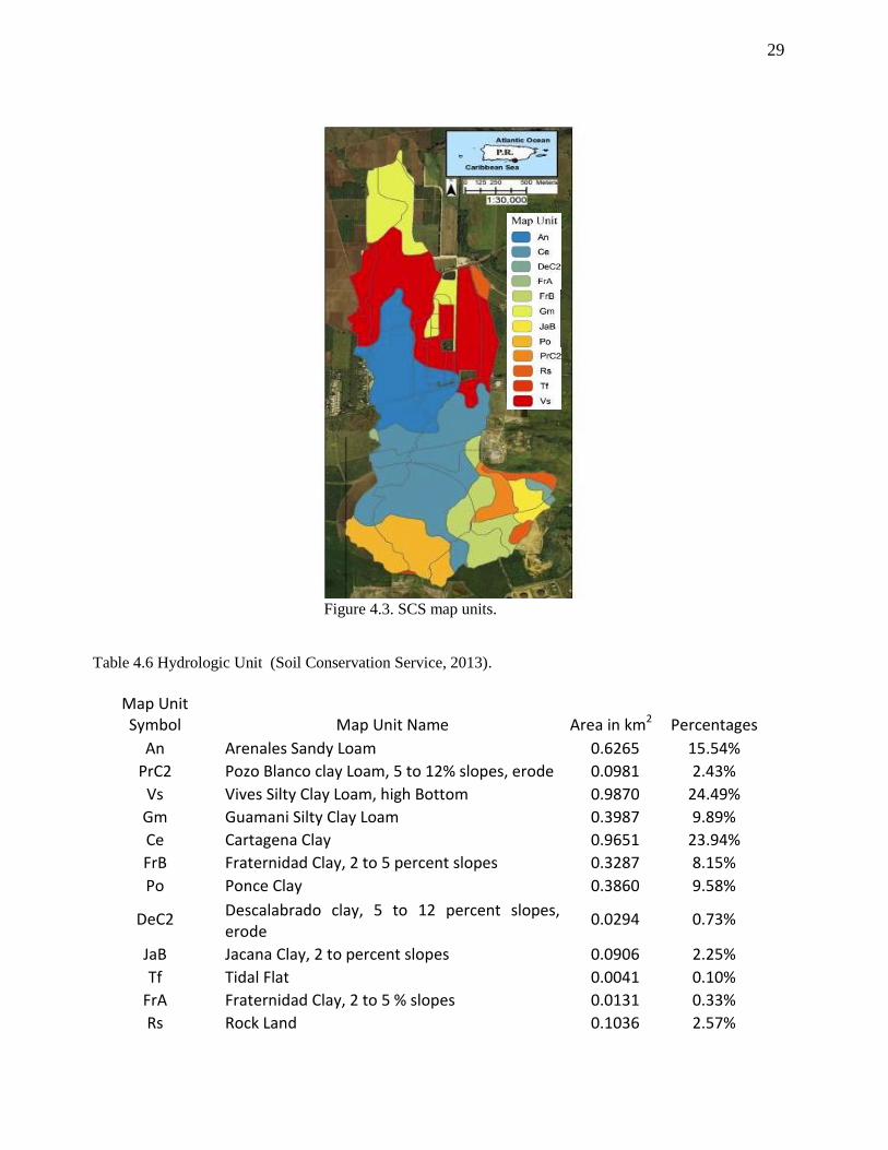
The unit soil groups were obtained from the WSS which are described in Table 4.6 and
Figure 4.3. The SCS National Engineering Handbook (Mockus, 2004) was used for identification
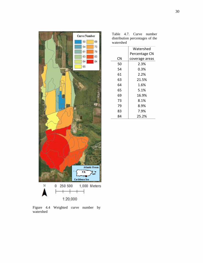
of the CN value by subcatchments. After obtained all the values of CN of each subcatchment, the
weighted CN method was used to compute the CN values using a composite weighted CN as
shown in Equation 4.1. The distribution of CN values in the watershed is shown in Figure 4.4. In
general the watershed has a minimum CN value of 50 a maximum of 84 which represent the
25% of the area (see Table 4.7).
where Ai is the area of each hydrologic unit inside one subcatchment and AT is the entire area of
that catchment.
∑
4.1
29
Table 4.6 Hydrologic Unit (Soil Conservation Service, 2013).
Map Unit Symbol Map Unit Name Area in km2 Percentages
An Arenales Sandy Loam 0.6265 15.54%
PrC2 Pozo Blanco clay Loam, 5 to 12% slopes, erode 0.0981 2.43%
Vs Vives Silty Clay Loam, high Bottom 0.9870 24.49%
Gm Guamani Silty Clay Loam 0.3987 9.89%
Ce Cartagena Clay 0.9651 23.94%
FrB Fraternidad Clay, 2 to 5 percent slopes 0.3287 8.15%
Po Ponce Clay 0.3860 9.58%
DeC2 Descalabrado clay, 5 to 12 percent slopes, erode
0.0294 0.73%
JaB Jacana Clay, 2 to percent slopes 0.0906 2.25%
Tf Tidal Flat 0.0041 0.10%
FrA Fraternidad Clay, 2 to 5 % slopes 0.0131 0.33%
Rs Rock Land 0.1036 2.57%
Figure 4.3. SCS map units.
30
Table 4.7. Curve number
distribution percentages of the
watershed
CN
Watershed Percentage CN coverage areas
50 2.3%
54 0.3%
61 2.2%
63 21.5%
64 1.6%
65 5.1%
69 16.9%
73 8.1%
79 8.9%
83 7.9%
84 25.2%
Figure 4.4 Weighted curve number by
watershed
31
Historical rainfall data was obtained from NOAA National Estuarine Research Reserve
website for the meteorological Station Jobos Bay weather (SJB) located in latitude
17°57'23.25"N and longitude 66°13'22.69"W (National Estuarine Research Reserve System,
2012). The SJB is situated approximately 2.5 kilometers to the east of the study area. This station
provides information from 2002 to present in periods of 15 minutes. Only the data from 2002 to
2011 was analyzed. These data was processed to obtain the maximum accumulation of rain in a
period of 24 hours every year.
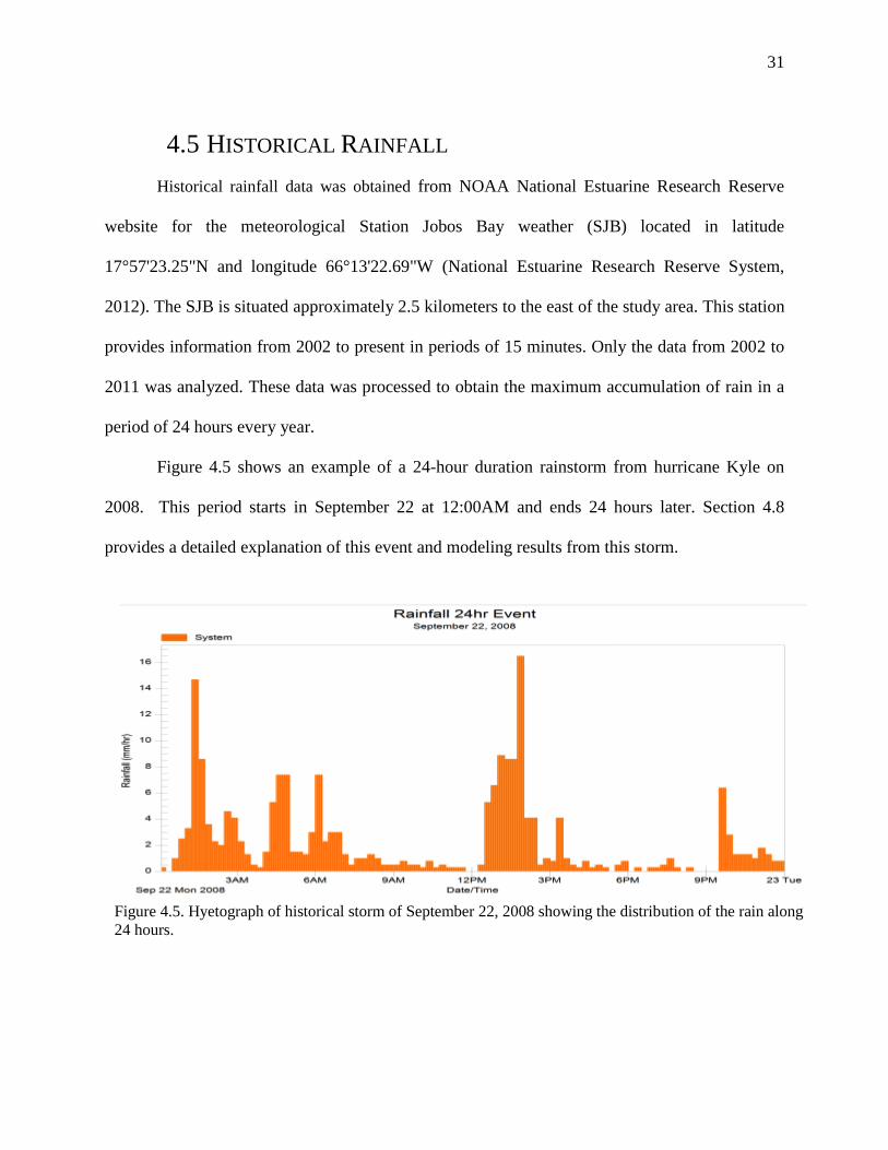
Figure 4.5 shows an example of a 24-hour duration rainstorm from hurricane Kyle on
2008. This period starts in September 22 at 12:00AM and ends 24 hours later. Section 4.8
provides a detailed explanation of this event and modeling results from this storm.
4.5 HISTORICAL RAINFALL
Figure 4.5. Hyetograph of historical storm of September 22, 2008 showing the distribution of the rain along
24 hours.
32
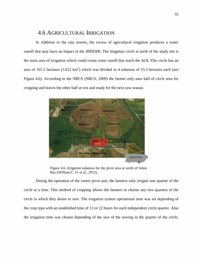
In Addition to the rain storms, the excess of agricultural irrigation produces a water
runoff that may have an impact in the JBNERR. The irrigation circle at north of the study site is
the main area of irrigation which could create some runoff that reach the AOI. This circle has an
area of 101.2 hectares (1.012 km2) which was divided in 4 subareas of 25.3 hectares each (see
Figure 4.6). According to the NRCS (NRCS, 2009) the farmer only uses half of circle area for
cropping and leaves the other half at rest and ready for the next sow season.
During the operation of the center pivot unit, the farmers only irrigate one quarter of the
circle at a time. This method of cropping allows the farmers to choose any two quarters of the
circle in which they desire to sow. The irrigation system operational time was set depending of
the crop type with an established time of 13 or 22 hours for each independent circle quarter. Also
the irrigation time was chosen depending of the size of the sowing in the quarter of the circle.
4.6 AGRICULTURAL IRRIGATION
Figure 4.6. Irrigation subareas for the pivot area at north of Jobos
Bay (William C. O. et al., 2012).
AOI
33
The corn crops were the only sow, which requires an irrigation of 22 hours twice a week (NRCS,
2009).
During the years of 2008 and 2009 crops of corn, cowpea and sorghum were sowed and
irrigated using the pivot unit system (Williams et al., 2012). The sorghum crops require an
irrigation of 9.14 millimeters per day, while the corn crops needs 9.89 millimeters per day
(NRCS, 2009). The irrigation data correspond to the peak season during the months of July and
August. The annual irrigation amount for 2008 and 2009 were 553 millimeters and 1270
millimeters, respectively (William C. O. et al., 2012). Also the amounts of rain for the same
years were 1059 mm and 670 mm, respectively. Irrigation flows were considered as inflow in the
design as explained in Section 4.8.
The Storm Water Management Model (SWMM) developed by U.S. Environmental
Protection Agency (EPA) was selected as design tool for this project. SWMM allows full
integration of hydrology and hydraulic design on detailed scale and complex spatially, and
temporal varied flow conditions (Environmental Protection Agency, 2013). SWMM is an
enhanced version of US EPA storm water management model (CHI, 2011) that includes a self-
contained GIS interphase for spatial analysis.
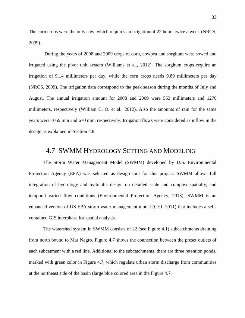
The watershed system in SWMM consists of 22 (see Figure 4.1) subcatchments draining
from north bound to Mar Negro. Figure 4.7 shows the connection between the preset outlets of
each subcatment with a red line. Additional to the subcatchments, there are three retention ponds,
marked with green color in Figure 4.7, which regulate urban storm discharge from communities
at the northeast side of the basin (large blue colored area in the Figure 4.7.
4.7 SWMM HYDROLOGY SETTING AND MODELING
34
The basin has two principal subcatchments, one at the east side which includes the
communities and the west side which has low density communities and more agricultural areas.
Both watersheds drain toward the south discharging into the two earth channels named West
Channel and East Channel (see Figure 1.2).
Historic rainfall data gives an idea of the amount of precipitation occurring in the area.
The last ten years rainfall data was chosen for this analysis, (2002 -2011); The first step was to
find the highest cumulative precipitation in 24hrs by year, starting at 12:00 AM (see hyetographs
in Appendix B). With the sorted data, identify if the storm date was related to a meteorological
system was performed (as a tropical storm, hurricane, etc.). If the storm has relation with a
4.8 HYDROLOGIC ANALYSIS
Figure 4.7. PCSWMM maximum surface
runoff by subcatchment.
Legend
Link
Retention
Pond
Joint
Urban
area
Watershed
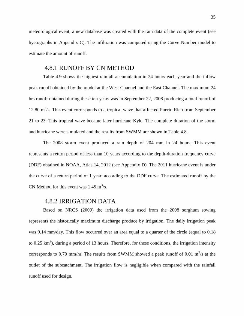
35
meteorological event, a new database was created with the rain data of the complete event (see
hyetographs in Appendix C). The infiltration was computed using the Curve Number model to
estimate the amount of runoff.
Table 4.9 shows the highest rainfall accumulation in 24 hours each year and the inflow
peak runoff obtained by the model at the West Channel and the East Channel. The maximum 24
hrs runoff obtained during these ten years was in September 22, 2008 producing a total runoff of
12.80 m3/s. This event corresponds to a tropical wave that affected Puerto Rico from September
21 to 23. This tropical wave became later hurricane Kyle. The complete duration of the storm
and hurricane were simulated and the results from SWMM are shown in Table 4.8.
The 2008 storm event produced a rain depth of 204 mm in 24 hours. This event
represents a return period of less than 10 years according to the depth-duration frequency curve
(DDF) obtained in NOAA, Atlas 14, 2012 (see Appendix D). The 2011 hurricane event is under
the curve of a return period of 1 year, according to the DDF curve. The estimated runoff by the
CN Method for this event was 1.45 m3/s.
Based on NRCS (2009) the irrigation data used from the 2008 sorghum sowing
represents the historically maximum discharge produce by irrigation. The daily irrigation peak
was 9.14 mm/day. This flow occurred over an area equal to a quarter of the circle (equal to 0.18
to 0.25 km2), during a period of 13 hours. Therefore, for these conditions, the irrigation intensity
corresponds to 0.70 mm/hr. The results from SWMM showed a peak runoff of 0.01 m3/s at the
outlet of the subcatchment. The irrigation flow is negligible when compared with the rainfall
runoff used for design.
4.8.1 RUNOFF BY CN METHOD
4.8.2 IRRIGATION DATA
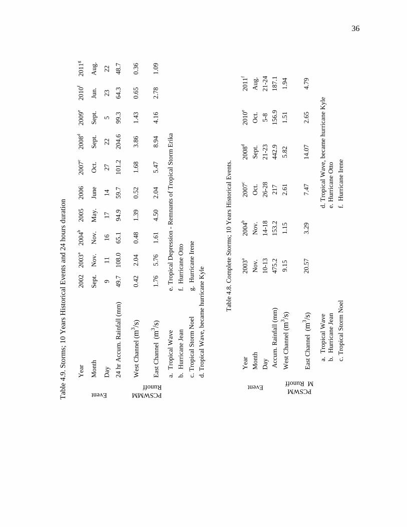
36
Tab
le 4
.9. S
torm
s; 1
0 Y
ears
His
tori
cal
Even
ts a
nd 2
4 h
ours
dura
tion
Event
Yea
r 2
00
2
20
03
a 2
00
4b
20
05
20
06
20
07
c 2
00
8d
20
09
e 2
01
0f
20
11
g
Mo
nth
S
ept.
N
ov.
No
v.
May.
June
Oct
. S
ept.
S
ept.
Ju
n.
Au
g.
Day
9
11
16
17
14
27
22
5
23
22
2
4 h
r A
ccu
m.
Rai
nfa
ll (
mm
) 4
9.7
1
08
.0
65
.1
94
.9
59
.7
10
1.2
2
04
.6
99
.3
64
.3
48
.7
PCSWMM
Runoff W
est
Chan
nel
(m
3/s
) 0
.42
2.0
4
0.4
8
1.3
9
0.5
2
1.6
8
3.8
6
1.4
3
0.6
5
0.3
6
Eas
t C
han
nel
(m
3/s
) 1
.76
5.7
6
1.6
1
4.5
0
2.0
4
5.4
7
8.9
4
4.1
6
2.7
8
1.0
9
a.
T
rop
ical
Wav
e e.
Tro
pic
al D
epre
ssio
n -
Rem
nan
ts o
f T
rop
ical
Sto
rm E
rika
b
. H
urr
ican
e Je
an
f.
Hurr
ican
e O
tto
c.
Tro
pic
al S
torm
No
el
g.
Hurr
ican
e Ir
ene
d
. T
rop
ical
Wav
e, b
ecam
e h
urr
ican
e K
yle
Tab
le 4
.8. C
om
ple
te S
torm
s; 1
0 Y
ears
His
tori
cal
Even
ts.
Event
Yea
r 2
00
3a
20
04
b
20
07
c 2
00
8d
20
10
e 2
01
1f
Mo
nth
N
ov.
No
v.
Oct
. S
ept.
O
ct.
Au
g.
Day
10
-13
14
-18
26
-28
21
-23
5-8
2
1-2
4
A
ccu
m.
Rai
nfa
ll (
mm
) 4
75
.2
15
3.2
2
17
44
2.9
1
56
.9
18
7.1
PCSWM
M Runoff
Wes
t C
han
nel
(m
3/s
) 9
.15
1.1
5
2.6
1
5.8
2
1.5
1
1.9
4
Eas
t C
han
nel
(m
3/s
) 2
0.5
7
3.2
9
7.4
7
14
.07
2
.65
4.7
9
a.
Tro
pic
al W
ave
d. T
rop
ical
Wav
e, b
ecam
e h
urr
ican
e K
yle
b.
Hurr
ican
e Je
an
e.
Hurr
ican
e O
tto
c.
Tro
pic
al S
torm
No
el
f.
Hurr
ican
e Ir
ene
37
CHAPTER 5 HYDRAULICS
The rainfall chosen for hydraulic design was the 2011 maximum 24 hr duration storm
event with an accumulative rainfall of 48.7 mm. This rainfall event produced a peak runoff of
0.36 m3/s for the West Channel and 1.09 m
3/s for the East Channel (see last column of Table
4.9). This event produced the minimum flow among the 10 rainfall events analyzed in SWMM.
Larger events flooded the area completely making unnecessary a design for peak flows
exceeding one-year frequency.
The Jobos watershed has multiple irrigation channels which drains the excess water from
the crops areas to Jobos Bay (see Figure 2.1.B). They were excavated by the P.R. Land Authority
to control the excess of water from furrow irrigation systems during the sugar cane production
times (Gregory L. Morris & Associates, 2000). Two of these channels (see Figure 1.2) drain
water from a pivot irrigation system to Mar Negro.
These channels were named East Channel and West Channel, due to their location, from
the center of the area of interest. The West Channel collects water which drains from the west
side of the pivot. The length of this channel is 220 m until it reaches the area of interest (AOI).
This channel has a trapezoidal geometry with a variable depth which increases aproximately 1.5
m in the transition zone between the JBNERR region and PRLA lands. In the JBNERR area, the
channel depth is 0.4 meter depth before it discharges into the Mar Negro. The top width of the
channels varies from 5.5 m in the deepest areas to 3 m in the outlet to Mar Negro. The bottom of
the existing channels is composed of silt and clay, organic material and some areas are covered
with vegetation. Most of this vegetation can be found in the transition zone upstream of the study
area.
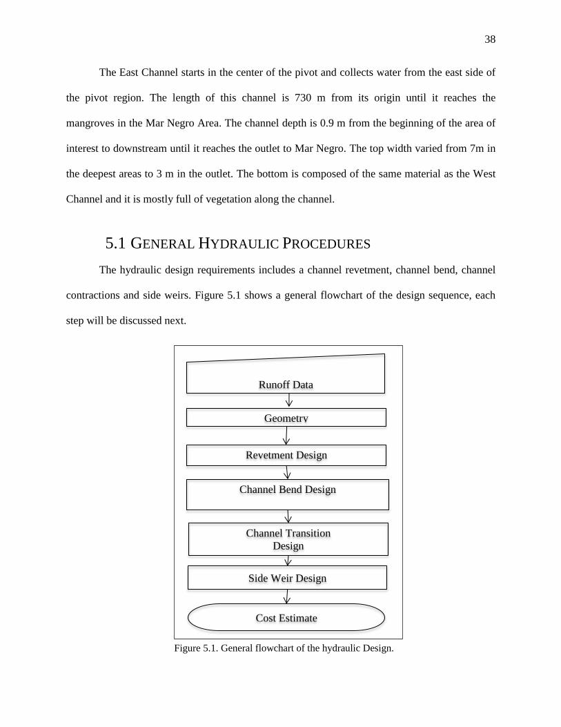
38
The East Channel starts in the center of the pivot and collects water from the east side of
the pivot region. The length of this channel is 730 m from its origin until it reaches the
mangroves in the Mar Negro Area. The channel depth is 0.9 m from the beginning of the area of
interest to downstream until it reaches the outlet to Mar Negro. The top width varied from 7m in
the deepest areas to 3 m in the outlet. The bottom is composed of the same material as the West
Channel and it is mostly full of vegetation along the channel.
The hydraulic design requirements includes a channel revetment, channel bend, channel
contractions and side weirs. Figure 5.1 shows a general flowchart of the design sequence, each
step will be discussed next.
5.1 GENERAL HYDRAULIC PROCEDURES
Geometry
Runoff Data
Revetment Design
Channel Bend Design
Channel Transition
Design
Side Weir Design
Cost Estimate
Figure 5.1. General flowchart of the hydraulic Design.

39
The project watershed does not have any perennial water stream network. The only drainage
system that has the watershed is a series of channels that were built to discharge the excess of
agricultural irrigation.
Water from the East and West Channel will be collected in two independents new channels.
Each new channel will redirect the water parallel to the bay coastline and spread it as overland
flow by using a set of lateral weirs. Channel dimensions were adjusted such that an almost equal
amount of water can be spreaded along the channel. The system will distribute runoff and
irrigation water over the AOI, promoting vegetation, filtrating pesticides and fertilizers from
agricultural activities and reducing impact of chemicals reaching the mangrove area by spreading
the discharge from the farmlands.
The new design consist of a variable geometry channel, reducing channel bottom width from
three meters to one half meter. All sections are trapezoidal with a side slope of 1:1.5 for stability
purposes. There is a transition between each section and three lateral weirs are designed at each
channel reach. Figure 5.2 and Table 5.1 presents the description of the general geometry along
both channels, East and West Channel.
The flow varies gradually along of the channel, due to the side weirs and transition sections
produce a water depth variation along the channel section. The computation of the water depth
starts at the last downstream side weir (see Figure 5.2), where a known depth is fixed at 0.37 m
for the West Channel and 0.62 m for East Channel, as a boundaries condition. These initial
depths were obtained by the computation of the normal depth in the upstream side of the weir.
Computation continues to the next upstream section.
5.2 CHANNELS CHARACTERISTICS AND SIDE WEIRS DESIGN
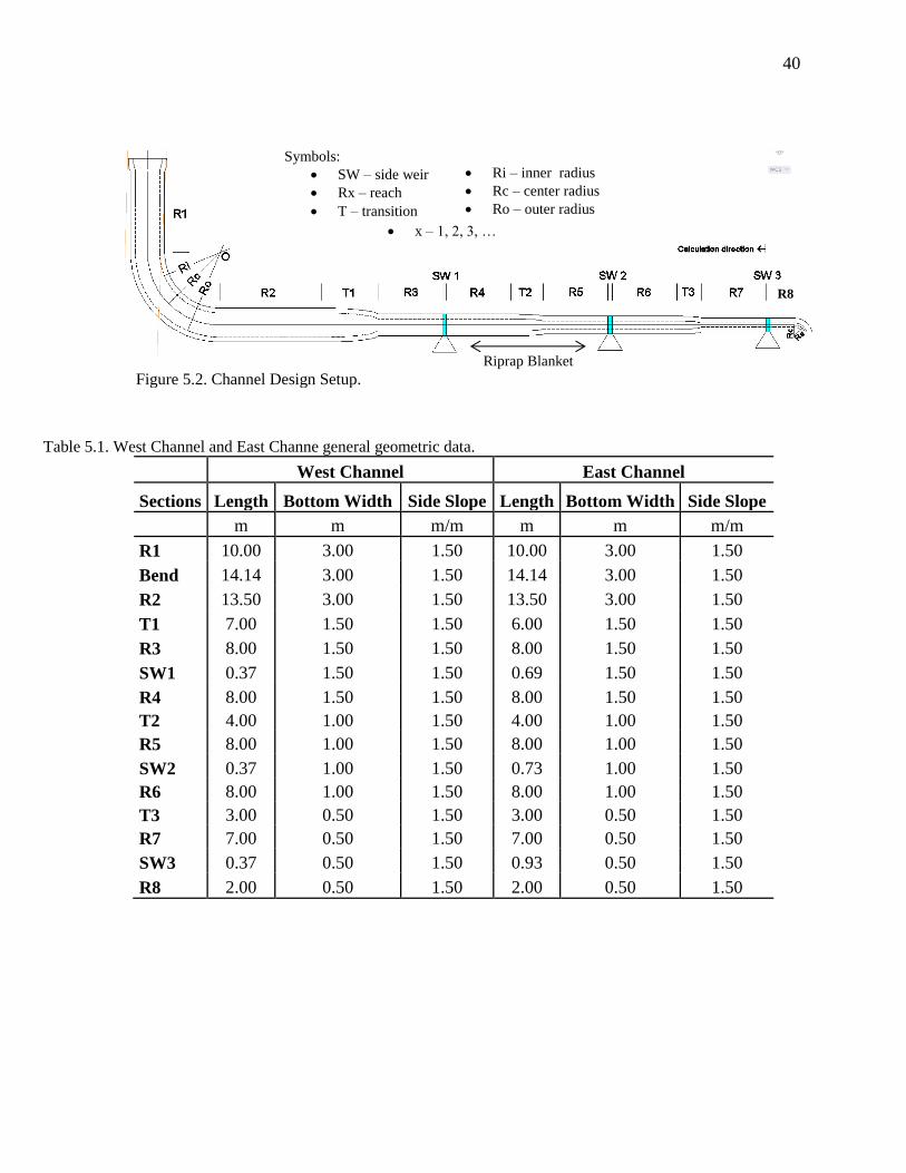
40
Table 5.1. West Channel and East Channe general geometric data.
West Channel East Channel
Sections Length Bottom Width Side Slope Length Bottom Width Side Slope
m m m/m m m m/m
R1 10.00 3.00 1.50 10.00 3.00 1.50
Bend 14.14 3.00 1.50 14.14 3.00 1.50
R2 13.50 3.00 1.50 13.50 3.00 1.50
T1 7.00 1.50 1.50 6.00 1.50 1.50
R3 8.00 1.50 1.50 8.00 1.50 1.50
SW1 0.37 1.50 1.50 0.69 1.50 1.50
R4 8.00 1.50 1.50 8.00 1.50 1.50
T2 4.00 1.00 1.50 4.00 1.00 1.50
R5 8.00 1.00 1.50 8.00 1.00 1.50
SW2 0.37 1.00 1.50 0.73 1.00 1.50
R6 8.00 1.00 1.50 8.00 1.00 1.50
T3 3.00 0.50 1.50 3.00 0.50 1.50
R7 7.00 0.50 1.50 7.00 0.50 1.50
SW3 0.37 0.50 1.50 0.93 0.50 1.50
R8 2.00 0.50 1.50 2.00 0.50 1.50
Figure 5.2. Channel Design Setup.
Symbols:
SW – side weir
Rx – reach
T – transition
Ri – inner radius
Rc – center radius
Ro – outer radius
x – 1, 2, 3, …
Riprap Blanket
R8
41
During an open channel design it is important to consider the channel bed and banks
protection from erosion. The channel lining can provide the protection to walls and the channel
bed from erosion and decrease its maintenance cost. Unlined natural channels are generally
susceptible to erosion and development of vegetation inside the channel, increasing the
maintenance cost and deteriorating the operation of the channel. Other factor that needs to be
verified during the lining selection is the maximum velocity allowed by the type of lining. In
other words, the maximum water velocity allowed by the lining to prevent erosion (Chow, 1959)
or damage to the channel walls and bed. This section will introduce the types of linings that were
considered on this project.
Earth lining
This lining will depends to the soil type, flow velocity and requires continued
maintenance among other factors. Earth lining will be affected by erosion especially if the mean
velocity exceeds the 0.9 meter per second and the side slopes are less than 3H: 1V (City of EL
Paso, Engineering Department, 2008).
With this lining the East and West channels will experiment failures due to intermittent
drying and watering conditions. This type of channel requires constant maintenance which
increases the operational cost. Also, spill flow during some events will erode the channels walls
and alter the geometry of the side wall.
Concrete lining
The concrete lining channels may be constructed of reinforced concrete and is generally
used in rectangular channels or in trapezoidal channels. The use of steel to reinforce the structure
represents a cost increase in materials and construction of the system. This type of lining is
5.3 CHANNEL LINING
42
generally designed for supercritical flow conditions or velocities greater than 1.5 meter per
second. Side wall angles could be steeper than 2:1 (City of EL Paso, Engineering Department,
2008). This lining was not chosen for this project because this type of lining represents a high
construction cost. The channel will need to be reinforced completely specially in the areas of the
side weirs and at the transition. Velocity in this project are low, therefore, concrete lined is not
justified.
Riprap Lining
The riprap is used as erosion control lining for natural channels. The surface of this lining
is composed of rocks which increase channel roughness depending of rock size. This increase in
roughness allows the channel to handle more pronounced longitudinal gradients (Federal
Highway Administration, 1988). During a lack of maintenance, the riprap is susceptible to
growth of vegetation which represents an increase in flow resistance and decreases the channel
capacity. The maximum allowed side slope is 3H: 1V. The riprap lining is one option for this
project but, the channel will be exposed to vegetation growth. As previously mentioned the
vegetation can offer a resistance to the water and affect the operation of the weirs channel and
the rest of the channel.
Grouted riprap lining
This type of lining provides a rigid surface because the riprap is grouted. The benefit to
have a grouted material is that the lining can use a smaller size of riprap. Also the maintenance
of the channel is less than other linings. Since the walls and the channel bed are grouted an
impermeable layer is created which do not allow the groundwater pressure being released
between the rocks (WEF and ASCE, 1992). This lining prevents channel erosion and the grouted
produces an impermeable layer which protects the channel bed and sidewall from vegetation
43
growth. This option of lining has the best characteristics for the design purposes of this project
and was selected.
Riprap is a lining formed by large angular rocks which provide soil protection from
erosion and decreases the runoff velocities. The lining design calculations are based on a
trapezoidal shape channel covered of cement mortar. The cement mortar layer increases the shear
stress resistance, provides stability, and prevents vegetation growth inside of the channel. This is
called grouted riprap lining, which is recommended for this project. This type of lining provides
stability to the walls and bottom of the channel and reduce maintenance cost. Also, the use of a
concrete mortar to stick the rocks to the channel surface allows to use a smaller riprap size.
There are several methods for riprap design. This project used the method proposed by
the National Cooperative Highway Research Program (NCHRP) Report 108, 1970 (Anderson et
al., 1970 and Sturm, 2011). This method describes step by step the design of riprap lining to
prevent erosion of highway drainage channels. This method involves channel geometry,
longitudinal slope, roughness coefficient, the mean riprap size, shear stress exerted on the
channel bed and the sidewalls, and the design discharge.
The riprap design criteria are that the maximum shear stress (MSS) exerted by the water
on the channel walls ( and bed , does not exceed the critical shear stress (CSS) at both
places. Figure 5.3 shows a flowchart with the procedure to select a riprap size. Each step of the
flow chart will be discussed in detail in this section.
5.4 RIPRAP – LINING CHANNEL DESIGN PROCEDURES
5.4.1 RIPRAP DESIGN CRITERIA
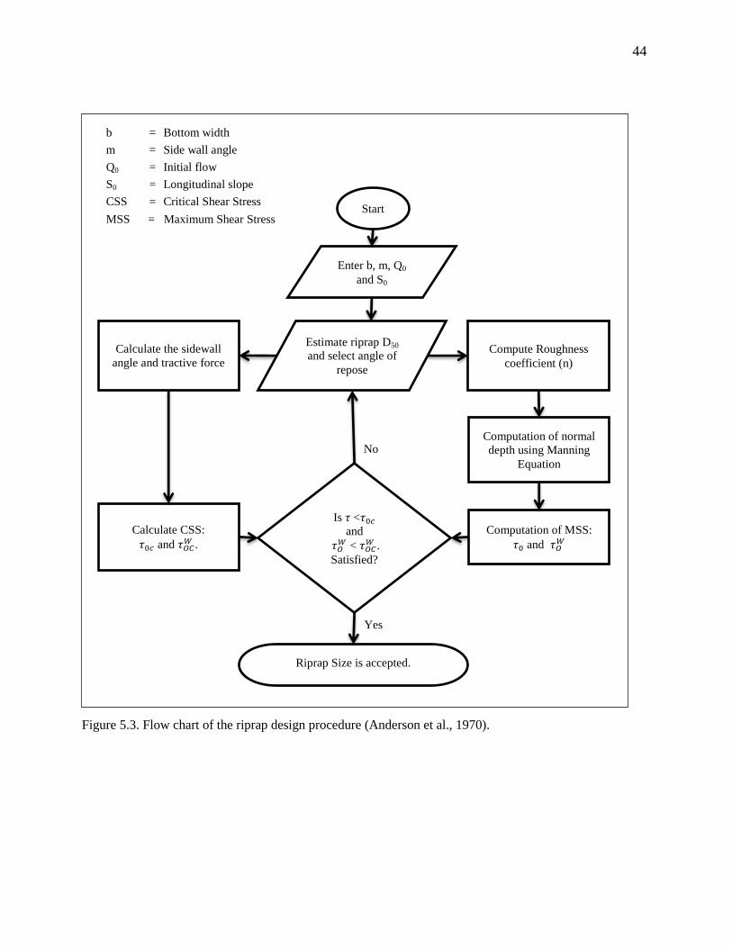
44
No
Yes
Start
Enter b, m, Q0
and S0
Is 𝜏 <𝜏 𝑐
and
𝜏𝑂𝑊 < 𝜏𝑂𝐶
𝑊 .
Satisfied?
Compute Roughness
coefficient (n)
Estimate riprap D50
and select angle of
repose
Calculate CSS:
𝜏 𝑐 and 𝜏𝑂𝐶𝑊 .
Calculate the sidewall
angle and tractive force
Computation of normal
depth using Manning
Equation
Computation of MSS:
𝜏 and 𝜏𝑂𝑊
Riprap Size is accepted.
Figure 5.3. Flow chart of the riprap design procedure (Anderson et al., 1970).
b = Bottom width
m = Side wall angle
Q0 = Initial flow
S0 = Longitudinal slope
CSS = Critical Shear Stress
MSS = Maximum Shear Stress
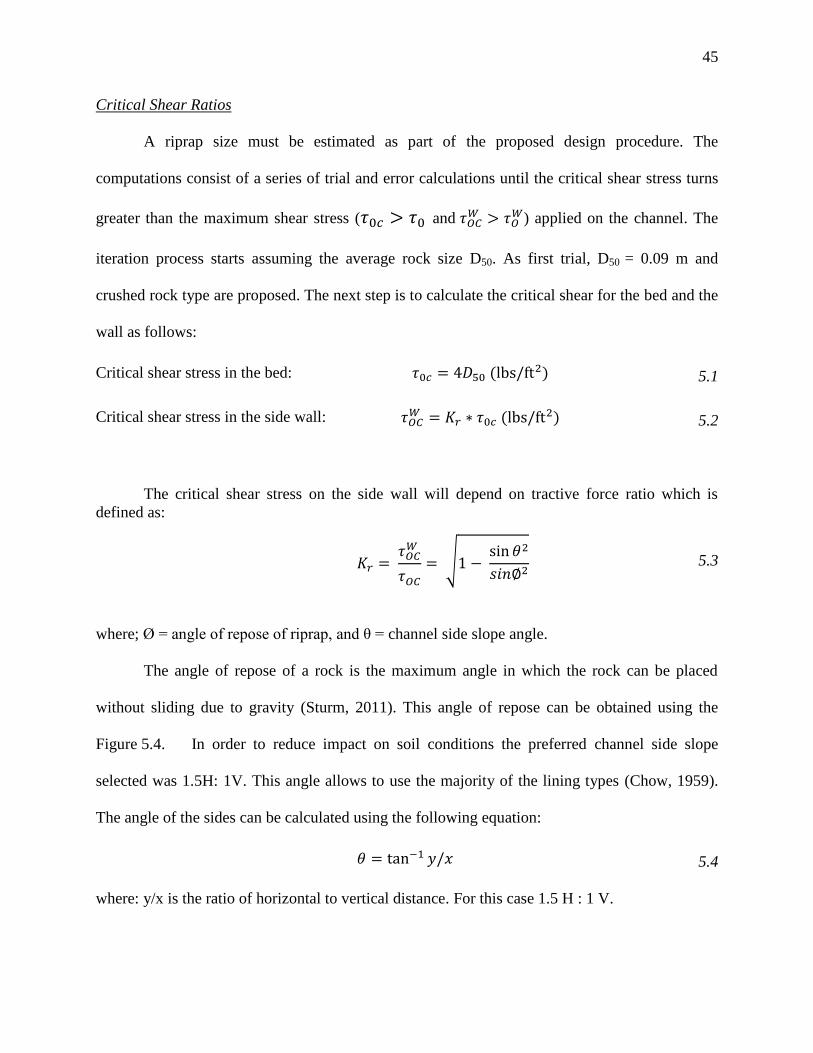
45
Critical Shear Ratios
A riprap size must be estimated as part of the proposed design procedure. The
computations consist of a series of trial and error calculations until the critical shear stress turns
greater than the maximum shear stress ( and
) applied on the channel. The
iteration process starts assuming the average rock size D50. As first trial, D50 = 0.09 m and
crushed rock type are proposed. The next step is to calculate the critical shear for the bed and the
wall as follows:
Critical shear stress in the bed: 5.1
Critical shear stress in the side wall:
5.2
The critical shear stress on the side wall will depend on tractive force ratio which is
defined as:
where; Ø = angle of repose of riprap, and θ = channel side slope angle.
The angle of repose of a rock is the maximum angle in which the rock can be placed
without sliding due to gravity (Sturm, 2011). This angle of repose can be obtained using the
Figure 5.4. In order to reduce impact on soil conditions the preferred channel side slope
selected was 1.5H: 1V. This angle allows to use the majority of the lining types (Chow, 1959).
The angle of the sides can be calculated using the following equation:
5.4
where: y/x is the ratio of horizontal to vertical distance. For this case 1.5 H : 1 V.
√
5.3
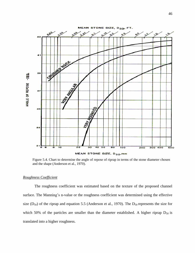
46
Roughness Coefficient
The roughness coefficient was estimated based on the texture of the proposed channel
surface. The Manning’s n-value or the roughness coefficient was determined using the effective
size (D50) of the riprap and equation 5.5 (Anderson et al., 1970). The D50 represents the size for
which 50% of the particles are smaller than the diameter established. A higher riprap D50 is
translated into a higher roughness.
Figure 5.4. Chart to determine the angle of repose of riprap in terms of the stone diameter chosen
and the shape (Anderson et al., 1970).
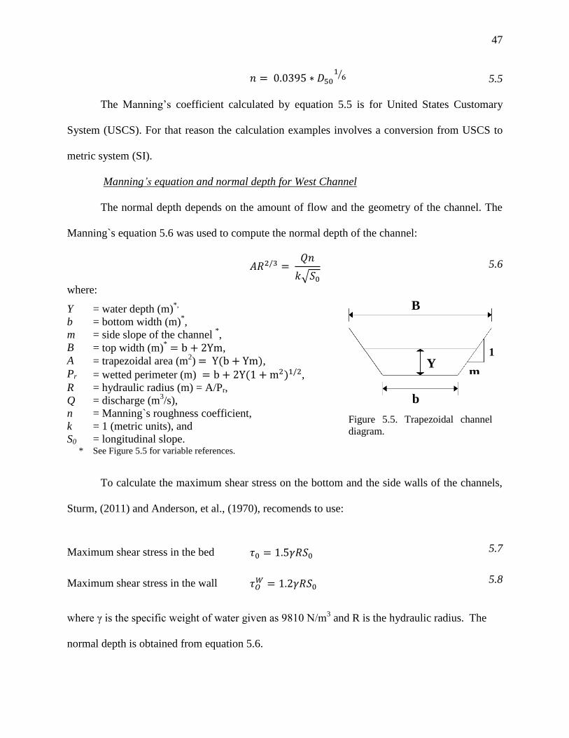
47
⁄ 5.5
The Manning’s coefficient calculated by equation 5.5 is for United States Customary
System (USCS). For that reason the calculation examples involves a conversion from USCS to
metric system (SI).
Manning’s equation and normal depth for West Channel
The normal depth depends on the amount of flow and the geometry of the channel. The
Manning`s equation 5.6 was used to compute the normal depth of the channel:
√
5.6
where:
To calculate the maximum shear stress on the bottom and the side walls of the channels,
Sturm, (2011) and Anderson, et al., (1970), recomends to use:
where γ is the specific weight of water given as 9810 N/m3 and R is the hydraulic radius. The
normal depth is obtained from equation 5.6.
Y
= water depth (m)*,
b
= bottom width (m)*,
m = side slope of the channel *,
B
= top width (m)* ,
A = trapezoidal area (m2) ,
Pr = wetted perimeter (m) ,
R = hydraulic radius (m) = A/Pr,
Q = discharge (m3/s),
n = Manning`s roughness coefficient,
k = 1 (metric units), and
S0 = longitudinal slope. * See Figure 5.5 for variable references.
Maximum shear stress in the bed 5.7
Maximum shear stress in the wall 5.8
Figure 5.5. Trapezoidal channel
diagram.
m
B
b
Y 1
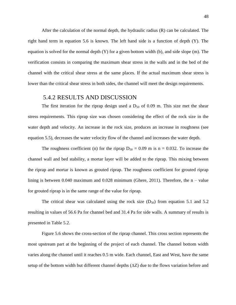
48
After the calculation of the normal depth, the hydraulic radius (R) can be calculated. The
right hand term in equation 5.6 is known. The left hand side is a function of depth (Y). The
equation is solved for the normal depth (Y) for a given bottom width (b), and side slope (m). The
verification consists in comparing the maximum shear stress in the walls and in the bed of the
channel with the critical shear stress at the same places. If the actual maximum shear stress is
lower than the critical shear stress in both sides, the channel will meet the design requirements.
The first iteration for the riprap design used a D50 of 0.09 m. This size met the shear
stress requirements. This riprap size was chosen considering the effect of the rock size in the
water depth and velocity. An increase in the rock size, produces an increase in roughness (see
equation 5.5), decreases the water velocity flow of the channel and increases the water depth.
The roughness coefficient (n) for the riprap D50 = 0.09 m is n = 0.032. To increase the
channel wall and bed stability, a mortar layer will be added to the riprap. This mixing between
the riprap and mortar is known as grouted riprap. The roughness coefficient for grouted riprap
lining is between 0.040 maximum and 0.028 minimum (Ghere, 2011). Therefore, the n – value
for grouted riprap is in the same range of the value for riprap.
The critical shear was calculated using the rock size (D50) from equation 5.1 and 5.2
resulting in values of 56.6 Pa for channel bed and 31.4 Pa for side walls. A summary of results is
presented in Table 5.2.
Figure 5.6 shows the cross-section of the riprap channel. This cross section represents the
most upstream part at the beginning of the project of each channel. The channel bottom width
varies along the channel until it reaches 0.5 m wide. Each channel, East and West, have the same
setup of the bottom width but different channel depths (∆Z) due to the flows variation before and
5.4.2 RESULTS AND DISCUSSION
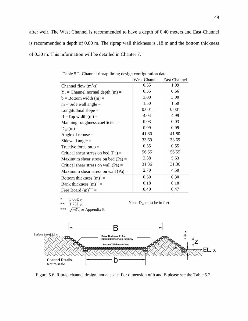
49
after weir. The West Channel is recommended to have a depth of 0.40 meters and East Channel
is recommended a depth of 0.80 m. The riprap wall thickness is .18 m and the bottom thickness
of 0.30 m. This information will be detailed in Chapter 7.
* 3.00D50.
** 1.75D50.
*** √ or Appendix E
West Channel East Channel
Channel flow (m3/s) 0.35 1.09
Yn = Channel normal depth (m) = 0.35 0.66
b = Bottom width (m) = 3.00 3.00
m = Side wall angle = 1.50 1.50
Longitudinal slope = 0.001 0.001
B =Top width (m) = 4.04 4.99
Manning roughness coefficient = 0.03 0.03
D50 (m) = 0.09 0.09
Angle of repose = 41.80 41.80
Sidewall angle = 33.69 33.69
Tractive force ratio = 0.55 0.55
Critical shear stress on bed (Pa) = 56.55 56.55
Maximum shear stress on bed (Pa) = 3.38 5.63
Critical shear stress on wall (Pa) = 31.36 31.36
Maximum shear stress on wall (Pa) = 2.70 4.50
Bottom thickness (m)* = 0.30 0.30
Bank thickness (m)**
= 0.18 0.18
Free Board (m)***
= 0.40 0.47
Table 5.2. Channel riprap lining design configuration data
Figure 5.6. Riprap channel design, not at scale. For dimension of b and B please see the Table 5.2
Channel Details
Not to scale
Bank Thickness 0.18 m
Riprap finished with concrete.
Bottom Thickness 0.30 m
0.1
50 m
Note: D50 must be in feet.
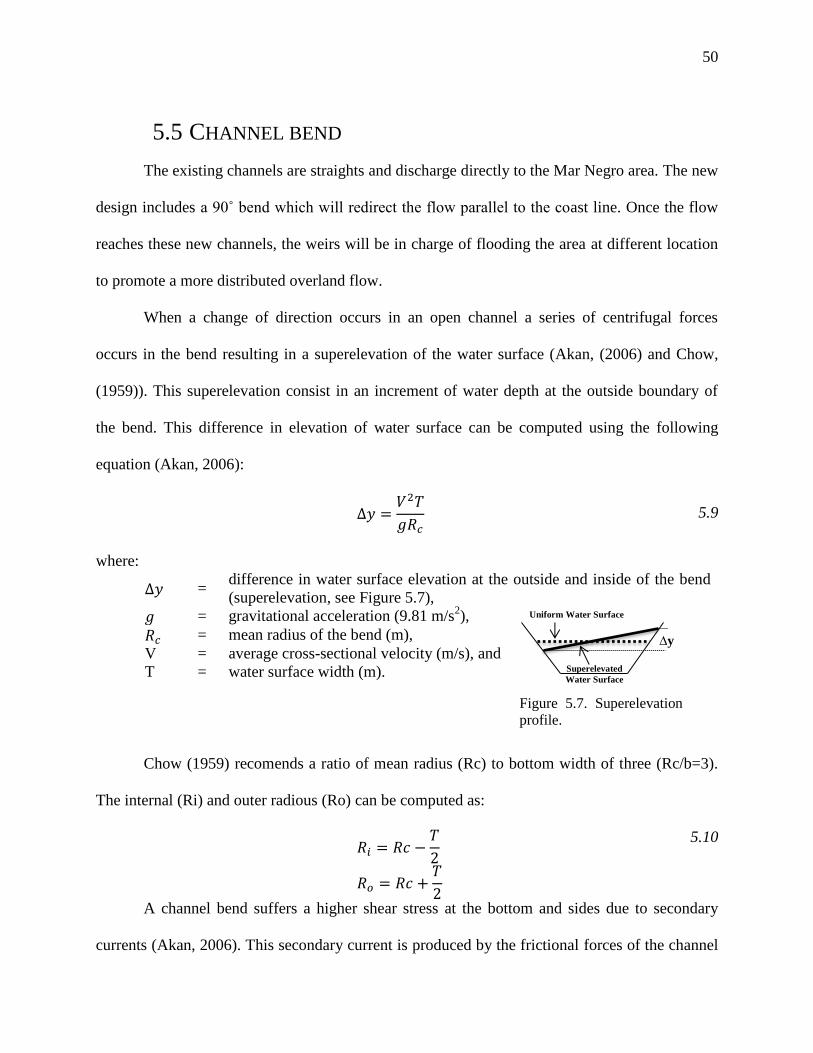
50
The existing channels are straights and discharge directly to the Mar Negro area. The new
design includes a 90˚ bend which will redirect the flow parallel to the coast line. Once the flow
reaches these new channels, the weirs will be in charge of flooding the area at different location
to promote a more distributed overland flow.
When a change of direction occurs in an open channel a series of centrifugal forces
occurs in the bend resulting in a superelevation of the water surface (Akan, (2006) and Chow,
(1959)). This superelevation consist in an increment of water depth at the outside boundary of
the bend. This difference in elevation of water surface can be computed using the following
equation (Akan, 2006):
5.9
where:
= difference in water surface elevation at the outside and inside of the bend
(superelevation, see Figure 5.7),
= gravitational acceleration (9.81 m/s2),
= mean radius of the bend (m),
V = average cross-sectional velocity (m/s), and
T = water surface width (m).
Chow (1959) recomends a ratio of mean radius (Rc) to bottom width of three (Rc/b=3).
The internal (Ri) and outer radious (Ro) can be computed as:
5.10
A channel bend suffers a higher shear stress at the bottom and sides due to secondary
currents (Akan, 2006). This secondary current is produced by the frictional forces of the channel
5.5 CHANNEL BEND
Uniform Water Surface
Superelevated
Water Surface
∆y
Figure 5.7. Superelevation
profile.
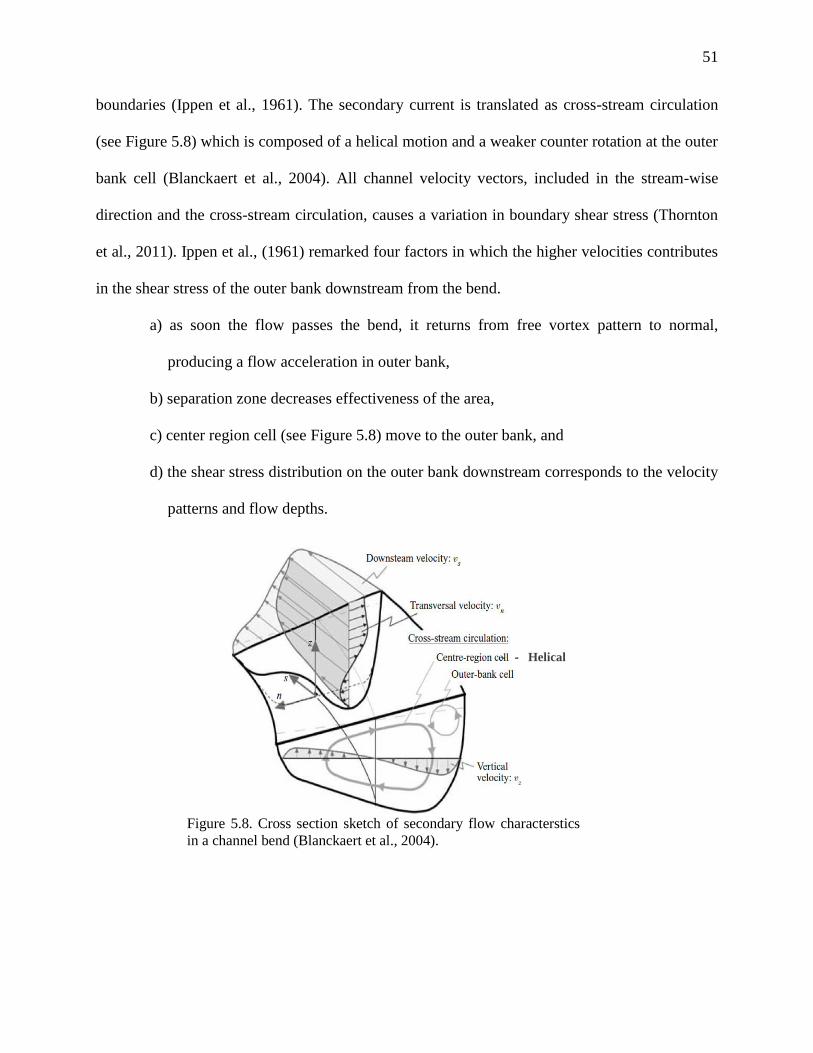
51
boundaries (Ippen et al., 1961). The secondary current is translated as cross-stream circulation
(see Figure 5.8) which is composed of a helical motion and a weaker counter rotation at the outer
bank cell (Blanckaert et al., 2004). All channel velocity vectors, included in the stream-wise
direction and the cross-stream circulation, causes a variation in boundary shear stress (Thornton
et al., 2011). Ippen et al., (1961) remarked four factors in which the higher velocities contributes
in the shear stress of the outer bank downstream from the bend.
a) as soon the flow passes the bend, it returns from free vortex pattern to normal,
producing a flow acceleration in outer bank,
b) separation zone decreases effectiveness of the area,
c) center region cell (see Figure 5.8) move to the outer bank, and
d) the shear stress distribution on the outer bank downstream corresponds to the velocity
patterns and flow depths.
Figure 5.8. Cross section sketch of secondary flow characterstics
in a channel bend (Blanckaert et al., 2004).
- - Helical
52
A minimum protection length is necesarry to prevent a geometrical erosion after the
channel bend. The protection length can be computed as follows (Akan, 2006):
⁄
5.11
where:
= protection length (m),
= 0.736 m -1/6
,
= Manning roughness coefficient, and
R = hydraulic radius (m).
Strictly speaking, lined channel should be able to resist increased shear stress due to
bends geometry. The length used in this design was 13.5 m, which exceeds the length
recommended by the equation 5.11 (see Table 5.3). Figure 5.9 shows the shear stress zones
produced by the flow in the channel bend and the protection length that must be used to prevent
erosion in the channel. The increase on shear stress on the bend will depend on the critical shear
stress allowed by the channel lining. If the shear stress caused by the channel bend is higher than
the critical shear stress, the channel lining must be changed in order to complete an effective
design. The increase of shear stress in the channel will be dictated by a coefficient Kbend which
can be found using Figure 5.9 with the Rc/b. The Rc/b is the ratio of the radius at the center by
the bottom width of the channel.
This shear stress on the bottom and the sidewalls caused by the channel bend can be
calculated using the following equations:
5.12
and
5.13

53
where:
= side shear stress at channel bend,
= side shear stress for straight channel (Table 5.3),
= dimensionless coefficient obtained in Figure 5.9,
= bottom shear stress at channel bend, and
= bottom shear stress.
The superelevation for both channels is less than five centimeters which means that can
be ignored. The dimensionless coefficient obtained, using a Rc/b ratio of three (3), is 1.86. If
and are lower than the critical shear stress calculated in the riprap design (see Table 5.3) the
curve will satisfy the design and no further changes has to be done to complete this part of the
channel design. This condition is satisfied in this case.
Figure 5.9. A: Channel diagram. B: Dimensionless coefficient for shear stress caused by channel bends
calculation (Akan, 2006).
Lp = Protection Length (m)
P.C. = Point on curve
P.T. = Point on tangent
RC = Radius of channel center line. (m)
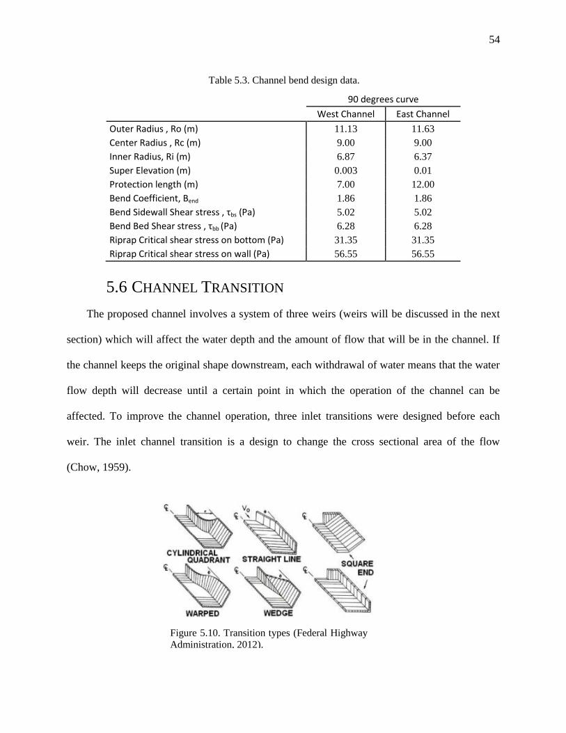
54
90 degrees curve
West Channel East Channel
Outer Radius , Ro (m) 11.13 11.63
Center Radius , Rc (m) 9.00 9.00
Inner Radius, Ri (m) 6.87 6.37
Super Elevation (m) 0.003 0.01
Protection length (m) 7.00 12.00
Bend Coefficient, Bend 1.86 1.86
Bend Sidewall Shear stress , τbs (Pa) 5.02 5.02
Bend Bed Shear stress , τbb (Pa) 6.28 6.28
Riprap Critical shear stress on bottom (Pa) 31.35 31.35
Riprap Critical shear stress on wall (Pa) 56.55 56.55
The proposed channel involves a system of three weirs (weirs will be discussed in the next
section) which will affect the water depth and the amount of flow that will be in the channel. If
the channel keeps the original shape downstream, each withdrawal of water means that the water
flow depth will decrease until a certain point in which the operation of the channel can be
affected. To improve the channel operation, three inlet transitions were designed before each
weir. The inlet channel transition is a design to change the cross sectional area of the flow
(Chow, 1959).
5.6 CHANNEL TRANSITION
Figure 5.10. Transition types (Federal Highway
Administration, 2012).
Table 5.3. Channel bend design data.
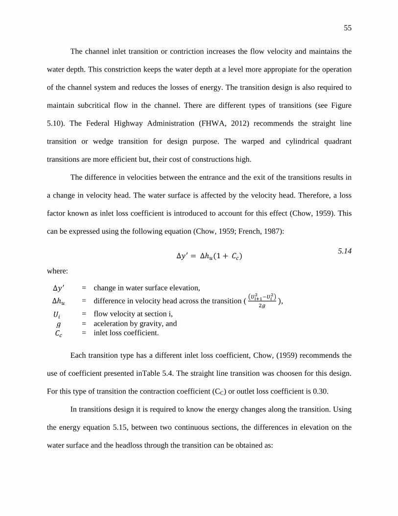
55
The channel inlet transition or contriction increases the flow velocity and maintains the
water depth. This constriction keeps the water depth at a level more appropiate for the operation
of the channel system and reduces the losses of energy. The transition design is also required to
maintain subcritical flow in the channel. There are different types of transitions (see Figure
5.10). The Federal Highway Administration (FHWA, 2012) recommends the straight line
transition or wedge transition for design purpose. The warped and cylindrical quadrant
transitions are more efficient but, their cost of constructions high.
The difference in velocities between the entrance and the exit of the transitions results in
a change in velocity head. The water surface is affected by the velocity head. Therefore, a loss
factor known as inlet loss coefficient is introduced to account for this effect (Chow, 1959). This
can be expressed using the following equation (Chow, 1959; French, 1987):
5.14
where:
= change in water surface elevation,
= difference in velocity head across the transition ( (
)
,
= flow velocity at section i,
= aceleration by gravity, and
= inlet loss coefficient.
Each transition type has a different inlet loss coefficient, Chow, (1959) recommends the
use of coefficient presented inTable 5.4. The straight line transition was choosen for this design.
For this type of transition the contraction coefficient (CC) or outlet loss coefficient is 0.30.
In transitions design it is required to know the energy changes along the transition. Using
the energy equation 5.15, between two continuous sections, the differences in elevation on the
water surface and the headloss through the transition can be obtained as:
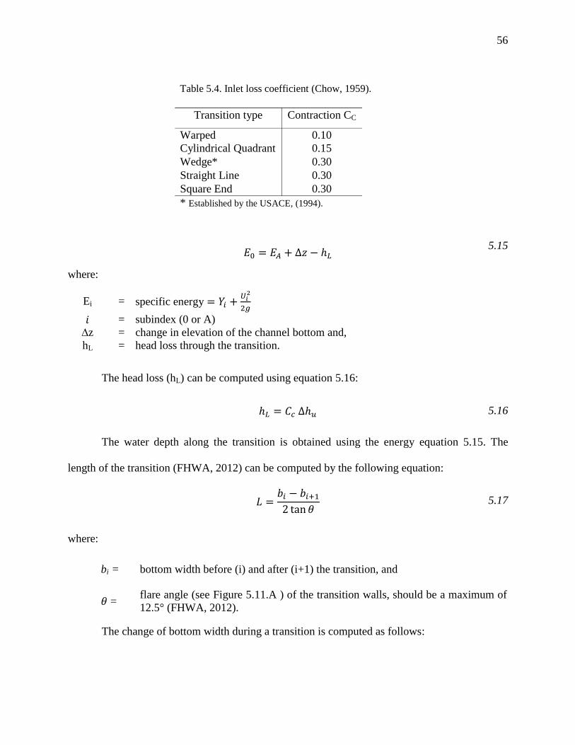
56
5.15
where:
The head loss (hL) can be computed using equation 5.16:
The water depth along the transition is obtained using the energy equation 5.15. The
length of the transition (FHWA, 2012) can be computed by the following equation:
5.17
where:
bi = bottom width before (i) and after (i+1) the transition, and
= flare angle (see Figure 5.11.A ) of the transition walls, should be a maximum of
12.5° (FHWA, 2012).
The change of bottom width during a transition is computed as follows:
Ei = specific energy
= subindex (0 or A)
∆z = change in elevation of the channel bottom and,
hL = head loss through the transition.
5.16
Table 5.4. Inlet loss coefficient (Chow, 1959).
Transition type Contraction CC
Warped 0.10
Cylindrical Quadrant 0.15
Wedge* 0.30
Straight Line 0.30
Square End 0.30
* Established by the USACE, (1994).

57
[ (
)
] 5.18
5.19
√ 5.20
where:
Figure 5.11 shows the schematic of the transition and the energy grade line .
The transitions were designed to reduce the bottom width of the channel gradually. This
was achieved by designing three different transitions in which the channel bottom width reduces
from 3 m to 0.5 m. Figure 5.12 shows the steps followed during the design process, which is a
representation an adaptation of the standard step method (Chow, 1959).
The channel design involves gradually variable flow conditions due to the change on
geometry. The computations start downstream and continues in the upstream direction. The
energy equation between two sections is :
5.21
where: z is the elevation from a datum to the channel bottom, U is the average velocity in the
channel, Y is the channel depth, g is acelleration by gravity, and hL and hf total head loss and
friction loss in the channel between the two sections, respectively.
= bottom width at the section,
bi = bottom width upstream,
bi+1 = bottom width downstream,.
L = computed transition length (see equation 5.19),
x = variation in transition length, 0 ≥ x ≥ L,
TL = length rounded up to the nearest whole number,
m = channel side slope, and
Y = channel depth.
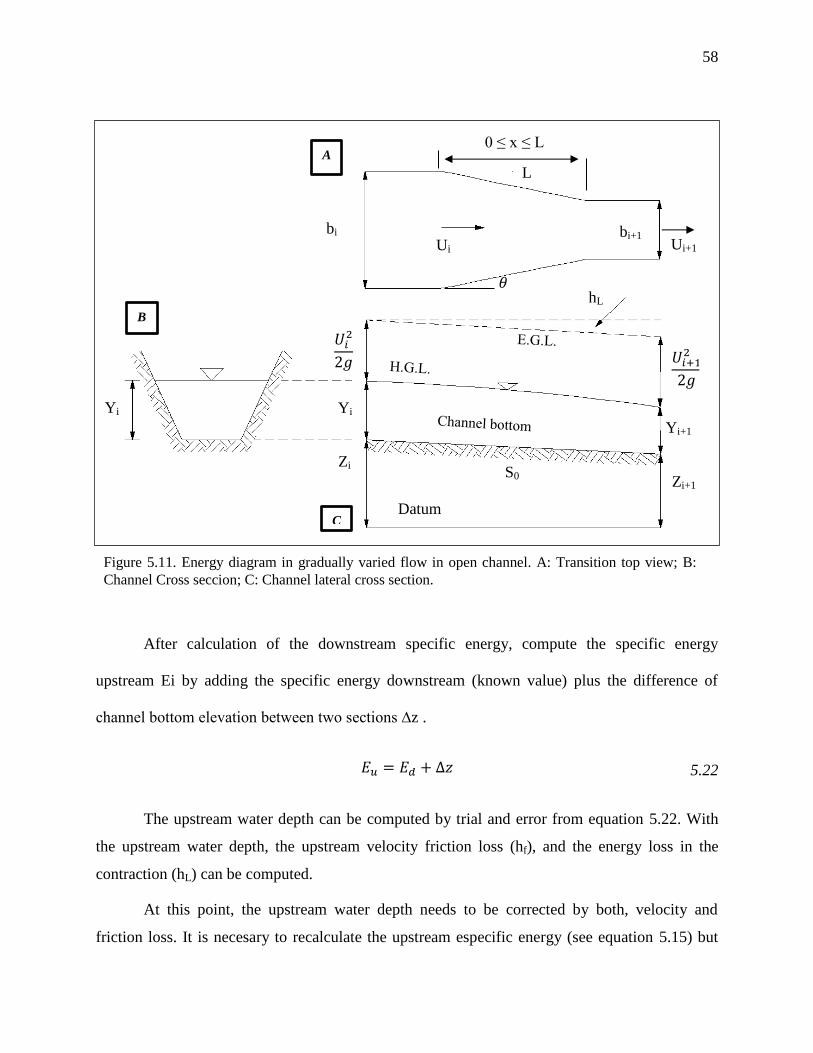
58
Figure 5.11. Energy diagram in gradually varied flow in open channel. A: Transition top view; B:
Channel Cross seccion; C: Channel lateral cross section.
Z2
Zi
Yi
𝑈𝑖
𝑔
Yi+1
hL
𝑈𝑖
𝑔
Datum
S0
Zi+1
bi Ui
bi+1 Ui+1
L
𝜃
A
C
B
0 ≤ x ≤ L
Yi
After calculation of the downstream specific energy, compute the specific energy
upstream Ei by adding the specific energy downstream (known value) plus the difference of
channel bottom elevation between two sections ∆z .
The upstream water depth can be computed by trial and error from equation 5.22. With
the upstream water depth, the upstream velocity friction loss (hf), and the energy loss in the
contraction (hL) can be computed.
At this point, the upstream water depth needs to be corrected by both, velocity and
friction loss. It is necesary to recalculate the upstream especific energy (see equation 5.15) but
5.22
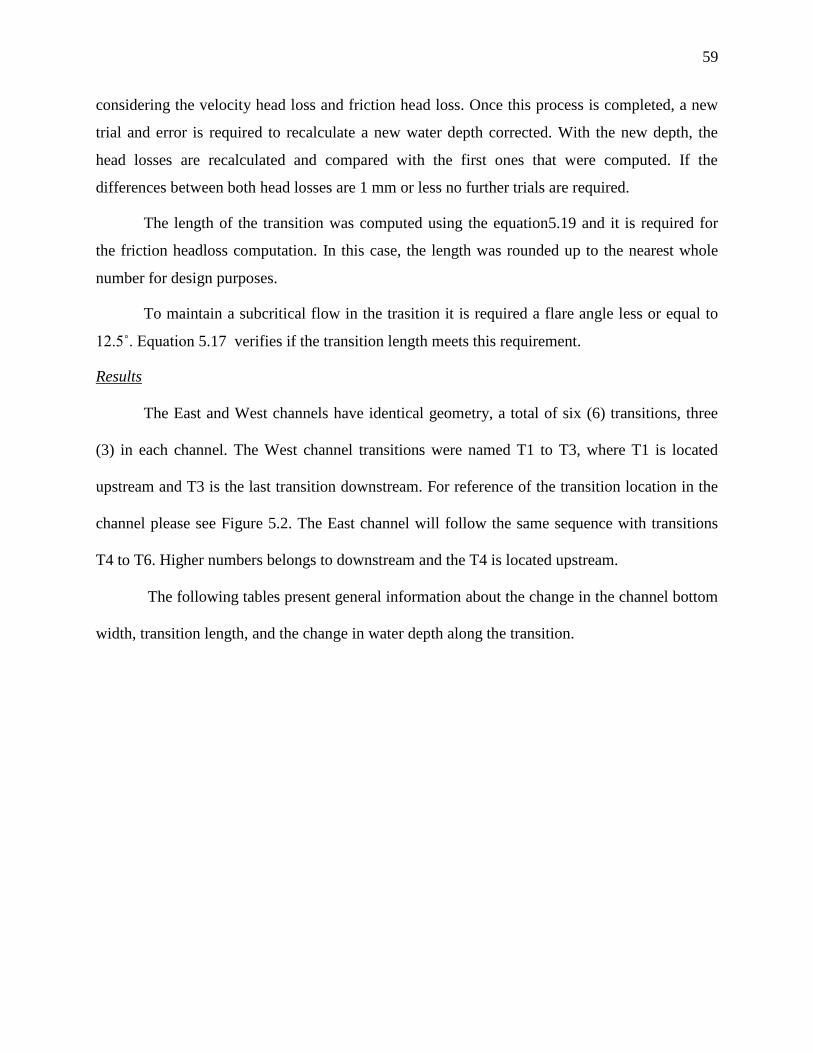
59
considering the velocity head loss and friction head loss. Once this process is completed, a new
trial and error is required to recalculate a new water depth corrected. With the new depth, the
head losses are recalculated and compared with the first ones that were computed. If the
differences between both head losses are 1 mm or less no further trials are required.
The length of the transition was computed using the equation5.19 and it is required for
the friction headloss computation. In this case, the length was rounded up to the nearest whole
number for design purposes.
To maintain a subcritical flow in the trasition it is required a flare angle less or equal to
12.5˚. Equation 5.17 verifies if the transition length meets this requirement.
Results
The East and West channels have identical geometry, a total of six (6) transitions, three
(3) in each channel. The West channel transitions were named T1 to T3, where T1 is located
upstream and T3 is the last transition downstream. For reference of the transition location in the
channel please see Figure 5.2. The East channel will follow the same sequence with transitions
T4 to T6. Higher numbers belongs to downstream and the T4 is located upstream.
The following tables present general information about the change in the channel bottom
width, transition length, and the change in water depth along the transition.
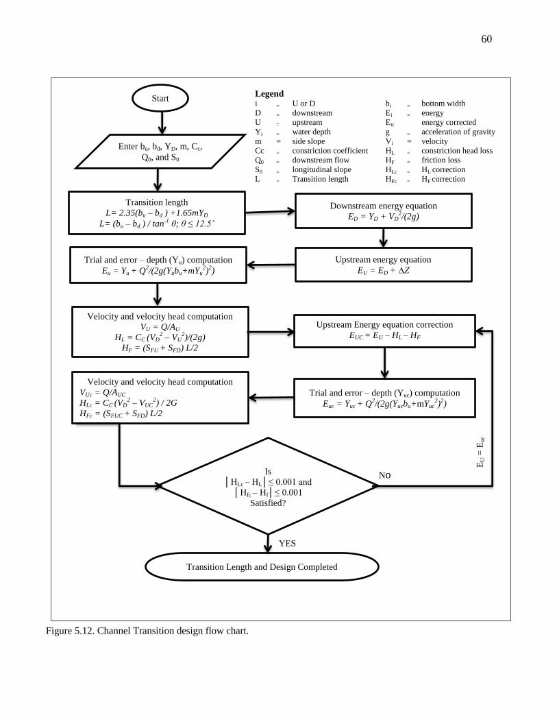
60
EU =
Euc
Upstream Energy equation correction
EUC = EU – HL – HF
Trial and error – depth (Yuc) computation
Euc = Yuc + Q2/(2g(Yucbu+mYuc
2)2)
Downstream energy equation
ED = YD + VD2/(2g)
Upstream energy equation
EU = ED + ∆Z
Trial and error – depth (Yu) computation
Eu = Yu + Q2/(2g(Yubu+mYu
2)
2)
Start
Enter bu, bd, YD, m, Cc,
Q0, and S0
Transition length
L= 2.35(bu – bd ) +1.65mYD
L= (bu – bd ) / tan-1
θ; θ ≤ 12.5˚
Velocity and velocity head computation
VU = Q/AU
HL = CC (VD2 – VU
2)/(2g)
HF = (SFU + SFD) L/2
Velocity and velocity head computation
VUc = Q/AUC
HLc = CC (VD2 – VUC
2) / 2G
HFc = (SFUC + SFD) L/2
Is
│HLc – HL│≤ 0.001 and
│Hfc – Hf│≤ 0.001
Satisfied?
Transition Length and Design Completed
No
YES
Figure 5.12. Channel Transition design flow chart.
Legend i = U or D
D = downstream
U = upstream
Yi = water depth m = side slope
Cc = constriction coefficient
Q0 = downstream flow
S0 = longitudinal slope
L = Transition length
bi = bottom width Ei = energy
Eic energy corrected
g = acceleration of gravity
Vi = velocity
HL = constriction head loss
HF = friction loss
HLc = HL correction
HFc = HF correction
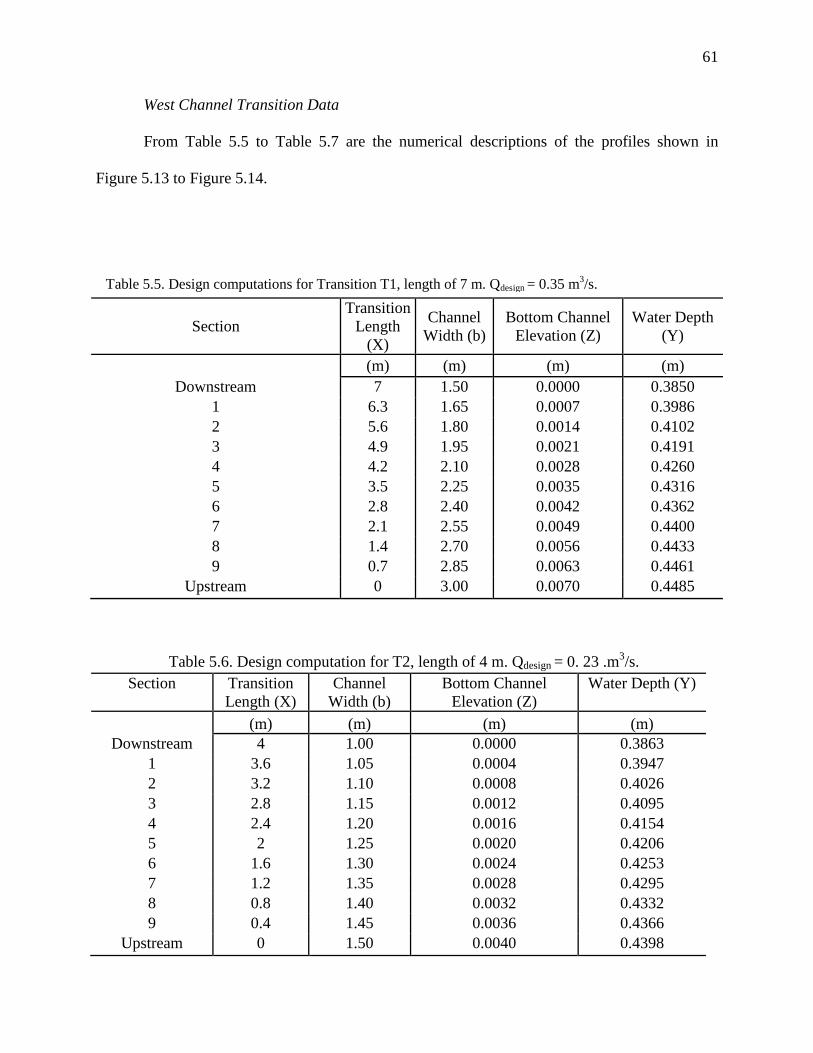
61
West Channel Transition Data
From Table 5.5 to Table 5.7 are the numerical descriptions of the profiles shown in
Figure 5.13 to Figure 5.14.
Section
Transition
Length
(X)
Channel
Width (b)
Bottom Channel
Elevation (Z)
Water Depth
(Y)
(m) (m) (m) (m)
Downstream 7 1.50 0.0000 0.3850
1 6.3 1.65 0.0007 0.3986
2 5.6 1.80 0.0014 0.4102
3 4.9 1.95 0.0021 0.4191
4 4.2 2.10 0.0028 0.4260
5 3.5 2.25 0.0035 0.4316
6 2.8 2.40 0.0042 0.4362
7 2.1 2.55 0.0049 0.4400
8 1.4 2.70 0.0056 0.4433
9 0.7 2.85 0.0063 0.4461
Upstream 0 3.00 0.0070 0.4485
Section Transition
Length (X)
Channel
Width (b)
Bottom Channel
Elevation (Z)
Water Depth (Y)
(m) (m) (m) (m)
Downstream 4 1.00 0.0000 0.3863
1 3.6 1.05 0.0004 0.3947
2 3.2 1.10 0.0008 0.4026
3 2.8 1.15 0.0012 0.4095
4 2.4 1.20 0.0016 0.4154
5 2 1.25 0.0020 0.4206
6 1.6 1.30 0.0024 0.4253
7 1.2 1.35 0.0028 0.4295
8 0.8 1.40 0.0032 0.4332
9 0.4 1.45 0.0036 0.4366
Upstream 0 1.50 0.0040 0.4398
Qdesign = 0. 23 .m3/s.Table 5.6. Design computation for T2, length of 4 m.
Table 5.5. Design computations for Transition T1, length of 7 m. Qdesign = 0.35 m3/s.
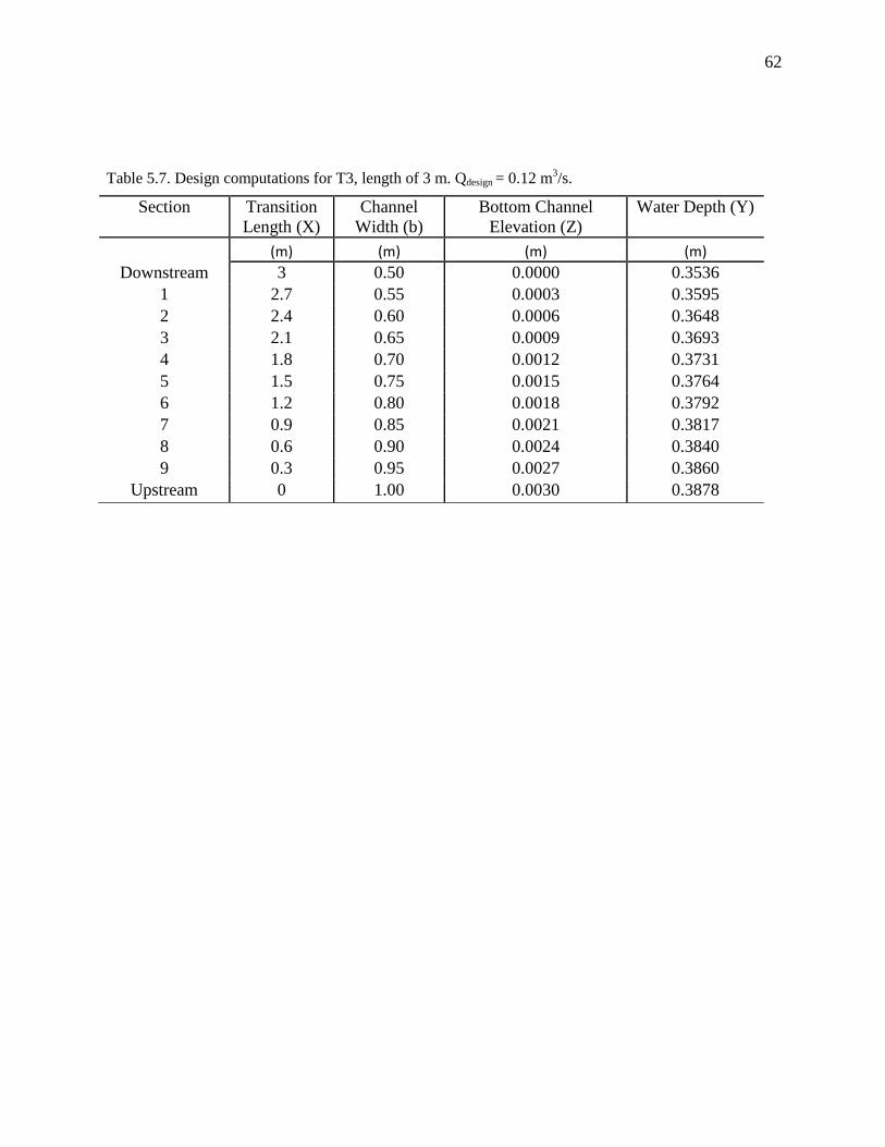
62
Section Transition
Length (X) Channel
Width (b) Bottom Channel
Elevation (Z) Water Depth (Y)
(m) (m) (m) (m)
Downstream 3 0.50 0.0000 0.3536
1 2.7 0.55 0.0003 0.3595
2 2.4 0.60 0.0006 0.3648
3 2.1 0.65 0.0009 0.3693
4 1.8 0.70 0.0012 0.3731
5 1.5 0.75 0.0015 0.3764
6 1.2 0.80 0.0018 0.3792
7 0.9 0.85 0.0021 0.3817
8 0.6 0.90 0.0024 0.3840
9 0.3 0.95 0.0027 0.3860
Upstream 0 1.00 0.0030 0.3878
Table 5.7. Design computations for T3, length of 3 m. Qdesign = 0.12 m3/s.
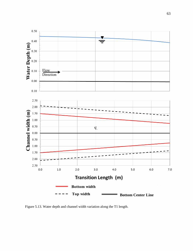
63
Figure 5.13. Water depth and channel width variation along the T1 length.
Bottom Center Line
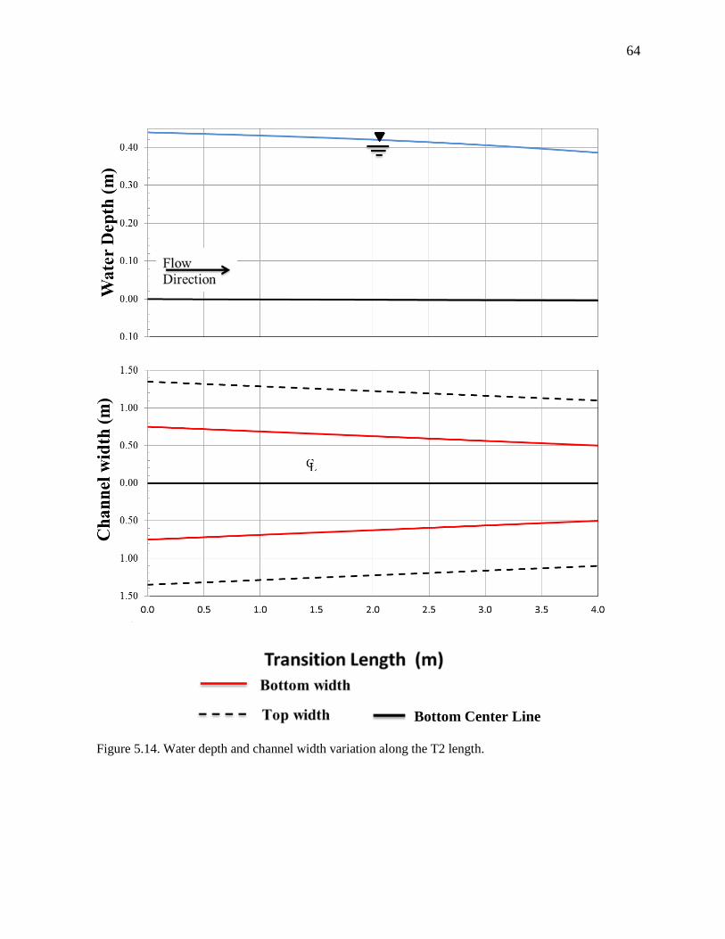
64
Figure 5.14. Water depth and channel width variation along the T2 length.
Bottom Center Line
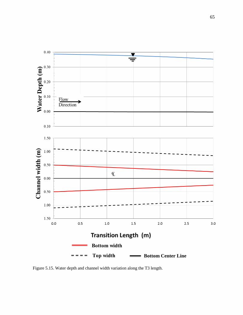
65
Figure 5.15. Water depth and channel width variation along the T3 length.
Bottom Center Line
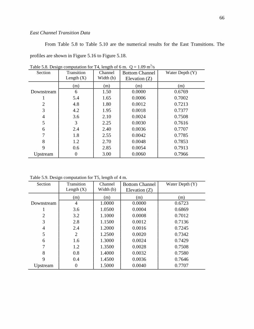
66
East Channel Transition Data
From Table 5.8 to Table 5.10 are the numerical results for the East Transitions. The
profiles are shown in Figure 5.16 to Figure 5.18.
Table 5.8. Design computation for T4, length of 6 m. Q = 1.09 m3/s
Section Transition
Length (X)
Channel
Width (b) Bottom Channel
Elevation (Z)
Water Depth (Y)
(m) (m) (m) (m)
Downstream 6 1.50 0.0000 0.6769
1 5.4 1.65 0.0006 0.7002
2 4.8 1.80 0.0012 0.7213
3 4.2 1.95 0.0018 0.7377
4 3.6 2.10 0.0024 0.7508
5 3 2.25 0.0030 0.7616
6 2.4 2.40 0.0036 0.7707
7 1.8 2.55 0.0042 0.7785
8 1.2 2.70 0.0048 0.7853
9 0.6 2.85 0.0054 0.7913
Upstream 0 3.00 0.0060 0.7966
Table 5.9. Design computation for T5, length of 4 m.
Section Transition
Length (X)
Channel
Width (b) Bottom Channel
Elevation (Z)
Water Depth (Y)
(m) (m) (m) (m)
Downstream 4 1.0000 0.0000 0.6723
1 3.6 1.0500 0.0004 0.6869
2 3.2 1.1000 0.0008 0.7012
3 2.8 1.1500 0.0012 0.7136
4 2.4 1.2000 0.0016 0.7245
5 2 1.2500 0.0020 0.7342
6 1.6 1.3000 0.0024 0.7429
7 1.2 1.3500 0.0028 0.7508
8 0.8 1.4000 0.0032 0.7580
9 0.4 1.4500 0.0036 0.7646
Upstream 0 1.5000 0.0040 0.7707
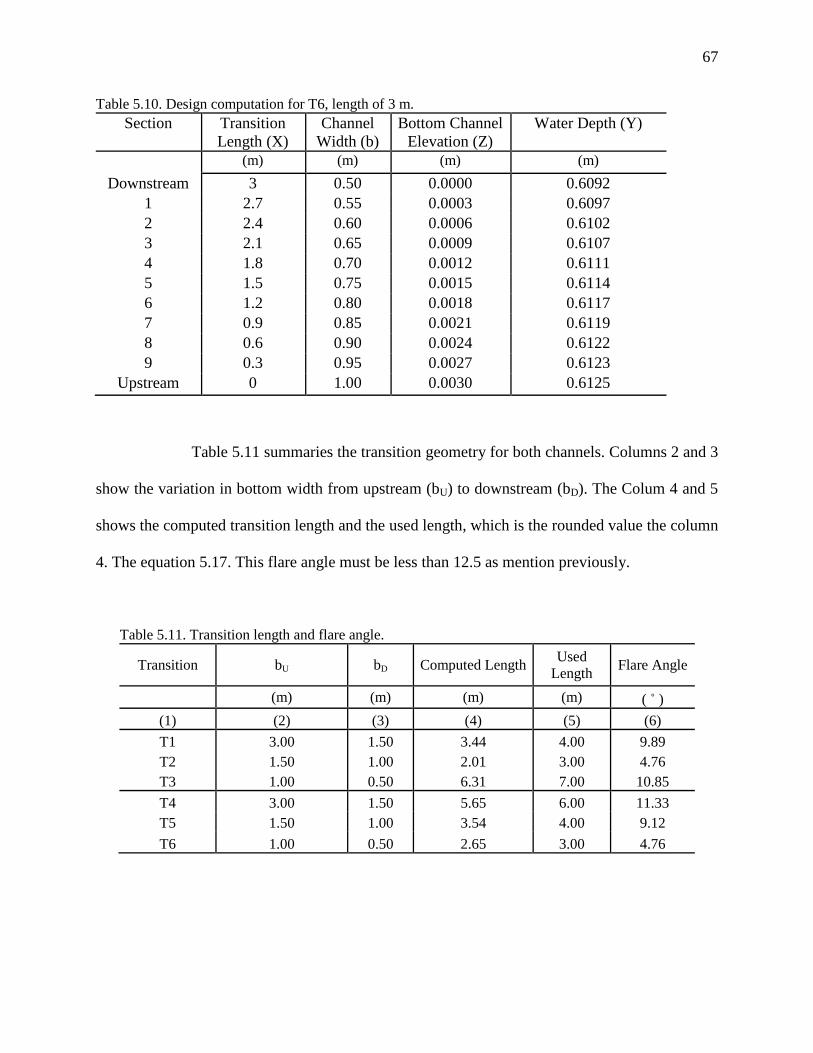
67
Table 5.10. Design computation for T6, length of 3 m.
Table 5.11 summaries the transition geometry for both channels. Columns 2 and 3
show the variation in bottom width from upstream (bU) to downstream (bD). The Colum 4 and 5
shows the computed transition length and the used length, which is the rounded value the column
4. The equation 5.17. This flare angle must be less than 12.5 as mention previously.
Table 5.11. Transition length and flare angle.
Transition bU bD Computed Length Used
Length Flare Angle
(m) (m) (m) (m) ( ˚ )
(1) (2) (3) (4) (5) (6)
T1 3.00 1.50 3.44 4.00 9.89
T2 1.50 1.00 2.01 3.00 4.76
T3 1.00 0.50 6.31 7.00 10.85
T4 3.00 1.50 5.65 6.00 11.33
T5 1.50 1.00 3.54 4.00 9.12
T6 1.00 0.50 2.65 3.00 4.76
Section Transition
Length (X) Channel
Width (b) Bottom Channel
Elevation (Z) Water Depth (Y)
(m) (m) (m) (m)
Downstream 3 0.50 0.0000 0.6092
1 2.7 0.55 0.0003 0.6097
2 2.4 0.60 0.0006 0.6102
3 2.1 0.65 0.0009 0.6107
4 1.8 0.70 0.0012 0.6111
5 1.5 0.75 0.0015 0.6114
6 1.2 0.80 0.0018 0.6117
7 0.9 0.85 0.0021 0.6119
8 0.6 0.90 0.0024 0.6122
9 0.3 0.95 0.0027 0.6123
Upstream 0 1.00 0.0030 0.6125
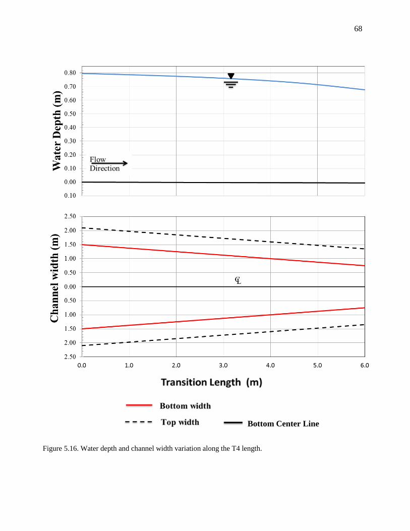
68
Figure 5.16. Water depth and channel width variation along the T4 length.
Bottom Center Line
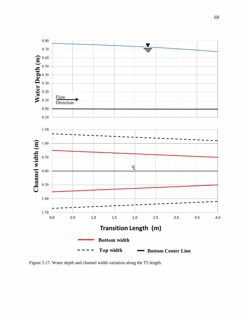
69
Figure 5.17. Water depth and channel width variation along the T5 length.
Bottom Center Line
Center Line
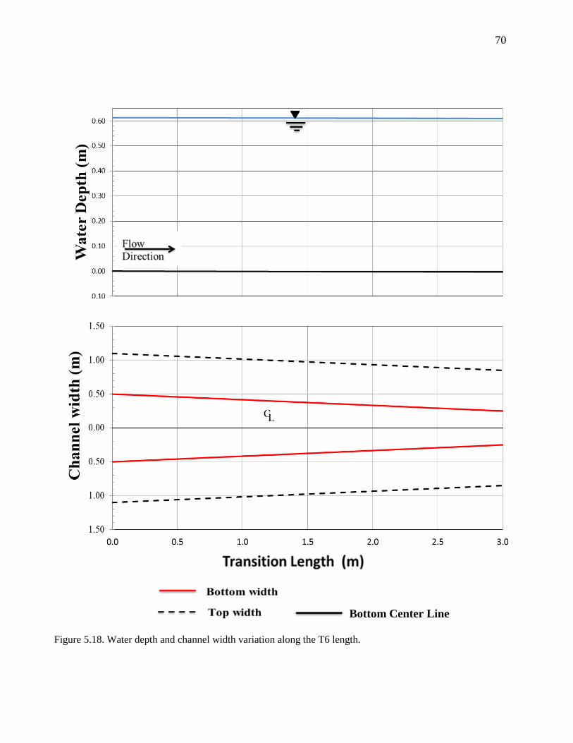
70
Figure 5.18. Water depth and channel width variation along the T6 length.
Bottom Center Line
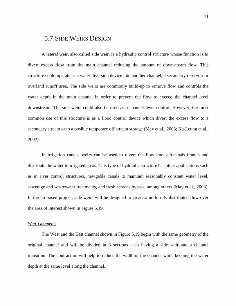
71
A lateral weir, also called side weir, is a hydraulic control structure whose function is to
divert excess flow from the main channel reducing the amount of downstream flow. This
structure could operate as a water diversion device into another channel, a secondary reservoir or
overland runoff area. The side weirs are commonly build-up to remove flow and controls the
water depth in the main channel in order to prevent the flow to exceed the channel level
downstream. The side weirs could also be used as a channel level control. However, the most
common use of this structure is as a flood control device which divert the excess flow to a
secondary stream or to a posible temporary off stream storage (May et al., 2003; Ka-Leung et al.,
2002).
In irrigation canals, weirs can be used to divert the flow into sub-canals branch and
distribute the water to irrigated areas. This type of hydraulic structure has other applications such
as in river control structures, navigable canals to maintain reasonably constant water level,
sewerage and wastewater treatments, and trash screens bypass, among others (May et al., 2003).
In the proposed project, side weirs will be designed to create a uniformly distributed flow over
the area of interest shown in Figure 5.19.
Weir Geometry
The West and the East channel shown in Figure 5.19 begin with the same geometry of the
original channel and will be divided in 3 sections each having a side weir and a channel
transition. The contraction will help to reduce the width of the channel while keeping the water
depth at the same level along the channel.
5.7 SIDE WEIRS DESIGN
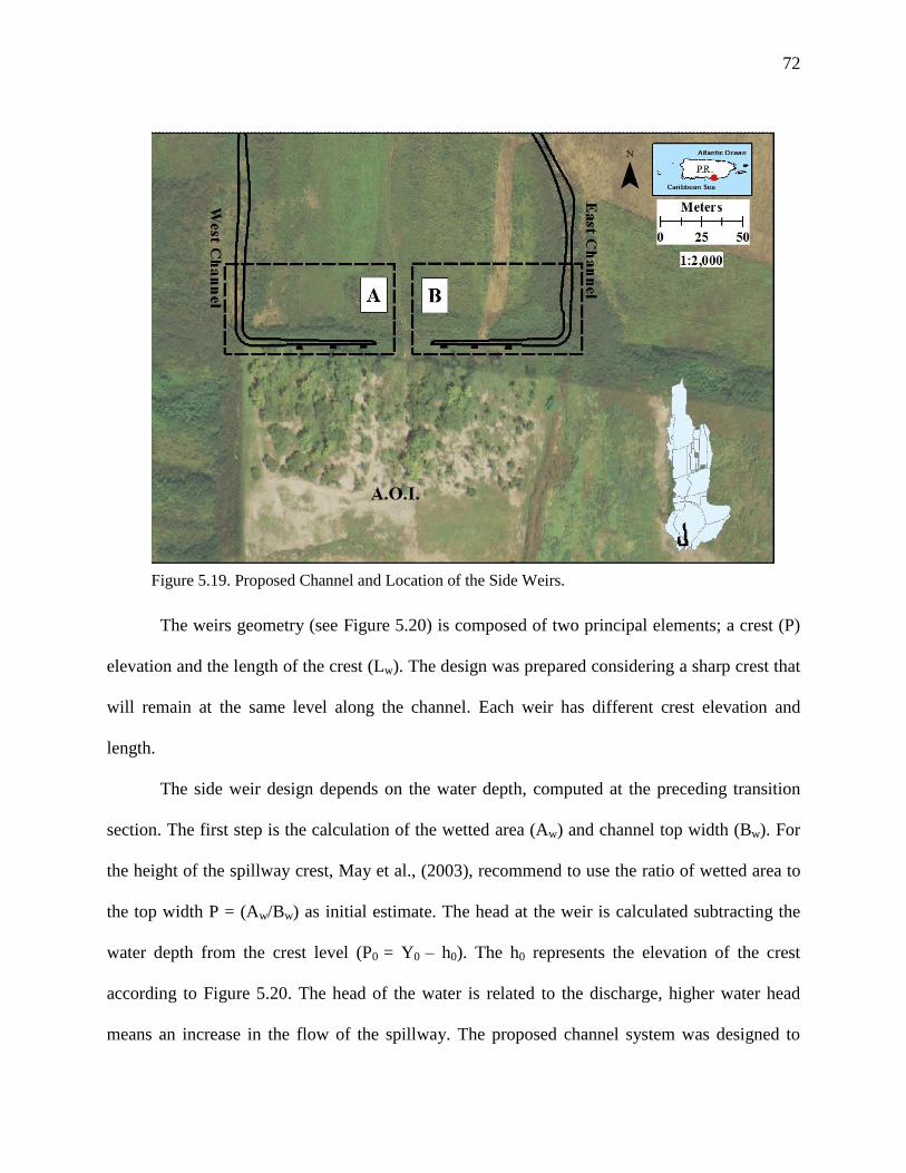
72
The weirs geometry (see Figure 5.20) is composed of two principal elements; a crest (P)
elevation and the length of the crest (Lw). The design was prepared considering a sharp crest that
will remain at the same level along the channel. Each weir has different crest elevation and
length.
The side weir design depends on the water depth, computed at the preceding transition
section. The first step is the calculation of the wetted area (Aw) and channel top width (Bw). For
the height of the spillway crest, May et al., (2003), recommend to use the ratio of wetted area to
the top width P = (Aw/Bw) as initial estimate. The head at the weir is calculated subtracting the
water depth from the crest level (P0 = Y0 – h0). The h0 represents the elevation of the crest
according to Figure 5.20. The head of the water is related to the discharge, higher water head
means an increase in the flow of the spillway. The proposed channel system was designed to
Figure 5.19. Proposed Channel and Location of the Side Weirs.
(b)
73
discharge approximately the same amount of water over each of the first two (2) weirs and the
remaining flow in the last.
Froude Number
The Froude number is a non-dimensional parameter which helps to determine the flow
conditions upstream and downstream of the side weir. Froude number can have a direct influence
on the operation of the weir flow. When the value of this parameter is equal to one the flow is
considered critical. If the value is greater than one, the flow is considered fast or supercritical.
Furthermore, if the value is less than one, it implies a slow or tranquil flow, called subcritical
flow.
The Froude number is calculated using the following equation:
where:
Q = Discharge (m3/s),
= Area (m2),
= acceleration by gravity (9.81 m/s2), and
=
hydraulic depth (m) .
√ 5.23
YY0
Figure 5.20. Typical operation of side weir: A: Water depth across the side weir. B:
Top view of the side weir (May et al., 2003).
QA
A
B
Bw
P0
QS
QO QA
h0
Lw
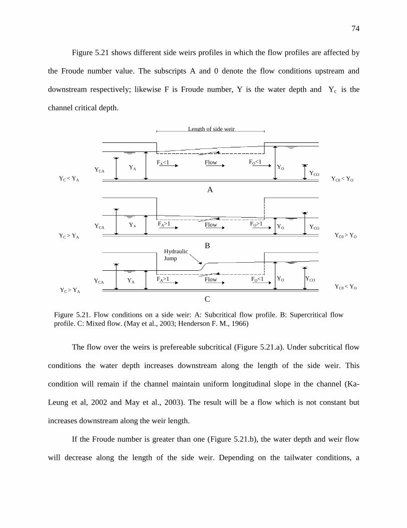
74
Figure 5.21 shows different side weirs profiles in which the flow profiles are affected by
the Froude number value. The subscripts A and 0 denote the flow conditions upstream and
downstream respectively; likewise F is Froude number, Y is the water depth and Yc is the
channel critical depth.
The flow over the weirs is prefereable subcritical (Figure 5.21.a). Under subcritical flow
conditions the water depth increases downstream along the length of the side weir. This
condition will remain if the channel maintain uniform longitudinal slope in the channel (Ka-
Leung et al, 2002 and May et al., 2003). The result will be a flow which is not constant but
increases downstream along the weir length.
If the Froude number is greater than one (Figure 5.21.b), the water depth and weir flow
will decrease along the length of the side weir. Depending on the tailwater conditions, a
YC0 < YO
YC > YA YC0 > YO
YC > YA YC0 < YO
Figure 5.21. Flow conditions on a side weir: A: Subcritical flow profile. B: Supercritical flow
profile. C: Mixed flow. (May et al., 2003; Henderson F. M., 1966)
Flow
Length of side weir
YCA YA
FA<1 FO<1
YCO
YO
FA>1
(a)
(b)
(c)
YA YCA
YCA YA
Flow
Flow
YO YCO
YO YCO FO<1
FO>1
FA>1
Hydraulic
Jump
YC < YA
C
B
A
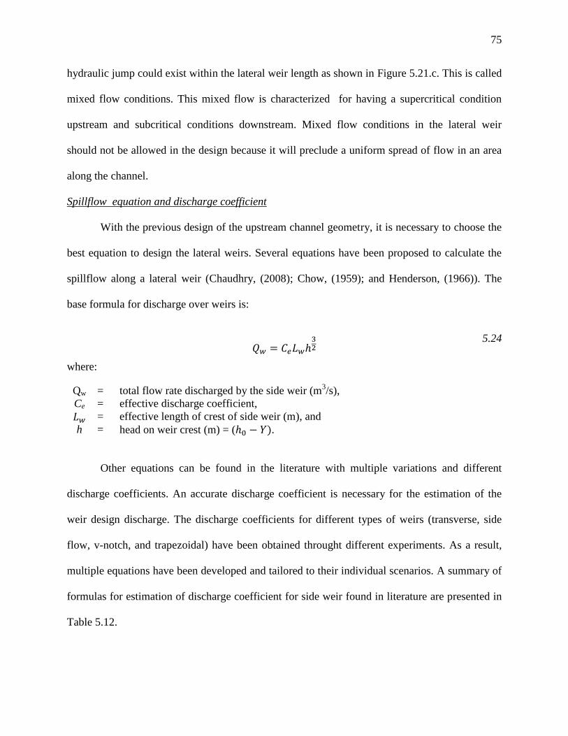
75
hydraulic jump could exist within the lateral weir length as shown in Figure 5.21.c. This is called
mixed flow conditions. This mixed flow is characterized for having a supercritical condition
upstream and subcritical conditions downstream. Mixed flow conditions in the lateral weir
should not be allowed in the design because it will preclude a uniform spread of flow in an area
along the channel.
Spillflow equation and discharge coefficient
With the previous design of the upstream channel geometry, it is necessary to choose the
best equation to design the lateral weirs. Several equations have been proposed to calculate the
spillflow along a lateral weir (Chaudhry, (2008); Chow, (1959); and Henderson, (1966)). The
base formula for discharge over weirs is:
where:
Qw = total flow rate discharged by the side weir (m3/s),
Ce = effective discharge coefficient,
= effective length of crest of side weir (m), and
h = head on weir crest (m) = ( .
Other equations can be found in the literature with multiple variations and different
discharge coefficients. An accurate discharge coefficient is necessary for the estimation of the
weir design discharge. The discharge coefficients for different types of weirs (transverse, side
flow, v-notch, and trapezoidal) have been obtained throught different experiments. As a result,
multiple equations have been developed and tailored to their individual scenarios. A summary of
formulas for estimation of discharge coefficient for side weir found in literature are presented in
Table 5.12.
5.24
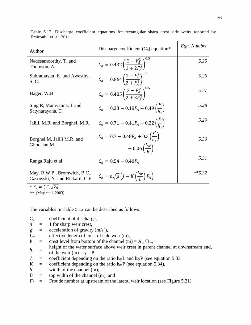
76
Author Discharge coefficient (Cd) equation*
Eqn. Number
Nadesamoorthy, T. and
Thomson, A. (
)
5.25
Subramayan, K. and Awasthy,
S. C. (
)
5.26
Hager, W.H. (
)
5.27
Sing R, Manivanna, T and
Satynarayana, T. (
)
5.28
Jalili, M.R. and Borghei, M.R. (
)
5.29
Borghei M, Jalili M.R. and
Ghodsian M.
(
)
(
)
5.30
Ranga Raju et al. 5.31
May. R.W.P., Bromwich, B.C.,
Gasowski, Y. and Rickard, C.E. √ ( (
) )
**5.32
*
√
** (May et.al, 2003).
The variables in Table 5.12 can be described as follows:
Cu = coefficient of discharge,
n = 1 for sharp weir crest,
= acceleration of gravity (m/s2),
Lw = effective length of crest of side weir (m),
P = crest level from bottom of the channel (m) = Aw /Bw,
h1 = height of the water surface above weir crest in parent channel at downstream end,
of the weir (m) = y – P,
J = coefficient depending on the ratio h0/L and h0/P (see equation 5.33,
K = coefficient depending on the ratio h0/P (see equation 5.34),
b = width of the channel (m),
B = top width of the channel (m), and
FA = Froude number at upstream of the lateral weir location (see Figure 5.21).
Table 5.12. Discharge coefficient equations for rectangular sharp crest side weirs reported by
Emiroglu, et. al, 2011.

77
Coefficients J and K develop by (May, Bromwich, Gasowski, and Rickard, 2003) from
sharp crest weirs data. This coefficients are computed by using the following equation:
where: c1 ans c2 are defined as equation 5.33:
where: is defined as:
and coefficient K is given by:
(
)
5.36
Coefficient K and J were developed by Mays et al. (2003) using data from sharp crested
weirs. Appendix F shows a graphical option to obtain K and J values using the
⁄ ratio.
The discharge coefficient equations, shown in Table 5.12, depend on the following
dimensionless parameters ( Emiroglu et. al, 2011):
(
)
5 .37
where: FA is the upstream Froude number, the side weir length-bottom width ratio which
represents the lateral contraction ratio, the vertical contraction ratio (water head–crest height
ratio) of the side weir, and water head – weir length ratio.
Usually, the change in water depth during the side weir operation is small and can be
ignored. Also the water depth upstream can be approximate as normal depth. For that reason, the
(
(
))
5.33
5.34
⁄
(
⁄ )
5.35

78
Froude number can be calculated using normal depth (Rosier B., 2007). All discharge
coefficients (Cd) were developed for subcritical flows; this means that upstream Froude number
must be less than one. This consideration was used only for the last side weir downstream. The
current project use gradually varied flow computations for the channel design.
The side weirs are structures which produces a reduction of water flow along the length
of the structure. This reduction of water affects the energy as gradient. The energy change during
the operation of this type of structure is a characteristic of a spatially varied flow. The side weirs
design computation will depend on the conservation of mass (Equation 5.38), the conservation of
energy (Equation 5.21) and the Froude number (Equation 5.23) which defines the flow regime.
The continuity equation along the lateral weir is:
5.38
where:
Qin = flow entering to the weir system,
Qspill = spill flow over the weir crest, and
Qout = remainder flow which continues in the system.
Figure 5.22 is a descriptive flowchart of the design procedure. The computation starts
downstream of the last side weir in the channel. Subcritical flow is considered in the design. The
downstream boundary condition depth was assumed as normal depth. The discharge coefficient
was computed with the Equation 5.25 in Table 5.12 of Subramayan, K. and Awasthy, S. C. This
equation is commonly used in the literature (Hager et al., 1986 and Rowlings, 2010) for side
weirs with sharp crest.
5.7.1 SPILLFLOW CALCULATIONS
79
The discharge coefficient is the parameter which controls the amount of flow discharging
over the weir. The SWMM user’s manual (Rossman, 2010) recommends to use for sharp crest
transverse side weirs a constant discharge coefficient (Ce) of 1.84. It is important to mention this
detail because on SWMM the transverse weir replaces the side weir. On the software, the
transverse weirs use equation 5.24 to describe the weir spill flow.
Table 5.13 and Table 5.14 show the discharges coefficients (Cd) from equations in Table 5.12
and the effective discharge coefficient (Ce) computed with the equation
√ . Also
these tables show the calculation of the discharge coefficient using Mays et al. (2003). This
equation represents the value of the effective discharge coefficient. consequenly low coefficients
provide longer weir length and viceversa. Equation 5.26 (equation two in Table 5.3) produces the
maximum discharge coefficient with the weir length less than one meter. The crest height for the
West channel are 0.12, 0.14 and 0.16 m and in the East channel the crest height is 0.20, 0.22, and
0.24 m. All weir crests are at the same elevation from the top of the channel surface.
5.7.2 RESULTS
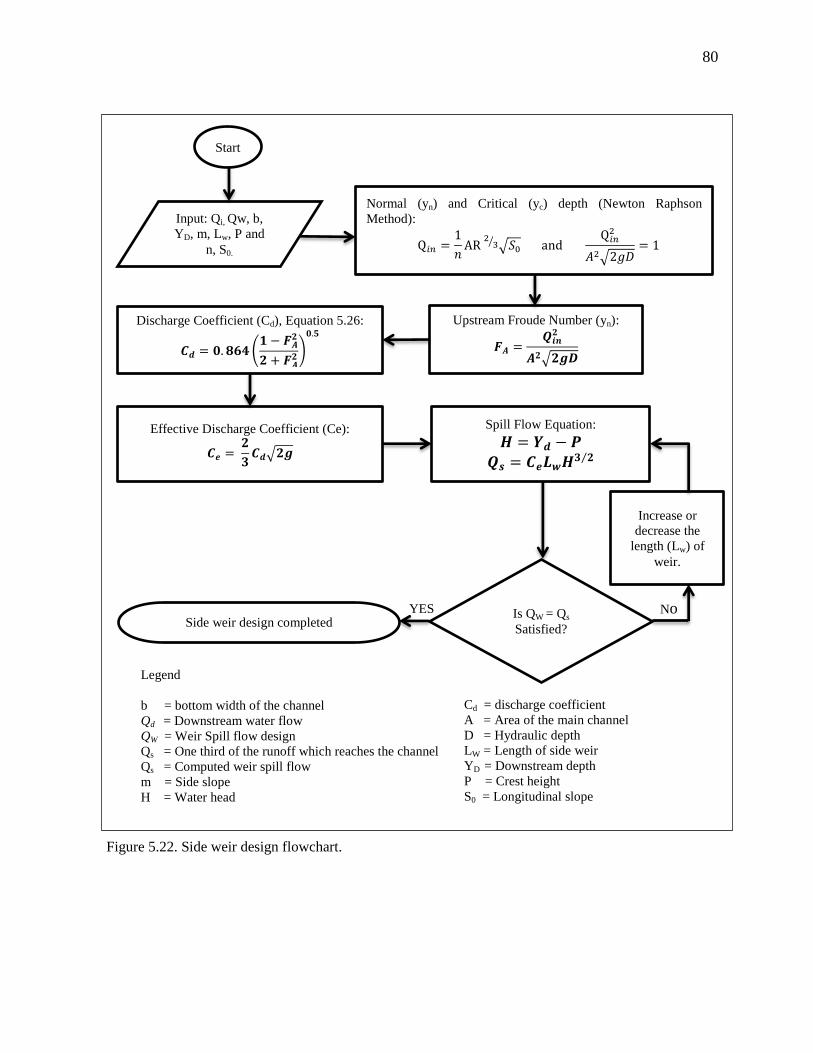
80
Increase or
decrease the
length (Lw) of
weir.
𝑯 𝒀𝒅 𝑷
𝑸𝒔 𝑪𝒆𝑳𝒘𝑯𝟑 𝟐⁄
Spill Flow Equation:
𝑖𝑛
𝑛 R
⁄ √𝑆 d
𝑖𝑛
𝐴 √ 𝑔𝐷
Normal (yn) and Critical (yc) depth (Newton Raphson
Method):
𝑭𝑨 𝑸𝒊𝒏𝟐
𝑨𝟐√𝟐𝒈𝑫
Upstream Froude Number (yn):
𝑪𝒅 𝟎 𝟖𝟔𝟒(𝟏 𝑭𝑨
𝟐
𝟐 𝑭𝑨𝟐)
𝟎 𝟓
Discharge Coefficient (Cd), Equation 5.26:
Start
Input: Qi, Qw, b,
YD, m, Lw, P and
n, S0.
𝑪𝒆 𝟐
𝟑𝑪𝒅√𝟐𝒈
Effective Discharge Coefficient (Ce):
Is QW = Qs
Satisfied? Side weir design completed
YES
Figure 5.22. Side weir design flowchart.
Legend
b = bottom width of the channel
Qd = Downstream water flow
QW = Weir Spill flow design
Qs = One third of the runoff which reaches the channel
Qs = Computed weir spill flow
m = Side slope
H = Water head
No
Cd = discharge coefficient
A = Area of the main channel
D = Hydraulic depth
LW = Length of side weir
YD = Downstream depth
P = Crest height
S0 = Longitudinal slope
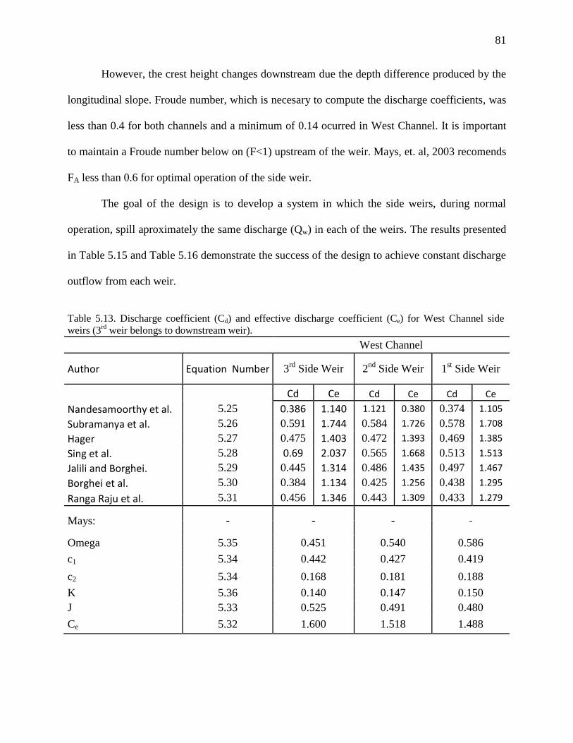
81
However, the crest height changes downstream due the depth difference produced by the
longitudinal slope. Froude number, which is necesary to compute the discharge coefficients, was
less than 0.4 for both channels and a minimum of 0.14 ocurred in West Channel. It is important
to maintain a Froude number below on (F<1) upstream of the weir. Mays, et. al, 2003 recomends
FA less than 0.6 for optimal operation of the side weir.
The goal of the design is to develop a system in which the side weirs, during normal
operation, spill aproximately the same discharge (Qw) in each of the weirs. The results presented
in Table 5.15 and Table 5.16 demonstrate the success of the design to achieve constant discharge
outflow from each weir.
Table 5.13. Discharge coefficient (Cd) and effective discharge coefficient (Ce) for West Channel side
weirs (3rd
weir belongs to downstream weir).
West Channel
Author Equation Number 3rd
Side Weir 2nd
Side Weir 1st Side Weir
Cd Ce Cd Ce Cd Ce
Nandesamoorthy et al. 5.25 0.386 1.140 1.121 0.380 0.374 1.105
Subramanya et al. 5.26 0.591 1.744 0.584 1.726 0.578 1.708
Hager 5.27 0.475 1.403 0.472 1.393 0.469 1.385
Sing et al. 5.28 0.69 2.037 0.565 1.668 0.513 1.513
Jalili and Borghei. 5.29 0.445 1.314 0.486 1.435 0.497 1.467
Borghei et al. 5.30 0.384 1.134 0.425 1.256 0.438 1.295
Ranga Raju et al. 5.31 0.456 1.346 0.443 1.309 0.433 1.279
Mays: - - - -
Omega 5.35 0.451 0.540 0.586
c1 5.34 0.442 0.427 0.419
c2 5.34 0.168 0.181 0.188
K 5.36 0.140 0.147 0.150
J 5.33 0.525 0.491 0.480
Ce 5.32 1.600 1.518 1.488

82
Table 5.14. Discharge coefficient (Cd) and effective discharge coefficient (Ce) for East Channel side
weirs (3rd
weir belongs to downstream).
East Channel
Author Equation Number 3rd
Side Weir 2nd
Side Weir 1st Side Weir
Cd Ce Cd Ce Cd Ce
Nandesamoorthy et al. 5.25 0.383 1.130 0.371 1.095 0.361 1.065
Subramanya et al. 5.26 0.587 1.735 0.575 1.697 0.564 1.665
Hager 5.27 0.449 1.327 0.427 1.261 0.411 1.213
Sing et al. 5.28 0.473 1.398 0.467 1.380 0.463 1.366
Jalili and Borghei. 5.29 0.603 1.780 0.518 1.530 0.483 1.426
Borghei et al. 5.30 0.476 1.406 0.487 1.438 0.483 1.426
Ranga Raju et al. 5.31 0.417 1.232 0.427 1.261 0.422 1.247
Mays: - - - -
Omega 5.35 0.510 0.578 0.607
c1 5.34 0.432 0.420 0.415
c2 5.34 0.177 0.186 0.191
K 5.36 0.145 0.150 0.151
J 5.33 0.500 0.474 0.466
Ce 5.32 1.533 1.465 1.445

83
Table 5.15. West side weirs design data.
West Side Weirs
Downstream to upstream
Details 3rd Side Weir 2nd Side Weir 1st Side Weir
Dow
nst
ream
Flow (m3/s) 0.000 0.117 0.233
Flow Velocity (m/s) 0.000 0.382 0.292
Water depth (m)* 0.360 0.389 0.384
Critical depth (m) 0.000 0.106 0.129
Froude Number (m) 0.000 0.120 0.177
Sid
e W
eir
Design Spillway flow (m3/s) 0.117 0.117 0.117
Discharge Coefficients 1.744 1.726 1.708
Weir Length (L; m) 0.760 0.550 0.500
Crest Level (P; m) 0.160 0.140 0.120
Lateral Contraction Ratio (L/b) 1.520 0.550 0.333
Vertical Contraction Ratio (H/P) 1.214 1.769 2.203
Average Water Depth (m) 0.357 0.324 0.345
Water Head (H; m) 0.197 0.246 0.255
Upst
ream
Flow (m3/s) 0.117 0.233 0.350
Flow Velocity (m/s) 0.319 0.382 0.440
Water Depth 0.354 0.386 0.375
Froude Number (m) 0.211 0.242 0.267
Channel Slope 0.001 0.001 0.001
Area (m2) 0.365 0.610 0.773
Top Width (m) 1.596 2.831 3.820
Channel Bottom width (m) 0.500 1.000 1.500
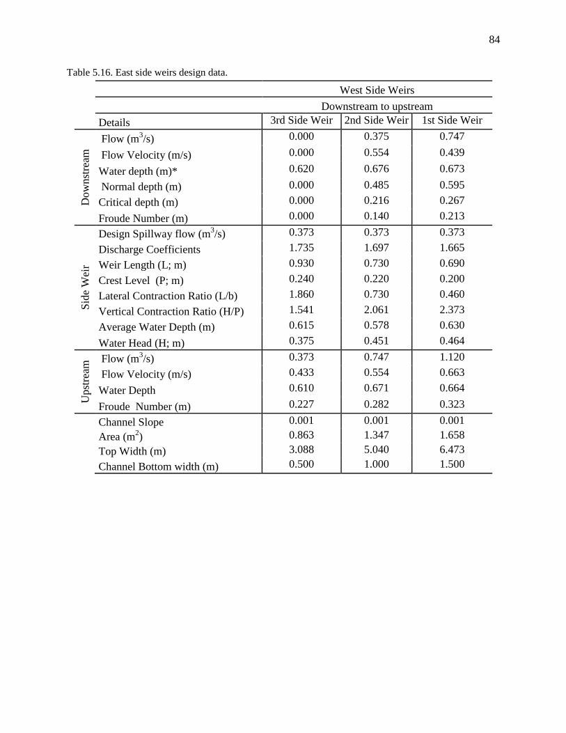
84
Table 5.16. East side weirs design data.
West Side Weirs
Downstream to upstream
Details 3rd Side Weir 2nd Side Weir 1st Side Weir
Dow
nst
ream
Flow (m3/s) 0.000 0.375 0.747
Flow Velocity (m/s) 0.000 0.554 0.439
Water depth (m)* 0.620 0.676 0.673
Normal depth (m) 0.000 0.485 0.595
Critical depth (m) 0.000 0.216 0.267
Froude Number (m) 0.000 0.140 0.213
Sid
e W
eir
Design Spillway flow (m3/s) 0.373 0.373 0.373
Discharge Coefficients 1.735 1.697 1.665
Weir Length (L; m) 0.930 0.730 0.690
Crest Level (P; m) 0.240 0.220 0.200
Lateral Contraction Ratio (L/b) 1.860 0.730 0.460
Vertical Contraction Ratio (H/P) 1.541 2.061 2.373
Average Water Depth (m) 0.615 0.578 0.630
Water Head (H; m) 0.375 0.451 0.464
Upst
ream
Flow (m3/s) 0.373 0.747 1.120
Flow Velocity (m/s) 0.433 0.554 0.663
Water Depth 0.610 0.671 0.664
Froude Number (m) 0.227 0.282 0.323
Channel Slope 0.001 0.001 0.001
Area (m
2) 0.863 1.347 1.658
Top Width (m) 3.088 5.040 6.473
Channel Bottom width (m) 0.500 1.000 1.500
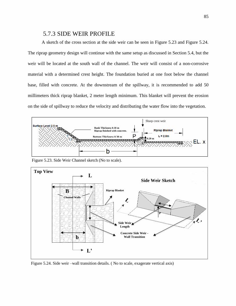
85
A sketch of the cross section at the side weir can be seen in Figure 5.23 and Figure 5.24.
The riprap geometry design will continue with the same setup as discussed in Section 5.4, but the
weir will be located at the south wall of the channel. The weir will consist of a non-corrosive
material with a determined crest height. The foundation buried at one foot below the channel
base, filled with concrete. At the downstream of the spillway, it is recommended to add 50
millimeters thick riprap blanket, 2 meter length minimum. This blanket will prevent the erosion
on the side of spillway to reduce the velocity and distributing the water flow into the vegetation.
5.7.3 SIDE WEIR PROFILE
Figure 5.23. Side Weir Channel sketch (No to scale).
Sharp crest weir
0.20 m Bottom Thickness 0.30 m
Bank Thickness 0.18 m
Riprap finished with concrete.
b
B
L’
L
Side Weir
Length
Top View
Concrete Side Weir -
Wall Transition
Side Weir Sketch
Riprap Blanket
Channel Walls
Figure 5.24. Side weir –wall transition details. ( No to scale, exagerate vertical axis)
P

86
It is important to identify and verify the shapes of the water surface before start modeling
any system. This water surface shapes will determine the relationship between the stage and the
discharge (Sturm, 2011). This shapes also, helps to determine if the water depth is decreasing
downstream. The tool that helps to determine water depth changes is the equation of gradually
varied flow (Chow, 1959, and Sturm, 2011):
5.39
where:
S0 = channel bottom slope,
Sf = energy slope or friction slope,
= ⁄ ,
Q = weir discharge,
= energy coefficient (assume 1),
qweir = discharge ratio per unit length ⁄ ,
g = acceleration of gravity,
A = area, and
F = Froude number (equation 5.23).
The importance to predict the water surface profile on the side weirs is that it helps to
determine the increase or decrease of water depth along the effective length of the weir. Figure
5.25 shows several types of water depth profiles and they will depend on the local depth (Y), the
normal depth (Yn) and the critical depth (Yc). Also the Froude number, the bottom slope and the
energy slope of the system have a big role to determine the type of profile required.
5.7.4 VERIFICATION OF WATER SURFACE PROFILE
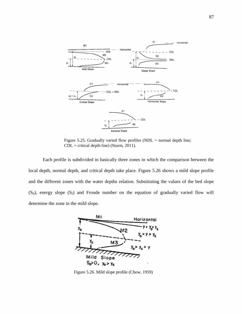
87
Figure 5.26. Mild slope profile (Chow, 1959)
Each profile is subdivided in basically three zones in which the comparison between the
local depth, normal depth, and critical depth take place. Figure 5.26 shows a mild slope profile
and the different zones with the water depths relation. Substituting the values of the bed slope
(S0), energy slope (Sf) and Froude number on the equation of gradually varied flow will
determine the zone in the mild slope.
Figure 5.25. Gradually varied flow profiles (NDL = normal depth line;
CDL = critical depth line) (Sturm, 2011).
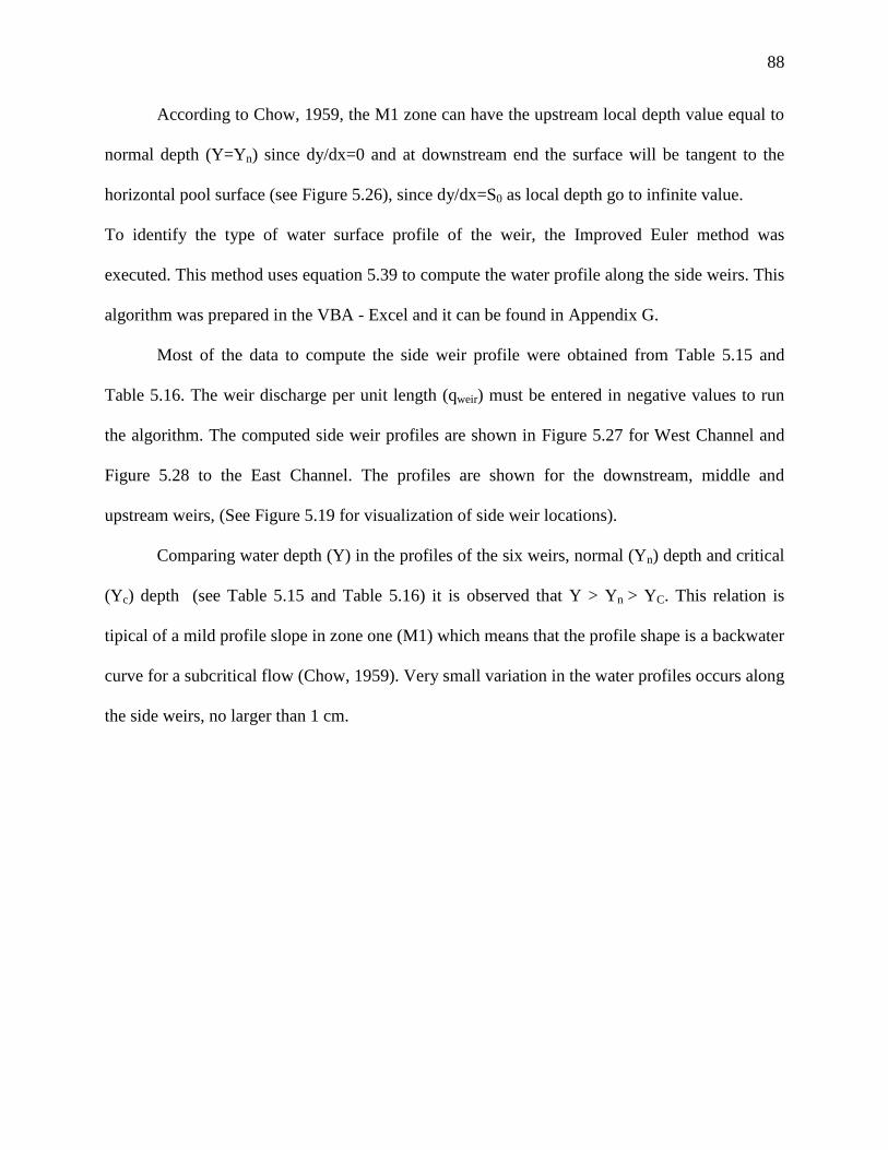
88
According to Chow, 1959, the M1 zone can have the upstream local depth value equal to
normal depth (Y=Yn) since dy/dx=0 and at downstream end the surface will be tangent to the
horizontal pool surface (see Figure 5.26), since dy/dx=S0 as local depth go to infinite value.
To identify the type of water surface profile of the weir, the Improved Euler method was
executed. This method uses equation 5.39 to compute the water profile along the side weirs. This
algorithm was prepared in the VBA - Excel and it can be found in Appendix G.
Most of the data to compute the side weir profile were obtained from Table 5.15 and
Table 5.16. The weir discharge per unit length (qweir) must be entered in negative values to run
the algorithm. The computed side weir profiles are shown in Figure 5.27 for West Channel and
Figure 5.28 to the East Channel. The profiles are shown for the downstream, middle and
upstream weirs, (See Figure 5.19 for visualization of side weir locations).
Comparing water depth (Y) in the profiles of the six weirs, normal (Yn) depth and critical
(Yc) depth (see Table 5.15 and Table 5.16) it is observed that Y > Yn > YC. This relation is
tipical of a mild profile slope in zone one (M1) which means that the profile shape is a backwater
curve for a subcritical flow (Chow, 1959). Very small variation in the water profiles occurs along
the side weirs, no larger than 1 cm.
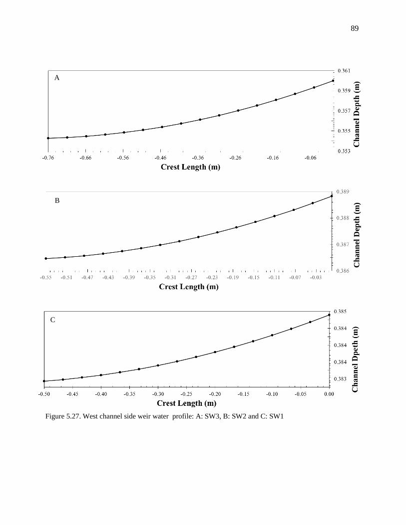
89
Figure 5.27. West channel side weir water profile: A: SW3, B: SW2 and C: SW1
A
B
C
Ch
an
nel
Dep
th (
m)
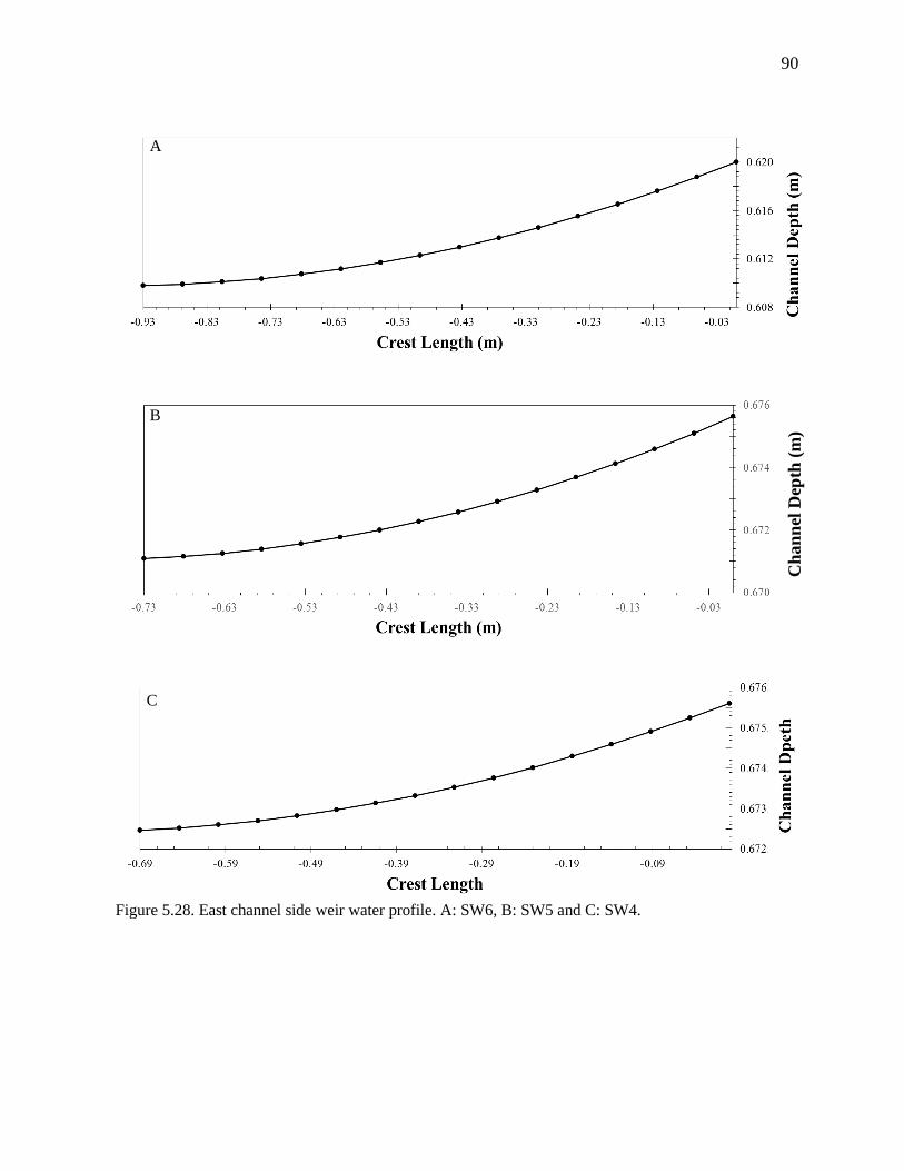
90
Figure 5.28. East channel side weir water profile. A: SW6, B: SW5 and C: SW4.
A
B
C
Ch
an
nel
Dep
th (
m)

91
Table 5.17 and Table 5.18, show the computed water depths at each of the sections along
the channel for the design flow without any freeboard overflow occur under design conditions. In
the West Channel, the maximum depth is 0.39 meters and the East Channel has a maximum
depth of 0.77 meters.
The designed channels have a recommended depth of 0.40 m and 0.80 m for channels
West and East, respectively. No provision for freeboard is given because there is no risk in case
of channel overflows. Both channel depths were chosen based on the maximum water depths
obtained in the computation. The channel is designed to distribute the flow through side weirs as
long as the discharge is less than the design value. The geometry design has to ensure that
flooding does not occur upstream, but flooding downstream into the AOI would be acceptable
for large events because that is the purpose of the design and operation of the channels. In the
discussion of the modeling of the channels, there will be a sensitivity analysis to see the flow
behavior caused by different events.
5.8 RECOMMENDED CHANNEL DIMENSIONS
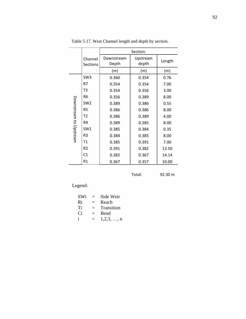
92
Section:
Channel Sections
Downstream Depth
Upstream depth
Length
(m) (m) (m)
Do
wn
stream to
Up
stream
SW3 0.360 0.354 0.76
R7 0.354 0.354 7.00
T3 0.354 0.356 3.00
R6 0.356 0.389 8.00
SW2 0.389 0.386 0.55
R5 0.386 0.386 8.00
T2 0.386 0.389 4.00
R4 0.389 0.385 8.00
SW1 0.385 0.384 0.35
R3 0.384 0.385 8.00
T1 0.385 0.391 7.00
R2 0.391 0.382 13.50
C1 0.382 0.367 14.14
R1 0.367 0.357 10.00
Total: 92.30 m
Table 5.17. West Channel length and depth by section.
Legend:
SWi = Side Weir
Ri = Reach
Ti = Transition
Ci = Bend
i = 1,2,3, …, n
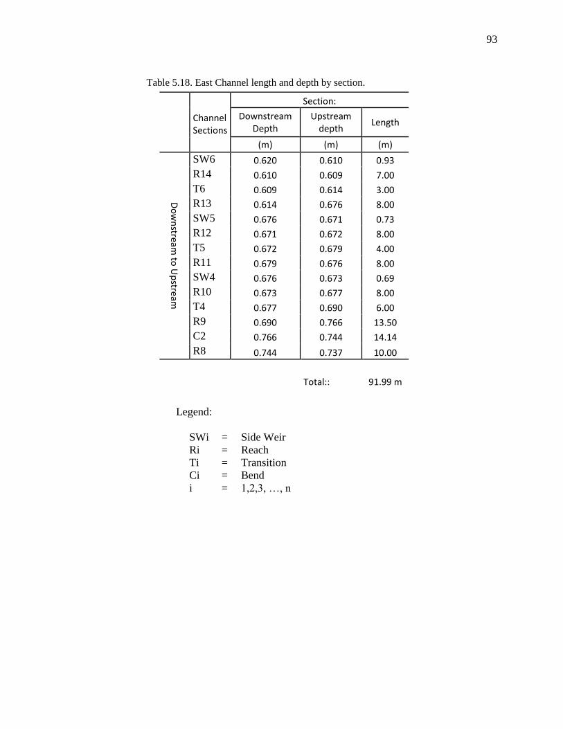
93
Section:
Channel Sections
Downstream Depth
Upstream depth
Length
(m) (m) (m)
Do
wn
stream to
Up
stream
SW6 0.620 0.610 0.93
R14 0.610 0.609 7.00
T6 0.609 0.614 3.00
R13 0.614 0.676 8.00
SW5 0.676 0.671 0.73
R12 0.671 0.672 8.00
T5 0.672 0.679 4.00
R11 0.679 0.676 8.00
SW4 0.676 0.673 0.69
R10 0.673 0.677 8.00
T4 0.677 0.690 6.00
R9 0.690 0.766 13.50
C2 0.766 0.744 14.14
R8 0.744 0.737 10.00
Total:: 91.99 m
Table 5.18. East Channel length and depth by section.
Legend:
SWi = Side Weir
Ri = Reach
Ti = Transition
Ci = Bend
i = 1,2,3, …, n
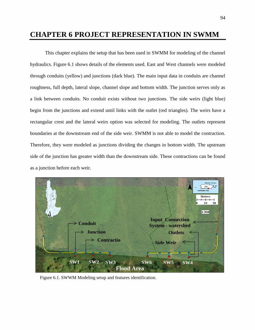
94
CHAPTER 6 PROJECT REPRESENTATION IN SWMM
This chapter explains the setup that has been used in SWMM for modeling of the channel
hydraulics. Figure 6.1 shows details of the elements used. East and West channels were modeled
through conduits (yellow) and junctions (dark blue). The main input data in conduits are channel
roughness, full depth, lateral slope, channel slope and bottom width. The junction serves only as
a link between conduits. No conduit exists without two junctions. The side weirs (light blue)
begin from the junctions and extend until links with the outlet (red triangles). The weirs have a
rectangular crest and the lateral weirs option was selected for modeling. The outlets represent
boundaries at the downstream end of the side weir. SWMM is not able to model the contraction.
Therefore, they were modeled as junctions dividing the changes in bottom width. The upstream
side of the junction has greater width than the downstream side. These contractions can be found
as a junction before each weir.
Conduit
Junction
ContractioSide Weir
Outlets
Input Connection
System - watershed
Flood Area
SW2 SW6 SW1 SW3
Figure 6.1. SWWM Modeling setup and features identification.
SW5 SW4
95
The Simulation Option window in SWMM allows the selection of the computation
method for infiltration and routing. Dynamic Wave flow routing was selected as routing method.
The SCS Curve Number Method was selected as the infiltration method. As previously mention,
the historical event of August 8, 2011 was used as design event. Additional details about the
subwatersheds areas, roughness values and other parameters can be found in previous sections.
The hydraulic model of SWMM will dictate the flow behavior in the design system for given
conditions. The objective of this design is to distribute evenly the spill flow through three side weirs.
This objective is applicable to the East and West Channels. Figure 6.2 and Figure 6.3 shows the
flow distribution for each weir for the design storm measured in August 22, 2011. Both channels
have a similar distribution pattern. When the rain intensity stays less than 10 mm/hr all weirs have
the same pattern of distribution. Approximately at 2:45 PM there was an increase the amount of rain.
The flow at that moment for the West channel was an average of 0.022 m3/s over each side weir.
Furthermore, the East Channel, for the same time period, has an average of 0.085 m3/s.
The maximum spill flow over the weirs occurs at 11:00 P.M. which produces output
discharges of 0.102, 0.099, and 1.29 m3/s (weirs spill flow upstream to downstream) in West Channel
weir. The East channel have similar spill flow pattern, the flows produced by the models are 0.328,
0.325, and 0.402 m3/s (weirs spill flow from upstream to downstream).
The spill flows values obtained in SWMM do no match with the design weir flows. The
design was computed using the energy equations, mass balance, and side weir equation along the
channel from downstream to upstream. The design spill flow for each side weirs were 0.117 for the
West Channel and 0.373 for the East Channel. These differences in values between modeling and
design values are associated to the computation equations used in each method. The modeling
6.1 MODELING DESIGN
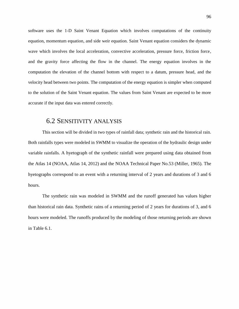
96
software uses the 1-D Saint Venant Equation which involves computations of the continuity
equation, momentum equation, and side weir equation. Saint Venant equation considers the dynamic
wave which involves the local acceleration, convective acceleration, pressure force, friction force,
and the gravity force affecting the flow in the channel. The energy equation involves in the
computation the elevation of the channel bottom with respect to a datum, pressure head, and the
velocity head between two points. The computation of the energy equation is simpler when computed
to the solution of the Saint Venant equation. The values from Saint Venant are expected to be more
accurate if the input data was entered correctly.
This section will be divided in two types of rainfall data; synthetic rain and the historical rain.
Both rainfalls types were modeled in SWMM to visualize the operation of the hydraulic design under
variable rainfalls. A hyetograph of the synthetic rainfall were prepared using data obtained from
the Atlas 14 (NOAA, Atlas 14, 2012) and the NOAA Technical Paper No.53 (Miller, 1965). The
hyetographs correspond to an event with a returning interval of 2 years and durations of 3 and 6
hours.
The synthetic rain was modeled in SWMM and the runoff generated has values higher
than historical rain data. Synthetic rains of a returning period of 2 years for durations of 3, and 6
hours were modeled. The runoffs produced by the modeling of those returning periods are shown
in Table 6.1.
6.2 SENSITIVITY ANALYSIS
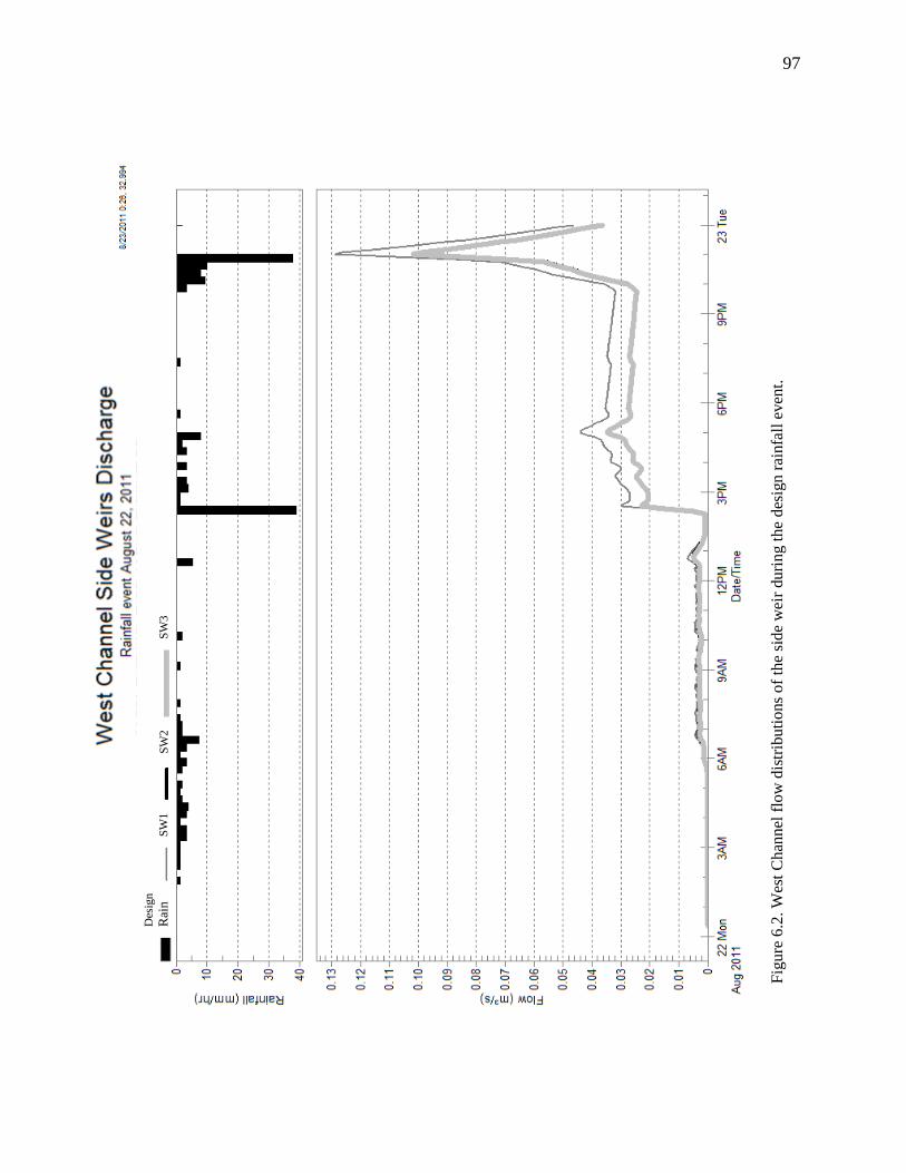
97
Fig
ure
6.2
. W
est
Ch
ann
el f
low
dis
trib
uti
ons
of
the
side
wei
r duri
ng t
he d
esig
n r
ainfa
ll e
ven
t.
Des
ign
Rai
n
SW
1
SW
2
SW
3
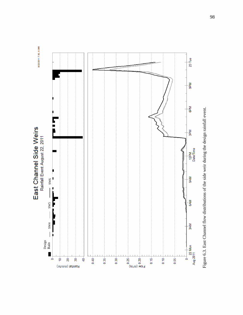
98
Fig
ure
6.3
. E
ast
Chan
nel
flo
w d
istr
ibu
tio
ns
of
the
sid
e w
eir
du
rin
g t
he
des
ign
rai
nfa
ll e
ven
t.
Des
ign
Rai
n
SW
4
SW
5
SW
6
99
Figure 6.4. Channel profile of the maximum water depth during August 22, 2011 rainfall event. A) West
Channel profile. B) East Channel Profile.
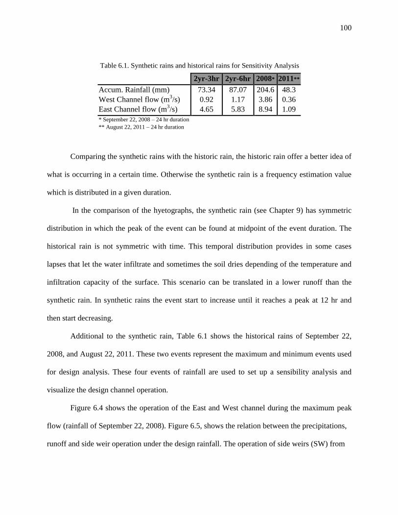
100
2yr-3hr 2yr-6hr 2008* 2011**
Accum. Rainfall (mm) 73.34 87.07 204.6 48.3
West Channel flow (m3/s) 0.92 1.17 3.86 0.36
East Channel flow (m3/s) 4.65 5.83 8.94 1.09
* September 22, 2008 – 24 hr duration
** August 22, 2011 – 24 hr duration
Comparing the synthetic rains with the historic rain, the historic rain offer a better idea of
what is occurring in a certain time. Otherwise the synthetic rain is a frequency estimation value
which is distributed in a given duration.
In the comparison of the hyetographs, the synthetic rain (see Chapter 9) has symmetric
distribution in which the peak of the event can be found at midpoint of the event duration. The
historical rain is not symmetric with time. This temporal distribution provides in some cases
lapses that let the water infiltrate and sometimes the soil dries depending of the temperature and
infiltration capacity of the surface. This scenario can be translated in a lower runoff than the
synthetic rain. In synthetic rains the event start to increase until it reaches a peak at 12 hr and
then start decreasing.
Additional to the synthetic rain, Table 6.1 shows the historical rains of September 22,
2008, and August 22, 2011. These two events represent the maximum and minimum events used
for design analysis. These four events of rainfall are used to set up a sensibility analysis and
visualize the design channel operation.
Figure 6.4 shows the operation of the East and West channel during the maximum peak
flow (rainfall of September 22, 2008). Figure 6.5, shows the relation between the precipitations,
runoff and side weir operation under the design rainfall. The operation of side weirs (SW) from
Table 6.1. Synthetic rains and historical rains for Sensitivity Analysis

101
this profile event are shown in Figure 6.5.C and Figure 6.5.D. The general information of the
side weirs can be found in Section 5.7. The design was done considering the rainfall which
creates the maximum runoff that could be captured by the channels without overflowing. There
is no risk of human hazard on the area and also this AOI belongs to the one of driest zones of
Puerto Rico. The design must divert the water and distribute the flow as uniform over the area as
possible, in order to be flooding the area. For larger rainfall events, the channel overflows
producing an increase in water level, velocity and shear stresses in the channels walls and bed.
According to computations, the shear forces produced by the design flow are five to six times
smaller than those that the channel can resists. Therefore, the design is capable to resist overflow.
The Figure 6.5.B shows the comparison between the runoff and the design flow for both
channels. This runoff conditions belongs to the rainfall of August of 2011. The design flows
chosen for this project are the peak runoff caused by this event.
Figure 6.6 is an example of the full water depth in the channels during the peak rainfall
event (September 22, 2008). These profiles show that no overflow occurs along the channel
during this event. Furthermore it is possible that upstream of the channel can be affected by the
runoff accumulation. The Figure 6.7.B shows runoff exceeding the design capacity, producing
flooding conditions until the amount of water decreases. The weirs will be overflowing until the
runoff reaches the design flow capacity. The modeling of this event was extended during the 5
days to show the channel operation during surcharge conditions.
The Figure 6.7.C and Figure 6.7.D shows the operation of the side weirs during
overflowing. The spill flow pattern will continue at the maximum level until the channel flow
decreases to the normal design flow. The figures show the increases of spill flow until they reach
a maximum point and then the flow decreases reaching the design flow.
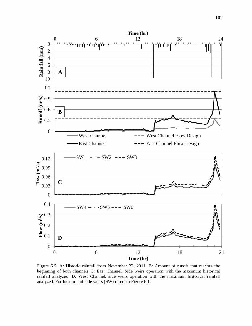
102
Figure 6.5. A: Historic rainfall from November 22, 2011. B: Amount of runoff that reaches the
beginning of both channels C: East Channel. Side weirs operation with the maximum historical
rainfall analyzed. D: West Channel. side weirs operation with the maximum historical rainfall
analyzed. For localtion of side weirs (SW) refers to Figure 6.1.
0
2
4
6
8
10
0 6 12 18 24R
ain
fall
(m
m)
Time (hr)
0
0.3
0.6
0.9
1.2
Ru
noff
(m
3/s
)
West Channel West Channel Flow Design
East Channel East Channel Flow Design
0
0.03
0.06
0.09
0.12
Flo
w (
m3/s
)
SW1 SW2 SW3
0
0.1
0.2
0.3
0.4
0 6 12 18 24
Flo
w (
m3/s
)
Time (hr)
SW4 SW5 SW6
C
A
D
B
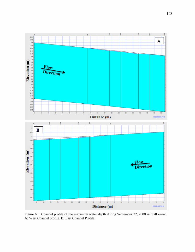
103
A
Figure 6.6. Channel profile of the maximum water depth during September 22, 2008 rainfall event.
A) West Channel profile. B) East Channel Profile.
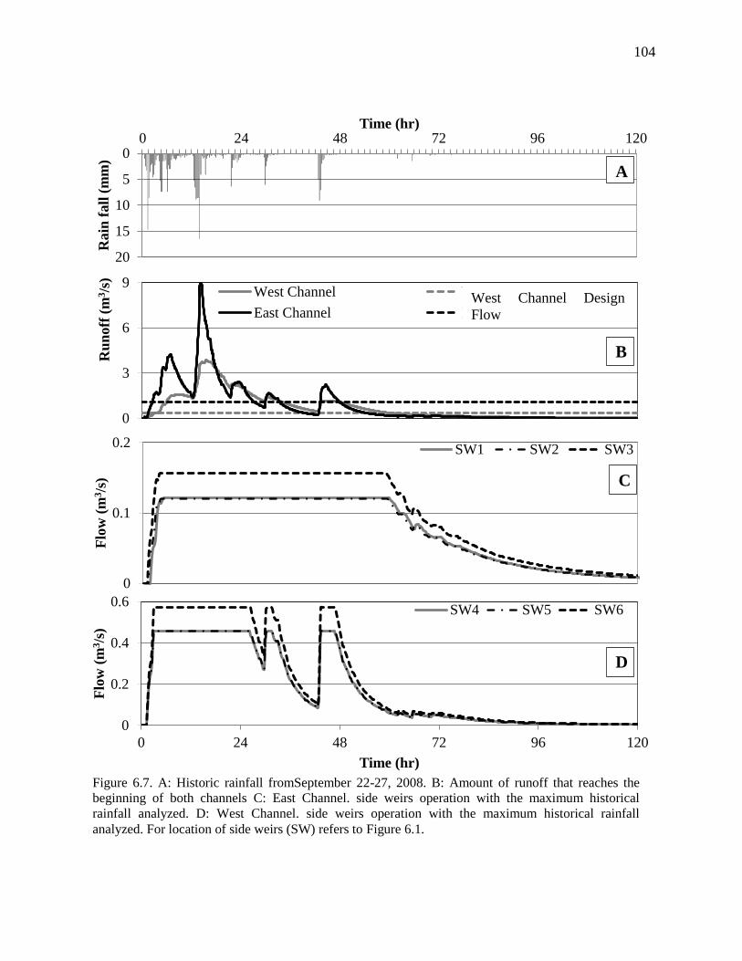
104
0
5
10
15
20
0 24 48 72 96 120
Rain
fall
(m
m)
Time (hr)
0
0.2
0.4
0.6
0 24 48 72 96 120
Flo
w (
m3/s
)
Time (hr)
SW4 SW5 SW6
0
0.1
0.2
Flo
w (
m3/s
)
SW1 SW2 SW3
C
A
D
Figure 6.7. A: Historic rainfall fromSeptember 22-27, 2008. B: Amount of runoff that reaches the
beginning of both channels C: East Channel. side weirs operation with the maximum historical
rainfall analyzed. D: West Channel. side weirs operation with the maximum historical rainfall
analyzed. For location of side weirs (SW) refers to Figure 6.1.
0
3
6
9
Ru
noff
(m
3/s
)
West Channel West Channel Flow Design
East Channel East Channel Flow Design
B
West Channel Design
Flow
West Channel Design
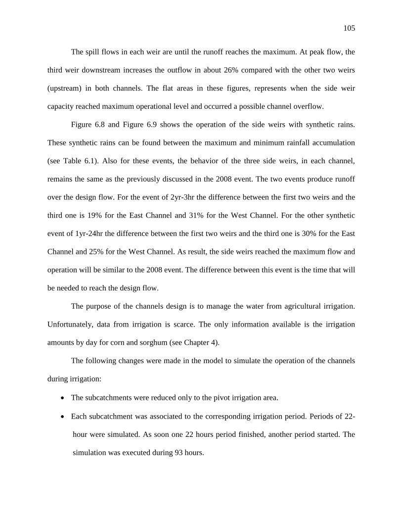
105
The spill flows in each weir are until the runoff reaches the maximum. At peak flow, the
third weir downstream increases the outflow in about 26% compared with the other two weirs
(upstream) in both channels. The flat areas in these figures, represents when the side weir
capacity reached maximum operational level and occurred a possible channel overflow.
Figure 6.8 and Figure 6.9 shows the operation of the side weirs with synthetic rains.
These synthetic rains can be found between the maximum and minimum rainfall accumulation
(see Table 6.1). Also for these events, the behavior of the three side weirs, in each channel,
remains the same as the previously discussed in the 2008 event. The two events produce runoff
over the design flow. For the event of 2yr-3hr the difference between the first two weirs and the
third one is 19% for the East Channel and 31% for the West Channel. For the other synthetic
event of 1yr-24hr the difference between the first two weirs and the third one is 30% for the East
Channel and 25% for the West Channel. As result, the side weirs reached the maximum flow and
operation will be similar to the 2008 event. The difference between this event is the time that will
be needed to reach the design flow.
The purpose of the channels design is to manage the water from agricultural irrigation.
Unfortunately, data from irrigation is scarce. The only information available is the irrigation
amounts by day for corn and sorghum (see Chapter 4).
The following changes were made in the model to simulate the operation of the channels
during irrigation:
The subcatchments were reduced only to the pivot irrigation area.
Each subcatchment was associated to the corresponding irrigation period. Periods of 22-
hour were simulated. As soon one 22 hours period finished, another period started. The
simulation was executed during 93 hours.

106
The daily irrigation volume was divided into 22 hours/day.
The irrigation process consist in apply the irrigation in one quarter of the crop circle at a
time.
Irrigation intensity was 0.703 mm/hr (NRCS, 2009).
Curve numbers and Manning roughness, were transferred from the original
subcatchment.
Figure 6.10.A shows the modeling results of the runoff produced by the irrigation which
reaches each channel. The maximum runoff produced by the irrigation was around 0.009 m3/s,
which is below the design condition for both channels. As a consequence, the spill flow profiles
of the weirs have the same pattern as the runoff (see Figure 6.10.B and Figure 6.10.C).
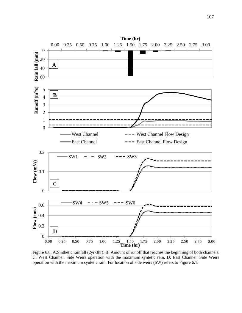
107
Figure 6.8. A:Sinthetic rainfall (2yr-3hr). B: Amount of runoff that reaches the beginning of both channels.
C: West Channel. Side Weirs operation with the maximum syntetic rain. D: East Channel. Side Weirs
operation with the maximum syntetic rain. For location of side weirs (SW) refers to Figure 6.1.
0
1
2
3
4
5
Ru
no
ff (
m3/s
)
West Channel West Channel Flow Design
East Channel East Channel Flow Design
0
0.1
0.2
Flo
w (
m3/s
)
SW1 Series2 SW3SW2
0
0.2
0.4
0.6
0.00 0.25 0.50 0.75 1.00 1.25 1.50 1.75 2.00 2.25 2.50 2.75 3.00
Flo
w (
cms)
Time (hr)
SW4 SW5 SW6
0
20
40
60
0.00 0.25 0.50 0.75 1.00 1.25 1.50 1.75 2.00 2.25 2.50 2.75 3.00
Rain
fall
(m
m)
Time (hr)
A
B
C
D
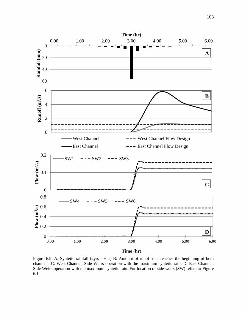
108
Figure 6.9. A: Syntetic rainfall (2yrs – 6hr) B: Amount of runoff that reaches the beginning of both
channels. C: West Channel. Side Weirs operation with the maximum syntetic rain. D: East Channel.
Side Weirs operation with the maximum syntetic rain. For location of side weirs (SW) refers to Figure
6.1.
0
2
4
6
Ru
noff
(m
3/s
)
West Channel West Channel Flow Design
East Channel East Channel Flow Design
0
20
40
60
0.00 1.00 2.00 3.00 4.00 5.00 6.00R
ain
fall
(m
m)
Time (hr)
0
0.1
0.2
Flo
w (
m3/s
)
SW1 SW2 SW3
0
0.2
0.4
0.6
0.8
0.00 1.00 2.00 3.00 4.00 5.00 6.00
Flo
w (
m3/s
)
SW4 SW5 SW6
C
D
B
A
Time (hr)
109
0
0.001
0.002
0.003
0.004
Flo
w (
m3/s
)
SW1 SW2 SW3
Figure 6.10. A: Amount of runoff that reaches the beginning of both channels (sorghum irrigation data) B:
East Channel. Side Weirs operation during irrigation process. C: East Channel. Side Weirs operation during
irrigation process. For location of side weirs (SW) refers to Figure 6.1.
A
B
C
0
0.001
0.002
0.003
0.004
0.00 48.00 96.00 144.00 192.00 240.00
Flo
w (
m3/s
)
Time (hr)
SW4 SW5 SW6
0
0.002
0.004
0.006
0.008
0.01
Ru
no
ff (
m3/s
)
West Channel East Channel
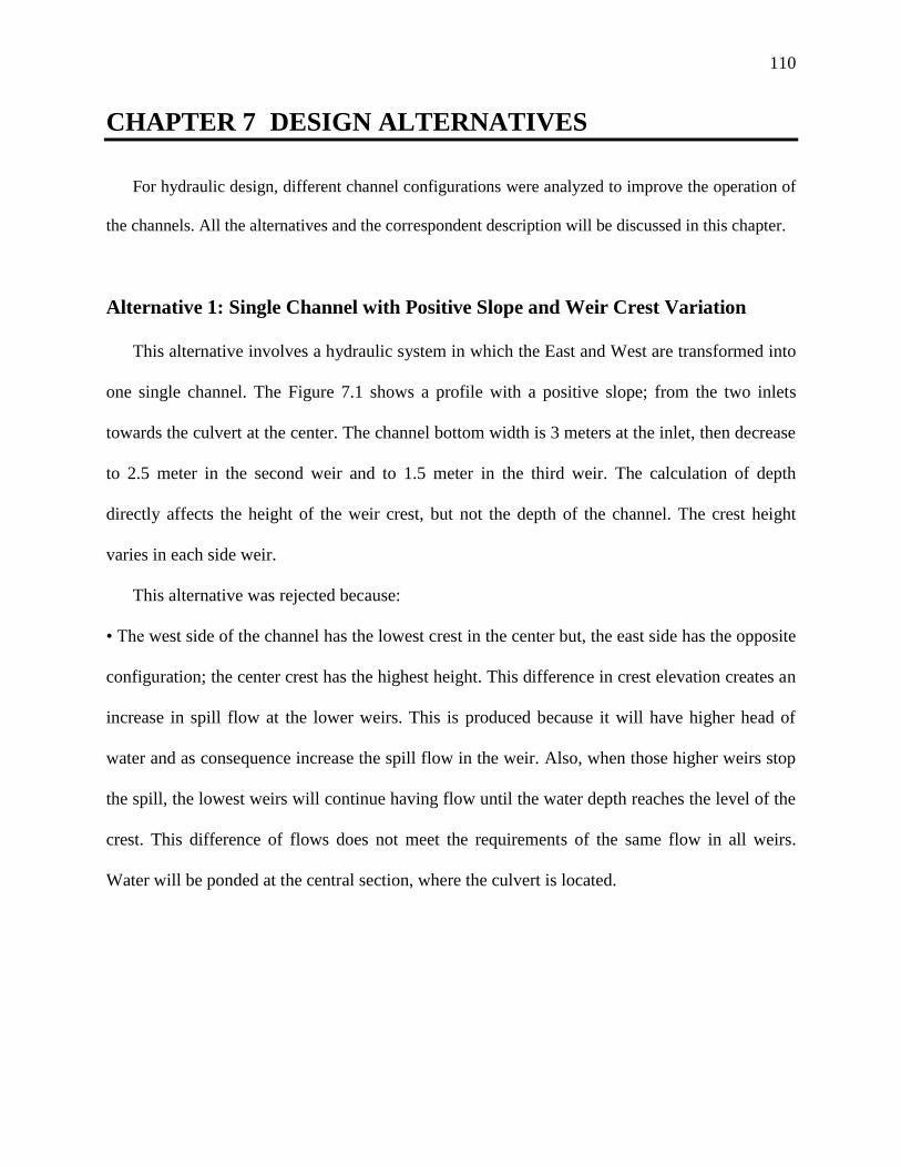
110
CHAPTER 7 DESIGN ALTERNATIVES
For hydraulic design, different channel configurations were analyzed to improve the operation of
the channels. All the alternatives and the correspondent description will be discussed in this chapter.
Alternative 1: Single Channel with Positive Slope and Weir Crest Variation
This alternative involves a hydraulic system in which the East and West are transformed into
one single channel. The Figure 7.1 shows a profile with a positive slope; from the two inlets
towards the culvert at the center. The channel bottom width is 3 meters at the inlet, then decrease
to 2.5 meter in the second weir and to 1.5 meter in the third weir. The calculation of depth
directly affects the height of the weir crest, but not the depth of the channel. The crest height
varies in each side weir.
This alternative was rejected because:
• The west side of the channel has the lowest crest in the center but, the east side has the opposite
configuration; the center crest has the highest height. This difference in crest elevation creates an
increase in spill flow at the lower weirs. This is produced because it will have higher head of
water and as consequence increase the spill flow in the weir. Also, when those higher weirs stop
the spill, the lowest weirs will continue having flow until the water depth reaches the level of the
crest. This difference of flows does not meet the requirements of the same flow in all weirs.
Water will be ponded at the central section, where the culvert is located.
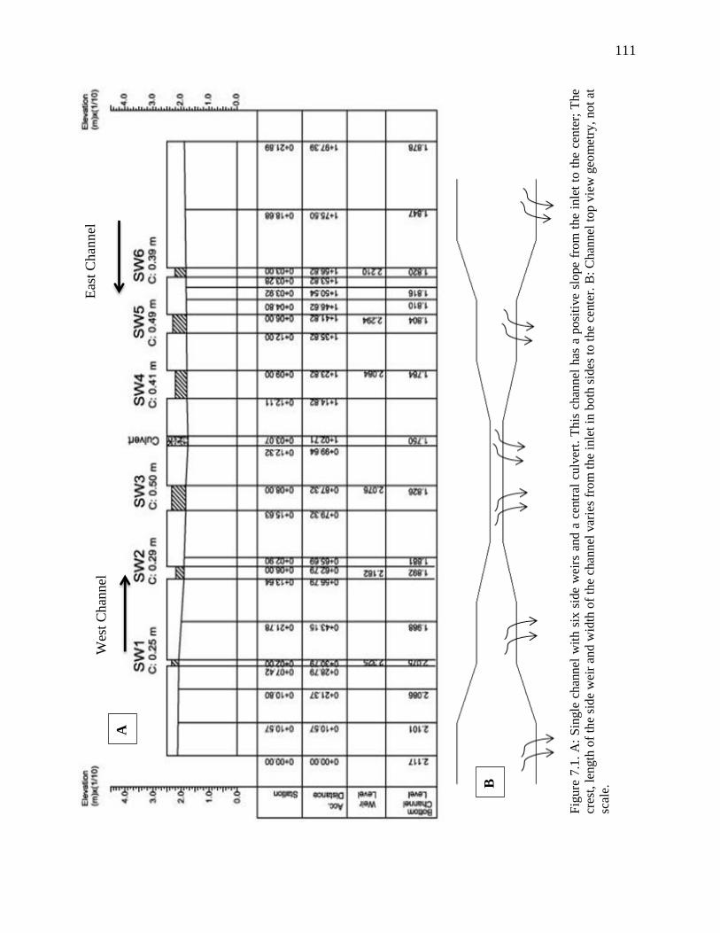
111
Fig
ure
7.1
. A
: S
ingle
ch
ann
el w
ith s
ix s
ide
wei
rs a
nd a
cen
tral
culv
ert.
This
chan
nel
has
a p
osi
tive
slo
pe
fro
m t
he
inle
t to
th
e ce
nte
r; T
he
cres
t, l
ength
of
the
sid
e w
eir
and
wid
th o
f th
e ch
annel
var
ies
from
the
inle
t in
both
sid
es t
o t
he
cente
r. B
: C
han
nel
to
p v
iew
geo
met
ry,
no
t at
scal
e.
Eas
t C
han
nel
W
est
Chan
nel
A
B
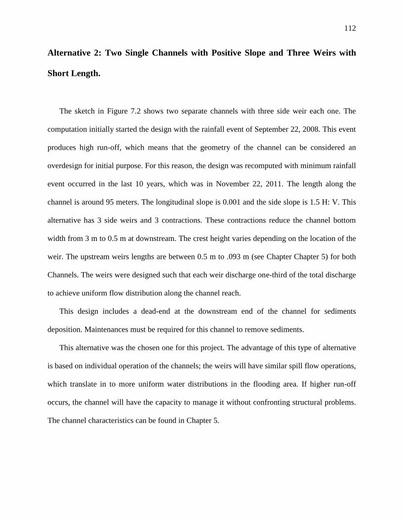
112
Alternative 2: Two Single Channels with Positive Slope and Three Weirs with
Short Length.
The sketch in Figure 7.2 shows two separate channels with three side weir each one. The
computation initially started the design with the rainfall event of September 22, 2008. This event
produces high run-off, which means that the geometry of the channel can be considered an
overdesign for initial purpose. For this reason, the design was recomputed with minimum rainfall
event occurred in the last 10 years, which was in November 22, 2011. The length along the
channel is around 95 meters. The longitudinal slope is 0.001 and the side slope is 1.5 H: V. This
alternative has 3 side weirs and 3 contractions. These contractions reduce the channel bottom
width from 3 m to 0.5 m at downstream. The crest height varies depending on the location of the
weir. The upstream weirs lengths are between 0.5 m to .093 m (see Chapter Chapter 5) for both
Channels. The weirs were designed such that each weir discharge one-third of the total discharge
to achieve uniform flow distribution along the channel reach.
This design includes a dead-end at the downstream end of the channel for sediments
deposition. Maintenances must be required for this channel to remove sediments.
This alternative was the chosen one for this project. The advantage of this type of alternative
is based on individual operation of the channels; the weirs will have similar spill flow operations,
which translate in to more uniform water distributions in the flooding area. If higher run-off
occurs, the channel will have the capacity to manage it without confronting structural problems.
The channel characteristics can be found in Chapter 5.
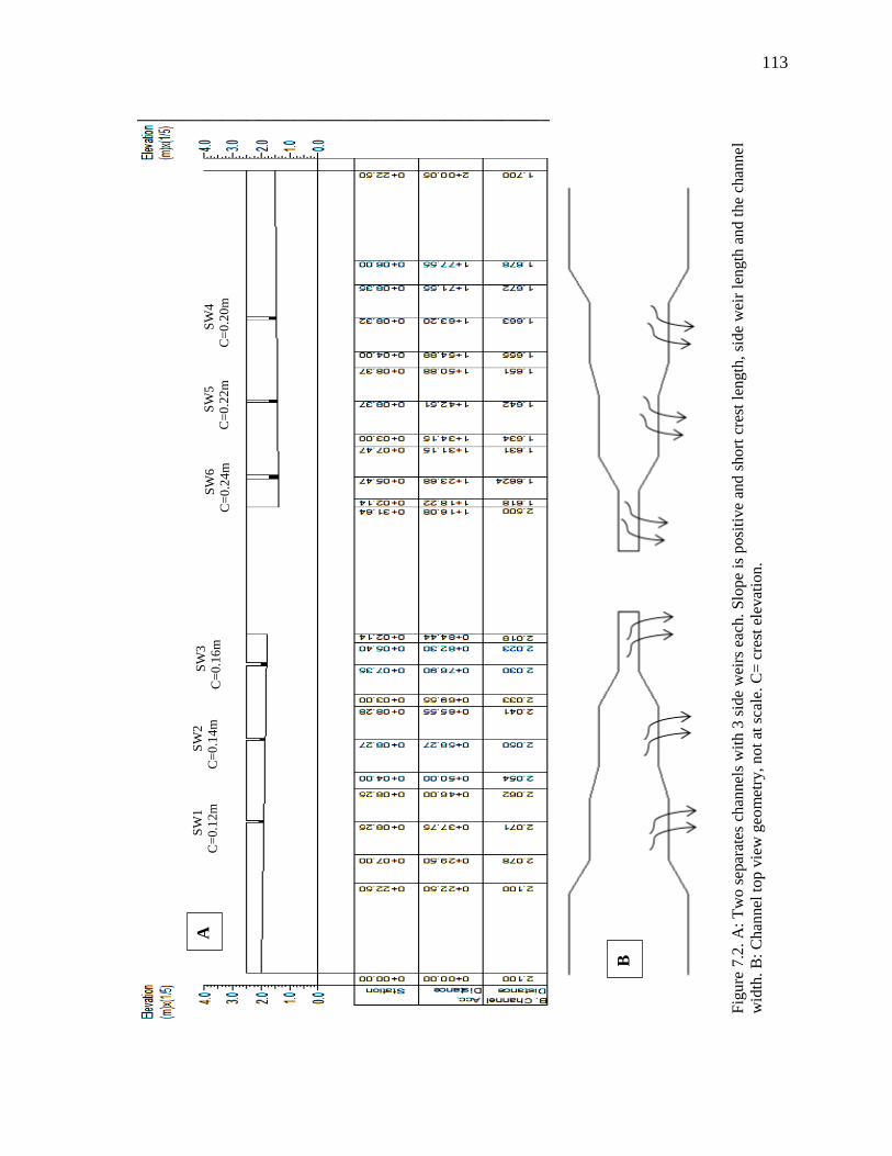
113
Fig
ure
7.2
. A
: T
wo s
epar
ates
ch
annel
s w
ith 3
sid
e w
eirs
eac
h.
Slo
pe
is p
osi
tive
and s
hort
cre
st l
ength
, si
de
wei
r le
ngth
an
d t
he
chan
nel
wid
th.
B:
Ch
annel
to
p v
iew
geo
met
ry,
not
at s
cale
. C
= c
rest
ele
vat
ion.
SW
1
C=
0.1
2m
SW
2
C=
0.1
4m
S
W3
C=
0.1
6m
S
W4
C=
0.2
0m
SW
5
C=
0.2
2m
S
W6
C=
0.2
4m
A
B

114
CHAPTER 8 ANALYSIS AND DISCUSION
Historically, the north area of the Jobos Reserve has been very active as far as agriculture
is concerned. An irrigation pivot system was installed in the area in 1994. The irrigation system
increased the amount of runoff flows carrying fertilizers and other chemical compounds used for
agriculture, that impacted protected areas. The mangrove area has decreased during the last
decade. Hurricane George in 1998 significantly affected the area and caused great damage to the
mangrove. The mangrove recovery has not been successful since those events.
Jobos Reserve, specifically the north of Mar Negro, has a geology where the main
component is alluvium material. The climatic condition of the area is quite wet during the rainy
season, from September to October and the driest month in January.
The hydrological analysis began with the delineation of basins and sub-basins in ArcGIS,
using a USGS topographic map, aerial photography (USACE) and field work. The roughness
coefficients for overland flow were obtained from the SCS website by entering the watershed as
the area of interest. Other variables determined for overland flow computation were the
precipitation for design and the abstractions:
The abstraction method evaluated was the Curve Number method (CN). This method was
used to estimate the infiltration from the runoff. The CN values were obtained using high
resolution aerial photos, field work and a GIS shapefile of Puerto Rico CN prepared by
the SCS.
The maximum precipitation accumulation during a 24 hr period of historic data was
produced in September 22, 2008, which was 204.6 mm. The lowest precipitation in the
10 years analyzed occurred in November 22, 2011 which was 48.7 mm. From the
analysis of the current study, the rainfall of 2008 and 2011 produced a total runoff of
115
12.58 m3/s and 1.35 m
3/s, respectively. The 2008 peak runoff produced a 3.86 m
3/s
reaching the West Channel and 8.94 m3/s reaching the East Channel. The 2011 peak
runoff can be divided in 0.36 m3/s reaching the West Channel and 1.09 m
3/s for the East
Channel inlet.
The rainfall of 2008 and 2011 were equivalent to a frequency event of 10 yr. and
1 yr, respectively. The synthetic event of 1 yr – 24 hr. (see Appendix H) was modeled
and compared with the 2011 historical rainfall. This synthetic rain produces a total runoff
of 1.73 m3/s which is distributed by the model in 0.75 m
3/s for West Channel and 0.98
m3/s for East Channel. The distribution of the synthetic rainfall have a notably effect on
the amount of runoff reaching both channel. This synthetic rain doubles the historic
rainfall runoff for both West and East Channel.
The 2011 event was chosen as design rain. This project does not represent any
risk for human beings and the design is for agricultural irrigations runoff management,
which are lower than this event. Irrigation discharge data available is scarce.
The only irrigation data that was obtained was for sorghum and corn. The sorghum
irrigation was modeled in this project to have a general idea of the operation of the
channels under this condition. The pivot circle was divided into 4 areas, of the same size.
According PRLA, the farmers irrigate a quarter of a circle at a time, for 22 hours per day
and at a rate of 0.703 mm/h.
Flow routing is a computational procedure used to predict the changes in magnitude,
speed and shape of a flood wave as a function of time at various points along river
channel (Maidment, 1992). Three options of routing methods, steady flow, kinematic
116
wave, and dynamic wave were introduced on Chapter 4. The method of dynamic wave
was chosen due to hydraulics considerations that will be discussed later on this chapter.
The hydraulic analysis started with the channel design modeled in SWMM:
A topographic survey of the study area for existing conditions was performed.
Currently, two trapezoidal channels (at the east and west of the AOI) are operating as
runoff collectors and discharging directly to the mangrove area in Jobos bay. The
West Channel has a depth of around 0.4 m at the outlet and it increases moving
upstream. The East Channel has a depth of 0.8 m and follows the same upstream
condition of the West Channel. Both channels have the maximum depth at the
boundary of the irrigation pivot circle. This location is the point in which the channels
start decreasing in depth upstream until they reach the beginning of the channels.
The new design involves two separate channels with 90 degrees bend toward the
center of the AOI. These channels will have a bottom width of 3 meters as the current
channels and they decrease until 0.5 meters at the end of the channel downstream.
Each channel distributes the runoff evenly as possible through 3 side weirs. The
channel depth is 0.40 m for West Channel and 0.75 m for the East Channel. The side
slope is 1.5 and longitudinal slope is 0.001 for both channels.
The channel lining analysis started with a comparison of different types of lining as
earth, cemented, riprap, and grouted riprap linings. The best lining was the riprap,
grouted riprap, and reinforced concrete. The reinforce concrete was rejected due the
high cost, Section 9.3 presents the cost estimates showing that the cost of concrete is
around six times the cost of grouted riprap. The riprap was grouted to eliminate the
possibility that an increase of flow can move the layer of rocks and decrease the
117
operational efficiency of the channel. Also, in riprap without grout the vegetation can
grow between rocks decreasing the flow velocities and increasing the maintenance
cost. The grouted riprap is low cost, the grouted layer provides rock stability and
decrease the cost of maintenance.
The lining design was prepared for a riprap size of 90 mm. This size of riprap can
produce a roughness of 0.032 but, the grout cement will increase approximately 13%
the roughness of the design liner. Other important criterion of design is the shear
stress in the channel's wall and bed. The critical shear stress, allowable for the
channel bed and walls, are 56.55 MPa and 31.36 MPa, respectively. The maximum
shear stress of the West Channel bed and wall exerted by the water flow are 3.38 MPa
and 2.70 MPa, respectively. The water flow in the East Channel bottom bed and side
wall produced a 5.63 MPa and 4.50 MPa, respectively. The channel liner will support
approximately 6% of critical shear stress in the bottom bed and 18% in the side wall.
In the channels bends design two main factors were considered: 1) the maximum
shear stress produced by the water flow shall not exceed the critical shear stress
allowable by the channel liner; and 2) the super elevation to prevent the overflow of
the channel due to the increase in water depth in bends. The maximum shear stress
produced in walls and bed by the water flow in the bend is 5.02 MPa (9%) and 6.28
MPa (20%), respectively. This maximum shear stress is low compared with the
critical shear stress allowable for the riprap design. The super elevation obtained from
the design is 0.05 m for the West Channel and 0.10 m for the East Channel.
The channels bottom width begins 3 meters upstream and reduces to 0.5 meters
downstream. These reductions occur by three inlet transitions in strategic locations.
118
The transition used was the straight line as recommended by FHWA (2012). All
transitions have a flare angle less than 12.5 degrees to keep subcritical flow along the
transition. Each transition is located before the weirs. The inlet transitions reduce the
width of the channel downstream, increasing the flow velocity and decreasing the
water depth.
The hydraulic design computations used three different equations; mass balance
equation, energy equation, and side weir equation. The selection of the weir equation
for design purposes required the discharge coefficient for a side weir condition. The
most important variables for the discharge coefficient computation are the crest
height and the water head. All discharge coefficient equations include these two
variables accompanied with other constants which depend on the experimental
conditions from which the equation was derived. For Froude numbers less than one
the side weir provides the most reliable operation. If the Froude number is higher than
one, there is a chance that a hydraulic jump occurs in the weir, decreasing the velocity
of the flow and causing a decrease in the operational efficiency. The discharge
coefficient proposed by Subramayan, K. and Awasthy, S. C. (Emiroglu, et. al, 2011)
was selected based on Chow, (1959), and French, (1987) recommendations. Also this
equation produces the higher discharge coefficient and similar values for the three
side weirs. The side weir equation requires similar discharge coefficient to adjust the
condition of length and crest height, in order of obtain similar spill flow in each one.
The water profile of the side weirs was computed using the Euler improves method
for side weirs (see Appendix G). This method use the equation of gradually varied
flow modified for weirs to estimate the water profile. The best side weir operation
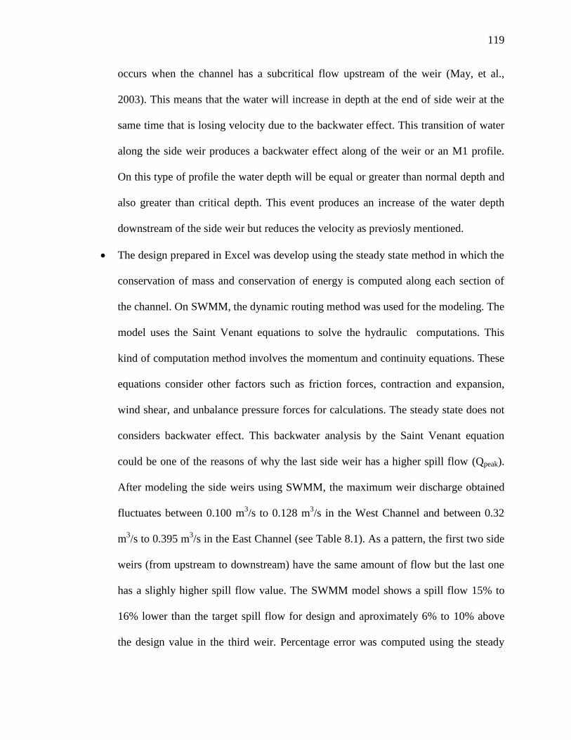
119
occurs when the channel has a subcritical flow upstream of the weir (May, et al.,
2003). This means that the water will increase in depth at the end of side weir at the
same time that is losing velocity due to the backwater effect. This transition of water
along the side weir produces a backwater effect along of the weir or an M1 profile.
On this type of profile the water depth will be equal or greater than normal depth and
also greater than critical depth. This event produces an increase of the water depth
downstream of the side weir but reduces the velocity as previosly mentioned.
The design prepared in Excel was develop using the steady state method in which the
conservation of mass and conservation of energy is computed along each section of
the channel. On SWMM, the dynamic routing method was used for the modeling. The
model uses the Saint Venant equations to solve the hydraulic computations. This
kind of computation method involves the momentum and continuity equations. These
equations consider other factors such as friction forces, contraction and expansion,
wind shear, and unbalance pressure forces for calculations. The steady state does not
considers backwater effect. This backwater analysis by the Saint Venant equation
could be one of the reasons of why the last side weir has a higher spill flow (Qpeak).
After modeling the side weirs using SWMM, the maximum weir discharge obtained
fluctuates between 0.100 m3/s to 0.128 m
3/s in the West Channel and between 0.32
m3/s to 0.395 m
3/s in the East Channel (see Table 8.1). As a pattern, the first two side
weirs (from upstream to downstream) have the same amount of flow but the last one
has a slighly higher spill flow value. The SWMM model shows a spill flow 15% to
16% lower than the target spill flow for design and aproximately 6% to 10% above
the design value in the third weir. Percentage error was computed using the steady
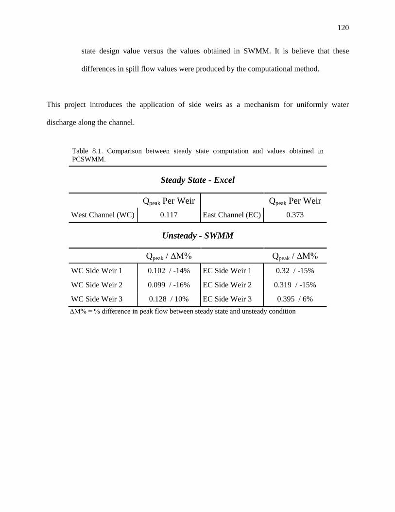
120
state design value versus the values obtained in SWMM. It is believe that these
differences in spill flow values were produced by the computational method.
This project introduces the application of side weirs as a mechanism for uniformly water
discharge along the channel.
Steady State - Excel
Qpeak Per Weir
Qpeak Per Weir
West Channel (WC) 0.117 East Channel (EC) 0.373
Unsteady - SWMM
Qpeak / ∆M%
Qpeak / ∆M%
WC Side Weir 1 0.102 / -14% EC Side Weir 1 0.32 / -15%
WC Side Weir 2 0.099 / -16% EC Side Weir 2 0.319 / -15%
WC Side Weir 3 0.128 / 10% EC Side Weir 3 0.395 / 6%
∆M% = % difference in peak flow between steady state and unsteady condition
Table 8.1. Comparison between steady state computation and values obtained in
PCSWMM.

121
CHAPTER 9 DESIGN RECOMENDATIONS
This Chapter includes all the additional recommendations that can be applied to the design of
the channel. Here are included the cross sections profiles with existent geometry, cut and fill
profiles and a conceptual cost estimate for design.
The area of interest (AOI) in Jobos has five north-south trails and other three west-east trails.
Two of the north-south trails, contains a battery of five piezometers each trail; the location of
these piezometers are shown as red dots in Figure 9.1. Taking advantage of these trails, the cross
sections were delineating at the middle trail (C-C’), west trail (A-A’) and east trails E-E’. The
cross sections B-B` and C-C’ are placed following the line of piezometers as shown in Figure
9.1. These cross sections delineate the current conditions of the AOI as maximum elevation,
minimum elevations and slope. At north, the line I-I’ is a representation of the profile in which
the channel location is proposed. The north boundary of the AOI has a maximum elevation of
approximately 2.5 meter above mean sea level (a.m.s.l.) and a minimum elevation of about 0.6
meters a.m.s.l. at the south end; with a slope around 0.8%.
The current topography of the area is represented in the cross sections shown from Figure 9.2
to Figure 9.7. The locations of these cross sections in the AOI are shown in Figure 9.1
9.1 LAND SURVEY
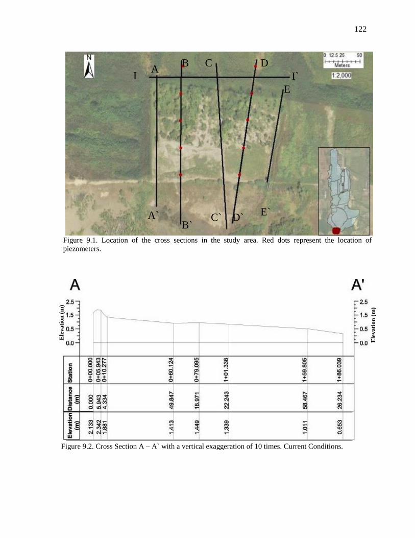
122
A` B`
C` D` E`
E
D C B A
Figure 9.1. Location of the cross sections in the study area. Red dots represent the location of
piezometers.
I I`
Figure 9.2. Cross Section A – A` with a vertical exaggeration of 10 times. Current Conditions.
Ele
vati
on
(m
)
Ele
vati
on
(m
)
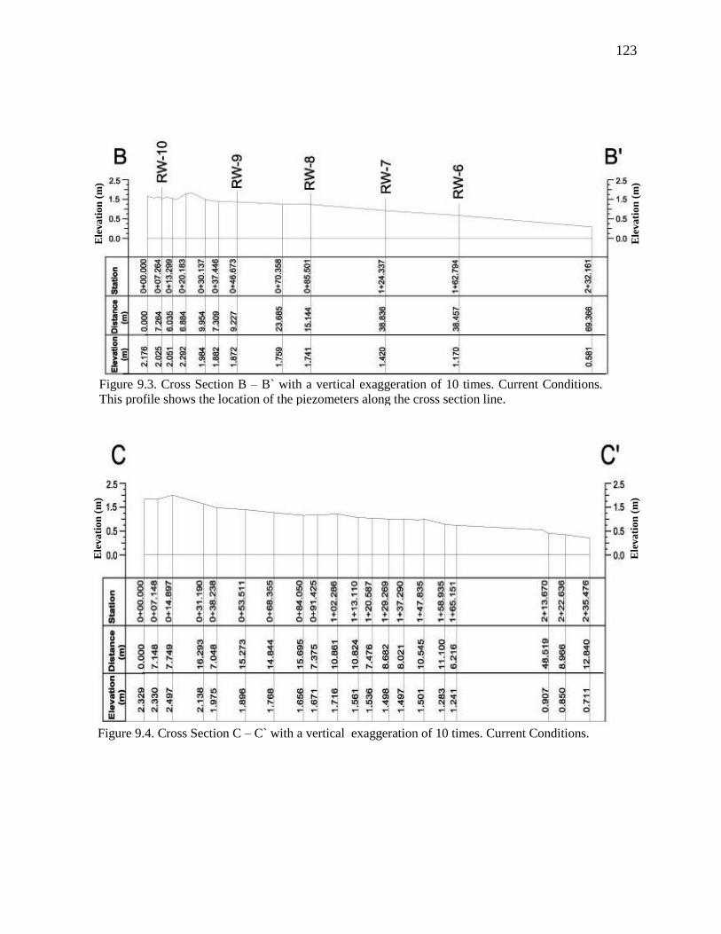
123
Ele
vati
on
(m
)
Figure 9.4. Cross Section C – C` with a vertical exaggeration of 10 times. Current Conditions.
Ele
vati
on
(m
)
Ele
vati
on
(m
)
Figure 9.3. Cross Section B – B` with a vertical exaggeration of 10 times. Current Conditions.
This profile shows the location of the piezometers along the cross section line.
Ele
vati
on
(m
)
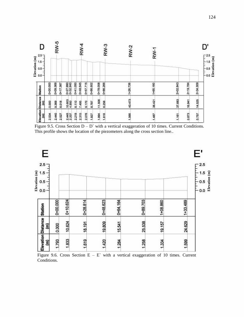
124
Figure 9.6. Cross Section E – E` with a vertical exaggeration of 10 times. Current
Conditions.
Ele
vati
on
(m
)
Ele
vati
on
(m
)
Figure 9.5. Cross Section D – D` with a vertical exaggeration of 10 times. Current Conditions.
This profile shows the location of the piezometers along the cross section line..
Ele
vati
on
(m
)
Ele
vati
on
(m
)

125
The calculation of cut and fill was prepared using AutoCAD. The area of cut or fill for
each cross section was calculated directly by the software and the distance between profiles was
measured directly from the cross sections lines (Figure 9.8). The tables of cut and fill results will
be shown after each cross-section set.
On the result tables, station values referred to Figure 9.9 which value 0+00 starts in the
first line (top) and increases down by 20 meters per line. Each cut and fill analysis will be
considering two contiguous profiles.
The cross sections B (Figure 9.10) and D (Figure 9.12), includes the location of the
piezometers structures. These piezometers contain a concrete base, which is part of the surface
seal of the structure, and serve as datum of the pipe surface elevation. If some excavation is
planned on this region, this area has to be protected and possible make a buffer zone to let some
room for safety and do not damage these structures.
9.2 CUT AND FILL
Figure 9.7. Cross Section I – I` with a vertical exaggeration of 10 times. Current Conditions.
This cross section represents the area to build the hydraulic design.
Ele
vati
on
(m
)
Ele
vati
on
(m
)
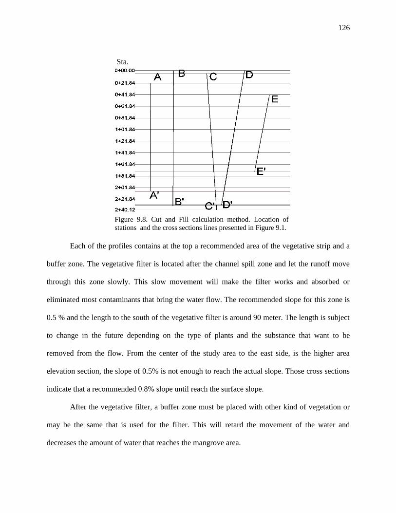
126
Each of the profiles contains at the top a recommended area of the vegetative strip and a
buffer zone. The vegetative filter is located after the channel spill zone and let the runoff move
through this zone slowly. This slow movement will make the filter works and absorbed or
eliminated most contaminants that bring the water flow. The recommended slope for this zone is
0.5 % and the length to the south of the vegetative filter is around 90 meter. The length is subject
to change in the future depending on the type of plants and the substance that want to be
removed from the flow. From the center of the study area to the east side, is the higher area
elevation section, the slope of 0.5% is not enough to reach the actual slope. Those cross sections
indicate that a recommended 0.8% slope until reach the surface slope.
After the vegetative filter, a buffer zone must be placed with other kind of vegetation or
may be the same that is used for the filter. This will retard the movement of the water and
decreases the amount of water that reaches the mangrove area.
Figure 9.8. Cut and Fill calculation method. Location of
stations and the cross sections lines presented in Figure 9.1.
Sta.
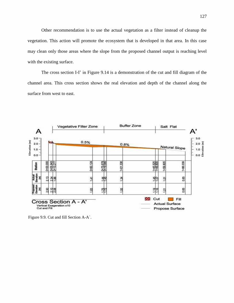
127
Other recommendation is to use the actual vegetation as a filter instead of cleanup the
vegetation. This action will promote the ecosystem that is developed in that area. In this case
may clean only those areas where the slope from the proposed channel output is reaching level
with the existing surface.
The cross section I-I’ in Figure 9.14 is a demonstration of the cut and fill diagram of the
channel area. This cross section shows the real elevation and depth of the channel along the
surface from west to east.
Figure 9.9. Cut and fill Section A-A`.
Ele
va
tio
n (
m)
Ele
va
tio
n (
m)
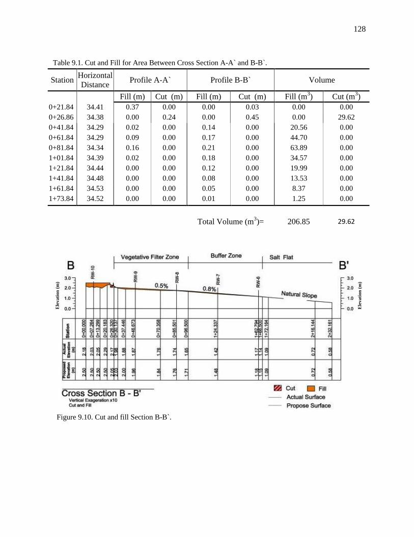
128
Station Horizontal
Distance Profile A-A` Profile B-B` Volume
Fill (m) Cut (m) Fill (m) Cut (m) Fill (m3) Cut (m
3)
0+21.84 34.41 0.37 0.00 0.00 0.03 0.00 0.00
0+26.86 34.38 0.00 0.24 0.00 0.45 0.00 29.62
0+41.84 34.29 0.02 0.00 0.14 0.00 20.56 0.00
0+61.84 34.29 0.09 0.00 0.17 0.00 44.70 0.00
0+81.84 34.34 0.16 0.00 0.21 0.00 63.89 0.00
1+01.84 34.39 0.02 0.00 0.18 0.00 34.57 0.00
1+21.84 34.44 0.00 0.00 0.12 0.00 19.99 0.00
1+41.84 34.48 0.00 0.00 0.08 0.00 13.53 0.00
1+61.84 34.53 0.00 0.00 0.05 0.00 8.37 0.00
1+73.84 34.52 0.00 0.00 0.01 0.00 1.25 0.00
Total Volume (m3)= 206.85 29.62
Table 9.1. Cut and Fill for Area Between Cross Section A-A` and B-B`.
Figure 9.10. Cut and fill Section B-B`.
Ele
va
tio
n (
m)
Ele
va
tio
n (
m)
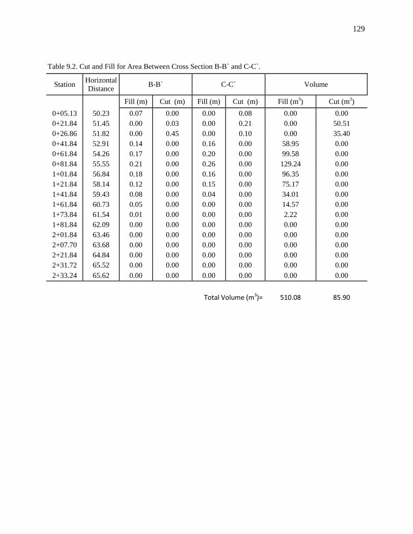
129
Station Horizontal
Distance B-B` C-C` Volume
Fill (m) Cut (m) Fill (m) Cut (m) Fill (m
3) Cut (m
3)
0+05.13 50.23 0.07 0.00 0.00 0.08 0.00 0.00
0+21.84 51.45 0.00 0.03 0.00 0.21 0.00 50.51
0+26.86 51.82 0.00 0.45 0.00 0.10 0.00 35.40
0+41.84 52.91 0.14 0.00 0.16 0.00 58.95 0.00
0+61.84 54.26 0.17 0.00 0.20 0.00 99.58 0.00
0+81.84 55.55 0.21 0.00 0.26 0.00 129.24 0.00
1+01.84 56.84 0.18 0.00 0.16 0.00 96.35 0.00
1+21.84 58.14 0.12 0.00 0.15 0.00 75.17 0.00
1+41.84 59.43 0.08 0.00 0.04 0.00 34.01 0.00
1+61.84 60.73 0.05 0.00 0.00 0.00 14.57 0.00
1+73.84 61.54 0.01 0.00 0.00 0.00 2.22 0.00
1+81.84 62.09 0.00 0.00 0.00 0.00 0.00 0.00
2+01.84 63.46 0.00 0.00 0.00 0.00 0.00 0.00
2+07.70 63.68 0.00 0.00 0.00 0.00 0.00 0.00
2+21.84 64.84 0.00 0.00 0.00 0.00 0.00 0.00
2+31.72 65.52 0.00 0.00 0.00 0.00 0.00 0.00
2+33.24 65.62 0.00 0.00 0.00 0.00 0.00 0.00
Total Volume (m3)= 510.08 85.90
Table 9.2. Cut and Fill for Area Between Cross Section B-B` and C-C`.
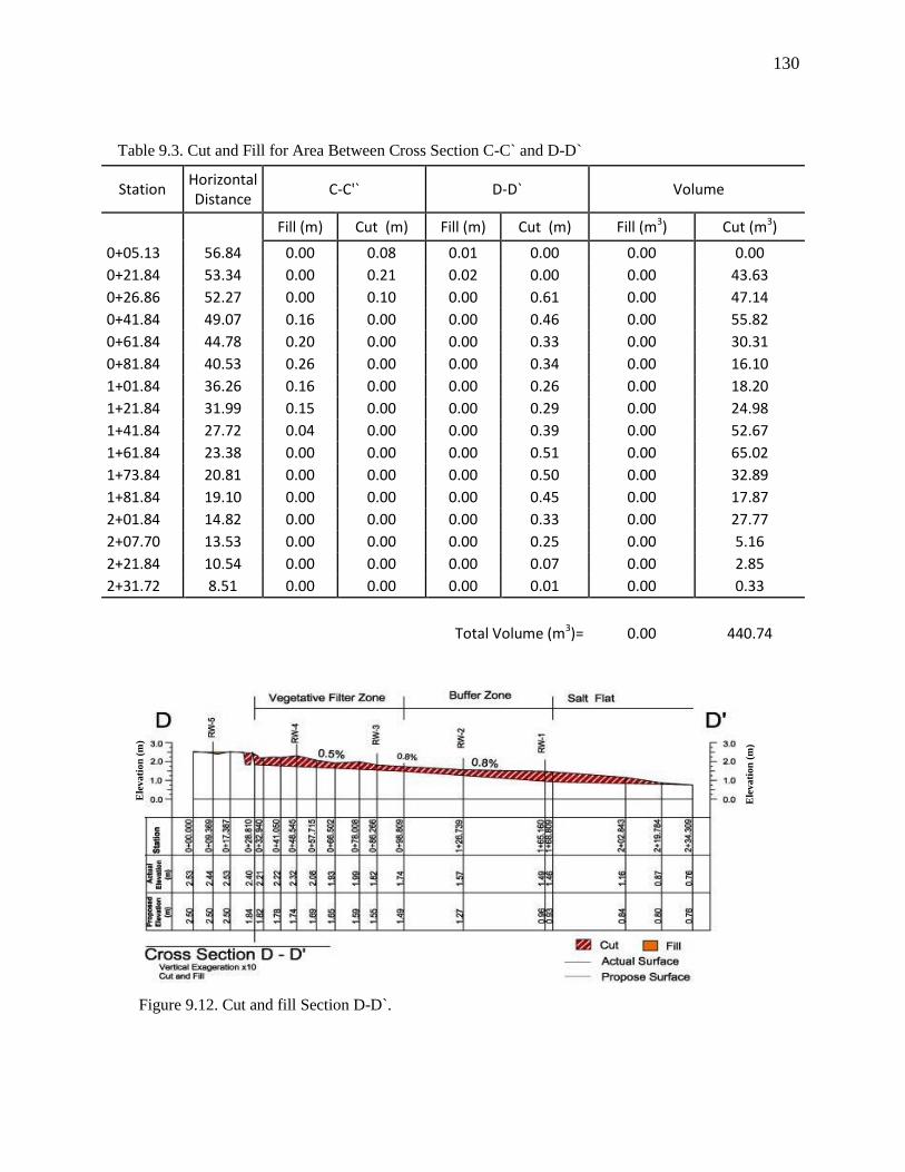
130
Table 9.3. Cut and Fill for Area Between Cross Section C-C` and D-D`
Station Horizontal Distance
C-C'` D-D` Volume
Fill (m) Cut (m) Fill (m) Cut (m) Fill (m3) Cut (m3)
0+05.13 56.84 0.00 0.08 0.01 0.00 0.00 0.00
0+21.84 53.34 0.00 0.21 0.02 0.00 0.00 43.63
0+26.86 52.27 0.00 0.10 0.00 0.61 0.00 47.14
0+41.84 49.07 0.16 0.00 0.00 0.46 0.00 55.82
0+61.84 44.78 0.20 0.00 0.00 0.33 0.00 30.31
0+81.84 40.53 0.26 0.00 0.00 0.34 0.00 16.10
1+01.84 36.26 0.16 0.00 0.00 0.26 0.00 18.20
1+21.84 31.99 0.15 0.00 0.00 0.29 0.00 24.98
1+41.84 27.72 0.04 0.00 0.00 0.39 0.00 52.67
1+61.84 23.38 0.00 0.00 0.00 0.51 0.00 65.02
1+73.84 20.81 0.00 0.00 0.00 0.50 0.00 32.89
1+81.84 19.10 0.00 0.00 0.00 0.45 0.00 17.87
2+01.84 14.82 0.00 0.00 0.00 0.33 0.00 27.77
2+07.70 13.53 0.00 0.00 0.00 0.25 0.00 5.16
2+21.84 10.54 0.00 0.00 0.00 0.07 0.00 2.85
2+31.72 8.51 0.00 0.00 0.00 0.01 0.00 0.33
Total Volume (m3)= 0.00 440.74
Figure 9.12. Cut and fill Section D-D`.
Ele
va
tio
n (
m)
Ele
va
tio
n (
m)
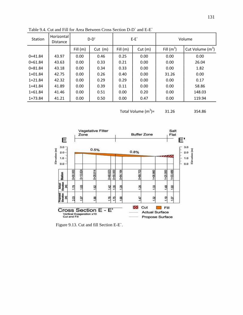
131
Station Horizontal Distance
D-D' E-E` Volume
Fill (m) Cut (m) Fill (m) Cut (m) Fill (m3) Cut Volume (m3)
0+41.84 43.97 0.00 0.46 0.25 0.00 0.00 0.00
0+61.84 43.63 0.00 0.33 0.21 0.00 0.00 26.04
0+81.84 43.18 0.00 0.34 0.33 0.00 0.00 1.82
1+01.84 42.75 0.00 0.26 0.40 0.00 31.26 0.00
1+21.84 42.32 0.00 0.29 0.29 0.00 0.00 0.17
1+41.84 41.89 0.00 0.39 0.11 0.00 0.00 58.86
1+61.84 41.46 0.00 0.51 0.00 0.20 0.00 148.03
1+73.84 41.21 0.00 0.50 0.00 0.47 0.00 119.94
Total Volume (m3)= 31.26 354.86
Table 9.4. Cut and Fill for Area Between Cross Section D-D` and E-E`
Figure 9.13. Cut and fill Section E-E`.
Ele
va
tio
n (
m)
Ele
va
tio
n (
m)
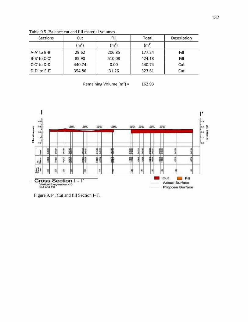
132
Table 9.5. Balance cut and fill material volumes.
Sections Cut Fill Total Description
(m3) (m3) (m3)
A-A' to B-B' 29.62 206.85 177.24 Fill
B-B' to C-C' 85.90 510.08 424.18 Fill
C-C' to D-D' 440.74 0.00 440.74 Cut
D-D' to E-E' 354.86 31.26 323.61 Cut
Remaining Volume (m3) = 162.93
.
Figure 9.14. Cut and fill Section I–I`.
Ele
va
tio
n (
m)
Ele
va
tio
n (
m)

133
The cost estimate is an approximation of the cost of a project. On this case, the
cost estimate is only related to the construction of the designed channel. Table 9.6 shows the cost
estimate of the grouted riprap channel. The unit price of the grouted riprap is $86.00 per cubic
yard (Cy) and includes the labor and materials (RS Means, etal., 2004). This cost estimate does
not include equipment, machinery or additional labor for the construction of the channel.
The walls cost computation was divided in the two individual channels (West; East) in
which the volumes consider the length of the wall (0.72; 1.4m), the width (0.20 m, see Table 5.2)
and the length of the channels (92m). The width of the bottom bed varies along the channel and
that is why the table shows 4 divisions of the channel. The minimum toe or bed for the channel
was 0.30 m (see Table 5.2) and this value was used to compute the area of the lining toe. Table
9.7 shows the same exercise but with reinforced concrete. This option was not used in the
project, but for comparison purpose was included in this section. For reinforced concrete, the toe
thicknesses as the walls are 0.15m. For volume computation this value was used in the equation.
The unit price for walls is $650 yd3 and $550 yd
3 cubic for the toe. This value includes
materials and labor for construction. The extended price for the reinforcement concrete resulted
ten times higher than the riprap. The grouted lining has a cost of around $19,000 and reinforces
concrete $80,000. Table 9.8 shows the complete conceptual cost estimate of the project. This
table includes the operational cost of the machinery leasing (considering the wage of the machine
operator and one helper), materials and labor necessary for the excavation process. The total cost
of this part is around $12,000 dollars for one working day. All this information about the
machinery cost and labor were taken from the software National Estimator 32 Pro (Craftsman
Book Company, 2013).
9.3 COST ESTIMATE
134
The total cost of the project is approximately $45,600 including the material, labor, 35%
of overhead and 15% of profit. This cost analysis does not include the transportation of the
machinery or materials to the site area. The existing vegetation at the south boundary of the
proposed channel, serves as a natural filter for overland flows. This natural filter could help to
improve the water quality promoting infiltration before reaching the mangrove area. A new
research is recommended to determine which species of plants can promote infiltration and
adsorption of pollutants found in previous investigations. If the new project involves the
replacement of vegetation, the existing vegetation should be cleared and a new grading should be
designed to produce better runoff. To improve the slope of the area is necessary a process of cut
and fill, as recommended in the previous section. This process can increase the total project cost
to around $ 60,000 (see Table 9.9).
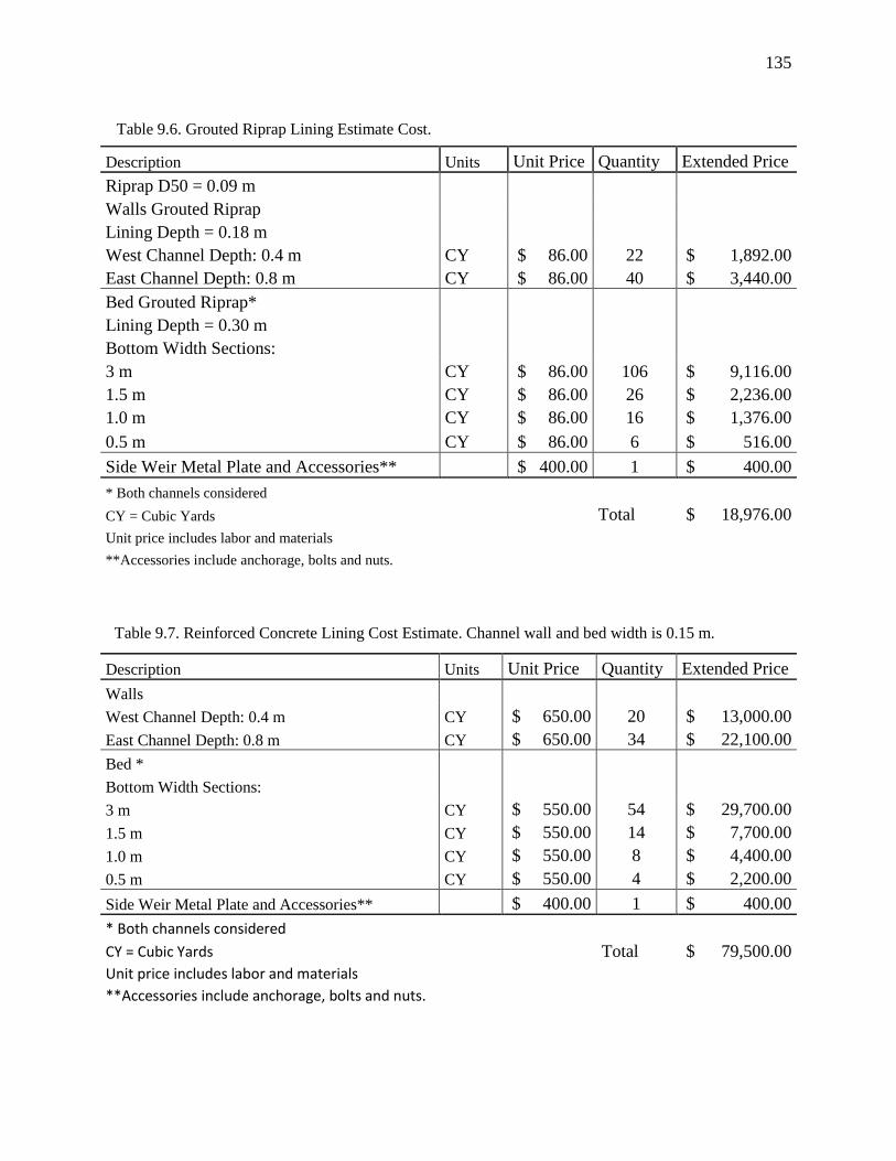
135
Table 9.6. Grouted Riprap Lining Estimate Cost.
Table 9.7. Reinforced Concrete Lining Cost Estimate. Channel wall and bed width is 0.15 m.
Description Units Unit Price Quantity Extended Price
Riprap D50 = 0.09 m
Walls Grouted Riprap
Lining Depth = 0.18 m
West Channel Depth: 0.4 m CY $ 86.00 22 $ 1,892.00
East Channel Depth: 0.8 m CY $ 86.00 40 $ 3,440.00
Bed Grouted Riprap*
Lining Depth = 0.30 m
Bottom Width Sections:
3 m CY $ 86.00 106 $ 9,116.00
1.5 m CY $ 86.00 26 $ 2,236.00
1.0 m CY $ 86.00 16 $ 1,376.00
0.5 m CY $ 86.00 6 $ 516.00
Side Weir Metal Plate and Accessories** $ 400.00 1 $ 400.00
* Both channels considered
CY = Cubic Yards
Total $ 18,976.00
Unit price includes labor and materials
**Accessories include anchorage, bolts and nuts.
Description Units Unit Price Quantity Extended Price
Walls
West Channel Depth: 0.4 m CY $ 650.00 20 $ 13,000.00
East Channel Depth: 0.8 m CY $ 650.00 34 $ 22,100.00
Bed *
Bottom Width Sections:
3 m CY $ 550.00 54 $ 29,700.00
1.5 m CY $ 550.00 14 $ 7,700.00
1.0 m CY $ 550.00 8 $ 4,400.00
0.5 m CY $ 550.00 4 $ 2,200.00
Side Weir Metal Plate and Accessories** $ 400.00 1 $ 400.00
* Both channels considered CY = Cubic Yards
Total $ 79,500.00
Unit price includes labor and materials **Accessories include anchorage, bolts and nuts.
136

137
138
BIBLIOGRAPHY
3001, Inc. (2007). Islans, Orthophoto Production in Puerto Rico and Adjacent. Peachtree City,
GA: U.S. Army Corpos Of Engineers.
Akan, A. O. (2006). Open Channel Hydraulics. Burlington, MA: Butterworth-Hainemann.
Anderson, A. G., Paintal, A. S., & Davenport, J. T. (1970). Tentative Design Procedure For
RipRap-Lined Channels. National Cooperative Highway Research Program, Federal Highway
Administration. Washington, D.C.: Federal Highway Administration.
Bagchi, A. (2004). Design of Landfills and Integrated Solid Waste Management. Hoboken, NJ:
John Wiley and Sons, Inc.
Bedient, P. B., Huber, W. C., & Vieux, B. E. (2008). Hydrology and Floodplain Analysis (fourth
Edition ed.). Upper Saddle River: Pearson, Prentice Hall.
Blanckaert, K., & De Vriend, H. J. (2004). Secondary flow in sharp open-channel bends. Journal
of Fluid Mechanics, 498, 353-380.
Chaudry, H. M. (2008). Open-Channel Flow (Second Edition ed.). New York, NY: Springer
Science+Business Media, LLC.
Cherry, G. S. (2001). Simulation of Flow in the Upper North Coast Limestone Aquifer, Manatí-
Vega Baja Area, Puerto Rico. San Juan, PR: USGS.
CHI. (2011). PCSWWM. Retrieved 2011, from CHI: http://www.chiwater.com/Software
/PCSWMM.NET/index.asp
Chow, V. T. (1959). Open-Channel Hydraulics. Caldwell, NJ: McGraw Hill Book Company,
Inc.
City of EL Paso, Engineering Department. (2008). Drainage Design Manual. El Paso, TX: The
City of el Paso.
Craftsman Book Company. (2013, November 5). 2014 National Construction Estimator.
Retrieved Novermer 5, 2013, from Craftsman Book Company: http://craftsman-book.com/
Demopoulos, A. W. (2004). Black Mangrove Benthic Community Structure , Seedling Groth and
Survival, and Sediment Characteristics in Anthropogenically Disturbed and Pristine Habitats.
Jobos Bay National Estuarine Research Reserve. Jobos Bay National Estuarine Research
Reserve.
Dieppa, A., Field, R., Laboy, E. N., Capellla, J., Robles, P. O., & González, C. O. (2008). Jobos
Bay Estuarine Profile, A National Estuarine Research Reserve. Aguirre: Jobos Bay NER.
139
Eftekharzadeh, S. (1985). Canal Side Weirs for Water Delivery to Irrigation Furrows. Sierra
Vista, Az.: The University of Arizona.
Eijkelkamp Agrisearch Equipment. (1999). Operating Instructions 09-04 Double Ring
Infiltrometer Set. Giesbeek, NL: Eijkelkamp Agrisearch Equipment.
Emiroglu, M., Agaccioglu, H., & Kayaa, N. (2011, August). Discharging capacity of rectangular
side weirs in straight open channels (Vol. 22). ELSEVIER.
Engman, E. T. (1986). Roughness Coefficients for Routing Surface Runoff. Journal of Irrigation
and Drainage Engineering., 112, 39-53.
Environmental Protection Agency. (2013, February 1). Storm Water Management Model
(SWMM). Retrieved from http://www.epa.gov/nrmrl/wswrd/wq/models/swmm/
Federal Highway Administration. (1988). Open Channel Hydraulics. Federal Highway
Administration.
Federal Highway Administration. (2012, 8 29). Hydraulics Engineering. (V. Ghelardi, Editor, &
U.S. Department of Transportation) Retrieved 2 12, 2013, from Introduction to Highway
Hydraulics - Chapter 4 - Open-Channel Flow: http://www.fhwa.dot.gov/engineering/hydraulic
s/pubs/08090/04.cfm
French, R. H. (1987). Open-Channel Hydraulics. (J. Z. Margolies, Ed.) New York: MacGraw-
Hill Book Co.
Garber, N. J., & Hoel, L. A. (2002). Traffic and Highway Engineering (Third Edition ed.).
Pacific Grove, CA: Brooks Cole.
Garcia, M. H. (2007). Sedimentation engineering: processes, measurements, modeling, and
practice. Reston, VA: American Society of Civil Engineers.
Ghere, D. (2011). Design of Roadside Channels with Flexible Linings. In F. H. Administration,
Hydraulic Engineering Circular Number 15, Third Edition. Federal Highway Administration.
Glover, L. (1961). Preliminary Geologic Map of the Salinas Quadrangle. U.S. Geological
Survey. U.S. Geological Survey.
Gonzalez, C. M. (2010). Jobos Bay National Estuarine Research Reserve Management Plan
Final 2010-2015. Puerto Rico Department of Natural and Environmental Resource. Aguirre, PR:
Puerto Rico Department of Natural and Environmental Resource.
Graves, R. P. (1992). Geohydrology of the Aguirre and Pozo Hondo Areas, Southern Puerto
Rico. US Geological Surviey. San Juan, P.R.: US Geological Survey.
Gregory L. Morris & Associates. (2000). Hydrologic-Hyraulic and Biological Analysis of Jobos
Estuary Mangrove Mortality Jobos, Puerto Rico. Santurce, P.R.: Puerto Rico Land Authority.
140
Hager, W. H., & ASCE, M. (1986). Lateral Outflow Over Side Weirs. 113. Journal of Hydraulic
Engineering,.
Henderson, F. M. (1966). Open Channel Flow. New York, NY: Macmillan Publishing Comp.,
Inc.
Ippen, A. T., & Drinker, P. A. (1961). Boundary Shear Stresses in Curved Trapezoidal
Channels. Cambridge, MA: Massachustts Institute of Technology.
James, R., James, W., Finney, K., & Lee, M. (2012, January 12). Urban Drainage Modeling
Workbook. CHI Press R231. Guelp, Ontario, Canada: Computational Hydraulics International.
James, W., & James, R. C. (2000). Water System Models Hydrology, A guide to the Rain,
Temperature and Runoff Models of the USEPA Swmm4. Canada: Computational Hydraulics
International.
James, W., Rossman , L. E., & James, W. C. (2011). Water System Models, User`Guise to
SWMM5 (13th Edition ed.). Ontario, Canada: Computational Hydraulics International.
Ka-Leung, L., & Holley, E. (2002). Physical Modeling For Side Channel Weirs. The University
of Texas at Austin, Harris Flood Control District, TX. Austin, TX.: Center for Research in Water
Resources.
Kuniansky, E. L., & Rodríguez, J. M. (2010). Effects of Changes in Irrigation Practices and
Aquifer Development on Groundwater Discharge to the Jobos Bay National Estuarine Research
Reserve near Salinas, Puerto RicoBy. U.S. Geological Survey.
Maidment, D. R. (1992). Handbook of Hydrology. New York: McGraw-Hill Inc.
May, R., Bromwich, B., Gasowski, Y., & Rickard, C. (2003). Hydraulic Design of Side Wiers.
Reston, VA: Thomas Telford Publishing.
Mays, L. W. (2005). Water Resources Engineering (2005 Edition ed.). Hoboken, NJ, NJ:
Hamilton Printing Company.
Miller, J. F. (1965). Two- to Ten-Day Rainfall for Return Periods of 2 to 100 Years in Puerto
Rico and Virgin Islands. Weather Bureau, Department of Comerce. Washington D.C.: U.S.
Goverment Printing Office.
Mockus, V. (2004). Hydrologic Soil over Complexes. In N. R. Service, Part 630, National
Engineering Handbook. Beltsville, MA: U. S. Departemn of Agriculture.
Mohan Das, M., & Das Saikia, M. (2009). Hydrology. Connaught Circus, New Dejlhi: Asoke K.
Ghosh, PHI Learning Limited.
National Climatic Data Center (NCDC). (2010). NOAA Satellite and Information Service.
Retrieved February 12, 2012, from www.ncdc.noaa.gov/oa/climate/stationlocator.html
141
National Estuarine Research Reserve System. (2012). 0.1. Retrieved January 7, 2012, from
Centralize Data Management Office: http://cdmo.baruch.sc.edu/get/gisapp.cfm?fileType=
Shapefile
National Oceanic and Atmospheric Administration (NOAA). (2010). National Climate Data
Center. Retrieved January 2011, from Climate Data Online: http://www.ncdc.noaa.gov/cdo-
web/search
National Weather Service Weather Forecast Office. (2009, April 29). San Juan. Retrieved
January 17, 2012, from Puerto Rico Mean Annual Presipitation 1971-2000 : http://www.srh.
noaa.gov/sju/?n=mean_annual_precipitation
Natural Resources Conservation Service. (2011, 11 20). Custom Soil Resource Report for
Humacao Area, Puerto Rico Eastern. Retrieved from http://websoilsurvey.nrcs.usda.gov
/app/websoilsurvey.aspx
Natural Resources Conservation Service Caribbean Area. (2012, August 7). Saltflat Vegetation
for Soil and Wildlife Conservation Associated with Coastal Tidal Flats. ( Cooperative Agreement
# 68-F352-09-02). NRCS Fact Sheet.
NOAA, Atlas 14. (2012, 12 3). Point Precipitation Frequency Estimates, Volume 3, Version 4 .
(N. N. Services, Producer) Retrieved 03 26, 2013, from Hydrometeorological Design Study
Center: http://hdsc.nws.noaa.gov/hdsc/pfds/pfds_printpage.html?lat=17.9529&lon=-66.2461&
data=depth&units=english&series=pds
NRCS. (1986). Urban Hydrology for Small watersheds (TR-55). Natural Resources Conservation
Service, U. S. Department of Agriculture. NRCS.
NRCS. (2009). Salinas Forage Farm Location; Puerto Rico, USA. (p. 41). Natural Resources
Conservation Service.
Ormsby, T., Napoleon, E., Burke, R., Groessl, C., & Bowden, L. (2009). Getting to Know
ArcGIS Desktop. New York: ESRI Press.
Quiñones-Aponte, V., Gómez-Gómez, F., & Renken, R. A. (1996). Geohydrology and
Simulation of Ground_Water Flow in the Salinas to Patillas Area, Puerto Rico. U.S. Geological
Survey, NOAA Technical Memorandum NOSNCCOS 76. San Juan, P.R.: U.S. Geological
Survey.
Rawis, W. J., Ahuja, L. R., Brakensiek, D. L., & Shirmohammadi, A. (1992). Infiltration and
Soil Water Movement. In D. R. Maidment, Handbook of Hydrology (pp. 5.0-5.46). New York,
New York, U.S.: MacGraw-Hill, Inc.
Renken, R. A., Ward, W., Gill, I., Gómez-Gómez, F., & Rodríguez-Martínez, J. (2002). Geology
and Hydrogeology of the Caribbean Islands Aquifer System of the Commonwealth of Puerto
Rico and the U.S. Virgin Islands. Reston, Virginia: U.S. Department of the Interior, U.S.
Geological Survey.
142
Rodríguez, J. M. (2006). Evaluation of Hydrologic Conditions and Nitrate Concentrations in the
Río Nigua de Salinas Alluvial Fan Aquifer, Salinas, Puerto Rico, 2002-03. U.S. Geological
Survey. Reston, VA: U.S. Geological Survey.
Roman Guzman, I. M. (2010). Estudio Comparativo Entre el Perfil Bacteriano de Sedimento de
Mangle en la Cienaga Cucharillas y Bahia de Jobos por Medio de la Tecnica "Termal Restriction
Fragment Length Polymorphism" (T-RFLP). San Juan: Universidad Metropolitana.
Rosier, B. (2007). Interaction of Side Weir Overflow With Bed-load Transport and Bed
Morphology in a Channel. Karlsruhe University, Civil Enginering. Switzerland: Ecole
Polytechnique, Federale de Lausanne.
Rosier, B., Boillat, J.-L., & J. Schleiss, A. (2008). Outflow angle for side weirs in a channel. (pp.
199-208). INTERPRAEVENT 2008 – Conference Proceedings, Vol. 1.
Rossman, L. A. (2010, July). Storm Water Management Model User`s Manual version 5.0.
Cincinnati, Ohio, U.S.: Water Supply and Water Resources Division.
Rowlings, D. S. (2010). An Experimental and Theorical Investigation of Side Weirs. University
of Southern Queensland.
RS Means, Barbara Balboni, Robert A. Bastoni. (2004). Building Construction Cost Data 2005
(63 ed.). Portland, OR: RS Means.
Soil Conservation Service. (2013, 2 15). Web Soil Survey. Retrieved 10 25, 2013, from USDA,
Natural Resources Conservation Service: http://websoilsurvey.nrcs.usda.gov/app/WebSoil
Survey.aspx
Sturm, T. W. (2011). Open Channel Hydraulics (Second ed.). New York, New York, U.S.:
McGraw-Hill Companies Inc.
Thompson, P. L., & Kilgore, R. T. (2006). Hydraulic Design of Energy Dissipators for Culverts
and Channels. Federal Highway Administration, U.S. Department of Transportation. Federal
Highway Administration.
Thornton, C. I., & Ursic, M. E. (2011). Quatification of Shear Stress in a Meandering Native
Topographic Channel Using a Physical Hydraulic Model. Fort Collins, Colorado: Colorado State
University.
Torres-Gonzales, S., Planert, M., & Rodriguez, J. M. (1996). Hydrogeology and Simulation of
Ground-Water Flow in the Upper Aquifer of the Rio Camuy to Rio Grande de Manati Area,
Puerto Rico . San Juan, PR: USGS.
U.S. Army Corps of Engineers (USACE). (1994). Hydraulic Design of Flood Control Channels,"
Engineering and Design Manual.
U.S. Department of Agriculture (USDA). (2004). Orthophoto Mosaic for Puerto Rico. Fort
Worth, TX: USDA, Natural Resources Conservation Service.
143
U.S. Geological Survey (USGS). (2006). National Elevation Dataset. Retrieved December 2011,
from EROS data Center: http://gisdata.usgs.net/ ned/
Veve, T. D., & Taggart, B. E. (1996). Atlas of Ground Water Resources in Puerto Rico and the
U. S. Virgin Islands. U.S. Geological Survey. San Juan, P.R.: U.S. Geological Survey.
Vidiani.com Maps of the World. (2011). Large detailed relief map of Puerto Rico. Retrieved
February 15, 2012, from http://www.vidiani.com/?p=6290
WEF and ASCE. (1992). Design and construction of Urban Stormwater Management Systemn.
Water Environment Federation (WEF) and American Society of Civil Engineers (ASCE).
Whitall, D. R., Costa, B. M., Bauer, L. J., Dieppa, A., & Hile, S. D. (2011). A Baseline
Assessment of the Ecological Resources of Jobos Bay, Puerto Rico. National Oceanic and
Atmospheric Administration, U.S. Department of Commerce. Silver Spring, MD: National
Oceanic and Atmospheric Administration.
Williams, C. O., Lowrance, R., Bosch, D. D., Williams, J. R., Benham, E., Dieppa, A., et al.
(2012, September 28). Hydrology and Water Quality of a Field and Riiparian Buffer Adjacent to
a Mangrove Wetland in Jobos Bay Watershed, Puerto Rico. Ecological Engineering(ECOENG-
2313;), 9.
Zitello, A. G., Whitall, D. R., Dieppa, A., Christensen, J. D., Monaco, M. E., & Rohman, S. O.
(2008). Characterizing Jobos Bay, Puerto Rico: A Watershed Modeling Analysis and Monitoring
Plan. National Oceanic and Atmospheric Administration, U.S. Department of Agriculture. Silver
Spring, MD: National Oceanic and Atmospheric Administration.

144
APPENDIX
Appendix A Curve Number Tables
Table A.1. Curve Number For hydrologic soil groups (NRCS, 1986).
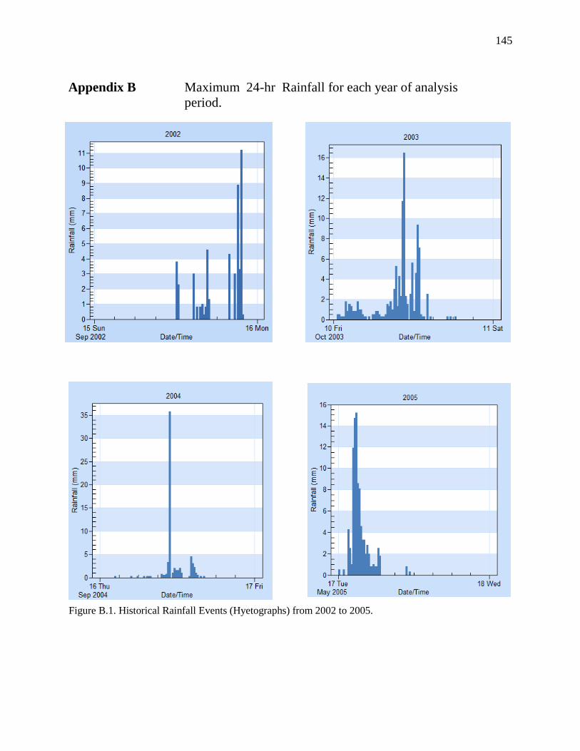
145
Appendix B Maximum 24-hr Rainfall for each year of analysis
period.
Figure B.1. Historical Rainfall Events (Hyetographs) from 2002 to 2005.
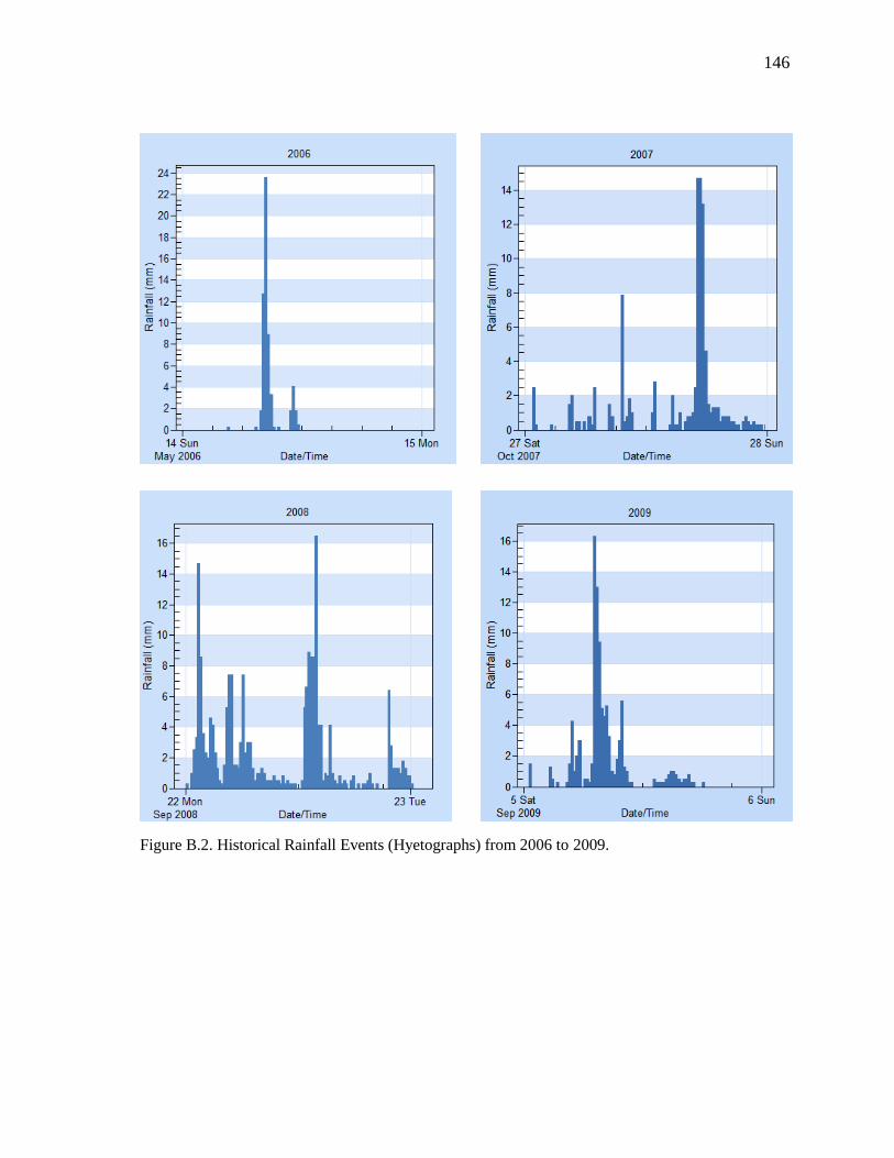
146
Figure B.2. Historical Rainfall Events (Hyetographs) from 2006 to 2009.

147
Figure B.3. Historical Rainfall Events (Hyetographs) from 2006 to 2009.
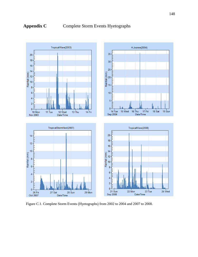
148
Appendix C Complete Storm Events Hyetographs
Figure C.1. Complete Storm Events (Hyetographs) from 2002 to 2004 and 2007 to 2008.
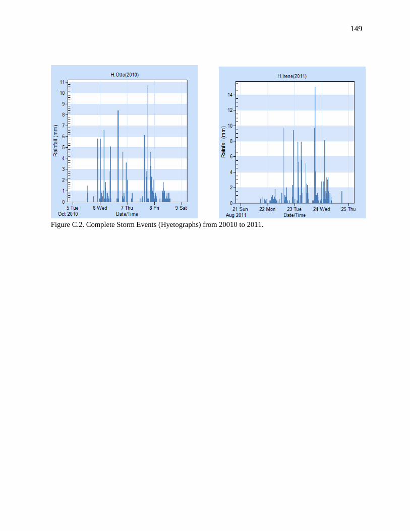
149
Figure C.2. Complete Storm Events (Hyetographs) from 20010 to 2011.
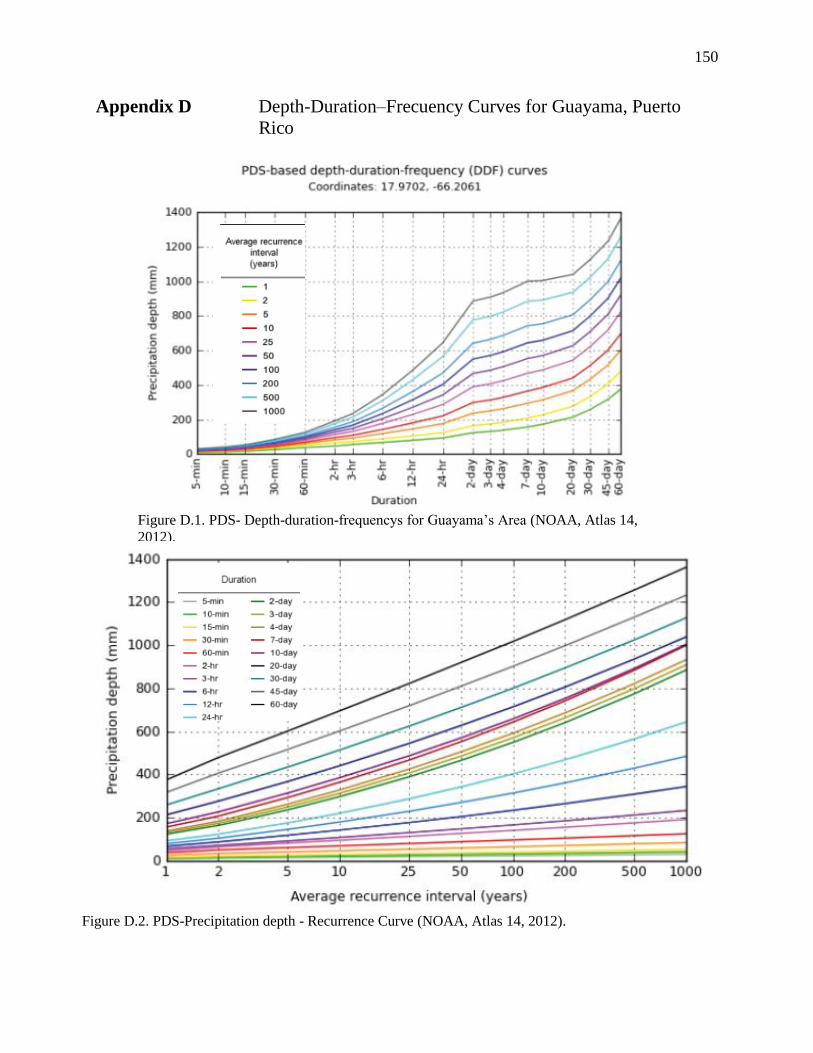
150
Figure D.2. PDS-Precipitation depth - Recurrence Curve (NOAA, Atlas 14, 2012).
Appendix D Depth-Duration–Frecuency Curves for Guayama, Puerto
Rico
Figure D.1. PDS- Depth-duration-frequencys for Guayama’s Area (NOAA, Atlas 14,
2012).
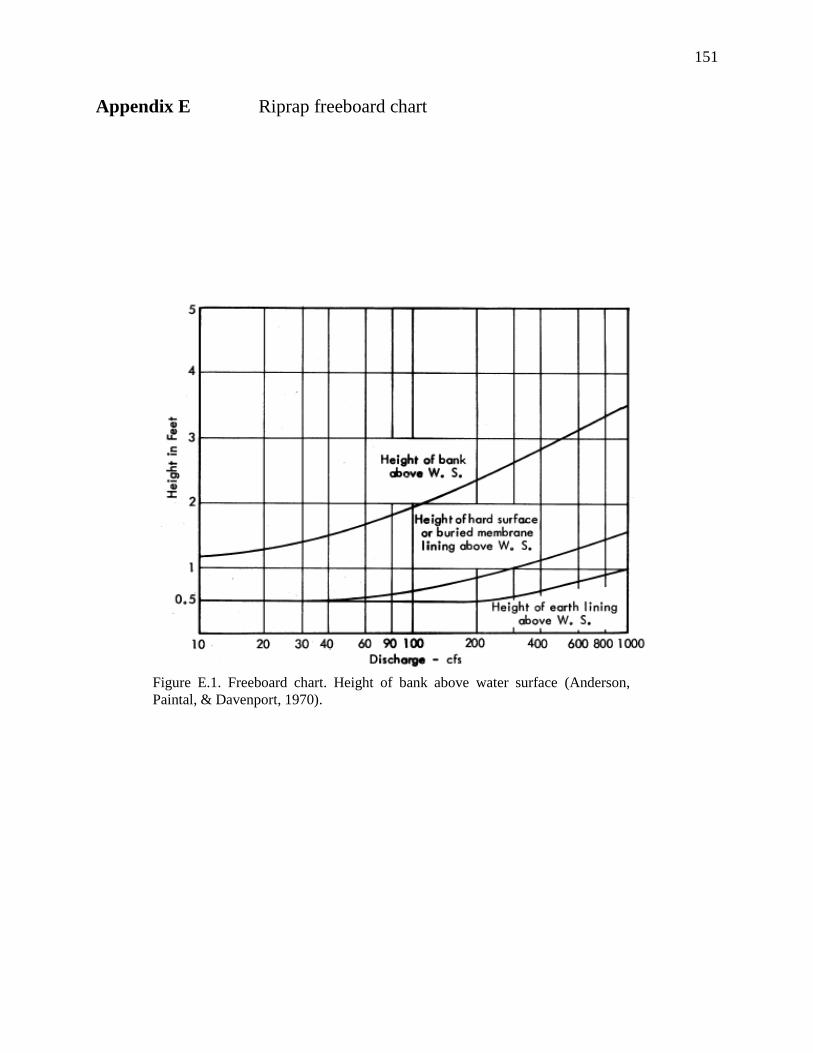
151
Appendix E Riprap freeboard chart
Figure E.1. Freeboard chart. Height of bank above water surface (Anderson,
Paintal, & Davenport, 1970).
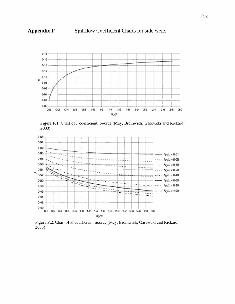
152
Appendix F Spillflow Coefficient Charts for side weirs
Figure F.1. Chart of J coefficient. Source (May, Bromwich, Gasowski and Rickard,
2003)
Figure F.2. Chart of K coefficient. Source (May, Bromwich, Gasowski and Rickard,
2003)

153
Appendix G Euler improved method for side weir water profile –
Excel VBA
Option Explicit
Sub ImprovedEuler2()
'Other variables:
'
'B = Channel Bottom Widht
'S= Channel Lateral Slope
'S0 = Channel Longitudina Slope
'MN = Channel Mannings Coef
'Q = Main Channel Discharge
'YD = Downstream Depht
'qweir = Weir Disch. per unit length
'N = Number of reaches for compilation
'L = Weir Length:
'G = Accel of Gravity
'Alpha = Kinetic Energy Coef
'A = Area
'R = Hydraulic radius
'Sf = Friction slope
Dim X(100) As Single, YY(100) As Single, Y As Single, B0 As Single, S As Single
Dim SO As Single, MN As Single, Q As Single, YD As Single, qweir As Single, N As Integer
Dim L As Single, G As Single, Alpha As Single, Cman As Single, DX As Single
Dim A As Single, P As Single, R As Single, I As Integer, SF1 As Single, Sf2 As Single
Dim B As Single, Num1 As Single, Num2 As Single, Den1 As Single, Den2 As Single
Dim DY1 As Single, DY2 As Single, Y2 As Single
With Worksheets("WDesign").Range("J30")
Range(.Offset(1, 0), .End(xlDown).End(xlToRight)).ClearContents
End With
`Variable calls from excel
B0 = Range("I17")
S = Range("I18")
SO = Range("I19")
MN = Range("I20")
Q = Range("I21")
YD = Range("I22")
qweir = Range("I23")
N = Range("I24")
L = Range("I25")
G = Range("I26")
154
'Computations
Alpha = Range("I27")
Cman = 1
Worksheets("WDesign").Range("H31") = "Problem in International Units"
If G > 12 Then
Cman = 1.49
Worksheets("WDesign").Range("H31") = "Problem in English Units"
End If
Y = YD
DX = -L / N
For I = 1 To N
A = Y * (B0 + S * Y)
P = B0 + 2 * Y * Sqr(1 + S * S)
R = A / P
If I = 1 Then
Worksheets("WDesign").Range("I31").Offset(0, 1) = 0 'offset produce un movimiento hacia la
izquierda en cada iteraccion
Worksheets("WDesign").Range("I31").Offset(0, 2) = Y
Worksheets("WDesign").Range("I31").Offset(0, 3) = Q
Worksheets("WDesign").Range("I31").Offset(0, 4) = qweir * Abs(X(I))
Worksheets("WDesign").Range("I31").Offset(0, 5) = Y * (B0 + S * Y)
Worksheets("WDesign").Range("I31").Offset(0, 6) = B0 + 2 * Y * Sqr(1 + S * S)
Worksheets("WDesign").Range("I31").Offset(0, 7) = (Y * (B0 + S * Y)) / (B0 + 2 * Y * Sqr(1 +
S * S))
End If
' Downstream
SF1 = (MN * Q) ^ 2 / (A * A * R ^ (4 / 3) * Cman ^ 2) ' Friction loss downstream
B = B0 + 2 * S * Y
Num1 = SO - SF1 - (Alpha * qweir * Q) / (G * A ^ 2) ' numerator of the Gradually Varied flow
equation
Den1 = 1 - ((B * Q * Q * Alpha) / (G * A ^ 3)) ' denominator of the Gradually Varied flow
equation
DY1 = Num1 / Den1 ' Gradually Varied Flow equation
'upstream
Y2 = Y + DY1 * DX ' Change in Depth - moving upstream
A = Y2 * (B0 + S * Y2) ' Area Upstream
P = B0 + 2 * Y2 * Sqr(1 + S * S)
R = A / P
Q = Q + qweir * Abs(DX) ' qweir is negative because is the substration of water (weir) from the
system
Sf2 = (MN * Q) ^ 2 / (A * A * R ^ (4 / 3) * Cman ^ 2) ' Friction loss upstream
B = B0 + 2 * S * Y2
Num2 = SO - Sf2 - (Alpha * qweir * Q) / (G * A ^ 2) 'dividend of the Gradually Varied Flow
equation
Den2 = 1 - (B * Q * Q * Alpha) / (G * A ^ 3) ' dividend of the Gradually Varied Flow equation

155
DY2 = Num2 / Den2
Y = Y + 0.5 * (DY1 + DY2) * DX
X(I) = I * DX
YY(I) = Y
Worksheets("WDesign").Range("I31").Offset(I, 1) = X(I)
Worksheets("WDesign").Range("I31").Offset(I, 2) = YY(I)
Worksheets("WDesign").Range("I31").Offset(I, 3) = Q
Worksheets("WDesign").Range("I31").Offset(I, 4) = qweir * Abs(X(I))
Worksheets("WDesign").Range("I31").Offset(I, 5) = YY(I) * (B0 + S * YY(I))
Worksheets("WDesign").Range("I31").Offset(I, 6) = B0 + 2 * YY(I) * Sqr(1 + S * S)
Worksheets("WDesign").Range("I31").Offset(I, 7) = (YY(I) * (B0 + S * YY(I))) / (B0 + 2 *
YY(I) * Sqr(1 + S * S))
Next I
End Sub
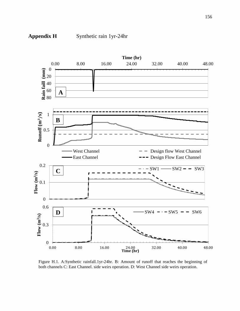
156
Appendix H Synthetic rain 1yr-24hr
0
20
40
60
80
0.00 8.00 16.00 24.00 32.00 40.00 48.00
Rain
fail
l (
mm
)
Time (hr)
0
0.5
1
Ru
no
ff (
m3/
s)
West Channel Design flow West Channel
East Channel Design Flow East Channel
0
0.3
0.6
0.00 8.00 16.00 24.00 32.00 40.00 48.00
Flo
w (
m3/s
)
Time (hr)
SW4 SW5 SW6
0
0.1
0.2
Flo
w (
m3/s
)
SW1 SW2 SW3
Figure H.1. A:Synthetic rainfall.1yr-24hr. B: Amount of runoff that reaches the beginning of
both channels C: East Channel. side weirs operation. D: West Channel side weirs operation.
A
B
C
D
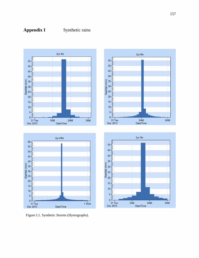
157
Appendix I Synthetic rains
Figure I.1. Synthetic Storms (Hyetographs).
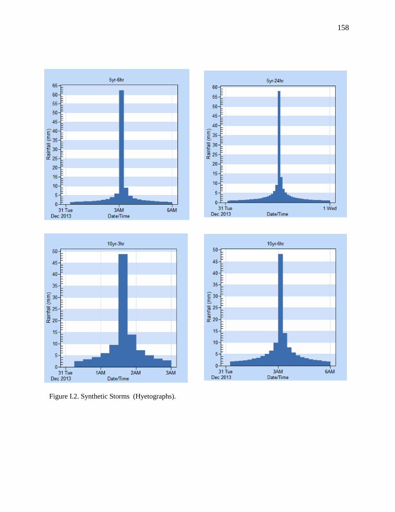
158
Figure I.2. Synthetic Storms (Hyetographs).

159
Figure I.3. Synthetic Storm (Hyetographs).
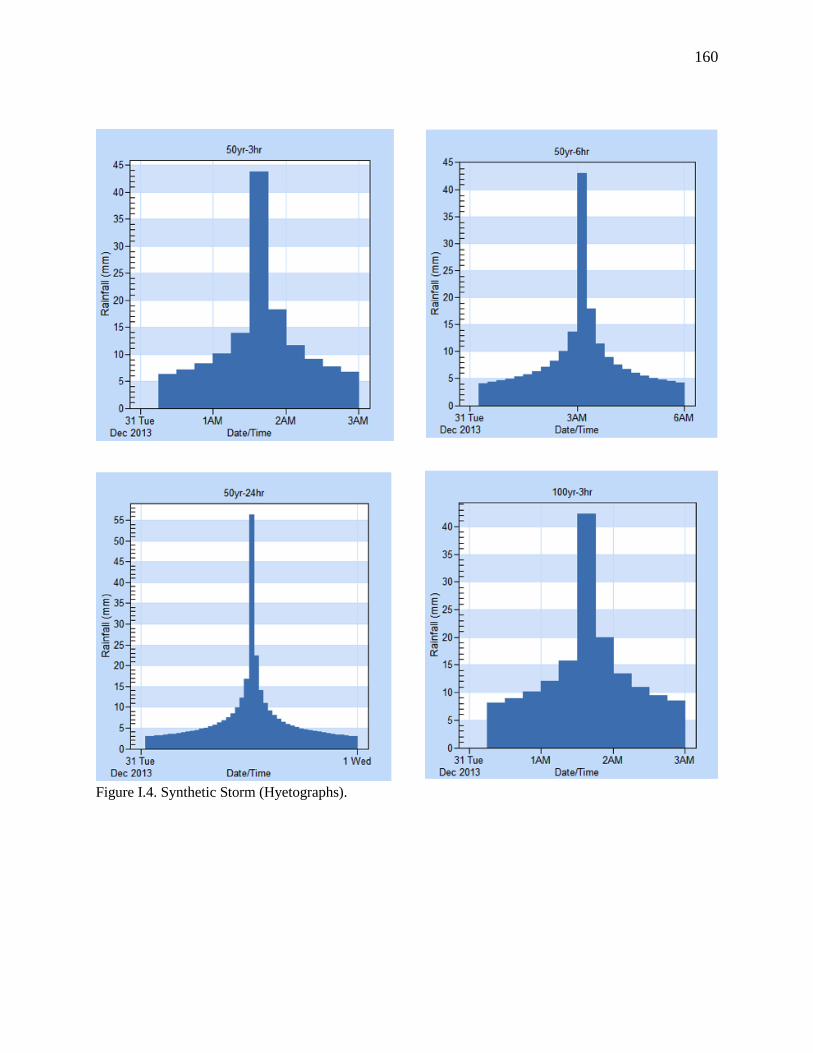
160
Figure I.4. Synthetic Storm (Hyetographs).
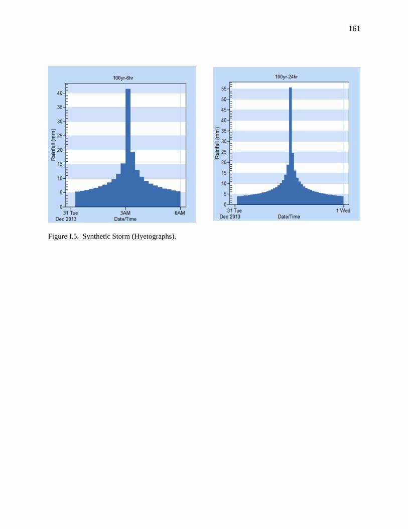
161
Figure I.5. Synthetic Storm (Hyetographs).

162
Appendix J Miscellaneous
VBA Hydraulic scripts
Variables
Y = Water depth
Ac = Area
R = Hydraulic radius
N = Roughness coefficient
Q = Flow
S0 = Longitudinal slope
m = Channel side slope
P = Wetted perimeter
fc = Function of Manning equation
ffc = First derivative of Manning Equation
Bc = Top width
frc = Function of Froude equation
ffrc = First derivative of Froude Equation
G = Aceleration by gravity
B = Bottom width
dyc = Counter limits precision
Range(“ “) = Location in excel where to call or save the value
Computation of Normal Depth
B = Range("C235").Value
Y = 0.0001
dyc = 0.0001
While Abs(dyc) > 0.000001
Ac = B * Y + m * Y ^ 2
Bc = B + 2 * m * Y
P = B + 2 * Y * (m ^ 2 + 1) ^ 0.5
R = Ac / P
fc = S0 ^ 0.5 * Ac * R ^ (2 / 3) / N - Q1

163
ffc = (S0 ^ 0.5 / N) * (R ^ (2 / 3) * Bc + Bc / P - (2 * Y * R / P))
Y = Y - fc / ffc
dyc = -fc / ffc
Wend
Range("C329").Value = Y
Computation of Critical Depth
ycd = 0.0001
dyc = 0.0001
While Abs(dyc) > 0.000001
Ac = B * ycd + m * ycd ^ 2
Bc = B + 2 * m * ycd
frc = Ac ^ (3 / 2) / (Bc ^ (1 / 2)) - Q1 / (G) ^ 0.5
ffrc = Ac ^ (3 / 2) * (-1 / 2) * Bc ^ (-3 / 2) * 2 * m + Bc ^ (-1 / 2) * (3 / 2) * Ac ^ (1 / 2) * Bc
ycd = ycd - fc / ffc
dyc = -frc / ffrc
Wend
Range("C328").Value = ycd
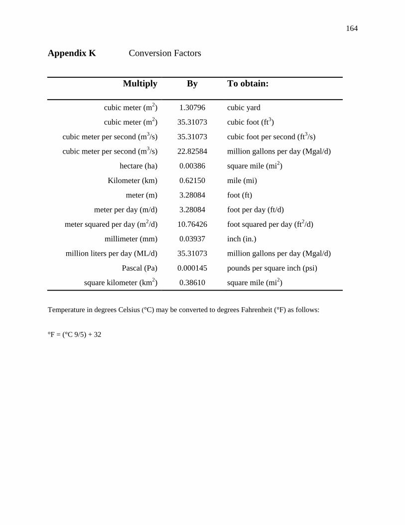
164
Appendix K Conversion Factors
Multiply By To obtain:
cubic meter (m2) 1.30796 cubic yard
cubic meter (m2) 35.31073 cubic foot (ft
3)
cubic meter per second (m3/s) 35.31073 cubic foot per second (ft
3/s)
cubic meter per second (m3/s) 22.82584 million gallons per day (Mgal/d)
hectare (ha) 0.00386 square mile (mi2)
Kilometer (km) 0.62150 mile (mi)
meter (m) 3.28084 foot (ft)
meter per day (m/d) 3.28084 foot per day (ft/d)
meter squared per day (m2/d) 10.76426 foot squared per day (ft
2/d)
millimeter (mm) 0.03937 inch (in.)
million liters per day (ML/d) 35.31073 million gallons per day (Mgal/d)
Pascal (Pa) 0.000145 pounds per square inch (psi)
square kilometer (km2) 0.38610 square mile (mi
2)
Temperature in degrees Celsius (°C) may be converted to degrees Fahrenheit (°F) as follows:
°F = (°C 9/5) + 32


