1
An-Najah National University Faculty of Graduate Studies
HYDRAULIC PERFORMANCE OF PALESTINIAN WATER DISTRIBUTION SYSTEMS
(JENIN WATER SUPPLY NETWORK AS A CASE STUDY)
Prepared by
Shaher Hussni Abdul Razaq Zyoud
Supervised by
Dr. Hafez Shaheen
Submitted in Partial Fulfillment of the Requirements for the Degree of Master of Water and Environmental Engineering, Faculty of Graduate Studies, at An-Najah National University, Nablus, Palestine.
2003

2
HYDRAULIC PERFORMANCE OF PALESTINIAN WATER DISTRIBUTION SYSTEMS
(JENIN WATER SUPPLY NETWORK AS A CASE STUDY)
Prepared by
Shaher Hussni Abdul Razaq Zyoud
This Thesis was defended successfully on 25 / 1 /2004 and approved by: Committee Members Signature 1 Dr. Hafez Shaheen --------------- Dept. of Civil Engineering, An-Najah National University 2 Dr. Anan Jayyousi --------------- Dept. of Civil Engineering, An-Najah National University 3 Dr. Issam AL-Khatib ---------------- Institute of Community and Public Health, Birzeit University

3
ACKNOWLEDGEMENTS
I wish to express my gratitude to my supervisor, Dr. Hafez Shaheen, for his efforts, useful suggestions, and encouragements, which provided valuable guidance. Also I would like to acknowledge the advice and assistance of Dr. Anan Jayyousi of An-Najah National University, and a specific gratitude is given to Dr. Isam AL-Khatib of Birzeit University. Specific gratitude is given to Eng. Abdel Fatah Rasem, at the Municipality of Jenin, for his valuable assistance; also specific recognition is given to Eng. Maher Abu Madi, Eng. Steffen Macke, Eng. Gada Al-Asmar for their valuable help. A special word of thanks is extended to my family, father; mother; brothers and sisters. Finally, I wish to thank all those who have helped me by one way or another during this research.

4
LIST OF CONTENTS
Acknowledgements I List of contents II List of tables VI List of figures VIII List of maps X List of photos XI List of abbreviations XII Abstract Chapter One: Introduction
XIII (1-12)
1.1 General background 1 1.2 Problem statement and hypothesis 4 1.3 Objectives of the study 5 1.4 Main components of the methodology of the study 6 1.5 Literature review 7 1.6 Study structure 11 Chapter Two: Palestinian Water Resources
(13-21)
2.1 Introduction 13 2.2 Main water resources in Palestine 14 2.3 Water supply 19 2.4 Water demand 19 2.5 Future potential water demand 19 2.6 Palestinian water supply industry indicators 20 Chapter Three: Water Supply Systems
(22-39)
3.1 Introduction 22 3.2 Types of water distribution systems 23 3.2.1 Branching systems 23 3.2.2 Grid systems 23 3.2.3 Ring systems 24 3.2.4 Radial systems 24 3.3 Methods of water distribution 25

5
3.3.1 Gravity distribution 25 3.3.2. Distribution by pumping without storage 25 3.3.3. Distribution by means of pumps with storage 25 3.4 Principles of pipe network hydraulics 26 3.4.1 Conservation of mass-flows demands 26 3.4.2 Conservation of energy 28 3.5 The energy equation 29 3.6 Energy losses 30 3.6.1 Friction losses 31 3.6.1.1 Hazen-Williams equation 33 3.6.1.2 Darcy-Weisbach (Colebrook-White) equation
33
3.6.1.3 Reynolds Number 34 3.6.2 Minor losses 35 3.6.3 Water hammer 36 3.7 Hydraulic design parameters 37 3.7.1 Pressure 38 3.7.2 Flowrate Chapter Four : Intermittent water supply systems
38 (40-49)
4.1 Introduction
40
4.2 Intermittent supply 42 4.3 Modeling of direct (continuous) supply systems and intermittent supply systems
43
4.3.1 Modeling of direct (continuous) supply systems 43 4.3.2 Modeling of intermittent supply systems 45 4.4 Proposed methods for modeling intermittent water supply systems
46
4.4.1 Modified analysis tools 47 4.4.2 Modeling of nodal demand as pressure related demand
48
4.4.3 Modeling as equivalent reservoir 49 Chapter Five: State of the Jenin Water Distribution Network
(50-69)
5.1 Theoretical background 50

6
5.1.1 Geographical, Topographical, and Geological situation
50
5.1.2 Hydro-geological, Climate, Temperature, and Rainwater patterns
52
5.1.3 Industrial and economic development 53 5.1.4 Population projection 54 5.1.5 The structure of the town 54 5.1.6 OSLO-II- Convention limitations 54 5.2 Existing situation of the Jenin water distribution system 56 5.2.1 The primary network: existing sources 56 5.2.1.1 The city well (Jenin no.1) 56 5.2.1.2 New well (Jenin no.2) 58 5.2.1.3 Supply through Mekorot 60 5.2.1.4 The irrigation wells 61 5.2.2 Storage facilities 64 5.2.2.1 AL-Marah reservoir 64 5.2.2.2 AL-Gaberiat reservoir 64 5.2.3 The Secondary network of Jenin water supply system
65
5.2.3.1 Introduction 65 5.2.3.2 Pipes net and materials. 65 5.2.3.3 Valves and regulating devices 66 5.2.4 Tertiary network (Delivery to the customer) 67 5.2.4.1 General 67 5.2.4.2 Connection to the supply network 67 5.2.4.3 House connection and water meters 68 5.2.4.4Ground tanks, roof tanks, and underground reservoirs
68
Chapter Six: Modeling of Jenin Water Distribution Network
(70-110)
6.1 Modeling of Jenin distribution network as intermittent water supply system
70
6.1.1 Introduction. 70 6.1.2 Procedure of modeling the system as intermittent system
70
6.1.2.1 Data Collection 71 6.1.2.2 Assumptions of the study 71 6.2 Modeling of Jenin distribution network as continuous water supply system
82

7
6.2.1 Introduction 82 6.2.2 Assumptions of the study 82 6.3 Variations of water levels in roof tanks 93 6.4 Unaccounted for water (UFW) for Jenin city 101 6.5 The effects of air release valves at customer meters in the intermittent systems
104
6.6 Evaluation of the water hammer in the Jenin water system
108
Chapter Seven :Results and Discussion
(111-142)
7.1 Results and discussion of the intermittent model 111 7.2 Results and discussion of the continuous model
135
Conclusions and Suggestions (143-145)References (146-150) Abstract in Arabic

8
LIST OF TABLES
Table (2.1): Ground water resources in Palestine.
16
Table (5.1): Israeli and Palestinian share of the west bank ground water.
55
Table (5.2): Summary table of the existing sources of Jenin city
63
Table (5.3): Existing diameters in the Jenin network.
66
Table (6.1): Assumed water demand for the analysis of the network as intermittent system.
73
Table (6.2): Current consumption, and nodes in the Jenin water system.
78
Table (6.3): Links in the Jenin water distribution system.
80
Table (6.4): Assumed demand for design and analysis of the network as continuous system.
83
Table (6.5): Theoretical population’s consumption, and nodes in the proposed Jenin water supply system.
87
Table (6.6): Links in the proposed design of Jenin water distribution system.
90
Table (6.7): Daily measurements of water level variations in roof tanks.
95
Table (6.8): Average daily water consumption from measurements of water variations in roof tanks.
99

9
Table (6.9):
Water meter readings in five zones-Jenin distribution network.
100
Table (6.10):
Unaccounted for water (UFW) figure no.1 for Jenin city.
102
Table (6.11): Unaccounted for water (UFW) figure no.2 for Jenin city.
103
Table (6.12) Results of measurements of regular and additional water meters.
107
Table (6.13) Maximum shock pressure caused by the water hammer.
110
Table (7.1):
Results of consumptions, and pressures at nodes, Time: 12 hour, Intermittent model.
117
Table (7.2): Results of consumptions, and pressures at nodes, Time: 24 hour, Intermittent model.
119
Table (7.3): Pipes, lengths, Discharges, and Velocities,
Time: 12 hour, Intermittent model.
121
Table (7.4): Pipes, lengths, Discharges, and Velocities, Time: 24 hour, Intermittent model.
123
Table (7.5): Results of consumptions, and pressures at nodes, Steady state analysis, Continuous model.
138
Table (7.6): Results of consumptions, and pressures at nodes, Steady state analysis, Continuous model.
140

10
LIST OF FIGURES
Figure (3.1): Types of water distribution systems 24
Figure (3.2):
Conservation of energy.
28
Figure (3.3): The energy principle.
29
Figure (4.1): Illustration of reservoir operation.
48
Figure (5.1): Production of the city well (Jenin no.1).
57
Figure (5.2): Production of the Jenin well no.2.
59
Figure (5.3): Flow measurements through mekorot line.
61
Figure (5.4): Water production of Jenin and percentage distribution.
64
Figure (6.1): Demand pattern curve for daily water consumption (Roof tank pattern).
75
Figure (6.2): Layout of the Existing water system of Jenin city
77
Figure (6.3): Layout of the proposed water system of Jenin city.
86
Figure (6.4): Arrangement of water level variations experiment.
94
Figure (6.5): Daily water consumption of consumer no.1.
96
Figure (6.6): Daily water consumption of consumer no.2.
97
Figure (6.7): Daily water consumption of consumer no.3.
98

11
Figure (6.8): Arrangement and flow during the
supply period.
105
Figure (6.9): Arrangement and flow after supply period.
106
Figure (6.10):
Maximum shock pressure caused by water hammer
109
Figure (7.1): Pressure versus Time at Junction: J-1
125
Figure (7.2): Pressure versus Time at Junction: J-8
126
Figure (7.3): Pressure versus Time at Junction: J-20
127
Figure (7.4): Pressure versus Time at Junction: J-40
128
Figure (7.5): Pressure versus Time at Junction: J-45
129
Figure (7.6): Pressure versus Time at Junction: J-47
130
Figure (7.7): Demand versus Time at Junction: J-29
131
Figure (7.8): Pressure versus Time at Junction: J-29
132
Figure (7.9): Pressure versus Time at Junction: J-49
133
Figure (7.10): Pressure versus Time (Field measurement) at Junction: J-49
134

12
LIST OF MAPS
Map (2.1): Water resources in Palestine.
18
Map (5.1): Map of Palestine showing the location of Jenin city.
51

13
LIST OF PHOTOS
Photo (6.1): Photo showing the arrangement of water level variations experiment.
94
Photo (6.2): Photo showing the arrangement of the air release valves at customer meters.
105

14
LIST OF ABBREVIATIONS
DN Nominal diameter. l/c/d Liter capita per a day. m.a.s.l Meter above sea level. MCM Million cubic meters. MOPIC Ministry of planning and international cooperation. PCBS Palestinian central bureau of statistics. PDO Pressure dependent outflow. PECDAR Palestinian economic council for development and
reconstruction. P.F Peak factor. PWA Palestinian water authority. S.I International system. UFW Unaccounted for water. U.S United states. WSCs Water supplies companies.

15
Abstract
The design of municipal water distribution systems in Palestine is
implemented by using universal design factors without taking into
consideration the effects of local conditions such as intermittent pumping,
which is a way of operating the water distribution systems in most cities of
developing world. By this way the water systems are divided into several
pressure zones through which water is pumped alternatively and provided a
large number of homes with a high quantity of water in a shorter period.
This way makes the using of the roof storage tanks is very efficient during
the non – pumping intervals, so that the hydraulic performance of the water
networks expected to be affected by affecting the pressure and velocities
values.
To investigate the behavior of the water systems under the action of
intermittent pumping, the Jenin water distribution network has been taken
as a case study and a procedure of modeling the system as in reality
depending on operational factors, ways of operating and managing the
system, representing each cluster of houses by one consumption node,
making control by check valves, modeling the system by using (WaterCad
Program). The outputs show that the network is exposed to relatively high
values of pressure and velocity, which have negative effects on the
performance of the network. The comparison of pressure results and field
measurements at specific locations shows a reasonable and small
difference.

16
The modeling of the system as continuous supply system depending on
assumptions considering with future water consumption, availability of
water, overcoming the problems of high pressures by using pressure
reducing valves at specific locations, and assuming steady state analysis,
shows the ability of the existing system to serve the Jenin area and to cope
the future extension. The output values of velocities are parallel reasonably
to the assumed limits of velocities (0.1 m/s – 0.3 m/s) to avoid stagnation
and quality water problems, also the pressure values are within the limits of
the design pressures in the residential areas.
Further evaluation has been carried out to investigate the daily water
consumption, daily peak factors and to study the variations of water levels
in roof tanks under the conditions of continuous supply by implementing an
experiment of monitoring daily water consumption for different consumers
at different locations for a period of 15 days. The average daily peak factor
was calculated to be 2.0, and a value of 75 l/c/d was recorded as average
daily water consumption.
Studying the reaction of domestic water meter on air in the intermittent
water supply networks over a two supply periods in two locations in the
system by applying an arrangement consists of a regular and additional
water meter, check valves and air release valve shows that the readings of
the regular water meter are larger than the measurements of the additional
water meter with a range of 5% - 8%. This difference depends on factors of
location; consumer’s behavior and pressure drop in the system.
The evaluation study of the water hammer in the Jenin distribution system,
which has been implemented to investigate the effects of this phenomena

17
shows that the water hammer values increase by increasing the velocity of
water in pipes, and the values of shock pressures were within the limits of
the shock pressures in water pipes systems.

18
Chapter One
Introduction
1.1 General Background
The continuous and repeated deficiency in the performance of the
Palestinian water supply networks became one of the most critical issues in
the water supply sector that requires immediate action.
As the demand on water increases due to the population growth rate, and
the increase in per capita consumption, the defect in the performance of the
water network led to the negative influence in most of the socioeconomic
sectors. This occurs because of the aged pipe system (especially in the old
parts of the Palestinian cities)
Water distribution systems are designed to adequately satisfy the water
requirements for a combination of domestic, commercial, industrial, and
fire fighting purposes. The system should be capable of meeting the
demands placed on it at all times and at satisfactory hydraulic performance
[1]. It should enable reliable operation during irregular situations and
perform adequately under varying demand loads [2].
In our region the design of water distribution systems is implemented by
using universal design factors without taking into account the effects of
local conditions, so that the design parameters should be modified to
achieve water requirements.

19
Many sectors of water distribution systems in most cities of Palestine suffer
from the deficiency of water supply quantities and sharp deficiency in the
pressure, so that to achieve the consumer demand at satisfactory levels, it
must improve and increase the efficiencies of the water distribution
operating and management systems.
The availability of water makes it possible for pumping water to the
consumers at 24 hours with a constant flow rate, if water is not available in
sufficient quantities then it should be pumped for shorter time periods at
higher flow rate to meet the demand of the consumers, and a storage tank in
this case for the entire city is usually provided in order to provide storage
where the pumping rate is higher than the demand at night times, and this
storage can be used in the case that the pumping rate is below the needed
demand , and to equalize the pressure in the network in the cases of
pressure increasing.
The scarce source of water is a common problem of the Middle – East
region, forcing people to collect water individually, by means of ground or
/and roof tanks. These roof tanks satisfy the water demand during its high
periods by providing storage space. By tapping water from their own tanks,
the consumers there do not rely on the pressure in the distribution system,
as long it is sufficient to provide refilling of the tank at certain period of the
day. Unlike in continuous supply, this creates smaller range of hourly peak
factors allowing fairly stable supply through the distribution pipes.
Balancing of the actual demand is therefore done individually for each
household, whereby replenishing of the volume will happen somewhere
20
later for the consumers located faraway from the supplying points. Despite
the risks of water contamination this way of water supply is still seen as the
only possibility for even share of limited resources [3].
The water shortage and the conditions of topographic in most of Palestinian
cities forces to divide the water distribution networks in the serving area
into several pressure zones through which water is pumped alternatively.
This procedure of operating was not considered in the design assumptions,
and means that every zone, and so that the network will be under the action
of intermittent pumping. This way makes the using of the roof storage
tanks that are available at the roof of the houses is very efficient for storage
water during the non-pumping intervals.
The above-mentioned way of operating the municipal water supply
networks will affect the expected performance of the network by affecting
the pressure values and the velocities. It also increases pipes breakage rates.
The breakage in mains results from oscillating pressures due to providing a
large number of homes with a high quantity of water in a short period [4].
This research is part of studies in which researchers study the performance
of water distribution systems. This study is to investigate the state of the
existing water distribution systems (Jenin water distribution system as a
case study) and to evaluate the hydraulic performance of the supply
network under varying conditions of supply.

21
1.2 Problem Statement and Hypothesis
The hypothesis of this research is that the performance of any water
distribution system is strongly related to appropriate design assumptions
and exercised management model.
This study intends to determine the extent to which the hydraulic
performance of the Palestinian water networks (Jenin water distribution
network as a case study) is affected by the intermittent supply, operational
ways and management system.
The understanding of the performance of water supply networks and their
behavior in our region taking into account the effects of local conditions,
such as (intermittent pumping) in which the network is divided into several
pressure zones and this way of pumping was not considered in the design
process, will lead to appropriate design assumptions, and cost effective
design for water supply networks.
To lead appropriate design, we must study the hydraulic parameters, the
variations, and the relations between them and other factors, which control
the performance of the water supply networks; also it must investigate the
effects of local conditions and improve them for increasing the efficiencies
of the water distribution systems.
22
In Palestine there is a need to evaluate the performance of the water
distribution systems and to define the appropriate design requirements.
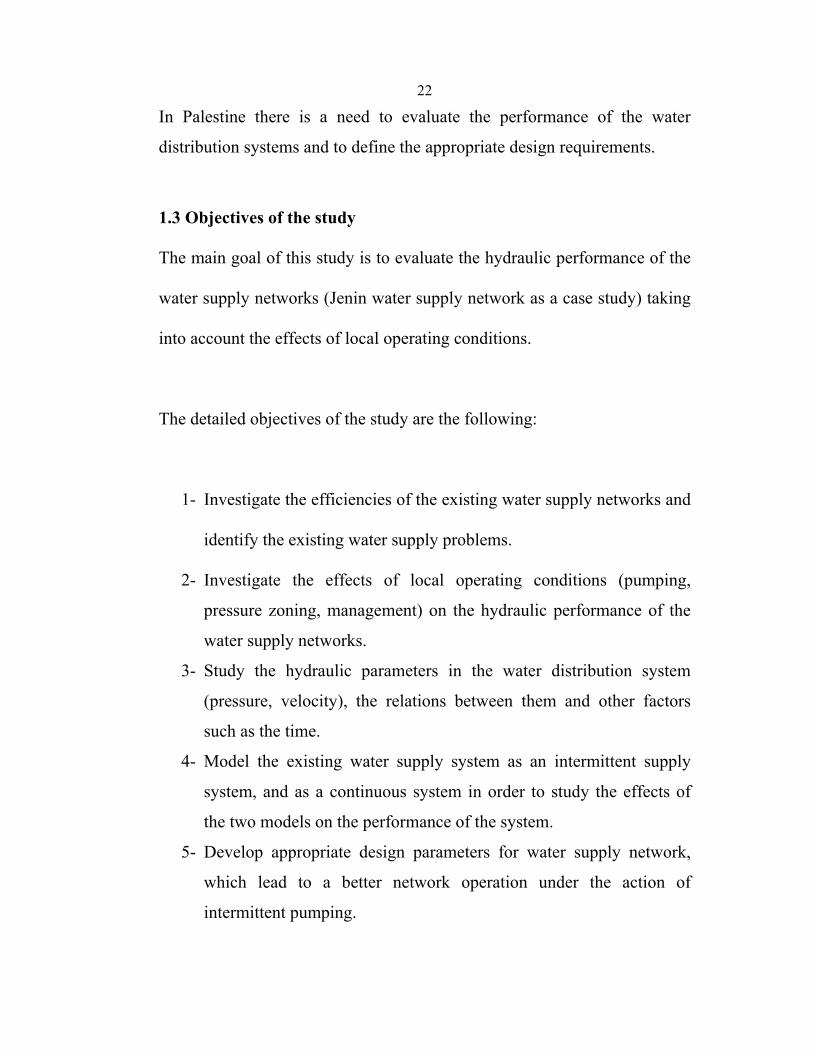
1.3 Objectives of the study
The main goal of this study is to evaluate the hydraulic performance of the
water supply networks (Jenin water supply network as a case study) taking
into account the effects of local operating conditions.
The detailed objectives of the study are the following:
1- Investigate the efficiencies of the existing water supply networks and
identify the existing water supply problems.
2- Investigate the effects of local operating conditions (pumping,
pressure zoning, management) on the hydraulic performance of the
water supply networks.
3- Study the hydraulic parameters in the water distribution system
(pressure, velocity), the relations between them and other factors
such as the time.
4- Model the existing water supply system as an intermittent supply
system, and as a continuous system in order to study the effects of
the two models on the performance of the system.
5- Develop appropriate design parameters for water supply network,
which lead to a better network operation under the action of
intermittent pumping.

23
6- Study the variations of the water level in roof tanks and measured the
water consumption each day for a certain period to derive the daily
peak factors for different consumers.
1.4 Main components of the methodology of the study
1- The Jenin water distribution system and representative sectors in the
network have been investigated as a case study.
2- Detailed information and maps of the Jenin water distribution system
that are necessary to carry out the study have been provided by the
municipality of Jenin, and a letter has been sent to the municipality
of Jenin to explain the goals and the objectives of the study in order
to contribute in the work and to have an approval.
3- Field measurements for the variations of the water levels in number
of roof tanks for different consumers have been measured by
periodic readings and these readings have been analyzed to study the
change in the water level of the storage tanks and the water
consumption in order to develop the daily peak factors for different
consumers and calculate the average peak factor.
4- Field measurements, which have been done in previous studies in a
pilot zone have been studied and investigated to get a better idea
about the distribution system of Jenin city. The results of
measurements carried out in the pilot zone used to determine the
unaccounted for water (UFW) for the whole network and the
consumption figures.
5- The existing water supply network has been modeled using a
computer program (WaterCad) as in reality (intermittent water

24
system) depending on the existing situation of operating the different
parts of the network.
6- The water supply system of Jenin city has been redesigned as a
continuous supply depending on fixed pattern, assuming the
availability of water sources, and the using of pressure-reducing
valves to reduce the high pressures in the system.
1.5 Literature Review
Several researches have been made to study the behavior of water
distribution systems, and to reach an optimal solutions and assumptions in
order to improve the hydraulic performance, cost effective, and to increase
the efficiencies of the water supply networks.
Jarrar H (1998) studied the hydraulic performance of water distribution
systems under the action of cyclic pumping; the results show that the
network under consideration is exposed to relatively high-pressure values
throughout. The velocity of the water through the network attained also
high values. These high values of pressure and velocity have negative
effects on the performance of the network [4].
Masri M (1997) studied the optimum design of water distribution networks.
A computerized technique was developed for the analysis and optimal
design of water distribution networks. The results show that the selection of
the hydraulic restrictions should be reasonable and reflects the real capacity
of the water distribution system [5].

25
Naeeni S (1996) developed a computer program, which enables to obtain
the optimum design of various kinds of water distribution networks so that
all constraints such as pipe diameters, flow, velocities, and nodal pressures
are satisfied [6].
AL-Abbase R (2000) showed that the optimum design of water distribution
systems is a theoretical purpose, and cannot be achieved completely. His
study dealt with evaluation the performance of five big sectors in Mosul
city. A computerized technique was developed to obtain the optimum
design, which achieves the demands of the consumers at lowest cost using
the commercial pipes [7].
James, Liggest and Chen (1994) made a study about distribution systems.
Data about pressure and flow rate were obtained by continuous monitoring
of their system. Transient analysis, time lagged calculations and inverse
calculations were applied as a tool for calibration and leak detection [8].
James E.Funk (1994) studied the behavior of water distribution systems
during transient operations. He concluded that during transient operations,
pressure much higher than steady state values could develop. The causes of
transient operation can be a result of pumps stopping or starting, valves
opening or closing, and system startup or shut down [2].
Genedese,Gallerano and Misiti (1987) were involved in the optimal design
of closed hydraulic networks with pumping stations and different flow rate
conditions. Their study had two aims in the design of water distribution
systems. The first is minimum values of peizometric heads at the nodes.
The second is maximum values of velocities in the branches [9].

26
Perez,Martinez and Vela(1993) suggested a method for optimal design by
considering factors other than pipe size. Pressure reducing valves were
suggested to reduce the pressure in the down stream pipes [10].
Vairavamoorthy, Akinpelu,Lin and Ali (2000) suggested a new method of
design sustainable water distribution systems in developing countries. They
developed a modified mathematical modeling tool specifically developed
for intermittent water distribution systems. This modified tool combined
with optimal design algorithms with the objective of providing an equitable
distribution of water at the least cost forms the basis of this new approach.
They also develop guidelines for the effective monitoring and management
of water quality in intermittent water distribution systems. A modified
network analysis program has been developed that incorporates pressure
dependent outflow functions to model the demand [11].
Battermann A and Macke S (2001) developed a strategy to reduce technical
water losses for intermittent water supply systems in AlKoura District-
Jordan. This work describes the development of a practical simulation
model for the intermittent supply of water. Standard software is used to
implement the model: Arc View GIS and the free hydraulics software
EPANET. The model has been applied to the water supply network of the
village Judayta (AlKoura District) and successfully calibrated with a loggin
campaign [12].
Vairavamoorthy and Lumbrs (1998) studied the leakage reduction in water
distribution systems depending on optimal valve control. The inclusion of
pressure- dependent leakage terms in network analysis allows the
application of formal optimization techniques to identify the most effective

27
means of reducing water losses in distribution systems. They describe the
development of an optimization method to minimize leakage in water
distribution systems through the most effective settings of flow reduction
valves [13].
M.Y.Abdel-Latif (2001) assess the hydraulic behavior and evaluate the
global performance of Bani Suhila City water distribution network by
developing a computer model for a distribution network under actual
existing and alternative conditions, especially involving intermittent
supply. The performance of the network was evaluated from a hydraulic
point view using a systematic, engineering approach, and the results
indicated that the performance was adequate and the system provided an
acceptable level of service based on pressure considerations [14].
Yan J (2001) modeling contaminant intrusion into water distribution
systems. He develops measures to minimize the risk of contamination, and
improve the management of water quality in drinking water distribution
systems. As a result of his research, a contaminant ingress model will be
developed, consisting of three main components: 1. A pipe condition
assessment to evaluate the condition of the pipe. 2. A contaminant seepage
component that simulate contaminant flow. 3. A contaminant ingress
component to predict the pollution prone areas where contaminants may
enter into the pipes of water distribution systems [15].
Saleh A (1999) made a study, considering with the internal evaluation of
Palestinian water industry. His study analyses the performance of
Palestinian water supply companies (WSCs). The study shows that large-
scale Palestinian water supply companies perform much better than small-

28
scale companies. Moreover, the delegated public water supply companies
perform better than the municipal water departments [16].
1.6 Study Structure
This research consists of seven chapters including the introduction.
In chapter two, description of Palestinian water resources and the state of
the existing water distribution systems, also the challenges to be faced the
water sector in the Palestinian territories.
Chapter three, details on the water distribution systems, types of the supply
systems, methods of distribution, components and principles of pipe
network hydraulics in addition to the main hydraulic design parameters
were investigated and studied.
Chapter four contains details on the concept of intermittent water supply
systems, the problems of the intermittent systems, comparison between the
continuous supply and the intermittent systems, and the proposed methods
of modeling the intermittent water supply systems.
Chapter five describes the state of the jenin water distribution network,
theoretical background, existing situation, storage facilities, pipes and
materials, valves and regulating devices, tertiary network and ways of
delivery to customers.
Chapter six, modeling the jenin water distribution network as an
intermittent supply system and continuous supply system, studying a pilot
zone in the network to develop the water consumption and unaccounted for

29
water (UFW), studying the variations in levels of roof tanks to derive the
peak factors, and analyze the outputs of these works, study the effects of air
release valves at customer meters, and evaluation the effects of water
hammer phenomena in the system.
In chapter seven, results, and logical conclusions of modeling the network
as intermittent and continuous supply system that will lead to a better
network performance are stated.

30
Chapter Two
Palestinian Water Resources
2.1 Introduction
Present water supplies in the palestinian regions are neither adequate to
provide acceptable standards of living for the palestinian people, nor
sufficient to facilitate economic development as a result of the limitation on
supply and restrictions on developing new water resources and supply
infrastructure.
Current average daily consumption rate in the West Bank for the 86%
population that is served from the piped system is only about 50
liters/person, while in Gaza Strip, despite the fact that 98% of the
population have access to a piped water supply with an average per capita
consumption of 80 l/c/d, considering the quality of water is only 14% of the
recommended world health organization (WHO) minimum.
The limited water resources in the Palestinian governorates face the
challenge not only to supply the various water sectors with their water
demand, but also has to secure water to meet the increasing needs for
people in the future.
The present situation in the water sector on Palestine and the challenges to
be faced are summarized below:
- Water resources in the region are extremely scarce and disputable.

31
- Water demand is continuously growing.
- Water supply and sanitation services are inefficiently delivered and
inadequate.
- Tariffs are generally inadequate.
- Consumption and water losses are excessive.
- Insufficient water harvest activities.
- Wastewater is unavailable, inadequate or not well functioning.
The Israeli occupation of Palestinian land had adverse impacts in many
respects. In the water sector, these have included the illegal control, by
Israeli military order, of all water resources in Palestine, including the
licensing, operation, and administration of wells, prohibition of new well
drilling without authorization, over extraction from and degradation of
aquifers, inequitable allocation of water between Israeli settlements and
Palestinian municipalities [18].
The one fact that is indisputable, however, is that the Palestinians have no
decision making power in their own water future [19].
2.2 Main Water Resources in Palestine
The water resources of Palestine include:
1.Ground water: is the main source of water in Palestine.
- West Bank Mountain Aquifer: is the main source of water. It is mainly
composed of Karstic Limestone and Dolomite formations of the
Cenomanian and Turonian ages and is mostly recharged from rainfall on
the west bank mountains of heights greater than 500 meters above mean

32
sea level. The annual renewable freshwater of this aquifer ranges from
600 MCM to 650 MCM [18].
The west bank aquifer system has three major drainage basins:
1- The western basin, supplied and recharged from the West Bank
mountains, located within the boundaries of the West Bank and 1948
occupied territories [20].
2- The northeastern basin, which is located inside the West Bank near
Nablus and Jenin and drains into the Eocene and Cenomanian –
Turonian aquifer under the north of the west bank [20].
3- The eastern basin, which is located within the West Bank and the
springs from which represent %90 of spring discharge in this area [20].
West Bank Palestinians exploit currently a mere 115 MCM – 123 MCM,
The other amount is exploited by the Israelis [20]. The existing situation
and the present water crisis is not chiefly one of insufficient supply, but of
unquotable and uneven distribution.
- Gaza Coastal Aquifer: it is part of the coastal aquifer, has been
continuously over-pumped for quite some time in large part to serve the
high population. Its annual safe yield is 60 MCM - 65 MCM [21].
The water table has been pumped to far below the recharge rate, and there
is evidence of deteriorated water quality of the aquifer [20].
The main Gaza Aquifer is a continuation of the shallow sandy/sandstone
coastal aquifer, which is of the pliocene-pleistocene geological age. About

33
2200 wells tap this aquifer with depths mostly ranging between 25 and 30
meters [21].
Table (2.1)
*Ground water resources in Palestine (in MCM /year) ــــــــــــــــــــــــــــــــــــــــــــــــــــــــــــــــــــــــــــــــــــــــــــــــــــــــــــــــــــــــــــــــــــــــــــــــــــــــــــــــــــــــــــــــــــــــــــــــــــــــــــــــــــــ
Basin Israeli Palestinian Palestinian Quantities Total estimated
consumption consumption consumption available for yields of aquifers
from wells from springs development
ـــــــــــــــــــــــــــــــــــــــــــــــــــــــــــــــــــــــــــــــــــــــــــــــــــــــــــــــــــــــــــــــــــــــــــــــــــــــــــــــــــــــــــــــــــــــــــــــــــــــــــــ
Western 340 20 2 362
Northeastern 103 25 17 145
Eastern 40 24 30 78 172
Gaza aquifer 55
Total 483 69 49 78 734
ــــــــــــــــــــــــــــــــــــــــــــــــــــــــــــــــــــــــــــــــــــــــــــــــــــــــــــــــــــــــــــــــــــــــــــــــــــــــــــــــــــــــــــــــــــــــــــــــــــــــــــــــــــــ
*Data taken from Article 40 of Oslo B Agreement [24] .
2.Jordan River
It is the only river, which the west bank has access to. The west bank uses
nothing of its water. The average annual flow of this river is about 1200
MCM [22]. The riparian of the Jordan River are Lebanon, Syria, Palestine
and Jordan. Only three percent of the Jordan River’s basin falls within the
land pre 1967 boundaries.
3.Springs
There are 297 springs in the West Bank, 114 out of which are considered to
be the main ones with substantial yield quantities. Usually there are
fluctuations in the yield of some of these springs in the different years,

34
depending on the rainfall quantities, and thus the recharge to ground water.
However, their average annual yield is estimated to be around 60.8 MCM
/year [23].
4.Non-conventional water resources-Cisterns
Cisterns are of major importance in the west bank governorates. The water
quantities in the cisterns are used mainly for domestic purposes. The
typical form of these cisterns is to collect water from the roofs of the
buildings in the winter season and store it in an underground hole in most
of the cases [20].
Cisterns act as a major source of domestic water supply in the localities that
do not have water supply networks. It is estimated that 6.6 MCM is utilized
from the cisterns. In localities where water networks exist, cisterns still act
as another “good” source of domestic water supply [25].

35
Map (2.1)
Water resources in Palestine

36
2.3 Water supply
Around 88% residing in 345 localities in the West Bank have piped water
supply systems, while 12% of inhabitants residing in 282 localities do not
have the service. In terms of localities (i.e., towns and villages), 55% of the
localities in the west bank have piped water supply systems and 45% are
without this service [20].
2.4 Water Demand
The indicator for measuring the level of water consumption is the amount
of water consumed per capita per day (l/c/d). Water consumption is a
function of availability, religion, climate conditions, and affordability.
Another indicator used in measuring the level of water consumption is the
quality of delivered water. In general, water utilities have to follow WHO
standards for domestic water [16].
The total water use by municipal and industrial sectors in Palestine during
the year 1999 was estimated to be 101 MCM. An amount of 52 MCM was
used in the West Bank , whereas a total of approximately 49 MCM was
used in the Gaza Strip . The water consumed by the agricultural sector is
estimated to be 172 MCM [26].
2.5 Future potential water demand
A demand of 432 MCM is projected for the year 2020. This estimation is
based on WHO minimum and average domestic water consumption

37
standards of 100 l/c/d and 150 l/c/d [20]. The estimated agriculture water
demand by the year 2020 is about 353 MCM [26].
If the projections of Palestinian demand are based on equal municipal and
industrial Israeli per capita water consumption, then the total municipal and
industrial Palestinian water demand will be 852 MCM for the year 2020
[27].
The Palestinian water sector should achieve an amount of around 785
MCM/year by the year 2020. This amount is about three times the available
supply at present, but at the same time not higher than the Palestinian water
rights from the renewable water resources [20].
2.6 Palestinian water supply industry indicators
Eight performance indicators were distinguished as water severs indicators,
for the Palestinian water supply industry. There are [16]:
1. Low service timing: 3 – 7 days per week
2. Very low water consumption: 35 – 120 l/c/d
3. High level of UFW: 22.3% - 50.4%
4. Wide range of the level of productivity: 6.5 – 12.9 staff/1000 connection
5. Very wide range of an average tariff: 0.19 – 1.69 $/ m3
6. Very wide range of price of new connections: 86 – 627 $/connection
7. Low figures of cost recovery: 62% - 188%
8. Reasonable bill collection efficiency: 80% - 175%
The strategies proposed to overcome the problem of water crisis can be
summarized as following:

38
- The Palestinian water rights should be secured.
- To make the water institutions are able to govern and manage water
effectively it should be strengthen.
- Implement a combination of water supply and demand measures.
- Agriculture sector should be reform and modernize.
- Protect water quality and enhance the sanitation sector.
- Generate knowledge and help in the uptake of existing knowledge in
relation to water use efficiency and water quality [20].

39
Chapter Three
Water Supply Systems
3.1 Introduction
The objective of water distribution systems is to deliver water of suitable
quality to individual users in an adequate amount and at a satisfactory
pressure. It should be capable of delivering the maximum instantaneous
design flow at a satisfactory pressure.
The water distribution networks should meet demands for potable water. If
designed correctly, the network of interconnected pipes, storage tanks,
pumps, and regulating valves provides adequate pressures, adequate
supply, and good water quality throughout the system. If incorrectly
designed, some areas may have low pressures, poor fire protection, and
even health risks [32].
The water distribution networks, which is typically the most expensive
component of a water supply system, is continuously subject to
environmental and operational stresses which lead to its deterioration.
Increased operation and maintenance costs, water losses, reduction in the
quality of service and reduction in the quality of water are typical outcomes
of this deterioration [33].

40
3.2 Types of Water Distribution Systems
3.2.1 Branching Systems
This type of distribution networks is the most economical system, and
common in the developing countries due to its low cost. In this system,
when there is need for developing the network, new branches follow that
development and new dead ends will be constructed.
The branching systems have some disadvantages such as the following:
- The dead ends cause accumulation of sediments, which result in
increasing contamination and health risks.
- The maintenance operation upstream of the network will prevent
water to reach the down stream due to the interruption of the whole
area of maintenance.
- The fluctuating demand causes high-pressure oscillations.
3.2.2 Grid Systems
There are no dead ends in this type of distribution networks. The
maintenance operation did not effect the interruption on the whole area as
in the branching system, this type of layout is highly desirable because, for
any given area on the grid, water can be supplied from more than one
direction. This results in substantially lower head losses than would
otherwise occur and, with valves located properly, allows for minimum

41
inconvenience when repairs or maintenance activities are required. The
whole area is covered with mains that form the grid system.
3.2.3 Ring Systems
The mains form a ring around the area under service, secondary pipes
connecting the mains and delivering the water to the consumers.
3.2.4 Radial Systems
The area under service in the radial system is divided into subareas , and a
storage tank is placed in the center of each subarea to supply water to the
consumer.
The following figure shows the types of the water distribution systems
Figure (3.1)
Types of the water distribution systems
Branch System Grid System Circular System Radial System

42
3.3 Methods of Water Distribution
3.3.1 Gravity Distribution
This is possible , when the source of supply water is at some elevation
above the city , so that sufficient pressure can be maintained in the mains
for domestic and fire services . The advantage of this method of
distribution is saving power that needed for pumping.
3.3.2 Distribution by Pumping Without Storage
In this method of distribution, water is pumped directly into the mains with
no other outlet than the water actually consumed.
The pumping rate should be sufficient to satisfy the demand. This method
is the least desirable way of distribution; the power failure leads to
complete interruption in water supply.
An advantage of direct pumping is that a large fire service pump may be
used which can run up the pressure to any desired amount permitted by the
construction of mains [28].
3.3.3 Distribution by means of pumps with storage
In this method an elevated tanks or reservoirs are used to maintain the
excess water pumped during periods of low consumption, and these stored
quantities of water may be used during the periods of high consumption.

43
This method allows fairly uniform rates of pumping and hence is
economical [28].
3.4 Principles of Pipe Network Hydraulics
Flow in a pipe network satisfies two basic principles, conservation of mass,
and conservation of energy.
3.4.1 Conservation of Mass- Flows Demands
Conservation of mass states that, for a steady state system, the flow into
and out of the system must be the same [29]. This principle is a simple one,
at any node in the system under incompressible flow conditions; the total
volumetric or mass flow in must equal the mass flow out (less the change
in storage).
This relationship holds for the entire network and for individual nodes.
One mass balance equation is written for each node in the network as:
∑ Q in - ∑ Q out = Q demand (3.1)
Where: ∑ Q in : flows in pipes entering the node.
∑ Q out : flows in pipes exiting the node.
Q demand : the user demand at that location.

44
Separating the total volumetric flow into flows from connecting pipes,
demands, and storage, we obtain the following equation [32]:
∑ Q in ∆t = ∑ Q out ∆t + ∆VS (3.2)
Where : ∑ Q in : the total flow into the node.
∑ Q out : the total demand at the node.
∆VS : is the change in the storage.
∆t : is the change in time.
The continuity equation at node j can be expressed as following :
i=NP( j )
∑ Qij - Cj = 0 (3.3) i=1
Where: ∑ Qij : is the algebraic sum of the flow rates in the pipes
meeting at the node j .
Cj : is the external flow rate at node j.
NP( j ) : is the number of pipes meeting at junction j.

45
3.4.2 Conservation of Energy
It is the second governing equation that describes the relationship between
the energy loss and pipe flow. The head losses through the system must
balance at each point. For pressure networks, this means that the total head
loss between any two nodes in the system must be the same regardless of
what path is taken between two points.
The head loss must be sign consistent with the assumed flow direction
(gain head when proceeding opposite the direction of flow, and lose head
when proceeding with the flow) [32].
As shown in the figure (3.2) below, the combined head loss around a loop
must equal zero in order to achieve the same hydraulic grade that was
started with.
Loop from A to A:
0 = HL1 + HL2 - HL3 (3.4)
Figure (3.2)
Conservation of Energy
A HL3 C
HL1 HL2
B
46
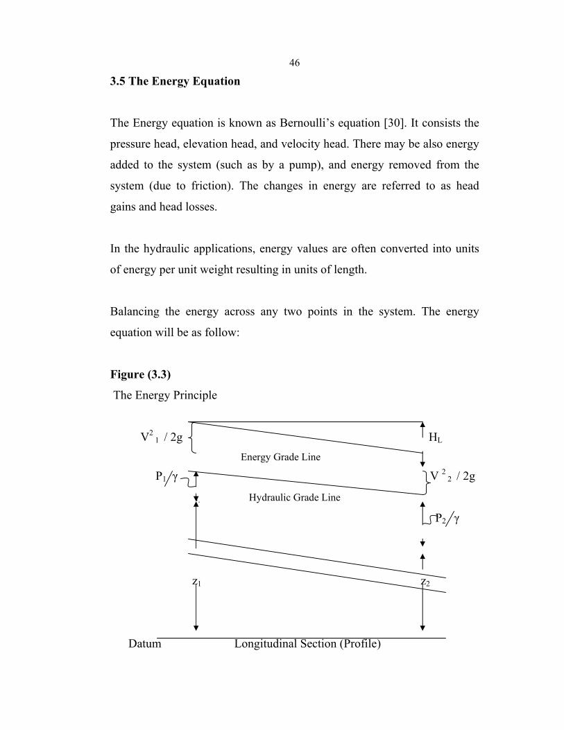
3.5 The Energy Equation
The Energy equation is known as Bernoulli’s equation [30]. It consists the
pressure head, elevation head, and velocity head. There may be also energy
added to the system (such as by a pump), and energy removed from the
system (due to friction). The changes in energy are referred to as head
gains and head losses.
In the hydraulic applications, energy values are often converted into units
of energy per unit weight resulting in units of length.
Balancing the energy across any two points in the system. The energy
equation will be as follow:
Figure (3.3)
The Energy Principle
V2 1 / 2g HL
Energy Grade Line
P1 γ V 2 2 / 2g
.. Hydraulic Grade Line
P2 γ
z1 z2
Datum Longitudinal Section (Profile)

47
P1 / γ + z1 + V2 1 / 2g + HG = P2 / γ + z2 + V 2
2 / 2g + HL (3.5)
Where : P : is the pressure (Ib/ft2 or N/m2 )
γ : is the specific weight of the fluid (Ib/ft3 or N/m3 )
z : is the elevation at the centroid ( ft or m )
V : is the fluid velocity ( ft/s or m/ s )
g : is gravitational acceleration ( ft/s2 or m/ s2 )
HG : is the head gain, such as from a pump (ft or m )
HL : is the combined head loss (ft or m )
3.6 Energy Losses
There is a combination of several factors that cause the energy losses. The
main reason of the energy loss is due to internal friction between fluid
particles traveling at different velocities. The movement of any fluid
through a conduit results in a resistance to flow and this resistance or
energy loss is referred to as friction .

48
The other reason causes energy loss is due to localized areas of increased
turbulence and disruption of the stream lines such as disruptions from
valves and other fittings in a pressure pipe [32].
The rate of losing energy a long a given length is called friction slope .It is
usually presented as a unit less value, or in units of length per length ( ft/ft ,
m/m , etc.)
3.6.1 Friction Losses
Hazen-Williams equation and the Darcy-Weisbach equation are the most
commonly methods used for determining head losses in pressure piping
systems.
The assumptions for a pressure pipe system can be described as the
following:
- Pressure piping is almost always circular, so the area of flow, wetted
perimeter, and the hydraulic radius can all be directly related to
diameter.
- Through a given length of a pipe in a pressure piping system, flow is
full, so the friction slope is constant for a certain flowrate. This means
that the energy grade and hydraulic grade drop linearly in the direction
of flow.

49
- The velocity must be constant, since the flowrate and cross-area are
constant. This means that the hydraulic grade line (the sum of the
pressure head (P/γ), and the elevation head (z)), and the energy grade
line (the sum of the hydraulic grade line and the velocity head (v2 / 2g)).
Equations that represent the friction losses associated with the flow of a
liquid through a given section can all be described by the following general
equation:
V= KCRXSY (3.6)
Where: V: mean velocity.
C : flow resistance factor
R : hydraulic radius (A/Pw)
RCircular : π.D2 / 4 = D
π .D 4
Pw : wetted perimeter (ft or m) A: cross sectional area (ft2 or m2 ) D : pipe diameter ( ft or m ) S : friction slope x , y : exponents k : factor to account for empirical constant , unit conversion, etc.
50
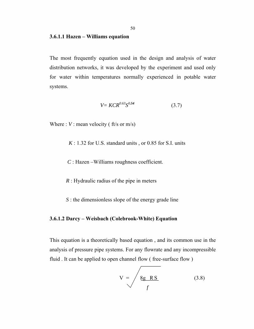
3.6.1.1 Hazen – Williams equation
The most frequently equation used in the design and analysis of water
distribution networks, it was developed by the experiment and used only
for water within temperatures normally experienced in potable water
systems.
V= KCR0.63S0.54 (3.7)
Where : V : mean velocity ( ft/s or m/s)
K : 1.32 for U.S. standard units , or 0.85 for S.I. units
C : Hazen –Williams roughness coefficient.
R : Hydraulic radius of the pipe in meters
S : the dimensionless slope of the energy grade line
3.6.1.2 Darcy – Weisbach (Colebrook-White) Equation
This equation is a theoretically based equation , and its common use in the
analysis of pressure pipe systems. For any flowrate and any incompressible
fluid . It can be applied to open channel flow ( free-surface flow )
V = 8g R S (3.8)
f

51
Where : V : flow velocity (ft/s or m/s )
g : gravitational acceleration (ft/s2 or m/ s2 )
R : hydraulic radius ( ft or m )
f : Darcy-Weisbach friction factor
S : Friction slope
The Darcy – Weisbach friction factor, f, can be found using the Colebrook
equation as follows:
1 K 2.51 (3.9)
=-2 log +
f 14.8 R Re f
Where : K : roughness height ( ft or m )
Re : Reynolds number
3.6.1.3 Reynolds Number
It is an index used to classify flow as either laminar flow (it is a flow
characterized by smooth flow lines) or turbulent flow (it is a flow
characterized by the formation of eddies within the flow)

52
Re = 4 V R (3.10)
ν Where: Re : Reynolds number.
V : Mean velocity ( ft/s or m/s)
R : Hydraulic radius ( ft or m )
ν : Kinematics viscosity ( ft2 / s or m2 /s )
If the number below 2000, flow is laminar. The number is above 4000 the
flow is turbulent. Between 2000 and 4000, may be either turbulent or
laminar flow.
3.6.2 Minor Losses
Minor losses are a result of localized areas of increased turbulence and are
frictional head losses, which cause energy losses within a pipe. A drop in
the energy and hydraulic grades caused by valves, meters, and fittings, the
value of these minor losses is often negligible relative to friction and for
long pipes, and they are often ignored during analysis.
Minor head losses (also referred to as local losses) can be associated with
the added turbulence that occurs at bends, junctions, meters, and valves.
The importance of such losses will depend on the layout of the pipe
network and the degree of accuracy required.

53
The resulting head loss is computed from the following equation:
Hm = K V2 (3.11)
2g
Where : Hm : minor loss ( ft or m )
K : minor loss coefficient for the specific fitting .
V : velocity ( ft/s or m/s)
g : is gravitational acceleration (ft/s2 or m/s2 )
3.6.3 Water Hammer
When the velocity of flow in a pipe changes suddenly , surge pressures are
generated as some , or all , of the kinetic energy of the fluid is converted to
potential energy and stored temporarily via elastic deformation of the
system. As the system rebounds and the fluid returns to its original
pressure, the stored potential energy is converted to kinetic energy and a
surge pressure wave moves through the system. Ultimately , the exess
energy associated with the wave is dissipated through frictional losses .
This phenomenon , generally known as “water hammer” , occurs most
commonly when valves are opened or closed suddenly , or when pumps are
started or stopped . The excess pressures associated with water hammer can
be significant under some circumstances.

54
The maximum pressure surge caused by abruptly stopping the flow in a
single pipe is given by :
a = 4660 (3.12)
[ 1 + Kd/Et ]0.5
Where: k : bulk modulus of the fluid, pounds per square inch
d : internal diameter of the pipe , inches
E : modulus of elasticity of the pipe materials, pounds per square
inch.
t : thickness of the pipe wall, inches
The magnitude of the maximum potential water hammer pressure surge as
illustrated by the above equation is a function of fluid velocity, and the pipe
material . In water distribution systems , water hammer is usually not a
problem because flow velocities are typically low , when higher than
normal flow velocities are expected , consideration should be given to the
use of slow-operating control valves, safety valves , surge tanks, air
chambers, and special pump control systems.
3.7 Hydraulic Design Parameters
The main hydraulic parameters in water distribution networks are the
pressure and the flowrate , other relevant design factors are the pipe
diameters , velocities , and the hydraulic gradients [5].

55
3.7.1 Pressure
The pressure at nodes depends on the adopted minimum and maximum
pressures within the network, topographic circumstances , and the size of
the network [5].
The minimum pressure should be maintained to avoid water column
separation and to ensure that consumers demands are provided at all times.
The maximum pressure constraints results from service performance
requirements such fire needs or the pressure –bearing capacity of the pipes ,
also limit the leakage in the distribution system , especially that there is a
direct relationship between the high pressure and the increasing of leakage
value in the system.
3.7.2 Flowrate
It is the quantity of water passes within a certain time through a certain
section.
Velocity is directly proportional to the flowrate . for a known pipe diameter
and a known velocity , the flowrate through a section can be estimated.
Low velocities affect the proper supply and will be undesirable for hygienic
reasons ( sediment formation may cause due to the long time of retention).
The effect of the velocity on the diameters of pipe system can be observed
from the following equation :

56
V = 4Q (3.13)
π.D2
D = 4Q (3.14)
π .V
Where : D : diameter of the pipe (m)
Q : discharge ( m3 /sec)
V : velocity (m/sec)
From the above equation it is clear that the velocity increasing should
decrease the diameter value.

57
Chapter Four
Intermittent water supply systems
4.1 Introduction
The available water sources through the world are becoming depleted and
this has brought into focus the urgent need for planned action to manage
water resources effectively for sustainable development.
The problem of water scarcity in urban areas of developing countries is of
particular concern and as the water quantity available for supply generally
is not sufficient to meet the demands of the population, water conservation
measures are employed [11].
Providing a water supply for a community involves tapping the most
suitable source of water, ensuring that it is safe for domestic consumption
and then supplying it in adequate quantities.
The world health organization defines [36]. :
Safe water as; water that does not contain harmful chemical substances or
micro-organisms in concentrations that cause illness in any form, and
adequate water supply as; one that provides safe water in quantities
sufficient for drinking, and for culinary, domestic and other household
purposes so as to make possible the personal hygiene of members of the

58
household. A sufficient quantity should be available on a reliable, year-
round basis near to, or within the household where the water is to be used.
One of the most common methods of controlling water demand is the use
of intermittent water supplies, usually by necessity rather than design. It
has been widely reported in the literature that the majority of water supply
systems in developing countries are intermittent.
It is of interest to note that 91% of systems in South East Asia are
intermittent as reported by WHO survey [31]. Practically all-Indian cities
are reported to operate intermittent systems [34].
The design of water distribution systems in general has been based on the
assumption of continuous supply. In most developing countries water
supply is not continuous but intermittent, and this could have been foreseen
at the design stage. This has resulted in severe supply, pressure problems in
the network and great inequities in the distribution of water.
Most design engineers in the developing world are aware that their
approach to design is incorrect, but argue there is no alternative since there
are no proper design tools developed specifically for intermittent systems
[11].
It is evident from literature surveyed that the design of distribution
networks operating intermittent supplies has in general been based on the
assumption of continuous supply, the concepts and methods used are
identical with those used in the developed countries [35].

59
4.2 Intermittent supply
An important component of a water supply system is the distribution
network, which conveys water to the consumer from the sources. These
systems constitute a substantial proportion of the cost of a water supply
system, in some cases as much as half the overall cost of the system [35].
The design of supply systems in most of the developing regions based on
the assumption of direct supply, although most of these systems are
intermittent systems, which result in severe supply, pressure losses and
great inequities in the distribution of water.
The problems of the intermittent supply systems:
- Overall shortage of water.
- Insufficient pressure in the distribution system (several areas in the
network had zero pressure)
- Inequitable distribution of the available water.
- Very short duration of supply.
A serious problem arising from intermittent supplies, which is generally
ignored, is the associated high levels of contamination. This occurs in
networks where there are prolonged periods of interruption of supply due to
negligible or zero pressures in the system. The factor that is most related to
contamination is duration of supply [35].

60
Both continuous and intermittent water distribution systems might suffer
from the contaminant intrusion problem, and the intermittent systems were
found more vulnerable of contaminant intrusion [15].
As reported by several studies, the disadvantages of the intermittent supply
systems can be summarized as follows:
- Systems do not operate as designed.
- Reservoir capacities are underutilized.
- There is frequent wear and tear on valves.
- More manpower is needed.
- Contaminated water requires consumer treatment.
- High doses of chlorine are needed.
- Over sizing the network is needed to supply the necessary quantities
in a shorter time.
- Consumers have to pay for storage and pumping.
- Water meters malfunction, which can lead to a loss of revenue and
customer disputes.
- In case of fire, immediate supply is unavailable.
4.3 Modeling of direct (continuous) supply systems and intermittent
supply systems
4.3.1 Modeling of Direct (continuous) supply systems
In the continuous supply systems, water is conveyed through the
distribution network continuously without interruptions. The consumers

61
use water at any time without any need for individual roof and or ground
storage tanks [3].
The main factors required to achieve direct water supply are summarized as
follows:
- Enough water at source: to meet consumer’s requirements for water
(the demand increases due to availability of water)
- A good and reliable distribution network: to guarantee enough water
with acceptable pressure to all consumers.
- Effective system parameters: capable pump stations, and suitable pie
diameters.
- Successful monitoring policy: to discover any interruptions, and to
detect damaged pipes early as possible, to reduce leakage.
Operating of system components, pumps and reservoirs, in the continuous
supply systems is a result of consumers needs: with reduced demand in the
night periods, pumps may operate at lower level and balancing reservoirs
may be refilled, whereas during the maximum demand periods, the pumps
will operate at their maximum capacity and the reservoirs will supply parts
of the distribution network.
The water distribution network in the continuous supply systems should be
designed to wish stand the range of pressures corresponding to the
minimum and maximum supply conditions.
In the continuous supply systems, the hydraulic relation between the
demand and supply water is clear. The demand in the nodes or nodal water

62
demand is the water consumption multiplied by the number of residents
living around. The average demand will be subjected to hourly variations,
which mean the demand pattern based on the differences in living
standards, industrial water use, etc.
4.3.2 Modeling of Intermittent supply systems
The regime of intermittent water supply, is applied as mentioned in the
developing areas, due to the scarcity of drinking water, and deteriorated
distribution networks.
In the intermittent supply systems, the consumers depend on the individual
roof and /or ground storage tanks to provide their daily needs of water for
domestic, industrial, and other uses. This means that in the periods of use,
the consumption of water is not necessarily provided from the network
directly, but may be from the roof tanks and /or ground storage tanks in
which water was stored when the pressure head in the system was higher
than the reservoir. In this case the consumers of water are not restricted
only by the pressure that is available in the distribution network, but also
they are restricted by the capacity of the roof tanks and ground storage
tanks.
From the hydraulic point view, when the consumers are using the water
from their roof tanks, they are disconnected from the distribution system,
and two independent patterns can be distinguished in this case: the first
pattern at the consumer’s tap which is actually a consumption pattern and
may be equal for all domestic consumers, and the second pattern is at the

63
tank which is actually a filling pattern, and it is a consequence of the
hydraulic operation of the network, representing a pressure related
discharge , and its different for each node in the network.
The consumers faraway from the source of water supply in the intermittent
systems will need to be more patient, especially that the refilling of their
roof tanks will start later and go slower than for those consumers closer to
the water source.
Intermittent supply yields afundamentaly different demand pattern than
continuous supply, in fact there is no demand pattern: the storage tanks of
the customers will fill up whenever the systems provides water, until they
are full and the float valve closes [12].
4.4 Proposed methods for modeling inermittent water supply systems
The overall shortage in water availability in the most developing countries
necessitates intermittent supply at a low per capita supply rate. These
conditions force consumers to collect water in storage tanks.
Storage is an important feature of such systems since it is the storage
facilities that provide water during non-supply hours. Because of the low
supply rate of water and the intermittent nature of supply, the demand for
water at the nodes in the network are not based on notions of diurnal
variations of demand related to the consumers behavior (as with networks
in developed countries), but on the maximum quantity of water that can be
collected during supply hours [35].

64
4.4.1 Modified analysis tools
A modified network analysis program has been developed by the water
development research unit at south bank university (London) that
incorporates pressure dependent outflow functions (PDO) to model the
demand. This model consists of four main components. This approach is
far more sophisticated and may provide superior results, and it requires
more specialized software:
1. Demand model
This model forecasts the end-users demand profile (intensity and
distribution of usage over a given period of supply). Data needed for this
model includes: type of connection, time of supply, duration of supply, and
pressure regime [35].
2.Secondary network model
In this model, the primary node assumed to be a constant head, and this
node providing water to the secondary network. Such methods have been
developed and take into account the hydraulic behavior of the secondary
network [37].
3.Network charging model
This model predicts the time at which different users receive water and
simulates the charging up of the network after supply resumes [35].
4.Modified network analysis method (pressurized flow)

65
This model has been developed to model the demand or outflow. The
network governing equations are solved using the gradient algorithm of
Todini and Pilati (1987) [38].
4.4.2 Modeling of nodal demand as pressure related demand
The relation between pressure and demand can be illustrated obviously by
the relation between leakage losses in the water distribution networks and
the pressure. At low peaks through night hours the pressure in the system
will be high and the leakage losses are expected to increase. At high peaks,
the pressure will be small and the leakage losses are expected to decrease.
When the pressure in the system is higher than the elevation of the tank, the
filling will start. It is clear that, the higher the pressure is, more water will
enter into the tank, following the Bernoulli equation.
Figure (4.1)
Illustration of Reservoir Operation

66
The filling of the roof tanks is output of pressure related demand, so it
could be justified to model them as pressure related demand, but the results
will not take into account the level variation in the tank, this lead to the
conclusion that the tank not necessarily be empty, when the pressure in the
nodes is not sufficient.
4.4.3 Modeling as equivalent reservoir
The principle of this approach is representing each cluster of roof tanks in
the distribution system by one large but shallow reservoir. The assumed
reservoir should have a large surface area with volume equal to the total
volume of roof tanks and a depth of 1 m (as in reality), and this reservoir
should be given an elevation equals to the house height [3].
This way of modeling represents the water level variations in the roof tanks
in the case of using special software which taking into account the demand
in the tanks. It can be also used in the process of modeling nodal demand as
pressure related demand.
In this model, the demand in the actual nodes modeled as zero, and the
water consumption is specified at the reservoirs. The water utilization is
based on the availability of water in the individual storage tanks or
proposed reservoirs.

67
Chapter Five
State of the Jenin Water Distribution Network
5.1 Theoretical Background
5.1.1 Geographical, Topographical and Geological Situation
The Jenin city is located in the northern part of Palestine, it is bounded by
the Nablus and Tulkarm districts from the south and southwest, and by the
1948 cease- fire line from the other directions, lying in the southern corner
of the Marj – Ibn – Amer plain. It is consider one of the best agricultural
areas in Palestine [39].
Topographically, the Jenin district is located between 90 and 750 m above
sea level [39]. The altitude levels of Jenin city range from 100 to 280 meter
above sea level, the legal boundaries of the city have been extended, to now
cover 18.2 km2 [40].
The soil conditions in Jenin are dominated by sand and clay for the lower
areas, mainly along Wadi Jenin (Nablus road) up to the Sabah al Khair
region in the north; the slopes of the two hills Al Gaberiat and Al Marah
are dominated by rock [40].

68
Map (5.1)
Map of Palestine showing the location of Jenin City

69
5.1.2 Hydro-geological, climate, Temperature, and Rainwater patterns
Ground water resources in the Jenin area are derived from the northeastern
and western aquifer system. There are two aquifer systems utilized in the
Jenin district, the two exposed aquifer systems are, Upper cenomanian –
turonian aquifer system, which is composed of carbonate rocks “dolomite
and limestone” with thickness ranging from 185 m to 475 m, and the
Eocene aquifer system, this aquifer system overlies the upper cenomanian –
turonian aquifer system, with a transition zone of chalk of variable
thickness ranging from 0 to 480 m is in between, in this system, lime stone
rocks form an aquifer while chalk rock form an aquiclude [41].
The static water level in the Jenin district shows that they directly recharge
from rainfall, and yields from Eocene wells are highly dependent on
seasonal rainfall, ranging from zero to 100 m3/h. The water levels in the
Jenin area can be found at 50 m below ground level, unless they appear on
the surface in the form of springs, either at the interface of chalks, or as a
result of faults [40].
The climate of the Jenin area is governed by its position on the eastern
Mediterranean; the summer season in the Jenin area is dry and hot, while
the winter is moderate and rainy. The average maximum temperature from
June to August is 33.6 c, and the average minimum is 19.3 c [39].
The mean annual rainfall in the Jenin area is 528 mm; the rainy season in
the Jenin district starts in the middle of October and continues to the end of
April. Approximately 3.2% of the annual rainfalls in October, while almost

70
80% falls during November through February. In March, precipitation
usually decreases to 12% of the rainfall [39].
Snowfall is rare in the Jenin district. From 1983 to 1996, snowfall was
recorded only in January and February 1992, which as considered an
exceptionally cold and wet year [40].
5.1.3 Industrial and economic development
The dominant economic activity in the Jenin district is agriculture,
particularly in the historically fertile Marj-Ibn-Amer and the plains around
Jenin city where irrigated agriculture predominates.
Recently, industry has started to play an important role as a source of
income in this district, plastic, fodder, food and beverages, paper and
cartons in addition to concrete block and stone-cutting factories and
workshops, have been established.
Jenin town presently has no major industry, besides small scale enterprises
and the busy market, the future development will be directly connected to
the political situation, currently there are preparations to set up a huge
industrial zone in the north of Jenin town close to the borders, this project
will certainly have a major influence on the development of the town, but
its influence cannot be estimated at the moment.

71
5.1.4 Population Projection
The figures regarding the population of Jenin vary from source to source,
these differences not only for the present population, according to sources
of Jenin municipality, PCBS, PECDAR, PWA, MOPIC, but also the
growth factors for the years to come.
The figure for the present population of Jenin was set as being 41300,this
estimating is an interpolation between the present population according to
PCBS statistics (38400) [42], and the figures derived from the number of
house connections multiplied with the average house hold size (44200)
[40].
The average population growth considered being (4.08% for 1999 and
changing to 2.31% up to the year of 2024, according to PCBS figures [42].
5.1.5 The Structure of The Town
Jenin city is one of the main urban centers in the north of the West Bank,
maintenance and expansion of infrastructure was almost not existent during
the years of occupation. The existing infrastructure lacks integrated
planning, in poor conditions, short of capacity and generally cannot meet
present standards of basic infrastructure requirements [40]. The existing
division of the Jenin town consists of 31 wards.
5.1.6 OSLO – II- Convention limitations
With the Madrid conference in October 1991, the Oslo II interim
agreement was signed in 1995 between the Palestinian authorities and the

72
occupations authorities, according to this convention, the utilization of
water resources in the West Bank is regulated. This convention is an
interim agreement only and might be subject to changes in the future.
In article 40 of the interim agreement (1995), it was agreed that the
Palestinian would be allowed to use 196 MCM/year as shown in the
following table:
Table (5.1)
* Israeli and Palestinian share of the West Bank ground water:
Aquifer Palestinian
share
(MCM/year)
Israeli share
(MCM/year)
Total
(MCM/year)
Eastern Aquifer
North- Eastern Aquifer
Western Aquifer
132
42
22
40
103
340
172
145
362
Total 196 483 679
* Source: (Jenin water supply project) [40].
The allocation of the water resources is not definite at this agreement. Israel
is committed to supplying the Palestinians in Jenin with 1.4 MCM/year for
domestic purposes [39]. The Jenin district derives its ground water from the
North- Eastern Aquifer and Western Aquifer.

73
5.2 Existing Situation of the Jenin water distribution system
5.2.1 The Primary Network: Existing sources, and Storage Facilities
5.2.1.1 The City Well (Jenin no.1)
The location of the city well in the south of the city, beside Nablus Street,
nears the municipality building. The pump house was constructed some 40
or 50 years ago and at that time it might have been located at a suitable
spot, whereas now its location in the center of the town is far from being
perfect [43].
The safe yield of the well ranges normally from 45 m3 /hr in the summer up
to 90 m3 /hr in winter, the drought seasons resulting in a yield of 22 m3 / hr
[43].
The well is not a well in its classical sense but rather a collection basin
which is fed by a channel which conducts the water to the basin from the
actual ground water aquifer which is located 10 m from the well, and the
well has a depth of 18 m only .The well provide the water to AL-Marah
reservoir through a rising main has a diameter of (8”). The quality of the
water is still within the allowable ranges according to WHO standards [40].
Ultra sonic flow measurements executed between the 23 and 25 of August
1999 along the rising main to AL-Marah reservoir showed a discharge of
the well of 530.04 m3 /day, the water meter reading established a figure of
581.7 m3 /day. According to the water meter readings of the municipality,

74
the discharge might reach up to 2000 to 3000 m3 / day as a maximum
during the rainy season [40].
The production of the city well, and the frequency at which the pumps are
working, shown at the following graph. The maximum quantity of water
transported to AL-Marah reservoir was 169.76 m3 /h, and the maximum
back flow to the well was 9.05 m3 /h.
Figure (5.1):
* Production of The City Well (jenin no.1)
*Source: (jenin water supply project) [40].
The pumps in the pumping station of the Jenin well no.1 are three shaft
driven vertical pumps. The chlorine is added directly into the well, because
there is no feeding pump. This procedure of adding chlorine has caused
deterioration of the pumps.

75
There are no air release valves on the rising main from the jenin well no.1
to the reservoir, which is received its water from this well by a cast iron
rising main has a diameter of 8”.
5.2.1.2 New Well – Jenin No. 2
The project of drilling Jenin no. 2 well, was a part of a water supply project
financed by the USAID, to provide 11 villages in the northwest of Jenin
city in addition to the town of Jenin, and the project was finished in 1999.
This well represent the most important source of water for Jenin city as it
supplies 53% of the total water production.
The safe yield of the Jenin well no.2 is said to be approximately 200m3/hr.
flow measurements and meter readings done by consultant indicated
197.8m3/hr. and according to water meter readings taken along the rising
main to the Jenin city, the amount of water pumped to Jenin can reach a
value of 195m3/hour to 208m3/hour.
The pumping station of the Jenin well no.2 contains two sets (3 pumps each
set) of multistage pumps. The theoretical capacity of the first set is 184
m3/hour (varying head) used to pump water to 11 villages in the north west
of Jenin city, and the other is 108 m3/hr (175 m head) extract water out of
two balancing tanks with a capacity of 50 m3 for each, or a reservoir beside
the well and has a capacity of 1600 m3 [40].
The water from the deep well is discharged from a deep aquifer (895 m
depth) to the reservoir and the two balancing tanks beside the well through
an old shaft driven vertical turbine pump

76
The production of water from the Jenin well no.2 is shown in the following
graph.
Figure (5.2):
* Production of Jenin Well No.2:
*Source: (Jenin water supply project) [40].
The Jenin well no.2 tapping the upper cenomanian turonian aquifer system,
which is represented by Jerusalem and Bethlehem formations, the total
depth of the well is 933 m and the artesian water level upraised to a depth
of 150 m to 200 m below the ground surface [39].

77
5.2.1.3 Supply through Mekorot
Mekorot is a bulk supply Israeli Water Company, whose network covers
the whole Israeli territory, as well as part of the West Bank. Mekorot is a
bulk supplier for the Palestinian communities: 80 communities buy their
water and these communities represent 10.4% of the population of the West
Bank (164,000 inhabitants) [16].
Jenin city received water from Mekorot through a pipeline has a diameter
of 200mm/150 mm, which was constructed in 1970; the inflow point from
Mekorot to Jenin city lies in the Nablus street. And the water supply by
Mekorot is conveyed to Jenin city from the Araabeh /Sanur well to the
south of Jenin district.
The average monthly supply through Mekorot pipeline according to records
taken by the water department in the Jenin municipality varies between
750m3/day to 3600 m3/day. The flow measurements and meter readings
carried out in the project of developing Jenin water system in 1999 by
Schneider and Partner [40], shows a figure of 680.7 m3/day and 1000.7
m3/day.
The water supply through Mekorot line is intermittent supply at unknown
intervals with large variations in pressure measurements (0-15 bars), which
cause pressure shocks and big stress on the network. The excessive
pressure frequently blows up water meters of house connections.
The amounts of water conveyed to Jenin city by Mekorot is a quantity not
used by the military and Israeli settlements, and at any time may be zero

78
water supply. This source is limited to the minimum amount possible due
to the high cost (2.38 shekel /m3) [43].
Figure (5.3):
* Flow measurement Mekorot
* Source: (jenin water supply project) [40].
5.2.1.4 The Irrigation wells
The irrigation wells are shallow wells extracting water from the upper
cenomanian aquifer, the same aquifer from which Jenin well no.1 is
extracting its water [40]. These wells reduce the water that is available for
the municipality on the one hand. On the other hand they provide a part of
water for people in the city, taking into account that about 26% of the
existing water or available water for Jenin city is extracted from these
irrigation wells.

79
The irrigation wells within the Jenin town were originally drilled to serve
for irrigation purposes and are shallow wells [39].
Part of the irrigation wells is legal, and the other is illegal. The legal wells
have the licenses for the exploitation from the Palestinian water authority,
and these wells are out of the control of the Jenin municipality.

80
Table (5.2)
* Summary Table of The Existing Water Sources for Jenin City Source Quantity
m3/day
Origin of data Selected Comment
Jenin no.1 530.2 Flow
measurement
581.7 Meter reading 581.7 Meter readings used
Jenin no.2 4190 Flow
measurement
3400 Jenin
municipality
This is a figure agreed
in an interim meeting
between 11 villages
and Jenin
4166.7 Meter reading 4166.7
Mekorot 680.7 Flow
measurement
Inflow varies
considerably
750 to
3600
Data
1996,1997,1998
Over the year.
Consultant
1007.9 Meter reading 1007.9 Used worst case
scenario
Available 5756.3
Irrigation
wells
830 Recorded information
2000 Information
from water
department
2000 PWA including local
knowledge of water
department
Existing 7756.3
* Source: (Jenin water supply project) [40].

81
Figure (5.4):
* Water production of Jenin and percentage distribution
irrigation wells26%
city well 8%jenin well no.2
53%
mekorot13%
* Source: (Jenin water supply project) [40].
5.2.2 Storage Facilities
5.2.2.1 Al Marah Reservoir
Two reservoirs represent Al Marah Reservoir: the larger has a capacity of
2000 m3, and round shape from concrete. It was constructed in 1993, the
smaller is old, and has a capacity of 450 m3, round shape, from concrete, it
was constructed in 1950.
This storage facility is situated at al Marah hill, and has the level of 242
m.a.s.l from its bottom [40].
5.2.2.2 Al Gaberiat Reservoir
This storage facility is situated at al Gaberiat hill; the bottom of the
reservoir is set at 272 m.a.s.l., adjacent refugee camp.

82
It was constructed in 1997, has a capacity of 2000 m3, round shape, from
concrete. The purpose of construction this storage facility is improving the
supply conditions and increasing the pressure in the distribution network.
Al Gaberiat reservoir is in good condition, and is very well done.
5.2.3 The Secondary Network of Jenin Water Supply System
5.2.3.1 Introduction
The existing secondary network of Jenin city is no longer capable of
providing the necessary needs and quantities of water due to the increasing
of water demand as a result of increasing the density of inhabitants.
Most of the lines in the distribution network which installed in the past
have a DN of 2” and smaller. The network did not developed in a
structured way due to the financial constraints, shortage of water, which is
necessary for the needs of people, and the topographic situation of the area.
A basic feature of the network is the difficulty to distinguish functionally
between distribution mains, service lines and house connections. In
principle the diameter of a pipe does not indicate the function of the pipe
[40].
5.2.3.2 Pipes Net and Materials
The length of the entire distribution system including service lines is
approximately 85 km and comprises all pipe diameters from DN (1/2”) up
to DN (10”) [40].

83
A length of 55 km can be considered as mains in the distribution network
(DN (2”) and above). The table below shows the networks diameters.
Table (5.3)
* Existing diameters in the Jenin network:
* Source: (Jenin water supply project) [40].
5.2.3.3 Valves and Regulating Devices
According to water department information, there are approximately 500
valves installed, the diameters are between DN 50 mm up to DN 250 mm.
important valves are normally installed in chambers. About 90% of the
valves were never operated because their locations were not recorded or
construction work executed later buried them completely, most of the
valves with DN over 100 mm are located in chambers.
Approximately 50% of all accessible valves were installed before 1960.
Many of them are out of operation or difficult to operate and needed to be
replaced. The average depth of valves in underground chambers is 0.8 to
1.0 meters. There are no pressure regulating devices in the distribution
system, although the variation of altitude is large (between 270 m.a.s.l and
110 m.a.s.l)
Diameter
(inch)
1/2 3/4 1 2 3 4 5 6 8 10 14
Length (m) 7417 5168 12162 37474 1808 8613 51 5450 586 5922 500
Total
Length (m)
85151

84
5.2.4 Tertiary Network – Delivery to the customer
5.2.4.1 General
The work for the tertiary network is not performed according to standards,
the consumers are connected to pipes, which satisfy the most reliable water
supply, and not connected through the shortest route. This process results in
service lines more than 100-meter length and above. The houses along the
service lines will connect their service lines directly to the service line and
not to the distribution main, which adding the complex to the system.
5.2.4.2 Connection to the supply network
The average house connection in Jenin city is 30 meters long, which is
approximately 3 times the standard length of service lines compare to
similar towns [40]. At present 80% of the house connection lines are
welded directly, either vertically or horizontally, to the main or secondary
pipes, and for the diameters of the secondary pipes less than DN 50 mm,
the connection is performed by installing a threaded tee – piece, after the
connection, a stop cock is usually installed for safety reasons.
About 30% - 40% of the tertiary network system is laid above ground. In
some cases, the rocky subsoil conditions made lying in trenches impossible
[40].
The water department performs all works of connection. The trenching is
organized and performed by the customer, including materials needed for
the house connection.

85
5.2.4.3 House connection and water meter
The water department is responsible for the connection of the service lines
with the distribution main and installation the water meter. Private
properties are allowed to be connected only with DN 250mm (1”) and
smaller.
According to water department information, the number of the installed
water meters is about 6800 meter, and the principle of their work depend
on the velocity of the water.
Each customer has to buy his own water meter, register at the water
department, and apply for installation by the water work staff. According to
the information from the water department, each month about 50 to 100
water meter become defective, the main reason is the solid particles, which
stop the turbine of the flow meter. The main supplier of water meters is the
Israeli company ARAD, almost 100%.
The water meters are installed either inside the houses or at outside walls of
the houses in bathrooms or even toilets.
5.2.4.4 Ground tanks, roof tanks, and underground reservoirs
All people at Jenin town have installed water tanks on the roofs of their
houses, due to the shortage of water supply, the capacity of these roof tanks
between 500 liter to 10000 liter, most houses in areas of low pressure have
ground tanks.

86
About 20% of the houses, especially the new buildings, constructed over
the last years, have enormous underground reservoirs with capacities of 50
m3 and more.
The reservoirs are used as rain water harvesters during the winter season, to
store water for the dry times, and either is supplied by the public network
or by water tankers.
The advantage of the ground and roof tanks is avoiding the daily peak
demand for the undersized water distribution network, on the other hand
the disadvantage of these tanks that they represent a large number of
possible draw off which endangers the full pressurizing of the system.

87
Chapter Six
Modeling of Jenin Water Distribution Network
6.1 Modeling of Jenin Distribution Network as Intermittent Water
Supply
6.1.1 Introduction
Intermittent water supply may be defined as a piped water supply service
that delivers water to users for less than 24 hours in 1 day. It is a type of
service that although little found in developed countries is very common in
developing countries.
The primary cause of intermittent water supply is extending distribution
systems beyond their hydraulic capacities to provide 24 – hour service, and
the unavailability of sufficient quantities of potable water to serve all
consumers at the same time.
6.1.2 Procedure of modeling the system as intermittent system
In the case of Jenin water distribution system, the option of modeling the
system as an intermittent supply system was followed to describe the
existing system as in reality.

88
6.1.2.1 Data Collection
The following data have been needed for implementation the modeling of
the system:
- Maps with layout of the existing distribution system.
- Contour maps to determine the elevations of the consumption nodes.
- Capacity and elevation of the central storage reservoirs.
- Modes of operation the system (zoning).
- Sources of water and available quantities of potable water.
- Demand patterns for domestic consumption.
- Commercial, industrial, public consumption.
- The values of the unaccounted for water (UFW).
- Population figures to estimate the consumption at the nodes.
- Field measurements of pressure, flow, roof tanks levels variation.
All above data have been taken from the water department at Jenin
municipality, or have been carried out by the researcher to make the
modeling of the system, as intermittent supply system is able.
6.1.2.2 Assumptions of the study
In modeling this pipe water supply system as intermittent supply system,
the following assumptions have been taken into consideration:
- The demand for each node of consumption was calculated as
follows:

89
Demand = number of residence * water consumption per capita per
day.
The demand of water for domestic uses was assumed to be (80 l/c/d) as a
large result of measurements by study the variations of water levels in roof
tanks and the field campaigns carried out in project of developing Jenin
water distribution system, which has been implemented in 1999 by
Schneider and Partner [40].
- The industrial, commercial and institutional consumption of water
are included in the domestic consumption as its common in
Palestinian’s territories, therefore the domestic consumption enlarge
to be (110 l/c/d). The values of the industrial, commercial and
institutional consumption depend on records of the water department
at Jenin municipality.
- For unaccounted for water (UFW) calculations, and according to
reports of the water department at Jenin municipality, their data
shows a maximum value of 60% as unaccounted for water. The data
collection campaigns carried out by Schneider and Partner in 1999
[40], in which the (UFW) figures for the whole system, established
through meter readings and population projections, shows a range of
values for (UFW) between 42.5% to 49.7% as (UFW) for domestic
consumption and for the whole uses of water. A value of 45% as
unaccounted for water has been adopted in the modeling of the
system, and a value of 31% of the total consumption has been
adopted to model the technical losses of water in the system, which
is a result of records of the water department at Jenin municipality

90
and field measurements carried out by Schneider and Partner in 1999
[40].
- The total consumption, which is used in modeling the demand for
each node assumed to be 160 (l/c/d), as shown in the table (6.1).
Table (6.1):
Assumed water demand for the analysis of the network as intermittent
system
Type Consumption (l/c/d)
Domestic 80
Add industrial, commercial and institutional 110
Technical losses (31%) 50 (31% * 160)
Total 160(l/c/d)
- In this model, the pipes of diameters 2” and above were considered
to limit the length of the network, and due to the difficulty for
distinguishing small pipes and their demands as shown in table
(6.3)
- Taking into account that, this amount of water is to be pumped in
different periods of time for different zones. A study the way of
operation, zoning, and changing valves setting in the distribution
system is necessary, in order to calculate the peak factors, especially
that the needed demand for consumption nodes will be pumped at
high flow rates at shorter times to satisfy the demands of the nodes.
This assumption represents the key of difference between the

91
continuous supply systems and the intermittent water supply
systems, so there is a need to enlarge the consumption of the nodes
where there is not continuous supply to provide their needs of water
in short periods of times as it is explained by the following example.
e.g., : A zone in the Jenin water distribution system receives its needs of
water for 24 hour each 72 hour , and has a population of 1300 person ,
then:
Demand = number of residence * water consumption per capita per day
= 1300 person * 160 (l/c/d)
= 208000 l/d
= 208 m3 /d
Which gives an hourly average of: 8.7 m3 /hr.
Taking into account that, this amount of water is to be pumped in 24 hours
each 72 hours. The peak factor is:
72 hr / 24 hr = 3
Which resulted a design flow rate of: 3 * 8.7 m3 /hr = 26.1 m3 /hr. This is
7.25 l/s.
By this procedure, the demand for each node was calculated and analyzed
depending on the number of inhabitants for each consumption node, and
the period of supplying water to calculate the peak factor of demand for
each node as shown in table (6.2).

92
- The demand pattern which has been adopted at the nodes of the
distribution system is a roof tank demand pattern (not fixed demand
as in the continuous supply systems) to simulate the variations of
demands in nodes in the intermittent systems, and the values of this
pattern has been taken from previous studies in which the daily
variations of water demand was recorded as shown in figure (6.1).
Figure (6.1):
Demand Pattern Curve for Daily Water Consumption (Roof tank Pattern):
0
0.2
0.4
0.6
0.8
1
1.2
1.4
1.6
1.8
0 1 2 3 4 5 6 7 8 9 10 11 12 13 14 15 16 17 18 19 20 21 22 23 24
Time (hr)
Dem
and
fact
or
- The analysis of the water system under these conditions is performed
using a (WaterCAD) software, which has been developed by the
Haestad Methods, and represents a powerful; easy to use that helps
in design and analyzes water distribution systems. This package of

93
software enables the designer to model complex hydraulic situations.
The input data needed to perform the analysis by the WaterCad
Technique comprise the demand in the nodes, their elevations, pipes
lengths, diameters, materials, reservoirs and their elevations, demand
patterns, valves with different types and their control, also if there
are pumps in the system, they can be modeled depending on their
operating curves.
- The population figures, which have been adopted in this model,
depend on the statistics of the figures derived from the number of
house connections multiplied with the average household size and
estimated by 44200 as shown in table (6.2)
- Each cluster of houses has been modeled in this model as one
consumption node, and its consumption was calculated depending on
the number of inhabitants in each of them as shown in figure (6.2)

94
Figure (6.2)
Layout of the Existing water system of Jenin city

95
Table (6.2)
Current consumption, and Nodes of the Jenin Water System
No Node
No. Elevation (asl)
Population (number)
Consumption per capita
Consumption /node (l/s)
Period of service
Operation factor
* R1 275 AL-Gabriat Reservoir1 J-1 140 790 160 1.5 24/24 1 2 J-2 145 640 160 1.12 24/24 1 3 J-3 155 1240 160 2.3 24/24 1 4 J-4 165 540 160 1 24/24 1 5 J-5 150 540 160 1 24/24 1 6 J-6 140 640 160 2.4 12/24 2 7 J-7 160 940 160 3.5 12/24 2 8 J-8 150 540 160 1 24/24 1 9 J-9 170 240 160 0.45 24/24 1 10 J-10 170 1240 160 6.9 24/72 3 11 J-11 175 290 160 1.62 24/72 3 12 J-12 160 1490 160 2.76 24/24 1 13 J-13 140 640 160 1.2 24/24 1 14 J-14 145 240 160 0.45 24/24 1 15 J-15 130 1040 160 5.8 24/72 3 16 J-16 180 2040 160 3.8 24/24 1 17 J-17 180 490 160 0.91 24/24 1 18 J-18 131 390 160 0.73 24/24 1 19 J-19 124 1040 160 1.93 24/24 1 20 J-20 118 390 160 0.723 24/24 1 21 J-21 160 310 160 0.574 24/24 1 22 J-22 190 440 160 0.815 24/24 1 23 J-23 190 240 160 0.45 24/24 1 24 J-24 140 190 160 0.352 24/24 1 25 J-25 145 390 160 3.3 16/72 4.5 26 J-26 115 690 160 5.8 16/72 4.5 27 J-27 90 1290 160 10.8 16/72 4.5 28 J-28 137 1240 160 2.3 24/24 1 * R2 245 AL-Marah Reservoir 29 J-29 135 290 160 0.54 24/24 1 30 J-30 180 360 160 0.67 24/24 1 31 J-31 145 840 160 1.6 24/24 1 32 J-32 145 440 160 0.815 24/24 1 33 J-33 138 390 160 0.74 24/24 1 34 J-34 150 1840 160 3.41 24/24 1 35 J-35 164 1790 160 3.315 24/24 1 36 J-36 150 640 160 2.37 12/24 2 37 J-37 140 390 160 0.73 24/24 1 38 J-38 125 390 160 0.73 24/24 1 39 J-39 115 540 160 1 24/24 1 40 J-40 108 540 160 1 24/24 1 41 J-41 132 740 160 2.74 12/24 2 42 J-42 130 340 160 1.26 12/24 2 43 J-43 132 640 160 2.4 12/24 2 44 J-44 110 320 160 1.2 12/24 2 45 J-45 138 1240 160 2.3 24/24 1

96
Table (6.2) (continue)
No Node No.
Elevation (asl)
Population (number)
Consumption per capita
Consumption /node (l/s)
Period of service
Operation factor
46 J-46 132 390 160 3.25 16/72 4.5 47 J-47 130 1340 160 2.5 24/24 1 48 J-48 134 1540 160 12.9 16/72 4.5 49 J-49 132 1290 160 3.6 48/72 1.5 * R3 250 Reservoir instead of pressurized Mekorot line 50 J-50 165 1870 160 3.5 24/24 1 51 J-51 210 1240 160 2.3 24/24 1 52 J-52 237 810 160 1.5 24/24 1 53 J-53 240 250 160 0.5 24/24 1 54 J-54 238 810 160 1.5 24/24 1 55 J-55 232 810 160 1.5 24/24 1 56 J-56 235 189 160 0.7 12/24 2 57 J-57 260 189 160 0.7 12/24 2 58 J-58 250 189 160 0.7 12/24 2 59 J-228 215 189 160 0.7 12/24 2 60 J-60 226 181 160 0.67 12/24 2

97
Table (6.3)
Links in the Jenin Water Distribution System:
No. Link Label Length (m) Diameter (inch) Initial Node Final Node 1 P-54 168 10 R1 J-53 2 P-2 230 6 J-1 J-2 3 P-10 150 4 J-1 J-10 4 P-12 200 2 J-1 J-12 5 P-13 270 6 J-1 J-13 6 P-3 150 4 J-2 J-3 7 P-4 150 2 J-2 J-4 8 P-5 300 6 J-2 J-5 9 P-6 200 2 J-5 J-6 10 P-7 200 2 J-5 J-7 11 P-8 200 6 J-5 J-8 12 P-9 250 2 J-8 J-9 13 P-11 120 2 J-10 J-11 14 P-14 150 2 J-13 J-14 15 P-15 120 4 J-13 J-15 16 P-16 320 6 J-13 J-16 17 P-17 180 2 J-16 J-17 18 P-18 290 6 J-16 J-18 19 P-19 200 6 J-18 J-19 20 P-28 150 6 J-18 J-28 21 P-20 170 6 J-19 J-20 22 P-21 150 2 J-20 J-21 23 P-22 200 6 J-20 J-22 24 P-23 180 4 J-22 J-23 25 P-25 270 4 J-22 J-25 26 P-24 270 2 J-23 J-24 27 P-26 180 2 J-25 J-26 28 P-27 250 2 J-26 J-27 29 P-51 250 8 J-28 J-50 30 P-29 200 6 J-28 J-29 31 P-30 150 2 J-29 J-30 32 P-32 200 6 J-29 J-31 33 P-31 250 6 R2 J-29 34 P-33 250 2 J-31 J-32 35 P-34 180 4 J-31 J-33 36 P-36 250 6 J-31 J-35 37 P-35 250 4 J-33 J-34 38 P-37 180 2 J-35 J-36 39 P-38 250 4 J-35 J-37 40 P-40 230 6 J-35 J-39 41 P-39 220 2 J-37 J-38 42 P-41 500 2 J-39 J-40 43 P-42 190 4 J-39 J-41 44 P-46 350 6 J-39 J-45

98
Table (6.3) (continue) No. Link Label Length (m) Diameter (inch) Initial Node Final Node 45 P-43 700 2 J-41 J-42 46 P-44 600 4 J-41 J-43 47 P-60 62 6 J-42 J-56 48 P-45 250 2 J-43 J-44 49 P-47 350 2 J-45 J-46 50 P-48 220 4 J-45 J-47 51 P-49 200 4 J-47 J-48 52 P-50 950 4 J-47 J-49 53 P-52 400 4 J-50 J-51 54 P-55 913 10 J-53 J-1 55 P-57 488 10 J-53 J-52 56 P-56 174 8 R3 J-50 57 P-58 435 6 J-52 J-54 58 P-59 500 6 J-54 J-55 59 P-61 121 4 J-56 J-57 60 P-62 268 4 J-57 J-58 61 P-63 41 4 J-58 J-228 62 P-64 42 4 J-228 J-60

99
6.2 Modeling of Jenin Water Distribution Network as Continuous
Water Supply System
6.2.1 Introduction
The redesign and analysis of Jenin water distribution system as a
continuous supply system to verify the ability of the existing system to
serve the jenin area in the future has been discussed depending on number
of assumptions and facts considering with the future water consumption,
availability of water, and other factors.
The design and analysis of the water distribution system is till the end of
the year 2020. According to figures of population increase taken out of
summary statistics, the population of the city is expected to be 84,327
inhabitants with a rate of growth about 2.57.
6.2.2 Assumptions of the study
In modeling Jenin water distribution system, the following assumptions
have been taken into consideration.
- The water distribution system is designed to cope mainly with the
domestic demand. As it is common in Palestine, the consumption for
industrial, commercial, and institutional demands are included in the
domestic consumption figure to form a total water demand per
person and day. According to studies carried out by the Jenin
municipality and Schneider and Partner (1999) [40], in which the
predicted future water consumption till the year 2024 was estimated

100
depending on the future domestic consumption, decreasing the
(UFW) and technical losses, development the economy and industry.
The theoretical water demand will be as mentioned in table (6.4):
Table (6.4):
Assumed demand for design and analysis of the network as continuous
system:
Type Consumption (l/c/d)
Domestic 120
Add industrial, commercial and institutional 140
Technical losses (18%) 30(18% * 170)
Total 170(l/c/d) Source: ( Jenin water supply project) [40]:
As mentioned in the above table, the total consumption per capita per a day
will be assumed to be 170 l/c/d by the year 2019 – 2020.
- The average rate of population growth considered being 2.57%, and
according to statistics of (PCBS), the population of Jenin city will be
84,327 by the year 2019 – 2020 as shown in table (6.5).
- The new housing areas such as Co-operation housing committees,
Al-Sweitat area, which have high density of population, have been
taken in consideration a shown in figure (6.3) and table (6.6).

101
- The water should be pumped to the Jenin city from the following
sources:
1- From Jenin well no.1, with a fluctuating flow ranging from 45 m3 /hr
to 90 m3 /hr. the water is pumped from the well to AL- Marah
reservoir, and according to information from the municipality the
discharge might reach up 2000 to 3000 m3/ day as a maximum
during the rainy season.
2- Jenin well no.2. The discharge of this well is about 200 m3 /hr and
pumped to Al-Gabriat reservoir.
3- Mekorot pipe, which satisfy a discharge of 100 m3 /hr, and assumed
to pump its water to a new reservoir at the end of Mekorot pipe, and
also this reservoir will recharge from additional source of water.
The availability water for Jenin city is very limited, and there is a need
to a new reliable source with a discharge range of at least 200 m3 /hr.
According to information from Jenin municipality, an existing well in
the south of Jenin could be utilized as an additional source of water. In
this study it is assumed that this additional source and the Mekorot pipe
will pump its water to a new reservoir at the end of Mekorot pipe, and
has an elevation of 300 m (asl).
- The demands of the consumption nodes have been approximated
depending on the number of inhabitants for each node as shown in
table (6.5) The demand pattern, which has been adopted, is a fixed

102
demand pattern assuming that, there will be availability of water, and
enhancement of operation and management of the water supply
system.
- Pressure reducing valves assumed to be installed at specific location
to minimize the pressure to needed pressures. Also a two booster
stations (pumps) were installed to provide the necessary quantities of
water to the hills and new areas located in high elevations.

103
Figure (6.3)
Layout of the proposed water system of Jenin city

104
Table (6.5)
Theoretical Population’s consumption, and Nodes in the Proposed Jenin Water Supply System:
No. Node
No.
Elevation
(asl)
Population
(number)
Consumption
per capita
Consumption
/node (l/s)
* R1 275 AL-GABRIAT Reservoir
1 J-1 140 1438 170 2.83 2 J-2 145 1287 170 2.5323 3 J-3 155 1887 170 3.713 4 J-4 165 1187 170 2.3355 5 J-5 150 1187 170 2.3355 J-6 140 1287 170 2.5323 7 J-7 160 1587 170 3.1226 8 J-8 150 1187 170 2.3355 9 J-9 170 887 170 1.745 10 J-10 170 1887 170 3.713 11 J-11 175 937 170 1.844 12 J-12 160 2137 170 4.205 13 J-13 140 1287 170 2.533 14 J-14 145 887 170 1.7453 15 J-15 130 1687 170 3.32 16 J-16 180 2689 170 5.29 17 J-17 180 1138 170 2.24 18 J-18 131 1037 170 2.04 19 J-19 124 1687 170 3.32 20 J-20 118 1037 170 2.04 21 J-21 160 957 170 1.883 22 J-22 190 1088 170 2.14 23 J-23 190 889 170 1.75 24 J-24 140 839 170 1.65 25 J-25 145 1037 170 2.04 26 J-26 115 1337 170 2.63 27 J-27 90 1936 170 3.81 28 J-28 137 1888 170 3.7148 * R2 245 AL-MARAH Reservoir 29 J-29 135 937 170 1.8436 30 J-30 180 1007 170 1.9814 31 J-31 145 1487 170 2.92581 32 J-32 145 1087 170 2.1388 33 J-33 138 1037 170 2.04 34 J-34 150 2487 170 4.8934 35 J-35 164 2437 170 4.795 36 J-36 150 1287 170 2.5323 37 J-37 140 1037 170 2.0404 38 J-38 125 1037 170 2.0404 39 J-39 115 1187 170 2.3355

105
Table (6.5) (continue) No
.
Node
No.
Elevation
(asl)
Population
(number)
Consumption
per capita
Consumption
/node (l/s)
40 J-39 115 1187 170 2.3355 41 J-40 108 1387 170 2.73 42 J-41 132 178 170 0.35 43 J-42 130 966 170 1.9 44 J-43 132 1887 170 3.713 45 J-45 138 1887 170 3.713 46 J-46 132 1037 170 2.04 47 J-47 130 1987 170 3.91 48 J-48 134 2185 170 4.3 49 J-49 132 1937 170 3.812 * R3 300 New Reservoir
50 J-50 165 2517 170 4.952 51 J-51 210 1888 170 3.7148 52 J-53 240 296 170 0.5824 53 J-52 237 108 170 0.212 54 J-54 238 108 170 0.212 55 J-55 232 108 170 0.212 56 J-56 235 108 170 0.212 57 J-57 260 137 170 0.27 58 J-58 250 137 170 0.27 59 J-59 253 137 170 0.27 60 J-60 256 137 170 0.27 61 J-61 266 136 170 0.2683 62 J-62 266 136 170 0.2683 63 J-63 268 136 170 0.2683 64 J-64 270 136 170 0.2683 65 J-65 265 136 170 0.2683 66 J-66 265 136 170 0.2683 67 J-67 270 0 170 0 68 J-68 266 136 170 0.2683 69 J-69 271 136 170 0.2683 70 J-70 272 136 170 0.2683 71 J-71 250 136 170 0.2683 72 J-72 255 136 170 0.2683 73 J-73 257 136 170 0.2683 74 J-74 257 136 170 0.2683 75 J-75 260 136 170 0.2683 76 J-76 172 456 170 0.8968 77 J-77 177 456 170 0.8968 78 J-78 185 456 170 0.8968 79 J-79 200 456 170 0.8968 80 J-80 202 457 170 0.9 81 J-81 202 457 170 0.9 82 J-82 190 203 170 0.4 83 J-83 192 183 170 0.36 84 J-84 177 183 170 0.36

106
Table (6.5)(continue)
No. Node
No.
Elevation
(asl)
Population
(number)
Consumption
per capita
Consumption
/node (l/s)
85 J-85 217 559 170 1.1 86 J-86 211 1266 170 2.49 87 J-87 193 1067 170 2.1 88 J-88 206 1016 170 2 89 J-89 246 152 170 0.3 90 J-90 259 1067 170 2.1 91 J-91 246 305 170 0.6 92 J-92 200 1067 170 2.1

107
Table (6.6):
Links in the Proposed Design of Jenin Water Distribution System:
No. Link Label Length (m) Diameter (inch) Initial Node Final Node 1 P-54 168 10 R1 J-53 2 P-2 230 6 J-1 J-2 3 P-10 150 4 J-1 J-10 4 P-12 200 2 J-1 J-12 5 P-13 270 6 J-1 J-13 6 P-3 150 4 J-2 J-3 7 P-4 150 2 J-2 J-4 8 P-5 300 6 J-2 J-5 9 P-6 200 2 J-5 J-6 10 P-7 200 2 J-5 J-7 11 P-8 200 6 J-5 J-8 12 P-9 250 2 J-8 J-9 13 P-11 120 2 J-10 J-11 14 P-14 150 2 J-13 J-14 15 P-15 120 4 J-13 J-15 16 P-16 320 6 J-13 J-16 17 P-17 180 2 J-16 J-17 18 P-18 290 6 J-16 J-18 19 P-19 200 6 J-18 J-19 20 P-28 150 6 J-18 J-28 21 P-20 170 6 J-19 J-20 22 P-21 150 2 J-20 J-21 23 P-22 200 6 J-20 J-22 24 P-23 180 4 J-22 J-23 25 P-25 270 4 J-22 J-25 26 P-24 270 2 J-23 J-24 27 P-26 180 2 J-25 J-26 28 P-27 250 2 J-26 J-27 29 P-51 200 8 J-28 J-50 30 P-29 200 6 J-28 J-29 31 P-30 150 2 J-29 J-30 32 P-32 200 6 J-29 J-31 33 P-99 87.5 6 J-29 PUMP-3 34 P-31 250 6 R2 J-29 35 P-33 250 2 J-31 J-32 36 P-34 180 4 J-31 J-33 37 P-36 250 6 J-31 J-35

108
Table (6.6)(continue)
No. Link Label Length (m)
Diameter (inch) Initial Node Final Node
38 P-35 250 4 J-33 J-34 39 P-37 180 2 J-35 J-36 40 P-38 250 4 J-35 J-37 41 P-40 230 6 J-35 J-39 42 P-39 220 2 J-37 J-38 43 P-41 500 2 J-39 J-40 44 P-42 190 4 J-39 J-41 45 P-46 350 6 J-39 J-45 46 P-44 600 4 J-41 J-43 47 P-97 125 6 J-41 PUMP-2 48 P-80 62 6 J-42 J-76 49 P-45 250 2 J-43 J-44 50 P-47 350 2 J-45 J-46 51 P-48 220 4 J-45 J-47 52 P-49 200 4 J-47 J-48 53 P-50 950 4 J-47 J-49 54 P-52 400 4 J-50 J-51 55 P-89 488 10 J-53 J-85 56 P-101 836 10 J-53 PRV-1 57 P-103 173.5 8 R-3 PRV-2 58 P-58 82 6 J-52 J-54 59 P-59 222 6 J-54 J-55 60 P-60 192 6 J-55 J-56 61 P-61 181 6 J-56 J-57 62 P-62 44 6 J-57 J-58 63 P-63 40 6 J-58 J-59 64 P-64 127 6 J-59 J-60 65 P-65 167 6 J-60 J-61 66 P-66 47 6 J-61 J-62 67 P-67 44 6 J-62 J-63 68 P-68 98 6 J-63 J-64 69 P-69 67 6 J-64 J-65 70 P-70 40 6 J-65 J-66 71 P-71 31 6 J-66 J-67 72 P-76 33 6 J-66 J-72 73 P-72 60 6 J-67 J-68 74 P-73 120 6 J-68 J-69 75 P-74 22 6 J-69 J-70 76 P-75 184 6 J-70 J-71 77 P-77 34 6 J-72 J-73 78 P-78 30 6 J-73 J-74 79 P-79 35 6 J-74 J-75 80 P-81 121 4 J-76 J-77 81 P-82 268 4 J-77 J-78 82 P-83 41 4 J-78 J-79

109
Table (6.6) (continue)
No. Link Label Length (m) Diameter (inch) Initial Node Final Node 83 P-84 42 4 J-79 J-80 84 P-85 239 4 J-80 J-81 85 P-86 123 2 J-81 J-82 86 P-87 100 2 J-82 J-83 87 P-88 200 2 J-83 J-84 88 P-90 300 10 J-85 J-86 89 P-91 322 10 J-86 J-87 90 P-92 411 8 J-87 J-88 91 P-93 435 6 J-87 J-89 92 P-94 700 6 J-89 J-90 93 P-95 151 6 J-89 J-91 94 P-96 601 6 J-91 J-92 95 P-98 125 6 PUMP-2 J-42 96 P-100 20 6 PUMP-3 J-52 97 P-102 10 10 PRV-1 J-1 98 P-104 2 8 PRV-2 J-50

110
6.3 Variations of Water Levels in Roof Tanks
A study of variations of the water level in three roof tanks for three
different consumers in different areas in Jenin city has been registered
during the month October 2003 for a period of fifteen days.
The records give the change in the water level of the storage tanks and thus
the water consumption measured each day.
The analysis of these data gives an idea about the peak factors and enables
for deriving the daily water consumption in order to compare these results
with a study has been carried by Schnider and Partner (1999) [40], and
finally calculate the actual water consumption.
The study has been implemented by installing three water meters at the
outlets of three roof tanks in different areas in Jenin city, and a daily
monitoring and recording the readings of the water meters for each of them
have been taken.
The daily water consumption for each consumer was calculated by
subtracting the readings of the water meter for the next day from the
previous day reading as shown in table (6.7).
The installed arrangement consists of a roof tank, water meter, check valve
as shown in the following figure (6.4) and photo (6.1):

111
Figure (6.4):
Arrangement of water level variations experiment:
Photo (6.1): Arrangement of water level variations experiment
Roof Tank Water Meter Check Valve Subscriber

112
Table (6.7) Daily measurements of water level variations in roof tanks:
Day
Daily Consumption
(m3 ) Home No.1
Daily Consumption
(m3 ) Home No.2
Daily Consumption
(m3 ) Home No.3
1-( 4/10/2003)2 3 4 5 6 7 8 9
10 11 12 13 14 15
0.310.33
0.151 0.36 0.22 0.41
0.812 0.651 0.31 0.22
0.163 0.31
0.212 0.512 0.322
0.2310.36
0.511 0.525 0.49
0.412 1.02 0.69
0.395 0.35 0.43
0.485 0.58
0.991 0.42
0.4210.251 0.32
0.212 0.29
0.231 0.601 0.45
0.225 0.39
0.316 0.25
0.239 0.41 0.21
Total 5.293 m3 7.89 m3 4.816 m3
No. of inhabitants/Home 5 7 4Average consumption/day 0.35287 0.526 0.32106Peak factor (P.F) = Max./Av. 2.301 1.939 1.8719Av. P.F = Sum of peaks/no. 2.037
As shown above and by dividing the peak daily water consumption by the
average, the daily peak factors for the three different consumers are
2.301,1.939,1.8719 respectively. The average peak factor for these values
is 2.037.
The daily water consumption versus time is plotted in figures (6.5), (6.6), (6.7)

113
Figure (6.5) Daily water consumption of consumer no.1
0
0.1
0.2
0.3
0.4
0.5
0.6
0.7
0.8
0.9
0 1 2 3 4 5 6 7 8 9 10 11 12 13 14 15 16
Time (days)
Dai
ly c
onsu
mpt
ion
, m3

114
Figure (6.6) Daily water consumption of consumer no.2
0
0.2
0.4
0.6
0.8
1
1.2
0 1 2 3 4 5 6 7 8 9 10 11 12 13 14 15 16
Time (days)
Dai
ly c
onsu
mpt
iom
, m
3

115
Figure (6.7) Daily water consumption of consumer no.3
0
0.1
0.2
0.3
0.4
0.5
0.6
0.7
0 1 2 3 4 5 6 7 8 9 10 11 12 13 14 15 16
Time (Days)
Dai
ly c
onsu
mpt
ion
, m3

116
The present consumption in terms of per capita and day (L/c/d) for the
three different consumers depending on the number of inhabitants and the
total consumption in the period of measurements are summarized in the
following table:
Table (6.8):
Average daily water consumption from measurements of water variations
in roof tanks
No. of Home No. of Inhabitants Average Consumption (m3 /day) Consumption Home no.1 5 0.352867 70.5 Home no.2 7 0.526 75 Home no.3 4 0.321067 80 Average: 75 (L/c/d)
In comparison with measurements have been implemented in project of
developing Jenin water distribution system by Schneider and Partner
(1999) [40], in different sectors of Jenin city, in which five sectors in the
distribution system were chosen. The sectors located in different areas of
the town, with different consumption habits and population figures.
Table (6.9) shows the results achieved for each sector, and the average
consumption, which is representative for all Jenins’s distribution system.

117
Table (6.9):
Water meter readings in five zones – Jenin distribution network
Sector No. of
Person No. of water
meter Average network
pressure(bar) Supply
time (h/d) Consumption
(L/c/d)
Al-Almania
68 11 1.0 12 67
Abu-Dheir 150 15 0.9 21 70
Al-Sebat 47 11 4.0 24 70
Refugee camp
130 12 1.0 12 79
Al-Hadaf 183 13 1.0 16 56
Total 578 62 ----- ----- 68
Source: (Jenin Water Supply Project) [40] .
The water meter readings in a pilot zone, which have been implemented
also by Schneider and Partner (1999) [40], October 1999, showed a daily
consumption varied between 71 and 79 liters per person and day.
The results of the study of water level variations for different consumers,
water meter reading campaigns in different districts, and the pilot zone
measurements, showed a little difference in the daily water consumption.
These differences are a result of different consumption habits, population
figures, and standard of living, also the difference of water supply times,
and the network pressure will affect the values of the daily water
consumption.

118
6.4 Unaccounted for water (UFW) for Jenin city
The unaccounted for water is divided into physical, and non-physical water
losses. Physical water loss are defined as “ that amount of water which is
lost without being used due to failures and deficiencies in the distribution
facilities.”. Non-physical water loss is defined as “ the amount of water
which is not registered, due to incorrect reading of the measuring
instruments installed (measurement errors) and/or absent or inaccurate
estimates in the absence of measuring instruments (estimation errors) [17].
The establishment of the (UFW) for Jenin city based on some assumptions
and measurements carried out by the water department at Jenin
municipality and Schneider and Partner (1999) [40], taking into
consideration the number of consumers connected to the water distribution
system, recorded data by the metering section, flow measurements and
meter readings for sources of water, and for different districts.
The calculation of the (UFW) has been implemented by two procedures.
The first procedure depend on the total quantity of water which is produced
by the sources of water versus the amount of water sold in two months and
their value taken from the billing section of the water department at Jenin
municipality, as shown in the table (6.10)

119
Table (6.10)
UFW figure no.1 for Jenin city
Item Calculation Unit Result Percentage %
Total production (Jenin No.1 +
No.2+Mekorot) from flow
measurements.
(581.7 + 4166.7 + 1007.9)
m3/d 5756.3 100.0
Domestic consumption from metering section.
89274 for Aug.89289 for Sep.
m3/d 2880 49.7
Industrial, public and commercial consumption from metering section.
13897 for Aug.12786 for Sep.
m3/d 430 7.4
Unaccounted For Water (UFW) 5756.3 –(2880+430)
m3/d 2446.3 42.5
Source :( Jenin Water Supply Project) [40].
The second procedure depend on the total quantity of water which is
produced by the sources versus the present water consumption (the number
of population multiplied by the present consumption per capita per a day)
as shown in table (6.11) in addition to industry and commercial
consumption’s measurements.

120
Table (6.11)
UFW figure no.2 for Jenin city
Item Calculation Unit Result Percentage %
Total production (Jenin No.1
+ No.2+Mekorot) from flow
measurements.
(581.7 + 4166.7 + 1007.9)
m3/d 5756.3 100.0
Domestic consumption depending on the daily water consumption and the number of connected population with the network.
(70 *36380) 1000
m3/d 2546 43.8
Industrial, public and commercial consumption from water meter readings .
740 m3/d 740 12.8
Unaccounted For Water (UFW)
5756.3 –(2546+740)
m3/d 2470.3 42.9
Source: (Jenin Water Supply Project) [40].

121
6.5 The Effects of Air Release Valves at Customer Meters in the
Intermittent Systems
In the intermittent water supply systems, the air is sucked and pushed
depending on the status of supply because of empty running pipes.
The water filling the pipes at the beginning of the supply period causes the
air to be pressed upward, and the air should be sucked in the end of the
supply period as a result of empty running pipes and could turn back the
domestic water meters and cause an enhancement of unaccounted for
water.
Two sites have an elevation of approximately 200 m above sea level were
chosen for examining the reaction of domestic water on air in the
distribution network and have been tested over a two supply periods.
The arrangement of the experiment consists of a regular domestic water
meter, additional water meter, air release valve, and check valve. The air
release valve is fitted behind the regular domestic water meter, and the
additional water meter is fitted behind the air release valve with check
valve. The check valve is installed on a bypass parallel to the existing pipe
as shown in the figure (6.8), and photo (6.2).
The water is flowing over the domestic water meter during the filling
period, and the water meter will record the billed quantities of water.
During this filling period the bypass, which is parallel to the existing pipe
will be close due to the check valve. This causes that the air will escape

122
through the air release valve, and the additional water meter will record the
actual quantity of water flowing to the consumer.
Figure (6.8)
Arrangement and Flow during the supply period
che
Photo (6.2)
Photo showing the arrangement of the air release valves at customer meters
Check valve Network Subscriber Additional Air Valve Regular Domestic Water Meter Water Meter

123
When the supply period is finish, and the feeding pipe is closed in order to
supply another zone, the pipe will empty into the lower tanks of the supply
zone as shown in figure (6.9).
The measurement of the additional water meter will not change because the
air is sucked by the bypass or air valve, and the backflow may be recorded
by the regular domestic water meter.
Figure (6.9)
Arrangement and Flow after supply period
che
The results of the study as shown in table (6.12) showed a variation of
measurements between the additional water meter and the regular domestic
water meter for the two supply periods. The readings of the regular water
meter are larger than the measurements of the additional water meter with a
range of 5% - 8%. The table below shows the results of the measurements.
Check valve Network Sucked Air Sucked Air Subscriber Additional Air Valve Regular Domestic
Water Meter Water Meter

124
Table (6.12)
Results of Measurements of Regular and Additional Water Meters
Supply
Period
Location Regular Water
Meter (m3)
Additional Water
Meter (m3)
Differenc
e
%Percent
1st period 1 (10/10/03) 2.3 2.116 0.184 8%
2nd period 1 (17/10/03) 3.1 2.945 0.155 5%
1st period 2 (10/10/03) 4.2 3.969 0.231 5.5%
2nd period 2 (17/10/03) 4.5 4.23 0.27 6%
The difference between the actual and billed consumption might depend on
some factors, such as the location, the consumer’s behavior and the
pressure drops.
In this study the back flow and the sucked air did not enhance the reading
of the regular domestic water meter in order to decrease the big difference
between the additional and regular water meter.
If the consumers open their tanks before the starting of the supply period,
the air pushed on a high elevation will be low and the mistake by pushed
air will decrease, because the air escapes at the customers below.
For a better measurement of domestic consumption, installations of air
release valves are opportunity, but in the same time the air release valves
are costly, and require additional supervision and maintenance, also there

125
will be a need to increase the price of the water to cover the enhancement
of water metering.
6.6 Evaluation of The Water Hammer in The Jenin Water System
Water hammer is a series of pulsations of varying magnitude within a
pumped liquid. The amplitude and period depend on the velocity of the
fluid, as well as on the material, size and strength of the pipe. Shock results
from these pulsations when the liquid is suddenly stopped, such as by
closing of a valve.
This force is a destructive force that can damage residential or commercial
plumbing systems and cause leaking at joints.
An evaluation of the water hammer in the Jenin distribution system has
been implemented to investigate the effects of this force on the system,
depending on simple calculation to estimate the maximum shock pressure
by using figure (6.10) [44].
The factors affecting the water hammer presence in the water systems
include [45]:
- Improperly sized supply lines for given peak water flow velocity.
- Excessive system water pressure and lack of pressure – reducing
apparatus.
- Excessively long straight runs with no bends.
- Lack of expansion tank or other dampening system, such as water
hammer arresters.

126
Figure (6.10)
Maximum shock pressure caused by water hammer
To use the above figure, first it should divide the inside diameter of the
pipe by the wall thickness, and enter the figure at this value, then project
upward until making an intersection with the curve for either cast iron or
steel pipe. This gives the velocity of the pressure wave to the left of the
figure. Project this value horizontally to the right to intersect with the water
speed line, then project down to get the value for the shock pressure.
As shown in table (6.13), different pipes in the system having different
diameters, and velocities were chosen to calculate the shock pressure in the
system.
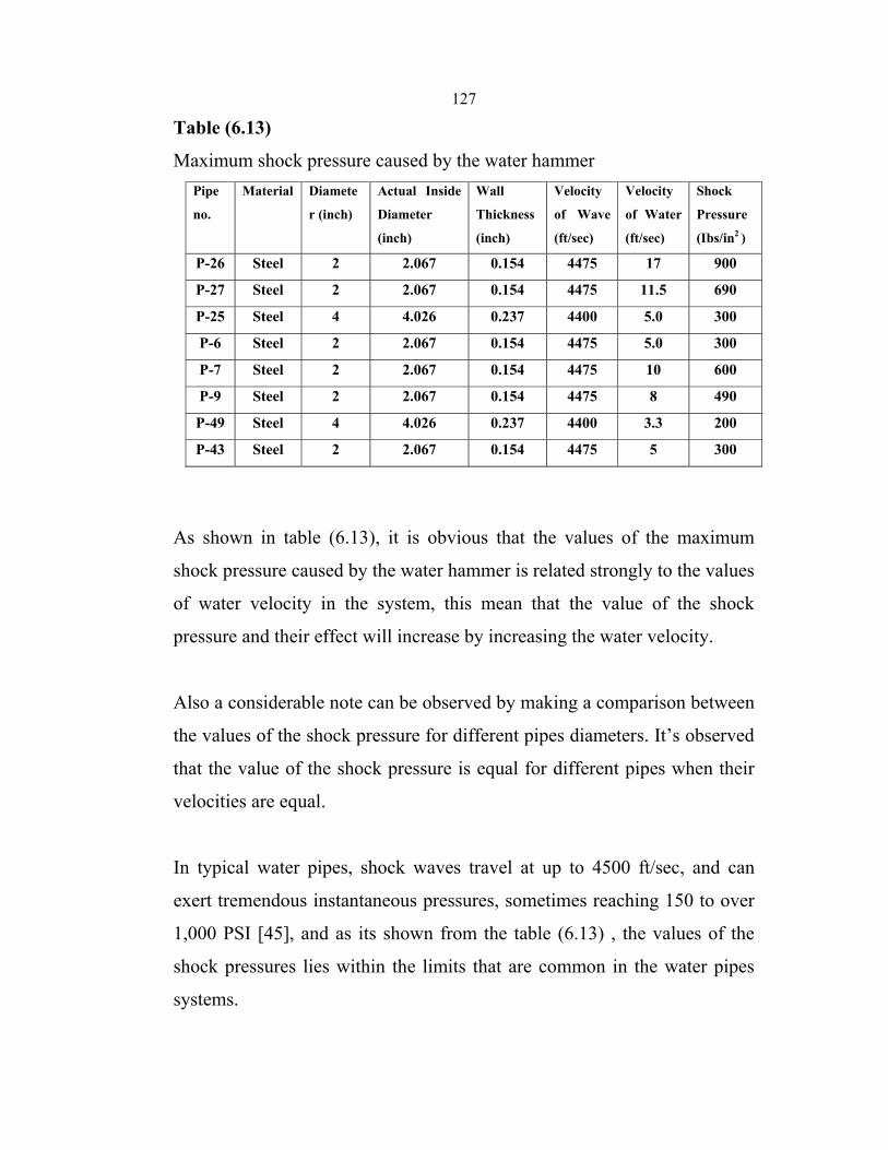
127
Table (6.13)
Maximum shock pressure caused by the water hammer Pipe
no.
Material Diamete
r (inch)
Actual Inside
Diameter
(inch)
Wall
Thickness
(inch)
Velocity
of Wave
(ft/sec)
Velocity
of Water
(ft/sec)
Shock
Pressure
(Ibs/in2 )
P-26 Steel 2 2.067 0.154 4475 17 900
P-27 Steel 2 2.067 0.154 4475 11.5 690
P-25 Steel 4 4.026 0.237 4400 5.0 300
P-6 Steel 2 2.067 0.154 4475 5.0 300
P-7 Steel 2 2.067 0.154 4475 10 600
P-9 Steel 2 2.067 0.154 4475 8 490
P-49 Steel 4 4.026 0.237 4400 3.3 200
P-43 Steel 2 2.067 0.154 4475 5 300
As shown in table (6.13), it is obvious that the values of the maximum
shock pressure caused by the water hammer is related strongly to the values
of water velocity in the system, this mean that the value of the shock
pressure and their effect will increase by increasing the water velocity.
Also a considerable note can be observed by making a comparison between
the values of the shock pressure for different pipes diameters. It’s observed
that the value of the shock pressure is equal for different pipes when their
velocities are equal.
In typical water pipes, shock waves travel at up to 4500 ft/sec, and can
exert tremendous instantaneous pressures, sometimes reaching 150 to over
1,000 PSI [45], and as its shown from the table (6.13) , the values of the
shock pressures lies within the limits that are common in the water pipes
systems.

128
Chapter Seven
Results and Discussion
7.1 Results and discussion of the intermittent model
The discussion of results which are produced by the modeling of Jenin
water distribution system as an intermittent supply systems depends on
some facts about the behavior of the Jenin water supply system under these
conditions of providing water for consumers, taking into consideration
some theoretical assumptions about the intermittent water systems.
- The modeling of the system as an intermittent system shows a high
service values of pressure up to 13 bar, which is a characteristic of
the intermittent water systems .The highest value of pressure was
recorded at the node (J-1) with a value of 12.85 bar as shown in
figure (7.1). This point of demand located below the reservoir no.1
(AL-Gabriat Reservoir), with a high difference of level up to (130
meter). Such high values of pressures are registered at nodes (J-8, J-
20, J-40), and presented in figures (7.2), (7.3), (7.4). These nodes of
demand located at different locations in the distribution system.
- When an evaluation between the pressure values at the nodes
illustrated in figures (7.1), (7.2), (7.3), (7.4) has been done, it is
noticeable that the decreasing of pressure at the nodes faraway from
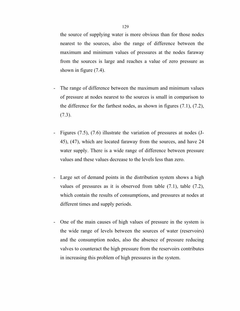
129
the source of supplying water is more obvious than for those nodes
nearest to the sources, also the range of difference between the
maximum and minimum values of pressures at the nodes faraway
from the sources is large and reaches a value of zero pressure as
shown in figure (7.4).
- The range of difference between the maximum and minimum values
of pressure at nodes nearest to the sources is small in comparison to
the difference for the farthest nodes, as shown in figures (7.1), (7.2),
(7.3).
- Figures (7.5), (7.6) illustrate the variation of pressures at nodes (J-
45), (47), which are located faraway from the sources, and have 24
water supply. There is a wide range of difference between pressure
values and these values decrease to the levels less than zero.
- Large set of demand points in the distribution system shows a high
values of pressures as it is observed from table (7.1), table (7.2),
which contain the results of consumptions, and pressures at nodes at
different times and supply periods.
- One of the main causes of high values of pressure in the system is
the wide range of levels between the sources of water (reservoirs)
and the consumption nodes, also the absence of pressure reducing
valves to counteract the high pressure from the reservoirs contributes
in increasing this problem of high pressures in the system.

130
- It is obvious from the tables (7.1), (7.2) that the high values of
pressure appear at the nodes nearest to the sources of water, and/or
have a clearly difference of levels. Also they have a 24 water supply
services.
- The values of pressure at the consumption nodes are not fixed, and
varying with time, because the demand pattern, which has been
adopted in modeling the intermittent supply system, is not fixed, and
represents the demand at the roof tank. The losses and demands at
the system are varying with time due to the demand pattern also.
- The change setting valves in the distribution system to provide the
needed amounts of water to the consumers affects the values of
pressure in the system, and the closing valves cause increasing the
pressure in the system by decreasing the losses in the system.
- These high values of pressure may affect adversely the hydraulic
performance of the water distribution network. Also they produce
high velocities, which accelerate the deterioration and corrosion of
the pipes in the distribution system.
- For the parts of the system that are located faraway from the sources,
or have high elevation, it is clearly obvious that they are suffering
from low-pressure values or even zero values of pressure. This
emphasizes the hypothesis, which state that there is a wide range of
variations in pressure values in the intermittent systems.

131
- The normal pressure values in residential areas ranges between 3.0-
4.0 bars. This means that the 12.85 bars recorded at Junction (J-1) at
time 3 hr. after the beginning of the supply period is about 3.67 times
the normal pressure value in a distribution system. Thus the network
will be under excessive pressure during the period of supply and will
release to zero pressure during non-supply periods, and this type of
loading will affect the life of pipes and increase the leakage and
breakage rates.
- When a comparison between the demand figures and the pressure
progress has been done, it is concluded that when the demand values
increase, there will be a decrease in pressure values as shown in
figures (7.7), (7.8), which illustrate the demand and pressure at the
nodes (J-29). This is because, the increasing of losses and demand in
the distribution system will decrease the values of pressure.
- The local service pressures have a certain influence on demands and
losses in the network. Higher pressures lead to increase consumption
and losses, and vice versa. Also it is reasonable to conclude that the
consumer faraway from the supply points will need to be more
patient because the refilling of their roof tanks will start later and go
slower than for those nearest to the sources points.
- The negative or zero values of pressures at the consumption nodes as
shown in table (7.1), (7.2), is an indication of presence control for
the pipes supplying these nodes at this moment, e.g., the

132
consumption nodes (J-6), and (J-7) are closed at time 12 hr and will
be open at time 24 hr, that cause zero value of pressures at this time.
- The zero values of discharges in the pipes as shown in tables (7.3),
(7.4), which illustrate the discharges and velocities in the pipes at
different times of supplying water, are also indicate to the presence
of control for the pipes at this moment. It is obvious at the pipes (P-
6), (P-7) at time 12 hr., which providing the water for junctions (J-6)
and (J-7) respectively.
- The negative sign of discharges as shown in tables (7.3) and (7.4) is
an indication to the wrong in assuming direction of flow through
pipes in the distribution system.
- When a comparison has been done between the outputs of the
intermittent model and the available field measurements which have
been done by a consultant, some of similarity can be observed as its
shown in figures (7.9), (7.10), which illustrate the pressure versus
time at Junction (J-49) (This consumption node represents Sabah
AL-Khair district).
- Generally the outputs of the intermittent model match to some level
of accurate with the field measurements which have been done by a
consultant from the point view, that the system showing high
pressures, and the farthest regions suffering from low pressures, but
the complexity of understanding the procedure of managing and
operating the Jenin water distribution system, repeated shortcuts of
supplying water to the consumers, and the continuous modification

133
and changing of the supplying intervals will appear differences
between the field measurements and the theoretical results of
modeling the system as intermittent system.
- The intermittent model shows high values of velocities, and this
result is a suspected outcome of the intermittent systems due to the
high pressures in the system. The largest registered velocity is 12.18
m/s at Junction (J-26), and this value is larger than the design values
of velocities (1.2 m/s –2.0 m/s), which are used to determine the
most economic diameters by (10.15-6.09) times, and at the same
time it’s larger than the absolute minimum velocities (0.1 m/s – 0.3
m/s), that have to be avoided in order to avoid stagnation and water
quality problems in the water systems by (121.8 – 40.6) times. These
high velocities will affect adversely causing pipes deterioration.

134 Table (7.1) Results of Consumptions and Pressures at Nodes, Time : 12 hr, Intermittent Model Node Label Elevation (m) Demand (l/s)
Calculated Demand (l/s) Hydraulic Grade (m) Pressure (m H2O)
J-1 140 1.5 2.16 259.2 118.903 J-2 145 1.12 1.613 256.35 111.073 J-3 155 2.3 3.312 255.79 100.538 J-4 165 1 1.44 252.84 87.614 J-5 150 1 1.44 254.66 104.396 J-6 140 2.4 3.456 0.00 0.00 J-7 160 3.5 5.04 0.00 0.00 J-8 150 1 1.44 254.62 104.352 J-9 170 0.45 0.648 253.28 83.067 J-10 170 6.9 9.936 252.87 82.662 J-11 175 1.62 2.333 246 70.821 J-12 160 2.76 3.974 228.52 68.345 J-13 140 1.2 1.728 245.64 105.372 J-14 145 0.45 0.648 244.84 99.584 J-15 130 5.8 8.352 243.15 112.866 J-16 180 3.8 5.472 236.74 56.598 J-17 180 0.91 1.31 233.2 53.061 J-18 131 0.73 1.051 231.87 100.614 J-19 124 1.93 2.779 223.44 99.192 J-20 118 0.723 1.041 217.28 99.03 J-21 160 0.574 0.827 216.02 55.879 J-22 190 0.815 1.174 210.77 20.722 J-23 190 0.45 0.648 210.68 20.626 J-24 140 0.352 0.507 209.76 69.585 J-25 145 3.3 4.752 156.02 10.988 J-26 115 5.8 8.352 0 0 J-27 90 10.8 15.552 0.00 0.00 J-28 137 2.3 3.312 233.14 95.901 J-29 135 0.54 0.778 227.48 92.248 J-30 180 0.67 0.965 225.8 45.688 J-31 145 1.6 2.304 194.98 49.857 J-32 145 0.815 1.174 190.97 45.851 J-33 138 0.74 1.066 192.97 54.835 J-34 150 3.41 4.91 191.03 40.931 J-35 164 3.315 4.774 163.45 -0.553 J-36 150 2.37 3.413 0.00 0.00 J-37 140 0.73 1.051 163.04 22.983

135
Table (7.1)(continue)
Node Label Elevation (m) Demand (l/s)
Calculated Demand (l/s) Hydraulic Grade (m) Pressure (m H2O)
J-38 125 0.73 1.051 160.16 35.07 J-39 115 1 1.44 142.41 27.343 J-40 108 1 1.44 130.69 22.628 J-41 132 2.74 3.946 0.00 0.00 J-42 130 1.26 1.814 0.00 0.00 J-43 132 2.4 3.456 0.00 0.00 J-44 110 1.2 1.728 0.00 0.00 J-45 138 2.3 3.312 127.88 -10.093 J-46 132 3.25 4.68 55.22 -76.582 J-47 130 2.5 3.6 86.92 -42.967 J-48 134 12.9 18.576 68.73 -65.101 J-49 132 3.6 5.184 78.78 20.207 J-50 165 3.5 5.04 237.48 72.302 J-51 210 2.3 3.312 235.99 25.921 J-53 240 0.5 0.72 272.18 32.096 J-52 237 1.5 2.16 272.13 35.044 J-54 238 1.5 2.16 271.91 33.819 J-55 232 1.5 2.16 271.83 39.732 J-56 235 0.7 1.008 0.00 0.00 J-57 260 0.7 1.008 0.00 0.00 J-58 250 0.7 1.008 0.00 0.00 228 215 0.7 1.008 0.00 0.00 J-60 226 0.67 0.965 0.00 0.00

136
Table (7.2) Results of Consumptions and Pressures at Nodes, Time :24 hour, Intermittent Model Node Label Elevation (m) Demand (l/s)
Calculated Demand (l/s) Hydraulic Grade (m) Pressure (m H2O)
J-1 140 1.5 0.945 267.72 127.396J-2 145 1.12 0.706 267.1 121.793J-3 155 2.3 1.449 266.98 111.696J-4 165 1 0.63 266.34 101.083J-5 150 1 0.63 266.73 116.439J-6 140 2.4 1.512 261.6 121.293J-7 160 3.5 2.205 256.42 96.172J-8 150 1 0.63 266.72 116.429J-9 170 0.45 0.283 266.43 96.191J-10 170 6.9 4.347 0.00 0.00J-11 175 1.62 1.021 0.00 0.00J-12 160 2.76 1.739 261.07 100.814J-13 140 1.2 0.756 257.2 116.902J-14 145 0.45 0.283 257.02 111.741J-15 130 5.8 3.654 0.00 0.00J-16 180 3.8 2.394 247.71 67.541J-17 180 0.91 0.573 246.94 66.775J-18 131 0.73 0.46 240.65 109.372J-19 124 1.93 1.216 238.82 114.533J-20 118 0.723 0.455 237.49 119.186J-21 160 0.574 0.362 237.21 77.02J-22 190 0.815 0.513 236.08 45.962J-23 190 0.45 0.283 236.06 45.941J-24 140 0.352 0.222 235.86 95.616J-25 145 3.3 2.079 224.21 79.013J-26 115 5.8 3.654 58.82 -56.035J-27 90 10.8 6.804 -44.88 -134.544J-28 137 2.3 1.449 240 102.735J-29 135 0.54 0.34 239.47 104.207J-30 180 0.67 0.422 239.11 58.958J-31 145 1.6 1.008 232.43 87.208J-32 145 0.815 0.513 231.56 86.34J-33 138 0.74 0.466 231.99 93.756J-34 150 3.41 2.148 231.57 81.367J-35 164 3.315 2.088 225.6 61.44J-36 150 2.37 1.493 221.08 70.902J-37 140 0.73 0.46 225.51 85.292J-38 125 0.73 0.46 224.88 99.631J-39 115 1 0.63 221.04 105.771J-40 108 1 0.63 218.5 110.218

137
Table (7.2) (continue)
Node Label Elevation (m) Demand (l/s)
Calculated Demand (l/s) Hydraulic Grade (m) Pressure (m H2O)
J-41 132 2.74 1.726 218.22 85.999 J-42 130 1.26 0.794 155.18 25.112 J-43 132 2.4 1.512 217.1 84.887 J-44 110 1.2 0.756 215.32 105.056 J-45 138 2.3 1.449 217.89 79.688 J-46 132 3.25 2.047 202.15 69.969 J-47 130 2.5 1.575 209.01 78.816 J-48 134 12.9 8.127 205.07 70.894 J-49 132 3.6 2.268 207.25 0 J-50 165 3.5 2.205 239.99 74.802 J-51 210 2.3 1.449 239.67 29.592 J-53 240 0.5 0.315 273.76 33.671 J-52 237 1.5 0.945 273.75 36.654 J-54 238 1.5 0.945 273.7 35.608 J-55 232 1.5 0.945 273.68 41.577 J-56 235 0.7 0.441 155.17 -79.633 J-57 260 0.7 0.441 155.08 -104.655 J-58 250 0.7 0.441 154.97 -94.79 228 215 0.7 0.441 154.96 -59.886 J-60 226 0.67 0.422 154.96 -70.86

138
Table (7.3) Pipes, Lengths, Discharges, and Velocities, Time :12 hr, Intermittent Model Link Label
Length (m)
Diameter (in) Material
Initial Status
Current Status
Discharge (l/s)
Headloss (m) Velocity (m/s)
P-54 168 10 Steel Open Open 83.183 2.82 1.70 P-2 230 6 Steel Open Open 18.389 2.85 1.04 P-10 150 4 Steel Open Open 12.269 6.33 1.56 P-12 200 2 Steel Open Open 3.974 30.69 2.02 P-13 270 6 Steel Open Open 39.191 13.57 2.22 P-3 150 4 Steel Open Open 3.312 0.56 0.42 P-4 150 2 Steel Open Open 1.44 3.52 0.73 P-5 300 6 Steel Open Open 12.024 1.69 0.68 P-6 200 2 Steel Open Closed 0 0 0.00 P-7 200 2 Steel Open Closed 0 0 0.00 P-8 200 6 Steel Open Open 2.088 0.04 0.12 P-9 250 2 Steel Open Open 0.648 1.34 0.33 P-11 120 2 Steel Open Open 2.333 6.87 1.19 P-14 150 2 Steel Open Open 0.648 0.8 0.33 P-15 120 4 Steel Open Open 8.352 2.49 1.06 P-16 320 6 Steel Open Open 28.463 8.9 1.61 P-17 180 2 Steel Open Open 1.31 3.55 0.67 P-18 290 6 Steel Open Open 21.68 4.87 1.23 P-19 200 6 Steel Open Open 35.631 8.43 2.02 P-28 150 6 Steel Open Open -15.002 1.28 -0.85 P-20 170 6 Steel Open Open 32.852 6.16 1.86 P-21 150 2 Steel Open Open 0.827 1.26 0.42 P-22 200 6 Steel Open Open 30.984 6.51 1.75 P-23 180 4 Steel Open Open 1.155 0.1 0.15 P-25 270 4 Steel Open Open 28.656 54.76 3.65 P-24 270 2 Steel Open Open 0.507 0.92 0.26 P-26 180 2 Steel Open Open 23.904 763.31 12.18 P-27 250 2 Steel Open Open 15.552 478.63 7.92 P-51 250 8 Steel Open Open -47.059 4.34 -1.50 P-29 200 6 Steel Open Open 28.745 5.66 1.63 P-30 150 2 Steel Open Open 0.965 1.68 0.49 P-32 200 6 Steel Open Open 73.915 32.5 4.18 P-31 250 6 Steel Open Open 46.913 17.52 2.66 P-33 250 2 Steel Open Open 1.174 4.02 0.60 P-34 180 4 Steel Open Open 5.976 2.01 0.76 P-36 250 6 Steel Open Open 64.462 31.54 3.65 P-35 250 4 Steel Open Open 4.91 1.94 0.63 P-37 180 2 Steel Open Closed 0 0 0.00 P-38 250 4 Steel Open Open 2.102 0.4 0.27 P-40 230 6 Steel Open Open 54.173 21.03 3.07

139
Table (7.3) (continue)
Link Label
Length (m)
Diameter (in) Material
Initial Status
Current Status
Discharge (l/s)
Headloss (m)
Velocity (m/s)
P-39 220 2 Steel Open Open 1.051 2.88 0.54 P-41 500 2 Steel Open Open 1.44 11.73 0.73 P-42 190 4 Steel Open Closed 0 0 0.00 P-46 350 6 Steel Open Open 35.352 14.53 2.00 P-43 700 2 Steel Open Open 6.811 290.17 3.47 P-44 600 4 Steel Open Open 5.184 4.88 0.66 P-60 62 6 Ductile Iron Open Open 4.997 1.22 0.28 P-45 250 2 Steel Open Open 1.728 8.53 0.88 P-47 350 2 Steel Open Open 4.68 72.66 2.38 P-48 220 4 Steel Open Open 27.36 40.96 3.49P-49 200 4 Steel Open Open 18.576 18.19 2.37 P-50 950 4 Steel Open Open 5.184 8.15 0.66 P-52 400 4 Steel Open Open 3.312 1.5 0.42P-55 913 10 Steel Open Open 75.983 12.97 1.55 P-57 488 10 Ductile Iron Open Open 6.48 0.04 0.13 P-56 174 8 Ductile Iron Open Open 55.411 2.52 1.76 P-58 435 6 Ductile Iron Open Open 4.32 0.23 0.24 P-59 500 6 Ductile Iron Open Open 2.16 0.07 0.12 P-61 121 4 Ductile Iron Open Open 3.989 0 0.51 P-62 268 4 Ductile Iron Open Open 2.981 0 0.38 P-63 41 4 Ductile Iron Open Open 1.973 0 0.25 P-64 42 4 Ductile Iron Open Open 0.965 0 0.12

140
Table (7.4) Pipes, Lengths, Discharges , and Velocities , Time :24 hour, Intermittent Model
Link Label
Length (m)
Diameter (in) Material
Initial Status
Current Status
Discharge (l/s)
Headloss (m)
Velocity (m/s)
P-54 168 10 Steel Open Open 53.406 1.24 1.1 P-2 230 6 Steel Open Open 8.045 0.62 0.5 P-10 150 4 Steel Open Closed 0 0 0.0 P-12 200 2 Steel Open Open 1.739 6.65 0.9 P-13 270 6 Steel Open Open 34.159 10.52 1.9 P-3 150 4 Steel Open Open 1.449 0.12 0.2 P-4 150 2 Steel Open Open 0.63 0.76 0.3 P-5 300 6 Steel Open Open 5.26 0.37 0.3 P-6 200 2 Steel Open Open 2.91 5.13 1.5 P-7 200 2 Steel Open Open 5.90 10.32 3.0 P-8 200 6 Steel Open Open 0.913 0.01 0.1 P-9 250 2 Steel Open Open 5.0 0.29 2.5 P-11 120 2 Steel Open Open 1.021 1.22 0.5 P-14 150 2 Steel Open Open 0.283 0.17 0.1 P-15 120 4 Steel Open Closed 0 0 0.0 P-16 320 6 Steel Open Open 29.466 9.49 1.7 P-17 180 2 Steel Open Open 0.573 0.77 0.3 P-18 290 6 Steel Open Open 26.498 7.06 1.5 P-19 200 6 Steel Open Open 15.589 1.83 0.9 P-28 150 6 Steel Open Open 10.45 0.65 0.6 P-20 170 6 Steel Open Open 14.373 1.34 0.8 P-21 150 2 Steel Open Open 0.362 0.27 0.2 P-22 200 6 Steel Open Open 13.556 1.41 0.8 P-23 180 4 Steel Open Open 0.505 0.02 0.1 P-25 270 4 Steel Open Open 12.537 11.86 1.6 P-24 270 2 Steel Open Open 0.222 0.2 0.1 P-26 180 2 Steel Open Open 10.458 165.39 5.3 P-27 250 2 Steel Open Open 6.804 103.71 3.5 P-51 250 8 Steel Open Open 1.054 3.90E-03 0.0 P-29 200 6 Steel Open Open 7.947 0.52 0.4 P-30 150 2 Steel Open Open 0.422 0.36 0.2 P-32 200 6 Steel Open Open 32.338 7.04 1.8 P-31 250 6 Steel Open Open 25.153 5.53 1.4 P-33 250 2 Steel Open Open 0.513 0.87 0.3 P-34 180 4 Steel Open Open 2.615 0.44 0.3 P-36 250 6 Steel Open Open 28.202 6.83 1.6 P-35 250 4 Steel Open Open 2.148 0.42 0.3 P-37 180 2 Steel Open Open 1.493 4.51 0.8 P-38 250 4 Steel Open Open 0.92 0.09 0.1 P-40 230 6 Steel Open Open 23.701 4.56 1.3

141
Table (7.4) (continue)
Link
Label Length
(m) Diameter
(in) Material Initial Status
Current Status
Discharge (l/s)
Headloss (m)
Velocity (m/s)
P-39 220 2 Steel Open Open 0.46 0.62 0.2 P-41 500 2 Steel Open Open 0.63 2.54 0.3 P-42 190 4 Steel Open Open 6.974 2.82 0.9 P-46 350 6 Steel Open Open 15.466 3.15 0.9 P-43 700 2 Steel Open Open 2.98 63.04 1.5 P-44 600 4 Steel Open Open 2.268 1.12 0.3 P-60 62 6 Ductile Iron Open Open 2.186 0.01 0.1 P-45 250 2 Steel Open Open 0.756 1.78 0.4 P-47 350 2 Steel Open Open 2.047 15.74 1.0 P-48 220 4 Steel Open Open 11.97 8.87 1.5 P-49 200 4 Steel Open Open 8.127 3.94 1.0 P-50 950 4 Steel Open Open 2.268 1.77 0.3 P-52 400 4 Steel Open Open 1.449 0.32 0.2 P-55 913 10 Steel Open Open 50.256 6.04 1.0 P-57 488 10 Ductile Iron Open Open 2.835 0.01 0.1 P-56 174 8 Ductile Iron Open Open 2.6 0.01 0.1 P-58 435 6 Ductile Iron Open Open 1.89 0.05 0.1 P-59 500 6 Ductile Iron Open Open 0.945 0.02 0.1 P-61 121 4 Ductile Iron Open Open 1.745 0.09 0.2 P-62 268 4 Ductile Iron Open Open 1.304 0.11 0.2 P-63 41 4 Ductile Iron Open Open 0.863 0.01 0.1 P-64 42 4 Ductile Iron Open Open 0.422 2.10E-03 0.1

142
Figure (7.1) Pressure versus Time at Junction: J –1
Pressure varying TimeJunction: J-1
Time(hr)
(m H
2O)
Pre
ssur
e
116.0
118.0
120.0
122.0
124.0
126.0
128.0
130.0
0.0 10.0 20.0 30.0 40.0 50.0 60.0 70.0 80.0
Base

143
Figure (7.2) Pressure versus Time at Junction: J-8
Pressure varying TimeJunction: J-8
Time(hr)
(m H
2O
)P
ress
ure
100.0
102.0
104.0
106.0
108.0
110.0
112.0
114.0
116.0
118.0
120.0
0.0 10.0 20.0 30.0 40.0 50.0 60.0 70.0 80.0
Base
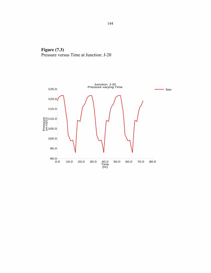
144
Figure (7.3) Pressure versus Time at Junction: J-20
Pressure varying TimeJunction: J-20
Time(hr)
(m H
2O
)P
ress
ure
90.0
95.0
100.0
105.0
110.0
115.0
120.0
125.0
0.0 10.0 20.0 30.0 40.0 50.0 60.0 70.0 80.0
Base

145
Figure (7.4) Pressure versus Time at Junction: J-40
Pressure varying TimeJunction: J-40
Time(hr)
(m H
2O
)P
ress
ure
-20.0
0.0
20.0
40.0
60.0
80.0
100.0
120.0
140.0
0.0 10.0 20.0 30.0 40.0 50.0 60.0 70.0 80.0
Base

146
Figure (7.5) Pressure versus Time at Junction: J-45
Pressure varying TimeJunction: J-45
Time(hr)
(m H
2O
)P
ress
ure
-40.0
-20.0
0.0
20.0
40.0
60.0
80.0
100.0
0.0 10.0 20.0 30.0 40.0 50.0 60.0 70.0 80.0
Base

147
Figure (7.6) Pressure versus Time at Junction: J-47
Pressure varying TimeJunction: J-47
Time(hr)
(m H
2O
)P
ress
ure
-80.0
-60.0
-40.0
-20.0
0.0
20.0
40.0
60.0
80.0
100.0
0.0 10.0 20.0 30.0 40.0 50.0 60.0 70.0 80.0
Base

148
Figure (7.7) Demand versus Time at Junction: J-29
Demand varying TimeJunction: J-29
Time(hr)
(l/s
)D
em
an
d
0.2
0.3
0.4
0.5
0.6
0.7
0.8
0.9
0.0 10.0 20.0 30.0 40.0 50.0 60.0 70.0 80.0
Base

149
Figure (7.8) Pressure versus Time at Junction: J-29
Pressure varying TimeJunction: J-29
Time(hr)
(m H
2O
)P
ress
ure
88.0
90.0
92.0
94.0
96.0
98.0
100.0
102.0
104.0
106.0
0.0 10.0 20.0 30.0 40.0 50.0 60.0 70.0 80.0
Base

150
Figure (7.9) Pressure versus Time at Junction: J-49
Pressure varying TimeJunction: J-49
Time(hr)
(m H
2O
)P
ress
ure
0.0
5.0
10.0
15.0
20.0
25.0
0.0 10.0 20.0 30.0 40.0 50.0 60.0 70.0 80.0
Base

151
Figure (7.10) Pressure measurement versus Time (Field measurement) at Junction: J-49
Time
Pressure (bar)

152
7.2 Results and discussion of the continuous model
The results of continuous model of Jenin water distribution network discuss
the ability of the existing system with the assumed assumptions and
development measures such as the availability of water, increasing of
demand, reducing the losses and high pressures, to satisfy the requirements
of demands, limits of velocities and pressures in order to provide the water
by acceptable quantity and quality in the future.
The comparison of results of analysis the proposed model of continuous
supply with the assumed limits of velocities which have been established to
be 0.1-0.3 m/s. (minimum velocities), and represent the absolute minimum
velocities that have to be avoided in order to avoid stagnation and water
quality problems, the limits of maximum pressures were set at 6 bar and the
minimum pressure for the main lines at 0.5 bar shows the following:
- It is obvious from the table (7.5), that the high values of pressure
appear at the nodes nearest to the sources of water or booster stations
as its shown in the intermittent systems which lead also to conclude
that the consumer faraway from the supply points will need to be
more patient, some high values of pressure are specified at the nodes
(J-85: 5.6 bar, J-86: 6.2 bar, J-87: 8 bar, J-88: 6.7 bar, J-29: 8.3 bar,
J-28: 8.2 bar, J-42: 8 bar).
- The demand nodes which are faraway from the sources or booster
stations and have high levels suffer from low pressure values as its
shown in table (7.5), and registered for example at the nodes (J-27 :

153
0.35 bar, J-49 : 1.6 bar, J-44 : 0.4 bar, J-46 : 1.4 bar, J-69 : 0.56 bar,
J-70 : 0.46 bar).
- The results of the pressure values in the whole system as it is
mentioned in the table (7.5), show the ability of the system to satisfy
the needed pressures that are necessary with some extreme values
neither smaller or larger than the specified values of pressure, and
this conclusion lead to suggest the capability of the system to serve
the people in the future in the case of adding some developing
measures such as, providing the necessary quantities of water, using
booster stations in the hill areas , and controlling the high pressures
in the system.
- The results of the pressure values in the continuous system show the
valuable of using pressure reducing valves to counteract the high
pressure from the reservoirs and limit the pressures in the system to
the specified or needed values. This way of manage the system will
affect positively the hydraulic performance of the distribution
network, especially that it will reduce the losses and velocities in the
system and consequently reduce the adverse effects of the high
velocities which cause deterioration of the pipes in the system, and
save the water meter of the customers from blowing up due to the
high pressures.
- The results of velocities in the continuous system as shown in table
(7.6) appear a reasonable values of velocities, which are parallel to
the assumed limits of velocities to avoid stagnation and quality water

154
problems, also to save the pipes from deterioration due to the high
velocities.
- The negative sign of the discharges in the pipes as shown in table
(7.6) is an indication to the wrong in assuming direction only.

155
Table (7.5) Results of Consumptions and Pressures at Nodes, Steady State Analysis, Continuous Model
Node Label Elevation (m) Demand (l/s) Hydraulic Grade (m) Pressure (m H2O) J-1 140 2.83 200.13 59.981 J-2 145 2.5323 196.6 51.47 J-3 155 3.713 195.91 40.803 J-4 165 2.3355 187.99 22.936 J-5 150 2.3355 194.89 44.781 J-6 140 2.5323 181.57 41.461 J-7 160 3.1226 175.25 15.216 J-8 150 2.3355 194.74 44.629 J-9 170 1.745 186.38 16.334 J-10 170 3.713 198.67 28.598 J-11 175 1.844 194.22 19.174 J-12 160 4.205 166.07 6.057 J-13 140 2.533 200.82 60.67 J-14 145 1.7453 195.8 50.674 J-15 130 3.32 200.37 70.195 J-16 180 5.29 203.69 23.632 J-17 180 2.24 194.13 14.096 J-18 131 2.04 209.11 77.916 J-19 124 3.32 205.87 81.665 J-20 118 2.04 203.86 85.642 J-21 160 1.883 198.08 37.984 J-22 190 2.14 202.36 12.327 J-23 190 1.75 201.65 11.621 J-24 140 1.65 193.5 53.369 J-25 145 2.04 196.6 51.472 J-26 115 2.63 129.15 14.119 J-27 90 3.81 93.68 3.671 J-28 137 3.7148 219.36 82.152 J-29 135 1.8436 218.3 83.086 J-30 180 1.9814 211.95 31.865 J-31 145 2.92581 195.48 50.352 J-32 145 2.1388 183.29 38.192 J-33 138 2.04 192.83 54.697 J-34 150 4.8934 190.91 40.804 J-35 164 4.795 176.45 12.421 J-36 150 2.5323 164.46 14.42 J-37 140 2.0404 175.07 34.986 J-38 125 2.0404 165.24 40.141 J-39 115 2.3355 165.72 50.597 J-40 108 2.3355 137.03 28.962 J-41 132 2.73 153.8 21.746 J-42 130 0.35 209.98 79.781 J-43 132 1.9 147.84 15.799 J-44 110 3.713 114.02 4.008 J-45 138 3.713 161.65 23.592 J-46 132 2.04 146.02 13.98

156
Table (7.5) (continue) Node Label
Elevation (m) Demand (l/s) Hydraulic Grade (m) Pressure (m H2O)
J-45 138 3.713 161.65 23.592 J-46 132 2.04 146.02 13.98 J-47 130 3.91 152.71 22.649 J-48 134 4.3 151.49 17.448 J-49 132 3.812 148.09 16.051 J-50 165 4.952 225.08 59.927 J-51 210 3.7148 223.23 13.193 J-53 240 0.5824 273.31 33.228 J-52 237 0.212 277.26 40.155 J-54 238 0.212 277.21 39.106 J-55 232 0.212 277.08 44.963 J-56 235 0.212 276.97 41.868 J-57 260 0.27 276.88 16.842 J-58 250 0.27 276.87 26.797 J-59 253 0.27 276.85 23.789 J-60 256 0.27 276.8 20.752 J-61 266 0.2683 276.75 10.726 J-62 266 0.2683 276.74 10.713 J-63 268 0.2683 276.73 8.708 J-64 270 0.2683 276.71 6.693 J-65 265 0.2683 276.7 11.67 J-66 265 0.2683 276.69 11.664 J-67 270 0 276.69 6.676 J-68 266 0.2683 276.69 10.664 J-69 271 0.2683 276.69 5.674 J-70 272 0.2683 276.69 4.677 J-71 250 0.2683 276.69 26.621 J-72 255 0.2683 276.69 21.638 J-73 257 0.2683 276.69 19.642 J-74 257 0.2683 276.69 19.642 J-75 260 0.2683 276.69 16.65 J-76 172 0.8968 209.91 37.818 J-77 177 0.8968 209.17 32.093 J-78 185 0.8968 207.99 22.93 J-79 200 0.8968 207.86 7.845 J-80 202 0.9 207.79 5.774 J-81 202 0.9 207.57 5.553 J-82 190 0.4 205.76 15.716 J-83 192 0.36 205.1 13.072 J-84 177 0.36 204.74 27.674 J-85 217 1.1 273.15 56.013 J-86 211 2.49 273.07 61.915 J-87 193 2.1 273.02 79.814 J-88 206 2 272.99 66.826 J-89 246 0.3 272.51 26.446 J-90 259 2.1 272.36 13.322 J-91 246 0.6 272.46 26.392 J-92 200 2.1 272.32 72.142

157
Table (7.6) Pipes,Lengths,Discharges,and Velocities, Steady State Analysis, Continuous Model Link Label
Length (m)
Diameter (in) Material
Initial Status
Discharge (l/s)
Headloss (m)
Velocity ( m/s)
P-54 168 10 Steel Open 38.77791 0.69 0.79 P-2 230 6 Steel Open 20.6517 3.53 1.17 P-10 150 4 Steel Open 5.557 1.46 0.71 P-12 200 2 Steel Open 4.205 34.06 2.14 P-13 270 6 Steel Open -7.83819 0.69 0.44 P-3 150 4 Steel Open 3.713 0.69 0.47 P-4 150 2 Steel Open 2.3355 8.61 1.19 P-5 300 6 Steel Open 12.0709 1.71 0.68 P-6 200 2 Steel Open 2.5323 13.33 1.29 P-7 200 2 Steel Open 3.1226 19.64 1.59 P-8 200 6 Steel Open 4.0805 0.15 0.23 P-9 250 2 Steel Open 1.745 8.37 0.89 P-11 120 2 Steel Open 1.844 4.45 0.94 P-14 150 2 Steel Open 1.7453 5.02 0.89 P-15 120 4 Steel Open 3.32 0.45 0.42 P-16 320 6 Steel Open -15.43649 2.87 0.87 P-17 180 2 Steel Open 2.24 9.56 1.14 P-18 290 6 Steel Open -22.96649 5.42 1.30 P-19 200 6 Steel Open 21.263 3.24 1.20 P-28 150 6 Steel Open -46.26949 10.25 2.60 P-20 170 6 Steel Open 17.943 2.01 1.02 P-21 150 2 Steel Open 1.883 5.78 0.96 P-22 200 6 Steel Open 14.02 1.5 0.79 P-23 180 4 Steel Open 3.4 0.71 0.43 P-25 270 4 Steel Open 8.48 5.76 1.08 P-24 270 2 Steel Open 1.65 8.15 0.84 P-26 180 2 Steel Open 6.44 67.45 3.28 P-27 250 2 Steel Open 3.81 35.47 1.94 P-51 200 8 Steel Open -61.62719 5.72 1.96 P-29 200 6 Steel Open 11.6429 1.06 0.66 P-30 150 2 Steel Open 1.9814 6.35 1.01 P-32 200 6 Steel Open 61.0523 22.82 3.46 P-99 87.5 6 PVC Open 5.6842 0.06 0.32 P-31 250 6 Steel Open 58.91861 26.7 3.34 P-33 250 2 Steel Open 2.1388 12.19 1.09 P-34 180 4 Steel Open 6.9334 2.64 0.88 P-36 250 6 Steel Open 49.0543 19.03 2.78 P-35 250 4 Steel Open 4.8934 1.93 0.62 P-37 180 2 Steel Open 2.5323 12 1.29 P-38 250 4 Steel Open 4.0808 1.38 0.52 P-40 230 6 Steel Open 37.6462 10.73 2.13 P-39 220 2 Steel Open 2.0404 9.83 1.04 P-41 500 2 Steel Open 2.3355 28.69 1.19 P-42 190 4 Steel Open 15.2002 11.92 1.94 P-46 350 6 Steel Open 17.775 4.07 1.01

158
Table (7.6) (continue)
Link Label
Length (m)
Diameter (in) Material
Initial Status
Discharge (l/s)
Headloss (m)
Velocity ( m/s)
P-44 600 4 Steel Open 5.613 5.96 0.72 P-97 125 6 Ductile Iron Open 6.85 0.15 0.39 P-80 62 6 Ductile Iron Open 6.50 0.07 0.37 P-45 250 2 Steel Open 3.713 33.82 1.89 P-47 350 2 Steel Open 2.04 15.64 1.04 P-48 220 4 Steel Open 12.02 8.95 1.53 P-49 200 4 Steel Open 4.3 1.21 0.55 P-50 950 4 Steel Open 3.812 4.61 0.49 P-52 400 4 Steel Open 3.71 1.85 0.47 P-89 488 10 Ductile Iron Open 12.79 0.16 0.26 P-101 836 10 Steel Open 25.4 1.57 0.52 P-103 173.5 8 Steel Open 70.29 6.33 2.24 P-58 82 6 PVC Open 5.47 0.05 0.31 P-59 222 6 PVC Open 5.26 0.13 0.30 P-60 192 6 PVC Open 5.04 0.1 0.29 P-61 181 6 PVC Open 4.8362 0.09 0.27 P-62 44 6 PVC Open 4.5662 0.02 0.26 P-63 40 6 PVC Open 4.2962 0.02 0.24 P-64 127 6 PVC Open 4.0262 0.04 0.23 P-65 167 6 PVC Open 3.7562 0.05 0.21 P-66 47 6 PVC Open 3.4879 0.01 0.20 P-67 44 6 PVC Open 3.2196 0.01 0.18 P-68 98 6 PVC Open 2.9513 0.02 0.17 P-69 67 6 PVC Open 2.683 0.01 0.15 P-70 40 6 PVC Open 2.4147 0.01 0.14 P-71 31 6 PVC Open 1.0732 9.50E-04 0.06 P-76 33 6 PVC Open 1.0732 1.00E-03 0.06 P-72 60 6 PVC Open 1.0732 1.80E-03 0.06 P-73 120 6 PVC Open 0.8049 2.10E-03 0.05 P-74 22 6 PVC Open 0.5366 1.90E-04 0.03 P-75 184 6 PVC Open 0.2683 4.50E-04 0.02 P-77 34 6 PVC Open 0.8049 6.00E-04 0.05 P-78 30 6 PVC Open 0.5366 2.60E-04 0.03 P-79 35 6 PVC Open 0.2683 7.40E-05 0.02 P-81 121 4 Ductile Iron Open 5.6104 0.74 0.71 P-82 268 4 Ductile Iron Open 4.7136 1.19 0.60 P-83 41 4 Ductile Iron Open 3.8168 0.12 0.49 P-84 42 4 Ductile Iron Open 2.92 0.08 0.37 P-85 239 4 Ductile Iron Open 2.02 0.22 0.26 P-86 123 2 Steel Open 1.12 1.81 0.57 P-87 100 2 Steel Open 0.72 0.65 0.37 P-88 200 2 Steel Open 0.36 0.36 0.18 P-90 300 10 Ductile Iron Open 11.69 0.08 0.24 P-91 322 10 Ductile Iron Open 9.2 0.06 0.19 P-92 411 8 Steel Open 2 0.02 0.06 P-93 435 6 Steel Open 5.1 0.5 0.29 P-94 700 6 Ductile Iron Open 2.1 0.16 0.12 P-95 151 6 Ductile Iron Open 2.7 0.05 0.15

159
Table (7.6) (continue)
Link
Label Length
(m) Diameter
(in) Material Initial Status
Discharge (l/s)
Headloss (m)
Velocity ( m/s)
P-96 601 6 Ductile Iron Open 2.1 0.13 0.12 P-98 125 6 Ductile Iron Open 6.8572 0.15 0.39
P-100 20 6 PVC Open 5.6842 0.01 0.32 P-102 10 10 Steel Open 25.40551 0.02 0.52 P-104 2 8 Steel Open 70.29399 0.07 2.24

160
Conclusions and Suggestions Conclusions:
1. For the existing situation of the Jenin water distribution system, the
following conclusions can be extracted:
- Insufficient availability of water combined with unreliability of
sources.
- Unstructured network made of old pipes.
- Excessive service pressure.
- Intermittent supply, which is directly connected to the state of
unavailability of water.
- Excessive rate of unaccounted for water.
2. The intermittent service is the procedure of providing water that is
followed in operating most of the water distribution systems in
Palestine.
3. The intermittent supply affects the hydraulic performance of the
network and exposes it to high values of pressure and velocities.
4. The designers of the water supply networks as in the case of Jenin’s
water distribution system did not consider the effects of the
intermittent supply on the value of the design factors.

161
5. There is adverse affect of the intermittent systems on the readings of
the customer water meters due to the pushed and sucked air in the
network.
6. The system shows the ability to cope the future extension in the case
of providing the necessary requirements of developing and/or
replacing the old pipes, providing the needed quantities of potable
water and overcoming the problems of high pressures by using
pressure reducing valves.

162
Suggestions and Recommendations
1. Specialized software should be developed to model the behavior of
the intermittent systems in our region.
2. More local studies are recommended. This is to understand how the
water systems in our region perform under the local conditions of
operation and management.
3. The universal peak factors which are used in the design of water
distribution systems should be modified and adjusted in the design of
new water systems in Palestine according to the local conditions of
operating and managing the distribution networks.

163
REFERENCES
1. Warren Viessman, Jr. Mark J. Hammer. (1994). “Water Supply and
Pollution Control”. Fifth Edition, Harpercolins College Publishers. 2. James E. Funk. (1994). “ Effects of Transient Operation on the
Reliability of Hydraulic Systems”. Improving Efficiency and Reliability in Water Distribution Systems. Department of Mechanical Engineering. University of Kentucky, Lexington, U.S.A.
3. Abu Madi M. (1996). “ Computer Modeling of Water
Distribution Systems With Intermittent Supply (Case Study: Tulkarm-Palestine)”, M.SC. Thesis, DELFT Institute.
4. Jarrar H. (1998). “ Evaluation of The Hydraulic Performance of
Water Distribution Systems Under The Action of Cyclic Pumping”, M.SC. Thesis, An-Najah National University.
5. Masri M. (1997). “Design of Optimal Water distribution
Networks”, M.SC. Thesis, An-Najah National University. 6. Naeeni S. (1996). “ Optimizations of Water Distribution
Networks”, Journal of Hydraulic Research, Vol.34, 1996, No.5.
7. Al-Abbase R. (2000). “Analysis and Balancing of Sectors in
Mosul’s Water Supply Networks by Using Computer”, M.SC. Thesis, Mosul University, Mosul, Iraq.
8. Ligget and Chen. (1994). “ Inverse Transient Analysis in Pipe
Networks”. Journal of Hydraulic Engineering. ASCE, Vol. (120), No.8, August, 1994.
9. Gendese, Gallerano, and Minisitti. (1987). “Multiobjective Analysis
in Optimal Solution of Hydraulic Networks”. Journal of Hydraulic Engineering. ASCE, Vol. (113), No. 9, September, 1987

164
10. Perez, Martinez, and Vela. (1993). “Improved Design of Branched Networks by Using Pressure Reducing Valves”. Journal of Hydraulic Engineering. ASCE, Vol. (119), No.2, Feb., 1993.
11. Vairavamoorthy, K., Akinpelu, E., Lin, Z., and Ali, M. (2000). “An
Appropriate Design Tool For Intermittent Water Supply Systems”, Technical Report, South Bank University, London.
12. Battermann, A. and Macke, S. (2001). “A Strategy to Reduce
Technical Water Losses for Intermittent Water Supply”. Diploma Thesis, DORSCH Consult, Germany.
13. Vairavamoorthy, K. and Lumbers, J. (1998). “Leakage Reduction
in Water Distribution Systems: Optimal Valve Control”. Journal of Hydraulic Engineering, Vol. (124), No.11, November,1998.
14. Abdel-Latif, M.Y (2001). “ Water Distribution Modeling With
Intermittent Supply: Sensitivity Analysis and Performance Evaluation For Bani Suhila City –Palestine”. M.SC. Thesis. DELFT institute.
15. Yan, J.M. (2001). “Modeling Contaminant Intrusion into Water
Distribution Systems”. Department of Civil and Building Engineering, Loughborough University, UK.
16. Saleh, A. (1999). “Internal Evaluation of Palestinian Water
Industry”. Palestinian Hydrology Group.
17. DIN ISO 4064, (1981). “Durchflussmessung von Wasser in
geschlossenen Leitungen, Zahler fur kaltes Trinkwasser, Spezifikationen, Teil 1. Technical report, Deutches Institute fur Normung, Germany.
18. Sabbah,W and Issac, J. (1995). “Towards a Palestinian Water Policy”, Applied Research Institute, Jerusalem, Palestine. 19. United Nations. (1992). “ Water Resources of The Occupied Palestinian Territory”, New York, USA.

165
20. Abu Zahr, B. (2001). “ Water Crisis in Palestine”. Elsevier Science. http://www.desline.com 21. Tahal, (1990). “ Israel Water Sector-Past Achievements, Current Problems and Future Options”. Report for the World Bank; Tahal Water Planning for Israel, Tel Aviv. 22. Abu Faris, H. (1988). “ Potential hydro-Power Production of The Dead Sea”. M.SC. Thesis, University of Jordan, Amman. 23. Nuseibeh, M and Nasser Eddin, T. (1995). “Palestinian Fresh Water Springs: Spring Description, Flow and Water Quality Data 1970-1994”, Palestine Consultancy Group (PCG), Jerusalem. 24.Oslo B Agreement, (1995). “ Article 40”. 25.Ministry of Planning and International Cooperation, Data Base and Different Materials. 26. Jayyousi, A. (2000). “Localizing Agenda 21, Review of Chapter 18 of Agenda 21”. An-Najah National University, Nablus , Palestine. 27. Ministry of Planning and International Cooperation. (1998). “Regional Plan, Water and Wastewater Master Plan”. Ramallah, Plaestine. 28. Steel, E.W., and T.J.McGhee, (1979). “Water Supply and Sewerage”. Fifth Edition, McGraw-Hill International Book Company, U.S.A. 29. Lansey, K. (1991). “Uncertainty in Water Distribution Network Modeling”, University of Arizona. 30. Daugherty,R.L., J.B.Franzinin, and E.J.Finnemore. (1989). “ Fluid Mechanics with Engineerig Applications” , McGraw-Hill Book Company, Singapore.

166
31. Pickford,J.A. (1987). “Water and Sanitation for Underprivileged Rural and Urban Communities.”, Proc.1987 , Asia-Pacific Conference on Water Engineering,21-33, Daejeon, Korea. 32. Haestad Methods. (1999). “Computer Applications in Hydraulic Engineering”, Student Edition, Second Edition, Haestad Press, Inc. 33. Kleiner,Y.;Adams, B.J., Roger,J.S. (2001). “Water Distribution Network Renewable Planning”. Journal of Computing in Civil Engineering, Vol.(15), No.1, January,2001. 34. Kumar,A., and Abhyankar,G.V.(1988). “Assessment of Leakage and Wastages”. Proc.14th WEDC Conference on Water and Urban Services in Asia and the Pacific, 23-26, Daejeon, Korea. 35. Vairavamoorthy,K., Akinpelu, E., Lin,Z., and Ali,M. (2000). “Design of Sustainable Water Distribution Systems in Developing Countries”, Technical Report , South Bank University, London. 36. WHO Study Group (1987). “ Technology for Water Supply and Sanitation in Developing Countries”, Tec. Rep. Series 742, World Health Organization, Geneva. 37. Vairavammorthy, K. (1994). “ Water Distribution Networks: Design and Control for Intermittent Supply”, PhD Thesis, Imperial College of Science, Technology and Medicine, London, UK. 38. Todini,E., and Pilati,S. (1987). “ A Gradient Algorithm for the Analysis of Pipe Networks”, Computer Applications in Water Supply: Vol.(1)-Systems Analysis and Simulation,B.Coulbeck and C.H.Orr, eds., Jon Wiley and Sons, 1-20.
39. ARIJ, Applied Research Institute, (1996). “Environmental Profile for The West Bank, Jenin District”, Volume 7, Jerusalem.
40. Schneider & Partner, Ingenieur – Consult GmbH (2000). “Jenin Water Supply Project”. Conceptual Report, Final Version, Germany.
41. Rofe & Raffety Consulting Engineers, (1965). “ West Bank Hydrology (1963-1965), Report for the Central Water Authority of Jordan”, West Minister, London.

167
42. Palestinian Central Bureau of Statistics, (1999). “Statistic Brief (Population, Housing and Establishment Census)”, Palestinian National Authority, Ramallah, Palestine. 43. Water Department, Jenin Municipality , Data Base and Different Materials , Palestinian National Authority, Jenin, Palestine. 44. http:// pump.net/ Liquiddate/ waterhammer.htm 45. http:// www.builderswebsource.com/techbriefs/waterhammer.htm

168
الملخص
دون الأخذ , من الشائع في فلسطين تنفيذ تصميم شبكات المياه باستخدام معايير تصميم عالمية
كنظام الضخ , بعين الأعتبار تأثيرات الظروف المحلية التي تؤثر على أداء شبكات توزيع المياه
يتم تقسيم حيث , والذي يمثل أسلوب تشغيل شبكات التوزيع في معظم مدن الدول النامية, المتقطع
ويؤدي , وضمن مدة محددة, ويضخ الماء بصورة متناوبة, شبكات المياه الى قطاعات متعددة
هذا الأسلوب الى استخدام خزانات جمع المياه على الأسطح المنزلية بصورة فعالة خلال فترات
يم السرعة انقطاع الضخ، وبذلك يتوقع أن يتأثر الأداء الهيدروليكي لشبكات توزيع المياه بتأثر ق
.والضغط
تم دراسة شبكة مياه مدينة جنين كنموذج , لتحري سلوك شبكات المياه تحت تأثير الضخ المتقطع
وذلك بحساب معاملات التشغيل , وتمثيلها بصورة مقاربة للواقع, يمثل أنظمة الضخ المتقطع
لمطلوبة في بتقسيم الزمن الحقيقي للضخ على الزمن المستهدف والذي يوفر كميات المياه ا
وتمثيل كل مجموعة من نقاط , ودراسة أسلوب تشغيل وادارة الشبكة, ظروف الضخ المستمر
مع تنفيذ تحكم بالضخ الى , الاستهلاك المتجاورة والمتقاربة في المنسوب بنقطة استهلاك واحدة
علي نقاط الاستهلاك المختلفة باستخدام محابس تحكم بالاعتماد على أسلوب تشغيل الشبكة الف
حيث أشارت , WaterCad)(ثم نمذجة ذلك باستخدام برنامج , والمتبع من قبل الجهات المسئولة
والتي تؤثر , نتائج التحليل الى أن شبكة مياه جنين تتعرض الى قيم عالية من السرعة والضغط
كما ان مقارنة نتائج قيم الضغط مع قيم ضغط ناتجة من دراسات حقلية, سلبا على أداء الشبكة
. أظهرت بعض التقارب

169
وبالأعتماد على فرضيات , تم تحليل وتصميم شبكة مياه جنين بأعتبارها نظام تزويد مستمر
والتغلب على , توفر كميات المياه اللازمة للأغراض المختلفة, تتعلق بالأستهلاك المستقبلي للمياه
.كن محددة في الشبكةمشاكل الضغط المرتفع في الشبكة باستخدام محابس تخفض الضغط في أما
وكانت , واستيعاب التوسع المستقبلي, أشارت نتائج التحليل الى قدرة الشبكة على خدمة المدينة
0.1(نتائج قيم السرعة موازية الى حد مقبول للقيم التصميمية للسرعة في شبكات توزيع المياه
ستخدم لتجنب مشاكل ركود والتي ت, المعتمدة لدى سلطة المياه الفلسطينية) ث /م 0.3 –ث /م
أما بالنسبة لقيم الضغط فقد كانت ضمن القيم . وتأثر النوعية سلبا في شبكات التوزيع, المياه
.التصميمية المستخدمة في المناطق السكنية
, معامل الذروة للأستهلاك اليومي, يتضمن دراسة الأستهلاك اليومي, تم انجاز تقييم اضافي
ة في استهلاك الماء من خزانات المياه في ظروف التزويد المستمر ودراسة التغيرات اليومي
وذلك بتنفيذ مراقبة يومية للاستهلاك المائي لعدة مستهلكين في قطاعات مختلفة من الشبكة ولمدة
75ومعدل الأستهلاك اليومي , 2.0وكان معدل معامل الذروة للاستهلاك اليومي , يوما 15
, كان هناك تقارب في القيم, النتائج مع نتائج دراسات سابقة وبمقارنة هذه, يوم/شخص/لتر
ويمكن الأشارة هنا الى انه من العوامل التي تؤثر على الاستهلاك اليومي اضافة الى عادات
. وقيم الضغط في الشبكة, أختلاف أوقات التزويد, مستوى المعيشة, أعداد السكان, الاستهلاك

170
المضغوط والممتص في أنظمة الضخ المتقطع على قراءات تم دراسة تفاعل وتأثير الهواء
وفي موقعين مختلفين بتطبيق تجربة تتكون من عداد , خلال فترتين من التزويد, عدادات المياه
أظهرت النتائج أن قراءات عداد . عداد مياه أضافي، محبس تحكم، ومحبس لتفريغ الهواء , مياه
قراءات عداد المياه الأضافي والذي يقع بعد محبس من) %8 - %5(المياه الأصلي أكبر بنسبة
ولم تتحسن قراءة العداد الأصلي بفعل الهواء , تفريغ الهواء وذلك بفعل الهواء المضغوط
ان نسبة الأختلاف في القيم تعتمد على عدة عوامل منها . المسحوب عند اغلاق خط التزويد
.وتغيرات الضغط في الشبكة, سلوك المستهلك, الموقع
أظهرت دراسة ظاهرة المطرقة المائية في شبكة مياه جنين بأن قيم الضغط الناتجة عن المطرقة
وتعتمد قيمتها على عدة عوامل مثل نوعية , المائية تزداد بزيادة سرعة الماء في الأنابيب
ولة حيث كانت نتائج الحسابات لقيم الضغط ضمن الحدود المقب. وطول الأنابيب, القطر, الأنابيب
.لقيم الضط الناتجة عن المطرقة المائية في شبكات المياه

171
جامعة النجاح الوطنية
كلية الدراسات العليا
الأداء الهيدروليكي لشبكات توزيع المياه في فلسطين
)شبكة مياه جنين كحالة دراسة(
اعداد الطالب
شاهر حسني عبد الرزاق زيود
اشراف
هينحافظ شا.د

172
قدمت هذه الأطروحة استكمالا لمتطلبات درجة الماجستير في هندسة المياه و
فلسطين, البيئة بكلية الدراسات العليا في جامة النجاح الوطنية في نابلس
2003


