Generalization of the power-law rating curve usinghydrodynamic theory and Bayesian hierarchical modeling
Birgir Hrafnkelsson,1∗ Helgi Sigurdarson,2 Sölvi Rögnvaldsson,1
Axel Örn Jansson,1 Rafael Daníel Vias,1 Sigurdur Magnus Gardarsson1
1University of Iceland,2Isavia, Iceland
Abstract
The power-law rating curve has been used extensively in hydraulic practice and hydrology.It is given by Q(h) = a(h − c)b, where Q is discharge, h is water elevation, a, b and c areunknown parameters. We propose a novel extension of the power-law rating curve, referredto as the generalized power-law rating curve. It is constructed by linking the physics of openchannel flow to a model of the form Q(h) = a(h − c)f(h). The function f(h) is referred toas the power-law exponent and it depends on the water elevation. The proposed model andthe power-law model are fitted within the framework of Bayesian hierarchical models. Byexploring the properties of the proposed rating curve and its power-law exponent, we findthat cross sectional shapes that are likely to be found in nature are such that the power-law exponent f(h) will usually be in the interval [1.0, 2.67]. This fact is utilized for theconstruction of prior densities for the model parameters. An efficient Markov chain MonteCarlo sampling scheme, that utilizes the lognormal distributional assumption at the datalevel and Gaussian assumption at the latent level, is proposed for the two models. The twostatistical models were applied to four datasets. In the case of three datasets the generalizedpower-law rating curve gave a better fit than the power-law rating curve while in the fourthcase the two models fitted equally well and the generalized power-law rating curve mimickedthe power-law rating curve.
1
arX
iv:2
010.
0476
9v2
[st
at.A
P] 9
Aug
202
1

1 Introduction
Streamflow in rivers is of interest in many fields of research and applications such as climateresearch (e.g., Meis et al., 2021), hydroelectric power generation (e.g., Popescu et al., 2014), andcivil engineering design (e.g., Wang et al., 2015). Since direct methods for measuring discharge areexpensive and time consuming in most cases then usually indirect methods are applied. Indirectmethods commonly involve placing a gauging station equipped with an automated hydrometeron or by a river for recording water elevation at regular time intervals. The location of a gaugingstation should be selected such that a channel control maintains a stable flow and the relationshipbetween water elevation and discharge is monotonic and not prone to changes over time (Mosleyand McKerchar, 1993). Estimated streamflow can then be obtained by converting time series ofwater elevation at the gauging station into estimated discharge by a rating curve. The ratingcurve is a model describing the relationship between water elevation and discharge at a givengauging station and is constructed from direct observations.
Venetis (1970) was the first to look at fitting rating curves from a statistical point of view.In Venetis (1970) methods to estimate parameters and the corresponding standard errors wereoutlined where the rating curves were of the power-law form Q = a(h−c)b, where Q is discharge,h is water elevation (also referred to as stage), and a, b and c are unknown parameters. Thecommon practice at that time was to plot discharge and water elevation measurements on alog-log paper and estimate the parameters graphically (see, e.g., Herschy, 2009). Clarke (1999)and Clarke et al. (2000) used the classical non-linear least squares (NLS) method to derive ex-pressions for the uncertainty of the estimated discharge to obtain uncertainties in mean annualfloods and mean discharges. The methods used were essentially the same as in Venetis (1970).Petersen-Øverleir (2004) proposed a model to account for heteroscedasticity in rating curve es-timates. He abandoned the common practice of using a non-linear least squares on a log scaleand instead proposed a model with additive errors on a real scale where both the expected dis-charge and standard deviation were assumed to have the power-law form. Petersen-Øverleir andReitan (2005) presented a method for objective segmentation in two-segmental situations as analternative to selecting segmentation limits subjectively based on personal judgement. Petersen-Øverleir (2008) fitted two segment models using global optimization to estimate parameters andbootstrap techniques to approximate uncertainty.
Moyeed and Clarke (2005) were the first to propose usage of the Bayesian approach for infer-ence on rating curves. They proposed two different models for two different sets of rivers. One ofthe models assumed that discharge follows a Gaussian distribution where the expected dischargewas given by a power-law and the other model assumed log-Gaussian distributed discharge whereexpected log-discharge was a linear function of water elevation. Reitan and Petersen-Øverleir(2006) discussed shortcomings of the frequentist approach for power-law regression with a loca-tion parameter and recommended the Bayesian approach instead. Reitan and Petersen-Øverleir(2007) proposed a statistical model which was essentially the Bayesian version of the model firstdescribed in Venetis (1970). A thorough discussion about specification of prior distributionswas given as well as details of implementation and case studies. Reitan and Petersen-Øverleir(2008) extended the Bayesian model in Reitan and Petersen-Øverleir (2007) to a multi-segmentmodel imposing restrictions to ensure continuity of the rating curve. Hrafnkelsson et al. (2012)proposed the assumption of smooth changes in the rating curve as an alternative to segmenta-tion. They proposed a Bayesian model based on the models in Petersen-Øverleir (2004) withan added B-spline part to account for possible deviations from the power-law. The practiceprevailing in statistical rating curve fitting, where the power function Q = a(h − c)b does notadequately describe the relationship between Q and h, is to use segmented rating curves (see,e.g., Reitan and Petersen-Øverleir, 2008; Petersen-Øverleir, 2008; Petersen-Øverleir and Reitan,2005). Segmented rating curves form a flexible class of rating curves that is particularly wellsuited to handle shifts in the hydraulic control.
The novelty of this paper lies in improving upon the most advanced statistical models forrating curves, i.e., those that are either based on segmentation or B-splines, by constructing amodel which explicitly connects the physics of open channel flow to a generalized power-law ratingcurve. According to the formulas of Manning and Chézy (Chow, 1959), discharge is a functionof the geometry of the cross-section, namely, the cross-sectional area and the wetted perimeter,and these are functions of stage. In practice, the cross-sectional area and the wetted perimeterare not available as a function of stage, however, measurements of stage are available. Given
1
these facts and constraints, we propose a discharge rating curve of the form Q(h) = a(h− c)f(h),a form that can capture the Manning’s formula and the Chézy’s formula. The flexibility of thismodel over the power-law model comes from f(h) being a function of stage while this exponentis fixed in the power-law model. Furthermore, the proposed model does not require selecting orestimating segmentation points as in the segmented rating curve models, nor selecting an upperpoint for the B-splines as in the B-spline rating curve models.
We also propose a statistical model that can estimate the proposed discharge rating curveefficiently. In particular, by working at the logarithmic scale, a statistical model that makes useof the form log(Q(h)) = log(a) + f(h) log(h − c) becomes feasible for inference. The functionsa(h − c)f(h) and f(h) are referred to as the generalized power-law rating curve and the power-law exponent, respectively. Through the physical formulas of Manning and Chézy, it is shownhow the power-law exponent relates to the geometry of the cross-section and how the constanta relates to physical parameters. This new knowledge is used to construct prior densities forthe generalized power-law rating curve model. The generalized power-law rating curve and itsproperties have not been presented in the literature before. Same is true for the correspondingstatistical model that is proposed in this paper. An efficient Bayesian computing algorithmfor the proposed statistical model is presented, and the method is tested in detail on four realdatasets.
The paper is structured as follows. In Section 2 the generalized power-law rating curve isintroduced, its connection to the physics of flow in open channels is derived and its mathematicalproperties are explored. The four real datasets on pairs of discharge and stage are introducedin Section 3. In Section 4 a statistical model based on the generalized power-law rating curve isproposed for this type of data and its inference scheme is introduced. The proposed statisticalmodel is applied to the four datasets and the results are presented in Section 5 and conclusionsare drawn in Section 6.
2 The generalized power-law rating curve
In this section we introduce the generalized power-law rating curve. First, in Section 2.1, physicalmodels for mean velocity and discharge in open channels are reviewed. In Section 2.2 the form ofthe generalized power-law rating curve is formally proposed and its relationship to the underlyingphysics and the cross-section geometry is derived. Finally, in Section 2.3, the properties ofthe generalized power-law rating curve are explored, and we show how knowledge about theseproperties can be used to construct prior densities for this rating curve model.
2.1 Models for mean velocity and discharge in open channels
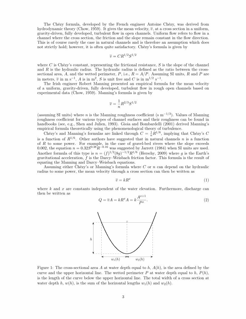
In this subsection we go through the formulas of Manning and Chézy for mean velocity inopen channels (Chow, 1959) and show how they depend on the cross-sectional area, A, and thewetted perimeter, P , defined as the circumference of the cross section excluding the free surface,see Figure 1. Note that both A and P depend on stage, h. By multiplying these formulaswith the cross-sectional area, formulas for discharge are obtained. These discharge formulas arethe product of physical constants and a geometry factor that changes with stage. In practice,estimation of discharge rating curves for open channels in nature is based on paired observationsof discharge and stage, but not on observations of cross-sectional area and wetted perimetersince these are usually not collected. Thus, estimation of discharge rating curves cannot bebased directly on the formulas of Manning and Chézy, and rating curves based on stage only,such as the generalized power-law rating curve, are needed. However, to understand how theproperties of the proposed generalized power-law rating curve relate to the physics of flow inopen channels, it is essential to have the general form of the physical discharge formulas sincethey include the physical parameters and the geometry.
Open channel flow has a free surface subject to atmospheric pressure as opposed to closedconduit flow, for example a pipe flow, where the flow is pressurized. The velocity of the flow isnot uniform over a given cross section; however, the mean velocity through the cross section is ofinterest in practice as it can be used to compute the discharge through a cross section, given thecross-sectional area. The discharge, and therefore the mean velocity, is governed by the balancebetween the gravitational force and a force due to frictional resistance (Chow, 1959).
2
The Chézy formula, developed by the French engineer Antoine Chézy, was derived fromhydrodynamic theory (Chow, 1959). It gives the mean velocity, v, at a cross section in a uniform,gravity-driven, fully developed, turbulent flow in open channels. Uniform flow refers to flow in achannel where the cross section, the friction and the slope remain constant in the flow direction.This is of course rarely the case in natural channels and is therefore an assumption which doesnot strictly hold; however, it is often quite satisfactory. Chézy’s formula is given by
v = CR1/2S1/2
where C is Chézy’s constant, representing the frictional resistance, S is the slope of the channeland R is the hydraulic radius. The hydraulic radius is defined as the ratio between the cross-sectional area, A, and the wetted perimeter, P , i.e., R = A/P . Assuming SI units, R and P arein meters, v in m s−1, A is in m2, S is unit free and C is in m1/2 s−1.
The Irish engineer Robert Manning presented an empirical formula for the mean velocityof a uniform, gravity-driven, fully developed, turbulent flow in rough open channels based onexperimental data (Chow, 1959). Manning’s formula is given by
v =1
nR2/3S1/2
(assuming SI units) where n is the Manning roughness coefficient (s m−1/3). Values of Manningroughness coefficient for various types of channel surfaces and their roughness can be found inhandbooks (see, e.g., Shen and Julien, 1993). Gioia and Bombardelli (2001) derived Manning’sempirical formula theoretically using the phenomenological theory of turbulence.
Chézy’s and Manning’s formulas are linked through C = 1nR
1/6, implying that Chézy’s Cis a function of R1/6. Other authors have suggested that in natural channels n is a functionof R to some power. For example, in the case of gravel-bed rivers where the slope exceeds0.002, the equation n = 0.32S0.38R−0.16 was suggested by Jarrett (1984) when SI units are used.Another formula of this type is n = (f)1/2(8g)−1/2R1/6 (Herschy, 2009) where g is the Earth’sgravitational acceleration, f is the Darcy–Weisbach friction factor. This formula is the result ofequating the Manning and Darcy–Weisbach equations.
Assuming either Chézy’s or Manning’s formula where C or n can depend on the hydraulicradius to some power, the mean velocity through a cross section can then be written as
v = kRx (1)
where k and x are constants independent of the water elevation. Furthermore, discharge canthen be written as
Q = vA = kRxA = kAx+1
P x. (2)
h
w2(h)w1(h)
Figure 1: The cross-sectional area A at water depth equal to h, A(h), is the area defined by thecurve and the upper horizontal line. The wetted perimeter P at water depth equal to h, P (h),is the length of the curve below the upper horizontal line. The total width of a cross section atwater depth h, w(h), is the sum of the horizontal lengths w1(h) and w2(h).
3
Note that in this form, neither formula is assumed over the other nor is it assumed that Chézy’sC or Manning’s n depend on some power of R; rather (1) is a generalized form of Chézy’s andManning’s formulas that takes into account the possibility that C or n may be functions of Rto some power. Chézy’s and Manning’s formulas with constant C and n are special cases of (1);while assuming C and n are a function of R to some power, the two formulas then coincide in(1). This formula is similar to what has been called the generalized friction law, v = K1R
xS1/2
(Petersen-Øverleir, 2006). Chow (1959) also noted that most uniform-flow formulas are of thegeneral form v = K2R
xSy. In the equations above K1 and K2 are constants independent of thewater elevation.
Table 3 in Appendix A contains a list of the hydrodynamic quantities and parameters foundin this subsection along with their units.
2.2 Generalization of the power-law rating curve
In this subsection we formally propose the generalized power-law rating curve. It is a general-ization of the power-law rating curve of the form
Q(h) = a(h− c)f(h), (3)
where a and c are constants and f(h) is the power-law exponent. The motivation for the form ofthe generalized power-law rating curve in (3) is given below, and it is demonstrated how physicsof open channels flow as presented by (2) enter into (3), i.e., what is the physical interpretationof a and how does the geometry in (2) affect f(h).
Although the power-law formula is empirical, it stems from theory. In particular, in the caseof a v-shaped cross section, both the Chézy formula and the Manning formula yield a power-lawrating curve with b = 2+x. For other shapes, there is no direct link between the power-law ratingcurve and the formulas of Chézy and Manning. The fact that the power-law formula is exact foruniform flow in the case of a v-shaped cross section indicates that an extension of the power-lawform might be a sensible form for rating curves in general. The logarithmic transformation ofthe power-law form gives a form that is linear in terms of the parameters log(a) and b, that is,logQ(h) = log(a) + b log(h− c), which is convenient for statistical inference. This model can beextended by allowing either one of log(a) and b to vary with h, or both of them. By modelinglog(a) and b as a function of h with a linear statistical model of some sort, the statistical inferencewill be easier for that model compared to a model that assumes nonlinear forms for log(a) andb. It is shown below that by allowing only b to vary with water elevation, a flexible form of arating curve can be developed which captures the physical nature of discharge in open channels.
To incorporate the physics of open channel flow into the generalized power-law rating curvein (3), the general formula for discharge in uniform flow given in (2) and the rating curve in (3)are equated with c = 0 for simplicity. Thus, in this subsection and in Section 2.3, h will representthe water depth. So, without any loss of generality,
Q(h) = ahf(h) = kA(h)x+1
P (h)x.
Solving for the power-law exponent f(h) and a gives Result 1 below. Here A(h) and P (h) denotethe cross-sectional area and the wetted perimeter, respectively, as a function of water depth h,and they are defined as
A(h) =
∫ h
0w1(η)dη +
∫ h
0w2(η)dη,
P (h) =
∫ h
0
√1 + {w′1(η)}2dη +
∫ h
0
√1 + {w′2(η)}2dη (4)
where w1(h) and w2(h) are two lengths that together that make up the width of the cross sectionat water depth h, see Figure 1. The terms w′1(h) and w′2(h) are the first derivatives of w1(h)and w2(h) with respect to h. It is assumed that w1(h) and w2(h) are continuous, and that w′1(h)and w′2(h) are piecewise continuous to ensure that the integrals for A(h) and P (h) exist and arecontinuous. Furthermore, it is assumed that the cross section is such that it forms a single areafor all values of the water depth, i.e., there cannot be two or more disjoint areas for any value
4

of the water depth. This means that w1(h) and w2(h) are always positive and can only take onevalue for each water depth h.
Result 1 The power-law exponent f(h) in (3) is given by
f(h) =
(x+ 1) log
{A(h)
A(1)
}− x log
{P (h)
P (1)
}
log(h)(5)
for h > 0 and h 6= 1. The constant a in (3) is given by
a = kA(1)x+1
P (1)x= Q(1).
A proof of Result 1 is given in Appendix B.1. Assuming that the model in (2) gives anaccurate description of discharge in a uniform gravity driven fully developed turbulent flow inopen channels with constant friction and constant slope in the flow direction, the model in (3)is simply another way to rewrite the model in (2) given that w1(h) and w2(h) are restricted tobeing positive and taking only one value for each water depth h. So, under these constrictions,the model in (3) is as flexible as the model in (2). That means the model given by (3) can beused to model any regular or irregular geometry in the cross section of open channels that fallsunder the constrictions.
Note that f(h) is affected by the geometry of the cross section and x but not by the parameterk. Since k is a function of the friction (C or n) and the slope (S), f(h) is not affected by thefriction nor the slope. The constant a is equal to Q(1), i.e., discharge when the depth is equalto 1 m, and that gives the simplest interpre
The proposed model in (3) can be used as a basis for a statistical model of the form
log(Qi) = log(a) + f(hi) log(hi − c) + εi (6)
where (hi, Qi) are the i-th water elevation/discharge observation and εi is the correspondingerror term. There are several ways to specify a model for f(h) within this statistical model. Theassumptions given for the model in (3) which involve wk(h) being continuous and w′k(h) beingpiecewise continuous, k = 1, 2, can be used as a reference. These assumptions lead to f(h) beingcontinuous and f ′(h) being piecewise continuous, since f(h) is a function of P (h) and A(h) andthe first derivative of P (h) is a function of the first derivative of wk(h), k = 1, 2, while the firstderivative of A(h) is a function of wk(h), k = 1, 2. So a finite number of jumps in f ′(h) could beallowed in a given interval over h. Statistical models with more restrictive constraints on f(h)than above may be more feasible for statistical inference, for example; (i) f(h) and f ′(h) arecontinuous; (ii) f(h), f ′(h) and f ′′(h) are continuous. As previously noted, a linear statisticalmodel for f(h) is desired, so, models that are linear in the statistical parameters, and fulfil oneof the three restrictions presented above, are candidates for f(h) in the statistical model givenby (6).
2.3 Properties of the generalized power-law rating curve
In this subsection the properties of the generalized power-law rating curve are explored throughthe power-law exponent f(h). Important properties of the power-law exponent f(h) are its limitsas h approaches zero from above, one and infinity. These limits are given in Result 2.
Result 2 Assume that w′′1(h) and w′′2(h) are continuous. The values of f(h) at h = 0 and h = 1are defined as the limit of f(h) as h approaches 0 from above and as h approaches 1, respectively.That is,
f(0) = limh→0+
f(h) = 1 + (x+ 1) limh→0+
hA′′(h)
A′(h)− x lim
h→0+
hP ′′(h)
P ′(h)(7)
andf(1) = lim
h→1f(h) = (x+ 1)
A′(1)
A(1)− xP
′(1)
P (1), (8)
5
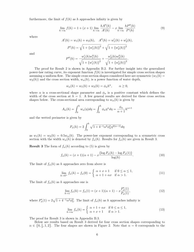
furthermore, the limit of f(h) as h approaches infinity is given by
limh→∞
f(h) = 1 + (x+ 1) limh→∞
hA′′(h)
A′(h)− x lim
h→∞hP ′′(h)
P ′(h)(9)
whereA′(h) = w1(h) + w2(h), A′′(h) = w′1(h) + w′2(h),
P ′(h) =
√1 + {w′1(h)}2 +
√1 + {w′2(h)}2
andP ′′(h) =
w′1(h)w′′1(h)√1 + {w′1(h)}2
+w′2(h)w′′2(h)√1 + {w′2(h)}2
.
The proof for Result 2 is shown in Appendix B.2. For further insight into the generalizedpower-law rating curve, its exponent function f(h) is investigated for simple cross section shapesassuming a uniform flow. The simple cross section shapes considered here are symmetric (w1(h) =w2(h)) and the cross section width, wα(h), is a power function of water depth,
wα(h) = w1(h) + w2(h) = φαhα, α ≥ 0,
where α is a cross-sectional shape parameter and φα is a positive constant which defines thewidth of the cross section at h = 1. A few general results are derived for these cross sectionshapes below. The cross-sectional area corresponding to wα(h) is given by
Aα(h) =
∫ h
0wα(η)dη =
∫ h
0φαη
αdη =φαα+ 1
hα+1
and the wetted perimeter is given by
Pα(h) = 2
∫ h
0
√1 + 4−1α2φ2αη
2(α−1)dη
as w1(h) = w2(h) = 0.5wα(h). The power-law exponent corresponding to a symmetric crosssection with the width wα(h) is denoted by fα(h). Results for fα(h) are given in Result 3.
Result 3 The form of fα(h) according to (5) is given by
fα(h) = (x+ 1)(α+ 1)− x{logPα(h)− logPα(1)}log(h)
. (10)
The limit of fα(h) as h approaches zero from above is
limh→0+
fα(h) = fα(0) =
{α+ x+ 1 if 0 ≤ α ≤ 1,α+ 1 + αx if α > 1.
(11)
The limit of fα(h) as h approaches one is
limh→1
fα(h) = fα(1) = (x+ 1)(α+ 1)− xP′α(1)
Pα(1), (12)
where P ′α(1) = 2√
1 + 4−1α2φ2α. The limit of fα(h) as h approaches infinity is
limh→∞
fα(h) =
{α+ 1 + αx if 0 ≤ α ≤ 1,α+ x+ 1 if α > 1.
(13)
The proof for Result 3 is shown in Appendix B.3.Below are results based on Result 3 derived for four cross section shapes corresponding to
α ∈{
0, 12 , 1, 2}. The four shapes are shown in Figure 2. Note that α = 0 corresponds to the
6
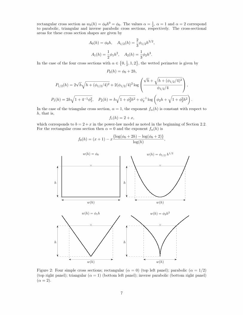
rectangular cross section as w0(h) = φ0h0 = φ0. The values α = 1
2 , α = 1 and α = 2 correspondto parabolic, triangular and inverse parabolic cross sections, respectively. The cross-sectionalareas for these cross section shapes are given by
A0(h) = φ0h, A1/2(h) =2
3φ1/2h
3/2,
A1(h) =1
2φ1h
2, A2(h) =1
3φ2h
3.
In the case of the four cross sections with α ∈{
0, 12 , 1, 2}, the wetted perimeter is given by
P0(h) = φ0 + 2h,
P1/2(h) = 2√h√h+ (φ1/2/4)2 + 2(φ1/2/4)2 log
√h+
√h+ (φ1/2/4)2
φ1/2/4
,
P1(h) = 2h√
1 + 4−1φ21, P2(h) = h√
1 + φ22h2 + φ−12 log
(φ2h+
√1 + φ22h
2
).
In the case of the triangular cross section, α = 1, the exponent fα(h) is constant with respect toh, that is,
f1(h) = 2 + x,
which corresponds to b = 2 + x in the power-law model as noted in the beginning of Section 2.2.For the rectangular cross section then α = 0 and the exponent fα(h) is
f0(h) = (x+ 1)− x{log(φ0 + 2h)− log(φ0 + 2)}log(h)
,
h
w(h)
w(h) = φ0
h
w(h)
w(h) = φ1/2 h1/2
h
w(h)
w(h) = φ1h
h
w(h)
w(h) = φ2h2
Figure 2: Four simple cross sections; rectangular (α = 0) (top left panel); parabolic (α = 1/2)(top right panel); triangular (α = 1) (bottom left panel); inverse parabolic (bottom right panel)(α = 2).
7
and its limits as h approaches zero and infinity are (x+ 1) and 1, respectively, and the limit off0(h) at h = 1 is
f0(1) = (x+ 1)− 2x/(2 + φ0).
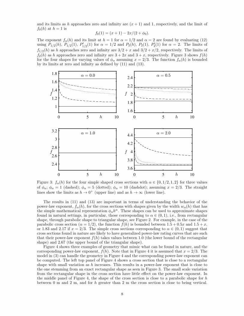
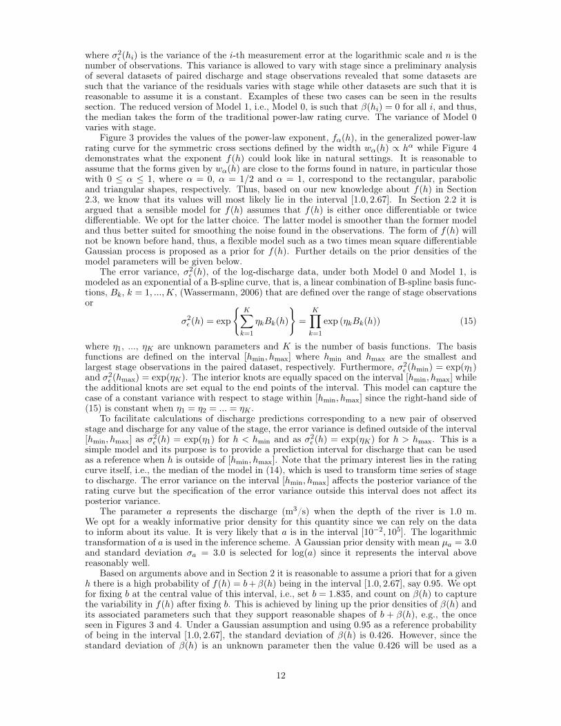
The exponent fα(h) and its limit at h = 1 for α = 1/2 and α = 2 are found by evaluating (12)using P1/2(h), P1/2(1), P ′1/2(1) for α = 1/2 and P2(h), P2(1), P ′2(1) for α = 2. The limits off1/2(h) as h approaches zero and infinity are 3/2 + x and 3/2 + x/2, respectively. The limits off2(h) as h approaches zero and infinity are 3 + 2x and 3 + x, respectively. Figure 3 shows f(h)for the four shapes for varying values of φα assuming x = 2/3. The function fα(h) is boundedby its limits at zero and infinity as defined by (11) and (13).
0 5 10
1
1.2
1.4
1.6
1.8
0 5 10
1.6
1.8
2
2.2
2.4
0 5 10
2.4
2.6
2.8
3
3.2
0 5 10
3.6
3.8
4
4.2
4.4
Figure 3: fα(h) for the four simple shaped cross sections with α ∈ {0, 1/2, 1, 2} for three valuesof φα; φα = 1 (dashed); φα = 5 (dotted); φα = 10 (dashdot); assuming x = 2/3. The straightlines show the limits as h→ 0+ (upper line) and as h→∞ (lower line).
The results in (11) and (13) are important in terms of understanding the behavior of thepower-law exponent, fα(h), for the cross sections with shapes given by the width wα(h) that hasthe simple mathematical representation φαhα. These shapes can be used to approximate shapesfound in natural settings, in particular, those corresponding to α ∈ (0, 1), i.e., from rectangularshape, through parabolic shape to triangular shape, see Figure 2. For example, in the case of theparabolic cross section (α = 1/2), the function f(h) is bounded between 1.5 + 0.5x and 1.5 + x,or 1.83 and 2.17 if x = 2/3. The simple cross sections corresponding to α ∈ (0, 1) suggest thatcross sections found in nature are likely to have generalized power-law rating curves that are suchthat their power-law exponent f(h) takes values between 1.0 (the lower bound of the rectangularshape) and 2.67 (the upper bound of the triangular shape).
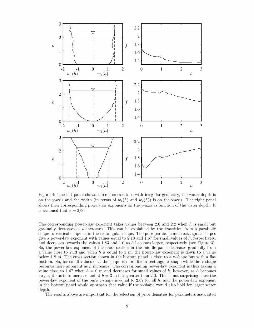
Figure 4 shows three examples of geometry that mimic what can be found in nature, and thecorresponding power-law exponent, f(h). Note that in Figure 4 it is assumed that x = 2/3. Themodel in (3) can handle the geometry in Figure 4 and the corresponding power-law exponent canbe computed. The left top panel of Figure 4 shows a cross section that is close to a rectangularshape with small variation as h increases. This results in a power-law exponent that is close tothe one stemming from an exact rectangular shape as seen in Figure 3. The small scale variationfrom the rectangular shape in the cross section have little effect on the power-law exponent. Inthe middle panel of Figure 4, the shape of the cross section is close to a parabolic shape for hbetween 0 m and 2 m, and for h greater than 2 m the cross section is close to being vertical.
8
-2 -1 0 1 2
0
1
2
3
0 1 2 3
1.4
1.6
1.8
2
2.2
-2 -1 0 1 2
0
1
2
3
0 1 2 3
1.4
1.6
1.8
2
2.2
-2 -1 0 1 2
0
1
2
3
0 1 2 3
1.4
1.6
1.8
2
2.2
Figure 4: The left panel shows three cross sections with irregular geometry, the water depth ison the y-axis and the width (in terms of w1(h) and w2(h)) is on the x-axis. The right panelshows their corresponding power-law exponents on the y-axis as function of the water depth. Itis assumed that x = 2/3.
The corresponding power-law exponent takes values between 2.0 and 2.2 when h is small butgradually decreases as h increases. This can be explained by the transition from a parabolicshape to vertical shape as in the rectangular shape. The pure parabolic and rectangular shapesgive a power-law exponent with values equal to 2.13 and 1.67 for small values of h, respectively,and decreases towards the values 1.83 and 1.0 as h becomes larger, respectively (see Figure 3).So, the power-law exponent of the cross section in the middle panel decreases gradually froma value close to 2.13 and when h is equal to 3 m, the power-law exponent is down to a valuebelow 1.8 m. The cross section shown in the bottom panel is close to a v-shape but with a flatbottom. So, for small values of h the shape is more like a rectangular shape while the v-shapebecomes more apparent as h increases. The corresponding power-law exponent is thus taking avalue close to 1.67 when h = 0 m and decreases for small values of h, however, as h becomeslarger, it starts to increase and at h = 3 m it is greater than 2.0. This is not surprising since thepower-law exponent of the pure v-shape is equal to 2.67 for all h, and the power-law exponentin the bottom panel would approach that value if the v-shape would also hold for larger waterdepth.
The results above are important for the selection of prior densities for parameters associated
9
with f(h) when modeling open channel flow in natural settings within a Bayesian statisticalframework, namely, whatever parameterization is used for f(h), it should be such that the se-lected prior densities of the parameters place f(h) in the interval [1.0, 2.67] with high probability.The model for f(h) and the prior densities of the parameters associated with f(h) will be intro-duced in Section 4.1.
3 Data
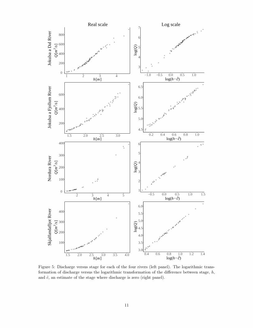
Four datasets were considered for a detailed analysis. They consist of paired observations ofdischarge and stage. Each dataset belongs to a specific observational site in Iceland. Thedata were collected by the Icelandic Meteorological Office (IMO) from rivers with quite diverseconditions at different locations in Iceland. The rivers are the Nordura River that runs throughthe Borgarfjordur region in central west Iceland (number of pairs n = 35); the SkjalfandafljotRiver, which has a source in the northwest of the Vatnajokull Icecap from where it flows northinto Skjalfandi Bay in central part of north Iceland (n = 56); the Jokulsa a Fjollum River locatedin the northeast of Iceland, its source being the Vatnajokull Icecap (n = 76); and the fourth riveris the Jokulsa a Dal River in eastern Iceland which now contains a reservoir for hydroelectricpower generation, with its source being the Bruarjokull Icecap (n = 86). The Nordura River isa spring water river with direct runoff components, and the other three rivers are glacial rivers.These rivers were the subject of a previous study described in Hrafnkelsson et al. (2012).
Figure 5 shows discharge versus stage in the left panel for the four rivers, and the right panelshows the logarithmic transformation of discharge versus the logarithmic transformation of thedifference between stage and c where c is an estimate of the stage where discharge is zero, i.e.,the posterior median of c under the power-law model. The plots in the right panel are such thatwhen the power-law rating curve is an adequate model then the data cluster around a straightline, and an estimate of its slope is an estimate of b in the power-law rating curve. The data fromthe Jokulsa a Fjollum River can be model adequately well with a straight line while that is notthe case for the data from the Jokulsa a Dal River. The data from the other two rivers appear todeviate from a straight line. Analysis of these four dataset in the Results section reveals whichof them can be described adequately well with the power-law rating curve and which require thegeneralized power-law rating curve.
4 Statistical modeling and inference
In this section we propose a statistical model based the generalized power-law rating curve alongwith an efficient Bayesian inference scheme for the model. This statistical model, referred to asModel 1, will be compared to a statistical model based on the power-law rating curve, referredto as Model 0.
4.1 Bayesian models for discharge rating curves
The proposed statistical model for discharge observation, Model 1, assumes that its median isgiven by the generalized power-law rating curve, that is ,
Q(h) = a(h− c)f(h),
where, as before, the power-law exponent f(h) is a function of stage, h, the parameter c is thestage at which the discharge is zero while the parameter a is a scaling parameter that can beinterpreted as the discharge when the corrected stage, h − c, is equal to 1.0 m. The power-lawexponent is parameterized as a sum of a constant b and deviations β(h), that is,
f(h) = b+ β(h).
The i-th discharge observation Qi, conditional on its corresponding stage, hi, is modeled as alognormal variable,
Qi ∼ LN(log(a) + {b+ β(hi)} log(hi − c), σ2ε (hi)), i = 1, ..., n, (14)
10
0
200
400
600
800
1 2 3 4h[m]
Q[m
3/s
]
Real scale
Joku
lsa
a D
al R
iver
3
4
5
6
7
−1.0 −0.5 0.0 0.5 1.0log(h−c)
log(
Q)
Log scale
200
400
600
1.5 2.0 2.5 3.0h[m]
Q[m
3/s
]
Joku
lsa
a F
jollu
m R
iver
4.5
5.0
5.5
6.0
6.5
0.2 0.4 0.6 0.8 1.0log(h−c)
log(
Q)
0
100
200
300
400
2 3 4 5h[m]
Q[m
3/s
]
Nor
dura
Riv
er
1
2
3
4
5
6
−0.5 0.0 0.5 1.0 1.5log(h−c)
log(
Q)
100
200
300
400
1.5 2.0 2.5 3.0 3.5 4.0h[m]
Q[m
3/s
]
Skj
alfa
ndaf
ljot R
iver
3.0
3.5
4.0
4.5
5.0
5.5
6.0
0.4 0.6 0.8 1.0 1.2 1.4log(h−c)
log(
Q)
Figure 5: Discharge versus stage for each of the four rivers (left panel). The logarithmic trans-formation of discharge versus the logarithmic transformation of the difference between stage, h,and c, an estimate of the stage where discharge is zero (right panel).
11
where σ2ε (hi) is the variance of the i-th measurement error at the logarithmic scale and n is thenumber of observations. This variance is allowed to vary with stage since a preliminary analysisof several datasets of paired discharge and stage observations revealed that some datasets aresuch that the variance of the residuals varies with stage while other datasets are such that it isreasonable to assume it is a constant. Examples of these two cases can be seen in the resultssection. The reduced version of Model 1, i.e., Model 0, is such that β(hi) = 0 for all i, and thus,the median takes the form of the traditional power-law rating curve. The variance of Model 0varies with stage.
Figure 3 provides the values of the power-law exponent, fα(h), in the generalized power-lawrating curve for the symmetric cross sections defined by the width wα(h) ∝ hα while Figure 4demonstrates what the exponent f(h) could look like in natural settings. It is reasonable toassume that the forms given by wα(h) are close to the forms found in nature, in particular thosewith 0 ≤ α ≤ 1, where α = 0, α = 1/2 and α = 1, correspond to the rectangular, parabolicand triangular shapes, respectively. Thus, based on our new knowledge about f(h) in Section2.3, we know that its values will most likely lie in the interval [1.0, 2.67]. In Section 2.2 it isargued that a sensible model for f(h) assumes that f(h) is either once differentiable or twicedifferentiable. We opt for the latter choice. The latter model is smoother than the former modeland thus better suited for smoothing the noise found in the observations. The form of f(h) willnot be known before hand, thus, a flexible model such as a two times mean square differentiableGaussian process is proposed as a prior for f(h). Further details on the prior densities of themodel parameters will be given below.
The error variance, σ2ε (h), of the log-discharge data, under both Model 0 and Model 1, ismodeled as an exponential of a B-spline curve, that is, a linear combination of B-spline basis func-tions, Bk, k = 1, ...,K, (Wassermann, 2006) that are defined over the range of stage observationsor
σ2ε (h) = exp
{K∑
k=1
ηkBk(h)
}=
K∏
k=1
exp (ηkBk(h)) (15)
where η1, ..., ηK are unknown parameters and K is the number of basis functions. The basisfunctions are defined on the interval [hmin, hmax] where hmin and hmax are the smallest andlargest stage observations in the paired dataset, respectively. Furthermore, σ2ε (hmin) = exp(η1)and σ2ε (hmax) = exp(ηK). The interior knots are equally spaced on the interval [hmin, hmax] whilethe additional knots are set equal to the end points of the interval. This model can capture thecase of a constant variance with respect to stage within [hmin, hmax] since the right-hand side of(15) is constant when η1 = η2 = ... = ηK .
To facilitate calculations of discharge predictions corresponding to a new pair of observedstage and discharge for any value of the stage, the error variance is defined outside of the interval[hmin, hmax] as σ2ε (h) = exp(η1) for h < hmin and as σ2ε (h) = exp(ηK) for h > hmax. This is asimple model and its purpose is to provide a prediction interval for discharge that can be usedas a reference when h is outside of [hmin, hmax]. Note that the primary interest lies in the ratingcurve itself, i.e., the median of the model in (14), which is used to transform time series of stageto discharge. The error variance on the interval [hmin, hmax] affects the posterior variance of therating curve but the specification of the error variance outside this interval does not affect itsposterior variance.
The parameter a represents the discharge (m3/s) when the depth of the river is 1.0 m.We opt for a weakly informative prior density for this quantity since we can rely on the datato inform about its value. It is very likely that a is in the interval [10−2, 105]. The logarithmictransformation of a is used in the inference scheme. A Gaussian prior density with mean µa = 3.0and standard deviation σa = 3.0 is selected for log(a) since it represents the interval abovereasonably well.
Based on arguments above and in Section 2 it is reasonable to assume a priori that for a givenh there is a high probability of f(h) = b+β(h) being in the interval [1.0, 2.67], say 0.95. We optfor fixing b at the central value of this interval, i.e., set b = 1.835, and count on β(h) to capturethe variability in f(h) after fixing b. This is achieved by lining up the prior densities of β(h) andits associated parameters such that they support reasonable shapes of b + β(h), e.g., the onceseen in Figures 3 and 4. Under a Gaussian assumption and using 0.95 as a reference probabilityof being in the interval [1.0, 2.67], the standard deviation of β(h) is 0.426. However, since thestandard deviation of β(h) is an unknown parameter then the value 0.426 will be used as a
12
reference value, see below. Under the reduced model, Model 0, it is assumed that the functionβ(h) is zero, and under this model the parameter b is assigned a Gaussian prior density withmean 1.835 and standard deviation 0.426.
In accordance with our assumption of a twice differentiable f(h), we propose modeling thefunction β(h) with a mean zero Gaussian process that is governed by a Matérn covariancefunction with marginal standard deviation σβ , range parameter φβ and smoothness parameterν. The amplitude of the process is controlled by σβ , φβ governs how fast the spatial correlationof the process decays with increasing distance d and ν controls the smoothness of the process.In general, if 2 < ν ≤ 3 then the Matérn process is two times mean-square differentiable. Herethe value ν = 5/2 is selected as that correlation function has a relatively simple form. Theprior density of the vector β = (β1, ..., βn)T where βi = β(hi) is Gaussian with mean zero andcovariance matrix Σβ , i.e., β ∼ N(0,Σβ), where the (i, j)-th element of Σβ is
{Σβ}i,j = Cov(β(hi), β(hj)) = σ2β
(1 +
√5di,jφβ
+5di,j3φ2β
)exp
(−√
5di,jφβ
)(16)
where di,j = |hi − hj | is the distance between stages hi and hj . The prior densities for σβ andφβ are described below.
The parameter c is assigned a prior density that is such that the quantity hmin − c has anexponential density with rate parameter λ1 where hmin is either the smallest stage in the paireddataset (h1, Q1), ..., (hn, Qn) or the smallest stage found in other data sources for the river understudy. Thus, the prior density for c is set after seeing data on stage only while the posteriordensity of c is determined based on the paired dataset. Here, after exploring other datasets fromIceland, λ1 is selected such that the probability of hmin − c being greater than 1.5 m is 0.05which corresponds to λ1 = 2. In the case of datasets from other areas, the value of λ1 should bereconsidered. The parameter c is transformed to ψ1 = log(hmin − c). The prior density for ψ1 is
π(ψ1) = λ1 exp(−λ1 exp(ψ1) + ψ1), ψ1 ∈ R.
The prior density for (σβ, φβ) is based on the Penalised Complexity (PC) prior density forthe Matérn parameters derived in Fuglstad et al. (2019). The PC approach for the selection ofprior densities is based on setting up a base model, i.e., a simpler model that is reasonable toshrink towards (Simpson et al., 2017). Here, in the case of β(h) and its parameters, using thePC prior density of Fuglstad et al. (2019), means that the base model is the one with the rangeequal to infinity and the marginal standard deviation equal to zero. So, if the data suggest thatβ(h) is constant in the observed interval of stages then the PC prior density supports that, i.e., itsupports that one over the range takes values arbitrary close to zero. Or, if the data suggest thatthe marginal standard deviation is zero or relatively small then the PC prior density supportsthese scenarios as well. Thus, the joint prior density of (β, σβ, φβ) allows realizations of β thatare close to being constant or smoothly varying in the observed interval of stages, and such thatf(h) is most likely in the interval [1.0, 2.67]
The form of the prior density for (σβ, φβ) is given by
π(σβ, φβ) = λ2 exp(−λ2σβ)λ3(2φβ)−3/2 exp(−λ3(2φβ)−1/2),
where the parameter ρ in Fuglstad et al. (2019) is such that ρ = 2φβ . The values of the parametersλ2 and λ3 are found by specifying the reference value σβ,0 for σβ , and the reference value φβ,0for φβ , and assuming that the probability of σβ being above σβ,0 is α2, and that the probabilityof φβ being below φβ,0 is α3. Here the following values are selected
σβ,0 = 0.426, α2 = 0.10, φβ,0 = 1.5, α3 = 0.10,
where φβ,0 is in meters. Selecting σβ,0 = 0.426 is related to the arguments above, namely,conditional on σβ = 0.426, the probability of b + β(h) being outside the interval [1.0, 2.67] is0.05. If σβ is greater than 0.426 then this probability increases, so, setting α2 equal to 0.10equates putting small prior probability on that scenario.
Furthermore, having the range parameter above 1.5 m with prior probability 0.90 ensuresslow changes in β(h) within a relatively short interval, e.g., of length 0.5 m. Then λ2 and λ3 are
λ2 = − log(α2)(σβ,0)−1 = 5.405, λ3 = − log(α1)(2φβ,0)
1/2 = 3.988.
13
The parameters σβ and φβ are transformed to ψ2 = log(σβ) and ψ3 = log(φβ). The prior densityfor (ψ2, ψ3) is
π(ψ2, ψ3) = λ2 exp(−λ2 exp(ψ2) + ψ2)λ32−3/2 exp(−1.5ψ3) exp(−λ3(2)−1/2 exp(−0.5ψ3) + ψ3),
where ψ2, ψ3 ∈ R. Since π(ψ2, ψ3) factorizes it can written as π(ψ2, ψ3) = π(ψ2)π(ψ3).The parameter η1 is directly linked to the standard deviation of the error term when h = hmin
through σε(hmin) = exp(0.5η1), hmin being the smallest stage in the paired data . Simpson et al.(2017) found that the PC prior density for the standard deviation in a Gaussian density, whenthe base model has a standard deviation equal to zero, is an exponential density. We believea priori that σε(hmin) can be arbitrary close to zero, thus, this PC prior density is appropriatefor this parameter. Furthermore, by exploring other datasets, we find it reasonable to set theprior density for σε(hmin) such that it is likely to be below the value 0.08. Thus, we calibratethe exponential prior density for σε(hmin) such that the probability of exceeding the value 0.08is 0.10, giving the rate is λ5 = 28.78. This is equivalent of η1 having the prior density
π(η1) =1
2λ5 exp (−λ5 exp(0.5η1) + 0.5η1) , η1 ∈ R.
The prior density of η−1 = (η2, ..., ηK), conditional on η1 and the standard deviation parameterση, is specified in terms of Gaussian densities, that is,
π(η−1|η1, ση) =K∏
k=2
N(ηk|ηk−1, σ2η),
which is a random walk prior. This prior density of η−1 can be presented as
π(η−1|η1, ση) = (2πσ2η)−(K−1)/2 exp
(− 1
2σ2ηηTRηη
),
where η = (η1, ..., ηK). The prior density of η, conditional on ση, is π(η|ση) = π(η1)π(η−1|η1, ση).Here K is set equal to 6. In the case of K = 6 then
Rη =
1 −1 0 0 0 0−1 2 −1 0 0 00 −1 2 −1 0 00 0 −1 2 −1 00 0 0 −1 2 −10 0 0 0 −1 1
,
see Rue and Held (2005, Section 3.3.1, p. 95).Again, motivated by the PC approach of Simpson et al. (2017) for the selection of prior
densities, we assign an exponential prior density to the standard deviation parameter ση. Thisis in line with our modeling approach as we believe that the standard deviation σε(h) can bea constant in some cases and that corresponds to ση being equal to zero. This prior density isselected such that the probability of ση exceeding the value 0.267 is 0.10 which corresponds toa rate parameter λ4 = 8.62. This is motivated by the fact that when the value of ση is 0.267then for K = 6 the value of exp(0.5ηK), i.e., the standard deviation at h = hmax (hmax beingthe largest stage in the paired data), can become more than two times larger than exp(0.5η1),with probability 0.01 and it can become less than half of the size of exp(0.5η1) with probability0.01. The parameter ση is transformed to ψ4 = log(ση). The prior density for ψ4 is
π(ψ4) = λ4 exp(−λ4 exp(ψ4) + ψ4), ψ4 ∈ R.
With the aim of improving the sampling scheme for the posterior density presented in Sec-tion 4.2, the parameters η2, ..., ηK are transformed to z2, ..., zK , where ηk = η1+
∑km=2 σηzm, k =
2, ...,K. The conditional prior density of the z parameters is π(z2, ..., zK |η1, ση) =∏Kk=2N(zk|0, 1) =∏K
k=2 π(zk), i.e., that of independent Gaussian variates with mean zero and variance one.
14
Let ψ5 = η1, and ψk+4 = zk, k = 2, ...,K. Then the prior density of ψ = (ψ1, ..., ψK+4) is
π(ψ) =K+4∏
k=1
π(ψk).
The parameters inψ are the hyperparameters of Model 1 and its latent parameters are (log(a), b,β),but recall that b is set equal to 1.835. The latent parameters of Model 0 are (log(a), b) and itshyperparameters are (ψ1, ψ4, ..., ψK+4).
4.2 Posterior sampling scheme
We propose a Markov chain Monte Carlo (MCMC) sampling scheme that is based on proposingthe hyperparameters and the latent parameters jointly to sample from the posterior density.Our sampling scheme is motivated by the work of Knorr-Held and Rue (2002). The posteriordensities of Model 0 and Model 1 can be presented as
π(x,ψ|y) ∝ π(y|x,ψ)π(x|ψ)π(ψ)
where y = (Q1, ..., Qn)T contains the discharge observations, and x and ψ denote the latentparameters and the hyperparameters, respectively, of either Model 0 or Model 1. The data densityπ(y|x,ψ) is the product of lognormal densities with location and scale parameters describedby (14) and (15), respectively, while π(x|ψ) denotes the Gaussian prior density of the latentparameters under either Model 0 or Model 1 conditional on the hyperparameters.
Under Model 1 let A = (1 g G) where 1 is a vector of ones, g and G are a vector and adiagonal matrix, respectively, such that gi = Gii = log(hi − c), i = 1, ..., n. The prior mean andcovariance of x are µx = (3.0, 1.835,0T)T and Σx = bdiag(3.02, 0,Σβ), respectively, where bdiagdenotes a block diagonal matrix and 0 is a vector of zeros. Under Model 0 then A = (1 g),and the prior mean and covariance of x are µx = (3.0, 1.835)T and Σx = diag(3.02, 0.4262),respectively. The diagonal matrix Σε is such that its i-th diagonal element is σ2ε (hi) and it isthe same under Models 0 and 1. The location and scale parameters of π(y|x,ψ) are Ax and Σε,respectively.
The proposed MCMC sampling scheme is as follows. The k-th posterior sample of (x,ψ) isobtained by
sampling ψ(k) from π(ψ|y) ∝ π(ψ)π(y|ψ)
sampling x(k) from π(x|y,ψ(k))
and ψ(k) and x(k) are accepted jointly, so, if ψ(k) is rejected, sampling of x(k) can be delayed.This is due to the fact that the acceptance ratio for a proposal (ψ∗,x∗) is independent of x(k−1)
and x∗ (see Knorr-Held and Rue, 2002; Geirsson et al., 2020). The conditional posterior densityπ(x|y,ψ(k)) is a multivariate Gaussian density derived from π(y|x,ψ)π(x|ψ). It has mean
µx|y = µx − ΣxAT(AΣxA
T + Σε)−1(Aµx − v)
where v = (log(Q1), ..., log(Qn)) and covariance
Σx|y = Σx − ΣxAT(AΣxA
T + Σε)−1AΣx.
This is essentially the one block sampler of Knorr-Held and Rue (2002) in the case where thedata density is lognormal. The marginal posterior density π(ψ|y) is known up to a normalizingconstant. The marginal density of y, π(y|ψ), is lognormal with location and scale parametersAµx and AΣxA
T + Σε, respectively. It is found by deriving the marginal distribution of y(conditional on ψ) from the joint density of (y,x), i.e., π(y|x,ψ)π(x|ψ).
To obtain draws of ψ, a random-walk Metropolis algorithm was used with a proposal density,q(·|·), that is a multivariate Gaussian density centered on the last draw and with precision matrixu−1(−H), where H is a finite difference estimate of the Hessian matrix of log(π(ψ|y)) evaluated
15
at the mode of log(π(ψ|y)) with the mode denoted by ψ, also referred to as the posterior modeof ψ. H is given by
H ' ∇2 log(π(ψ|y))∣∣ψ=ψ
and u is a scaling constant given by u = 2.382/dim(ψ), see Roberts et al. (1997).Roberts et al. (1997) show that this scaling is optimal in a particular large dimension scenario.
It turns out that this scaling works well for Model 0 and Model 1. Setting a specific scaling thatis efficient removes the need for tuning. The proposal value ψ in the k-th iteration given thedraw of the (k − 1)-th iteration, ψ(k−1), is thus drawn from the following Gaussian density,
π(ψ|ψ(k−1)) = N(ψ|ψ(k−1), u(−H)−1).
4.3 Prediction of discharge at observed and unobserved stage
To sample from the posterior predictive distribution of discharge Qi under Model 1 with stagehi found in the paired dataset then we sample first x(l) and ψ(l) from the posterior density andthen we draw a sample from
Qi ∼ LN(log(a)(l) + {b+ β(hi)(l)} log(hi − c(l)), σ2ε (hi)(l)).
To draw a sample from the posterior predictive distribution of discharge Qun correspondingunobserved stage hun under Model 1, we use
Qun ∼ LN(log(a)(l) + {b+ β(hun)(l)} log(hun − c(l)), σ2ε (hun)(l)),
and β(hun)(l) is drawn from the conditional Gaussian density
π(β(hun)|β(l), ψ(l)2 , ψ
(l)3 ) = N(β(hun)|γTΣ−1β β
(l), σ2β − γTΣβγ),
where γ = cov(β, β(hun)) is the covariance between β(hun) and the elements of β, found fromthe Matérn covariance function in (16), and γ, Σβ and σ2β are evaluated with ψ2 = ψ
(l)2 and
ψ3 = ψ(l)3 . Samples from the posterior predictive distribution of discharge Q0 for observed or
unobserved stage h0 under Model 0 can be drawn from
Q0 ∼ LN(log(a)(l) + b(l) log(h0 − c(l)), σ2ε (h0)(l)),where the values of the parameters are equal to the l-th draw from the posterior distribution of(x,ψ) under Model 0.
5 Results
Here results based on a detailed analysis of the data from the four rivers introduced in Section 3are given. This analysis was based on applying the two statistical models introduced in Section4.1 to the data and comparing these two models.
5.1 Computation and Convergence Assessment
Four chains were simulated for Model 0 and Model 1 where each chain consisted of 18,000iterations and 2,000 burn-in iterations. This proved sufficient for all datasets. For both models athinning factor of 5 was used, meaning every 5-th sample is kept for statistical inference and therest discarded. Running the four chains in parallel with code written in Matlab on an Intel(R)Core(TM) i5-7300U CPU (2.7GHz clock speed, 4 cores) with 16GB RAM simulations took 27seconds for Model 0 and 65 seconds for Model 1 for the largest dataset (86 observations).
Convergence in simulations from the posterior was ensured by assessing the Gelman-Rubinstatistic (Gelman and Rubin, 1992; Gelman et al., 2013), an estimate of a potential scale reductionfactor, and by visually assessing trace plots, histograms and the autocorrelation function for agiven simulated parameter (see the Supplementary Material). The proposed posterior samplingschemes worked well judging from the Gelman–Rubin statistics, the autocorrelation functionplots and visual inspection of the trace plots. The autocorrelation between samples 50 iterationsapart (no thinning applied) was at most 0.2 and the Gelman–Rubin statistic was safely underreference bounds when the length of the chains after burn-in was greater than 10000.
16

5.2 Estimates of parameters and functions
The two statistical models proposed in Section 4.1 were applied to the datasets from the fourrivers. Table 1 presents posterior summary statistics of selected parameter of these two modelsfor the four rivers. The estimates of the parameters a and c are somewhat different between thetwo models and the uncertainty in a and c in Model 1 is larger than in Model 0. The parameterb in Model 0 is presented along with b+ β(2) in Model 1 (the power-law exponent at h = 2 m)to provide comparison of the exponents of the two models. In the case of the Jokulsa a FjollumRiver the 95% posterior intervals of these two quantities overlap the most and their widths aresimilar while for the other three rivers the 95% posterior intervals for b + β(2) in Model 1 arewider by a factor 1.7 to 3.1 than those for for b in Model 0.
Table 1: The 2.5%, 50% and 97.5% posterior percentiles of the parameters a (m3/s), b and c (m)in Model 0 and the parameters a (m3/s), b+ β(2) and c (m) in Model 1.
Model 0 Model 1
River Param. 2.5% 50% 97.5% Param. 2.5% 50% 97.5%
Jokulsa a Dal a 84.68 101.85 118.73 a 34.61 73.87 99.96b 1.71 1.85 2.01 b+ β(2) 1.91 2.20 2.85c 0.61 0.70 0.78 c 0.28 0.57 0.72
Jokulsa a Fjollum a 44.58 73.98 107.70 a 52.91 94.38 119.52b 1.84 2.09 2.40 b+ β(2) 1.75 1.93 2.31c 0.06 0.32 0.52 c 0.15 0.44 0.58
Nordura a 12.59 15.82 19.11 a 14.30 19.42 22.82b 1.97 2.15 2.31 b+ β(2) 1.63 1.85 2.22c 0.80 0.89 0.97 c 0.83 0.98 1.07
Skjalfandafljot a 3.80 6.38 10.03 a 6.21 25.25 47.89b 2.85 3.11 3.39 b+ β(2) 1.61 2.06 2.96c -0.20 0.00 0.17 c -0.08 0.55 0.91
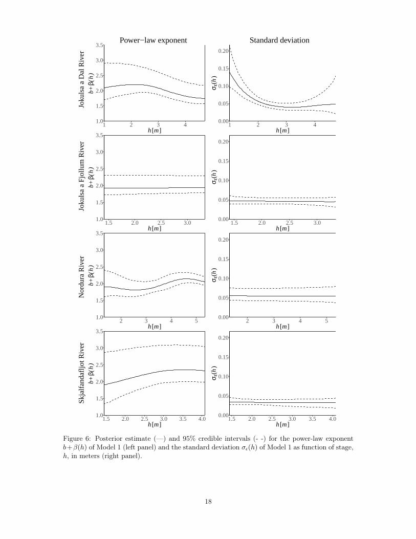
Figure 6 displays the power-law exponent b+β(h) and the standard deviation σε(h) of Model1 as a function of stage. The power-law exponent, b + β(h), of the Jokulsa a Fjollum River isclose to being constant with respect to stage according to the posterior estimate, while it showssome variation with stage in the case of the other rivers. The power-law exponent can reveal thegeometry of the cross section of the corresponding river at the observational site. For example,in the case of the Jokulsa a Dal River, the posterior estimate of the process b+β(h) takes valuesslightly above 2.0 for low stage and for greater values of stage it takes values around 1.75, and issimilar to b+ β(h) of the simulated river in the middle panel of Figure 4, indicating a parabolic-like shape for low stage and vertical river walls for higher stage. The wide posterior intervals forb + β(h) in the case of the Nordura River for values of stage between h = 3.5 m and h = 4.5m stem from the fact that none of the paired observations take stage values in this interval butthey take stage values below and above the interval. The posterior estimates of the standarddeviation process σε(h) indicate that it varies with stage in the case of the Jokulsa a Dal Riverwhile it is effectively constant for the other three rivers.
The left panel of Figure 7 shows estimates of rating curves and predictive intervals for thefour rivers under Model 1. Note that stage is shown on the vertical axes and discharge onthe horizontal axes as this is the standard practice in hydrology. The generalized rating curvesprovided a convincing fit to the four datasets. Residual plots are presented in the right panel ofFigure 7 along with the prediction intervals and credible intervals for expected value of log(Q)on the same scale, but with the prediction estimates subtracted for better visualization. Theresidual plots indicate that the mean of Model 1 captures the underlying mean and that the
17
1.0
1.5
2.0
2.5
3.0
3.5
1 2 3 4h[m]
b+
β(h
)
Power−law exponent
Joku
lsa
a D
al R
iver
0.00
0.05
0.10
0.15
0.20
1 2 3 4h[m]
σ ε(h
)
Standard deviation
1.0
1.5
2.0
2.5
3.0
3.5
1.5 2.0 2.5 3.0h[m]
b+
β(h
)
Joku
lsa
a F
jollu
m R
iver
0.00
0.05
0.10
0.15
0.20
1.5 2.0 2.5 3.0h[m]
σ ε(h
)
1.0
1.5
2.0
2.5
3.0
3.5
2 3 4 5h[m]
b+
β(h
)
Nor
dura
Riv
er
0.00
0.05
0.10
0.15
0.20
2 3 4 5h[m]
σ ε(h
)
1.0
1.5
2.0
2.5
3.0
3.5
1.5 2.0 2.5 3.0 3.5 4.0h[m]
b+
β(h
)
Skj
alfa
ndaf
ljot R
iver
0.00
0.05
0.10
0.15
0.20
1.5 2.0 2.5 3.0 3.5 4.0h[m]
σ ε(h
)
Figure 6: Posterior estimate (—) and 95% credible intervals (- -) for the power-law exponentb+β(h) of Model 1 (left panel) and the standard deviation σε(h) of Model 1 as function of stage,h, in meters (right panel).
18

standard deviation of Model 1 describes the variability in the measurement errors as a functionof stage adequately well. The wide posterior predictive intervals in the case of the Nordura Riverin the range from h = 3.5 m to 4.5 m are due to the absence of observations in this range ofstage values.
5.3 Model comparison
Three statistics were used to compare Model 0 and Model 1. These three statistics are thedeviance information criterion (DIC), posterior model probabilities (based on Bayes factor) andthe average absolute prediction error in a leave-one-out cross-validation. These statistics aredescribed below.
DIC quantifies the fit of a model to data with respect to the complexity of the model (Spiegel-halter et al., 2002). It is given by
DIC = Davg + pD
where Davg measures the fit of the model to the data. It is estimated with
Davg = − 2
L
L∑
l=1
log π(y|ξ(l))
where π(y|ξ(l)) is the likelihood function which arises from the proposed probability model ofthe data and ξ(l) = (x(l),ψ(l)) is the l-th posterior sample of the parameters of the model.Lower values of Davg indicate a better fit to the data. pD measures the complexity of themodel and is referred to as the effective number of parameters. It is usually less then the actualnumber of parameters, but these two numbers can be equal in some cases. pD is computedwith pD = Davg −Dψ where Dψ is another measure of fit that is given by −2 log π(y|ξ), here ξcontains the posterior median of each parameter. DIC presents a trade-off between the fit of amodel to the data and the model’s complexity, and it allows for comparison between models ofdifferent complexity in terms of the same dataset.
The posterior probabilities of Model 0 and Model 1 were computed using the Bayes factor andassuming a priori that the two models were equally likely (see Jeffreys, 1961; Kass and Raftery,1995). The posterior probability of Model 1 when comparing it to Model 0 is given by
P(M1|y) =P(M1)
∫H1π1(y|ξ1)π(ξ1)dξ1∑
s=0,1 P(Ms)∫Hsπs(y|ξs)π(ξs)dξs
=
(1 +
P(M0)
P(M1)× 1
B10
)−1
where B10 is the Bayes factor for the comparison of models M1 and M0 (see Kass and Raftery,1995). B10 is given by
B10 =
∫H1π1(y|ξ1)π(ξ1)dξ1∫
H0π0(y|ξ0)π(ξ0)dξ0
and here it is computed by approximating the integrals∫Hsπs(y|ξs)π(ξs)dξs, s = 0, 1, with the
harmonic mean of the likelihood values, i.e.,{
1
L
L∑
l=1
1
πs(y|ξ(l)s )
}−1
where ξ(l)s is the l-th posterior sample of ξs in Model s, see Newton and Raftery (1994) fordetails. However, in some cases the theoretical variance of the harmonic mean estimator is notfinite (Newton and Raftery, 1994), and even when it is finite, it can become very large since asmall fraction of the posterior samples can correspond to a small likelihood which will have alarge effect on the harmonic mean estimate. Furthermore, the harmonic mean estimator can bebiased even though it is asymptotically unbiased (Raftery et al., 2007; Calderhead and Girolami,
19
2009). Thus, here, the posterior model probabilities are treated with caution and viewed inlight of the other model comparison statistics. Additionally, a simulation study is provided inAppendix C to assess the variability in the estimated posterior model probabilities and in thedifference in DIC values.
A leave-one-out cross-validation was applied to both Model 0 and Model 1. For each datasetand Model s, one of the observations was left out and then the expected value of log(Q) waspredicted for that stage using an Empirical Bayes type approximation to save computation, i.e.,the posterior mode of the hyperparameters was used but their uncertainty was not taken intoaccount. The absolute value of the difference between the logarithm of the observed dischargeand the prediction was computed. This was done for all of the observations within the dataset.Finally, the average of these absolute differences, ADcv,i, was computed.
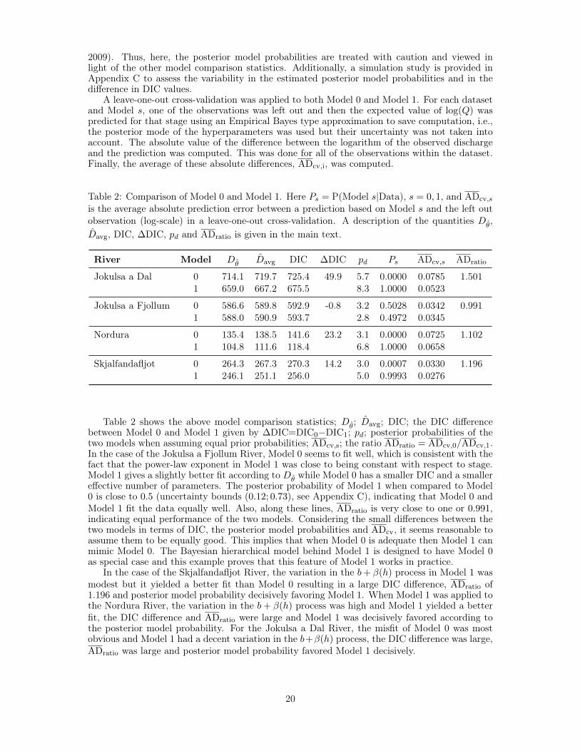
Table 2: Comparison of Model 0 and Model 1. Here Ps = P(Model s|Data), s = 0, 1, and ADcv,sis the average absolute prediction error between a prediction based on Model s and the left outobservation (log-scale) in a leave-one-out cross-validation. A description of the quantities Dθ,Davg, DIC, ∆DIC, pd and ADratio is given in the main text.
River Model Dθ Davg DIC ∆DIC pd Ps ADcv,s ADratio
Jokulsa a Dal 0 714.1 719.7 725.4 49.9 5.7 0.0000 0.0785 1.5011 659.0 667.2 675.5 8.3 1.0000 0.0523
Jokulsa a Fjollum 0 586.6 589.8 592.9 -0.8 3.2 0.5028 0.0342 0.9911 588.0 590.9 593.7 2.8 0.4972 0.0345
Nordura 0 135.4 138.5 141.6 23.2 3.1 0.0000 0.0725 1.1021 104.8 111.6 118.4 6.8 1.0000 0.0658
Skjalfandafljot 0 264.3 267.3 270.3 14.2 3.0 0.0007 0.0330 1.1961 246.1 251.1 256.0 5.0 0.9993 0.0276
Table 2 shows the above model comparison statistics; Dθ; Davg; DIC; the DIC differencebetween Model 0 and Model 1 given by ∆DIC=DIC0−DIC1; pd; posterior probabilities of thetwo models when assuming equal prior probabilities; ADcv,s; the ratio ADratio = ADcv,0/ADcv,1.In the case of the Jokulsa a Fjollum River, Model 0 seems to fit well, which is consistent with thefact that the power-law exponent in Model 1 was close to being constant with respect to stage.Model 1 gives a slightly better fit according to Dθ while Model 0 has a smaller DIC and a smallereffective number of parameters. The posterior probability of Model 1 when compared to Model0 is close to 0.5 (uncertainty bounds (0.12; 0.73), see Appendix C), indicating that Model 0 andModel 1 fit the data equally well. Also, along these lines, ADratio is very close to one or 0.991,indicating equal performance of the two models. Considering the small differences between thetwo models in terms of DIC, the posterior model probabilities and ADcv, it seems reasonable toassume them to be equally good. This implies that when Model 0 is adequate then Model 1 canmimic Model 0. The Bayesian hierarchical model behind Model 1 is designed to have Model 0as special case and this example proves that this feature of Model 1 works in practice.
In the case of the Skjalfandafljot River, the variation in the b+ β(h) process in Model 1 wasmodest but it yielded a better fit than Model 0 resulting in a large DIC difference, ADratio of1.196 and posterior model probability decisively favoring Model 1. When Model 1 was applied tothe Nordura River, the variation in the b+ β(h) process was high and Model 1 yielded a betterfit, the DIC difference and ADratio were large and Model 1 was decisively favored according tothe posterior model probability. For the Jokulsa a Dal River, the misfit of Model 0 was mostobvious and Model 1 had a decent variation in the b+β(h) process, the DIC difference was large,ADratio was large and posterior model probability favored Model 1 decisively.
20
6 Conclusion
By linking the physics formulas of Chézy and Manning for open channel flow to a Bayesianhierarchical model, we obtain a flexible class of rating curves. We explored the properties of thesecurves, which are referred to as generalized power-law rating curves. The power-law exponentof the generalized power-law rating curve, f(h), was explored through cross sections of openchannels with relatively simple geometry as well as more irregular forms closer to what onemight expect to find in nature. This exploration revealed that f(h) takes values in a relativelynarrow range, namely, the interval [1.0, 2.67]. This is an important fact when constructing priordensities for the unknown parameters of the Bayesian hierarchical model that are linked to f(h).
The model for the power-law exponent assumes that f(h) is continuous and f ′(h) is piece-wise continuous. In terms of statistical inference, f(h) is not observed directly and subject tomeasurement error. There is little information to detect small scale rapid changes in f(h) whilesmoother changes in f(h) over a wider range in h can be detected. Therefore we assumed thatf(h), f ′(h) and f ′′(h) are continuous within the Bayesian hierarchical model. To fulfil theseassumptions and leave room for a certain amount of flexibility, f(h) is modeled as a two timesmean square differentiable Gaussian process of a Matérn type.
We proposed an efficient MCMC sampling scheme in line with that of Knorr-Held and Rue(2002) for the Bayesian hierarchical model. It is efficient in terms of the autocorrelation decayingreasonably fast and the Gelman–Rubin statistics researching its convergence reference value aftera relatively small number of sampling iterations. The sampling scheme utilizes the structure ofthe Bayesian hierarchical model, namely, that lognormal and Gaussian distributions are assumedat the data level and the latent level, respectively. The hyperparameters are sampled fromtheir marginal posterior density while the latent parameters are sampled from their conditionaldensity, which is Gaussian. Due to this set-up, the efficiency of the sampling scheme depends onthe efficiency of the sampling scheme for the marginal posterior density of the hyperparameters.The sampling approach of Roberts et al. (1997) was selected for the hyperparameters. Thissampling approach worked well here. Transforming the random walk variates in the variancemodel to standardized variates improved the geometry of the marginal posterior density of thehyperparameters and led to a stable sampling scheme.
Generalized power-law rating curves and power-law rating curves were applied to four realstage-discharge datasets, and their performance was evaluated. Our analysis showed that data ofthis type can be modeled appropriately with the generalized power-law rating curve, and that insome cases the power-law rating curve gives a sufficient description of the data. This demonstratesthat setting forth a statistical model that is motivated by the hydrodynamic theory summarizedby the formulas of Manning and Chézy is a logical approach for the estimation of rating curves.Furthermore, the model comparison based DIC, posterior model probability (Bayes factor) andthe average absolute prediction error in a leave-one-out cross-validation, can be used to determinewhether Model 1 is more appropriate than Model 0 or whether Model 0 is sufficient. In the casewhere the power-law rating curve performed better than the generalized power-law rating curve,the fit of the generalized power-law rating curve was convincing, mimicking the power-law ratingcurve though with wider posterior intervals. This is to be expected as, in theory, the generalizedpower-law rating curve is flexible enough to reduce to the power-law rating curve when the datapoint in that direction.
The Bayesian hierarchical model for the generalized power-law rating curve provides a novelapproach for fitting rating curves. In the analysis conducted here it has been proven to beflexible enough to provide good fit to the data, and it is supported by an efficient MCMCsampling scheme.
Acknowledgments
The authors would like to express thanks to the Landsvirkjun Energy Research Fund and theResearch Fund of Vegagerdin that supported this research. The authors also express their thanksto the Nordic Network on Statistical Approaches to Regional Climate Models for Adaptation(SARMA) for providing travel support.
21
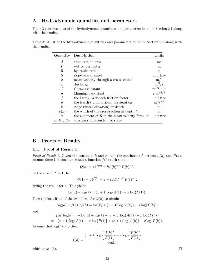
A Hydrodynamic quantities and parameters
Table 3 contains a list of the hydrodynamic quantities and parameters found in Section 2.1 alongwith their units.
Table 3: A list of the hydrodynamic quantities and parameters found in Section 2.1 along withtheir units.
Quantity Description Units
A cross section area m2
P wetted perimeter mR hydraulic radius mS slope of a channel unit freev mean velocity through a cross section m/sQ discharge m3/sC Chezy’s constant m1/2 s−1
n Manning’s constant s m−1/3
f the Darcy–Weisbach friction factor unit freeg the Earth’s gravitational acceleration m/s−2
h stage (water elevation) or depth mw(h) the width of the cross-section at depth h mx the exponent of R in the mean velocity formula unit free
k, K1, K2 constants independent of stage
B Proofs of Results
B.1 Proof of Result 1
Proof of Result 1. Given the constants k and x, and the continuous functions A(h) and P (h),assume there is a constant a and a function f(h) such that
Q(h) = ahf(h) = kA(h)x+1P (h)−x.
In the case of h = 1 then
Q(1) = a1f(1) = a = kA(1)x+1P (1)−x,
giving the result for a. This yields
log(a)− log(k) = (x+ 1) log{A(1)} − x log{P (1)}.Take the logarithm of the two forms for Q(h) to obtain
log(a) + f(h) log(h) = log(k) + (x+ 1) log{A(h)} − x log{P (h)}and
f(h) log(h) = − log(a) + log(k) + (x+ 1) log{A(h)} − x log{P (h)}= −(x+ 1) log{A(1)}+ x log{P (1)}+ (x+ 1) log{A(h)} − x log{P (h)}.
Assume that log(h) 6= 0 then
f(h) =
(x+ 1) log
{A(h)
A(1)
}− x log
{P (h)
P (1)
}
log(h)
which gives (5).
22

B.2 Proof of Result 2
Proof of Result 2. Note that
A′(h) =ddhA(h) =
ddh
∫ h
0(w1(η) + w2(η))dη = w1(η) + w2(η),
A′′(h) =ddhA′(h) = w′1(η) + w′2(η),
P ′(h) =ddhP (h) =
ddh
∫ h
0
√1 + {w′1(η)}2dη +
ddh
∫ h
0
√1 + {w′2(η)}2dη
=√
1 + {w′1(h)}2 +√
1 + {w′2(h)}2,
P ′′(h) =ddhP ′(h) =
ddh
√1 + {w′1(h)}2 +
ddh
√1 + {w′2(h)}2
=w′1(h)w′′1(h)√1 + {w′1(h)}2
+w′2(h)w′′2(h)√1 + {w′2(h)}2
.
The limit of f(h) as h approaches 1 can be evaluated using L’Hôpital’s rule once. That is,
limh→1
f(h) = limh→1
(x+ 1){logA(h)− logA(1)} − x{logP (h)− x logP (1)}log h
= limh→1
(x+ 1)A′(h)A(h)−1 − xP ′(h)P (h)−1
h−1
= (x+ 1)A′(1)
A(1)− xP
′(1)
P (1),
which gives (8). The limits of f(h) as h approaches zero from above and infinity can be evaluatedusing L’Hôpital’s rule twice. In the case of the limit where h approaches zero from above thenafter applying L’Hôpital’s rule once then
limh→0+
f(h) = limh→0+
(x+ 1)A′(h)A(h)−1 − xP ′(h)P (h)−1
h−1
= (x+ 1) limh→0+
hA′(h)
A(h)− x lim
h→0+
hP ′(h)
P (h)
= (x+ 1) limh→0+
{A′(h) + hA′′(h)}A′(h)
− x limh→0+
{P ′(h) + hP ′′(h)}P ′(h)
= (x+ 1) limh→0+
{1 +
hA′′(h)
A′(h)
}− x lim
h→0+
{1 +
hP ′′(h)
P ′(h)
}
= 1 + (x+ 1) limh→0+
hA′′(h)
A′(h)− x lim
h→0+
hP ′′(h)
P ′(h),
which gives (7).The proof for the limit of f(h) as h approaches infinity, which is given in (9), is similar as
it is also based on applying L’Hôpital’s rule twice. The main difference is that in the case of happroaching infinity the functions in both the numerator and the dominator approach infinitywhile in the case of h approaching zero from above the functions in both the numerator and thedominator approach zero; however, L’Hôpital’s rule is applicable in both cases.
23
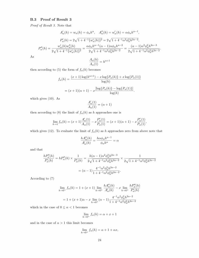
B.3 Proof of Result 3
Proof of Result 3. Note that
A′α(h) = wα(h) = φαhα, A′′α(h) = w′α(h) = αφαh
α−1,
P ′α(h) = 2√
1 + 4−1{w′α(h)}2 = 2√
1 + 4−1α2φ2αh2α−2,
P ′′α(h) =w′α(h)w′′α(h)
2√
1 + 4−1{w′α(h)}2=αφαh
α−1(α− 1)αφαhα−2
2√
1 + 4−1α2φ2αh2α−2 =
(α− 1)α2φ2αh2α−3
2√
1 + 4−1α2φ2αh2α−2 .
AsAα(h)
Aα(1)= hα+1
then according to (5) the form of fα(h) becomes
fα(h) =(x+ 1) log(hα+1)− x log{Pα(h)}+ x log{Pα(1)}
log(h)
= (x+ 1)(α+ 1)− x [log{Pα(h)} − log{Pα(1)}]log(h)
.
which gives (10). AsA′α(1)
Aα(1)= (α+ 1)
then according to (8) the limit of fα(h) as h approaches one is
limh→1
fα(h) = (x+ 1)A′α(1)
Aα(1)− xP
′α(1)
Pα(1)= (x+ 1)(α+ 1)− xP
′α(1)
Pα(1),
which gives (12). To evaluate the limit of fα(h) as h approaches zero from above note that
hA′′α(h)
A′α(h)=hαφαh
α−1
φαhα= α
and that
hP ′′α(h)
P ′α(h)= hP ′′α(h)× 1
P ′α(h)=
h(α− 1)α2φ2αh2α−3
2√
1 + 4−1α2φ2αh2α−2 ×
1
2√
1 + 4−1α2φ2αh2α−2
= (α− 1)4−1α2φ2αh
2α−2
1 + 4−1α2φ2αh2α−2 .
According to (7)
limh→0+
fα(h) = 1 + (x+ 1) limh→0+
hA′′α(h)
A′α(h)− x lim
h→0+
hP ′′α(h)
P ′α(h)
= 1 + (x+ 1)α− x limh→0+
(α− 1)4−1α2φ2αh
2α−2
1 + 4−1α2φ2αh2α−2
which in the case of 0 ≤ α < 1 becomes
limh→0+
fα(h) = α+ x+ 1
and in the case of α > 1 this limit becomes
limh→0+
fα(h) = α+ 1 + αx,
24
which gives (11). Same arguments can be used to show that the limit of fα(h) as h approachesinfinity in the case of 0 ≤ α < 1 becomes
limh→∞
fα(h) = α+ 1 + αx
and in the case of α > 1 the limit becomes
limh→∞
fα(h) = α+ x+ 1,
which gives (13). It was shown in the main text that the special case α = 1 resulted in a constantexponent, that is, f1(h) = 2 + x for h ≥ 0.
C The uncertainty in model comparison
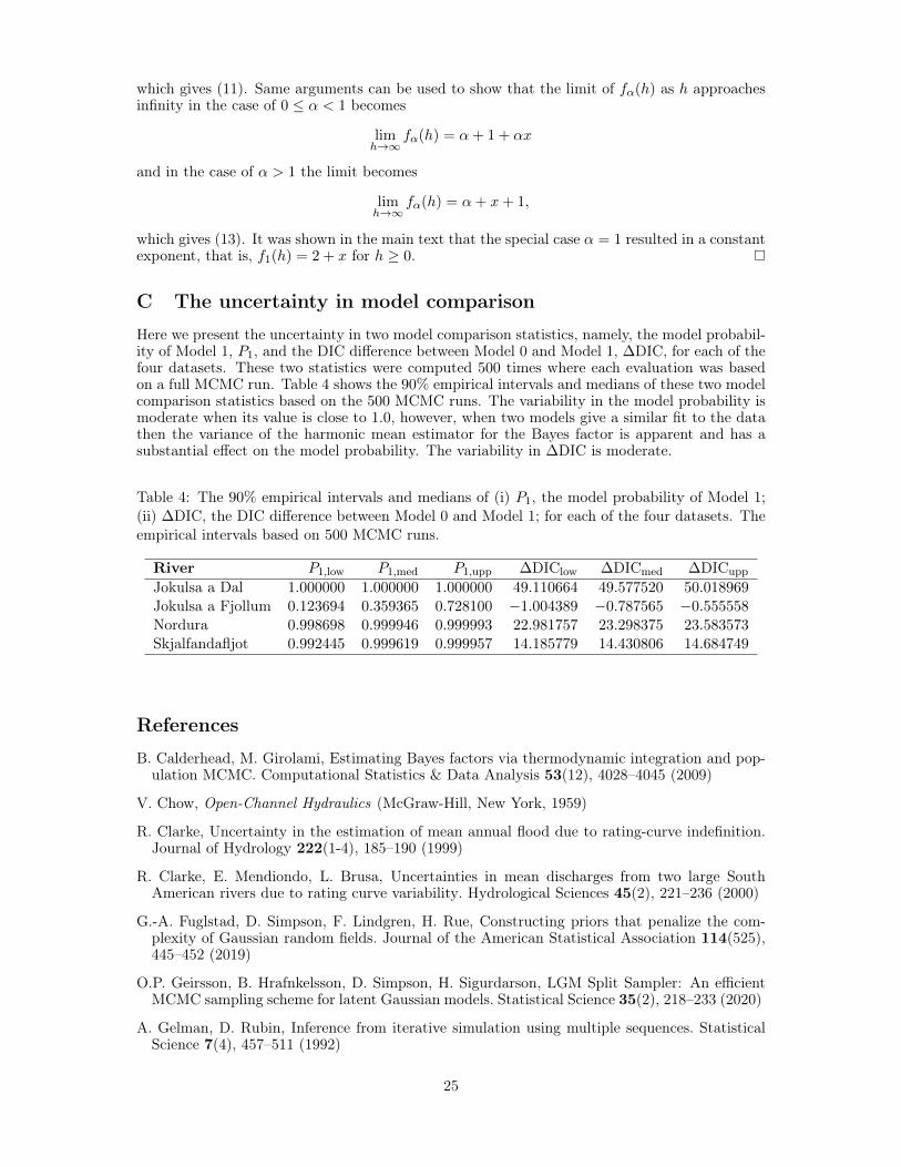
Here we present the uncertainty in two model comparison statistics, namely, the model probabil-ity of Model 1, P1, and the DIC difference between Model 0 and Model 1, ∆DIC, for each of thefour datasets. These two statistics were computed 500 times where each evaluation was basedon a full MCMC run. Table 4 shows the 90% empirical intervals and medians of these two modelcomparison statistics based on the 500 MCMC runs. The variability in the model probability ismoderate when its value is close to 1.0, however, when two models give a similar fit to the datathen the variance of the harmonic mean estimator for the Bayes factor is apparent and has asubstantial effect on the model probability. The variability in ∆DIC is moderate.
Table 4: The 90% empirical intervals and medians of (i) P1, the model probability of Model 1;(ii) ∆DIC, the DIC difference between Model 0 and Model 1; for each of the four datasets. Theempirical intervals based on 500 MCMC runs.
River P1,low P1,med P1,upp ∆DIClow ∆DICmed ∆DICuppJokulsa a Dal 1.000000 1.000000 1.000000 49.110664 49.577520 50.018969Jokulsa a Fjollum 0.123694 0.359365 0.728100 −1.004389 −0.787565 −0.555558Nordura 0.998698 0.999946 0.999993 22.981757 23.298375 23.583573Skjalfandafljot 0.992445 0.999619 0.999957 14.185779 14.430806 14.684749
References
B. Calderhead, M. Girolami, Estimating Bayes factors via thermodynamic integration and pop-ulation MCMC. Computational Statistics & Data Analysis 53(12), 4028–4045 (2009)
V. Chow, Open-Channel Hydraulics (McGraw-Hill, New York, 1959)
R. Clarke, Uncertainty in the estimation of mean annual flood due to rating-curve indefinition.Journal of Hydrology 222(1-4), 185–190 (1999)
R. Clarke, E. Mendiondo, L. Brusa, Uncertainties in mean discharges from two large SouthAmerican rivers due to rating curve variability. Hydrological Sciences 45(2), 221–236 (2000)
G.-A. Fuglstad, D. Simpson, F. Lindgren, H. Rue, Constructing priors that penalize the com-plexity of Gaussian random fields. Journal of the American Statistical Association 114(525),445–452 (2019)
O.P. Geirsson, B. Hrafnkelsson, D. Simpson, H. Sigurdarson, LGM Split Sampler: An efficientMCMC sampling scheme for latent Gaussian models. Statistical Science 35(2), 218–233 (2020)
A. Gelman, D. Rubin, Inference from iterative simulation using multiple sequences. StatisticalScience 7(4), 457–511 (1992)
25
A. Gelman, J. Carlin, H. Stern, D. Dunson, A. Vehtari, D. Rubin, Bayesian Data Analysis, 3rdedn. (Chapman & Hall/CRC Press, Boca Raton, FL, 2013)
G. Gioia, F. Bombardelli, Scaling and similarity in rough channel flows. Physical Review Letters88(1), 1–4 (2001)
R. Herschy, Streamflow Measurement, 3rd edn. (Taylor & Francis, Oxford, 2009)
B. Hrafnkelsson, K. Ingimarsson, S. Gardarsson, A. Snorrason, Modeling discharge rating curveswith Bayesian B-splines. Stochastic Environmental Research and Risk Assessment 26(1), 1–20(2012)
R. Jarrett, Hydraulics of high-gradient streams. Journal of Hydraulic Engineering 110(11), 1519–1539 (1984)
H. Jeffreys, Theory of Probability, 3rd edn. (Oxford University Press, Oxford, 1961)
R. Kass, A. Raftery, Bayes Factors. Journal of the American Statistical Association 90, 773–795(1995)
L. Knorr-Held, H. Rue, On block updating in Markov random field models for disease mapping.Scandinavian Journal of Statistics 29(4), 597–614 (2002)
M. Meis, M.P. Llano, D. Rodriguez, Quantifying and modelling the ENSO phe-nomenon and extreme discharge events relation in the La Plata Basin. Hydro-logical Sciences Journal 66(1), 75–89 (2021). doi:10.1080/02626667.2020.1843655.https://doi.org/10.1080/02626667.2020.1843655
M. Mosley, A. McKerchar, Streamflow. Chapter 8, in Handbook of Hydrology, ed. by D. Maidment(McGraw-Hill, New York, 1993)
R. Moyeed, R. Clarke, The use of Bayesian methods for fitting rating curves, with case studies.Advances in Water Resources 28(8), 807–818 (2005)
M.A. Newton, A.E. Raftery, Approximate Bayesian inference with the weighted likelihood boot-strap. Journal of the Royal Statistical Society: Series B (Methodological) 56(1), 3–26 (1994)
A. Petersen-Øverleir, Accounting for heteroscedasticity in rating curve estimates. Journal ofHydrology 292(1-4), 173–181 (2004)
A. Petersen-Øverleir, Modelling stage-discharge relationships affected by hysteresis using theJones formula and nonlinear regression. Hydrological Sciences Journal 51(3), 365–388 (2006)
A. Petersen-Øverleir, Fitting depth-discharge relationships in rivers with floodplains. HydrologyResearch 39(5-6), 369–384 (2008)
A. Petersen-Øverleir, T. Reitan, Objective segmentation in compound rating curves. Journal ofHydrology 311(1-4), 188–201 (2005)
I. Popescu, L. Brandimarte, M. Peviani, Effects of climate change over energy production inLa Plata Basin. International Journal of River Basin Management 12(4), 319–327 (2014).doi:10.1080/15715124.2014.917317. https://doi.org/10.1080/15715124.2014.917317
A. Raftery, M. Newton, J. Satagopan, P. Krivitsky, Estimating the integrated likelihood viaposterior simulation using the harmonic mean identity. Bayesian Statistics 8, 1–45 (2007)
T. Reitan, A. Petersen-Øverleir, Existence of the frequentistic estimate for power-law regressionwith a location parameter, with applications for making discharge rating curves. StochasticEnvironmental Research and Risk Assessment 20(6), 445–453 (2006)
T. Reitan, A. Petersen-Øverleir, Bayesian power-law regression with a location parameter, withapplications for construction of discharge rating curves. Stochastic Environmental Researchand Risk Assessment 22(3), 351–365 (2007)
26

T. Reitan, A. Petersen-Øverleir, Bayesian methods for estimating multi-segment discharge ratingcurves. Stochastic Environmental Research and Risk Assessment 23(5), 627–642 (2008)
G.O. Roberts, A. Gelman, W.R. Gilks, Weak convergence and optimal scaling of random walkMetropolis algorithms. The Annals of Applied Probability 7(1), 110–120 (1997)
H. Rue, L. Held, Gaussian Markov Random Fields: Theory and Applications (Chapman &Hall/CRC Press, Boca Raton, FL, 2005)
H. Shen, P. Julien, Erosion and Sediment Transport. Chapter 12, in Handbook of Hydrology, ed.by D. Maidment (McGraw-Hill, New York, 1993)
D. Simpson, H. Rue, A. Riebler, T.G. Martins, S.H. Sørbye, Penalising model component com-plexity: A principled, practical approach to constructing priors. Statistical Science 32(1), 1–28(2017)
D. Spiegelhalter, N. Best, B. Carlin, A. Van Der Linde, Bayesian measures of model complexityand fit. Journal of the Royal Statistical Society: Series B (Statistical Methodology) 64(4),583–639 (2002)
C. Venetis, A note on the estimation of the parameters in logarithmic stage-discharge relation-ships with estimates of their error. International Association of Scientific Hydrology. BulletinXV 2(6), 105–111 (1970)
Y.-H. Wang, Y.-S. Zou, L.-Q. Xu, Z. Luo, Analysis of water flow pressure on bridge piersconsidering the impact effect. Mathematical Problems in Engineering 2015, 687535 (2015).doi:10.1155/2015/687535. https://doi.org/10.1155/2015/687535
L. Wassermann, All of Nonparametric Statistics (Springer, New York, 2006)
27
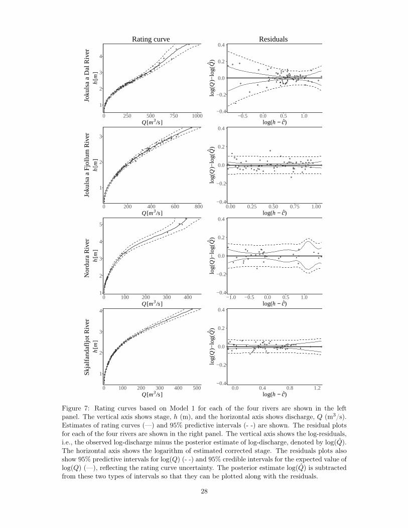
1
2
3
4
0 250 500 750 1000Q[m3/s]
h[m
]
Rating curve
Joku
lsa
a D
al R
iver
−0.4
−0.2
0.0
0.2
0.4
−0.5 0.0 0.5 1.0log(h − c)
log(
Q)−
log(
Q)
Residuals
1
2
3
0 200 400 600 800Q[m3/s]
h[m
]Jo
kuls
a a
Fjo
llum
Riv
er
−0.4
−0.2
0.0
0.2
0.4
0.00 0.25 0.50 0.75 1.00log(h − c)
log(
Q)−
log(
Q)
1
2
3
4
5
0 100 200 300 400Q[m3/s]
h[m
]N
ordu
ra R
iver
−0.4
−0.2
0.0
0.2
0.4
−1.0 −0.5 0.0 0.5 1.0log(h − c)
log(
Q)−
log(
Q)
1
2
3
4
0 100 200 300 400 500Q[m3/s]
h[m
]S
kjal
fand
afljo
t Riv
er
−0.4
−0.2
0.0
0.2
0.4
0.0 0.4 0.8 1.2log(h − c)
log(
Q)−
log(
Q)
Figure 7: Rating curves based on Model 1 for each of the four rivers are shown in the leftpanel. The vertical axis shows stage, h (m), and the horizontal axis shows discharge, Q (m3/s).Estimates of rating curves (—) and 95% predictive intervals (- -) are shown. The residual plotsfor each of the four rivers are shown in the right panel. The vertical axis shows the log-residuals,i.e., the observed log-discharge minus the posterior estimate of log-discharge, denoted by log(Q).The horizontal axis shows the logarithm of estimated corrected stage. The residuals plots alsoshow 95% predictive intervals for log(Q) (- -) and 95% credible intervals for the expected value oflog(Q) (—), reflecting the rating curve uncertainty. The posterior estimate log(Q) is subtractedfrom these two types of intervals so that they can be plotted along with the residuals.
28
Supplementary material for: "Generalization of the power-lawrating curve using hydrodynamic theory and Bayesian
hierarchical modeling"
Birgir Hrafnkelsson,1∗ Helgi Sigurdarson,2 Sölvi Rögnvaldsson,1
Axel Örn Jansson,1 Rafael Daníel Vias,1 Sigurdur Magnus Gardarsson1
1University of Iceland,2Isavia, Iceland
1 Convergence assessment
Trace plots and histograms of four parameters in Model 0 for the Jokulsa a Fjollum River areshown in Figure 1 and Figure 2 shows the autocorrelation function and the Gelman–Rubinstatistic for the same parameters when using the same dataset. Figure 3 shows the trace plotsand histograms of four parameters in Model 1 for the Jokulsa a Dal River. Figure 4 showsthe autocorrelation function and the Gelman–Rubin statistic for the same parameters and thesame dataset. Results for other parameters in Model 0 and Model 1, and results based on theNordura River dataset and the Skjalfandi River dataset are not shown. However, the convergencediagnostics plots for these parameters were the similar those shown in Figures 1, 2, 3 and 4.
The Gelman–Rubin statistic plots show the rate of convergence with the value 1.1 as areference point. Values above 1.1 indicate that sufficient convergence has not been reached. Traceplots and the autocorrelation function indicate the quality of simulated chains. A slowly decayingautocorrelation function indicates worse quality. Trace plots show how well the chains mix. A badmixing of chains indicates worse quality. An example of a bad mixing is separate chains stayingin separate regions over a large number of consecutive iterations and never crossing. Histogramsgive the marginal distributions under the assumption that convergence has been reached. Figures1, 2, 3 and 4 show that convergence according to the Gelman–Rubin statistic was reached after10000 iterations (after burn-in), the autocorrelation between samples 50 iterations apart (nothinning applied) was less than 0.2, and the chains of both Model 0 and Model 1 mix well.
1
arX
iv:2
010.
0476
9v2
[st
at.A
P] 9
Aug
202
1
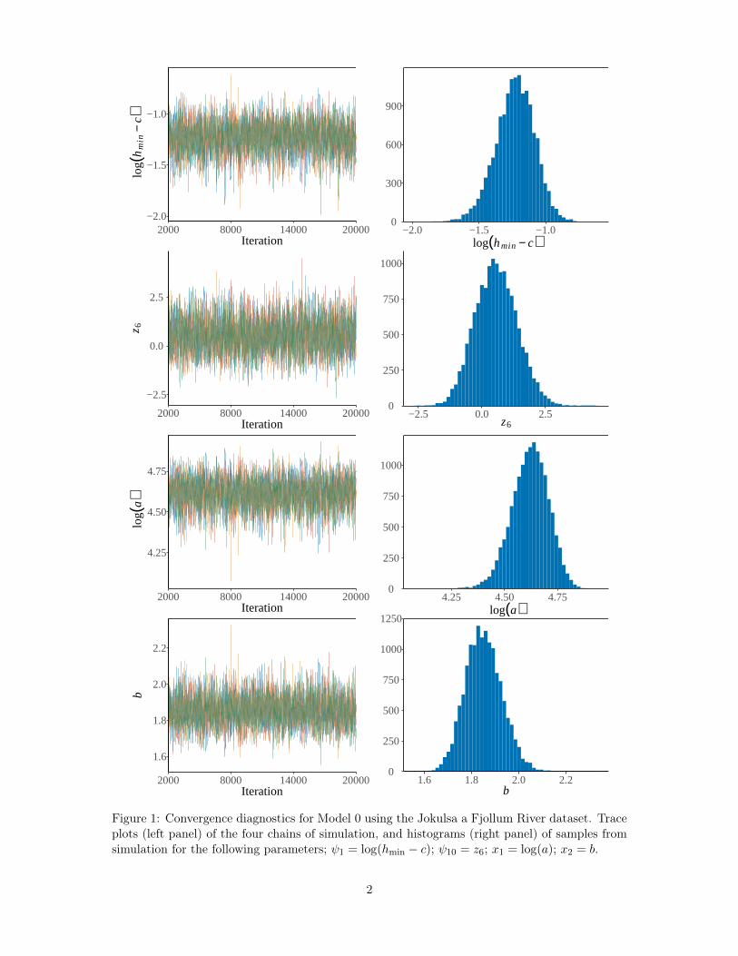
−2.0
−1.5
−1.0
2000 8000 14000 20000Iteration
log(
hm
in−
c)
−2.5
0.0
2.5
2000 8000 14000 20000Iteration
z 6
4.25
4.50
4.75
2000 8000 14000 20000Iteration
log(
a)
1.6
1.8
2.0
2.2
2000 8000 14000 20000Iteration
b
−2.0 −1.5 −1.00
300
600
900
log(hmi n − c)
−2.5 0.0 2.50
250
500
750
1000
z6
4.25 4.50 4.750
250
500
750
1000
log(a)
1.6 1.8 2.0 2.20
250
500
750
1000
1250
b
Figure 1: Convergence diagnostics for Model 0 using the Jokulsa a Fjollum River dataset. Traceplots (left panel) of the four chains of simulation, and histograms (right panel) of samples fromsimulation for the following parameters; ψ1 = log(hmin − c); ψ10 = z6; x1 = log(a); x2 = b.
2
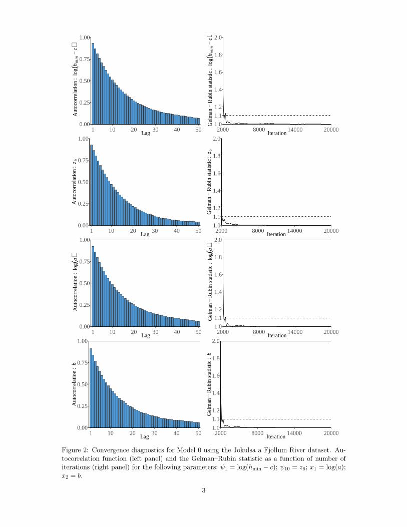
0.00
0.25
0.50
0.75
1.00
1 10 20 30 40 50Lag
Aut
ocor
rela
tion
: lo
g(h
min
−c)
0.00
0.25
0.50
0.75
1.00
1 10 20 30 40 50Lag
Aut
ocor
rela
tion
: z 6
0.00
0.25
0.50
0.75
1.00
1 10 20 30 40 50Lag
Aut
ocor
rela
tion
: lo
g(a)
0.00
0.25
0.50
0.75
1.00
1 10 20 30 40 50Lag
Aut
ocor
rela
tion
: b
1.0
1.1
1.2
1.4
1.6
1.8
2.0
2000 8000 14000 20000Iteration
Gel
man
−R
ubin
stat
istic
: lo
g(h
min
−c)
1.0
1.1
1.2
1.4
1.6
1.8
2.0
2000 8000 14000 20000Iteration
Gel
man
−R
ubin
stat
istic
: z 6
1.0
1.1
1.2
1.4
1.6
1.8
2.0
2000 8000 14000 20000Iteration
Gel
man
−R
ubin
stat
istic
: lo
g(a)
1.0
1.1
1.2
1.4
1.6
1.8
2.0
2000 8000 14000 20000Iteration
Gel
man
−R
ubin
stat
istic
: b
Figure 2: Convergence diagnostics for Model 0 using the Jokulsa a Fjollum River dataset. Au-tocorrelation function (left panel) and the Gelman–Rubin statistic as a function of number ofiterations (right panel) for the following parameters; ψ1 = log(hmin − c); ψ10 = z6; x1 = log(a);x2 = b.
3
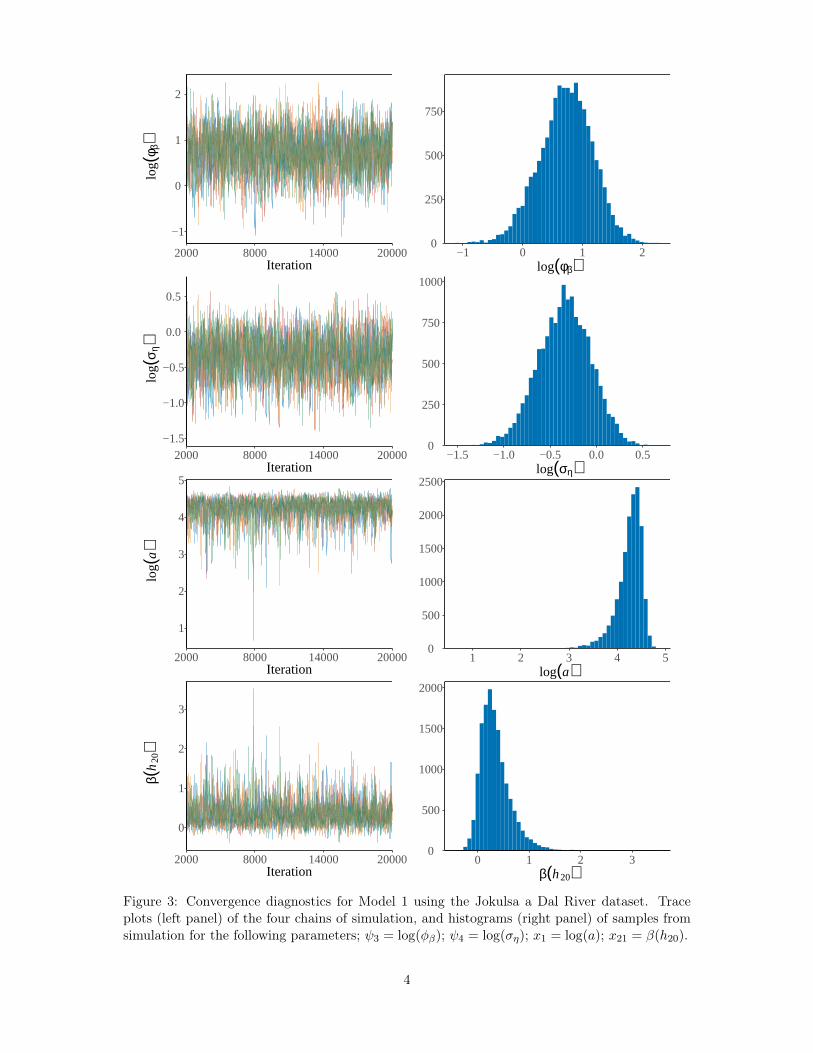
−1
0
1
2
2000 8000 14000 20000Iteration
log(
φ β)
−1.5
−1.0
−0.5
0.0
0.5
2000 8000 14000 20000Iteration
log(
σ η)
1
2
3
4
5
2000 8000 14000 20000Iteration
log(
a)
0
1
2
3
2000 8000 14000 20000Iteration
β(h
20)
−1 0 1 20
250
500
750
log(φβ)
−1.5 −1.0 −0.5 0.0 0.50
250
500
750
1000
log(ση)
1 2 3 4 50
500
1000
1500
2000
2500
log(a)
0
500
1000
1500
2000
0 1 2 3β(h20)
Figure 3: Convergence diagnostics for Model 1 using the Jokulsa a Dal River dataset. Traceplots (left panel) of the four chains of simulation, and histograms (right panel) of samples fromsimulation for the following parameters; ψ3 = log(φβ); ψ4 = log(ση); x1 = log(a); x21 = β(h20).
4
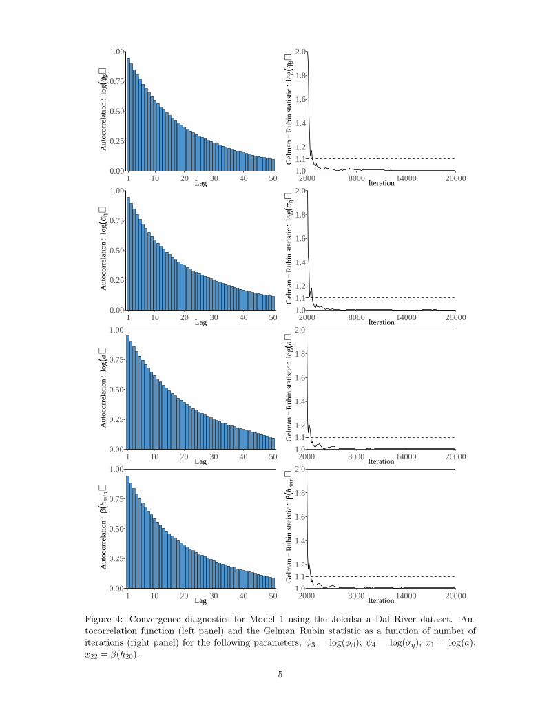
0.00
0.25
0.50
0.75
1.00
1 10 20 30 40 50Lag
Aut
ocor
rela
tion
: lo
g(φ β
)
0.00
0.25
0.50
0.75
1.00
1 10 20 30 40 50Lag
Aut
ocor
rela
tion
: lo
g(σ η
)
0.00
0.25
0.50
0.75
1.00
1 10 20 30 40 50Lag
Aut
ocor
rela
tion
: lo
g(a)
0.00
0.25
0.50
0.75
1.00
1 10 20 30 40 50Lag
Aut
ocor
rela
tion
: β(
hm
in)
1.0
1.1
1.2
1.4
1.6
1.8
2.0
2000 8000 14000 20000Iteration
Gel
man
−R
ubin
stat
istic
: lo
g(φ β
)
1.0
1.1
1.2
1.4
1.6
1.8
2.0
2000 8000 14000 20000Iteration
Gel
man
−R
ubin
stat
istic
: lo
g(σ η
)
1.0
1.1
1.2
1.4
1.6
1.8
2.0
2000 8000 14000 20000Iteration
Gel
man
−R
ubin
stat
istic
: lo
g(a)
1.0
1.1
1.2
1.4
1.6
1.8
2.0
2000 8000 14000 20000Iteration
Gel
man
−R
ubin
stat
istic
: β(
hm
in)
Figure 4: Convergence diagnostics for Model 1 using the Jokulsa a Dal River dataset. Au-tocorrelation function (left panel) and the Gelman–Rubin statistic as a function of number ofiterations (right panel) for the following parameters; ψ3 = log(φβ); ψ4 = log(ση); x1 = log(a);x22 = β(h20).
5


