
IMAGE RESTORATION
Image restoration
SUMMARY:
• Summary of frequency domain filtering
• Linear degradation model
• Linear restoration model
• Linear shift-invariant systems
• Inverse filter
• Parametric Wiener filter
1
Image restoration
Process of removing or reducing image degradations whichoccur during image formation.
2
Image degradation
Degrading factors:
• blurring produced by the optical system or object motion duringacquisition
• noise from electronic and optical devices.
3

Restoration
• Noise only: spatial filtering, frequency filtering
• Linear shift-invariant (LSI) degradations
4
Noise models
Gaussian; Rayleigh; Gamma; Exponential; Uniform; Impulse(shot noise).
5
Noise only filtering
Degraded image g(x, y) :
g(x, y) = f(x, y) + η(x, y)
• Mean filter: f̂(x, y) = 1mn
∑(s,t)∈Sxy g(s, t)
• Median filter: f̂(x, y) = median(s,t)∈Sxy g(s, t)
• Bandreject frequency domain filters
6
Linear shift-invariant systems
A linear shift-invariant (LSI) system O maps an input signal f(t)to an output signal g(t), denoted as f(t) O→ g(t), satisfying:
• Linearity: if f1(t)O→ g1(t) and f2(t)
O→ g2(t), then, for arbitraryconstants a, b,
a f1(t) + b f2(t)O→ a g1(t) + b g2(t)
• Shift invariance: if f(t) O→ g(t), then for each time shift T ,
f(t− T ) O→ g(t− T )
7

Convolution
• Output of a LSI system is given by the convolution of the inputwith a kernel h(t):
g(t) = (h ∗ f)(t) =∫ ∞
−∞h(t− s) f(s) ds
• Filter kernel h(t) is called the impulse response function or in2-D point spread function.
• The Fourier transform H(µ) is called the transfer function.
8
Linear shift-invariant degradations
• Degraded image g(x, y) is convolution of ideal image f(x, y)by kernel h(x, y) plus noise η(x, y):
g(x, y) = (h ∗ f)(x, y) + η(x, y).
In frequency domain:
G(u, v) = H(u, v)F (u, v) +N(u, v)
• Finite images of size N ×N :
g = Hf + n
where g, f ,n are column vectors of length M × N , and H isan MN ×MN convolution matrix.
9
Linear restoration model
Deconvolution: compute an estimate f̂(x, y) of the ideal imageby using a reconstruction kernel r(x, y):
f̂(x, y) = (r ∗ g)(x, y)
h
hg ^
10
Constrained least squares restoration
• Solution Estimated solution f̂ should satisfy the model equation:∥∥∥g −Hf̂
∥∥∥2
= ‖n‖2
• Constraints: introducing a matrix Q such that the term∥∥∥Q f̂
∥∥∥2
is minimized.
11

Minimization problem and solution
• Minimize
E(f̂) = K∥∥∥Q f̂
∥∥∥2
+
(∥∥∥g −Hf̂∥∥∥2
− ‖n‖2)
where K is a constant, called the regularization parameter,which determines the relative weight of both terms
• Least squares solution:
f̂ =(HtH+KQtQ
)−1Htg
12
Inverse filter
• Put K = 0 in formula for least squares solution:
f̂ = (HtH)−1Htg = H−1g
= H−1(Hf + n) = f +H−1n
Expressed in the frequency domain:
F̂ (u, v) = F (u, v) +N(u, v)
H(u, v)
This is the ‘inverse’ filter.
• This filter is useless in practice: small values in H(u, v) amplifythe noise.
13
Wiener filter
Assume f and n to be random vectors with zero mean andcovariance matrices Rf = E(f f t) for the signal and Rn = E(nnt)
for the noise. Let Q be the noise-to-signal ratio Q =(RnRf
)12
andlet K = 1.
f̂ =(HtH+R−1f Rn
)−1Htg
14
Parametric Wiener filter
Minimum norm least squares solution:
f̂ =(HtH+K I
)−1Htg
or, expressed in the frequency domain:
F̂ (u, v) =[ H∗(u, v)
|H(u, v)|2 +K
]G(u, v)
This is the Parametric Wiener filter or Pseudo-inverse filter.
K is the regularization parameter.
Case K = 0: inverse filter.
15
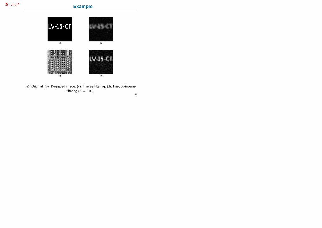
Example
(a): Original. (b): Degraded image. (c): Inverse filtering. (d): Pseudo-inversefiltering (K = 0.01).
16


