IntroductiontoAdvancedProbabilityforGraphicalModels
CSC412ByElliotCreager
ThursdayJanuary11,2018
PresentedbyJonathanLorraine
*ManyslidesbasedonKaustav Kundu’s, KevinSwersky’s,Inmar Givoni’s,DannyTarlow’s,JasperSnoek’s slides,SamRoweis ‘sreviewofprobability, Bishop’sbook,andsomeimagesfromWikipedia
Outline
• Basics• Probabilityrules• Exponentialfamilymodels• Maximumlikelihood• ConjugateBayesianinference(timepermitting)
WhyRepresentUncertainty?
• Theworldisfullofuncertainty– “Whatwilltheweatherbeliketoday?”– “WillIlikethismovie?”– “Isthereapersoninthisimage?”
• We’retryingtobuildsystemsthatunderstandand(possibly)interactwiththerealworld
• Weoftencan’tprovesomethingistrue,butwecanstillaskhowlikelydifferentoutcomesareoraskforthemostlikelyexplanation
• Sometimesprobabilitygivesaconcisedescriptionofanotherwisecomplexphenomenon.
WhyUseProbabilitytoRepresentUncertainty?
• Writedownsimple,reasonablecriteriathatyou'dwantfromasystemofuncertainty(commonsensestuff),andyoualwaysgetprobability.
• CoxAxioms(Cox1946);SeeBishop,Section1.2.3
• Wewillrestrictourselvestoarelativelyinformaldiscussionofprobabilitytheory.
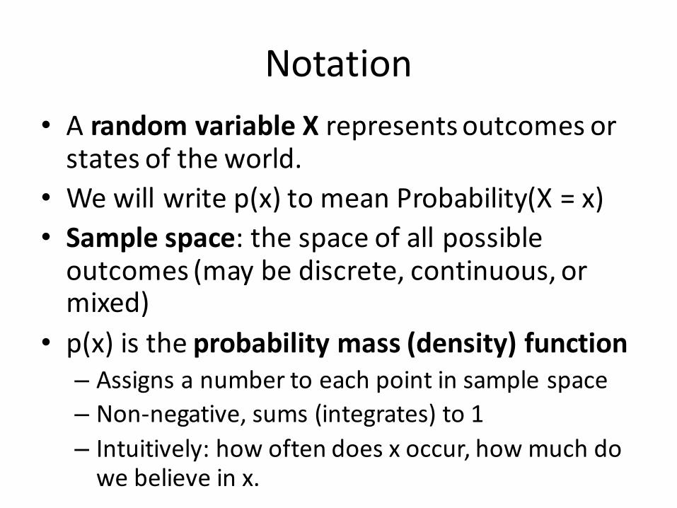
Notation• A randomvariableX representsoutcomesorstatesoftheworld.
• Wewillwritep(x)tomeanProbability(X=x)• Samplespace:thespaceofallpossibleoutcomes(maybediscrete,continuous,ormixed)
• p(x)istheprobabilitymass(density)function– Assignsanumbertoeachpointinsamplespace– Non-negative,sums(integrates)to1– Intuitively:howoftendoesxoccur,howmuchdowebelieveinx.
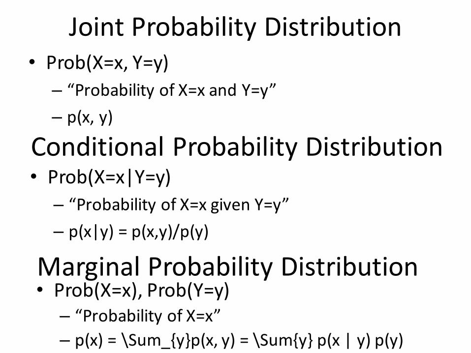
JointProbabilityDistribution• Prob(X=x,Y=y)– “ProbabilityofX=xandY=y”– p(x,y)
ConditionalProbabilityDistribution• Prob(X=x|Y=y)– “Probability ofX=xgivenY=y”– p(x|y)=p(x,y)/p(y)
MarginalProbabilityDistribution• Prob(X=x),Prob(Y=y)– “Probability ofX=x”– p(x)=\Sum_{y}p(x,y)=\Sum{y}p(x|y)p(y)
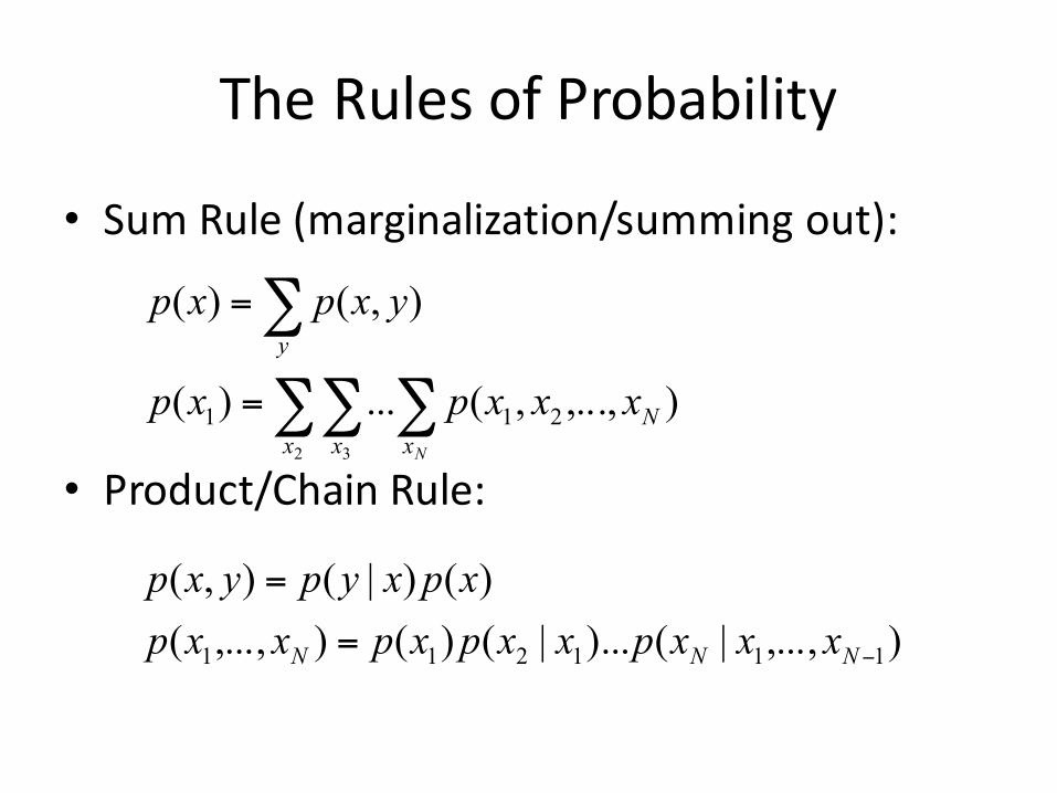
TheRulesofProbability
• SumRule(marginalization/summingout):
• Product/ChainRule:
),...,,(...)(
),()(
2112 3
Nx x x
y
xxxpxp
yxpxp
N
∑∑ ∑
∑
=
=
),...,|()...|()(),...,()()|(),(
111211 −=
=
NNN xxxpxxpxpxxpxpxypyxp
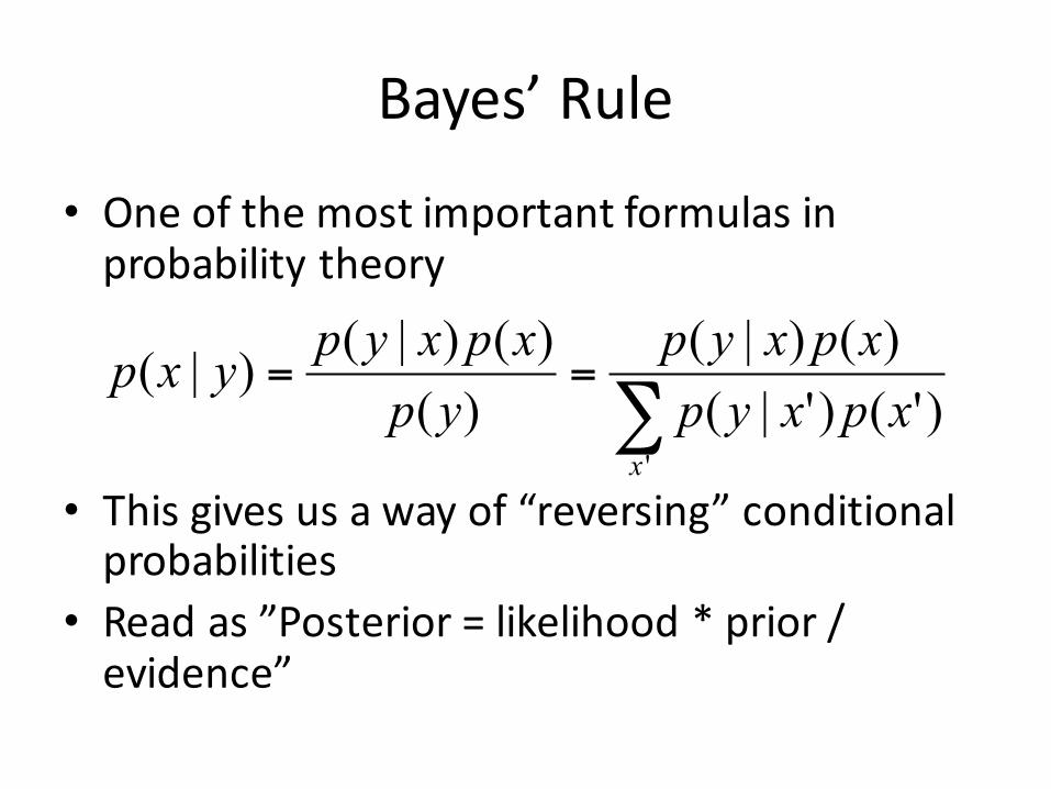
Bayes’Rule
• Oneofthemostimportantformulasinprobabilitytheory
• Thisgivesusawayof“reversing”conditionalprobabilities
• Readas”Posterior=likelihood*prior/evidence”
∑==
')'()'|(
)()|()()()|()|(
xxpxypxpxyp
ypxpxypyxp
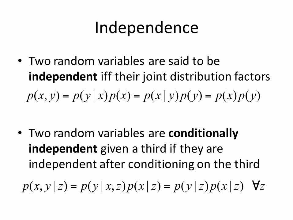
Independence
• Tworandomvariablesaresaidtobeindependent iff theirjointdistributionfactors
• Tworandomvariablesareconditionallyindependentgivenathirdiftheyareindependentafterconditioningonthethird
)()()()|()()|(),( ypxpypyxpxpxypyxp ===
zzxpzypzxpzxypzyxp ∀== )|()|()|(),|()|,(
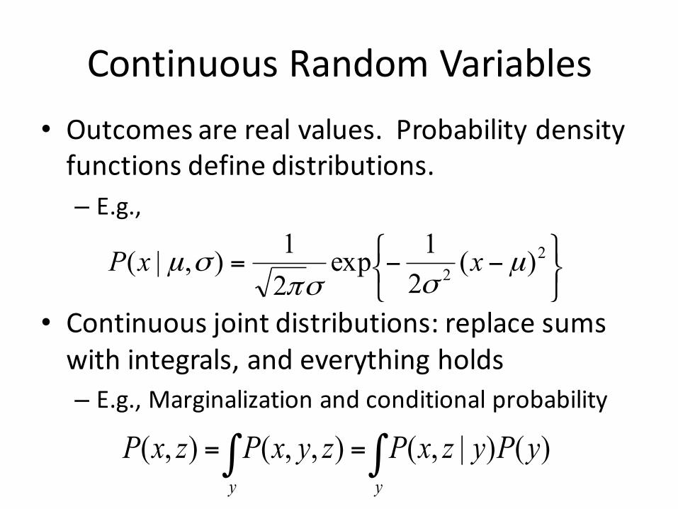
ContinuousRandomVariables• Outcomesarerealvalues.Probabilitydensityfunctionsdefinedistributions.– E.g.,
• Continuousjointdistributions:replacesumswithintegrals,andeverythingholds– E.g.,Marginalizationandconditionalprobability
∫∫ ==yy
yPyzxPzyxPzxP )()|,(),,(),(
⎭⎬⎫
⎩⎨⎧ −−= 2
2 )(21exp
21),|( µ
σσπσµ xxP
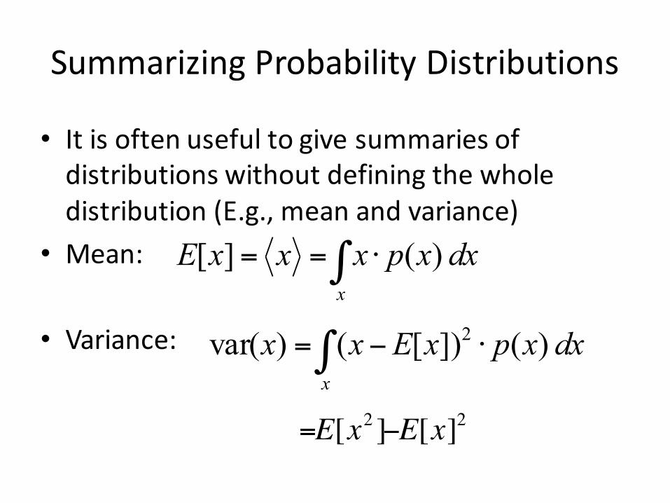
SummarizingProbabilityDistributions
• Itisoftenusefultogivesummariesofdistributionswithoutdefiningthewholedistribution(E.g.,meanandvariance)
• Mean:
• Variance:
dxxpxxxEx
)(][ ∫ ⋅==
dxxpxExxx
)(])[()var( 2∫ ⋅−=
=E[x2 ]−E[x]2
ExponentialFamily
• Familyofprobabilitydistributions• Manyofthestandarddistributionsbelongtothisfamily– Bernoulli,binomial/multinomial,Poisson,Normal(Gaussian),beta/Dirichlet,…
• Sharemanyimportantproperties– e.g. Theyhaveaconjugateprior(we’llgettothatlater.ImportantforBayesianstatistics)
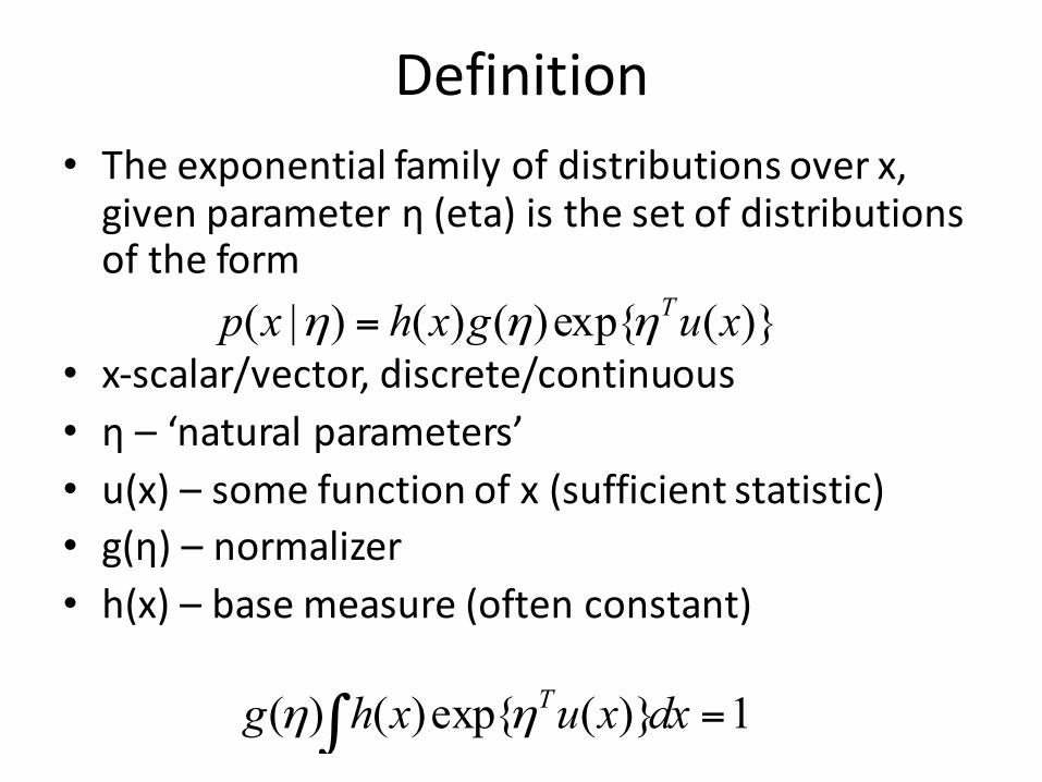
Definition• Theexponentialfamilyofdistributionsoverx,givenparameterη (eta)isthesetofdistributionsoftheform
• x-scalar/vector,discrete/continuous• η – ‘naturalparameters’• u(x)– somefunctionofx(sufficientstatistic)• g(η)– normalizer• h(x)– basemeasure(oftenconstant)
)}(exp{)()()|( xugxhxp Tηηη =
1)}(exp{)()( =∫ dxxuxhg Tηη
SufficientStatistics
• Vaguedefinition:calledsobecausetheycompletelysummarizeadistribution.
• Lessvague:theyaretheonlypartofthedistributionthatinteractswiththeparametersandarethereforesufficienttoestimatetheparameters.
• Perhapsthenumberoftimesacoincameupheads,orthesumofvaluesmagnitudes.
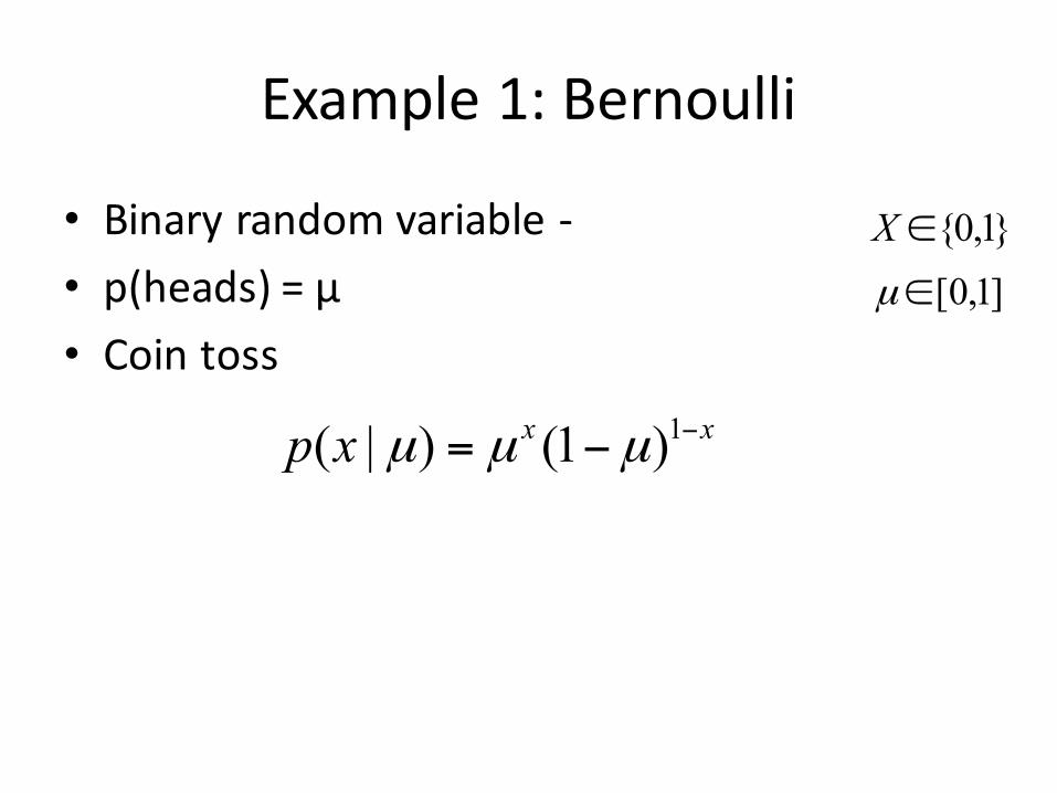
Example1:Bernoulli
• Binaryrandomvariable-• p(heads)=µ• Cointoss
xxxp −−= 1)1()|( µµµ
}1,0{∈X]1,0[∈µ
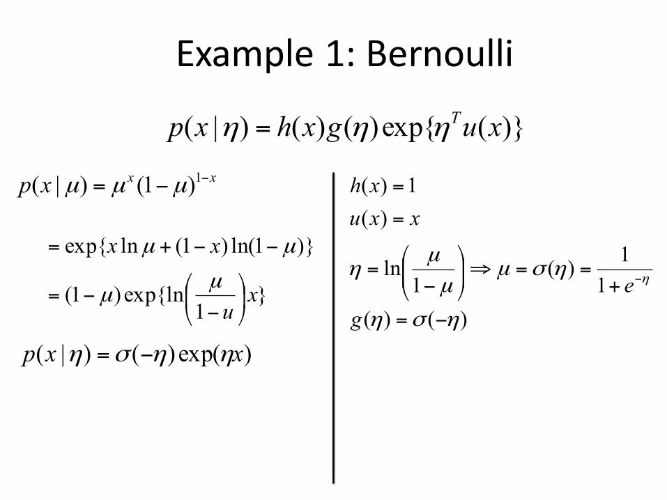
Example1:Bernoulli
xxxp −−= 1)1()|( µµµ
}1
exp{ln)1(
)}1ln()1(lnexp{
xu
xx
⎟⎠
⎞⎜⎝
⎛−
−=
−−+=
µµ
µµ
)()(11)(
1ln
)(1)(
ηση
ησµµµ
η η
−=
+==⇒⎟⎟
⎠
⎞⎜⎜⎝
⎛
−=
=
=
−
ge
xxuxh
)}(exp{)()()|( xugxhxp Tηηη =
)exp()()|( xxp ηηση −=
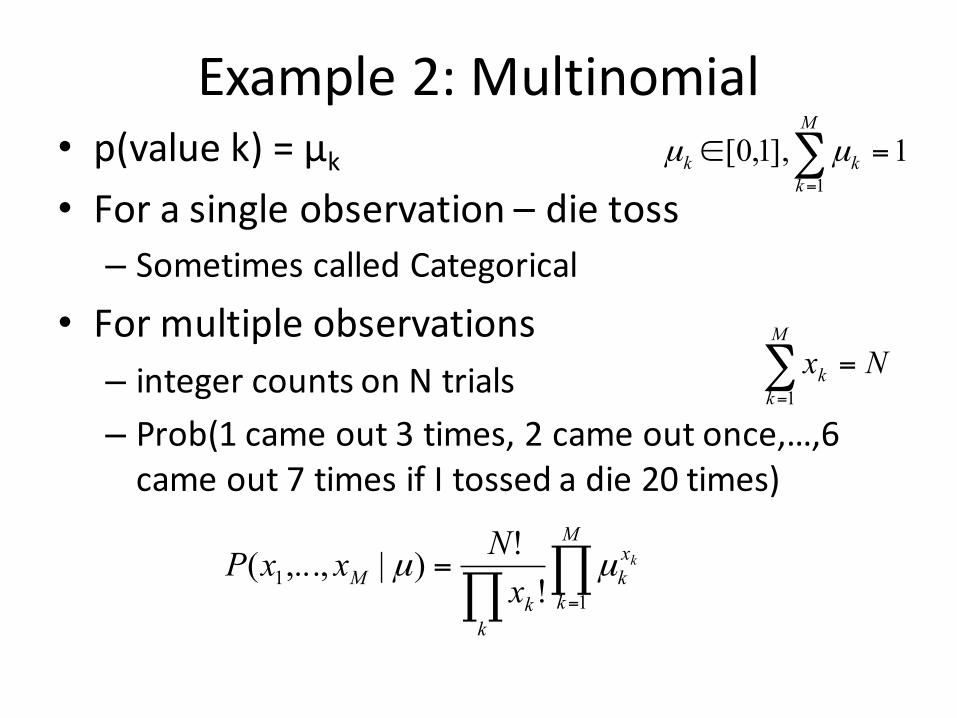
Example2:Multinomial• p(valuek)=µk
• Forasingleobservation– dietoss– SometimescalledCategorical
• Formultipleobservations– integercountsonNtrials– Prob(1cameout3times,2cameoutonce,…,6cameout7timesifItossedadie20times)
1],1,0[1
=∈ ∑=
M
kkk µµ
∏∏ =
=M
k
xk
kk
Mk
xNxxP
11 !
!)|,...,( µµ
∑=
=M
kk Nx
1
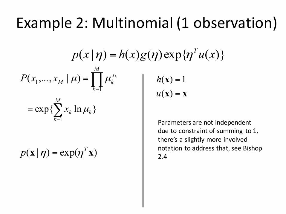
Example2:Multinomial(1observation)
}lnexp{1∑=
=M
kkkx µ
xxx=
=
)(1)(
uh
)}(exp{)()()|( xugxhxp Tηηη =
∏=
=M
k
xkMkxxP
11 )|,...,( µµ
)exp()|( xx Tp ηη =
Parametersarenotindependentduetoconstraintofsumming to1,there’saslightlymoreinvolvednotation toaddressthat,seeBishop2.4
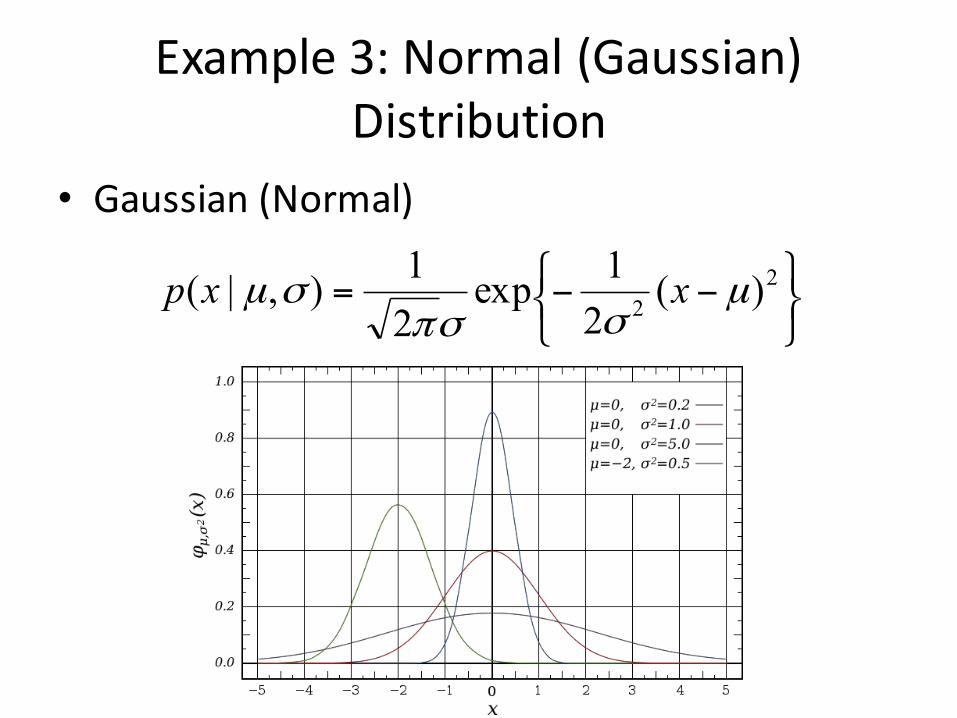
Example3:Normal(Gaussian)Distribution
• Gaussian(Normal)
⎭⎬⎫
⎩⎨⎧ −−= 2
2 )(21exp
21),|( µ
σσπσµ xxp
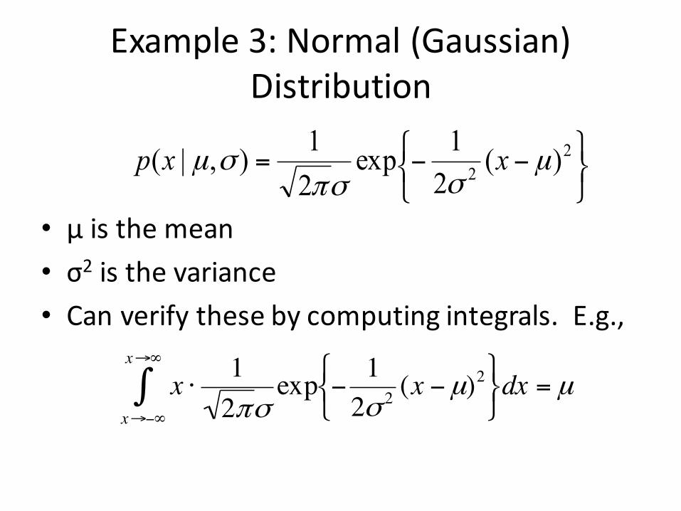
Example3:Normal(Gaussian)Distribution
• µisthemean• σ2 isthevariance• Canverifythesebycomputingintegrals.E.g.,
⎭⎬⎫
⎩⎨⎧ −−= 2
2 )(21exp
21),|( µ
σσπσµ xxp
€
x ⋅ 12πσ
exp −12σ 2 (x −µ)2
⎧ ⎨ ⎩
⎫ ⎬ ⎭ dx = µ
x→−∞
x→∞
∫
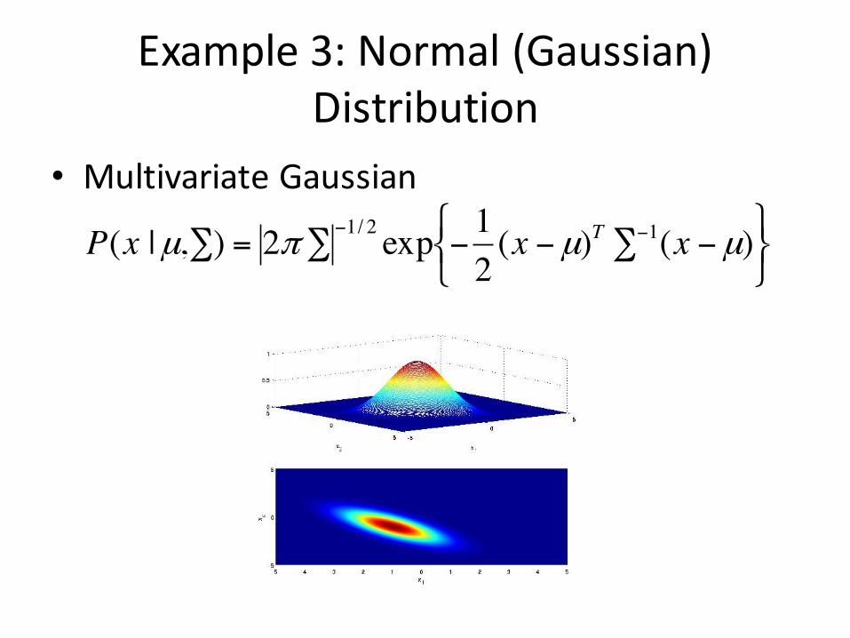
Example3:Normal(Gaussian)Distribution
• MultivariateGaussian
€
P(x |µ,∑) = 2π ∑−1/ 2 exp −12(x −µ)T ∑−1(x −µ)
⎧ ⎨ ⎩
⎫ ⎬ ⎭
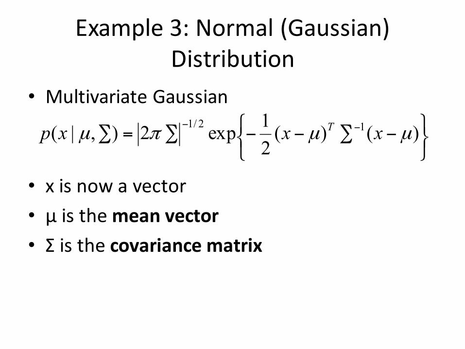
Example3:Normal(Gaussian)Distribution
• MultivariateGaussian
• x isnowavector• µisthemeanvector• Σ isthecovariancematrix
⎭⎬⎫
⎩⎨⎧ −∑−−∑=∑ −− )()(21exp2),|( 12/1
µµπµ xxxp T
ImportantPropertiesofGaussians
• Allmarginals ofaGaussianareagainGaussian• AnyconditionalofaGaussianisGaussian• TheproductoftwoGaussiansisagainGaussian
• EventhesumoftwoindependentGaussianRVsisaGaussian.
• Beyondthescopeofthistutorial,butveryimportant:marginalizationandconditioningrulesformultivariateGaussians.
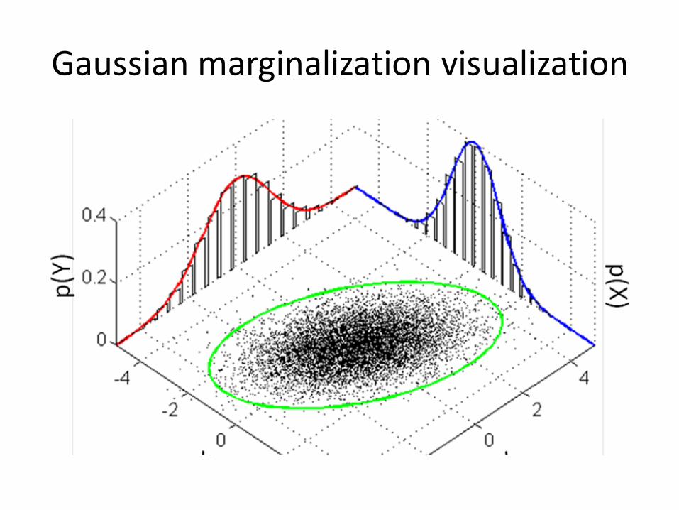
Gaussianmarginalizationvisualization
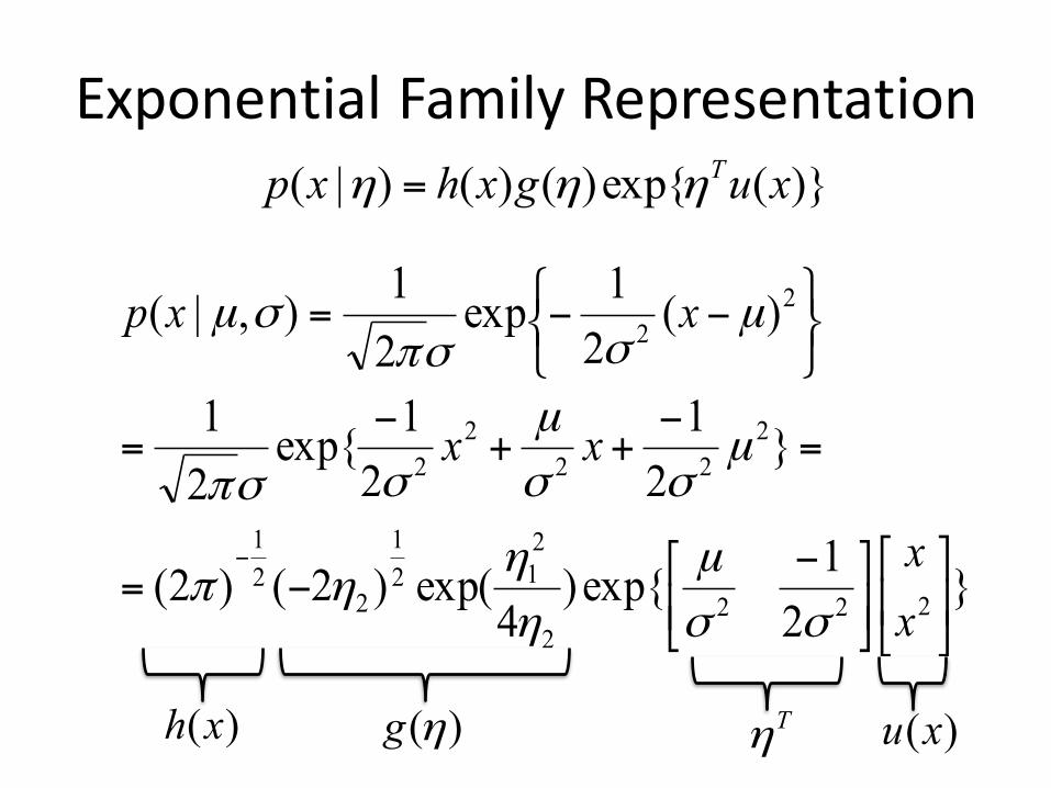
ExponentialFamilyRepresentation
}21exp{)
4exp()2()2(
}21
21exp{
21
)(21exp
21),|(
2222
212
1
221
222
22
22
⎥⎦
⎤⎢⎣
⎡⎥⎦
⎤⎢⎣
⎡ −−=
=−
++−
=
⎭⎬⎫
⎩⎨⎧ −−=
−
xx
xx
xxp
σσµ
ηη
ηπ
µσσ
µσσπ
µσσπ
σµ
)}(exp{)()()|( xugxhxp Tηηη =
)(xh )(ηg Tη )(xu
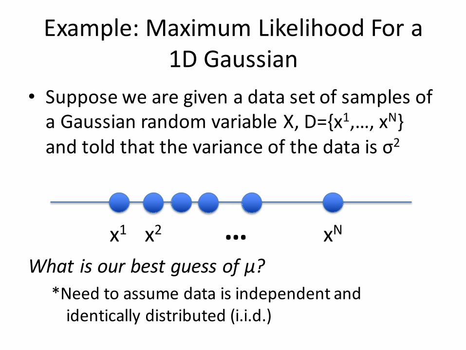
Example:MaximumLikelihoodFora1DGaussian
• SupposewearegivenadatasetofsamplesofaGaussianrandomvariableX,D={x1,…,xN}andtoldthatthevarianceofthedataisσ2
Whatisourbestguessofµ?*Needtoassumedataisindependentandidenticallydistributed(i.i.d.)
x1 x2 xN…
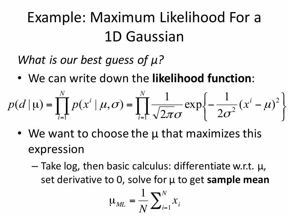
Example:MaximumLikelihoodFora1DGaussian
Whatisourbestguessofµ?• Wecanwritedownthelikelihoodfunction:
• Wewanttochoosetheµthatmaximizesthisexpression– Takelog,thenbasiccalculus:differentiatew.r.t.µ,setderivativeto0,solveforµtogetsamplemean
∏ ∏= = ⎭
⎬⎫
⎩⎨⎧ −−==µ
N
i
N
i
ii xxpdp1 1
22 )(
21exp
21),|()|( µ
σσπσµ
€
µML =1N
xii=1
N∑
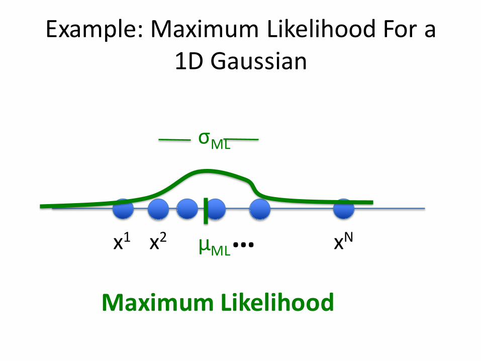
Example:MaximumLikelihoodFora1DGaussian
x1 x2 xN…µML
σML
MaximumLikelihood
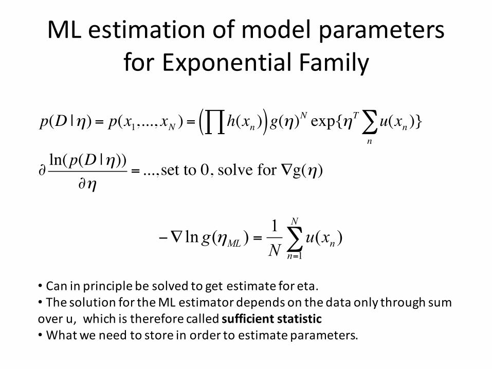
MLestimationofmodelparametersforExponentialFamily
p(D |η) = p(x1,..., xN ) = h(xn )∏( )g(η)N exp{ηT u(xnn∑ )}
∂ln(p(D |η))
∂η= ..., set to 0, solve for ∇g(η)
∑=
=∇−N
nnML xu
Ng
1)(1)(ln η
• Caninprinciplebesolvedtogetestimateforeta.• ThesolutionfortheMLestimatordependsonthedataonlythroughsumoveru,whichisthereforecalledsufficientstatistic•Whatweneedtostoreinordertoestimateparameters.
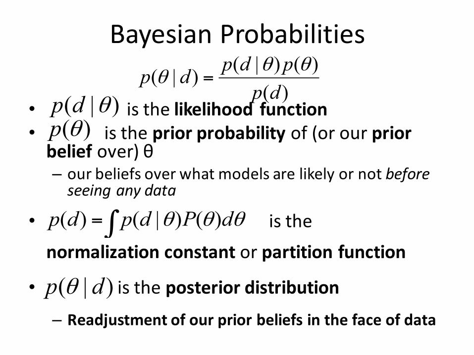
BayesianProbabilities
• isthelikelihood function• isthepriorprobability of(orourpriorbelief over)θ– ourbeliefsoverwhatmodelsarelikelyornotbeforeseeinganydata
• isthenormalizationconstantorpartitionfunction
• istheposteriordistribution
– Readjustmentofourpriorbeliefsinthefaceofdata
)()()|()|(
dppdpdp θθ
θ =
∫= θθθ dPdpdp )()|()(
)|( θdp)(θp
)|( dp θ
Example:BayesianInferenceFora1DGaussian
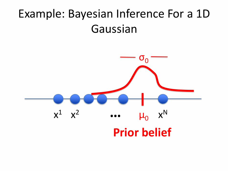
• SupposewehaveapriorbeliefthatthemeanofsomerandomvariableXisµ0 andthevarianceofourbeliefisσ02
• WearethengivenadatasetofsamplesofX,d={x1,…,xN}andsomehowknowthatthevarianceofthedataisσ2
Whatistheposteriordistributionover(ourbeliefaboutthevalueof)µ?
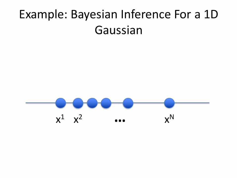
Example:BayesianInferenceFora1DGaussian
x1 x2 xN…

Example:BayesianInferenceFora1DGaussian
x1 x2 xN… µ0
σ0
Priorbelief
Example:BayesianInferenceFora1DGaussian
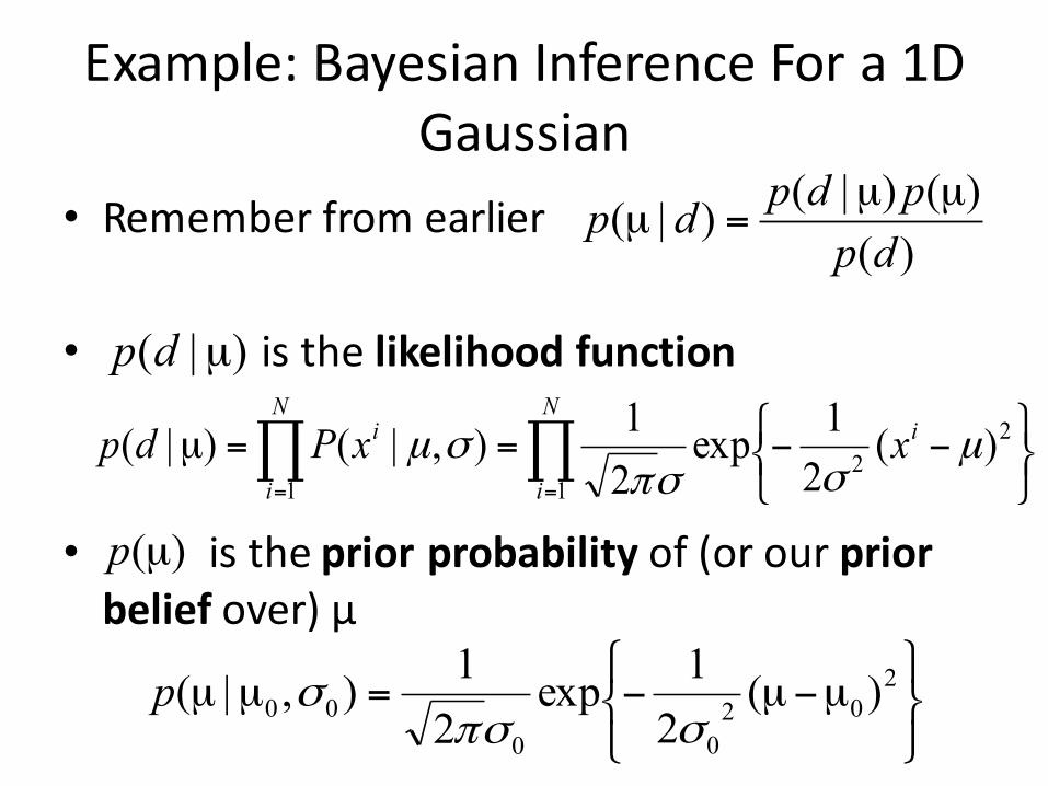
• Rememberfromearlier
• isthelikelihoodfunction
• isthepriorprobability of(orourpriorbelief over)µ
)()()|()|(
dppdpdp µµ
=µ
)|( µdp
)(µp
∏ ∏= = ⎭
⎬⎫
⎩⎨⎧ −−==µ
N
i
N
i
ii xxPdp1 1
22 )(
21exp
21),|()|( µ
σσπσµ
⎭⎬⎫
⎩⎨⎧
µ−µ−=µµ 202
0000 )(
21exp
21),|(
σσπσp
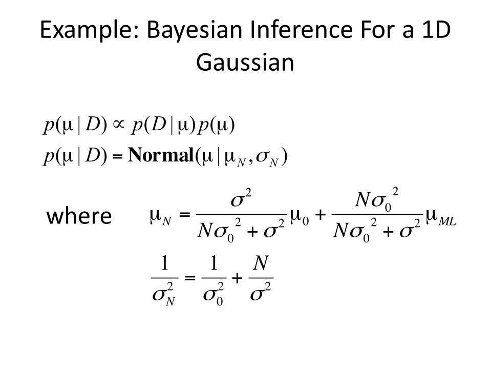
Example:BayesianInferenceFora1DGaussian
),|()|()()|()|(
NNDppDpDp
σµµ=µ
µµ∝µ
Normal
€
µN =σ 2
Nσ 02 +σ 2 µ0 +
Nσ 02
Nσ 02 +σ 2 µML
1σN2 =
1σ 02 +
Nσ 2
where
Example:BayesianInferenceFora1DGaussian
x1 x2 xN… µ0
σ0
Priorbelief
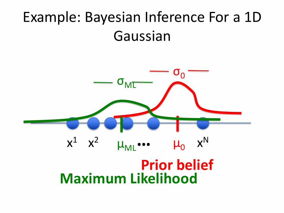
Example:BayesianInferenceFora1DGaussian
x1 x2 xN… µ0
σ0
PriorbeliefµML
σML
MaximumLikelihood
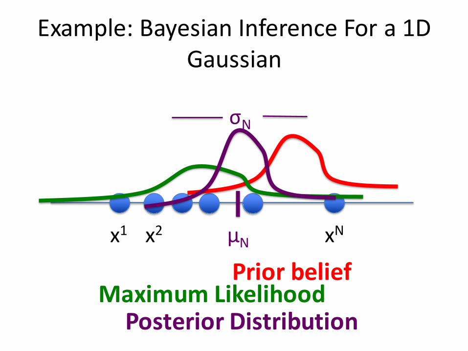
Example:BayesianInferenceFora1DGaussian
x1 x2 xNµN
σN
PriorbeliefMaximumLikelihood
PosteriorDistribution
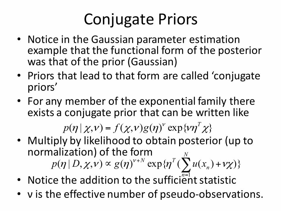
ConjugatePriors• NoticeintheGaussianparameterestimationexamplethatthefunctionalformoftheposteriorwasthatoftheprior(Gaussian)
• Priorsthatleadtothatformarecalled‘conjugatepriors’
• Foranymemberoftheexponentialfamilythereexistsaconjugatepriorthatcanbewrittenlike
• Multiplybylikelihoodtoobtainposterior(uptonormalization)oftheform
• Noticetheadditiontothesufficientstatistic• ν istheeffectivenumberofpseudo-observations.
}exp{)(),(),|( χνηηνχνχη ν Tgfp =
)})((exp{)(),,|(1
νχηηνχη ν +∝ ∑=
+N
nn
TN xugDp
ConjugatePriors- Examples
• BetaforBernoulli/binomial• Dirichlet forcategorical/multinomial• NormalformeanofNormal• Andmanymore...
• Whataresomepropertiesoftheconjugatepriorforthecovariance(orprecision)matrixofanormaldistribution?


