
Introduction to Image Processing
Grass
Sky
TreeTree
? ?
Edge Detection and Sharpening

Edge Detection and Sharpening
• The Basic Theory• Properties of 1st and 2nd Derivatives• Edge Detection
‒ gradient operators based on 1st derivatives‒ Laplacian as the 2nd derivative operator
• Edge Sharpening ‒ composite Laplacian − unsharp masking
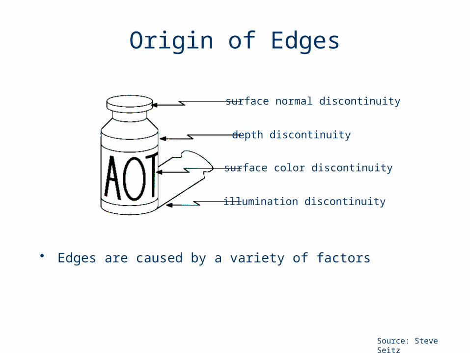
Origin of Edges
• Edges are caused by a variety of factors
depth discontinuity
surface color discontinuity
illumination discontinuity
surface normal discontinuity
Source: Steve Seitz

Edge Detection
• Edge is marked by points at which image properties change sharply
• To detect changes in a digital 2D image intensity function, f(x, y), a continuous image can be reconstructed, followed by the differentiation operator OR
• We take the discrete derivative (finite difference) shown below:

The Basic Theory
• An intensity jump (edge) generates a peak in the 1st derivative, and the peak generates a zero-crossing in the 2nd derivative (when the first derivative is at a maximum, the second derivative is zero)
• Gradient methods detect edges by looking for the maximum and minimum in the first derivative of the image
• Laplacian methods search for zero crossings in the second derivative of the image to find edges

• Sharpening filters are based on computing spatial derivatives of an image.
• The first-order derivative of a one-dimensional function f(x) is
• The second-order derivative of a one-dimensional function f(x) is
Alternative 1st and 2nd Derivatives

Properties of the 1st and 2nd Derivatives

Profile for 1st Derivative
Image Strip
0
1
2
3
4
5
6
7
8
1st Derivative
-8
-6
-4
-2
0
2
4
6
8
5 5 4 3 2 1 0 0 0 6 0 0 0 0 1 3 1 0 0 0 0 7 7 7 7
-1 -1 -1 -1 -1 0 0 6 -6 0 0 0 1 2 -2 -1 0 0 0 7 0 0 0

Profile for 2nd DerivativeImage Strip
0
1
2
3
4
5
6
7
8
5 5 4 3 2 1 0 0 0 6 0 0 0 0 1 3 1 0 0 0 0 7 7 7 7
2nd Derivative
-15
-10
-5
0
5
10
-1 0 0 0 0 1 0 6 -12 6 0 0 1 1 -4 1 1 0 0 7 -7 0 0
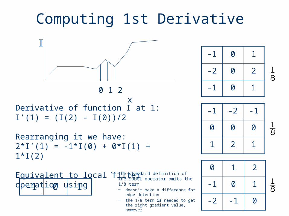
Computing 1st Derivative
I
0 1 2 x
Derivative of function I at 1:I’(1) = (I(2) - I(0))/2
Rearranging it we have:2*I’(1) = -1*I(0) + 0*I(1) + 1*I(2)
Equivalent to local filter operation using
-1 0 1
-1 0 1
-2 0 2
-1 0 1
-1 -2 -1
0 0 0
1 2 1
0 1 2
-1 0 1
-2 -1 0
• The standard definition of the Sobel operator omits the 1/8 term– doesn’t make a difference for edge
detection– the 1/8 term is needed to get the
right gradient value, however
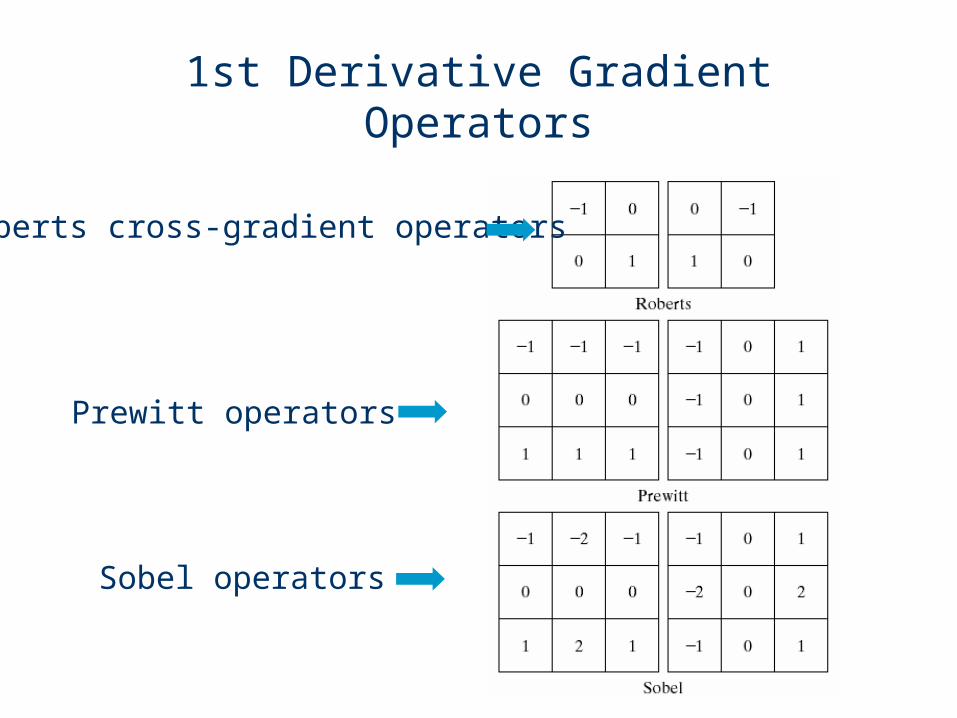
Roberts cross-gradient operators
Prewitt operators
Sobel operators
1st Derivative Gradient Operators

Prewitt masks for detecting diagonal edges
Sobel masks for detecting diagonal edges
1st Derivative Gradient Operators

• First-order derivatives:– The gradient of an image Gxy at location (x,y) is defined as
the vector:
– The gradient points in the direction of most rapid increase in intensity
– The edge strength is given by the gradient magnituge
O OR approx.
– The gradient direction is given by: How does this relate to the edge direction?
yfxf
y
x
G
Gf
Properties of Image Gradient
yx GGf

Gradients in 2D
• For an image function, I(x,y), the gradient direction, (x,y), gives the direction of steepest image gradient: (x,y) atan(Gy/Gx)
• This gives the direction of a line perpendicular to the edge
Gx
Gy
Gxy

Sobel Operator
Original Sobel

yx GGf
Gradient Operators: Examples

Gradient Operators: Examples

Gradient Operators: Examples

• Note that Prewitt operator is a box filter convolved with a derivative operator
• Also note a Sobel operator is a [1 2 1] filter convolved with a derivative operator
Important Observation

Computing 2nd Derivatives
I
0 1 2 x
I’’(1) = (I’(1.5) - I’(0.5))/1I’(0.5) = (I(1) - I(0))/1 and I’(1.5) = (I(2) - I(1))/1
\ I’’(1) = 1*I(0) – 2*I(1) + 1*I(2)
Equivalent to local filter operation with
1 -2 1
• The theory can be carried over to 2D as long as there is a way to approximate the derivative of a 2D image

• Development of the Laplacian method– The two dimensional Laplacian operator for continuous
functions:
– The Laplacian is a linear operator.
2
2
2
22
y
f
x
ff
),(2),1(),1(2
2
yxfyxfyxfx
f
),(2)1,()1,(2
2
yxfyxfyxfy
f
),(4)]1,()1,(),1(),1([2 yxfyxfyxfyxfyxff
Laplacian Operator

Laplacian Operator

• Applying the Laplacian to an image we get a new image that highlights edges and other discontinuities
OriginalImage
LaplacianFiltered Image
LaplacianFiltered Image
Scaled for Display
Laplacian Operator

But That Is Not Very Enhanced!
• The result of a Laplacian filtering is not an enhanced image
• We have to do more work in order to get our final image
• Subtract the Laplacian result from the original image to generate our final sharpened enhanced image
LaplacianFiltered Image
Scaled for Display
fyxfyxg 2),(),(

Laplacian Image Enhancement
In the final sharpened image edges and fine detail are much more obvious
- =
OriginalImage
LaplacianFiltered Image
SharpenedImage
positive. ismask Laplacian theoft coefficiencenter theif ),(
negative. ismask Laplacian theoft coefficiencenter theif ),(),(
2
2
fyxf
fyxfyxg

Simplified Image Enhancement
The entire enhancement can be combined into a single filtering operation
),1(),1([),( yxfyxfyxf )1,()1,( yxfyxf
)],(4 yxf
fyxfyxg 2),(),(
),1(),1(),(5 yxfyxfyxf )1,()1,( yxfyxf

Composite Laplacian Mask
• This gives us a new filter which does the whole job for us in one step
0 -1 0
-1 5 -1
0 -1 0

f2
Composite Laplacian Mask
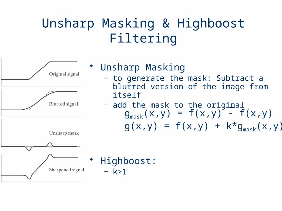
Unsharp Masking & Highboost Filtering
• Unsharp Masking‒ to generate the mask: Subtract a blurred
version of the image from itself ‒ add the mask to the original
• Highboost: ‒ k>1
gmask(x,y) = f(x,y) - f(x,y)g(x,y) = f(x,y) + k*gmask(x,y)

1st & 2nd DerivativesComparisons
• Observations:– 1st order derivatives generally produce thicker edges– 2nd order derivatives have a stronger response to fine detail
e.g. thin lines– 2nd order derivatives produce a double response at step
changes in grey level• The 2nd derivative is more useful for image enhancement
than the 1st derivative– Stronger response to fine detail– Simpler implementation– Because these kernels approximate a second derivative
measurement on the image, they are very sensitive to noise. To counter this, the image is often Gaussian smoothed before applying the Laplacian filter

Acknowlegements
Slides are modified based on the original slide set from Dr Li Bai, The University of Nottingham, Jubilee Campus plus the following sources:
• Digital Image Processing, by Gonzalez and Woods• http://www.comp.dit.ie/bmacnamee/materials/dip/lectures/
ImageProcessing6-SpatialFiltering2.ppt


