
INTRODUCTION TO T-TEST
Chapter 7

Hypothesis testing
• Critical region
• Region of rejection
• Defines “unlikely event” for H0
distribution
• Alpha ( )
• Probability value for critical region
• If set .05 = probability of result
occurred by chance only 5x out of 100
• Critical value (cv)
• Value of the statistic for alpha
• p-value
• Actual probability of result occurring

Review: z-test
• Hypothesis: Special training in reading skills will produce
change in scores.
• Reading skills for population: N(65, 15)
• Treatment group: N = 25; M = 70
• Is there evidence that training has an effect?
N
Mz

Review: z-test
• State hypotheses • H0: µ = 65
• H1: µ ≠ 65 (2-tailed)
• α = .05; so critical region = ?
• zcv = 1.96
• Calculate test statistic (z-test = ?)
• Make decision and state conclusion
• Fail to reject H0
• “No evidence that special training changed scores, z (n = 25) =
1.67, p = ns.”
67.1
25
15
6570
z
N
Mz
Review: z-test
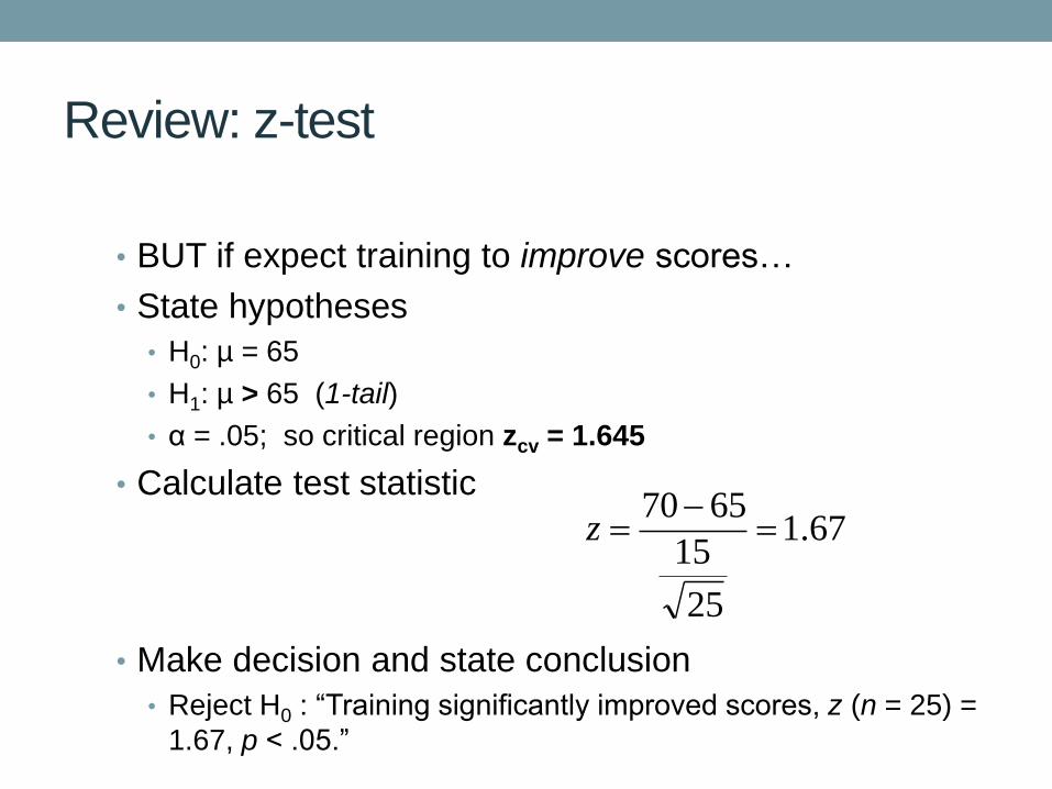
• BUT if expect training to improve scores…
• State hypotheses
• H0: µ = 65
• H1: µ > 65 (1-tail)
• α = .05; so critical region zcv = 1.645
• Calculate test statistic
• Make decision and state conclusion
• Reject H0 : “Training significantly improved scores, z (n = 25) =
1.67, p < .05.”
67.1
25
15
6570
z

Errors
Type I
error
Correct
decision
Correct
decision
Type II
error
Actual situation
NO Effect Effect
H0 True H0 False
Reject H0
Retain H0
Experimenter’s
Decision
Conclude there was
an effect when there
actually wasn’t – the
risk of that is
Conclude there wasn’t
an effect when there
actually was an effect –
also called

Type I and Type II errors
• Type I: Incorrectly conclude significant difference • Conclude treatment has an effect but really doesn’t
• Type II: Miss a significant result • Conclude no effect of treatment when it really does
• Which is worse error to make?
• Examples: • Law:
• Type I: Jury says guilty when innocent
• Type II: Jury says innocent when guilty
• Medicine:
• Type I: Doctor says cancer present when isn’t
• Type II: Doctor says no cancer when it is there
• Answer: it depends!

Setting your alpha level
• Lower alpha to
minimize chance of
Type I error
• But, then increase
chance of Type II
error!

Concerns with Alpha
• All-or-none decision
• Reject or accept null hypothesis
• Alpha (criteria) is set arbitrarily
• Null hypothesis logic is artificial
• No such thing as “no effect”
• Doesn’t give size of effect
• p-value is chance of occurrence
• Cannot say “very significant”!
• Sample size changes p-value (probability of rejecting H0)

Statistical Power
• What is the probability of making the correct decision??
• If treatment effect truly exists either…
• We correctly detect the effect or…
• We fail to detect the effect (Type II error or )
• So, the probability of correctly detecting is 1 -
• Power: probability that test will correctly reject null hypothesis
(i.e. will detect effect)
• Power depends on:
• Size of effect
• Alpha level
• Sample size
-3 -2 -1 0 1 2 3-3 -2 -1 0 1 2 3
Reject H0

Small
effect size
Large
effect size

Large
sample
size ->
small SD
Small
sample
size ->
large SD

Concerns with z-test
• Assumptions
• Must have a normal distribution
• Must know population mean and deviation
• Population mean (µ)
• Population standard deviation (σ)
• If don’t know above info or can’t make
assumptions need to use other statistics!
• Use “statistics” to make inferences
• Inferential statistics test: t-test

T-test: Estimates
• We’ve been using the z-score or z-test
formulas…
• Where M = standard error of the mean
• Instead…
• Use t-test
• Where M is a sample mean
• Where µ can be the population mean or
hypothetical H0 mean (i.e. chance or 0)
• Where sM = estimated standard error
N
MZ
M
MZ
XZ
OR
n
s2
n
s
Ms
Mt
OR

From z to t
• We use the “one-sample t-test” when we don’t
know .
• Use the sample variance instead of population SD
parameter ( )
• And, use hypothesized µ from the H0
n
Mz
n
s
Mt
2
N
s
Mt
OR

t-distribution
• “Student’s t-distribution”
similar in shape to N(0,1)
• Symmetric around 0
• Spread of t is greater
than N(0,1)
• As N increases, curve
approaches N(0,1)
• Different distributions
for “df” or n -1
• “Degrees of freedom”
• Table A.3 pp384

t table
• Is the t* (tcv) at
or higher than t
(statistic) given
df and α level
selected?

Finding the Critical t*
• Find the df in the left column
• Go across top to find the selected a level.
• Find the critical value, t*, for the df and a.
• If the absolute value of t is greater than or equal to t* then the test is significant at the a level.
• *Not all df are provided, so use the smaller df
(larger t*) for a more conservative estimate.

Eating behaviors
• “ATE”: positive attitude toward eating scale
• 3-point scale: -1 neg, 0 neutral, +1 positive
• 5 items: Eating desserts, snacks, etc.
• Minimum: -5; Maximum: +5
• Null hypothesis
• ATE = 0
• Alternative hypothesis
• ATE ≠ 0
• What values are needed to calculate the t-test?
• N
• Sample M and SD

t-test:
• N = 40 women
• ATE results: M = 0.525, SD = 2.16
• H0: ATE = 0
• Calculate t-test:
• 1.5?? Look up in t-table tcv
• Not every df so use df = 30:
• tcv = 2.042 = p = .05, 2-tailed
• Does not exceed critical value, so not significant
• Reporting a t-statistic: t(df) = value, p = value
• Women were found to have a neutral feeling toward eating, t(39) = 1.5, p = ns.
Ms
Mt
5.135.0
525.0
40
16.2
0525.0
t

Eating behaviors
• Women rated their feelings toward eating on a 3-point
scale.
• Participants’ average response (M = 0.5, SD = 2.16)
was not found to be significantly different from a neutral
rating of zero, t(39) = 1.5, p = ns.
• The results suggest that women do not have an overly
positive or negative feeling toward eating.

Confidence intervals
• CI: % confident that interval contains population
mean (µ)
• % is determined by researcher (e.g. 85, 90, 95%)
• Formula for z-test and t-test:
• CI = M +/- z*(σM)
• CI = M +/- t*(sM)
• Where z* or t* is the critical value
• Example:
• CI = 86 +/- 1.96(1.7) = 82.67 to 89.33
• 95% confident pop mean in this range

Spatial map study

Spatial Map Study
• % correct: academic, athletic, residence halls, social, administrative,
parking locations on campus
• H0 = 50% correct, H1 > 50% correct (1-tailed)
• Information: N = 11, M = 0.36, SD = 0.15
• df 10; for α=.05 (1 tail): t* or tcv= 1.812
(tcv = 3.169 for p = .0005 (1tail))
Participants remembered significantly less than 50% of the campus
map (M = .36), t(10) = -3.11, p < .01.
CI = M +/- t*(sM) = 0.36 +/- 1.812 (.045) = 0.68 to 0.28
95% confident that true mean falls within that range
N
s
Mt
045.
14.0
11
15.
50.36.
t t = -3.11

Lateralization in Perception of Emotion
• Two chimeric faces – which one is
happier (or younger example)?
• Emotion is processed in the right
hemisphere
• Dependent variable:
• Total score: -36 to +36
• where 0 = no lateralization
• What are the hypotheses?
• Null hypothesis: Total score = 0
• Alternative hypothesis?
Total score ≠ 0

t-test example
• Lateralization study (N = 173)
• H0: totscore = 0
• Totscore M = -11.7, SD = 16.6, S2 = 276
• t-test: -11.7 – 0 = -11.7 = - 9.28
sqrt(276/173) 1.26
• -9.28?? Look up tcv in table…
• Use 120: tcv = 2.576 = p = .005
• Participants show a significant lateralization to detect emotion using the right hemisphere, t(172) = 9.28, p < .005
• CI = M +/- t*(sM) = -11.7 +/- 2.576 (1.26) = -8.45 to -14.95

Lateralization results
• Participants demonstrated a statistically
significant lateralization effect, t(172) = -9.28,
p < .05. Emotion was more influenced by the
right hemisphere (M = -11.7, CI (.95) = -8.45
to -14.95), as opposed to what would be
expected by chance (M = 0).


