Invertible Residual Networks

Jens Behrmann * 1 2 Will Grathwohl * 2 Ricky T. Q. Chen 2 David Duvenaud 2 Jorn-Henrik Jacobsen * 2

AbstractWe show that standard ResNet architectures canbe made invertible, allowing the same model tobe used for classification, density estimation, andgeneration. Typically, enforcing invertibility re-quires partitioning dimensions or restricting net-work architectures. In contrast, our approach onlyrequires adding a simple normalization step dur-ing training, already available in standard frame-works. Invertible ResNets define a generativemodel which can be trained by maximum like-lihood on unlabeled data. To compute likeli-hoods, we introduce a tractable approximation tothe Jacobian log-determinant of a residual block.Our empirical evaluation shows that invertibleResNets perform competitively with both state-of-the-art image classifiers and flow-based gener-ative models, something that has not been previ-ously achieved with a single architecture.

1. IntroductionOne of the main appeals of neural network-based models isthat a single model architecture can often be used to solvea variety of related tasks. However, many recent advancesare based on special-purpose solutions tailored to particu-lar domains. State-of-the-art architectures in unsupervisedlearning, for instance, are becoming increasingly domain-specific (Van Den Oord et al., 2016b; Kingma & Dhariwal,2018; Parmar et al., 2018; Karras et al., 2018; Van Den Oordet al., 2016a). On the other hand, one of the most success-ful feed-forward architectures for discriminative learningare deep residual networks (He et al., 2016; Zagoruyko &Komodakis, 2016), which differ considerably from theirgenerative counterparts. This divide makes it complicatedto choose or design a suitable architecture for a given task.It also makes it hard for discriminative tasks to benefit from

*Equal contribution 1University of Bremen, Center for Indus-trial Mathematics 2Vector Institute and University of Toronto. Cor-respondence to: Jens Behrmann <jensb@uni-bremen.de>, Jorn-Henrik Jacobsen <j.jacobsen@vectorinstitute.ai>.

Proceedings of the 36 th International Conference on MachineLearning, Long Beach, California, PMLR 97, 2019. Copyright2019 by the author(s).

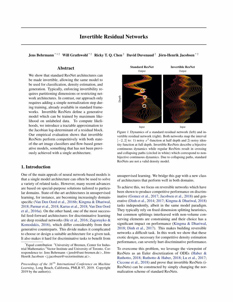
OutputStandard ResNet

OutputInvertible ResNet

InputInput

Depth

Figure 1. Dynamics of a standard residual network (left) and in-vertible residual network (right). Both networks map the interval[−2, 2] to: 1) noisy x3-function at half depth and 2) noisy iden-tity function at full depth. Invertible ResNets describe a bijectivecontinuous dynamics while regular ResNets result in crossingand collapsing paths (circled in white) which correspond to non-bijective continuous dynamics. Due to collapsing paths, standardResNets are not a valid density model.

unsupervised learning. We bridge this gap with a new classof architectures that perform well in both domains.

To achieve this, we focus on reversible networks which havebeen shown to produce competitive performance on discrim-inative (Gomez et al., 2017; Jacobsen et al., 2018) and gen-erative (Dinh et al., 2014; 2017; Kingma & Dhariwal, 2018)tasks independently, albeit in the same model paradigm.They typically rely on fixed dimension splitting heuristics,but common splittings interleaved with non-volume con-serving elements are constraining and their choice has asignificant impact on performance (Kingma & Dhariwal,2018; Dinh et al., 2017). This makes building reversiblenetworks a difficult task. In this work we show that theseexotic designs, necessary for competitive density estimationperformance, can severely hurt discriminative performance.

To overcome this problem, we leverage the viewpoint ofResNets as an Euler discretization of ODEs (Haber &Ruthotto, 2018; Ruthotto & Haber, 2018; Lu et al., 2017;Ciccone et al., 2018) and prove that invertible ResNets (i-ResNets) can be constructed by simply changing the nor-malization scheme of standard ResNets.

Invertible Residual Networks

As an intuition, Figure 1 visualizes the differences in thedynamics learned by standard and invertible ResNets.

This approach allows unconstrained architectures for eachresidual block, while only requiring a Lipschitz constantsmaller than one for each block. We demonstrate that thisrestriction negligibly impacts performance when buildingimage classifiers - they perform on par with their non-invertible counterparts on classifying MNIST, CIFAR10and CIFAR100 images.

We then show how i-ResNets can be trained as maximumlikelihood generative models on unlabeled data. To com-pute likelihoods, we introduce a tractable approximationto the Jacobian determinant of a residual block. LikeFFJORD (Grathwohl et al., 2019), i-ResNet flows haveunconstrained (free-form) Jacobians, allowing them to learnmore expressive transformations than the triangular map-pings used in other reversible models. Our empirical evalua-tion shows that i-ResNets perform competitively with bothstate-of-the-art image classifiers and flow-based generativemodels, bringing general-purpose architectures one stepcloser to reality.1

2. Enforcing Invertibility in ResNetsThere is a remarkable similarity between ResNet architec-tures and Euler’s method for ODE initial value problems:

xt+1 ← xt + gθt(xt)

xt+1 ← xt + hfθt(xt)

where xt ∈ Rd represent activations or states, t representslayer indices or time, h > 0 is a step size, and gθt is aresidual block. This connection has attracted research at theintersection of deep learning and dynamical systems (Luet al., 2017; Haber & Ruthotto, 2018; Ruthotto & Haber,2018; Chen et al., 2018). However, little attention has beenpaid to the dynamics backwards in time

xt ← xt+1 − gθt(xt)xt ← xt+1 − hfθt(xt)

which amounts to the implicit backward Euler discretization.In particular, solving the dynamics backwards in time wouldimplement an inverse of the corresponding ResNet. Thefollowing theorem states that a simple condition suffices tomake the dynamics solvable and thus renders the ResNetinvertible:

Theorem 1 (Sufficient condition for invertible ResNets).Let Fθ : Rd → Rd with Fθ = (F 1

θ ◦ . . . ◦ FTθ ) denote aResNet with blocks F tθ = I + gθt . Then, the ResNet Fθ is

1Official code release: https://github.com/jhjacobsen/invertible-resnet

Algorithm 1. Inverse of i-ResNet layer via fixed-point iteration.Input: output from residual layer y, contractive residualblock g, number of fixed-point iterations nInit: x0 := yfor i = 0, . . . , n doxi+1 := y − g(xi)

end for

invertible if

Lip(gθt) < 1, for all t = 1, . . . , T,

where Lip(gθt) is the Lipschitz-constant of gθt .

Note that this condition is not necessary for invertibility.Other approaches (Dinh et al., 2014; 2017; Jacobsen et al.,2018; Chang et al., 2018; Kingma & Dhariwal, 2018) relyon partitioning dimensions or autoregressive structures tocreate analytical inverses.

While enforcing Lip(g) < 1 makes the ResNet invertible,we have no analytic form of this inverse. However, wecan obtain it through a simple fixed-point iteration, seeAlgorithm 1. Note, that the starting value for the fixed-pointiteration can be any vector, because the fixed-point is unique.However, using the output y = x+g(x) as the initializationx0 := y is a good starting point since y was obtained fromx only via a bounded perturbation of the identity. From theBanach fixed-point theorem we have

‖x− xn‖2 ≤Lip(g)n

1− Lip(g)‖x1 − x0‖2. (1)

Thus, the convergence rate is exponential in the number ofiterations n and smaller Lipschitz constants will yield fasterconvergence.

Additional to invertibility, a contractive residual block alsorenders the residual layer bi-Lipschitz.

Lemma 2 (Lipschitz constants of Forward and Inverse). LetF (x) = x+ g(x) with Lip(g) = L < 1 denote the residuallayer. Then, it holds

Lip(F ) ≤ 1 + L and Lip(F−1) ≤ 1

1− L.

Hence by design, invertible ResNets offer stability guar-antees for both their forward and inverse mapping. In thefollowing section, we discuss approaches to enforce theLipschitz condition.

2.1. Satisfying the Lipschitz Constraint

We implement residual blocks as a composition of contrac-tive nonlinearities φ (e.g. ReLU, ELU, tanh) and linearmappings.

Invertible Residual Networks

For example, in our convolutional networks g =W3φ(W2φ(W1)), where Wi are convolutional layers.Hence,

Lip(g) < 1, if ‖Wi‖2 < 1,

where ‖ · ‖2 denotes the spectral norm. Note, that regular-izing the spectral norm of the Jacobian of g (Sokoli et al.,2017) only reduces it locally and does not guarantee theabove condition. Thus, we will enforce ‖Wi‖2 < 1 for eachlayer.

A power-iteration on the parameter matrix as in Miyato et al.(2018) approximates only a bound on ‖Wi‖2 instead of thetrue spectral norm, if the filter kernel is larger than 1 × 1,see Tsuzuku et al. (2018) for details on the bound. Hence,unlike Miyato et al. (2018), we directly estimate the spectralnorm of Wi by performing power-iteration using Wi andWTi as proposed in Gouk et al. (2018). The power-iteration

yields an under-estimate σi ≤ ‖Wi‖2. Using this estimate,we normalize via

Wi =

{cWi/σi, if c/σi < 1

Wi, else, (2)

where the hyper-parameter c < 1 is a scaling coefficient.Since σi is an under-estimate, ‖Wi‖2 ≤ c is not guaran-teed. However, after training Sedghi et al. (2019) offer anapproach to inspect ‖Wi‖2 exactly using the SVD on theFourier transformed parameter matrix, which will allow usto show Lip(g) < 1 holds in all cases.

3. Generative Modelling with i-ResNetsWe can define a simple generative model for data x ∈ Rdby first sampling z ∼ pz(z) where z ∈ Rd and then defin-ing x = Φ(z) for some function Φ : Rd → Rd. If Φ isinvertible and we define F = Φ−1, then we can computethe likelihood of any x under this model using the changeof variables formula

ln px(x) = ln pz(z) + ln |det JF (x)|, (3)

where JF (x) is the Jacobian of F evaluated at x. Modelsof this form are known as Normalizing Flows (Rezende &Mohamed, 2015). They have recently become a popularmodel for high-dimensional data due to the introduction ofpowerful bijective function approximators whose Jacobianlog-determinant can be efficienty computed (Dinh et al.,2014; 2017; Kingma & Dhariwal, 2018; Chen et al., 2018)or approximated (Grathwohl et al., 2019).

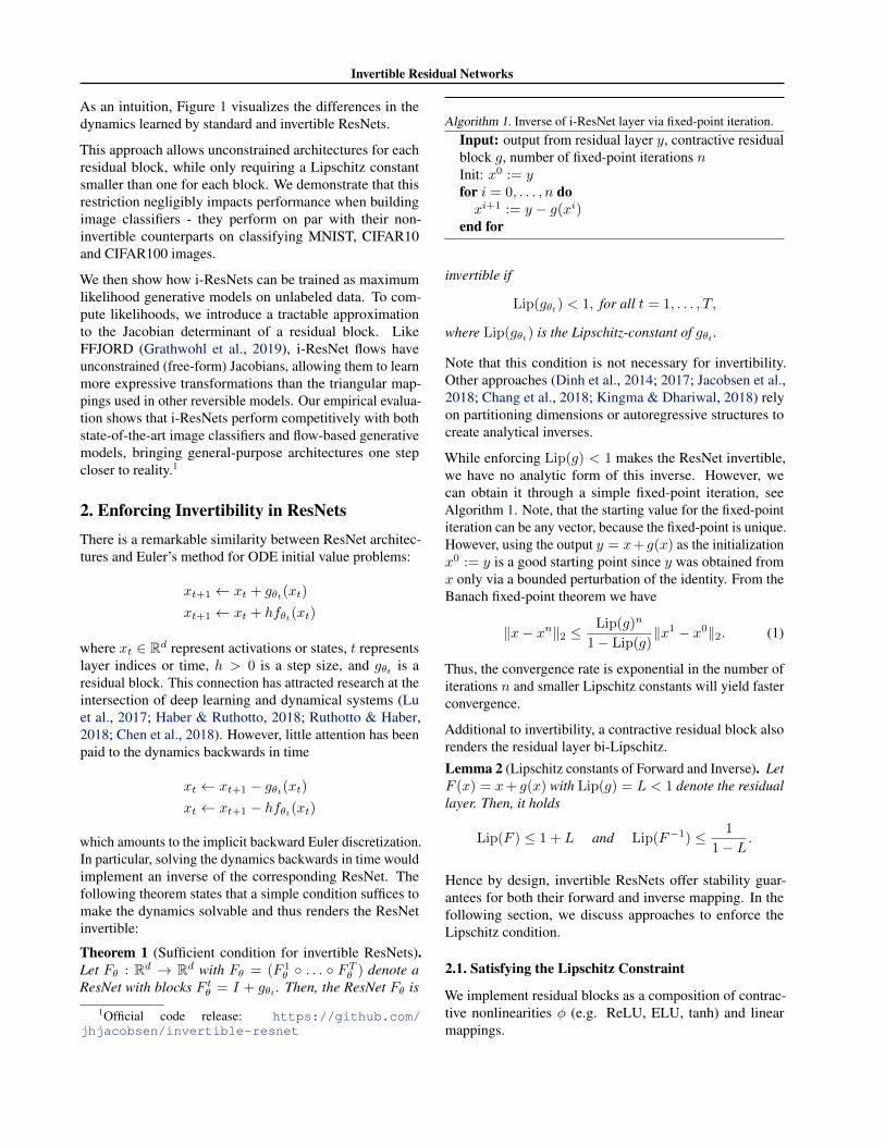
Since i-ResNets are guaranteed to be invertible we can usethem to parameterize F in Equation (3). Samples from thismodel can be drawn by first sampling z ∼ p(z) and thencomputing x = F−1(z) with Algorithm 1. In Figure 2 we

Data Samples Glow i-ResNet

Figure 2. Visual comparison of i-ResNet flow and Glow. Detailsof this experiment can be found in Appendix C.3.

show an example of using an i-ResNet to define a genera-tive model on some two-dimensional datasets compared toGlow (Kingma & Dhariwal, 2018).

3.1. Scaling to Higher Dimensions

While the invertibility of i-ResNets allows us to usethem to define a Normalizing Flow, we must computeln |det JF (x)| to evaluate the data-density under the model.Computing this quantity has a time cost of O(d3) in gen-eral which makes naıvely scaling to high-dimensional dataimpossible.

To bypass this constraint we present a tractable approxima-tion to the log-determinant term in Equation (3), which willscale to high dimensions d. Previously, Ramesh & LeCun(2018) introduced the application of log-determinant estima-tion to non-invertible deep generative models without thespecific structure of i-ResNets.

First, we note that the Lipschitz constrained perturbationsx+ g(x) of the identity yield positive determinants, hence

|det JF (x)| = det JF (x),

see Lemma 6 in Appendix A. Combining this result withthe matrix identity ln det(A) = tr(ln(A)) for non-singularA ∈ Rd×d (see e.g. Withers & Nadarajah (2010)), we have

ln |det JF (x)| = tr(ln JF ),

where tr denotes the matrix trace and ln the matrix loga-rithm. Thus for z = F (x) = (I + g)(x), it is

ln px(x) = ln pz(z) + tr(ln(I + Jg(x)

)).

The trace of the matrix logarithm can be expressed as a

Invertible Residual Networks

power series (Hall, 2015)

tr(ln(I + Jg(x)

))=

∞∑k=1

(−1)k+1tr(Jkg)

k, (4)

which converges if ‖Jg‖2 < 1. Hence, due to the Lipschitzconstraint, we can compute the log-determinant via theabove power series with guaranteed convergence.

Before we present a stochastic approximation to the abovepower series, we observe following properties of i-ResNets:Due to Lip(gt) < 1 for the residual block of each layer t, wecan provide a lower and upper bound on its log-determinantwith

d

T∑t=1

ln(1− Lip(gt)) ≤ ln |det JF (x)|

d

T∑t=1

ln(1 + Lip(gt)) ≥ ln |det JF (x)|,

for all x ∈ R, see Lemma 7 in Appendix A. Thus, both thenumber of layers T and the Lipschitz constant affect thecontraction and expansion bounds of i-ResNets and must betaken into account when designing such an architecture.

3.2. Stochastic Approximation of log-determinant

Expressing the log-determinant with the power series in(4) has three main computational drawbacks: 1) Comput-ing tr(Jg) exactly costs O(d2), or approximately needs devaluations of g as each entry of the diagonal of the Jaco-bian requires the computation of a separate derivative of g(Grathwohl et al., 2019). 2) Matrix powers Jkg are needed,which requires the knowledge of the full Jacobian. 3) Theseries is infinite.

Fortunately, drawback 1) and 2) can be alleviated. First,vector-Jacobian products vTJg can be computed at approxi-mately the same costs as evaluating g through reverse-modeautomatic differentiation. Second, a stochastic approxima-tion of the matrix trace of A ∈ Rd×d

tr(A) = Ep(v)[vTAv

],

known as the Hutchinsons trace estimator, can be usedto estimate tr

(Jkg). The distribution p(v) needs to fulfill

E[v] = 0 and Cov(v) = I , see (Hutchinson, 1990; Avron &Toledo, 2011).

While this allows for an unbiased estimate of the matrixtrace, to achieve bounded computational costs, the powerseries (4) will be truncated at index n to address drawback3). Algorithm 2 summarizes the basic steps. The truncationturns the unbiased estimator into a biased estimator, wherethe bias depends on the truncation error. Fortunately, thiserror can be bounded as we demonstrate below.

Algorithm 2. Forward pass of an invertible ResNets with Lipschitzconstraint and log-determinant approximation, SN denotes spectralnormalization based on (2).

Input: data point x, network F , residual block g, numberof power series terms nfor Each residual block do

Lip constraint: Wj := SN(Wj , x) for linear Layer Wj .Draw v from N (0, I)wT := vT

ln det := 0for k = 1 to n dowT := wT Jg (vector-Jacobian product)ln det := ln det +(−1)k+1wT v/k

end forend for

To improve the stability of optimization when using this es-timator we recommend using nonlinearities with continuousderivatives such as ELU (Clevert et al., 2015) or softplusinstead of ReLU (See Appendix C.3).

3.3. Error of Power Series Truncation

We estimate ln |det(I + Jg)| with the finite power series

PS(Jg, n) :=

n∑k=1

(−1)k+1tr(Jkg)

k, (5)

where we have (with some abuse of notation) PS(Jg,∞) =tr(ln(I + Jg)). We are interested in bounding the trunca-tion error of the log-determinant as a function of the datadimension d, the Lipschitz constant Lip(g) and the numberof terms in the series n.Theorem 3 (Approximation error of Loss). Let g denotethe residual function and Jg the Jacobian as before. Then,the error of a truncated power series at term n is boundedas

|PS(Jg, n)− ln det(I + Jg)|

≤ − d

(ln(1− Lip(g)) +

n∑k=1

Lip(g)k

k

).

While the result above gives an error bound for evaluation ofthe loss, during training the error in the gradient of the lossis of greater interest. Similarly, we can obtain the followingbound. The proofs are given in Appendix A.Theorem 4 (Convergence Rate of Gradient Approximation).Let θ ∈ Rp denote the parameters of network F , let g, Jgbe as before. Further, assume bounded inputs and a Lips-chitz activation function with Lipschitz derivative. Then, weobtain the convergence rate

‖∇θ(ln det

(I + Jg

))− PS

(Jg, n

))‖∞ = O(cn)

Invertible Residual Networks

where c := Lip(g) and n the number of terms used in thepower series.

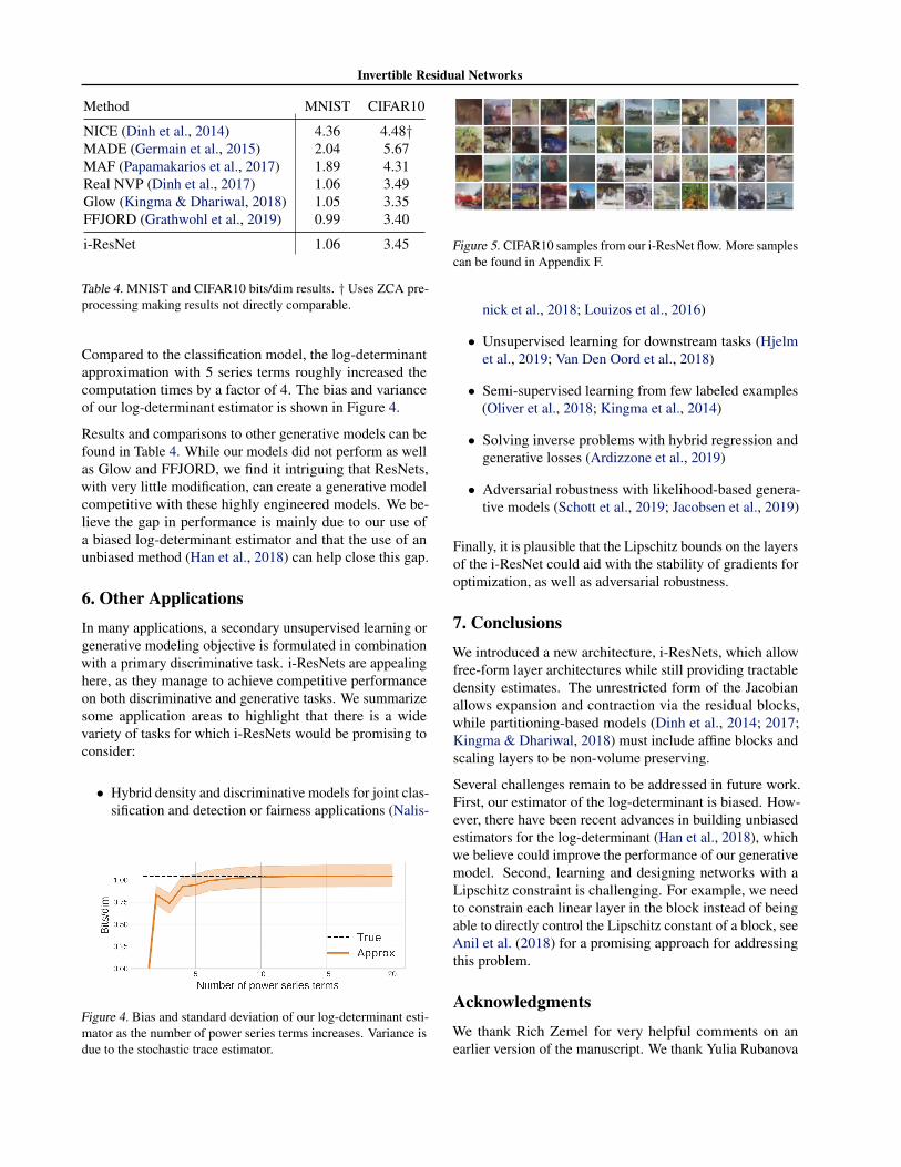
In practice, only 5-10 terms must be taken to obtain a biasless than .001 bits per dimension, which is typically reportedup to .01 precision (See Appendix E).

4. Related Work4.1. Reversible Architectures

We put our focus on invertible architectures with efficientinverse computation, namely NICE (Dinh et al., 2014), i-RevNet (Jacobsen et al., 2018), Real-NVP (Dinh et al.,2017), Glow (Kingma & Dhariwal, 2018) and NeuralODEs (Chen et al., 2018) and its stochastic density esti-mator FFJORD (Grathwohl et al., 2019). A summary of thecomparison between different reversible networks is givenin Table 1.

The dimension-splitting approach used in NICE, i-RevNet,Real-NVP and Glow allows for both analytic forward andinverse mappings. However, this restriction required theintroduction of additional steps like invertible 1 × 1 convo-lutions in Glow (Kingma & Dhariwal, 2018). These 1 × 1convolutions need to be inverted numerically, making Glowaltogether not analytically invertible. In contrast, i-ResNetcan be viewed as an intermediate approach, where the for-ward mapping is given analytically, while the inverse can becomputed via a fixed-point iteration.

Furthermore, an i-ResNet block has a Lipschitz bound bothfor forward and inverse (Lemma 2), while other approachesdo not have this property by design. Hence, i-ResNets couldbe an interesting avenue for stability-critical applicationslike inverse problems (Ardizzone et al., 2019) or invariance-based adversarial vulnerability (Jacobsen et al., 2019).

Neural ODEs (Chen et al., 2018) allow free-form dynamicssimilar to i-ResNets, meaning that any architecture could beused as long as the input and output dimensions are the same.To obtain discrete forward and inverse dynamics, NeuralODEs rely on adaptive ODE solvers, which allows for anaccuracy vs. speed trade-off. Yet, scalability to very highinput dimension such as high-resolution images remainsunclear.

4.2. Ordinary Differential Equations

Due to the similarity of ResNets and Euler discretizations,there are many connections between the i-ResNet and ODEs,which we review in this section.

Relationship of i-ResNets to Neural ODEs: The view ofdeep networks as dynamics over time offers two fundamen-tal learning approaches: 1) Direct learning of dynamicsusing discrete architectures like ResNets (Haber & Ruthotto,

2018; Ruthotto & Haber, 2018; Lu et al., 2017; Cicconeet al., 2018). 2) Indirect learning of dynamics via parametriz-ing an ODE with a neural network as in Chen et al. (2018);Grathwohl et al. (2019).

The dynamics x(t) of a fixed ResNet Fθ are only defined attime points ti corresponding to each block gθti . However, alinear interpolation in time can be used to generate continu-ous dynamics. See Figure 1, where the continuous dynam-ics of a linearly interpolated invertible ResNet are shownagainst those of a standard ResNet. Invertible ResNets arebijective along the continuous path while regular ResNetsmay result in crossing or merging paths. The indirect ap-proach of learning an ODE, on the other hand, adapts thediscretization based on an ODE-solver, but does not have afixed computational budget compared to an i-ResNet.

Stability of ODEs: There are two main approaches to studythe stability of ODEs, 1) behavior for t → ∞ and 2) Lip-schitz stability over finite time intervals [0, T ]. Based ontime-invariant dynamics f(x(t)), (Ciccone et al., 2018) con-structed asymptotically stable ResNets using anti-symmetriclayers such that Re(λ(Jx)) < 0 (with Re(λ(·)) denotingthe real-part of eigenvalues, ρ(·) spectral radius and Jxg theJacobian at point x). By projecting weights based on the Ger-shgorin circle theorem, they further fulfilled ρ(Jxg) < 1,yielding asymptotically stable ResNets with shared weightsover layers. On the other hand, (Haber & Ruthotto, 2018;Ruthotto & Haber, 2018) considered time-dependent dy-namics f(x(t), θ(t)) corresponding to standard ResNets.They induce stability by using anti-symmetric layers andprojections of the weights. Contrarily, initial value prob-lems on [0, T ] are well-posed for Lipschitz continuous dy-namics (Ascher, 2008). Thus, the invertible ResNet withLip(f) < 1 can be understood as a stabilizer of an ODEfor step size h = 1 without a restriction to anti-symmetriclayers as in Ruthotto & Haber (2018); Haber & Ruthotto(2018); Ciccone et al. (2018).

4.3. Spectral Sum Approximations

The approximation of spectral sums like the log-determinantis of broad interest for many machine learning problemssuch as Gaussian Process regression (Dong et al., 2017).Among others, Taylor approximation (Boutsidis et al., 2017)of the log-determinant similar to our approach or Cheby-shev polynomials (Han et al., 2016) are used. In Boutsidiset al. (2017), error bounds on the estimation via truncatedpower series and stochastic trace estimation are given forsymmetric positive definite matrices. However, I + Jg isnot symmetric and thus, their analysis does not apply here.

Recently, unbiased estimates (Adams et al., 2018) and unbi-ased gradient estimators (Han et al., 2018) were proposed forsymmetric positive definite matrices. Furthermore, Cheby-shev polynomials have been used to approximate the log-

Invertible Residual Networks

Method ResNet NICE/ i-RevNet Real-NVP Glow FFJORD i-ResNet

Free-form 3 7 7 7 3 3Analytic Forward 3 3 3 3 7 3Analytic Inverse N/A 3 3 7 7 7

Non-volume Preserving N/A 7 3 3 3 3Exact Likelihood N/A 3 3 3 7 7

Unbiased Stochastic Log-Det Estimator N/A N/A N/A N/A 3 7

Table 1. Comparing i-ResNet and ResNets to NICE (Dinh et al., 2014), Real-NVP (Dinh et al., 2017), Glow (Kingma & Dhariwal,2018) and FFJORD (Grathwohl et al., 2019). Non-volume preserving refers to the ability to allow for contraction and expansions andexact likelihood to compute the change of variables (3) exactly. The unbiased estimator refers to a stochastic approximation of thelog-determinant, see section 3.2.

determinant of Jacobian of deep neural networks in Ramesh& LeCun (2018) for density matching and evaluation of thelikelihood of GANs.

5. ExperimentsWe complete a thorough experimental survey of invertibleResNets. First, we numerically verify the invertibility ofi-ResNets. Then, we investigate their discriminative abili-ties on a number of common image classification datasets.Furthermore, we compare the discriminative performanceof i-ResNets to other invertible networks. Finally, we studyhow i-ResNets can be used to define generative models.

5.1. Validating Invertibility and Classification

To compare the discriminative performance and invertibilityof i-ResNets with standard ResNet architectures, we trainboth models on CIFAR10, CIFAR100, and MNIST. TheCIFAR and MNIST models have models have 54 and 21residual blocks, respectively and we use identical settingsfor all other hyperparameters. We replace strided downsam-pling with “invertible downsampling” operations (Jacobsenet al., 2018) to ensure bijectivity, see Appendix C.2 fortraining and architectural details. We increase the numberof input channels to 16 by padding with zeros. This isanalagous to the standard practice of projecting the datainto a higher-dimensional space using a standard convolu-tional layer at the input of a model, but this mapping isreversible. To obtain the numerical inverse, we apply 100fixed point iterations (Equation (1)) for each block. Thisnumber is chosen to ensure that the poor reconstructionsfor vanilla ResNets (see Figure 3) are not due to using toofew iterations. In practice far fewer iterations suffice, asthe trade-off between reconstruction error and number ofiterations analyzed in Appendix D shows.

Classification and reconstruction results for a baseline pre-activation ResNet-164, a ResNet with architecture like i-ResNets without Lipschitz constraint (denoted as vanilla)

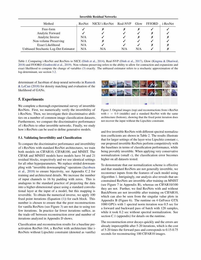
Figure 3. Original images (top) and reconstructions from i-ResNetwith c = 0.9 (middle) and a standard ResNet with the samearchitecture (bottom), showing that the fixed point iteration doesnot recover the input without the Lipschitz constraint.

and five invertible ResNets with different spectral normaliza-tion coefficients are shown in Table 2. The results illustratethat for larger settings of the layer-wise Lipschitz constant c,our proposed invertible ResNets perform competitively withthe baselines in terms of classification performance, whilebeing provably invertible. When applying very conservativenormalization (small c), the classification error becomeshigher on all datasets tested.

To demonstrate that our normalization scheme is effectiveand that standard ResNets are not generally invertible, wereconstruct inputs from the features of each model usingAlgorithm 1. Intriguingly, our analysis also reveals that un-constrained ResNets are invertible after training on MNIST(see Figure 7 in Appendix B), whereas on CIFAR10/100they are not. Further, we find ResNets with and withoutBatchNorm are not invertible after training on CIFAR10,which can also be seen from the singular value plots inAppendix B (Figure 6). The runtime on 4 GeForce GTX1080 GPUs with 1 spectral norm iteration was 0.5 sec fora forward and backward pass of batch with 128 samples,while it took 0.2 sec without spectral normalization. Seesection C.1 (appendix) for details on the runtime.

The reconstruction error decays quickly and the errors arealready imperceptible after 5-20 iterations, which is the costof 5-20 times the forward pass and corresponds to 0.15-0.75seconds for reconstructing 100 CIFAR10 images.

Invertible Residual Networks

ResNet-164 Vanilla c = 0.9 c = 0.8 c = 0.7 c = 0.6 c = 0.5

Classification MNIST - 0.38 0.40 0.42 0.40 0.42 0.86Error % CIFAR10 5.50 6.69 6.78 6.86 6.93 7.72 8.71

CIFAR100 24.30 23.97 24.58 24.99 25.99 27.30 29.45

Guaranteed Inverse No No Yes Yes Yes Yes Yes

Table 2. Comparison of i-ResNet to a ResNet-164 baseline architecture of similar depth and width with varying Lipschitz constraints viacoefficients c. Vanilla shares the same architecture as i-ResNet, without the Lipschitz constraint.

Computing the inverse is fast even for the largest normaliza-tion coefficient, but becomes faster with stronger normaliza-tion. The number of iterations needed for full convergenceis approximately cut in half when reducing the spectralnormalization coefficient by 0.2, see Figure 8 (AppendixD) for a detailed plot. We also ran an i-RevNet (Jacobsenet al., 2018) with comparable hyperparameters as ResNet-164 and it performs on par with ResNet-164 with 5.6%.Note however, that i-RevNets, like NICE (Dinh et al., 2014),are volume-conserving, making them less well-suited togenerative modeling.

In summary, we observe that invertibility without additionalconstraints is unlikely, but possible, whereas it is hard topredict if networks will have this property. In our proposedmodel, we can guarantee the existence of an inverse withoutsignificantly harming classification performance.

5.2. Comparison with Other Invertible Architectures

In this section we compare i-ResNet classifiers to the state-of-the-art invertible flow-based model Glow. We take theimplementation of Kingma & Dhariwal (2018) and modifyit to classify CIFAR10 images (with no generative mod-eling component). We create an i-ResNet that is as closeas possible in structure to the default Glow model on CI-FAR10 (denoted as i-ResNet Glow-style) and compare itto two variants of Glow, one that uses learned (1 × 1 con-volutions) and affine block structure, and one with reversepermutations (like Real-NVP) and additive block structure.Results of this experiment can be found in Table 3. We cansee that i-ResNets outperform all versions of Glow on this

Affine Glow Additive Glow i-ResNet i-ResNet1 × 1 Conv Reverse Glow-Style 164

12.63 12.36 8.03 6.69

Table 3. CIFAR10 classification results compared to state-of-the-art flow Glow as a classifier. We compare two versions of Glow, aswell as an i-ResNet architecture as similar as possible to Glow inits number of layers and channels, termed “i-ResNet, Glow-Style”.

discriminative task, even when adapting the network depthand width to that of Glow. This indicates that i-ResNetshave a more suitable inductive bias in their block structurefor discriminative tasks than Glow.

We also find that i-ResNets are considerably easier to trainthan these other models. We are able to train i-ResNetsusing SGD with momentum and a learning rate of 0.1whereas all version of Glow we tested needed Adam orAdamax (Kingma & Ba, 2014) and much smaller learningrates to avoid divergence.

5.3. Generative Modeling

We run a number of experiments to verify the utility of i-ResNets in building generative models. First, we comparei-ResNet Flows with Glow (Kingma & Dhariwal, 2018)on simple two-dimensional datasets. Figure 2 qualitativelyshows the density learned by a Glow model with 100 cou-pling layers and 100 invertible linear transformations. Wecompare against an i-ResNet where the coupling layers arereplaced by invertible residual blocks with the same numberof parameters and the invertible linear transformations arereplaced by actnorm (Kingma & Dhariwal, 2018). Thisresults in the i-ResNet model having slightly fewer parame-ters, while maintaining an equal number of layers. In thisexperiment we train i-ResNets using the brute-force com-puted log-determinant since the data is two-dimensional.We find that i-ResNets are able to more accurately fit thesesimple densities. As stated in Grathwohl et al. (2019), webelieve this is due to our model’s ability to avoid partitioningdimensions.

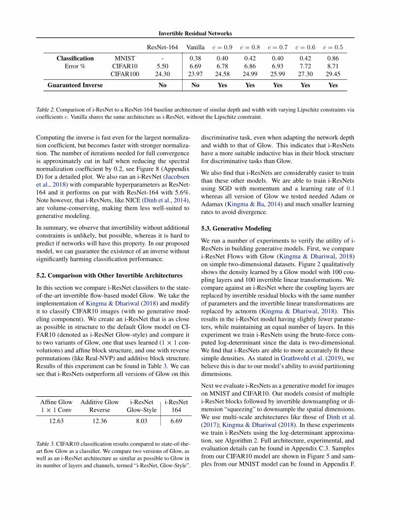
Next we evaluate i-ResNets as a generative model for imageson MNIST and CIFAR10. Our models consist of multiplei-ResNet blocks followed by invertible downsampling or di-mension “squeezing” to downsample the spatial dimensions.We use multi-scale architectures like those of Dinh et al.(2017); Kingma & Dhariwal (2018). In these experimentswe train i-ResNets using the log-determinant approxima-tion, see Algorithm 2. Full architecture, experimental, andevaluation details can be found in Appendix C.3. Samplesfrom our CIFAR10 model are shown in Figure 5 and sam-ples from our MNIST model can be found in Appendix F.

Invertible Residual Networks

Method MNIST CIFAR10

NICE (Dinh et al., 2014) 4.36 4.48†MADE (Germain et al., 2015) 2.04 5.67MAF (Papamakarios et al., 2017) 1.89 4.31Real NVP (Dinh et al., 2017) 1.06 3.49Glow (Kingma & Dhariwal, 2018) 1.05 3.35FFJORD (Grathwohl et al., 2019) 0.99 3.40

i-ResNet 1.06 3.45

Table 4. MNIST and CIFAR10 bits/dim results. † Uses ZCA pre-processing making results not directly comparable.

Compared to the classification model, the log-determinantapproximation with 5 series terms roughly increased thecomputation times by a factor of 4. The bias and varianceof our log-determinant estimator is shown in Figure 4.

Results and comparisons to other generative models can befound in Table 4. While our models did not perform as wellas Glow and FFJORD, we find it intriguing that ResNets,with very little modification, can create a generative modelcompetitive with these highly engineered models. We be-lieve the gap in performance is mainly due to our use ofa biased log-determinant estimator and that the use of anunbiased method (Han et al., 2018) can help close this gap.

6. Other ApplicationsIn many applications, a secondary unsupervised learning orgenerative modeling objective is formulated in combinationwith a primary discriminative task. i-ResNets are appealinghere, as they manage to achieve competitive performanceon both discriminative and generative tasks. We summarizesome application areas to highlight that there is a widevariety of tasks for which i-ResNets would be promising toconsider:

• Hybrid density and discriminative models for joint clas-sification and detection or fairness applications (Nalis-

Figure 4. Bias and standard deviation of our log-determinant esti-mator as the number of power series terms increases. Variance isdue to the stochastic trace estimator.

Figure 5. CIFAR10 samples from our i-ResNet flow. More samplescan be found in Appendix F.

nick et al., 2018; Louizos et al., 2016)

• Unsupervised learning for downstream tasks (Hjelmet al., 2019; Van Den Oord et al., 2018)

• Semi-supervised learning from few labeled examples(Oliver et al., 2018; Kingma et al., 2014)

• Solving inverse problems with hybrid regression andgenerative losses (Ardizzone et al., 2019)

• Adversarial robustness with likelihood-based genera-tive models (Schott et al., 2019; Jacobsen et al., 2019)

Finally, it is plausible that the Lipschitz bounds on the layersof the i-ResNet could aid with the stability of gradients foroptimization, as well as adversarial robustness.

7. ConclusionsWe introduced a new architecture, i-ResNets, which allowfree-form layer architectures while still providing tractabledensity estimates. The unrestricted form of the Jacobianallows expansion and contraction via the residual blocks,while partitioning-based models (Dinh et al., 2014; 2017;Kingma & Dhariwal, 2018) must include affine blocks andscaling layers to be non-volume preserving.

Several challenges remain to be addressed in future work.First, our estimator of the log-determinant is biased. How-ever, there have been recent advances in building unbiasedestimators for the log-determinant (Han et al., 2018), whichwe believe could improve the performance of our generativemodel. Second, learning and designing networks with aLipschitz constraint is challenging. For example, we needto constrain each linear layer in the block instead of beingable to directly control the Lipschitz constant of a block, seeAnil et al. (2018) for a promising approach for addressingthis problem.

AcknowledgmentsWe thank Rich Zemel for very helpful comments on anearlier version of the manuscript. We thank Yulia Rubanova

Invertible Residual Networks

for spotting a mistake in one of the proofs. We also thankeveryone else at Vector for helpful discussions and feedback.

We gratefully acknowledge the financial support from theGerman Science Foundation for RTG 2224 ”π3: ParameterIdentification - Analysis, Algorithms, Applications”

ReferencesAdams, R. P., Pennington, J., Johnson, M. J., Smith, J.,

Ovadia, Y., Patton, B., and Saunderson, J. Estimating thespectral density of large implicit matrices. arXiv preprintarXiv:1802.03451, 2018.

Anil, C., Lucas, J., and Grosse, R. Sorting out lipschitz func-tion approximation. arXiv preprint arXiv:1811.05381,2018.

Ardizzone, L., Kruse, J., Rother, C., and Kothe, U. Analyz-ing inverse problems with invertible neural networks. InInternational Conference on Learning Representations,2019.

Ascher, U. Numerical methods for evolutionary differen-tial equations. Computational science and engineering.Society for Industrial and Applied Mathematics, 2008.

Avron, H. and Toledo, S. Randomized algorithms for esti-mating the trace of an implicit symmetric positive semi-definite matrix. J. ACM, 58(2):8:1–8:34, 2011.

Boutsidis, C., Drineas, P., Kambadur, P., Kontopoulou, E.-M., and Zouzias, A. A randomized algorithm for ap-proximating the log determinant of a symmetric positivedefinite matrix. Linear Algebra and its Applications, 533:95 – 117, 2017.

Chang, B., Meng, L., Haber, E., Ruthotto, L., Begert, D.,and Holtham, E. Reversible architectures for arbitrar-ily deep residual neural networks. Thirty-Second AAAIConference on Artificial Intelligence, 2018.

Chen, T. Q., Rubanova, Y., Bettencourt, J., and Duvenaud,D. Neural ordinary differential equations. Advances inNeural Information Processing Systems, 2018.

Ciccone, M., Gallieri, M., Masci, J., Osendorfer, C., andGomez, F. Nais-net: Stable deep networks from non-autonomous differential equations. In Advances in Neu-ral Information Processing Systems 31, pp. 3029–3039.2018.

Clevert, D., Unterthiner, T., and Hochreiter, S. Fast and ac-curate deep network learning by exponential linear units(elus). arXiv preprint arXiv:1511.07289, 2015.

Dinh, L., Krueger, D., and Bengio, Y. Nice: Non-linearindependent components estimation. arXiv preprintarXiv:1410.8516, 2014.

Dinh, L., Sohl-Dickstein, J., and Bengio, S. Density es-timation using real nvp. International Conference onLearning Representations, 2017.

Dong, K., Eriksson, D., Nickisch, H., Bindel, D., and Wil-son, A. G. Scalable log determinants for gaussian processkernel learning. In Advances in Neural Information Pro-cessing Systems 30, pp. 6327–6337. 2017.

Germain, M., Gregor, K., Murray, I., and Larochelle, H.MADE: Masked autoencoder for distribution estimation.In ICML, volume 37 of JMLR Workshop and ConferenceProceedings, pp. 881–889. JMLR.org, 2015.

Gomez, A. N., Ren, M., Urtasun, R., and Grosse, R. B.The reversible residual network: Backpropagation with-out storing activations. Advances in Neural InformationProcessing Systems, 2017.

Gouk, H., Frank, E., Pfahringer, B., and Cree, M. Regulari-sation of neural networks by enforcing lipschitz continu-ity. arXiv preprint arXiv:1804.04368, 2018.

Grathwohl, W., Chen, R. T. Q., Bettencourt, J., and Duve-naud, D. Ffjord: Scalable reversible generative modelswith free-form continuous dynamics. In InternationalConference on Learning Representations, 2019.

Haber, E. and Ruthotto, L. Stable architectures for deepneural networks. Inverse Problems, 34(1):014004, 2018.

Hall, B. C. Lie groups, lie algebras, and representations: Anelementary introduction. Graduate Texts in Mathematics,222 (2nd ed.), Springer, 2015.

Han, I., Malioutov, D., Avron, H., and Shin, J. Approxi-mating the spectral sums of large-scale matrices usingchebyshev approximations. SIAM Journal on ScientificComputing, 39, 06 2016.

Han, I., Avron, H., and Shin, J. Stochastic chebyshev gradi-ent descent for spectral optimization. In Advances in Neu-ral Information Processing Systems 31, pp. 7397–7407.2018.

He, K., Zhang, X., Ren, S., and Sun, J. Deep residual learn-ing for image recognition. In Proceedings of the IEEEconference on computer vision and pattern recognition,pp. 770–778, 2016.

Hjelm, R. D., Fedorov, A., Lavoie-Marchildon, S., Grewal,K., Bachman, P., Trischler, A., and Bengio, Y. Learningdeep representations by mutual information estimationand maximization. In International Conference on Learn-ing Representations, 2019.

Hutchinson, M. A stochastic estimator of the trace of theinfluence matrix for laplacian smoothing splines. Com-munications in Statistics - Simulation and Computation,19(2):433–450, 1990.

Invertible Residual Networks

Jacobsen, J.-H., Smeulders, A. W., and Oyallon, E. i-revnet:Deep invertible networks. In International Conferenceon Learning Representations, 2018.

Jacobsen, J.-H., Behrmann, J., Zemel, R., and Bethge, M.Excessive invariance causes adversarial vulnerability. InInternational Conference on Learning Representations,2019.

Karras, T., Laine, S., and Aila, T. A style-based generatorarchitecture for generative adversarial networks. arXivpreprint arXiv:1812.04948, 2018.

Kingma, D. P. and Ba, J. Adam: A method for stochasticoptimization. arXiv preprint arXiv:1412.6980, 2014.

Kingma, D. P. and Dhariwal, P. Glow: Generative flowwith invertible 1x1 convolutions. Advances in NeuralInformation Processing Systems, 2018.

Kingma, D. P., Mohamed, S., Rezende, D. J., and Welling,M. Semi-supervised learning with deep generative mod-els. In Advances in neural information processing sys-tems, pp. 3581–3589, 2014.

Louizos, C., Swersky, K., Li, Y., Welling, M., and Zemel,R. The variational fair autoencoder. International Con-ference on Learning Representations, 2016.

Lu, Y., Zhong, A., Li, Q., and Dong, B. Beyond fi-nite layer neural networks: Bridging deep architecturesand numerical differential equations. arXiv preprintarXiv:1710.10121, 2017.

Miyato, T., Kataoka, T., Koyama, M., and Yoshida, Y. Spec-tral normalization for generative adversarial networks. InInternational Conference on Learning Representations,2018.

Nalisnick, E., Matsukawa, A., Teh, Y. W., Gorur, D., andLakshminarayanan, B. Hybrid models with deep andinvertible features. NeurIPS workshop on Bayesian deeplearning, 2018.

Oliver, A., Odena, A., Raffel, C. A., Cubuk, E. D., and Good-fellow, I. Realistic evaluation of deep semi-supervisedlearning algorithms. In Advances in Neural InformationProcessing Systems 31. 2018.

Papamakarios, G., Murray, I., and Pavlakou, T. Maskedautoregressive flow for density estimation. In Advancesin Neural Information Processing Systems, 2017.

Parmar, N., Vaswani, A., Uszkoreit, J., Kaiser, L., Shazeer,N., Ku, A., and Tran, D. Image transformer. In ICML, vol-ume 80 of JMLR Workshop and Conference Proceedings,pp. 4052–4061. JMLR.org, 2018.

Ramesh, A. and LeCun, Y. Backpropagation for implicitspectral densities. arXiv preprint arXiv:1806.00499,2018.

Rezende, D. J. and Mohamed, S. Variational inferencewith normalizing flows. Proceedings of the 32nd In-ternational Conference on International Conference onMachine Learning, 2015.

Ruthotto, L. and Haber, E. Deep neural networks moti-vated by partial differential equations. arXiv preprintarXiv:1804.04272, 2018.

Schott, L., Rauber, J., Bethge, M., and Brendel, W. To-wards the first adversarially robust neural network modelon MNIST. In International Conference on LearningRepresentations, 2019.

Sedghi, H., Gupta, V., and Long, P. M. The singular valuesof convolutional layers. In International Conference onLearning Representations, 2019.

Sokoli, J., Giryes, R., Sapiro, G., and Rodrigues, M. R. D.Robust large margin deep neural networks. IEEE Trans-actions on Signal Processing, 65(16):4265–4280, 2017.

Tsuzuku, Y., Sato, I., and Sugiyama, M. Lipschitz-margintraining: Scalable certification of perturbation invariancefor deep neural networks. Advances in Neural Informa-tion Processing Systems, 2018.

Van Den Oord, A., Dieleman, S., Zen, H., Simonyan, K.,Vinyals, O., Graves, A., Kalchbrenner, N., Senior, A., andKavukcuoglu, K. Wavenet: A generative model for rawaudio. arXiv preprint arXiv:1609.03499, 2016a.

Van Den Oord, A., Kalchbrenner, N., and Kavukcuoglu, K.Pixel recurrent neural networks. In Proceedings of the33rd International Conference on International Confer-ence on Machine Learning - Volume 48, pp. 1747–1756,2016b.

Van Den Oord, A., Li, Y., and Vinyals, O. Representa-tion learning with contrastive predictive coding. arXivpreprint arXiv:1807.03748, 2018.

Withers, C. S. and Nadarajah, S. log det a = tr log a. Inter-national Journal of Mathematical Education in Scienceand Technology, 41(8):1121–1124, 2010.

Zagoruyko, S. and Komodakis, N. Wide residual networks.arXiv preprint arXiv:1605.07146, 2016.