Download - Investigating Climate Change Impact on stream …...INVESTIGATING CLIMATE CHANGE IMPACT ON STREAM FLOW OF BARO-AKOBO RIVER BASIN CASE STUDY OF BARO CATCHMENT. 1 Shimelash Molla, 2

GSJ: VOLUME 6, ISSUE 5, MAY 2018 1

GSJ© 2018 www.globalscientificjournal.com

GSJ: Volume 6, Issue 5, May 2018, Online: ISSN 2320-9186

www.globalscientificjournal.com

INVESTIGATING CLIMATE CHANGE IMPACT ON

STREAM FLOW OF BARO-AKOBO RIVER BASIN

CASE STUDY OF BARO CATCHMENT. 1Shimelash Molla, 2Tolera Abdisa, 3Tamene Adugna (Dr.Ing)

Civil Engineering Department, Mettu University, Mettu, Ethiopia

ABSTRACT

In recent decades changes in climate have caused impacts on natural and human systems on all continents and

across the oceans. Impacts are due to observed climate change, irrespective of its cause, indicating the sensitivity of

natural and human systems to changing climate. One of the direct impacts of this climate change is on water

resources development and indirectly for agricultural production, environmental quality and economic development

which will lead again to difficult conditions for Human to live in. The objective of this thesis is to assess the impact of

climate change on the stream flow of Baro watershed which is the major tributary of Baro-Akobo basin, Ethiopia. The

soil and water assessment tool (SWAT) model was used to simulate the stream flow using the meteorological data of

thirty one years from 1986 to 2016. The model was calibrated for a period of sixteen years from 1990-2005 and

validated for the observed data for eleven years from 2006-2015 and shows a good agreement with R2 = 0.90 during

calibration and R2= 0.93 during validation whereas NSE=0.66 during calibration and 0.61 during validation.

Hypothetical climate change scenarios of precipitation from -20% to +20% at 10% interval and temperature change

from 2oC ,and 3oC for the period of 2050s and from 3.5oC to 6oC at 1.5oC interval for the period of 2080s under

RCPs 8.5 was taken based on the IPCC 5th assessment set for African countries. Results of this procedure show the

sensitivity of stream flow to climate variability. For example, a change of precipitation from -20% to +20% for

constant temperature of 2oC gives a reduction of stream flow by around 11% .Beside this, for a constant

precipitation of 0% and variation of temperature from 2oC to 3oC there is reduction of stream flow by average of

12.7%. This shows that the Baro Catchment will be more sensitive to the average increase in temperature than to the

average decrease in rainfall, which shows the role of evapotranspiration in the water cycle. Overall, the result

suggest, a decrease in stream flow of 12.73% for the period of 2050s (i.e.2046-2065) and 15.56% by the end of the

21st century (2080s) as a consequence of decreasing rainfall of -20% and increasing temperature of 6oC Scenarios

(i.e. the worst scenarios) .

Key words: Baro Watershed, Synthetic scenario, RCP, Climate, SWAT, SWAT-CUP

http://www.globalscientificjournal.com/



1. INTRODUCTION

Background

Evidence of observed climate change

impacts is strongest and most

comprehensive for natural systems.

Changing of precipitation or melting snow

and ice are changing hydrological systems

in many regions, affecting water resources

in terms of quantity and quality. Many

terrestrial, fresh water, and marine species

have shifted their geomorphic ranges ,

seasonal activities, migration patterns,

abundances, and species interactions in

response to ongoing climate change

(IPCC, 2014) .Some impacts on human

systems have also been attributed to

climate change, with a major or minor

contribution of climate change

distinguished from other influences. The

negative impacts change on crop yields

has been more common than positive

impacts according to the assessments of

many studies covering a wide range of

regions and crops.

Climate changes have had observable

impacts on the natural systems. Climate

change is expected to worsen current

stresses on water resources availability

from population growth, urbanization and

land-use change (Liben, 2011). A major

effect of climate change is likely to be

interchanges in hydrologic cycles and

changes in water availability. Increased

evaporation, combined with changes in

precipitation, has the potential to affect

runoff, the frequency and intensity of

floods and droughts, soil moisture and

available water for irrigation and

hydroelectric power generation.

The global increase in water resources

demand due to lifestyle change and

population growth is affected by

freshwater scarcity throughout the planet.

Meanwhile, the potential effects of climate

change on water resources availability

increase further challenges on the

sustainability of this insufficient yet life-

dependent substance; this is in addition to

the complexity of the prospect of climate’s

natural variability and its eventual reserved

effect on the water balance cycle

(Ramadan, 2012). As this is a decades old

subject of on-going discussion in the

global scientific community, the

Intergovernmental Panel for Climate

Change (IPCC) recently emphasized the

need for directing climate variability and

change impacts on water resources studies

toward regional and local dimensions. To

be consistent with local population

demands and priorities this allows for the

creation of competent mitigation solutions.

Continued emission of greenhouse gases

will cause further warming and on-going

changes in all components of the climate



system, increasing the likelihood of severe,

pervasive and irreversible impacts for

people and ecosystems. Limiting climate

change would require considerable and

continual reductions in greenhouse gas

emissions which, together with adaptation,

can limit climate change risks.

According to IPCC 2014 Surface

temperature is projected to rise over the

21st century under all assessed emission

scenarios. It is very likely that heat waves

will occur more often and last longer, and

that extreme precipitation events will

become more intense and frequent in many

regions. The ocean will continue to warm

and acidify, and global mean sea level to

rise. Accordingly to this report (IPCC,

2014),the global mean surface temperature

change for the period 2016-2035 will

likely be in the range 0.3°C-0.7°C

(medium confidence). Relative to 1850-

1900, global surface temperature change

for the end of the 21st century (2081-2100)

is projected to likely exceed 1.5°C (high

confidence). It is virtually certain that

there will be more frequent hot and fewer

cold temperature extremes over most land

areas on daily and seasonal timescales, as

global mean surface temperature increases

(Allen et al., 2014).

Developing countries in general and least

developed countries like Ethiopia in

particular are more exposed to the adverse

impacts of climate variability and change.

This is due to their low adaptive capacity

and high sensitivity of their socio-

economic systems to climate variability

and change (Elshamy, 2010).

From the point of view of the design and

management of water resource systems,

hydrologists are required to make accurate

predictions of the impacts of climate

change on the intensity, amount, and

spatial and temporal variability of rainfall.

Furthermore, and possibly most important,

they also must examine how the stream

flow regime (e.g., stream flow

hydrographs, peak flow ,etc.) at different

spatial and temporal scales is affected by

rainfall variability and by the expected

changes in that variability as a result of

climate change (Ramirez et al., 2007).

One of the most important impacts on

society of future climatic changes will be

changes in regional water availability

(Chong-yu Xu, 1999). Such hydrologic

changes will affect nearly every aspect of

human well-being, from agricultural

productivity and energy use to flood

control, municipal and industrial water

supply, and fish and wildlife management.

The great importance of water in both

society and nature underscores the

necessity of understanding how a change

in global climate could affect regional

water supplies.



According to the Intergovernmental Panel

on Climate Change (IPCC) 5th assessment

report (Isabelle, 2014) global average

surface temperature would likely rise

between 3°C to 6°C by 2100 with the

RCPs of 8.5 and rise by 2oc to 3

oc with the

RCPs of 4.5. With respect to precipitation,

the results are different for different

regions; the report also indicates that an

increase in mean annual rainfall in East

Africa is likely. The minimum temperature

over Ethiopia show an increase of about

0.37°C per decade, which indicates the

signal of warming over the period of the

analysis 1957-2005 (Di Baldassarre,

2011). Previous studies in Nile basin

provide different indication regarding long

term rainfall trends; (Elshamy ME, 2009)

reported future precipitation change in the

Blue Nile is uncertain in their assessment

of climate change on stream flow of the

Blue Nile for 2081-2098 period using 17

GCMs. (Wing H, 2008) showed that there

are no significant changes or trends in

annual rainfall at the national or watershed

level in Ethiopia.

The successful realisation of any water

resources activity is important to a country

like Ethiopia for the growth of the national

economy. Among the twelve river basins

in Ethiopia, the Baro-Akobo basin has

abundant water resources which up to now

have not been developed to any significant

level. The Baro-Akobo basin has of great

unrealized potential, under populated by

Ethiopian standard, and with plenty of land

and water. The abundance of water

combined with the relief of the basin, from

the high plateau at above 2,500m elevation

down to the Gambella plain at an altitude

of 430m provides favourable conditions

for hydropower in this region. The river

Baro-Akobo is used for water supply for

domestic and industrial uses, irrigation,

hydropower generation and navigation.

Of the tributaries of the Basin, Baro-river

is the major one. The Baro River is created

by the confluence of the Birbir and Gebba

Rivers, east of Metu in the Illubabor Zone

of the Oromia Region. From its source in

the Ethiopian Highlands it flows west for

306 kilometres (190 mi) to join the Pibor

River. The Baro-Pibor confluence marks

the beginning of the Sobat River, a

tributary of the White Nile.

.



Statement of the problem

By 2025, it is estimated that around 5

billion people, out of a total population of

around 8 billion, will be living in countries

suffering water shortage (using more than

20% of their available resources) (Arnell,

1999).

Climate warming observed over the past

several decades is consistently associated

with changes in a number of components

of the hydrological cycle and hydrological

systems such as: changing precipitation

patterns, intensity and extremes;

widespread melting of snow and ice;

increasing atmospheric water vapour;

increasing evaporation; and changes in soil

moisture and runoff (Abera, 2011).

There is abundant evidence from

observational records and climate

projections that freshwater resources are

susceptible and have the potential to be

strongly impacted by climate change.

However, the ability to quantify future

changes in hydrological variables, and

their impacts on systems and sectors, is

limited by uncertainty at all stages of the

assessment process. Uncertainty comes

from the range of socio-economic

development scenarios, the downscaling of

climate effects to local/regional scales,

impact assessments, and feedbacks from

adaptation and mitigation activities.

Decision making needs to operate in the

context of this uncertainty. Robust

methods to assess risks based on these

uncertainties are at an early stage of

development (Bates, 2008)).

This impact of climate change affects

more developing countries in general and

least developing countries like Ethiopia in

particular, due to their low adaptive

capacity and high sensitivity of their socio-

economic systems to climate variability

and change. Current climate variability is

already imposing a significant challenge to

Ethiopia by affecting food security, water

and energy supply, poverty reduction and

sustainable development efforts, as well

as by causing natural resource degradation

and natural disasters (Abebe, 2007).

Among the river basins of Ethiopia which

are affected by climate change Baro-

Akobo river basin is one of them (Kebede,

2013), in which Baro river is the major

tributary. Therefore in this study the

impact of climate changes on the Baro-

River was assessed. This is used to have a

good in sight for checking the possible

impact of climate change in the basin in

the future.



Objectives

1.1.1. General Objective

The general obvective of this study is to

assess the impact of climate change on

streamflow of the Baro river by taking

different scenarios.

1.1.2. Specific Objective

The following specific objectives are set in

order to come to the main objective.

To develop hydrologic SWAT

model for the Baro-Watershed.

To assess the impact of

precipitation and temprature for the

future period as compared to the

baseline period based on the

synthetic scenarios.

To quantify the possible impacts of

climate change on the hydrology of

the catchment based on synthetic

scenarios set by IPCC 5th

assessment report.

2. Method and Materials

2.1. Description of the Study Area

Baro-Akobo Basin lies in the southwest of

Ethiopia between latitudes of 5° 31` and

10° 54` N, and longitudes of 33° 0` and

36° 17` E. The basin area is about 76,000

km2 and is bordered by the Sudan in the

West, northwest and southwest, Abbay and

Omo-Gibe Basins in the east. The major

rivers within the Baro-Akobo basin are

Baro and its tributaries Alwero, Gilo and

the Akobo. These rivers, which arise in the

eastern part of the highlands, flow

westward to join the White Nile in Sudan.

The mean annual runoff of the basin is

estimated to be about 23 km3 as gauged at

Gambella station. Elevation of the study

area varies between 440 and 3000 m

a.m.s.l. The higher elevation ranges are

located in the North East and Eastern part

of the basin while the remaining part of the

basin is found in lower elevation. In the

study area, there is high variability in

temperature with large differences

between the daily maximum and minimum

temperatures.

One of the tributaries of the Baro River is

a river in southwestern Ethiopia, which

defines part of Ethiopia's border with

South Sudan. The Baro River is created by

the confluence of the Birbir and Gebba



Rivers, east of Metu in the Illubabor Zone

of the Oromia Region. From its source in

the Ethiopian Highlands it flows west for

306 kilometers (190 mi) to join the Pibor

River. The Baro-Pibor confluence marks

the beginning of the Sobat River, a

tributary of the White Nile. The Baro and

its tributaries drain a watershed 41,400

km2 (16,000 sq. mi) in size. The river's

mean annual discharge at its mouth is 241

m³/s (8,510 ft³/s).In this thesis the impact

of climate change on this river is going to

be assessed which will be a representative

of the basin since it covers most of the area

of the basin.

Figure. 2.1. Location of Baro Watershed

\

2.2. Hydrologic Modeling

A physically based hydrological model

was used for the Baro catchment to assess

the impact of climate change on the area.

Soil and Water Assessment tool (SWAT)

was selected as the best modeling tool

owing to many reasons. First and for most

it is a public domain model and it is used

for free. Secondly in countries like

Ethiopia, there is a shortage of long term

observational data series to use

sophisticated models; however, SWAT is

computationally efficient and requires

minimum data. Besides SWAT was

checked in the highlands of Ethiopia and

gave satisfactory results (Setegn Shimelsi,

2008). SWAT model was developed to

predict the impact of land management

practices on water, sediment, and

agricultural chemical yields. However, this

study concentrated on the hydrological

aspect of the basin. The description of the

model, model inputs and model setup are

discussed in detail in the subsequent

sections.



2.2.1 Soil and Water Assessment Tool

(SWAT) Background

SWAT is a river basin scale model

developed to quantify the impact of land

management practices on water, sediment

and agricultural chemical yields in large

complex watersheds with varying soils,

land use and management conditions over

long periods of time. The main

components of SWAT include weather,

surface runoff, return flow, percolation,

evapotranspiration, transmission losses,

pond & reservoir storage, crop growth &

irrigation, groundwater flow, reach

routing, nutrient & pesticide loading, and

water transfer. It is a public domain model

actively supported by the USDA

Agricultural Research Service at the

Grassland, Soil and Water Research

Laboratory in Temple, Texas.

SWAT requires specific information about

weather, soil properties, topography,

vegetation, and land management practices

occurring in the watershed. The minimum

data required to make a run are commonly

available from government agencies. From

this a number of output files are generated

by SWAT. These files can be grouped by

the type of data stored in the file as

standard output file (.std), the Hydrologic

Response Units (HRU) output file (.sbs),

the sub-basin output file (.bsb), and the

main channel or reach output file (.rch).

In order to setup the model, the digital

elevation model, land use/land cover and

soil map were projected into common

projection system. Model has capability to

delineate the DEM into watershed or basin

and divided into sub-basin. The layers of

land use/land cover, soil, map and slopes

categories were overlaid and reclassified

into hydrological response unit (HRUs).

Hydrologic response units (HRUs) have

been defined as the unique combination of

specific land use, soil and slope

characteristics (Arnold, 1998).The model

estimates the hydrologic components such

as evapotranspiration, surface runoff, peak

rate of runoff and other components on the

basis of each HRUs unit. Water is then

routed from HRUs to sub-basin and sub-

basin to watershed (Tripathi.M.P, 2003).

The equation of mass balance performed at

the HRU level is given as follows:

------------------------------------------2.1

Where St is the final storage (mm), So is

the initial storage in day i (mm), t is the

time (days), Rday is the rainfall (mm/day),

Qsurf is the surface runoff (mm/day), Ea is

evapotranspiration (mm/day), Wseep is

seepage rate (mm/day) and Qgw is return

flow (mm/day).

In order to estimate the surface runoff,

there were two methods available: SCS

curve number (Soil Conservation Service)



and Green and Ampt infiltration method.

In this study, the SCS curve number

method was used to estimate surface

runoff. The SCS curve number is

described by the following equation:

----------------------2.2.

Where Qsurf is accumulated runoff or

rainfall excess (mm/day), Rday is the

rainfall depth (mm/day) and S is the

retention parameter (mm). The retention

parameter is defined by the following

equation:

-----------------------2.3.

SWAT provides three methods that can be

used to calculate potential evaporation

(PET). These are the Penman-Monteith

method, the priestly-Taylor method and

the Hargreaves method. The model can

also read in daily PET values if the user

prefers to apply a different potential

evapotranspiration method. The three PET

methods vary in the amount of required

inputs. The Penman-Monteith method

requires solar radiation, air temperature,

relative humidity and wind speed. The

Priestley-Taylor method requires solar

radiation, air temperature and relative

humidity. The Hargreaves method requires

air temperature only. In this study, among

the three methods, Penman-Monteith

Method was used to estimate PET values

(Neitsch S.L., 2005).

2.3. SWAT Model Inputs Data

The SWAT Model requires input data’s

such as DEM of the study area,

topography, soil, land use and

meteorological data including daily

rainfall, minimum and maximum

temperature, relative humidity, solar

radiation and wind speed for the analysis

of the watershed.

2.3.1. Digital Elevation Model

The Digital Elevation Model (DEM) is any

digital representation of a topographic

surface and specifically to a raster or

regular grid of spot heights. It is the basic

input of SWAT hydrologic model to

delineate watersheds and River networks.

The first step in creating the model input is

the watershed delineation accomplished

using digital elevation data. DEM is the

first input of SWAT model for delineating

the watershed to be modeled. Based on

threshold specifications and the DEM, the

SWAT Arc View interface was used to

delineate the watershed into sub basins and

subsequently, sub basins were divided into

Hydrologic Response Units (HRU)

The DEM was also used to analyze the

drainage patterns of the land surface

terrain. Sub basin parameters such as slope

gradient, slope length of the terrain, and



the stream network characteristics such as

channel slope, length, and width were

derived from the DEM.

The catchment physiographic data were

generally collected from topographic maps

and 90mx90m resolution DEM. This DEM

data was obtained from GIS data that

found in Ministry of Water and Energy

directorate of GIS. This DEM data was

basic input for the water shed delineation

and slope calculation of the basin in the

SWAT model processing.

Figure 2.2. Digital elevation model for

Baro River extracted from Ethio- DEM.

3.3.2. Land Use Land Cover Data

SWAT requires the land use land cover

data to define the Hydrological Responses

Units (HRU). The land use land cover map

of the study area was obtained from the

ministry of water resources GIS

department. Based on these data the

SWAT major land use land cover map was

produced by overlying the land use shape

files. Then after the major land use land

cover classification were sub divided into

sub classes mainly based on dominant

crops for cultivated lands. Then SWAT

calculated the area covered by each land

use. The different land use/land cover

types are presented in table 3.1.

Figure.2.3. Land use/cover of Baro

Watershed



Table 2.1. SWAT Major Land Use

Classes, Codes and Areal Coverage of

Baro Watershed

Land use SWA

T

code

Area(km

2)

%watersh

ed area

Agricultur

al Land -

Generic

AGR

L

5073.82 21.24

Agricultur

al Land-

Row

Crops

AGR

R

208.64 0.87

Agricultur

al Land-

Close-

grown

AGR

C

9489.46 39.73

Forest -

Deciduou

s

FRS

D

940.81 3.94

Alamo –

Switch

grass

SWC

H

263.05 1.10

Eucalyptu

s

EUC

A

169.75 0.71

Forest-

Mixed

FRST 7738.3 32.40

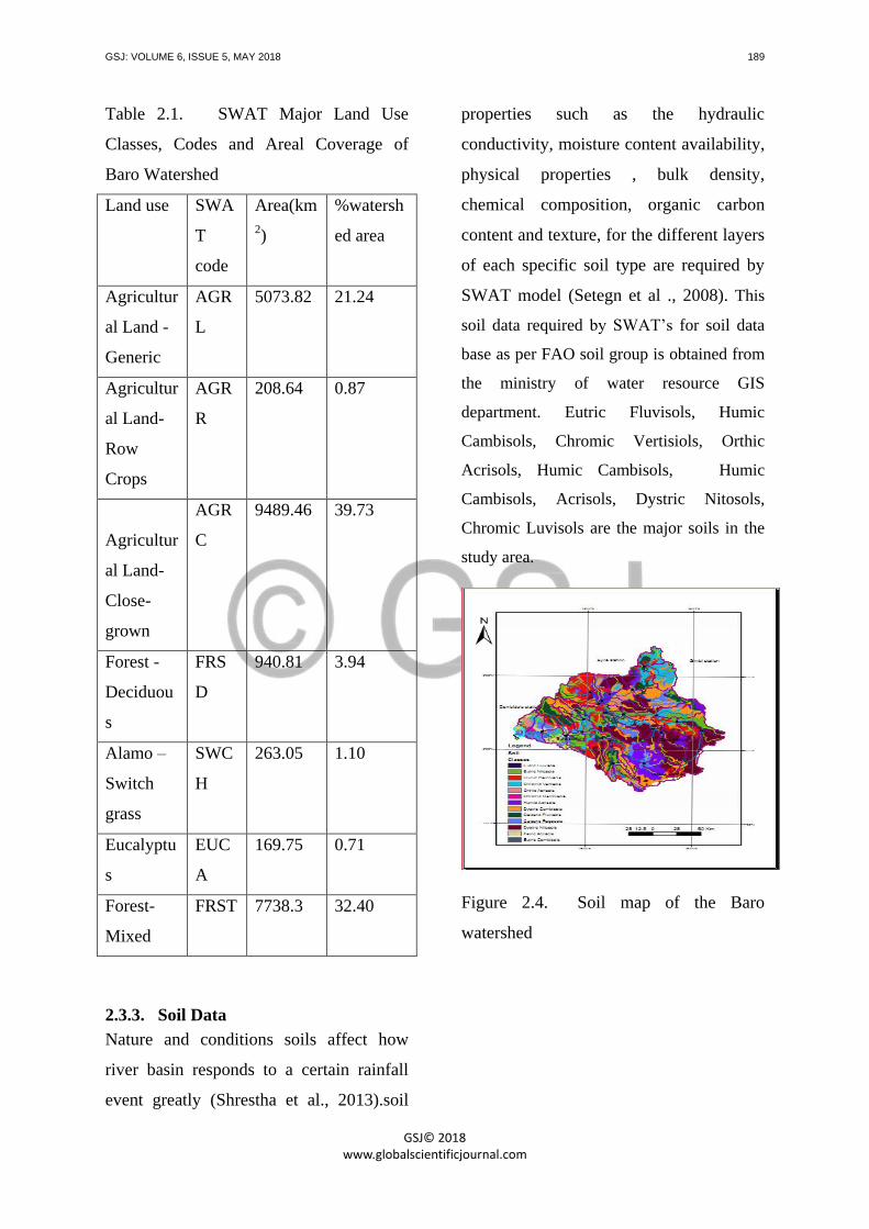
2.3.3. Soil Data

Nature and conditions soils affect how

river basin responds to a certain rainfall

event greatly (Shrestha et al., 2013).soil

properties such as the hydraulic

conductivity, moisture content availability,

physical properties , bulk density,

chemical composition, organic carbon

content and texture, for the different layers

of each specific soil type are required by

SWAT model (Setegn et al ., 2008). This

soil data required by SWAT’s for soil data

base as per FAO soil group is obtained from

the ministry of water resource GIS

department. Eutric Fluvisols, Humic

Cambisols, Chromic Vertisiols, Orthic

Acrisols, Humic Cambisols, Humic

Cambisols, Acrisols, Dystric Nitosols,

Chromic Luvisols are the major soils in the

study area.

Figure 2.4. Soil map of the Baro

watershed



Table 2.2.The SWAT result for the soils

area coverage in the watershed is shown

below.

Soil types Area (km2) % of total

area

Humic

Cambisols

2685.46 11.24

Eutric

Nitosols

1765.49 7.39

Orthic

cambisols

380.51 1.59

Chromic

vertisols

2392.12 10.02

Eutric

Cambisols

3940.13 8.58

Eutric

Fluvisols

1218.29 5.10

Orthic

Acrisols

2225.57 9.32

Chromic

Cambisols

4121.89 17.26

Dystric

Nitosols

7564.57 31.67

Ferric

Acrisols

530.44 2.22

2.3.4. Meteorological Data

To simulate the hydrological conditions of

the Basin meteorological data is needed by

the SWAT model. This meteorological

data required for the study were collected

from the Ethiopian National

Meteorological Services Agency (NMSA).

The meteorological data collected were

Precipitation, maximum and minimum

temperature, relative humidity, wind speed

and Sunshine hours. Data from twelve

stations, which are within and around the

study area, were collected. However, most

of the stations have short length of record

periods. Six of the stations have records

within the range of 1986-2016 but most of

them have missing data. The other

problem in the weather data was

inconsistency in the data record. In some

periods there is a record for precipitation

but there will be a missing data for

temperature, and vice versa.

Figure 2.5. Delineated Watershed of Baro

Watershed

Only Gore and Masha stations have data

for relative humidity, sunshine hours and

wind speed with short period of record. All

stations listed above contain daily rainfall

and temperature data for at least fifteen

years. Therefore all stations were used for

hydrological model development.



2.4 Hydrological data

The hydrological data was required for

performing sensitivity analysis, calibration

and Uncertainty analysis and validation of

the model. The hydrological data was also

collected from the Ethiopian Ministry of

Water, Irrigation and Electricity of

hydrological section. Even if the

hydrological data of daily flow was

collected for the rivers in the basin, due to

time limitation to accomplish sensitivity

analysis and calibration for the entire

basin, it was decided to concentrate on the

largest river Baro for modelling and

climate impact analysis. Hence, it was

only the hydrological data of the Baro used

for sensitivity analysis, calibration and

validation.

2.5 Hydro-Meteorological

Data Analysis

2.5.1. General

Hydrological modelling requires a hydro-

meteorological data (precipitation,

temperature, relative humidity and

sunshine hours) and hydrological (i.e

stream flow) data for analysis. But the

Reliability of the collected raw hydro-

meteorological and hydrological data

significantly affects quality of the model

input data and as a result, the model

simulation. Therefore the quality of the

data is directly proportional to the output

of the model at the of processing.

2.5.2. Missing Data Completion

Missing data is a common problem in the

hydrology. To perform hydrological

analysis and simulation using data of long

time series, filling in missing data is very

important. The missing data can be

completed using metrological and /or

hydrological stations located in the nearby,

provided that the stations are located in

hydrological homogeneous region.

Rainfall Data screening

Rough rainfall data screening of the six

meteorological stations in the study area

was first done by visual inspection of

monthly rainfall data. Because of long

braking in rainfall records of some stations

and absence of lengthy overlapping period

of record this inspection was done in the

record of the hydrologic years of 1986 to

2016 for thirty one years. Graphical

comparison of the rainfall data done by

creating time series plotting of monthly

rainfall data showed that the six stations

show similar periodic pattern.



Figure 2.6. Average Monthly Rainfall

data series (1986-2016)

When undertaking an analysis of

precipitation data from gauges where daily

observations are made, it is often to find

days when no observations are recorded at

one or more gauges. These missing days

may be isolated occurrences or extended

over long periods. In order to compute

precipitation totals and averages, one must

estimate the missing values. Several

approaches are used to estimate the

missing values. Station Average, Normal

Ratio, Inverse Distance Weighting, and

Regression methods are commonly used to

fill the missing records. In Station Average

Method, the missing record is computed as

the simple average of the values at the

nearby gauges. (Mc Cuen, 1998)

recommends using this method only when

the annual precipitation value at each of

the neighbouring gauges differs by less

than 10% from that for the gauge with

missing data.

]……….3.4.

Where:

Px= the missing precipitation record

P1, P2,..…..., Pm= precipitation records at

the neighbouring stations

M= Number of neighbouring stations

If the annual precipitations vary

considerably by more than 10 %, the

missing record is estimated by the Normal

Ratio Method, by weighing the

precipitation at the neighbouring stations

by the ratios of normal annual

precipitations.

………3.5.

Where:

Nx= Annual-average precipitation at the

gage with missing values

N1, N2,.…..., Nm= Annual average

precipitation at neighbouring gauges.

In this research because of the shortage of

the total annual rainfall and normal

rainfall, which is necessary conditions for

the normal ratio and station average

methods, the regression was good methods

of estimation to fill the gaps.

Method based on regression analysis

Assume that two precipitation gages Y and

X have long records of annual

precipitation, i.e.Y1, Y2,………,YN and

X1, X2,.…..XN. The precipitation Yt is

missing. We will fill in the missing data

based on a simple linear regression model.

The model can be written as:

Yt = a+bXt

Then R2 indicates the relationship between

the two variables. The higher the value of

R2

indicates the best fit of the regression

equation. Thus based on this for this

estimation different R-values are



calculated and the best fit selected for each

station. Based on this method all the

stations were filled and the regression

equations with basic parameters are shown

below.

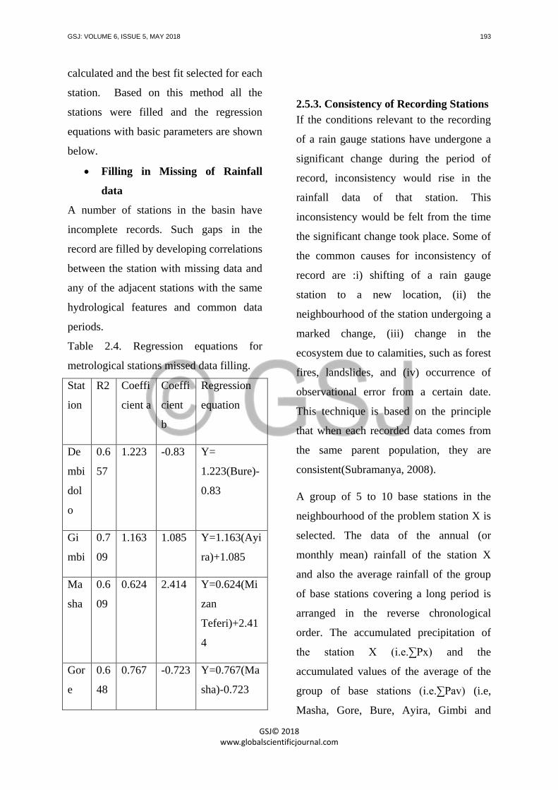
Filling in Missing of Rainfall

data

A number of stations in the basin have

incomplete records. Such gaps in the

record are filled by developing correlations

between the station with missing data and

any of the adjacent stations with the same

hydrological features and common data

periods.

Table 2.4. Regression equations for

metrological stations missed data filling.

Stat

ion

R2 Coeffi

cient a

Coeffi

cient

b

Regression

equation

De

mbi

dol

o

0.6

57

1.223 -0.83 Y=

1.223(Bure)-

0.83

Gi

mbi

0.7

09

1.163 1.085 Y=1.163(Ayi

ra)+1.085

Ma

sha

0.6

09

0.624 2.414 Y=0.624(Mi

zan

Teferi)+2.41

4

Gor

e

0.6

48

0.767 -0.723 Y=0.767(Ma

sha)-0.723

2.5.3. Consistency of Recording Stations

If the conditions relevant to the recording

of a rain gauge stations have undergone a

significant change during the period of

record, inconsistency would rise in the

rainfall data of that station. This

inconsistency would be felt from the time

the significant change took place. Some of

the common causes for inconsistency of

record are :i) shifting of a rain gauge

station to a new location, (ii) the

neighbourhood of the station undergoing a

marked change, (iii) change in the

ecosystem due to calamities, such as forest

fires, landslides, and (iv) occurrence of

observational error from a certain date.

This technique is based on the principle

that when each recorded data comes from

the same parent population, they are

consistent(Subramanya, 2008).

A group of 5 to 10 base stations in the

neighbourhood of the problem station X is

selected. The data of the annual (or

monthly mean) rainfall of the station X

and also the average rainfall of the group

of base stations covering a long period is

arranged in the reverse chronological

order. The accumulated precipitation of

the station X (i.e.∑Px) and the

accumulated values of the average of the

group of base stations (i.e.∑Pav) (i.e,

Masha, Gore, Bure, Ayira, Gimbi and



Dembi dolo stations) are calculated

starting from the latest record. Values of

∑Px are plotted against ∑Pav for various

consecutive time periods. If a decided

change in the regime of curve is observed

it should be corrected. However, as all the

selected stations in this study were

consistent as shown below by the double

mass curve there is no need of further

correction.



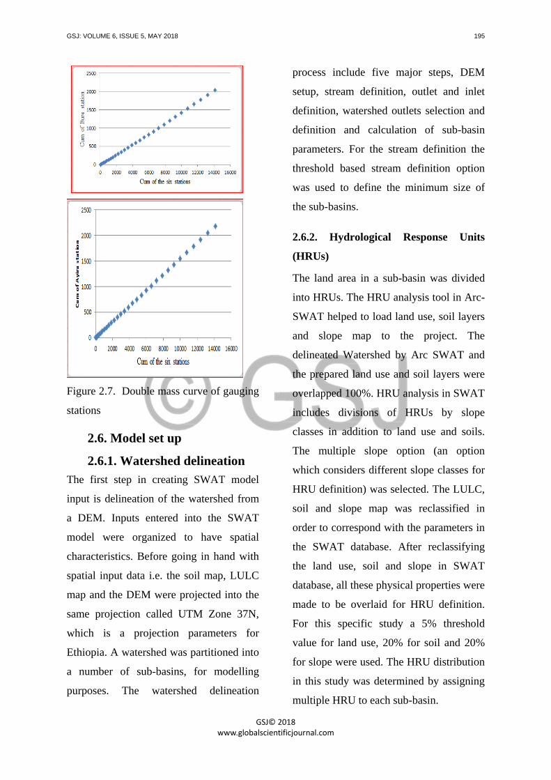
Figure 2.7. Double mass curve of gauging

stations

2.6. Model set up

2.6.1. Watershed delineation

The first step in creating SWAT model

input is delineation of the watershed from

a DEM. Inputs entered into the SWAT

model were organized to have spatial

characteristics. Before going in hand with

spatial input data i.e. the soil map, LULC

map and the DEM were projected into the

same projection called UTM Zone 37N,

which is a projection parameters for

Ethiopia. A watershed was partitioned into

a number of sub-basins, for modelling

purposes. The watershed delineation

process include five major steps, DEM

setup, stream definition, outlet and inlet

definition, watershed outlets selection and

definition and calculation of sub-basin

parameters. For the stream definition the

threshold based stream definition option

was used to define the minimum size of

the sub-basins.

2.6.2. Hydrological Response Units

(HRUs)

The land area in a sub-basin was divided

into HRUs. The HRU analysis tool in Arc-

SWAT helped to load land use, soil layers

and slope map to the project. The

delineated Watershed by Arc SWAT and

the prepared land use and soil layers were

overlapped 100%. HRU analysis in SWAT

includes divisions of HRUs by slope

classes in addition to land use and soils.

The multiple slope option (an option

which considers different slope classes for

HRU definition) was selected. The LULC,

soil and slope map was reclassified in

order to correspond with the parameters in

the SWAT database. After reclassifying

the land use, soil and slope in SWAT

database, all these physical properties were

made to be overlaid for HRU definition.

For this specific study a 5% threshold

value for land use, 20% for soil and 20%

for slope were used. The HRU distribution

in this study was determined by assigning

multiple HRU to each sub-basin.



2.6.3. Weather Generation

The swat model has an automatic weather

data generator. However it needs some

input data to run the model. Input data

required are daily values of precipitation,

maximum and minimum temperature,

solar radiation, wind speed and relative

humidity. But, in many areas such data are

either incomplete or records may not have

sufficient length, which is the case in this

study. If no data are available at the same

time for all stations, the model can

generate all the remaining data from daily

precipitation and temperature data. In this

research of the six stations which were

used in order to run the SWAT model only

two stations have full data. These stations

are Masha and Gore meteorological

stations. Using these two stations the

SWAT model generates representative

weather variables for Baro watershed. In

this research, six stations were used to run

the swat model for estimation of surface

runoff. From this six stations only two of

them are with full of data (i.e Gore and

Masha stations) .Therefore from this two

stations weather is generated for the rest of

missing stations using the automatic

weather data generator.

2.6.4. Sensitivity analysis

Sensitivity analysis is a technique of

identifying the responsiveness of different

parameter involving in the simulation of a

hydrological process. For big hydrological

models like SWAT, which involves a wide

range of data and parameters in the

simulation process, calibration is quite a

bulky task. Even though, it is quite clear

that the flow is largely affected by curve

number, for example in the case of SCS

curve number method, this is not sufficient

enough to make calibration as little change

in other parameters could also change the

volumetric, spatial, and temporal trend of

the simulated flow. Hence, sensitivity

analysis is a method of minimizing the

number of parameters to be used in the

calibration step by making use of the most

sensitive parameters largely controlling the

behaviour of the simulated process

(Zeray., 2006). This appreciably eases the

overall calibration and validation process

as well as reduces the time required for it.

After a thorough pre-processing of the

required input for SWAT 2012 model,

flow simulation was performed for a thirty

one years of recording periods starting

from 1986 through 2016.The first four

years of which was used as a warm up

period and the simulation was then used

for sensitivity analysis of hydrologic

parameters and for calibration of the



model. Sensitivity analysis was performed

on 19 SWAT parameters and the most

sensitive parameters were identified using

Global sensitivity analysis method in

SWAT-CUP SUFI12. (Griensven.A,

2005).

2.6.5. Calibration and Validation of

SWAT Model

SWAT-CUP

SWAT-CUP is an interface that was

developed for SWAT. Using this generic

interface, any calibration/uncertainty or

sensitivity program can easily be liked to

SWAT.

Calibration of Model

Calibration is the process whereby model

parameters are adjusted to make the model

output match with observed data. There

are three calibration approaches widely

used by the scientific community. These

are the manual calibration, automatic

calibration and a combination of the two.

Automated model calibration requires that

the uncertain model parameters are

systematically changed, the model is run,

and the required outputs (corresponding to

measured data) are extracted from the

model output files.

The main function of an interface is to

provide a link between the input/output of

a calibration program and the model. The

simplest way of handling the file exchange

is through text file formats.

The manual calibration approach requires

the user to compare measured and

simulated values, and then to use expert

judgment to determine which variables to

adjust, how much to adjust them, and

ultimately assess when reasonable results

have been obtained (Gassman, 2005)

presented nearly 20 different statistical

tests that can be used for evaluating

SWAT stream flow output during a

manual calibration process. They

recommended using the Nash-Suttcliffe

simulation efficiency ENS and regression

coefficients R2 for analysing monthly

output, based on comparisons of SWAT

stream flow results with measured stream

flows for the same watershed.

Validation of Model

Calibrated model parameters can result in

simulations that satisfy goodness-of fit

criteria, but parameter values may not have

any hydrological meaning. Values of

model parameters will be a result of curve

fitting. This is also reflected in having

different sets of parameter values

producing simulations, which satisfy these

criteria. It is necessary to test if parameter

values reflect the underlying hydrological

processes, and are not a result of curve

fitting. Therefore; to conduct appropriate

model validation results, it is necessary to



carry out split sample test. The split-

sample test involves splitting the available

time series into two parts. One part is used

to calibrate the model, and the second part

is used for testing (validating) if calibrated

parameters can produce simulations, which

satisfy goodness-of-fit tests.

The spilt sample test is suitable for

catchments with long time series, and it is

applied in this catchment since it has thirty

one years of data. For this catchment, the

available record is split into two equal

parts that is from 1990-2005 for

calibration and 2006-2016 for validation.

2.6.6. SWAT-Model Performance

Assessment

To evaluate the model performance a

coefficient of determination (R2), Nash-

Sutcliffe (NSE), and root mean square

error (RMSE) are applied. The accuracy of

the simulated value when compared with

the observed value is evaluated by R2,

whereas the NSE measures the goodness

of fit and describes the variance between

the simulated and observed values. It

depicts the strength between the simulated

and observed data and the direction of the

linear relation. (X.Zhang, 2007).

Generally, the calibration and validation of

the SWAT model are considered to be

acceptable or satisfactory performance

when NSE is within the range of 0.5 and

0.65, considered satisfactory when the

range is between 0.65 and 0.75.The NSE

value between 0.75 and 1.00 indicate a

very good performance. Lastly, RMSE

was used to assess the validity of the

model in this study. The desired value for

RMSE is 0, which depicts a perfect

simulation, with lower values representing

better performance.

Table 3.5. General Performance rating for

the recommended statistics

Performance

Rating

NSE

Very good 0.75<NSE≤1.00

Good 0.65<NSE≤0.75

Satisfactory 0.50<NSE≤0.65

Unsatisfactory NSE≤ 0.50

2.7. Climate Change Scenarios

When attempting to evaluate the response

or sensitivity of any physical (or

biological) system to climate change, one

of the largest uncertainties introduced is

our current level of understanding (or lack

thereof) of the magnitude, or even the

direction of future climate change. Even if

global climate change could be modeled

using today's general circulation models

(GCMs), much climatic variation takes

place at regional and smaller scales that

are unresolved and will remain so for the

foreseeable future. Because of this, studies

of the effects of climate change on

hydrologic systems are limited to the use



of climate change scenarios that may or

may not match future climate realities.

However, these scenarios are useful for

investigating the response of hydrologic

systems to climate change and variability

since they are easily constructed and

employed as inputs to other models.

A number of different approaches to

developing climate change scenarios have

been devised in recent years. These

include GCM output, analog climates

(historical, paleoclimatic or spatial),

synthesis scenarios ("scenarios by

committee"), arbitrary change scenarios, or

scenarios based on physical or statistical

arguments (WMO, 1987) . While GCM

output can provide some indication of the

direction as well as the possible magnitude

of a climate change associated with some

forcing (e.g., doubled CO2), the

uncertainties associated with GCMs, as

well as their poor spatial resolution, reduce

their usefulness for studies of regional

hydrologic consequences of climate

change. Although resource managers and

planners may desire indications of climate

change direction and magnitude, GCM

output must be used cautiously.

Hypothetical, arbitrary climate change

scenarios can be developed at much lower

cost than GCM scenarios, and can provide

useful information on the response of

hydrologic systems to plausible levels of

climate change and variability.

Only two climatic inputs (temperature and

precipitation) were used to compute the

climate change impact on the Hydrology

of the Baro Catchment. Scenarios with

mean annual temperature changes of 0oC,

2oC, 3.5

oC, 4.5

oC, 6

oC and annual total

precipitation changes from -20% to +20%

at 10% interval were constructed with the

assumption that all months experienced the

same change (i.e constant temperature

change or precipitation change.

2.7.1. Impact of climate change on

Water yields

By adjusting the climatic inputs in the

SWAT model, impact assessment of

climate change on water yields can be

accomplished. Simulated water yields

under the High future scenarios RCP8.5

were evaluated relative to the observed

monthly discharge for the gauge station

Baro watershed. This was done through

graphical methods. Regression graphs of

the annual totals of the observed for the

period 1986- 2016 were compared with

those of the simulated water yields for the

2050s and 2080s from the two climate

change scenarios (i.e. precipitation and

temperature change scenarios).



3. Result and Discussion

3.1. SWAT Hydrological Model

Results

3.1.1. Watershed Delineation

The Arc SWAT interface proposes the

minimum, maximum, and suggested size

of the sub basin area (in hectare) to define

the minimum drainage area required to

form the origin of a stream. Generally, the

smaller the threshold area, the more

detailed are the drainage networks, and the

larger are the number of sub-basins and

HRUs. However, this needs more

processing time and space. As a result, an

optimum size of a watershed that

compromises both was selected.

(Dilnesaw, 2006) did a sensitivity analysis

of the threshold area on SWAT model

performance and found that the optimum

threshold area that can be used for the

delineation procedure is ±1/3 of the

suggested threshold area. Therefore, a

threshold area of -1/3 of that suggested by

the model was used.

After running the SWAT model to find the

climate impact on the Baro River and

SWAT-CUP for calibration of the model,

the following results were found. The

average annual rainfall of the basin is

2156.8 mm and surface water runoff of

891.09 mm and lateral soil flow is 57.77

mm. The entire model output types, which

have monthly and annual values is shown

in table 5.1. The total runoff found by the

model in the Catchment area of 24563.64

km2.

Table 3.1 Average annual basin values.

AVERAGE ANNUAL BASIN VALUE

Precipitation 2156.8mm

Surface runoff Q 891.09mm

Lateral Soil Q 57.77mm

Ground water (shal

AQ) Q

580.08mm

Groundwater (Deep

AQ)Q

47.1mm

Revap (Shal AQ

soil/plants)

24.1mm

Deep AQ recharge 29.00mm

Total AQ recharge 954.36

Total water yield 1223.06mm

Percolation out of

soil

935.17mm

ET 627.2mm

PET 1204.9mm

Table 3.2. Average Monthly Basin Values

.

MO

N

RAI

N

SU

RF

Q

LA

T Q

Water

Yiled

ET PE

T

mm mm mm mm mm mm mm

1 29.

54

0.5

9

1.3

1

17.93 24.

14

115

.77

2 25.

26

0.4

2

1.0

1

11.6 39.

2

121

.99

3 130

.53

55.

33

1.4

7

63.51 71.

23

133

.59

4 102 2.0 2.4 15.13 72. 121



.89 6 6 56 .06

5 299

.46

89.

86

4.6

5

114.0

8

68.

78

102

.46

6 240

.79

8.6

4

7.0

5

85.81 61.

06

76.

08

7 370

.29

119

.97

8.5

9

218.2 56.

85

70.

74

8 414

.63

157

.83

9.4 290.1

2

58.

62

76.

63

9 280

.07

52.

44

8.8

6

176.6

1

57.

01

81.

18

10 174

.73

17.

95

7.6 125.9

7

54.

64

96.

52

11 61.

67

2.3

6

4.1

4

69.28 41.

35

99.

99

12 27.

4

0.7

2

2.1

8

35.05 29.

28

112

.04

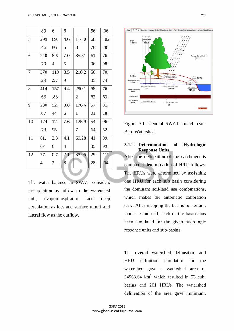
The water balance in SWAT considers

precipitation as inflow to the watershed

unit, evapotranspiration and deep

percolation as loss and surface runoff and

lateral flow as the outflow.

Figure 3.1. General SWAT model result

Baro Watershed

3.1.2. Determination of Hydrologic

Response Units

After the delineation of the catchment is

completed determination of HRU follows.

The HRUs were determined by assigning

one HRU for each sub basin considering

the dominant soil/land use combinations,

which makes the automatic calibration

easy. After mapping the basins for terrain,

land use and soil, each of the basins has

been simulated for the given hydrologic

response units and sub-basins

The overall watershed delineation and

HRU definition simulation in the

watershed gave a watershed area of

24563.64 km2 which resulted in 53 sub-

basins and 201 HRUs. The watershed

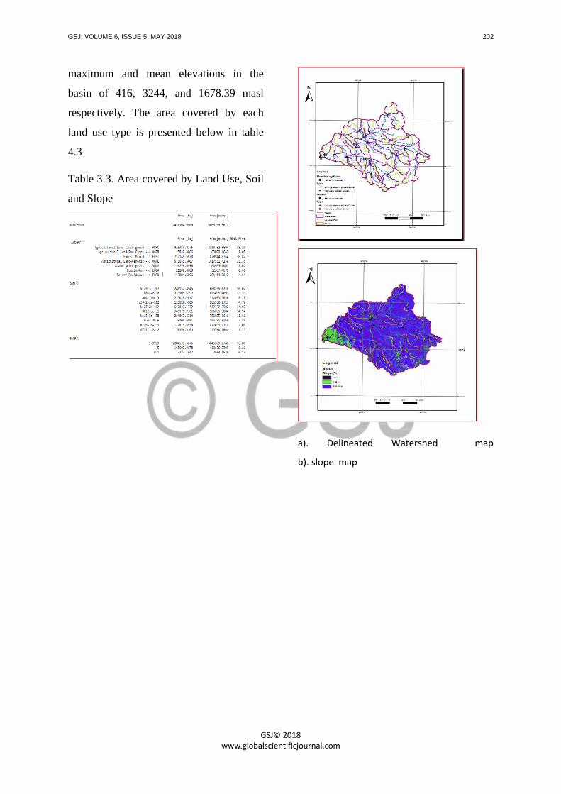
delineation of the area gave minimum,



maximum and mean elevations in the

basin of 416, 3244, and 1678.39 masl

respectively. The area covered by each

land use type is presented below in table

4.3

Table 3.3. Area covered by Land Use, Soil

and Slope

a). Delineated Watershed map

b). slope map



a) Land use map

d) soil map

Figure 3.2. The delineated sub basins, land

use, slope, and soil map of the Baro-

Watershed

3.2. Performance Evaluation of

the Hydrologic Model

3.2.1. Sensitivity Analysis

Sensitivity analysis is the process of

identifying the model parameters that exert

the highest influence on model calibration

or on model predictions. Even though 19

parameters were used for the sensitivity

analysis, all of them have no meaningful

effect on the daily flow of the Baro River.

Table 4.5 below shows the rank of

sensitive parameters according to their

effect on the catchment.

Nineteen hydrological model parameters

of the SWAT model underwent sensitivity

and uncertainty analyses using Global

sensitivity analysis method in SWAT-CUP

SUFI2. The top 12 parameters having

sensitivity indices greater than or equal to

0.05 were then selected, as shown in table

below.

moisture condition II (CN2)

base flow alpha factor (Alpha_Bf)

Available water capacity of the soil

layer (SOL-AWC)

Groundwater “revap” coefficient,

(GW-REVAP)

Manning’s n value for main

channel (CH-N2)

Threshold depth of water in the

shallow aquifer for return flow to

occur (mm) (GWQMN)



Surface Runoff Lag time

(SURLAG)

Plant uptake compensation factor

(EPCO)

Depth from soil surface to bottom

of layer (SOL_Z)

Channel effective hydraulic

conductivity (CH_K2)

Soil Evaporation compensation

factor (ESCO)

Manning’s “n” value for overland

flow (OV_N)

Threshold depth of water in the

shallow aquifer required for return

flow to occur (mm)

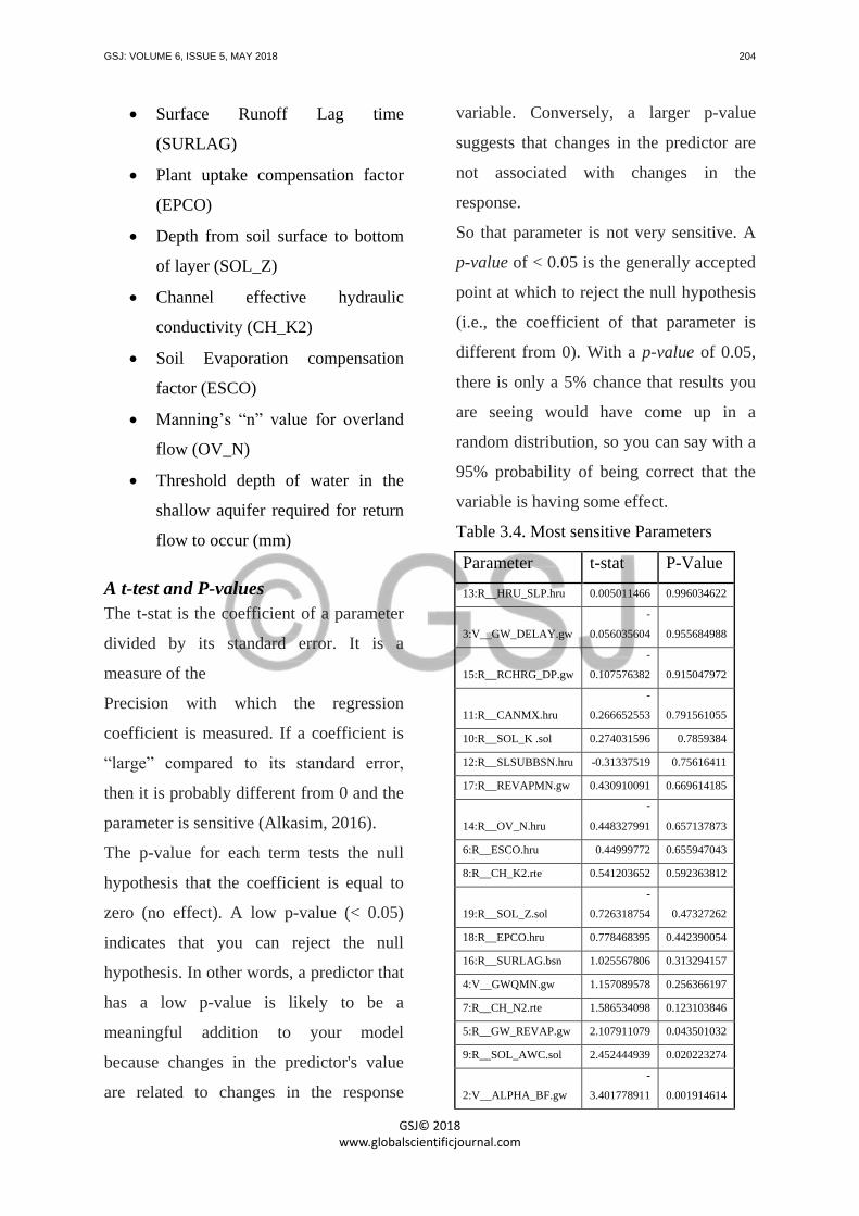
A t-test and P-values

The t-stat is the coefficient of a parameter

divided by its standard error. It is a

measure of the

Precision with which the regression

coefficient is measured. If a coefficient is

“large” compared to its standard error,

then it is probably different from 0 and the

parameter is sensitive (Alkasim, 2016).

The p-value for each term tests the null

hypothesis that the coefficient is equal to

zero (no effect). A low p-value (< 0.05)

indicates that you can reject the null

hypothesis. In other words, a predictor that

has a low p-value is likely to be a

meaningful addition to your model

because changes in the predictor's value

are related to changes in the response

variable. Conversely, a larger p-value

suggests that changes in the predictor are

not associated with changes in the

response.

So that parameter is not very sensitive. A

p-value of < 0.05 is the generally accepted

point at which to reject the null hypothesis

(i.e., the coefficient of that parameter is

different from 0). With a p-value of 0.05,

there is only a 5% chance that results you

are seeing would have come up in a

random distribution, so you can say with a

95% probability of being correct that the

variable is having some effect.

Table 3.4. Most sensitive Parameters

Parameter t-stat P-Value

13:R__HRU_SLP.hru 0.005011466 0.996034622

3:V__GW_DELAY.gw

-

0.056035604 0.955684988

15:R__RCHRG_DP.gw

-

0.107576382 0.915047972

11:R__CANMX.hru

-

0.266652553 0.791561055

10:R__SOL_K .sol 0.274031596 0.7859384

12:R__SLSUBBSN.hru -0.31337519 0.75616411

17:R__REVAPMN.gw 0.430910091 0.669614185

14:R__OV_N.hru

-

0.448327991 0.657137873

6:R__ESCO.hru 0.44999772 0.655947043

8:R__CH_K2.rte 0.541203652 0.592363812

19:R__SOL_Z.sol

-

0.726318754 0.47327262

18:R__EPCO.hru 0.778468395 0.442390054

16:R__SURLAG.bsn 1.025567806 0.313294157

4:V__GWQMN.gw 1.157089578 0.256366197

7:R__CH_N2.rte 1.586534098 0.123103846

5:R__GW_REVAP.gw 2.107911079 0.043501032

9:R__SOL_AWC.sol 2.452444939 0.020223274

2:V__ALPHA_BF.gw

-

3.401778911 0.001914614



1:R__CN2.mgt 5.151955794 0.000015167

Based on A t-test that was used to identify

the relative significance of each parameter

that was a value larger in absolute value

was most significant and p-value the

significance of the sensitivity, a value

close to zero is more significant. From the

model output, the first two most sensitive

parameters are SCS runoff curve number f

(CN2) and base flow alpha factor

(Alpha_Bf).

3.2.2. Model Calibration

The calibration of the model was

performed for 16 years (1990 to 2005)

using Baro River flow data at Gambella

gauging station. Taking the first four years

as a warm up period, the flow was

simulated for 16 years from January 1st

1990 to December 31st 2005.

The automatic calibration SUFI-2 was

used to calibrate the model using the

observed stream flow. Observed daily

stream flows were adjusted on the monthly

basis and simulations run were conducted

on monthly basis to compare the modeling

output with the measured daily discharge

at the outlet of Baro watershed.

Table 3.5. Model efficiencies parameters

in calibration and validation periods

Sub

basin No

Simulatio

n period

Paramet

er

period value

s

6

gauging

stations

1990-

2005

R2 Calibr

ation

0.9

NS Calibr

ation

0.66

2006-

2016

R2 Valid

ation

0.93

NS Valid

ation

0.61

Figure 3.3. Calibration results of average

monthly simulated and observed flows of

Baro River at Gambella station (1990-

2005)



Figure 3.4. Simulated and observed flows

during the calibration period using scatter

plot (1990-2005)

3.2.3. Model Validation

Model validation was carried out over the

period of 2006-2016. As it can be seen in

figure below the model performance is

improved, the coefficient of determination

in this case is found to be R2=0.93 and

NSE=0.61. The observed and simulated

flow hydrograph show well agreement. In

general the model performed reasonably in

simulating flows for periods outside of the

calibration period, based on adjusted

parameters during calibration.

Figure 3.5. Validation results of average

monthly flows of Baro at Gambella station

(2006-2016).

Figure 3.6. Observed vs simulated flow

for validation (2006-2016).

3.3. Scenarios Developed for the

Future

Warming projections under medium

scenarios indicate that extensive areas of

Africa will exceed 2oC by the last two

decades of this century relative to the late

20th

century mean annual temperature and

all of Africa under high emission scenarios

(RCP 8.5 W/m2) and reach between 3

oC

and 6oC by the end of this century (Niang,

2014).

Most of areas of the African continent lack

sufficient observational data to draw

conclusions about trends in annual

precipitation over the past century. In

addition to this, in many regions of the

continent differences exist between

different observed precipitation data sets

(Nikilin, 2012). Therefore to check simply

the effect of precipitation change on the

stream flow, precipitation variation of

from -20% to +20% was taken.

The changes in stream flow under the

impact of climate change was investigated



by using several hypothetical scenarios

(synthetic approach) applied to the climate

normal (1986-2016) meteorological data.

Incremental climate change scenarios were

applied with a hypothetical temperature

increase (0, +2oC, +3

oC, +4

oC, +5

oC and

+6oC) and precipitation change from -20%

to +20% at 10% interval were examined to

check the impact of climate change in the

stream flow. In this research the impact

were analyzed for 2050s with temperature

change of 0oC, 2

oC, 3

oC and for 2080s

with temperature change of 4oC, 5

oC and

6oC.

For a constant temperature the total annual

water yield increases with the increment of

Precipitation as it is shown in the Figure

4.10. On the other hand for constant

precipitation the average water yield

decreases with the increment of

temperature in the stream flow for the

period of 2050s and 2080s as shown in

Figure 4.9. For example for temperature of

0oC but with increment of precipitation the

average water yield will increase as shown

below in the table below whereas for

constant precipitation there is a reduction

of total water yield.

Table 3.6. Total annual water yield for

the 2050s and 2080s

ΔP -20% -10% 0% 10% 20%

0oC 1521.05 1523.13 1525.11 1527.29 1529.37

2oC 1498.63 1500.7 1502.77 1504.84 1506.91

ΔT 3oC 1485.46 1487.52 1489.59 1491.65 1493.71

4oC 1472.52 1474.58 1476.63 1478.69 1480.74

5oC 1459.75 1461.79 1463.84 1465.84 1467.94

6oC 1446.82 1448.86 1450.49 1452.94 1454.98

Figure 3.7: Trend which shows the

variation of total annual water yield for

constant precipitation but with varying

temperature

Figure 3.8: Trend which shows the

variation of total annual water yield for

constant precipitation but with varying

temperature

3.3.1. Sensitivity Analysis

The changes in stream flow under the

impact of climate change was investigated

by using several hypothetical scenarios

(synthetic approach) applied to the climate

normal (1986-2016) meteorological data.

Incremental climate change scenarios were



applied with a hypothetical temperature

increase of 0oC, 2

oC and 3

oC for the period

of 2050s according to IPCC Fifth

Assessment report set for Africa and 4oC,

5oC and 6

oC for the period of 2080s. On

the other hand taking the precipitation

range from -20% to 20% at 10% interval

the change of the flow is examined as

shown below.

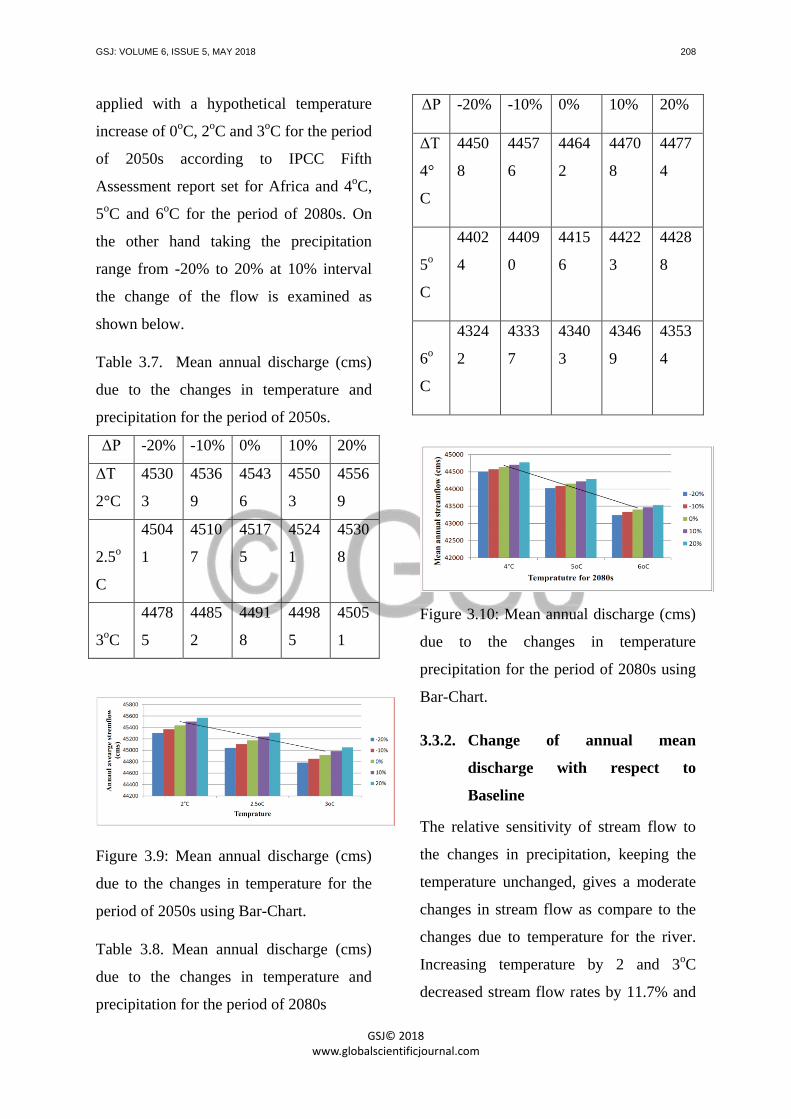
Table 3.7. Mean annual discharge (cms)

due to the changes in temperature and

precipitation for the period of 2050s.

ΔP -20% -10% 0% 10% 20%

ΔT

2°C

4530

3

4536

9

4543

6

4550

3

4556

9

2.5o

C

4504

1

4510

7

4517

5

4524

1

4530

8

3oC

4478

5

4485

2

4491

8

4498

5

4505

1

Figure 3.9: Mean annual discharge (cms)

due to the changes in temperature for the

period of 2050s using Bar-Chart.

Table 3.8. Mean annual discharge (cms)

due to the changes in temperature and

precipitation for the period of 2080s

ΔP -20% -10% 0% 10% 20%

ΔT

4°

C

4450

8

4457

6

4464

2

4470

8

4477

4

5o

C

4402

4

4409

0

4415

6

4422

3

4428

8

6o

C

4324

2

4333

7

4340

3

4346

9

4353

4

Figure 3.10: Mean annual discharge (cms)

due to the changes in temperature

precipitation for the period of 2080s using

Bar-Chart.

3.3.2. Change of annual mean

discharge with respect to

Baseline

The relative sensitivity of stream flow to

the changes in precipitation, keeping the

temperature unchanged, gives a moderate

changes in stream flow as compare to the

changes due to temperature for the river.

Increasing temperature by 2 and 3oC

decreased stream flow rates by 11.7% and



12.73%, respectively, while 10% and 20%

drop in rainfall resulted in a stream flow

decrease of 11.6% and 11.7%. These result

suggested that stream flow in the Baro

Watershed will be more sensitive to the

average increase in temperature than to the

average decrease in rainfall, showing the

role of evapotranspiration in the water

cycle.

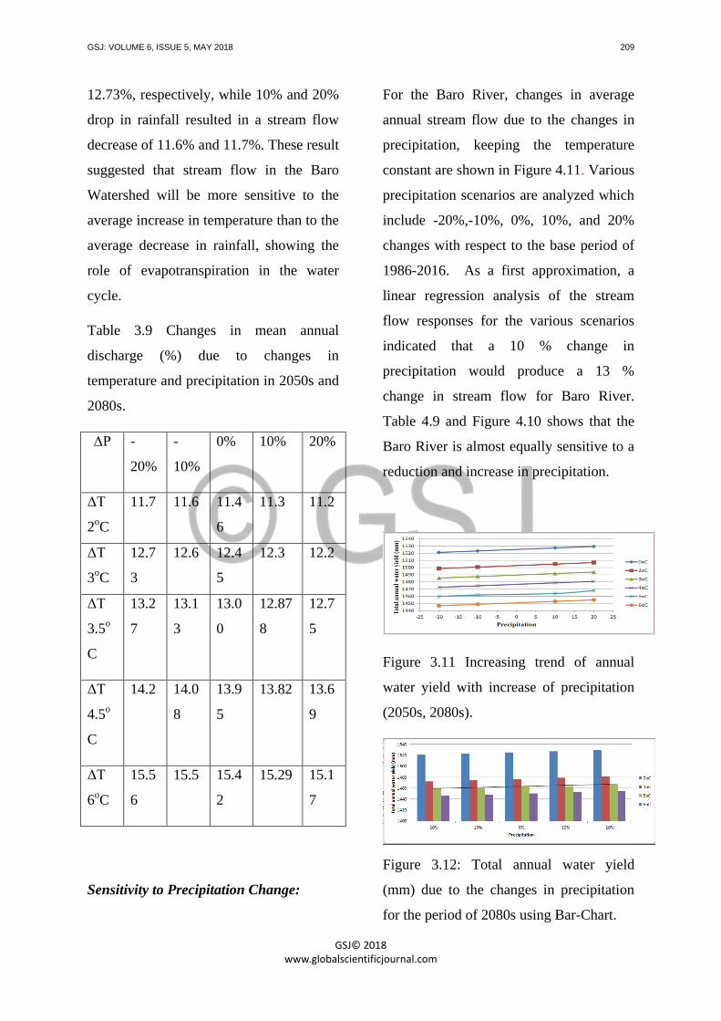
Table 3.9 Changes in mean annual

discharge (%) due to changes in

temperature and precipitation in 2050s and

2080s.

ΔP -

20%

-

10%

0% 10% 20%

ΔT

2oC

11.7 11.6 11.4

6

11.3 11.2

ΔT

3oC

12.7

3

12.6 12.4

5

12.3 12.2

ΔT

3.5o

C

13.2

7

13.1

3

13.0

0

12.87

8

12.7

5

ΔT

4.5o

C

14.2 14.0

8

13.9

5

13.82 13.6

9

ΔT

6oC

15.5

6

15.5 15.4

2

15.29 15.1

7

Sensitivity to Precipitation Change:

For the Baro River, changes in average

annual stream flow due to the changes in

precipitation, keeping the temperature

constant are shown in Figure 4.11. Various

precipitation scenarios are analyzed which

include -20%,-10%, 0%, 10%, and 20%

changes with respect to the base period of

1986-2016. As a first approximation, a

linear regression analysis of the stream

flow responses for the various scenarios

indicated that a 10 % change in

precipitation would produce a 13 %

change in stream flow for Baro River.

Table 4.9 and Figure 4.10 shows that the

Baro River is almost equally sensitive to a

reduction and increase in precipitation.

Figure 3.11 Increasing trend of annual

water yield with increase of precipitation

(2050s, 2080s).

Figure 3.12: Total annual water yield

(mm) due to the changes in precipitation

for the period of 2080s using Bar-Chart.



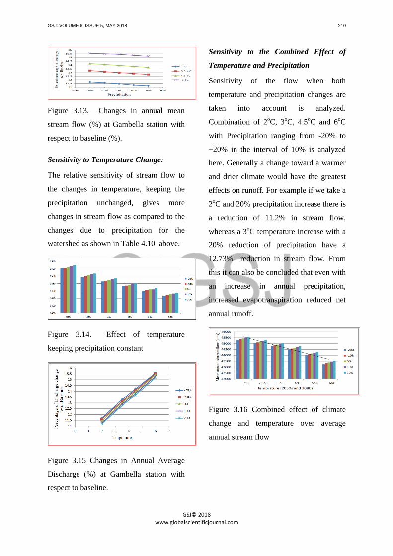
Figure 3.13. Changes in annual mean

stream flow (%) at Gambella station with

respect to baseline (%).

Sensitivity to Temperature Change:

The relative sensitivity of stream flow to

the changes in temperature, keeping the

precipitation unchanged, gives more

changes in stream flow as compared to the

changes due to precipitation for the

watershed as shown in Table 4.10 above.

Figure 3.14. Effect of temperature

keeping precipitation constant

Figure 3.15 Changes in Annual Average

Discharge (%) at Gambella station with

respect to baseline.

Sensitivity to the Combined Effect of

Temperature and Precipitation

Sensitivity of the flow when both

temperature and precipitation changes are

taken into account is analyzed.

Combination of 2oC, 3

oC, 4.5

oC and 6

oC

with Precipitation ranging from -20% to

+20% in the interval of 10% is analyzed

here. Generally a change toward a warmer

and drier climate would have the greatest

effects on runoff. For example if we take a

2oC and 20% precipitation increase there is

a reduction of 11.2% in stream flow,

whereas a 3oC temperature increase with a

20% reduction of precipitation have a

12.73% reduction in stream flow. From

this it can also be concluded that even with

an increase in annual precipitation,

increased evapotranspiration reduced net

annual runoff.

Figure 3.16 Combined effect of climate

change and temperature over average

annual stream flow



Figure 3.17 Combined effects of climate

change and temperature over average

annual stream flow.

4. Conclusion and Recommendation

4.1. Conclusion

In this study, potential impacts of climate

change on the future stream flow of the

Baro River has been assessed by using

SWAT hydrological model on the basis of

climate change forced by RCP 8.5

scenarios of IPCC 5th

Assessment (AR5)

report for 2050s and 2080s.

The SWAT model was used to create a

hydrological model on the Baro watershed

to investigate the effect of climate

sensitivity on the stream flow based on the

basis of climate change scenarios projected

by IPCC 5th

Assessment (AR5) report for

2050s and 2080s of the 21st century for

African countries. This special Thesis

focuses on the worst condition of RCP

8.5W/m2

by taking the scenarios of

temperature change and precipitation

according to the IPC report set for African

countries. For a region with critical water

needs, understanding the possible

consequences of climate change on stream

flow is necessary to ensure adequate future

supplies.

Initially the calibration and validation of

the stream flow was made in which for the

calibration the period from 1990-2005 was

taken and for the validation process the

period from 2005-2016 was taken. From

the result a good performance was found

with R2 and NSE greater than 0.6 and 0.5

respectively. Following to the calibration

and validation, the SWAT model was re-

run using the temperature and precipitation

scenarios to predict the impact of climate

changes on the stream flow of the river.

Then sensitivity of the flow to temperature

and precipitation change at the Baro River

in Gambella station was assessed.

This work demonstrated the high

vulnerability of stream flow to changes in

temperature and rainfall in the catchment.

Generally, the decrease in rainfall was

accompanied by a large increase in the

evapotranspiration. The combination of

this two trend is likely to result in

decreased availability of water. A decrease

in stream flow of 12.73% and 15.56% is

expected for the period of 2050s and

2080s.

Precipitation scenarios yielded stream

flow variations that correspond to the

change of rainfall intensity and amount of

rainfall, while scenarios with increased air



temperature yielded a decrease in water

level leading to a water shortage. Change

in Temperature had a large effect on the

magnitude of seasonal annual runoff than

temperature.

4.2. Recommendation

The results of this study is a basis for

informed decision in the water sector in

terms of short and long term

implementation of development projects

and also strategic planning policies. These

results can also be used in the water sector

for water resources management and

disaster risk reduction.

The results can be used by policy makers

in understanding the vulnerability level of

the Baro Catchment to climate change

impacts; this will help in coming with

suitable mitigation and adaptation

approaches.

In the present research scenarios with

mean annual temperature changes and

annual total precipitation changes were

constructed with the assumption that all

months experienced the same change (i.e.

constant temperature change or percentage

precipitation change). While not all of the

resulting scenarios are equally likely, and

real climate changes will undoubtedly

affect the seasonal cycle as well as the

mean climate, these scenarios offer a

simple basis on which to evaluate the

impacts of climate change and variability

on stream flow. Therefore it is

recommended for the next researcher to

include the seasonal effect of climate on

the stream flow so that one can provide a

good insight to the effect of climate

change on the stream flow.

In the present study the land use was take

for one year at the beginning of 21st

century , for better approximation of future

projected flow land use/land cover changes

and population increase that cause

difference in the water availability can be

included in this model .

REFERENCE

Abbaspour et al. K.C., Yang, I.Maimov,

R.Siber, K.Bogner, J.Mieleitner, J.Zobrist,

R.Srinivasan Modeling hydrology and water

quality in the pre-alpine/alpine Thur

watershed using SWAT [Journal] //

hydrology. - 2007. - pp. 413-430.

Abera F.F. Assessment of climate change

impact on the hydrology of upper guder

catchment , Upper Blue Nile [Journal]. - Addis

Ababa : [s.n.], 2011.

Alam Sarfaraz Impact of climate change on

future flow of Brahmaputra rievr basin using

SWAT Model [Journal]. - Dhaka : [s.n.], 2015.



Alkasim Mohammed Assessment and

evaluation of surface water potential and

demands in Baro-Akobo River Basin, Ethiopia

[Journal]. - Addis Ababa : [s.n.], 2016.

Allen et al. V.R.B., John broom climate

change synthesis report. IPCC Fifth

asessement report [Journal]. - 2014.

Arnell Climate change and global water

resources [Journal]. - 1999. - Vol. 9.

Arnold Automated base flow separation and

recession analysis techniques [Journal] //

Groundwater. - 2009. - p. 33(6).

Arnold et al., Automatde base flow

separation and recession analysis techniques

[Journal]. - 1998. - Vol. 6.

Bates S.Wu and J.P.Palutikof climate change

and water, technical paper of the

intergovernmental panle on climate change

[Journal]. - Geneva : [s.n.], 2008.

Baven K. J.Freer, Equifinality, data

assimilation and uncertainity estimation in

mechanistic modelling of complex

environmental syatems using the GLUE

methodology [Journal] // Journal of

Hydrology. - 2001. - pp. 11-29.

Berhane Mesgana Estimation of Monthly

Flow for Ungauged Catchment (case study of

Baro-Akobo basin) [Journal]. - Addis Ababa :

[s.n.], 2013.

Chong-yu Xu from GCMs to river flow: a

review of downscaling methods and

hydrologic modeling approaches [Report]. -

Uppsala, Sweden : [s.n.], 1999.

Di Baldassarre G Elshamy M, van Griensven,

A Soliman E Kigobe M Future Hydrology and

climate in the River Nile basin [Report]. -

2011.

Dilnesaw A. Modelling of Hydrology and Soil

Erosion of Upper Awash River Basin, PHD

Thesis [Report]. - Bonn : [s.n.], 2006.

Ebi et al. K.L., Hallegatte, S., Kram, T., Arnell,

N.W., Carter, T.R., Edmonds,J.,Kriegler A new

scenario framework for climate change

research:background, process, and future

directions [Journal]. - 2014.

Eckhardt k. Arnold,J.G Automatic calibration

of a distributed catchment model [Journal]. -

2001. - 251.

Elshamy ME Seiertad IA, Sorteberg A Impacts

of climate change on Blue Nile flows using

bias-corrected GCM scenarios [Report]. -

2009.

Elshamy Rizwan Nawaz Timothy Bellerby

Mohamed Sayed Mohamed Blue Nile Runoff

Sensitivity to Climate Change. [Journal]. -

[s.l.] : Open hydrology Journal, 2010. - Vol. 4.

Gassman etal., climate change sensivity

assessment on Upper Mississipi River Basin

streamflow using SWAT [Journal] // American

Water Resource Association. - 2005.

Gate at al. W.L., A.Henderson-Sellers,

G.J.BOER, C.K.Folland, A.Kitoh,



b.j.McAveney, F.Semazzi, N.Smith,

A.J.Weaver, and Q.C.Zeng. Climate Models -

evaluation. [Report]. - Cambridege, United

Kigdom : Cambridge University Press, 1996.

Griensven.A Van Sensitivity, auto-calibration,

uncertainity and model evaluation in SWAT

[Journal]. - [s.l.] : UNSECO-IHE, 2005. - Vol. 48.

Hasselmann k., R.Sausen, E.Maier-Reimer,

and R.Voss On the cold start problem in

transient simulations with coupled

atmosphere-ocean models [Journal]. - 1993. -

Climate Dynamics : Vol. 9.

Houghton.J.T. Climate change 2001 :the

sceientific basis:contribution of workig group I

to the third assessment report of the

Intergovernmental panel on climate change

[Report]. - [s.l.] : Cambrdige University Press,

2001.

Ian Burton Jan F.Feenstra, Joel B.Smith,

Richrd S.J.Tol Handbook on Methods for

Climate Change Impact Assessment and

Adaptation Strategies [Journal]. - Amsterdam :

[s.n.], 1998.

Ian et al. Burton, Jan F.Feenstra, Joel

B.Smith, Richard S.J.Tol Handbook on

Methods for climate change imapct

assessment and Adaptationd strategies

[Book]. - [s.l.] : United Nations Environment

Programme, 1998.

IPCC Climate change 2014 synthesis report

Contribution of Working Groups I,II and III to

the fifth assessment report of the IPCC

[Report]. - Geneva : [s.n.], 2014.

Isabelle Oilver C. Ruppel Africa.In: Climate

change 2014, Impacts , Adaptation, and

Vulnarability [Report]. - Cambrideg, United

Kingdom : Cambridege University Press, 2014.

Kattenberg A.,F.Giorgi, H.Grassl, G.A.Meehl,

J.F.B.Mitchell, R.J.Stouffer Climate Models-

Projections of future climate [Journal]. -

Cambridge, United Gingdom : Cambridge

University Press, 1996.

Liben Dereje climate change impact

assessment on water resource availiblity

[Report]. - Addis Ababa : [s.n.], 2011.

Manabe S. and R.J.Stouffer simulation of

abrupt climate change induced by freshwater

input to the North Atlantic Ocean [Report]. -

1995.

Mitchell J.F.B. and T.C.Johns. On the

modification of global warming by sulphate

aerosols [Journal]. - 1997. - climate.

Moss et al. M.Babiker, S.Brinkman, E.Calvo,

J.Carter, J.Edmonds, I.Elgizouli, S.Emori,

L.Erda Towrds new scenarios for analysis of

emissions, climate change, impacts and

response strategies. [Report]. - Netherlands :

[s.n.], 2008.

Muhammed Alkasim Assessment and

Evaluation of surface water potential and

demands in Baro-Akobo river basin, Ethiopia

[Report]. - Addis Ababa : [s.n.], 2016.



Myles R.Allen Vicente Ricardo Barros, John

Broom Climate Change synthesis report

[Journal] // IPCC Fifth assessmnet report. -

2014.

Neitsch et et al., soil and water assessment

tool model: current developments and

applications [Report]. - 2005.

Neitsch S.L. J.G.Arnold, J.R. Williams Soil and

Water Assessment Tool (SWAT) Theorotical

documentation, Version 2005, Grassland soil

and water research Laboratory, Agricultural

Research Servce [Report]. - [s.l.] : Blackland

research center, 2005.

Niang i., O.C.Ruppel, M.A.Abdrabo, A.Essel,

C.Lennard, J.Padgham, and P.Urquhart Africa

in: climate change 2014: Impacts, Adaptation,

and Vulnerablity [Report]. - New York, USA :

Cambridge University Press, 2014.

Nikilin G., C.Jones, F.Giorgi, G.Asrar,

M.Buchner, R.Cerezo-Mota, O.B.Christensen

Pricipitation climatology in an ensemble of

CORDEX-Africa regional climate simulatios

[Journal] // Journal of Climate. - 2012. - pp.

6057-6078.

Oliver Isabelle Niang [Report].

Parry M.L., T.R.Carter, and N.T.Konijn The

impact ofClimate Variations on Agriculture

[Journal]. - Dordrecht, Nethrlands : Kluwer

Academic Publishers, 1988.

Poiani K.A. and W.C.Johnon potential effect

of climate change on a semi-permanet prairie

wetland [Journal]. - 1993. - climate change.

Ramadan Hamzah . H Climate Effect on the

Latini Basin Watershed in Lebanon [Report]. -

Montreal, Quebec, Canada : [s.n.], 2012.

Ramirez et al. Boosik Kang and Jorge

Response of stream flow to waether variablity

under climate change in the Clorado Rockies

[Journal]. - 2007.

Rosenthal D.H., H.K.Gruenspecht, and

E.A.Moran Effects of global warming on enrgy

use for space heating and cooling in the USA.

[Journal]. - 1995. - Vol. 16(1).

Setegn et al . Srinivasan,R., & Dargahi,B

Hydrologica Modelling in the Lake Tana Basin,

Ethiopia using SWAT model [Journal] // The

Open Hydrology. - 2008.

Setegn Shimelsi G., Ragahavan Srinivasan,

Bijan Dargah Hydrological Modelling in the

Lake Tana Basin, Ethiopia using SWAT model

[Journal]. - 2008. - The Opne Hydrology

Journal : Vol. 2.

Shimelis etal. D. R., Assefa M.Melesse, Bijan

Dargahi, Ragahavan Srinivasan, and Anders

Worman Climate Change Impact on

Agricultural Water Resources Variablity in the

northern highlands of Ethiopia [Report]. -

[s.l.] : Florida International University, 2011.

Shrestha et al. Babel, M.S., Maskey, S.,

Griensven, A.V., Uhlenbrook, S., Green, A. &

Akkharath,I Impact of climate change on

sediment yield in the Mekong River basin; a

case study of the Nam Ou basin [Report]. -

17(1) : [s.n.], 2013.



Sulzman E.W., K.A.Poiani, and T.G.F.Kittel

Modelling human induced climatic change: A

summary for Environmental managers

[Journal]. - [s.l.] : Environmental

Management, 1995. - Vol. 19.

Taddele Y.D. Hydrological Modeling to Assess

Climate Change Impact at Gilgel Abay River,

Lake Tana Basin-Ethiopia [Report]. - 2009.

Taye et al. lanbu liu groundwater recharge

under changing landuses and climate

variablity : the case of Baro-Akobo river basin

[Journal]. - 2016b. - Vol. 6.

Tripathi.M.P Panda, R.K., and Raghuwanshi,

N.S Identification and prioritization of critical

sub-watersheds for soil conservation

management using the SWAT model

[Journal]. - 2003.

United Nations Framework convention on

climate change [Report]. - Newyork : [s.n.],

1998.

Wing H Cheung A, Gabriel BS, Singh A Trends

and spatial distribution of annual and

seosonal rainfall in Ethiopia [Report]. - 2008.

WMO Water resources and climatic change:

sensitivity of water-resource systems to

climate change and variablity [Journal]. -

GENEVA 2, Swithzerland : [s.n.], 1987.

X.Zhang R.Srinivasan, F.Hao Predicting

Hydrologic Response to Climate Change in the

Luohe River Basin Using the SWAT Model

[Journal]. - 2007. - Vol. 50(3).

Zeray. L climate change impact on Lake Ziway

watershed wateravailablity [Journal]. - 2006.

Download - Investigating Climate Change Impact on stream …...INVESTIGATING CLIMATE CHANGE IMPACT ON STREAM FLOW OF BARO-AKOBO RIVER BASIN CASE STUDY OF BARO CATCHMENT. 1 Shimelash Molla, 2

Top Related