NBER WORKING PAPER SERIES
IS THAT REALLY A KUZNETS CURVE? TURNING POINTS FOR INCOME INEQUALITY IN CHINA
Martin RavallionShaohua Chen
Working Paper 29199http://www.nber.org/papers/w29199
NATIONAL BUREAU OF ECONOMIC RESEARCH1050 Massachusetts Avenue
Cambridge, MA 02138August 2021
The authors thank Qinghua Zhao for able assistance in programming the calculations for this paper and Gary Fields, Justin Lin, Ren Mu and Dominique van de Walle for helpful comments on an earlier version. The views expressed herein are those of the authors and do not necessarily reflect the views of the National Bureau of Economic Research.
NBER working papers are circulated for discussion and comment purposes. They have not been peer-reviewed or been subject to the review by the NBER Board of Directors that accompanies official NBER publications.
© 2021 by Martin Ravallion and Shaohua Chen. All rights reserved. Short sections of text, not to exceed two paragraphs, may be quoted without explicit permission provided that full credit, including © notice, is given to the source.

Is that Really a Kuznets Curve? Turning Points for Income Inequality in ChinaMartin Ravallion and Shaohua ChenNBER Working Paper No. 29199August 2021JEL No. D31,I32,O15
ABSTRACT
The path of income inequality in post-reform China has been widely interpreted as “China’s Kuznets curve.” We show that the Kuznets growth model of structural transformation in a dual economy, alongside population urbanization, has little explanatory power for our new series of inequality measures back to 1981. Our simulations tracking the partial “Kuznets derivative” of inequality with respect to urban population share yield virtually no Kuznets curve. More plausible explanations for the inequality turning points relate to determinants of the gap between urban and rural mean incomes, including multiple agrarian policy reforms. Our findings warn against any presumption that the Kuznets process will assure that China has passed its time of rising inequality. More generally, our findings cast doubt on past arguments that economic growth through structural transformation in poor countries is necessarily inequality increasing, or that a turning point will eventually be reached after which that growth will be inequality decreasing.
Martin RavallionDepartment of EconomicsGeorgetown UniversityICC 580Washington, DC 20057and [email protected]
Shaohua ChenXiamen [email protected]

2
1. Introduction
Famously, Simon Kuznets (1955) argued that rising inequality is likely when an agrarian
economy starts to grow through the absorption of labor into its fledgling non-farm sector, which
is primarily urban, richer and more unequal, than the rural sector. However, Kuznets predicted
that, in due course, as mean income grows in this process of structural transformation, a turning
point will be reached, after which inequality trends downwards. This came to be variously
known as the “Kuznets curve,” “the inverted-U” or simply the Kuznets Hypothesis (KH).2 A
similar prediction of an initial rise in inequality, but an eventual turning point, emerged from
another influential development model by Arthur Lewis (1954). The subsequent literature
formalized and developed the insights from the Kuznets-Lewis models.3 The influence of the KH
has been considerable; as Milanovic (2016a) puts it:
“The Kuznets curve was the main tool used by inequality economists when thinking about the relationship between development or growth and inequality over the past half century.”
That influence has also come with a debate as to whether the KH holds up empirically as a
generalization of experience across developing countries (as reviewed later in this paper).
As the largest developing country, and one that has gone through massive structural
transformation with urbanization over the last 40 years, there is obvious interest in seeing what
can be learnt about China from these classic development models. As is well known, income
inequality has generally been rising in China since the pro-market reforms began.4 Nonetheless,
measures of absolute poverty have fallen, though the picture is more ambiguous for relative
poverty measures, which put higher weight on inequality.5 Inequality has become a prominent
concern, both in its own right, and as a possible threat to future growth prospects, to the extent
that high inequality restricts investment by relatively poor people (including investment in
2 Kuznets (1955) discusses other sources of rising inequality as an economy develops, including an increasing concentration of capital among the rich due to their higher savings rate (anticipating Piketty 2014). However, it is the emphasis Kuznets gave to the role of structural transformation that came to be seen as the foundation of the KH. 3 Including contributions by Ranis and Fei (1961), Robinson (1976), Fields (1979), Kakwani (1988) and Anand and Kanbur (1993a), among others. 4 On the rise in inequality in China see Khan and Riskin (1998), Benjamin et al. (2005), Knight (2014), Li and Sicular (2014), Wang et al. (2014) and Piketty et al. (2019). 5 New measures of weakly relative poverty for China confirm a large reduction in poverty, though still less so than found for absolute measures (Chen and Ravallion 2021).

3
human capital) and possibly undermines growth-promoting policy reforms, which get blocked by
the new, economically and politically powerful, elites. In this context, some observers have been
relieved that, sometime around 2010, China appears to have reached its Kuznets-Lewis turning
point. It is now widely agreed that China has passed this turning point, with inequality trending
downwards.
This paper asks whether this inverted-U pattern for inequality in China really is a
“Kuznets curve,” as has been so widely assumed. The paper assesses what role the mechanisms
of development through modern sector expansion—as postulated by the classic Kuznets-Lewis
models—have played in generating the time profile of inequality in China. New measures of
income inequality are presented, namely the Gini index and the Mean Log Deviation (MLD),
which are used to identify turning points and to assess whether they might have been generated
by the Kuznets or Lewis models. Methodologically, the paper demonstrates how one can
combine survey-based empirics with simulation methods to derive counterfactual trajectories for
inequality under a pure Kuznets process. This provides a new test of whether the data are
consistent with the KH. For China, we show that they are not. Yes, our series on inequality in
China can be said to look like a Kuznets curve (at least since the mid 1990s), but that is clearly
not due to the KH, though the Lewis model cannot be ruled out as a part of the explanation.
The following section points to some key insights from the (large) literature on Kuznets-
Lewis type models of development, both globally and for China. Section 3 describes our data for
China and our estimation methods and provides some descriptive statistics. Section 4 presents
our main results analyzing the evolution of MLD. Section 5 discusses alternative explanations
for our findings. Section 6 concludes.
2. Insights and issues from the literature
The Kuznets Hypothesis started to attract a great deal of attention from around 1970.6
The new field of Development Economics was concerned about inequality from the outset, and it
was looking for theories. A strand of the literature focused on the conditions for rising inequality
under structural transformation, and (in particular) for a turning point (TP). The latter idea has
6 This is evident if one enters “Kuznets hypothesis” in the Google n-gram viewer. References to the KH in all digitized texts peaked around 2000, though the level since 2010 is still higher than in the early-1990s.

4
been influential and has often been invoked in policy discussions. It has been used at times to
justify a policy stance that essentially tells developing countries not to worry about rising
inequality during structural transformation since the rise will (it is claimed) eventually be
reversed, and (in any case) absolute poverty measures will decline along the way; “just be
patient” the story goes. Gradin et al. (2021, p.4) summarize this view (without endorsing it):
“...there was no need to push for a more equal society because this would be an automatic outcome that would eventually result from higher development, in line with the inverted-U hypothesis proposed by Simon Kuznets.”
The KH also promises an eventual acceleration in poverty reduction. The initial rise in inequality
is seen as an inevitable trade-off that will naturally dampen the gains to the poor from economic
growth through structural transformation, but the trade-off will vanish once the country has
passed its TP.
Theoretical arguments: Dualistic development models in the tradition of Kuznets and
Lewis have focused on the evolution of inequality between an emerging modern, primarily
urban, sector and a traditional rural sector, though recognizing that the overall distributional
outcomes also depend on sectoral differences in the extent of within-sector inequality. Structural
transformation occurs through the progressive re-allocation of economic activity, including
labor, from the rural to urban sectors. There has been much debate on the importance of this
process to development outcomes, including poverty reduction. Some observers have argued that
this process of structural transformation is the key dynamic for growth and poverty reduction
while others have argued that policy needs to focus more on raising incomes and productivity in
the traditional sector, as a pre-condition for pro-poor structural transformation.7
Formulations of the KH in the literature are typically based on three key assumptions:
(i) that inequality is higher in urban areas than rural areas;
(ii) that urban areas have a higher mean real income; and
(iii) that the population urbanization process is distribution-neutral within each sector.
7 Ravallion (2016, Chapter 8) reviews this debate.

5
Under Assumption (i), population urbanization will tend to put upward pressure on
overall inequality initially. This assumption is testable even with only one (national) survey
round.
Regarding Assumption (ii), a higher income gap between the sectors will (of course) be
inequality increasing, but here the issue is what it would imply for the effect of urbanization on
inequality. This interaction effect has not, however, received much formal attention in the
literature.
Assumption (iii) assures that the driving force for the evolution of the overall distribution
of income is the population urbanization process. Essentially, one ends up studying what can be
termed the “Kuznets derivative,” defined as the partial derivative of aggregate inequality with
respect to the urban population share, holding distribution constant within each sector, as in
Robinson (1976), Kakwani (1988) and Anand and Kanbur (1993a).
Despite some confusion in the literature, Assumptions (i) to (iii) do not guarantee that we
will see a TP in inequality. With higher inequality and a higher mean income in the urban sector,
upward pressure on overall inequality coming from structural transformation can be expected.
Whether inequality eventually starts to fall is an open question. Consider the point where the last
segment of the rural population joins the urban sector. There are two opposing forces. The gain
to the poor rural segment will tend to be inequality decreasing, but the share of the population in
the high-inequality sector will have risen. If urban inequality is high enough, then overall
inequality need not exhibit the inverted U. A careful theoretical formulation of the KH by Anand
and Kanbur (1993a) points to the potential ambiguities in the outcomes for specific inequality
measures.8
The Lewis model, as typically formalized, does not make Assumption (i), but instead
ignores inequality within each sector, implying that Assumption (iii) also holds. In the Lewis
model, a turning point in the rise in inequality was expected once the rural labor surplus had been
absorbed through structural transformation. (Unlike the KH, the Lewis model did not allow for
within-sector inequality.) After this “Lewis turning point,” rural wages start to rise as the rural
8 The prediction of falling (or at least non-increasing) absolute poverty measures under the Kuznets model is more robust as it only requires that migrants gain.
6
labor force continues to migrate to urban areas, narrowing the urban-rural income gap. The
formalized and extended version of the Lewis model by Ranis and Fei (1961) emphasized the
importance of a balanced growth process, including sufficient agricultural growth to feed the
expanding urban sector.9
A nagging question about the Lewis model is whether “surplus labor” exists, at least in
equilibrium. Alternatives to Lewis’s essentially Classical model relaxed his assumption that a
declining rural workforce with urbanization does not reduce agricultural output (Jorgenson
1967).10 (The discussion returns to the evidence for China.) If one takes the alternative
“neoclassical” view that workers cannot be redundant in equilibrium in the fully specified model
then one might not expect a Lewis TP. However, as will be demonstrated in Section 4, one can
still have a Lewis TP without this feature, similarly to the Kuznets TP. This is generated by
urbanization even if that does not narrow the urban-rural income gap.
Evidence: The early empirical work of Kuznets (1955), Ranis and Fei (1961) and
Robinson (1976) used numerical simulations. (Kuznets refers to inequality measures for a
handful of, mostly rich, countries.) This changed over subsequent decades. An influential paper
by Ahluwalia (1976) regressed income shares from survey data across countries on a quadratic
function of log GDP per capita, which suggested strong support for the KH (indicated by a
significant negative coefficient on the squared term). Similar findings were reported by Ram
(1995) and Jha (1996).11 The regressions in this literature were often augmented with other
variables such as education attainments, demographic variables and economy-wide policy
variables. In some studies, the KH survived the augmentation of the cross-country tests (as in Jha
1996 and Milanovic 2000) and sometimes not (as in Lin 2009).
Cross-country comparisons came to be questioned from a number of points of view
related to the data and econometric specifications used in testing the KH (Anand and Kanbur
1993b, Ravallion 1997, Bruno et al. 1998; Deininger and Squire 1998). As time series data began
to accumulate, more evidence emerged that did not support the KH as a generalization (Bruno et
al. 1998, Barro 2000, Fields 2001, Gallup 2012). Kuznets’s (1955) arguments as to why 9 The model is further elaborated in Fei and Ranis (1964). Lipton and Ravallion (1995) and Timmer (2002) provide an overview of the history of thought on these debates; also see Ravallion (2016, Chapter 2). 10 Also see the discussion in Rosenzweig (1988). 11 Surveys of the earlier literature are found in Adelman and Robinson (1988), Bruno et al. (1998) and Fields (2001).

7
inequality had declined in the rich world (seen from the time Kuznets was writing) came to be
questioned in the light of rising inequality since the 1980s, notably by Piketty (2014).
While this was happening, the idea of a turning point in inequality was being much
anticipated in China, and attracted much attention among scholars.12 While the pre-1980 data are
less reliable for China, scattered, often localized, studies suggest quite low inequality measures
around the time that Deng Xiaoping’s reforms began in earnest.13 The policies of the Maoist
period kept inequality low within communes but less so between them. Tabulations of income
distributions from the national household survey data collected by the National Bureau of
Statistics (NBS) became available after 1980. The NBS tabulations for 1981 suggest quite low
inequality, with a Gini index below 0.30. The time series from the same source indicate a strong
trend increase in income inequality from the mid-1980s (Ravallion and Chen 2007). Other
survey data sets have been consistent with this finding (Benjamin et al. 2005; Li and Sicular
2014; Wang et al. 2014).
From the early 2000’s, there were discussions in the Chinese language literature of the
possibility of a forthcoming turning point in inequality, and in English language literature from
around 2005/6.14 By around 2015, a widespread view had emerged that China has passed its
turning point for inequality.15 This is based on the signs of a decline in overall inequality as
suggested by the Gini index and other inequality indices, as calculated from multiple surveys as
well as regional databases (Wan et al. 2018; Cai 2021; Kanbur et al. 2021). Prominent global
scholars of inequality such as Milanovic (2016b) and Kanbur (2019) interpreting the recent signs
of a TP for inequality in China in terms of the Kuznets-Lewis models or extensions, though
noting alternative explanations. Li et al. (2021, p.133) identify the “Kuznets inverted U path of
inequality” as the first of several reasons for the observed changes in China’s measures of
income inequality over the last 40 years.
12 Contributions include Cai and Wang (2010), Zang et al. (2011), Jalil (2012), Huang and Cai (2014), Shi (2016), Cheng and Wu (2017), Wan et al. (2018), Piketty et al (2019), Kanbur et al. (2021) and Cai (2021). 13 Putterman (1993, Chapter 10) provides a review of these studies. 14 In Chinese, and early discussion of the prospect of a Kuznets TP was Yang and Zhang (2003). In English, early discussions included Wang (2006), Garnaut and Huang (2006) and Islam and Yokota (2008). In advance of knowing whether the TP had been reached, a special issue of the China Economic Journal in 2010 was devoted to this topic. 15 For example, the Financial Times (2015) writes that “Economists now broadly agree that China has reached its Lewis turning point.” As a further indication of the attention this topic has received, if one enters "Kuznets curve" +China +inequality in Google Scholar (mid-2021) it returns over 15,000 entries, 6,000 of which are since 2017.

8
The large gap in average incomes between urban and rural China has been noted in the
literature, and it persists with seemingly reasonable allowances for differences in the cost-of-
living between urban and rural areas (Ravallion and Chen 2007). This is clearly an important
dimension of overall inequality in China, and it is likely to entail that urbanization under the KH
will tend to be more inequality-increasing.
Yet, other features of China make one pause, and suspect that there is more to the story of
how overall inequality has evolved. In contrast to the assumption of Kuznets (1955) that
inequality is higher in urban areas than rural areas—such that urbanization tends to put an
upward pressure on overall inequality—it has been noted by some observers that it is the reverse
in China, i.e., that inequality tends to be higher in rural areas (Ravallion and Chen 2007; Kanbur
and Zhuang 2013).
There are also impediments to internal migration in China, notably through the hukou
registration system and administrative land allocation processes.16 These also cast doubt on the
relevance of Kuznets-Lewis, although substantial migration from rural to urban areas has still
occurred, along with rural areas becoming urban.
Some observers have also questioned whether the claimed TP in inequality is true,
pointing to concerns about income under-reporting by China’s rich (see, for example, Piketty et
al. 2019, and Li et al. 2021). Such under-reporting (and selective compliance with survey
samples) cannot be ruled out, although it remains unclear why it would have created a TP,
reversing rising inequality. A clue to the effect of income under-reporting in NBS surveys at the
high end of the distribution is found in the calculations of top income shares by Piketty et al.
(2019), drawing on income tax records, though these are only available for high income earners
in the formal sector. The Piketty et al. results suggest higher inequality than the surveys used
here.17 Given that the extent of income under-reporting at low and middle-income levels is
unknown (since the tax records only relate to the rich), we cannot know if this higher level of
inequality is correct. (Possibly the proportionate corrections would be similar at lower incomes,
though the absolute differences are obviously lower.) However (as we will show), this is a moot
16 On the hukou system see Young (2013). On administrative land re-allocation see Giles and Mu (2018). 17 Piketty et al. (2019) do not calculate inequality indices, but only shares. For example, for our most recent year, we find that the poorest 50% have 23% of total income, while it is 15% in Piketty et al.

9
point in the present context since the pattern over time appears to be very similar in the Piketty et
al (2019) results, with TPs at around the same dates. There are also attractions of internal
consistency and construct validity in relying on the surveys (Ravallion 2021b).
There is evidence for China supporting the surplus labor assumption of Lewis (1955), An
attempt to resolve the matter empirically for various crops in China by Kwana et al. (2018)
suggests that the actual amount of labor employed is in excess of the technically efficient level,
as identified by a parametric stochastic frontier in which a regression-error component (with
positive mean) is introduced, and interpreted as technical inefficiency. Econometric
identification of such frontiers is not straightforward, of course. And there is a concern that what
one measures as “redundant labor” actually reflects latent (market or other) constraints on farm-
household resource allocation, such that more labor is required than appears to be technically
efficient. While those constraints remain, removing the “surplus labor” will lower output.
The literature has pointed to other possible explanations for the path of inequality in
China besides the urbanization dynamic in the Kuznets-Lewis models. The main competing
hypotheses for the TPs have emphasized policies, which we return to in Section 5.18 If these
competing explanations turn out to be more credible then neither the rise in inequality nor its
reversal should be taken for granted as mere by-products of structural transformation.
The links between empirics and theory have often been weak in this literature. Almost
anytime that an inverted U is seen in an inequality series (or other series such as environmental
or political variables) a “Kuznets curve” is declared, even when no evidence is produced that the
turning point has anything to do with the Kuznets model.
3. Data, measures and descriptive results
Two measures of inequality are used. The first is the popular Gini index (G), given by
half the average absolute difference found among all the 𝑛𝑛2 pairs (Y𝑖𝑖/Y�, Y𝑗𝑗/Y�) of mean-
normalized incomes where Y𝑖𝑖 denotes household income per person for person 𝑖𝑖 (= 1, . . ,𝑛𝑛) in a
population of size 𝑛𝑛, with population-weighted mean, Y�. The second is the MLD, which is the
population weighted mean of 𝑙𝑙𝑛𝑛(Y�/Y𝑖𝑖). While descriptive results will be provided for the Gini 18 The role of China’s various policies affecting inequality is discussed in (inter alia) Yang (1999), Knight and Ding (2012, Chapter 10), Knight (2014), Li and Sicular (2014), Wang et al. (2014) and Li et al. (2021).

10
index, the paper’s main analytic contributions are for the MLD, which is one of a class of
measures proposed by Theil (1967). MLD has a number of advantages over the Gini index for
our purpose.19 As is well known, the national Gini index is not exactly additively decomposable
between rural and urban indices but also reflects a component for the overlap in the distributions
(see, for example, Lambert and Aronson 1993). The MLD, by contrast, is exactly decomposable
by population sub-groups, so total inequality is the inequality within groups plus the inequality
between them (see, for example, Bourguignon 1979). When comparing two distributions that
differ in one person’s income, MLD also has the intuitively attractive property that the greater
the distance from equality, the higher the inequality (Cowell and Flachaire 2018).
Data and measures: To estimate the historical measures back to the 1980s, we have to
rely on the available grouped distributional data from China’s National Bureau of Statistics
(NBS). The micro data are not publicly available. Instead, we use the time series of tabulations
of the distribution of income from the annual household survey yearbooks. This is a standard
household income definition, with both formal and informal sources (including inputted incomes
in kind from own-fam production). The yearbooks provide the percentage of households in each
income group ranking by per capita income and the average per capita income in each income
group (weighted by household size and sampling expansion factors). They also provide the
average household size in each income group, so that the percentage of households can be
converted into percentages of individuals to form the population-weighted distributions.
A data problem specific to China is notable in this context. Until recently, the sample
frame for the Urban Household Surveys done by China’s NBS had limited coverage of migrants
from rural areas who were still registered as rural residents. These are likely to be relatively poor
within urban areas. It might be conjectured that this would lead to an underestimation of urban
inequality, although this is not obvious since the degree of inequality could well be lower among
the migrants than the rest of the urban population. Comparisons of urban inequality measures for
China using a different household survey (with more limited coverage over time) suggest that
excluding the migrants over-estimates inequality (Sicular et al. 2006; Du and Meiyan 2010,
Table 3).
19 Anand and Kanbur (1993a) and Kanbur and Zhuang (2013) note the advantages of MLD in this context.

11
In 2013 the sampling frame switched from being based on the place of registration
(hukou) to being census based, such that rural migrant workers who had been in the city more
than six months were re-classified as members of the urban population. Our results for 2013 and
2014 offer a clue as to the extent of possible bias due to this property of the prior samples. It
should be noted, however, that other aspects of the survey changed in 2013, notably the
unification of the urban and rural survey instruments, which entailed (among other things) the
inclusion of imputed rents for owner-occupied housing in urban and rural areas. It is difficult to
say what the combined effect of the changes introduced in 2013 would have been on inequality
measures.
Following Chen and Ravallion (2008, 2010) it is assumed that there is a 37% higher
cost-of-living in urban areas in 2005 prices.20 Thus, one obtains slightly lower Gini indices than
those (including NBS) that ignore the higher cost-of-living in urban areas. Our 37% allowance is
anchored to the consumption patterns of poor people in China. Ideally, we would allow for
different urban-rural cost-of-living differentials by levels of income, but this is not feasible.
Our calculations use parameterized Lorenz Curves, as in Datt and Ravallion (1992); the
General Quadratic form of Villasenor and Arnold (1989) generally gave the best fit. Once one
has the parametric Lorenz curve, it is straightforward to calculate the inequality index
corresponding to that Lorenz curve by integration. This is done separately for urban and rural
areas. The Lorenz curves are then aggregated consistently to a population-weighted national
Lorenz curve, from which we calculate the national Gini index (the national MLD can be
calculated from its components without the national Lorenz curve).21
For the urban population share we use the implicit shares in the urban, rural and national
measures of mean incomes. This is close to linear in time, as can be seen in Figure 1, though the
pace of urbanization sped up in the 1990s. On average, the share of the population living in
urban areas increased by 1.1 percentage points (pp) per year over the period as a whole. 20 Note that the urban-rural cost-of-living differential adjusts over time consistently with the urban and rural CPIs. The 37% corresponds to 28.5% figure in 2011 prices (Ferreira et al. 2016, p.157). 21 Let 𝐿𝐿R(𝑝𝑝) and 𝐿𝐿U(𝑝𝑝) denote the (differentiable) rural and urban Lorenz curves, with corresponding quantile functions 𝑦𝑦R(𝑝𝑝) and 𝑦𝑦U(𝑝𝑝), which are the inverses of the cumulative distribution functions 𝐹𝐹R(𝑦𝑦) and 𝐹𝐹U(𝑦𝑦). For a given rural population share (𝑝𝑝R) one finds its quantile (𝑦𝑦R(𝑝𝑝R)) and then the value of the urban population share corresponding to that quantile, i.e., 𝑝𝑝𝑈𝑈∗ (𝑝𝑝R) = 𝐹𝐹𝑈𝑈[𝑦𝑦R(𝑝𝑝R)]. (In cases outside the region of common support, the relevant 𝑝𝑝 is set to zero and the other is renormalized.) Mean incomes are then calculated for the poorest 𝑝𝑝R and 𝑝𝑝𝑈𝑈∗ (𝑝𝑝R) in rural and urban areas, and then aggregated by population weights to derive the national Lorenz curve.

12
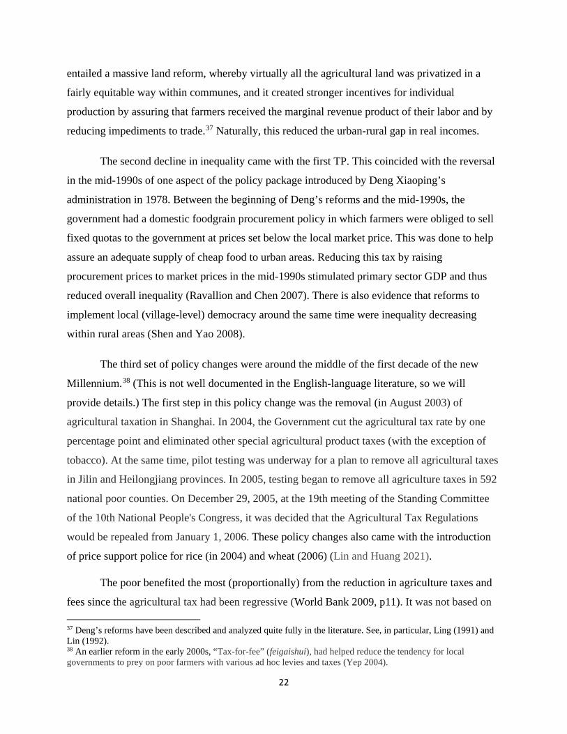
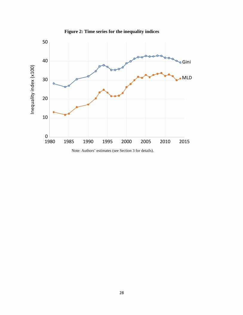
Descriptive results: Applying these methods to the tabulated income distributions
produced by NBS we obtain Figure 2, which shows how the Gini index and MLD have evolved
over time. Tables 1 and 2 provide our estimates by year. Both measures show a strong positive
trend over the period, with rates of increase of 0.48 pp and 0.53 pp per annum for the Gini index
and MLD respectively (using regressions of each index on time, with robust standard errors of
0.09 and 0.10 pp respectively). We also see a marked TP around 2008/09, with a downward
trend since then.
As is well known, unambiguous rankings of distributions in terms of inequality are not
possible if Lorenz curves intersect internally; the ranking will depend on specific attributes of the
inequality index. However, between the low point in China’s Gini index (1984) and the high
point (2008), one finds Lorenz dominance, implying that all inequality measures satisfying the
usual Pigou-Dalton transfer principle will range the distributions the same way (Atkinson 1970).
Lorenz dominance also holds between 2008 and 2014, indicating that the main TP is also robust
to the choice of inequality index.22 While we only provide two specific inequality indices in this
paper, this basic pattern in the data of a longer-term increase in inequality, and a major turning
point after 2008 is robust to the choice of measure.
Notice that there is another “inverted U” TP in the mid-1990s (Figure 2). There are three
periods of declining inequality, namely the early-1980s, the mid-1990s and the mid-2000s
(Figure 2). The first was in 1994. Someone writing this paper around 20 years ago may well have
declared that a Kuznets TP had occurred already. Within a few years, however, the upward
trajectory for overall inequality had been restored (Figure 2). A little over 10 years later a new
TP appeared, in the period 2008-09, with 2008 as the peak in the Gini index. The first TP within
this period was at an urban population share of 30% (for both inequality measures) while the
second was at 44% for the Gini index and 48% for MLD. The decline after the first TP did not
last, but that for the second continues. Over the period as a whole, the three series in Figure 2 are
more like roller coasters than inverted U’s.
The fact that we see more than one TP does not (on its own) rule out the possibility of a
Kuznets process at work. There may well have been an inequality-increasing shocks, side-by-
22 These claims on Lorenz dominance are readily verified using the distributions for China in PovcalNet.

13
side with urbanization, such that a new Kuznets curve emerges after the shock. Section 4 will
provide simulations that isolate the Kuznets effect.
The second TP has attracted much more attention. Indeed (to our knowledge), all those
who refer to China reaching its Kuznets or Lewis turning point refer only to the second TP,
ignoring the first. (It is not uncommon to see graphs of China’s Gini index or its urban-rural
income gap, starting around 2000.) The trend rates of decline after 2008 are of similar (absolute)
magnitude to the prior upwards trends. For the Gini index the trend rate of decrease after 2008 is
almost identical to that before (-0.66 pp per annum after 2008, with a s.e.=0.04 pp, versus a rate
of prior increase of 0.65 pp, with s.e.=0.04). MLD saw somewhat lower rates of decrease after
2008 compared to before (-0.65 pp after versus 0.86 pp). For both inequality indices, the
difference in the coefficients before and after 2008 is statistically significant.23
Two further points are immediate from Figure 3, which plots the Gini indices for urban
and rural areas. First, as noted in the Introduction, the Gini index is higher in rural China than
urban China, though there are signs of inequality convergence between the two sectors.
Recalling the change in NBS surveys in 2013, it is notable that the urban Gini index rose sharply
in 2013, with a mirror-image reversal in rural areas. If the change in 2013 was due to the
aforementioned changes in sampling (Section 3) then one would expect it to persist in the
following year. Instead, we see the Gini index bounce back, largely re-aligned with its pre-2013
trend in the following year (2014). With only two years this cannot be conclusive, but it does not
suggest that the sampling changes in 2013 point to the need for an overall adjustment of the time
series data on inequality.
Second, inequality did not remain constant within each sector, but trended upwards. This
would of course put upward pressure on overall inequality. However, from around 2005, the Gini
indices become close to stationary in both sectors, albeit with fluctuations.
Could it be that the urbanization process has been driving inequality upwards within
either rural or urban areas? This is not easy to assess, given that the urban population share is
highly correlated with time (Figure 1). Controlling for a trend and the lagged value, we find no
23 The differences in the regression coefficients on time are -1.31 and -1.82 with robust standard errors of 0.06 and 0.07 respectively.

14
correlation between the urban population share and the rural Gini index (prob.=0.16), but there is
a strong negative correlation with the urban Gini index (prob.<0.00005).24 So we find some signs
here that the urbanization process was actually inequality decreasing within urban areas.
4. The Kuznets process and MLD
We now take a closer look at MLD, the decomposability properties of which lend itself to
a deeper investigation of whether the pattern in Figure 2 is in fact a Kuznets curve.
MLD in theory: The overall MLD is the sum of within-sector and between-sector values:
MLD = MLD𝑊𝑊 + MLD𝐵𝐵 (1)
where the “within” (MLD𝑊𝑊) and “between” (MLD𝐵𝐵) components are:
MLD𝑊𝑊 = S. MLDU + (1 − S). MLDR (2.1)
MLD𝐵𝐵 = 𝑙𝑙𝑛𝑛(SY�U + (1 − S)Y�R) − (S. 𝑙𝑙𝑛𝑛Y�U + (1 − S). 𝑙𝑙𝑛𝑛Y�R) (2.2)
Here MLD𝑖𝑖 (𝑖𝑖 = U, R) are the MLD measures and Y�𝑖𝑖 (𝑖𝑖 = U, R) are the mean incomes, for urban
and rural areas respectively. Equation (2.2) can be re-written as:
MLD𝐵𝐵 = 𝑙𝑙𝑛𝑛[S.Ψ + (1 − S)] − S. 𝑙𝑙𝑛𝑛Ψ (3)
where Ψ ≡ Y�U/Y�R, the ratio of the urban to the rural mean. Equation (3) shows that the between-
sector MLD depends solely on the urban population share and the ratio of the urban mean to the
rural mean. The Kuznets derivative can be written as:
𝜕𝜕MLD𝜕𝜕S
= 𝜕𝜕MLD𝑊𝑊
𝜕𝜕S+ 𝜕𝜕MLD𝐵𝐵
𝜕𝜕S (4)
where:
𝜕𝜕MLD𝑊𝑊
𝜕𝜕S= MLDU − MLDR (5.1)
𝜕𝜕MLD𝐵𝐵
𝜕𝜕S= Y�U−Y�R
Y�− 𝑙𝑙𝑛𝑛 �Y
�UY�R� = Ψ−1
1+S.(Ψ−1)− 𝑙𝑙𝑛𝑛Ψ (5.2)
24 The regression coefficient on S (x100) is -1.29, with a robust standard error of 0.19. (The other regressors were the lagged urban Gini index and time, which had a regression coefficient of 1.77 (s.e.=0.25).
15
(Recall that, in keeping with the KH, this is a partial derivative holding the distribution constant
within each sector.)
The Kuznets derivative helps us understand when a TP can be expected with
urbanization. In the special case of the Lewis (1954) model, we have MLDU = MLDR = 0, so all
that matters is the between-sector component. Clearly, the between-sector component is a strictly
concave function of the urban population share (𝜕𝜕2MLD𝐵𝐵/𝜕𝜕S2 < 0). So, if there is a Lewis TP,
there can only be one. But is there even one (for 0 ≤ S ≤ 1)? It must be the case that Ψ− 1 ≥
𝑙𝑙𝑛𝑛Ψ for any Ψ > 1.25 Then, on evaluating (5.2) at S = 0, we see that in the Lewis model, and the
Kuznets model with MLDU > MLDR (Assumption (i)), the national MLD must increase in the
initial stages of urbanization (𝜕𝜕MLD/𝜕𝜕S > 0).
At the opposite extreme, consider the point just before the country becomes fully
urbanized. As one approaches the upper limit, S = 1, we have 𝜕𝜕MLD𝐵𝐵/𝜕𝜕S = 1 −Ψ−1 +
𝑙𝑙𝑛𝑛Ψ−1 < 0 (with 0 < Ψ−1 < 1). So, there must be a unique TP for the Lewis model. In other
words, the Lewis TP does not in fact require a narrowing of the urban-rural income gap as the
rural labor surplus is fully absorbed by modern-sector enlargement; the urbanization process
itself will generate the Lewis TP.
For the Kuznets model, however, we cannot sign the Kuznets derivative (𝜕𝜕MLD/𝜕𝜕S) at
S = 1. If MLDU is sufficiently high relative to MLDR then no TP will exist (for 0 ≤ S ≤ 1). The
necessary and sufficient condition for the (interior) Kuznets TP is that MLDU − MLDR < Ψ−1 +
𝑙𝑙𝑛𝑛Ψ − 1 (> 0). That is an empirical issue.
Another factor is the urban-rural gap in mean incomes. Two observations are relevant
here. First, holding distribution within sectors and the urban population share constant, a higher
value of Ψ will be inequality increasing:
𝜕𝜕MLD𝜕𝜕Ψ
= 𝜕𝜕MLD𝐵𝐵
𝜕𝜕Ψ= SY�R �
1Y�− 1
Y�U� > 0 (6)
Second, there is an interaction effect between population urbanization and the urban-rural
income gap, as given by: 25 Note that, since 𝜑𝜑(Ψ) ≡ Ψ− 1 − 𝑙𝑙𝑛𝑛Ψ is strictly convex with its minimum at Ψ = 1, 𝜑𝜑(Ψ) > 0 for all Ψ > 1.

16
𝜕𝜕2MLD𝜕𝜕Ψ𝜕𝜕S
= 1[1+S(Ψ−1)]2
− Ψ−1 (7)
This vanishes in the limit when Ψ = 1, but it also has an interior turning point. For Ψ > 1, it is
readily verified that the sign of the interaction effect is unambiguously positive at S = 0 and
negative at S = 1. In other words, at the beginning of the urbanization process, a larger gap
between urban and rural incomes will make urbanization more inequality increasing, but by the
end of the process the opposite is true—near 100% urbanization, a larger gap makes it more
likely that further urbanization will be inequality decreasing.
MLD in China: Turning to the data for China, Table 2 gives our estimates of MLD and
its urban-rural decomposition as plotted in Figure 4. As for the Gini index, the first TP is in
1994. For MLD the second TP is in the same period as the Gini, though the strict peak is one
year later, in 2009.
Similarly to the Gini index (Figure 3), we see a rise (fall) in the urban (rural) MLD in
2013, but a roughly compensating recovery in 2014. As for the Gini index, we do not see the
kind of persistent effect of the changes in sampling and survey design in 2013 that would warrant
any adjustment to the urban-rural inequality comparisons. However (as noted), other evidence
suggests that the change in sampling alone in 2013 (to include recent migrants) would have
lowered urban inequality.
We see a difference between the first and second TPs in Figure 4. The first stemmed from
TPs in both the between and within components of MLD, and the within component reflected
TPs in both urban and rural inequality. By contrast, the second TP is mainly due to the between-
sector component, which co-moves closely with the overall MLD. If one imagines simply
closing off all changes in the between-sector component—so that changes in overall inequality
were driven solely by the within-sector component—then there would have been no second TP.
We find that two of the three Kuznets assumptions (Section 2) do not hold for MLD in
China. First, we see that there has been a trend increase in the within-sector component of MLD,
though this component has been close to stationary in the new Millennium (Figure 4). When we
decompose the within-sector component we see movements both up and down in the rural MLD,
though in 2014 it was well above its value in 2009—indeed, rural inequality had reached the

17
same level as national inequality, similarly to the beginning of the period (Figure 4). Also, as we
saw for the Gini index, the urbanization process appears to have been inequality decreasing
within urban areas, but had no significant effect on rural inequality.26
Second, consistently with the Gini indices, MLDU < MLDR, so the sign of the Kuznets
derivative at S = 0 is ambiguous, while 𝜕𝜕MLD/𝜕𝜕S < 0 at S = 1. It is unclear whether there will
be a rising segment of the inverted U under the Kuznets process, but the downward segment will
exist. Despite the repeated references in the literature to “China’s Kuznets curve,” it is unclear
whether an urbanization process postulated by Kuznets would yield a Kuznets curve in China.
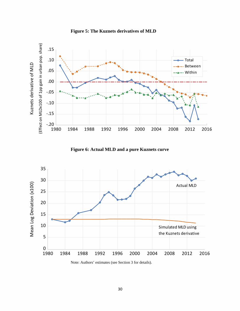
The data can help resolve the matter. Figure 5 shows the Kuznets derivative for China by
year. We find that the Kuznets process would have been inequality decreasing in China in most
years; the exceptions are 1981 and the first half of the 1990s. There are two inverted U’s, with
three TPs: 1983, 1988 and 1999.27
However, what is striking about these estimates of the Kuznets derivatives in Figure 5 is
how small they are, noting that the annualized increase in the urban population share over the
whole period is only 0.011 (about a 1 pp increase per year). Consider, for example, the median
year, 2000. The “within” component of the Kuznets derivative is -0.05 (MLDU=0.17;
MLDR=0.22). This is largely counterbalanced by the “between” component of 0.04 (Y�U =
5.61; Y�R = 2.76; Y� = 3.79). The total Kuznets derivative is only -0.01, or a 1 pp reduction in
the MLD in going from zero urban population share to 100% urbanization. Granted the mean
Kuznets derivative over the entire period is higher, at -0.04, but the point is clear.
To bring the observations in this section together, Figure 6 plots both the actual MLD
(from Figure 4) and a simulation that can be interpreted as the “pure Kuznets curve” for China.
This is obtained by starting from the same value in 1981 but only incrementing the empirical
MLD value for each year by the change in the urban population share multiplied by the Kuznets
derivative. We see that the pure Kuznets process of urbanization would not have generated an
inverted U. The simulated series is essentially flat until the late 1990s, falling thereafter, but with
26 For the urban MLD, the regression coefficient on S (x100) is -0.88 (s.e.=0.17) (with the lagged urban MLD and time as the controls). 27 Using linear interpolation and rounding to the nearest integer.

18
a small gradient. The Kuznets process in China has virtually no power to explain the path of
inequality in China.
Could it be that the urbanization process was in fact driving up the urban-rural income
gap, even though it contributed very little to the rise in overall inequality via the Kuznets process
(recalling that the Kuznets derivative is a partial derivative, holding Y�𝑈𝑈 and Y�𝑅𝑅 constant)? The
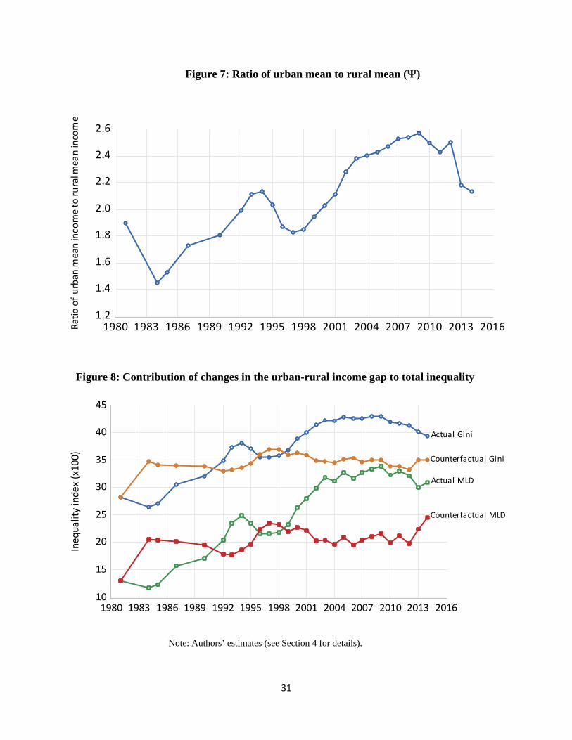
values of Ψ are plotted in Figure 7.28 Again, controlling for the lagged value of Ψ and a time
trend, we find a negative partial correlation between Ψ and S (as %); the regression coefficient is
-0.051 with a standard error of -0.026 (significant at the 6% level). If we use the two-year
moving average of S then there is a small gain in precision (a coefficient of -0.054, s.e.=0.024,
prob.=0.04). So, the data are more suggestive that urbanization has reduced the urban-rural
income gap in China.
5. Alternative explanations for the turning points
This still leaves begging the question as to why we saw the turning points in inequality,
given that it appears to have little to do with the Kuznets Hypothesis. While causal attribution is
difficult (as always), the economic history of China suggests some plausible candidates.
We develop our argument in two steps. First, we demonstrate how important the urban-
rural mean income gap has been to the evolution of overall inequality in China, and we show that
changes in agricultural output per capita were key to the changes in the urban-rural income gap.
Second, we describe the main agrarian policy reforms and when they occurred.
The role of the urban-rural income gap: Comparing Figures 3 or 4 with 7, strong co-
movement is evident; both levels and changes are highly correlated. (In the levels, the correlation
coefficients with Ψ are 0.93 and 0.94 for Gini and MLD respectively; the corresponding
correlations for the first differences are 0.80 and 0.75.) Focusing on the turning points, the first,
in 1994, coincided with a sharp reduction in the ratio of the urban mean to the rural mean (Figure
28 To the extent that income under-reporting is a greater problem in urban areas there will be a bias in the series in Figure 7. The estimates by Piketty et al. (2019 Figure 5) incorporating income tax records and national accounts data show a very similar pattern over time to Figure 7, but with higher ratios of urban to rural, peaking at around the same time but at a level of about 3.7 instead of 2.6.
19
7) for both inequality indices. The next peak in the ratio is in 2009, again coinciding closely with
the TPs in the inequality indices.
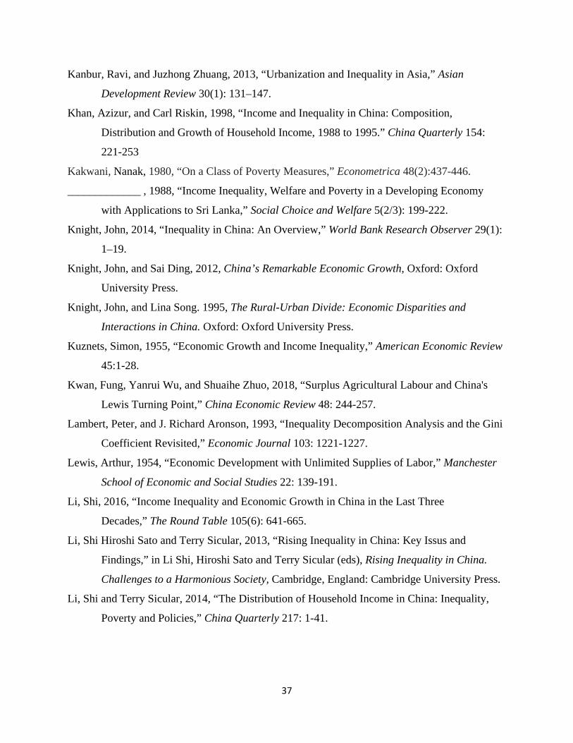
To further quantify the importance of the urban-rural income gap to the TPs, Figure 8
gives the counterfactual series (one for the Gini index and one for MLD) obtained by controlling
for changes in the ratio of the urban mean to the rural mean. For this purpose, a cubic polynomial
in Ψ was used as the regression control function, and the control value was set at the value of Ψ
at the beginning of the series, in 1981.29 We see that without any change in Ψ both TPs would
have vanished (for both inequality indices). The Gini index would have been on a trend decline
since the mid-1990s.30 The MLD would have been a nearly stationary process.
A more flexible representation of the correlation with the distribution of income is found
in Figure 9, which gives the estimated elasticity of the national decile shares to Ψ. These are
estimated using a regression of log decile share on 𝑙𝑙𝑛𝑛Ψ, with controls for both a time trend and
the lagged dependent variable. (Strong serial correlations in the error terms are indicated
otherwise.) We see that the elasticity varies from -0.755 (s.e.=0.116) for the poorest decile to
0.311 (0.114) for the richest, with an elasticity of almost exactly zero at decile 8. The
redistributive impact of the urban-rural income gap is obvious from Figure 9.
In drilling down further, we find a strong link in China between agricultural output and
the gap between urban and rural mean incomes. Regressing the (log) Ψ on (log) primary sector
GDP per capita (GDP1) at constant prices with one-period lags and a time trend, we find that:31
𝑙𝑙𝑛𝑛Ψ = −41.234(18.473)
+ 0.831(0.131)
𝑙𝑙𝑛𝑛Ψ−1 − 1.626(0.299)
𝑙𝑙𝑛𝑛GDP1
+0.858(0.287)
𝑙𝑙𝑛𝑛GDP1−1 + 0.024(0.010)
year + 𝜀𝜀̂ R2=0.896, n=27 (7)
The parameter values are suggestive of a simple difference model:32
29 Polynomials in Ψ were tested up to order 5. For both inequality indices, the cubic gave the best fit using adjusted R2 as the criterion. 30 Post-1995, the trend decline in the Gini index (regressing log Gini on time) is 0.4% per annum (with a standard error of 0.08%). 31 The standard errors (in parentheses) are robust to the presence of both heteroskedasticity and autocorrelation of unknown form (assuming that the autocorrelations fade for more distant observations); see Newey and West (1987). 32 The joint F-test of the parameter restrictions gives F(3,22)=2.76 (prob.=0.07).

20
∆𝑙𝑙𝑛𝑛Ψ = 0.047(0.020)
− 1.013 ∆(0.235)
𝑙𝑙𝑛𝑛GDP1 + 𝜀𝜀̂ R2=0.403, n=27 (8)
In terms of the year-to-year changes we see that Ψ has an elasticity w.r.t. GDP1 of about unity. A
similar elasticity is obtained if one uses agricultural value added per worker at constant prices,
for which the corresponding elasticity is -0.910 (s.e.=0.289).
This is suggestive of the mechanism proposed in Lewis (1954). As noted in the
Introduction, a segment of the literature has declared a “Lewis turning point” in China, having
anticipated this for some time. The theories behind the Kuznets and Lewis TPs are different,
with the latter dependent on the success of the expanding urban economy in absorbing the
(claimed) labor surplus in rural areas. The argument is that once the rural labor surplus is
absorbed, the wage rate of agricultural workers will start to rise. (As noted in Section 5, this is
not in fact required for a Lewis TP.) The data on agricultural output per worker offers some
support for the view that China has recently passed a Lewis turning point. whereby falling
inequality comes in the wake of a large gain in agricultural output per worker.
Given the relatively equitable distribution of agricultural land in China (a legacy of the
Deng’s agrarian reforms), the agricultural labor market is very thin (compared to, say, India).
Nonetheless, the available data on wages for hired farm labor in rural China do suggest a marked
increase around 2004-6, consistent with the idea of a Lewis TP stemming from absorption of the
rural labor surplus (Wang 2010; Cai and Du 2011). Two other sources of data support this view.
The first is agricultural output per worker (which is also in keeping with the formalization of the
Lewis model in Ranis and Fei 1961). Figure 10 gives the series on the growth rate of real
agricultural value added per worker in China.33 We see a marked increase in growth rates from
2004 onwards. The second source is survey data on unskilled, non-agricultural, wages. The
expectation is that these should reflect the change in the opportunity cost of agricultural labor
once the rural labor surplus was absorbed. Cai and Du (2011) and Feng (2013) provide a survey-
based compilation of average wage rates for rural migrant workers in urban areas, which (on
deflating by the CPI) shows a marked increase from the early 2000s. These data are at least
33 The series on agricultural value added per worker is from the World Bank’s World Development Indicators. The series starts in 1991.

21
consistent with the idea that, allowing for a lag, the second inequality TP we see in Figure 2 was
indeed a Lewis TP.
Agrarian policies: There has been a long-standing urban bias in China’s development
policies, with urban areas favored through public subsidies and other forms of public spending
that assured better access in the cities to cheap food, finance, infrastructure, and social policies
including education, health and social protection. The hukou system reinforced this bias, by
restricting migrant access to the services available to registered urban residents. The bias goes
back to development policy making under the Maoist regime in which central planning strived
for rapid industrialization, financed in part by extractive policies in the rural sector.34 The bias
continued into the period of study, though with various reforms (Putterman 1993; Yang 1999).
The urban bias in public spending and the migration restrictions appear to be deeply rooted in
China’s political economy. The urban bias was compounded by a geographic bias in policy
making favoring coastal areas over inland areas.
The main enforcement mechanisms for urban bias have involved various agrarian
policies, and reforms to those policies appear to have been a powerful instrument against
inequality. In what follows we will argue that the history of China’s agrarian policies can help
understand the turning points we have seen in the urban-rural income gap. A key aspect is how
much agriculture was (implicitly or explicitly) taxed to support industrial development. Over
time we have seen a switch from taxing agriculture this way to more neutral and even
agricultural subsidies.35 This did not (of course) happen continuously, but in discrete jumps. We
will argue that these coincided fairly closely with the turning points in inequality.
All three periods of declining inequality in China since 1980 coincided with significant
agrarian reforms. The first was the set of reforms introduced under Deng Xiaoping, notably the
Household Responsibility System, which abandoned collective agriculture to return to peasant
family farming. It is not widely appreciated that the market-based reform agenda that put China
on its impressive trajectory over the last 40 years started in agriculture.36 The first set of reforms
34 For further discussion of this aspect of the history of China’s development policies see Ravallion (2021a) and references therein 35 For a recent review of the history of agricultural policy see Lin and Huang (2021). 36 This observation about the sequencing of reforms is arguably one of the key lessons from China’s success for other developing countries (Ravallion 2009, with reference to lessons for Sub-Saharan Africa).
22
entailed a massive land reform, whereby virtually all the agricultural land was privatized in a
fairly equitable way within communes, and it created stronger incentives for individual
production by assuring that farmers received the marginal revenue product of their labor and by
reducing impediments to trade.37 Naturally, this reduced the urban-rural gap in real incomes.
The second decline in inequality came with the first TP. This coincided with the reversal
in the mid-1990s of one aspect of the policy package introduced by Deng Xiaoping’s
administration in 1978. Between the beginning of Deng’s reforms and the mid-1990s, the
government had a domestic foodgrain procurement policy in which farmers were obliged to sell
fixed quotas to the government at prices set below the local market price. This was done to help
assure an adequate supply of cheap food to urban areas. Reducing this tax by raising
procurement prices to market prices in the mid-1990s stimulated primary sector GDP and thus
reduced overall inequality (Ravallion and Chen 2007). There is also evidence that reforms to
implement local (village-level) democracy around the same time were inequality decreasing
within rural areas (Shen and Yao 2008).
The third set of policy changes were around the middle of the first decade of the new
Millennium.38 (This is not well documented in the English-language literature, so we will
provide details.) The first step in this policy change was the removal (in August 2003) of
agricultural taxation in Shanghai. In 2004, the Government cut the agricultural tax rate by one
percentage point and eliminated other special agricultural product taxes (with the exception of
tobacco). At the same time, pilot testing was underway for a plan to remove all agricultural taxes
in Jilin and Heilongjiang provinces. In 2005, testing began to remove all agriculture taxes in 592
national poor counties. On December 29, 2005, at the 19th meeting of the Standing Committee
of the 10th National People's Congress, it was decided that the Agricultural Tax Regulations
would be repealed from January 1, 2006. These policy changes also came with the introduction
of price support police for rice (in 2004) and wheat (2006) (Lin and Huang 2021).
The poor benefited the most (proportionally) from the reduction in agriculture taxes and
fees since the agricultural tax had been regressive (World Bank 2009, p11). It was not based on 37 Deng’s reforms have been described and analyzed quite fully in the literature. See, in particular, Ling (1991) and Lin (1992). 38 An earlier reform in the early 2000s, “Tax-for-fee” (feigaishui), had helped reduce the tendency for local governments to prey on poor farmers with various ad hoc levies and taxes (Yep 2004).

23
farmer’s net income (or net agriculture income), but rather it was typically based on the size of
land that the farmer contracted. As noted, Deng’s reforms at the time of de-collectivization
assured relatively equitable land allocation. Thus, poor farmers ended up paying a high tax, and
their tax rate (agricultural tax as a share of total net income) could be higher than average, since
poor farmers have less off-farm income. Hence removal of the agriculture tax has a significant
impact on the rural poor. The average agricultural tax cut was about 120 Yuan per capita in
2006, which accounts for 17% of the net income of the poorest 6.1%. The average agricultural
tax rate was only about 3.3% for the rural sector as a whole.39
New policy reforms relevant to the urban-rural component of overall inequality in China
will no doubt emerge over the coming years. The gap in living standards between urban and rural
areas reflects in part a long-standing inequality in social policies (health, education and social
protection) (Knight and Song 1995). The large urban-rural gap in education attainments is of
special concern (Rozelle and Hell 2020). Expanding the coverage of social policies to include
rural areas will clearly reduce urban-rural inequality and (hence) overall inequality in China.40
Further progress toward eliminating the hukou registration system would help in reducing overall
inequality.
6. Conclusions
There has been a tendency to declare a “Kuznets curve” whenever one sees an inverted U
in how some social, economic, political or environmental variable evolves with economic
development. Yet the turning point in the inverted U may have little or nothing to do with the
process of economic development through modern-sector enlargement postulated in the classic
models of Kuznets and Lewis. And the implications (including for policy) may depend on why
we see such a turning point.
The paper has provided new series of inequality measures back to 1981 and used these to
assess whether the claimed “Kuznets curve” for China has anything to do with Kuznets. We
confirm that our new measures look like a “Kuznets curve,” at least since the late 1990s.
39 Authors’ calculations based on the Tables 3.7 and 3.8 in NBS (2007). 40 For example, China’s Dibao program (aiming to provide a floor to incomes using cash and in-kind benefits) started in urban areas, but a version has been created for rural areas.
24
However, our analysis indicates that the country’s turning points for inequality have rather little
to do with the Kuznets Hypothesis as formalized in development economics. We have shown
that the within-sector neutral growth process, as postulated in the Kuznets Hypothesis, would not
have generated the path for inequality measures seen in China. Key assumptions of that model
simply do not hold. Nor do the data for China support the view that the urbanization process has
been driving up urban-rural disparities in mean incomes, or inequalities within either urban or
rural areas; if anything it is the opposite.
The turning points for inequality have clearly stemmed from date-specific reversals in the
longer-term pattern of divergence between urban and rural mean incomes. Indeed, once we
control for the ratio of the urban mean to the rural mean we find no sign of a trend increase (or
decrease) in income inequality in China since the mid-1990s. The counterfactual Gini index
would have seen a trend decline. Causal attribution is difficult of course, but we have also
pointed to specific policy changes that helped the rural sector, and coincided with all three
periods of declining inequality in China’s economic history since 1980, including the two
(known) inverted-U turning points.
Just as China’s first turning point for inequality was short lived, we cannot be complacent
about the latest turning point, which has received so much attention. These reversals in the
direction of change in overall inequality are not the realizations of some more-or-less inevitable,
theoretically grounded, process in economic development through urbanizing structural
transformation. In large part, for China, they appear to reflect policies. Just as we saw in the first
turning point, unless there is a continuing commitment to redistributive effort—which (as in
most developing countries) includes the prioritization given to agriculture and rural
development—China could well return to its upward trajectory for overall inequality.

25
Table 1: Summary statistics and our estimates of the annual Gini
(1) (2) (3) (4) (5) (6) (7) Mean income ($/day/person; 2011 prices) Gini index (x100) Urban pop.
share (%) National Rural Urban National Rural Urban 1981 1.18 1.00 1.89 28.18 24.73 18.46 20.13 1984 1.64 1.49 2.16 26.40 26.69 17.79 22.22 1985 1.72 1.53 2.35 27.04 27.12 17.05 22.86 1987 1.86 1.58 2.73 30.51 29.45 20.20 24.26 1990 1.94 1.60 2.90 32.00 29.87 23.42 26.45 1992 2.19 1.71 3.41 34.81 32.03 24.17 28.20 1993 2.34 1.77 3.73 37.27 33.71 27.18 29.11 1994 2.54 1.90 4.05 38.00 33.84 29.22 30.04 1995 2.75 2.09 4.25 37.02 33.98 28.27 30.95 1996 3.01 2.36 4.41 35.43 32.98 28.52 31.91 1997 3.18 2.50 4.56 35.42 33.12 29.35 32.89 1998 3.36 2.61 4.82 35.87 33.07 29.94 33.87 1999 3.6 2.71 5.27 36.84 33.91 29.71 34.86 2000 3.79 2.76 5.61 38.94 35.70 31.87 35.89 2001 4.07 2.88 6.09 39.97 36.49 32.32 37.09 2002 4.52 3.03 6.90 41.35 37.03 32.65 38.43 2003 4.89 3.16 7.53 42.27 38.04 32.51 39.77 2004 5.32 3.37 8.10 42.12 36.84 33.32 41.14 2005 5.88 3.66 8.88 42.83 37.68 34.01 42.52 2006 6.53 3.97 9.81 42.54 37.33 33.66 43.87 2007 7.36 4.35 11.00 42.61 37.38 33.26 45.20 2008 8.06 4.69 11.93 42.96 37.70 34.02 46.54 2009 8.93 5.10 13.10 42.91 38.41 33.52 47.88 2010 9.82 5.65 14.12 41.87 37.79 33.01 49.23 2011 10.85 6.30 15.30 41.67 39.01 32.91 50.57 2012 11.93 6.70 16.78 41.22 38.66 31.64 51.89 2013 13.15 8.07 17.63 40.16 36.51 34.01 53.17 2014 14.26 8.82 18.81 39.38 37.74 32.86 54.41 Note: Authors’ calculations based on distributions of household per capita income produced by China’s National Bureau of Statistics. (See text for details.)

26
Table 2: MLD and its rural-urban decomposition
(1) (2) (3) (4) (5) Rural Urban Within Between Total MLD
1981 10.20 5.90 9.33 3.73 13.06 1984 11.81 5.36 10.38 1.28 11.65 1985 12.28 4.80 10.57 1.72 12.28 1987 14.56 6.94 12.71 2.99 15.70 1990 14.81 9.35 13.36 3.70 17.07 1992 17.27 9.76 15.15 5.24 20.39 1993 19.32 12.17 17.24 6.27 23.51 1994 20.13 14.15 18.34 6.55 24.89 1995 19.63 13.21 17.64 5.79 23.44 1996 18.72 13.40 17.02 4.50 21.52 1997 18.89 14.24 17.36 4.22 21.58 1998 18.57 15.04 17.37 4.45 21.82 1999 19.65 14.69 17.92 5.29 23.21 2000 22.18 17.02 20.33 6.05 26.38 2001 23.36 17.49 21.18 6.81 27.99 2002 23.89 17.98 21.62 8.35 29.96 2003 25.46 17.81 22.42 9.31 31.73 2004 23.78 18.71 21.69 9.50 31.19 2005 25.62 19.47 23.01 9.74 32.75 2006 24.52 19.05 21.58 10.10 31.68 2007 24.96 18.62 22.10 10.61 32.71 2008 25.53 19.55 22.75 10.66 33.41 2009 26.66 18.94 22.97 10.86 33.83 2010 25.35 18.70 22.08 10.18 32.26 2011 28.73 18.28 23.44 9.53 32.97 2012 27.73 16.74 22.02 10.05 32.07 2013 25.59 20.13 22.68 7.29 29.97 2014 30.43 18.72 24.06 6.80 30.86 Note: MLDx100. Authors’ calculations based on distributions of household per capita income produced by China’s National Bureau of Statistics. (See text for details.)

27
Figure 1: Urbanization in China
.0
.1
.2
.3
.4
.5
.6
1980 1984 1988 1992 1996 2000 2004 2008 2012 2016
Urb
an p
opul
atio
n sh
are
Slope=0.0110 (s.e.=0.0003)
Note: Urban population shares implicit in estimates of mean incomes for urban, rural and national from China’s National Bureau of Statistics.
28
Figure 2: Time series for the inequality indices
0
10
20
30
40
50
1980 1985 1990 1995 2000 2005 2010 2015
Gini
MLD
Ineq
ualit
y in
dex
(x10
0)
Note: Authors’ estimates (see Section 3 for details).

29
Figure 3: Gini indices
10
15
20
25
30
35
40
45
1980 1983 1986 1989 1992 1995 1998 2001 2004 2007 2010 2013 2016
NationalRuralUrban
Gin
i ind
ex o
f inc
ome
ineq
ualit
y (x
100)
Figure 4: MLD and its decomposition
0
5
10
15
20
25
30
35
1980 1984 1988 1992 1996 2000 2004 2008 2012 2016
TotalRuralUrbanWithi nBetween
MLD
and
its c
ompo
nent
s (x1
00)
Note: Authors’ estimates (see Section 3 for details).
30
Figure 5: The Kuznets derivatives of MLD
-.20
-.15
-.10
-.05
.00
.05
.10
.15
1980 1984 1988 1992 1996 2000 2004 2008 2012 2016
TotalBetweenWithin
Kuzn
ets
deriv
ativ
e of
MLD
(Eff
ect o
n M
LDx1
00 o
f 1pp
gai
n in
urb
an p
op. s
hare
)
Figure 6: Actual MLD and a pure Kuznets curve
0
5
10
15
20
25
30
35
1980 1984 1988 1992 1996 2000 2004 2008 2012 2016
Mea
n Lo
g De
viat
ion
(x10
0) Actual MLD
Simulated MLD using the Kuznets derivative
Note: Authors’ estimates (see Section 3 for details).
31
Figure 7: Ratio of urban mean to rural mean (𝚿𝚿)
1.2
1.4
1.6
1.8
2.0
2.2
2.4
2.6
1980 1983 1986 1989 1992 1995 1998 2001 2004 2007 2010 2013 2016Ratio
of u
rban
mea
n in
com
e to
rura
l mea
n in
com
e
Figure 8: Contribution of changes in the urban-rural income gap to total inequality
10
15
20
25
30
35
40
45
1980 1983 1986 1989 1992 1995 1998 2001 2004 2007 2010 2013 2016
Actual Gini
Ineq
ualit
y in
dex
(x10
0) Counterfactual Gini
Actual MLD
Counterfactual MLD
Note: Authors’ estimates (see Section 4 for details).

32
Figure 9: Elasticities of decile shares to the urban-rural income gap
-1.0
-0.8
-0.6
-0.4
-0.2
0.0
0.2
0.4
0.6
1 2 3 4 5 6 7 8 9 10
Elas
ticity
of d
ecile
sha
re
w.r.
t urb
an-r
ural
inco
me
g ap
Decile (poorest) (richest)
Note: Based on regressions of log decile shares on the log of the ratio of the urban mean to the rural mean, including the lagged dependent variable and a time trend. Bands indicate +/- two (robust) standard errors. N=27.

33
Figure 10: Agricultural value added per worker
0
2
4
6
8
10
12
1992 1994 1996 1998 2000 2002 2004 2006 2008 2010 2012 2014 2016
Gro
wth
rate
of a
gric
ultu
ral v
alue
add
ed p
er w
orke
r
(con
stan
t 201
0 pr
ices
; % p
er a
nnum
)
Note: 2010 prices. Includes forestry and fishing, Source: World Bank’s World Development Indicators, combining output data from the national accounts with employment data from the ILO.

34
References Adelman, Irma, and Sherman Robinson, 1988, ‘‘Income Distribution and Development,’’ in
Handbook of Development Economics Vol. 1, H. Chenery and T. N. Srinivasan (eds),
Amsterdam: North-Holland.
Ahluwalia, Montek, 1976, “Inequality, Poverty, and Development,” Journal of Development
Economics 3: 307-342.
Anand, Sudhir, and Ravi Kanbur, 1993a, “The Kuznets Process and the Inequality-Development
Relationship,” Journal of Development Economics 40:25-52.
____________, and __________, 1993b, “Inequality and Development: A Critique,” Journal of
Development Economics 41: 19-43.
Atkinson, Anthony B., 1970, “On the Measurement of Inequality,” Journal of Economic Theory
2: 244-263.
Barro, Robert, 2000, “Inequality and Growth in a Panel of Countries.” Journal of Economic
Growth 5: 5–32.
Benjamin, Dwayne, Loren Brandt, and John Giles, 2005, “The Evolution of Income Inequality in
Rural China.” Economic Development and Cultural Change 53(4): 769–824.
Bourguignon, François, 1979, “Decomposable Income Inequality Measures,” Econometrica, 47:
901-920.
Bruno, Michael, Martin Ravallion and Lyn Squire, 1998, “Equity and Growth in Developing
Countries: Old and New Perspectives on the Policy Issues,” in Vito Tanzi and Ke-young
Chu (eds) Income Distribution and High-Quality Growth, Cambridge: MIT Press.
Cai, Fang, 2021, “The Income Distribution Kuznets Turning Point,” in Fang Cai, Understanding
China's Economy: The Turning Point and Transformational Path of a Big Country, pp.
195-206, Springer.
Cai, Fang, and Yang Du, 2011, “Wage Increases, Wage Convergence, and the Lewis Turning
Point in China,” China Economic Review 22(4): 601-610.
Cai, Fang, and Meiyan Wang, 2010, “Growth and Structural Changes in Employment in
Transition China,” Journal of Comparative Economics 38: 71-81.

35
Chen, Shaohua, and Martin Ravallion, 2008, “China is Poorer than we Thought, but no Less
Successful in the Fight against Poverty,” Policy Research Working Paper No. 4621,
World Bank, Washington DC.
____________, and ______________, 2010, “The Developing World is Poorer than we
Thought, but no Less Successful in the Fight against Poverty,” Quarterly Journal of
Economics, 125(4): 1577-1625.
____________, and ______________, 2021, “Reconciling the Conflicting Narratives on Poverty
in China,” Journal of Development Economics 153 (November): in progress.
Cheng, Wenli, and Yongzheng Wu, 2017, “Understanding the Kuznets Process—An Empirical
Investigation of Income Inequality in China: 1978–2011,” Social Indicators Research
134: 631-650.
Cowell, Frank, and Emmanuel Flachaire, 2018, “Inequality Measures and the Rich: Why
Inequality Increased more than we Thought,” mimeo, London School of Economics.
Datt, Gaurav, and Martin Ravallion, 1992, “Growth and Redistribution Components of
Changes in Poverty Measures: A Decomposition with Applications to Brazil and India in
the 1980s,” Journal of Development Economics 38: 275-295.
Deininger, Klaus, and Lyn Squire, 1998, “New Ways of Looking at Old Issues: Inequality and
Growth,” Journal of Development Economics 57(2): 259-87.
Du, Yang, and Wang Meiyan, 2010, “Discussions on Potential Bias and Implications of Lewis
Turning Point,” China Economic Journal 3(2): 121–136.
Duesenberry, James S., 1949, Income, Saving and the Theory of Consumer Behavior,
Cambridge, Mass.: Harvard University Press.
Fei, John C.H., and Gustav Ranis, 1964, Development of the Labor Surplus Economy: Theory
and Policy, Homewood, Ill: Irwin.
Feng, Lu, 2013, “Wage Levels of Rural Migrant Workers in China during 1979-2010: Estimates
and Trends,” China Economist 8(1): 4-22.
Ferreira Francisco, Shohua Chen, A. Dabalen, Y. Dikhanov, N. Hamadeh, D. Joliffe, A. Narayan
E. Prydz, A. Revenga, P. Sangraula, U. Serajuddin, and N. Yoshida, 2016, “A Global
Count of the Extreme Poor in 2012: Data Issues, Methodology and Initial Results,”
Journal of economic inequality 14: 141-172.

36
Fields, Gary S., 1979. “A Welfare Economic Approach to Growth and Distribution in the Dual
Economy,” Quarterly Journal of Economics 93: 325–353.
____________, 2001, Distribution and Development, A New Look at the Developing World.
New York: Russel Sage Foundation and Cambridge, Massachusetts: MIT Press.
Financial Times, 2015, “China at the Lewis Turning Point,” FT World, May 4.
Gallup, John Luke, 2012, “Is There a Kuznets Curve?” Portland State University.
Garnaut, Ross, and Yiping Huang. 2006. “Continued Rapid Growth and The turning Point in
China’s Economic Development,” in Ross Garnaut and Ligang Song (eds), The Turning
Point in China’s Economic Development, Canberra: Asia Pacific Press, Australian
National University.
Giles, John and Ren Mu, 2018, “Village Political Economy, Land Tenure Insecurity, and the
Rural to Urban Migration Decision: Evidence from China,” American Journal of
Agricultural Economics 100(2): 521-544.
Gradín, Carlos, Murray Leibbrandt, and Finn Tarp, 2021, “Setting the Scene” in Carlos Gradín,
Murray Leibbrandt, and Finn Tarp (eds) Inequality in the Developing World. Oxford:
Oxford University Press.
Huang, Yiping and Fang Cai (eds), 2014, Debating the Lewis Turning Point in China, London:
Routledge.
Islam, Nazrul, and Kazuhiko Yokota, 2008, “Lewis Growth Model and China’s
Industrialization,” Asian Economic Journal 22(4): 359–396.
Jalil, Abdul, 2012, “Modeling Income Inequality and Openness in the Framework of Kuznets
Curve: New Evidence from China,” Economic Modelling 29(2): 309-315.
Jha, Sailesh, 1996, “The Kuznets Curve: A Reassessment,” World Development 24(4): 773-780.
Jorgenson, Dale, 1967, “Surplus Labour and the Development of a Dual Economy,” Oxford
Economic Papers 19(3): 288-312.
Kanbur, Ravi, 2019, “Structural Transformation and Income Distribution: Kuznets and Beyond,”
in Célestin Monga, Justin Yifu Lin (eds), The Oxford Handbook of Structural
Transformation, Oxford: Oxford University Press.
Kanbur, Ravi, Yue Wang, and Xiaobo Zhang, 2021, “The Great Chinese Inequality
Turnaround,” Journal of Comparative Economics 49: 467-482.
37
Kanbur, Ravi, and Juzhong Zhuang, 2013, “Urbanization and Inequality in Asia,” Asian
Development Review 30(1): 131–147.
Khan, Azizur, and Carl Riskin, 1998, “Income and Inequality in China: Composition,
Distribution and Growth of Household Income, 1988 to 1995.” China Quarterly 154:
221-253
Kakwani, Nanak, 1980, “On a Class of Poverty Measures,” Econometrica 48(2):437-446.
_____________ , 1988, “Income Inequality, Welfare and Poverty in a Developing Economy
with Applications to Sri Lanka,” Social Choice and Welfare 5(2/3): 199-222.
Knight, John, 2014, “Inequality in China: An Overview,” World Bank Research Observer 29(1):
1–19.
Knight, John, and Sai Ding, 2012, China’s Remarkable Economic Growth, Oxford: Oxford
University Press.
Knight, John, and Lina Song. 1995, The Rural-Urban Divide: Economic Disparities and
Interactions in China. Oxford: Oxford University Press.
Kuznets, Simon, 1955, “Economic Growth and Income Inequality,” American Economic Review
45:1-28.
Kwan, Fung, Yanrui Wu, and Shuaihe Zhuo, 2018, “Surplus Agricultural Labour and China's
Lewis Turning Point,” China Economic Review 48: 244-257.
Lambert, Peter, and J. Richard Aronson, 1993, “Inequality Decomposition Analysis and the Gini
Coefficient Revisited,” Economic Journal 103: 1221-1227.
Lewis, Arthur, 1954, “Economic Development with Unlimited Supplies of Labor,” Manchester
School of Economic and Social Studies 22: 139-191.
Li, Shi, 2016, “Income Inequality and Economic Growth in China in the Last Three
Decades,” The Round Table 105(6): 641-665.
Li, Shi Hiroshi Sato and Terry Sicular, 2013, “Rising Inequality in China: Key Issus and
Findings,” in Li Shi, Hiroshi Sato and Terry Sicular (eds), Rising Inequality in China.
Challenges to a Harmonious Society, Cambridge, England: Cambridge University Press.
Li, Shi and Terry Sicular, 2014, “The Distribution of Household Income in China: Inequality,
Poverty and Policies,” China Quarterly 217: 1-41.

38
Li, Shi Terry Sicular, and Finn Tarp, 2021, “China: Structural Change, Transition, Rent-Seeking
and Corruption, and Government Policy,” in Carlos Gradín, Murray Leibbrandt, and Finn
Tarp (eds) Inequality in the Developing World. Oxford: Oxford University Press.
Lin, Justin Yifu, 1992, “Rural Reforms and Agricultural Growth in China.” American Economic
Review 82: 34–51.
_____________, 2009, Economic Development and Transition. Thought, Strategy and Viability.
Cambridge: Cambridge University Press.
Lin, Wensheng, and Jikun Huang, 2021, “Impacts of Agricultural Incentive Policies on Land
Rental Prices: New Evidence from China,” Food Policy 104: 1-11.
Ling, Zhu, 1991, Rural Reform and Peasant Income in China: The Impact of China's Post-Mao
Rural Reforms in Selected Regions. London and Basingstoke: Macmillan.
Lipton, Michael, and Martin Ravallion, 1995, “Poverty and Policy,” in Jere Behrman and T.N.
Srinivasan (eds) Handbook of Development Economics, Volume 3, Amsterdam: North-
Holland.
Milanovic, Branko, 2000, “Determinants of Cross-Country Income Inequality: An
‘Augmented’ Kuznets Hypothesis,” in Vojmir Franičević Milica Uvalić (eds) Equality,
Participation, Transition, London: Palgrave Macmillan.
_______________, 2016a, “Introducing Kuznets Waves: How Income Inequality Waxes and
Wanes over the Very Long Run,” VOX-EU Post, 24 February.
_______________, 2016b, Global Inequality. A New Approach for the Age of Globalization,
Cambridge Mass.: Harvard University Press.
National Bureau of Statistics (NBS), 2007, China Rural Household Survey Yearbook 2007.
Beijing: National Bureau of Statistics.
Newey, Whitney and Kenneth West, 1987, “A Simple Positive Semi-Definite, Heteroskedasticity
and Autocorrelation Consistent Covariance Matrix,” Econometrica 55: 703–708.
Piketty, Thomas, 2014, Capital in the Twenty-First Century, Cambridge, Mass.: Harvard
University Press.
Piketty, Thomas, Li Yang, and Gabriel Zucman, 2019, “Capital Accumulation, Private Property,
and Rising Inequality in China,1978–2015,” American Economic Review 109(7): 2469–
2496
39
Putterman, Louis, 1993, Continuity and Change in China's Rural Development: Collective and
Reform Eras in Perspective. New York: Oxford University Press.
Ram, Rati, 1995, ‘‘Economic Development and Inequality: An Overlooked Regression
Constraint,’’ Economic Development and Cultural Change 43: 425–34.
Ranis, Gustav, and John C. H. Fei, 1961, “A Theory of Economic Development,” American
Economic Review 51(4): 533-565.
Ravallion, Martin, 1997, “On Rati Ram's Test of the Kuznets Hypothesis,” Economic
Development and Cultural Change 46(1): 187-190.
_______________, 2009, “Are there Lessons for Africa from China’s Success Against Poverty?”
World Development, 37(2): 303-313.
_______________, 2010, “The Developing World’s Bulging (but Vulnerable) Middle Class,”
World Development 38(4): 445-454.
_______________, 2021a, “Poverty in China since 1950: A Counterfactual Perspective,” NBER
Working Paper 28370.
_______________, 2021b, “Missing Top Income Recipients,” NBER Working Paper 28890.
Ravallion, Martin, and Shaohua Chen, 2007, “China’s (Uneven) Progress Against Poverty.”
Journal of Development Economics 82(1): 1-42.
Robinson, Sherman, 1976, “A Note on the U-Hypothesis Relating Income Inequality and
Economic Development,” American Economic Review 66:437-440.
Rosenzweig, Mark, 1988, “Labor Markets in Developing Countries,” in H. Chenery and T.N.
Srinivasan (eds) Handbook of Development Economics, Vol. 1. Amsterdam: North
Holland.
Rozelle, Scott, and Natalie Hell, 2020, Invisible China, How the Urban-Rural Divide Threatens
China’s Rise. Chicago: University of Chicago Press.
Schultz, Theodore W., 1964, Transforming Traditional Agriculture. New Haven: Yale University
Press.
Shen, Yan, and Yang Yao, 2008, “Does Grassroots Democracy Reduce Income Inequality in
China?” Journal of Public Economics 92: 2182–2198.
Sicular, Terry, Ximing Yue, Björn Gustafsson, and Li, Shi, 2006, “The Urban Rural Income Gap
and Inequality in China,” WIDER Research Paper, No. 2006/135, WIDER, Helsinki.
Theil, Henri, 1967, Economics and Information Theory, Amsterdam: North-Holland.

40
Timmer Peter, 2002, “Agriculture and Economic Development,” Handbook of Agricultural
Economics 2(A): 1487-1546.
Wan, Guanghua, Ting Wu, and Yan Zhang, 2018, “The Decline of Income Inequality in China:
Assessments and Explanations,” Asian Economic Papers 17(3): 115-141.
Wang, Chen, Guanghua Wan, and Dan Yang, 2014, “Income Inequality in the People’s Republic
of China: Trends, Determinants, and Proposed Remedies.” Journal of Economic Surveys
28(4): 686–708.
Wang, Meiyan, 2010, “The Rise of Labor Cost and the Fall of Labor Input: Has China Reached
Lewis Turning Point?” China Economic Journal 3(2): 139-155.
Wang, Xiaolu, 2006, “Income Inequality in China and its Influencing Factors,” WIDER
Research Paper, No. 2006/126.
World Bank, 2009, From Poor Areas to Poor People: China’s Evolving Poverty Reduction
Agenda. An Assessment of Poverty and Inequality in China, Washington DC: World
Bank.
Yang, Dennis T., 1999, “Urban-Based Policies and Rising Income Inequality in China,”
American Economic Review, Papers and Proceedings 89(2): 306-310.
Yang Jun, and Zongyi Zhang, 2003, “Income Distribution in China's Economic Development
and Kuznets U hypothesis,”《数量经济技术经济研究》(Journal of Quantitative and
Technical Economics) No. 2.
Yep, Ray, 2004, “Can ‘Tax-for-Fee’ Reform Reduce Rural Tension in China? The Process,
Progress and Limitations,” China Quarterly 177 (Mar.): 42-70.
Young, Jason, 2013, China's Hukou System: Markets, Migrants and Institutional Change.
Basingstoke: Palgrave Macmillan.
Zhang, Xiaobo, J Yang and S Wang, 2011, “China has Reached the Lewis Turning Point,” China
Economic Review 22(4): 542-554.


