1
Is the Millennium Development Goal of Income Poverty Still Achievable? Role of Institutions, Finance and Openness
Katsushi S. Imai*†
Economics, School of Social Sciences, University of Manchester, UK
Raghav Gaiha
Faculty of Management Studies, University of Delhi, India
Ganesh Thapa
International Fund for Agricultural Development, Rome, Italy
&
Samuel Annim
Economics, School of Social Sciences, University of Manchester, UK
Abstract
Drawing upon the new World Bank poverty data, the present analysis examines the feasibility of achieving the Millennium Development Goal of income poverty (MDG1) where the inter-relationships are taken account of between finance, institutions, trade liberalisation and growth, and poverty. Our econometric results suggest a slowing down of poverty reduction in more recent years after 2000 in the parsimonious specification. Also confirmed are (i) the roles of better institutions in income growth, poverty reduction, trade openness, and financial development, (ii) the role of financial development in economic growth, (iii) the positive effect of capital liberalisation on financial development. Simulations for different regions show that MDG1 will be achieved in most regions if historical growth rate is maintained in 2006-2015, while the improvement in institutional quality is crucial for halving poverty for Sub Saharan Africa.
*Contact Address Katsushi S. Imai (Dr) Economics, School of Social Sciences, University of Manchester, Arthur Lewis Building, Oxford Road, Manchester M13 9PL, UK; Telephone: +44-(0)161-275-4827, Fax: +44-(0)161-275-4812 Email: [email protected].
2
Is the Millennium Development Goal of Income Poverty Still Achievable? Role of Institutions, Finance and Openness
1. Introduction
At the Millennium Summit in September, 2000, world leaders committed the global
community to halve by 2015 the proportions of poor and hungry. They also pledged in the
United Nations Millennium Declaration to achieve other Millennium Development Goals
(MDGs) encompassing education, gender equality, and women’s empowerment, health and
communicable diseases such as HIV/AIDS and malaria, and environmental sustainability. In
brief, these goals aim for a broader and more inclusive process of human development.
The MDGs are ambitious, as they represent clear and direct challenges both to individual
countries and to the global community. Achievement of these goals in Asia and the Pacific
Region –especially in South Asia- is of considerable importance because of the pervasiveness
of different forms of deprivation.
While the progress achieved in meeting the MDGs-especially ‘MDG1’ of reducing by half
the proportion of people living on less than a dollar a day- is laudable, new estimates of
poverty in the developing world produced by Chen and Ravallion (2008) raise concerns as
the incidence of poverty is considerably higher than in their previous estimate. These
estimates are based on the new purchasing power parity estimates for 2005. A review of
progress achieved towards MDG1 is thus necessary. This is the motivation for the present
study. The main objective of this study is to evaluate the feasibility of MDG1 for income
poverty based on the new estimates of poverty.
Chen and Ravallion (2008) justify their new estimates on the following grounds. First, they
used the 2005 ICP. This is a large advance on the 1993 estimates as the number of countries
included is much larger (China, for example, participated in the 2005 ICP for the first time)
3
and the quality of price data is considerably better. Secondly, an updated poverty line is used
and its robustness is confirmed. The new poverty line of $1.25 per day in 2005, which was
first updated by Ravallion et al. (2008), is deliberately lower than the 2005 value in US
dollars of the previous poverty line. The new line is the mean of the national poverty lines for
the poorest 15 countries in terms of consumption per capita. New poverty estimates
correspond to a range of poverty lines spanning $1.00 to $2.50 per day in 2005 prices.
The coverage of household surveys is also much larger in their new study, altogether 675
surveys, spanning 1979-2006 and 116 countries. The incidence of global poverty is higher
than past estimates, mainly because the 2005 ICP data suggest that past PPPs had implicitly
underestimated the cost of living in most developing countries.
To summarise the claims made by Chen and Ravallion (2008), (i) 1.4 billion people are
found to live below the $1.25 line; (ii) About 26 % of the developing world’s population in
2005 is poor versus 17 % using the old line at 1993 PPP-an extra 400 million people living in
poverty; (iii) Over the period 1981-2005, the percentage of poor almost halved, falling from
52 % to 26 % (expressed as a proportion of the population of the world, the decline is from
42 % to 22%); (iv) The number of poor fell by about 500 million, from 1.9 billion to 1.4
billion over this period; (v) The trend rate of decline was 1 % point per year, and it is slightly
higher than the trend decline obtained from the 1993 PPPs (-0.83 % per year); (vi) The 1 %
per year rate of decline in poverty also holds in the period since 1990; (vii) There is,
however, much less progress in getting above the $2 per day line; (viii) The poverty rate fell
from 70 % in 1981 to 48 % in 2005; and (ix) The trend reduction is 0.8 % per year, but
excluding China, the trend reduction is only 0.3 % point per year. Chen and Ravallion (2008,
p.25) offer an optimistic assessment: ‘While the new data suggest that the developing world
is poorer than we thought, it has been no less successful in reducing the incidence of absolute
poverty since the early 1980s. …….The developing world as a whole is clearly on still on
4
track to attaining the first Millennium Development Goal of halving the 1990s “extreme
poverty” rate by 2015’.
Drawing upon the same data used by Chen and Ravallion (2008), the present analysis
examines these assessments by breaking down the period 1981-2005 into sub-periods and
carrying out a number of econometric estimations and simulations on the feasibility of
achieving MDG1 where an account is taken of the inter-relationships between finance,
institutions, trade liberalisation and growth, and their implications for poverty reduction. This
is important given the food and energy crisis and the financial crisis responsible for a global
slowdown and recession in some developed countries.
While there is a huge literature on the prospects of achieving the first goal of MDGs using
the cross-country data, almost entirely the assessments are based on the international poverty
estimates obtained from the cut-off point of $1.08 a day measured in terms of 1993 PPP (e.g.,
Besley and Burgess, 2003, Demery and Walton, 1999, Gaiha et al., 2009, UN Millennium
Project, 2005, United Nations, 2003, 2008). So a review of the new evidence in a broader
analytical framework is called for.
The main points of departure of the present study are: (i) analysis of the roles of trade
openness, finance and capital liberalisation, drawing upon a recent important contribution
(Baltagi et al. 2009); (iii) role of institutional quality in income growth, openness, and
poverty reduction and in achieving the MDG as an extension of Gaiha and Imai (2006) and
Gaiha et al. (2009).
As an extension of Gaiha and Imai (2006), we estimate the following simultaneous
equations, drawing upon cross-sectional data pooled over 1990-1999 and 2000-2006, and
1990-2006 as a combination of the two cross- sections.1 Because none of the key explanatory
variables of poverty is exogenous, 3SLS (3 stage least squares) is employed where GDP per
capita, trade openness, institutional qualities, inequality in income, finance or private credit
5
are treated endogenous in the system equations. In particular, European settler’s mortality
rate in 1500 is used as an instrument, drawing upon Acemoglu, Johnson, and Robinson (2001,
2002, and 2005).
The rest of the paper is organised as follows. The next section briefly discusses the
analytical framework with an extended role of institutions (e.g., Gaiha and Imai (2006).
Section 3 describes salient features of the data used. Section 4 discusses the econometric
specifications used, followed by discussion of the results in Section 5 and simulation results
in Section 6. The final section offers concluding remarks.
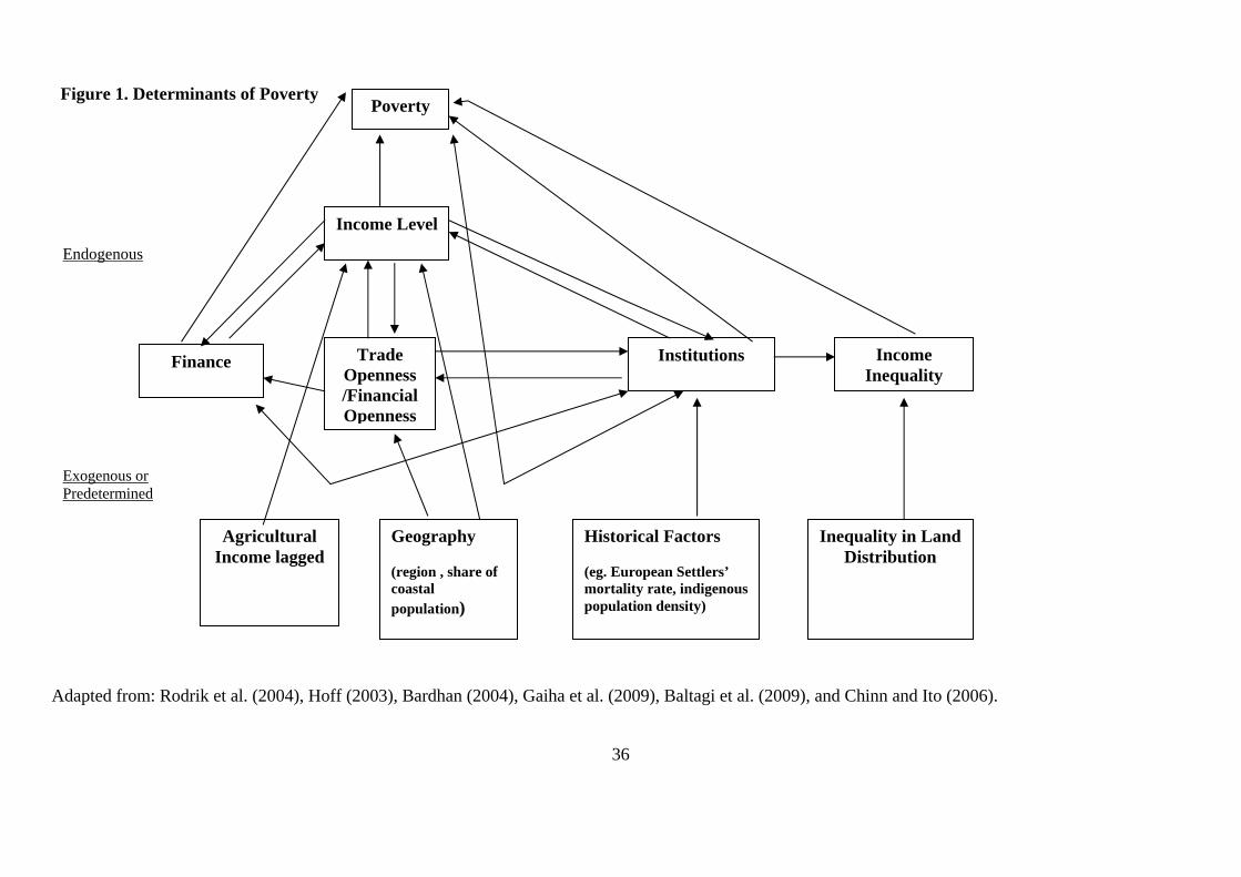
2. Analytical Framework
Our analytical framework extends Gaiha and Imai (2006) by incorporating the role of finance
in economic growth. Figure 1 provides a schematic description of the integrated framework.
We have first identified a set of predetermined and exogenous factors- namely (i) lagged
agricultural income, (ii) geography, (iii) historical factors, and (iv) inequality in land
distribution. They are shown at the bottom of the diagram. Agricultural income (or
agricultural value added per capita) 5 years ago is used as a predetermined variable to
estimate current income (or GDP per capita) to examine the effect of agricultural sector on
overall economic growth. Factors associated with geography (e.g. regional effects and the
share of coastal population) are exogenous and are supposed to affect integration (i.e. trade or
financial openness) and income level (GDP per capita). Historical factors and inequality in
land distribution are discussed below.
(Figure 1 to be inserted around here)
There are two sets of key endogenous factors that would affect income and poverty,
namely (i) institution and (ii) integration. They are shown in the middle tier of Figure 1. They
6
are likely to be endogenous given the reverse causality in the system. For example, at higher
level of income, a country can more easily form a better institution, integrate with the rest of
the country through trade or investment. Also, the pattern of economic growth would affect
income distribution.
First, institutional evolution of the country and thus the current institutional quality (e.g.
rule of law) is shaped by historical factors, such as European settlers’ mortality rate in 1500,
and indigenous population density in the same year shape (see Acemoglu et al., 2001, 2002).
Acemoglu et al. (2001, 2002) emphasise that European settlers’ mortality rates influenced
their settlement patterns and the latter resulted in the transplantation of effective European
institutions constraining the executive. When they did not settle, they instituted systems of
arbitrary rule and expropriation of local populations. What also influenced their decision to
settle was the indigenous population density (i.e. a preference for low density areas). Glaeser
et al. (2004), however, offer a different perspective on European settlement patterns, which
rests on the primacy of human and social capital in the growth process, and a second order
effect, through the latter, on institutional changes.
Integration is defined as trade openness (measured as ratio of trade to GDP) which is
linked to share of coastal population and the size of the country. Rodrik et al. (2002) report a
significant effect of institutional quality (measured in terms of property rights and rule of
law) on integration as well as a positive effect of integration on institutional quality. We also
consider the effects of ‘financial openness’ as a determinant of finance which is likely to
affect economic growth, while economic growth in turn shapes financial development.
Finance is thus treated as endogenous in the income equation and is instrumented by financial
openness and trade openness, following Baltagi et al. (2009). They used two measures of
financial openness: the Chinn and Ito (2006) index of capital account liberalisation2 and the
Lane and Milesi-Ferretti (2007) index of financial globalization (i.e. the ratio of a country's
7
foreign assets and liabilities to GDP). While the former may suffer from measurement error
in that some of the variation in the underlying economic variables may not be accounted for
(Baltagi et al., 2009), we use this because of the larger coverage of countries. Also, the results
of Chinn and Ito (2006) are important in our context because they showed that a higher level
of financial openness spurs equity market development only if a threshold level of legal
development has been attained (i.e, in many LDCs with underdeveloped legal institutions,
financial openness does not contribute to equity market development). This study also
incorporates the interrelationship between finance and economic development, both of which
are treated endogenous in the system of equations.
The third endogenous variable is income inequality, postulated as determined by
inequality in land. Income inequality is a major determinant of poverty. It could affect
income level through higher savings or indirectly as a measure of distribution of economic
power. Inequality in land distribution is considered to be exogenous because of the slow
adjustment of land market and thus could be used as a determinant of income inequality.3
3. Data
Our poverty data are based on the new World Bank head-count estimates prepared by Chen
and Ravallion (2008), with US $1.25 per day in 2005 PPP (purchasing power parity) as the
poverty line. They are taken from the World Bank’s data website called Povcal Net. 4
Although the benchmark for the MDG has been the old version of World Bank poverty
estimates with US$ 1.08 per day in 1993 PPP, it is likely that the considerably higher new
poverty estimates will trigger a debate on the feasibility of this goal. The number of countries
initially included is 115, but due to the limited coverage of key explanatory variables, the
number of countries used for estimation varies with the specification. Another difficulty is
that the new poverty estimates are highly unbalanced in the sense that the number of years for
8
which estimates are available varies across countries. So we take two different approaches.
First, we aggregate the poverty and other data and for three periods, 1980-1989, 1990-1999,
and 2000-2006 and apply the system equation estimator (namely, 3SLS). Our key variables
include institutional quality, trade share, and finance –each is treated as endogenous. As some
of the variables (e.g. agricultural value added per capita or financial openness) are lagged, we
use only two sets of the cross sectional data for 1990-1999 and 2000-2006 for which the lags
are the data pooled for 1980-1989 and 1990-1999, respectively. As an extension, these two
rounds are pooled as a panel to take account of time series changes of the variables over the
decades. Secondly, we construct annual panel data set for the entire period 1980-2006, which
are highly unbalanced because of the missing observations of poverty data. While caution is
required in interpreting the results from the unbalanced panel, the advantages are the use of a
larger data set and the probe into the time-series dimension of poverty.
Other relevant data (e.g. income per capita, agricultural value added, country size
estimates) were obtained from the World Development Indicator (WDI) 2008 (World Bank,
2008). Poverty headcount ratios and the MLD (Mean Logarithmic Deviation) Index of
income inequality have been obtained from Povcal Net. Most of the variables cover the
period from 1980 to 2006.
Institutional data were taken from the World Bank’s World Governance Indicators. Out of
the six indicators available for 1998-2007, we use ‘Voice and Accountability’, ‘Political
Stability and Absence of Violence’, ‘Rule of Law’ and ‘ Control of Corruption’. To match
the WDI data, we do not use the variable in 2007- so the data cover 1998, 2000, 2002, 2003,
2004, 2005 and 2006. The methodologies used for constructing the institutional indicators are
discussed in Kaufmann et al. (2008).5
As a proxy for the country’s financial development, we use (logarithm of) the share of
private credit as a share of GDP, an updated version of Beck et al. (2000). Following Baltagi
9
et al. (2009) we have used Chinn and Ito (2006) index of capital account openness as a
measure of financial openness.6
4. Econometric Specifications
The specifications we use are extensions of Gaiha and Imai (2006). Definitions of the
variables and names of the countries are listed in Appendix.
3SLS for cross sectional data and pooled data
For cross sectional data for 1990-1999 (or the data for 2000-2006), 3SLS is applied. As an
extension, the cross sectional data in 1990-1999 and those in 2000-2006 are pooled into a
panel to take account of the long term changes of variables over time. To make comparisons
with cross- sectional regression results by 3SLS, we apply 3SLS by using the same
specifications for the pooled data by inserting a time dummy for 2000-2006 in each equation.
County fixed effects are not considered; only regional dummy variables are used to
incorporate the regional effects. In all the cases except the dynamic panel model presented in
Table 4, the regressions are weighted by population to take into account of the fact that a
larger country, such as India, would have a larger impact on the feasibility of achieving MDG
than a small country.
First, the income equation is specified as:
i1i16i15i41i31i211t,i1101i eDIFMOAY +β+β+β+β+β+β+β= − (1)
where 01β is a constant term, iY is log of GDP per capita in t, 1990-99 (or 2000-2006) for the
i-th country. 1t,iA − is log of agricultural value added in the precious period, t-1, 1980-89 (or
1990-1999), posited to capture its long-term role in determining overall income. iO is a
measure of openness in terms of log of share of imports and exports in GDP. iM is an MLD
index of income inequality, the mean log deviation, that is, the mean across the population of
10
the log of the overall mean divided by individual income.7 iF is log of ratio of private credit to
GDP as a measure of financial development. iI represents institutional development,
designed to capture the influence of political stability, voice and accountability, control of
corruption, the rule of law, or average of these four indicators (i.e. an aggregate institutional
measure) in determining cross-country differences in income.8 iD is a vector of five regional-
level dummy variables for six regional categories, East Asia, South Asia, Sub Saharan Africa,
Latin America and Caribbean, East Europe & Central Asia, and Middle East & North Africa.
ie1 is an error term that is assumed to be independent and identically distributed (i.i.d.).
As emphasised earlier, iO and iF are likely to be endogenous. Further, it is posited that iO
also depends on the quality of institutions and some exogenous factors.
i2i32i22i1202i eCSIO +β+β+β+β= (2)
Accordingly, in equation (2), the log of trade share ( iO ) is estimated by an institutional
measure, iI and two instruments (or exogenous factors) viz. a measure of physical isolation,
iS , and country size (i.e. surface area), iC . 9 02β is a constant term and ie2 is an i.i.d error
term.
The institution equation is specified as
i3i1303i eEI +β+β= (3)
where the institutional measure is instrumented by the log of European settlers’ mortality rate,
iE , 03β is a constant term and ie3 is an i.i.d error term. As institutional indices are available
only for 1996-2006, we use the average of 1996 and 1998 values as a proxy for the
institutional quality in t, 1990-1999. For t+1, 2000-2006, we average of 2000, 2002, 2003,
2004, 2005, and 2006 values.
The poverty equation is specified as given below:
11
i4i54i44i34i24i1440i eFIDMYP +β+β+β+β+β+β= (4)
where iP is the poverty head count ratio, based on the new estimates by Chen and Ravallion
(2008) at US$1.25-a-day poverty line adjusted by PPP in 2005 10.. iM is an MLD index of
income inequality. iF is log of the ratio of private credit to GDP. We examine the direct
effect of finance on poverty by this equation as well as the indirect effect of finance on
poverty through income using both equations (1) and (4) in line with Beck et al. (2007) and
Claessens and Feijen, (2006). 04β and ie4 are the constant and error terms, respectively.
The finance equation is specified as:
i6i561t,i1t,i461t,i361t,i261t,i1606i eIK*OKOYF ++++++= −−−−− ββββββ (5)
in line with the idea that financial development is affected by economic growth, trade
openness, 1t,iO − , capital account openness or financial globalisation 1t,iK − , their interaction,
1t,i1t,i K*O −− , and institutional quality such as the rule of law.
As some of the variables- in particular, European settler’s mortality rate covers only a
limited number of countries, we have tried two different specifications- the full specification
with all five equations and the parsimonious specification with only the income equation, (1)
and the poverty equation (4) to include as many countries as possible. Note that estimating
fewer equations has the advantage of covering more countries while some of the potentially
endogenous variables are treated as exogenous variables.11
Panel Data Models
Next, to analyse the time-series changes of variables more closely, we use the annual panel
data to estimate the parsimonious specification with only the income equation, (1) and the
poverty equation (4), using random-effects IV model based on G2SLS (Generalised Two
12
Stage Least Squares). Dynamic panel data model is also estimated for finance separately to
identify the determinants of financial development.
First, we estimate random effects IV model for panel data, based on G2SLS or
Varadharajan-Krishnakumar’s (1987) estimator to estimate log of poverty headcount. In the
first stage, log of GDP per capita is estimated by instruments (e.g. lag of agricultural value
added in the previous year and trade openness) as well as the unobservable individual effect
specific to each country and year dummies (i.e. by one-way error component model). In the
second stage, log of poverty head count ratio is estimated with the individual effect and year
dummies by 2SLS where log of GDP per capita is treated as an endogenous variable.12 The
choice between fixed effects 2SLS model and random effects 2SLS model is based on the
Hausman test that compares the coefficient estimates of these models.
Following Baltagi et al. (2009), we have used a dynamic model along the lines of Blundell
and Bond (1998) to see the dynamic relationship between economic growth and financial
development. Given the possible persistence of finance, a dynamic model can be specified by
including the first lag of the dependent variable.13
it7ii581ti1it581it481ti381ti821it8108it eDK*OKOYFF +μ+β+β+β+β+β+β+β= −−−−−−
(6)
The key variables in the equation (6) are lagged trade openness, 1tiO − , lagged financial
openness, 1itK − , and their interaction, 1ti1it K*O −− . By including the interaction, Baltagi et
al. (2009) tested Rajan and Zingales’s (2003) openness hypothesis (2003) that the
simultaneous opening of both trade and capital accounts is necessary for financial
development. This is examined by testing whether the coefficients of 1tiO − , 1itK − , and
1ti1it K*O −− are all positive. However, if, for example, an economy is not open to trade as in
13
many developing countries, the coefficient of financial openness, 1itK − is expected to be
negative or zero.
Assuming that ite7 is not serially correlated and that the regressors are weakly exogenous,
the GMM first difference estimator (e.g. Arellano and Bond, 1991) can be used. Alternatively,
we could use the lagged differences of all explanatory variables as instruments for the level
equation and combine difference and level equations in a system. The panel estimators use
instrument variables based on previous realisations of the explanatory variables as the
internal instruments as in the Blundell-Bond (1998) system GMM estimator requiring
additional moment conditions. Such a system gives consistent results under the assumptions
that there is no second order serial correlation and the instruments are uncorrelated with the
error terms. Validity of instruments is tested by the Sargan J test and the second order serial
correlation of the residuals. The Blundell-Bond (1998) system GMM estimator is used in the
present study.
5. Econometric Results
Tables 1 and 2 give the results of 3SLS applied to cross-sectional and pooled data for 1990-
1999, 2000-2006 and 1990-2006, and Tables 3 to 4 give those based on panel data models.
For each table, five different measures of institutional index are used separately in each
specification. Key variables we are interested in are shown in bold figures.
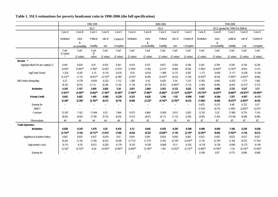
Table 1 shows the results based on 3SLS applied to all five equations. In all fifteen cases
(five cases for 1990-1999, 2000-2006 and 1990-2006), the effect of institutions on income is
positive and significant. However, some caution is necessary as European settlers’ mortality
rate has a negative and significant effect only on rule of law (Case D) and control of
corruption (Case E) in 2000-2006, voice and accountability (Case B) and rule of law (Case
14
D) in 1990-2006. The coefficient of agricultural value added in the previous decade is
positive and mostly significant for 1990-1999, positive and significant only for Cases A and
C for 2000-2006, and positive and significant for Cases A, B and C for 1990-2006. This is
consistent with the role of agricultural sector in promoting economic growth in the long run.
Trade openness, which is instrumented by the physical isolation index and the country size, is
either ‘negative and significant’ or non-significant. This looks counter-intuitive, but is
consistent with earlier studies, such as Rodrik et al. (2004) and Gaiha and Imai (2006), which
showed that trade openness does not have any impact on income or income growth once the
openness is instrumented by institutional qualities.
(Table 1 to be inserted around here)
Our results obtained from the trade openness equation suggest that political stability,
among the four institutional variables, is the most important determinant of trade openness.
The positive and highly significant coefficient suggests that the higher the political stability
the greater is trade openness. The rule and law is important only for 1990-1999 as its
coefficient is positive and significant at the 10% level, while it is non-significant for 2000-6.
Physical isolation index has an (expected) positive sign and is significant for 2000-2006.14
Log of surface area has an (expected) negative and significant coefficient at the 5 % level
except in Case C for 1990-1999.
In the poverty equation, MLD index, a measure of inequality, is positive and significant at
the 5 % significance level in most cases.15 It is noted that the coefficient estimate of MLD
index is almost twice larger in 2000-2006 than in 1990-1999. The effect of inequality is more
pronounced to influence poverty after 2000- which could reflect the fact that the countries
with relatively large poverty indices after 2000 tend to be characterised by higher income
inequality.
15
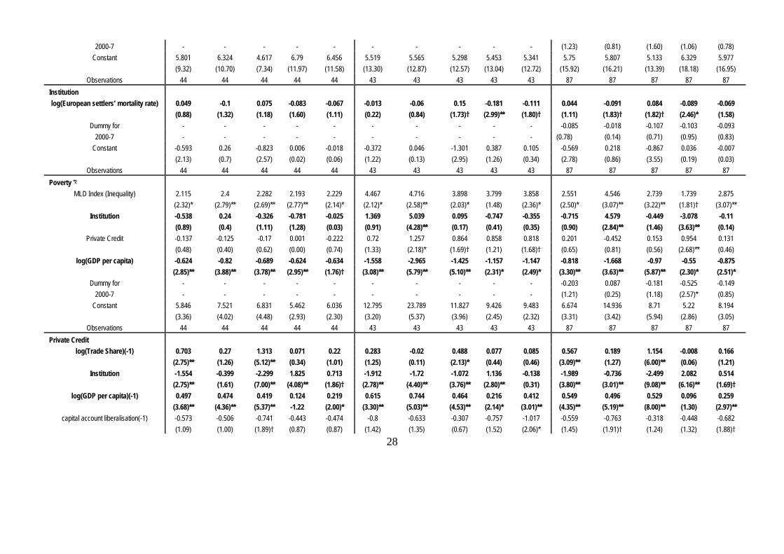
The coefficient estimate of log of GDP per capita measures the elasticity of poverty with
respect to GDP per capita (i.e. percentage change of poverty headcount ratio corresponding to
1 % change of GDP per capita).16 It is negative and significant in all cases. Comparison of the
coefficients for 1990-1999 and 2000-2006 brings out the change of the elasticity before and
after 2000. Table 1 shows that the elasticity of poverty head count ratio with respect to GDP
per capita was larger (in absolute terms) after 2000. However, the change of elasticity is
sensitive to (i) the specification, (ii) sample of countries included and (iii) the change of the
coefficient of correlation between log GDP per capita and an MLD index before and after
2000 (0.06 versus 0.14). To make Table 1 and Table 2 comparable, we have tried the
parsimonious specification (with only income and poverty equations) for the smaller set of
countries used for the full specification. The columns labelled as Case A’ in Table 2 presents
the results for a smaller countries based on the parsimonious specification where the
aggregate institution measure is used. The elasticity of poverty head count ratio with respect
to GDP per capita (in absolute values) declined from 1.77 to 1.27 after 2000. Besides, if we
compare the corresponding coefficients for 1980-99 and 2000-2006 based on annual panel
data in Table 3 (in the second panel of Case B and Case C), there was a marked reduction in
the poverty elasticity- from -1.50 for 1980-1990 to -1.08 for 2000-2006. We are inclined to
prefer this finding mainly because the sample is larger, while we note the limitation that this
is based on Tables 2 and 3, not on Table 1.
The coefficient estimate of private credit is positive and significant in Cases B, C and D
for 2000-2006 or non-significant for 1990-1999 in the poverty equation in Table 1. However,
it should be noted that the overall impact of private credit on poverty is the combination of
the indirect effect through income and the direct effect through consumption smoothing. The
indirect effect through income is negative if credit has a positive and significant effect on
income because income is negative and significant in the poverty equation. For example, in
16
Case B and Case C for 2000-2006, the overall effect of finance on poverty is negative as the
negative indirect effect as a multiplication of income elasticity with respect to finance (-1.692
in Case B and -1.921 in Case C respectively) is larger than the direct effect as poverty
elasticity with respect to income (1.257 and 0.864 respectively).
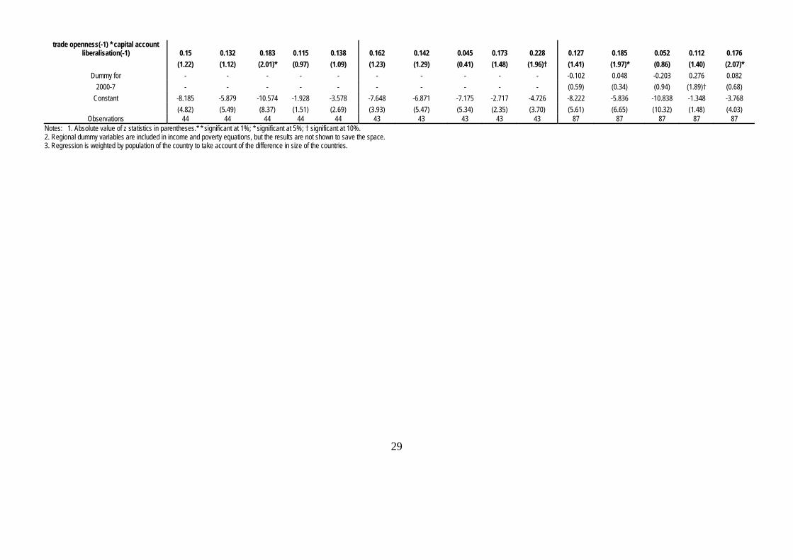
The finance equation also has different results depending on the period or on which
institutional variable is used. The coefficient of institution is either positive and significant or
negative and significant depending on which governance indicator is used. Interestingly, the
rule of law and the control of corruption have the right (or positive) sign with significant
coefficients for 1990-1999 and 1990-2006. Trade openness affects private credit positively
with one-period lag as the coefficient in question is positive and significant in Cases A and C
for 1990-1999 and 1990-2006. Lagged log of GDP per capita has mostly a positive and
significant effect. Capital account liberalisation with one period lag has a negative but mostly
non-significant effect except several cases, that is, Case C for 1990-1999, Case E for 2000-
2006 and Cases B and E for 1990-2006. In these cases, the interaction of trade and financial
openness affects private credit positively.
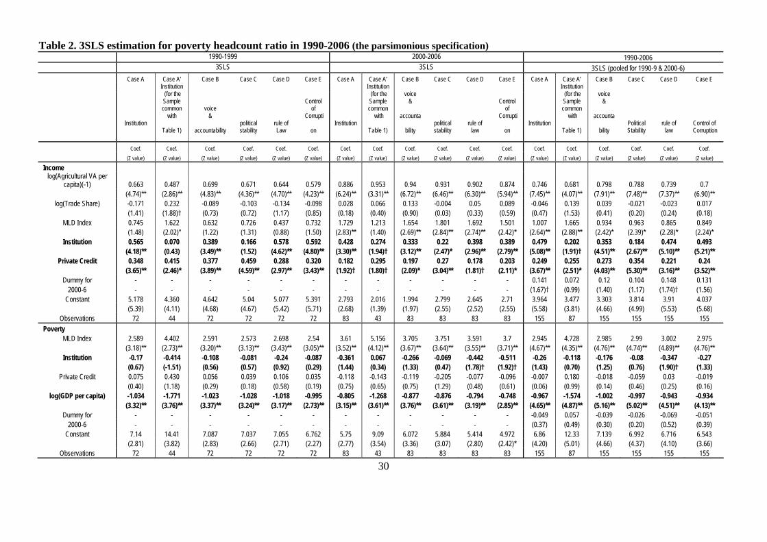
The results presented in Table 2 are based on the simplest specification whereby income
and poverty are estimated by 3SLS. 72 (83 or 155) countries are covered for 1990-1999
(2000-2006 or 1990-2006). In the first panel for the income equation, the coefficient estimate
of (uninstrumented) institutions is positive and significant at the 1 % level for all cases except
Case C for 1990-1999. The second panel for the poverty equation shows that the coefficient
estimate of institution is not significant except in Case D (the rule of law) and Case E (control
of corruption) for 2000-2006 and Case D for 1990-2006 with the coefficient estimate
negative and significant coefficients at the 10 % level. Private credit is non-significant for
poverty in any of fifteen cases while it is positive and significant for log of GDP per capita.
Log of GDP per capita has a highly significant negative effect on poverty that has weakened
17
over 2000-2006. That is, the elasticity of poverty with respect to GDP per capita changed
from around -1 in 1990-1999 to -0.75 to -0.88 in 2000-2006. The effect of the MLD index of
income inequality is positive but stronger in 2000-2006 than in 1990-1999. Also, there is a
dilution of the indirect effect of institutional quality through income in the more recent period.
The columns labelled as Case A’ in Table 2 show the results for the aggregate institution
which are applied to the smaller sample common with Table for 1990-1999, 2000-2006 and
1990-2006. If we compare these cases with the corresponding cases (Case A) in Table 1, we
find the pattern of the results in terms of significance and signs of coefficient estimates are
similar with a few changes (e.g. for income in Table 2, institution is not significant or trade
openness is positive and significant in 1990-99). As we noted, poverty elasticity with respect
to income declined after 2000 with larger absolute values in Case A’ of Table 2, while it
increased in Case A of Table 1. Case A and Case A’ of Table 2 also show the similar pattern
of the results with a few exceptions (e.g. institution is not significant in Case A’ 1990-99).
(Table 2 to be inserted around here)
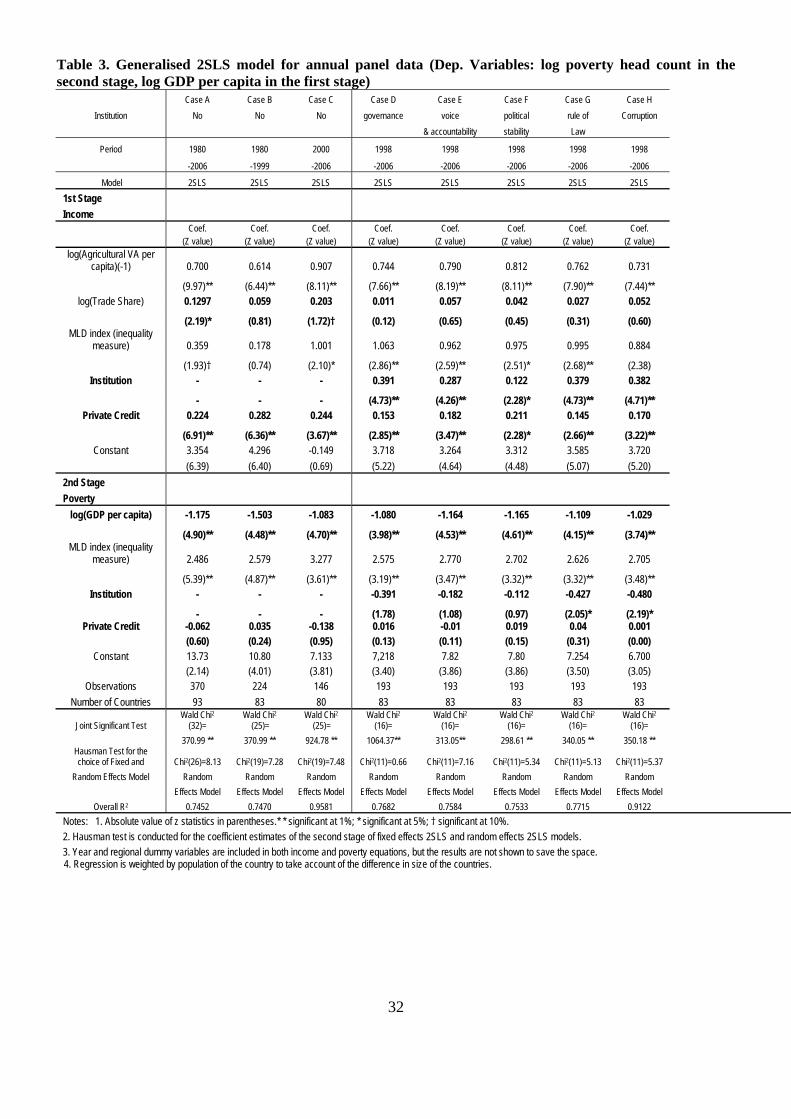
Table 3 presents the results based on G2SLS applied for annual panel data where log of GDP
per capita is estimated in the first stage and log of poverty head count ratio is estimated in the
second stage. First, we have carried out three regressions for 1980-2006, 1980-1999, and
2000-2006 without institutions in order to have a larger number of observations (because
institutional indicators are only available in 1996-2007), the results of which are shown in the
first three columns, Cases A, B and C. The number of countries is 83 or 93. Then, five
measures of institutional variables are inserted without being instrumented in Cases D to H.
In this analysis, 83 countries are included.
Most of the results are expected and are broadly consistent with those in Table 2 with a
few differences. Log of trade share has a positive and significant effect on log GDP per capita
18
at the 5 % level in Case A (full period) and at the 10 % in Case C (2000-2006), but it is not
significant in other cases. Institutions, however, have positive and significant effects in all the
cases. Private credit has a positive and highly significant effect, as in Table 2.
(Table 3 to be inserted around here)
As we have already noted, we observe in the second panel of Table 3 that the elasticity of
poverty with respect to GDP per capita declined in absolute values i.e., from -1.50 for 1980-
1999 to -1.08 for 2000-2006. For the full period, the elasticity is -1.28. While the MLD index
of income inequality has a positive and significant effect on poverty, the elasticity is higher in
the more recent period. However, private credit does not have a significant effect on poverty.
In other words, the indirect effect of credit though income is dominant and the direct effect is
negligible. Better institution in terms of the rule of law (Case G) and control of corruption
(Case H) tend to significantly reduce poverty at the 5 % level. Aggregate institutional quality
(Case D) is negative and significant at the 10% significance level. The total effect of
institutions through income and directly on poverty is found to be substantial.
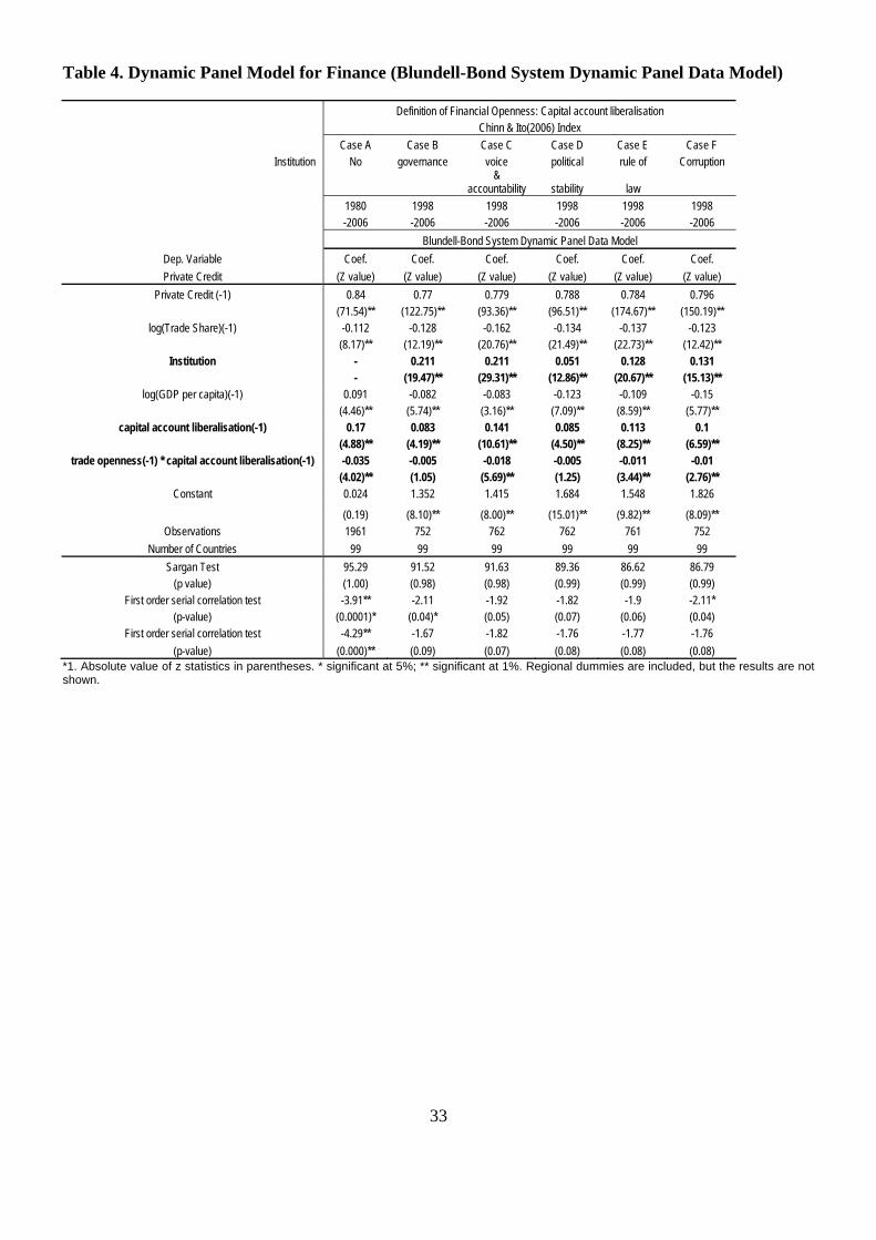
Table 4 gives the results of dynamic panel data model based on Blundell-Bond GMM
estimator to identify more clearly the relationship between economic growth and financial
development. This is a direct extension of Baltagi et al. (2009), but we have used institution
as one of the determinants of private credit. 17 Lagged GDP per capita is positive and
significant in Case A where institution is not included (for 1980-2006). However, it is
negative and significant in Cases B to F where institution is used as one of the explanatory
variables (for 1998-2006). Lagged trade openness has a negative and significant effect in all
the cases, that is, the more open the country is to the rest of the world, the financial
development is hindered to a larger extent. This may be because when an economy opens up
to trade with its capital account closed, as suggested by Rajan and Zingales (2003), there will
19
be calls for additional financial repression to protect industrial incumbents, which would
prevent financial development from taking off (see Baltagi et al., 2009). Institutions, however,
have a positive and significant effect in all cases. Lagged capital account liberalisation has a
positive and highly significant effect while the interaction term of lagged trade openness and
lagged capital account liberalisation has a negative and significant coefficient. If private
credit is an appropriate proxy for the financial sector development, our results by and large
suggest that capital account liberalisation, economic growth and institutional development are
among the key factors for the country’s financial development. A future research using the
longer time series or panel data based on a more comprehensive set of variables would be
required to confirm this conclusion.
(Table 4 to be inserted around here)
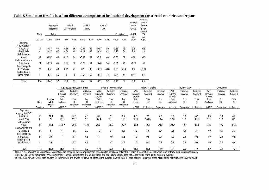
6. Simulation Results
Table 5 reports simulation results, based on Generalised 2SLS model (or static annual panel
data model) whereby log of GDP per capita and log of poverty headcount ratio are estimated
in Case D to Case H in Table 3. The reason for using static annual panel data model is that
we can take into account the annual change of institutional qualities or other key variables.
This would enable us to make prediction of poverty ratios in 2015 more easily.
The purpose of the simulation is to examine whether change of institutional quality would
affect poverty or the prospect of halving poverty. This is a simple linear prediction of the
future value of log of poverty head count ratio (that will be converted to poverty head count
ratio) in 2015, obtained from the static linear panel data regression results during 1998-2006,
under the following assumptions: (i) annual growth rates of GDP per capita and agricultural
value added per capita will be same in 2007-2015 as their historical averages of 1980-2006;
(ii) the MLD index of income inequality and trade share will remain same as the levels in
20
2006 till 2015; and (iii) private credit will remain same as the minimum level in 2000-2006
(to reflect the recent contraction of finance). Three institutional scenarios are combined with
the preceding assumptions: (i) institutional qualities continue to be same as the level in 2006;
(ii) they improve to the average of top 30 countries by 2015; (iii) and they rise to the average
of top 10 countries by 2015. Simulations have been carried out for six regions and total of
developing countries.
(Table 5 to be inserted around here)
Our calculation shows that MDG1 for all developing countries based on the new poverty
data is 17.3%, taking the average weighted by population of each country. The simulation
results will have to be interpreted with caution given that the changes in the poverty
headcount ratio are based on the linear prediction and are far from small. It is also noted that
China is not included in our simulations because it lacks the private credit data. If the
historical growth rate is kept for each country, the estimated poverty head count ratio is
15.7%, which is lower than the MDG of 17.3%. So it would be possible to achieve the MDG
if the historical annual economic growth rate is maintained at the country levels. An
exception is Sub-Saharan Africa. Sub-Saharan Africa’s initial level of poverty head count
ratio is high at 50.6% in 1990 and it reduces to barely 34% in the basic scenario, much higher
than the target of 25.3%. Latin America’s initial poverty ratio was as low as 12% in 1990,
but it would not achieve MDG1 (or 6% in 2015) because its expected poverty ratio is 7.0% to
7.3 %, above the target, under the assumptions that historical growth rate would continue and
institutional qualities would be unchanged at the level in 2006.
All the other regions will meet MDG1 in the sense that predicted poverty head count ratio
is less than half of that in 1990. In the scenario where all the countries improve their
institutional qualities to the average of top 30 countries, all developing countries and all the
21
regions will meet the MDG1 because of the dramatic effect of the improvement in
institutional qualities on poverty reduction (through both indirect and direct channels). Of
particular interest is the case where rule of law or control of corruption improves. If, for
example, the rule of law improves to the level of top 30 performers, the predicted poverty
head count ratio will reduce from 15.4% to 9.0%. For Sub-Saharan Africa, the improvements
in the rule of law or control of corruption have the potential of reducing poverty drastically.
Assuming the average of top 30 performers in terms of the rule of law or the control of
corruption, Sub-Saharan Africa will halve poverty by 2015. Simulations at regional levels
show that improvement in institutional quality is crucial to poverty reduction.
7. Concluding Remarks
The present study has examined the prospect of achieving the Millennium Development Goal
(MDG) of income poverty using Chen and Ravallion’s (2008) new international poverty
estimates with a particular focus on the role of institutions, such as voice and accountability
or rule of law, income growth and agricultural income growth, change in income inequality
and finance. Our main findings are summarised below.
First, better institutions are associated with i) higher income levels of the country
(irrespective of the definition of institution); ii) higher levels of trade openness; iii) lower
level of poverty (for the cases of better rule of law and control of corruption); and iv) higher
level of financial development (in the cases of better rule of law or control of corruption for
cross sectional regression; in all the cases for dynamic panel data model). These results are
important as institutions are treated as an endogenous variable in one of the specifications.
The indirect effect of improvements in institution on poverty reduction through finance, trade
openness and income matters is thus important.
22
Second, there are strong interrelationships between financial development and economic
development as suggested by the cross-sectional regressions. The positive association of
private credit and lagged GDP per capita is also observed by the dynamic panel data model
applied for 1980-2006. What is important, though, is that for developing countries, trade
openness alone may not help developing finance; lagged capital account openness and better
institutional quality have more important roles in financial development as suggested by the
dynamic panel data model.
Third, our simulations show that, if the historical economic growth rate is maintained,
MDG1 will be feasible. However, disaggregation of the simulation results by region shows
that Sub-Saharan Africa will be unable to meet this goal without a substantial improvement in
its institutional quality, for example, without better rule of laws or better control of corruption.
In general, improvement in institutional quality or reduction in income inequality is crucial to
achieving MDG1.
Some other valuable insights have also emerged from the present analysis. The first
important insight is that the elasticity of poverty with respect to income has reduced (in
absolute terms) in recent years. Another insight drawn from some of our econometric results
is that the positive (conditional) association between poverty and income inequality tends to
be larger in more recent years. Finally, there are a few cases of the weakening of the effect of
institutional quality on poverty indirectly through income, finance and trade openness as well
as directly via smoothing of consumption.
References
Acemoglu, D., Johnson S. & Robinson, J. A. (2001) The Colonial Origins of Comparative
Development: An Empirical Investigation, American Economic Review, 91(5), pp.1369-
1401.
23
Acemoglu, D., Johnson, S. & Robinson, J. A. (2002) Reversal of Fortune: Geography and
Development in the Making of the Modern World Income Distribution, Quarterly Journal
of Economics, 117(4), pp.1231-1294.
Acemoglu, D., Johnson, S. & Robinson, J. A. (2005) A Response to Albouy’s A
Reexamination Based on Improved Settler Mortality Data, Draft, March, 2005.
Arellano, M. & Bond, S. (1991) Some tests of specification for panel data: Monte Carlo
evidence and an application to employment equations, Review of Economic Studies, 58,
pp.277-297.
Baltagi, B. H. (1981) Simultaneous equations with error components, Journal of
Econometrics, 17, pp.189–200.
Baltagi, B. H. (2005) Econometric Analysis of Panel Data, Third Edition (Chichester:, John
Wiley & Sons Ltd.).
Baltagi, B.H., Demetriades, P. O. & Law, S. H. (2009) Financial development and openness:
Evidence from panel data, Journal of Development Economics, 89 (2), July 2009, pp. 285-
296.
Balestra, P. & Varadharajan-Krishnakumar, J. (1987) Full information estimations of a
system of simultaneous equations with error components structure, Econometric Theory 3,
pp. 223–246.
Bardhan, P. (2004) Scarcity, Conflicts, and Cooperation: Essays in the Political and
Institutional Economics of Development (Cambridge, MIT Press).
Beck, T., Demirgüç-Kunt, A. & Levine, R. (2000) A New Database on Financial
Development and Structure, World Bank Economic Review 14, pp.597-605.
Beck, T., Demirguck-Kunt, A. & Levine, R. (2007) Finance, Inequality and the Poor, Journal
of Economic Growth, 12, pp.27-49.
24
Besley, T. & Burgess, R. (2003) Halving Global Poverty, Journal of Economic Perspectives,
17(3), pp.3-22.
Blundell, R. & Bond, S. (1998) Initial conditions and moment restrictions in dynamic panel-
data models, Journal of Econometrics 87, pp.115-143.
Chen, S. & Ravallion, M. (2008) The Developing World Is Poorer Than We Thought, But No
Less Successful in the Fight against Poverty, Policy Research Working Paper WPS 4703,
(Washington D.C., World Bank).
Chinn, M.D. & Ito, H. (2006) What matters for financial development? Capital controls,
institutions and interactions, Journal of Development Economics, 81, pp.163–192.
Claessens, S. & Feijen, E. (2006) Finance and Hunger: Empirical Evidence of the
Agricultural Productivity Channel, World Bank Policy Research Working Paper 4080,
December 2006, Washington D.C. World Bank.
Deininger, K. & Squire, L. (1998) New ways of looking at old issues: inequality and growth,
Journal of Development Economics, 57, pp.259-287.
Demery, L. & Walton, M. (1999). Are Poverty and Social Goals for the 21st Century
Attainable? IDS Bulletin, 30(2), pp.75-91.
Gaiha, R. & Imai, K. (2006) Do Institutions Matter in Poverty Reduction? Prospects of
Achieving the MDG of Poverty Reduction in Asia, Statistica & Applicazioni, IV(2), pp.29-
160.
Gaiha, R., Imai, K. & Nandhi, M.A. (2009) Millennium Development Goal of Halving
Poverty in Asia and the Pacific Region: Progress, Prospects and Priorities, Journal of Asian
and African Studies, 44(2), pp.215-237.
Glaeser, E. L., Porta, R. L., Lopez-De-Silanes, F., Shleifer, A. (2004) Do Institutions Cause
Growth? Journal of Economic Growth, 9, pp.271-303.
Greene, W. (2000) Econometric Analysis- Fourth Edition (New Jersey, Prentice Hall Inc.).
25
Guariglia, A. & Poncet, S. (2008) Could Financial Distortions be no Impediment to
Economic Growth After All? Evidence from China, Journal of Comparative Economics,
36(4), pp.633-657.
Heltberg, R. (2002) The Poverty Elasticity of Growth, WIDER Discussion Paper 2002/21
(Helsinki, UNU-WIDER).
Hoff, K. (2003) Paths of Institutional Development: A View from Economic History, World
Bank Economic Review, 18(2), pp.2205-226.
Kaufmann, D., Kraay, A., & Mastruzzi, M. (2008) Governance Matters VII: Aggregate and
Individual Governance Indicators, 1996-2007, World Bank Policy Research Working Paper
No. 4654 (Washington D.C., The World Bank).
Lane, P. R & Milesi-Ferretti, G. M. (2007) The external wealth of nations mark II: Revised
and extended estimates of foreign assets and liabilities, 1970–2004, Journal of International
Economics, 73 (2), pp.223-250.
McArthur, J. & Sachs, J. W. (2002) A Millennium Development Strategy for Achieving
Poverty Alleviation and Economic Growth, Draft.
Rajan, R.G. & Zingales, L. (2003) The great reversals: the politics of financial development
in the twentieth century, Journal of Financial Economics, 69, pp.5–50.
Ravallion, M., Chen, S., & Sangraula, P. (2008) Dollar a Day Revisited, World Bank Policy
Research Working Paper No. 4620 (Washington D.C., World Bank).
Rodrik, D., Subramanian, A. & Trebbi, F. (2004) ‘Institutions Rule: The Primacy of
Institutions over Integration and Geography in Development’, Journal of Economic Growth,
9, pp.131-165.
United Nations. (2003).Promoting the Millennium Development Goals in Asia and the
Pacific, (New York, United Nations).
26
United Nations (2008) The Millennium Development Goals Report 2008, (New York, United
Nations).
World Bank (2008) World Development Indicators, (Washington D.C., Oxford University
Press).
27
Table 1. 3SLS estimations for poverty headcount ratio in 1990-2006 (the full specification)
1990-1999 2000-2006 1990-2006 3SLS 3SLS 3SLS (pooled for 1990-9 & 2000-6)
Case A Case B Case C Case D Case E Case A Case B Case C Case D Case E Case A Case B Case C Case D Case E
Institution voice Political rule of Control of Institution voice Political rule of Control of Institution voice political rule of Control of &
accountability Stability law Corruption &
accountability Stability law Corruption &
accountability stability Law Corruption
Coef. Coef. Coef. Coef. Coef. Coef. Coef. Coef. Coef. Coef. Coef. Coef. Coef. Coef. Coef.
(Z value)
*1 (Z value) (Z
value) (Z value) (Z value) (Z value) (Z value) (Z value) (Z value) (Z value) (Z value) (Z value) (Z value) (Z value) (Z value) Income *2
log(Agricultural VA per capita)(-1) 0.441 0.629 0.41 0.476 0.361 0.413 0.321 0.657 0.283 0.106 0.301 0.709 0.345 0.154 0.236 (2.05)* (2.60)** (1.96)* (2.03)* (1.67)† (1.69)† (1.60) (2.51)* (0.84) (0.36) (1.80)† (2.64)** (2.76)** (0.81) (1.41)
log(Trade Share) -1.324 -0.267 -2.15 -0.716 -0.476 -0.55 -0.016 -1.489 0.175 0.387 -1.171 -0.093 -2.117 -0.528 -0.144 (5.22)** (1.13) (4.81)** (3.15)** (2.38)* (2.07)* (0.09) (4.35)** (0.52) (1.34) (5.93)** (0.54) (7.89)** (2.82)** (0.86)
MLD Index (Inequality) 0.27 -0.776 -0.854 -0.322 1.112 1.385 0.16 0.429 5.54 1.313 0.783 0.945 -0.353 1.777 1.062 (0.32) (0.91) (1.11) (0.38) (1.32) (1.14) (0.19) (0.32) (2.89)** (1.13) (1.06) (0.86) (0.69) (2.21)* (1.57)
Institution 4.245 2.157 3.605 3.826 3.34 3.921 2.669 2.553 6.123 3.035 4.747 4.688 3.732 5.527 3.17 (7.81)** (4.30)** (5.84)** (7.18)** (9.18)** (7.46)** (7.98)** (5.68)** (7.12)** (6.50)** (10.73)** (6.67)** (9.89)** (10.87)** (10.99)**
Private Credit 0.642 0.683 1.405 -0.085 -0.229 0.321 0.628 1.348 -1.93 -0.098 0.487 -0.304 1.357 -0.957 -0.112 (2.28)* (2.28)* (5.70)** (0.27) (0.74) (0.80) (2.23)* (4.14)** (2.79)** (0.23) (1.80)† (0.68) (9.47)** (2.85)** (0.43)
Dummy for - - - - - - - - - - 0.475 0.215 0.48 0.722 0.37 2000-7 - - - - - - - - - - (1.92)† (0.73) (1.89)† (2.85)** (2.07)*
Constant 12.597 7.162 17.404 8.33 7.946 9.973 6.864 13.005 3.012 5.833 12.351 3.25 17.805 8.776 7.314 (8.83) (4.82) (7.39) (5.73) (6.03) (5.51) (4.67) (6.11) (1.12) (2.90) (9.85) (1.82) (13.56) (6.68) (6.86)
Observations 44 44 44 44 44 43 43 43 43 43 87 87 87 87 87 Trade Openness
Institution 0.838 -0.247 1.479 0.55 0.416 0.13 0.045 0.478 -0.281 -0.398 0.498 -0.093 1.106 0.239 -0.036 (2.74)** (1.54) (6.71)** (1.91)† (1.60) (0.62) (0.32) (3.64)** (1.19) (2.19)* (2.59)** (0.84) (7.93)** (1.14) (0.21)
log(physical isolation index) 0.007 0.035 0.037 -0.016 0.01 0.041 0.041 0.034 0.056 0.062 0.022 0.042 0.023 0.012 0.037 (0.24) (1.16) (1.30) (0.52) (0.28) (1.71)† (1.77)† (1.65) (2.19)* (2.63)** (1.13) (2.19)* (1.34) (0.57) (1.75)†
log(country’s size) -0.115 -0.18 0.013 -0.203 -0.179 -0.101 -0.109 -0.069 -0.11 -0.102 -0.118 -0.136 -0.043 -0.172 -0.149 (2.16)* (3.75)** -0.24 (4.29)** (3.96)** (3.06)** (3.18)** -1.96 (3.35)** (3.12)** (3.98)** (4.78)** -1.34 (6.10)** (5.34)**
Dummy for - - - - - - - - - - 0.108 0.07 0.175 0.094 0.068
28
2000-7 - - - - - - - - - - (1.23) (0.81) (1.60) (1.06) (0.78) Constant 5.801 6.324 4.617 6.79 6.456 5.519 5.565 5.298 5.453 5.341 5.75 5.807 5.133 6.329 5.977
(9.32) (10.70) (7.34) (11.97) (11.58) (13.30) (12.87) (12.57) (13.04) (12.72) (15.92) (16.21) (13.39) (18.18) (16.95) Observations 44 44 44 44 44 43 43 43 43 43 87 87 87 87 87
Institution log(European settlers’ mortality rate) 0.049 -0.1 0.075 -0.083 -0.067 -0.013 -0.06 0.15 -0.181 -0.111 0.044 -0.091 0.084 -0.089 -0.069
(0.88) (1.32) (1.18) (1.60) (1.11) (0.22) (0.84) (1.73)† (2.99)** (1.80)† (1.11) (1.83)† (1.82)† (2.46)* (1.58) Dummy for - - - - - - - - - - -0.085 -0.018 -0.107 -0.103 -0.093
2000-7 - - - - - - - - - - (0.78) (0.14) (0.71) (0.95) (0.83) Constant -0.593 0.26 -0.823 0.006 -0.018 -0.372 0.046 -1.301 0.387 0.105 -0.569 0.218 -0.867 0.036 -0.007
(2.13) (0.7) (2.57) (0.02) (0.06) (1.22) (0.13) (2.95) (1.26) (0.34) (2.78) (0.86) (3.55) (0.19) (0.03) Observations 44 44 44 44 44 43 43 43 43 43 87 87 87 87 87
Poverty *2 MLD Index (Inequality) 2.115 2.4 2.282 2.193 2.229 4.467 4.716 3.898 3.799 3.858 2.551 4.546 2.739 1.739 2.875
(2.32)* (2.79)** (2.69)** (2.77)** (2.14)* (2.12)* (2.58)** (2.03)* (1.48) (2.36)* (2.50)* (3.07)** (3.22)** (1.81)† (3.07)** Institution -0.538 0.24 -0.326 -0.781 -0.025 1.369 5.039 0.095 -0.747 -0.355 -0.715 4.579 -0.449 -3.078 -0.11
(0.89) (0.4) (1.11) (1.28) (0.03) (0.91) (4.28)** (0.17) (0.41) (0.35) (0.90) (2.84)** (1.46) (3.63)** (0.14) Private Credit -0.137 -0.125 -0.17 0.001 -0.222 0.72 1.257 0.864 0.858 0.818 0.201 -0.452 0.153 0.954 0.131
(0.48) (0.40) (0.62) (0.00) (0.74) (1.33) (2.18)* (1.69)† (1.21) (1.68)† (0.65) (0.81) (0.56) (2.68)** (0.46) log(GDP per capita) -0.624 -0.82 -0.689 -0.624 -0.634 -1.558 -2.965 -1.425 -1.157 -1.147 -0.818 -1.668 -0.97 -0.55 -0.875
(2.85)** (3.88)** (3.78)** (2.95)** (1.76)† (3.08)** (5.79)** (5.10)** (2.31)* (2.49)* (3.30)** (3.63)** (5.87)** (2.30)* (2.51)* Dummy for - - - - - - - - - - -0.203 0.087 -0.181 -0.525 -0.149
2000-7 - - - - - - - - - - (1.21) (0.25) (1.18) (2.57)* (0.85) Constant 5.846 7.521 6.831 5.462 6.036 12.795 23.789 11.827 9.426 9.483 6.674 14.936 8.71 5.22 8.194
(3.36) (4.02) (4.48) (2.93) (2.30) (3.20) (5.37) (3.96) (2.45) (2.32) (3.31) (3.42) (5.94) (2.86) (3.05) Observations 44 44 44 44 44 43 43 43 43 43 87 87 87 87 87
Private Credit log(Trade Share)(-1) 0.703 0.27 1.313 0.071 0.22 0.283 -0.02 0.488 0.077 0.085 0.567 0.189 1.154 -0.008 0.166
(2.75)** (1.26) (5.12)** (0.34) (1.01) (1.25) (0.11) (2.13)* (0.44) (0.46) (3.09)** (1.27) (6.00)** (0.06) (1.21) Institution -1.554 -0.399 -2.299 1.825 0.713 -1.912 -1.72 -1.072 1.136 -0.138 -1.989 -0.736 -2.499 2.082 0.514
(2.75)** (1.61) (7.00)** (4.08)** (1.86)† (2.78)** (4.40)** (3.76)** (2.80)** (0.31) (3.80)** (3.01)** (9.08)** (6.16)** (1.69)† log(GDP per capita)(-1) 0.497 0.474 0.419 0.124 0.219 0.615 0.744 0.464 0.216 0.412 0.549 0.496 0.529 0.096 0.259
(3.68)** (4.36)** (5.37)** -1.22 (2.00)* (3.30)** (5.03)** (4.53)** (2.14)* (3.01)** (4.35)** (5.19)** (8.00)** (1.30) (2.97)** capital account liberalisation(-1) -0.573 -0.506 -0.741 -0.443 -0.474 -0.8 -0.633 -0.307 -0.757 -1.017 -0.559 -0.763 -0.318 -0.448 -0.682
(1.09) (1.00) (1.89)† (0.87) (0.87) (1.42) (1.35) (0.67) (1.52) (2.06)* (1.45) (1.91)† (1.24) (1.32) (1.88)†
29
trade openness(-1) * capital account liberalisation(-1) 0.15 0.132 0.183 0.115 0.138 0.162 0.142 0.045 0.173 0.228 0.127 0.185 0.052 0.112 0.176
(1.22) (1.12) (2.01)* (0.97) (1.09) (1.23) (1.29) (0.41) (1.48) (1.96)† (1.41) (1.97)* (0.86) (1.40) (2.07)* Dummy for - - - - - - - - - - -0.102 0.048 -0.203 0.276 0.082
2000-7 - - - - - - - - - - (0.59) (0.34) (0.94) (1.89)† (0.68) Constant -8.185 -5.879 -10.574 -1.928 -3.578 -7.648 -6.871 -7.175 -2.717 -4.726 -8.222 -5.836 -10.838 -1.348 -3.768
(4.82) (5.49) (8.37) (1.51) (2.69) (3.93) (5.47) (5.34) (2.35) (3.70) (5.61) (6.65) (10.32) (1.48) (4.03) Observations 44 44 44 44 44 43 43 43 43 43 87 87 87 87 87
Notes: 1. Absolute value of z statistics in parentheses.* * significant at 1%; * significant at 5%; † significant at 10%. 2. Regional dummy variables are included in income and poverty equations, but the results are not shown to save the space. 3. Regression is weighted by population of the country to take account of the difference in size of the countries.
30
Table 2. 3SLS estimation for poverty headcount ratio in 1990-2006 (the parsimonious specification) 1990-1999 2000-2006 1990-2006 3SLS 3SLS 3SLS (pooled for 1990-9 & 2000-6) Case A Case A’ Case B Case C Case D Case E Case A Case A’ Case B Case C Case D Case E Case A Case A’ Case B Case C Case D Case E
Institution
Institution (for the Sample common
with
Table 1)
voice &
accountability political stability
rule of Law
Control of
Corrupti
on Institution
Institution (for the Sample common
with
Table 1)
voice &
accounta
bility political stability
rule of law
Control of
Corrupti
on Institution
Institution (for the Sample common
with
Table 1)
voice &
accounta
bility Political Stability
rule of law
Control of Corruption
Coef. Coef. Coef. Coef. Coef. Coef. Coef. Coef. Coef. Coef. Coef. Coef. Coef. Coef. Coef. Coef. Coef. Coef.
(Z value) (Z value) (Z value) (Z value) (Z value) (Z value) (Z value) (Z value) (Z value) (Z value) (Z value) (Z value) (Z value) (Z value) (Z value) (Z value) (Z value) (Z value)
Income log(Agricultural VA per
capita)(-1) 0.663 0.487 0.699 0.671 0.644 0.579 0.886 0.953 0.94 0.931 0.902 0.874 0.746 0.681 0.798 0.788 0.739 0.7 (4.74)** (2.86)** (4.83)** (4.36)** (4.70)** (4.23)** (6.24)** (3.31)** (6.72)** (6.46)** (6.30)** (5.94)** (7.45)** (4.07)** (7.91)** (7.48)** (7.37)** (6.90)**
log(Trade Share) -0.171 0.232 -0.089 -0.103 -0.134 -0.098 0.028 0.066 0.133 -0.004 0.05 0.089 -0.046 0.139 0.039 -0.021 -0.023 0.017 (1.41) (1.88)† (0.73) (0.72) (1.17) (0.85) (0.18) (0.40) (0.90) (0.03) (0.33) (0.59) (0.47) (1.53) (0.41) (0.20) (0.24) (0.18)
MLD Index 0.745 1.622 0.632 0.726 0.437 0.732 1.729 1.213 1.654 1.801 1.692 1.501 1.007 1.665 0.934 0.963 0.865 0.849 (1.48) (2.02)” (1.22) (1.31) (0.88) (1.50) (2.83)** (1.40) (2.69)** (2.84)** (2.74)** (2.42)* (2.64)** (2.88)** (2.42)* (2.39)* (2.28)* (2.24)*
Institution 0.565 0.070 0.389 0.166 0.578 0.592 0.428 0.274 0.333 0.22 0.398 0.389 0.479 0.202 0.353 0.184 0.474 0.493 (4.18)** (0.43) (3.49)** (1.52) (4.62)** (4.80)** (3.30)** (1.94)† (3.12)** (2.47)* (2.96)** (2.79)** (5.08)** (1.91)† (4.51)** (2.67)** (5.10)** (5.21)**
Private Credit 0.348 0.415 0.377 0.459 0.288 0.320 0.182 0.295 0.197 0.27 0.178 0.203 0.249 0.255 0.273 0.354 0.221 0.24 (3.65)** (2.46)* (3.89)** (4.59)** (2.97)** (3.43)** (1.92)† (1.80)† (2.09)* (3.04)** (1.81)† (2.11)* (3.67)** (2.51)* (4.03)** (5.30)** (3.16)** (3.52)**
Dummy for - - - - - - - - - - - - 0.141 0.072 0.12 0.104 0.148 0.131 2000-6 - - - - - - - - - - - - (1.67)† (0.99) (1.40) (1.17) (1.74)† (1.56)
Constant 5.178 4.360 4.642 5.04 5.077 5.391 2.793 2.016 1.994 2.799 2.645 2.71 3.964 3.477 3.303 3.814 3.91 4.037 (5.39) (4.11) (4.68) (4.67) (5.42) (5.71) (2.68) (1.39) (1.97) (2.55) (2.52) (2.55) (5.58) (3.81) (4.66) (4.99) (5.53) (5.68)
Observations 72 44 72 72 72 72 83 43 83 83 83 83 155 87 155 155 155 155 Poverty
MLD Index 2.589 4.402 2.591 2.573 2.698 2.54 3.61 5.156 3.705 3.751 3.591 3.7 2.945 4.728 2.985 2.99 3.002 2.975 (3.18)** (2.73)** (3.20)** (3.13)** (3.43)** (3.05)** (3.52)** (4.12)** (3.67)** (3.64)** (3.55)** (3.71)** (4.67)** (4.35)** (4.76)** (4.74)** (4.89)** (4.76)**
Institution -0.17 -0.414 -0.108 -0.081 -0.24 -0.087 -0.361 0.067 -0.266 -0.069 -0.442 -0.511 -0.26 -0.118 -0.176 -0.08 -0.347 -0.27 (0.67) (-1.51) (0.56) (0.57) (0.92) (0.29) (1.44) (0.34) (1.33) (0.47) (1.78)† (1.92)† (1.43) (0.70) (1.25) (0.76) (1.90)† (1.33)
Private Credit 0.075 0.430 0.056 0.039 0.106 0.035 -0.118 -0.143 -0.119 -0.205 -0.077 -0.096 -0.007 0.180 -0.018 -0.059 0.03 -0.019 (0.40) (1.18) (0.29) (0.18) (0.58) (0.19) (0.75) (0.65) (0.75) (1.29) (0.48) (0.61) (0.06) (0.99) (0.14) (0.46) (0.25) (0.16)
log(GDP per capita) -1.034 -1.771 -1.023 -1.028 -1.018 -0.995 -0.805 -1.268 -0.877 -0.876 -0.794 -0.748 -0.967 -1.574 -1.002 -0.997 -0.943 -0.934 (3.32)** (3.76)** (3.37)** (3.24)** (3.17)** (2.73)** (3.15)** (3.61)** (3.76)** (3.61)** (3.19)** (2.85)** (4.65)** (4.87)** (5.16)** (5.02)** (4.51)** (4.13)**
Dummy for - - - - - - - - - - - - -0.049 0.057 -0.039 -0.026 -0.069 -0.051 2000-6 - - - - - - - - - - - - (0.37) (0.49) (0.30) (0.20) (0.52) (0.39)
Constant 7.14 14.41 7.087 7.037 7.055 6.762 5.75 9.09 6.072 5.884 5.414 4.972 6.86 12.33 7.139 6.992 6.716 6.543 (2.81) (3.82) (2.83) (2.66) (2.71) (2.27) (2.77) (3.54) (3.36) (3.07) (2.80) (2.42)* (4.20) (5.01) (4.66) (4.37) (4.10) (3.66)
Observations 72 44 72 72 72 72 83 43 83 83 83 83 155 87 155 155 155 155
31
Notes: 1. Absolute value of z statistics in parentheses.* * significant at 1%; * significant at 5%; † significant at 10%.
83
2. Regional dummy variables are included in both income and poverty equations, but the results are not shown to save the space. 3. Regression is weighted by population of the country to take account of the difference in size of the countries.
32
Table 3. Generalised 2SLS model for annual panel data (Dep. Variables: log poverty head count in the second stage, log GDP per capita in the first stage)
Case A Case B Case C Case D Case E Case F Case G Case H Institution No No No governance voice political rule of Corruption
& accountability stability Law
Period 1980 1980 2000 1998 1998 1998 1998 1998
-2006 -1999 -2006 -2006 -2006 -2006 -2006 -2006
Model 2SLS 2SLS 2SLS 2SLS 2SLS 2SLS 2SLS 2SLS 1st Stage Income Coef. Coef. Coef. Coef. Coef. Coef. Coef. Coef. (Z value) (Z value) (Z value) (Z value) (Z value) (Z value) (Z value) (Z value) log(Agricultural VA per
capita)(-1) 0.700 0.614 0.907 0.744 0.790 0.812 0.762 0.731
(9.97)** (6.44)** (8.11)** (7.66)** (8.19)** (8.11)** (7.90)** (7.44)** log(Trade Share) 0.1297 0.059 0.203 0.011 0.057 0.042 0.027 0.052
(2.19)* (0.81) (1.72)† (0.12) (0.65) (0.45) (0.31) (0.60) MLD index (inequality
measure) 0.359 0.178 1.001 1.063 0.962 0.975 0.995 0.884
(1.93)† (0.74) (2.10)* (2.86)** (2.59)** (2.51)* (2.68)** (2.38) Institution - - - 0.391 0.287 0.122 0.379 0.382
- - - (4.73)** (4.26)** (2.28)* (4.73)** (4.71)** Private Credit 0.224 0.282 0.244 0.153 0.182 0.211 0.145 0.170
(6.91)** (6.36)** (3.67)** (2.85)** (3.47)** (2.28)* (2.66)** (3.22)** Constant 3.354 4.296 -0.149 3.718 3.264 3.312 3.585 3.720
(6.39) (6.40) (0.69) (5.22) (4.64) (4.48) (5.07) (5.20) 2nd Stage Poverty
log(GDP per capita) -1.175 -1.503 -1.083 -1.080 -1.164 -1.165 -1.109 -1.029
(4.90)** (4.48)** (4.70)** (3.98)** (4.53)** (4.61)** (4.15)** (3.74)** MLD index (inequality
measure) 2.486 2.579 3.277 2.575 2.770 2.702 2.626 2.705
(5.39)** (4.87)** (3.61)** (3.19)** (3.47)** (3.32)** (3.32)** (3.48)** Institution - - - -0.391 -0.182 -0.112 -0.427 -0.480
- - - (1.78) (1.08) (0.97) (2.05)* (2.19)* Private Credit -0.062 0.035 -0.138 0.016 -0.01 0.019 0.04 0.001
(0.60) (0.24) (0.95) (0.13) (0.11) (0.15) (0.31) (0.00) Constant 13.73 10.80 7.133 7,218 7.82 7.80 7.254 6.700
(2.14) (4.01) (3.81) (3.40) (3.86) (3.86) (3.50) (3.05) Observations 370 224 146 193 193 193 193 193
Number of Countries 93 83 80 83 83 83 83 83
Joint Significant Test Wald Chi2
(32)= Wald Chi2
(25)= Wald Chi2
(25)= Wald Chi2
(16)= Wald Chi2
(16)= Wald Chi2
(16)= Wald Chi2
(16)= Wald Chi2
(16)= 370.99 ** 370.99 ** 924.78 ** 1064.37** 313.05** 298.61 ** 340.05 ** 350.18 **
Hausman Test for the choice of Fixed and Chi2(26)=8.13 Chi2(19)=7.28 Chi2(19)=7.48 Chi2(11)=0.66 Chi2(11)=7.16 Chi2(11)=5.34 Chi2(11)=5.13 Chi2(11)=5.37
Random Effects Model Random Random Random Random Random Random Random Random Effects Model Effects Model Effects Model Effects Model Effects Model Effects Model Effects Model Effects Model
Overall R2 0.7452 0.7470 0.9581 0.7682 0.7584 0.7533 0.7715 0.9122 Notes: 1. Absolute value of z statistics in parentheses.* * significant at 1%; * significant at 5%; † significant at 10%. 2. Hausman test is conducted for the coefficient estimates of the second stage of fixed effects 2SLS and random effects 2SLS models. 3. Year and regional dummy variables are included in both income and poverty equations, but the results are not shown to save the space.
4. Regression is weighted by population of the country to take account of the difference in size of the countries.
33
Table 4. Dynamic Panel Model for Finance (Blundell-Bond System Dynamic Panel Data Model) Definition of Financial Openness: Capital account liberalisation Chinn & Ito(2006) Index Case A Case B Case C Case D Case E Case F
Institution No governance voice political rule of Corruption
&
accountability stability law 1980 1998 1998 1998 1998 1998 -2006 -2006 -2006 -2006 -2006 -2006 Blundell-Bond System Dynamic Panel Data Model
Dep. Variable Coef. Coef. Coef. Coef. Coef. Coef. Private Credit (Z value) (Z value) (Z value) (Z value) (Z value) (Z value)
Private Credit (-1) 0.84 0.77 0.779 0.788 0.784 0.796 (71.54)** (122.75)** (93.36)** (96.51)** (174.67)** (150.19)**
log(Trade Share)(-1) -0.112 -0.128 -0.162 -0.134 -0.137 -0.123 (8.17)** (12.19)** (20.76)** (21.49)** (22.73)** (12.42)**
Institution - 0.211 0.211 0.051 0.128 0.131 - (19.47)** (29.31)** (12.86)** (20.67)** (15.13)**
log(GDP per capita)(-1) 0.091 -0.082 -0.083 -0.123 -0.109 -0.15 (4.46)** (5.74)** (3.16)** (7.09)** (8.59)** (5.77)**
capital account liberalisation(-1) 0.17 0.083 0.141 0.085 0.113 0.1 (4.88)** (4.19)** (10.61)** (4.50)** (8.25)** (6.59)** trade openness(-1) * capital account liberalisation(-1) -0.035 -0.005 -0.018 -0.005 -0.011 -0.01
(4.02)** (1.05) (5.69)** (1.25) (3.44)** (2.76)** Constant 0.024 1.352 1.415 1.684 1.548 1.826
(0.19) (8.10)** (8.00)** (15.01)** (9.82)** (8.09)** Observations 1961 752 762 762 761 752
Number of Countries 99 99 99 99 99 99 Sargan Test 95.29 91.52 91.63 89.36 86.62 86.79
(p value) (1.00) (0.98) (0.98) (0.99) (0.99) (0.99) First order serial correlation test -3.91** -2.11 -1.92 -1.82 -1.9 -2.11*
(p-value) (0.0001)* (0.04)* (0.05) (0.07) (0.06) (0.04) First order serial correlation test -4.29** -1.67 -1.82 -1.76 -1.77 -1.76
(p-value) (0.000)** (0.09) (0.07) (0.08) (0.08) (0.08) *1. Absolute value of z statistics in parentheses. * significant at 5%; ** significant at 1%. Regional dummies are included, but the results are not shown.
34
Table 5 Simulation Results based on different assumptions of institutional development for selected countries and regions Average Average Annual Aggregate Voice & Political Rule of Annual Growth Institutional Accountability Stability Law Growth of Agri-
No. of Index Corruption of GDP cultural
VA
countries Value Rank Value Rank Value Rank Value Rank Value Rank per
capita per
capita Regional
Aggregation *4 East Asia 10 -0.57 65 -0.56 66 -0.44 59 -0.57 59 -0.69 73 2.8 0.6
South Asia 6 -0.57 67 -0.54 68 -1.13 85 -0.24 44 -0.37 54 3.3 1.1 Sub Saharan
Africa 39 -0.57 64 -0.47 64 -0.49 59 -0.7 66 -0.63 68 0.08 -0.3 Latin America and
Caribbean 24 -0.23 46 0.15 36 -0.28 54 -0.48 56 -0.31 49 -0.28 61 East Europe & Central Asia 27 -0.2 48 -0.11 47 -0.1 46 -0.33 49.8 -0.28 47.4 1.1 -0.04
Middle East & North Africa 8 -0.6 66 -1 90 -0.68 57 -0.34 47 -0.35 44 0.11 0.8
Total 114 -0.42 57 -0.3 57 -0.4 57 -0.51 57 -0.45 57 0.9 0.2
Aggregate Institutional Index Voice & Accountability Political Stability Rule of Law Corruption With Institution Institution With Institution Institution With Institution Institution With Institution Institution With Institution Institution Historical Improved Improved Historical Improved Improved Historical Improved Improved Historical Improved Improved Historical Improved Improved
Revised Growth Rate Top Top
Growth Rate Top Top
Growth Rate Top Top
Growth Rate Top Top
Growth Rate Top Top
No. of MDG Continued 30 30 Continued 30 30 Continued 30 30 continued 30 30 Continued 30 30
Countries (MDG1)
*4 to 2015 *1 Performers
*2 Performers
*2 to 2015 *1 Performers
*2 Performers
*2 to 2015 Performers Performers to 2015 Performers Performers to 2015 Performers Performers Regional
Aggregation *3, *6 East Asia 10 22.4 8.6 5.7 4.8 8.7 7.1 6.7 8.5 7.5 7.2 8.3 5.3 4.5 9.3 5.3 4.2
South Asia 6 26 18.6 11.3 9.5 17.4 13.8 13.1 18.9 14.06 13.4 17.0 11.9 10.0 17.0 11.1 8.9 Sub Saharan
Africa 39 25.3 34.0 *5 20.6 17.40 35.8 28.3 26.7 36.4 29.7 28.6 33.2 19.1 16.1 33.2 19.2 15.3 Latin America and
Caribbean 24 6 7.1 4.5 3.9 7.3 6.1 5.8 7.0 5.9 5.7 7.1 4.1 3.4 7.0 4.1 3.3 East Europe & Central Asia 27 2.6 1 0.7 0.6 1.1 0.9 0.8 1.0 0.9 0.9 1.0 0.6 0.5 1.0 0.6 0.5
Middle East & North Africa 8 1.9 1 0.7 0.6 1 0.7 0.7 1.0 0.8 0.8 0.9 0.7 0.6 1.0 0.7 0.6
Total 114 17.3 15.7 9.7 8.2 16.45 13.1 12.3 16.6 13.6 13.0 15.4 9.0 7.6 15.4 9.0 7.2
Notes *1. Assumptions for Simulations: Simulations are based on the linear predictions based on the panel data estimates in Table 3, Case D to Case H where (non-instrumented) institutional quality is used as one of the arguments. We assume that (1) annual growth rates of GDP per capita and agricultural value added per capita will be same as the historical averages in 1980-2006 for 2007-2015 each country; (2) Income Gini and private credit will be same as the average in 2000-2006 for each country; (3) private credit will be at the minimum level in 2000-2006;
35
(4) trade share continues to be same at the level of 2006 in the baseline cases. *2. To examine the effects of improvement of institutional qualities, two cases have been tried where the institutional quality is improved to the average of top 30 countries, and of top 10 countries. *3. China is not included in the original regression in Table 3 because of the lack of private credit data. *4. This is based on the revised international poverty data of Chen and Ravallion (2008). MDG should be based on the poverty head count ratio in 1990, but there are only a limited number of the countries with the poverty estimate exactly in 1990. Hence, if the country has the poverty data in 1990, they are used as they are, but the average (weighted by the duration from 1990) is taken where poverty data are available before and after 1990 as long as they are in 1987-1993. If there is only one estimate in 1987-1993, it is used as it is. *5. Bold italics show the cases where MDG of halving poverty is not achieved. *6. Poverty head count ratios and their simulated values are aggregated for each region and all the countries by using each country’s population weights.
36
Figure 1. Determinants of Poverty
Endogenous
Exogenous or Predetermined
Adapted from: Rodrik et al. (2004), Hoff (2003), Bardhan (2004), Gaiha et al. (2009), Baltagi et al. (2009), and Chinn and Ito (2006).
Poverty
Income Level
Trade Openness /Financial Openness
Institutions Income Inequality
Geography (region , share of coastal population)
Historical Factors (eg. European Settlers’ mortality rate, indigenous population density)
Inequality in Land Distribution
Agricultural Income lagged
Finance
37
Appendix 1 - A list of variables used in the models.
iY : log of GDP per capita in t, 1990-99, for the country i (or 2000-2006 or each year from 1980 to 2006, taken from WDI 2008).
1t,iA − : log of agricultural value added in the precious period, t-1, 1980-89 (or 1990-1999, or in the previous year in case of panel, taken from WDI)
iO : a measure of openness in terms of log of share of imports and exports in GDP (the years, same
as iY , taken from WDI 2008).
iM : an MLD (mean logarithmic deviation) index of income inequality, the mean log deviation, that is, the mean across the population of the log of the overall mean divided by individual income. Taken from Povcal Net.
iF : log of ratio of private credit to GDP as a measure of financial development. Taken from Beck et al. (2000).
iI : institutional development (World Bank Governance Indicators). Political stability, voice and accountability, control of corruption, the rule of law, or average of these four indicators. Taken from the World Bank Institute’s website.
iD : is a vector of five regional-level dummy variables for six regional categories, East Asia, South Asia, Sub Saharan Africa, Latin America and Caribbean, East Europe & Central Asia, and Middle East & North Africa.
iO : log of trade share, share of import and export in GDP.
iS : A physical isolation index, defined as the proportion of a country’s population that lives less than 100 km from a coast (McArthur and Sachs, 2002).
iC : Country size (i.e. surface area), taken from WDI 2008.
iE : European settlers’ mortality rate (Acemoglu et al. 2001).
iP : The poverty head count ratio, the share of population living in households with consumption or income per person below the poverty line. (taken from Povcal Net) in line with the idea that financial development is affected by economic growth, trade openness,
1t,iK − : Capital account openness (based on the IMF data related to the restrictions on cross-financial transaction, taken from Chin and Ito, 2006). The list of countries included in the regression
1. For the full model Albania Angola Argentina Armenia Bangladesh Benin Bhutan Bolivia Brazil Bulgaria Burkina Faso Burundi Cambodia Cameroon Cape Verde Central African Republic Chad Chile Colombia Congo, Dem. Rep. Costa Rica Cote d'Ivoire Croatia Dominican Republic Ecuador Egypt, Arab Rep. El Salvador Estonia Ethiopia Gabon Gambia The Georgia Ghana Guatemala Guinea-Bissau Honduras Hungary India Indonesia Iran Islamic Rep. Jamaica Jordan Kazakhstan Kenya Kyrgyz Republic Lao PDR Latvia Lesotho Lithuania Macedonia, FYR Madagascar Malawi Malaysia Mali Mauritania Mexico Moldova Mongolia Morocco Mozambique Nepal Nicaragua Niger Nigeria Pakistan Panama Paraguay Peru Philippines Poland Romania Russian Federation Rwanda Senegal Slovenia South Africa Sri Lanka Swaziland Tanzania Thailand Togo Tunisia Turkey Uganda Uruguay Venezuela, RB Vietnam Zambia
2. For the parsimonious model Bangladesh Bolivia Brazil Burkina Faso Central African Republic Chile Colombia Costa Rica Cote d'Ivoire Dominican Republic Ecuador Egypt, Arab Rep. El Salvador Ethiopia Gambia, The Ghana Guatemala Honduras India Indonesia Jamaica Kenya Madagascar Malaysia Mali Mauritania Mexico Morocco Nicaragua
38
Niger Nigeria Pakistan Panama Paraguay Peru Rwanda Senegal South Africa Sri Lanka Tanzania Tunisia Uganda Uruguay Venezuela, RB Notes
1 Use of annual panel data would be better but we have pooled the data for these periods as international poverty estimates are available only for a few or more years for each country and the estimation of highly unbalanced panel data tends to produce biased estimates. 2 This measure is constructed from four binary dummy variables that codify restrictions on cross-border financial transactions that are reported in the IMF's Annual Report on Exchange Arrangements and Exchange Restrictions. Chinn and Ito reverse these binary variables—so that they are equal to unity when capital account restrictions are non-existent—and derive the first principal component, which is their summary measure (Baltagi et al., 2008, p.4). 3 Estimates of the Gini of land distribution (for different years during the 1970s and 1980s) were taken from Deininger and Squire (1998). Because of the missing observation problems of land Gini, the case where income Gini is instrumented by land Gini is not reported. 4 The data are available from http://iresearch.worldbank.org/PovcalNet/povcalSvy.html (accessed on 27th December 2009). 5 The full data are available from http://info.worldbank.org/governance/wgi/index.asp. 6 Chin-Ito Index is based on the IMF data related to the restrictions on cross-financial transaction. We have also used Lane and Milesi-Ferretti’s (2007) index of financial globalisation, defined as share of a country's foreign assets and liabilities in GDP, and have obtained similar results. See Baltagi et al. (2008) for a detailed discussion of the pros and cons of financial openness indices. The Chinn and Ito (2006) index is available from Menzie Chinn’s website http://www.ssc.wisc.edu/~mchinn/research.html. 7 We have used Gini coefficient of income distribution and have obtained similar results. The results will be furnished on request. 8 An important issue here is whether the same specification is justified for different institutional quality indicators. This is contentious as it could be argued that voice and accountability may have little to do with investment decisions and openness while the remaining indicators (e.g. rule of law, control of corruption, political stability) may be closely linked to them and consequently to income levels. But, given the limited knowledge of how institutions evolve and interact with growth and distribution of gains, we have opted for the same specification as a first approximation. 9 The physical isolation index is based on the proportion of a country’s population that lives less than 100 km from a coast (McArthur and Sachs, 2002). So the higher the proportion of coastal population in a country, the less isolated it is. 10 We have computed results with the poverty gap ratio as well. As similar results were obtained, these are not discussed here to avoid making the present paper unwieldy. 11 As suggested by Greene (2000), the order and rank conditions for identification are met trivially for the model with many predetermined or exogenous variables. The order condition is that the number of exogenous variables excluded from a particular equation is at least as large as the number of endogenous variables in the right hand side of that equation, while the rank condition is a sufficient condition for uniqueness of the solution. Given that we have assigned at leaset one exogenous or predetermined variable included as an identifier for every equation (e.g. European Settler’s mortality rate for the institution equation), both order and rank conditions are met for all the equations in the system (see Greene, 2000 for details). However, the caution is needed to interpret the results in case the instrument is not statistically significant in the equation. 12 We also tried Baltagi (1981)'s EC (Error Correction) 2SLS random-effects estimator and obtained similar coefficient estimates. See Chapter 7 of Baltagi (2005) for technical details of 2SLS and its variants applied to panel data.
39
13 Income equation could be estimated by dynamic panel data models to address its persistence, for example, as in Guariglia and Poncet (2008). We have applied the dynamic panel data model only for finance to save the space. 14 As noted earlier, the higher the proportion of coastal population, the greater is trade openness. 15 We have tried the specification where an MLD index of income inequality is instrumented by land Gini, that is, six equations are estimated by 3SLS for 18 countries for which the data are available. It is noted that the land Gini has a positive and significant effect. An important change in the results, however, is that the MLD index ceases to be significant in the poverty equation in most cases. That this change is a consequence of the small number of countries cannot be ruled out. We observe a broadly similar pattern of the results to the previous case. The results will be furnished on request. 16 There are other ways of deriving the poverty elasticity of growth. For example, Ravallion (1997) takes into account the fact that the elasticity depends on time-series changes inequality. See Heltberg (2002) for the review of the literature. 17 We have obtained broadly similar results by using static panel data model with the same specification.


