
KINETICS OF POPLAR SHORT ROTATION COPPICE
OBTAINED FROM THERMOGRAVIMETRIC AND DROP
TUBE FURNACE EXPERIMENTS
Paula Pamplona Côrte-Real Martins
Thesis to obtain the Master of Science Degree in
Mechanical Engineering
Supervisor: Prof. Mário Manuel Gonçalves da Costa
Examination Comittee
Chairperson: Prof. João Rogério Caldas Pinto
Supervisor: Prof. Mário Manuel Gonçalves da Costa
Member of the Commitee: Prof. Edgar Caetano Fernandes
May 2016


i
Dedication
To my parents
To my sister
To Ricardo

ii
Resumo
A presente tese examina as características da combustão de biomassa de choupo, proveniente de
talhadia de curta rotação, através de ensaios de termogravimetria e num reator de queda livre. Foram
estudadas três amostras de choupo, especificamente clones AF8 obtidos de duas plantações
diferentes, uma localizada em Itália (AF8-I) e outra localizada em Portugal (AF8-P), e o clone AF2,
oriundo de uma plantação localizada em Portugal. Inicialmente, o processo de combustão dos três
clones foi avaliado por termogravimetria. Para o processo de desvolatilização, os resultados da
termogravimetria originaram valores de energias de ativação aparentes de 118 kJ mol-1 para o clone
AF8-I, 117 kJ mol-1 para o clone AF8-P, e 109 kJ mol-1 para o clone AF2. Para o processo de
oxidação do resíduo carbonoso, os valores de energia de ativação aparentes foram 267 kJ mol-1,
251 kJ mol-1 e 264 kJ mol-1 para os clones AF8-I, AF8-P e AF2, respetivamente. No reator de queda
livre foi analisado somente o processo de combustão do clone AF8-I. Os testes incluíram medidas de
temperatura e oxidação das partículas ao longo do reator de queda livre para cinco temperaturas
diferentes (900, 950, 1000, 1050 e 1100 ºC). Os resultados obtidos para as energias de ativação
neste caso foram significativamente inferiores aos obtidos através da termogravimetria, revelando o
impacto significativo das condições experimentais nos dados cinéticos.
Palavras-chave: Termogravimetria; Reator de queda livre; Biomassa; Talhadia de curta rotação;
Culturas energéticas; Cinética da combustão.
iii
Abstract
The present thesis examines the combustion characteristics of poplar short rotation coppice obtained
from thermogravimetric and drop tube furnace experiments. Three poplar samples were studied;
specifically, clone AF8 from two different plantations, one located in Italy (AF8-I) and another located
in Portugal (AF8-P), and clone AF2 from a plantation located in Portugal. Initially, the combustion
behaviour of the three clones was evaluated by thermogravimetry. Under oxidizing conditions, for the
devolatilization stage, the thermogravimetric experiments yielded apparent activation energies of
117 kJ mol-1 for clone AF8-P, 109 kJ mol-1 for clone AF2 and 118 kJ mol-1 for clone AF8-I. For the
oxidation stage, the apparent activation energies were 251 kJ mol-1, 267 kJ mol-1 and 264 kJ mol-1 for
clones AF8-P, AF8-I and AF2, respectively. Subsequently, the combustion behaviour of the clone
AF8-I was examined in a drop tube furnace. The data reported includes gas temperature and particle
burnout measured along the drop tube axis for five furnace wall temperatures (900, 950, 1000, 1050
and 1100 ºC). Kinetic data was calculated using a model-fitting method and a numerical model,
yielding similar results for the apparent activation energy. In this case, the results obtained for the
activation energies were considerably lower than the results obtained by means of thermogravimetry,
showing that the experimental conditions can heavily influence the kinetic data.
Keywords: Thermogravimetry; Drop tube furnace; Biomass; Short rotation coppice; Energy crops;
Combustion kinetics.

iv
Acknowledgements
First, I would like to thank Professor Mário Costa for giving me the opportunity to participate in a work
that I so truly enjoyed doing, and also for all the help and guidance.
A big thanks to Sandrina Pereira, without whom it would have been so much harder. I learned a lot.
To all my laboratory companions, in special to Vera Branco, Ulisses Fernandes and Mr. Pratas, I
express my gratitude for all the assistance provided throughout my experimental work.
To my family: my parents, my godparents, my grandparents, and also Veronica, Tom, Frederico and
Leonor, my sincere thanks for all the support and motivation.
I would like to thank João Cunha, André Moço, João Gaspar, Mafalda Magro, João Magrinho, André
Antunes, Vitor Santos and Raquel Ramos for all the support, help and friendship provided throughout
these past months. In particular, I would to thank Leonor Neto, Joana Vieira and Soraia Ribeiro for
being there since day one.
Finally, I would like to thank Ricardo: it wouldn’t have been the same without you.
v
Index
Dedication ................................................................................................................................................i
Resumo .................................................................................................................................................... ii
Abstract .................................................................................................................................................. iii
Acknowledgements ............................................................................................................................... iv
List of Tables ........................................................................................................................................ vii
List of Figures ........................................................................................................................................ ix
Nomenclature ......................................................................................................................................... xi
Abbreviations ....................................................................................................................................... xiii
1. Introduction ........................................................................................................................................ 1
2. Literature Review ............................................................................................................................... 3
2.1. TGA ............................................................................................................................................... 3
2.2. Experimental reactors ................................................................................................................... 5
2.3. Comparative studies ..................................................................................................................... 7
3. Experimental ...................................................................................................................................... 8
3.1. Biomass fuels ................................................................................................................................ 8
3.2. TGA ............................................................................................................................................. 10
3.2.1. Apparatus and testing conditions ......................................................................................... 10
3.2.2. Methods ................................................................................................................................ 11
3.3. DTF ............................................................................................................................................. 12
3.3.1. Apparatus and testing conditions ......................................................................................... 12
3.3.2. Methods ................................................................................................................................ 14
4. Kinetic Modelling ............................................................................................................................. 16
4.1. TGA ............................................................................................................................................. 16
4.2. DTF ............................................................................................................................................. 19
4.2.1. Model-fitting method ............................................................................................................. 21
4.2.2. Particle-size model ............................................................................................................... 22
4.3. Weighted average activation energy .......................................................................................... 27
5. Results and Discussion .................................................................................................................. 29

vi
5.1. Experimental analysis ................................................................................................................. 29
5.1.1. TGA ...................................................................................................................................... 29
5.1.2. DTF ...................................................................................................................................... 33
5.2. Kinetic analysis ........................................................................................................................... 35
5.2.1. TGA ...................................................................................................................................... 35
5.2.2. DTF ...................................................................................................................................... 38
5.2.2.1. Model-fitting method ...................................................................................................... 38
5.2.2.2. Particle size distribution model ...................................................................................... 41
5.2.2.3. Comparison between methods ...................................................................................... 48
5.2.3. TGA versus DTF .................................................................................................................. 48
6. Conclusions and Future Work ....................................................................................................... 50
7. References ....................................................................................................................................... 51
vii
List of Tables
Table 3.1 - Properties of the biomass fuels. ............................................................................................ 9
Table 3.2 - TA INSTRUMENTS SDT 2960 simultaneous DSC-TGA specifications [29]. ..................... 11
Table 4.1 – Input experimental conditions for the model-fitting method. .............................................. 22
Table 4.2 – Input AF8-I data for the model-fitting method. .................................................................... 22
Table 4.3 - Input experimental conditions for the numerical model....................................................... 26
Table 4.4 - Input AF8-I data for the numerical model. ........................................................................... 26
Table 4.5 - Input gas properties for the numerical model. ..................................................................... 27
Table 4.6 - Input heat data for the numerical model. ............................................................................ 27
Table 5.1 - Combustion characteristics of each biomass fuel. .............................................................. 30
Table 5.2 - Combustion characteristics of biomass fuels from the literature (second stage). .............. 31
Table 5.3 - Combustion characteristics of biomass fuels from the literature (third stage) .................... 32
Table 5.4 - Burnout obtained for each DTF temperature along the reactor for the AF8-I. .................... 33
Table 5.5 - Kinetic parameters (TGA). .................................................................................................. 36
Table 5.6 - Poplar kinetic parameters reported in the literature (TGA). ................................................ 37
Table 5.7 - Kinetic parameters for the model-fitting method for the AF8-I (DTF). ................................. 39
Table 5.8 - Stage kinetic parameters for the model-fitting method for the AF8-I (DTF). ....................... 39
Table 5.9 - Apparent α for the AF8-I. ..................................................................................................... 40
Table 5.10 - Kinetic parameters for the DTF section between 200 to 700 mm for the model-fitting
method for the AF8-I (DTF). .................................................................................................................. 41
Table 5.11 - Predicted kinetic parameters for the AF8-I. ...................................................................... 41

viii
Table 5.12 - Kinetic data obtained for both scenarios. .......................................................................... 45
Table 5.13 - Kinetic data comparison for the AF8-I (DTF). ................................................................... 48
Table 5.14 - Kinetic data comparison under slow and fast combustion for the AF8-I. .......................... 49
ix
List of Figures
Figure 3.1 - Samples after crushing and sieving: (a) AF8-I, (b) AF8-P, (c) AF2. .................................... 8
Figure 3.2 - Malvern 2600 Particle Size Analyser [6]. ........................................................................... 10
Figure 3.3 - TA INSTRUMENTS SDT 2960 simultaneous DSC-TGA apparatus [6]. ........................... 10
Figure 3.4 - DTF with numbered components: (1) Biomass feeding system; (2) Furnace; (3) Flow
meters; (4) Probe and probe support. ................................................................................................... 12
Figure 3.5 - Schematics of the DTF with numbered components: (1) Biomass feeding system; (2)
Furnace; (3) Probe system for sample collection [24, 31]. .................................................................... 13
Figure 5.1 - TG curves. .......................................................................................................................... 29
Figure 5.2 - DTG curves. ....................................................................................................................... 29
Figure 5.3 - Temperature and burnout axial profiles for each DTF temperature. ................................. 34
Figure 5.4 - Kinetic plot for the AF8-P. .................................................................................................. 35
Figure 5.5 - Kinetic plot for the AF8-I. ................................................................................................... 35
Figure 5.6 - Kinetic plot for the AF2. ...................................................................................................... 35
Figure 5.7 - Model-fitting plots for the different sections of the DTF for the AF8-I. ............................... 38
Figure 5.8 - Model-fitting plot for the DTF section 200 to 700 mm for the AF8-I. .................................. 40
Figure 5.9 - Devolatilization error plot for the numerical model for the AF8-I. ...................................... 42
Figure 5.10 - Char oxidation error plot for the numerical model for the AF8-I. ..................................... 42
Figure 5.11 - Experimental and predicted burnout for the AF8-I. .......................................................... 43
Figure 5.12 - Oxidation error plot for the first scenario of the sensitivity analysis for the AF8-I. ........... 45
Figure 5.13 - Oxidation error plot for the second scenario of the sensitivity analysis for the AF8-I. ..... 45
Figure 5.14 - Experimental and predicted burnout for the AF8-I in the first scenario. .......................... 46

x
Figure 5.15 - Experimental and predicted burnout for the AF8-I in the second scenario. .................... 47

xi
Nomenclature Latin Symbols Defini tion
� Area
�� Pre-exponential factor for the oxidation
�� Pre-exponential factor
�� Pre-exponential factor for the devolatilization
� DTF point
� DTF temperature
� Char content
� Specific heat
Diffusion
� Diameter
� Activation energy
� � Activation energy for the oxidation
� � Activation energy for the devolatilization
� ,� Activation energy for the weighted average equation
� ,�� Activation energy for the weighted average equation in devolatilization
� Mass-flow rate of gas injected into the DTF
� Integral reaction model
� Gravity acceleration
� Heat
� Reaction rate constant
�� Reaction rate constant for the devolatilization
�� Reaction rate constant for the oxidation
� Weight
� Number of biomass particles
�� Nusselt number
� Reaction order
� Partial pressure
� Heat transfer
� Universal gas constant
����� Diffusion resistance
�ℎ Sherwood number
! Temperature
! Temperature of the particle
" Temporal quantity

xii
# Unburnt fraction
$ Volatile matter
$ Volume of the particle
% Stoichiometric ratio
% Velocity
&'( Fixed carbon content
&� Volatile matter content
) Molecular mass + Mass fraction
Greek Symbols Definition
, Conversion factor
- Heating rate
. Relative error
/ Emissivity
0 Thermal conductivity
1 Viscosity
2 Burnout
3 Density
4 Stephan-Boltzmann constant
5� Ash weight fraction in input biomass
56 Ash weight fraction in the collected sample
5� Mass fraction of class 7
xiii
Abbreviations GHG Greenhouse Gases
SRC Short-Rotation Coppice
TGA Thermogravimetric Analysis
DTF Drop Tube Furnace
CR Coats-Redfern
ASTM American Society for Testing and Materials
DSC Differential Scanning Calorimeter
DTG Derivative Thermogravimetry
EFR Entrained Flow Reactor
1
1. Introduction
Energy needs have changed throughout history. In the past 70 years, societies’ demand for energy
has augmented at a fast pace, confirming that the increased complexity of the modern ages and
energetic necessity growth are intrinsically connected. This necessity has lead mankind to an
unbearable fossil fuel need and it has had consequences. Statistics show that the majority of
greenhouse gas (GHG) emissions come from energy conversion [1], causing negative consequences
to the environment. Climatic changes have grown noticeable and air pollution became a hazard.
Energy crops are dedicated cultures grown and harvested in order to produce energy in different
forms such as a solid, liquid or a gas state. One interesting approach to energy crops are short-
rotation coppices (SRC). In essence, “coppicing” is a term that refers to uniformly felling crops
cyclically, allowing the trees to re-grow from the stump.
SRC poplar wood has been recognized as a favourable species for different reasons. The core
advantages of this culture are centred upon its extreme growth rate, its capability of propagation by
hardwood cutting and its genetic crossability, through either conventional breeding or biotechnology.
Its use has also been advocated by temperate climate regions [2].
Combustion is the most common thermo-chemical method of energy conversion undergone at an
oxidizing atmosphere [3]. Experimental techniques, such as the thermogravimetric analysis (TGA) or
laboratory-scale reactors, have been used to evaluate the burning performance of solid fuels in
boilers.
Chemistry kinetics studies the reaction rate of a reaction and what can influence this rate [4]. The
reaction rate depends on a reaction rate constant that can be calculated with the Arrhenius equation.
Two parameters stand out in this equation: the pre-exponential factor and the activation energy. A
chemistry reaction depends on both these parameters, since it will only occur if the collision between
molecules happens with enough energy.
One way of creating or improving energy conversion systems is to comprehend the combustion
process and its complexity. The main purpose of this thesis is to evaluate the kinetic properties of
SRC poplar wood and what can influence them and to contribute to the understanding of the
combustion process by analysing the differences between slow and fast combustion kinetics. Slow
combustion was assessed by means of the TGA while fast combustion was performed on a drop tube
furnace (DTF).
This thesis is structured in six chapters, this being the first.

2
Chapter two – Literature Review – overviews past studies most relevant to this thesis. Either under
slow or fast combustion, all referenced literature includes kinetic studies. For slow combustion, TGA
studies on energy crops or woody biomass with the same kinetic calculation method are emphasized.
Fast combustion studies performed in laboratory-scale reactors using biomass as fuel are highlighted.
Finally, comparative studies of slow and fast combustion are addressed.
Chapter three – Experimental – concentrates on the experiments. This chapter starts by presenting
the three samples of SRC poplar wood studied, including the chemical composition and particle-size
distribution. Subsequently, the two apparatus used, the test conditions and the methodology used are
fully described.
Chapter four – Kinetic Modelling – describes the formulation and the general assumptions for the
different kinetic calculation methods, including the equations, the input data and the calculation tools.
For slow combustion or TGA, the Coats-Redfern method (CR) is applied. For fast combustion or DTF,
a model-fitting method and a numerical model are used in the calculations. To close, the global kinetic
equation is addressed.
Chapter five – Results and Discussion – first presents the experimental results for the TGA and the
DTF. Subsequently, the kinetic data calculated for slow and fast combustion are assessed. For the
DTF, results obtained with each calculation method are presented and compared. The chapter ends
with comparisons between slow and fast kinetic data.
Chapter six – Conclusions and Future Work – draws the final remarks and foresees paths for future
research.
3
2. Literature Review
This chapter overviews past studies using experimental set-ups such as the TGA and laboratory-scale
reactors. The wide variety of available studies performed in TGAs caused this review to prioritize
experiments under oxidizing atmosphere and, more specifically, kinetics of energy crops. Fast
combustion studies performed in laboratory-scale reactors will focus on kinetic calculations with
biomass as fuel. A comparative review in line with this thesis is also presented.
2.1. TGA
Pioneering investigation on combustion was initially performed by means of thermogravimetry. This
technique allows measuring heat flows and weight loss of a sample with increasing temperature,
under controlled conditions [5, 6]. The results from TG indicate the existence of three different stages:
drying and heating, devolatilization and char oxidation [7].
Despite other techniques that will be address later in this state-of-the-art review, TGA continues to be
the most commonly used technique to study the properties and kinetic parameters of potential
biomass fuels of various natures, particularly under pyrolytic conditions [7]. Its versatility is of
paramount importance when it comes to fast chemical analysis and combustion simulation [8]. Its
simplicity and inexpensive characteristics are also seen as attractive features [8, 9].
There are several methodologies to calculate kinetic parameters of solid fuels. Calculations can be
carried out under isothermal or non-isothermal conditions, falling in one of two categories: model-free
and model-fitting. The different existing methods are classified and discussed in [10].
The Flynn-Wall and Ozawa, Kissinger and ASTM methods are examples of model-free non-isothermal
methods [11]. Kok et al. [12] investigated the combustion behaviour of Miscanthus, poplar and rice
husk using a differential scanning calorimeter (DSC) and TG at five heating rates (5, 10, 15, 25 and
50 ºC min-1). The kinetic analysis calculations were done using these methods. The study showed that
biomass combustion has two main stages: the combustion of the light volatiles and the combustion of
the carbonaceous residue. Comparisons between calculated activation energies showed that poplar
wood has the lowest activation energy of the three biomass fuels. Rice husk releases more heat than
Miscanthus and poplar, but has higher activation energy due to its higher ignition temperature.
Numerical methods to calculate the kinetic parameters have also been developed. In general, these
methods model the devolatilization and the oxidation processes independently. Karampinis et al. [9]
calculated the kinetic parameters of five energy crops (cardoon, Miscanthus, Paulownia, willow and
poplar) considering parallel first-order reactions during pyrolysis and accounting for char heterogeneity
4
on a power law model described by a single reaction (except for cardoon). The kinetic parameters
varied with the reaction profile. The authors concluded that woody biomass and cardoon yielded
higher char activation energies. The TGA was conducted at one heating rate (10 ºC min-1).
Model-fitting methods have the advantage of calculating the three kinetic parameters (apparent
activation energy, pre-exponential factor and order of reaction). However, calculating accurate
reaction orders is not possible, since a solid-state mechanism is assumed. Several studies [13, 14, 15]
summarized the different types of mechanisms. With model-free methods these issues vanish
because there is no need of assuming a model, but these do not allow the determination of the
apparent pre-exponential factor or reaction orders.
Different model-fitting methods have been developed. Jeguirim et al. [16] calculated the kinetic
parameters for two herbaceous energy crops (Miscanthus and giant cane – Arundo donax) with a
method described elsewhere [17]. Results showed similar activation energies for both biomass fuels,
reaction orders different than one and higher linear correlation for the devolatilization. Their study also
included TG and gas/particulate matter emissions. The TG study was conducted under an oxidative
atmosphere at one heating rate (5 ºC min-1). Three main decomposition stages were highlighted:
dehydration, devolatilization and oxidation. It is also noted that the shape of the TG and DTG curves
are equivalent. Despite this similarity, temperatures ranges, weight losses and thermal degradation
were different due to the chemical composition.
The Coats-Redfern (CR) kinetic method is a non-isothermal model-fitting method. The advantage of
this method is that it can be used to calculate the kinetic parameters for TGA studies conducted at
only one heating rate. Model-free methods are not able to do this – multiple heating rates are needed
to perform the calculations. Besides, the CR method has been widely used in biomass studies, in
particular in TGA conducted under inert atmospheres.
Yorulmaz et al. [15] studied the combustion kinetics of different waste wood samples (untreated pine
and treated MDF, plywood and particleboard) with a TGA at different heating rates (10, 20 and
30 ºC min-1). Different solid-state reaction mechanisms of the CR method were tested to examine the
performance of the different mechanisms. Three different stages of decomposition were considered
for each biomass and the choice of solid-state mechanisms varied from biomass to biomass. Overall,
the diffusion mechanisms are considered to be more effective in all stages. However, the first-order
mechanism is particularly accurate in the second stage.
López-González et al. [18] studied the combustion characteristics and kinetic parameters of the main
structural components of biomass (cellulose, xylan and lignin) and three biomass of woody nature (fir
wood, eucalyptus wood and pine bark) with a TGA-MS at different heating rates (10, 20, 40 and
80 ºC min-1). Decomposition was divided into two major stages: devolatilization and char oxidation. For
5
the estimation of the kinetic parameters the oxidation stage was further divided in sub-stages,
depending on the sample. For the lignocellulosic samples, the first-order mechanism was found
suitable.
Fang et al. [19] developed an average global process model based on the kinetic data calculated with
the CR method estimated for a first-order solid-state reaction mechanism. Four different biomass
samples were subject to one heating rate under air atmosphere (30 ºC min-1). Three stages were
identified: water evaporation, release and combustion of the volatile matter and char combustion.
To the author’s best knowledge, only López-González et al. [20] studied the kinetic parameters using
the CR method for energy crops of both woody (black spruce and willow) and herbaceous (common
reed, reed phalaris and switch grass) biomass with TGA and DSC (differential scanning calorimetry)
tests. Two main decomposition stages were considered and the kinetic data was estimated for both
stages, further dividing the oxidation stage in two different stages.
Apart from Slopiecka et al. [10], whose study focuses on SRC poplar pyrolysis and model-free kinetic
calculations, studies on SRC poplar combustion and model-fitting kinetic calculations have never been
attempted. This thesis applies the CR method to SRC poplar combustion.
All studies with relevant results and similar chemical composition to the samples studied in this thesis
are addressed in Chapter 5.
2.2. Experimental reactors
TGs are the most common approach to characterize fuels. However, the TG cannot be used to
simulate typical industrial boiler conditions. In order to do so, researchers usually use furnace
systems, typically called drop tube furnaces (DTF) or entrained flow reactors (EFR), depending on the
terminal velocity of the particle. These reactors can achieve high heating rates, high temperatures and
truthful combustion atmospheres, while the evolution of the particle is monitored [8, 21].
Jiménez et al. [22] carried out pyrolysis and combustion experiments on pulverized biomass in an EFR
with varying temperatures for devolatilization (800, 930, 1040, and 1175 ºC), oxidation (1040, 1175
and 1300 ºC) and oxygen concentrations. Samples were collected along the furnace so that particle
unburnt fraction could be determined using an ash-tracer method. The unburnt data was used to
derive the kinetic parameters for the devolatilization and oxidation processes using a numerical model
proposed in [23]. Devolatilization kinetic parameters were first obtained from experimental pyrolysis
and subsequently used to calculate the oxidation kinetic parameters. Comparisons between
experimental data and numerical predictions showed good agreement, indicating that a simple model
can represent truthfully the combustion behaviour. The authors also emphasized that an increase in
6
particle diameter can delay the devolatilization process and affect the kinetic parameters. This model
is described in detail in section 4.2.2.
Wang et al. [24] performed a comparative study on different biomass fuels and coal using a DTF. The
experimental work included measurements of temperature, burnout and gas species concentration
axial profiles for one DTF temperature (1100 ºC) and one-size particle distribution. Experimental data
was analysed using an in-house numerical model and a commercial code. In the numerical model,
devolatilization was described by a single-step devolatilization and an Arrhenius equation, while char
combustion takes into account external diffusion and apparent kinetics. Temperature measurements
indicated a fast increase from the initial temperature due to the combustion of the volatiles. Burnout
data indicated that volatile matter content and particle size distribution are critical parameters. Kinetic
parameters for coal were considerably higher than those for biomass during devolatilization, but for
char combustion were similar for both coal and biomass. The obtained values were in line with the
literature.
Model-fitting methods can also be used to perform faster kinetic calculations. Costa et al. [25] used a
simplified combustion model (cf. section 4.2.1), and the experiments were carried out for five DTF
temperatures (900, 950, 1000, 1050, and 1100 ºC). Experimental data included temperature and
particle burnout axial profiles. The burnout data was used to derive the kinetic parameters. The
combustion kinetics model described devolatilization by a single-step devolatilization law and an
Arrhenius equation, while oxidation was modelled on the outer particle surface and external diffusion.
Results showed higher apparent activation energy and pre-exponential factor in the oxidation sections
of the reactor, but lower linear correlations.
Farrow et al. [21] calculated the kinetic data using an Arrhenius plot, producing similar results to those
in the literature. A pyrolytic study on a DTF was conducted at different temperatures (900, 1100 and
1300 ºC) and atmospheres (CO2 and N2), with pinewood as fuel. Volatile yields were calculated with
an improved tracer method that, instead of using ash, uses silica. Results showed that higher
residence times and/or temperatures originate higher volatile yields.
Accurately describing the complexity of the combustion process is a difficult task [8]. The majority of
studies carried out on experimental reactors have been on coal or coal blends as fuels and not many
studies on biomass as fuel are available. In particular, SRC poplar experiments have never been
attempted. In this thesis, two different methods of calculating the kinetic parameters under fast
combustion are used.
7
2.3. Comparative studies
According to [26], comparing TGA and DTF results is a difficult task because results obtained with one
technique may not be extendable to the other.
Zellagui et al. [27] used a DTF to perform pyrolysis on coal and biomass at different temperatures
(600 – 1400 ºC) and atmospheres (N2 and CO2). TGA was also conducted on both solid fuels
(20 ºC min-1, N2 and CO2). The purpose was to compare the behaviour of both fuels under fast and
slow heating rates. DTF experimental data included temperature and burnout profiles. It is highlighted
that one of the most important differences in fast and slow pyrolysis is the volatile yield. Higher heating
rates originate faster and higher maximum volatile yield than slow heating rates. Due to high heating
rates, gases build up more pressure within the pore structure, resulting in increased conversion. Also,
TG/DTG curves of the chars produced by the DTF/TGA show that conversion happens at lower
temperatures for the DTF yields, explained by the structural differences of both chars.

8
3. Experimental
The experimental work reported in this thesis includes TGA and DTF experiments. The TGA was
applied to three biomass fuels. Since the TGA gave similar results for the three samples (cf. section
5.1.1), only one biomass fuel was examined in the DTF.
This chapter describes the experimental work performed in this thesis. First, the chemical
characteristics of the biomass samples are presented. Subsequently, the experimental set-ups (TGA
and DTF) and methods used are described in detail.
3.1. Biomass fuels
Figure 3.1 shows the three poplar samples (AF8-I, AF8-P and AF2) studied in this work. AF8-I is an
AF8 clone cultivated in Savigliano, Italy. AF8-P, which is also an AF8 clone, and AF2 were both
cultivated in Santarém, Portugal. All cultivations were irrigated. The Italian plantations received a pre-
emerge herbicide (pendimetalin or oxifluorfen), before planting and a post-emerge herbicide
(glufosinate ammonium) in March of the second year. The Portuguese plantations were fertilized with
N: 14:14 at 200 kg ha-1. The clones were crushed and sieved with a 1 mm sieve mesh.
(a) (b) (c)
Figure 3.1 - Samples after crushing and sieving: (a) AF8-I, (b) AF8-P, (c) AF2.
Table 3.1 shows the proximate, ultimate, ash analysis, lower heating value (LHV) and particle size
distribution for each biomass sample. AF8-I has the lowest moisture and ash content and the highest
volatile matter content. It can be observed that the ultimate analysis (C, H, N, S, and O) gives similar
values for the three biomass samples. The relatively high ash content of the AF2 is attributed to soil
contamination of the sample during the collection process.

9
Table 3.1 - Properties of the biomass fuels.
Parameter AF8-I AF8-P AF2
Proximate analysis (wt.%, as received)
Moisture content 8.9 9.1 10.1
Volatile matter 73.8 73.3 69.2
Ash 0.8 1.0 3.4
Fixed Carbon 16.5 16.6 17.3
Ultimate analysis (wt.%, daf)
C 45.80 46.70 49.10
H 6.50 6.10 6.50
N 0.30 0.10 0.10
S 0.03 0.03 0.03
O* 47.40 47.00 44.30
Ash analysis (wt.%, dry basis)
Al2O3 2.260 2.670 2.460
CaO 33.500 36.400 38.100
Cl 0.035 0.051 0.023
Fe2O3 0.892 0.578 0.820
K2O 10.600 11.800 10.500
MgO 12.200 16.800 22.500
MnO 0.140 0.180 0.780
Na2O 2.940 2.300 1.100
P2O5 23.900 18.700 13.000
SiO2 4.890 3.460 6.270
SO3 8.170 6.180 3.460
Others 0.470 0.880 0.990
LHV (MJ/kg) 18.2 19.2 17.5
Particle size (µm) (%)
Under 50 9.4 5.3 8.8
Under 100 14.4 8.3 14.3
Under 300 28.7 21.3 31
Under 500 43 35.1 45.4
Under 700 64.6 56.7 62.7
Under 1000 83.5 78.1 80.2
Under 1500 100 100 100
*Obtained by difference.
10
Figure 3.2 shows the Malvern 2600 Particle Size Analyser used for the determination of the particle
size distribution of the biomass samples (cf. Table 3.1). The instrument is based on the Fraunhofer
diffraction of a monochromatic parallel beam of light by particles in motion [28].
Figure 3.2 - Malvern 2600 Particle Size Analyser [6].
3.2. TGA
3.2.1. Apparatus and testing conditions
The TG tests were carried out in a TA INSTRUMENTS SDT 2960 simultaneous DSC-TGA apparatus,
which is capable of measuring temperature, heat flow and weight throughout time, in a controlled
environment. The samples were heated from 30 to 1100 ºC at constant heating rate (10 ºC min-1),
under air atmosphere. Figure 3.3 shows the apparatus used for the present tests and Table 3.2 lists its
main characteristics.
Figure 3.3 - TA INSTRUMENTS SDT 2960 simultaneous DSC-TGA apparatus [6].

11
Table 3.2 - TA INSTRUMENTS SDT 2960 simultaneous DSC-TGA specifications [29].
Parameter Value
Temperature range (ºC) Ambient to 1500
Maximum sample capacity (mg) 200
Balance sensitivity (µg) 0.1
Calorimetric accuracy (%) ± 2
Calorimetric precision (%) ± 2
Purge gas rate (L min-1) Up to 1
Temperature calibration 1 to 5 points
Thermocouples Platinum/Platinum-Rhodium (Type R)
Data collection rate (sec point-1) 0.5 to 1000
3.2.2. Methods
The TGA is usually performed by means of two curves. The TG represents the weight loss while the
DTG (derivative thermogravimetry) represents the weight loss rate, both as a function of the
temperature.
Different significant occurrences can be identified recurring to a DTG profile. The initial decomposition
temperature for the second stage (Tin) is defined as the point where the weight loss rate reaches
1 % min-1, for the first time, after the drying and heating stages of the particle [30]. The burnout
temperature (Tb) is defined as the point immediately before the weight loss rate reaches 1 % min-1 [8].
Both temperatures are also indicators of stage beginning and ending. The maximum weight loss rate
(Wi, max) and temperature at which this phenomenon occurs (Ti, max) are also identifiable.
In this study, several TGA tests were performed using different samples of each clone to ensure their
representability. The selection of the suitable experiments was based on the initial weight of each
sample (5 ± 1 mg). After this preliminary screening, three sets of sample data of each biomass were
considered valid. Final sample data was considered to be the mean values of the three sets of data for
each sample.
12
3.3. DTF
3.3.1. Apparatus and testing conditions
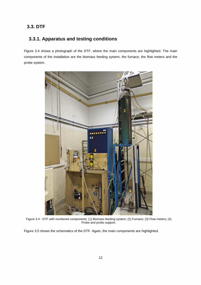
Figure 3.4 shows a photograph of the DTF, where the main components are highlighted. The main
components of the installation are the biomass feeding system, the furnace, the flow meters and the
probe system.
Figure 3.4 - DTF with numbered components: (1) Biomass feeding system; (2) Furnace; (3) Flow meters; (4)
Probe and probe support.
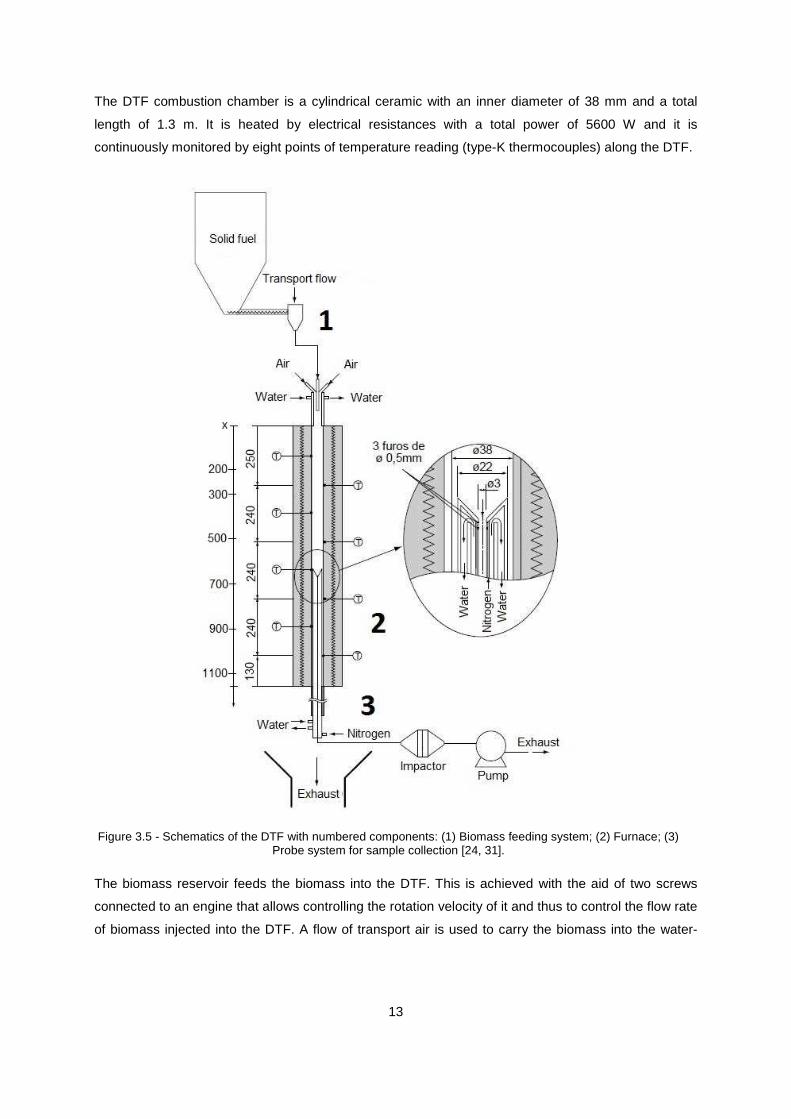
Figure 3.5 shows the schematics of the DTF. Again, the main components are highlighted.
13
The DTF combustion chamber is a cylindrical ceramic with an inner diameter of 38 mm and a total
length of 1.3 m. It is heated by electrical resistances with a total power of 5600 W and it is
continuously monitored by eight points of temperature reading (type-K thermocouples) along the DTF.
Figure 3.5 - Schematics of the DTF with numbered components: (1) Biomass feeding system; (2) Furnace; (3)
Probe system for sample collection [24, 31].
The biomass reservoir feeds the biomass into the DTF. This is achieved with the aid of two screws
connected to an engine that allows controlling the rotation velocity of it and thus to control the flow rate
of biomass injected into the DTF. A flow of transport air is used to carry the biomass into the water-

14
cooled injector placed on top of the DTF. This injector has a second inlet tube where the secondary air
is admitted.
The flow meters allow monitoring both the transport air flow and the secondary air flow to the DTF.
Also, when collecting particles, a flow meter is used to monitor the nitrogen flow rate to the probe
[25, 31] for quenching purposes.
Tests in the DTF were conducted for AF-I (cf. Table 3.1). The tests were conducted for five DTF
temperatures (900, 950, 1000, 1050 and 1100 ºC). The biomass flow rate was 23 g h-1 and the total air
flow rate was 4 L min-1.
3.3.2. Methods
Temperature measurements
The mean gas temperature along the DTF axis is measured with the aid of a thermocouple probe
connected to a data acquisition system, which includes a dedicated computer that uses a software
capable of reading instantaneous temperatures and calculated averages. The thermocouple used is a
type-R with a 76 µm diameter wire platinum and platinum/13% rhodium.
Equation 3.1 expresses an energy balance to the thermocouple bead under steady-state conditions
[24].
�� 0��9:;� <!�9:;� − !> ?@ + / 4 <!�9:;�B − !� ;;B @ = 0 (3.1)
where �� is the Nusselt number, 0 is the conductivity, ��9:;� is the thermocouple bead
diameter, !�9:;� is the temperature of the thermocouple, !> ? is the temperature of the flow gas, / is
the emissivity, 4 is the Stefan-Boltzmann constant and !� ;; is the temperature of the DTF combustion
chamber walls.
Equation 3.1 allows the calculation of the uncertainty of the temperature measurements as it accounts
for the radiation effects from the walls and convection with the gas [24]. It was estimated that there will
be a maximum uncertainty of ± 10% in the measured gas temperature reported for all five DTF
temperatures examined in this study.

15
Burnout measurements
Particle collection for burnout calculations along the DTF was performed isokinetically with the aid of a
water-cooled nitrogen-quenched probe (made of stainless steel with a length of 1.5 m and inner
diameter of 3 mm). Measurements were made along the DTF axis for all DTF temperatures. The
probe is connected to a device with a quartz filter, which is linked to a pump. The nitrogen flow rate
through the probe for quenching purposes was 4.7 L min-1. All procedures follow the European
standards (CEN/TS 14775) [32] and are described with more detail elsewhere [25].
The particle burnout, designated by 2, calculated with the aid of an ash-tracer method, is calculated
as follows:
2 = 1 − 5�561 − 5� (3.2)
where 5� is the ash weight fraction in the input biomass and 56 is the ash weight fraction in the
collected sample.
Uncertainties in particle burnout when using ash as a tracer can be due to ash volatility at high heating
rates and temperatures and ash solubility in water. These uncertainties were found to be negligible for
the conditions used in the present study [31].
16
4. Kinetic Modelling
Smith [33] divided the combustion process of solid fuels into two main stages: (i). devolatilization of
the majority of the biomass volatile matter and production of char; and (ii). homogeneous oxidation of
volatile matter and heterogeneous char oxidation originated during devolatilization. At this point, most
of the volatiles have been burned and there is mainly carbon and inorganic compounds that compose
the ash.
The estimation of the kinetic data is usually performed for each stage, i.e., devolatilization and char
oxidation stages. For each approach, this division can be explained by different reasons. In the TGA,
the stages are more easily identifiable and this division allows to fully understand the differences in
terms of kinetic data from one stage to the other, while maintaining the designated formulation. In the
DTF, the formulation differs and each stage has to be treated individually.
The reaction rate constant, common to the kinetic calculations of either experimental approach, is
described by �:
� = �� FG HIJK (4.1)
where �� is the pre-exponential factor, � is the activation energy, � is the universal gas constant and
! is the temperature. Equation 4.1 is more commonly known as the Arrhenius equation.
This chapter describes the adopted formulation for the kinetic calculations for both experimental
approaches used in this study. For the TGA, kinetic calculations were performed using the CR
method. For the DTF, kinetic calculations were performed with a model-fitting method and a numerical
model. Each section of this chapter, presents the equations, assumptions, input data and calculation
tools. The last section presents the equations for calculating the global kinetic parameters.
4.1. TGA
The TGA formulation adopted in this thesis follows [11], in which a detailed presentation can be found.
The conversion factor or the fraction of biomass that has reacted, is expressed by ,:
, = �L − ��L − �M (4.2)
where �L, �, and �M represent the initial, instantaneous and final stage mass.

17
The reaction rate is generally described by Equations 4.3 and 4.4. In Equation 4.3, the differential
reaction model is given by N(,) and, in Equation 4.4, the integral reaction model is given by �(,):
�,�" = � N(,) (4.3)
�(,) = � " (4.4)
where " is the temporal quantity.
This study considers a first-order reaction model since it is the most common method for describing
the biomass thermal decomposition, as follows [10, 15]:
N(,) = (1 − ,)Q (4.5)
where � is the reaction order.
Substituting Equation 4.1 into Equations 4.3 and 4.4 gives:
�,�" = �� FGHIJK N(,) (4.6)
�(,) = �� FGHIJK " (4.7)
Equation 4.8 can be adopted for non-isothermal experiments, where the non-isothermal reaction rate,
�,/�!, is expressed by:
�,�! = �,�" �"�! (4.8)
where �,/�" is the isothermal reaction rate and �!/�" is the heating rate, also designated by -.
Substituting Equation 4.6 into Equation 4.8 gives:
�,�! = ��- FGHIJK N(,) (4.9)
that expresses the differential form of the non-isothermal reaction rate. Integrating this equation gives:

18
�(,) = ��- S FGHIJKKL �! (4.10)
which expresses the integral form of the non-isothermal reaction rate, also known as the temperature
integral.
Equation 4.10 has to be reformulated into a more general form. To do so, the integration variable has
to be redefined. The new variable can be written as:
& = � �! (4.11)
Substituting Equation 4.11 into Equation 4.10 and rearranging becomes:
�(,) = ��� -! S FG6&T �&M
6 (4.12)
Assuming,
U(&) = S FG6&T �&M
6 (4.13)
The final form of the temperature integral becomes:
�(,) = ��� -� U(&) (4.14)
The Coats-Redfern method takes Equation 4.14 and uses asymptotic series expansion for
approximating U(&) in order to obtain the following expression:
ln �(,) = ln ���-� X1 − 2�!� Z − � �! (4.15)
Because the term TJKHI ≪ 1, it can be neglected, and the final equation can be written as:
ln �(,) = − � �! + ln ���-� (4.16)
where g(α) is given by:
�(,) = −^� (1 − ,)!T , � = 1 (4.17)

19
The plot of ln �(,) vs 1/! generally provides a straight line with a high correlation factor. The apparent
activation energy can be determined from the slope of the line and the pre-exponential factor �� by the
intercept term [34].
In this study, experimental input data include temperature and mass and the calculations were
performed with Matlab, where Equations 4.2, 4.16 and 4.17 were implemented.
4.2. DTF
The equations shared by the two methods used are first presented. The particle weight loss along the
DTF depends on the burnout and on the initial weight. In this sense, in each point, the particle weight
can be calculated in each point by [33]:
� = �L (1 − 2) (4.18)
The rate of devolatilized matter, �$/�", is described by Equation 4.19. The model is based upon a first
order reaction [23, 25]:
�$�" = −�� $ (4.19)
where �� is reaction rate constant for the devolatilization and $ is the volatile content. Equation 4.1
can now be rewritten as:
�� = �� FGHI_JK̀ (4.20)
where �� is the pre-exponential factor and � � is the activation energy for the devolatilization and ! is
temperature of the particle.
The char oxidation, ��/�", is described by Equation 4.21. The model is based upon the outer surface
area of the particles [22, 23, 25]:
���" = −� �� (4.21)
where � is the particle surface area and �� is the reaction rate constant for the char oxidation. The
reaction rate constant for the oxidation �� differs in each method.
20
Equation 4.1 can be rewritten as the reaction rate constant for the oxidation, ��:
�� = �� �ab,? FGHIcJK̀ (4.22)
where �� is the pre-exponential factor for the oxidation, � � is the activation energy for the char
oxidation and �ab,? is the oxygen partial pressure at the particle surface.
Coelho and Costa [4] mentioned how heterogeneous oxidation can be divided into different burning
regimes, depending if the reaction is being controlled chemically (kinetics) or physically (diffusion).
Mitchell et al [35] described each burning regime and pointed out that the physical differences that a
particle suffers. Regime I occurs at low temperatures and is mainly controlled by kinetics (reaction
rates) that limit the mass loss rate. This burning regime implies a process occurring at constant
particle size/diameter and that the apparent density is proportional to the mass loss. Regime II takes
place with increasing temperature. The reaction is now controlled by kinetics and diffusion. During this
regime, particle diameter and apparent densities vary with mass loss. Regime III occurs at higher
temperatures and the reaction rate is mainly controlled by diffusion. The apparent density remains
constant and its diameter varies according to a one-third power law. [4, 8, 35].
Under regime II, the particles’ diameter and density evolution along the combustion process can be
expressed as [33, 35]:
� = �L(1 − 2)d (4.23)
3 = 3L (1 − 2)e (4.24)
where � is the particle diameter, �L is the initial particle diameter, 3 is the particle density and 3L is
the initial particle diameter. For spherical particles, 3, + - = 1. When particles burn under regime I,
the diameter is constant (, = 0) and the density varies proportionally with the mass loss. For particles
burning under regime III the density remains approximately constant (- = 0) and , reaches its
maximum value of 0.33, representing the highest diameter variation. Regime II takes into account the
variation of density and diameter.
21
4.2.1. Model-fitting method
Methodology
This method requires the following simplifications:
• Partial oxygen pressure at particle surface (�ab,g) is considered to be constant and equal to the
partial oxygen pressure of the gas stream throughout the combustion process.
• Particle temperature is assumed to be equal to the gas temperature.
• A single representative diameter (mean diameter) for all particles, constant for the
devolatilization process and varied for the oxidation process.
Calculations with this method fit data with a linear regression for each considered section of the DTF,
as shown in Figure 3.5. The devolatilization process is assumed to fully occur in the upper section,
within section 200 < x < 700 mm, which is further discretized in three different sections:
200 < x < 300, 300 < x < 500, and 500 < x < 700 mm. The devolatilization rate, �$/�", described by
Equation 4.19, can be rewritten considering the experimental burnout as the devolatized matter [25]:
�$�" = −�� (1 − 2) (4.25)
Substituting Equation 4.25 into Equation 4.20 gives [25]:
ln �$�"1 − 2 = − � ��! + ln �� (4.26)
The oxidation process occurs in the rest of the DTF, i.e., 700 < x < 1100 mm of the DTF (cf. Figure
3.5). Substituting equation 4.21 into equation 4.22 gives [24]:
ln ���"−��ab,g= − � ��! + ln �� (4.27)
The kinetic data (� �, � �, ��, ��) can be obtained from Arrhenius plots. In Equation 4.23, parameter ,
can be seen as an apparent diameter variation and is considered to be a fitting parameter.
22
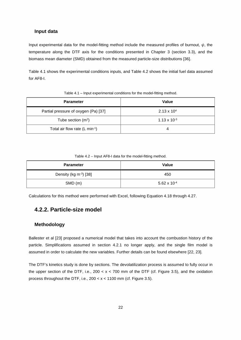
Input data
Input experimental data for the model-fitting method include the measured profiles of burnout, 2, the
temperature along the DTF axis for the conditions presented in Chapter 3 (section 3.3), and the
biomass mean diameter (SMD) obtained from the measured particle-size distributions [36].
Table 4.1 shows the experimental conditions inputs, and Table 4.2 shows the initial fuel data assumed
for AF8-I.
Table 4.1 – Input experimental conditions for the model-fitting method.
Parameter Value
Partial pressure of oxygen (Pa) [37] 2.13 x 10⁴
Tube section (m2) 1.13 x 10⁻³
Total air flow rate (L min-1) 4
Table 4.2 – Input AF8-I data for the model-fitting method.
Parameter Value
Density (kg m-3) [38] 450
SMD (m) 5.62 x 10⁻⁴
Calculations for this method were performed with Excel, following Equation 4.18 through 4.27.
4.2.2. Particle-size model
Methodology
Ballester et al [23] proposed a numerical model that takes into account the combustion history of the
particle. Simplifications assumed in section 4.2.1 no longer apply, and the single film model is
assumed in order to calculate the new variables. Further details can be found elsewhere [22, 23].
The DTF’s kinetics study is done by sections. The devolatilization process is assumed to fully occur in
the upper section of the DTF, i.e., 200 < x < 700 mm of the DTF (cf. Figure 3.5), and the oxidation
process throughout the DTF, i.e., 200 < x < 1100 mm (cf. Figure 3.5).
23
Equations 4.19 and 4.20 describe the devolatilization process for this model. Equation 4.21 accounts
now for the number of biomass particles:
�i � = ���" = −� � �� (4.28)
where �i � is the carbon mass flow and � is the number of biomass particles kg-1 of biomass. Because
particle combustion has two resistance components, diffusion (�����) and kinetics (��) at the surface,
the equivalent electric analogous gives:
���" = −� � 11����� + 1�� �ab,> (4.29)
where ����� is given by:
����� = �ℎ %�� ab )ab� !> (4.30)
and �ℎ is the Sherwood number (�ℎ = 2), %� is the stoichiometric ratio of heterogeneous oxidation, ab
is the mass diffusivity of the oxygen, )ab is the molecular mass of oxygen and !> is the gas stream
temperature.
Carbon at the surface reacts with oxygen producing carbon dioxide [4]:
C + OT → COT (4.31)
The mass balance at the surface of the particle is based on [4]:
���" = �i (ab − �i ab (4.32)
where �i (ab is the carbon dioxide mass flow and �i ab is the oxygen mass flow. Since oxygen is
consumed in the carbon oxidation under stoichiometric proportions, the follow relationship applies:
�i ab = − 1%����" (4.33)
The carbon particle is a porous medium and oxygen diffuses into the particle according to Fick’s law:
�i ab = � m � �ℎ 3> ab(+ab,> − +ab,?) (4.34)

24
where � is the particle diameter, 3> is the gas stream density, and +ab is the mass fraction of the
oxygen for the gas stream or at the surface. Partial oxygen pressure varies throughout the DTF;
substituting the perfect gas equation into Equation 4.34 gives Equation 4.35.
� �ℎ � Lb)9b�!> <�ab,> − �ab,?@ = − 1%�
���" (4.35)
The equation above allows calculating the partial oxygen pressure at the particle surface. Because
oxygen in the gas stream is consumed throughout the length of the DTF due to combustion, in a non-
constant manner, Equation 4.36 describes the partial oxygen evolution with time.
)ab3>�!> � ��ab,>�" = − 1%� �$�" − 1%�
���" (4.36)
where � is the mass flow rate injected into the DTF and %� is the stoichiometric proportion of the
volatile combustion.
Particle temperature differs from gas stream temperature. Equation 4.37 translates the energy balance
equation at the particle surface. Different heat transfer mechanisms are admitted at the particle
surface, such as conduction (�i�9Q� = 0), radiation (�in �) and convection (�i�9Q�) towards the particle
and also heat from devolatilization (��i ) and heterogeneous combustion (�i�):
3 $ � �!�" = �in � + �i�9Q� − �i� + �i� (4.37)
�in � = m �T / 4 (!� ;;B − !B) (4.38)
�i�9Q� = m � �� 0> (!> − !) (4.39)
�i� = 1� �$�" �� (4.40)
25
�i� = 1� ���" �� (4.41)
where $ is the particle volume, � is the specific heat of the biomass, 0> is the thermal conductivity, ��
and �� are the heat of devolatilization and combustion.
Particle-size distribution is taken in account instead of a mean diameter, by grouping different sizes
into classes. Parameters such as proximate analysis, diameters, particle temperature, number of
particles and partial oxygen pressure at the particle surface depend on the size class. The unburnt
fraction, #, considering different classes is:
# = 1 − 2 (4.42)
# = o 5� #�� (4.43)
where 5� is the mass fraction of class 7 and,for this model, # is given as:
# = �$�" + ���" (4.44)
Since calculations are performed considering specific lengths to the point of injection, length,
residence time and velocity variation due to particle class need to be related as follows:
3,� $,� �%,��" = <3,� − 3>@ $,� � − 3 m 1 �,� (%,� − %>) (4.45)
where % is the particle velocity, � is the gravity acceleration, 1 is the viscosity and %> is the gas
stream velocity.
The calculated unburnt fraction is compared with the measured unburnt fraction. The global error
between the experimental and modelled value, ., is calculated by:
. ,p = (#(^)�6 − #(^)q9�) ,p (4.46)
where � and � represent the DTF point and the DTF temperature, respectively. The error for each pair
is estimated as the root mean square of the deviations (Equation 4.47). The pair with the lowest error
is selected as the best representing the kinetic parameters of the biomass fuel tested.

26
. = r 1�q 6�q 6 o o . ,pTst
(4.47)
Input data
Table 4.3 shows the input experimental conditions for the numerical model. Partial pressure of the
oxygen is no longer an input, and additional experimental conditions are included.
Table 4.3 - Input experimental conditions for the numerical model.
Parameter Value
Injection section (m2) 2.55 x 10⁻⁴
Tube section (m2) 1.13 x 10⁻³
Total air flow rate (L min-1) 4
Total work pressure (Pa) 1.01 x 10⁵
Work temperature (ºC) 25
Mass flow rate (g h-1) 23
Table 4.4 shows the input AF8-I data for the numerical model. The mean diameter (SMD) is no longer
an input, and additional fuel data is included. Apart from the data shown in Table 4.4, proximate and
ultimate analysis and particle size distribution (cf. Table 3.1) of AF8-I are also inputs.
Table 4.4 - Input AF8-I data for the numerical model.
Parameter Value
, 0
Density (kg m-3) 450
Specific heat (kJ kg-1 K-1) [39] 2.3
Particle emissivity 1
Table 4.5 shows the input gas properties [40] for the numerical model, which were evaluated for film
temperature [22, 23]. In the model-fitting method, there was no need of assuming any property for the
gas stream, besides the oxygen partial pressure.

27
Table 4.5 - Input gas properties for the numerical model.
Parameter Value
Film temperature (ºC) 1000
Thermal diffusivity (m2 s-1) 2.46 x 10⁻⁴
Viscosity (Pa s) 4.82 x 10⁻⁵
Table 4.6 shows the input heat data for the devolatilization and oxidation [22]. Since particle
temperature is now calculated instead of assuming the measured temperature profile, the heat of
devolatilization and heterogeneous oxidation has to be included.
Table 4.6 - Input heat data for the numerical model.
Parameter Value
Devolatilization heat (J kg-1) 2.07 x 10⁶
Oxidation heat (J kg-1) 9.78 x 10⁶
The kinetic parameters are the inputs and the unknowns to be determined. A pair of activation
energy/pre-exponential factor values is established in order to predict the unburnt fraction for each test
temperature and measured point. When calculating the pair of activation energy/pre-exponential factor
for the devolatilization, the terms related to char oxidation process are set do zero.
The numerical calculations were performed with Mathematica, using Equations 4.19, 4.20 and 4.28
through 4.47.
4.3. Weighted average activation energy
In both model-fitting methods, a stage division of the DTF allow to fit data with high correlation factors.
The objective of this thesis also includes calculating global kinetic parameters, for better
understanding the kinetic data produced by the combustion process as a whole and for comparison
purposes, and so a weighted average process is used to calculate the apparent activation energy.
For the TGA, the weighted average activation energy equation described in [19] is used to calculate
the activation energy of the global combustion process:
� ,� = &�T&�T + &'(u � T + &'(u&�T + &'(u � u (4.48)
28
where &�T is the total volatile matter content, &'(u is the total fixed carbon content, � T is the apparent
activation energy for the second stage and � u is the apparent activation energy for the third stage.
For the DTF, a modified equation based on the previous idea is proposed. The weighted average
activation energy for the global devolatilization process is defined as � >� :
� >� = o &�Q&� � �Q (4.49)
where &�Q represents the fraction of volatile matter in the nth section of the DTF, &� the total volatile
matter and � �Q the apparent activation energy in the nth section of the DTF.
29
5. Results and Discussion
This chapter presents and discusses the results obtained for the TGA and the DTF. The first part of
the chapter is focused on the experimental results. The TGA experiments were performed for the
three biomass samples, whereas the DTF tests were only performed for the AF8-I biomass sample.
The second part of the chapter concentrates on the kinetic data calculated using the models described
in Chapter 4. The third and final part presents comparisons between the kinetic data obtained by
means of the TGA and DTF tests.
5.1. Experimental analysis
5.1.1. TGA
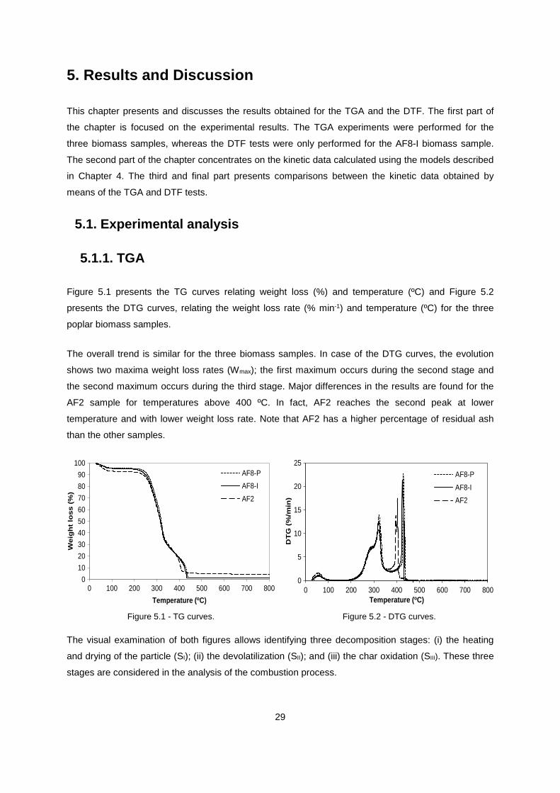
Figure 5.1 presents the TG curves relating weight loss (%) and temperature (ºC) and Figure 5.2
presents the DTG curves, relating the weight loss rate (% min-1) and temperature (ºC) for the three
poplar biomass samples.
The overall trend is similar for the three biomass samples. In case of the DTG curves, the evolution
shows two maxima weight loss rates (Wmax); the first maximum occurs during the second stage and
the second maximum occurs during the third stage. Major differences in the results are found for the
AF2 sample for temperatures above 400 ºC. In fact, AF2 reaches the second peak at lower
temperature and with lower weight loss rate. Note that AF2 has a higher percentage of residual ash
than the other samples.
Figure 5.1 - TG curves. Figure 5.2 - DTG curves.
The visual examination of both figures allows identifying three decomposition stages: (i) the heating
and drying of the particle (SI); (ii) the devolatilization (SII); and (iii) the char oxidation (SIII). These three
stages are considered in the analysis of the combustion process.
Temperature ( oC)
0 100 200 300 400 500 600 700 8000
10
20
30
40
50
60
70
80
90
100
Weig
ht lo
ss (
%)
AF8-P
AF8-I
AF2
0
5
10
15
20
25
DT
G (
%/m
in)
0 100 200 300 400 500 600 700 800Temperature ( oC)
AF8-P
AF8-I
AF2
30
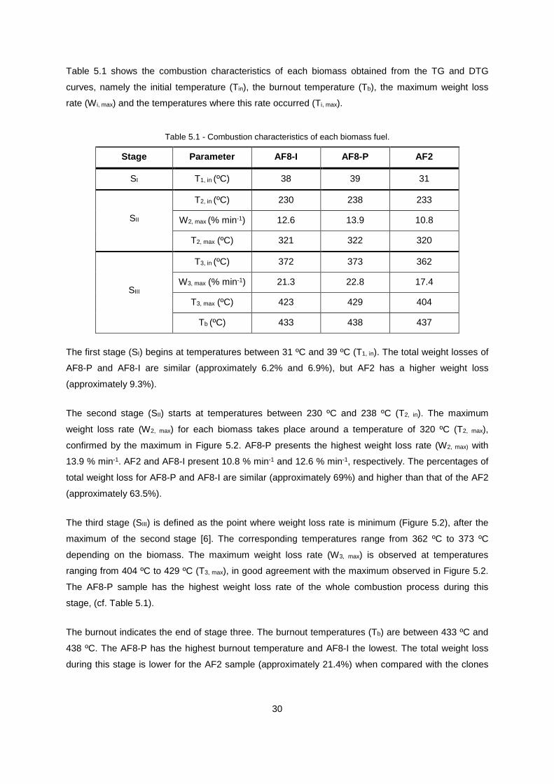
Table 5.1 shows the combustion characteristics of each biomass obtained from the TG and DTG
curves, namely the initial temperature (Tin), the burnout temperature (Tb), the maximum weight loss
rate (W i, max) and the temperatures where this rate occurred (Ti, max).
Table 5.1 - Combustion characteristics of each biomass fuel.
Stage Parameter AF8-I AF8-P AF2
SI T1, in (ºC) 38 39 31
SII
T2, in (ºC) 230 238 233
W2, max (% min-1) 12.6 13.9 10.8
T2, max (ºC) 321 322 320
SIII
T3, in (ºC) 372 373 362
W3, max (% min-1) 21.3 22.8 17.4
T3, max (ºC) 423 429 404
Tb (ºC) 433 438 437
The first stage (SI) begins at temperatures between 31 ºC and 39 ºC (T1, in). The total weight losses of
AF8-P and AF8-I are similar (approximately 6.2% and 6.9%), but AF2 has a higher weight loss
(approximately 9.3%).
The second stage (SII) starts at temperatures between 230 ºC and 238 ºC (T2, in). The maximum
weight loss rate (W2, max) for each biomass takes place around a temperature of 320 ºC (T2, max),
confirmed by the maximum in Figure 5.2. AF8-P presents the highest weight loss rate (W2, max) with
13.9 % min-1. AF2 and AF8-I present 10.8 % min-1 and 12.6 % min-1, respectively. The percentages of
total weight loss for AF8-P and AF8-I are similar (approximately 69%) and higher than that of the AF2
(approximately 63.5%).
The third stage (SIII) is defined as the point where weight loss rate is minimum (Figure 5.2), after the
maximum of the second stage [6]. The corresponding temperatures range from 362 ºC to 373 ºC
depending on the biomass. The maximum weight loss rate (W3, max) is observed at temperatures
ranging from 404 ºC to 429 ºC (T3, max), in good agreement with the maximum observed in Figure 5.2.
The AF8-P sample has the highest weight loss rate of the whole combustion process during this
stage, (cf. Table 5.1).
The burnout indicates the end of stage three. The burnout temperatures (Tb) are between 433 ºC and
438 ºC. The AF8-P has the highest burnout temperature and AF8-I the lowest. The total weight loss
during this stage is lower for the AF2 sample (approximately 21.4%) when compared with the clones

31
AF8 (the total weight loss for the AF8-P is approximately 23.1% and for the AF8-I is approximately
22.4%). The final solid residue (ash) at the end of the third stage is similar for the two clones AF8
(approximately 1.7%) and higher for the AF2 (approximately 5.8%).
The degradation overlap of the structural components creates difficulties in evaluating the influence of
each component alone. In Figure 5.2, hemicellulose is identified by the curve’s shoulder and cellulose
is identified by the curve’s maximum. Lignin slowly decomposes over a wider range of
temperatures [6].
Table 5.2 shows the combustion characteristics of the second stage for woody energy crops samples,
with similar chemical analysis, at 10 ºC min-1 heating rates obtained from literature [9, 12]. Available
parameters such as fuel, temperature interval (Ti, int), maximum weight loss rate (W i, max) and
temperatures where this rate occurred (Ti, max) are indicated for comparative purposes
Table 5.2 - Combustion characteristics of biomass fuels from the literature (second stage).
SII
Reference Fuel T 2, int (ºC) T2, max (ºC) W2, max (% min -1)
[9] Poplar 220 - 400 360 10
Willow 220 - 400 370 10
[12] Poplar 248 - 376 350 -
The initial decomposition temperatures in Table 5.1 are in the range of the initial decomposition
temperatures in Table 5.2 (220 - 248 ºC). The stage ending temperatures in [9] are higher (up to 38 ºC
with a maximum relative error of approximately 10%) than those obtained in the present experiments.
The stage ending temperature in [12] is similar to the stage ending temperature in Table 5.1 (T3, in).
The maximum decomposition temperatures in Table 5.2 (T2, max) are higher (up to 50 ºC) when
compared to the same parameter in Table 5.1, leading to a maximum relative error of approximately
16% when compared to those obtained in the experiments.
The maximum decomposition rates in Table 5.1 (W2, max) are higher than the maximum decomposition
rates in Table 5.2 (up to 3.9 % min-1), leading to a maximum relative error of approximately 28% when
compared to those obtained in the experiments.
Table 5.3 shows the combustion characteristics of the third stage for woody energy crops samples,
with similar chemical analysis, at 10 ºC min-1 heating rates obtained from the literature [9, 12].

32
Table 5.3 - Combustion characteristics of biomass fuels from the literature (third stage)
SIII
Reference Fuel T 3, int (ºC) T3, max (ºC) W3, max (% min -1)
[9] Poplar 340 - 550 457 6.3
Willow 340 - 520 488 6.7
[12] Poplar 391 - 505 450 -
The stage beginning temperatures in Table 5.1 are in the range of the initial decomposition
temperatures in Table 5.3 (340 - 391 ºC). The burnout temperatures in Table 5.3 are higher than the
burnout temperatures in Table 5.1 (up to 117 ºC and maximum relative error of approximately 27%
when comparing the values in Tables 5.1 and 5.3).
The maximum decomposition temperatures in Table 5.3 are higher than those reported in Table 5.1,
with a maximum difference of 84 ºC, leading to a maximum relative error of approximately 17%.
The maximum decomposition rate values in Table 5.1 (W3, max) are higher than the maximum
decomposition rates in Table 5.3 (up to 16.5 % min-1), leading to a maximum relative error of
approximately 72%.
The maximum relative errors reveal more accurate results for the second stage. Differences can be
attributed to a number of factors. In references [9] and [12], initial sample weights are higher than in
this study. Smaller samples allow faster heating rates and shorter analysis times, while larger samples
can lead to combustion at higher temperatures. This may explain the overall differences in the
temperatures. Non-standard methodologies can also alter the analysis. In fact, most studies do not
explicitly indicate how the stage defining temperatures were chosen. As a result of this, the stage
defining temperatures may eventually be different.
According to [8], TG and DTG are empirical tests, with results strongly depending on testing conditions
(heat transfer, heating rate, particle size, sample mass and oxygen concentration) and also on
apparatus and sample characteristics. Solid fuels are not homogeneous and different parameters can
affect the results [12, 13], thus complicating literature comparisons. In order to be comparable, tests
must be conducted under identical operating conditions and in the same testing apparatus [8].
33
5.1.2. DTF
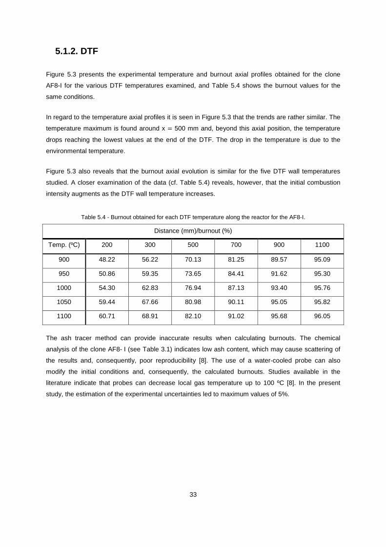
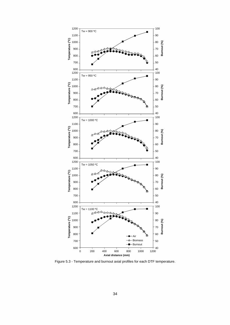
Figure 5.3 presents the experimental temperature and burnout axial profiles obtained for the clone
AF8-I for the various DTF temperatures examined, and Table 5.4 shows the burnout values for the
same conditions.
In regard to the temperature axial profiles it is seen in Figure 5.3 that the trends are rather similar. The
temperature maximum is found around x = 500 mm and, beyond this axial position, the temperature
drops reaching the lowest values at the end of the DTF. The drop in the temperature is due to the
environmental temperature.
Figure 5.3 also reveals that the burnout axial evolution is similar for the five DTF wall temperatures
studied. A closer examination of the data (cf. Table 5.4) reveals, however, that the initial combustion
intensity augments as the DTF wall temperature increases.
Table 5.4 - Burnout obtained for each DTF temperature along the reactor for the AF8-I.
Distance (mm)/burnout (%)
Temp. (ºC) 200 300 500 700 900 1100
900 48.22 56.22 70.13 81.25 89.57 95.09
950 50.86 59.35 73.65 84.41 91.62 95.30
1000 54.30 62.83 76.94 87.13 93.40 95.76
1050 59.44 67.66 80.98 90.11 95.05 95.82
1100 60.71 68.91 82.10 91.02 95.68 96.05
The ash tracer method can provide inaccurate results when calculating burnouts. The chemical
analysis of the clone AF8- I (see Table 3.1) indicates low ash content, which may cause scattering of
the results and, consequently, poor reproducibility [8]. The use of a water-cooled probe can also
modify the initial conditions and, consequently, the calculated burnouts. Studies available in the
literature indicate that probes can decrease local gas temperature up to 100 ºC [8]. In the present
study, the estimation of the experimental uncertainties led to maximum values of 5%.
34
Figure 5.3 - Temperature and burnout axial profiles for each DTF temperature.
Tem
pera
ture
(oC
)T
empe
ratu
re (
oC
)T
empe
ratu
re (
oC
)T
empe
ratu
re (
oC
)T
empe
ratu
re (
oC
)
Bur
nout
(%
)B
urno
ut(%
)B
urno
ut(%
)B
urno
ut (
%)
Bur
nout
(%
)40
50
60
70
80
90
100
40
50
60
70
80
90
100
40
50
60
70
80
90
100
40
50
60
70
80
90
100
40
50
60
70
80
90
100
600
700
800
900
1000
1100
1200
600
700
800
900
1000
1100
1200
600
700
800
900
1000
1100
1200
600
700
800
900
1000
1100
1200
600
700
800
900
1000
1100
1200
0 200 400 600 800 1000 1200
Axial distance (mm)
Axial distance (mm)
Air
Biomass
Burnout
Tw = 900 ºC
Tw = 950 ºC
Tw = 1000 ºC
Tw = 1050 ºC
Tw = 1100 ºC
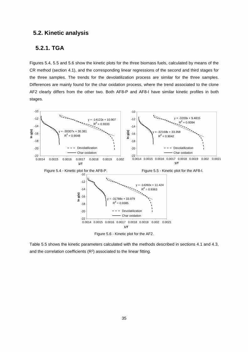
35
5.2. Kinetic analysis
5.2.1. TGA
Figures 5.4, 5.5 and 5.6 show the kinetic plots for the three biomass fuels, calculated by means of the
CR method (section 4.1), and the corresponding linear regressions of the second and third stages for
the three samples. The trends for the devolatilization process are similar for the three samples.
Differences are mainly found for the char oxidation process, where the trend associated to the clone
AF2 clearly differs from the other two. Both AF8-P and AF8-I have similar kinetic profiles in both
stages.
Figure 5.4 - Kinetic plot for the AF8-P. Figure 5.5 - Kinetic plot for the AF8-I.
Figure 5.6 - Kinetic plot for the AF2.
Table 5.5 shows the kinetic parameters calculated with the methods described in sections 4.1 and 4.3,
and the correlation coefficients (R2) associated to the linear fitting.
0.0014 0.0015 0.0016 0.0017 0.0018 0.0019 0.002
1/T
-22
-20
-18
-16
-14
-12
-10
ln g
(α)
y = -30307x + 30.381
R² = 0.9048
y = -14122x + 10.907
R² = 0.9333
Devolatilization
Char oxidation-22
-20
-18
-16
-14
-12
-10
0.0014 0.0015 0.0016 0.0017 0.0018 0.0019 0.002 0.00211/T
ln g
(α)
Devolatilization
Char oxidation
y = -3200x + 9.4815
R² = 0.9394
y = -32168x + 33.358
R² = 0.9042
-22
-20
-18
-16
-14
-12
-10
0.0014 0.0015 0.0016 0.0017 0.0018 0.0019 0.002 0.0021
1/T
ln g
(α)
Devolatilization
Char oxidation
y = -14260x + 11.424
R² = 0.9363
y = -31788x + 33.979
R² = 0.9385

36
Table 5.5 - Kinetic parameters (TGA).
Stage Parameter AF8-I AF8-P AF2
SII
T2, int (ºC) 230 - 374 238 - 375 233 - 363
� (kJ mol-1) 109.74 117.41 118.55
�� (s-1) 1.03 x 10¹¹ 4.62 x 10¹¹ 7.83 x 10¹¹
R2 0.94 0.93 0.93
SIII
T3, int (ºC) 374 - 433 375 - 438 363 - 437
� (kJ mol-1) 267.44 251.97 264.28
�� (s-1) 5.92 x 10²¹ 2.84 x 10²⁰ 1.09 x 10²²
R2 0.90 0.90 0.94
Global � ,� (kJ mol-1) 147.99 150.05 155.36
As shown in Table 5.5, the apparent activation energy in the second stage varies between
109.74 kJ mol-1 and 118.55 kJ mol-1. Both AF8-P and AF2 have similar apparent activation energies,
with values of 117.41 kJ mol-1 and 118.55 kJ mol-1. The apparent activation energy of the AF8-I is the
lowest, with a value of 109.74 kJ mol-1. The apparent pre-exponential factor and the correlation
coefficient for the linear approximations are similar for the three samples.
As seen in Table 5.5, the apparent activation energy in the third stage varies between 251.97 kJ mol-1
and 267.44 kJ mol-1. Both AF2 and AF8-I have similar apparent activation energies, with values of
264.28 kJ mol-1 and 267.28 kJ mol-1. The apparent activation energy of the AF8-P is the lowest, with a
value of 251.97 kJ mol-1. The apparent pre-exponential factor presents different orders of magnitude
for each sample, the highest being that for the AF2. The highest correlation coefficient was obtained
for the AF2.
Table 5.5 reveals that the weighted average activation energy (Global) ranges from 147.99 kJ mol-1
(AF8-I) to 155.36 kJ mol-1 (AF2).
Table 5.6 shows the calculated kinetic parameters of poplar wood under equivalent conditions
available in the literature [12]. Model-free methods were used in these calculations so that only
average values are presented.

37
Table 5.6 - Poplar kinetic parameters reported in the literature (TGA).
Reference Method Heating rate (ºC min -1) vw (kJ mol -1)
[12]
Kissinger
Various
129.20
FWO 141.25
ASTM I 138.10
ASTM II 131.90
The apparent activation energies obtained by [12] are comparable to the weighted average activation
energies obtained in the present study (cf. Table 5.5). The maximum relative error is approximately
equal to 16% and the minimum relative error is approximately equal to 0.4%. Considering that the
values given in [12] were determined with different methods, the relative errors validate the results
included in Table 5.5. It is worth noting that an apparent reaction order of one was assumed in the
present calculations (section 4.1). According to Di Blasi [41], this assumption can influence the
apparent activation energy, yielding higher values. As a result of this, several authors consider to be a
more reliable procedure to compare results with the same kinetic method [12, 15, 18].
When considering literature with calculations performed with the CR method, different apparent
activation energies for the second stage are reported, with values varying from 52 kJ mol-1 [15] to
140 kJ mol-1 [19]. For the third stage, high values for the apparent activation energy with the same
order of magnitude to those included in Table 5.5 can be found in the literature when applying the
present method [18, 34, 42].
The apparent pre-exponential factor values available in the literature show some scattering, varying
from 7.2x10⁶ s-1 [42] to 1.5x10¹⁴ s-1 [19] for the second stage. For the third stage, the apparent pre-
exponential factors reach values as high as 5.7x10²³ s-1 [18]. This means that the apparent pre-
exponential factor is expected to increase as the temperature increases.
Scattering of the results when using the present method have been reported elsewhere [14]. However,
the results in Table 5.5 are in line with the literature and demonstrate how strongly dependent these
data are on the experimental conditions, apparatus and sample characteristics. This problem had
been previously mentioned in section 5.1.1, even in situations when the same method was employed.
Experimental errors can also contribute to the scattering of the apparent kinetic data. In order to be
comparable, tests should be conducted in the same apparatus under similar testing conditions.
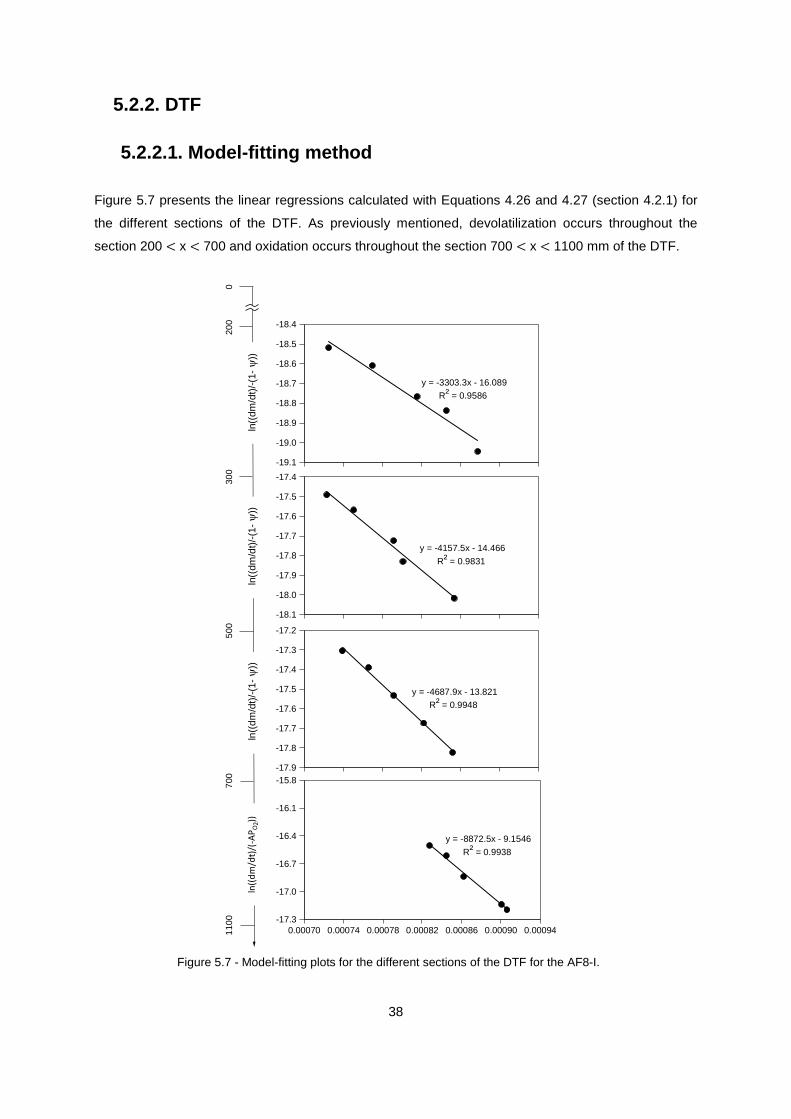
38
5.2.2. DTF
5.2.2.1. Model-fitting method
Figure 5.7 presents the linear regressions calculated with Equations 4.26 and 4.27 (section 4.2.1) for
the different sections of the DTF. As previously mentioned, devolatilization occurs throughout the
section 200 < x < 700 and oxidation occurs throughout the section 700 < x < 1100 mm of the DTF.
Figure 5.7 - Model-fitting plots for the different sections of the DTF for the AF8-I.
-17.3
-17.0
-16.7
-16.4
-16.1
-15.8
-18.1
-18.0
-17.9
-17.8
-17.7
-17.6
-17.5
-17.4
-17.9
-17.8
-17.7
-17.6
-17.5
-17.4
-17.3
-17.2
-19.1
-19.0
-18.9
-18.8
-18.7
-18.6
-18.5
-18.4
0.00070 0.00074 0.00078 0.00082 0.00086 0.00090 0.00094
y = -3303.3x - 16.089
R² = 0.9586
y = -4157.5x - 14.466
R² = 0.9831
y = -4687.9x - 13.821
R² = 0.9948
y = -8872.5x - 9.1546
R² = 0.9938
1100
700
500
300
200
ln((
dm
/dt)
/(-A
PO
2))
0
ln((
dm/d
t)/-
(1-ψ
))ln
((dm
/dt)
/-(1
-ψ
))ln
((dm
/dt)
/-(1
-ψ
))
39
Table 5.7 shows the estimated values of the apparent activation energy, the apparent pre-exponential
factor and the correlation coefficient obtained from linear regressions. The high correlation coefficients
indicate a good agreement between calculated kinetic parameters and experimental data.
Table 5.7 - Kinetic parameters for the model-fitting method for the AF8-I (DTF).
DTF section (mm) vw (kJ mol -1) x (s-1) R2
200 - 300 27.46 9.72 x 10⁻⁸ 0.96
300 - 500 34.57 4.92 x 10⁻⁷ 0.98
500 - 700 38.98 9.39 x 10⁻⁷ 0.99
700 - 1100 73.76 9.98 x 10⁻⁵ 0.99
Throughout the devolatilization zone (200 < x < 700 mm), the apparent activation energy increases
from 27.46 kJ mol-1 (in the first section) to 38.98 kJ mol-1 (in the third section). On the opposite side,
the pre-exponential factor decreases three orders of magnitude. The correlation coefficient is higher
for the second and third sections.
The oxidation zone (700 < x < 1100 mm) has the highest kinetic parameters values. The apparent
activation energy is higher since most of the volatile matter has been released, producing char, and
showing that it is necessary more energy and frequency of collisions for a reaction to occur.
The DTF sections with higher temperatures (Figure 5.3) have lower apparent activation energies. In
fact, when burning biomass the temperature decreases and the apparent activation energy increases
throughout the DTF, leading to the conclusion that the DTF temperature influences the apparent
activation energy.
Table 5.8 presents the overall kinetic parameters. The apparent activation energy for the
devolatilization process was calculated with Equation 4.49 (section 4.3) for the zone 200 < x < 700
mm.
Table 5.8 - Stage kinetic parameters for the model-fitting method for the AF8-I (DTF).
Process vw (kJ mol -1) xy (s-1)
Devolatilization 34.11 -
Oxidation 73.76 9.98 x 10⁻⁵
The apparent activation energies for coal combustion usually varies from 4.18 kJ mol-1 to
188.10 kJ mol-1 [8]. The same reference, i.e., [8], also provides apparent activation energies for the
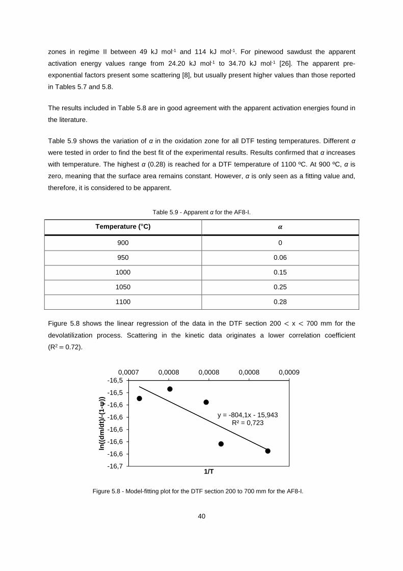
40
zones in regime II between 49 kJ mol-1 and 114 kJ mol-1. For pinewood sawdust the apparent
activation energy values range from 24.20 kJ mol-1 to 34.70 kJ mol-1 [26]. The apparent pre-
exponential factors present some scattering [8], but usually present higher values than those reported
in Tables 5.7 and 5.8.
The results included in Table 5.8 are in good agreement with the apparent activation energies found in
the literature.
Table 5.9 shows the variation of α in the oxidation zone for all DTF testing temperatures. Different α
were tested in order to find the best fit of the experimental results. Results confirmed that α increases
with temperature. The highest α (0.28) is reached for a DTF temperature of 1100 ºC. At 900 ºC, α is
zero, meaning that the surface area remains constant. However, α is only seen as a fitting value and,
therefore, it is considered to be apparent.
Table 5.9 - Apparent α for the AF8-I.
Temperature ( °C) z
900 0
950 0.06
1000 0.15
1050 0.25
1100 0.28
Figure 5.8 shows the linear regression of the data in the DTF section 200 < x < 700 mm for the
devolatilization process. Scattering in the kinetic data originates a lower correlation coefficient
(R2 = 0.72).
Figure 5.8 - Model-fitting plot for the DTF section 200 to 700 mm for the AF8-I.
y = -804,1x - 15,943R² = 0,723
-16,7
-16,6
-16,6
-16,6
-16,6
-16,6
-16,5
-16,50,0007 0,0008 0,0008 0,0008 0,0009
ln((
dm/d
t)/-
(1-ψ
))
1/T
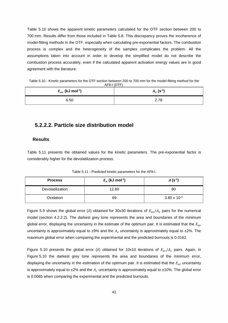
41
Table 5.10 shows the apparent kinetic parameters calculated for the DTF section between 200 to
700 mm. Results differ from those included in Table 5.8. This discrepancy proves the incoherence of
model-fitting methods in the DTF, especially when calculating pre-exponential factors. The combustion
process is complex and the heterogeneity of the samples complicates the problem. All the
assumptions taken into account in order to develop the simplified model do not describe the
combustion process accurately, even if the calculated apparent activation energy values are in good
agreement with the literature.
Table 5.10 - Kinetic parameters for the DTF section between 200 to 700 mm for the model-fitting method for the AF8-I (DTF). vw{ (kJ mol -1) x{ (s-1)
6.50 2.78
5.2.2.2. Particle size distribution model
Results
Table 5.11 presents the obtained values for the kinetic parameters. The pre-exponential factor is
considerably higher for the devolatilization process.
Table 5.11 - Predicted kinetic parameters for the AF8-I.
Process vw (kJ mol -1) x (s-1)
Devolatilization 12.80 90
Oxidation 69 3.80 x 10⁻⁴
Figure 5.9 shows the global error (.) obtained for 30x30 iterations of � �/�� pairs for the numerical
model (section 4.2.2.2). The darkest grey tone represents the area and boundaries of the minimum
global error, displaying the uncertainty in the estimate of the optimum pair. It is estimated that the � �
uncertainty is approximately equal to ±9% and the �� uncertainty is approximately equal to ±2%. The
maximum global error when comparing the experimental and the predicted burnouts is 0.0162.
Figure 5.10 presents the global error (.) obtained for 10x10 iterations of � �/�� pairs. Again, in
Figure 5.10 the darkest grey tone represents the area and boundaries of the minimum error,
displaying the uncertainty in the estimation of the optimum pair. It is estimated that the � � uncertainty
is approximately equal to ±2% and the �� uncertainty is approximately equal to ±10%. The global error
is 0.0065 when comparing the experimental and the predicted burnouts.
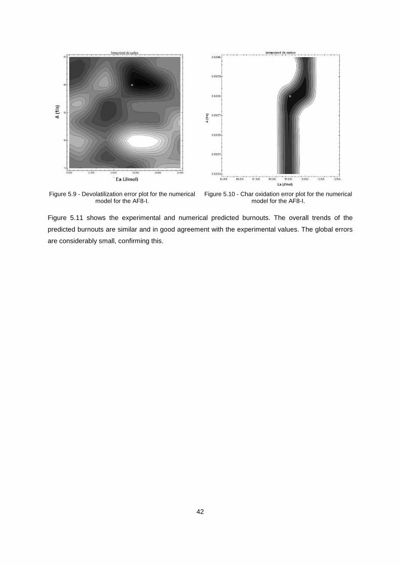
42
Figure 5.9 - Devolatilization error plot for the numerical
model for the AF8-I. Figure 5.10 - Char oxidation error plot for the numerical
model for the AF8-I.
Figure 5.11 shows the experimental and numerical predicted burnouts. The overall trends of the
predicted burnouts are similar and in good agreement with the experimental values. The global errors
are considerably small, confirming this.
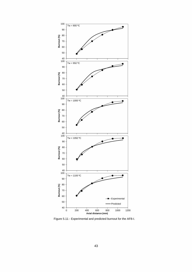
43
Figure 5.11 - Experimental and predicted burnout for the AF8-I.
40
50
60
70
80
90
100
Bur
nou
t(%
)
40
50
60
70
80
90
100
Bur
nou
t(%
)
40
50
60
70
80
90
100
Bur
nou
t(%
)
40
50
60
70
80
90
100
Bur
nou
t(%
)
40
50
60
70
80
90
100B
urno
ut(
%)
0 200 400 600 800 1000 1200Axial distance (mm)
Tw = 900 ºC
Tw = 950 ºC
Tw = 1000 ºC
Tw = 1050 ºC
Tw = 1100 ºC
Experimental
Predicted

44
The burnout prediction of the char oxidation process strongly relies on the pair � �/��. Since these
values were calculated for the DTF section 200 < x < 700 mm as an approximation, predicted values
might not be completely reliable. A more accurate method of calculating � �/�� is needed.
Literature previously mentioned in section 5.2.2.1 confirms these results. In reference [8], the apparent
activation energies for coal vary between 4.18 kJ mol-1 and 188.1 kJ mol-1, but in [26] the results
reported for the apparent activation energy associated to the devolatilization process are higher.
In what concerns the apparent kinetic parameters, values are in good agreement with the
literature [22]. The apparent pre-exponential factors are expected to be higher than the apparent pre-
exponential factor determined for the oxidation process [8].
Data scattering due to experimental differences explained in section 5.2.2.1 also apply to this section.
In conclusion, the results obtained with this model are consistent with the literature [8, 22].
Sensitivity analysis
Since the experiments were not carried out under pyrolytic conditions and there is no literature on the
devolatization kinetic parameters in a drop tube furnace for poplar, it is important to perform a
sensitivity analysis.
The results in section 5.2.2.2 consider burning in regime I (α = 0) in order to optimize the results.
Since the analysis in section 5.2.2.1 considers burning in regime II within a certain section of the DTF,
a sensitivity analysis had to be done for α. However, the results obtained are similar so they are not
addressed here.
Two scenarios are considered for the estimation of the kinetic parameters for the oxidation process. In
the first scenario, calculations were performed considering the weighted average kinetic parameters1
estimated for the model-fitting method as inputs: � � = 34.1 kJ mol-1 and �� = 5.7 x 10⁻⁷ s-1 (section
5.2.2.1). In the second scenario, calculations were performed considering the devolatilization kinetic
parameters when model fitting is applied to the DTF section 200 < x < 700 mm: � � = 6.5 kJ mol-1
and �� = 2.78 s-1 (section 5.2.2.1).
Figures 5.12 and 5.13 present the global error (.) for 10x10 iterations of � �/�� pairs for the two
above mentioned scenarios. In the first scenario, the uncertainty of the pair is approximately
± 2%/± 20% and, in the second scenario, the uncertainty of the pair is approximately ± 0.8%/± 8%
1 In case of the pre-exponential factor, this was only done for case study purposes. Ideally, a model-fitting method for calculating the pre-exponential factor should have been applied [18].

45
Figure 5.12 - Oxidation error plot for the first scenario
of the sensitivity analysis for the AF8-I. Figure 5.13 - Oxidation error plot for the second scenario of the sensitivity analysis for the AF8-I.
Table 5.12 summarizes the calculated global error (.), apparent activation energy and pre-exponential
factor for both scenarios. The second scenario produces a lower global error and apparent activation
energy but a higher pre-exponential factor than that of the first scenario.
Table 5.12 - Kinetic data obtained for both scenarios.
Scenario | vw} (kJ mol -1) x} (1 s-1)
First 0.0144 82.50 3.70 x 10⁴
Second 0.0132 64 5.50 x 10³
Comparing with the values calculated in section 5.2.2.2, the global error for both scenarios is higher
than the global error previously calculated (. = 0.0065). Previously calculated apparent activation
energy (� � = 69 kJ mol-1) is closer to the apparent activation energy value calculated in the first
scenario. The previously calculated pre-exponential factor (�� = 3.6 x 10⁻⁴ s-1) is lower than the pre-
exponential factor calculated for both scenarios and included in Table 5.12. For higher � �/�� pairs
(first scenario), a higher � �/�� pair is to be expected while for lower � �/�� pairs (second scenario), a
lower � �/�� pair is to be expected.
Figure 5.14 shows the experimental and numerical predicted burnout for the first scenario and Figure
5.15 shows the experimental and predicted burnout for the second scenario.

46
Figure 5.14 - Experimental and predicted burnout for the AF8-I in the first scenario.
Bur
nou
t(%
)B
urno
ut
(%)
Bur
nou
t(%
)B
urno
ut
(%)
Bur
nou
t(%
)40
50
60
70
80
90
100
40
50
60
70
80
90
100
40
50
60
70
80
90
100
40
50
60
70
80
90
100
40
50
60
70
80
90
100
0 200 400 600 800 1000 1200Axial distance (mm)
Axial distance (mm)Tw = 950 ºC
Tw = 1000 ºC
Tw = 1050 ºC
Tw = 1100 ºC
Tw = 900 ºC
Experimental
Predicted

47
Figure 5.15 - Experimental and predicted burnout for the AF8-I in the second scenario.
The previous figure shows how the devolatilization kinetic data can impact the kinetic and burnout
data for the oxidation process. Comparing Figure 5.11 with Figures 5.14 and 5.15 it is possible to
40
50
60
70
80
90
100
Bur
nou
t(%
)
40
50
60
70
80
90
100B
urno
ut
(%)
40
50
60
70
80
90
100
Bur
nou
t(%
)
40
50
60
70
80
90
100
Bur
nou
t(%
)
40
50
60
70
80
90
100
Bur
nou
t(%
)
0 200 400 600 800 1000 1200Axial distance (mm)
Experimental
Predicted
Tw = 900 ºC
Tw = 950 ºC
Tw = 1000 ºC
Tw = 1050 ºC
Tw = 1100 ºC

48
observe that, in both scenarios, the predicted burnout curves are no longer in such a good agreement,
as they were previously, thereby increasing the global error.
5.2.2.3. Comparison between methods
Table 5.13 shows the apparent kinetic parameters for the devolatilization and char oxidation stages
estimated by the two previously considered methods for the same sections of the DTF (Tables 5.8 and
5.11). The devolatilization and oxidation apparent activation energies are higher when calculated by
the model-fitting method.
Concerning the apparent activation energies, comparison of the data included in Table 5.13 gives a
relative error of 62% for the devolatilization process and a relative error of 7% for the oxidation against
the values obtained with the model-fitting method. The apparent pre-exponential factor calculated by
both methods originates very distinct values.
Table 5.13 - Kinetic data comparison for the AF8-I (DTF).
Method vw{ (kJ mol -1) x{ (s-1) vw} (kJ mol -1) x} (s-1)
Model-fitting 34.11 - 73.77 1.00 x 10⁻⁴
Numerical 12.80 90 69 3.80 x 10⁻⁴
The results show that the model-fitting method can be used to obtain a fast estimation for the apparent
activation energies. The main drawback of numerical methods is the computation time. However, the
assumptions taken into account in the model-fitting method (section 4.2.1) do not describe the
combustion process accurately, even if calculating satisfactory apparent activation energy values and
in good agreement with the literature. The combustion process is not linear and should not be treated
as so. The assumptions in the particle-size model (section 4.2.2) replicate more accurately the
combustion process for a solid particle. For these reasons, the apparent kinetic data calculated with
the particle-distribution model is considered to be more accurate.
5.2.3. TGA versus DTF
Both experimental techniques reveal the presence of unburnt material. The TGA of AF8-I (section
5.1.1) indicated a final weight of approximately 1.7%, kept constant from a temperature of 430 ºC to
the end of the combustion process while the DTF (section 5.1.2) indicated unburnt samples with a final
weight up to 4% (from the experimental data). This leads to the conclusion that the heating rate and
analysis period influences the release of the volatile and/or inorganic matter.

49
Table 5.14 summarizes the kinetic data calculated for slow and fast combustion using the methods
previously described in Chapter 4. Apparent kinetic parameters obtained under slow and fast
combustion differ. As seen, TGA apparent kinetic data displayed in Table 5.14 is higher than the
calculated values for either DTF kinetic models included in the same table, leading to the conclusion
that the heating rate also influences the kinetic data.
Table 5.14 - Kinetic data comparison under slow and fast combustion for the AF8-I.
Method vw{ (kJ mol -1) x{ (s-1) vw} (kJ mol -1) x} (s-1)
CR 109.74 1.03 x 10¹¹ 267.44 5.92 x 10²¹
Model-fitting 34.11 - 73.77 1.00 x 10⁻⁴
Numerical 12.80 90 69 3.80 x 10⁻⁴
As previously discussed, the estimated apparent kinetic parameters present some differences with
those available in the literature. Each experimental approach present advantages when compared to
the other. On one hand, the TGA is a versatile, fast and easy way of simulating combustion in regime
I. Also, available kinetic data for the TGA is relatively easy to find because this method is the most
used. On the other hand, the DTF is known to better describe realistic boiler combustion conditions.
This experimental reactor is capable of simulating realistic surrounding combustion atmosphere, while
working at high temperatures and heating rates [27, 43]. Since experimental conditions strongly affect
the results, kinetic data obtained with the DTF are closer to that prevailing in industrial boilers.
Hesitations on the kinetic data calculated with the TGA have been addressed for different reasons [8]:
(i). unrealistic operating temperatures, (ii). slow heating rates, influencing the devolatilization and char
formation, (iii). difficulty in identifying the combustion stages with accuracy, and (iv). measured
temperatures are not necessarily identical to the sample temperature.

50
6. Conclusions and Future Work
This work focused on evaluating the burning capabilities of three short rotation coppice poplar wood
samples and calculating the kinetic parameters under slow and fast combustion conditions, while
understanding what can influence the obtained data. TGA was performed for the three samples at a
heating rate of 10 ºC min-1, and DTF experiments were performed at five temperatures (900, 950,
1000, 1050 and 1100 ºC) for one of the samples.
TG/DTG curves indicate the existence of three main combustion stages: drying and heating of the
particle, devolatilization and char oxidation. Calculated kinetic data showed good agreement with the
values reported in the literature.
DTF experiments showed that overall particle burnouts are similar at the exit of the DTF regardless of
the all DTF wall temperature. Kinetic data obtained through two distinct methods are in line with the
values reported in the literature.
Comparisons between the TGA and DTF data showed that the heating rate can influence significantly
the kinetic data: TGA experiments provide higher kinetic values than to those obtained from the DTF
experiments. The kinetic data obtained with the DTF is, however, more representative of industrial
combustion conditions.
In future, TGA tests conducted at different heating rates could be interesting to explore model-free
kinetic modelling and compare with model-fitting methodology. Also, a comparative study on air/inert
atmosphere can be useful.
Because short rotation coppice poplar has so much potential as an alternative fuel, it would be
interesting in future to evaluate its potential to be used in co-firing processes with coal in power
stations, particularly in regard to its environmental impact.
51
7. References
[1] European Commission. http://ec.europa.eu/.
[2] Afas, N.A., Marron, N., Dongen, S.V., Laureysens, I., Caulemans, R. Dynamics of biomass
production in a poplar coppice culture over three rotations (11 years). Forest Ecology and
Management, 255:1883-1891, 2008.
[3] McKendry, P. Energy production from biomass (Part 2): Conversion Technologies. ScienceDirect,
83:47-54, 2012.
[4] Coelho, P., Costa, M. Combustão. Orion, 2007.
[5] Ferreiro, A.I.M., Pyrolysis of pine bark, wheat straw and rice Husk: thermogravimetric analysis and
kinetic study. MSc Thesis, Instituto Superior Tecnico, Lisboa, 2015.
[6] Ferreira, P.T.F.A. Combustion of alternative biomass fuels in a domestic boiler and in a large-scale
furnace. PhD Thesis, University of Minho, 2016.
[7] White, J.E., Catallo, W.J., Legendre, B.L. Biomass pyrolysis kinetics: A comparative critical review
with relevant agricultural residue case studies. Journal of Analytical and Applied Pyrolysis, 91:1-33,
2011.
[8] Carpenter, A.M., Skorupska, N.M. Coal combustion – analysis and testing. IEA Coal Research,
1993.
[9] Karampinis, E., Vamvuka, D., Sfakiotakis, S., Grammelis, P., Itskos, G., Kakaras, E. Comparative
study of combustion properties of five energy crops and Greek lignite. Energy & Fuels, 26:869-878,
2012.
[10] Slopiecka, K., Bartocci, P., Fantozzi, F. Thermogravimetric analysis and kinetic study of poplar
wood pyrolysis. Applied Energy, 97:491-497, 2012.
[11] Khawam, A. Application of solid-state kinetics to desolvation reactions. PhD Thesis, University of
Iowa, 2007.
[12] Kok, M., Ozgur, E. Thermal analysis and kinetics of biomass samples. Fuel Processing
Technology, 106:739-743, 2013.

52
[13] Islam, M., Auta, M., Kabir, G., Hameed, B.H. A thermogravimetric analysis of the combustion
kinetics of karanja (Pongamia pinnata) fruit hulls char. Bioresource Technology, 200:335-341, 2016.
[14] Ebrahimi-Kahrizsangi, R., Abbasi, M.H. Evaluation of reliability of Coats-Redfern method for
kinetic analysis of non-isothermal TGA. Transactions of Nonferrous Metals Society of China, 18:217-
221, 2008.
[15] Yorulmaz, S.Y., Atimtay, A. Investigation of combustion kinetics of five waste woods samples with
thermogravimetric analysis. Environmental Earth Sciences, 90:511-520, 2011.
[16] Jeguirim, M., Dorge, S., Trouvé, G. Thermogravimetric analysis and emission characteristics of
two energy crops in air atmosphere. Bioresource Technology, 101:788-793, 2010
[17] Karaosmanoglu, F., Çift, B., Isigigur-Ergudenler, A. Determination of reaction kinetics of straw and
stalk of rapeseed using thermogravimetric analysis. Energy Sources, 23:767-774, 2001.
[18] López-González, D., Fernandez-Lopez, M., Valverde, J.L., Sanchez-Silva, L. Thermogravimetric-
mass spectrometric analysis on combustion of lignocellulosic biomass. Bioresource Technology,
143:562-574, 2013.
[19] Fang, X., Jia, L., Yin, L. A weighted average global process model based on two-stage kinetic
scheme for biomass combustion. Biomass and Bioenergy, 48:43-50, 2013.
[20] López-González, D., Avalos-Ramirez, A., Giroir-Fendler, A., Godbout, S., Fernandez-Lopez, M.,
Sanchez-Silva, L., Valverde, J.L. Combustion kinetic study of woody and herbaceous crops by thermal
analysis coupled to mass spectrometry. Energy, 90:1626-1635, 2015.
[21] Farrow. T.S., Sun, C., Snape, C.E. Impact of CO2 on biomass pyrolysis, nitrogen partitioning, and
char combustion in a drop tube furnace. Journal of Analytical and Applied Pyrolysis, 113:323-331,
2015.
[22] Jiménez, S., Remacha, P., Ballesteros, J.C., Giménez, A., Ballester, J. Kinetics of devolatilization
and oxidation of a pulverized biomass in an entrained flow reactor under realistic combustion
conditions. Combustion and Flame, 152:588-603, 2008.
[23] Ballester, J., Jiménez, S. Kinetic parameters for the oxidation of pulverized coal as measured
from drop tube tests. Combustion and Flame, 142:210-222, 2005.

53
[24] Wang, G., Silva, R.B., Azevedo, J.L.T., Martins-Dias, S., Costa, M. Evaluation of the combustion
behaviour and ash characteristics of biomass waste derived fuels, pine and coal in a drop tube
furnace. Fuel, 117:809-824, 2014.
[25] Costa, F., Wang, G., Costa, M. Combustion kinetics and particle fragmentation of raw and torrified
pine shells and olive stones in a drop tube furnace. Proceedings of the Combustion Institute, 35:3591-
3599, 2014.
[26] Authier, O., Thunin, E., Plion, P., Porcheron, L. Global kinetic modelling of coal devolatilization in
a thermogravimetric balance and drop-tube furnace. Energy & Fuels, 29:1461-1468, 2015.
[27] Zellagui, S., Schonnenbeck, C., Zouaoui-Mahzoul, N., Leyssens, G., Authier, O., Thunin, E.,
Porcheron, L., Brilhac, J.-F. Pyrolysis of coal and woody biomass under N2 and CO2 atmospheres
using a drop tube furnace – experimental study and kinetic modelling. Fuel Processing Technology,
148:99-109, 2016.
[28] SHIMADZU. www.shimadzu.com.
[29] College of Chemistry and Molecular Engineering. www.chem.pku.edu.cn.
[30] Yuzbasi, N.S., Selçuk, N. Air and oxy-fuel combustion characteristics of biomass/lignite blends in
TGA-FTIR. Fuel Processing Technology, 92:1101-1108, 2011.
[31] Wang, G., Zander, R., Costa, M. Oxy-fuel combustion characteristics of pulverized-coal in a drop
tube furnace. Fuel, 115:452-460, 2014.
[32] BSI. www.bsigroup.com.
[33] Smith, I. The combustion rates of coal chars: A review. Proceedings of the Combustion Institute,
19:1045-1065, 1982.
[34] Ferreira, A., Soares Dias, A., Silva, C. M., Costa, M. Evaluation of thermochemical properties of
raw and extracted microalgae. Energy, 92:365-372, 2015.
[35] Mitchell, R.E., Ma, L., Kim, B. On the burning behaviour of pulverized coal chars. Combustion and
Flame, 151:426-436, 2007.
[36] HORIBA. www.horiba.com.

54
[37] Foulkes, F.R. Physical Chemistry for Engineering and Applied Sciences. Taylor & Francis Group,
LL, 2013.
[38] Workshop. https://cedarstripkayak.wordpress.com/.
[39] WOODPRODUCTS. http://www.woodproducts.fi
[40] Incropera, F.P., DeWitt, D.P., Bergman, T.L., Lavine, A.S. Fundamentals of Heat and Mass
Transfer. John Wiley & Sons, 2006.
[41] Di Blasi, C. Modelling chemical and physical processes of wood and biomass pyrolysis. Progress
in Energy and Combustion Science, 34:47-90, 2008.
[42] Shen, D.K., Gu, S., Luo, K.H., Bridgwater, A.V., Fang, M.X. Kinetic study on thermal
decomposition of woods in oxidative environment. Fuel, 88:1024-1030, 2009.
[43] Pottmaier, D., Costa, M., Farrow, T., Oliveira, A.A.M., Alarcon, O., Snape, C. Comparison of rice
husk and wheat straw: From slow and fast pyrolysis to char combustion. Energy & Fuels, 27:7115-
7125, 2013.


