
2015s-50
Labor Market Policies and Self-Employment
Transitions of Older Workers
Dimitris Christelis, Raquel Fonseca
Série Scientifique/Scientific Series

Montréal
Novembre/November 2015
© 2015 Dimitris Christelis, Raquel Fonseca. Tous droits réservés. All rights reserved. Reproduction partielle
permise avec citation du document source, incluant la notice ©.
Short sections may be quoted without explicit permission, if full credit, including © notice, is given to the source.
Série Scientifique
Scientific Series
2015s-50
Labor Market Policies and Self-Employment
Transitions of Older Workers
Dimitris Christelis, Raquel Fonseca

CIRANO
Le CIRANO est un organisme sans but lucratif constitué en vertu de la Loi des compagnies du Québec. Le financement de son
infrastructure et de ses activités de recherche provient des cotisations de ses organisations-membres, d’une subvention
d’infrastructure du Ministère de l'Économie, de l'Innovation et des Exportations, de même que des subventions et mandats
obtenus par ses équipes de recherche.
CIRANO is a private non-profit organization incorporated under the Québec Companies Act. Its infrastructure and research
activities are funded through fees paid by member organizations, an infrastructure grant from the Ministère de l' l'Économie,
de l'Innovation et des Exportations, and grants and research mandates obtained by its research teams.
Les partenaires du CIRANO
Partenaires corporatifs
Autorité des marchés financiers
Banque de développement du Canada
Banque du Canada
Banque Laurentienne du Canada
Banque Nationale du Canada
Bell Canada
BMO Groupe financier
Caisse de dépôt et placement du Québec
Fédération des caisses Desjardins du Québec
Financière Sun Life, Québec
Gaz Métro
Hydro-Québec
Industrie Canada
Intact
Investissements PSP
Ministère de l'Économie, de l'Innovation et des Exportations
Ministère des Finances du Québec
Power Corporation du Canada
Rio Tinto
Ville de Montréal
Partenaires universitaires
École Polytechnique de Montréal
École de technologie supérieure (ÉTS)
HEC Montréal
Institut national de la recherche scientifique (INRS)
McGill University
Université Concordia
Université de Montréal
Université de Sherbrooke
Université du Québec
Université du Québec à Montréal
Université Laval
Le CIRANO collabore avec de nombreux centres et chaires de recherche universitaires dont on peut consulter la liste sur son
site web.
ISSN 2292-0838 (en ligne)
Les cahiers de la série scientifique (CS) visent à rendre accessibles des résultats de recherche effectuée au CIRANO afin
de susciter échanges et commentaires. Ces cahiers sont écrits dans le style des publications scientifiques. Les idées et les
opinions émises sont sous l’unique responsabilité des auteurs et ne représentent pas nécessairement les positions du
CIRANO ou de ses partenaires.
This paper presents research carried out at CIRANO and aims at encouraging discussion and comment. The observations
and viewpoints expressed are the sole responsibility of the authors. They do not necessarily represent positions of CIRANO
or its partners.
Labor Market Policies and Self-Employment Transitions
of Older Workers*
Dimitris Christelis†, Raquel Fonseca‡
Résumé/abstract
We study transitions in and out of self-employment of older individuals using internationally comparable
survey data from 13 OECD countries. We compute selfemployment transitions as conditional
probabilities arising from a discrete choice panel data model. We examine the influence on self-
employment transitions of labor market policies and institutional factors (employment protection
legislation, spending on employment and early retirement incentives, unemployment benefits, strength
of the rule of law), as well as individual characteristics like physical and mental health. Selfemployment
is strongly affected by government policies: larger expenditures on employment incentives impact it
positively, while the opposite is true for expenditures on early retirement and unemployment benefits.
Mots clés/keywords : self-employment, transitions, ageing, labor policies, panel
data
Codes JEL/JEL Codes : J21, J24, C4
* We thank Arthur van Soest and Simon Parker for their useful comments. Christelis acknowledges financial
support from the European Union and the Greek Ministry of Education under Program Thales, grant MIC
380266. Fonsceca aknowledges support from the National Institute on Aging, grant P01 AG022481 and SSHRC
Insight Grants. This research is also part of the program of the Industrial Alliance Research Chair on the
Economics of Demographic Change. † University of Naples Federico II, CSEF, CFS and CEPAR ‡ Université du Québec à Montréal, CIRANO and RAND
2
1. Introduction
The prevalence of self-employment varies widely across countries, e.g. it is quite
higher in Southern Europe than in Northern Europe. Furthermore, self-employment
becomes more common with age, partly because it provides older workers with
opportunities not found in traditional salary jobs, such as flexibility in working hours.
This is particularly important because older workers may have different preferences for
leisure than younger ones, as well as for a more gradual retirement path. Self-
employment may also facilitate such a retirement path, (see Quinn, 1980, and Fuchs,
1982), which can be of interest to policy makers who aim to boost working at older ages.
Hence, the effect of labor market policies on self-employment in older age merits
further investigation. However, while there is a large literature that compares different
self-employment rates across countries2, there are few studies that focus on transitions in
and out of self-employment of older workers, and on how labor market policies affect
such transitions. Zissimopoulos et al. (2009) examine the role of incentives related to
private pensions and public health insurance on the retirement patterns of wage earners
and the self-employed in the US and the UK, using data from the Health and Retirment
Study (HRS) and the English Longitudinal Survey of Ageing (ELSA). Furthermore,
Zissimopoulos and Karoly (2007) study the role of wealth and health in transitions
related to self-employment in the US using the HRS.
Cross-country comparisons of self-employment patterns of older workers are also
rare. One exception is Hochguertel (2005), who examines the role of institutional and 2 See e.g. Blanchflower and Oswald (1998), Blanchflower (2000), Parker (2004), and Hyytinen and Rouvinen (2007).
3
demographic factors on the prevalence of self-employment in 11 European countries
using data from the Survey of Health, Ageing and Retirement in Europe (SHARE). In
addition, Fonseca et al. (2007), using data from HRS, ELSA and SHARE study the effect
of liquidity constraints on entrepreneurship. Carrasco and Ejrnæs (2003) examine
institutional factors such as the generosity of the unemployment benefit system and child
care policies in two countries, namely Spain and Denmark, which have a high and a low
prevalence of self-employment, respectively. Carrasco and Ejrnæs estimate transitions
into self-employment in the population using logit models for both women and men,
conditional on their previous labor market status. They find that differences in the
generority of unemployment benefits are indeed associated with differences in labor
market dynamics between the two countries. Most of the available studies on the self-
employed, however, are country-specific.3
Our contribution in this paper is to analyze the effect of labor market policies on
transitions in and out of self-employment of older workers in 13 OECD countries, using
data from SHARE, HRS and ELSA. Data on both labor market policies at the country
level and on self-employment policies at the individual level are harmonized across
countries, and hence meaningful cross-country comparisons can be made. The labor
market policies that we examine include employment protection legislation, early
retirement and employment incentives, unemployment benefits and the rule of law (see
also Torrini, 2005).
In contrast to previous work on self-employment transitions, we use an empirical
3 See, for example, Bruce et al. (2000), who find that government incentives in the last decades have affected the occupational choice of older workers in the US. The relationship between social security generosity and self-employment transitions is also examined in Carrasco (1999) for Spain, and Been and Knoef (2012) for the Netherlands, among others. Other examples include Quinn (1980), Fuchs (1982), Bound et al. (1999), Bruce et al. (2000), Giandrea et al. (2008) for the US economy

4
methodology that allows us to compute transitions in and out of self-employment in older
age as conditional probabilities arising naturally from a discrete choice panel data model
that takes into account selectivity in the sample of older workers, as well as the
autocorrelation of all time-varying unobservable factors present in the estimating
equations. Hence, using this model we are able to study how self-employment transitions
are affected by the aforementioned country-level institutional factors as well as by
individual-level characteristics.
We find that self-employment transitions are strongly associated labor market
policies: increased expenditures on employment incentives affect make it more likely that
older age individuals will become self-employed, while the opposite is true for
expenditures on early retirement and unemployment benefits. In addition, employment
protection legislation favors self-employment, as it makes it more difficult to find a job as
a salaried worker. We also find that self-employment is negatively associated with the
rule of law, probably due to the fact that the self-employed can benefit from weak law
enforcement more than salaried workers. Finally, we find that entering and remaining
into self-employment is facilitated by good physical and mental health, and hindered
when one is female or has grandchildren.
The structure of the paper is as follows: In Section 2 describes our data, while
Section 3 discusses the estimation methodology. We present our empirical results in
Section 4, while Section 5 concludes.
2. Data and empirical overview
2.1. Data

5
The empirical analysis in this study is based on three datasets: the HRS for the U.S.,
ELSA for England and SHARE for 11 European countries.4 These surveys consist of
representative samples of the population aged fifty and above in all countries. The data
used in this study are taken from waves 7 and 8 of the HRS, waves 2 and 3 of the ELSA,
and waves 1 and 2 of the SHARE.5 The first wave in each survey was conducted in 2004-
2005 while the second in 2006-2007. Importantly, these three surveys have been to a
large extent harmonized with respect to their questionnaire. As a result, they provide
harmonized data on our variables of interest, namely those on employment, and on
various demographics and economic characteristics.
In addition, we also use variables related to labor market policies such as
employment protection laws, and labor incentives that are taken from OECD and World
Bank datasets. We describe all the variables in more detail below.
In our analysis we restrict our sample to those aged 75 or less, as individuals older
than 75 are very unlikely to be working in any capacity or to transition into self-
employment. The basic statistics of the sample we use in the estimation are reported in
Table 1, which summarizes demographic variables (education, age, gender, marital
status, number of children and grandchildren) and physical and mental health variables
(self-reported health, depression and the score on an immediate recall test) that have been
found in existing literature to affect self-employment transitions. We choose to use in our
4 We include the countries that are present in the first two waves of SHARE, namely Sweden, Denmark, Germany, the Netherlands, Belgium, France, Switzerland, Austria, Italy, Spain, and Greece. There is one additional comparable SHARE wave that took place after 2007 (namely the fourth one of 2010-11), as well as HRS and ELSA waves that took place in 2008 and 2010. However, the recent financial crisis may affect our analysis by inducing differential occupational transitions and increases in unemployment rates across countries. Incorporating these effects is, however, potentially informative on its own, and thus we leave it for further research. 5 The third SHARE wave, also known as SHARELIFE, is a retrospective survey that has a very different questionnaire than the previous two waves. Hence, we cannot use SHARELIFE in our analysis.
6
specifications only variables that are less likely to be endogenous to the self-employment
decision.
We note that about 45% of individuals in our sample are working. There are large
differences, however, in inactivity rates across countries, as can be seen in Table 2, which
also shows that self-employment rates differ markedly also by gender. In the
Mediterranean countries, Austria and Belgium two thirds or more of the population are
not working, while less than a half of the population is inactive in the US, Sweden,
Denmark, and Switzerland. Conditional on working for pay, we note that the percentage
of the self-employed also varies considerably across countries, being quite higher in
Southern Europe than in Northern Europe. In England, Sweden, Denmark, Germany, the
Netherlands, France and Austria the share of the self-employed among all workers is 18%
or smaller, while in the US, Belgium and Switzerland this share is between 19% and
26%. Finally, it is equal to 44% in Greece, 36% in Italy, and 28% in Spain. Interestingly,
in the Netherlands and Austria women exhibit a slightly higher prevalence of self-
employment than men. Countries where the differences in self-employment rates across
genders are less than 7 percentage points include Spain, France, Belgium, Germany and
Denmark. On the other hand, higher differences in the prevalence of self-employment
across genders exit in the US, England, Sweden, Switzerland, Italy and Greece.
2.2. Factors Affecting Self-employment Transitions
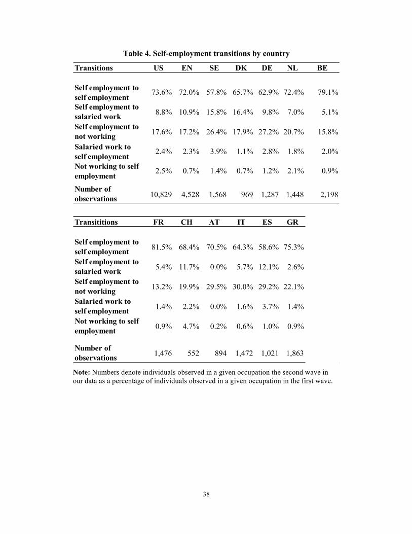
Tables 3 and 4 show transitions in occupational status that are observed in our data.
When we compute transition probabilities from period 𝑡 to period 𝑡 + 1 for different
occupational choices (shown in Table 3), we find that conditional of being self-employed

7
in the first period, there is a 70.7% chance of remaining self-employed in the next period
while there is a 20.9% chance of leaving work altogether. Switching from salaried
employment in the first period to self-employment in the next period has a probability of
2.31%. Conditional on not working in the first period, there is only a 1.61% chance to
become self-employed in the next period. We find that conditional of being self-
employed in the first period, the chance of remaining self-employed in the next period is
about 74.6% for men and about 63.9% for women. Except for the probability of staying
self-employed from one period to the next, the rest of transitions in and out of
occupations are similar between men and women.
Table 4 shows occupational transitions by country. The countries with higher
transitions from self-employment in period 𝑡 to also self-employment in period 𝑡 + 1 are
France (81.5%), Belgium (79.1%), Greece (75.3%) and the US (73.6%). The countries
with the lowest such transitions are Sweden and Spain. However, the countries where the
switching from salaried employment period 𝑡 to self-employment in period 𝑡 + 1 are
more likely are Sweden (3.9%) and Spain (3.7%). Transitioning from self-employment
into not working is high in Austria, Italy and Spain. We find that countries where
becoming a salaried worker in period 𝑡 + 1 conditional on being a self-employed worker
in period 𝑡 is more likely are Sweden and Denmark, while the lower rates of such
transitions are observed in Greece (2.6%) and Belgium (5.1%).
Turning now to factors that can affect self-employment transitions, we first
examine factors that refer to labor market policies. These include employment protection
laws, spending on labor market incentives (for employment, unemployment benefits, and
early retirement), expressed as the share of GDP devoted to such expenditures in each

8
country. The relationship of these factors to self-employment rates (but not to transitions
into and out of self-employment) has been examined in a number of previous studies.6
The objective of this study is to see whether they can also shed light into the transition
from salaried work to self-employment as well as to the transition from self-employment
to retirement.
We use information on the aforementioned variables that is provided by the OECD
at the country level (e.g. incentives on early retirement, again expressed as a share of
GDP), except for a variable that denotes the prevalence of the rule of law that is taken
from the World Bank database. Existing literature suggests that the rule of law affects
various parts of the economy as well as entrepreneurship in particular (see Djankov, La
Porta, Lopez-De-Silanes, Shleifer, 2002 and Aides et al., 2009).
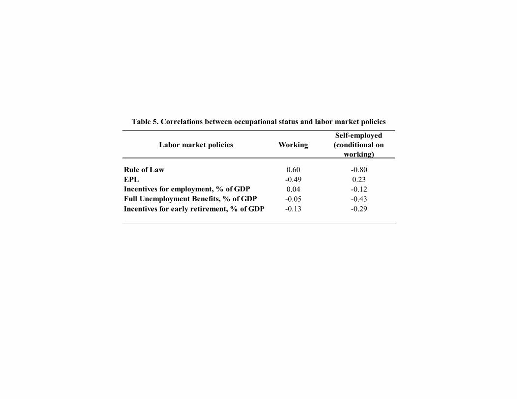
Table 4 displays the correlations between working and self-employment with the
five institutional variables used on our empirical specifications. There is a positive
correlation between the rule of law and working in any capacity and a strong negative
correlation with self-employment conditional on working. The same pattern is found with
incentives for employment. Stronger employment protection laws (EPL) have a negative
correlation with working but a positive one with self-employment. Higher unemployment
benefits are slightly negatively correlated with working in any capacity and also
negatively correlated with self-employment, and a similar pattern exists with respect to
incentives for early retirement.
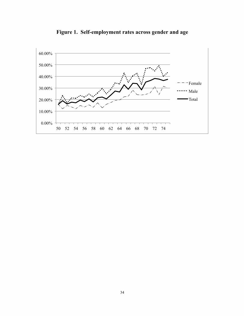
Self-employment is also correlated with a number of demographic characteristics.
As can be seen in Figure 1, and as already mentioned, the share of the self-employed
6 See e.g. Torrini, 2005; Parker and Robson, 2004; OECD, 2000). In particular, employment protection laws seem weakly correlated with self-employment rates (see Torrini, 2005; Robson, 2003). See also Carrasco (1999), and Carrasco and Ejrnæs (2003) for the case of unemployment benefits.

9
among those working rises with age. Several studies have already discussed this
empirical pattern (e.g. Blanchflower, 2000, Hochguertel, 2005), and different
explanations for it have been proposed. For example, one reason why self-employment
becomes more common with age could be the fact that it has features that are valuable to
older workers and that are not found in traditional salaried jobs, e.g. flexibility in working
hours.
The effect of health in employment can be very important given that older
individuals experience significant changes in their health, and given that self-employment
is particularly sensitive to health status (see Bound et al., 1999; Zissimopoulos and
Karoly, 2007; Parker and Rougier, 2007). We use the subjective self-reported health
status as an indicator of the health status of our sample respondents. Self-rated health was
measured by asking respondents to rate their health on a five-point scale: excellent, very
good, good, fair, poor. We define a binary variable denoting bad health, which takes the
value of one if the self-rated health is fair or poor, and zero otherwise.
We also check the effect of cognition on self-employment by using the score on
an immediate recall test7. Given that there is empirical evidence that points to the
importance of mental health in labor market transitions (Thomas et al., 2005, and Repetti
et al., 1985, for women), we include an indicator for whether the person is feeling
depressed. Finally, we also include in our empirical specifications variables denoting
being in couple, the number of children and grandchildren and education. We break
education into three levels, namely less than high-school, completed high-school and at
least some post-secondary education.
7 Interviewees are read ten words and are then asked to repeat them. The score in the test equal to the number of words correctly recalled.

10
3. Empirical Methodology8
3.1. Methodologies applied to estimate transition probabilities in discrete choice
models
There are several approaches that have been used in the literature to estimate
occupational transition probabilities. One approach is to start with a sample of working
individuals, and then define a binary variable that takes the value one if self-employed
and zero otherwise. This approach is problematic, however, as it starts with a potentially
very selected sample, i.e. those who work; the problem of selectivity would be
particularly severe when examining older individuals, as those who work in older age are
likely to be quite different from those who do not.
An alternative approach would be to use the whole sample (i.e., the self-employed,
the dependent workers and the retired) in a panel setting. Then for each employment
status there would be several transitions out of and into it, and the estimation could in
principle be done with a multinomial logit using each transition type as a different
outcome. However, some of the transitions would be irrelevant for some categories of
employment. For example, a transition from wage labor at time 𝑡 to self-employment at
𝑡 + 1 would be irrelevant for those who are self-employed at period 𝑡. This irrelevance
implies that there is no possibility to choose some of the outcomes in each period, which
would be a violation of the assumptions of the multinomial logit.
8 This section is based on Christelis and Fonseca (2015).
11
One could also study self-employment transitions by using a lagged dependent
variable in simple probit/logit or multinomial logit models. This would require, however,
the availability of at least three longitudinal waves. Furthermore, a lagged dependent
variable does not always warrant inclusion in a panel specification, and can create
additional problems in estimation.
Finally, one could also use a nested logit, but one of the assumptions in such a
model would be that unobservables of choices in different nests are uncorrelated with
each other, which is a rather implausible assumption in our context.
In order to address the above issues, we use the empirical model in Christelis and
Fonseca (2015), which allows us to compute transitions as conditional probabilities
naturally arising from a discrete choice panel data model. Importantly, this model takes
into account selectivity in the sample of older workers, and uses the autocorrelation of all
time-varying unobservable factors to construct the transition probabilities. Given that this
model does not require the use of a lagged dependent variable, it can also be used if one
has only two panel waves available, as is the case with our study.
3.2. Empirical strategy
Our approach to the problem with estimating transitions starts from the
specification of the individual’s decision problem. We posit that the individual first
chooses whether to work or not, and then, conditional on working, chooses whether to be
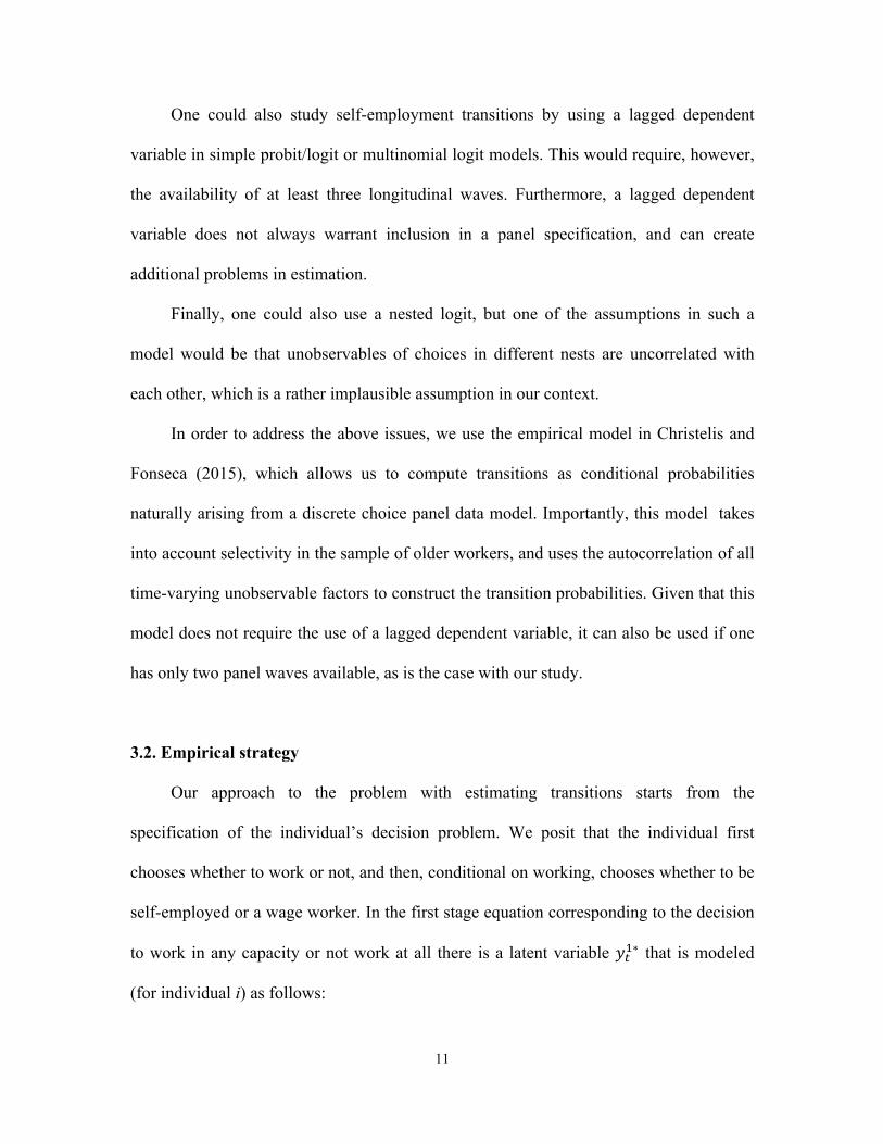
self-employed or a wage worker. In the first stage equation corresponding to the decision
to work in any capacity or not work at all there is a latent variable 𝑦!!∗ that is modeled
(for individual i) as follows:
12
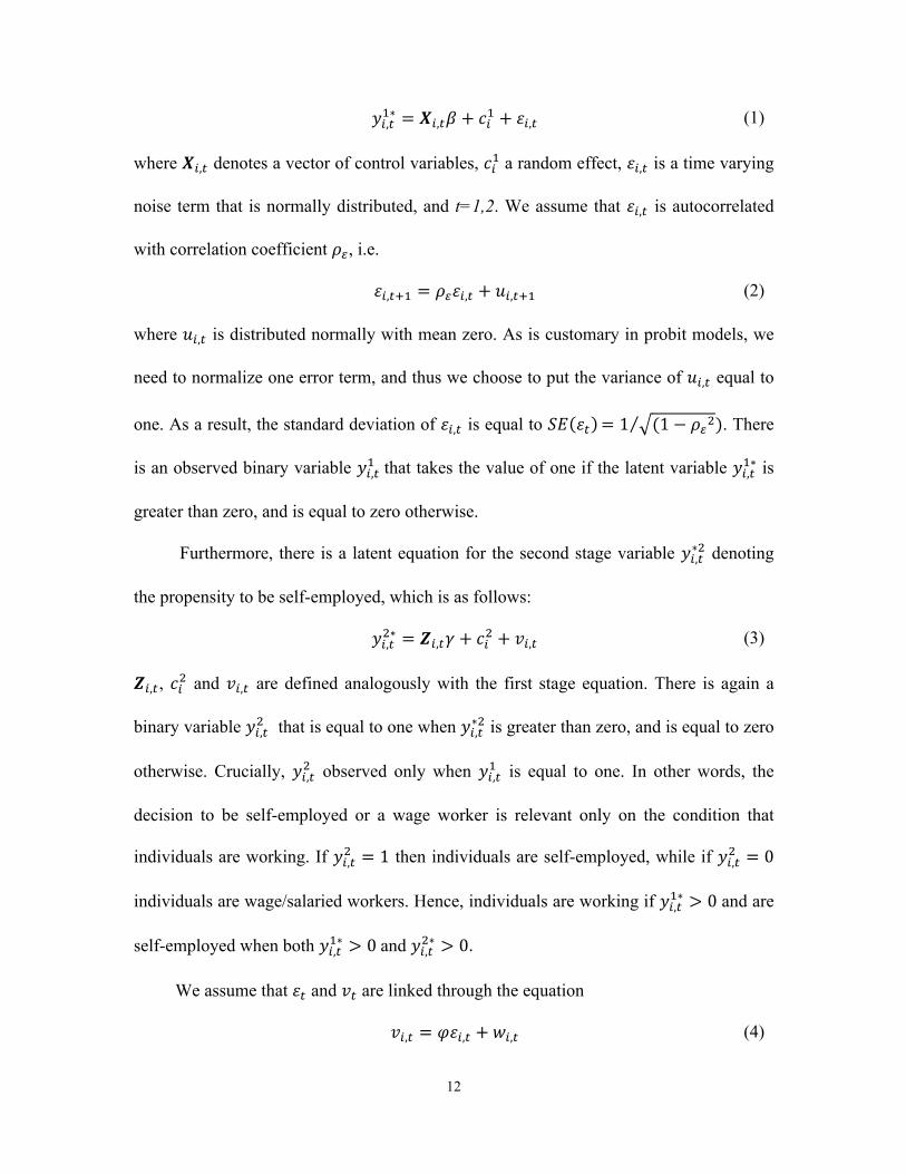
𝑦!,!!∗ = 𝑿!,!𝛽 + 𝑐!! + 𝜀!,! (1)
where 𝑿!,! denotes a vector of control variables, 𝑐!! a random effect, 𝜀!,! is a time varying
noise term that is normally distributed, and t=1,2. We assume that 𝜀!,! is autocorrelated
with correlation coefficient 𝜌!, i.e.
𝜀!,!!! = 𝜌!𝜀!,! + 𝑢!,!!! (2)
where 𝑢!,! is distributed normally with mean zero. As is customary in probit models, we
need to normalize one error term, and thus we choose to put the variance of 𝑢!,! equal to
one. As a result, the standard deviation of 𝜀!,! is equal to 𝑆𝐸 𝜀! = 1 (1− 𝜌!!). There
is an observed binary variable 𝑦!,!! that takes the value of one if the latent variable 𝑦!,!!∗ is
greater than zero, and is equal to zero otherwise.
Furthermore, there is a latent equation for the second stage variable 𝑦!,!∗! denoting
the propensity to be self-employed, which is as follows:
𝑦!,!!∗ = 𝒁!,!𝛾 + 𝑐!! + 𝑣!,! (3)
𝒁!,!, 𝑐!! and 𝑣!,! are defined analogously with the first stage equation. There is again a
binary variable 𝑦!,!! that is equal to one when 𝑦!,!∗! is greater than zero, and is equal to zero
otherwise. Crucially, 𝑦!,!! observed only when 𝑦!,!! is equal to one. In other words, the
decision to be self-employed or a wage worker is relevant only on the condition that
individuals are working. If 𝑦!,!! = 1 then individuals are self-employed, while if 𝑦!,!! = 0
individuals are wage/salaried workers. Hence, individuals are working if 𝑦!,!!∗ > 0 and are
self-employed when both 𝑦!,!!∗ > 0 and 𝑦!,!!∗ > 0.
We assume that 𝜀! and 𝑣! are linked through the equation
𝑣!,! = 𝜑𝜀!,! + 𝑤!,! (4)
13
where 𝑤!,! is distributed normally with mean zero. As was the case with the first stage
equation, we normalize the variance of 𝑤!,! to one.
Christelis and Fonseca (2015) show how to calculate the likelihood function that
incorporates the autocorrelation in (2) and the selectivity in (4). In turn, the formulation
of this likelihood function also allows the computation of transition probabilities of any
choice of interest. Additional details about the construction of this likelihood function are
given in Appendix A.1.
3.2. Self-employment Transitions
For our purposes, what is crucial is that the model generated by (1)-(4) allows the
calculation of transition probabilities for the choices of interest. The study of transitions
comes naturally out of this setup if one considers that a transition probability is just a
conditional probability of an outcome at 𝑡 + 1 conditional on an outcome at 𝑡, and this is
equal to the joint probability of the two outcomes divided by the marginal probability of
the conditioning outcome at time 𝑡. The existence of 𝜌! implies that the joint probability
is not equal to the product of the marginal probabilities of the two outcomes, and thus the
conditional probability does not collapse to the marginal probability of the outcome at
𝑡 + 1.
3.3. Marginal effects
Our model is rich enough to allow us to calculate the marginal effects of our
variables of interest on the probabilities of: i) working (unconditional); ii) being self-
employed (unconditional); iii) being self-employed conditional on working; iv) being a
14
dependent worker (unconditional); v) being a dependent worker conditional on working;
vi) transitioning from not working to working; vii) transitioning from working to not
working; viii) transitioning from dependent work to self-employment; ix) transitioning
from not working to self-employment; x) transitioning from self-employment to not
working; xi) transitioning from self-employment to dependent work.
When calculating the marginal effects on transition probabilities, one can use a
couple of formulations of the marginal effect. First, one can calculate the conditional
probability for a given value of the forcing variable in both periods, then calculate the
same probability for a second value of the forcing variable (again constant across time)
and then take the difference of the two conditional probabilities. This calculation is
especially useful when one wants to compare indicators of labor market policies that take
different values across countries but do not change over time. It is also useful in the case
of variables that change very little or not at all over time in our sample of older
individuals (e.g. gender, education, number of children). We will call the marginal effect
resulting from this calculation a Type I marginal effect.
The second possibility is to calculate the conditional probability using a given value
of the forcing variable at 𝑡, and another value at 𝑡 + 1,9 and then compare the conditional
probability so calculated to a conditional probability where the forcing variable takes the
same value in both periods. For example, if one were interested in the effect of health
deterioration on the transition from self-employment to not working, one could evaluate
the conditional probability of this transition by putting the dummy for bad health equal to
zero at 𝑡 and equal to one at 𝑡 + 1, and then compare it with a conditional probability
9 When calculating the marginal effects of continuous variables, we change their levels by one standard deviation.
15
where the bad health dummy is equal to zero in both periods. This type of marginal effect
(which we call a Type II marginal effect) is especially useful for studying the effects of
common changes across countries in labor market policies and institutional factors from
one period to the next. These changes could be thought as policy experiments across
time. Type II marginal effects are also useful for studying the effects of changes in
variables that are likely to change from period to period in our sample, such as being in a
couple, bad health, being depressed, the number of grandchildren, cognition One should
also note that by calculating the Type II marginal effect we can avoid using in our
specification forcing variables defined as changes over time; rather we can work with
forcing variables in levels, and just change their values from one period to the other.
We estimate our marginal effects and their standard errors by simulation; the
procedure we follow is described in detail in Appendix A.2.
4. Empirical Results
As already mentioned, our model allows us to compute a large number of
probabilities of occupational transitions. Due to space limitations, we will focus our
attention on the probabilities of: i) working (unconditional); ii) being self-employed
(conditional on working); iii) transitioning from working in any capacity to not working
at all; iv) transitioning from wage/salaried work to self-employment; v) transitioning
from not working to self-employment; vi) remaining self-employed from one period to
the next; vii) transitioning from self-employment to not working. For the transition
probabilities iii)-vii) we will compute both Type I and Type II marginal effects (already
discussed in Section 4). Our aim is to document the associations of labor market policies,
16
institutions and other determinants with self-employment transitions in older age.
We will discuss marginal effects, as coefficient estimates in discrete choice models
are very hard to interpret economically, and are in any case identified only up to scale.
Before discussing the marginal effects, however, we note that there are two other crucial
parameters that are estimated in our model: a) the autocorrelation coefficient 𝜌! of the
first stage noise term; b) the correlation between the first and second stage noise terms
𝜌!" that denotes selectivity. We find that 𝜌! is equal to 0.84 and very strongly significant
(p-value = 0.00). This means that there is very strong temporal dependence affecting the
noise terms in both equations, and consequently (as discussed in Section 3 and Appendix
A.1) conditional probabilities that denote transitions can be quite different from the
marginal probabilities of the choice in 𝑡 + 1. Furthermore, 𝜌!" is estimated to be equal to
-0.538 with a p-value of 0.001, which points to the fact that workers are a selected
sample; therefore empirical analyses that truncate the sample based on employment
choices may produce inconsistent estimates.
4.1. Static probabilities of working and of being self-employed conditional on
working
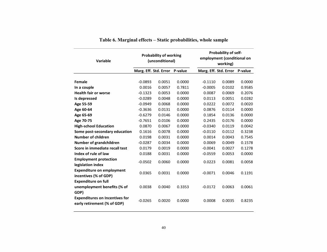
When we turn to the marginal effects on the unconditional probability of working,
(shown in Table 6), it is clear that the variables denoting labor market policies have
strong effects in the expected direction: a stronger rule of law and a larger spending for
incentives for employment increase the probability of working while stronger
employment protection and more generous incentives for early retirement reduce it.
Table 6 also shows the marginal effects on the probability of being self-employed
17
conditional on working, i.e. the probability that, once we know that a person is working,
she will be self-employed. These marginal effects show the influence of the variables of
interest on self-employment over and above the influence they have on the decision to
work or not. We find that three institutional variables matter for this conditional
probability of self-employment: large unemployment benefits and a stronger rule of law
make self-employment less likely, while the opposite is true for employment protection
legislation. Hence, it seems that stronger employment protection legislation hinders
salaried employment and thus turns those who want to work to become self-employed.
As for the rule of law, it appears that weaker law enforcement is an incentive for
becoming self-employed, probably because the self-employed can benefit from such
weaknesses more than salaried workers.
Table 6 shows very strong and significant negative effects on working of being a
female, in bad health and depressed, and of having more grandchildren. Furthermore,
there is a strong negative age gradient as expected. On the other hand, a higher education
and higher cognition affect employment positively. As for the probability of being self-
employed conditional on working, the age gradient is now positive, which means that
once a person is working at this age range, being older increases the chances of being
self-employed. This finding is consistent with a pattern of individuals turning to self-
employment before they retire completely. Furthermore, being a female lowers the
probability of being self-employed, while bad health does not affect it.
4.2. Transitions into and out of self-employment when covariates are considered
time invariant
18
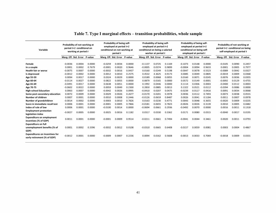
Most of the added value of our econometric model, however, lies in the
computation of transition probabilities, as discussed in Section 3. We begin with the Type
I marginal effects on the probability of transitioning from (i) working to not working; (ii)
not working to self-employment, (iii) from salaried work to self-employment, (iv) from
self-employment to self-employment and iv) from self-employment to not working.
Given that Type I marginal effects refer to situations in which covariates do not change
between periods, the effects of labor market policies in this case should be interpreted as
differences among countries exhibiting higher and lower values of the associated
variables.
Results in Table 7 suggest that countries with a stronger rule of law exhibit a higher
probability of transitioning from any type of work to no work, a lower probability of
switching from salaried work to self-employment, and of staying in self-employment.
These patterns could be due to the fact that self-employment is much more prevalent in
southern European countries where the rule of law is weaker.
In countries where employment protection legislation is stronger, the transition out
of work is less likely, which is probably one of the goals of such legislation. On the other
hand, employment protection is not in general associated with self-employment, although
it increases slightly the probability of transitioning out of it into not working at all.
Similarly, countries with differences in spending on employment incentives do not seem
to differ with respect to self-employment transition probabilities.
On the other hand, more generous unemployment benefits are negatively associated
with self-employment, as countries that spend more on them exhibit lower probabilities
of becoming self-employed when not working and of staying self-employed from one

19
period to the next. Finally, incentives for early retirement are associated with a slightly
higher probability of transitioning from self-employment to not working.
When examining the associations of demographic characteristics with self-
employment, we again examine situations in which the values of these characteristics do
not change over time. Hence the interpretation of the marginal effects in this case is the
difference in the probabilities of the outcomes among individuals exhibiting different
values of these variables.
As expected, age has a strong negative association with being employed, but a very
strong positive one with self-employment, conditional on working. In addition, we find
that being a female, and in bad health make transitions out of work more likely,
transitions into self-employment less likely, and transitions out of it more likely. On the
other hand we find no economically significant associations of self-employment with
depression, having children and grandchildren, or having a better memory.
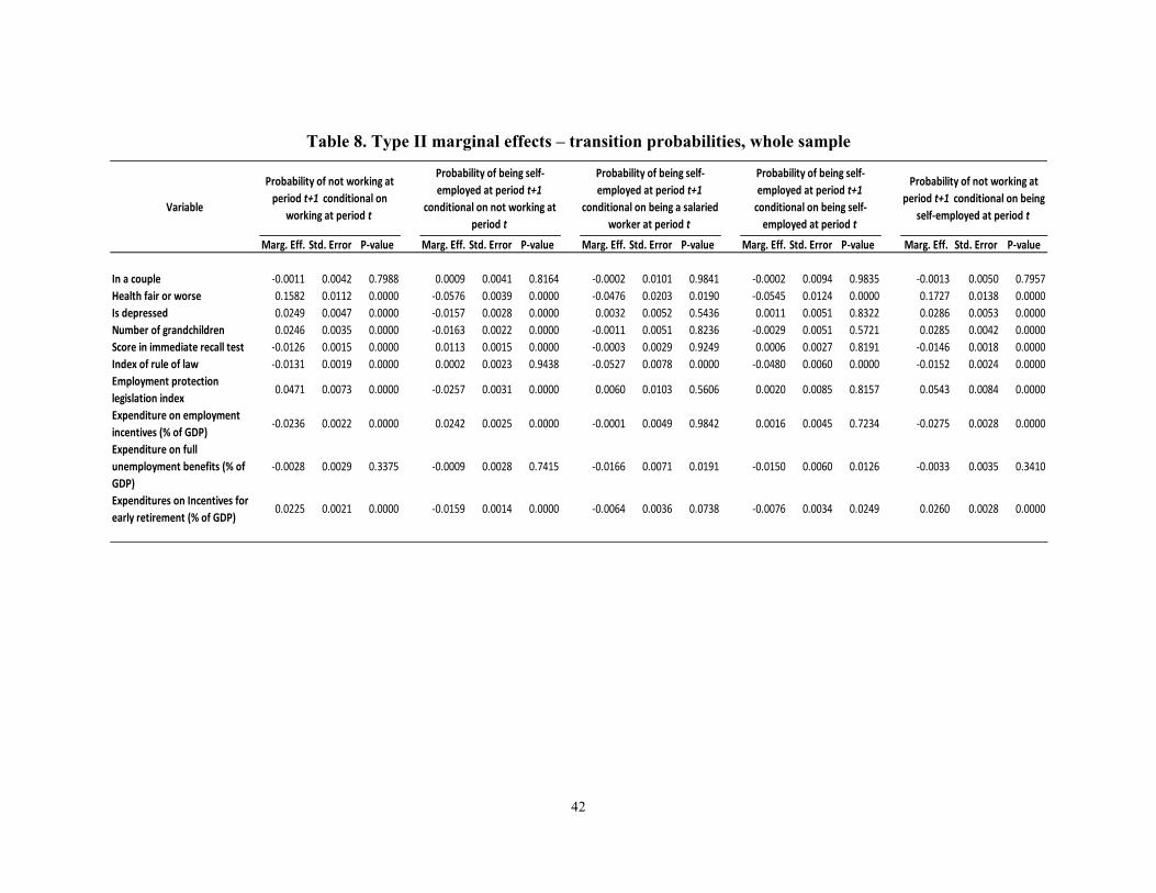
4.3. Transitions into and out of self-employment when covariates change over time
We turn now to Type II marginal effects, i.e. marginal effects that are due to a
change in the variables of interest from 𝑡 to 𝑡 + 1. Hence, the marginal effects of the
country-level labor market policy variables should be now interpreted as indicating what
happens on average if those variables change from one period to the next by the same
amount in all countries. We show these marginal effects in Table 8.
An increased strength in the rule of law is associated with a higher probability of
transitioning from any type of work to no work, lower probabilities of switching into self-
employment, and of staying in self-employment. Hence, the negative association of the

20
rule of law with self-employment is present also across time, and not only across
countries.
Incentives on employment seem to be particularly effective, as an increase in the
share of GDP devoted to these expenditures is associated with lower probabilities of
transitioning out of work, higher probabilities of transitioning into self-employment, and
lower probabilities of transitioning out of it. On the other hand, and as expected, an
increase in the strength of employment protection legislation has exactly the opposite
effects.
An increase in the share of GDP devoted to unemployment benefits is negatively
associated with self-employment, as it is has a negative effect on the probabilities of
becoming self-employed when not working and of staying self-employed from one
period to the next.
Incentives for early retirement have strong effects that go in the expected direction,
as an increase in the share of GDP devoted to them is associated with more likely
transitions out work, less likely transitions into self-employment, shorter spells of self-
employment, and higher probabilities of transitioning out of self-employment.
When examining the associations of demographic characteristics with self-
employment, we now examine (as opposed to what was done in Section 4.3) situations in
which the values of these characteristics change over time. Hence the interpretation of the
marginal effects in this case is the average change in the probability of the outcomes
when those variables change values by the same amount between periods for all
individuals in the sample.
We find that a deteriorating physical and mental health make transitions out of

21
work more likely, transitions into self-employment less likely and transitions out of it
more likely. We also find negative associations of having a grandchild with self-
employment. On the other hand, a higher cognition is associated with less likely
transitions out of work, more likely transitions into self-employment and less likely
transitions out of it.
All in all, the picture that emerges from both Type I and Type II marginal effects of
both labor market and demographic variables is that they generally go in the expected
direction and are economically relevant. Hence, our findings give no obvious indications
of severe misspecification problems in our empirical model.
6. Conclusions
In this paper we have studied transitions of older individuals in and out of self-
employment in thirteen OECD countries, focusing in particular on the effect of labor
market policies and institutional factors on these transitions. To that effect, we have
constructed an empirical model that separates the decision to work or not from the
decision to be self-employed, while taking into account both the intratemporal and,
crucially for the computation of transition probabilities, the intertemporal correlation of
the unobservables in both decisions. Furthermore, our model uses the whole sample and
the usual static outcomes as dependent variables, while also taking into account the panel
nature of our dataset.
Our results suggest that self-employment is strongly affected by government labor
market policies. Transitions into self-employment are positively associated with
expenditures on employment incentives, while they are negatively associated with the
strength of the rule of law and of employment protection legislation, and with

22
expenditure on early retirement incentives and on unemployment benefits.
In addition, our findings suggest that transitions in and out of self-employment are
affected by several demographic characteristics in more or less expected ways. For
example, good physical and mental health, higher cognition make it more likely that one
becomes and stays self-employed, while being a female, and having more grandchildren
have the opposite effect.
There is certainly scope for further research on both the empirical and on the
theoretical side about the precise ways with which labor market policies and retirement
reforms affect self-employment. In particular, models in which individuals’ objectives,
constraints, and influences by policy variables are explicitly modeled could be useful: for
example, for creating a number of counterfactual situations whose differing outcomes
could shed light on the effects of policy changes on self-employment. We leave this task
for future research.
23
References
Acemoglu, D., and S. Johnson (2005), “Unbundling Institutions.”, Journal of Political
Economy, 113: 949-995.
Ajayi-Obe, O. and S.C. Parker (2003), “The Changing Nature of Work among the Self-
Employed in the 1990s: Evidence from Britain”, Journal of Labor Research,
Transaction Publishers, vol. 26(3), pp. 501-517.
Blanchflower D. G. and A. Oswald (1998), "What makes an entrepreneur?", Journal of
Labor Economics, January, 16(1) pp. 26-60, 1998.
Blanchflower, D. (2000), “Self-employment in OECD countries.” Labour Economics 7:
471-505.
Been, J. and M. Knoef (2012), “Exit Routes to Retirement; the Role of Social Security
and Self-employment” mimeo.
Bound, J., Schoenbaum M., Stinebrickner T. R., and T. Waidmann (1999), “The
Dynamic Effects of Health on the Labor Force Transitions of Older Workers.”
Labour Economics, 6: 179–202.
Bruce, D., Holtz-Eakin D., and J. Quinn (2000). “Self-Employment and Labor Market
Transitions at Older Ages”. Boston College Center for Retirement Research Working
Paper No. 2000-13.
Carrasco, R. (1999). “Transitions to and from self-employment in Spain: an empirical
analysis”. Oxford Bulletin of Economic and Statistics, 61, pp. 315-41.
Carrasco, R. and M. Ejrnæs (2003) “Self-employment in Denmark and Spain: Institution,
Economic Conditions and Gender differences“ . mimeo.
24
Chamberlain, G. (1980), “Analysis of covariance with qualitative data.” Review of
Economic Studies 47, 225–238.
Chamberlain, G. (1984), “Panel Data.” In Handbook of Econometrics, Vol. 2, Z. Griliches
and M.D. Intriligator (eds). Elsevier Science.
Christelis, D. and Fonseca, R. (2015). “Transition probabilities in discrete choice panel
data models with autocorrelation and selectivity”. Mimeo.
Cowling, M. (2000). “Are entrepreneurs different across countries?” Applied Economics
Letters, 7:785–789.
Fonseca, R., P.C. Michaud and T. Sopraseuth (2007), “Entrepreneurship, wealth,
liquidity constraints and start-up costs”, Comparative Labor Law and Policy Journal,
2007, 28 (4), Summer issue.
Fuchs, V. (1982), “Self-employment and labor force participation of older males.”
Journal of Human Resources 17: 339-357.
Djankov, S., La Porta, R., Lopez-De-Silanes, F. & Shleifer A. (2002). “The Regulation of
Entry.”, The Quarterly Journal of Economics, MIT Press, vol. 117(1): 1-37.
Guiso, L., Sapienza, P. & Zingales, L. (2009). “Cultural Biases in Economic Exchange”,
Quarterly Journal of Economics 124(3), 1095-1131.
Geweke J. (1989). “Bayesian inference in econometric models using Monte Carlo
integration.” Econometrica, 57: 1317–1339.
Giandrea, M. D., Cahill, K.E., and J. F. Quinn (2008), “Self-Employment Transitions
among Older American Workers with Career Jobs.” Bureau of Labor Statistics
Working Paper 418.

25
Heckman, J., and Singer (1984). “A Method for Minimizing the Impact of Distributional
Assumptions in Econometric Models for Duration Data”, Econometrica, 52(2), 271-
320.
Henley, A. (2007). “Entrepreneurial aspiration and transition into self-employment:
evidence from British longitudinal data”, Entrepreneurship&Regional Development,
19(3), pp. 51-66.
Hochguertel, S. (2005), “Self-Employment around Retirement in Europe.” Economy,
112(2): 319-347.
Holtz-Eakin, D., D. Joulfaian, and H. S. Rosen (1994), “Entrepreneurial Decisions and
Liquidity Constraints”, The RAND Journal of Economics, 25, 334.347.
Hyytinen, A. and Rouvinen, P. (2008) “The labour consequences of self-employment
spells: European evidence.” Labour Economics, Elsevier, vol. 15(2), pages 246-271.
Jenkins, S.P., Capellari, L., Lynn, P., Jäckle, A., and E. Sala (2006). “Patterns of consent:
evidence from a general household survey.” Journal of the Royal Statistical Society
A, 169: 701-722.
Keane M. (1992). "A Note on Identification in the Multinomial Probit Model" Journal of
Business & Economic Statistics, 10(2), 193-200.
Keane M. (1994). “A computationally practical simulation estimator for panel data.”
Econometrica, 62: 95–116.
Michaud, P.C., and K. Tatsiramos (2008), “Fertility and Female Employment Dynamics
in Europe: The Effect of Using Alternative Econometric Modeling Assumptions”,
Journal of Applied Econometrics. John Wiley & Sons, Ltd., vol. 26(4), pages 641-
668, 06.

26
Mroz, T.A. (1999), “Discrete factor approximations in simultaneous equation models:
Estimating the impact of a dummy endogenous variable on a continuous outcome.”
Journal of Econometrics, 92: 233-274.
Mundlak, Y. (1978). “On the pooling of time series and cross sectional data.”
Econometrica 56, 69–86.
OECD (2000). The Employment Outlook. OECD, Paris.
Parker, S.C., and M.T. Robson (2004). Explaining international variations in self-
employment: evidence from a panel of OECD countries”, Southern Economic
Journal, 71, pp. 287-301.
Parker, S.C., and J. Rougier (2007), “The Retirement Behaviour of the Self-employed in
Britain”, Applied Economics, Taylor & Francis Journals, vol. 39(6), pages 697-713.
Quinn, J. (1980) “Labor force participation patterns of older self-employed workers.”
Social Security Bulletin, 43: 17-28.
Robson, M.T. (2003). “Does stricter employment protection legislation promote self-
employment?” Small Business Economics 21, 309 – 319
Repetti R. L., Matthews, K.A., and I. Waldron (1989) “Effects of Paid Employment on
Women's Mental and Physical Health.” American Psychologist 44(11): 1394-1401.
Rosti, L. and F. Chelli (2005), “Gender Discrimination, Entrepreneurial Talent and Self-
Employment”, J Small Business Economics, Vol. 24, n2, pp. 131-142
Thomas, C., Benzeval M., and S. A. Stansfeld (2005) “Employment transitions and
mental health: an analysis from the British household panel survey.” J Epidemiol
Community Health 2005; 59:243–249.
Torrini, R. (2005). “Cross-country differences in self-employment rates: the role of

27
institutions” Labour Economics, 12: 661 – 683
Train, K. (2003). Discrete Choice Methods with Simulation. Cambridge: Cambridge
University Press.
Wellington, A. (2006), “Self-employment: the new solution for balancing family and
career?”, Labour Economics, Vol. 13, Issue 3, June 2006, pp. 357-386.
Zissimopoulos, J., and Karoly, L. (2007) “Transitions to self-employment at older ages:
The role of wealth, health, health insurance and other factors.” Labour Economics,
14:269-95.
Zissimopoulos, J., Maestas, N., and Karoly, L. (2006) “The Effect of Retirement
Incentives on Retirement Behavior: Evidence from the Self-Employed in the United
States and England.” RAND Working Paper #WR-528, 2006.

28
Appendix
A.1 Likelihood function and transition probabilities
Clearly, the parameter φ in (4) is the source of the selectivity affecting the self-
employment/wage labor decision in the second stage equation (3). Proposition 1 (see
Christelis and Fonseca, 2015, for a proof,) establishes the correlations between the
unobservables in equations (1) and (3), as well as the variance of 𝑣!:
Proposition 1: The unobservables 𝜀! , 𝜀!!! , 𝜀! , 𝑣!!! have the following correlations:
a) 𝐶𝑜𝑟𝑟 𝜀! , 𝑣! = 𝜌!" = 𝜑/ 𝜑! + 1− 𝜌!!
b) 𝐶𝑜𝑟𝑟 𝑣!!!, 𝑣! = 𝜌! = 𝜑!𝜌!/ 𝜑! + 1− 𝜌!!
c) 𝐶𝑜𝑟𝑟 𝑣!!!, 𝜀! = 𝐶𝑜𝑟𝑟 𝜀!!!, 𝑣! = 𝜏!" = 𝜑𝜌!/ 𝜑! + 1− 𝜌!!
In addition, 𝑣! has a variance equal to 𝑉𝑎𝑟 𝑣! = (𝜑! + 1− 𝜌!!) (1− 𝜌!!)
Hence, the parameters φ and 𝜌! fully pin down all correlations between the time-
varying error terms, including the autocorrelation of the error term 𝑣 of the second stage
equation.
We also assume that 𝑐!! and 𝑐!! take values from two distributions with 𝐾 points
each (the first point is normalized to zero in both cases as in Michaud and Tatsiramos,
2008), and for each point (𝑘 = 1,… ,𝐾), there is an associated probability 𝑝! that is
common to both 𝑐!! and 𝑐!!. In other words, we estimate a non-parametric distribution for
the two-dimensional random effect, as in Heckman and Singer (1984). The use of a non-
parametric distribution for the random effects should increase the robustness of our

29
results (Mroz, 1999).10
It is quite important to model the random effects separately from the noise terms
for yet another reason: if one merged the random effects with the noise terms to produce
a composite time-varying term, this latter term would have a component with an
autocorrelation equal to one (i.e., the random effect), and this could in practice limit the
range of the autocorrelation coefficients of the noise terms. Therefore, modeling
separately the random effects and the noise terms makes our model more flexible.
All the above imply that the probability of observing any combination of the four
possible choices (two decisions in each of the two periods in our sample) can be
written11, for a given point 𝑘 of the two-dimensional distribution of the random effects, as
ℎ 𝒚! 𝑿! ,𝒁! , 𝒄! =
Φ!𝑙! 𝑿!,!𝜷+ 𝑐!! /𝑆𝐸 𝜀!,! ,𝑚! 𝒁!,!𝜸+ 𝒄!! /𝑆𝐸 𝑣!,! ,
𝑙!!! 𝑿!,!!!𝜷+ 𝑐!! /𝑆𝐸 𝜀!,!!! ,𝑚!!! 𝒁!,!!!𝜸+ 𝒄!! /𝑆𝐸 𝑣!,!!! ,𝜔
(A.1)
where 𝒚! = 𝑦!!, 𝐼 𝑦!!∗ 𝑦!!,𝑦!!!! , 𝐼 𝑦!!!!∗ 𝑦!!!! , 𝑿! = 𝑿!,! ,𝑿!,!!! , 𝒁! = 𝒁!,! ,𝒁!,!!! ,
𝑙! = ±1, 𝑙!!! = ±1, 𝑚! = ±1 if 𝑙! = 1 and 𝑚! = 0 otherwise, 𝑚!!! = ±1 if 𝑙!!! = 1
and 𝑚!!! = 0 otherwise, 𝒄! = 𝑐!!, 𝑐!! ,
𝜔 = 𝑙!𝑚!𝜌!" , 𝑙!𝑙!!!𝜌! , 𝑙!𝑚!!!𝜏!" , 𝑙!!!𝑚!𝜏!" ,𝑚!𝑚!!!𝜌! , 𝑙!!!𝑚!!!𝜌!" , Φ! denotes the
𝑝-dimensional normal cumulative distribution, with 𝑝 = 𝑙! + 𝑚! + 𝑙!!! + 𝑚!!! .
The 𝑝-dimensional normal integral in (6) is estimated by simulated maximum
likelihood, using the Geweke-Hadjivassiliou-Keane simulator (Geweke, 1989; Keane,
1994). The dimension of the integral varies according to the choices observed in the first
stage decisions at 𝑡 and 𝑡 + 1. It is equal to two when the person does not work in either
10 We currently use two distribution points for each of the two random effects. 11 We use the formulation by Jenkins et al. (2009).

30
period, equal to three if she works in one of the two periods, and equal to four when she
works in both periods. As a result, the likelihood term for each individual is that of a
multivariate probit with the number of equations ranging from two to four.
All the above imply that the log likelihood of our sample can be written as
𝑙𝑛𝐿 = 𝑙𝑜𝑔 𝑝! ℎ(𝒚!|𝑿! ,𝒁! , 𝒄!
!
!!!
!
!!!
(A.2)
Equation (A.1) in turn implies that one can calculate transition probabilities of any
combination of choices. As an example, the probability of transitioning from self-
employment at time 𝑡 to not working at time 𝑡 + 1 is given by
𝑃𝑟𝑜𝑏 𝑦!!!! = 0|𝑦!! = 0,𝑦!! = 0 =
𝑝!Φ!
𝑿!,!𝜷+ 𝑐!!
𝑆𝐸 𝜀!,!,𝒁!,!𝜸+ 𝒄!!
𝑆𝐸 𝑣!,!,− 𝑿!,!!!𝜷+ 𝑐!!
𝑆𝐸 𝜀!,!!!,𝜌!" ,−𝜌!, − 𝜏!"
Φ!𝑿!,!𝜷+ 𝑐!!
𝑆𝐸 𝜀!,!,𝒁!,!𝜸+ 𝒄!!
𝑆𝐸 𝑣!,!,𝜌!"
!
!!!
(A.3)
i.e., by integrating over the distribution of the random effects the joint probability of
working at 𝑡, being self-employed at 𝑡, and not working at 𝑡 + 1, divided by the joint
probability of working and being self-employed at 𝑡.
It is worth noting that the term multiplied by 𝑝! in (5) is defined for any given
values of the two random effects 𝑐!and 𝑐!, i.e., the fact that we can use joint probabilities
to calculate transition probabilities is due solely to the existence of 𝜌!. If 𝜌! were equal to
zero, the conditional probability in (A.3) would collapse to the marginal probability of
the outcome at 𝑡 + 1 for all values of the random effects. This would be so because in the
case of 𝜌! equal to zero the numerator would be equal to the probability of not working at
𝑡+1 multiplied by the probability of being self-employed at 𝑡. On the other hand, if φ
31
were equal to zero but 𝜌! different from zero, the conditional probability in (8) would still
be different from the marginal probability of the outcome at 𝑡 + 1. In other words,
selectivity is not necessary for the existence of non-trivial transition probabilities,
although its presence obviously affects their value.
Let us also emphasize that conditional probabilities like the one shown in (A.3) do
not require an outcome defined as a transition but are derived naturally from the
combinations of the static outcomes while taking into account all possible sources of
correlation in the noise terms.
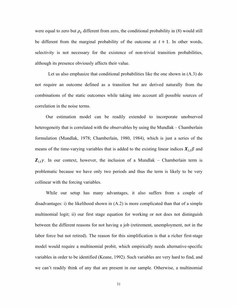
Our estimation model can be readily extended to incorporate unobserved
heterogeneity that is correlated with the observables by using the Mundlak – Chamberlain
formulation (Mundlak, 1978; Chamberlain, 1980, 1984), which is just a series of the
means of the time-varying variables that is added to the existing linear indices 𝑿!,!𝛽 and
𝒁!,!𝛾. In our context, however, the inclusion of a Mundlak – Chamberlain term is
problematic because we have only two periods and thus the term is likely to be very
collinear with the forcing variables.
While our setup has many advantages, it also suffers from a couple of
disadvantages: i) the likelihood shown in (A.2) is more complicated than that of a simple
multinomial logit; ii) our first stage equation for working or not does not distinguish
between the different reasons for not having a job (retirement, unemployment, not in the
labor force but not retired). The reason for this simplification is that a richer first-stage
model would require a multinomial probit, which empirically needs alternative-specific
variables in order to be identified (Keane, 1992). Such variables are very hard to find, and
we can’t readily think of any that are present in our sample. Otherwise, a multinomial
32
probit can in principle be incorporated in the multivariate normal framework shown in
(3), albeit at the cost of increasing the dimension of the integral compared to using a
simple probit to model the decision to work or not. This would make the convergence of
an already very complicated likelihood function even more difficult.
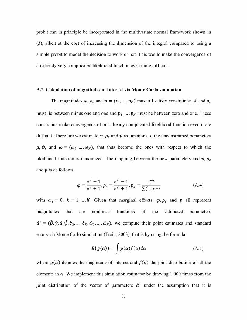
A.2 Calculation of magnitudes of Interest via Monte Carlo simulation
The magnitudes 𝜑, 𝜌! and 𝒑 = (𝑝!,… ,𝑝!) must all satisfy constraints: φ and 𝜌!
must lie between minus one and one and 𝑝!,… ,𝑝! must be between zero and one. These
constraints make convergence of our already complicated likelihood function even more
difficult. Therefore we estimate 𝜑, 𝜌! and 𝒑 as functions of the unconstrained parameters
𝜇, 𝜓, and 𝝎 = (𝜔!,… ,𝜔!), that thus become the ones with respect to which the
likelihood function is maximized. The mapping between the new parameters and 𝜑, 𝜌!
and 𝒑 is as follows:
𝜑 =
𝑒! − 1𝑒! + 1 ,𝜌! =
𝑒! − 1𝑒! + 1
,𝑝! =𝑒!!
𝑒!!!!!!
(A.4)
with 𝜔! = 0, 𝑘 = 1,… ,𝐾. Given that marginal effects, 𝜑, 𝜌! and 𝒑 all represent
magnitudes that are nonlinear functions of the estimated parameters
𝛼∗ = (𝜷,𝜸, 𝜇,𝜓, 𝒄!,… , 𝒄! ,𝜔!,… ,𝜔!), we compute their point estimates and standard
errors via Monte Carlo simulation (Train, 2003), that is by using the formula
𝐸 𝑔 𝛼 = 𝑔 𝛼 𝑓 𝛼 𝑑𝛼 (A.5)
where 𝑔 𝛼 denotes the magnitude of interest and 𝑓 𝑎 the joint distribution of all the
elements in 𝛼. We implement this simulation estimator by drawing 1,000 times from the
joint distribution of the vector of parameters 𝛼∗ under the assumption that it is
33
asymptotically normal with mean and variance-covariance matrix equal to the maximum
likelihood estimates. For a given parameter draw j we generate the magnitude of interest
𝑔 𝛼∗! . For marginal effects in particular, we first calculate the partial effect
corresponding to each individual in our sample and then calculate the marginal effect
𝑔 𝛼∗! as the weighted average (using sample weights) of the effect across individuals.12
We then estimate 𝐸 𝑔 𝛼 and its standard error as the mean and standard deviation
respectively of the distribution of 𝑔 𝛼∗! over all parameter draws.
12 We do not evaluate marginal effects at sample means since this practice can lead to severely misleading results (see Train, 2003, pp. 33-34).
34
Figure 1. Self-employment rates across gender and age
0.00%
10.00%
20.00%
30.00%
40.00%
50.00%
60.00%
50 52 54 56 58 60 62 64 66 68 70 72 74
Female
Male
Total

35
Table 1. Descriptive statistics Variable Statistic
Is working for pay 45%Self-employed (conditional on working) 22%Age 62.3
50-54 17%55-59 25%60-64 20%65-69 18%70-75 15%
Female 53%Is in a couple 72%No of children 2.56No of grandchildren 3.31Less than high school 30%High School Education 33%Post-secondary education 36%Self-reported health fair or worse 28%Is Depressed 26%Immediate recall score 5.43
No of observations 67,108

36
Table 2. Occupational status by country and by gender
Country
Total Male Female Total Male FemaleUSA 54.04% 60.55% 48.30% 21.50% 26.34% 16.16%Sweden 55.63% 58.20% 53.00% 13.57% 19.04% 7.39%Denmark 51.64% 57.65% 45.39% 10.80% 13.61% 7.08%Germany 36.13% 39.11% 33.33% 17.37% 18.48% 16.15%Netherlands 39.43% 46.99% 32.19% 14.89% 14.40% 15.59%Belgium 30.22% 36.53% 23.99% 19.79% 21.75% 16.84%France 36.56% 38.64% 34.72% 15.53% 18.03% 13.06%Switzerland 59.06% 68.21% 50.25% 26.66% 31.25% 20.66%Austria 27.91% 35.07% 21.21% 17.22% 16.52% 18.31%Italy 25.21% 36.06% 15.72% 36.29% 45.20% 18.42%Spain 31.04% 40.11% 23.11% 28.03% 28.81% 26.86%Greece 31.74% 45.59% 19.31% 44.23% 49.11% 33.89%England 36.66% 42.55% 31.27% 18.00% 22.58% 12.31%
Working Self-employed (conditional on working)

37
Table 3. Self-employment transitions by gender, all countries
Transitions All Female Male
Self employment to self employment
70.68% 63.87% 74.57%
Self employment to salaried work
8.42% 8.71% 8.25%
Salaried work to self employment
2.31% 2.14% 2.48%
Not working to self employment
1.61% 1.49% 1.78%
Number of observations
30,105 16,930 13,175
Note: Numbers denote individuals observed in a given occupation the second wave in our data as a percentage of individuals observed in a given occupation in the first wave.
38
Table 4. Self-employment transitions by country
Transitions US EN SE DK DE NL BE
Self employment to self employment
73.6% 72.0% 57.8% 65.7% 62.9% 72.4% 79.1%
Self employment to salaried work 8.8% 10.9% 15.8% 16.4% 9.8% 7.0% 5.1%
Self employment to not working 17.6% 17.2% 26.4% 17.9% 27.2% 20.7% 15.8%
Salaried work to self employment
2.4% 2.3% 3.9% 1.1% 2.8% 1.8% 2.0%
Not working to self employment
2.5% 0.7% 1.4% 0.7% 1.2% 2.1% 0.9%
Number of observations 10,829 4,528 1,568 969 1,287 1,448 2,198
Transititions FR CH AT IT ES GR
Self employment to self employment 81.5% 68.4% 70.5% 64.3% 58.6% 75.3%
Self employment to salaried work 5.4% 11.7% 0.0% 5.7% 12.1% 2.6%
Self employment to not working 13.2% 19.9% 29.5% 30.0% 29.2% 22.1%
Salaried work to self employment 1.4% 2.2% 0.0% 1.6% 3.7% 1.4%
Not working to self employment 0.9% 4.7% 0.2% 0.6% 1.0% 0.9%
Number of observations 1,476 552 894 1,472 1,021 1,863
Note: Numbers denote individuals observed in a given occupation the second wave in our data as a percentage of individuals observed in a given occupation in the first wave.
39
Table 5. Correlations between occupational status and labor market policies
Labor market policies WorkingSelf-employed (conditional on
working)
Rule of Law 0.60 -0.80EPL -0.49 0.23Incentives for employment, % of GDP 0.04 -0.12Full Unemployment Benefits, % of GDP -0.05 -0.43Incentives for early retirement, % of GDP -0.13 -0.29
40
Table 6. Marginal effects – Static probabilities, whole sample
Marg. Eff. Std. Error P-‐value Marg. Eff. Std. Error P-‐value
Female -‐0.0893 0.0051 0.0000 -‐0.1110 0.0089 0.0000In a couple 0.0016 0.0057 0.7811 -‐0.0005 0.0102 0.9585Health fair or worse -‐0.1323 0.0053 0.0000 0.0087 0.0069 0.2076Is depressed -‐0.0289 0.0048 0.0000 0.0113 0.0051 0.0282Age 55-‐59 -‐0.0949 0.0068 0.0000 0.0222 0.0072 0.0020Age 60-‐64 -‐0.3636 0.0131 0.0000 0.0876 0.0114 0.0000Age 65-‐69 -‐0.6279 0.0146 0.0000 0.1854 0.0136 0.0000Age 70-‐75 -‐0.7651 0.0106 0.0000 0.2435 0.0176 0.0000High-‐school Education 0.0870 0.0067 0.0000 -‐0.0340 0.0119 0.0042Some post-‐secondary education 0.1616 0.0078 0.0000 -‐0.0110 0.0112 0.3238Number of children 0.0198 0.0031 0.0000 0.0014 0.0043 0.7545Number of grandchildren -‐0.0287 0.0034 0.0000 0.0069 0.0049 0.1578Score in immediate recall test 0.0179 0.0019 0.0000 -‐0.0041 0.0027 0.1278Index of rule of law 0.0188 0.0031 0.0000 -‐0.0559 0.0053 0.0000Employment protection legislation index
-‐0.0502 0.0060 0.0000 0.0223 0.0081 0.0058
Expenditure on employment incentives (% of GDP)
0.0365 0.0031 0.0000 -‐0.0071 0.0046 0.1191
Expenditure on full unemployment benefits (% of GDP)
0.0038 0.0040 0.3353 -‐0.0172 0.0063 0.0061
Expenditures on Incentives for early retirement (% of GDP)
-‐0.0265 0.0020 0.0000 0.0008 0.0035 0.8235
Probability of working (unconditional)
Probability of self-‐employment (conditional on
working)Variable
41
Table 7. Type I marginal effects – transition probabilities, whole sample
Marg. Eff. Std. Error P-‐value Marg. Eff. Std. Error P-‐value Marg. Eff. Std. Error P-‐value Marg. Eff. Std. Error P-‐value Marg. Eff. Std. Error P-‐value
Female -‐0.0036 0.0004 0.0000 -‐0.0259 0.0034 0.0000 -‐0.1137 0.0725 0.1169 -‐0.1073 0.0148 0.0000 -‐0.0105 0.0090 0.2457In a couple 0.0001 0.0002 0.7679 -‐0.0001 0.0020 0.9646 -‐0.0005 0.0374 0.9899 -‐0.0004 0.0094 0.9633 0.0001 0.0005 0.7977Health fair or worse -‐0.0075 0.0007 0.0000 -‐0.0032 0.0016 0.0437 0.0160 0.0249 0.5198 -‐0.0047 0.0078 0.5523 -‐0.0089 0.0042 0.0327Is depressed -‐0.0012 0.0002 0.0000 0.0012 0.0010 0.2575 0.4532 4.3625 0.9173 0.0085 0.0049 0.0805 -‐0.0019 0.0009 0.0368Age 55-‐59 0.0094 0.0017 0.0000 0.0324 0.0029 0.0000 0.0189 0.0068 0.0055 0.0160 0.0071 0.0245 0.0076 0.0036 0.0355Age 60-‐64 -‐0.0114 0.0027 0.0000 0.0822 0.0055 0.0000 0.0879 0.0165 0.0000 0.0572 0.0149 0.0001 -‐0.0092 0.0129 0.4755Age 65-‐69 -‐0.0491 0.0017 0.0000 0.0638 0.0051 0.0000 0.1992 0.0446 0.0000 0.1114 0.0306 0.0003 -‐0.0400 0.0112 0.0003Age 70-‐75 -‐0.0602 0.0022 0.0000 0.0059 0.0049 0.2300 0.2850 0.0885 0.0013 0.1322 0.0521 0.0112 -‐0.0394 0.0086 0.0000High-‐school Education 0.0063 0.0007 0.0000 -‐0.0042 0.0026 0.0995 -‐0.0410 0.0207 0.0475 -‐0.0239 0.0117 0.0416 0.0091 0.0034 0.0068Some post-‐secondary education 0.0072 0.0009 0.0000 0.0029 0.0026 0.2677 -‐0.0170 0.0201 0.3978 0.0036 0.0112 0.7493 0.0073 0.0038 0.0555Number of children 0.0007 0.0001 0.0000 0.0010 0.0008 0.2446 -‐0.0126 0.0659 0.8487 0.0026 0.0041 0.5184 0.0011 0.0007 0.0978Number of grandchildren -‐0.0014 0.0002 0.0000 0.0003 0.0010 0.7826 0.0163 0.0230 0.4771 0.0043 0.0048 0.3655 -‐0.0020 0.0009 0.0235Score in immediate recall test 0.0006 0.0001 0.0000 -‐0.0001 0.0005 0.7866 -‐0.0181 0.0655 0.7823 -‐0.0026 0.0026 0.3139 0.0010 0.0005 0.0482Index of rule of law 0.0006 0.0001 0.0000 -‐0.0100 0.0014 0.0000 -‐0.0694 0.0661 0.2936 -‐0.0492 0.0070 0.0000 0.0016 0.0011 0.1318Employment protection legislation index
-‐0.0027 0.0005 0.0000 0.0025 0.0016 0.1182 0.0317 0.0330 0.3362 0.0171 0.0080 0.0315 -‐0.0040 0.0017 0.0195
Expenditure on employment incentives (% of GDP)
0.0011 0.0001 0.0000 -‐0.0001 0.0009 0.9514 -‐0.0211 0.0661 0.7494 -‐0.0041 0.0044 0.3461 0.0020 0.0011 0.0793
Expenditure on full unemployment benefits (% of GDP)
0.0001 0.0002 0.3396 -‐0.0032 0.0012 0.0108 -‐0.0310 0.0665 0.6408 -‐0.0157 0.0059 0.0081 0.0003 0.0004 0.4867
Expenditures on Incentives for early retirement (% of GDP)
-‐0.0012 0.0001 0.0000 -‐0.0009 0.0007 0.2236 0.0094 0.0162 0.5608 -‐0.0013 0.0033 0.7069 -‐0.0018 0.0009 0.0331
Probability of not working at period t+1 conditional on being
self-‐employed at period t
Probability of not working at period t+1 conditional on
working at period tVariable
Probability of being self-‐employed at period t+1
conditional on not working at period t
Probability of being self-‐employed at period t+1
conditional on being a salaried worker at period t
Probability of being self-‐employed at period t+1 conditional on being self-‐employed at period t
42
Table 8. Type II marginal effects – transition probabilities, whole sample
Marg. Eff. Std. Error P-‐value Marg. Eff. Std. Error P-‐value Marg. Eff. Std. Error P-‐value Marg. Eff. Std. Error P-‐value Marg. Eff. Std. Error P-‐value
In a couple -‐0.0011 0.0042 0.7988 0.0009 0.0041 0.8164 -‐0.0002 0.0101 0.9841 -‐0.0002 0.0094 0.9835 -‐0.0013 0.0050 0.7957Health fair or worse 0.1582 0.0112 0.0000 -‐0.0576 0.0039 0.0000 -‐0.0476 0.0203 0.0190 -‐0.0545 0.0124 0.0000 0.1727 0.0138 0.0000Is depressed 0.0249 0.0047 0.0000 -‐0.0157 0.0028 0.0000 0.0032 0.0052 0.5436 0.0011 0.0051 0.8322 0.0286 0.0053 0.0000Number of grandchildren 0.0246 0.0035 0.0000 -‐0.0163 0.0022 0.0000 -‐0.0011 0.0051 0.8236 -‐0.0029 0.0051 0.5721 0.0285 0.0042 0.0000Score in immediate recall test -‐0.0126 0.0015 0.0000 0.0113 0.0015 0.0000 -‐0.0003 0.0029 0.9249 0.0006 0.0027 0.8191 -‐0.0146 0.0018 0.0000Index of rule of law -‐0.0131 0.0019 0.0000 0.0002 0.0023 0.9438 -‐0.0527 0.0078 0.0000 -‐0.0480 0.0060 0.0000 -‐0.0152 0.0024 0.0000Employment protection legislation index
0.0471 0.0073 0.0000 -‐0.0257 0.0031 0.0000 0.0060 0.0103 0.5606 0.0020 0.0085 0.8157 0.0543 0.0084 0.0000
Expenditure on employment incentives (% of GDP)
-‐0.0236 0.0022 0.0000 0.0242 0.0025 0.0000 -‐0.0001 0.0049 0.9842 0.0016 0.0045 0.7234 -‐0.0275 0.0028 0.0000
Expenditure on full unemployment benefits (% of GDP)
-‐0.0028 0.0029 0.3375 -‐0.0009 0.0028 0.7415 -‐0.0166 0.0071 0.0191 -‐0.0150 0.0060 0.0126 -‐0.0033 0.0035 0.3410
Expenditures on Incentives for early retirement (% of GDP)
0.0225 0.0021 0.0000 -‐0.0159 0.0014 0.0000 -‐0.0064 0.0036 0.0738 -‐0.0076 0.0034 0.0249 0.0260 0.0028 0.0000
Probability of not working at period t+1 conditional on being
self-‐employed at period tVariable
Probability of not working at period t+1 conditional on
working at period t
Probability of being self-‐employed at period t+1
conditional on not working at period t
Probability of being self-‐employed at period t+1
conditional on being a salaried worker at period t
Probability of being self-‐employed at period t+1 conditional on being self-‐employed at period t


