
Linear algebra
& Numerical Analysis
Iterative methods
Marta Jarošová http://homel.vsb.cz/~dom033/

Outline
Direct and Iterative methods
Iterative process
Jacobi iterative method
Gauss-Seidel iterative method
Convergence theory

Iterative methods
Ax = b
Assumption: exist only one solution
Iterative solution procedure: generating sequence of
approximations {x(k)} of the solution
Example:
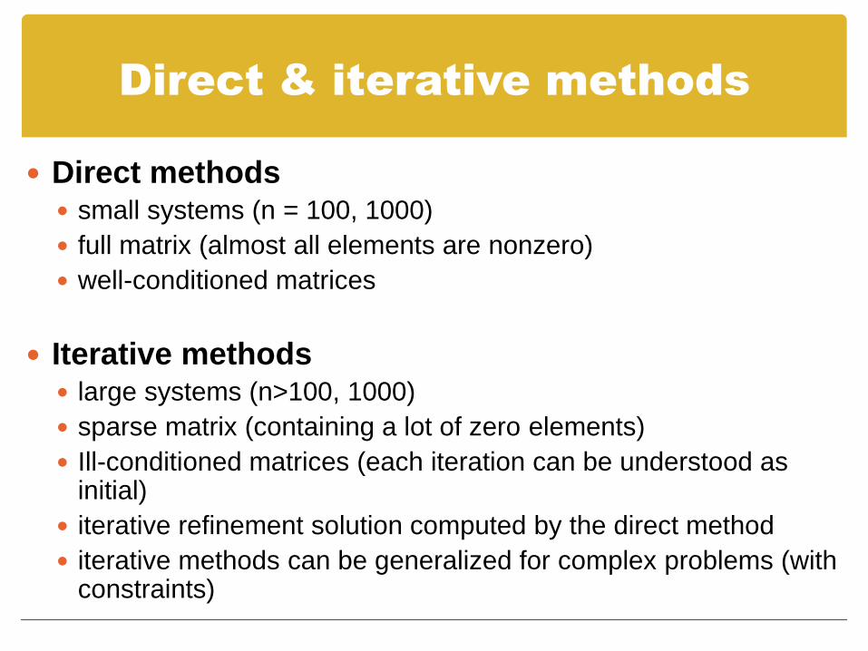
Direct & iterative methods
Direct methods small systems (n = 100, 1000)
full matrix (almost all elements are nonzero)
well-conditioned matrices
Iterative methods large systems (n>100, 1000)
sparse matrix (containing a lot of zero elements)
Ill-conditioned matrices (each iteration can be understood as initial)
iterative refinement solution computed by the direct method
iterative methods can be generalized for complex problems (with constraints)
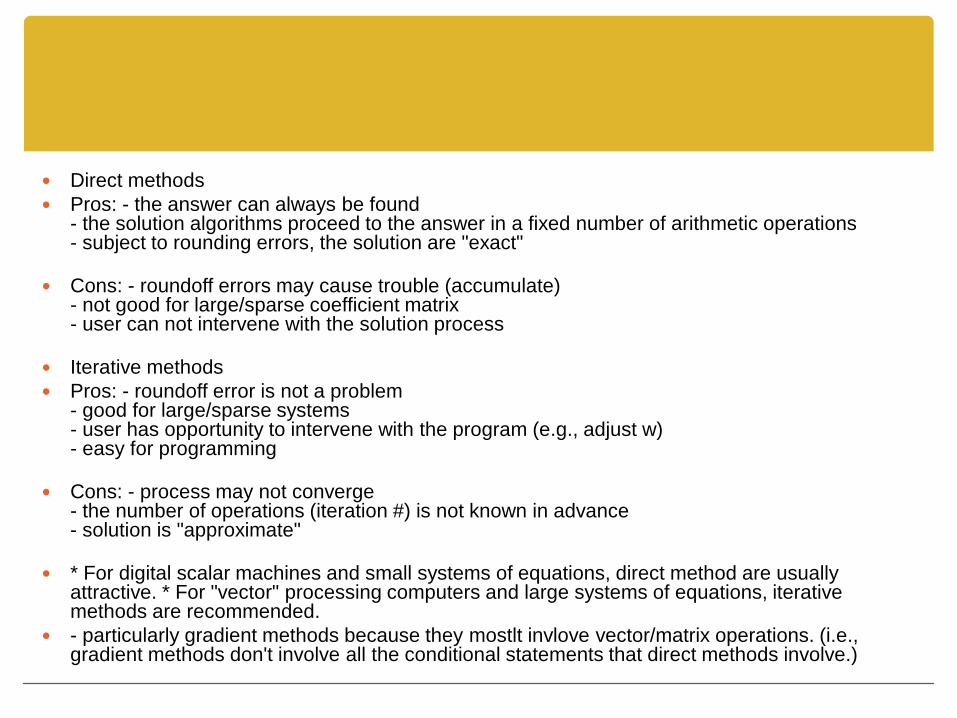
Direct methods
Pros: - the answer can always be found - the solution algorithms proceed to the answer in a fixed number of arithmetic operations - subject to rounding errors, the solution are "exact"
Cons: - roundoff errors may cause trouble (accumulate) - not good for large/sparse coefficient matrix - user can not intervene with the solution process
Iterative methods
Pros: - roundoff error is not a problem - good for large/sparse systems - user has opportunity to intervene with the program (e.g., adjust w) - easy for programming
Cons: - process may not converge - the number of operations (iteration #) is not known in advance - solution is "approximate"
* For digital scalar machines and small systems of equations, direct method are usually attractive. * For "vector" processing computers and large systems of equations, iterative methods are recommended.
- particularly gradient methods because they mostlt invlove vector/matrix operations. (i.e., gradient methods don't involve all the conditional statements that direct methods involve.)

General linear iterative method
The system Ax = b can be written in iterative form
x = Cx + d
Choice the initial approximation: x(0)
Computing of approximations x(k+1) :
x(k+1) = Cx(k) + d, k = 0, 1, 2, …
Stopping criterion: || x(k+1) - x(k) || ≤ ε,
where ε > 0 is a prescribed tolerance

Example 1
Iterative matrix
Recurrent formulas
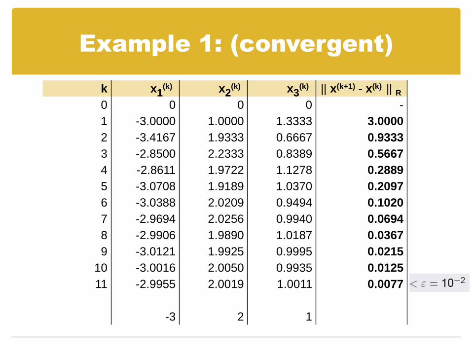
Example 1: (convergent)
k x1(k) x2
(k) x3(k) || x(k+1) - x(k) || R
0 0 0 0 -
1 -3.0000 1.0000 1.3333 3.0000
2 -3.4167 1.9333 0.6667 0.9333
3 -2.8500 2.2333 0.8389 0.5667
4 -2.8611 1.9722 1.1278 0.2889
5 -3.0708 1.9189 1.0370 0.2097
6 -3.0388 2.0209 0.9494 0.1020
7 -2.9694 2.0256 0.9940 0.0694
8 -2.9906 1.9890 1.0187 0.0367
9 -3.0121 1.9925 0.9995 0.0215
10 -3.0016 2.0050 0.9935 0.0125
11 -2.9955 2.0019 1.0011 0.0077
-3 2 1

Example 2 (divergent)
Iterative matrix
Recurrent formulas

Example 2 (divergent)
k x1(k) x2
(k) x3(k) || x(k+1) - x(k) || R
0 0 0 0 -
1 -12 5 -4 12
2 37 13 -13 49
3 -84 -108 -106 121
4 344 711 -236 819
5 139 -3291 -2003 4002
6 286 14894 -4864 18185
7 23752 -55279 -34640 70173
8 -57267 208257 -107037 263536
-3 2 1
divergent

Jacobi iterative method
Transformation to iterative form: we express x1 from eq. 1,
x2 from eq. 2, etc.
By equations:
Matrix form:

Gauss-Seidel iterative method
Jacobi method: (Example 1)
Gauss-Seidel method:
Goal: to improve the convergence

Gauss-Seidel iterative method
k x1(k) x2
(k) x3(k) || x(k+1) - x(k) || R
0 0 0 0 -
1 3.0000 -2.2000 -1.0667 3.0000
2 2.9833 -1.9800 -0.9989 0.2200
3 3.0044 -2.0020 -0.9992 0.0220
4 2.9991 -1.9998 -1.0002 0.0054
-3 2 1

Gauss-Seidel iterative method
By equations:
Matrix form:

Diagonally dominant matrix
DEFINITION:
a matrix is said to be strictly diagonally dominant if for
every row of the matrix, the magnitude of the diagonal entry
in a row is larger than to the sum of the magnitudes of all
the other (non-diagonal) entries in that row

Lemma
Lemma:
Jacobi (and also Gauss-Seidel) method
converges for every initial approximation x(0) if the
matrix of the system Ax = b is strictly diagonally
dominant.
Remark:
If the matrix is not strictly diagonally dominant we
can transform the system properly.

Example
Original system
Transformed system

Convergence
… next week

References
This presentation was prepared using the materials
by Radek Kučera:
NUMERICKÉ METODY (in Czech)
http://homel.vsb.cz/~kuc14/textyNM/kap4.pdf
http://homel.vsb.cz/~kuc14/textyNM/nm_pr05.pdf


