
Local Climate Zone Classification Using Random Forests
Ericka B. Smith
1 Introduction
1.1 Background
Urban Heat Islands, where urban areas are warmer than the neighboring rural areas, are a major
concern as the population worldwide increases and urbanizes (United Nations et al., 2019). This
is for four primary reasons: increased energy consumption, elevated emissions of air pollutants
and greenhouse gasses, compromised human health and comfort, and impaired water quality (US
EPA, 2014). They are caused because urban built structures hold more heat than the structures and
vegetation in surrounding areas (Hibbard et al., 2017). In particular, cities have an overabundance
of impervious surfaces, along with a lack of vegetation (Hibbard et al., 2017). Knowledge about
microclimates within cities, especially in the context of prospective sites for climate risk adaptation
efforts, has the potential to ease some of these disturbances (Lempert et al., 2018) .
Unfortunately, information on these sites can be difficult to obtain. Despite ample satellite imagery,
the current methods to classify this imagery are not always accurate (Yokoya et al., 2018). The
historic focus on broad categories of urban vs. rural does not give enough information about the
nuanced climate within a large urban area (Stewart & Oke, 2012). Local Climate Zone (LCZ)
classification was created by Stewart and Oke (2012) (Figure 1) to alleviate this problem, but it
often requires a significant investment from individuals with specialist knowledge to successfully
classify a city (Bechtel et al., 2015). Therefore, machine learning methods that can classify LCZ
1

efficiently and accurately are of great interest right now.
Figure 1: Local Climate Zone classes. Originally from Stewart and Oke (2012) and remade by Bechtel etal. (2017), licensed under CC-BY 4.0
1.2 Objective
The goal of this project is to recreate aspects of the article “Comparison between convolutional
neural networks and random forest for local climate zone classification in mega urban areas using
Landsat images” (Yoo et al., 2019), where methods for predicting LCZ classes for four large cities
throughout the world were compared. To do so, a small training dataset from the 2017 Institute of
Electrical and Electronics Engineers (IEEE) Geoscience and Remote Sensing Society (GRSS) Data
Fusion Contest (Tuia et al., 2017) was used as ground truth for LCZ classes. This was combined
with Landsat 8 satellite input data to create a series of models, which were then compared to a larger,
full LCZ layer for each city and assessed for accuracy. The primary types of models considered
2

in the Yoo et al. (2019) work were random forests and convolutional neural networks. However,
for this project the focus will be only on random forests. In addition, this investigation targets just
Hong Kong. This city was chosen because each LCZ that is classified has at least 4 polygons.
Finally, here, a classification scheme like the one used by the World Urban Database and Access
Portal Tools (WUDAPT) project, denoted as Scheme 1 in Yoo et al. (2019) will be the focus, with
comparisons between accuracy at different values of a tuning parameter.
All code and higher resolution images for this project can be found on GitHub at https://github.
com/erickabsmith/masters-project-lcz-classification.
2 Methods
2.1 Data
The LCZ reference data from the contest set was taken from the WUDAPT database, checked
for correctness, and then provided as a 100m resolution raster layer. The classes are numbered
1-17, rather than 1-10 and A-G, and I keep this structure throughout the analysis. The first step I
took was dividing the polygons of each class in this reference data into training and testing groups.
This required some preprocessing since the data did not have any sort of polygon identification, and
pixels within the same polygon should not be put into both training and validation groups because it
can artificially increase accuracy metrics (Zhen et al., 2013). The resulting groups are not exactly
equal in pixel numbers, but I determined that some aspect of randomization of polygons takes
precedence over equality in pixels due to this concern about accuracy metrics. In order to get as
close as possible a barplot was made showing the number of pixels in training and test, by class, so
3

that equality in pixel number could be explored without having knowledge of polygon groupings.
Sampling was repeated until these bars looked marginally even (Table 1).
Table 1: Delineation of training and test data by polygon and pixel.Local Climate Zone Train Test
Class 1: Compact high-rise 13 (295) 13 (336)Class 2: Compact mid-rise 6 (117) 5 (62)Class 3: Compact low-rise 7 (185) 7 (141)Class 4: Open high-rise 10 (275) 9 (398)Class 5: Open mid-rise 4 (79) 4 (47)Class 6: Open low-rise 6 (60) 7 (60)Class 7: Lightweight low-rise 0 (0) 0 (0)Class 8: Large low-rise 4 (90) 5 (47)Class 9: Sparsely built 0 (0) 0 (0)Class 10: Heavy Industry 4 (107) 5 (112)Class 11: Dense trees 7 (762) 7 (854)Class 12: Scattered trees 6 (194) 7 (213)Class 13: Bush, scrub 4 (459) 5 (232)Class 14: Low plants 6 (346) 6 (222)Class 15: Bare rock or paved 0 (0) 0 (0)Class 16: Bare soil or sand 0 (0) 0 (0)Class 17: Water 5 (1266) 5 (1113)a Number of polygons is listed first, with number of pixels in parentheses.
The Landsat 8 data I used includes four different dates, or “scenes,” each of whichwere downloaded
from the USGS EarthExplorer portal (Table 2). Then the atmospheric and panchromatic bands
were left out, and the data were resampled using the area weighted average to 100m x 100m grids
(Yokoya et al., 2018). I accessed these data from the IEEE GRSS Data Fusion Contest. This
slightly differs to Yoo et al. (2019) who collected their own Landsat data, but followed the same
processing steps. To get these data into a usable format I loaded the raster files into R by band and
then stacked with the LCZ reference data and converted to a dataframe, ready to be used as input
data. All 9 available bands of all 4 Landsat scenes amounted to 36 input variables. Each pixel is an
observation, with 279,312 pixels total over the almost 2,800 square kilometers that are contained
within the area of interest. The LCZ reference data has 179 polygons, which cover 8,846 pixels.
This is approximately 88.5 square kilometers and 3% of the total area of interest.
4

Table 2: Acquisition Dates of Each Landsat 8 SceneScene Date
1 29-Nov-20132 15-Oct-20143 16-Nov-20144 18-Oct-2015
2.2 Random Forests
Random forests consist of many decision trees. A decision tree can be used for classification or
regression, but here I will focus on classification since my goal is to predict LCZ class, a categorical
variable. Decision trees put each observation through a series of conditional statements, or splits,
in order to group it with other observations that are similar. The similar groups are expected to have
similar values for the predictor variable. Since the true value of the predictor variable is known for
the observations in the training dataset, it is possible to measure the accuracy of each prospective
split while building the tree.
Each point in which the data could potentially be split into two groups is called a node. Nodes
are selected such that each one uses the conditional statement which subsets the data into the best
possible split. When any more subsetting does not increase accuracy, the path ends, and this is
called a leaf node. The initial node is called the root node, and any nodes between the root node
and leaf nodes are called internal nodes. Splits are typically evaluated by Gini impurity or entropy.
Since I use the randomForest() function, which is within the randomForest package (Liaw &
Wiener, 2002) in R, I will describe everything in terms of its default, Gini impurity:
Gini Impurity = 𝐼𝐺(𝑡) = 1 −𝐶
∑𝑖=1
𝑝(𝑖|𝑡)2 (1)
Where 𝑖 is a class in the predictor variable, ranging from 1 to 𝐶; 𝐶 is the total number of classes;
5

and 𝑝(𝑖|𝑡) is the proportion of samples that belong to each 𝑖, for a particular node 𝑡.
A Gini Impurity of 0 indicates a completely homogeneous group, which cannot be improved upon.
This metric is used for comparison, where all possible variables and thresholds within those vari-
ables are tested. Then the variable and threshold with the best (lowest) value is selected for the node.
This is done recursively at each node until no split offers a decrease in the metric of choice. The
resulting collection of nodes is a decision tree. Decision trees perform poorly with new samples.
Including a threshold value for the accuracy metric can help, as it keeps trees more simple, but they
are still prone to overfitting. Collecting them into a random forest addresses this issue, in addition
to adding a component of randomness. The predictive aspect of a random forest is determined by
totaling up the decisions, or “votes,” that all the decision trees within the forest make.
Each tree is created individually and starts with bootstrapping the training dataset, with replace-
ment. This results in about 1/3 of the observations being excluded from each tree’s sample, called
the “out-of-bag” (OOB) data (Breiman, 2001). The observations included in the sample are “in-
bag.” These groupings allow for validation of the model without use of an external dataset. Then
the process is similar to the one described above for decision trees, except that, for each node only
a subset of the variables are randomly selected and used as candidates to split up the bootstrapped
data. This is advantageous due to both the randomness introduced and due to a reduction in corre-
lation. Whichever variable best splits the data will be the one kept at that node in that specific tree.
This is either done recursively until no more splits are beneficial (just as in a regular decision tree),
or until minimum size of the node is reached. To create the next tree the process is the same, but
with a new bootstrap sample. This is repeated for a chosen number of trees.
The choice of the number of trees to create is a tuning parameter. Too many trees can be computa-
6

tionally expensive, but too few can create a model that is poor at prediction. Tuning parameters are
usually adjusted based on OOB error rates, which is the overall proportion of incorrect predictions
based on the OOB data. It is calculated by putting each observation through each decision tree in
the random forest for which it is OOB. The predictions from each tree are then combined by direct
vote (for categorical variables) and this becomes the final predicted result for that observation. This
result is compared with the true value and counted as either correct or incorrect. This is repeated
for each observation in the dataset. In this analysis I use both OOB error and the metrics listed in
the Accuracy Assessment section for evaluation.
To use a random forest to make predictions for a new set of input values, the observations are fed
into each decision tree individually and the predictions are tallied up. Since there is not a known
ground truth value for each observation and each observation was not included in the creation of
the model, all trees are used. This overall process is called bagging, because it is the action of
bootstrapping the data to create each tree and using the aggregate to make a decision. Bagging is
useful because it reduces variance without introducing bias. For this analysis, the number of trees
parameter was varied individually. I chose it as parameter of interest because reducing it as much
as possible can have a large impact on time and computational resources required.
2.3 Accuracy Assessment
Following Yoo et al. (2019) and the remote sensing field, overall accuracy will be used as one
metric:
Overall Accuracy = 𝑂𝐴 = number of correctly classified reference sitestotal number of reference sites
(2)
7

𝑂𝐴urb and 𝑂𝐴nat will also be used, which are the same as OA but only include the urban or natural
classes, respectively. In addition, the F1 score will be used as a class level metric:
𝐹1 Score = 2 ∗ 𝑈𝐴 ∗ 𝑃𝐴𝑈𝐴 + 𝑃𝐴 (3)
where,𝑈𝐴(𝑧) = number of correctly identified pixels in class z
total number of pixels identified as class z(4)
𝑃𝐴(𝑧) = number of correctly identified pixels in class znumber of pixels truly in class z
(5)
UA is a measure of user’s accuracy, which is also called precision or positive predictive value.
PA is the measure of producer’s accuracy, also known as recall or sensitivity. The 𝐹1 score is the
harmonic mean of UA and PA. An 𝐹1 score closer to 1 indicates a model that has both low false
positives and low false negatives.
3 Results
3.1 Varying the Parameter for Number of Trees
The parameter for the number of trees was initially varied between 5 and 500 at intervals of 5. The
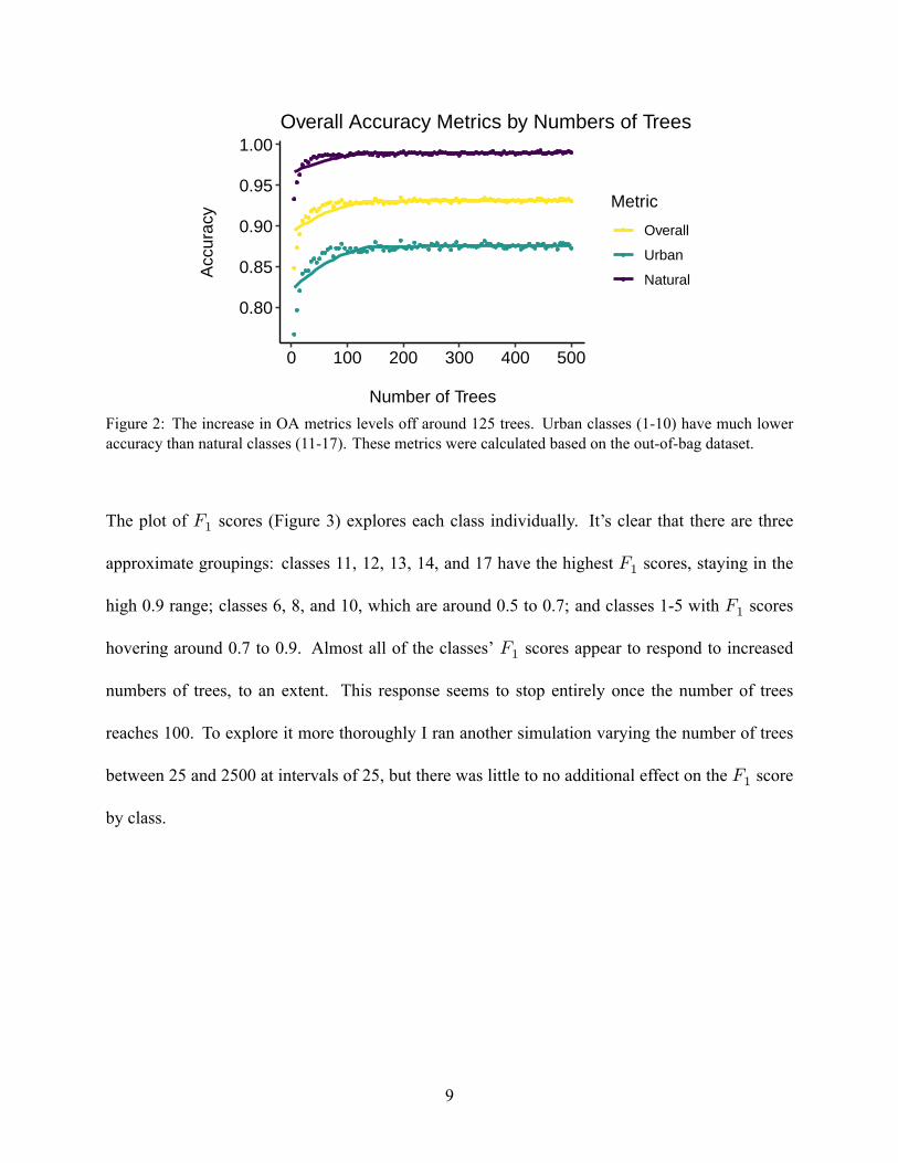
resulting overall accuracy metrics indicate a leveling off around 125 trees (Figure 2). There’s also a
clear distinction between accuracy in urban vs. natural classes, with natural classes having a much
higher overall accuracy.
8
0.80
0.85
0.90
0.95
1.00
0 100 200 300 400 500
Number of Trees
Acc
urac
y Metric
Overall
Urban
Natural
Overall Accuracy Metrics by Numbers of Trees
Figure 2: The increase in OA metrics levels off around 125 trees. Urban classes (1-10) have much loweraccuracy than natural classes (11-17). These metrics were calculated based on the out-of-bag dataset.
The plot of 𝐹1 scores (Figure 3) explores each class individually. It’s clear that there are three
approximate groupings: classes 11, 12, 13, 14, and 17 have the highest 𝐹1 scores, staying in the
high 0.9 range; classes 6, 8, and 10, which are around 0.5 to 0.7; and classes 1-5 with 𝐹1 scores
hovering around 0.7 to 0.9. Almost all of the classes’ 𝐹1 scores appear to respond to increased
numbers of trees, to an extent. This response seems to stop entirely once the number of trees
reaches 100. To explore it more thoroughly I ran another simulation varying the number of trees
between 25 and 2500 at intervals of 25, but there was little to no additional effect on the 𝐹1 score
by class.
9

Type
Natural
Urban
1
2
3
4
5
6
8
10
0 100 200 300 400 500
0.750.80
0.650.700.750.80
0.780.810.840.870.90
0.600.650.700.750.80
0.750.800.850.90
0.50.60.7
0.550.600.650.700.75
0.50.60.7
F−
1 S
core
11
12
13
14
17
0 100 200 300 400 500
0.96
0.97
0.98
0.75
0.80
0.85
0.90
0.8500.8750.9000.9250.9500.975
0.840.880.920.96
0.99600.99650.99700.99750.99800.9985
F−1 Score by Class for 5 to 500 Trees
Number of TreesFigure 3: The variation between LCZ classes in F-1 score can be seen. As the number of trees in the randomforest increases, F-1 score also increases, until around 100 trees. These metrics were calculated based on theout-of-bag dataset.
3.2 Predicting on the Test Dataset
3.2.1 Validation Metrics
OAand𝐹1 metrics dropped dramatically upon applying the random forest to the test data (Figure 4).
The 𝐹1 Score for class 17, Water, remained high, but since water has a very characteristic signature
this is not surprising (Xie et al., 2016). Classification for classes 2, 5, 8, and 14 performed especially
poorly.
10

Type Natural Overall Urban
OA−URB
OA
OA−NAT
0.00 0.25 0.50 0.75 1.00 0.00 0.25 0.50 0.75 1.00
F1−14
F1−13
F1−12
F1−11
F1−17
F1−5F1−2F1−8
F1−10F1−6F1−4F1−1F1−3
Validation Metrics for Test Dataset
Figure 4: Accuracy among random forest predictions for the test dataset varied widely, but was lower thanexpected for F-1 scores, which do not seem to to be consistent with the OA metrics. Classes 2, 5, 8, and 14have particularly low F-1 Scores
3.2.2 Importance Measures
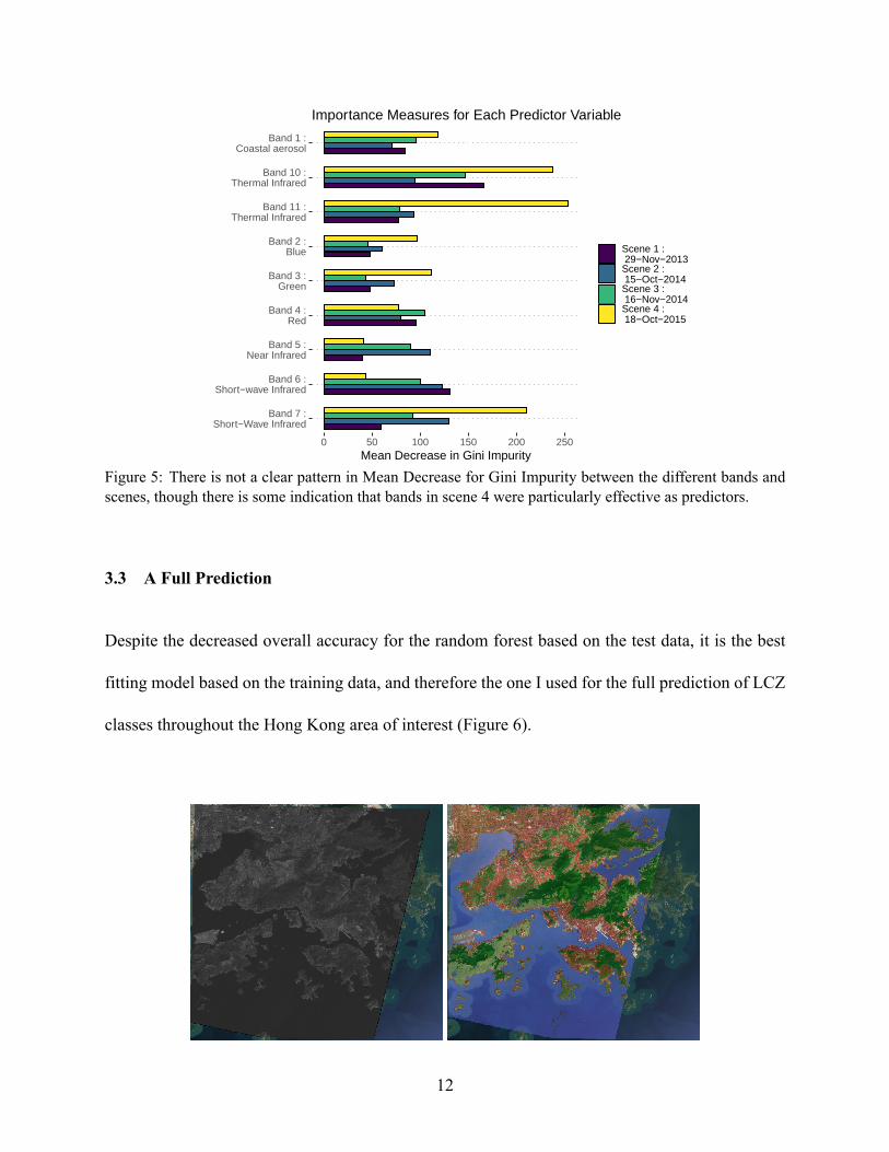
In general there is not a clear pattern in which bands or scenes proved to be the best predictors
based on mean decrease in Gini Impurity (Figure 5). However, bands 7, 10, and 11 in Scene 4
were particularly useful. Scene 4 overall seems to contribute the most effectively to the model,
surpassing the other scenes in all of the bands except for 4, 5, and 6.
11
0 50 100 150 200 250
Band 1 : Coastal aerosol
Band 10 : Thermal Infrared
Band 11 : Thermal Infrared
Band 2 : Blue
Band 3 : Green
Band 4 : Red
Band 5 : Near Infrared
Band 6 : Short−wave Infrared
Band 7 : Short−Wave Infrared
Mean Decrease in Gini Impurity
Scene 1 : 29−Nov−2013Scene 2 : 15−Oct−2014Scene 3 : 16−Nov−2014Scene 4 : 18−Oct−2015
Importance Measures for Each Predictor Variable
Figure 5: There is not a clear pattern in Mean Decrease for Gini Impurity between the different bands andscenes, though there is some indication that bands in scene 4 were particularly effective as predictors.
3.3 A Full Prediction
Despite the decreased overall accuracy for the random forest based on the test data, it is the best
fitting model based on the training data, and therefore the one I used for the full prediction of LCZ
classes throughout the Hong Kong area of interest (Figure 6).
12

1 : Compact Highrise
2 : Compact Midrise
3 : Compact Lowrise
4 : Open Highrise
5 : Open Midrise
6 : Open Lowrise
8 : Large lowrise
10 : Heavy industry
11 : Dense trees
12 : Scattered trees
13 : Bush or scrub
14 : Low plants
17 : Water
Figure 6: Imagery of the area of interest. Each has a basemap of satellite reference imagery. Top Left: OneLandsat 8 Scene with a map baselayer. Top Right: A fully predicted LCZmap with a map baselayer. Bottom:LCZ legend.
4 Discussion
The results of these analyses point to two primary issues in the current method for using random
forests to classify LCZ classes. The first is the large decrease in accuracy between prediction for the
OOB sample as compared to that of the test dataset. This is not necessarily surprising considering
the spatial autocorrelation inherently present in data like these, but it is concerning. OOB error is
often used to tune the model parameters and these results suggest that it causes overconfidence in
model success. Even when using the 𝑂𝐴 and 𝐹1 metrics on the OOB sample there were much
higher accuracy estimates than I saw with the test dataset. This points to a clear (though somewhat
impractical, considering data availability) solution, which is that there should be an independent
set of data used for building the model that is separate from both the testing and training data.
The second issue I observed is that use of an aggregate measure like 𝑂𝐴 can mask very low ac-
curacy in specific LCZ class categories, which were seen in the 𝐹1 by class scores. For example,
water has an accuracy of almost 100% by every metric tested. It also takes up a large proportion
of the training and test data, as well as the overall area of interest. As has been mentioned, the sig-
nature for water is quite distinctive (Xie et al., 2016). Therefore it is reasonable to suggest that the
13

high rate of correct predictions is not due to the suitability of random forest classification for LCZ
classes, but rather it may be due to the general ease of classifying water with Landsat 8 imagery,
despite method used. I don’t think this is unique to the Hong Kong area as it’s possible that any
dominant class could monopolize the predictions.
That being said, there are a number of other potential reasons this discrepancy in accuracy be-
tween classes and between OOB samples as compared to test data could be occurring. The uneven
distribution of polygons between different classes in the training dataset is likely an important con-
tributor. The small proportion of training and test pixels relative to the entire area of interest also
may be cause for concern. The latter is not tested for our accuracy methods due to lack of a fully
classified ground truth layer. Without this layer it is not possible to test the transferability of these
models to other urban areas, but based on the classification success within Hong Kong, it is likely
that transferability is poor.
In terms of my results varying the number of trees in the random forest, there is an upper limit
to how accurate the model can be. That upper limit may be in part due to the appropriateness
of the method, but I postulate that the quality and amount of data are the true culprits. This is a
limitation of my current analysis and I suggest it as an area for future study. It would be valuable to
understand what level of initial classification commitment is necessary for a robust LCZ analysis.
Another limitation is the use of only one tuning parameter. I expect further experimentation of
other important tuning parameters, as well as investigation of any interactions between them, may
point toward solutions that do not require more investment in initial classification.
14

5 References
• A. Liaw and M. Wiener (2002). Classification and Regression by randomForest. R News 2(3), 18–22.
• Bechtel, B., Alexander, P., Böhner, J., Ching, J., Conrad, O., Feddema, J., Mills, G., See, L., & Stewart, I.(2015). Mapping Local Climate Zones for a Worldwide Database of the Form and Function of Cities. ISPRSInternational Journal of Geo-Information, 4(1), 199–219. https://doi.org/10.3390/ijgi4010199
• Breiman, L. Random Forests. Machine Learning 45, 5–32 (2001). https://doi.org/10.1023/A:1010933404324
• Demuzere, Matthias; Hankey, Steve; Mills, Gerald; Zhang, Wenwen; Lu, Tianjun; Bechtel, Benjamin (2020):CONUS-wide LCZmap and TrainingAreas. figshare. Dataset. https://doi.org/10.6084/m9.figshare.11416950.v1
• Hibbard, K. A., Hoffman, F. M., Huntzinger, D., West, T. O., Wuebbles, D. J., Fahey, D. W., Hibbard, K.A., Dokken, D. J., Stewart, B. C., & Maycock, T. K. (2017). Ch. 10: Changes in Land Cover and TerrestrialBiogeochemistry. Climate Science Special Report: FourthNational ClimateAssessment, Volume I. U.S. GlobalChange Research Program. https://doi.org/10.7930/J0416V6X
• Lempert, R. J., Arnold, J. R., Pulwarty, R. S., Gordon, K., Greig, K., Hawkins-Hoffman, C., Sands, D.,& Werrell, C. (2018). Chapter 28: Adaptation Response. Impacts, Risks, and Adaptation in the UnitedStates: The Fourth National Climate Assessment, Volume II. U.S. Global Change Research Program.https://doi.org/10.7930/NCA4.2018.CH28
• Stewart, I. D., & Oke, T. R. (2012). Local Climate Zones for Urban Temperature Studies. Bulletin of theAmerican Meteorological Society, 93(12), 1879–1900. https://doi.org/10.1175/BAMS-D-11-00019.1
• Tuia, D., Moser, G., Le Saux, B., Bechtel, B., & See, L. (2017). 2017 IEEE GRSS Data Fusion Contest: OpenData for Global Multimodal Land Use Classification [Technical Committees]. IEEE Geoscience and RemoteSensing Magazine, 5(1), 70–73. https://doi.org/10.1109/MGRS.2016.2645380
• United Nations, Department of Economic and Social Affairs, & Population Division. (2019). World urbaniza-tion prospects: The 2018 revision.
• US EPA, O. (2014, June 17). Heat Island Impacts. US EPA. https://www.epa.gov/heatislands/heat-island-impacts
• Xie, H., Luo, X., Xu, X., Pan, H., & Tong, X. (2016). Evaluation of Landsat 8 OLI imagery forunsupervised inland water extraction. International Journal of Remote Sensing, 37(8), 1826–1844.https://doi.org/10.1080/01431161.2016.1168948
• Yokoya, N., Ghamisi, P., Xia, J., Sukhanov, S., Heremans, R., Tankoyeu, I., Bechtel, B., Saux, B. L., & Moser,G. (2018). Open Data for Global Multimodal Land Use Classification: Outcome of the 2017 IEEE GRSS DataFusion Contest. IEEE Journal of Selected Topics in Applied Earth Observations and Remote Sensing, 11(5),15.
• Yoo, C., Han, D., Im, J., & Bechtel, B. (2019). Comparison between convolutional neural networks and ran-dom forest for local climate zone classification in mega urban areas using Landsat images. ISPRS Journal ofPhotogrammetry and Remote Sensing, 157, 155–170. https://doi.org/10.1016/j.isprsjprs.2019.09.009
• Zhen, Z., Quackenbush, L. J., Stehman, S. V., & Zhang, L. (2013). Impact of training and vali-dation sample selection on classification accuracy and accuracy assessment when using referencepolygons in object-based classification. International Journal of Remote Sensing, 34(19), 6914–6930.https://doi.org/10.1080/01431161.2013.810822
15


