
Lower Oil Prices and the U.S. Economy:
Is This Time Different?
Christiane Baumeister and Lutz Kilian
October 2016 CEEPR WP 2016-014
A Joint Center of the Department of Economics, MIT Energy Initiative and MIT Sloan School of Management.

0
Lower Oil Prices and the U.S. Economy: Is This Time Different?*
November 14, 2016
Christiane Baumeister Lutz Kilian
University of Notre Dame University of Michigan CEPR CEPR
Abstract: We explore the effect on U.S. real GDP growth of the sharp and sustained decline in the global price of crude oil and hence in the U.S. price of gasoline after June 2014. Our analysis suggests that this decline produced a cumulative stimulus of about 0.9 percentage points of real GDP growth by raising private real consumption and non-oil related business investment and an additional stimulus of 0.04 percentage points reflecting a shrinking petroleum trade deficit. This stimulating effect, however, has been largely offset by a large reduction in real investment by the oil sector. Hence, the net stimulus since June 2014 has been close to zero. We show that the response of the U.S. economy was not fundamentally different from that observed after the oil price decline of 1986. Then as now the response of the U.S. economy is consistent with standard economic models of the transmission of oil price shocks. We found no evidence of an additional role for frictions in reallocating labor across sectors or for increased uncertainty about the price of gasoline in explaining the sluggish response of U.S. real GDP growth. Nor did we find evidence of financial contagion, of spillovers from oil-related investment to non-oil related investment, of an increase in household savings, or of households deleveraging. JEL codes: E32, Q43 Key Words: Stimulus; oil price decline; uncertainty; reallocation; savings; shale oil; oil loans. * This paper was prepared with financial support from the MIT Center for Energy and Environmental Policy Research, which we gratefully acknowledge. We thank Richard Curtin at the Institute for Social Research for providing access to additional data on gasoline price expectations in the Michigan Survey of Consumers that are not in the public domain. We also have benefited from helpful comments by David Chasman, Lucas Davis, Jim Hamilton, Ana Maria Herrera, Valerie Ramey, and Jim Stock. The paper was presented at the Brookings Papers on Economic Activity conference in Washington, DC, in September 2016.
Lutz Kilian, Department of Economics, 611 Tappan Street, University of Michigan, Ann Arbor, MI 48109-1220, USA. Email: [email protected]. Corresponding author: Christiane Baumeister, Department of Economics, 722 Flanner Hall, University of Notre Dame, Notre Dame, IN 46556, USA. Email: [email protected]
1
1. Introduction
Between June 2014 and March 2016, the real price of oil declined by 66%. There has been much
debate about the effect on U.S. growth of this sharp decline in global oil prices and hence in U.S.
gasoline prices. Many observers expected this oil price shock to boost the U.S. economy. Table 1
shows that, nevertheless, average U.S. real economic growth has increased only slightly since
2014Q2 from 1.8% to 2.2%. Breaking down the components of real GDP reveals a striking
discrepancy between sharply reduced average growth in real nonresidential investment, driven
by a dramatic fall in oil-related investment, and substantially higher average growth in real
private consumption. Moreover, real petroleum imports, which had been falling prior to 2014Q2,
have been rising again since 2014Q2, while the growth in real petroleum exports has nearly
doubled, reducing the petroleum trade deficit and adding to real GDP growth. The increase in
real petroleum exports is in contrast to the decline in overall real exports since 2014Q2.
The evidence in Table 1 raises a number of questions. Unexpected declines in the real
price of oil may affect the U.S. economy, for example, to the extent that they lower firms’ costs
of producing domestic goods and services. Why then did the decline in the real price of oil not
cause a strong economic expansion, as presumed in standard macroeconomic textbooks, which
interpret oil price shocks as shifts of the domestic aggregate supply curve (or, in a more modern
framework, as shifts in the cost of producing domestic real output)? Unexpected declines in the
real price of oil also matter for the economy, because they increase the demand for other
domestic goods and services, as consumers spend less of their income on motor fuels. One
question of interest thus is by how much we would have expected private real consumption to
increase as a result of the windfall income gain caused by lower oil prices. Did the actual growth
in private real consumption match expected growth or was it perhaps held back because the

2
decline in the global price of crude oil was not fully passed on to retail fuel prices? Or did
consumers simply choose not to spend their income gains, but to pay off their debts or increase
their savings instead? Finally, why did the real consumption of motor vehicles decline, despite an
overall increase in private real consumption? Were consumers perhaps reluctant to buy new
automobiles because of increased uncertainty about future gasoline prices, holding back overall
economic growth?
Another puzzle is why growth in private nonresidential investment declined as much as it
did after 2014Q2. Clearly, the answer is related to the increased importance of U.S. shale oil
production, raising the question of whether the growth of the shale oil sector has changed the
transmission of oil price shocks to the U.S. economy. The decline in oil-related investment in
response to falling oil prices not only has a direct effect on U.S. real GDP, but there are also
broader implications to consider. One concern has been that the decline of the shale oil sector
may have slowed growth across oil-producing states, dragging down aggregate U.S. growth.
Another conjecture has been that lower investment by oil producers may have slowed growth in
other sectors of the economy nationwide, as the demand for structures and equipment used in oil
production declined. A third conjecture has been that risky loans to oil companies may have
undermined the stability of the banking system, disrupting financial intermediation. A related
concern has been that the sustained decline in the real price of oil after 2014Q2 may have caused
an economic slowdown by leaving assets and oil workers stranded in a sector that is no longer
competitive.
Equally surprising is the evolution of the petroleum trade balance since 2014Q2, which
does not conform to the conventional wisdom that an unexpected decline in the price of oil is
associated with rising petroleum trade deficits, as domestic oil production declines. Finally, the

3
substantial decline in U.S. real non-petroleum exports is a reminder that the decline in the real
price of oil itself was associated at least in part with a global economic slowdown that in turn has
to be taken into account in explaining the comparatively slow U.S. economic growth.
In this paper, we investigate the empirical support for each of these conjectures. We
examine the channels by which the 2014-16 oil price decline might have affected the U.S.
economy and assess their quantitative importance, drawing on a wide range of macroeconomic,
financial and survey data, both at the aggregate level and at the sectoral and state level. Our
objective is to quantify how much of the evidence in Table 1 can be explained by the unexpected
decline in the real price of oil, without ruling out that other economic shocks may have affected
U.S. economic growth at the same time. In section 2, we provide evidence for the view that the
demand channel of the transmission of oil price shocks to the U.S. economy is more important
than the supply (or cost) channel emphasized in many theoretical models of the transmission of
oil price shocks, motivating our emphasis on the demand channel of transmission throughout the
remainder of this paper.
Our discussion of the demand channel focuses in particular on understanding the
evolution of private consumption, of investment spending, and of the petroleum trade balance. In
section 3, we examine to what extent standard economic models of the transmission of oil price
shocks that focus on changes in consumers’ discretionary income, as the decline in oil prices is
passed through to retail fuel prices, can explain the growth in real private consumption in Table 1
(see Edelstein and Kilian 2009; Hamilton 2009, 2013; Kilian 2014). In these models, a drop in
the real retail price of gasoline is akin to a tax cut from the point of view of consumers, which is
expected to stimulate private consumption and hence real GDP. The reasoning is analogous to
the conventional analysis of an unexpected increase in the real prices of oil and gasoline. In the
4
words of Yellen (2011):
“… higher oil prices lower American income overall because the United States is a major oil importer and hence much of the proceeds are transferred abroad. […] Thus, an increase in the price of oil acts like a tax on U.S. households, and … tends to have a dampening effect on consumer spending. […] Staff analysis at the Federal Reserve Board indicates that a dollar increase in retail gasoline prices … reduces household disposable income ... and exerts a significant drag on consumer spending.”
Yellen goes on to stress that the effect of these shocks on the economy has changed, as
households’ dependence on gasoline has evolved over time. Underlying this analysis is the view
that oil price shocks represent terms-of-trade shocks that affect domestic spending and, hence,
real GDP growth through a Keynesian multiplier. Although some of the so-called oil tax that is
transferred abroad may ultimately be recycled, as oil-exporting countries directly or indirectly
increase imports of U.S.-produced goods and services, this petrodollar recycling tends to occur
with a considerable delay, if at all.1
In response to an unexpected fall in the price of oil, as occurred after June 2014, the basic
mechanism described by Yellen operates in reverse, and is expected to generate a stimulus for
the U.S. economy. We quantify this effect based on estimates of a linear regression model of the
relationship between changes in real U.S. private consumption and changes in consumers’
purchasing power associated with gasoline price fluctuations, controlling for the evolution of the
share of fuel expenditures in total consumer expenditures. Estimates of this baseline model
suggest that unexpectedly low oil prices cumulatively raised average U.S. real GDP growth after
2014Q2 by about 0.7 percent, as purchasing power increased and private consumption expanded.
1 As discussed in Hamilton (2013), an exogenous increase in the real price of price of oil may have real effects even in a closed economy. Given that the price elasticity of gasoline demand is comparatively low, an exogenous increase in the price of gasoline causes a reduction in consumers’ discretionary income. Although in a closed economy consumers’ increased spending on gasoline represents income for someone else by construction, it may take considerable time for this income to be returned to consumers in the form of company profits, royalties, or dividends paid to shareholders, or to be spent by oil companies in the form of increased investment expenditures. Differences in the marginal propensity to spend thus may affect the overall level of spending and hence the business cycle in the short run.

5
We show similar estimates are also obtained after incorporating a measure of changes in the
dependence of the U.S. economy on crude oil imports and gasoline imports in the construction of
the purchasing power shocks.
In section 4, we examine an alternative view in the literature, according to which the
conventional linear model is overstating the stimulus for real GDP growth, because the true
relationship between the price of oil and the economy is governed by a time-invariant, but
nonlinear process. Proponents of this view point to a number of indirect channels of transmission
ignored by the baseline model. For example, it could be argued that the stimulating effects of the
oil price decline discussed earlier are offset by delays in the reallocation of resources (see
Hamilton 1988; Bresnahan and Ramey 1993; Davis and Haltiwanger 2001; Ramey and Vine
2011; Herrera and Karaki 2015; Herrera, Karaki, and Rangaraju 2016) or by higher oil price
uncertainty (see Bernanke 1983; Pindyck 1991; Elder and Serletis 2010; Jo 2014). Either of these
economic mechanisms would generate a nonlinearity that could explain why unexpected real oil
price increases are recessionary, yet unexpected real oil price declines may not be followed by
economic expansions and may even be recessionary. In section 4, we provide aggregate and
disaggregate evidence that suggests that neither of these interpretations fits the recent episode.
Building on the results in sections 3 and 4, in section 5, we quantify the extent to which
unexpectedly low oil and gasoline prices have stimulated private nonresidential investment
(excluding the oil sector). We make the case that this stimulus can be estimated from a linear
regression model similar to the model we employed for private consumption. This investment
stimulus adds another 0.2 percentage points of cumulative real GDP growth to the consumption
stimulus of 0.7 percentage points.
A common view is that the relationship between the economy and changes in the price of
6
oil has evolved in recent years, calling into question estimates of the stimulus based on linear
regression models. Proponents of this view would argue that this latest episode of declining oil
prices is fundamentally different from previous episodes of sustained declines in the price of oil
such as the 1986 episode, so nothing about the response of the economy can be learned from
fitting regressions to historical data. One candidate explanation for such a structural shift in
recent years is the increased importance of the U.S. shale oil sector since late 2008, which
created potentially important additional effects of oil price shocks on domestic value added, on
aggregate nonresidential investment expenditures, on the petroleum trade balance, and on the
stability of the banking sector. Likewise, a structural shift could arise if consumers used the
windfall income associated with lower oil prices to reduce their mortgage debt and credit card
debt rather than spending the extra income as in years past. In section 6, we examine the
empirical evidence for these and other hypotheses. We find no evidence that households’ savings
behavior has changed or that households have been deleveraging, but we find evidence of an
unprecedented decline in oil investment in the U.S. economy and of a systematic reduction in net
petroleum imports. The latter two structural shifts complicate the assessment of the response of
the U.S. economy to the recent decline in the price of oil.
A simple national income accounting calculation in section 7 suggests that the
stimulating effect of lower oil prices on private real consumption, on non-oil related
nonresidential investment, and on net petroleum exports after June 2014 was approximately
offset by the reduction in real investment by the U.S. oil sector. The net stimulus raised average
real GDP growth by a paltry 0.2% at annual rates. Finally, in section 8, we compare the response
of the economy to the decline in the price of oil after June 2014 to its response to the 1986 oil
price decline, and make the case that there are more similarities than differences. The most

7
important difference is that the recent decline in the real price of oil was about twice as large as
the decline in 1986, causing a sharper contraction in oil investment than in 1986. Moreover,
unlike the 1986 oil price decline, it was associated in part with a global economic slowdown,
reflected in a substantial decline in the growth of U.S. real non-petroleum exports, without which
average U.S. real GDP growth is likely to have reached 2.5% at annual rates after 2014Q2. The
concluding remarks are in section 9.
2. How Important is the Cost Channel of the Transmission of Oil Price Shocks?
The traditional undergraduate textbook analysis of the effects of oil price shocks on oil-
importing countries equates lower oil prices with a reduction in the cost of producing domestic
goods and services (and hence a shift in the domestic aggregate supply curve along the domestic
aggregate demand curve in the traditional undergraduate textbook model). This view has merit to
the extent that firms directly or indirectly rely on oil (or oil-based products) as a major factor of
production. Examples of such industries include the transportation sector, some chemical
companies, and rubber and plastics producers. For most industries, however, this channel is not
likely to be important. In fact, a large share of the oil used by the U.S. economy is consumed by
final consumers rather than by firms, which explains why more recent studies have typically
interpreted oil price shocks as affecting the disposable income of consumers. This more
contemporary view implies that oil price shocks are primarily spending or demand shocks for the
U.S. economy. Within the traditional undergraduate textbook model, they can be thought of as
shifts in the aggregate demand curve along the aggregate supply curve.
Some informal evidence regarding the relative importance of the supply (or cost) channel
of the transmission of oil price shocks and the demand channel of transmission may be obtained
by examining which sectors benefited and which suffered after the oil price decline. For
8
example, there is general agreement that the sector most sensitive to changes in fuel prices is
transportation. The data provide at best partial support for this view. Figure 1 shows that the
volume of truck tonnage evolved largely along the same trend before and after June 2014. In
contrast, airline passenger traffic accelerated, but only with a delay of half a year that is likely to
reflect the fact that airlines had hedged against higher oil prices in futures markets and were able
to pass on these added costs to the retail customer, when the price of oil fell. Rail freight traffic
initially remained relatively stable, but fell starting in early 2015, reflecting the global economic
slowdown in general and a substantial decline in U.S. coal shipments in particular. To a lesser
extent this pattern is also found in barge traffic and air freight traffic. A much smaller decline in
rail passenger traffic, in contrast, is likely to reflect substitution away from trains and toward
automobiles. Overall, these effects appear modest at best and are at odds with the view that lower
fuel costs have a large effect on real output in the transportation sector.
This conclusion is corroborated by data on the excess stock returns for selected sectors
and individual firms relative to the overall stock market index between July 2014 and March
2016.2 All results are expressed as average excess returns at annual rates. In general, companies
that cater to U.S. consumers tend to appreciate in value more than the average company. In
particular, candy and soda (+7%), beer and liquor (+10%), and tobacco (+16%) do well, perhaps
because such goods are sold at gas stations, but also food products (+7%), and apparel (+11%).
Both tourism (+11%) and restaurants, hotels and motels (+8%) benefited from lower oil prices,
as consumer demand rose. So did retail sales (+14%). Amazon (+38%) and Home Depot (+32%)
did particularly well. Only recreation, entertainment services, and publishing did not partake in
this boom.
2 The analysis is based on individual returns from Bloomberg and value-weighted industry-level stock returns from http://mba.tuck.dartmouth.edu/pages/faculty/ken.french/data_library.html. The benchmark portfolio is the value-weighted S&P500 stock return from Bloomberg.

9
The petroleum and natural gas sector (-28%), unsurprisingly, was hit hard. Within that
sector, refining companies that use crude oil as a production input fared somewhat better. Other
industries that rely on oil as a major input and hence would have been expected to profit from
lower oil prices such as rubber and plastics (+4%) and logistics (+2%) did not benefit much, and
chemicals (-6%) actually performed worse than the overall market, arguing against an important
supply (or cost) channel of transmission. Airlines (+15%) benefited both from lower fuel costs
and higher travel demand. Likewise, textiles were helped by lower input costs and higher
demand (+13%). The surprising fact that auto companies performed below average (-9%) is
largely explained by weak foreign sales, reflecting the recent global economic slowdown.
Sectors tied to commodity markets such as agriculture (-12%) or mining (-31%) performed
poorly for the same reason. Steel (-26%), fabricated metal products (-51%), machinery (-19%),
and ship building and railroad equipment (-13%), all suffered from lower demand, mainly due to
the decrease in global real economic activity.
We conclude that the supply (or cost) channel of the transmission of oil price shocks to
the U.S. economy, which is emphasized in many theoretical models of the transmission of oil
price shocks developed in the 1980s and 1990s, may be safely neglected. Lower fuel costs do not
appear to provide much of a stimulus to firms that are oil-intensive in production. The few
sectors other than refining that are heavily dependent on oil inputs performed only marginally
better than the rest of the economy after June 2014, if at all. In contrast, sectors sensitive to
fluctuations in consumer demand did far better than average, lending support to the conventional
view among policymakers and oil economists that the demand channel of the transmission of oil
price shocks to the U.S. economy is more important than the supply (or cost) channel (see Kilian
2014). Our industry-level analysis of excess stock returns provides strong evidence of a stimulus

10
to U.S. consumer demand, but also of lower demand from a global economic slowdown,
corroborating related results in the more recent literature including the narrative evidence in Lee
and Ni (2002) and the regression evidence in Kilian and Park (2009).
3. How Much Did the Unexpected Decline in the Price of Oil Stimulate Consumption?
Given the evidence in section 2, we focus on the demand channel of transmission. We first
examine private consumer spending, which accounted for 69% of U.S. GDP in 2014. For the oil
price decline after 2014Q2 to have stimulated U.S. private consumption, it is necessary for this
decline to have been passed through to retail fuel prices. We therefore first quantify the extent to
which U.S. gasoline prices have declined in response to lower crude oil prices, taking account of
the cost share of crude oil in producing gasoline. The answer to this question is not obvious
because there is a long-standing view that oil price declines are not necessarily passed on to retail
gasoline prices as quickly as oil price increases (see Venditti 2013). We provide evidence that
the pass-through is symmetric and that the recent oil price decline has been fully passed on to
retail gasoline prices. We then quantify the changes in U.S. consumers’ purchasing power
associated with unexpected changes in the price of gasoline and estimate the cumulative effect of
these shocks on real private consumption, controlling for changes in the share of gasoline
expenditures in total consumer expenditures. The magnitude of the estimated stimulus is shown
to be consistent with a back-of-the-envelope calculation that treats the change in the gasoline
price as taking place all else equal and takes account of the price elasticity of gasoline demand.
3.1. Has the Decline in the Oil Price after June 2014 Been Passed Through to Gas Prices?
Figure 2 shows the price of gasoline at the pump and the cost of the crude oil used in producing
gasoline. The difference between these time series reflects the evolution of gasoline taxes and the

11
costs of refining the crude oil and of marketing and distributing the gasoline.3 Figure 3 zooms in
on events since June 2014. All data are expressed as index numbers normalized to equal 100 in
June 2014. Between June 2014 and December 2015, the price of gasoline fell by 45%, whereas
the cost of crude oil fell by 65% (about as much as the spot price of Brent crude oil). Some of
that difference is accounted for by a slight increase in gasoline taxes, but even the pre-tax price
of gasoline fell only by 53%. At first sight this evidence might seem to imply that refiners and/or
gasoline distributors failed to pass on the full cost savings resulting from the 2014/15 oil price
decline to consumers. It is important to keep in mind, however, that historically only about half
of the price of gasoline has consisted of the cost of crude, so even under perfect pass-through one
would expect a percent decline in the price of gasoline only about half as large as the percent
decline in the cost of oil.
Table 2 examines the extent to which cumulative changes in the cost of the crude oil used
in producing gasoline have been reflected in changes in the price of gasoline based on four key
episodes, two of which involve increases in the cost of crude oil and two of which involve
declines. For example, between January 2007 and July 2008, the cost of crude oil increased
cumulatively by 155% (slightly more than the price of Brent crude oil). Given an average cost
share of 63.3% over this period, all else equal, one would have expected the price of gasoline to
increase by 98.1% cumulatively. The actual cumulative increase of 81.3% was somewhat lower,
but not far from this benchmark. Another large cumulative increase in the cost of oil occurred
between December 2008 and April 2011. The cost of oil surged by 175.4% (somewhat less than
3 Although there is a large degree of comovement between the cost of oil and the price of gasoline, this comovement is by no means perfect. For example, in 2005, when Gulf Coast oil refiners were forced to shut down due to Hurricanes Rita and Katrina, causing a refining shortage, there was a sharp spike in the price of gasoline, but not in the price of crude oil, illustrating that occasionally changes in gasoline prices are not just determined by changes in the price of crude oil (see Kilian 2010). A regression of the price of retail gasoline on an intercept and the cost of crude oil, as shown in Figure 2, yields a slope coefficient of 1.1, suggesting a near one-for-one relationship in the long run.

12
the Brent price of crude oil). Given the average cost share of 64.6%, one would have expected
the price of gasoline, all else equal, to increase by 113.3%. The actual increase of 125.3% was
somewhat higher, but in the same ballpark.
What about declines in the cost of crude oil? Between July 2008 and December 2008 the
cost of crude fell by 69.2% cumulatively, which, given the average cost share of 65.2%, would
have led us to expect the gasoline price to decline by 45.1%, somewhat less than the observed
decline of 58.5%. Likewise, the cumulative decline in the cost of oil of 65% between June 2014
and March 2016, given the average cost share of 51.4%, translates to an expected decline of 35%
in the U.S. gasoline price, compared with a somewhat larger decline of 46.7% in the data.
These four examples are consistent with the view that on average the observed changes in
gasoline prices are roughly as large as one would have expected under perfect pass-through,
given that gasoline prices may vary for a range of other reasons ranging from refinery outages to
changes in retail market structure (see Baumeister, Kilian and Lee 2016). The decline in the
price of gasoline that occurred in 2014/15, if anything, exceeded what one would have expected
based on the pass-through from the cost of oil to the gasoline price at the pump. There is no
evidence of asymmetries in the pass-through between declines and increases in the cost of oil in
Table 2, corroborating formal econometric results based on monthly data in Venditti (2013) that
did not control for changes in the cost share of oil.
3.2. How Has the Consumption of Gasoline Evolved Since June 2014?
Lower gasoline prices increase the discretionary income of consumers to the extent that the same
amount of gasoline may be purchased with less income. Lower gasoline prices, however, also
provide an incentive to increase gasoline consumption that reduces the extra income available for
other purchases. Figure 4 shows the evolution of seasonally adjusted U.S. gasoline consumption,
13
defined as the sum of the motor gasoline consumed by the industrial, commercial and
transportation sectors, since June 2014. Gasoline consumption cumulatively increased by 5.5%
between June 2014 and January 2015, reaching 7.4% by March 2016. The increase in gasoline
consumption coincided with a 5% increase in vehicle miles traveled since June 2014 (see Figure
5). At the same time, the fuel economy of new cars and light trucks, as measured by the average
sales-weighted miles per gallon reported by the Transportation Research Institute at the
University of Michigan, fell by 2% from a peak of 25.8 mpg in August 2014 to 25.2 mpg in
March 2016, reflecting changes in the composition of new vehicles.
3.3. Measuring Gasoline Price Shocks
Gasoline price shocks are defined as the difference between what the price of gasoline was
expected to be ex ante and what it actually turned out to be. Recent work by Baumeister and
Kilian (2016a) suggests that what matters when quantifying gasoline price shocks is the
expectation of the decision maker whose behavior we seek to understand. If we want to
understand the response of U.S. consumers, for example, the relevant measure of gasoline price
expectations is consumers’ own expectations, no matter how inaccurate that measure may be by
statistical criteria. The Michigan Survey of Consumers provides data starting in February 2006
for consumers’ expectations of the change in gasoline prices over the next 12 months. Based on
these data, Anderson, Kellogg and Sallee (2013) document that consumers with rare exceptions
expect the nominal price of gasoline to grow at the expected rate of inflation. An obvious
question is whether this approximation remains valid even during a decline in the price of
gasoline as sustained as the decline that started in June 2014.
We address this question in Figure 6, which plots the expectation of the price of gasoline
implied by the survey data. The gasoline price expectation is constructed by adding the median

14
expected change in gasoline prices over the next 12 months from the Michigan Survey of
Consumers to the average U.S. price of gasoline from the Monthly Energy Review. Figure 6
shows that this survey measure closely tracks the no-change forecast of the real price of gasoline
adjusted for the median expected change in the price level over the next 12 months, as reported
in the Michigan Survey of Consumers, even after June 2014. This evidence suggests that one can
approximate consumers’ expectations of the real gasoline price based on a simple no-change
forecast of the real price of gasoline. We employ this approach to construct a monthly time series
of the real gasoline price shocks experienced by U.S. consumers during 1970.1-2016.3.
Let 1 1( ) ( ) ,gas gas gast t t t t tS R E R E R where gas
tR is the real price of gasoline, defined as
the average nominal price of gasoline and other motor fuel, ,gastP as reported by the BEA,
deflated by the overall PCE deflator, ,CtP and 1 1( ) .gas gas
t t tE R R This shock measure simply
corresponds to the percent change in the real price of gasoline and other motor fuel, as shown in
the upper panel of Figure 7. How much this gasoline price shock matters to U.S. consumers
depends on the share of expenditures on gasoline and other motor fuels in overall consumer
expenditures. For a given unexpected increase in the real price of gasoline, the higher this
expenditure share, the higher the potential reduction in consumers’ discretionary income because
income spent on gasoline cannot be spent on other goods and services. As illustrated in the
middle panel of Figure 7, this share has fluctuated between about 2% and 5% since 1970. In mid-
1973, in early 2006, and again in mid-2014 the share was near its long-run average value of 3%.
A measure of the shock to consumers’ purchasing power may be constructed as
,gas gast t
t t ct t
C PPP S
C P
where gastC is real U.S. gasoline consumption and tC is real total consumption, as reported by
15
the BEA. The series of purchasing power shocks, ,tPP is shown in the bottom panel of Figure 7.
It is the latter shock series that consumers respond to rather than the gasoline price shock in the
upper panel. Figure 7 shows clear evidence of an unexpected increase in purchasing power in
1986, following a sharp drop in the global price of crude oil; it shows repeated unexpected
reductions in purchasing power between 1999 and 2008 during the surge in global oil prices; a
large positive purchasing power shock in late 2008, associated with the financial crisis, that was
quickly reversed in early 2009; and, finally, a series of positive and negative purchasing power
shocks since June 2014, during the period of interest in this paper.
3.4. The Baseline Linear Model
The question of ultimate interest is by how much these purchasing power shocks stimulated real
private consumption. Our analysis is based on a monthly model that embodies the identifying
assumption that changes in purchasing power are predetermined with respect to real
consumption.4 Let tc denote the percent change in monthly real consumption (demeaned to
account for the drop in average consumption growth from 3.3% at annual rates to 2.1% after
December 2008), and let tPP denote the monthly shock to consumers’ purchasing power, as
defined in section 3.3. The shocks are normalized such that a positive shock indicates an increase
in purchasing power. Then the response of consumption to purchasing power shocks may be
estimated from the OLS regression
6 6
1 0
,t i t i i t i ti i
c c PP u
(1)
where tu denotes the regression error.5 Given that there has been considerable variation in the
4 For related approaches see, e.g., Edelstein and Kilian (2009) and Hamilton (2009). The validity of this identifying assumption is supported by evidence in Kilian and Vega (2011). 5 The lag order choice follows Edelstein and Kilian (2009). The estimation sample is 1970.2 -2016.3.

16
magnitude and sign of the changes in purchasing power since June 2014, a more useful approach
to studying the evolution of U.S. real private consumption over this period is to compute the
cumulative effect of these purchasing power gains and losses on real consumption since June
2014. Table 3 shows that, according to the model, purchasing power shocks cumulatively
stimulated U.S. real private consumption by 1.2% and account for most of the observed 1.3%
cumulative increase in total real private consumption relative to trend between 2014.7 and
2016.3. Taking account of the drift, the model predicts an average growth rate of 2.8% at annual
rates in real private consumption, compared with 2.9% in Table 1.
Part of the estimated cumulative increase in consumption is accounted for by the
operating cost effect, which refers to an increase in purchases of automobiles in response to
unexpectedly lower gasoline prices, which amplifies the overall consumption response over and
above the discretionary income effect (see Hamilton 1988). Table 3 confirms the existence of a
disproportionately larger stimulus of near 3% for durables (which in turn is largely driven by the
consumption of new motor vehicles). Weighting the 6.7% stimulus for the consumption of new
motor vehicles in Table 3 by the share of new motor vehicles in private consumption of 2.3%
suggests a cumulative operating cost effect of 0.15%. Given the overall cumulative consumption
response of 1.2% in the baseline model, this implies a discretionary income effect of about
1.05%.6
A simple back-of-the-envelope calculation suggests that the magnitude of this estimate of
the discretionary income effect is reasonable. The real price of gasoline and other motor fuels
6 Ramey and Vine (2011) propose scaling the nominal gasoline price in 1973.12-1974.5 and in 1979.5-1979.7 by a multiplicative factor intended to capture the waiting cost at gas stations associated with government-imposed gasoline price ceilings. Because the waiting cost is not associated with a transfer of income abroad, this adjustment must not be used in quantifying the discretionary income effect. It may affect the operating cost effect, however. Further sensitivity analysis shows that adjusting tPP for the waiting cost only affects the third decimal place of our
estimates of the operating cost, so the waiting-cost adjustment may be safely ignored.

17
declined by 44.94% between June 2014 and March 2016. The share of gasoline expenditures in
total expenditures in June 2014 was 3.17%. This allows consumers to purchase the same goods
for a fraction of their income
(1 0.0317) 1 0.0317 (1 0.4494)(1 0.37 0.4494) 0.9887 ,
freeing up 1.13% of their income for additional purchases, after taking account of the increase in
gasoline consumption implied by the point estimate of -0.37 of the price elasticity of gasoline
demand reported in Coglianese et al. (2016). This exercise suggests a discretionary income effect
on consumption close to the estimate of 1.05% implied by the baseline model.
3.5. An Alternative Linear Specification
The regression model (1) is designed to capture the extent to which discretionary income is
injected into the U.S. economy or removed from the U.S. economy, as the terms of trade vary in
response to oil price shocks. This model implicitly assumes that the share of the proceeds from
gasoline that goes abroad is the same over time. To the extent that this share varies over time, the
model provides only an approximation. It may seem that variation in the dependence of the U.S.
economy on oil and gasoline imports over time would render this approximation inaccurate.
Assessing the empirical content of this concern is not straightforward. For example, it
may be tempting to answer this question by testing for structural breaks in the parameters of
model (1), but that approach would not be informative. It is well documented that mechanical
applications of tests for structural stability on subsamples are prone to generating spurious
rejections of the null hypothesis of a stable relationship between macroeconomic aggregates and
oil or gasoline prices (see, e.g., Kilian 2009, Kilian and Park 2009). Although the average
responses of real consumption to purchasing power shocks may be estimated reliably using long
enough samples, when considering short subsamples, these responses will change in magnitude

18
and even in sign, as the composition of oil demand and oil supply shocks evolves over time,
giving the mistaken appearance of structural instability, even when there is no structural change
at all. Spurious evidence of structural breaks arises, whenever oil price fluctuations over a
subsample are not representative of the full sample.
An alternative and more direct way of quantifying the importance of changes in the
dependence of the U.S. economy on oil and gasoline imports is to incorporate this evolution in
the construction of .tPP A simple approximation is to weight U.S. consumer expenditures on
gasoline by the share of the proceeds going abroad, resulting in an alternative definition of
purchasing power shocks,
(1 ) ,gas gas
alternative gasoline imports gasoline imports net oil importst tt t t t tC
t t
C PPP S s s s
C P
where gasoline importsts is the seasonally adjusted share of U.S. motor gasoline imports in total U.S.
motor gasoline consumption, as reported by the EIA, and where net oil importsts is the seasonally
adjusted share of U.S. net crude oil imports in the total use of crude oil by the U.S. economy, as
defined in Kilian (2016a).7 These data are available since January 1973. When estimating this
alternative model, the implied overall consumption stimulus is 0.92%, which is somewhat lower
than the 1.2% in the baseline specification, but still in the same ballpark, adding credence to the
baseline specification. Moreover, the operating cost effect is 0.14% in the alternative model
compared with 0.15% in the baseline model.
It can be shown that all our substantive results in this paper are unaffected by the choice
7 This measure is not only more relevant for understanding the foreign cost share of U.S. gasoline than the share of net imports in products supplied reported by the EIA, but it also avoids the ad hoc aggregation of crude oil and refined products. It is nevertheless only an approximation because it ignores changes in oil and gasoline inventories, because it assumes that the net share of imported crude oil is the same in the production of all refined products, because it does not differentiate between gasoline and other motor fuel, and because it makes no allowance for changes over time in the extent of petrodollar recycling from abroad.

19
between the baseline model and the alternative model. We therefore focus on the baseline model
in the remainder of the paper. The cumulative increase in real GDP growth implied by the
combined effect of higher discretionary income and lower operating costs in the baseline model
is 0.7% over the course of seven quarters, given the share of consumption in GDP of 69% and
assuming a marginal import propensity of 15%. This conclusion is also consistent with a marked
improvement in consumers’ long-term expected business conditions, following the decline in the
real price of oil. In the next sections, we examine the evidence for nonlinearities and structural
breaks in the transmission of the oil price shocks as well as other factors that are not captured by
this baseline model.
4. Does the U.S. Economy Respond Asymmetrically to Unexpected Oil Price Increases and
Decreases?
There is general agreement among economists on the existence of a discretionary income effect,
but some economists have suggested that the effects of unexpectedly low oil prices are likely to
be negligible, because the stimulating effects are offset by costly reallocations of resources or by
higher uncertainty about gasoline prices. This view implies that the economy responds
asymmetrically to unexpected increases and decreases in gasoline prices. The rationale for
asymmetric responses of real output to oil price shocks hinges on the existence of additional
indirect effects of unexpected changes in the real price of oil. There are two economic models
that generate such indirect effects. One is the reallocation model of Hamilton (1988), which is
the focus of subsection 4.1; the other is the real options model of Bernanke (1983), which is
discussed in subsection 4.2. Next, we examine whether these models provide a plausible
explanation for the sluggish growth of the U.S. economy following the decline in the price of oil
after June 2014.

20
4.1. Did Frictions in Reallocating Capital and Labor Offset the Stimulus?
Relative price shocks such as shocks to the real price of gasoline can be viewed as allocative
disturbances that cause sectoral shifts throughout the economy. For example, increased
expenditures on energy-intensive durables such as automobiles in response to unexpectedly low
real gasoline prices tend to cause a reallocation of capital and labor toward the automobile sector.
As the dollar value of such purchases may be large relative to the value of the fuel they use, even
relatively small changes in the relative price of gasoline can have potentially large effects on
demand. This operating cost effect has already been discussed in section 3. A similar reallocation
may occur within the automobile sector as consumers switch toward less fuel-efficient vehicles
(see Bresnahan and Ramey 1993). If capital and labor are sector specific or product specific and
cannot be moved easily to new uses, these intersectoral and intrasectoral reallocations will cause
labor and capital to be idle, resulting in cutbacks in real output and employment that go beyond
the direct effects of a real gasoline price shock. For example, workers may be ill-equipped to
take different jobs short of extensive job retraining. The same effect may arise if unemployed
workers simply choose to wait for conditions in their sector to improve.
This indirect effect tends to amplify the direct recessionary effect on real output and
unemployment of unexpected increases in the real price of gasoline, while dampening the
economic expansion caused by unexpected declines in the real price of gasoline. There is a large
empirical literature on potential asymmetries in the economy’s response to positive and negative
oil price shocks (see, e.g., Herrera, Lagalo and Wada 2011, 2015; Herrera and Karaki 2015;
Kilian and Vigfusson 2015). Although the evidence thus far has not been supportive of models
implying strongly asymmetric responses at the aggregate level, there are comparatively few
episodes of large oil price declines, so this latest episode provides an opportunity to have a fresh

21
look at the evidence.
Given the challenges of measuring movements of capital across sectors, our discussion
focuses on the movements of labor. Even in the latter case it is difficult to directly assess the
evidence for frictions. This would involve tracking workers after they lose their jobs in one
sector. Some insights, however, may be gleaned from U.S. unemployment data at the aggregate
level. If the hypothesis of frictional unemployment were empirically relevant, one would expect
aggregate unemployment to increase relative to the level that would have prevailed in the
absence of the fall in the price of gasoline. Such an effect would presumably manifest itself in an
increase in the unemployment rate or, at the very least, a noticeably slower decline in the
unemployment rate. Figure 8 shows that both the U.S. unemployment rate and the median
duration of unemployment have been dropping steadily since late 2011. If frictions in
reallocating labor drove up unemployment after June 2014, this would imply that – in the
absence of this friction – unemployment would have dropped even more sharply than it actually
did, which does not seem plausible.
This pattern is by no means unprecedented. For example, Figure 8 shows that the large
and sustained decline in the price of gasoline after December 1985 was followed by a decline in
the unemployment rate of a magnitude similar to the decline in the unemployment rate after June
2014. Table 4 compares the cumulative decline in the unemployment rate and in the median
duration of unemployment that took place during these two episodes. Although the cumulative
change in the real price of gasoline in the more recent episode was larger, the cumulative gain in
purchasing power over the first seven months of 0.96% was only slightly larger than the 0.85%
increase observed in 1986, and so was the cumulative decline in the unemployment statistics.
Then as now, there is no evidence of an increase in unemployment relative to trend. This

22
evidence casts some doubt on the view that the comparatively slow U.S. real GDP growth since
June 2014 reflected frictions in the reallocation of labor.8
Further insights may be gained from employment data for the oil industry and related
industries. Between December 2009 and its peak in October 2014, employment in this sector
(defined as oil and gas extraction including support activities and the construction of mining and
oil field machinery and pipelines) increased by 278,000 workers. Between October 2014 and
March 2016, employment fell by 166,000 workers. At the national level, the reduction in
employment in the oil sector, although large in percentage terms, is clearly too small to matter
much for the unemployment rate. Nor has the 2014 oil price decline had a large effect on net
employment changes (see Herrera et al. 2016).
We can get a better sense of how quickly these unemployed workers were absorbed by
focusing on selected oil-producing states such as Texas and North Dakota. For example, it has
been suggested that the 1986 recession in Texas was caused by frictions to the reallocation of
labor from the oil sector to other sectors. If so, one would expect a pronounced increase in
unemployment in Texas after June 2014 as well. As of June 2014, the mining and logging sector
accounted for only 2.7% of nonfarm employment in Texas. This share dropped to 1% in March
2016. State-level BLS data show that the unemployment rate in Texas has remained low,
nevertheless. In fact, the unemployment rate in Texas fell from 5.1% in June 2014 to 4.3% in
March 2016, which is below the national average. This means that, although one in five workers
8 In related work, Feyrer, Mansur, and Sacerdote (2015) conclude based on estimates of county-level regressions that the shale boom created 725,000 jobs (two thirds of which are in the mining sector), which they equate with a reduction in the U.S. unemployment rate of 0.5 percentage points during the Great Recession. These estimates, however, combine job gains from shale oil as well as shale gas production, and they do not allow for the possibility that job gains near shale counties may coincide with job losses elsewhere. Leaving aside these caveats, it is clear that even a partial reversal of these job gains presumably would have resulted in an increase in the unemployment rate of several percentage points, if frictional unemployment were empirically important. What Figure 8 shows is that the U.S. unemployment rate continued to fall at a steady rate from 6.1% in mid-2014 to 5% in March 2016 rather than increasing relative to the previous trend.

23
in the mining and logging sector lost their job, most of these unemployed workers found
employment in other sectors in Texas (or must have relocated to other states, presumably for new
jobs there). The fact that the Texan economy apparently was able to absorb most of these 70,000
workers among the pool of close to 12 million employed, while the Texan labor force increased
by 2.1% (or 270,850 workers) at the same time (consistent with the view that Texas may have
absorbed oil workers returning from other states as well), speaks against the existence of
important frictions to the reallocation of labor. Of course, this point is difficult to verify, given
that there are other reasons for labor migration. What matters for our purposes is that the decline
in the unemployment rate is not a statistical artifact of a higher labor force, given that the number
of unemployed decreased by 12.2%, while the number of employed increased by 2.8%. In short,
the evolution of the unemployment rate since June 2014 appears inconsistent with large
multiplier effects from the oil sector to other sectors of the Texan economy, at least at the 21-
month horizon.9
Even in a state such as North Dakota where, as of June 2014, 6.4% of all jobs were in the
mining and logging sector and where almost every second worker in this sector lost his or her
job, the unemployment rate rose only slightly from 2.7% to 3.1%. A natural conjecture is that
this performance was made possible by the migration of unemployed workers to other states. If
this interpretation were correct, one would expect a decline in the civilian labor force split
between a decline in the number of the employed and in the number of the unemployed such that
the unemployment rate, defined as the number of unemployed divided by the labor force,
remains approximately stable. As it turns out, the data suggest a different pattern. North Dakota
actually experienced an increase in its labor force and in the number of unemployed since June
9 An interesting question is how these former oil workers have been absorbed by the economy. Herrera et al. (2016) provide evidence for the reallocation of jobs lost in the oil and gas sector to the service sector, manufacturing sector, and construction sector.

24
2014, accompanied by a decline in the number of employed. The latter decline has been
surprisingly modest (-0.1%), despite substantial job losses in the nonfarm sector (-4.6%), and in
mining and logging in particular (-41.1%). Moreover, the substantial increase in the number of
unemployed in North Dakota (+18.6% starting from a low base) has been partially offset by an
increase in the civilian labor force (+0.4% starting from a much larger base), which explains the
modest increase in the unemployment rate. One interpretation of this evidence is that natural
population growth and possibly continued migration into North Dakota after June 2014 explains
the increase in the number of the unemployed and in the civilian labor force as well as the
remarkable stability of the unemployment rate.
Table 5 summarizes the evidence for all seven “oil states” in the United States (defined as
states with an oil share in value added above 5%, as discussed in more detail in section 6.1.1).
This evidence suggests three main conclusions. First, between June 2014 and March 2016 all
seven oil states experienced declines in the share of jobs in mining and logging. These declines
ranged from 0.4 to 2.4 percentage points. Second, nevertheless, the overall unemployment rate
declined in all but two of these oil states, and in the latter two states the increase in the
unemployment rate was quite small. Third, only in Alaska and Wyoming is there evidence of the
unemployment rate being stabilized by the unemployed as well as formerly employed workers
leaving the state. In contrast, four of the seven oil states experienced an increase in the labor
force, often associated with a strong increase in employment, as in the case of Montana, Texas,
and Oklahoma. New Mexico, in contrast, saw little change in its labor force, but a large
reduction in the number of its unemployed. We conclude that unemployment, whether voluntary
or not, has remained remarkably low in the oil states, providing evidence against a quantitatively
important reallocation effect, at least in the oil sector. There is little evidence that unemployed

25
workers waiting out the slump have been driving up the unemployment rate in these oil states,
unlike what one might have expected based on the model of Hamilton (1988).10
4.2. Did Uncertainty about Future Gasoline Prices Hold Spending Back?
The evidence in section 4.1 casts doubt on the notion that severe frictions in reallocating labor
have been responsible for an economic slowdown that offset the stimulus computed in section 3,
but there is an alternative potential explanation for the weak response of the U.S. economy to
lower gasoline prices that focuses on a different channel. This alternative explanation postulates
that an increase in uncertainty about future oil and gasoline prices may be responsible for
holding back consumption and investment spending and hence real GDP growth.
In this section we focus on the question of whether increased uncertainty about the future
price of gasoline may have partially offset the discretionary income and operating cost effect
documented in section 3. In particular, increased gasoline price uncertainty could be the reason
why consumers chose not to buy more automobiles, helping to explain why the consumption of
new motor vehicles in Table 1 fell relative to trend at a time when gasoline prices were lower
than they had been for a long time. The argument is that the decision to buy a new vehicle
depends in part on consumers’ expectations of future gasoline prices. If future gasoline prices
become more uncertain, it makes sense for consumers to hold off buying a new car for the time
being, even when expected gasoline prices are low. This point is closely related to Bernanke’s
10 Given that the U.S. shale oil industry is capital intensive, one may ask what the evidence is that capital embodied in oil machinery has been underutilized, following the oil price decline. Measuring the underutilization in capital is not straightforward, as mentioned earlier, but there is some suggestive evidence. For example, the number of oil rigs in the United States, as reported by Baker Hughes, has declined by about 75% since its peak in October 2014, suggesting considerable underemployment of capital embodied in rigs. Likewise, rail traffic data reported by the Association of American Railroads show that the average weekly number of carloads of petroleum and products has declined by more than 30% since its peak in September 2014, suggesting ample underutilization of the fleet of tanker rail cars. This problem is not limited to the oil sector. One would expect the underutilization of capital to extend more broadly to other sectors of the economy in all U.S. states, where oil is produced. In section 6.1.1., we return to this question and quantify the extent to which reduced economic growth in these oil-producing states has affected U.S. real GDP growth.
26
(1983) model of how increased uncertainty about the price of oil may cause a delay in
investment projects (see also Pindyck 1991).11 The same reasoning applies to purchases of
consumer durables such as cars and light trucks. The quantitative importance of this effect
depends on how important the real price of gasoline is for automobile purchase decisions and on
the share of such expenditures in aggregate spending.12
To assess the empirical content of the real-options model we must construct a measure of
consumers’ uncertainty about future gasoline prices at the horizons relevant to purchases of
automobiles. One challenge is how to measure uncertainty at the horizons longer than the usual
monthly or quarterly horizon. The other challenge is that we are concerned with the uncertainty
perceived by consumers rather than by financial markets (as embodied in options prices).
Similarly, commonly used measures of price uncertainty based on the conditional variance in
GARCH models need not be good proxies for the uncertainty of U.S. consumers. In addition,
GARCH estimates are backward-looking by construction, and extrapolating from monthly or
quarterly GARCH models to multi-year horizons is inherently problematic. We therefore
consider an alternative proxy for gasoline price uncertainty defined as the standard deviation of
the responses of participants in the Michigan Survey of Consumers to the question about the
expected change in the price of gasoline at the one-year and the five-year horizon.13
11 Bernanke’s point is that—to the extent that the cash flow from an irreversible investment project depends on the price of oil—real options theory implies that, all else equal, increased uncertainty about the real price of oil prompts firms to delay investments, causing investment expenditures to drop. 12 A closely related argument was made by Edelstein and Kilian (2009), who observed that increased uncertainty about the prospects of staying employed in the wake of unexpected changes in the real price of oil may cause an increase in precautionary savings (or, equivalently, a reduction in consumer expenditures). In this interpretation, uncertainty about gasoline prices may affect not merely consumer durables such as cars that are fuel-intensive in use, but other consumer expenditures as well. Here we focus on the uncertainty effect on the consumption of motor vehicles. 13 Disagreement among individual survey respondents’ predictions is not in general the same as any one respondent’s uncertainty about future outcomes, but Zarnowitz and Lambros (1987) provide evidence in the context of inflation expectations that the standard deviation of the responses across respondents and the standard deviation of individual predictive distributions tend to be positively correlated, especially at lower frequency. For related evidence in a different context also see Bachmann, Elstner, and Sims (2013).

27
Figure 9 suggests a pronounced increase in consumers’ uncertainty about gasoline prices
both at short horizons and at longer horizons in late 2014. Note that not all increases in gasoline
price uncertainty are exogenous with respect to U.S. consumption. For example, the tremendous
surge in gasoline price uncertainty in 2008 and 2009 was clearly driven by the recession
associated with the financial crisis. The spike in gasoline price uncertainty after June 2014, in
contrast, was not caused by a U.S. recession and hence, for our purposes, may be viewed as a
potential explanation for consumers’ purchases of motor vehicles.
The literature on the uncertainty effect suggests that this spike in uncertainty, all else
equal, should have been associated with a reduction in vehicle sales. Indeed, the upper panel of
Figure 10 shows that U.S. sales of autos and light trucks remained sluggish between June 2014
and January 2015, before accelerating in the second half of 2015. This evidence would seem to
be supportive of a quantitatively important uncertainty effect, except for the fact that current
conditions for buying a vehicle, as measured by the Michigan Survey of Consumers, greatly
improved in late 2014, directly contradicting this hypothesis (see Figure 10). If consumers chose
not to buy a new car despite the strong improvement in current buying conditions, then the
reason cannot have been higher gasoline price uncertainty, but must have been some other
economic development which offset the stimulating effect of lower gasoline prices, adding
credence to the standard linear model of the transmission of purchasing power shocks.
This conclusion is reinforced by the fact that there is clear evidence of substitution across
classes of vehicles with different fuel efficiency. If consumers choose to buy a light truck rather
than a car, for example, this fact indicates that they are not deterred by gasoline price
uncertainty, but quite confident in buying a type of vehicle that is clearly less fuel efficient than
the alternatives. The left panel of Figure 11 shows that after June 2014, auto sales actually

28
declined, while sales of light trucks increased faster than overall vehicle sales, providing
additional evidence against an important role for gasoline price uncertainty. The share of light
trucks in total light vehicle sales increased from 53% in June 2014 to 59% in March 2016. The
right panel of Figure 11 shows that there has been a disproportionate decline in the sales of
hybrid cars since June 2014 relative to overall auto sales, corroborating our earlier evidence.14
5. How Much Did the Unexpected Oil Price Decline Stimulate Nonresidential Investment
Excluding the Oil Sector?
Another form of private spending that may be stimulated by unexpectedly low oil and fuel prices
is private nonresidential investment. In this section, we focus on private nonresidential
investment excluding the oil sector. The response of oil-related investment to unexpectedly low
oil prices will be analyzed in section 6. There are two primary channels by which unexpectedly
low oil prices may stimulate nonresidential investment not related to oil. One channel is that
firms directly benefit from lower fuel prices to the extent that they purchase fuel and equipment
that uses fuel. This channel is not likely to be quantitatively important outside the transportation
sector. The other channel is that, with lower oil prices lifting household income, higher consumer
spending encourages business capital spending more broadly (see Yellen 2011).15
Let ex oiltinv denote the quarterly growth rate of real private nonresidential investment
(excluding structures and equipment investment by the oil sector), demeaned to account for the
14 In contrast to the sales of hybrid vehicles, the sales of battery-powered vehicles have not responded to the decline in the price of gasoline, suggesting that buyers of electric cars are primarily motivated by environmental concerns and less by fuel costs. 15 These effects may be offset by higher oil and gasoline price uncertainty, to the extent that the cash flow from investments depends on the prices of oil and gasoline. For example, Kellogg (2014) documents that higher oil price uncertainty affected the investment decisions made by oil producers in Texas. Given that our analysis in this section excludes the oil sector, this uncertainty effect may be safely ignored. Not only is the price of fuel not an important determinant of the cash flow of most nonresidential investment projects in the economy, but we already established that even for automobile purchases, where this effect should be most pronounced, the uncertainty channel of transmission does not seem empirically relevant.

29
change in average investment growth after December 2008. Given that the magnitude of the
nonresidential investment stimulus largely depends on the consumption stimulus, we allow
ex oiltinv to depend linearly on the same purchasing power shock measure, as in the baseline
consumption model, suitably aggregated to quarterly frequency:
4 4
11 0
,ex oil ex oilt i t i t i t
i i
inv inv PP u
(2)
where tu denotes the regression error.16 The estimated cumulative stimulus for ex oiltinv between
2014Q2 and 2016Q3 is 2.2%. Given the share of 11.8% of non-oil private nonresidential
investment in U.S. real GDP in 2014Q2, this implies a cumulative increase in real GDP of 0.22%
after accounting for an import propensity of 0.15. We also estimated an alternative model that
allows tPP to reflect changes in the dependence of the U.S. economy on oil and gasoline
imports, as discussed in section 3. The implied cumulative stimulus from this alternative model
is 0.19%, which is almost identical to the baseline estimate.
6. Why This Time Might Be Different
Even under the maintained assumption of a linear relationship between purchasing power shocks
and real consumption growth (or real non-oil nonresidential investment growth), we need to
consider the possibility that the transmission of this latest oil price shock may be different
because of latent structural changes in the U.S. economy. One potential source of such temporal
instability is the increased importance of the shale oil sector for the U.S. economy after 2011.
6.1. How Important Was the Contribution of the Shale Oil Sector to U.S. Real GDP?
By mid-2014, U.S. shale oil production alone accounted for one quarter of all crude oil used by
the U.S. economy (see Kilian 2016b). A view that has gained popularity is that low oil prices
16 The lag order matches that in Edelstein and Kilian (2007). The sample period is 1970Q3-2016Q1.
30
may be harmful to the U.S. economy because of their disruptive effects on the domestic oil
industry, notably the shale oil sector.
6.1.1. The Effects of the Shale Oil Sector on Value Added
One way of assessing the empirical content of this proposition is to quantify the reduction in the
value added generated by the oil industry following the decline in the price of oil since June
2014. Although U.S. oil production initially continued to increase, reflecting substantial
productivity increases in extracting shale oil, and peaked only in April 2015, the U.S. oil sector
experienced a severe contraction in 2015/16. Evidence of this contraction is based on measures
of gross output such as the number of barrels of crude oil produced by the industry as well as
reports of reductions in employment and capital expenditures.
Assessing the magnitude of the effect of this contraction on real value added is not
straightforward because there are no quarterly value added data on U.S. shale oil production (or
for that matter total oil production). The closest available aggregate is mining, which includes oil
and gas extraction, other mining activities, and support services for all mining activities. Table 6
(panel A) shows that the overall effect of changes in mining on real GDP growth between
2014Q2 and 2015Q4 has been negligible. This result obscures that between 2014Q2 and
2015Q2, growth in mining value added actually raised U.S. real GDP growth by 0.14 percentage
points at annual rates, whereas after 2015Q2 it lowered real GDP growth by 0.13 percentage
points, as value added in mining fell by 9.5%. Further inspection of the annual real value added
data, which provide a more detailed breakdown, suggests that oil and natural gas extraction
combined, far from contracting, actually continued to grow even in 2015 at an astounding rate of
16%, even as other mining activities and overall mining support declined by 7% and 14%,
respectively. This evidence suggests that much of the contraction in the shale oil industry
31
occurred not in production so much, but in support services. The reason why these changes do
not matter more at the aggregate level is not only that some of the changes are offsetting, but that
the share of mining in GDP has remained quite small, having risen gradually from 2.2% in 2007
(before the shale oil boom) to a peak of 2.6% in 2013, before falling to 1.7% in 2015.
Focusing on the direct contribution of the oil sector may be underestimating its overall
impact on value added, however. Clearly, oil states such as North Dakota or Texas experienced
an economic boom between 2010 and 2015 that extended to the service sector, residential
housing, and other infrastructure required to sustain higher levels of oil production (also see
Feyrer, Mansur, and Sacerdote 2015). When the price of oil fell and the boom turned into a bust,
many other sectors of the economy in the oil states contracted as well. It is difficult to measure
these impacts directly, but a simple thought experiment allows us to bound these broader impacts
at the state level on U.S. real GDP. The BEA provides data on real GDP growth for every U.S.
state. We classify these states into states with an oil share in value added in 2014 above 5%
(referred to as the “oil states”) and states with a lower share. The oil states include North Dakota
(84%), Alaska (40%), Wyoming (21%), New Mexico (14%), Texas (8%), Oklahoma (7%) and
Montana (6%).17 These states also include the most important shale oil plays in the country (see
Kilian 2016a). We then ask how different U.S. real GDP growth would have been, if these oil
states had not been part of the U.S. economy. This approach allows us to control both for the
direct effects and the indirect state-level effects of the decline in shale oil production on U.S. real
GDP growth.
Table 6 (panel B) shows that after excluding the seven oil states from the U.S. economy,
17 Following Hamilton and Owyang (2012), the state-level oil share is calculated as 100 times the number of barrels of crude oil produced in a given state in 2014, as reported by the EIA, weighted with the annual domestic first purchase price (dollars/barrel) for that year, and then divided by the 2014 state personal income, as reported by the BEA.

32
the aggregate rate of growth would have been only marginally different, suggesting that the
state-level effects of the decline in shale oil production on value added are quite modest. In fact,
between 2014Q2 and 2015Q4, shale oil states overall slightly increased U.S. real GDP growth
from 2.3% at annual rates to 2.4% rather than lowering it. Only starting in 2015Q3, when growth
in the oil states had dropped from 3.7% to 0.7% at annual rates, is there any evidence that these
states pulled down aggregate real GDP growth. The counterfactual growth rate exceeded the
actual growth rate by 0.15 percentage points. This evidence suggests that if the shale oil sector
was indeed responsible for the sluggish growth of the U.S. economy, there must have been other
channels of transmission at play. There are several such mechanisms to consider.
6.1.2. The Effects of Shale Oil on Real GDP through Firms’ Investment Expenditures
To the extent that variation in the growth rate of real GDP is disproportionately affected by
variation in the growth rate of real investment, it is conceivable that the oil sector may have had
large effects on economic growth without having a large direct effect on value added. It is widely
accepted that the unprecedented expansion of the U.S. shale oil sector has been a major
contributor to aggregate investment since 2010, changing the dynamics of the U.S. economy. As
a result, when the price of oil fell after June 2014, real investment in the U.S. oil sector dropped
sharply, which could help explain why U.S. aggregate real nonresidential investment did not
expand nearly as much in response to lower oil prices, as one might have expected.
Tables 6 (panel C) and 7 examine the quantitative importance of this effect. Investment in
the oil sector is approximated by the sum of investment in mining and oilfield machinery and
investment in petroleum and natural gas structures. Panel A in Table 7 shows that total real fixed
nonresidential investment in the U.S. economy between 2014Q2 and 2016Q1 on average
increased by 1.5% at annual rates, compared with 2.2% growth in real GDP. Over the same

33
period, oil investment dropped at an annual rate of 48%. Thus, after excluding investment in the
U.S. oil sector, real investment would have increased at a rate of 4.6%, about three times as fast
as the actual data. Panel B in Table 7 shows that investment in structures would have grown at
10.2% (rather than declining at a rate of 2.9%), and panel C shows that investment in equipment
would have grown at 2.7% (rather than merely 1.6%). This robust growth was largely offset by
reduced investment in the oil sector, however. This mechanism is not new. It has already been
documented by Edelstein and Kilian (2007) in the context of the 1986 oil price decline. What is
new is the magnitude of the decline in the real price of oil, on the one hand, which was twice as
large after 2014Q2 compared to 1985Q4, and the magnitude of the decline in oil-related
investment, on the other hand, which fell by 48% between 2014Q2 and 2016Q1 compared with
only 21% between 1985Q4 and 1987Q3. Given that the share of oil and gas extraction in GDP
was 1.7% in 1985 as well as in 2014, a likely explanation of the disproportionate drop in oil
investment is that the price of oil in 2014-16 declined by about twice as much.
A complementary explanation could be that investment by shale oil producers is more
price-sensitive than investment by conventional oil producers. Whether this common perception
is actually correct is not clear. The decision to continue to invest in shale oil production depends
on whether the expected price of oil exceeds the long-run marginal cost of oil production. If so,
oil production remains profitable and investment continues. Otherwise, investment ceases. One
difference from conventional oil production is that the marginal cost of producing shale oil tends
to be higher than that for conventional oil production, which, all else equal, suggests that, as the
expected price of oil declines, investment by shale oil producers should cease before
conventional oil investment. Another difference, however, is that investment in the shale oil
sector has a much shorter horizon. Thus, the decision to cut shale oil investment depends on the

34
expected evolution of the price of oil in the short run only. For conventional investment, in
contrast, the price of oil expected at longer horizons also matters. For example, expectations of a
longer-term price recovery would tend to make conventional oil investment more robust to oil
price declines than shale oil investment. Which type of investment is affected more therefore is
ambiguous, in general. In addition, it has to be kept in mind that the uncertainty about the future
price of oil may be higher in the short run than in the long run, which would slow investment in
shale oil compared with longer-term oil investments. If oil price uncertainty is lower in the short
run than in the longer run, in contrast, shale oil investment would be boosted relative to
investment in conventional oil. Thus, it is not clear a priori whether shale oil investment is more
responsive to oil price fluctuations than other oil investment.18
Table 6 (panel C) shows the effect of reduced oil investment on U.S. real GDP growth.
The decline in average real GDP growth associated with lower oil prices is less dramatic than the
estimates in Table 7, reflecting the comparatively low share of total investment in GDP
compared to the share of consumption in GDP, but is still economically significant. U.S. real
GDP would have increased at an average rate of 2.6% per annum excluding the decline in
investment in the oil sector, compared with 2.2% in the data. Thus, lower oil-related investment
accounts for a reduction of 0.4 percentage points in U.S. real GDP growth measured at annual
rates.
6.1.3. The Effects of Shale Oil on Real GDP through the Petroleum Trade Balance
Lower oil prices may affect real GDP by changing consumption and investment expenditures,
18 It has been argued that the reduction in the oil sector’s real investment in addition may have caused real investment in other sectors of the economy to decline as well. If so, one would expect a similarly sharp drop in these components of investment after 2014Q2. Time series plots of investment in industrial equipment and investment in transportation equipment, however, are not supportive of such a link. Only railroad equipment investment mirrors the decline in oil investment, but it can be shown that this pattern primarily reflects a decline in traffic volumes in other commodities such as coal rather than reductions in petroleum shipments.

35
but also by changing net petroleum exports. As long as the volume of oil imports remains
unchanged, a change in the real price of oil leaves real oil imports unchanged. If a lower real
price of oil discourages domestic oil production, however, as occurred both after 1985Q4 and
after 2014Q2, for given U.S. oil consumption, real oil imports must increase. This effect (which
mirrors the changes in value added by the oil sector) must be included in modelling the effects of
lower real oil prices on the expenditure side of real GDP.
In quantifying the effect of lower oil prices on the external balance after 2014Q2, it
makes sense to focus on the petroleum trade balance of the U.S. economy, where petroleum is
defined to include crude oil and refined products, rather than merely the crude oil trade balance.
The reason is that the U.S. shale oil revolution not only permitted U.S. refiners to curtail their oil
imports, but it also allowed refiners to export refined products such as gasoline or diesel on a
much larger scale than heretofore (see Kilian 2016a,b). Although U.S. net petroleum imports
over the last seven years have fallen from 240 billion to 102 billion chained 2009 dollars, the
United States has remained a net petroleum importer. Following the decline in the price of oil,
the petroleum trade balance actually improved, with exports growing faster than imports. Table 6
(panel C) shows that excluding the change in the petroleum trade balance since 2014Q2 from
real GDP would have slightly lowered average real GDP growth by 0.03 percentage points at
annual rates. This improvement in the petroleum trade balance of the U.S. economy contributed
to real GDP growth, reinforcing the consumption and investment stimulus discussed in sections 3
and 5.
6.1.4. The Effects of the Shale Oil Sector on Real GDP through Financial Spillovers
Another channel by which the decline in the price of oil may slow down the economy is by
exposing banks and other financial institutions to oil price risks. Following the financial crisis,
36
bank lending to shale oil producers was considered a growth market that offered high returns at
seemingly low risk. Banks actively sought to finance large and small oil companies without
much regard for these companies’ cash flows. In many cases, oil below the ground was
considered sufficient collateral. Because the price of oil underpins the value of the assets
securing these loans, the decline in the price of oil after June 2014 increased the oil exposure of
banks. At the same time, lower oil prices reduced the cash flow generated by oil producers,
making it more difficult for borrowers to service their loans and raising the probability of
defaults. Moreover, as the price of oil fell, debt-ridden producers had an incentive to increase
output to cover interest payments, putting further downward pressure on the price of oil in turn.
By late 2015 there was growing concern about bank reserves proving inadequate to deal
with nonperforming loans to the oil sector, about pre-approved unsecured credit lines to oil and
gas companies, and about banks being subject to additional undisclosed oil price risks. By early
and mid-2016, many of the major banks in turn attempted to quell concerns about bad oil loans
by raising reserves and by disclosing likely losses. These concerns arose despite the fact that
bank loans to oil and gas companies account for at most 5% of total loans at the major U.S.
banks and in many cases for far less, making these banks’ exposure much lower than their
exposure to mortgage risk prior to the U.S. housing crisis.
Figure 12 plots a stock market index designed to track the performance of 24 U.S. bank
stocks. It shows that bank stocks initially appreciated amidst falling oil prices. As the number of
bankruptcies in the oil and gas extraction sector increased and the banks’ oil exposure became
more widely known, the value of these bank stocks fell sharply, reaching a trough in January
2016. Its partial recovery starting in February closely tracks the partial recovery of the price of
crude oil, which helped alleviate concerns about the ability of oil producers to service their debt

37
and about the diminishing value of the bank’s collateral. Overall, there is no evidence that
financial fragility has been a cause of the economic slowdown that started in early 2015,
however. In fact, at that point in time, bank stocks were still appreciating. Nor is there evidence
that the growing number of bankruptcies in the oil and gas extraction sector has been spreading
to other sectors.19
6.2. A Shift in Consumers’ Savings Behavior?
As our back-of-the-envelope calculation showed, consumer’s purchasing power increased after
June 2014. If consumers did not spend this extra income, as presumed by conventional economic
models, where did this income go? One possibility is that consumers took the opportunity to pay
off mortgage or credit card debt, to increase their savings, or to acquire financial assets on a scale
not seen in historical data. For example, an unprecedented shift in consumers’ savings behavior
after June 2014 would invalidate the predictions of the linear model of the transmission of
purchasing power shocks for real private consumption.
There is no empirical support for this view, however. BEA data show that the personal
savings rate of U.S. households, defined as after-tax disposable income minus personal outlays
as a percentage of after-tax disposable income, actually slightly declined from 5.9% on average
between January 2009 and June 2014 (after excluding an outlier in November and December
2012 associated with changes in fiscal policy) to 5.8% on average between July 2014 and March
2016. In fact, from June 2014 to March 2015, when the bulk of the oil price decline occurred, the
19 BankrupctyData.com collects monthly information on corporate bankruptcies based on daily court filings. These data show that there has been a strong increase in the number of bankruptcies in the oil and gas extraction sector (SIC 13) from 0 in June 2014 to 82 bankruptcies in May 2016, reaching a cumulative total of 560 bankruptcies. This sector includes crude, petroleum and natural gas producers, firms involved in drilling oil and gas wells, oil and gas exploration services, and other oil and gas field services. A detailed analysis (not reported here to conserve space) shows that, among the 74 remaining two-digit SIC industries, there is not one industry that exhibits an increase in the number of bankruptcies that resembles that of the oil and gas extraction industry. Thus, we conclude that this channel has not been quantitatively important so far, although it may yet contribute to an economic slowdown going forward.

38
savings rate dropped from 5.8% to as low as 5.3% at one point, before recovering later in 2015.
Only between August 2015 and March 2016, the savings rate exceeded its long-run average,
reaching 6.2% in March 2016. The increment of 0.3 percentage points in the savings rate relative
to June 2014 is much smaller than the increment of approximately 1 percentage point in the
savings rate that one would have expected all else equal, if the cumulative gain in discretionary
income since June 2014 had been converted entirely into savings. Likewise, flow-of-funds data
from the Federal Reserve System (not shown to conserve space), provide no support for the
deleveraging hypothesis. Households increased their liabilities, in some cases at an increasing
rate, rather than reducing them.
7. What is the Net Stimulus?
The increased importance of shale oil documented in section 6 complicates the assessment of the
overall response of the U.S. economy to lower oil prices. Table 8 summarizes the cumulative
effects on aggregate spending that we have identified thus far from a national income accounting
point of view, focusing on the three components of the identity GDP C I G X M that
are directly affected by the oil price decline, where C denotes private consumption, I private
investment, G government spending and X M the external balance.
Our baseline model of private real consumption in section 3 showed that the discretionary
income effect cumulatively raised real consumption by 1.05%. Weighting this result with the
share of consumption in GDP of about 69% and adjusting it for a marginal propensity to import
of 0.15, we obtain a stimulus to cumulative real GDP growth of 0.61 percentage points. The
corresponding operating cost effect adds another 0.09 percentage points after accounting for
higher imports. The stimulus arising from non-oil-related nonresidential investment is 2.2
percent, which, when weighted by the share of 11.8% in GDP and adjusted for an import

39
propensity of 0.15, yields an increase in real GDP growth of 0.22 percentage points. The
combined stimulus of 0.9 percentage points must be traded off against the reduction in
cumulative real GDP growth caused by lower real investment in the oil sector broadly defined. In
section 6, we showed that cumulative real GDP growth fell by 0.67 percentage points, as oil
investment contracted, which reduces to 0.57 after accounting for the implied reduction in
imports. Finally, we need to account for the improvement in the petroleum trade balance, as
discussed in section 6, which raises real GDP growth by 0.04 percentage points cumulatively.
This simple exercise implies a net stimulus of 0.39 percentage points of cumulative real GDP
growth (or 0.2% of average real GDP growth at annual rates), which is close to zero.20 Thus, the
fact that average U.S. real GDP growth in Table 1 accelerated only slightly from 1.8% at annual
rates to 2.2% is not surprising.
Another reason why real GDP growth did not increase faster after 2014Q2 undoubtedly
has been the slower growth of real non-petroleum exports after June 2014, whose growth
dropped from 2.9% during 2012Q1-2014Q2 to -0.2% during 2014Q3-2016Q1. Our analysis thus
far abstracted from the fact that the decline in the price of oil after June 2014 did not occur all
else equal, but was associated at least in part with a global economic slowdown (see Baumeister
and Kilian 2016b, Kilian 2016b), which in turn slowed U.S. export growth and hence U.S. real
GDP growth. It is difficult to quantify this effect without a fully specified model, but the case
can be made that real GDP growth after 2014Q2 would have increased by about 0.3 percentage
points to 2.5% on average, had U.S. real nonpetroleum exports continued at an average annual
rate of 2.9%.
20 Using the alternative model that explicitly allows for changes in the dependence of the U.S. economy on oil and gasoline imports the net stimulus is 0.20 percentage points, corresponding to an increase of 0.1% in the average growth of real GDP at annual rates, which is quite close to the baseline model specification.

40
8. What’s Changed Compared with the Oil Price Decline in 1986?
Given the results in Table 8 for 2014Q4-2016Q1, what is the evidence that this time is different
from what happened following the sustained oil price decline of 1986? The last column of Table
8 quantifies the stimulus caused by unexpectedly low oil prices during the 1986Q1-1987Q3
period. Overall, there are more similarities than differences. We already showed that the primary
reason why real GDP growth remained sluggish after 2014Q2 was the sharp decline in oil-related
investment expenditures. This pattern is not new. A similar decline occurred after the 1986 oil
price decline, as first documented by Edelstein and Kilian (2007). As Table 8 shows, in the seven
quarters after 1985Q4, lower oil-related investment created a negative stimulus of 0.43
percentage points of cumulative U.S. real GDP growth after accounting for the implied change in
imports. The more negative stimulus from oil-related investment after June 2014 (0.57
percentage points) is not unexpected, given that the share of oil and gas extraction in GDP was
about the same in 2014 as in 1986 and the decline in the price of oil was about twice as large.21
Table 8 suggests that oil-related investment after 2014Q2, if anything, has been more resilient to
the decline in the price of oil than in 1986.
The positive stimulus from higher consumer spending (+0.36 percentage points) and non-
oil related investment spending (+0.11 percentage points) was about half as large following the
1986 oil price decline, consistent with the cumulative decline in gasoline prices being only half
the magnitude of the decline starting in June 2014.22 The comparatively large operating cost
effect of +0.08 percentage points is driven by the much higher share of new motor vehicles in
21 Although the decline in the price of oil after 2014Q2 was similar for the first seven months to the price decline after 1985Q4 (-55% versus -57%), in 1986/87 the price of oil recovered in the following 14 months (offsetting half of the initial decline), whereas in 2015/16 the price of oil (and oil investment) continued to fall even further, with the cumulative decline in the price of oil reaching -66%. 22 These estimates are based on model (2) rather than model (1), given that the dependence of the U.S. economy on oil imports was far below its long-run average in the mid-1980s. Model (1) implies a somewhat higher stimulus from consumer and non-oil investment spending during 1986Q1-1987Q3 without affecting the qualitative conclusion that the net stimulus is close to zero.

41
private consumption during the 1986 oil price decline. The key difference between the two
episodes is the negative response of the petroleum trade balance (-0.41 percentage points) during
1986Q1-1987Q3, compared with a slightly positive response (+0.04 percentage points) in the
more recent episode.23 Even including the latter effect, however, the net stimulus caused by the
1986 oil price decline (-0.37 percentage points) was close to zero, much like the net stimulus in
the more recent episode. Thus, the effect of unexpectedly low oil prices on the U.S. economy
during 2014Q3-2016Q1 does not appear fundamentally different from that during 1986Q1-
1987Q3.
Nor are there large differences in economic performance. Taking account of the decline
in the average real GDP growth rate from about 3% to 1.9% after the financial crisis, in the seven
quarters after 1985Q4, real GDP growth at annual rates was 0.3 percentage points above average,
and in the seven quarters after 2014Q2 it was 0.3 percentage points above average (or 0.6
percentage points controlling for export growth). Thus, the performance of the U.S. economy
overall was quite similar in these two episodes, despite the steeper decline in oil-related
investment after June 2014. One explanation of this result is that growth in nonresidential
investment excluding oil dropped in 1986 because of the Tax Reform Act of 1986, whereas there
was no such shock in the current episode (see Edelstein and Kilian 2007). Controlling for this
exogenous event not related to the oil market, real GDP growth after 1985Q4 should have been
higher.
9. Conclusions
To summarize, we showed that the response of the U.S. economy to the decline in the real price
23 Whereas during 1985Q4-1987Q3 petroleum exports remained stable and petroleum imports surged to offset lower domestic production, during 2014Q2-2016Q1 petroleum exports grew faster than petroleum imports, improving the petroleum trade balance and raising real GDP slightly. This outcome was made possible by increased U.S. shale oil production, which facilitated both import substitution and higher petroleum product exports (see Kilian 2016a).

42
of oil can be understood based on standard economic models of the transmission of oil price
shocks. In particular, we found no evidence that the emergence of the shale oil sector has
fundamentally altered the propagation of oil price shocks to the U.S. economy. This fact does not
mean that the U.S. shale oil boom did not matter. It is readily apparent that without the shale oil
boom the response of the U.S. economy to the recent oil price decline would have been different,
if only because of the lower share of oil and gas extraction in GDP.
Going forward, one question of obvious policy interest is whether higher investment in
the oil sector could help offset the contractionary effect on private consumption of a future
recovery of the real price of oil. The central issue is how fast oil investment would grow in
response to an increase in the real price of oil. The argument can be made that new investment in
shale oil does not require persistently high expected oil prices. Even a temporary oil price surge
would make new investments worthwhile because shale oil production may respond more
quickly to oil price increases than conventional oil production. There are reasons to be cautious
about such predictions, however, as emphasized in Kleinberg et al. (2016). The rapid expansion
of U.S. shale oil production starting in 2009 coincided with the end of the U.S. shale gas boom at
the end of 2008. Because shale oil production and shale gas production use exactly the same rigs
and hydraulic fracturing equipment, much of the equipment left idle by the shale gas industry
was immediately transferred to the shale oil industry, enabling the rapid expansion of U.S. shale
oil production. Since October 2014 the rig count has declined by 75%. Whether a similar surge
in shale oil production could be replicated in response to a higher expected oil price, depends on
the extent to which the drilling and fracking equipment in question has been scrapped, has rusted
away, or has been cannibalized for spare parts since June 2014. The demise of the shale gas
sector at the end of 2008 also provided the skilled labor required to operate the equipment. With

43
this labor scattered, following massive layoffs in the shale oil industry, the transition to higher
shale oil production in the future is likely to be less smooth than in 2009. In addition, the easy
availability of credit played an important role in creating the shale oil boom. It remains to be
seen whether shale oil producers will be able to finance new investments as easily as they did in
the past.
How an unexpected recovery of the real price of oil would affect U.S. real GDP growth
more generally depends in part on the determinants of that recovery. Assuming that this recovery
is of a similar magnitude as the cumulative oil price decline since June 2014 and composed of
similar oil demand and oil supply shocks, all indications are that the response of the U.S.
economy would be largely symmetric. For example, one would expect a negative stimulus from
consumer and non-oil investment spending. For the reasons discussed above, the positive
stimulus to oil-related investment may be not quite as strong as the negative stimulus we have
seen during 2014Q3-2016Q1, but even in that case the net effect on the economy would be near
zero. Of course, there is no reason to expect the composition, magnitude or evolution of the oil
demand and oil supply shocks to mirror those in the past. For example, if a recovery of the real
price of oil primarily reflected a more robust global economy, the overall effects on the U.S.
economy would be less negative than if the oil price recovery were driven mainly by actual or
anticipated oil supply shocks.
References:
Anderson, S.T., R. Kellogg, and J.M. Sallee (2013), “What Do Consumers Believe about Future Gasoline Prices,” Journal of Environmental Economics and Management, 66, 383-403.
Bachmann, R., Elstner, S., and E. Sims (2013), “Uncertainty and Economic Activity: Evidence from Business Survey Data”, American Economic Journal: Macroeconomics, 5, 217-249.
Baumeister, C., and L. Kilian (2016a), “Forty Years of Oil Price Fluctuations: Why the Price of Oil May Still Surprise Us,” Journal of Economic Perspectives, 30, 139-160, Winter.
Baumeister, C., and L. Kilian (2016b), “Understanding the Decline in the Price of Oil since June
44
2014,” Journal of the Association of Environmental and Resource Economists, 3, 131- 158.
Baumeister, C., Kilian, L., and T.K. Lee (2016), “Inside the Crystal Ball: New Approaches to Predicting the Gasoline Price at the Pump,” forthcoming: Journal of Applied Econometrics.
Bernanke, B. (1983), “Irreversibility, Uncertainty, and Cyclical Investment,” Quarterly Journal of Economics, 98, 85-106.
Bresnahan, T.F., and V.A. Ramey (1993), “Segment Shifts and Capacity Utilization in the U.S. Automobile Industry,” American Economic Review Papers & Proceedings, 83, 213- 218.
Coglianese, J., Davis, L.W., Kilian, L., and J.H. Stock (2016), “Anticipation, Tax Avoidance, and the Price Elasticity of Gasoline Demand,” forthcoming: Journal of Applied Econometrics.
Davis, S.J., and J. Haltiwanger (2001), “Sectoral Job Creation and Destruction Responses to Oil Price Changes,” Journal of Monetary Economics, 48, 465-512.
Edelstein, P., and L. Kilian (2007), “The Response of Business Fixed Investment to Energy Price Changes: A Test of Some Hypotheses about the Transmission of Energy Price Shocks,” B.E. Journal of Macroeconomics, 7.
Edelstein, P., and L. Kilian (2009), “How Sensitive Are Consumer Expenditures to Retail Energy Prices?” Journal of Monetary Economics, 56, 766-779.
Elder, J. and A. Serletis (2010), “Oil Price Uncertainty,” Journal of Money Credit and Banking, 42, 1137-1159.
Feyrer, J., Mansur, E.T., and B. Sacerdote (2015), “Geographic Dispersion of Economic Shocks: Evidence from the Fracking Revolution,” NBER Working Paper No. 21624.
Hamilton, J.D. (1988), “A Neoclassical Model of Unemployment and the Business Cycle,” Journal of Political Economy, 96, 593-617.
Hamilton, J.D., “Causes and Consequences of the Oil Shock of 2007-08,” Brookings Papers on Economic Activity, Spring 2009, 215-259.
Hamilton, J.D. (2013), “Oil Prices, Exhaustible Resources, and Economic Growth,” in: Fouquet, R. (ed.), Handbook on Energy and Climate Change, Cheltenham, UK: Edward Elgar Publishing, 29-63.
Hamilton, J.D., and M.T. Owyang (2012), “The Propagation of Regional Recessions,” Review of Economics and Statistics, 94, 935-947.
Herrera, A.M., and M.B. Karaki (2015), “The Effects of Oil Price Shocks on Job Reallocation,” Journal of Economic Dynamics and Control, 61, 95-113, 2015.
Herrera, A.M., Karaki, M.B., and S.K. Rangaraju (2016), “Where Do Jobs Go When Oil Prices Drop?” forthcoming Energy Economics.
Herrera, A.M, Lagalo, L.G., and T. Wada (2011), “Oil Price Shocks and Industrial Production: Is the Relationship Linear?” Macroeconomic Dynamics, 15, 472-497.
Herrera, A.M, Lagalo, L.G., and T. Wada (2015), “Asymmetries in the Response of Economic Activity to Oil Price Increases and Decreases?” Journal of International Money and

45
Finance, 50, 108-133.
Jo, S. (2014), “The Effect of Oil Price Uncertainty on Global Real Economic Activity,” Journal of Money, Credit and Banking, 46, 1113-1135.
Kellogg, R. (2014), “The Effect of Uncertainty on Investment: Evidence from Texas Oil Drilling,” American Economic Review, 104, 1698-1734.
Kilian, L. (2009), “Comment on ‘Causes and Consequences of the Oil Shock of 2007-08’ by James D. Hamilton,” Brookings Papers on Economic Activity, Spring 2009, 267-278.
Kilian, L. (2010), “Explaining Fluctuations in U.S. Gasoline Prices: A Joint Model of the Global Crude Oil Market and the U.S. Retail Gasoline Market,” Energy Journal, 31, 87-104.
Kilian, L. (2014), “Oil Price Shocks: Causes and Consequences,” Annual Review of Resource Economics, 6, 133-154.
Kilian, L. (2016a), “The Impact of the Fracking Boom on Arab Oil Producers,” mimeo, January 2016.
Kilian, L. (2016b), “The Impact of the Shale Oil Revolution on U.S. Oil and Gas Prices,” forthcoming: Review of Environmental Economics and Policy.
Kilian, L, and C. Park (2009), “The Impact of Oil Price Shocks on the U.S. Stock Market,” International Economic Review, 50, 1267-1287.
Kilian, L., and C. Vega (2011), “Do Energy Prices Respond to U.S. Macroeconomic News? A Test of the Hypothesis of Predetermined Energy Prices,” Review of Economics and Statistics, 93, 660-671.
Kilian, L., and R.J. Vigfusson (2015), “The Role of Oil Price Shocks in Causing U.S. Recessions,” manuscript, University of Michigan.
Kleinberg, R.L., Paltsev, S., Ebinger, C.K., Hobbs, D., and T. Boersma (2016), “Tight Oil Development Economics: Benchmarks, Breakeven Points, and Inelasticities,” MIT CEEPR Working Paper No. 2016-12.
Lee K., and S. Ni (2002), “On the Dynamic Effects of Oil Price Shocks: A Study Using Industry- Level Data,” Journal of Monetary Economics, 49, 823-852.
Pindyck, R. (1991), “Irreversibility, Uncertainty and Investment,” Journal of Economic Literature, 29, 1110-1148
Ramey, V.A., and D.J. Vine (2011), “Oil, automobiles, and the US economy: How Much Have Things Really Changed?” NBER Macroeconomics Annual, 25, ed. Acemoglu, D., and M. Woodford,.Chicago: University of Chicago Press, 333-368.
Venditti, F. (2013), “From Oil to Consumer Energy Prices: How Much Asymmetry along the Way?” Energy Economics, 40, 468-473.
Yellen, J.L. (2011), “Commodity Prices, the Economic Outlook, and Monetary Policy,” speech at the Economic Club of New York, New York, NY, April 11.
Zarnowitz, V., and L.A. Lambros (1987), “Consensus and Uncertainty in Economic Prediction,” Journal of Political Economy, 95, 591-621.

46
Table 1: Average Growth at Annual Rates in U.S. Real GDP and some of its Components (Percent)
2012Q1-2014Q2 2014Q3-2016Q1 Real GDP 1.8 2.2 Private Consumption 1.9 2.9 New Motor Vehicles 6.0 -2.8 Nonresidential Investment 5.1 1.5 Oil-Related Investment 7.2 -48.2 Non-Oil Related Investment 4.9 4.6 Exports 3.2 0.7 Petroleum Exports 7.0 13.0 Imports 2.3 2.9 Petroleum Imports -7.7 3.8
NOTES: Oil-related investment includes investment in petroleum and natural gas structures as well as mining and oil field machinery.
Table 2: Evidence of Pass-Through from Oil Price to Gasoline Price by Episode
Percent January 2007- July 2008
July 2008- December 2008
December 2008- April 2011
June 2014- March 2016
Change in U.S. Retail Gasoline Price +81.3 -58.5 +125.3 -46.7 Change in the Cost of Crude Oil Used in Producing a Gallon of U.S. Gasoline
+155.0 -69.2 +175.4 -68.2
Change in the Brent Price of Crude Oil +147.2 -69.9 +208.5 -65.8 Average Cost Share of Crude Oil in U.S. Gasoline Production
63.3 65.2 64.6 51.4
Expected Change in U.S. Gasoline Price +98.1 -45.1 +113.3 -35.0
NOTES: Computed based on the Gasoline Pump Components History reported in the EIA’s Gasoline and Diesel Fuel Update. The expected percent change in the U.S. price of gasoline is constructed by weighting the percent change in the dollar cost of crude oil used in producing a gallon of gasoline by the average cost share of oil.

47
Table 3: Predicted Cumulative Percent Change in Real Consumption during 2014.7-2016.3
Estimates based on model (1) Total Consumption 1.2 Durables 2.9 New Motor Vehicles 6.7 Nondurables 0.8 Services 0.8
NOTES: Historical decomposition based on fitted values of the regression model. The estimation sample is 1970.2-2016.3.
Table 4: Cumulative Changes in U.S. Unemployment Statistics following the 1986 and 2014 Oil Price Declines
1986.1-1987.9 2014.7-2016.3 Absolute change Relative change (%) Absolute change Relative change (%) Real gasoline price - -20.8 - -44.9 Unemployment Rate -1.1 percentage points -15.7 -1.1 percentage points -18.0 Median Duration -0.8 weeks -11.8 -2.1 weeks -15.6
NOTES: Unemployment statistics computed based on BEA data.
Table 5: Changes in Labor Market Indicators in U.S. Oil States, 2014.6-2016.3
Labor force Number of Employed
Number of Unemployed
Unemployment Rate in Percent
Percent Share of Mining and Logging Jobs in Employment
Alaska -4,900 -3,200 -1,700 -0.4 -0.4Montana 9,500 10,900 -1,500 -0.3 -0.5New Mexico -1,000 4,000 -5,100 -0.6 -0.9North Dakota 1,700 -400 2,100 0.4 -2.4Oklahoma 82,700 80,700 2,100 -0.1 -0.9Texas 270,600 351,100 -80,600 -0.8 -0.7Wyoming -6,000 -8,800 2,800 1.0 -2.2
NOTES: Computed based on BLS data.

48
Table 6: Actual and Counterfactual Average Real Percent Change (at Annual Rates)
2014Q3-2016Q1
2014Q3-2015Q2
2015Q3-2016Q1
A. Real GDP (Value Added)1 2.37 2.72 1.68 Excluding Mining Sector1 2.37 2.58 1.96 Mining Sector1 2.40 8.95 -9.53 B. Real GDP1 2.38 2.69 1.76 Excluding Oil States1 2.33 2.55 1.91 Oil States1 2.70 3.71 0.72 C. Real GDP 2.19 2.72 1.48 Excluding the Change in the Petroleum Trade Balance 2.16 2.69 1.46 Excluding the Change in Investment in the Oil Sector 2.56 3.06 1.90
NOTES: The state-level counterfactual is based on real GDP as reported in the regional economic accounts and differs slightly from real GDP in the NIPA. 1 Sample ends in 2015Q4.
Table 7: Actual and Counterfactual Average Real Percent Change (at Annual Rates)
2014Q3-2016Q1
2014Q3-2015Q2
2015Q3-2016Q1
A. Private Fixed Nonresidential Investment 1.5 3.8 -1.4 Excluding Oil Investment 4.6 6.8 1.8 Oil-Related Investment Only -48.2 -35.2 -61.5 B. Investment in Structures -2.9 0.2 -6.7 Excluding Petroleum and Natural Gas Structures 10.2 12.0 7.9 Petroleum and Natural Gas Structures Only -50.8 -34.2 -66.6 C. Investment in Equipment 1.6 3.3 -0.6 Excluding Mining and Oil Field Machinery 2.7 4.7 0.2 Mining and Oil Field Machinery Only -39.4 -39.7 -39.1
NOTES: Oil investment includes petroleum and natural gas structures as well as mining and oil field machinery. Source: BEA.

49
Per
cent
Table 8: The Net Stimulus from Unexpectedly Lower Real Oil Prices
Effect on Real GDP of Percent of Cumulative Real GDP Growth 2014Q3-2016Q1 1986Q1-1987Q3 Discretionary Income Effect on Private Consumption +0.61 +0.28 Operating Cost Effect on Private Consumption +0.09 +0.08 Oil-Related Private Nonresidential Investment -0.57 -0.43 Non-Oil Related Private Nonresidential Investment +0.22 +0.11 Petroleum Trade Balance +0.04 -0.41 Net Stimulus +0.39 -0.37
NOTES: The estimates of the stimulus have been adjusted based on a marginal an import propensity of 0.15 and take into account the share of each expenditure component in real GDP. A net stimulus of 0.39 percentage points translates to an increase in the average growth rate of real GDP of 0.2% at annual rates.
Figure 1: The U.S. Transportation Sector
NOTES: Indices of U.S. rail freight carloads, truck tonnage, and air revenue passenger miles computed from data provided by the Bureau of Transportation Statistics. The vertical line marks June 2014, the month before the oil price decline unfolded.
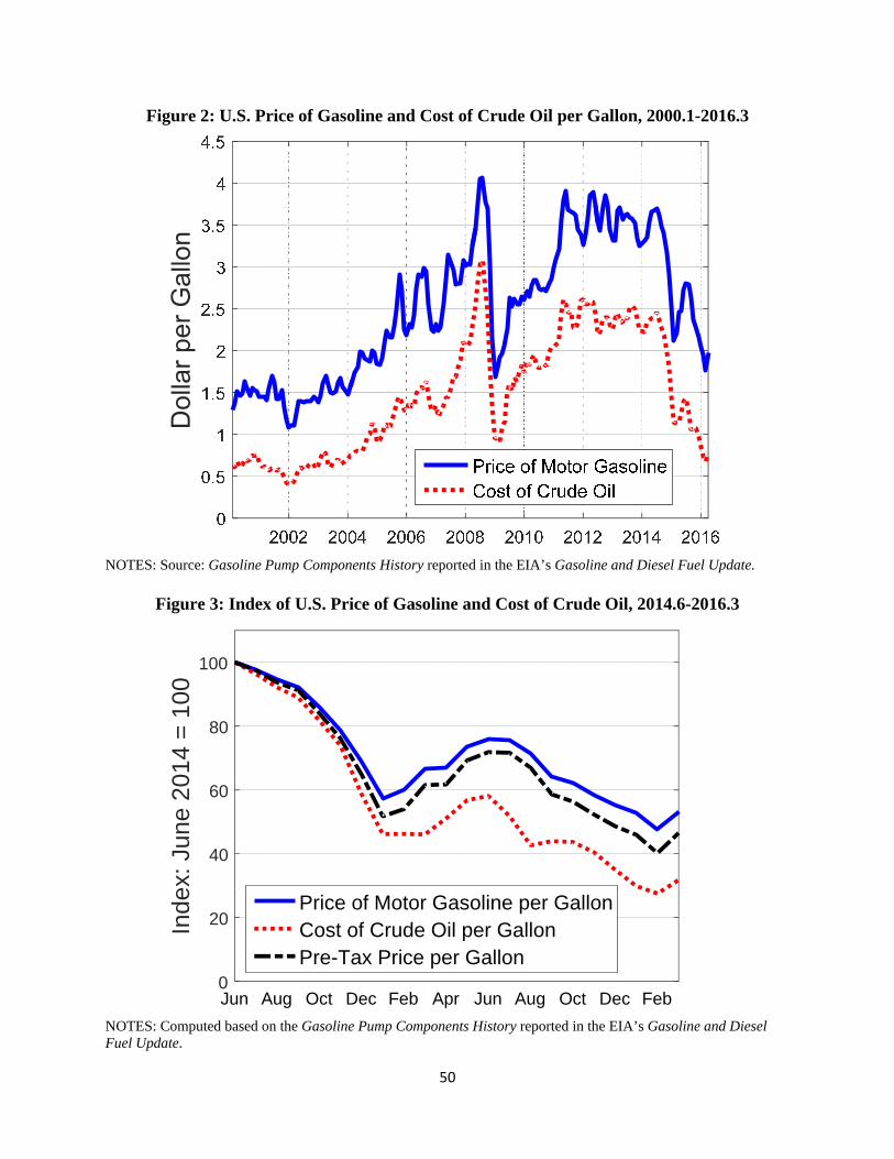
50
0
20
40
60
80
100
Inde
x: J
une
2014
= 1
00
Jun Aug Oct Dec Feb Apr Jun Aug Oct Dec Feb
Price of Motor Gasoline per GallonCost of Crude Oil per GallonPre-Tax Price per Gallon
Figure 2: U.S. Price of Gasoline and Cost of Crude Oil per Gallon, 2000.1-2016.3
NOTES: Source: Gasoline Pump Components History reported in the EIA’s Gasoline and Diesel Fuel Update.
Figure 3: Index of U.S. Price of Gasoline and Cost of Crude Oil, 2014.6-2016.3
NOTES: Computed based on the Gasoline Pump Components History reported in the EIA’s Gasoline and Diesel Fuel Update.

51
2010 2011 2012 2013 2014 2015 20162.5
2.6
2.7
2.8
2.9
3
3.1
3.2
3.3
3.4
3.5
Mill
ions
of M
iles
106
-6
-4
-2
0
2
4
6
8
10
Per
cent
Jul Sep Nov Jan Mar May Jul Sep Nov Jan Mar
Figure 4: Cumulative Change in U.S. Consumption of Motor Gasoline since 2014.6
NOTES: Based on the sum of transport, industrial and commercial gasoline consumption, as reported in the Monthly Energy Review, but seasonally adjusted by the authors.
Figure 5: Vehicle Miles Traveled
NOTES: Source: U.S. Federal Highway Administration. The vertical line marks June 2014.

52
1975 1980 1985 1990 1995 2000 2005 2010 2015
-20
0
20
Per
cent
Changes in U.S. Real Price of Gasoline and Other Motor Fuel
1975 1980 1985 1990 1995 2000 2005 2010 20150
5
Per
cent
Share of Gasoline in Total Consumer Expenditures
1975 1980 1985 1990 1995 2000 2005 2010 2015
-0.5
0
0.5
Per
cent
Shocks to U.S. Consumers' Purchasing Power
2007 2008 2009 2010 2011 2012 2013 2014 2015 20160
50
100
150
200
250
300
350
400
450
500
Cen
ts
Current Gas Price + MSC Expected Change in Gas PriceCurrent Gas Price + MSC Inflation Expectation
Figure 6: Michigan Consumer Survey 1-Year-Ahead Gasoline Price Expectations, 2006.2-2016.3
NOTES: The gasoline price expectation is obtained by adding the median expected change in gasoline prices over the next 12 months from the Michigan Survey of Consumers to the average U.S. price of gasoline from the Monthly Energy Review. The survey measure closely tracks the no-change forecast of the price of gasoline adjusted for the median expected change in the price level over the next 12 months, as reported in the Michigan Survey of Consumers, as previously noted by Anderson et al. (2013).
Figure 7: Measuring Shocks to Consumers’ Purchasing Power, 1970.2-2016.3
NOTES: All consumer expenditure and deflator data are from the BEA.
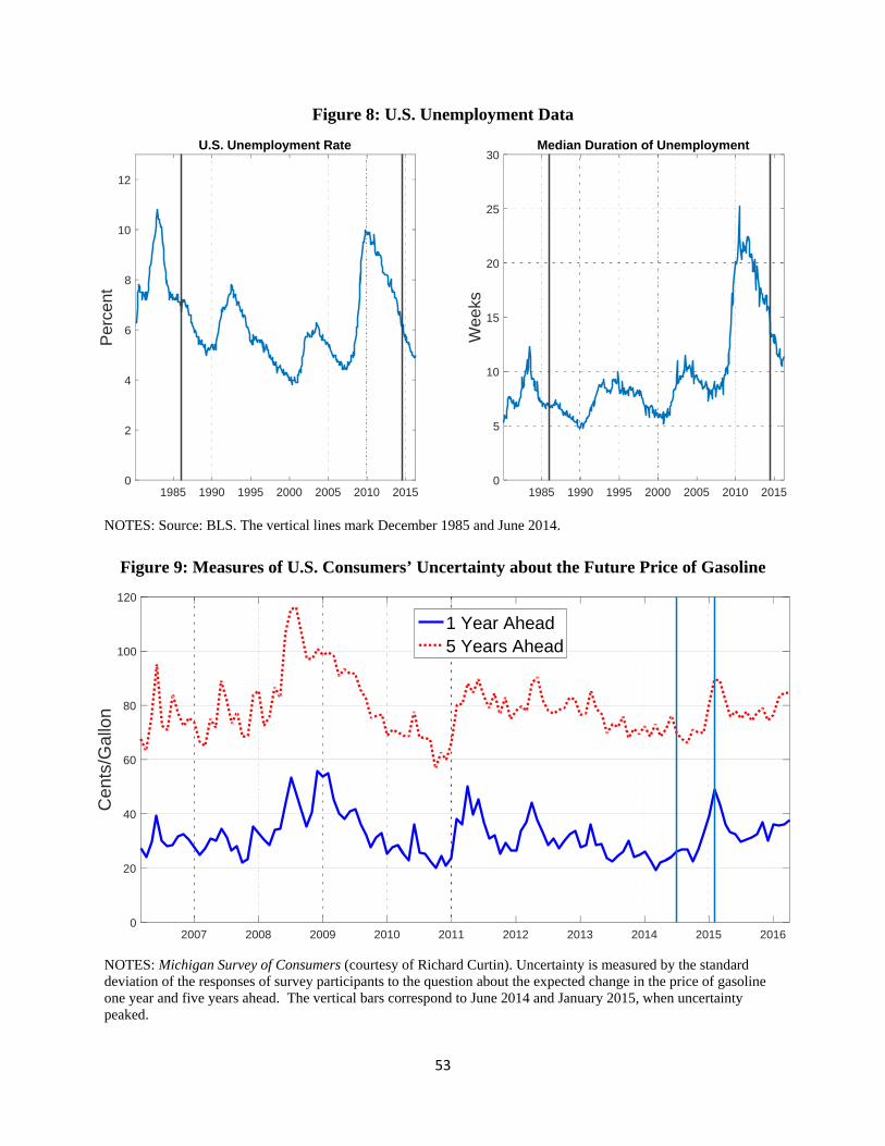
53
2007 2008 2009 2010 2011 2012 2013 2014 2015 20160
20
40
60
80
100
120
Cen
ts/G
allo
n
1 Year Ahead5 Years Ahead
1985 1990 1995 2000 2005 2010 20150
2
4
6
8
10
12
Per
cent
U.S. Unemployment Rate
1985 1990 1995 2000 2005 2010 20150
5
10
15
20
25
30
Wee
ks
Median Duration of Unemployment
Figure 8: U.S. Unemployment Data
NOTES: Source: BLS. The vertical lines mark December 1985 and June 2014.
Figure 9: Measures of U.S. Consumers’ Uncertainty about the Future Price of Gasoline
NOTES: Michigan Survey of Consumers (courtesy of Richard Curtin). Uncertainty is measured by the standard deviation of the responses of survey participants to the question about the expected change in the price of gasoline one year and five years ahead. The vertical bars correspond to June 2014 and January 2015, when uncertainty peaked.

54
2011 2012 2013 2014 2015 20160
2
4
6
8
10
12
Mill
ions
AutosLight trucks
2011 2012 2013 2014 2015 20160
0.01
0.02
0.03
0.04
0.05
0.06
0.07
0.08
Mill
ions
HEVPHEV+EREVBEVAll
2015 201616
16.5
17
17.5
18
18.5
Mill
ions
Sales of Autos and Light Trucks (BEA)
2015 2016
130
140
150
160
Inde
x
Current Buying Conditions for Vehicles (Michigan Survey of Consumers)
Figure 10: Did Uncertainty about Gas Prices Prevent Consumers from Buying Vehicles? NOTES: The vertical bars correspond to June 2014 and January 2015.
Figure 11: Decomposition of Vehicle Sales NOTES: Left panel: Aggregate of domestic and foreign sales. Source: BEA. Right panel: HEV = hybrid vehicles; BEV = battery powered vehicles; PHEV = plug-in hybrid vehicles; EREV = extended-range electric vehicles. Source: Electric Drive Transportation Association. The vertical line marks June 2014.

55
2010 2011 2012 2013 2014 2015 20160
20
40
60
80
Inde
x
Figure 12: U.S. Banking Stock Market Index
NOTES: The plot shows monthly averages of the KBW bank index for January 2009 through May 2016. The index includes 24 U.S. banking stocks and is traded on the Philadelphia stock exchange. The vertical line marks June 2014.


