Technical Report no. 2005:22
LYDIAN: User’s Guide
Phuong Hoai Ha, Boris Koldehofe, Marina Papatriantafilou,Philippas Tsigas
Department of Computing Science and EngineeringChalmers University of Technology and Göteborg University
SE-412 96 Göteborg, Sweden
Göteborg, 2005

Department of Computing Science and EngineeringDivision of Computing ScienceChalmers University of Technology and Göteborg UniversitySE-412 96 Göteborg, Sweden
Technical Report no. 2005:22ISSN: 1652-926X
Göteborg, Sweden, December 2005.
Contents
. . . . . . . . . . . . . . . . . . . . . . . . . . . . . . . . . . . . . . . . . . . . . . . . . . . . . . . . . . . . . 3
1 Introduction 4
2 Installation 42.1 In general . . .. . . . . . . . . . . . . . . . . . . . . . . . . . . . . . . . . . . . . . . . . . . . . . . . . . 42.2 An example: In the Chalmers computer system . .. . . . . . . . . . . . . . . . . . . . . . . . . . . . . . . 4
3 Getting started: The LYDIAN graphical user interface 53.1 Menu system .. . . . . . . . . . . . . . . . . . . . . . . . . . . . . . . . . . . . . . . . . . . . . . . . . . 53.2 A simple example. . . . . . . . . . . . . . . . . . . . . . . . . . . . . . . . . . . . . . . . . . . . . . . . . 6
3.2.1 Broadcast with acknowledgement algorithm. . . . . . . . . . . . . . . . . . . . . . . . . . . . . . . 63.2.2 Running an experiment . .. . . . . . . . . . . . . . . . . . . . . . . . . . . . . . . . . . . . . . . . 73.2.3 Experiment dialogue window . .. . . . . . . . . . . . . . . . . . . . . . . . . . . . . . . . . . . . 7
3.3 Graphical animation windows . .. . . . . . . . . . . . . . . . . . . . . . . . . . . . . . . . . . . . . . . . 93.3.1 Basic view . . .. . . . . . . . . . . . . . . . . . . . . . . . . . . . . . . . . . . . . . . . . . . . . 93.3.2 Causality view .. . . . . . . . . . . . . . . . . . . . . . . . . . . . . . . . . . . . . . . . . . . . . 103.3.3 Information on events of processors. . . . . . . . . . . . . . . . . . . . . . . . . . . . . . . . . . . 103.3.4 Overall view on sent messages . .. . . . . . . . . . . . . . . . . . . . . . . . . . . . . . . . . . . . 113.3.5 Application’s processor utilization. . . . . . . . . . . . . . . . . . . . . . . . . . . . . . . . . . . . 11
3.4 ASCII monitoring. . . . . . . . . . . . . . . . . . . . . . . . . . . . . . . . . . . . . . . . . . . . . . . . . 123.4.1 Main window . .. . . . . . . . . . . . . . . . . . . . . . . . . . . . . . . . . . . . . . . . . . . . . 123.4.2 Process window. . . . . . . . . . . . . . . . . . . . . . . . . . . . . . . . . . . . . . . . . . . . . 143.4.3 Interactive commands to interface. . . . . . . . . . . . . . . . . . . . . . . . . . . . . . . . . . . . 14
4 LYDIAN model 154.1 Simulator model. . . . . . . . . . . . . . . . . . . . . . . . . . . . . . . . . . . . . . . . . . . . . . . . . . 154.2 Protocol model . . . . . . . . . . . . . . . . . . . . . . . . . . . . . . . . . . . . . . . . . . . . . . . . . . 154.3 Network model . . . . . . . . . . . . . . . . . . . . . . . . . . . . . . . . . . . . . . . . . . . . . . . . . . 16
4.3.1 Flexible timing conditions. . . . . . . . . . . . . . . . . . . . . . . . . . . . . . . . . . . . . . . . 164.3.2 Link failure support. . . . . . . . . . . . . . . . . . . . . . . . . . . . . . . . . . . . . . . . . . . . 18
4.4 Assumptions made for the simulated systems . . .. . . . . . . . . . . . . . . . . . . . . . . . . . . . . . . 18
5 Making new protocols 195.1 Design. . . . . . . . . . . . . . . . . . . . . . . . . . . . . . . . . . . . . . . . . . . . . . . . . . . . . . . 195.2 System structure. . . . . . . . . . . . . . . . . . . . . . . . . . . . . . . . . . . . . . . . . . . . . . . . . . 20
5.2.1 Message structure. . . . . . . . . . . . . . . . . . . . . . . . . . . . . . . . . . . . . . . . . . . . . 205.2.2 Node Process Control Block (PCB) and local variables. . . . . . . . . . . . . . . . . . . . . . . . . 21
5.3 Implementation. . . . . . . . . . . . . . . . . . . . . . . . . . . . . . . . . . . . . . . . . . . . . . . . . . 235.4 Adding new protocols to LYDIAN. . . . . . . . . . . . . . . . . . . . . . . . . . . . . . . . . . . . . . . . 24
6 Making new networks 266.1 Network description files. . . . . . . . . . . . . . . . . . . . . . . . . . . . . . . . . . . . . . . . . . . . . 27
7 DIAS reference 287.1 Debugging and metrics .. . . . . . . . . . . . . . . . . . . . . . . . . . . . . . . . . . . . . . . . . . . . . 28
7.1.1 Header . . . . . . . . . . . . . . . . . . . . . . . . . . . . . . . . . . . . . . . . . . . . . . . . . . 287.1.2 Tracing part . . .. . . . . . . . . . . . . . . . . . . . . . . . . . . . . . . . . . . . . . . . . . . . . 287.1.3 Footer .. . . . . . . . . . . . . . . . . . . . . . . . . . . . . . . . . . . . . . . . . . . . . . . . . . 29
7.2 Available routines in the simulator. . . . . . . . . . . . . . . . . . . . . . . . . . . . . . . . . . . . . . . . 297.2.1 Message delivering . . .. . . . . . . . . . . . . . . . . . . . . . . . . . . . . . . . . . . . . . . . 297.2.2 Message and queue manipulation. . . . . . . . . . . . . . . . . . . . . . . . . . . . . . . . . . . . 30
7.2.3 Timer manipulation. . . . . . . . . . . . . . . . . . . . . . . . . . . . . . . . . . . . . . . . . . . . 307.2.4 Debug and user interface .. . . . . . . . . . . . . . . . . . . . . . . . . . . . . . . . . . . . . . . . 317.2.5 List handling . .. . . . . . . . . . . . . . . . . . . . . . . . . . . . . . . . . . . . . . . . . . . . . 327.2.6 Protocol stopping and restarting .. . . . . . . . . . . . . . . . . . . . . . . . . . . . . . . . . . . . 327.2.7 Randomizing . .. . . . . . . . . . . . . . . . . . . . . . . . . . . . . . . . . . . . . . . . . . . . . 33
8 POLKA Animation Designer’s Package 348.1 Animator level . . . . . . . . . . . . . . . . . . . . . . . . . . . . . . . . . . . . . . . . . . . . . . . . . . 34
8.1.1 Entry points . . .. . . . . . . . . . . . . . . . . . . . . . . . . . . . . . . . . . . . . . . . . . . . . 348.1.2 Example . . . . . . . . . . . . . . . . . . . . . . . . . . . . . . . . . . . . . . . . . . . . . . . . . 35
8.2 Animation Views . . . . . . . . . . . . . . . . . . . . . . . . . . . . . . . . . . . . . . . . . . . . . . . . . 368.2.1 Entry Points . . .. . . . . . . . . . . . . . . . . . . . . . . . . . . . . . . . . . . . . . . . . . . . . 368.2.2 Example Definition. . . . . . . . . . . . . . . . . . . . . . . . . . . . . . . . . . . . . . . . . . . . 38
8.3 Objects in an Animation View . .. . . . . . . . . . . . . . . . . . . . . . . . . . . . . . . . . . . . . . . . 388.3.1 Loc . . . . . . . . . . . . . . . . . . . . . . . . . . . . . . . . . . . . . . . . . . . . . . . . . . . . 388.3.2 AnimObjects . .. . . . . . . . . . . . . . . . . . . . . . . . . . . . . . . . . . . . . . . . . . . . . 398.3.3 Action . . . . . . . . . . . . . . . . . . . . . . . . . . . . . . . . . . . . . . . . . . . . . . . . . . . 43
A The source code of algorithm Broadcast with ACK 50
B The source code of Ricart and Agrawala’s Resource Allocation algorithm 51
List of Figures
. . . . . . . . . . . . . . . . . . . . . . . . . . . . . . . . . . . . . . . . . . . . . . . . . . . . . . . . . . . . . 31 Lydian user interface . .. . . . . . . . . . . . . . . . . . . . . . . . . . . . . . . . . . . . . . . . . . . . . 42 Lydian architecture . . .. . . . . . . . . . . . . . . . . . . . . . . . . . . . . . . . . . . . . . . . . . . . . 53 Main Lydian window . . . . . . . . . . . . . . . . . . . . . . . . . . . . . . . . . . . . . . . . . . . . . . . 74 Polka control panel . . .. . . . . . . . . . . . . . . . . . . . . . . . . . . . . . . . . . . . . . . . . . . . . 75 Animation control window . . . . . . . . . . . . . . . . . . . . . . . . . . . . . . . . . . . . . . . . . . . . 76 Experiment dialogue window . . .. . . . . . . . . . . . . . . . . . . . . . . . . . . . . . . . . . . . . . . . 87 Basic view of experiment Broadcast with ACK . .. . . . . . . . . . . . . . . . . . . . . . . . . . . . . . . 108 Causality view of experiment Broadcast with ACK. . . . . . . . . . . . . . . . . . . . . . . . . . . . . . . 119 Information on processor’s events. . . . . . . . . . . . . . . . . . . . . . . . . . . . . . . . . . . . . . . . 1110 Overall view on sent messages of experiment Broadcast with ACK . .. . . . . . . . . . . . . . . . . . . . . 1211 Processor utilization of experiment Broadcast with ACK . .. . . . . . . . . . . . . . . . . . . . . . . . . . 1312 Ascii monitoring of experiment Broadcast with ACK. . . . . . . . . . . . . . . . . . . . . . . . . . . . . . 1313 The framework of protocol source code .. . . . . . . . . . . . . . . . . . . . . . . . . . . . . . . . . . . . 2314 Initialization part of protocol Broadcast with ACK .. . . . . . . . . . . . . . . . . . . . . . . . . . . . . . . 2315 Procedures of protocol Broadcast with ACK. . . . . . . . . . . . . . . . . . . . . . . . . . . . . . . . . . . 2416 New protocol generation interface. . . . . . . . . . . . . . . . . . . . . . . . . . . . . . . . . . . . . . . . 2517 New network generation interface. . . . . . . . . . . . . . . . . . . . . . . . . . . . . . . . . . . . . . . . 27
List of Tables
. . . . . . . . . . . . . . . . . . . . . . . . . . . . . . . . . . . . . . . . . . . . . . . . . . . . . . . . . . . . . 31 The design of algorithm Broadcast with ACK . . .. . . . . . . . . . . . . . . . . . . . . . . . . . . . . . . 19
1 Introduction
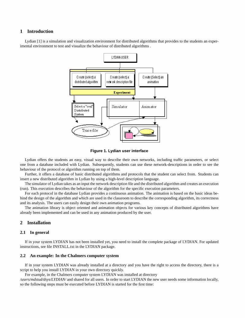
Lydian [1] is a simulation and visualization environment for distributed algorithms that provides to the students an exper-imental environment to test and visualize the behaviour of distributed algorithms .
Figure 1. Lydian user interface
Lydian offers the students an easy, visual way to describe their own networks, including traffic parameters, or selectone from a database included with Lydian. Subsequently, students can use these network-descriptions in order to see thebehaviour of the protocol or algorithm running on top of them.
Further, it offers a database of basic distributed algorithms and protocols that the student can select from. Students caninsert a new distributed algorithm in Lydian by using a high-level description language.
The simulator of Lydian takes as an input the network description file and the distributed algorithm and creates an execution(run). This execution describes the behaviour of the algorithm for the specific execution parameters.
For each protocol in the database Lydian provides a continuous animation. The animation is based on the basic ideas be-hind the design of the algorithm and which are used in the classroom to describe the corresponding algorithm, its correctnessand its analysis. The users can easily design their own animation programs.
The animation library is object oriented and animation objects for various key concepts of distributed algorithms havealready been implemented and can be used in any animation produced by the user.
2 Installation
2.1 In general
If in your system LYDIAN has not been installed yet, you need to install the complete package of LYDIAN. For updatedinstructions, see file INSTALL.txt in the LYDIAN package.
2.2 An example: In the Chalmers computer system
If in your system LYDIAN was already installed at a directory and you have the right to access the directory, there is ascript to help you install LYDIAN in your own directory quickly.
For example, in the Chalmers computer system LYDIAN was installed at directory/users/mdstud/dsys/LYDIAN/ and shared for all users. In order to start LYDIAN the new user needs some information locally,so the following steps must be executed before LYDIAN is started for the first time:
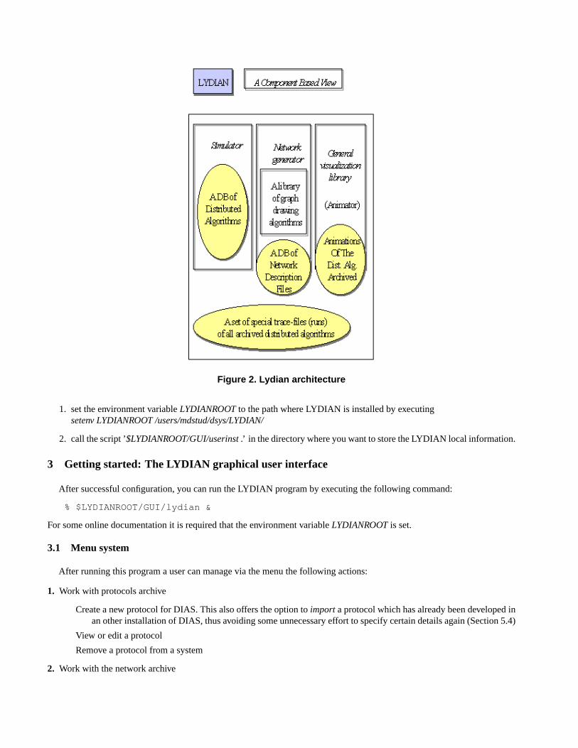
Figure 2. Lydian architecture
1. set the environment variableLYDIANROOT to the path where LYDIAN is installed by executingsetenv LYDIANROOT /users/mdstud/dsys/LYDIAN/
2. call the script ’$LYDIANROOT/GUI/userinst .’ in the directory where you want to store the LYDIAN local information.
3 Getting started: The LYDIAN graphical user interface
After successful configuration, you can run the LYDIAN program by executing the following command:
% $LYDIANROOT/GUI/lydian &
For some online documentation it is required that the environment variableLYDIANROOT is set.
3.1 Menu system
After running this program a user can manage via the menu the following actions:
1. Work with protocols archive
Create a new protocol for DIAS. This also offers the option toimport a protocol which has already been developed inan other installation of DIAS, thus avoiding some unnecessary effort to specify certain details again (Section 5.4)
View or edit a protocol
Remove a protocol from a system
2. Work with the network archive
Create a new network description file
View or edit a network description file
Delete a network description file
3. Work with the experiment archive
Create a new network experiment description file
View or edit an existing experiment description file
Delete an experiment description file
4. Load and execute an experiment. (cf. also subsection 3.2.3, later in this document). The simulator of DIAS is invoked tosimulate the required protocol with all parameters specified in the respective experiment.
This option includes also the animation of the experiment. The animation can run on-line with the simulator (theanimator program consumes via apipe command the output produced by the simulation execution) or it can run off-line, by having the animator program take as input one of the debug (trace) files that have been produced by thesimulation of the respective protocol. In either case, the animation is triggered by the experiment dialogue box.
5. Run the on-line help system of DIAS
Each action has the corresponding item in the menu. As an example, we describe actions for one of these objects, namelyfor the protocol archive menu.
At the current version, upon choosing the creation of a new protocol, the system offers the option to create a protocolright from the beginning, or to import one that has already been created in DIAS. In either case, the system opens an xterm,through which it interacts with the (old) DIAS sequential procedure for the creation orimporting of a protocol (Section 5.4).When we use the item for editing of protocols, first the select dialog appears. There, we can choose via mouse one protocoland by pressing the select button we can invocatevi editor for its editing. In this dialog, the cancel button can be used toreturn to the main menu without performing any action. Removal from the archive is the last action supported for protocols.The dialog for this action can be easily invoked via the menu.
The same functionality is supported for manipulating the network archive and the experiment archive. There is only oneexception for the experiment archive and it will be discussed later. For convenience it is good to use the on-line-help systemthat desribes all procedures in DIAS.
3.2 A simple example
As a way of introducing LYDIAN, we will go through the sample experiment, which uses the broadcast with ACKalgorithm, one of available experiments in LYDIAN.
3.2.1 Broadcast with acknowledgement algorithm
This algorithm is the following. At the beginning an initiator process sends the broadcast message to all its neighbours. Theprocess which receives the broadcast message for the first time sends the message to all its adjacent processes except forthe one from which it received the message. In addition to this, it marks the sender of the first received broadcast messageas its parent. Every process keeps track of broadcast messages it sends to adjacent processes by storing the receiver ofeach message in a set of expected acknowledgements, calledack. As long asack is not empty the process waits to receiveacknowledgements from processes stored in this set. On receiving an acknowledgement it deletes the sender fromack. Whenack is an empty set then all acknowledgements are received, and the process sends an acknowledgement to its parent node andterminates the algorithm. Processes which receive a message broadcast despite having already decided for their parent nodereply with an acknowledgement. This guarantees that every broadcast message will be answered by an acknowledgement.The algorithm is finished when the initiator received all acknowledgements.
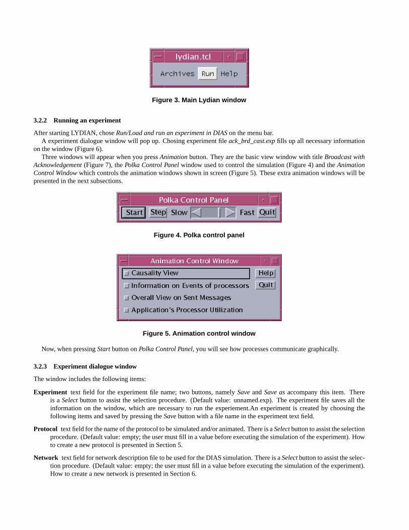
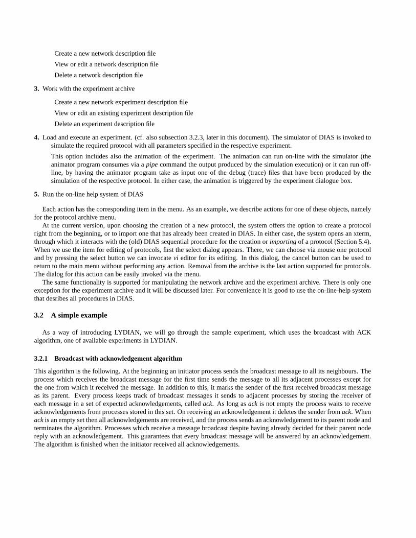
Figure 3. Main Lydian window
3.2.2 Running an experiment
After starting LYDIAN, choseRun/Load and run an experiment in DIAS on the menu bar.A experiment dialogue window will pop up. Chosing experiment fileack_brd_cast.exp fills up all necessary information
on the window (Figure 6).Three windows will appear when you pressAnimation button. They are the basic view window with titleBroadcast with
Acknowledgement (Figure 7), thePolka Control Panel window used to control the simulation (Figure 4) and theAnimationControl Window which controls the animation windows shown in screen (Figure 5). These extra animation windows will bepresented in the next subsections.
Figure 4. Polka control panel
Figure 5. Animation control window
Now, when pressingStart button onPolka Control Panel, you will see how processes communicate graphically.
3.2.3 Experiment dialogue window
The window includes the following items:
Experiment text field for the experiment file name; two buttons, namelySave andSave as accompany this item. Thereis a Select button to assist the selection procedure. (Default value: unnamed.exp). The experiment file saves all theinformation on the window, which are necessary to run the experiement.An experiment is created by choosing thefollowing items and saved by pressing theSave button with a file name in the experiment text field.
Protocol text field for the name of the protocol to be simulated and/or animated. There is aSelect button to assist the selectionprocedure. (Default value: empty; the user must fill in a value before executing the simulation of the experiment). Howto create a new protocol is presented in Section 5.
Network text field for network description file to be used for the DIAS simulation. There is aSelect button to assist the selec-tion procedure. (Default value: empty; the user must fill in a value before executing the simulation of the experiment).How to create a new network is presented in Section 6.
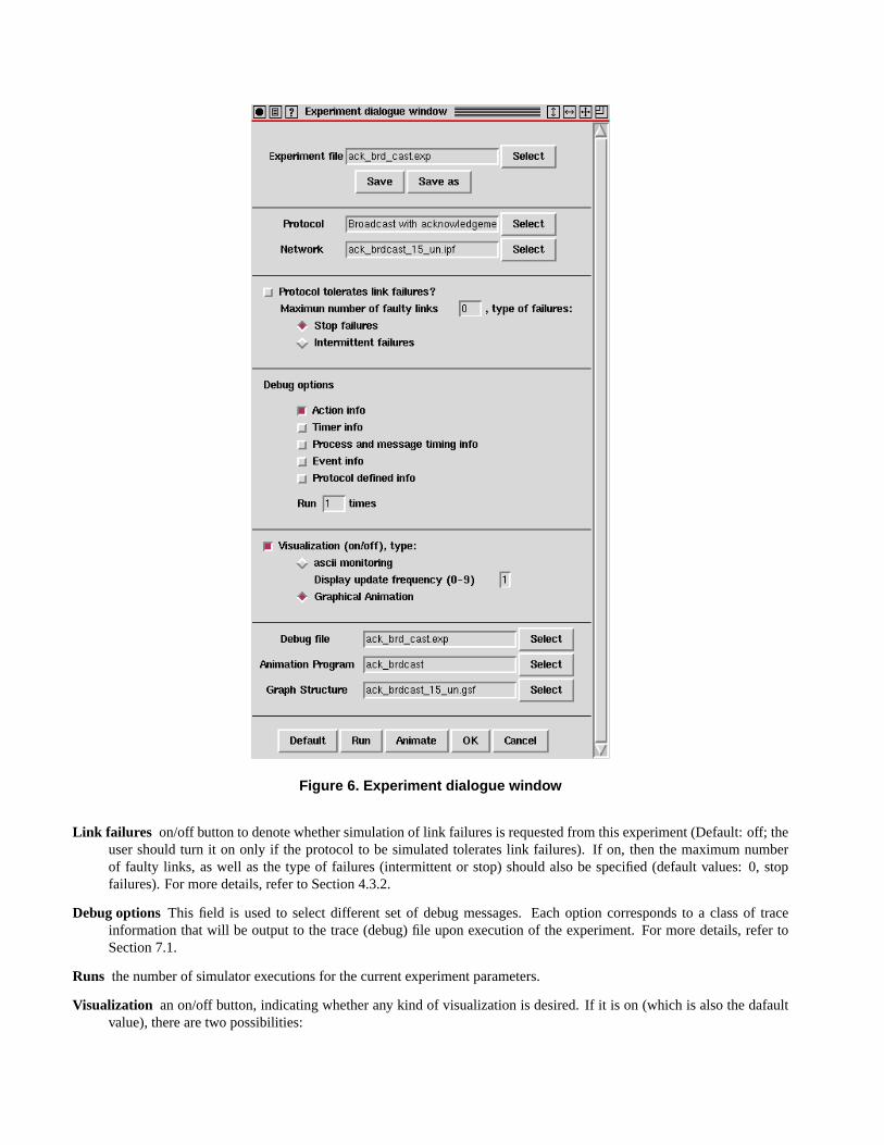
Figure 6. Experiment dialogue window
Link failures on/off button to denote whether simulation of link failures is requested from this experiment (Default: off; theuser should turn it on only if the protocol to be simulated tolerates link failures). If on, then the maximum numberof faulty links, as well as the type of failures (intermittent or stop) should also be specified (default values: 0, stopfailures). For more details, refer to Section 4.3.2.
Debug options This field is used to select different set of debug messages. Each option corresponds to a class of traceinformation that will be output to the trace (debug) file upon execution of the experiment. For more details, refer toSection 7.1.
Runs the number of simulator executions for the current experiment parameters.
Visualization an on/off button, indicating whether any kind of visualization is desired. If it is on (which is also the dafaultvalue), there are two possibilities:
ascii monitoring : this is a visual (ascii) output interafce, which monitors the execution and which is provided directlyfrom the DIAS simulation (for non-multiple executions). For more details, refer to Section 3.4
Graphical Animation : This corresponds to execution of the corresponding animation program for the protocol thatis chosen for simulation. In this case theAnimation Program has to be specified, see bellow.Note: at the present version the mapping is not automatic; the user should be aware of this choice.
Debug file text field for the debug file name (if empty, the system will chose automatically a name, equal todebug.experiment_file_name).There is aselect button to assist the selection procedure.
Animation Program text field for the name of an animation program (which, as explained earlier, should be suitable toanimate executions of the chosen protocol). There is aselect button to assist the selection procedure. (Default value:the animator program specified in the configuaration file)
Buttons Finally, there is a set of buttons to support standard functions, such asCancel andOK, as well as the followingprocedures:
Default for setting default values for dialog fields. It means, in the most cases to clear them. It is useful to create acompletely new experiment description.
Run to invoke the DIAS simulator with the values specified in the current experiment dialogue window. Before startingthe execution the current directory is set to directoryprotocols_path (see Section 2.1). If theVisualization buttonis on and theGraphical Animation possibility has been chosen the animation program will also be executedbesides the simulation. This corresponds to the on-line execution of the animation.
Animate to invoke the animation program shown in the respective field in the dialogue window. This corresponds to theoff-line execution of the animation, i.e. the simulator will not be invoked. Before starting this program the currentdirectory is set to directoryanimators_path (see Section 2.1).Note: the Visalization button should be on and the Graphical Animation possibility should have been chosen; other-wise, nothing will happen in response to pressing this button.
Note: all programs specified in the dialogue window must be in the corresponding path given in the configuration file, asdescribed in the previous section; otherwise, the file name should be pended with the path where it can be found.
3.3 Graphical animation windows
3.3.1 Basic view
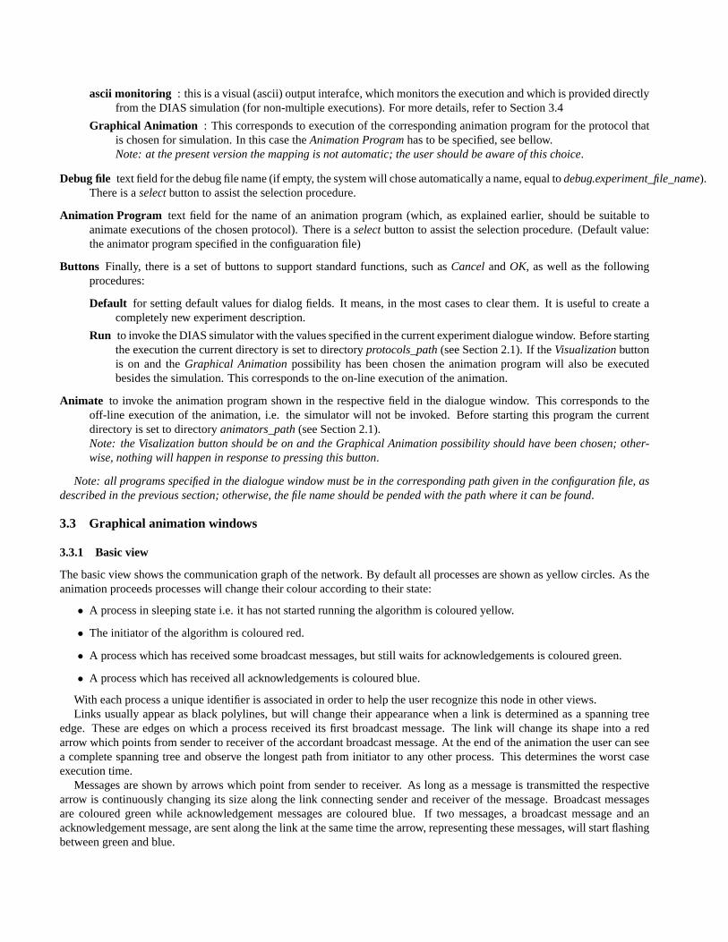
The basic view shows the communication graph of the network. By default all processes are shown as yellow circles. As theanimation proceeds processes will change their colour according to their state:
• A process in sleeping state i.e. it has not started running the algorithm is coloured yellow.
• The initiator of the algorithm is coloured red.
• A process which has received some broadcast messages, but still waits for acknowledgements is coloured green.
• A process which has received all acknowledgements is coloured blue.
With each process a unique identifier is associated in order to help the user recognize this node in other views.Links usually appear as black polylines, but will change their appearance when a link is determined as a spanning tree
edge. These are edges on which a process received its first broadcast message. The link will change its shape into a redarrow which points from sender to receiver of the accordant broadcast message. At the end of the animation the user can seea complete spanning tree and observe the longest path from initiator to any other process. This determines the worst caseexecution time.
Messages are shown by arrows which point from sender to receiver. As long as a message is transmitted the respectivearrow is continuously changing its size along the link connecting sender and receiver of the message. Broadcast messagesare coloured green while acknowledgement messages are coloured blue. If two messages, a broadcast message and anacknowledgement message, are sent along the link at the same time the arrow, representing these messages, will start flashingbetween green and blue.
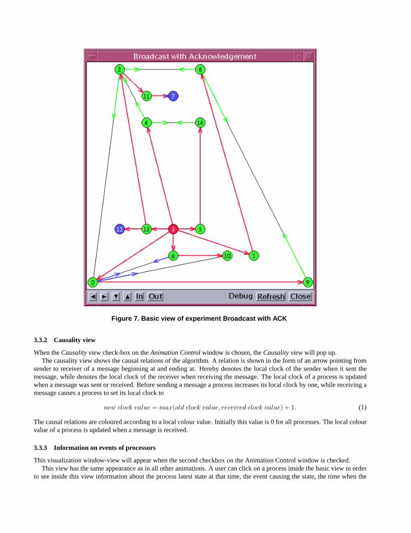
Figure 7. Basic view of experiment Broadcast with ACK
3.3.2 Causality view
When theCausality view check-box on theAnimation Control window is chosen, theCausality view will pop up.The causality view shows the causal relations of the algorithm. A relation is shown in the form of an arrow pointing from
sender to receiver of a message beginning at and ending at. Hereby denotes the local clock of the sender when it sent themessage, while denotes the local clock of the receiver when receiving the message. The local clock of a process is updatedwhen a message was sent or received. Before sending a message a process increases its local clock by one, while receiving amessage causes a process to set its local clock to
new clock value = max(old clock value, received clock value) + 1. (1)
The causal relations are coloured according to a local colour value. Initially this value is 0 for all processes. The local colourvalue of a process is updated when a message is received.
3.3.3 Information on events of processors
This visualization window-view will appear when the second checkbox on the Animation Control window is checked.This view has the same appearance as in all other animations. A user can click on a process inside the basic view in order
to see inside this view information about the process latest state at that time, the event causing the state, the time when the
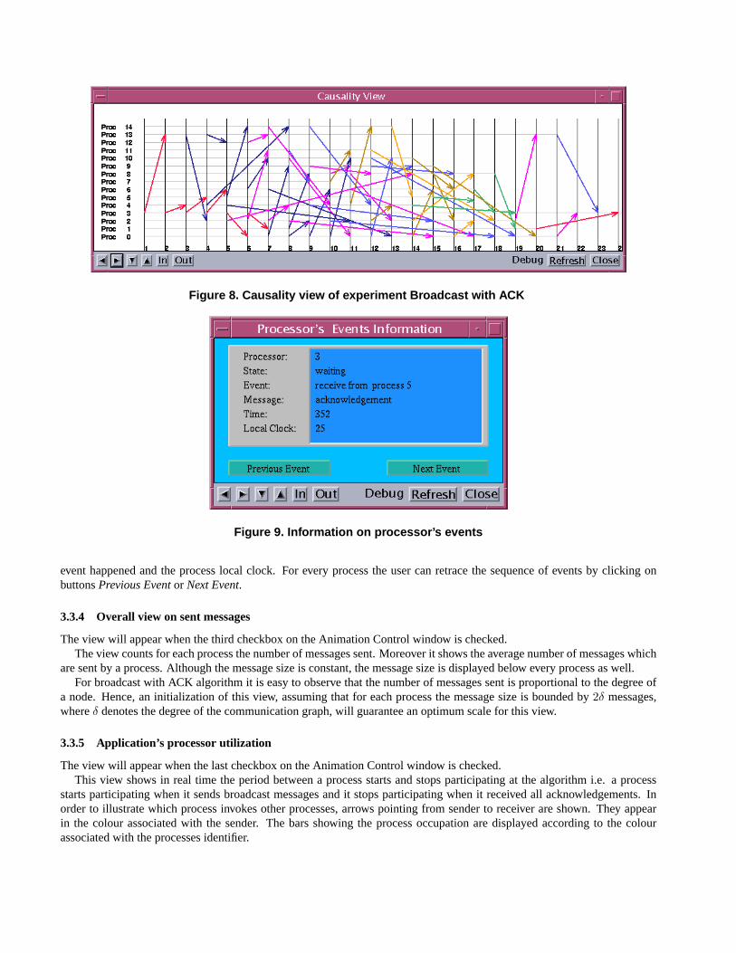
Figure 8. Causality view of experiment Broadcast with ACK
Figure 9. Information on processor’s events
event happened and the process local clock. For every process the user can retrace the sequence of events by clicking onbuttonsPrevious Event or Next Event.
3.3.4 Overall view on sent messages
The view will appear when the third checkbox on the Animation Control window is checked.The view counts for each process the number of messages sent. Moreover it shows the average number of messages which
are sent by a process. Although the message size is constant, the message size is displayed below every process as well.For broadcast with ACK algorithm it is easy to observe that the number of messages sent is proportional to the degree of
a node. Hence, an initialization of this view, assuming that for each process the message size is bounded by2δ messages,whereδ denotes the degree of the communication graph, will guarantee an optimum scale for this view.
3.3.5 Application’s processor utilization
The view will appear when the last checkbox on the Animation Control window is checked.This view shows in real time the period between a process starts and stops participating at the algorithm i.e. a process
starts participating when it sends broadcast messages and it stops participating when it received all acknowledgements. Inorder to illustrate which process invokes other processes, arrows pointing from sender to receiver are shown. They appearin the colour associated with the sender. The bars showing the process occupation are displayed according to the colourassociated with the processes identifier.
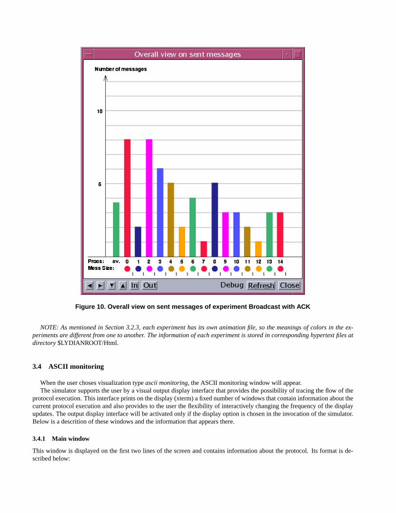
Figure 10. Overall view on sent messages of experiment Broadcast with ACK
NOTE: As mentioned in Section 3.2.3, each experiment has its own animation file, so the meanings of colors in the ex-periments are different from one to another. The information of each experiment is stored in corresponding hypertext files atdirectory $LYDIANROOT/Html.
3.4 ASCII monitoring
When the user choses visualization typeascii monitoring, the ASCII monitoring window will appear.The simulator supports the user by a visual output display interface that provides the possibility of tracing the flow of the
protocol execution. This interface prints on the display (xterm) a fixed number of windows that contain information about thecurrent protocol execution and also provides to the user the flexibility of interactively changing the frequency of the displayupdates. The output display interface will be activated only if the display option is chosen in the invocation of the simulator.Below is a descrition of these windows and the information that appears there.
3.4.1 Main window
This window is displayed on the first two lines of the screen and contains information about the protocol. Its format is de-scribed below:
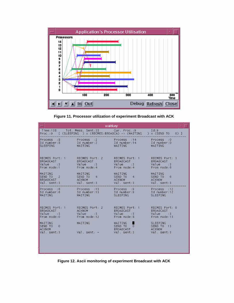
Figure 11. Processor utilization of experiment Broadcast with ACK
Figure 12. Ascii monitoring of experiment Broadcast with ACK
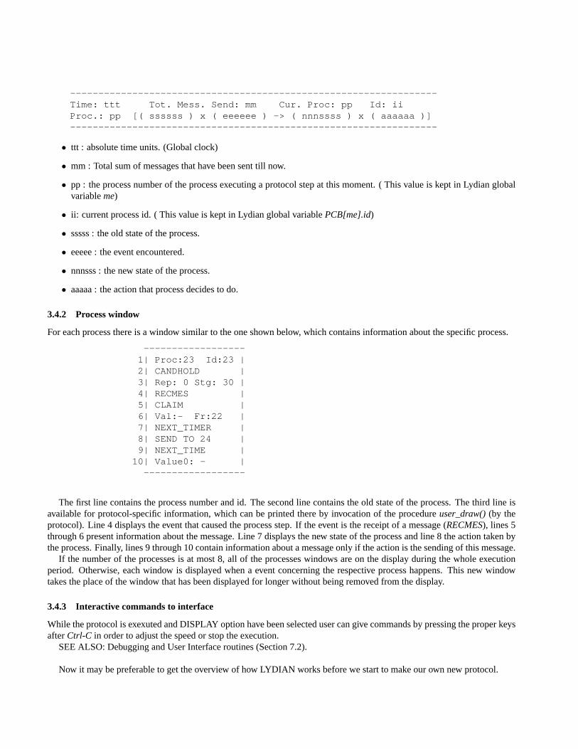
-----------------------------------------------------------------Time: ttt Tot. Mess. Send: mm Cur. Proc: pp Id: iiProc.: pp [( ssssss ) x ( eeeeee ) -> ( nnnssss ) x ( aaaaaa )]-----------------------------------------------------------------
• ttt : absolute time units. (Global clock)
• mm : Total sum of messages that have been sent till now.
• pp : the process number of the process executing a protocol step at this moment. ( This value is kept in Lydian globalvariableme)
• ii: current process id. ( This value is kept in Lydian global variablePCB[me].id)
• sssss : the old state of the process.
• eeeee : the event encountered.
• nnnsss : the new state of the process.
• aaaaa : the action that process decides to do.
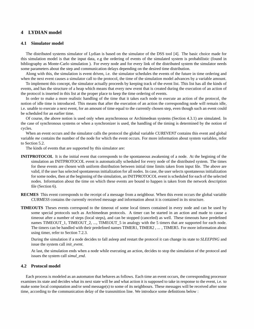
3.4.2 Process window
For each process there is a window similar to the one shown below, which contains information about the specific process.
------------------1| Proc:23 Id:23 |2| CANDHOLD |3| Rep: 0 Stg: 30 |4| RECMES |5| CLAIM |6| Val:- Fr:22 |7| NEXT_TIMER |8| SEND TO 24 |9| NEXT_TIME |10| Value0: - |------------------
The first line contains the process number and id. The second line contains the old state of the process. The third line isavailable for protocol-specific information, which can be printed there by invocation of the procedureuser_draw() (by theprotocol). Line 4 displays the event that caused the process step. If the event is the receipt of a message (RECMES), lines 5through 6 present information about the message. Line 7 displays the new state of the process and line 8 the action taken bythe process. Finally, lines 9 through 10 contain information about a message only if the action is the sending of this message.
If the number of the processes is at most 8, all of the processes windows are on the display during the whole executionperiod. Otherwise, each window is displayed when a event concerning the respective process happens. This new windowtakes the place of the window that has been displayed for longer without being removed from the display.
3.4.3 Interactive commands to interface
While the protocol isexexuted and DISPLAY option have been selected user can give commands by pressing the proper keysafterCtrl-C in order to adjust the speed or stop the execution.
SEE ALSO: Debugging and User Interface routines (Section 7.2).
Now it may be preferable to get the overview of how LYDIAN works before we start to make our own new protocol.
4 LYDIAN model
4.1 Simulator model
The distributed systems simulator of Lydian is based on the simulator of the DSS tool [4]. The basic choice made forthis simulation model is that the input data, e.g the ordering of events of the simulated system is probabilistic (found inbibliography as Monte-Carlo simulation ). For every node and for every link of the distributed system the simulator needssome parameters about the step and communication delays depending on the desired time distribution.
Along with this, the simulation is event driven, i.e. the simulator schedules the events of the future in time ordering andwhen the next event causes a simulator call to the protocol, the time of the simulation model advances by a variable amount.
To implement this concept, the simulator actually proceeds by keeping track of the event list. This list has all the kinds ofevents, and has the structure of a heap which means that every new event that is created during the execution of an action ofthe protocol is inserted in this list at the proper place to keep the time ordering of events.
In order to make a more realistic handling of the time that it takes each node to execute an action of the protocol, thenotion of idle time is introduced. This means that after the execution of an action the corresponding node will remain idle,i.e. unable to execute a next event, for an amount of time equal to the currently chosen step, even though such an event couldbe scheduled for an earlier time.
Of course, the above notion is used only when asynchronous or Archimedean systems (Section 4.3.1) are simulated. Inthe case of synchronous systems or when a synchronizer is used, the handling of the timing is determined by the notion ofcycles.
When an event occurs and the simulator calls the protocol the global variableCUREVENT contains this event and globalvariableme contains the number of the node for which the event occurs. For more information about system variables, referto Section 5.2.
The kinds of events that are supported by this simulator are:
INITPROTOCOL It is the initial event that corresponds to the spontaneous awakening of a node. At the begining of thesimulation an INITPROTOCOL event is automatically scheduled for every node of the distributed system. The timesfor these events are chosen with uniform distribution between initial time limits taken from input file. The above arevalid, if the user has selected spontaneous initialization for all nodes. In case, the user selects spontaneous initializationfor some nodes, then at the beginning of the simulation, an INITPROTOCOL event is scheduled for each of the selectednodes. Information about the time on which these events are bound to happen is taken from the network descriptionfile (Section 6).
RECMES This event corresponds to the receipt of a message from a neighbour. When this event occurs the global variableCURMESS contains the currently received message and information about it is contained in its structure.
TIMEOUTS Theses events correspond to the timeout of some local timers contained in every node and can be used bysome special protocols such as Archimedean protocols. A timer can be started in an action and made to cause atimeout after a number of steps (local steps), and can be stopped (canceled) as well. These timeouts have predefinednames TIMEOUT_1, TIMEOUT_2, ..., TIMEOUT_5 in analogy with the 5 timers that are supported for each node.The timers can be handled with their predefined names TIMER1, TIMER2 , ... , TIMER5. For more information aboutusing timer, refer to Section 7.2.3.
During the simulation if a node decides to fall asleep and restart the protocol it can change its state toSLEEPING andissue the system callinit_event.
At last, the simulation ends when a node while executing an action, decides to stop the simulation of the protocol andissues the system callsimul_end.
4.2 Protocol model
Each process is modeled as an automaton that behaves as follows. Each time an event occurs, the corresponding processorexamines its state and decides what its next state will be and what action it is supposed to take in response to the event, i.e. tomake some local computation and/or send message(s) to some of its neighbours. These messages will be received after sometime, according to the communication delay of the transmittion line. We introduce some definitions below :
The model of the protocol that is executed in this simulator is that of a deterministic finite state automaton of a specificform, i.e. a 8-tuple (K, S, M, T, R, I, A, d).
K is the finite set of the states in which each node of the distributed system can be.
S is the initial state of every node.
M is the finite set of all the types of messages that nodes can send. Every member ofM is associated with a set of variables,which hold the values that are sent each time.
T is the set of timers that are used in each node.
R is a set of registers that each process (node) can use locally; these local registers hold the local values that are used asauxilliary information about the state of the node.
I For every node, each local register has an initial value that is contained in the set of the initial register valuesI.In this set, there are also some special values included, called protocol parameters (e.g. some threshold values forbounding the number of trials to control the complexity of the protocol, or some probability parameters if the protocolcan take probabilistic actions, etc) that control the execution of the protocol and can vary between different executions.
A is a set of actions; in each of these actions a new local state may selected, local variable values may be updated, somemessages may be sent, and a timer can be set (started) or reset (stopped).
d is the transition function; for each couple(state, event) it specifies an action of the setA to be taken. An event, as describedat the section on the simulator model, is a receipt of a message by a node or a timeout generated by a timer. The casethat a node wakes up spontaneously is taken care of by the generation of a special event, theINITPROTOCOL event:Strictly speaking,d is a function :
<d> : ( <K> * ({INITPROTOCOL} U <M> U <T>) ) -> <A>
4.3 Network model
4.3.1 Flexible timing conditions
Asynchronous and Archimedean timing
In this timing approach, the steps and the communication delays are randomly chosen from a time distribution. More specif-icaly, every time a node executes an action of the protocol, selects a new step (and remains idle for this amount of time)depending on the time distribution selected and the time distribution parameters for its step. Also, every time a message issent, a delay is chosen depending on the time distribution selected and the delay parameters for the communication line used.
A constraint in this concept is that, on purpose to keep the simulation steady, the step of a node can be changed only whenno timer is running. This constraint seems hard but in all the simulation experiments with protocols with many timers thesteps changed lots of times and no problem arised.
The time distributions available are uniform, 2 types of geometric, normal and deterministic. For every kind of distribution,the parameters required for every node and link are given in the network file.
In the case of asynchronous protocols it is better to select wide limits for the time distributions.In the case of Archimedean protocols you choose the limits of the distribution of the steps and delays to vary as much as
you want. In the simulator the upper and lower step and delay limits for all the distributed system are found and are availablefor use in the global variablessmin, smax anddmin, dmax.
Another point that must be taken care is that the initial times in the network description file must be equal when simulta-neous initiation is desired.
SEE ALSO: System structure (Section 5.2), Randomizing routines (Section 7.2.7) and Making new networks (Section 6).
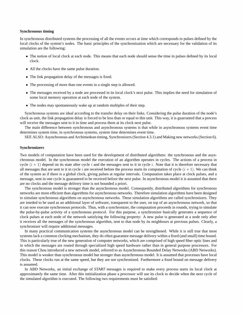
Synchronous timing
In synchronous distributed systems the processing of all the events occurs at time which corresponds to pulses defined by thelocal clocks of the system’s nodes. The basic principles of the synchronization which are necessary for the validation of itssimulation are the following:
• The notion of local clock at each node. This means that each node should sense the time in pulses defined by its localclock.
• All the clocks have the same pulse duration.
• The link propagation delay of the messages is fixed.
• The processing of more than one events in a single step is allowed.
• The messages received by a node are processed in its local clock’s next pulse. This implies the need for simulation ofsome local memory operation at each node of the system.
• The nodes may spontaneously wake up at random multiples of their step.
Synchronous systems are ideal according to the transfer delay on their links. Considering the pulse duration of the node’sclock as unit, the link propagation delay is forced to be less than or equal to this unit. This way, it is guarranted that a processwill receive the messages sent to it in time and process them at its clock next pulse.
The main difference between synchronous and asynchronous systems is that while in asynchronous systems event timedetermines system time, in synchronous systems, system time determines event time.
SEE ALSO: Asynchronous and Archimedean timing, Synchronizers (Section 4.3.1) and Making new networks (Section 6).
Synchronizers
Two models of computation have been used for the development of distributed algorithms: the synchronous and the asyn-chronous model. In the synchronous model the execution of an algorithm operates in cycles. The actions of a process incycle (i + 1) depend on its state after cyclei and the messages sent to it in cyclei. Note that it is therefore necessary thatall messages that are sent to it in cyclei are received before the process starts its computation of cycle(i + 1). We can thinkof the system as if there is a global clock, giving pulses at regular intervals. Computation takes place at clock pulses, and amessage, sent in one cycle is guaranteed to be received before the next pulse. In asynchronous model it is assumed that thereare no clocks and the message delivery time is not bounded a priori.
The synchronous model is stronger than the asynchronous model. Consequently, distributed algorithms for synchronousnetworks are more efficient than algorithms for asynchronous networks. Therefore simulation algorithms have been designedto simulate synchronous algorithms on asynchronous networks. These simulation algorithms are called synchronizers. Theyare inteded to be used as an additional layer of software, transparent to the user, on top of an asynchronous network, so thatit can now execute synchronous protocols. Thus, with a synchronizer, the computation proceeds in rounds, trying to simulatethe pulse-by-pulse activity of a synchronous protocol. For this purpose, a synchronizer basically generates a sequence ofclock pulses at each node of the network satisfying the following property: A new pulse is generated at a node only afterit receives all the messages of the synchronous algorithm, sent to that node by its neighbours at previous pulses. Clearly, asynchronizer will require additional messages.
In many practical communication systems the asynchronous model can be strengthened. While it is still true that mostsystems lack a common clocking mechanism, they do often guarantee message delivery within a fixed (and small) time bound.This is particularly true of the new generation of computer networks, which are comprised of high speed fiber optic lines andin which the messages are routed through specialized high speed hardware rather than in general purpose processors. Forthis reason Chou introduced a new network model, referred to as Asynchronous Bounded Delay Networks (ABD Networks).This model is weaker than synchronous model but stronger than asynchronous model. It is assumed that processes have localclocks. These clocks run at the same speed, but they are not synchronized. Furthermore a fixed bound on message deliveryis assumed.
In ABD Networks, an initial exchange ofSTART messages is required to make every process starts its local clock atapproximately the same time. After this intitialization phase a processor will use its clock to decide when the next cycle ofthe simulated algorithm is executed. The following two requirements must be satisfied:
R1 If a processq sends a message to its neighbourp in some cyclei, this message must be received beforep simulates cycle(i + 1); and
R2 if a processp receives a message it must be possible forp to determine to what cycle this message belongs.
Requirement R1 is obvious becausep’s actions in cycle(i + 1) depend onq’s message. Failure to meet the requirementR2 may lead to incorrect simulation.
To compare the speed of synchronizers on an ABD Network we introduce the concept of cycle time. The cycle time ofa synchronizer is the time it takes to simulate one cycle of the synchronous algorithm. Chou presented two synchronizers.His first synchronizer has a cycle time of 2. To meet the requirement R2, one bit is added to every message of the simulatedalgorithm. The synchronizer can be imlemented withO(1) storage per process.The extra bit is avoided in the second syn-chronizer, but this is paid for with a cycle time of 3. Tel,Zaks and Korach recently presented a synchronizer with a cycle timeof 2, without the extra bit. Internal storage needed in a node to implement this synchronizer equals the degree of the node onthe network. They also presented similar synchronizers for the more realistic case where the clocks may suffer a -small andbounded- drift.
SEE ALSO: Asynchronous and Archimedean timing, Synchronous timing (Section 4.3.1) and Making new networks(Section 6).
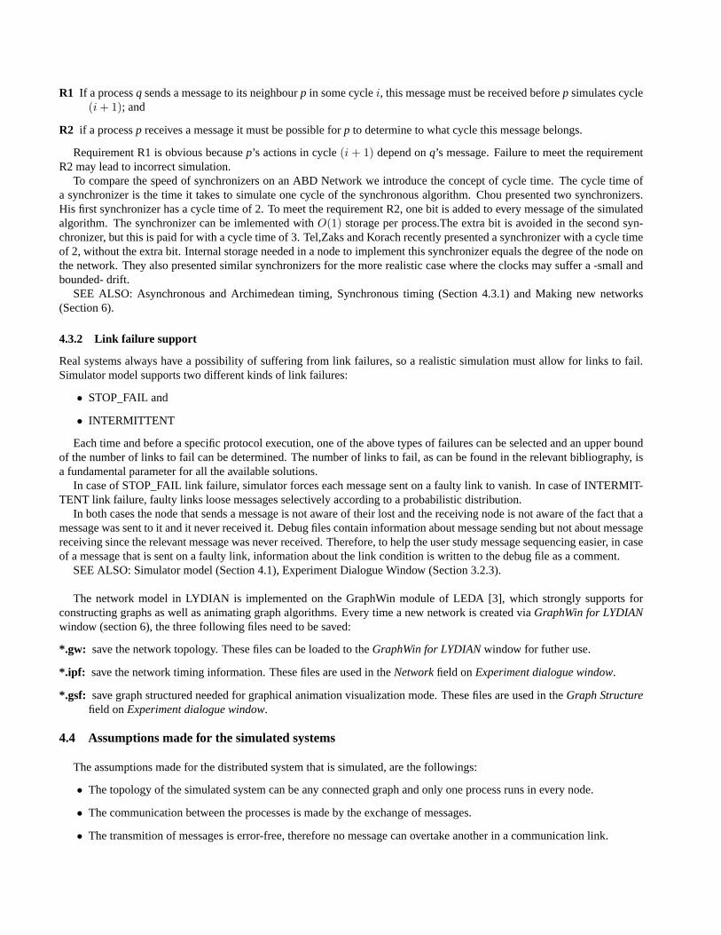
4.3.2 Link failure support
Real systems always have a possibility of suffering from link failures, so a realistic simulation must allow for links to fail.Simulator model supports two different kinds of link failures:
• STOP_FAIL and
• INTERMITTENT
Each time and before a specific protocol execution, one of the above types of failures can be selected and an upper boundof the number of links to fail can be determined. The number of links to fail, as can be found in the relevant bibliography, isa fundamental parameter for all the available solutions.
In case of STOP_FAIL link failure, simulator forces each message sent on a faulty link to vanish. In case of INTERMIT-TENT link failure, faulty links loose messages selectively according to a probabilistic distribution.
In both cases the node that sends a message is not aware of their lost and the receiving node is not aware of the fact that amessage was sent to it and it never received it. Debug files contain information about message sending but not about messagereceiving since the relevant message was never received. Therefore, to help the user study message sequencing easier, in caseof a message that is sent on a faulty link, information about the link condition is written to the debug file as a comment.
SEE ALSO: Simulator model (Section 4.1), Experiment Dialogue Window (Section 3.2.3).
The network model in LYDIAN is implemented on the GraphWin module of LEDA [3], which strongly supports forconstructing graphs as well as animating graph algorithms. Every time a new network is created viaGraphWin for LYDIANwindow (section 6), the three following files need to be saved:
*.gw: save the network topology. These files can be loaded to theGraphWin for LYDIAN window for futher use.
*.ipf: save the network timing information. These files are used in theNetwork field onExperiment dialogue window.
*.gsf: save graph structured needed for graphical animation visualization mode. These files are used in theGraph Structurefield onExperiment dialogue window.
4.4 Assumptions made for the simulated systems
The assumptions made for the distributed system that is simulated, are the followings:
• The topology of the simulated system can be any connected graph and only one process runs in every node.
• The communication between the processes is made by the exchange of messages.
• The transmition of messages is error-free, therefore no message can overtake another in a communication link.
• In every node only one event can happen at a time, therefore one message can be received at a time.
• The same protocol is running in every node and is called for execution every time an event occurs.
• The timing assumptions are flexible, so asynchronous, archimedean or synchronous protocols can be executed.
• Every node is initially in an idle state, calledSLEEPING, and begins to execute the protocol (wakes up) either sponta-neously (at a random time independent of the other nodes wake-up times in synchrony with the other nodes) or by thereceipt of a message (protocol dependent).
5 Making new protocols
As a way of illutrating how to make a new protocol we will go through the exercise creating a new protocol for algorithmBroadcast with ACK.
5.1 Design
From the algorithm, we need to identify how many external events can affect each process and how many states theprocess could have under these effects. For instance, the external events can be timeout interrupt or receiving a message, butnot sending a message. Then, we make a table where the rows and columns correspond to the external affecting events andthe states of the process, respectively.
state1 state2 ... staten
event1event2
...eventm
At the cell [eventi, statej ] the actions the process must do when its state isstatej and it is affected byeventi are filledin. The actions should be written in pseudo-code. After filling the table up, the algorithm becomes more clear to implement:each cell in the table is a procedure in the protocol source code. Of course, if two cells have the same content, only oneprocedure is enough. From the table, we can also identify how many local variables are necessary for each process.
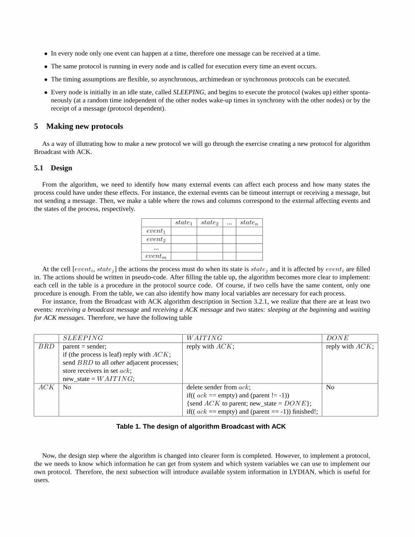
For instance, from the Broadcast with ACK algorithm description in Section 3.2.1, we realize that there are at least twoevents:receiving a broadcast message andreceiving a ACK message and two states:sleeping at the beginning andwaitingfor ACK messages. Therefore, we have the following table
SLEEPING WAITING DONEBRD parent = sender; reply withACK; reply withACK;
if (the process is leaf) reply withACK;sendBRD to all other adjacent processes;store receivers in setack;new_state =WAITING;
ACK No delete sender fromack; Noif(( ack == empty) and (parent != -1)){sendACK to parent; new_state =DONE};if(( ack == empty) and (parent == -1)) finished!;
Table 1. The design of algorithm Broadcast with ACK
Now, the design step where the algorithm is changed into clearer form is completed. However, to implement a protocol,the we needs to know which information he can get from system and which system variables we can use to implement ourown protocol. Therefore, the next subsection will introduce available system information in LYDIAN, which is useful forusers.
5.2 System structure
The system consists of processes -or nodes- arranged in a user specified topology. Each process may refer to its PCB(Process Control Block; see below in this section for the PCB structure) and its local variables. Global variables also existand can be accessed or not depending on the assumptions of the implemented protocol.
The communication among the processes is accomplished by exchanging messages. Each node has a number of portsequal to the number of its adjacent nodes. So each port is dedicated to one adjacent node. Each message is sent to andreceived from specified ports. The structure of the messages is standard.
The information about the number of processes, the system topology, the kind of timing, timing parameters is included innetwork description files and can change in different executions, as different networks are allowed to be used each time.
Note: The fields with (*) are often used by the user
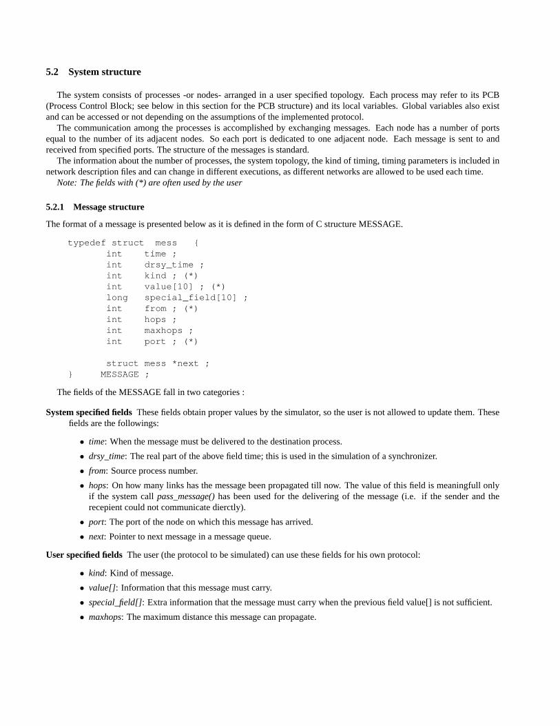
5.2.1 Message structure
The format of a message is presented below as it is defined in the form of C structure MESSAGE.
typedef struct mess {int time ;int drsy_time ;int kind ; (*)int value[10] ; (*)long special_field[10] ;int from ; (*)int hops ;int maxhops ;int port ; (*)
struct mess *next ;} MESSAGE ;
The fields of the MESSAGE fall in two categories :
System specified fieldsThese fields obtain proper values by the simulator, so the user is not allowed to update them. Thesefields are the followings:
• time: When the message must be delivered to the destination process.
• drsy_time: The real part of the above field time; this is used in the simulation of a synchronizer.
• from: Source process number.
• hops: On how many links has the message been propagated till now. The value of this field is meaningfull onlyif the system callpass_message() has been used for the delivering of the message (i.e. if the sender and therecepient could not communicate dierctly).
• port: The port of the node on which this message has arrived.
• next: Pointer to next message in a message queue.
User specified fieldsThe user (the protocol to be simulated) can use these fields for his own protocol:
• kind: Kind of message.
• value[]: Information that this message must carry.
• special_field[]: Extra information that the message must carry when the previous field value[] is not sufficient.
• maxhops: The maximum distance this message can propagate.
5.2.2 Node Process Control Block (PCB) and local variables
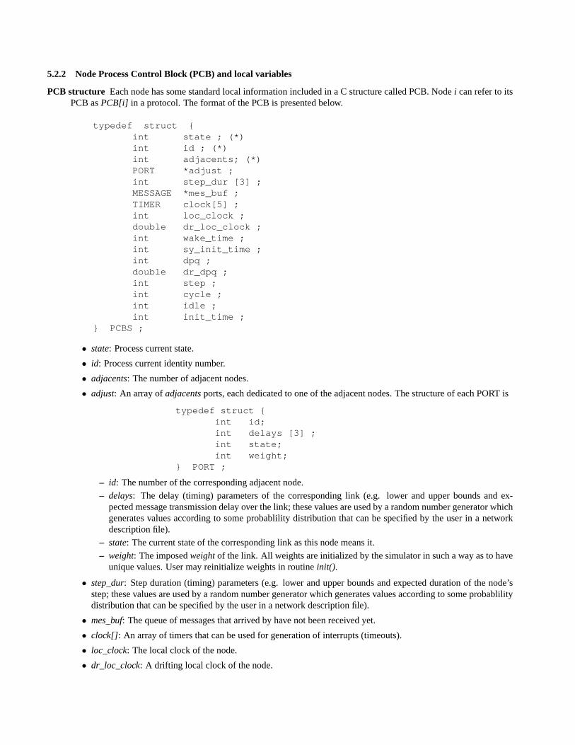
PCB structure Each node has some standard local information included in a C structure called PCB. Nodei can refer to itsPCB asPCB[i] in a protocol. The format of the PCB is presented below.
typedef struct {int state ; (*)int id ; (*)int adjacents; (*)PORT *adjust ;int step_dur [3] ;MESSAGE *mes_buf ;TIMER clock[5] ;int loc_clock ;double dr_loc_clock ;int wake_time ;int sy_init_time ;int dpq ;double dr_dpq ;int step ;int cycle ;int idle ;int init_time ;
} PCBS ;
• state: Process current state.
• id: Process current identity number.
• adjacents: The number of adjacent nodes.
• adjust: An array ofadjacents ports, each dedicated to one of the adjacent nodes. The structure of each PORT is
typedef struct {int id;int delays [3] ;int state;int weight;
} PORT ;
– id: The number of the corresponding adjacent node.
– delays: The delay (timing) parameters of the corresponding link (e.g. lower and upper bounds and ex-pected message transmission delay over the link; these values are used by a random number generator whichgenerates values according to some probablility distribution that can be specified by the user in a networkdescription file).
– state: The current state of the corresponding link as this node means it.
– weight: The imposedweight of the link. All weights are initialized by the simulator in such a way as to haveunique values. User may reinitialize weights in routineinit().
• step_dur: Step duration (timing) parameters (e.g. lower and upper bounds and expected duration of the node’sstep; these values are used by a random number generator which generates values according to some probablilitydistribution that can be specified by the user in a network description file).
• mes_buf: The queue of messages that arrived by have not been received yet.
• clock[]: An array of timers that can be used for generation of interrupts (timeouts).
• loc_clock: The local clock of the node.
• dr_loc_clock: A drifting local clock of the node.
• wake_time: This field keeps the time that the node’s local clock started to count.
• sy_init_time: Keeps the time that the node is going to wake up during the sychronizer’s initialization phase.
• dpq: The difference between the wake_times of two nodes p,q.
• dr_dpq: The difference between the wake_times of two nodes p,q when a synchronizer with drifting local clocksis simulated.
• step: Current step.
• cycle: Keeps the cycle of the local clock of the node.
• idle: Till when this node is idle.
• init_time: The time that a node is going to wake up.
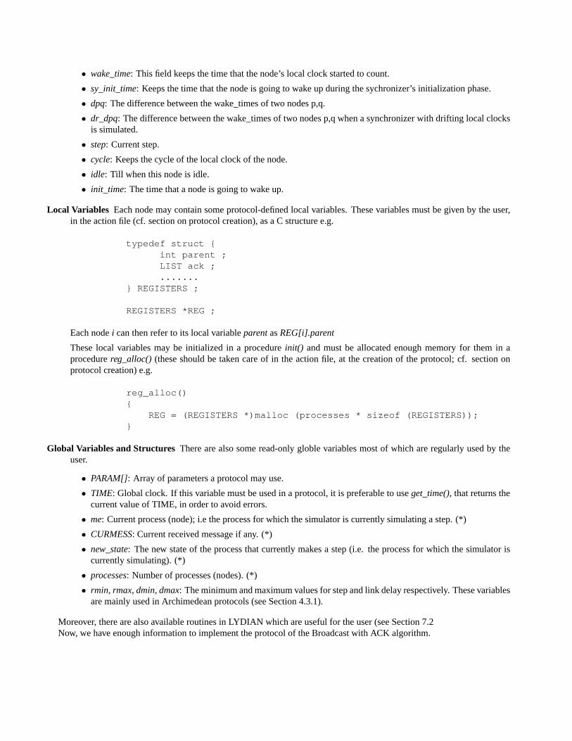
Local Variables Each node may contain some protocol-defined local variables. These variables must be given by the user,in the action file (cf. section on protocol creation), as a C structure e.g.
typedef struct {int parent ;LIST ack ;.......
} REGISTERS ;
REGISTERS *REG ;
Each nodei can then refer to its local variableparent asREG[i].parent
These local variables may be initialized in a procedureinit() and must be allocated enough memory for them in aprocedurereg_alloc() (these should be taken care of in the action file, at the creation of the protocol; cf. section onprotocol creation) e.g.
reg_alloc(){
REG = (REGISTERS *)malloc (processes * sizeof (REGISTERS));}
Global Variables and Structures There are also some read-only globle variables most of which are regularly used by theuser.
• PARAM[]: Array of parameters a protocol may use.
• TIME: Global clock. If this variable must be used in a protocol, it is preferable to useget_time(), that returns thecurrent value of TIME, in order to avoid errors.
• me: Current process (node); i.e the process for which the simulator is currently simulating a step. (*)
• CURMESS: Current received message if any. (*)
• new_state: The new state of the process that currently makes a step (i.e. the process for which the simulator iscurrently simulating). (*)
• processes: Number of processes (nodes). (*)
• rmin, rmax, dmin, dmax: The minimum and maximum values for step and link delay respectively. These variablesare mainly used in Archimedean protocols (see Section 4.3.1).
Moreover, there are also available routines in LYDIAN which are useful for the user (see Section 7.2Now, we have enough information to implement the protocol of the Broadcast with ACK algorithm.
typedef struct {/* all local variables must be declared here */...} REGISTERS;
REGISTERS ∗ REG;
reg_alloc() {REG = (REGISTERS∗)malloc(processes∗sizeof(REGISTERS));
}
init() {/* all local variables must be initilaized here */...
}
/* Below are your own procedures */...
Figure 13. The framework of protocol source code
typedef struct {int parent;LIST ack;} REGISTERS;
REGISTERS ∗ REG;
reg_alloc() {REG = (REGISTERS∗)malloc(processes∗sizeof(REGISTERS));
}
init() {for(i = 0; i < processes; i + +) {
REG[i].parent = −1;init_list(REG[i].ack);
}}
Figure 14. Initialization part of protocol Broadcast with ACK
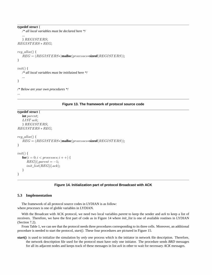
5.3 Implementation
The framework of all protocol source codes in LYDIAN is as follow:whereprocesses is one of globle variables in LYDIAN.
With the Broadcast with ACK protocol, we need two local variablesparent to keep the sender andack to keep a list ofreceivers. Therefore, we have the first part of code as in Figure 14 whereinit_list is one of available routines in LYDIAN(Section 7.2).
From Table 1, we can see that the protocol needs three procedures corresponding to its three cells. Moreover, an additionalprocedure is needed to start the protocol,start(). These four procedures are pictured in Figure 15.
start() is used to initialize the simulation byonly one process which is the initiator in network file description. Therefore,the network descritption file used for the protocol must have only one initiator. The procedure sendsBRD messagesfor all its adjacent nodes and keeps track of these messages in listack in other to wait for necessaryACK messages.
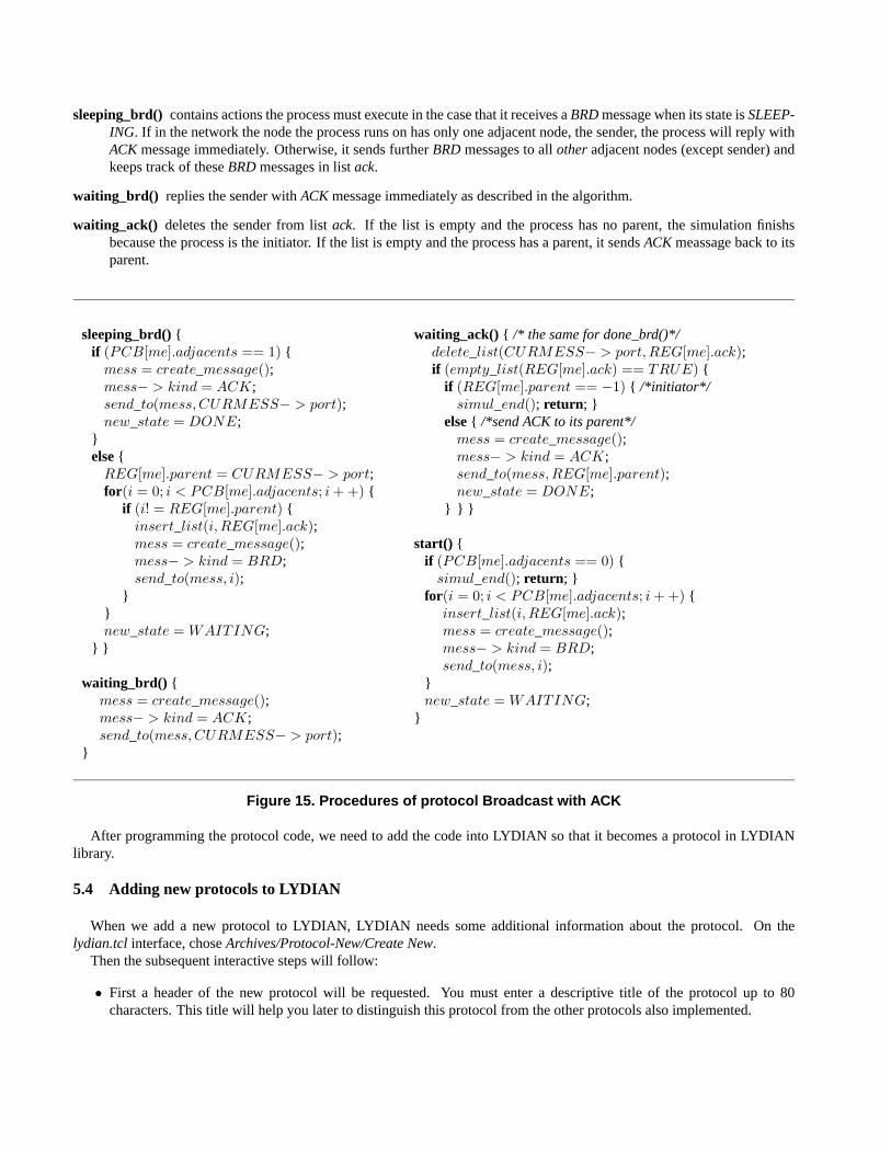
sleeping_brd() contains actions the process must execute in the case that it receives aBRD message when its state isSLEEP-ING. If in the network the node the process runs on has only one adjacent node, the sender, the process will reply withACK message immediately. Otherwise, it sends furtherBRD messages to allother adjacent nodes (except sender) andkeeps track of theseBRD messages in listack.
waiting_brd() replies the sender withACK message immediately as described in the algorithm.
waiting_ack() deletes the sender from listack. If the list is empty and the process has no parent, the simulation finishsbecause the process is the initiator. If the list is empty and the process has a parent, it sendsACK meassage back to itsparent.
sleeping_brd(){if (PCB[me].adjacents == 1) {
mess = create_message();mess− > kind = ACK;send_to(mess,CURMESS− > port);new_state = DONE;
}else{
REG[me].parent = CURMESS− > port;for(i = 0; i < PCB[me].adjacents; i + +) {
if (i! = REG[me].parent) {insert_list(i, REG[me].ack);mess = create_message();mess− > kind = BRD;send_to(mess, i);
}}new_state = WAITING;
} }
waiting_brd() {mess = create_message();mess− > kind = ACK;send_to(mess,CURMESS− > port);
}
waiting_ack() { /* the same for done_brd()*/delete_list(CURMESS− > port,REG[me].ack);if (empty_list(REG[me].ack) == TRUE) {
if (REG[me].parent == −1) { /*initiator*/simul_end(); return ; }
else{ /*send ACK to its parent*/mess = create_message();mess− > kind = ACK;send_to(mess,REG[me].parent);new_state = DONE;
} } }
start() {if (PCB[me].adjacents == 0) {
simul_end(); return ; }for(i = 0; i < PCB[me].adjacents; i + +) {
insert_list(i, REG[me].ack);mess = create_message();mess− > kind = BRD;send_to(mess, i);
}new_state = WAITING;
}
Figure 15. Procedures of protocol Broadcast with ACK
After programming the protocol code, we need to add the code into LYDIAN so that it becomes a protocol in LYDIANlibrary.
5.4 Adding new protocols to LYDIAN
When we add a new protocol to LYDIAN, LYDIAN needs some additional information about the protocol. On thelydian.tcl interface, choseArchives/Protocol-New/Create New.
Then the subsequent interactive steps will follow:
• First a header of the new protocol will be requested. You must enter a descriptive title of the protocol up to 80characters. This title will help you later to distinguish this protocol from the other protocols also implemented.
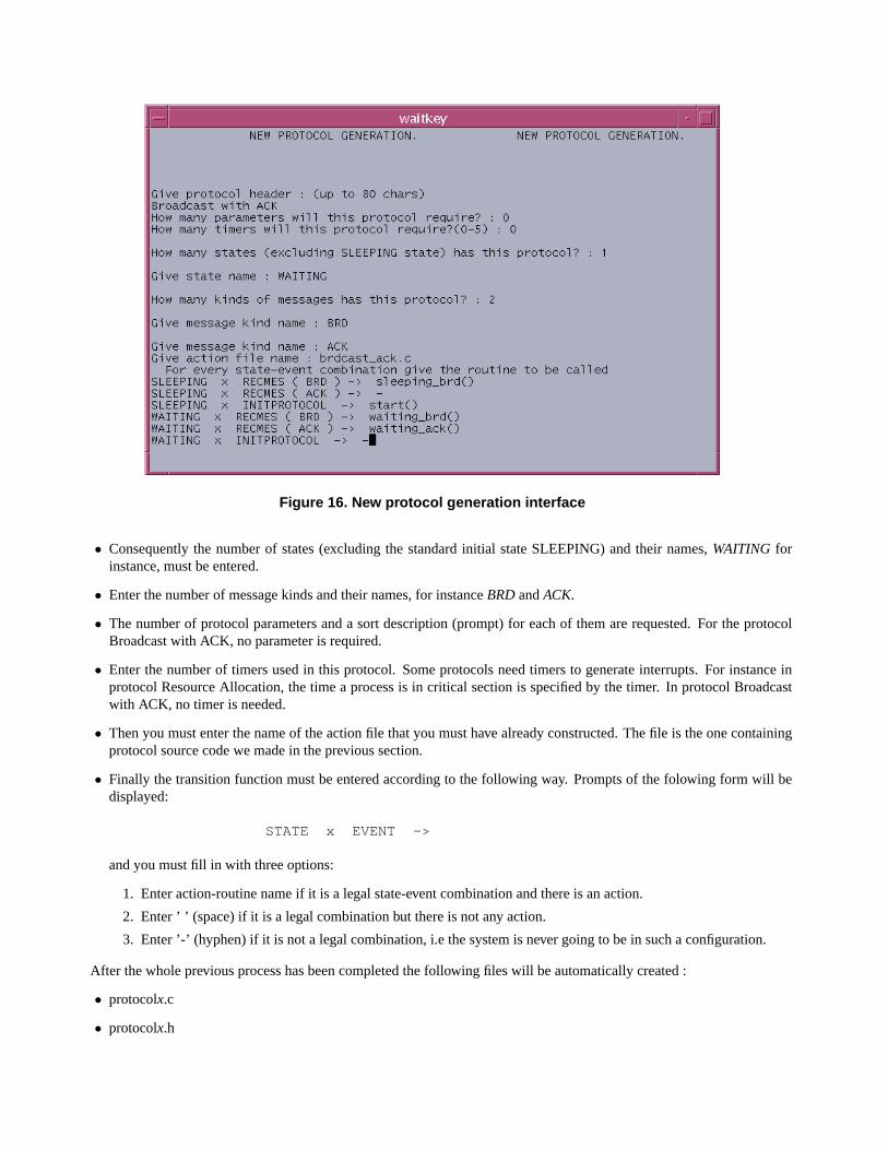
Figure 16. New protocol generation interface
• Consequently the number of states (excluding the standard initial state SLEEPING) and their names,WAITING forinstance, must be entered.
• Enter the number of message kinds and their names, for instanceBRD andACK.
• The number of protocol parameters and a sort description (prompt) for each of them are requested. For the protocolBroadcast with ACK, no parameter is required.
• Enter the number of timers used in this protocol. Some protocols need timers to generate interrupts. For instance inprotocol Resource Allocation, the time a process is in critical section is specified by the timer. In protocol Broadcastwith ACK, no timer is needed.
• Then you must enter the name of the action file that you must have already constructed. The file is the one containingprotocol source code we made in the previous section.
• Finally the transition function must be entered according to the following way. Prompts of the folowing form will bedisplayed:
STATE x EVENT ->
and you must fill in with three options:
1. Enter action-routine name if it is a legal state-event combination and there is an action.
2. Enter ’ ’ (space) if it is a legal combination but there is not any action.
3. Enter ’-’ (hyphen) if it is not a legal combination, i.e the system is never going to be in such a configuration.
After the whole previous process has been completed the following files will be automatically created :
• protocolx.c
• protocolx.h
• namesx
wherex is the number of the protocol. The protocol also has been inserted in the simulator catalog. So the new protocol iscompiled and is linked to the simulator. If errors occur during this phase you must select theArchives/Protocol-Edit fromlydian.tcl in order to correct possible typing or logic errors inprotocolx.c. Then choseArchives/Protocol-New/Import toimport the corrected protocol. To know how to debug a protocol source code, see Section 7.1 and Section 7.2.4
After succesful compilation and linking of the new protocol it is able to run on the simulator.For more information about the protocol model in LYDIAN, see Section 4.2.
6 Making new networks
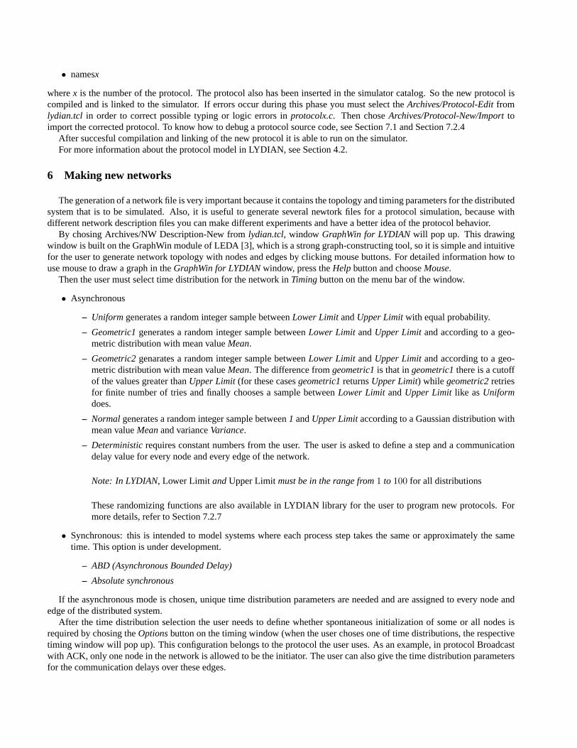
The generation of a network file is very important because it contains the topology and timing parameters for the distributedsystem that is to be simulated. Also, it is useful to generate several newtork files for a protocol simulation, because withdifferent network description files you can make different experiments and have a better idea of the protocol behavior.
By chosing Archives/NW Description-New fromlydian.tcl, window GraphWin for LYDIAN will pop up. This drawingwindow is built on the GraphWin module of LEDA [3], which is a strong graph-constructing tool, so it is simple and intuitivefor the user to generate network topology with nodes and edges by clicking mouse buttons. For detailed information how touse mouse to draw a graph in theGraphWin for LYDIAN window, press theHelp button and chooseMouse.
Then the user must select time distribution for the network inTiming button on the menu bar of the window.
• Asynchronous
– Uniform generates a random integer sample betweenLower Limit andUpper Limit with equal probability.
– Geometric1 generates a random integer sample betweenLower Limit andUpper Limit and according to a geo-metric distribution with mean valueMean.
– Geometric2 genarates a random integer sample betweenLower Limit andUpper Limit and according to a geo-metric distribution with mean valueMean. The difference fromgeometric1 is that ingeometric1 there is a cutoffof the values greater thanUpper Limit (for these casesgeometric1 returnsUpper Limit) while geometric2 retriesfor finite number of tries and finally chooses a sample betweenLower Limit andUpper Limit like asUniformdoes.
– Normal generates a random integer sample between1 andUpper Limit according to a Gaussian distribution withmean valueMean and varianceVariance.
– Deterministic requires constant numbers from the user. The user is asked to define a step and a communicationdelay value for every node and every edge of the network.
Note: In LYDIAN, Lower Limit and Upper Limit must be in the range from 1 to 100 for all distributions
These randomizing functions are also available in LYDIAN library for the user to program new protocols. Formore details, refer to Section 7.2.7
• Synchronous: this is intended to model systems where each process step takes the same or approximately the sametime. This option is under development.
– ABD (Asynchronous Bounded Delay)
– Absolute synchronous
If the asynchronous mode is chosen, unique time distribution parameters are needed and are assigned to every node andedge of the distributed system.
After the time distribution selection the user needs to define whether spontaneous initialization of some or all nodes isrequired by chosing theOptions button on the timing window (when the user choses one of time distributions, the respectivetiming window will pop up). This configuration belongs to the protocol the user uses. As an example, in protocol Broadcastwith ACK, only one node in the network is allowed to be the initiator. The user can also give the time distribution parametersfor the communication delays over these edges.
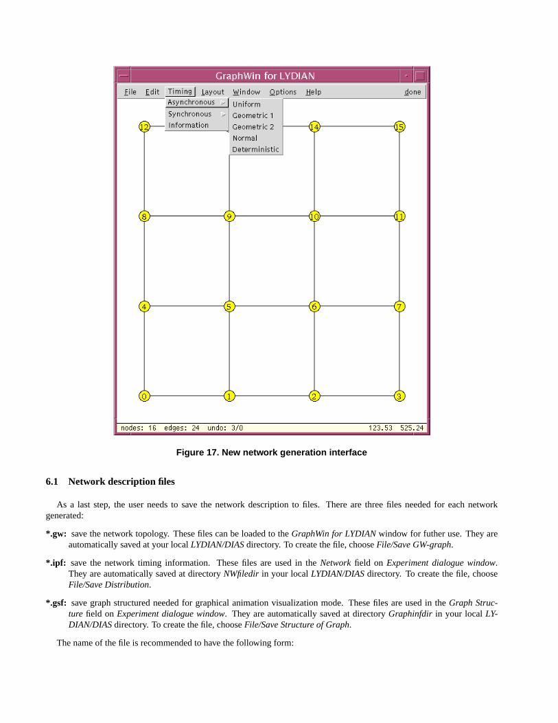
Figure 17. New network generation interface
6.1 Network description files
As a last step, the user needs to save the network description to files. There are three files needed for each networkgenerated:
*.gw: save the network topology. These files can be loaded to theGraphWin for LYDIAN window for futher use. They areautomatically saved at your localLYDIAN/DIAS directory. To create the file, chooseFile/Save GW-graph.
*.ipf: save the network timing information. These files are used in theNetwork field on Experiment dialogue window.They are automatically saved at directoryNWfiledir in your localLYDIAN/DIAS directory. To create the file, chooseFile/Save Distribution.
*.gsf: save graph structured needed for graphical animation visualization mode. These files are used in theGraph Struc-ture field on Experiment dialogue window. They are automatically saved at directoryGraphinfdir in your localLY-DIAN/DIAS directory. To create the file, chooseFile/Save Structure of Graph.
The name of the file is recommended to have the following form:
<topology name>_<time distribution name>_<number of nodes>
The suggested names of distribution choices are :
• For Uniform: “un”.
• For Geometric1: “g1".
• For Geometric2: “g2".
• For Normal: “nr".
• For Deterministic: “de".
• For User defined: “ud".
• For Synchronous: “sy".
• For ABD: “ab".
7 DIAS reference
The distributed systems simulator of Lydian is based on the simulator of the DSS tool [4].
7.1 Debugging and metrics
Besides the main display interface, there is another option for debugging and tracing an execution, by means of a debug(trace) file that is created for every execution of the simulator. In this file some information about the execution is printedand is available for off-line checking or any other use. If no debug-file-name is otherwise specified, the default name has theform:
debug.protocol number.process-id of simulator executionThe debug file consists of three parts: the header lines, the execution tracing part and the footer part.
7.1.1 Header
The header contains the debug file name, the name of the protocol that was executed and the name of the network descriptionfile that was selected. It also gives some system information of the terminal status before and during the protocol execution.If some kind of link failure is simulated, the type of the failure and the upper bound of the number of links to fail are alsogiven. In case of use of an ABD synchronizer with drifting clocks, the drift bound is given as well.
7.1.2 Tracing part
At this part, depending on what debug options were chosen, for every step of execution, information about the transition isprinted. The debug options available and the corresponding classes of information are:
a the state transition, current event and messages sentd the random samples chosen for processes steps and message transmission delayse event statust timer statusp protocol-defined tracing information; this information can be printed by invocation
of the proceduredebug(“p", “message ", args) by the protocol.s if multiple executions of a protocol are run in one simulation invocation, this debug
option chooses to also get the information on the mean numbers together with thesize of the topology are added in filestimes.protocol_number andmess.protocol_number(subdirectory/stats)
g if the visual output display interface is disabled, this option directs thedebug-file-information to the screen (standard output).
7.1.3 Footer
After the termination of an execution, the total time duration and number of messages sent is printed, together with systeminformation about the blocks of storage that remain allocated.
In the case of multiple executions, after all the executions have completed, the mean numbers and the distributions areprinted. If the-s option is chosen the mean numbers together with the size of the topology are added in filestimes.protocol_numberandmess.protocol_number that are in the subdirectory/stats.
The structure of this file is made for convenient use with programs that make graphical reperesentations of the results,such as GRAPHER.
SEE ALSO: Debugging and User Interface routines, meas.h.
7.2 Available routines in the simulator
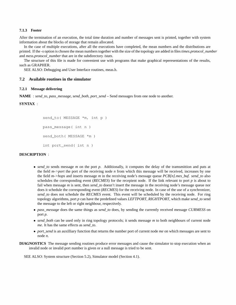
7.2.1 Message delivering
NAME : send_to, pass_message, send_both, port_send – Send messages from one node to another.
SYNTAX :
send_to( MESSAGE *m, int p )
pass_message( int n )
send_both( MESSAGE *m )
int port_send( int n )
DESCRIPTION :
• send_to sends messagem on the portp. Additionally, it computes the delay of the tramsmittion and puts atthe fieldm->port the port of the receiving noden from which this message will be received, increases by onethe fieldm->hops and inserts messagem in the receiving node’s message queuePCB[n].mes_buf. send_to alsoschedules the corresponding event (RECMES) for the recepient node. If the link relevant to portp is about tofail when messagem is sent, thensend_to doesn’t insert the message in the receiving node’s message queue nordoes it schedule the corresponding event (RECMES) for the receiving node. In case of the use of a synchronizer,send_to does not schedule theRECMES event. This event will be scheduled by the receiving node. For ringtopology algorithms, portp can have the predefined valuesLEFTPORT, RIGHTPORT, which makesend_to sendthe message to the left or right neighbour, respectively.
• pass_message does the same things assend_to does, by sending the currently received messageCURMESS onport p.
• send_both can be used only in ring topology protocols; it sends messagem to both neighbours of current nodeme. It has the same effects assend_to.
• port_send is an auxilliary function that returns the number port of current nodeme on which messages are sent tonoden.
DIAGNOSTICS The message sending routines produce error messages and cause the simulator to stop execution when aninvalid node or invalid port number is given or a null message is tried to be sent.
SEE ALSO: System structure (Section 5.2), Simulator model (Section 4.1).
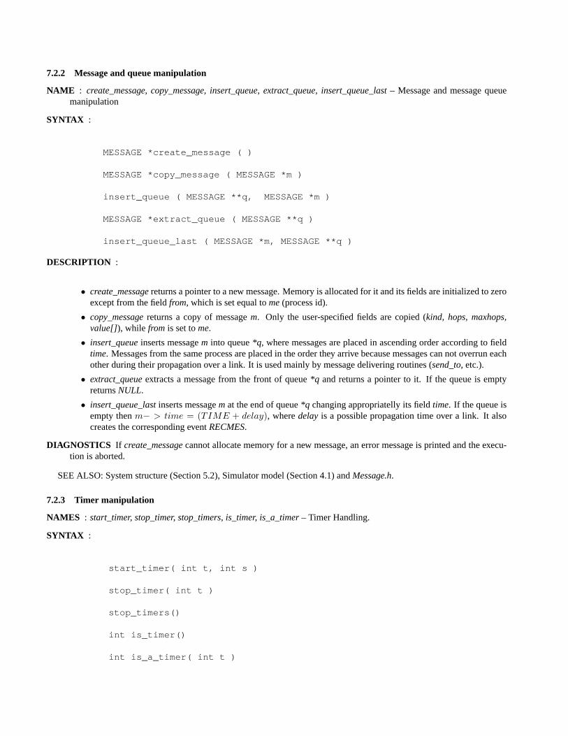
7.2.2 Message and queue manipulation
NAME : create_message, copy_message, insert_queue, extract_queue, insert_queue_last – Message and message queuemanipulation
SYNTAX :
MESSAGE *create_message ( )
MESSAGE *copy_message ( MESSAGE *m )
insert_queue ( MESSAGE **q, MESSAGE *m )
MESSAGE *extract_queue ( MESSAGE **q )
insert_queue_last ( MESSAGE *m, MESSAGE **q )
DESCRIPTION :
• create_message returns a pointer to a new message. Memory is allocated for it and its fields are initialized to zeroexcept from the fieldfrom, which is set equal tome (process id).
• copy_message returns a copy of messagem. Only the user-specified fields are copied (kind, hops, maxhops,value[]), while from is set tome.
• insert_queue inserts messagem into queue*q, where messages are placed in ascending order according to fieldtime. Messages from the same process are placed in the order they arrive because messages can not overrun eachother during their propagation over a link. It is used mainly by message delivering routines (send_to, etc.).
• extract_queue extracts a message from the front of queue*q and returns a pointer to it. If the queue is emptyreturnsNULL.
• insert_queue_last inserts messagem at the end of queue*q changing appropriatelly its fieldtime. If the queue isempty thenm− > time = (TIME + delay), wheredelay is a possible propagation time over a link. It alsocreates the corresponding eventRECMES.
DIAGNOSTICS If create_message cannot allocate memory for a new message, an error message is printed and the execu-tion is aborted.
SEE ALSO: System structure (Section 5.2), Simulator model (Section 4.1) andMessage.h.
7.2.3 Timer manipulation
NAMES : start_timer, stop_timer, stop_timers, is_timer, is_a_timer – Timer Handling.
SYNTAX :
start_timer( int t, int s )
stop_timer( int t )
stop_timers()
int is_timer()
int is_a_timer( int t )
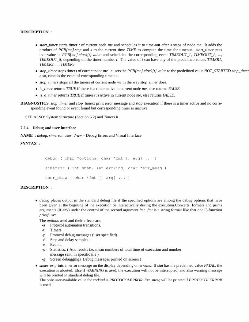
DESCRIPTION :
• start_timer starts timert of current nodeme and schedules it to time-out afters steps of nodeme. It adds theproduct ofPCB[me].step and s to the current timeTIME to compute the time for timeout.start_timer putsthat value inPCB[me].clock[t].value and schedules the corresponding eventTIMEOUT_1, TIMEOUT_2, ...,TIMEOUT_5, depending on the timer numbert. The value oft can have any of the predefined valuesTIMER1,TIMER2, ..., TIMER5.
• stop_timer stops timert of current nodeme i.e. sets thePCB[me].clock[t].value to the predefined valueNOT_STARTED.stop_timeralso, cancels the event of corresponding timeout.
• stop_timers stops all the timers of current nodeme in the waystop_timer does.
• is_timer returnsTRUE if there is a timer active in current nodeme, else returnsFALSE.
• is_a_timer returnsTRUE if timer t is active in current nodeme, else returnsFALSE.
DIAGNOSTICS stop_timer andstop_timers print error message and stop execution if there is a timer active and no corre-sponding event found or event found but corresponding timer is inactive.
SEE ALSO: System Structure (Section 5.2) andTimers.h.
7.2.4 Debug and user interface
NAME : debug, simerror, user_draw – Debug Errors and Visual Interface
SYNTAX :
debug ( char *options, char *fmt [, arg] ... )
simerror ( int stat, int errkind, char *err_mesg )
user_draw ( char *fmt [, arg] ... )
DESCRIPTION :
• debug places output in the standard debug file if the specified options are among the debug options that havebeen given at the begining of the execution or interactivelly during the execution.Converts, formats and printsarguments (if any) under the control of the second argumentfmt. fmt is a string format like that one C-functionprintf uses.
Theoptions used and their effects are:-a Protocol automaton transitions.-t Timers.-p Protocol debug messages (user specified).-d Step and delay samples.-e Events.-s Statistics. ( Add results i.e. mean numbers of total time of execution and number
message sent, in specific file )-g Screen debugging.( Debug messages printed on screen )
• simerror prints an error message on the display depending onerrkind. If stat has the predefined valueFATAL, theexecution is aborted. Else ifWARNING is used, the execution will not be interrupted, and also warning messagewill be printed in standard debug file.The only user available value forerrkind is PROTOCOLERROR. Err_mesg will be printed ifPROTOCOLERRORis used.
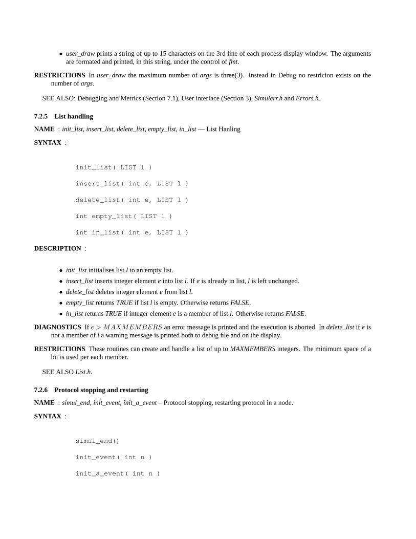
• user_draw prints a string of up to 15 characters on the 3rd line of each process display window. The argumentsare formated and printed, in this string, under the control offmt.
RESTRICTIONS In user_draw the maximum number ofargs is three(3). Instead in Debug no restricion exists on thenumber ofargs.
SEE ALSO: Debugging and Metrics (Section 7.1), User interface (Section 3),Simulerr.h andErrors.h.
7.2.5 List handling
NAME : init_list, insert_list, delete_list, empty_list, in_list — List Hanling
SYNTAX :
init_list( LIST l )
insert_list( int e, LIST l )
delete_list( int e, LIST l )
int empty_list( LIST l )
int in_list( int e, LIST l )
DESCRIPTION :
• init_list initialises listl to an empty list.
• insert_list inserts integer elemente into list l. If e is already in list,l is left unchanged.
• delete_list deletes integer elemente from list l.
• empty_list returnsTRUE if list l is empty. Otherwise returnsFALSE.
• in_list returnsTRUE if integer elemente is a member of listl. Otherwise returnsFALSE.
DIAGNOSTICS If e > MAXMEMBERS an error message is printed and the execution is aborted. Indelete_list if e isnot a member ofl a warning message is printed both to debug file and on the display.
RESTRICTIONS These routines can create and handle a list of up toMAXMEMBERS integers. The minimum space of abit is used per each member.
SEE ALSOList.h.
7.2.6 Protocol stopping and restarting
NAME : simul_end, init_event, init_a_event – Protocol stopping, restarting protocol in a node.
SYNTAX :
simul_end()
init_event( int n )
init_a_event( int n )
DESCRIPTION :
• simul_end can be called from protocol when a node decides that the execution must be ended. It must be in everyprotocol implementation, because it is the only succesful way of ending the protocol execution. When it is calledfrom a node all pending events are not executed and simulator displays the messageThis is the END !.
• init_event creates the initializing eventINITPROTOCOL and schedules it to be executed after a delay uniformlydistributed between the initial starting time limitsmin_init_time andmax_init_time that take their values frominput file.
• init_a_event creates the initializing eventINITPROTOCOL and schedules it to be executed at the user specifiedtime that is indicated by fieldPCB[i].init_time. In case of the use of a synchronizer,PCB[i].wake_time is alsoconsidered in the evaluation of the time that theINITPROTOCOL event is going to happen.
SEE ALSO: System structure (Section 5.2) andSimul.h.
7.2.7 Randomizing
NAME : randomize, uniform, geometric1, geometric2, normal, randfunc – Randomizing routines
SYNTAX :
int randomize ( int x[3] )
int uniform ( int l, int u )
int geometric1 ( int l, int u, int m )
int geometric2 ( int l, int u, int m )
normal ( int m, int u, int v )
float randfunc ()
DESCRIPTION :These routines use the system function random in order to produce a random number according to a specific probabilitydistribution function.
• randomize returns a step or delay sample according to the time distribution function used at the specific executionand recorded to the global variableTIMEDISTR, and also the argument arrayx which contains the parame-ters of the distribution function. So in order to obtain a step sample for processi you can write:step_sample =randomize(PCB[i].step_dur) and for a delay sample for processi and portj: delay_sample = randomize(PCB[i].adjust[j].
• uniform returns a random integer sample betweenl andu with equal probability.
• geometric1 returns a random integer sample betweenl andu and according to a geometric distribution with meanvaluem.
• geometric2 returns a random integer sample betweenl andu and according to a geometric distribution with meanvaluem. The difference fromgeometric1 is that ingeometric1 there is a cutoff of the values greater thanu (forthese casesgeometric1 returnsu) while geometric2 retries for finite number of tries and finally chooses a samlebetweenl andu like asuniform does.
• normal returns a random integer sample between1 andu according to a Gaussian distribution with mean valuemand variancev.
• randfunc returns a random real sample between0 and1 according to a uniform distribution.
SEE ALSO: Flexible Timing Assumptions (Section 4.3.1), System structure (Section 5.2) andDistr.h.
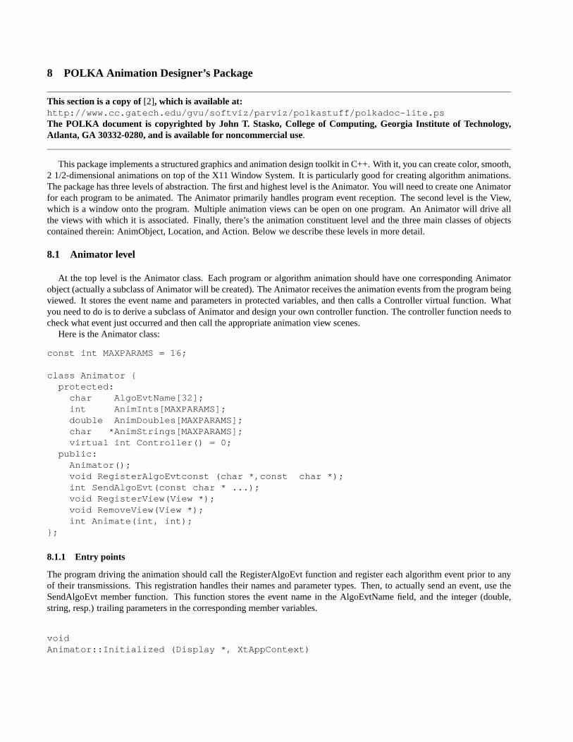
8 POLKA Animation Designer’s Package
This section is a copy of[2], which is available at:http://www.cc.gatech.edu/gvu/softviz/parviz/polkastuff/polkadoc-lite.psThe POLKA document is copyrighted by John T. Stasko, College of Computing, Georgia Institute of Technology,Atlanta, GA 30332-0280, and is available for noncommercial use.
This package implements a structured graphics and animation design toolkit in C++. With it, you can create color, smooth,2 1/2-dimensional animations on top of the X11 Window System. It is particularly good for creating algorithm animations.The package has three levels of abstraction. The first and highest level is the Animator. You will need to create one Animatorfor each program to be animated. The Animator primarily handles program event reception. The second level is the View,which is a window onto the program. Multiple animation views can be open on one program. An Animator will drive allthe views with which it is associated. Finally, there’s the animation constituent level and the three main classes of objectscontained therein: AnimObject, Location, and Action. Below we describe these levels in more detail.
8.1 Animator level
At the top level is the Animator class. Each program or algorithm animation should have one corresponding Animatorobject (actually a subclass of Animator will be created). The Animator receives the animation events from the program beingviewed. It stores the event name and parameters in protected variables, and then calls a Controller virtual function. Whatyou need to do is to derive a subclass of Animator and design your own controller function. The controller function needs tocheck what event just occurred and then call the appropriate animation view scenes.
Here is the Animator class:
const int MAXPARAMS = 16;
class Animator {protected:
char AlgoEvtName[32];int AnimInts[MAXPARAMS];double AnimDoubles[MAXPARAMS];char *AnimStrings[MAXPARAMS];virtual int Controller() = 0;
public:Animator();void RegisterAlgoEvtconst (char *,const char *);int SendAlgoEvt(const char * ...);void RegisterView(View *);void RemoveView(View *);int Animate(int, int);
};
8.1.1 Entry points
The program driving the animation should call the RegisterAlgoEvt function and register each algorithm event prior to anyof their transmissions. This registration handles their names and parameter types. Then, to actually send an event, use theSendAlgoEvt member function. This function stores the event name in the AlgoEvtName field, and the integer (double,string, resp.) trailing parameters in the corresponding member variables.
voidAnimator::Initialized (Display *, XtAppContext)
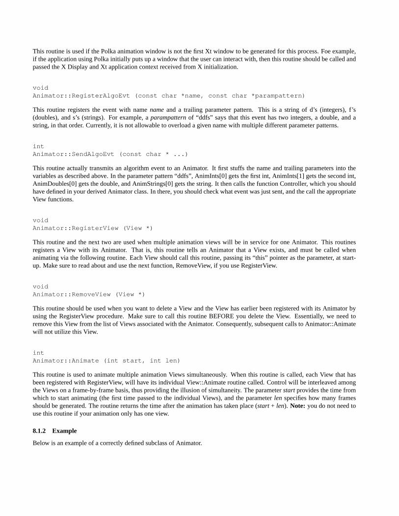
This routine is used if the Polka animation window is not the first Xt window to be generated for this process. Foe example,if the application using Polka initially puts up a window that the user can interact with, then this routine should be called andpassed the X Display and Xt application context received from X initialization.
voidAnimator::RegisterAlgoEvt (const char *name, const char *parampattern)
This routine registers the event with namename and a trailing parameter pattern. This is a string of d’s (integers), f’s(doubles), and s’s (strings). For example, aparampattern of “ddfs” says that this event has two integers, a double, and astring, in that order. Currently, it is not allowable to overload a given name with multiple different parameter patterns.
intAnimator::SendAlgoEvt (const char * ...)
This routine actually transmits an algorithm event to an Animator. It first stuffs the name and trailing parameters into thevariables as described above. In the parameter pattern “ddfs”, AnimInts[0] gets the first int, AnimInts[1] gets the second int,AnimDoubles[0] gets the double, and AnimStrings[0] gets the string. It then calls the function Controller, which you shouldhave defined in your derived Animator class. In there, you should check what event was just sent, and the call the appropriateView functions.
voidAnimator::RegisterView (View *)
This routine and the next two are used when multiple animation views will be in service for one Animator. This routinesregisters a View with its Animator. That is, this routine tells an Animator that a View exists, and must be called whenanimating via the following routine. Each View should call this routine, passing its “this” pointer as the parameter, at start-up. Make sure to read about and use the next function, RemoveView, if you use RegisterView.
voidAnimator::RemoveView (View *)
This routine should be used when you want to delete a View and the View has earlier been registered with its Animator byusing the RegisterView procedure. Make sure to call this routine BEFORE you delete the View. Essentially, we need toremove this View from the list of Views associated with the Animator. Consequently, subsequent calls to Animator::Animatewill not utilize this View.
intAnimator::Animate (int start, int len)
This routine is used to animate multiple animation Views simultaneously. When this routine is called, each View that hasbeen registered with RegisterView, will have its individual View::Animate routine called. Control will be interleaved amongthe Views on a frame-by-frame basis, thus providing the illusion of simultaneity. The parameterstart provides the time fromwhich to start animating (the first time passed to the individual Views), and the parameterlen specifies how many framesshould be generated. The routine returns the time after the animation has taken place (start + len). Note: you do not need touse this routine if your animation only has one view.
8.1.2 Example
Below is an example of a correctly defined subclass of Animator.
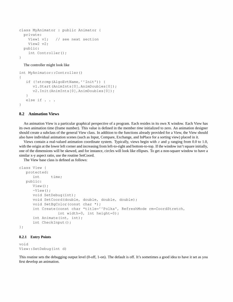
class MyAnimator : public Animator {private:
View1 v1; // see next sectionView2 v2;
public:int Controller();
}
The controller might look like
int MyAnimator::Controller(){
if (!strcmp(AlgoEvtName,’’Init")) {v1.Start(AnimInts[0],AnimDoubles[0]);v2.Init(AnimInts[0],AnimDoubles[0]);
}else if . . .
}
8.2 Animation Views
An animation View is a particular graphical perspective of a program. Each resides in its own X window. Each View hasits own animation time (frame number). This value is defined in the membertime initialized to zero. An animation designershould create a subclass of the general View class. In addition to the functions already provided for a View, the View shouldalso have individual animation scenes (such as Input, Compare, Exchange, and InPlace for a sorting view) placed in it.
Views contain a real-valued animation coordinate system. Typically, views begin withx andy ranging from 0.0 to 1.0,with the origin at the lower left corner and increasing from left-to-right and bottom-to-top. If the window isn’t square initially,one of the dimensions will be skewed, and for instance, circles will look like ellipses. To get a non-square window to have asimilar x-y aspect ratio, use the routine SetCoord.
The View base class is defined as follows:
class View {protected:
int time;public:
View();~View();void SetDebug(int);void SetCoord(double, double, double, double);void SetBgColor(const char *);int Create(const char *title=’’Polka", RefreshMode rm=CoordStretch,
int width=0, int height=0);int Animate(int, int);int CheckInput();
};
8.2.1 Entry Points
voidView::SetDebug(int d)
This routine sets the debugging output level (0-off, 1-on). The default is off. It’s sometimes a good idea to have it set as youfirst develop an animation.
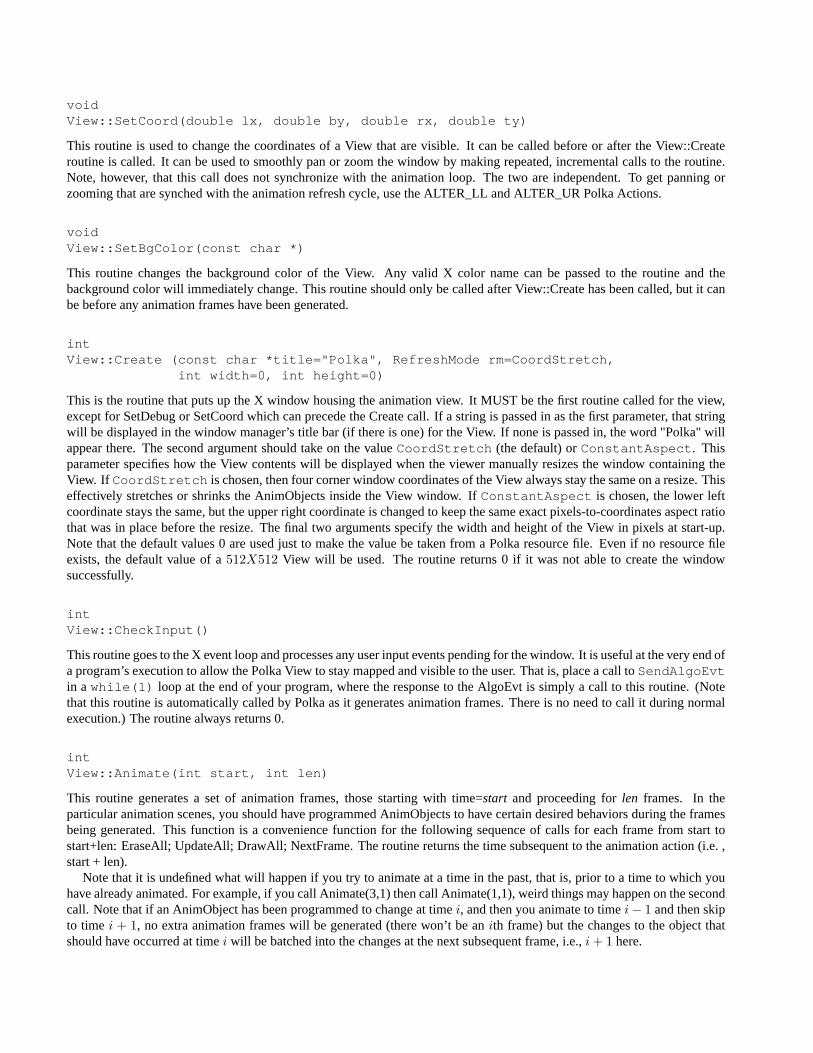
voidView::SetCoord(double lx, double by, double rx, double ty)
This routine is used to change the coordinates of a View that are visible. It can be called before or after the View::Createroutine is called. It can be used to smoothly pan or zoom the window by making repeated, incremental calls to the routine.Note, however, that this call does not synchronize with the animation loop. The two are independent. To get panning orzooming that are synched with the animation refresh cycle, use the ALTER_LL and ALTER_UR Polka Actions.
voidView::SetBgColor(const char *)
This routine changes the background color of the View. Any valid X color name can be passed to the routine and thebackground color will immediately change. This routine should only be called after View::Create has been called, but it canbe before any animation frames have been generated.
intView::Create (const char *title="Polka", RefreshMode rm=CoordStretch,
int width=0, int height=0)
This is the routine that puts up the X window housing the animation view. It MUST be the first routine called for the view,except for SetDebug or SetCoord which can precede the Create call. If a string is passed in as the first parameter, that stringwill be displayed in the window manager’s title bar (if there is one) for the View. If none is passed in, the word "Polka" willappear there. The second argument should take on the valueCoordStretch (the default) orConstantAspect. Thisparameter specifies how the View contents will be displayed when the viewer manually resizes the window containing theView. If CoordStretch is chosen, then four corner window coordinates of the View always stay the same on a resize. Thiseffectively stretches or shrinks the AnimObjects inside the View window. IfConstantAspect is chosen, the lower leftcoordinate stays the same, but the upper right coordinate is changed to keep the same exact pixels-to-coordinates aspect ratiothat was in place before the resize. The final two arguments specify the width and height of the View in pixels at start-up.Note that the default values 0 are used just to make the value be taken from a Polka resource file. Even if no resource fileexists, the default value of a512X512 View will be used. The routine returns 0 if it was not able to create the windowsuccessfully.
intView::CheckInput()
This routine goes to the X event loop and processes any user input events pending for the window. It is useful at the very end ofa program’s execution to allow the Polka View to stay mapped and visible to the user. That is, place a call toSendAlgoEvtin awhile(1) loop at the end of your program, where the response to the AlgoEvt is simply a call to this routine. (Notethat this routine is automatically called by Polka as it generates animation frames. There is no need to call it during normalexecution.) The routine always returns 0.
intView::Animate(int start, int len)
This routine generates a set of animation frames, those starting with time=start and proceeding forlen frames. In theparticular animation scenes, you should have programmed AnimObjects to have certain desired behaviors during the framesbeing generated. This function is a convenience function for the following sequence of calls for each frame from start tostart+len: EraseAll; UpdateAll; DrawAll; NextFrame. The routine returns the time subsequent to the animation action (i.e. ,start + len).
Note that it is undefined what will happen if you try to animate at a time in the past, that is, prior to a time to which youhave already animated. For example, if you call Animate(3,1) then call Animate(1,1), weird things may happen on the secondcall. Note that if an AnimObject has been programmed to change at timei, and then you animate to timei − 1 and then skipto time i + 1, no extra animation frames will be generated (there won’t be anith frame) but the changes to the object thatshould have occurred at timei will be batched into the changes at the next subsequent frame, i.e.,i + 1 here.
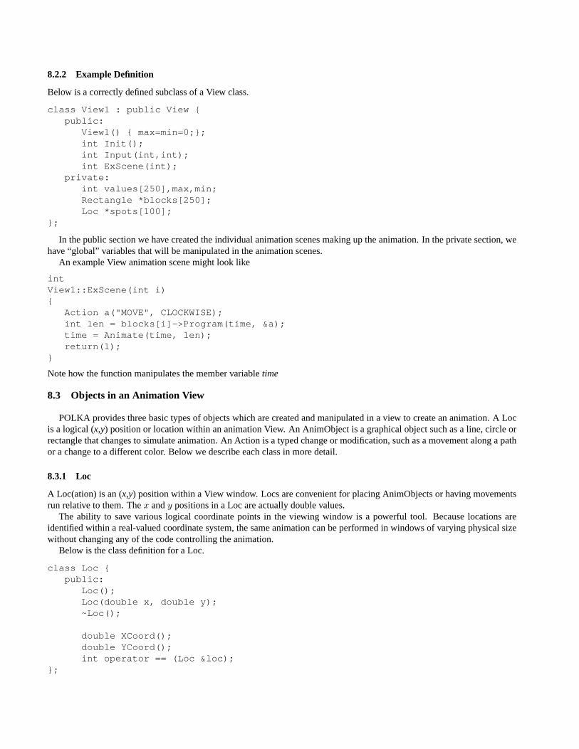
8.2.2 Example Definition
Below is a correctly defined subclass of a View class.
class View1 : public View {public:
View1() { max=min=0;};int Init();int Input(int,int);int ExScene(int);
private:int values[250],max,min;Rectangle *blocks[250];Loc *spots[100];
};
In the public section we have created the individual animation scenes making up the animation. In the private section, wehave “global” variables that will be manipulated in the animation scenes.
An example View animation scene might look like
intView1::ExScene(int i){
Action a("MOVE", CLOCKWISE);int len = blocks[i]->Program(time, &a);time = Animate(time, len);return(1);
}
Note how the function manipulates the member variabletime
8.3 Objects in an Animation View
POLKA provides three basic types of objects which are created and manipulated in a view to create an animation. A Locis a logical (x,y) position or location within an animation View. An AnimObject is a graphical object such as a line, circle orrectangle that changes to simulate animation. An Action is a typed change or modification, such as a movement along a pathor a change to a different color. Below we describe each class in more detail.
8.3.1 Loc
A Loc(ation) is an (x,y) position within a View window. Locs are convenient for placing AnimObjects or having movementsrun relative to them. Thex andy positions in a Loc are actually double values.
The ability to save various logical coordinate points in the viewing window is a powerful tool. Because locations areidentified within a real-valued coordinate system, the same animation can be performed in windows of varying physical sizewithout changing any of the code controlling the animation.
Below is the class definition for a Loc.
class Loc {public:
Loc();Loc(double x, double y);~Loc();
double XCoord();double YCoord();int operator == (Loc &loc);
};
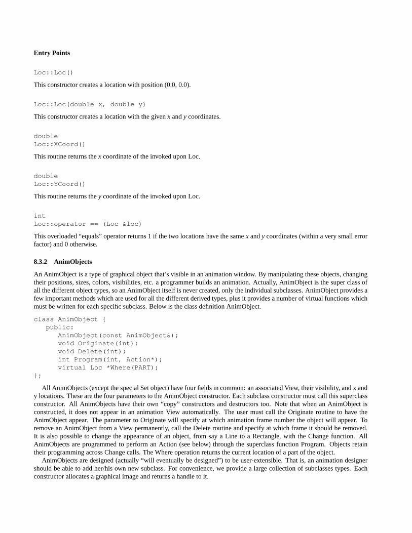
Entry Points
Loc::Loc()
This constructor creates a location with position (0.0, 0.0).
Loc::Loc(double x, double y)
This constructor creates a location with the givenx andy coordinates.
doubleLoc::XCoord()
This routine returns thex coordinate of the invoked upon Loc.
doubleLoc::YCoord()
This routine returns they coordinate of the invoked upon Loc.
intLoc::operator == (Loc &loc)
This overloaded “equals” operator returns 1 if the two locations have the samex andy coordinates (within a very small errorfactor) and 0 otherwise.
8.3.2 AnimObjects
An AnimObject is a type of graphical object that’s visible in an animation window. By manipulating these objects, changingtheir positions, sizes, colors, visibilities, etc. a programmer builds an animation. Actually, AnimObject is the super class ofall the different object types, so an AnimObject itself is never created, only the individual subclasses. AnimObject provides afew important methods which are used for all the different derived types, plus it provides a number of virtual functions whichmust be written for each specific subclass. Below is the class definition AnimObject.
class AnimObject {public:
AnimObject(const AnimObject&);void Originate(int);void Delete(int);int Program(int, Action*);virtual Loc *Where(PART);
};
All AnimObjects (except the special Set object) have four fields in common: an associated View, their visibility, and x andy locations. These are the four parameters to the AnimObject constructor. Each subclass constructor must call this superclassconstructor. All AnimObjects have their own “copy” constructors and destructors too. Note that when an AnimObject isconstructed, it does not appear in an animation View automatically. The user must call the Originate routine to have theAnimObject appear. The parameter to Originate will specify at which animation frame number the object will appear. Toremove an AnimObject from a View permanently, call the Delete routine and specify at which frame it should be removed.It is also possible to change the appearance of an object, from say a Line to a Rectangle, with the Change function. AllAnimObjects are programmed to perform an Action (see below) through the superclass function Program. Objects retaintheir programming across Change calls. The Where operation returns the current location of a part of the object.
AnimObjects are designed (actually “will eventually be designed”) to be user-extensible. That is, an animation designershould be able to add her/his own new subclass. For convenience, we provide a large collection of subclasses types. Eachconstructor allocates a graphical image and returns a handle to it.
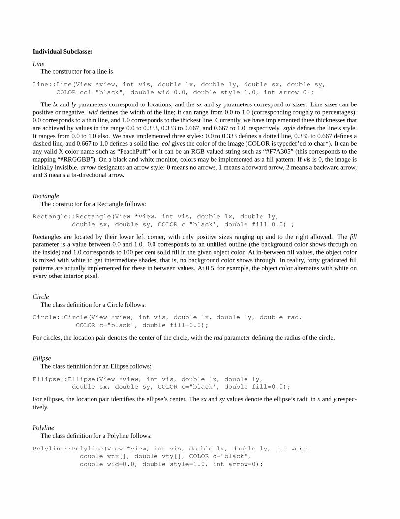
Individual Subclasses
LineThe constructor for a line is
Line::Line(View *view, int vis, double lx, double ly, double sx, double sy,COLOR col="black", double wid=0.0, double style=1.0, int arrow=0);
The lx and ly parameters correspond to locations, and thesx andsy parameters correspond to sizes. Line sizes can bepositive or negative.wid defines the width of the line; it can range from 0.0 to 1.0 (corresponding roughly to percentages).0.0 corresponds to a thin line, and 1.0 corresponds to the thickest line. Currently, we have implemented three thicknesses thatare achieved by values in the range 0.0 to 0.333, 0.333 to 0.667, and 0.667 to 1.0, respectively.style defines the line’s style.It ranges from 0.0 to 1.0 also. We have implemented three styles: 0.0 to 0.333 defines a dotted line, 0.333 to 0.667 defines adashed line, and 0.667 to 1.0 defines a solid line.col gives the color of the image (COLOR is typedef’ed to char*). It can beany valid X color name such as “PeachPuff” or it can be an RGB valued string such as “#F7A305” (this corresponds to themapping “#RRGGBB”). On a black and white monitor, colors may be implemented as a fill pattern. Ifvis is 0, the image isinitially invisible. arrow designates an arrow style: 0 means no arrows, 1 means a forward arrow, 2 means a backward arrow,and 3 means a bi-directional arrow.
RectangleThe constructor for a Rectangle follows:
Rectangle::Rectangle(View *view, int vis, double lx, double ly,double sx, double sy, COLOR c="black", double fill=0.0) ;
Rectangles are located by their lower left corner, with only positive sizes ranging up and to the right allowed. Thefillparameter is a value between 0.0 and 1.0. 0.0 corresponds to an unfilled outline (the background color shows through onthe inside) and 1.0 corresponds to 100 per cent solid fill in the given object color. At in-between fill values, the object coloris mixed with white to get intermediate shades, that is, no background color shows through. In reality, forty graduated fillpatterns are actually implemented for these in between values. At 0.5, for example, the object color alternates with white onevery other interior pixel.
CircleThe class definition for a Circle follows:
Circle::Circle(View *view, int vis, double lx, double ly, double rad,COLOR c="black", double fill=0.0);
For circles, the location pair denotes the center of the circle, with therad parameter defining the radius of the circle.
EllipseThe class definition for an Ellipse follows:
Ellipse::Ellipse(View *view, int vis, double lx, double ly,double sx, double sy, COLOR c="black", double fill=0.0);
For ellipses, the location pair identifies the ellipse’s center. Thesx andsy values denote the ellipse’s radii inx andy respec-tively.
PolylineThe class definition for a Polyline follows:
Polyline::Polyline(View *view, int vis, double lx, double ly, int vert,double vtx[], double vty[], COLOR c="black",double wid=0.0, double style=1.0, int arrow=0);
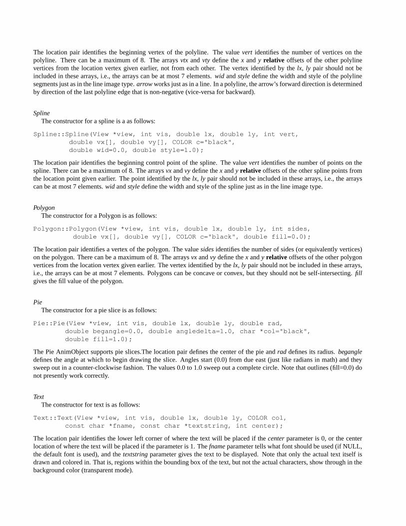
The location pair identifies the beginning vertex of the polyline. The valuevert identifies the number of vertices on thepolyline. There can be a maximum of 8. The arraysvtx andvty define thex andy relative offsets of the other polylinevertices from the location vertex given earlier, not from each other. The vertex identified by thelx, ly pair should not beincluded in these arrays, i.e., the arrays can be at most 7 elements.wid andstyle define the width and style of the polylinesegments just as in the line image type.arrow works just as in a line. In a polyline, the arrow’s forward direction is determinedby direction of the last polyline edge that is non-negative (vice-versa for backward).
SplineThe constructor for a spline is a as follows:
Spline::Spline(View *view, int vis, double lx, double ly, int vert,double vx[], double vy[], COLOR c="black",double wid=0.0, double style=1.0);
The location pair identifies the beginning control point of the spline. The valuevert identifies the number of points on thespline. There can be a maximum of 8. The arraysvx andvy define thex andy relative offsets of the other spline points fromthe location point given earlier. The point identified by thelx, ly pair should not be included in these arrays, i.e., the arrayscan be at most 7 elements.wid andstyle define the width and style of the spline just as in the line image type.
PolygonThe constructor for a Polygon is as follows:
Polygon::Polygon(View *view, int vis, double lx, double ly, int sides,double vx[], double vy[], COLOR c="black", double fill=0.0);
The location pair identifies a vertex of the polygon. The valuesides identifies the number of sides (or equivalently vertices)on the polygon. There can be a maximum of 8. The arraysvx andvy define thex andy relative offsets of the other polygonvertices from the location vertex given earlier. The vertex identified by thelx, ly pair should not be included in these arrays,i.e., the arrays can be at most 7 elements. Polygons can be concave or convex, but they should not be self-intersecting.fillgives the fill value of the polygon.
PieThe constructor for a pie slice is as follows:
Pie::Pie(View *view, int vis, double lx, double ly, double rad,double begangle=0.0, double angledelta=1.0, char *col="black",double fill=1.0);
The Pie AnimObject supports pie slices.The location pair defines the center of the pie andrad defines its radius.begangledefines the angle at which to begin drawing the slice. Angles start (0.0) from due east (just like radians in math) and theysweep out in a counter-clockwise fashion. The values 0.0 to 1.0 sweep out a complete circle. Note that outlines (fill=0.0) donot presently work correctly.
TextThe constructor for text is as follows:
Text::Text(View *view, int vis, double lx, double ly, COLOR col,const char *fname, const char *textstring, int center);
The location pair identifies the lower left corner of where the text will be placed if thecenter parameter is 0, or the centerlocation of where the text will be placed if the parameter is 1. Thefname parameter tells what font should be used (if NULL,the default font is used), and thetextstring parameter gives the text to be displayed. Note that only the actual text itself isdrawn and colored in. That is, regions within the bounding box of the text, but not the actual characters, show through in thebackground color (transparent mode).
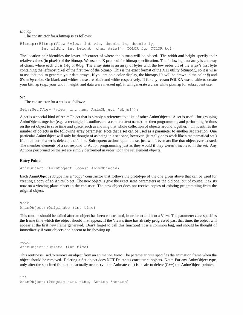
BitmapThe constructor for a bitmap is as follows:
Bitmap::Bitmap(View *view, int vis, double lx, double ly,int width, int height, char data[], COLOR fg, COLOR bg);
The location pair identifies the lower left corner of where the bitmap will be placed. The width and height specify theirrelative values (in pixels) of the bitmap. We use the X protocol for bitmap specification. The following data array is an arrayof chars, where each bit is 1-fg or 0-bg. The arraydata is an array of bytes with the low order bit of the array’s first bytecontaining the leftmost pixel of the first row of the bitmap. This is the exact format of the X11 utilitybitmap(1), so it is wiseto use that tool to generate your data arrays. If you are on a color display, the bitmaps 1’s will be drawn in the colorfg and0’s in bg color. On black-and-whites these are black and white respectively. If for any reason POLKA was unable to createyour bitmap (e.g., your width, height, and data were messed up), it will generate a clear white pixmap for subsequent use.
SetThe constructor for a set is as follows:
Set::Set(View *view, int num, AnimObject *objs[]);
A set is a special kind of AnimObject that is simply a reference to a list of other AnimObjects. A set is useful for groupingAnimObjects together (e.g. , a rectangle, its outline, and a centered text name) and then programming and performing Actionson the set object to save time and space, such as moving that whole collection of objects around together.num identifies thenumber of objects in the following array parameter. Note that a set can be used as a parameter to another set creation. Oneparticular AnimObject will only be thought of as being in a set once, however. (It really does work like a mathematical set.)If a member of a set is deleted, that’s fine. Subsequent actions upon the set just won’t even act like that object ever existed.The member elements of a set respond to Action programming just as they would if they weren’t involved in the set. AnyActions performed on the set are simply performed in order upon the set element objects.
Entry Points
AnimObject::AnimObject (const AnimObject&)
Each AnimObject subtype has a “copy” constructor that follows the prototype of the one given above that can be used forcreating a copy of an AnimObject. The new object is give the exact same parameters as the old one, but of course, it existsnow on a viewing plane closer to the end-user. The new object does not receive copies of existing programming from theoriginal object.
voidAnimObject::Originate (int time)
This routine should be called after an object has been constructed, in order to add it to a View. The parametertime specifiesthe frame time which the object should first appear. If the View’s time has already progressed past that time, the object willappear at the first new frame generated. Don’t forget to call this function! It is a common bug, and should be thought ofimmediately if your objects don’t seem to be showing up.
voidAnimObject::Delete (int time)
This routine is used to remove an object from an animation View. The parametertime specifies the animation frame when theobject should be removed. Deleting a Set object does NOT Delete its constituent objects. Note: For any AnimObject type,only after the specified frame time actually occurs (via the Animate call) is it safe to delete (C++) the AnimObject pointer.
intAnimObject::Program (int time, Action *action)
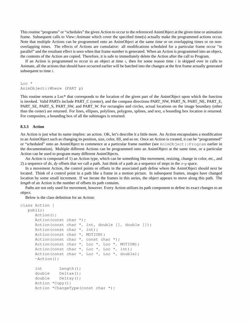
This routine “programs” or “schedules” the given Action to occur to the referenced AnimObject at the given time or animationframe. Subsequent calls to View::Animate which cover the specified time(s) actually make the programmed actions occur.Note that multiple Actions can be programmed onto an AnimObject at the same time or on overlapping times or on non-overlapping times. The effects of Actions are cumulative: all modifications scheduled for a particular frame occur “inparallel” and the resultant effect is seen when that frame number is generated. When an Action is programmed into an object,the contents of the Action are copied. Therefore, it is safe to immediately delete the Action after the call to Program.
If an Action is programmed to occur to an object at timei, then for some reason timei is skipped over in calls toAnimate, all the actions that should have occurred earlier will be batched into the changes at the first frame actually generatedsubsequent to timei.
Loc *AnimObject::Where (PART p)
This routine returns a Loc* that corresponds to the location of the given part of the AnimObject upon which the functionis invoked. Valid PARTs include PART_C (center), and the compass directions PART_NW, PART_N, PART_NE, PART_E,PART_SE, PART_S, PART_SW, and PART_W. For rectangles and circles, actual locations on the image boundary (otherthan the center) are returned. For lines, ellipses, polylines, polygons, splines, and text, a bounding box location is returned.For composites, a bounding box of all the subimages is returned.
8.3.3 Action
An Action is just what its name implies: an action. OK, let’s describe it a little more. An Action encapsulates a modificationto an AnimObject such as changing its position, size, color, fill, and so on. Once an Action is created, it can be “programmed”or “scheduled” onto an AnimObject to commence at a particular frame number (seeAnimObject::Program earlier inthe documentation). Multiple different Actions can be programmed onto an AnimObject at the same time, or a particularAction can be used to program many different AnimObjects.
An Action is composed of 1) an Action type, which can be something like movement, resizing, change in color, etc., and2) a sequence ofdx, dy offsets that we call a path. Just think of a path as a sequence of steps in thex-y space.
In a movement Action, the control points or offsets in the associated path define where the AnimObject should next belocated. Think of a control point in a path like a frame in a motion picture. In subsequent frames, images have changedlocation by some small increment. If we iterate the frames in this series, the object appears to move along this path. Thelength of an Action is the number of offsets its path contains.
Paths are not only used for movement, however. Every Action utilizes its path component to define its exact changes to anobject.
Below is the class definition for an Action:
class Action {public:
Action();Action(const char *);Action(const char *, int, double [], double []);Action(const char *, int);Action(const char *, MOTION);Action(const char *, const char *);Action(const char *, Loc *, Loc *, MOTION);Action(const char *, Loc *, Loc *, int);Action(const char *, Loc *, Loc *, double);~Action();
int Length();double Deltax();double Deltay();Action *Copy();Action *ChangeType(const char *);
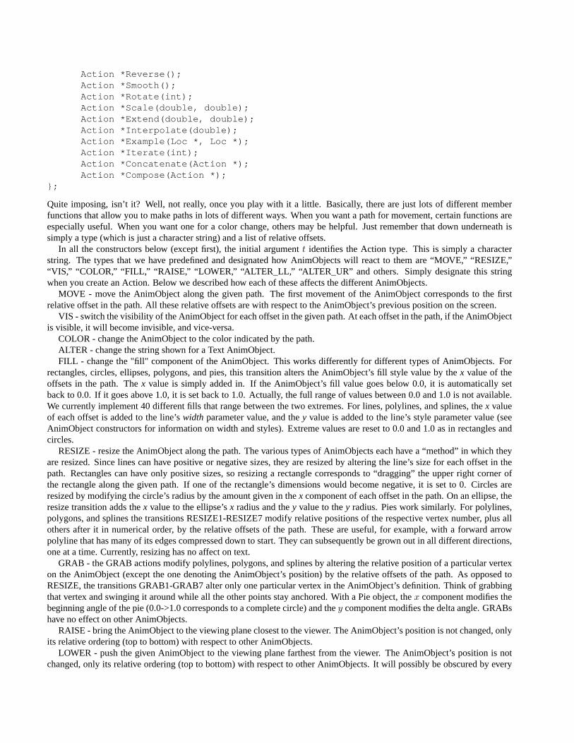
Action *Reverse();Action *Smooth();Action *Rotate(int);Action *Scale(double, double);Action *Extend(double, double);Action *Interpolate(double);Action *Example(Loc *, Loc *);Action *Iterate(int);Action *Concatenate(Action *);Action *Compose(Action *);
};
Quite imposing, isn’t it? Well, not really, once you play with it a little. Basically, there are just lots of different memberfunctions that allow you to make paths in lots of different ways. When you want a path for movement, certain functions areespecially useful. When you want one for a color change, others may be helpful. Just remember that down underneath issimply a type (which is just a character string) and a list of relative offsets.
In all the constructors below (except first), the initial argumentt identifies the Action type. This is simply a characterstring. The types that we have predefined and designated how AnimObjects will react to them are “MOVE,” “RESIZE,”“VIS,” “COLOR,” “FILL,” “RAISE,” “LOWER,” “ALTER_LL,” “ALTER_UR” and others. Simply designate this stringwhen you create an Action. Below we described how each of these affects the different AnimObjects.
MOVE - move the AnimObject along the given path. The first movement of the AnimObject corresponds to the firstrelative offset in the path. All these relative offsets are with respect to the AnimObject’s previous position on the screen.
VIS - switch the visibility of the AnimObject for each offset in the given path. At each offset in the path, if the AnimObjectis visible, it will become invisible, and vice-versa.
COLOR - change the AnimObject to the color indicated by the path.ALTER - change the string shown for a Text AnimObject.FILL - change the "fill" component of the AnimObject. This works differently for different types of AnimObjects. For
rectangles, circles, ellipses, polygons, and pies, this transition alters the AnimObject’s fill style value by thex value of theoffsets in the path. Thex value is simply added in. If the AnimObject’s fill value goes below 0.0, it is automatically setback to 0.0. If it goes above 1.0, it is set back to 1.0. Actually, the full range of values between 0.0 and 1.0 is not available.We currently implement 40 different fills that range between the two extremes. For lines, polylines, and splines, thex valueof each offset is added to the line’swidth parameter value, and they value is added to the line’s style parameter value (seeAnimObject constructors for information on width and styles). Extreme values are reset to 0.0 and 1.0 as in rectangles andcircles.
RESIZE - resize the AnimObject along the path. The various types of AnimObjects each have a “method” in which theyare resized. Since lines can have positive or negative sizes, they are resized by altering the line’s size for each offset in thepath. Rectangles can have only positive sizes, so resizing a rectangle corresponds to “dragging” the upper right corner ofthe rectangle along the given path. If one of the rectangle’s dimensions would become negative, it is set to 0. Circles areresized by modifying the circle’s radius by the amount given in thex component of each offset in the path. On an ellipse, theresize transition adds thex value to the ellipse’sx radius and they value to they radius. Pies work similarly. For polylines,polygons, and splines the transitions RESIZE1-RESIZE7 modify relative positions of the respective vertex number, plus allothers after it in numerical order, by the relative offsets of the path. These are useful, for example, with a forward arrowpolyline that has many of its edges compressed down to start. They can subsequently be grown out in all different directions,one at a time. Currently, resizing has no affect on text.
GRAB - the GRAB actions modify polylines, polygons, and splines by altering the relative position of a particular vertexon the AnimObject (except the one denoting the AnimObject’s position) by the relative offsets of the path. As opposed toRESIZE, the transitions GRAB1-GRAB7 alter only one particular vertex in the AnimObject’s definition. Think of grabbingthat vertex and swinging it around while all the other points stay anchored. With a Pie object, thex component modifies thebeginning angle of the pie (0.0->1.0 corresponds to a complete circle) and they component modifies the delta angle. GRABshave no effect on other AnimObjects.
RAISE - bring the AnimObject to the viewing plane closest to the viewer. The AnimObject’s position is not changed, onlyits relative ordering (top to bottom) with respect to other AnimObjects.
LOWER - push the given AnimObject to the viewing plane farthest from the viewer. The AnimObject’s position is notchanged, only its relative ordering (top to bottom) with respect to other AnimObjects. It will possibly be obscured by every
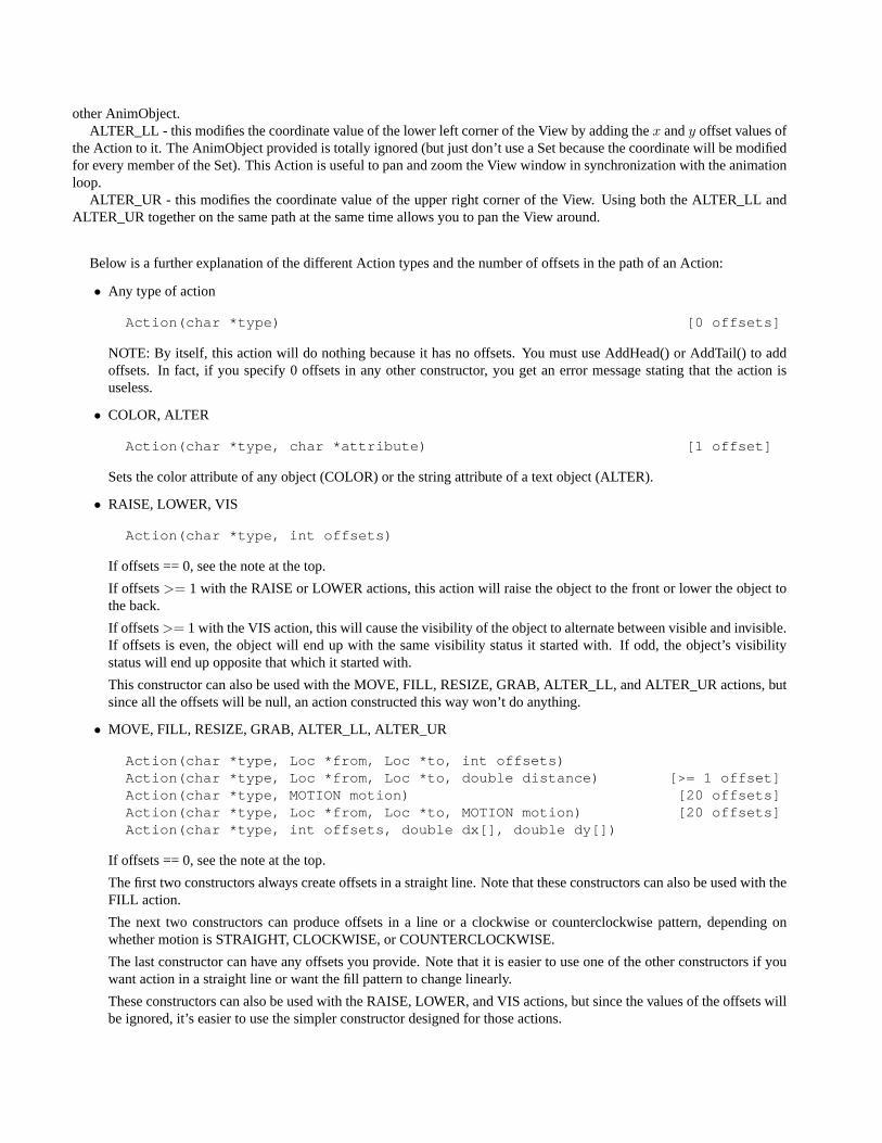
other AnimObject.ALTER_LL - this modifies the coordinate value of the lower left corner of the View by adding thex andy offset values of
the Action to it. The AnimObject provided is totally ignored (but just don’t use a Set because the coordinate will be modifiedfor every member of the Set). This Action is useful to pan and zoom the View window in synchronization with the animationloop.
ALTER_UR - this modifies the coordinate value of the upper right corner of the View. Using both the ALTER_LL andALTER_UR together on the same path at the same time allows you to pan the View around.
Below is a further explanation of the different Action types and the number of offsets in the path of an Action:
• Any type of action
Action(char *type) [0 offsets]
NOTE: By itself, this action will do nothing because it has no offsets. You must use AddHead() or AddTail() to addoffsets. In fact, if you specify 0 offsets in any other constructor, you get an error message stating that the action isuseless.
• COLOR, ALTER
Action(char *type, char *attribute) [1 offset]
Sets the color attribute of any object (COLOR) or the string attribute of a text object (ALTER).
• RAISE, LOWER, VIS
Action(char *type, int offsets)
If offsets == 0, see the note at the top.
If offsets>= 1 with the RAISE or LOWER actions, this action will raise the object to the front or lower the object tothe back.
If offsets>= 1 with the VIS action, this will cause the visibility of the object to alternate between visible and invisible.If offsets is even, the object will end up with the same visibility status it started with. If odd, the object’s visibilitystatus will end up opposite that which it started with.
This constructor can also be used with the MOVE, FILL, RESIZE, GRAB, ALTER_LL, and ALTER_UR actions, butsince all the offsets will be null, an action constructed this way won’t do anything.
• MOVE, FILL, RESIZE, GRAB, ALTER_LL, ALTER_UR
Action(char *type, Loc *from, Loc *to, int offsets)Action(char *type, Loc *from, Loc *to, double distance) [>= 1 offset]Action(char *type, MOTION motion) [20 offsets]Action(char *type, Loc *from, Loc *to, MOTION motion) [20 offsets]Action(char *type, int offsets, double dx[], double dy[])
If offsets == 0, see the note at the top.
The first two constructors always create offsets in a straight line. Note that these constructors can also be used with theFILL action.
The next two constructors can produce offsets in a line or a clockwise or counterclockwise pattern, depending onwhether motion is STRAIGHT, CLOCKWISE, or COUNTERCLOCKWISE.
The last constructor can have any offsets you provide. Note that it is easier to use one of the other constructors if youwant action in a straight line or want the fill pattern to change linearly.
These constructors can also be used with the RAISE, LOWER, and VIS actions, but since the values of the offsets willbe ignored, it’s easier to use the simpler constructor designed for those actions.
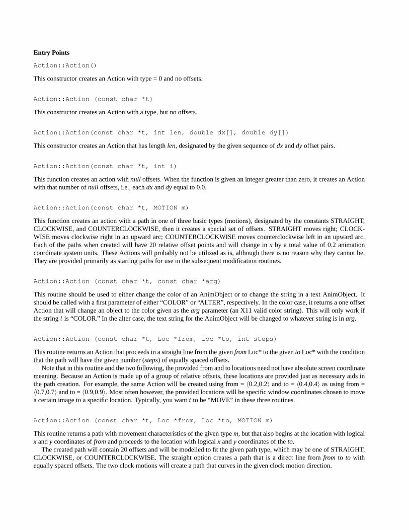
Entry Points
Action::Action()
This constructor creates an Action with type = 0 and no offsets.
Action::Action (const char *t)
This constructor creates an Action with a type, but no offsets.
Action::Action(const char *t, int len, double dx[], double dy[])
This constructor creates an Action that has lengthlen, designated by the given sequence ofdx anddy offset pairs.
Action::Action(const char *t, int i)
This function creates an action withnull offsets. When the function is given an integer greater than zero, it creates an Actionwith that number ofnull offsets, i.e., eachdx anddy equal to 0.0.
Action::Action(const char *t, MOTION m)
This function creates an action with a path in one of three basic types (motions), designated by the constants STRAIGHT,CLOCKWISE, and COUNTERCLOCKWISE, then it creates a special set of offsets. STRAIGHT moves right; CLOCK-WISE moves clockwise right in an upward arc; COUNTERCLOCKWISE moves counterclockwise left in an upward arc.Each of the paths when created will have 20 relative offset points and will change inx by a total value of 0.2 animationcoordinate system units. These Actions will probably not be utilized as is, although there is no reason why they cannot be.They are provided primarily as starting paths for use in the subsequent modification routines.
Action::Action (const char *t, const char *arg)
This routine should be used to either change the color of an AnimObject or to change the string in a text AnimObject. Itshould be called with a first parameter of either “COLOR” or “ALTER”, respectively. In the color case, it returns a one offsetAction that will change an object to the color given as thearg parameter (an X11 valid color string). This will only work ifthe stringt is “COLOR.” In the alter case, the text string for the AnimObject will be changed to whatever string is inarg.
Action::Action (const char *t, Loc *from, Loc *to, int steps)
This routine returns an Action that proceeds in a straight line from the givenfrom Loc* to the givento Loc* with the conditionthat the path will have the given number (steps) of equally spaced offsets.
Note that in this routine and the two following, the provided from and to locations need not have absolute screen coordinatemeaning. Because an Action is made up of a group of relative offsets, these locations are provided just as necessary aids inthe path creation. For example, the same Action will be created using from =〈0.2,0.2〉 and to =〈0.4,0.4〉 as using from =〈0.7,0.7〉 and to =〈0.9,0.9〉. Most often however, the provided locations will be specific window coordinates chosen to movea certain image to a specific location. Typically, you wantt to be “MOVE” in these three routines.
Action::Action (const char *t, Loc *from, Loc *to, MOTION m)
This routine returns a path with movement characteristics of the given typem, but that also begins at the location with logicalx andy coordinates offrom and proceeds to the location with logicalx andy coordinates of theto.
The created path will contain 20 offsets and will be modelled to fit the given path type, which may be one of STRAIGHT,CLOCKWISE, or COUNTERCLOCKWISE. The straight option creates a path that is a direct line fromfrom to to withequally spaced offsets. The two clock motions will create a path that curves in the given clock motion direction.
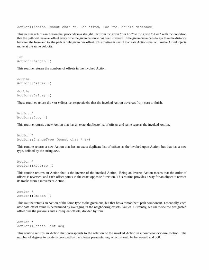
Action::Action (const char *t, Loc *from, Loc *to, double distance)
This routine returns an Action that proceeds in a straight line from the givenfrom Loc* to the givento Loc* with the conditionthat the path will have an offset every time the givendistance has been covered. If the given distance is larger than the distancebetween the from and to, the path is only given one offset. This routine is useful to create Actions that will make AnimObjectsmove at the same velocity.
intAction::Length ()
This routine returns the numbers of offsets in the invoked Action.
doubleAction::Deltax ()
doubleAction::Deltay ()
These routines return thex or y distance, respectively, that the invoked Action traverses from start to finish.
Action *Action::Copy ()
This routine returns a new Action that has an exact duplicate list of offsets and same type as the invoked Action.
Action *Action::ChangeType (const char *new)
This routine returns a new Action that has an exact duplicate list of offsets as the invoked upon Action, but that has a newtype, defined by the stringnew.
Action *Action::Reverse ()
This routine returns an Action that is the inverse of the invoked Action. Being an inverse Action means that the order ofoffsets is reversed, and each offset points in the exact opposite direction. This routine provides a way for an object to retraceits tracks from a movement Action.
Action *Action::Smooth ()
This routine returns an Action of the same type as the given one, but that has a “smoother” path component. Essentially, eachnew path offset value is determined by averaging in the neighboring offsets’ values. Currently, we use twice the designatedoffset plus the previous and subsequent offsets, divided by four.
Action *Action::Rotate (int deg)
This routine returns an Action that corresponds to the rotation of the invoked Action in a counter-clockwise motion. Thenumber of degrees to rotate is provided by the integer parameterdeg which should be between 0 and 360.
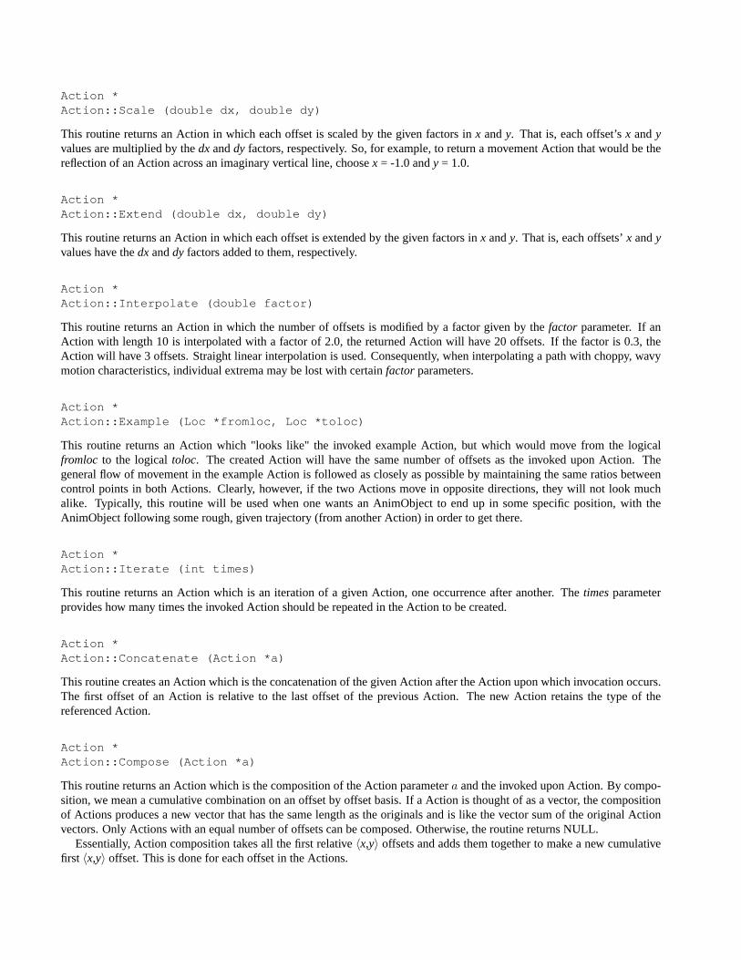
Action *Action::Scale (double dx, double dy)
This routine returns an Action in which each offset is scaled by the given factors inx andy. That is, each offset’sx andyvalues are multiplied by thedx anddy factors, respectively. So, for example, to return a movement Action that would be thereflection of an Action across an imaginary vertical line, choosex = -1.0 andy = 1.0.
Action *Action::Extend (double dx, double dy)
This routine returns an Action in which each offset is extended by the given factors inx andy. That is, each offsets’x andyvalues have thedx anddy factors added to them, respectively.
Action *Action::Interpolate (double factor)
This routine returns an Action in which the number of offsets is modified by a factor given by thefactor parameter. If anAction with length 10 is interpolated with a factor of 2.0, the returned Action will have 20 offsets. If the factor is 0.3, theAction will have 3 offsets. Straight linear interpolation is used. Consequently, when interpolating a path with choppy, wavymotion characteristics, individual extrema may be lost with certainfactor parameters.
Action *Action::Example (Loc *fromloc, Loc *toloc)
This routine returns an Action which "looks like" the invoked example Action, but which would move from the logicalfromloc to the logicaltoloc. The created Action will have the same number of offsets as the invoked upon Action. Thegeneral flow of movement in the example Action is followed as closely as possible by maintaining the same ratios betweencontrol points in both Actions. Clearly, however, if the two Actions move in opposite directions, they will not look muchalike. Typically, this routine will be used when one wants an AnimObject to end up in some specific position, with theAnimObject following some rough, given trajectory (from another Action) in order to get there.
Action *Action::Iterate (int times)
This routine returns an Action which is an iteration of a given Action, one occurrence after another. Thetimes parameterprovides how many times the invoked Action should be repeated in the Action to be created.
Action *Action::Concatenate (Action *a)
This routine creates an Action which is the concatenation of the given Action after the Action upon which invocation occurs.The first offset of an Action is relative to the last offset of the previous Action. The new Action retains the type of thereferenced Action.
Action *Action::Compose (Action *a)
This routine returns an Action which is the composition of the Action parametera and the invoked upon Action. By compo-sition, we mean a cumulative combination on an offset by offset basis. If a Action is thought of as a vector, the compositionof Actions produces a new vector that has the same length as the originals and is like the vector sum of the original Actionvectors. Only Actions with an equal number of offsets can be composed. Otherwise, the routine returns NULL.
Essentially, Action composition takes all the first relative〈x,y〉 offsets and adds them together to make a new cumulativefirst 〈x,y〉 offset. This is done for each offset in the Actions.
References
[1] LYDIAN, http://www.cs.chalmers.se/∼lydian
[2] John T. Stasko. POLKA Animation Designer’s Package,Lite Version, College of Computing, Georgia Institute ofTechnology, Atlanta, GA 30332-0280
[3] LEDA GraphWin,http://www.algorithmic-solutions.info/leda_guide/GraphWin.html
[4] P. Spirakis, B. Tampakas, M. Papatriantafilou, K. Konstantoulis, K. Vlaxodimitropoulos, V. Antonopoulos, P. Kazazis,T. Metallidou, S. Spartiotis. The DSS Tool – A Distributed Systems Simulator.Proceedings of the 9th Annual Sym-posium on Theoretical Aspects of Computer Science (STACS ’92), 1992, Lecture Notes in Computer Science 577,Springer-Verlag.
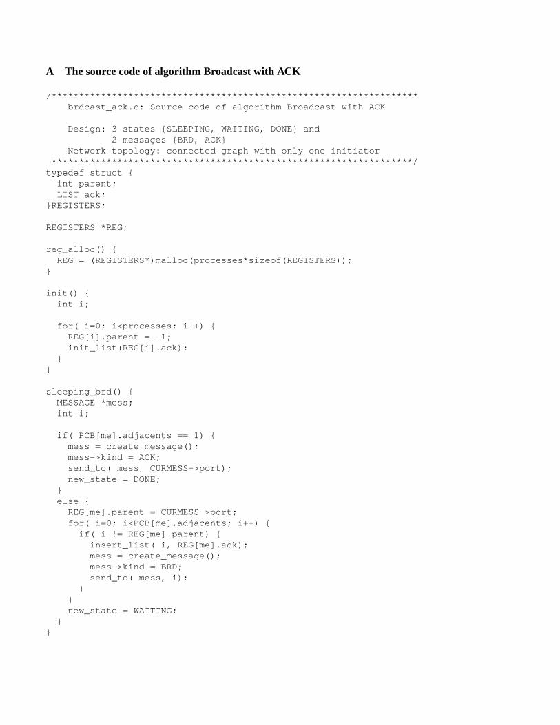
A The source code of algorithm Broadcast with ACK
/*******************************************************************brdcast_ack.c: Source code of algorithm Broadcast with ACK
Design: 3 states {SLEEPING, WAITING, DONE} and2 messages {BRD, ACK}
Network topology: connected graph with only one initiator******************************************************************/typedef struct {int parent;LIST ack;
}REGISTERS;
REGISTERS *REG;
reg_alloc() {REG = (REGISTERS*)malloc(processes*sizeof(REGISTERS));
}
init() {int i;
for( i=0; i<processes; i++) {REG[i].parent = -1;init_list(REG[i].ack);
}}
sleeping_brd() {MESSAGE *mess;int i;
if( PCB[me].adjacents == 1) {mess = create_message();mess->kind = ACK;send_to( mess, CURMESS->port);new_state = DONE;
}else {
REG[me].parent = CURMESS->port;for( i=0; i<PCB[me].adjacents; i++) {if( i != REG[me].parent) {insert_list( i, REG[me].ack);mess = create_message();mess->kind = BRD;send_to( mess, i);
}}new_state = WAITING;
}}
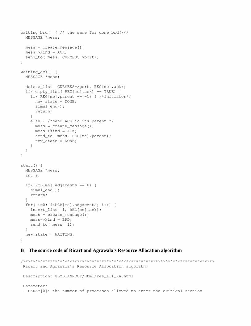
waiting_brd() { /* the same for done_brd()*/MESSAGE *mess;
mess = create_message();mess->kind = ACK;send_to( mess, CURMESS->port);
}
waiting_ack() {MESSAGE *mess;
delete_list( CURMESS->port, REG[me].ack);if( empty_list( REG[me].ack) == TRUE) {
if( REG[me].parent == -1) { /*initiator*/new_state = DONE;simul_end();return;
}else { /*send ACK to its parent */mess = create_message();mess->kind = ACK;send_to( mess, REG[me].parent);new_state = DONE;
}}
}
start() {MESSAGE *mess;int i;
if( PCB[me].adjacents == 0) {simul_end();return;
}for( i=0; i<PCB[me].adjacents; i++) {
insert_list( i, REG[me].ack);mess = create_message();mess->kind = BRD;send_to( mess, i);
}new_state = WAITING;
}
B The source code of Ricart and Agrawala’s Resource Allocation algorithm
/******************************************************************************Ricart and Agrawala’s Resource Allocation algorithm
Description: $LYDIANROOT/Html/res_all_RA.html
Parameter:- PARAM[0]: the number of processes allowed to enter the critical section
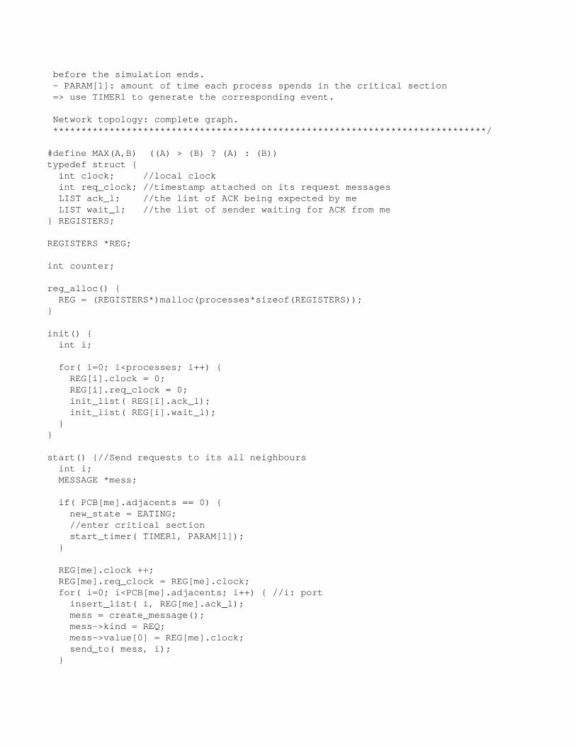
before the simulation ends.- PARAM[1]: amount of time each process spends in the critical section=> use TIMER1 to generate the corresponding event.
Network topology: complete graph.*****************************************************************************/
#define MAX(A,B) ((A) > (B) ? (A) : (B))typedef struct {int clock; //local clockint req_clock; //timestamp attached on its request messagesLIST ack_l; //the list of ACK being expected by meLIST wait_l; //the list of sender waiting for ACK from me
} REGISTERS;
REGISTERS *REG;
int counter;
reg_alloc() {REG = (REGISTERS*)malloc(processes*sizeof(REGISTERS));
}
init() {int i;
for( i=0; i<processes; i++) {REG[i].clock = 0;REG[i].req_clock = 0;init_list( REG[i].ack_l);init_list( REG[i].wait_l);
}}
start() {//Send requests to its all neighboursint i;MESSAGE *mess;
if( PCB[me].adjacents == 0) {new_state = EATING;//enter critical sectionstart_timer( TIMER1, PARAM[1]);
}
REG[me].clock ++;REG[me].req_clock = REG[me].clock;for( i=0; i<PCB[me].adjacents; i++) { //i: port
insert_list( i, REG[me].ack_l);mess = create_message();mess->kind = REQ;mess->value[0] = REG[me].clock;send_to( mess, i);
}
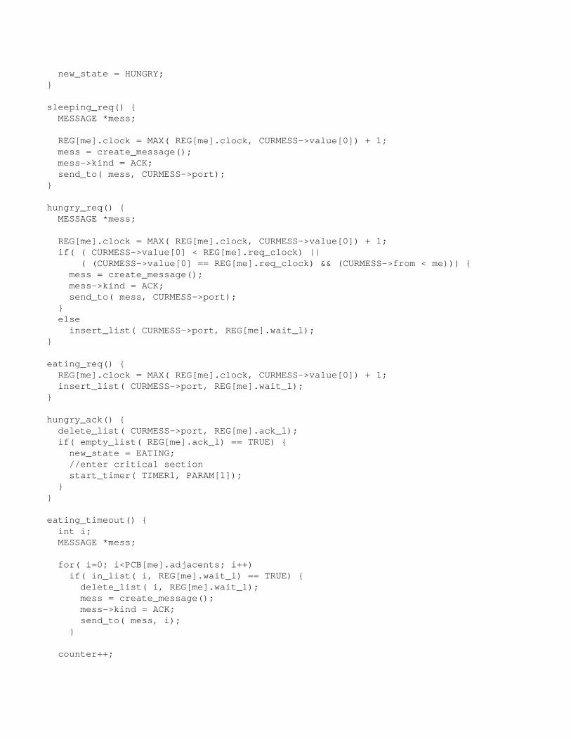
new_state = HUNGRY;}
sleeping_req() {MESSAGE *mess;
REG[me].clock = MAX( REG[me].clock, CURMESS->value[0]) + 1;mess = create_message();mess->kind = ACK;send_to( mess, CURMESS->port);
}
hungry_req() {MESSAGE *mess;
REG[me].clock = MAX( REG[me].clock, CURMESS->value[0]) + 1;if( ( CURMESS->value[0] < REG[me].req_clock) ||
( (CURMESS->value[0] == REG[me].req_clock) && (CURMESS->from < me))) {mess = create_message();mess->kind = ACK;send_to( mess, CURMESS->port);
}else
insert_list( CURMESS->port, REG[me].wait_l);}
eating_req() {REG[me].clock = MAX( REG[me].clock, CURMESS->value[0]) + 1;insert_list( CURMESS->port, REG[me].wait_l);
}
hungry_ack() {delete_list( CURMESS->port, REG[me].ack_l);if( empty_list( REG[me].ack_l) == TRUE) {
new_state = EATING;//enter critical sectionstart_timer( TIMER1, PARAM[1]);
}}
eating_timeout() {int i;MESSAGE *mess;
for( i=0; i<PCB[me].adjacents; i++)if( in_list( i, REG[me].wait_l) == TRUE) {delete_list( i, REG[me].wait_l);mess = create_message();mess->kind = ACK;send_to( mess, i);
}
counter++;
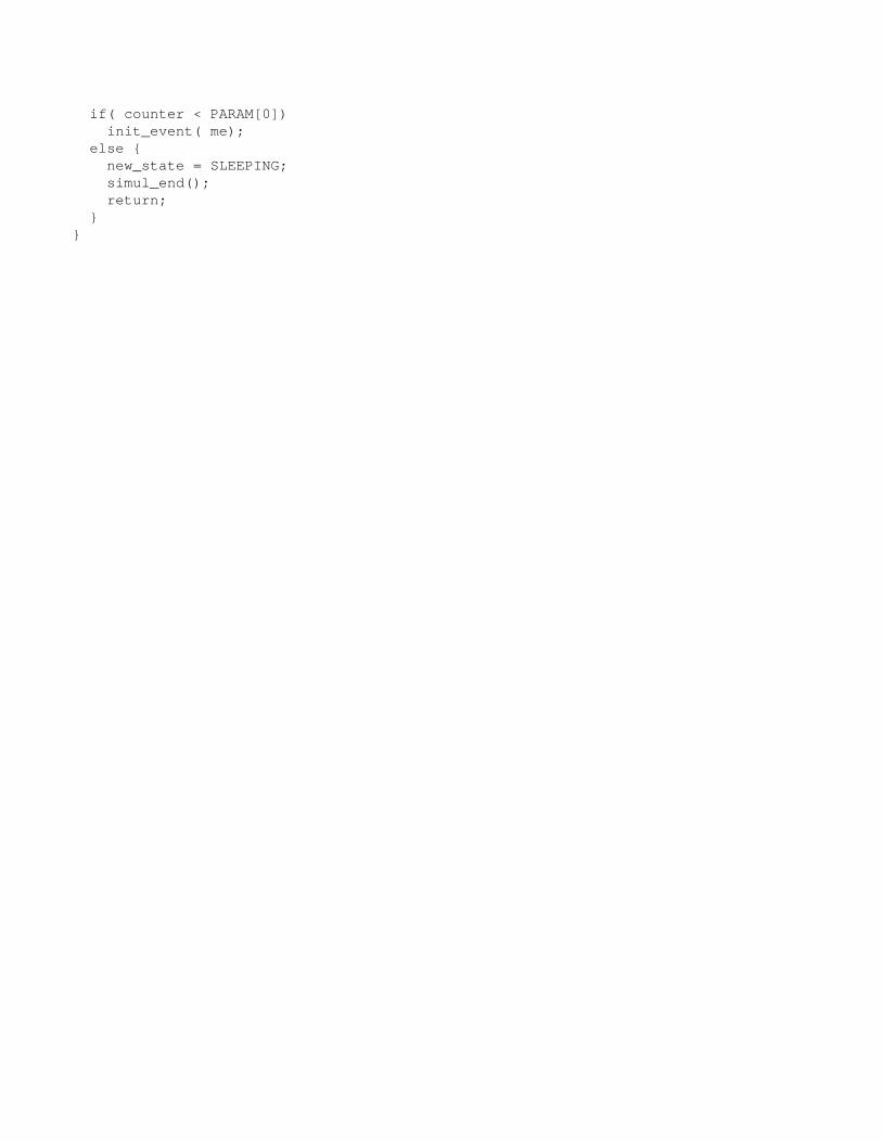
if( counter < PARAM[0])init_event( me);
else {new_state = SLEEPING;simul_end();return;
}}


