Simulation model for NOx distributions in a street canyon with air purifying pavement
H.T.J. Overman

Simulation model for NOx distributions in a street canyon with air purifying pavement Master thesis of H.T.J. Overman Master: Civil Engineering & Management Supervisors: Dr. Eng. M.M. Ballari Prof. Dr. Ir. H.J.H. Brouwers Department of Construction Management & Engineering, Faculty of Engineering Technology, University of Twente, Enschede, the Netherlands August 2009
Abstract In Hengelo (Overijssel, NL) a street (Castorweg) will be paved with air purifying pavement. The top layer of this pavement contains TiO2, which serves as a catalyst for the degradation process of the car emission gases NO and NO2, under the influence of UV light. A 2‐dimensional simulation model is made that describes the distributions of pollutant concentrations and the effect of the air purifying pavement on these concentrations throughout a cross‐section of this street canyon. The simulation model assumes a wind direction perpendicular to the street, and takes the effects of wind speed, relative humidity, UV irradiance, traffic density, background concentrations and atmospheric reactions into account. The atmospheric reactions under the influence of UV irradiance generally account for a large reduction of NO and NO2 during the day. For a relatively quiet street like the Castorweg, simulations show that the air purifying pavement can reduce the NO and O3 levels in the street at a height of 1.50m with 2% and the NO2 levels with 10%, for an average late winter day. In more favourable winter conditions the NO and NO2 reduction can reach 3 and 17% respectively. For lower heights the NOx reduction increases significantly. A higher temperature could cause an increase in the NOx levels, consequently further increasing the reduction by the air purifying pavement. For streets with higher buildings, or with a wind direction parallel to the street the residence time of NOx near the air purifying pavement would be longer, yielding a higher NOx reduction.


Preface During the final year of my Civil Engineering & Management master course, I came into contact with the subject of air purifying pavement. I had never heard of anything like it, but it immediately caught my attention. And when I was told that there was an assignment available for a master thesis project, I jumped at the chance to become a part of this research. What drew me into this project was mainly the versatility. I could put elements of my bachelor course in Applied Physics into this project as well as chemical fundamentals, which already attracted me before I came to the university. What made it even better was the fact that these fundamentals were directly applied in an innovative product. This report is the product of my master thesis project which lasted from January to August 2009. The initial assignment was to develop a simulation model of the NOx degradation by air purifying pavement in the Castorweg (Hengelo, NL). Another part of the research would be actual street measurements. During the project the research was extended in two ways. First an extra model was made to simulate the reactor used to test the air purifying stones. And secondly, it turned out that atmospheric reactions could not be neglected as was assumed before the first measurements. This led to a relatively large amount of extra research and modelling to describe the influence of these reactions, not only theoretically, but also practically in the street simulation model. Even though the days of measuring in the street were cold and long, I can honestly say that I enjoyed the project. As I already explained, I found the subject very interesting. On top of that I had some really extensive and interesting conversations with my supervisor: Milagros, thank you for the feedback, the guidance and both the on‐ and off‐topic discussions. I would also like to thank my other supervisor Prof. Dr. Ir. Brouwers for stimulating me to keep up the pace and for the sharp and useful feedback. Finally I would like to thank my parents who kept supporting me all the way, even though I took a little longer to graduate than they hoped, and most of all my girlfriend Annemarie: for believing in me, supporting me, travelling to see me every week, laughing with me, and everything else she did for me during this project. Next is a short overview of what can be found in this report: Chapter 1 presents an introduction into the subject of air purifying pavement. The problem definition for this research project will be explained in chapter 2. The results from the street measurements are presented in chapter 3, after which the software and fundamental elements required for the simulation model are discussed in chapter 4. In chapter 5 a simulation model for the reactor that is used in the laboratory experiments is presented. The fundamental elements of the simulation model for the street are discussed in chapter 6, after which the results of this model are discussed in chapter 7. Finally in chapter 8 the conclusions for this project are presented along with several recommendations for future research.
Contents 1 Introduction ............................................................................................................................ 1 2 Problem definition .................................................................................................................. 3 2.1 Research problem ................................................................................................................... 3 2.2 Objectives ................................................................................................................................ 3 2.3 Research questions ................................................................................................................. 3 2.4 Scope ....................................................................................................................................... 4 2.5 Research results ...................................................................................................................... 4
3 Street measurements .............................................................................................................. 5 3.1 Monitoring variables ............................................................................................................... 5 3.2 Equipment ............................................................................................................................... 6 3.3 Sampling locations ................................................................................................................... 6 3.4 Results ..................................................................................................................................... 7 3.4.1 Results from 12‐2‐2009 ................................................................................................. 10 3.4.2 Results from 13‐3‐2009 ................................................................................................. 12 3.4.3 Results from 16‐3‐2009 ................................................................................................. 14 3.4.4 Results from 17‐3‐2009 ................................................................................................. 16
3.5 Conclusions ............................................................................................................................ 18 4 Simulation model .................................................................................................................. 19 4.1 Comsol ................................................................................................................................... 19 4.2 Hydrodynamics ...................................................................................................................... 21 4.2.1 Reynolds number .......................................................................................................... 21 4.2.2 Navier‐Stokes equation ................................................................................................. 22 4.2.3 Turbulence equations .................................................................................................... 22
4.3 Mass balance ......................................................................................................................... 23 4.3.1 General equations ......................................................................................................... 23 4.3.2 Kinetic equations for the air purifying pavement ......................................................... 24 4.3.3 Leighton cycle ................................................................................................................ 25
5 Reactor model ...................................................................................................................... 31 5.1 Geometry ............................................................................................................................... 31 5.2 Hydrodynamics ...................................................................................................................... 31 5.3 Mass balance ......................................................................................................................... 32 5.4 Variables ................................................................................................................................ 33 5.5 Results ................................................................................................................................... 34 5.6 Conclusion and validation ..................................................................................................... 39
6 Street model ......................................................................................................................... 41 6.1 Geometry ............................................................................................................................... 41 6.2 Hydrodynamics ...................................................................................................................... 42 6.3 Mass balance ......................................................................................................................... 43 6.4 Variables ................................................................................................................................ 46

7 Street model results .............................................................................................................. 49 7.1 Results from simulations of measurement days ................................................................... 49 7.2 Results from other scenarios ................................................................................................. 51 7.3 Effectiveness air purifying pavement .................................................................................... 55 7.4 Discussion .............................................................................................................................. 60
8 Conclusions and recommendations ....................................................................................... 63 8.1 Conclusions ............................................................................................................................ 63 8.2 Recommendations................................................................................................................. 64
References .................................................................................................................................... 65 Nomenclature ............................................................................................................................... 67 Appendices ................................................................................................................................... 69 Appendix A: Leighton optimization ................................................................................................... 71 Appendix B: validation of car exhaust flux ........................................................................................ 75 Appendix C: Simulation results for the measurement days .............................................................. 77 Appendix D: Simulation results for all scenarios ............................................................................... 83

Simulation model for NOx distributions in a street canyon with air purifying pavement
Introduction 1
1 Introduction In this time of both mass consumption and production the environment is often put in second place. However when this environment deteriorates, it is not an event that can be separated from our society. We will be affected by it. The emissions we create are spread through the atmosphere and we breathe them ourselves. The European Union has set standards for the maximum levels of several gases in the atmosphere for the protection of human health and vegetation, among which are NOx gases, or nitrogen oxides (Council Directive 1999/30/EC). These NOx gases mainly involve NO (nitrogen oxide) and NO2 (nitrogen dioxide). Approximately two thirds of all NOx emissions are caused by traffic. The effects of NOx gases in the atmosphere range from acid rain to tropospheric ozone to urban smog, which can have serious consequences for human health and the environment over time. In Hengelo (Overijssel, the Netherlands) a project is executed which attempts to attack the problem of high NOx concentrations at the source. A street, the Castorweg, will be paved with ‘air purifying pavement’ in order to locally remove NOx from the atmosphere. This special pavement consists of normal concrete paving blocks with a top layer of concrete with a photocalatytic material: TiO2 (titanium‐dioxide). Air purifying pavement Nitrogen oxides can be removed from the atmosphere by the use of catalysts, which enhance the natural degradation process of these gases. This was first applied in cementitious materials by Japanese scientists in 1999 (Murata et al., 1999). In Italy some practical experiments with air purifying pavement in a street canyon have already taken place (Guerrini et al., 2007). The most common catalyst material is titanium dioxide (TiO2), which can be processed into street pavements. TiO2 is commonly available in powder form and is also used in many other products such as paints and cosmetics. TiO2 can exist in several possible structures with a different lattice: rutile, anatase, and brookite. In the anatase structure it functions as a nano‐solid semiconductor under the influence of UV light, forming electron‐holes by freeing electrons. Water molecules adsorbed at the surface of the stones combine with these electron‐holes to form, among others, hydroxyl‐radicals (∙OH). These radicals react with both adsorbed NO and NO2 molecules to form water and nitrate, which can be washed away. This means that toxic gases are actually degraded into innocuous substances. Even though nitrate is a nutrient that can cause the growth of algae in surface waters, which reduces the water quality, the amount of nitrate produced by the active surface is very low and these effects will be minimal. As explained, the titanium oxide is not consumed, because it functions as catalyst only. The lifetime of the air purifying pavement is therefore very long. NOx gases are acid, and therefore an ideal substrate for the TiO2 is concrete, because of its basic nature (Cassar et al., 2007). This has led to the development of air purifying pavement which, when applied, should reduce the local NO and NO2 concentrations in the air. The efficiency of the degradation process is dependent on many variables. The degradation process can only take place in the presence of UV‐light, and more UV‐light results in a higher efficiency. Another influence on the efficiency is the fact that the pores of the pavement are filled with nitrate and other contaminants over time. These contaminants can be flushed away by water, which allows the pavement to act at full efficiency again. The washing of the pavement can be done be rain or manually. In the past few years several real scale studies in streets or canyons have been executed on improving air quality by employing photocatalytic materials in roads, with significant reductions in NOx levels (Beeldens, 2007; Guerrini et al., 2007 and Maggos et al., 2008). A NOx reduction by air purifying pavement of approximately 30% was measured by Guerrini et al. (2007).

Simulation model for NOx distributions in a street canyon with air purifying pavement
Introduction 2
For the stones in this project a concrete top layer is used with TiO2. The used cement is CEM III. The surface of each stone is 110 x220mm, and the depth is 80mm. The length of the DeNOx part of the Castorweg is approximately 150m and it is 5 meters wide. Along the same length the sidewalks (width: 1.5m) on both sides might be paved with DeNOx pavement. Therefore the total active surface of the Castorweg ranges between 750 and 1200 m2 (Meeting Klankbordgroep, 2009). Sustainable technology The air purifying stones are an excellent example of sustainable technology, because they only require sunlight to work. The TiO2 is not toxic and is not consumed. It only functions as a catalyst to the NOx degradation process. Besides this, there is another, aesthetical advantage. The ∙OH radicals that are formed at the surface are very unstable and will therefore attack many different particles, among which are organic pollutants, that usually cause concrete and stones to turn green. The TiO2 top layer therefore also helps to keep the concrete paving stones clean (Hunger et al., 2008). Research methodologies In order to determine the effect of these stones research is done in three ways. First of all laboratory experiments are executed under controlled circumstances to obtain a solid base for determining the influence of several variables on the effectiveness of an air purifying stone. Through these experiments also the correct values for the constants in the kinetic of these stones can be determined (Ballari et al., 2009b). Secondly, measurements are done in the street, into several variables that could influence the NOx concentrations and the effect of the air purifying pavement (Ballari et al., 2008). And lastly, a simulation model is made for the street in order to be able to research the influence of the air purifying pavement in different scenarios and circumstances. In this project the emphasis will lie with this simulation model. Reading guide In this report, the problem definition for this research project will be explained in chapter 2. The results from the street measurements are presented in chapter 3, after which the software and fundamental elements required for the simulation model are discussed in chapter 4. In chapter 5 a simulation model for the reactor that is used in the laboratory experiments is presented. The fundamental elements of the simulation model for the street are discussed in chapter 6, after which the results of this model are discussed in chapter 7. Finally in chapter 8 the conclusions for this project are presented along with several recommendations for future research.
Simulation model for NOx distributions in a street canyon with air purifying pavement
Problem definition 3
2 Problem definition In this chapter the problem definition and the objectives are presented.
2.1 Research problem In order to determine the effectiveness of the air purifying pavement, research is done into this pavement in three ways. First of all laboratory experiments are executed, in which air purifying stones and the influence of several variables on their effectiveness are researched under controlled circumstances. The results from these experiments provide a fundamental basis to describe the influence of the tested variables on the NOx degradation process. This part of the research provides reliable results, because these experiments, with either similar or different stones, can be recreated in exactly the same circumstances. Limitations of this laboratory research include the scale, which is very small. Furthermore, the influence of untested or unknown parameters is ignored or neglected. In order to cope with the limitations of the laboratory research, the air purifying pavement is also researched in a real street. In Hengelo (Overijssel, NL) a street will be paved with air purifying pavement. Measurements in this street (Castorweg) are done into all variables that could have an influence on the effectiveness of the air purifying pavement. This way the pavement is tested on a realistic scale, and the influence of all variables is taken into account. This part of the research provides valid results for the circumstances in which the street measurements are executed. However limitations of this practical research are that the results are difficult to explain by theoretical or fundamental basics alone and the results cannot be generalized because of the specific circumstances during the street measurements. In order to achieve a research result that can be generalized, these theoretical and practical results need to be combined in a simulation model of the street. This model needs to be able to predict and describe the situation in the street. However it must not be just a ‘painting’ of the street, empirically describing the situation. The simulation model must be based on physical and chemical fundamentals, determined partly by the laboratory experiments. When the model predicts the situation in the street accurately, the fundamentals upon which the model is based can be used to understand the reasons behind the situation in the street. Then the results can also be generalized and the situation in the street can be predicted for other circumstances.
2.2 Objectives The objective of this research project was the development of a simulation model that predicts and describes the NOx distributions in the Castorweg, with and without air purifying pavement. This model should include the results of the laboratory experiments and the appropriate NOx kinetic as input to describe the NOx degradation process in the DeNOx street. It should also take into account the most important variables that influence the NOx concentrations in the street, such as wind, solar irradiance, traffic density and other possible reactions that take place besides the reaction from the air purifying pavement.
2.3 Research questions The objective of developing a model to predict and describe the NOx degradation process in the measurement street can be divided into the different elements that influence this process. The research questions are therefore: What is the influence of the following variables on the NOx levels and the degradation process of the air purifying pavement in the Castorweg:
Simulation model for NOx distributions in a street canyon with air purifying pavement
Problem definition 4
• UV irradiance • Relative humidity (RH) • Wind speed • Traffic • NOx concentration • Atmospheric reactions
2.4 Scope The research in this project is limited to degradation of NO and NO2, using numerical tools and a kinetic model. With a CFD‐software package (Comsol Multiphysics) the Castorweg in Hengelo is modelled. The simulation model of the street is validated by preparing and executing measurements in the Castorweg, before the air purifying pavement was placed. The validation of the effect of the air purifying pavement is not part of this project because the new pavement in the Castorweg was rescheduled to a date after the deadline for this project.
2.5 Research results This research project has three main research results. The first is a simulation model of the laboratory reactor, which serves as a basis for modelling the degradation kinetic of the air purifying pavement. Secondly, street measurements are executed which will provide realistic data about the variables that are researched. The resulting degradation kinetic from the reactor model, validated by reactor experiments, and the results from the street measurements are used in the final research result: a simulation model of the DeNOx street. This simulation model describes and predicts the wind flow and NOx distributions in the DeNOx street, for different conditions regarding the variables mentioned in this chapter.
Simulation model for NOx distributions in a street canyon with air purifying pavement
Street measurements 5
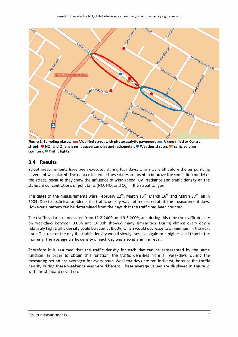
3 Street measurements The street measurements have been executed in the Castorweg, Hengelo (NL). Hengelo is a relatively small city in the east of the Netherlands. The Castorweg is not a main connection route, but relatively busy for a side street. One part of the street will be paved with air purifying pavement and another part will remain in the current condition (see Figure 1), and thus function as a control street, to compare the results of the air purifying pavement with the current situation. In both parts of the street measurement are executed to determine the variables as described in paragraph 3.1. These measurements are executed following a protocol (Ballari et al., 2008) which is made to ensure the reliability of the measurements. During this project, measurements have been executed on four days, all before the air purifying pavement was placed. During these days the variables that will be discussed in paragraph 3.1 have been measured from at least 9:00h to 16:00h.
3.1 Monitoring variables The following variables are measured in the Castorweg, according to the protocol mentioned before. UV and solar irradiance The UV irradiance is the direct energy source for the degradation process. It is measured at the surface of the street, with an interval of 5 minutes during the measuring days, using the UV‐radiometer. The total solar irradiance is measured every minute by the weather station. Relative Humidity (RH) Water molecules can compete with NOx particles for the active sites in the photocatalyst, making the degradation process less effective. However some amount of humidity is needed to form •OH radicals that fuel the degradation process. The relative humidity is measured by the weather station. Wind speed and direction In order to obtain reliable results, the measuring days have been mostly planned on days when the wind direction was perpendicular to the street. This way, the sources of the NOx concentrations that are measured are mainly automobiles in the Castorweg itself, which can be modelled by a diffusion‐convection equation in the mass balance. If the wind direction is more parallel to the street, the inlet and outlet conditions change, because pollution from adjacent streets flows towards or even through the measurement street, and pollution from traffic within the measurement street is blown away. The wind speed is also expected to have an influence on the background concentration of NOx gases. The higher the wind speed, in any direction, the higher the dispersion rate. Both the wind speed and direction are measured by the weather station at 5 m height. Traffic Traffic is the main source of pollution. In the measurement street a radar traffic counter measures and distinguishes all motorbikes, cars, busses and trucks that pass through the street. NOx concentration The concentration of NOx that is already present is an important factor in the degradation process. With a higher NOx concentration, the street surface adsorbs a larger amount of NOx particles, which increases the degradation process, and influences homogeneous atmospheric reactions in the form of the Leighton cycle which will be discussed in paragraph 4.3.3. The NOx concentration at each location is measured at three different heights (5, 30 and 150cm) above street level, to be able to determine the influence of the DeNOx pavement at these heights, the breathing height being

Simulation model for NOx distributions in a street canyon with air purifying pavement
Street measurements 6
represented by the measurements at 150cm. The passive tubes are also installed at the height of 150cm. O3 concentration The concentration of O3 (ozone) in the atmosphere can function as an indicator for the NOx concentration. It is used to determine the reaction rate constants for the Leighton cycle (paragraph 4.3.3).
3.2 Equipment In order to measure the instantaneous NOx concentration, two NOx analyzers are used. The NOx concentration is measured by an Ambient NOx Monitor Horiba APNA – 370 and an APNA ‐ 360. The APNA 370 always is stationed in the modified part of the street. The other analyzer alternates measuring in the control street and the background locations as follows: from 9:00h – 9:30h and from 15:30h – 16:00h it measures in the background, and in between these times it measures in the control street. The results from the NOx measurements in the background streets give a good indication of the background concentration of NOx. The NOx analyzers give the NOx concentrations in ppm, or parts per million. These concentrations can be expressed in mol/m3 by dividing the values in ppm by 22700, which is the volume in m3 of 106 molecules of air for standard pressure and room temperature. Besides the NOx analyzers, the average NOx concentration is measured by passive tubes that are installed at several locations along the Castorweg and in the background. The results of these passive tubes can verify measurements from the NOx analyzers and give an overview of the average NOx
concentration over a period of 3 weeks instead of just the instantaneous concentration. The average concentrations of NO and NO2 are measured by passive tubes: Gradko DIF 150 RTU. The average concentration of O3 is measured by another passive tube: Gradko DIF 300 RTU. Weather variables are measured by a Vantage Pro2 Wireless Weather Station, which can measure temperature, wind speed and direction, air pressure, relative humidity, solar irradiance and precipitation. Traffic is counted by a radar traffic counter. The instantaneous O3 concentration is measured manually using an Aeroqual Series 500 Multi‐Sensor Handheld Gas Monitor. The UV‐irradiance at the street surface is measured each 5 minutes using a UV‐VIS Radiometer RM‐12 Dr. Groebel UV‐Elektronik GmbH.
3.3 Sampling locations The locations of the different measurements are given in Figure 1. The weather station is attached to a lamp post at a height of 5m The NOx and O3 analyzers measured at heights of 5 cm, 30 cm and 1,50 m. The passive tubes are placed at a height of 1,50 m and the traffic counter is placed at a height of 2 m. A radiometer is used to measure the UV irradiance at street level.
Simulation model for NOx distributions in a street canyon with air purifying pavement
Street measurements 7
Figure 1: Sampling places. Modified street with photocatalytic pavement Unmodified or Control street. NOx and O3 analyzer, passive samples and radiometer. Weather station. Traffic volume counters. Traffic lights.
3.4 Results Street measurements have been executed during four days, which were all before the air purifying pavement was placed. The data collected at these dates are used to improve the simulation model of the street, because they show the influence of wind speed, UV irradiance and traffic density on the standard concentrations of pollutants (NO, NO2 and O3) in the street canyon. The dates of the measurements were February 12th, March 13th, March 16th and March 17th, all in 2009. Due to technical problems the traffic density was not measured at all the measurement days. However a pattern can be determined from the days that the traffic has been counted. The traffic radar has measured from 12‐2‐2009 until 9‐3‐2009, and during this time the traffic density on weekdays between 9:00h and 16:00h showed many similarities. During almost every day a relatively high traffic density could be seen at 9:00h, which would decrease to a minimum in the next hour. The rest of the day the traffic density would slowly increase again to a higher level than in the morning. The average traffic density of each day was also at a similar level. Therefore it is assumed that the traffic density for each day can be represented by the same function. In order to obtain this function, the traffic densities from all weekdays, during the measuring period are averaged for every hour. Weekend days are not included, because the traffic density during these weekends was very different. These average values are displayed in Figure 2, with the standard deviation.

Simulation model for NOx distributions in a street canyon with air purifying pavement
Street measurements 8
Figure 2: Average traffic density from 12‐2‐2009 to 9‐3‐2009 between 9:00h and 16:00h In order to process these data in the simulation model, a 2nd order polynomial function is drawn to fit the data. This function, represented by the black line, will be used to represent the traffic density for the street model, and is presented below:
69)9(9072.0 2 +−⋅= tTr (1) Where Tr is the traffic density [vehicles/h] t is the time of day [h] The R2 value for this function is 0.651, indicating that the 2nd order function describes the measured traffic density accurately enough for this project, because only the average traffic densities will be used in the street model and, as will be explained later, small variations in the traffic density do not have a significant influence on the pollutant concentrations in the street. The most important measurement results are displayed in the next sections for each of these days. For every measurement day the following variables are displayed:
‐ The pollutant concentrations in the Castorweg. These include the NO, NO2 and O3 concentrations
‐ The pollutant concentrations that were measured by rural RIVM stations in Hellendoorn and Eibergen during the measurement days (RIVM, 2009)
‐ The background pollutant concentrations in the morning and late in the afternoon ‐ The UV irradiance measured at the street surface and the solar irradiance measured
by the weather station in the Castorweg ‐ The wind speed and direction as measured by the weather station
Only the results from 9:00h to 16:00h will be used in the simulation model of the street. Note that in the graphs for the pollutant concentrations in paragraph 3.4.1 to 3.4.4 the NOx values can be read at the y‐axis on the left‐hand side, while the O3 values can be read at the right‐hand side. It is assumed that the O3 concentrations at 9:00h in the background street are equal to the O3 concentrations in the street at the same time, because there was only one O3 analyzer available.
Simulation model for NOx distributions in a street canyon with air purifying pavement
Street measurements 9
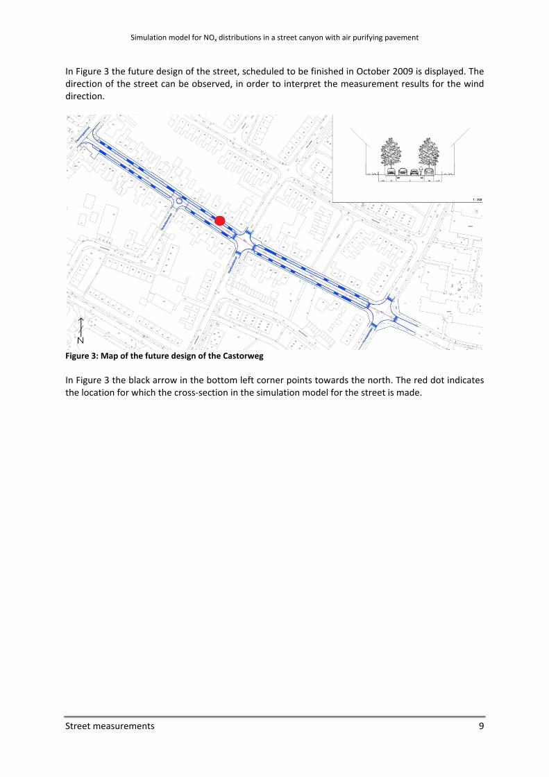
In Figure 3 the future design of the street, scheduled to be finished in October 2009 is displayed. The direction of the street can be observed, in order to interpret the measurement results for the wind direction.
Figure 3: Map of the future design of the Castorweg In Figure 3 the black arrow in the bottom left corner points towards the north. The red dot indicates the location for which the cross‐section in the simulation model for the street is made.

Simulation model for NOx distributions in a street canyon with air purifying pavement
Street measurements 10
3.4.1 Results from 12‐2‐2009 The weather on this measurement day was relatively sunny, with clouds in the afternoon. The average relative humidity was approximately 75%, and the average temperature was 2 °C. In Figure 4 the concentrations of NO, NO2 and O3 are displayed. It can be seen that the O3 level starts out very low and increases during the morning, stabilizing to a higher value in the afternoon. This is comparable to the O3 concentrations that were measured on 13‐3‐2009 (see Figure 7) and 17‐3‐2009 (see Figure 13). The NOx concentrations show an opposite behaviour, starting out relatively high and decreasing to a lower value during the morning. The O3 concentration measured by RIVM is approximately 25% lower than in the street. The NO and NO2 concentrations in the street and at RIVM are approximately the same, except in the morning when the concentrations in the street are significantly higher. This can be explained by the fact that RIVM measures the concentrations in a rural area with less traffic than in the Castorweg. An increase in the NOx concentration in the afternoon can be seen, which can at least partly be attributed to the lower irradiance in the afternoon, with a consequential decrease in the atmospheric reactions that will be discussed in paragraph 4.3.3.
Figure 4: Pollutant concentrations in the street (full lines) and measured by RIVM (dotted lines) on 12‐2‐2009 At 9:00h in the background street, the NO concentration was 9.78*10‐7 mol/m3 and the NO2 concentration was 1.33*10‐6 mol/m3.
09:00 10:00 11:00 12:00 13:00 14:00 15:00 16:000.00
0.02
0.04
0.06
0.08
0.10
0.00
0.01
0.02
0.03
0.04
0.05
0.06
O3 C
once
ntra
tion
(ppm
)
NO 131 NO RIVM NO2 131 NO2 RIVM
Time (hh:mm)
Con
cent
ratio
n (p
pm)
O3 O3 RIVM

Simulation model for NOx distributions in a street canyon with air purifying pavement
Street measurements 11
In Figure 5 it can be observed that both the UV and the total irradiance increased during the morning. In the afternoon more clouds drifted over the street, causing the strong variations in the measured irradiance. Later in the afternoon the maximum irradiance decreased again, which is normal for the month of February. The shapes of the UV and total irradiance curve are similar. The solar irradiance shows more fluctuations than the UV irradiance, because the solar irradiance is measured every minute, while the UV irradiance is only measured every 5 minutes.
The wind speed and direction for this measurement day are displayed in Figure 6.The direction of the points in the graph shows the wind direction, and the distance from the center of the graph is a measure for the wind speed in that direction. It can be observed that the average wind direction was WNW, which is almost parallel to the street. The average wind speed on this day was 1.53 m/s.
Figure 6: Wind speed (m/s) and direction on 12‐2‐2009
09:00 10:00 11:00 12:00 13:00 14:00 15:00 16:00 17:000
2
4
6
8
10
12
UV
(W m
-2)
Time (hh:mm)
0
1
2
3
4
5
6N
NE
E
SE
S
SW
W
NW
0
1
2
3
4
5
6
Win
d S
peed
(m/s
)
09:00 10:00 11:00 12:00 13:00 14:00 15:00 16:00 17:000
100
200
300
400
500
600
Sola
r rad
iatio
n (W
m-2)
Time (hh:mm)
Figure 5: UV radiation (left) and solar radiation (right) in W/m2 on 12‐2‐2009
Simulation model for NOx distributions in a street canyon with air purifying pavement
Street measurements 12
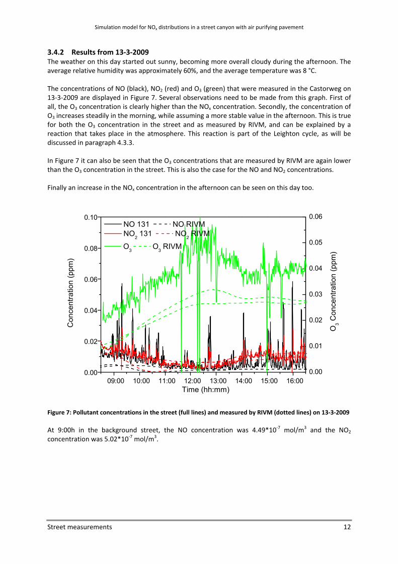
3.4.2 Results from 13‐3‐2009 The weather on this day started out sunny, becoming more overall cloudy during the afternoon. The average relative humidity was approximately 60%, and the average temperature was 8 °C. The concentrations of NO (black), NO2 (red) and O3 (green) that were measured in the Castorweg on 13‐3‐2009 are displayed in Figure 7. Several observations need to be made from this graph. First of all, the O3 concentration is clearly higher than the NOx concentration. Secondly, the concentration of O3 increases steadily in the morning, while assuming a more stable value in the afternoon. This is true for both the O3 concentration in the street and as measured by RIVM, and can be explained by a reaction that takes place in the atmosphere. This reaction is part of the Leighton cycle, as will be discussed in paragraph 4.3.3. In Figure 7 it can also be seen that the O3 concentrations that are measured by RIVM are again lower than the O3 concentration in the street. This is also the case for the NO and NO2 concentrations. Finally an increase in the NOx concentration in the afternoon can be seen on this day too.
Figure 7: Pollutant concentrations in the street (full lines) and measured by RIVM (dotted lines) on 13‐3‐2009 At 9:00h in the background street, the NO concentration was 4.49*10‐7 mol/m3 and the NO2 concentration was 5.02*10‐7 mol/m3.
09:00 10:00 11:00 12:00 13:00 14:00 15:00 16:000.00
0.02
0.04
0.06
0.08
0.10
0.00
0.01
0.02
0.03
0.04
0.05
0.06
O3 C
once
ntra
tion
(ppm
)
NO 131 NO RIVM NO2 131 NO2 RIVM
Time (hh:mm)
Con
cent
ratio
n (p
pm)
O3 O3 RIVM

Simulation model for NOx distributions in a street canyon with air purifying pavement
Street measurements 13
In Figure 8 the UV irradiance as measured at the street surface and the total solar irradiance are displayed. It can be clearly seen that the irradiance starts at a low level in the morning and increases to a maximum around noon, after which it decreases again. This is to be expected in a normal sunny day. It can also be seen that the shape of the UV and solar irradiance is approximately similar, with the amount of UV irradiance being a fraction of the total solar irradiance. The maximum solar irradiance is approximately 600 W/m2, which indicates a sunny day for the month of March.
Figure 8: UV irradiance (left) and solar irradiance (right) in W/m2 on 13‐3‐2009 In Figure 9 the wind speed and direction are displayed. It can be seen that the average wind direction was SW (south‐west) or SSW. This is approximately perpendicular to the street. The average wind speed that was measured on that day was 1.35 m/s.
Figure 9: Wind speed (m/s) and direction on 13‐3‐2009
09:00 10:00 11:00 12:00 13:00 14:00 15:00 16:000
2
4
6
8
10
12
14
16
18
UV
(W m
-2)
Time (hh:mm)09:00 10:00 11:00 12:00 13:00 14:00 15:00 16:00
0
100
200
300
400
500
600
700
800
900
Sola
r rad
iatio
n (W
m-2)
Time (hh:mm)
0
1
2
3
4
5
6N
NE
E
SE
S
SW
W
NW
0
1
2
3
4
5
6
Win
d S
peed
(m/s
)

Simulation model for NOx distributions in a street canyon with air purifying pavement
Street measurements 14
3.4.3 Results from 16‐3‐2009 The weather this day was completely cloudy. The average relative humidity was approximately 55%, and the average temperature was 7 °C. In Figure 10 the pollutant concentrations are displayed. It can be seen that the O3 concentration is again higher than the NOx concentration for the greater part of the day. Unlike the last day, the O3 concentration in the street only gradually increases a little during the day, and has approximately the same value as the O3 concentrations that were measured by RIVM. The NOx concentrations are again a little higher in the street than at the RIVM measuring points, with much higher peaks which can be contributed to passing traffic. The small increase in O3 levels can be attributed to the low irradiance for this day. The atmospheric reactions that are fuelled by UV irradiance are not taking place as much as on the other measurement days.
Figure 10: Pollutant concentrations in the street (full lines) and measured by RIVM (dotted lines) on 16‐3‐2009 At 9:00h in the background street, the NO concentration was 1.23*10‐7 mol/m3 and the NO2 concentration was 3.35*10‐7 mol/m3.
09:00 10:00 11:00 12:00 13:00 14:00 15:00 16:000.00
0.02
0.04
0.06
0.08
0.10
0.00
0.01
0.02
0.03
0.04
0.05
0.06
NO 131 NO RIVM NO2 131 NO2 RIVM
O3 C
once
ntra
tion
(ppm
)
Time (hh:mm)
Con
cent
ratio
n (p
pm)
O3 O3 RIVM
Simulation model for NOx distributions in a street canyon with air purifying pavement
Street measurements 15
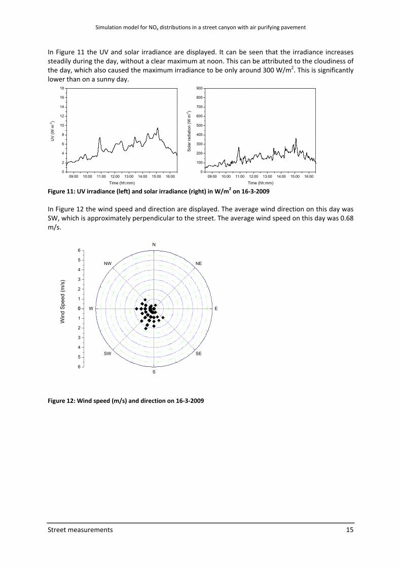
In Figure 11 the UV and solar irradiance are displayed. It can be seen that the irradiance increases steadily during the day, without a clear maximum at noon. This can be attributed to the cloudiness of the day, which also caused the maximum irradiance to be only around 300 W/m2. This is significantly lower than on a sunny day.
Figure 11: UV irradiance (left) and solar irradiance (right) in W/m2 on 16‐3‐2009 In Figure 12 the wind speed and direction are displayed. The average wind direction on this day was SW, which is approximately perpendicular to the street. The average wind speed on this day was 0.68 m/s.
Figure 12: Wind speed (m/s) and direction on 16‐3‐2009
09:00 10:00 11:00 12:00 13:00 14:00 15:00 16:000
2
4
6
8
10
12
14
16
18
UV
(W m
-2)
Time (hh:mm)09:00 10:00 11:00 12:00 13:00 14:00 15:00 16:00
0
100
200
300
400
500
600
700
800
900
Sola
r rad
iatio
n (W
m-2)
Time (hh:mm)
0
1
2
3
4
5
6N
NE
E
SE
S
SW
W
NW
0
1
2
3
4
5
6
Win
d S
peed
(m/s
)

Simulation model for NOx distributions in a street canyon with air purifying pavement
Street measurements 16
3.4.4 Results from 17‐3‐2009 The weather on this day started out partially sunny and after a cloudy period around noon it changed to sunny with clouds drifting by. The average relative humidity was approximately 50%, and the average temperature was 9°C. In Figure 13 the pollutant concentrations are displayed and they are comparable to the concentrations that were measured on 13‐3‐2009 (see Figure 7).
Figure 13: Pollutant concentrations in the street (full lines) and measured by RIVM (dotted lines) on 17‐3‐2009 At 9:00h in the background street, the NO concentration was 1.72*10‐6 mol/m3 and the NO2 concentration was 1.00*10‐6 mol/m3.
09:00 10:00 11:00 12:00 13:00 14:00 15:00 16:000.00
0.02
0.04
0.06
0.08
0.10
0.00
0.01
0.02
0.03
0.04
0.05
0.06 NO 126 NO RIVM NO2 126 NO2 RIVM
O3 C
once
ntra
tion
(ppm
)
Time (hh:mm)
Con
cent
ratio
n (p
pm)
O3 O3 RIVM
Simulation model for NOx distributions in a street canyon with air purifying pavement
Street measurements 17
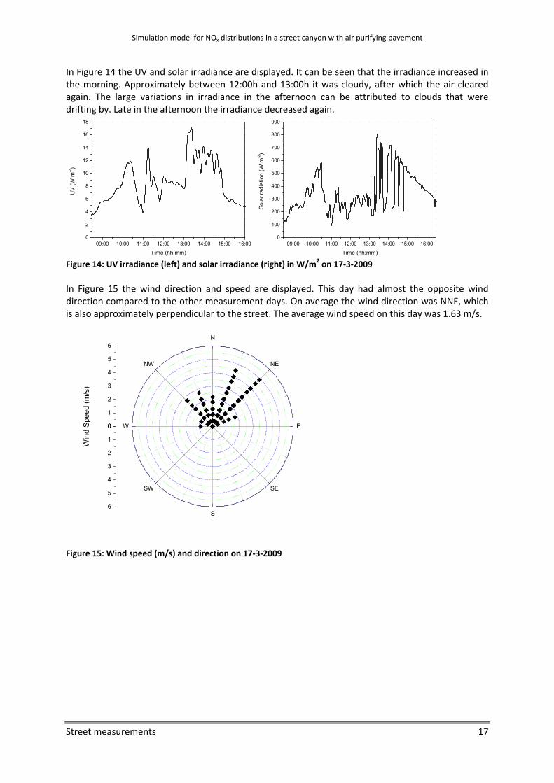
In Figure 14 the UV and solar irradiance are displayed. It can be seen that the irradiance increased in the morning. Approximately between 12:00h and 13:00h it was cloudy, after which the air cleared again. The large variations in irradiance in the afternoon can be attributed to clouds that were drifting by. Late in the afternoon the irradiance decreased again.
Figure 14: UV irradiance (left) and solar irradiance (right) in W/m2 on 17‐3‐2009 In Figure 15 the wind direction and speed are displayed. This day had almost the opposite wind direction compared to the other measurement days. On average the wind direction was NNE, which is also approximately perpendicular to the street. The average wind speed on this day was 1.63 m/s.
Figure 15: Wind speed (m/s) and direction on 17‐3‐2009
09:00 10:00 11:00 12:00 13:00 14:00 15:00 16:000
2
4
6
8
10
12
14
16
18
UV
(W m
-2)
Time (hh:mm)09:00 10:00 11:00 12:00 13:00 14:00 15:00 16:00
0
100
200
300
400
500
600
700
800
900
Sola
r rad
iatio
n (W
m-2)
Time (hh:mm)
0
1
2
3
4
5
6N
NE
E
SE
S
SW
W
NW
0
1
2
3
4
5
6
Win
d S
peed
(m/s
)

Simulation model for NOx distributions in a street canyon with air purifying pavement
Street measurements 18
3.5 Conclusions Solar and UV irradiance In Figure 5, Figure 8, Figure 11 and Figure 14 it can be clearly seen that the UV irradiance and total solar irradiance show the same behavior throughout the measuring days. Therefore the assumption is made that the UV irradiance that reaches the street surface is proportional to the total solar irradiance, within the range of these measurements. Based on these measurements the UV irradiance that reaches the street surface can be assessed to be 2.5% of the total solar irradiance. Pollutant concentrations In general the concentrations of all pollutants that were measured in a rural area by RIVM are lower than the concentrations in the street. This can be attributed to a higher traffic density in the street. It can be seen in Figure 7, Figure 10 and Figure 13 that the O3 concentrations in the street as well as measured by RIVM show a tendency to increase in the morning and stabilize in the afternoon. NO and NO2 however show a tendency to decrease in the morning. The increase in O3 is much higher for days with higher irradiance, which can be attributed to the Leighton cycle. This cycle which produces and degrades O3, NO and NO2 under the influence of UV irradiance will be discussed in paragraph 4.3.3. Wind During the measurement days the wind direction and speed were not completely constant, as can be seen in Figure 6, Figure 9, Figure 12 and Figure 15. However for most of the days the wind direction was approximately perpendicular to the street canyon, and for the simulation model of the street a constant wind direction and speed will be used. Traffic density As explained before, the traffic density was not measured at some measurement days. However there was a fair amount of traffic data for other days available that showed a common behavior. This behavior is described with a common function for the traffic density during the day, and this will be used for the simulation model of the street.

Simulation model for NOx distributions in a street canyon with air purifying pavement
Simulation model 19
4 Simulation model In this chapter the requirements for the simulation of a wind flow profile and the pollutant concentrations are presented. In order to model these properties, Comsol Multiphysics is used. This software will be discussed in paragraph 4.1. The requirements for the simulation of the wind flow profile are presented in paragraph 4.2 and the requirements regarding the pollutant concentrations are discussed in paragraph 4.3. In order to make the simulation model as accurate as possible, several parts are needed. The Castorweg, where the air purifying pavement will be placed, is represented by a (2‐dimensional) cross section of the street canyon at the measuring point described in chapter 3 (see Figure 3). In order to determine the effect of the wind on the NOx concentrations and the air purifying pavement a wind flow profile must be developed. The traffic is represented by a car exhaust term within the street canyon. The air purifying pavement is represented by a series of reactions that take place at the street surface, based on a kinetic that is described in paragraph 4.3.2 and laboratory experiments. A complicating factor in this model is a natural reaction cycle between NO, NO2 and O3 that should be modelled correctly for an accurate simulation model of the Castorweg.
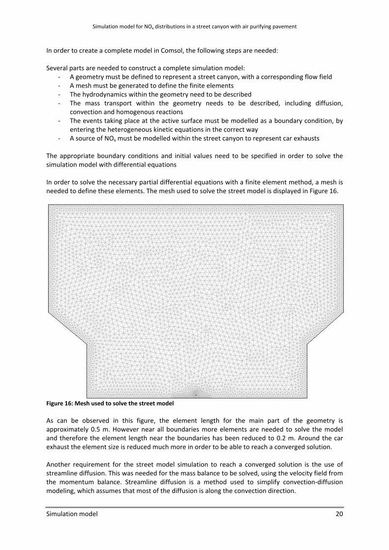
4.1 Comsol The software used to create simulation models of the reactor and the street is Comsol Multiphysics 3.5. This program uses separate modules to describe different physical or chemical phenomena. These modules can have common variables, thus coupling the modules and creating an integral multiphysics model. All simulation models in this project are 2‐dimensional (2D). Comsol Multiphysics is based on partial differential equations (PDE’s), which can be solved numerically by a finite element method, by giving the appropriate initial and boundary conditions. It uses a mesh of finite elements to reach a converged solution in an iterative process (see Figure 16). The size of the elements as well as the PDE’s themselves can be changed within the program. However a large selection of PDE’s is pre‐programmed in different modules and can be used and combined instantly. For this project two modules are used. The first module describes a steady state wind velocity profile in the case of the street model, based on a constant average wind speed, perpendicular to the street canyon. Steady state modelling is based on situations where equilibrium is reached. For the wind flow profile this is assumed to be sufficient, in order not to complicate the simulation model. A stationary segregated solver is used to obtain the steady state solution. A steady state plug flow profile is used to describe the flow through the reactor. The second module describes the NOx and O3 concentrations within the desired geometry. Two different models are made in this project, of which the first is a simulation model of the reactor that is used in the laboratory experiments. This model is based on a steady state mass balance, because the conditions in the lab are controlled and constant for each measurement. For the street model however a transient model is used to determine the pollutant concentrations during a day. A transient model describes a situation that changes over time, and in this case the model simulates a day between 9:00h and 16:00h. By using this transient model, variables such as car emissions, solar irradiance and background concentrations, can be changed in the course of this day. The solution for this transient model is obtained using a time dependent solver. The two modules can be coupled by first solving the wind flow profile separately, and using that velocity profile as input in the transient module to solve all concentrations.
Simulation model for NOx distributions in a street canyon with air purifying pavement
Simulation model 20
In order to create a complete model in Comsol, the following steps are needed: Several parts are needed to construct a complete simulation model:
‐ A geometry must be defined to represent a street canyon, with a corresponding flow field ‐ A mesh must be generated to define the finite elements ‐ The hydrodynamics within the geometry need to be described ‐ The mass transport within the geometry needs to be described, including diffusion,
convection and homogenous reactions ‐ The events taking place at the active surface must be modelled as a boundary condition, by
entering the heterogeneous kinetic equations in the correct way ‐ A source of NOx must be modelled within the street canyon to represent car exhausts
The appropriate boundary conditions and initial values need to be specified in order to solve the simulation model with differential equations In order to solve the necessary partial differential equations with a finite element method, a mesh is needed to define these elements. The mesh used to solve the street model is displayed in Figure 16.
Figure 16: Mesh used to solve the street model As can be observed in this figure, the element length for the main part of the geometry is approximately 0.5 m. However near all boundaries more elements are needed to solve the model and therefore the element length near the boundaries has been reduced to 0.2 m. Around the car exhaust the element size is reduced much more in order to be able to reach a converged solution. Another requirement for the street model simulation to reach a converged solution is the use of streamline diffusion. This was needed for the mass balance to be solved, using the velocity field from the momentum balance. Streamline diffusion is a method used to simplify convection‐diffusion modeling, which assumes that most of the diffusion is along the convection direction.

Simulation model for NOx distributions in a street canyon with air purifying pavement
Simulation model 21
In order to solve the momentum balance for high inlet velocities, this module was first solved for lower inlet velocities, after which this solution was stored and used to solve the momentum balance for higher inlet velocities. The hydrodynamic equations that describe the momentum balance will be discussed in paragraph 4.2. Convection, diffusion, reaction rates and source terms for NOx are modelled by mass transport equations, which will be discussed in paragraph 4.3.
4.2 Hydrodynamics In this paragraph the general hydrodynamics of both the reactor and the street model are described. For a laminar flow, as is present in the reactor, only the Navier‐Stokes equation is needed, which apply for all flows. The flow through the street canyon will be modelled as a turbulent flow, which is also described by the Navier‐Stokes equation. However for a turbulent flow this equation needs to be augmented with equations that describe the turbulent behaviour of the flow. In order to determine the turbulence of a flow the Reynolds number can be used, which is given in paragraph 4.2.1. In paragraph 4.2.2 the Navier‐Stokes equation is described, and in paragraph 4.2.3 the turbulence equations (as used by Comsol) describing the turbulent energy and the turbulent dissipation rate are given. The boundary conditions needed to solve the differential equations differ in the reactor and the street; therefore they are given in chapter 5 and 6 respectively.
4.2.1 Reynolds number The turbulence of the flow is defined by the Reynolds number (Re), which is calculated as follows:
ηρ Lu ⋅⋅
= 0Re (2)
with ρ = density of the medium [kg/m3] u0 = mean velocity [m/s] L = representative length [m] η = viscosity of the medium [Pa*s] Normally, a flow is laminar if Re < 2000, and if Re > 3000, the flow is turbulent. In paragraph 5.2 and 6.2 respectively, the Reynolds number is calculated for the flow through the reactor and the street canyon.
Simulation model for NOx distributions in a street canyon with air purifying pavement
Simulation model 22
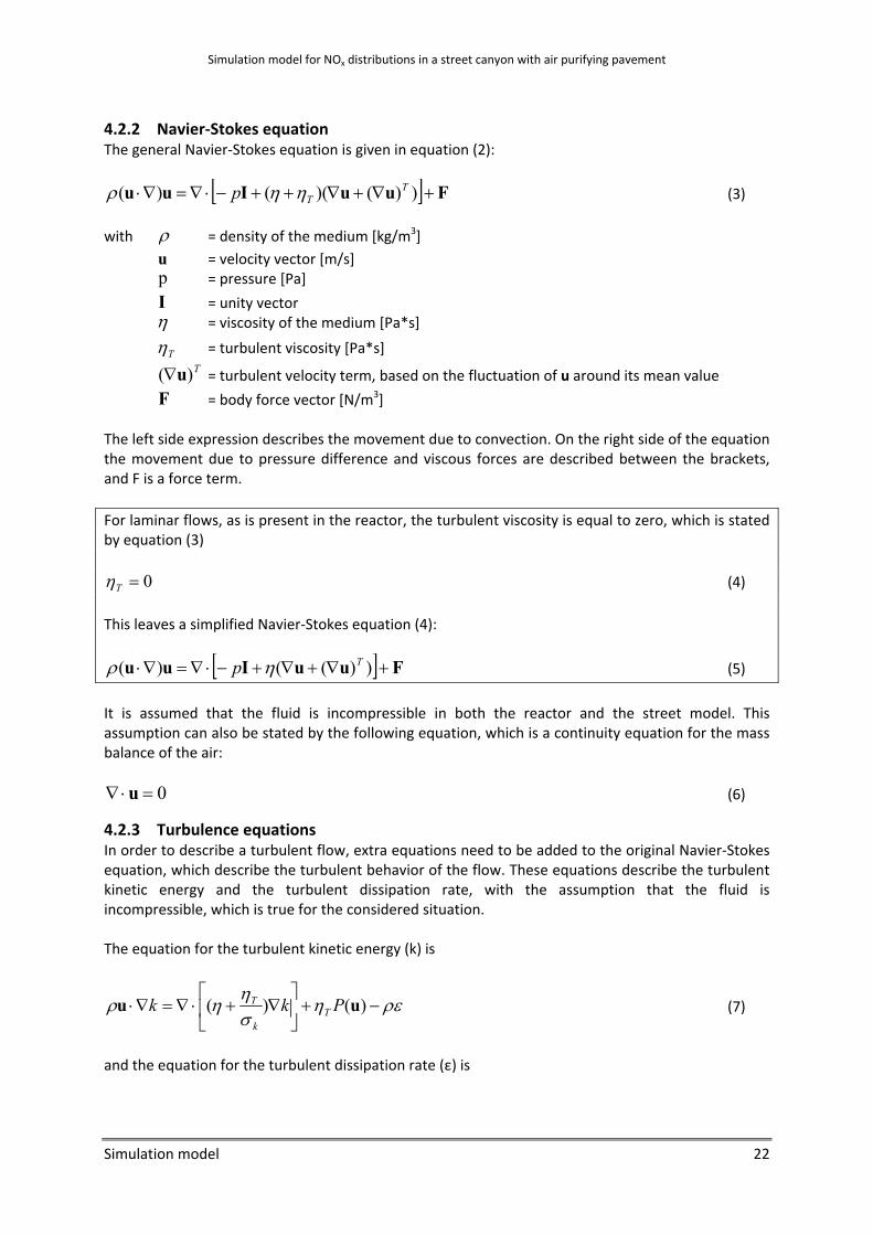
4.2.2 Navier‐Stokes equation The general Navier‐Stokes equation is given in equation (2):
[ ] FuuIuu +∇+∇++−⋅∇=∇⋅ ))()(()( TTp ηηρ (3)
with ρ = density of the medium [kg/m3] u = velocity vector [m/s]
p = pressure [Pa]
I = unity vector η = viscosity of the medium [Pa*s]
Tη = turbulent viscosity [Pa*s]
T)( u∇ = turbulent velocity term, based on the fluctuation of u around its mean value
F = body force vector [N/m3] The left side expression describes the movement due to convection. On the right side of the equation the movement due to pressure difference and viscous forces are described between the brackets, and F is a force term. For laminar flows, as is present in the reactor, the turbulent viscosity is equal to zero, which is stated by equation (3)
0=Tη (4) This leaves a simplified Navier‐Stokes equation (4):
[ ] FuuIuu +∇+∇+−⋅∇=∇⋅ ))(()( Tp ηρ (5)
It is assumed that the fluid is incompressible in both the reactor and the street model. This assumption can also be stated by the following equation, which is a continuity equation for the mass balance of the air:
0=⋅∇ u (6)
4.2.3 Turbulence equations In order to describe a turbulent flow, extra equations need to be added to the original Navier‐Stokes equation, which describe the turbulent behavior of the flow. These equations describe the turbulent kinetic energy and the turbulent dissipation rate, with the assumption that the fluid is incompressible, which is true for the considered situation. The equation for the turbulent kinetic energy (k) is
ρεηση
ηρ −+⎥⎦
⎤⎢⎣
⎡∇+⋅∇=∇⋅ )()( uu Pkk T
k
T (7)
and the equation for the turbulent dissipation rate (ε) is
Simulation model for NOx distributions in a street canyon with air purifying pavement
Simulation model 23
kC
kPC TT
221 )(
)(ρεεη
εση
ηερ εε
ε
−+⎥⎦
⎤⎢⎣
⎡∇+⋅∇=∇⋅
uu (8)
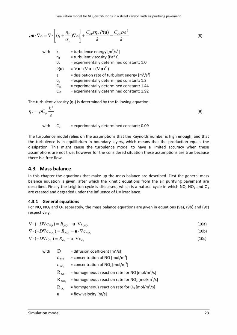
with k = turbulence energy [m2/s2]
ηT = turbulent viscosity [Pa*s] σk = experimentally determined constant: 1.0
P(u) = ))((: Tuuu ∇+∇∇ ε = dissipation rate of turbulent energy [m2/s3] σε = experimentally determined constant: 1.3 Cε1 = experimentally determined constant: 1.44 Cε2 = experimentally determined constant: 1.92 The turbulent viscosity (ηT) is determined by the following equation:
ερη μ
2kCT = (9)
with Cμ = experimentally determined constant: 0.09 The turbulence model relies on the assumptions that the Reynolds number is high enough, and that the turbulence is in equilibrium in boundary layers, which means that the production equals the dissipation. This might cause the turbulence model to have a limited accuracy when these assumptions are not true; however for the considered situation these assumptions are true because there is a free flow.
4.3 Mass balance In this chapter the equations that make up the mass balance are described. First the general mass balance equation is given, after which the kinetic equations from the air purifying pavement are described. Finally the Leighton cycle is discussed, which is a natural cycle in which NO, NO2 and O3 are created and degraded under the influence of UV irradiance.
4.3.1 General equations For NO, NO2 and O3 separately, the mass balance equations are given in equations (9a), (9b) and (9c) respectively.
NONONO cRcD ∇⋅−=∇−⋅∇ u)( (10a)
222)( NONONO cRcD ∇⋅−=∇−⋅∇ u (10b)
333)( OOO cRcD ∇⋅−=∇−⋅∇ u (10c)
with D = diffusion coefficient [m2/s]
NOc = concentration of NO [mol/m3]
2NOc = concentration of NO2 [mol/m3]
NOR = homogeneous reaction rate for NO [mol/m3/s]
2NOR = homogeneous reaction rate for NO2 [mol/m3/s]
3OR = homogeneous reaction rate for O3 [mol/m3/s]
u = flow velocity [m/s]
Simulation model for NOx distributions in a street canyon with air purifying pavement
Simulation model 24
The left‐side expression describes diffusion, R describes the homogeneous reaction rate as a source or sink of NOx or O3 and the remainder of the right‐side expression describes convection. The total mass balance equation states that for each volume element, the change in NOx or O3 concentration is equal to the production in this volume subtracted by the amount that is lost by diffusion and convection. The homogeneous reaction rate will be determined by the Leighton cycle, which is explained in paragraph 4.3.3. The flow velocity in this mass balance is determined by the hydrodynamic equations from the momentum balance module.
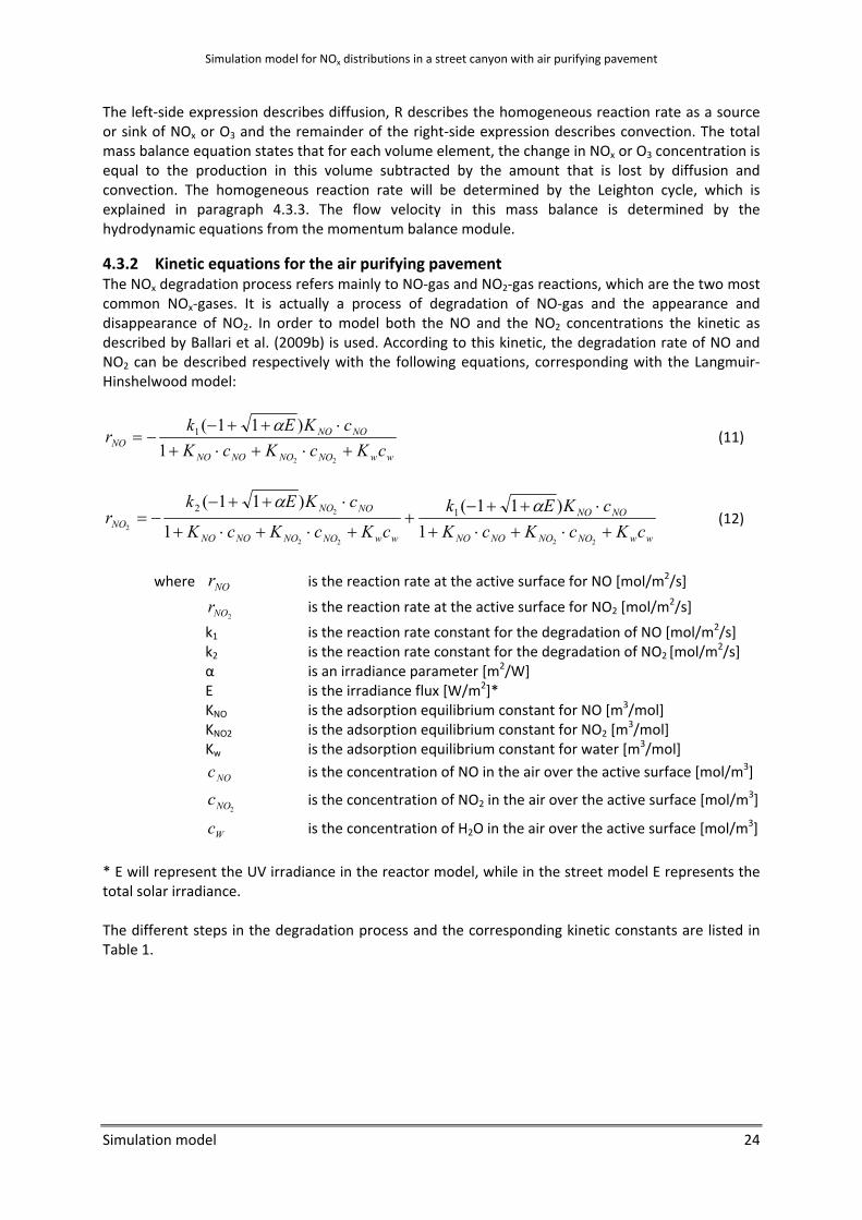
4.3.2 Kinetic equations for the air purifying pavement The NOx degradation process refers mainly to NO‐gas and NO2‐gas reactions, which are the two most common NOx‐gases. It is actually a process of degradation of NO‐gas and the appearance and disappearance of NO2. In order to model both the NO and the NO2 concentrations the kinetic as described by Ballari et al. (2009b) is used. According to this kinetic, the degradation rate of NO and NO2 can be described respectively with the following equations, corresponding with the Langmuir‐ Hinshelwood model:
wwNONONONO
NONONO cKcKcK
cKEkr
+⋅+⋅+⋅++−
−=22
1)11(1 α
(11)
wwNONONONO
NONO
wwNONONONO
NONONO cKcKcK
cKEkcKcKcK
cKEkr
+⋅+⋅+⋅++−
++⋅+⋅+
⋅++−−=
2222
2
2 1)11(
1
)11(12 αα
(12)
where NOr is the reaction rate at the active surface for NO [mol/m2/s]
2NOr is the reaction rate at the active surface for NO2 [mol/m2/s]
k1 is the reaction rate constant for the degradation of NO [mol/m2/s] k2 is the reaction rate constant for the degradation of NO2 [mol/m2/s]
α is an irradiance parameter [m2/W] E is the irradiance flux [W/m2]* KNO is the adsorption equilibrium constant for NO [m3/mol] KNO2 is the adsorption equilibrium constant for NO2 [m
3/mol] Kw is the adsorption equilibrium constant for water [m3/mol] NOc is the concentration of NO in the air over the active surface [mol/m3]
2NOc is the concentration of NO2 in the air over the active surface [mol/m3]
Wc is the concentration of H2O in the air over the active surface [mol/m3]
* E will represent the UV irradiance in the reactor model, while in the street model E represents the total solar irradiance. The different steps in the degradation process and the corresponding kinetic constants are listed in Table 1.

Simulation model for NOx distributions in a street canyon with air purifying pavement
Simulation model 25
Table 1: Overview of NOx degradation process The reaction rates described in equations (10) and (11) are implemented in Comsol as a flux over the active surface, with the direction perpendicular to this surface. The values for the parameters used in equations (10) and (11) were determined with laboratory experiments in a reactor (Ballari et al., 2009b), and are displayed in Table 2. The stone that was used to determine these parameters was produced by Marlux (Belgium) in 2005 and has a blue top layer. This type of stone was also used in Antwerp (Beeldens, 2007). Parameter Value k1 7.333*10‐8 mol/dm2/min k2 2.550*10‐6 mol/dm2/min KNO 7.610*104 m3/mol KNO2 3.570*104 m3/mol Kw 62 m3/mol α 0.276 m2/W (in the reactor model)
0.0069 m2/W (in the street model) Table 2: Parameter values used in the kinetic equations (11) and (12) Note that the value for α in the street model is 2.5% of the original value for α, as used in the reactor model, because α for the street model contains a conversion factor from total solar irradiance to only UV irradiance.
4.3.3 Leighton cycle At the start of this project it was assumed that the atmospheric reactions could be neglected. This changed however after some preliminary simulations, which were based on this assumption. They predicted the NOx concentrations well for days with low irradiance. However for high irradiance days, the simulated NOx concentrations were much higher than the measured values. With exception of the irradiance, all variables were approximately similar during the measurement days. In order to explain the differences between the simulation and the measurements, the measured ozone concentrations should be considered as well. These ozone concentrations showed, with several measurements, the opposite behaviour of NOx concentrations. When the irradiance increased, the concentration of ozone increased as well, whereas the NOx concentrations tended to decrease. This is most likely caused by the Leighton cycle, which is explained in this paragraph. In the atmosphere a process takes place in which NO, NO2 and O3 are both formed and destructed. Several sources (Bohn et al., 2005; Fowler et al., 1998; Ghormley et al., 1973; Kilifarska et al., 2005;

Simulation model for NOx distributions in a street canyon with air purifying pavement
Simulation model 26
Marsili‐Libelli, 1996 and Zafonte et al., 2002) agree that this process, which is called the “Leighton cycle”, starts with photolysis of NO2 or the degradation of NO2 under the influence of UV irradiance:
ONOnmhNO tJ +⎯→⎯±<+ )430(2 λν (13)
Where tJ is the reaction rate constant for the photolysis process, dependent on the amount
of UV irradiance [1/s] The O‐atoms created in this process then react instantaneously with O2 to form O3, and in an unpolluted atmosphere the NO reacts with O3 to form NO2 and O2 again:
32 OOO →+ (14)
2233 ONOONO k +⎯→⎯+ (15)
Where k3 is the reaction rate constant for the degradation of NO In unpolluted atmospheres, these reaction lead to the following equilibrium (Marsili‐Libelli, 1996):
2
3
3 NO
ONOt
ccc
kJ ⋅
= (16)
Equation 16 describes the pseudo‐steady‐state relationship between the three species under the influence of UV‐irradiance for an unpolluted atmosphere. In a more polluted atmosphere, more
reactions take place which disturb this balance. More radicals such as •OH and •2RO are available,
enabling the following reactions:
328 HNOOHNO k⎯→⎯+ • (17)
2212 NORONORO k +⎯→⎯+ •• (18)
Where k8 and k12 are the corresponding reaction rates for equations 17 and 18 respectively,
and HNO3 (nitric acid) causes acid rain NO2 is also degraded by a reaction with O3:
233210 ONOONO k +⎯→⎯+ (19)
The reaction in equation 19 occurs when there are significant concentrations of both NO2 and O3, and because it does not require light, it causes a depletion of O3 during the night, together with the reaction in equation 15. This nocturnal process causes NO and NO2 concentrations to be relatively high in the morning, while the O3 concentration is relatively low. During the day, the O3 is again created by photolysis and the Leighton cycle is repeated. Marsili‐Libelli (1996) proposes a simplified kinetic for the Leighton cycle, based on the assumption that the radical attack in equation (17) could be excluded. The daytime NO enhancement resulting from NO2 photolysis, as described in equation 13, was also excluded because it was observed that this produced the best fit. This could be explained by the overwhelming presence of free organic radicals, producing almost instant oxidation of NO into NO2 and concealing the Leighton reaction.

Simulation model for NOx distributions in a street canyon with air purifying pavement
Simulation model 27
The NO2 that is formed then bonds with organic pollutants such as CH3CO3 (peroxy acetyl) to form CH3CO3NO2 (peroxy‐acetyl‐nitrate), in a temperature dependent reversible equilibrium. For low temperatures, as generally present during the measurement days in Hengelo, the CH3CO3 functions as a sink for NO2. Over time, the CH3CO3NO2 is transported away, releasing the NO2 in other locations when the temperature increases. The net result of this last process is a disappearance of NO from the atmosphere in the street. The simplified kinetic as proposed by Marsili‐Libelli (1996) for the Leighton cycle consists of the following homogeneous reaction rates for NO, NO2 and O3 respectively:
NOONONO
NO ckcckdtdc
R ⋅−⋅⋅−== 123 3 (20)
NOONONOTNO
NO ckcckcJdtdc
R ⋅+⋅⋅+⋅−= 123 32
2
2 (21)
32
3
3 3 ONONOTO
O cckcJdtdc
R ⋅⋅−⋅== (22)
In order to complete the mass balance from these equations, it is assumed that the reaction rate for equation (15) that describes a degradation of NO is equal to the reaction rate for the reaction in which CH3CO3NO2 is formed from CH3CO3. According to Marsili‐Libelli, Jt is linearly dependent on the solar irradiance. This can be expressed with the following equation:
EJt ⋅= γ (23)
Where γ is a constant conversion factor, to be determined [m2/W/s] E is the total solar irradiance [W/m2] It is assumed that the UV‐part of the total solar irradiance is a constant, based on a comparison of simultaneous total solar irradiance and UV measurements. Approximately 2.5% of the total solar irradiance is UV. This is also considered in the constant γ. As explained earlier in this section, k3 and k12 are reaction rate constants, and Jt depends on the amount of solar irradiance. Marsili‐Libelli assumes a similar function for Jt for every day, which has the form of a cosine, with the maximum irradiance at noon. However in order to model the Leighton cycle for this street model more accurately for days with other irradiance patterns, such as cloudy days, another function is chosen to represent the solar irradiance. In this project actual solar irradiance data are used that have been collected on measurement days. The irradiance data from 9:00h until 16:00h of that day are graphed, and a 6th order polynomial equation is fitted to these data. This polynomial equation is then used to describe the solar irradiance during that day. In this way variations in the solar irradiance, caused by weather phenomena, are taken into account, and the modelling of the Leighton cycle is closer to the reality. The solar irradiance graphs with the polynomial equations for the measurement days can be found in appendix A. Besides the function for Jt, Marsili‐Libelli also deducted values for k3 and k12 using a smog chamber. However since this simulation model represents street circumstances these values were revised to better describe these conditions. The appropriate values for these reaction rate constants have been
Simulation model for NOx distributions in a street canyon with air purifying pavement
Simulation model 28
determined by an optimization process using the solver tool in Microsoft Excel, in which the NO, NO2 and O3 concentrations from an environment without sources were compared to the solar irradiance at that time. For the optimization process, pollutant concentrations from an area without contamination sources were needed to obtain the actual reaction rates of the Leighton cycle. These concentrations of NO, NO2 and O3 were taken from two RIVM measuring stations in Eibergen and Hellendoorn, which are the two closest rural measuring stations to Hengelo. The values from these measuring stations have been averaged. For the solar irradiance the polynomial equations as determined before were used. For this optimization process a total of six days of data were used, between February and June. The goal of this process was to minimize the error between the actual measurements and the model prediction by varying k3, k12 and γ. In Excel the concentrations of NO, NO2 and O3 were modelled using equations (8) to (11) and as initial values for these concentrations the RIVM concentrations were used. This way the RIVM data and the model data start at the same point. In Excel the solver tool was used to minimize the error between the model and the RIVM data for the measurement days between 9:00h and 16:00h, by varying the values of k3, k12 and γ. This process resulted in optimal values for these constants, which can be used later in the street model. The optimized values are displayed in Table 3. They are based on circumstances in the area around Hengelo in spring time, such as an average temperature around 280 K. Perhaps for other circumstances, with another temperature, the values of the reaction rate constants for the Leighton cycle could be different. constant value unit k3 1 m3/mol/s k12 1.55*10‐4 1/s γ 3.12*10‐7 m2/W/s Table 3: Optimized values for the reaction rate constants in the Leighton cycle In order to compare these values with the values given by Marsili‐Libelli, the values from Table 3 are converted to the units as applied by Marsili‐Libelli (see Table 4). constant value unit value unit k3 0.00152 ppb‐1 h‐1 1.86*10‐8 m3/mol/s k12 1.7927 1/h 4.98*10‐4 1/s maxtJ
0.461 1/h 1.28*10‐4 1/s
Table 4: Values for the reaction rate constants by Marsili‐Libelli (1996) expressed in different units Using the value for γ from Table 3, a maximum value for Jt is calculated, using a maximum solar
irradiance of 1000 W/m2. The value for maxtJ which results from this calculation is 3.12*10‐4 [1/s],
which is less than 3 times higher than the value given by Marsili‐Libelli (see Table 4). The value for k12 from Table 3 is approximately one third of the value given by Marsili‐Libelli. During the optimization process it was found that the Leighton cycle has a very low sensitivity concerning the value of k3. In order to verify this, the starting value for k3 within the Excel solver tool was multiplied or divided by up to 106, with only negligible changes in the pollutant concentrations as a consequence. This means that each term in equations 20 to 22 which contains a multiplication of k3 can be left out of the equation. That leads to an analytical solution for equation 20, in the form of an exponential decrease in NO, for a situation without an NO‐source. This exponential decrease for the

Simulation model for NOx distributions in a street canyon with air purifying pavement
Simulation model 29
NO concentrations is indeed found in a simulation without a car exhaust. However for simulations with a car exhaust present, this exponential behavior is disturbed. In appendix A the graphs from the optimization process can be found. Comparing the concentrations of NO, NO2 and O3 from RIVM to the concentrations that are predicted by the model, it can be concluded that the O3 concentrations are modeled very accurately, while in general the concentrations of NO and NO2 are lower in the model compared to the RIVM data.

Simulation model for NOx distributions in a street canyon with air purifying pavement
30

Simulation model for NOx distributions in a street canyon with air purifying pavement
Reactor model 31
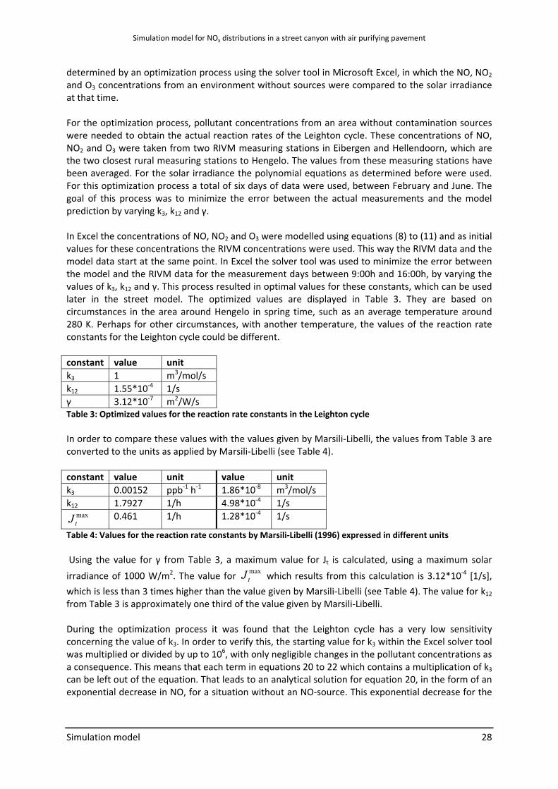
5 Reactor model In order to research the kinetic properties of the air purifying pavement, experiments are done with a laboratory reactor. A simulation model of this reactor is made with the main goal of validating the kinetic equations in the model by comparing the simulation results with the experimental data. In this chapter first the geometry is described (paragraph 7.1), after which the hydrodynamics and mass balance equations with the appropriate boundary conditions are explained in paragraph 7.2 and 7.3. In paragraph 7.4 the researched variables that influence the degradation process are described and the results of the reactor model are presented in paragraph 7.5. In order to verify the way of modelling the active surface only a simple case is researched; only NO is added to the air at the inlet, and because there is no NO2 present at the inlet and only very small concentrations are formed by the degradation process, the reactions from the Leighton cycle are assumed to be negligible.
5.1 Geometry The reactor is a chamber with a stone with TiO2 with a length of 192 mm (active surface), which is placed under a glass plate which does not block UV irradiance. The reactor setup is based on the ISO 22197‐1 (2007) standard (Ballari et al. 2009a). Between the stone and the glass plate, there is a space of 3 mm in which a laminar air flow is present. This flow contains air and predetermined concentrations of NOx at the inlet, and the effect of the active surface is determined by measuring the NOx concentrations at the outlet. In order to model a fully developed laminar flow over the active surface, the length of the reactor model is increased at the inlet to cope with inlet phenomena. The geometry of the reactor model is displayed in , which is a scaled picture.
Figure 17: Geometry of the reactor model with boundary numbers
5.2 Hydrodynamics In order to describe the flow through the reactor, the incompressible Navier‐Stokes equation for a steady state is used, as described in chapter 4. The following values for the variables are taken to calculate the Reynolds number for the flow through the reactor: ρ = 1.207 kg/m3 ; the density of air at a temperature of 10°C and a pressure of 1 atm. u0 = 0.19157 m/s ; the mean inlet velocity L = 0.003 m ; the height of the reactor η = 1.81*10‐5 Pa*s ; the viscosity of air at a temperature of 20°C and a pressure of 1 atm. This results in a Reynolds number of 38 (see equation 1), which represents a laminar flow. Therefore no turbulence terms need to be added to the Navier‐Stokes equation, and equation (4) can be used. In order to establish the laminar flow, and solve the NOx‐distributions within the reactor, appropriate boundary conditions and initial values are needed. Boundary 1 (see ) is defined as an inlet with a condition of a constant normal inflow velocity. Boundary 6 is an outlet with the condition of an equal pressure to the outside of the reactor. All other boundaries are defined as walls without slip, which means that the flow velocity at the wall is equal to zero. The equations that represent these boundary conditions are displayed in Table 5.

Simulation model for NOx distributions in a street canyon with air purifying pavement
Reactor model 32
# Type Boundary conditions 1 Inlet nu ⋅= 0u
2 Wall 0=u 3 Wall 0=u 4 Wall 0=u 5 Wall 0=u 6 Outlet 0))(( =∇+∇ nuu Tη , 0pp =
Table 5: Boundary conditions for the Navier‐Stokes equation for the reactor In Table 5, n is the unit vector perpendicular to the surface 0u is the mean inlet velocity [m/s]
Besides the boundary conditions for the geometry boundaries, the following initial conditions are set for the complete geometry as a starting point for Comsol to determine the steady state solution: Variable Initial value x‐velocity 0 m/s y‐velocity 0 m/s Relative pressure 0 Pa Turbulent kinetic energy 1 m2/s2 Turbulent dissipation rate 1 m2/s3
Table 6: Initial conditions for the complete geometry of the reactor
5.3 Mass balance In order to describe the NOx‐distributions within the reactor the mass balance equations 9a and 9b, as discussed in paragraph 4.3.1, are used. For the active surface of the air purifying pavement, the kinetic equations 10 and 11 from paragraph 4.3.2 are used. Note that the irradiance (E) in equations 10 and 11 represents the UV irradiance in the reactor model. These differential equations are solved by using the appropriate boundary conditions and initial values. At boundary 1 (see ) the (inlet) concentrations of NO and NO2 are constant. The condition for boundary 6 (outlet) is a convective flux, which means that the local NO and NO2 concentrations are controlled by convection. The active surface of the stone (boundary 4) has the boundary condition of a flux over the surface, which represents the heterogeneous reaction rate. The other boundaries are described with an Insulation/Symmetry boundary condition, which means that NOx cannot flow past these boundaries. The equations that represent these boundary conditions are displayed in Table 7. # Type Boundary condition 1 Inlet
inletcc =
2 Wall 0=⋅Nn 3 Wall 0=⋅Nn 4 Active surface
NONO r=⋅Nn , 22 NONO r=⋅Nn
5 Wall 0=⋅Nn 6 Outlet 0)( =∇⋅ cDn Table 7: Boundary conditions for the mass balance equations for the reactor

Simulation model for NOx distributions in a street canyon with air purifying pavement
Reactor model 33
In Table 7, n is the unit vector perpendicular to the surface and N is the flux over the surface. To describe the reaction rate at the active surface of the air purifying stone, the kinetic equations (10 and 11) from paragraph 4.3.2 are used. Besides the boundary conditions for the geometry boundaries, the following initial condition is set for the complete geometry of the reactor, as a starting point for Comsol to determine the steady state solution:
inletcc = for both NO and NO2.
5.4 Variables Most of the reactor experiments have been conducted under similar circumstances, which will be called standard settings from now on. The values for all variables in these standard settings are also used in the simulation model, and are displayed in Table 8. variable description value unit ρ Density of air (T=283 K) 1.207 kg/m3
η Viscosity of air (T=283 K) 1.810*10‐5 kg/m/s D Diffusion coefficient 1.50*10‐5 m2/s k1 Reaction rate constant NO 7.333*10‐8 mol/m2/s k2 Reaction rate constant NO2 2.550*10‐6 mol/m2/s KNO Adsorption equilibrium constant NO 7.610*104 m3/mol KNO2 Adsorption equilibrium constant NO2 3.570*104 m3/mol Cinlet,NO Inlet NO concentration 4.113*10‐5 mol/m3 Cinlet,NO2 Inlet NO2 concentration 0 mol/m3 E UV irradiance 10 W/m2 α Kinetic parameter 2.76 m2/W RH Relative humidity 50 % Kw Adsorption equilibrium constant water 62 m3/mol u0 Inlet velocity 0.1919 m/s Table 8: Standard values for all variables in the reactor The influence of several variables on the NO and NO2 concentrations at the outlet of the reactor has been determined by varying the value of the variable concerned, while keeping all other variables constant at the values displayed in Table 8. The following variables have been researched in this manner:
‐ UV irradiance (range: 0.1 – 26 W/m2) ‐ Inlet NO concentration (range: 4*10‐9 – 4*10‐4 mol/m3) ‐ Relative humidity (range: 40 – 90%) ‐ inlet velocity (range: 0.01 – 5 m/s)
The influence of changes of these variables was researched directly by changing the value of these variables, except for the relative humidity, which needed some additional calculations. In order to calculate the water concentration (cw) as given in the kinetic equations (10) and (11), the concentration of water (kg/m3) for a given relative humidity at a standard temperature and pressure is divided by the molar mass of water. For a relative humidity of 50%, the water content is 0.48 mol/m3. The results of the simulations with the reactor model are presented in the next paragraph.
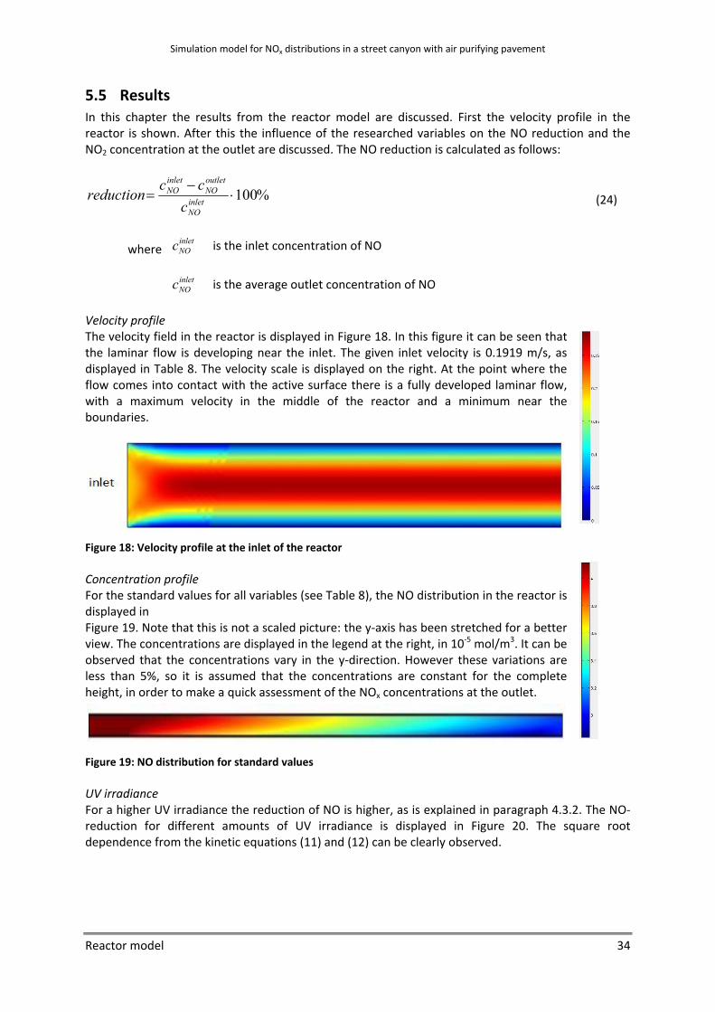
Simulation model for NOx distributions in a street canyon with air purifying pavement
Reactor model 34
5.5 Results In this chapter the results from the reactor model are discussed. First the velocity profile in the reactor is shown. After this the influence of the researched variables on the NO reduction and the NO2 concentration at the outlet are discussed. The NO reduction is calculated as follows:
%100⋅−
= inletNO
outletNO
inletNO
ccc
reduction (24)
where inletNOc is the inlet concentration of NO
inletNOc is the average outlet concentration of NO
Velocity profile The velocity field in the reactor is displayed in Figure 18. In this figure it can be seen that the laminar flow is developing near the inlet. The given inlet velocity is 0.1919 m/s, as displayed in Table 8. The velocity scale is displayed on the right. At the point where the flow comes into contact with the active surface there is a fully developed laminar flow, with a maximum velocity in the middle of the reactor and a minimum near the boundaries.
Figure 18: Velocity profile at the inlet of the reactor Concentration profile For the standard values for all variables (see Table 8), the NO distribution in the reactor is displayed in Figure 19. Note that this is not a scaled picture: the y‐axis has been stretched for a better view. The concentrations are displayed in the legend at the right, in 10‐5 mol/m3. It can be observed that the concentrations vary in the y‐direction. However these variations are less than 5%, so it is assumed that the concentrations are constant for the complete height, in order to make a quick assessment of the NOx concentrations at the outlet.
Figure 19: NO distribution for standard values UV irradiance For a higher UV irradiance the reduction of NO is higher, as is explained in paragraph 4.3.2. The NO‐reduction for different amounts of UV irradiance is displayed in Figure 20. The square root dependence from the kinetic equations (11) and (12) can be clearly observed.
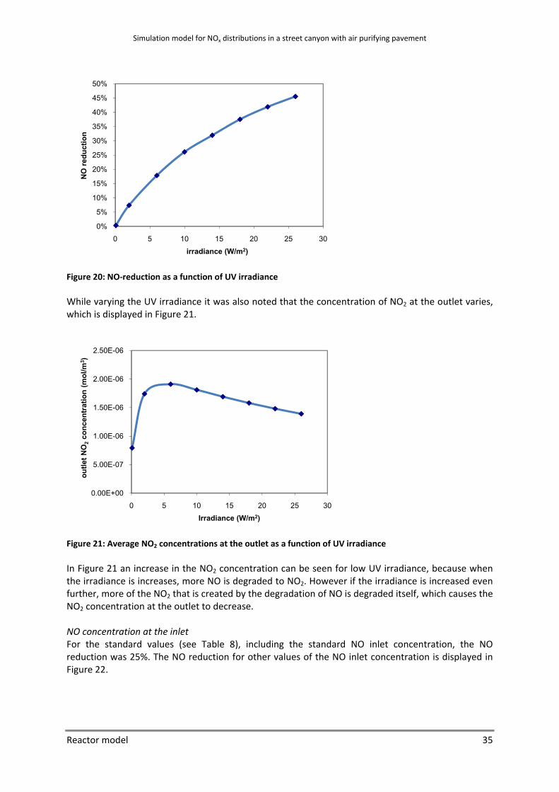
Simulation model for NOx distributions in a street canyon with air purifying pavement
Reactor model 35
Figure 20: NO‐reduction as a function of UV irradiance While varying the UV irradiance it was also noted that the concentration of NO2 at the outlet varies, which is displayed in Figure 21.
Figure 21: Average NO2 concentrations at the outlet as a function of UV irradiance In Figure 21 an increase in the NO2 concentration can be seen for low UV irradiance, because when the irradiance is increases, more NO is degraded to NO2. However if the irradiance is increased even further, more of the NO2 that is created by the degradation of NO is degraded itself, which causes the NO2 concentration at the outlet to decrease. NO concentration at the inlet For the standard values (see Table 8), including the standard NO inlet concentration, the NO reduction was 25%. The NO reduction for other values of the NO inlet concentration is displayed in Figure 22.
0%
5%
10%
15%
20%
25%
30%
35%
40%
45%
50%
0 5 10 15 20 25 30
NO
redu
ctio
n
irradiance (W/m2)
0.00E+00
5.00E-07
1.00E-06
1.50E-06
2.00E-06
2.50E-06
0 5 10 15 20 25 30
outle
t NO
2co
ncen
trat
ion
(mol
/m3 )
Irradiance (W/m2)
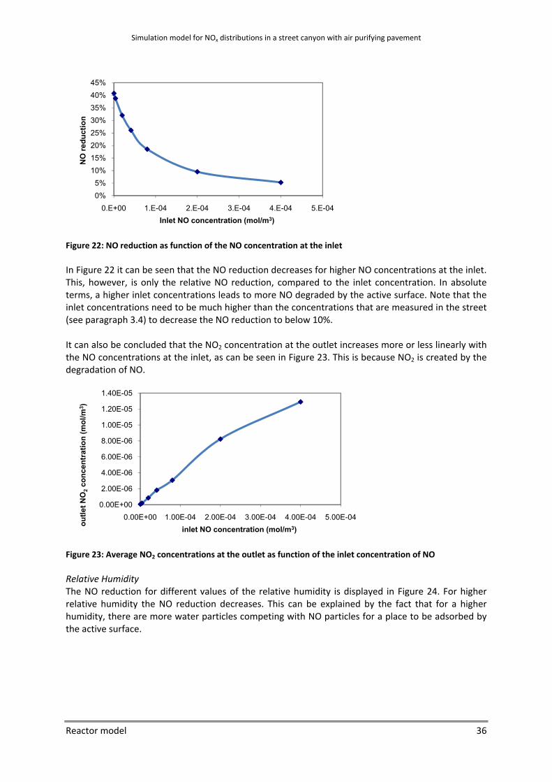
Simulation model for NOx distributions in a street canyon with air purifying pavement
Reactor model 36
Figure 22: NO reduction as function of the NO concentration at the inlet In Figure 22 it can be seen that the NO reduction decreases for higher NO concentrations at the inlet. This, however, is only the relative NO reduction, compared to the inlet concentration. In absolute terms, a higher inlet concentrations leads to more NO degraded by the active surface. Note that the inlet concentrations need to be much higher than the concentrations that are measured in the street (see paragraph 3.4) to decrease the NO reduction to below 10%. It can also be concluded that the NO2 concentration at the outlet increases more or less linearly with the NO concentrations at the inlet, as can be seen in Figure 23. This is because NO2 is created by the degradation of NO.
Figure 23: Average NO2 concentrations at the outlet as function of the inlet concentration of NO Relative Humidity The NO reduction for different values of the relative humidity is displayed in Figure 24. For higher relative humidity the NO reduction decreases. This can be explained by the fact that for a higher humidity, there are more water particles competing with NO particles for a place to be adsorbed by the active surface.
0%5%
10%15%20%25%30%35%40%45%
0.E+00 1.E-04 2.E-04 3.E-04 4.E-04 5.E-04
NO
redu
ctio
n
Inlet NO concentration (mol/m3)
0.00E+00
2.00E-06
4.00E-06
6.00E-06
8.00E-06
1.00E-05
1.20E-05
1.40E-05
0.00E+00 1.00E-04 2.00E-04 3.00E-04 4.00E-04 5.00E-04
outle
t NO
2co
ncen
trat
ion
(mol
/m3 )
inlet NO concentration (mol/m3)

Simulation model for NOx distributions in a street canyon with air purifying pavement
Reactor model 37
Figure 24: NO reduction as function of the relative humidity The NO2 concentrations at the outlet for different values for the relative humidity are displayed in Figure 25. For a higher humidity, the NO2 concentration at the outlet increases. This could be caused by the competition between water and NO2 particles for places on the active surface.
Figure 25: Average NO2 concentration at the outlet as function of the relative humidity Flow rate For an inlet velocity of 0.19 m/s, the flow rate is 3 l/min. The first observation that is made while testing different flow rates is that, for a very high flow rate, the NOx concentrations are distributed differently through the height of the reactor channel as in the case of lower flow rates. For these high flow rates the effects of the active surface are not noticeable throughout the complete channel, but only near the active surface. The concentrations far from the active surface are equal to the inlet concentration. In this case the influence of diffusion on the distribution of the pollutants is less important than convection. However the average outlet concentrations are still similar to the outlet concentrations that are calculated based on a plug flow rate. An example of this is displayed in Figure 26, where the image of the reactor has been expanded in vertical direction to show the effect of convection more clearly.
0%
10%
20%
30%
40%
50%
60%
0 20 40 60 80 100
NO
redu
ctio
n
RH (%)
0.00E+00
1.00E-06
2.00E-06
3.00E-06
0 20 40 60 80 100
Out
let N
O2
conc
entr
atio
n (m
ol/m
3 )
RH (%)
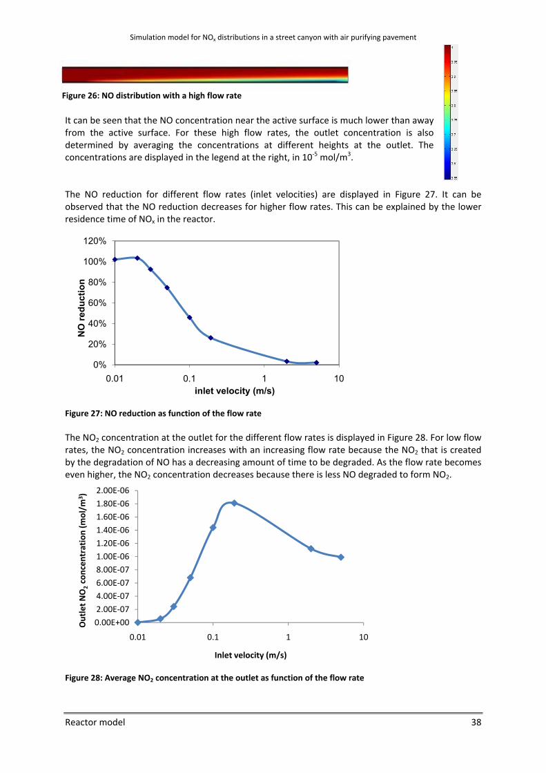
Simulation model for NOx distributions in a street canyon with air purifying pavement
Reactor model 38
It can be seen that the NO concentration near the active surface is much lower than away from the active surface. For these high flow rates, the outlet concentration is also determined by averaging the concentrations at different heights at the outlet. The concentrations are displayed in the legend at the right, in 10‐5 mol/m3. The NO reduction for different flow rates (inlet velocities) are displayed in Figure 27. It can be observed that the NO reduction decreases for higher flow rates. This can be explained by the lower residence time of NOx in the reactor.
Figure 27: NO reduction as function of the flow rate The NO2 concentration at the outlet for the different flow rates is displayed in Figure 28. For low flow rates, the NO2 concentration increases with an increasing flow rate because the NO2 that is created by the degradation of NO has a decreasing amount of time to be degraded. As the flow rate becomes even higher, the NO2 concentration decreases because there is less NO degraded to form NO2.
Figure 28: Average NO2 concentration at the outlet as function of the flow rate
0%
20%
40%
60%
80%
100%
120%
0.01 0.1 1 10
NO
redu
ctio
n
inlet velocity (m/s)
0.00E+002.00E‐07
4.00E‐076.00E‐07
8.00E‐071.00E‐06
1.20E‐061.40E‐06
1.60E‐061.80E‐06
2.00E‐06
0.01 0.1 1 10
Outlet N
O2concen
tration (m
ol/m
3 )
Inlet velocity (m/s)
Figure 26: NO distribution with a high flow rate
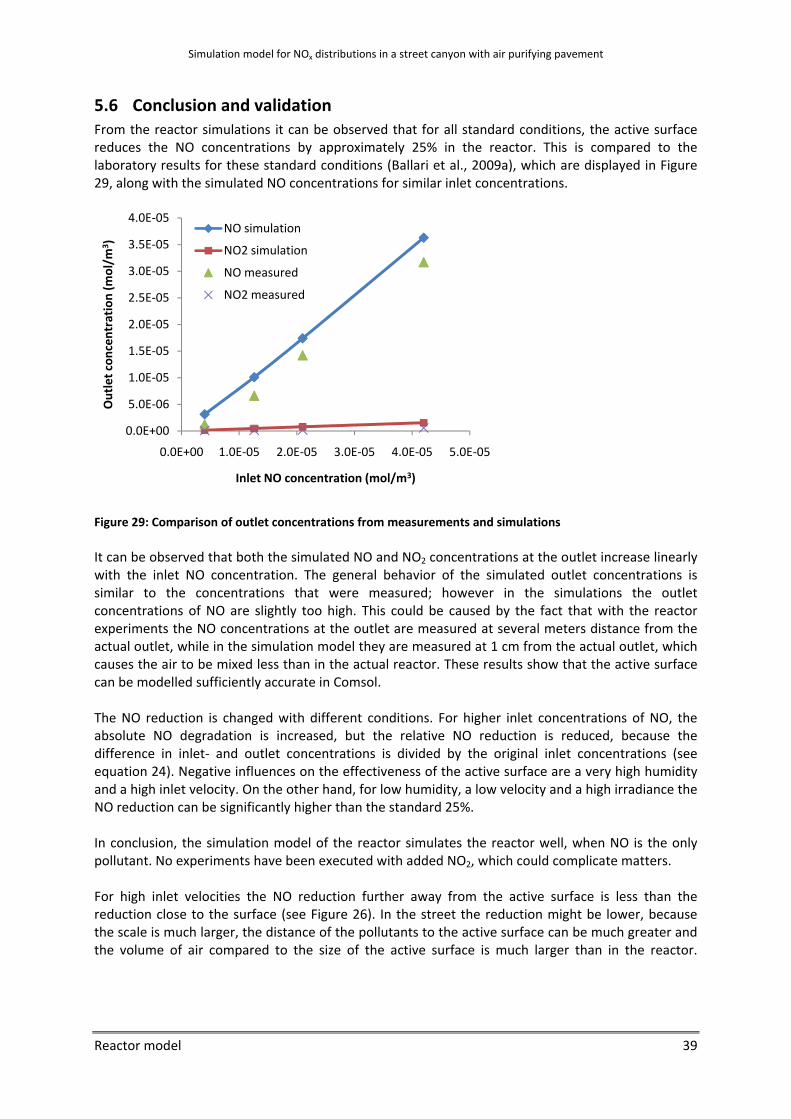
Simulation model for NOx distributions in a street canyon with air purifying pavement
Reactor model 39
5.6 Conclusion and validation From the reactor simulations it can be observed that for all standard conditions, the active surface reduces the NO concentrations by approximately 25% in the reactor. This is compared to the laboratory results for these standard conditions (Ballari et al., 2009a), which are displayed in Figure 29, along with the simulated NO concentrations for similar inlet concentrations.
Figure 29: Comparison of outlet concentrations from measurements and simulations It can be observed that both the simulated NO and NO2 concentrations at the outlet increase linearly with the inlet NO concentration. The general behavior of the simulated outlet concentrations is similar to the concentrations that were measured; however in the simulations the outlet concentrations of NO are slightly too high. This could be caused by the fact that with the reactor experiments the NO concentrations at the outlet are measured at several meters distance from the actual outlet, while in the simulation model they are measured at 1 cm from the actual outlet, which causes the air to be mixed less than in the actual reactor. These results show that the active surface can be modelled sufficiently accurate in Comsol. The NO reduction is changed with different conditions. For higher inlet concentrations of NO, the absolute NO degradation is increased, but the relative NO reduction is reduced, because the difference in inlet‐ and outlet concentrations is divided by the original inlet concentrations (see equation 24). Negative influences on the effectiveness of the active surface are a very high humidity and a high inlet velocity. On the other hand, for low humidity, a low velocity and a high irradiance the NO reduction can be significantly higher than the standard 25%. In conclusion, the simulation model of the reactor simulates the reactor well, when NO is the only pollutant. No experiments have been executed with added NO2, which could complicate matters. For high inlet velocities the NO reduction further away from the active surface is less than the reduction close to the surface (see Figure 26). In the street the reduction might be lower, because the scale is much larger, the distance of the pollutants to the active surface can be much greater and the volume of air compared to the size of the active surface is much larger than in the reactor.
0.0E+00
5.0E‐06
1.0E‐05
1.5E‐05
2.0E‐05
2.5E‐05
3.0E‐05
3.5E‐05
4.0E‐05
0.0E+00 1.0E‐05 2.0E‐05 3.0E‐05 4.0E‐05 5.0E‐05
Outlet con
centration
(mol/m
3 )
Inlet NO concentration (mol/m3)
NO simulation
NO2 simulation
NO measured
NO2 measured

Simulation model for NOx distributions in a street canyon with air purifying pavement
40
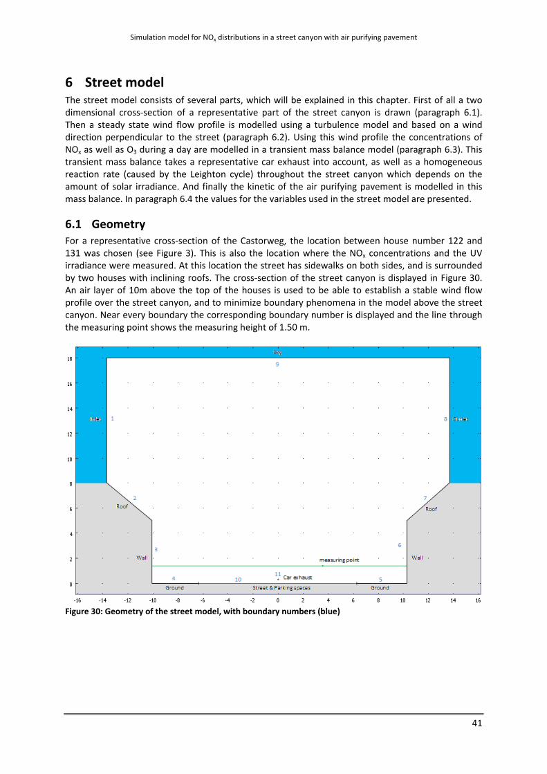
Simulation model for NOx distributions in a street canyon with air purifying pavement
41
6 Street model The street model consists of several parts, which will be explained in this chapter. First of all a two dimensional cross‐section of a representative part of the street canyon is drawn (paragraph 6.1). Then a steady state wind flow profile is modelled using a turbulence model and based on a wind direction perpendicular to the street (paragraph 6.2). Using this wind profile the concentrations of NOx as well as O3 during a day are modelled in a transient mass balance model (paragraph 6.3). This transient mass balance takes a representative car exhaust into account, as well as a homogeneous reaction rate (caused by the Leighton cycle) throughout the street canyon which depends on the amount of solar irradiance. And finally the kinetic of the air purifying pavement is modelled in this mass balance. In paragraph 6.4 the values for the variables used in the street model are presented.
6.1 Geometry For a representative cross‐section of the Castorweg, the location between house number 122 and 131 was chosen (see Figure 3). This is also the location where the NOx concentrations and the UV irradiance were measured. At this location the street has sidewalks on both sides, and is surrounded by two houses with inclining roofs. The cross‐section of the street canyon is displayed in Figure 30. An air layer of 10m above the top of the houses is used to be able to establish a stable wind flow profile over the street canyon, and to minimize boundary phenomena in the model above the street canyon. Near every boundary the corresponding boundary number is displayed and the line through the measuring point shows the measuring height of 1.50 m.
Figure 30: Geometry of the street model, with boundary numbers (blue)
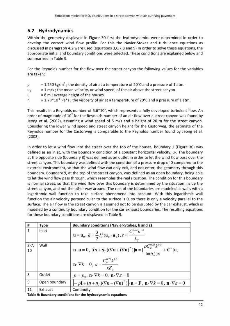
Simulation model for NOx distributions in a street canyon with air purifying pavement
42
6.2 Hydrodynamics Within the geometry displayed in Figure 30 first the hydrodynamics were determined in order to develop the correct wind flow profile. For this the Navier‐Stokes and turbulence equations as discussed in paragraph 4.2 were used (equations 3,6,7,8 and 9) In order to solve these equations, the appropriate initial and boundary conditions were selected. These conditions are explained below and summarized in Table 9. For the Reynolds number for the flow over the street canyon the following values for the variables are taken: ρ = 1.250 kg/m3 ; the density of air at a temperature of 20°C and a pressure of 1 atm. u0 = 1 m/s ; the mean velocity, or wind speed, of the air above the street canyon L = 8 m ; average height of the houses η = 1.78*10‐5 Pa*s ; the viscosity of air at a temperature of 20°C and a pressure of 1 atm. This results in a Reynolds number of 5.6*105, which represents a fully developed turbulent flow. An order of magnitude of 107 for the Reynolds number of an air flow over a street canyon was found by Jeong et al. (2002), assuming a wind speed of 5 m/s and a height of 20 m for the street canyon. Considering the lower wind speed and street canyon height for the Castorweg, the estimate of the Reynolds number for the Castorweg is comparable to the Reynolds number found by Jeong et al. (2002). In order to let a wind flow into the street over the top of the houses, boundary 1 (Figure 30) was defined as an inlet, with the boundary condition of a constant horizontal velocity, u0. The boundary at the opposite side (boundary 8) was defined as an outlet in order to let the wind flow pass over the street canyon. This boundary was defined with the condition of a pressure drop of 0 compared to the external environment, so that the wind flow can only exit, and not enter, the geometry through this boundary. Boundary 9, at the top of the street canyon, was defined as an open boundary, being able to let the wind flow pass through, which resembles the real situation. The condition for this boundary is normal stress, so that the wind flow over this boundary is determined by the situation inside the street canyon, and not the other way around. The rest of the boundaries are modeled as walls with a logarithmic wall function to take surface phenomena into account. With this logarithmic wall function the air velocity perpendicular to the surface is 0, so there is only a velocity parallel to the surface. The air flow in the street canyon is assumed not to be disrupted by the car exhaust, which is modeled by a continuity boundary condition for the car exhaust boundaries. The resulting equations for these boundary conditions are displayed in Table 9. # Type Boundary conditions (Navier‐Stokes, k and ε) 1 Inlet
0uu = , )(23
002 uu ⋅= TIk ,
TLkC 5.175.0
με =
2‐7, 10
Wall 0=⋅un , unuu ]
)ln([)])()([(
5.025.0+
+ +=∇+∇+ CkC
w
TT κδ
ρηη μ
,
0=∇⋅ kn , w
kCκδ
ε μ5.175.0
=
8 Outlet 0pp = , 0=∇⋅ kn , 0=∇⋅ εn
9 Open boundary [ ] FnuuI =⋅∇+∇++− ))()(( TTp ηη , 0=∇⋅ kn , 0=∇⋅ εn
11 Exhaust Continuity Table 9: Boundary conditions for the hydrodynamic equations

Simulation model for NOx distributions in a street canyon with air purifying pavement
43
In Table 9, n is the unit vector perpendicular to the surface 0u is the mean inlet velocity [m/s]
TI is the turbulence intensity, and has a value of 0.05
TL is the turbulence length, and has a value of 0.01 m
wδ is the wall offset, which is set to half the height of the local mesh element
κ is the von Kármán constant, and has a value of 0.42 +C is a universal constant for smooth walls, and has a default value of 5.5
and w
ww
kCκδ
ρδδ μ
5.025.0
=+
Besides the boundary conditions for the geometry boundaries, the following initial conditions are needed for the complete geometry for Comsol to determine the steady state solution: Variable Initial value x‐velocity 0 m/s y‐velocity 0 m/s Relative pressure 0 Pa Turbulent kinetic energy 1 m2/s2 Turbulent dissipation rate 1 m2/s3
Table 10: Initial conditions for the complete geometry of the street canyon These initial conditions ensure that the wind flow in the street canyon is only determined by the wind that enters the system at the inlet, and is not disrupted by anything within the street canyon.
6.3 Mass balance For the mass balance in the street canyon a transient model is used, because the traffic density, the irradiance and both the homogeneous and heterogeneous reaction rates are not constant throughout a day. The general mass balance equations (9a), (9b) and (9c) as discussed in paragraph 4.3 are used to describe the transport of the pollutants. For the active surface of the air purifying pavement, the kinetic equations (10) and (11) from paragraph 4.3.2 are used. Note that the irradiance (E) in equations (10) and (11) represents the total solar irradiance in the street model. For the homogeneous reaction rate throughout the street canyon equations (20), (21) and (22), representing the Leighton cycle, are used. In order to solve these equations, the appropriate boundary conditions need to be selected. These boundary conditions are discussed below and summarize in Table 11 after which the details for the car exhaust, the background concentration and the active surface are explained. At boundaries 1 and 9 (see Figure 30) the concentration is set to a value that is equal to the background concentration. Boundary 8 is modeled with a “convective flux” boundary condition, which means that the local NOx and O3 concentrations are controlled by convection. The walls and ground without active surface receive an “Insulation/Symmetry” boundary condition, meaning that pollutants cannot flow past these boundaries. The active surface is modeled with the boundary condition of a flux that is described with kinetic equations 10 and 11 for NO and NO2 respectively. In case of a normal street surface, this flux is set to 0. The car exhaust is modeled by a circle with a radius of 3 cm within the street canyon, at a height of 30 cm. Across the perimeter boundary a flux

Simulation model for NOx distributions in a street canyon with air purifying pavement
44
(J), normal to this boundary, of NO and NO2 was set as a boundary condition, to simulate the gases emitted by a car exhaust The equations describing these boundary conditions are given in Table 11. # Type Boundary condition 1 Inlet backgroundcc =
2‐7 Wall 0=⋅Nn 8 Outlet 0)( =∇⋅ cDn
9 Sky backgroundcc =
10 Normal surface 0=⋅ NONn , 02=⋅ NONn
Active surface NONO r=⋅Nn ,
22 NONO r=⋅Nn
11 Exhaust exhaustNNNn =⋅⋅ )( 21
Table 11: Boundary conditions for the mass balance equations In Table 11, n is the unit vector perpendicular to the surface
N is the flux over the surface N1, N2 respectively represent the total flux outside and inside the car exhaust
boundary. Besides the boundary conditions for the geometry boundaries, the following initial condition is needed for the street canyon:
0cc = for NO, NO2 and O3
Where 0c is the concentration in the street at 9:00h [mol/m3]
Background concentration The initial background concentrations are set to the values that were measured at 9:00h on the measurement day that is simulated. This way the starting conditions for the measurement day and the model are equal. However the background concentrations do not stay constant during the day, because they are changed as a result of the Leighton cycle. This fact needs to be taken into account for an accurate model and therefore the background concentrations are formulated as follows:
tRcc backgroundbackground ⋅+= 0
(25)
Where 0backgroundc is the background concentration at 9:00h [mol/m3]
R is the homogeneous reaction rate, described in equations (20), (21) and (22) [mol/m3/s]
t is the time in seconds, starting with 0 at 9:00h [s] Air purifying pavement In order to determine the influence of the air purifying pavement in different circumstances, these circumstances need to be modeled both with a normal and an air purifying street surface. In case of an active surface (e.g. with air purifying pavement) the boundary condition of a flux over the surface, as displayed in Table 11 is needed. For a normal street surface, the boundary condition is changed to “Insulation/Symmetry”, just like any other wall.
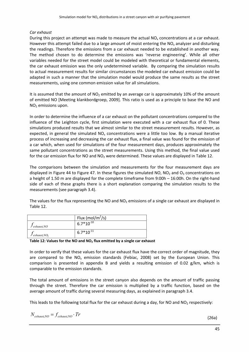
Simulation model for NOx distributions in a street canyon with air purifying pavement
45
Car exhaust During this project an attempt was made to measure the actual NOx concentrations at a car exhaust. However this attempt failed due to a large amount of moist entering the NOx analyzer and disturbing the readings. Therefore the emissions from a car exhaust needed to be established in another way. The method chosen to do determine the emissions was ‘reverse engineering’. While all other variables needed for the street model could be modeled with theoretical or fundamental elements, the car exhaust emission was the only undetermined variable. By comparing the simulation results to actual measurement results for similar circumstances the modeled car exhaust emission could be adapted in such a manner that the simulation model would produce the same results as the street measurements, using one common emission value for all simulations. It is assumed that the amount of NO2 emitted by an average car is approximately 10% of the amount of emitted NO [Meeting klankbordgroep, 2009]. This ratio is used as a principle to base the NO and NO2 emissions upon. In order to determine the influence of a car exhaust on the pollutant concentrations compared to the influence of the Leighton cycle, first simulation were executed with a car exhaust flux of 0. These simulations produced results that we almost similar to the street measurement results. However, as expected, in general the simulated NOx concentrations were a little too low. By a manual iterative process of increasing and decreasing the car exhaust flux, a final value was found for the emission of a car which, when used for simulations of the four measurement days, produces approximately the same pollutant concentrations as the street measurements. Using this method, the final value used for the car emission flux for NO and NO2 were determined. These values are displayed in Table 12. The comparisons between the simulation and measurements for the four measurement days are displayed in Figure 44 to Figure 47. In these figures the simulated NO, NO2 and O3 concentrations on a height of 1.50 m are displayed for the complete timeframe from 9:00h – 16:00h. On the right‐hand side of each of these graphs there is a short explanation comparing the simulation results to the measurements (see paragraph 3.4). The values for the flux representing the NO and NO2 emissions of a single car exhaust are displayed in Table 12. Flux (mol/m2/s)
NOexhaustf , 6.7*10‐10
2,NOexhaustf 6.7*10‐11
Table 12: Values for the NO and NO2 flux emitted by a single car exhaust In order to verify that these values for the car exhaust flux have the correct order of magnitude, they are compared to the NOx emission standards (Febiac, 2008) set by the European Union. This comparison is presented in appendix B and yields a resulting emission of 0.02 g/km, which is comparable to the emission standards. The total amount of emissions in the street canyon also depends on the amount of traffic passing through the street. Therefore the car emission is multiplied by a traffic function, based on the average amount of traffic during several measuring days, as explained in paragraph 3.4. This leads to the following total flux for the car exhaust during a day, for NO and NO2 respectively:
TrfN NOexhaustNOexhaust ⋅= ,, (26a)
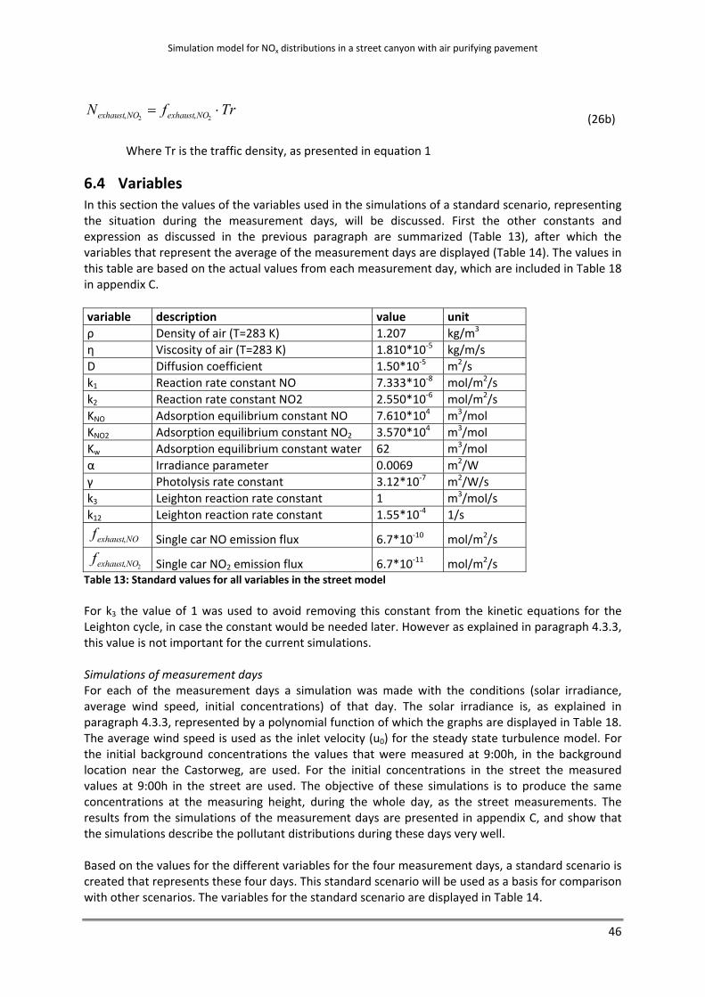
Simulation model for NOx distributions in a street canyon with air purifying pavement
46
TrfN NOexhaustNOexhaust ⋅=22 ,, (26b)
Where Tr is the traffic density, as presented in equation 1
6.4 Variables In this section the values of the variables used in the simulations of a standard scenario, representing the situation during the measurement days, will be discussed. First the other constants and expression as discussed in the previous paragraph are summarized (Table 13), after which the variables that represent the average of the measurement days are displayed (Table 14). The values in this table are based on the actual values from each measurement day, which are included in Table 18 in appendix C. variable description value unit ρ Density of air (T=283 K) 1.207 kg/m3
η Viscosity of air (T=283 K) 1.810*10‐5 kg/m/s D Diffusion coefficient 1.50*10‐5 m2/s k1 Reaction rate constant NO 7.333*10‐8 mol/m2/s k2 Reaction rate constant NO2 2.550*10‐6 mol/m2/s KNO Adsorption equilibrium constant NO 7.610*104 m3/mol KNO2 Adsorption equilibrium constant NO2 3.570*104 m3/mol Kw Adsorption equilibrium constant water 62 m3/mol α Irradiance parameter 0.0069 m2/W γ Photolysis rate constant 3.12*10‐7 m2/W/s k3 Leighton reaction rate constant 1 m3/mol/s k12 Leighton reaction rate constant 1.55*10‐4 1/s
NOexhaustf , Single car NO emission flux 6.7*10‐10 mol/m2/s
2,NOexhaustf Single car NO2 emission flux 6.7*10‐11 mol/m2/s Table 13: Standard values for all variables in the street model For k3 the value of 1 was used to avoid removing this constant from the kinetic equations for the Leighton cycle, in case the constant would be needed later. However as explained in paragraph 4.3.3, this value is not important for the current simulations. Simulations of measurement days For each of the measurement days a simulation was made with the conditions (solar irradiance, average wind speed, initial concentrations) of that day. The solar irradiance is, as explained in paragraph 4.3.3, represented by a polynomial function of which the graphs are displayed in Table 18. The average wind speed is used as the inlet velocity (u0) for the steady state turbulence model. For the initial background concentrations the values that were measured at 9:00h, in the background location near the Castorweg, are used. For the initial concentrations in the street the measured values at 9:00h in the street are used. The objective of these simulations is to produce the same concentrations at the measuring height, during the whole day, as the street measurements. The results from the simulations of the measurement days are presented in appendix C, and show that the simulations describe the pollutant distributions during these days very well. Based on the values for the different variables for the four measurement days, a standard scenario is created that represents these four days. This standard scenario will be used as a basis for comparison with other scenarios. The variables for the standard scenario are displayed in Table 14.
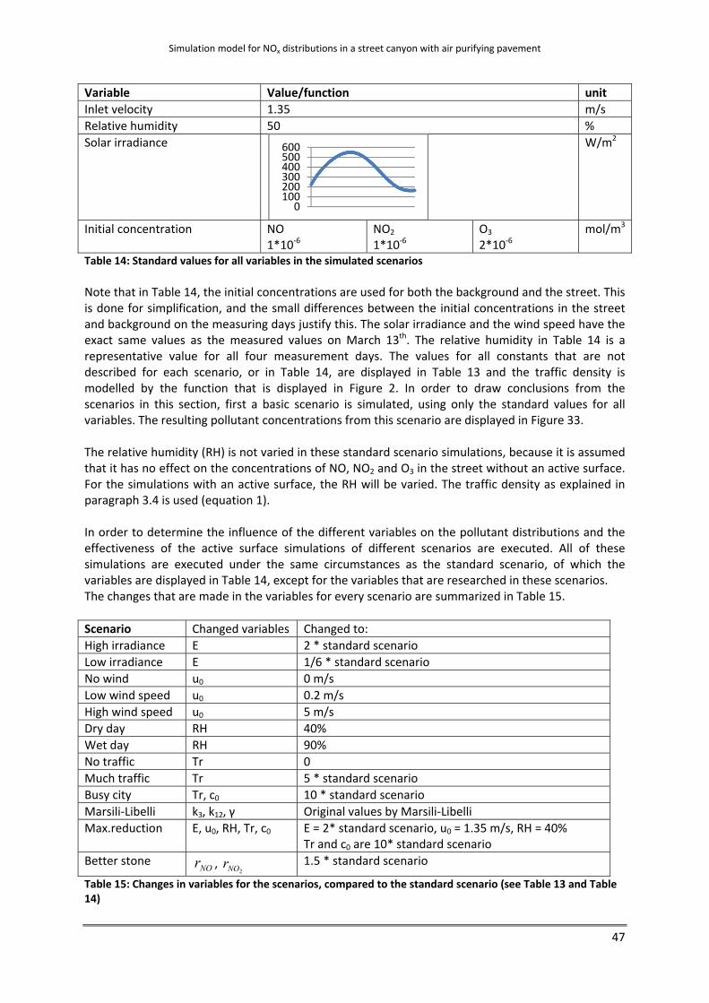
Simulation model for NOx distributions in a street canyon with air purifying pavement
47
Variable Value/function unit Inlet velocity 1.35 m/s Relative humidity 50 % Solar irradiance W/m2
Initial concentration NO 1*10‐6
NO2 1*10‐6
O3 2*10‐6
mol/m3
Table 14: Standard values for all variables in the simulated scenarios Note that in Table 14, the initial concentrations are used for both the background and the street. This is done for simplification, and the small differences between the initial concentrations in the street and background on the measuring days justify this. The solar irradiance and the wind speed have the exact same values as the measured values on March 13th. The relative humidity in Table 14 is a representative value for all four measurement days. The values for all constants that are not described for each scenario, or in Table 14, are displayed in Table 13 and the traffic density is modelled by the function that is displayed in Figure 2. In order to draw conclusions from the scenarios in this section, first a basic scenario is simulated, using only the standard values for all variables. The resulting pollutant concentrations from this scenario are displayed in Figure 33. The relative humidity (RH) is not varied in these standard scenario simulations, because it is assumed that it has no effect on the concentrations of NO, NO2 and O3 in the street without an active surface. For the simulations with an active surface, the RH will be varied. The traffic density as explained in paragraph 3.4 is used (equation 1). In order to determine the influence of the different variables on the pollutant distributions and the effectiveness of the active surface simulations of different scenarios are executed. All of these simulations are executed under the same circumstances as the standard scenario, of which the variables are displayed in Table 14, except for the variables that are researched in these scenarios. The changes that are made in the variables for every scenario are summarized in Table 15. Scenario Changed variables Changed to: High irradiance E 2 * standard scenario Low irradiance E 1/6 * standard scenario No wind u0 0 m/s Low wind speed u0 0.2 m/s High wind speed u0 5 m/s Dry day RH 40% Wet day RH 90% No traffic Tr 0 Much traffic Tr 5 * standard scenario Busy city Tr, c0 10 * standard scenario Marsili‐Libelli k3, k12, γ Original values by Marsili‐Libelli Max.reduction E, u0, RH, Tr, c0 E = 2* standard scenario, u0 = 1.35 m/s, RH = 40%
Tr and c0 are 10* standard scenario Better stone
NOr , 2NOr 1.5 * standard scenario
Table 15: Changes in variables for the scenarios, compared to the standard scenario (see Table 13 and Table 14)
0100200300400500600

Simulation model for NOx distributions in a street canyon with air purifying pavement
48
In chapter 7 the results from the standard scenario and the other scenarios, of which the variables are presented in Table 15, including the effectiveness of the active surface are presented. The results from the simulations of the measurement days are presented in appendix C.

Simulation model for NOx distributions in a street canyon with air purifying pavement
Street model results 49
7 Street model results In this chapter the results from the simulations with the street model will be discussed. First the results from the simulations are discussed in paragraph 7.1. These results will be the basis for the validation of the street model. In paragraph 0 some other scenarios and their results are discussed. Based on these results the effectiveness of the air purifying pavement will be discussed in paragraph 7.3 by comparing the results from similar simulations with and without an active surface.
7.1 Results from simulations of measurement days For every simulation, the velocity field of the wind throughout the street canyon has the same shape, independent of the inlet velocity (see Figure 31). The magnitude of the velocity at any point in the geometry does depend on the inlet velocity.
Figure 31: Velocity profile of the wind in the street model The direction of the arrows in Figure 31 indicates the wind direction, and the magnitude of the arrows indicates the wind speed in that direction. The largest arrows (e.g. the highest wind speed) are above the street canyon and represent a wind speed which is equal to the inlet velocity. It can be seen that between the houses a circulating flow is developed, with much lower wind speeds than above the street canyon. This circulating flow has already been acknowledged in other research by Jeong et al. (2002) and Sallizoni et al. (2007). The wind speed between the houses increases linearly with the inlet velocity. This circulating velocity field results in a circulating flow for the pollutants, with a consequential asymmetric pollutant distribution over the street canyon. An example of this asymmetric distribution is displayed in Figure 32, which shows the NO2 concentration throughout the street canyon at 13:00h for a standard scenario that is based on the measurement days. The variables for this standard scenario are discussed in the next paragraph.

Simulation model for NOx distributions in a street canyon with air purifying pavement
Street model results 50
Figure 32: Simulated NO2 distribution at 13:00h for a standard scenario, without active surface In Figure 32 it can be observed that the NO2 concentration at the measuring point (see Figure 30) is much different than the concentrations at a height of 1.50m in other locations in the street. This is the case for the bulk of the simulations, and therefore the conclusion has been drawn that the concentrations at this measuring point are not representative for the complete street in the simulation model. Consequently, the pollutant concentrations throughout the complete width of the street canyon at a height of 1.50 m are observed for the street simulations (see green line in Figure 30). In order to present the pollutant concentrations at these locations in a clear way, the distribution along this line is plotted for every hour. It can also be observed from Figure 32, in which the NO2 distribution is representative for all street simulations, that the area between the houses can roughly be separated into two areas. One of these areas is on the left‐hand side of the street, where the emissions from the car exhaust play an important role because they are transported into this area directly by the wind flow. The other area is on the right‐hand side of the street. In this area the car exhaust emissions play an insignificant role, compared to the Leighton cycle. Especially in the green part from Figure 32 the wind speed is low, and the emissions from the car exhaust are hardly transported into this area. Instead these emissions are circulated around this area. In general this leads to relatively low NOx levels and relatively high O3 levels in this area. The pollutant concentrations for the simulations of the measurement days are displayed in Appendix C (Figure 44 to Figure 47).

Simulation model for NOx distributions in a street canyon with air purifying pavement
Street model results 51
7.2 Results from other scenarios The scenarios that are described in this chapter are based on a standard set of values for all variables, except the variables that are explicitly described for each scenario. These standard settings are displayed in Table 14. In these graphs, one line for each hour represents the pollutant concentrations at that moment during the day, ranging from 9:00h until 16:00h:
The concentrations at these times are displayed for a height in the street canyon of 1.50 m. On the x‐axis of each graph in Figure 33, the distance from the center of the street (x=0) is displayed in m. The line colors and distances on the x‐axis as explained above are used in all following graphs in this chapter. They are also used for all graphs in Appendix C and D.
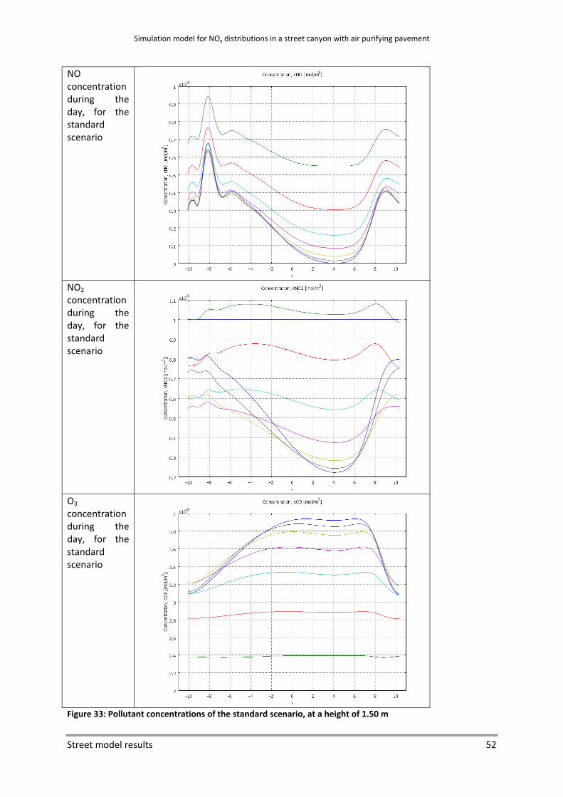
Street m
NO concentrduring day, fostandardscenario
NO2 concentrduring day, fostandardscenario
O3 concentrduring day, fostandardscenario
Figure 33
Simul
model results
ration the
or the d o
ration the
or the d o
ration the
or the d o
3: Pollutant co
ation model fo
oncentrations
or NOx distributi
s of the stand
ions in a street
ard scenario,
canyon with ai
at a height o
ir purifying pav
f 1.50 m
ement
52

Simulation model for NOx distributions in a street canyon with air purifying pavement
Street model results 53
A continuous decrease in NO concentrations can be observed in Figure 33. The NO2 concentration initially increases slightly, which can be contributed to the low irradiance in the morning. After this short increase, the NO2 concentrations continuously decrease. The O3 concentrations increase during the whole day. Note that the variations in the concentrations are larger at the right‐hand side of the street. The NOx concentrations on that side are below average, while the O3 concentrations are above the average value. The effects of other scenarios can thus be determined by reviewing the differences with the standard scenario. For this comparison only the concentrations at a height of 1.50m will be used, as was done for the standard scenario. In this paragraph only the most important conclusions for each scenario, without active surface, will be discussed. Each scenario is simulated for a normal street and for a street with an active surface of air purifying pavement. The effectiveness of the active surface can then be determined by reviewing the differences between these simulations. The conclusions from the simulations of a normal street are listed in this paragraph. Note that no simulation has been executed for different values for the relative humidity in a normal street, because it is assumed that this variable has no influence in this case. The comparison between the simulations of a normal street and with an active surface is done in paragraph 7.3. The graphs from all scenarios are included in appendix D. The changes and influences of the different variables on the pollutant distributions in the street are listed below. High irradiance The four measurement days were all in February and March. The irradiance will be significantly higher in summer, and therefore a simulation is run with an amount of irradiance that is representative for a summer day. The function for the solar irradiance is set to the double of the standard irradiance function, so that the peak irradiance is just above 1000 W/m2, which means that the peak UV irradiance is just above 25 W/m2. In this scenario the NO concentrations are exactly the same as in the standard scenario (see Figure 51). This can be explained by the fact that the irradiance in the Leighton cycle does not influence the NO concentrations. The NO2 concentrations are approximately 50% lower, while the O3 concentrations are approximately 10% higher. This is the result of the photolysis process from the Leighton cycle. Low irradiance A maximum solar irradiance of 90 W/m2 can be measured on a foggy, dark day, which is approximately one sixth of the maximum irradiance on March 13th. Therefore the irradiance function for this foggy day is set to one sixth of the standard irradiance. In this scenario the NO concentrations are exactly the same as in the standard scenario (see Figure 52). The NO2 concentration however increases strongly during the first half of the day, after which the average concentration stabilizes during the second half. The increase can be contributed to the lower irradiance, which causes less NO2 to be degraded by photolysis. The O3 concentration continuously increases, which is also the case in the standard scenario. However the increase is less than half as large, which can also be contributed to the low amount of photolysis. No wind For theoretical purposes a simulation was run without wind or, in other words, without convection, leaving diffusion as the only means of mass transport. Note that this is not a realistic scenario, because in reality there is always movement of air when there is traffic.

Simulation model for NOx distributions in a street canyon with air purifying pavement
Street model results 54
In this scenario the pollutant concentrations are the highest at the location of the car exhaust, decreasing circularly with the distance from this point (see Figure 53). Because there is no convection, the pollutants are not spread as much as in the standard scenario, and the maximum NOx levels are significantly higher at the car exhaust location. The concentrations in the rest of the street are significantly lower. Low wind speed A simulation was executed with a very low wind speed of 0.2 m/s, which is almost 7 times lower than the wind speed for the standard scenario. In this scenario the pollutant is transported very slowly by the wind, which results in concentrations at the left‐hand side of the street that are up to 3 times as high as in the standard scenario (see Figure 54). On the right hand side of the street, the area with very low NOx concentrations is larger compared to the standard scenario. High wind speed On the four measurement days the wind speed was relatively low. Therefore an extra simulation is run with a significantly higher wind speed of 5 m/s, which is almost 4 times the standard wind speed. The variation in both the NO and NO2 concentrations for different locations in the street canyon is much less with a high wind speed (see Figure 55). This can be contributed to the fact that the pollution is mixed better with this high wind speed. Both the NO and NO2 concentrations are also approximately 5% lower than in the standard scenario, and the O3 concentration is approximately 10% lower. This is because the higher wind speed transports more pollutants away from the street canyon. Dry day / wet day No simulations were executed for a dry or wet day with a normal street surface, because it is assumed that the relative humidity does not influence the pollutant distributions in this case. Instead for these simulations with a normal street surface the results of the standard scenario are used (see Figure 56 and Figure 57). No traffic A simulation without traffic was run to determine the concentrations in a relatively unpolluted area. The NO concentrations on the right‐hand side of the street are similar to the NO concentrations in the standard scenario (see Figure 58). However the concentrations on the left‐hand side are between 20 and 60% lower than in the standard scenario. This can be contributed to the wind at a height of 1.50m, which flows from the right‐hand side to the left‐hand side of the street. Normally the wind would transport the pollution from the car exhaust in the middle of the street towards the left‐hand side of the street first, but in this case there are no emissions to be transported. The NO2 concentrations are approximately 10% lower than in the standard scenario and the O3 concentrations are less than 5% lower than in the standard scenario. The most important reason for these reductions being relatively low, compared to the reduction in traffic density, is that the Leighton cycle degrades much more NO2 than the amount that is emitted by traffic. Therefore, for a relatively quiet street like the Castorweg, the influence of the Leighton cycle is much stronger than the influence of the traffic density. Much traffic In order to determine the pollutant concentrations of a very busy street a simulation is run with five times the normal traffic intensity.
Simulation model for NOx distributions in a street canyon with air purifying pavement
Street model results 55
While in the standard scenario the NO concentration continuously decreases and the NO2 concentration decreases after a slight initial increase, the behaviour in this scenario is very different (see Figure 59). Instead of a decreasing, both the NO and the NO2 concentrations increase at the left‐hand side of the street. This can be explained by the higher traffic density, which is now more significant compared to the Leighton cycle. On the right‐hand side of the street the NOx concentrations still decrease due to the Leighton cycle. However at locations with a relatively higher wind speed the NOx concentrations are higher, because they are transported there by the wind flow. The O3 concentrations are up to 15% higher with the increased traffic density. Busy city Because the Castorweg is a relatively quiet street, an extra simulation is executed to represent a busy city. For this simulation the initial concentrations and the traffic density have been multiplied by 10. The NOx concentrations in this simulation are 10 times the concentrations of the standard scenario, which is according to expectations (see Figure 60). The O3 concentrations however is approximately 5% lower than the tenfold of the standard scenario. This can be attributed to the fact that the Leighton cycle is less significant for this relatively high traffic density. Marsili‐Libelli In order to determine the effect of the optimization process for the reaction rate constants in the Leighton cycle, a simulation is executed with the original value for these constants (see Table 4), as used by Marsili‐Libelli (1996). The simulated NO concentrations during the day are significantly lower than the standard scenario and the NO2 concentrations show an increase instead of a decrease as in the standard scenario (see Figure 61). The O3 concentrations are higher than in the standard scenario. The increase in NO2 can be explained by the lower value for γ which causes less NO2 to be degraded by photolysis. The relatively low NO concentrations can be attributed to the high value for k12 in this simulation. This causes more NO to be degraded into NO2, according to equation (18). The increased O3 concentration can be explained by the lack of available NO for the reaction in equation (15). From this simulation it can be concluded that the original value for the reaction rate constants for the Leighton cycle, as used by Marsili‐Libelli, are less representative for a standard day in the Castorweg. Maximum reduction In order to determine the maximum potential pollutant reduction by the air purifying pavement, a simulation is executed with most variables set to the values from the previous scenarios that are most favourable for the effectiveness of the active surface (see Table 15). The results from this scenario are presented in the next paragraph. Better stone In order to determine the potential effect of a better air purifying stone, a simulation has been executed with 1.5 times the reaction rates for NO and NO2 at the active surface, compared to the standard scenario. The results from this scenario and the effectiveness of the active surface in the other scenarios are presented in the next paragraph.
7.3 Effectiveness air purifying pavement In this paragraph the results from all scenarios with and without active surface are compared, to determine the effectiveness of the air purifying pavement in reducing the NO and NO2 levels in the street canyon at a height of 1.50m. In Figure 34 the NO2 distribution throughout the street canyon

Simulation model for NOx distributions in a street canyon with air purifying pavement
Street model results 56
for the standard scenario, with air purifying pavement, at 13:00h are displayed. The NO2 scale of this figure is similar to the scale in Figure 32, which displays the NO2 distribution for the same situation without air purifying pavement, and thus the effect of the active surface can be observed by reviewing the colour differences. At very low distances from the active surface (5cm), the NO reduction can reach 25% and the NO2 reduction can reach up to 90%. However, this decreases with the height for the main part of the street. This behaviour for different heights can also be observed in Figure 48 to Figure 50 in appendix D. Especially on the left‐hand side of the street the reduction is relatively high, because the circulating wind profile transports the pollutants over a larger part of the active surface, causing the residence time of the air above the active surface to be longer in that region.
Figure 34: Simulated NO2 distribution at 13:00h for a standard scenario, with active surface In order to present the results for the different scenarios at other times during each day, the concentrations at each hour of the day, at a height of 1.50 m will be displayed. This is done in the same way as in Figure 33, as is explained in paragraph 0. The concentrations from the standard scenario with and without active surface are displayed in Figure 35. The effectiveness of the active surface in other scenarios is then compared to this scenario. The graphs from the simulations with an active surface are presented in appendix D. Note that the legends on the right‐hand side of the graphs in Figure 35 give the appropriate time in seconds. This corresponds with the lines as described in paragraph 0, with 9:00h represented by the time of 0 seconds. In Figure 35 it can be observed that the NO concentration with the active surface is mostly similar to the NO concentration in a normal street. However, at locations with a relatively high NO concentration, these concentrations are reduced by a maximum of 2%. In other words: the maximum NO reduction is 2%. The NO2 reduction is approximately 10% at the locations in the street where the NO2 concentration is the largest. O3 levels are reduced by approximately 2%.

Street m
The concscale on
Figure 3for an ac
Simul
model results
centrations dthe y‐axis fo
5: Concentratctive street su
ation model fo
displayed in or a quicker c
tions of NO (turface (right),
or NOx distributi
Figure 35 arecomparison
top), NO2 (mid, in the standa
ions in a street
e also displaof the differe
ddle) and O3 (ard scenario,
canyon with ai
yed Figure 4ent scenario
(bottom) for aat a height of
ir purifying pav
48 in appendos.
a normal stref 1.50 m
ement
ix D, using a
eet surface (le
57
nother
eft) and

Simulation model for NOx distributions in a street canyon with air purifying pavement
Street model results 58
The effect of the air purifying pavement can also be determined on a more global scale, by reviewing the average reduction throughout the width of the street for the total area under 1.50 m. These average reductions are displayed in Figure 36. It can be observed that the global reduction during the day for NO in this area reaches a maximum of 6% and the NO2 reduction is reaches 19%. The O3 levels are reduced by a maximum of approximately 2%. These maximum reductions are reached during the time of the day that the irradiance is at its maximum. Comparing these global reductions to the maximum reductions at a height of 1.50 m, it can be concluded that the global reductions are significantly better. It should be considered however, that the global reductions up to higher altitudes would be lower, because the effect of the air purifying pavement diminishes with longer distances. In the remainder of this project only the reductions at a height of 1.50 m will be compared, because this is the only measuring height in the protocol (Ballari et al., 2008) that represents the breathing height.
Figure 36: Average concentrations in the standard scenario for the total area under 1.50 m

Simulation model for NOx distributions in a street canyon with air purifying pavement
Street model results 59
The maximum reductions at 1.50m by the air purifying pavement for all scenarios are listed in Table 16. These maximum reductions are valid for the locations in the street where the pollutant concentrations are the highest. In locations with lower concentrations, the reductions can be smaller. Actually the reduction for most simulations is the highest in the corner of the house and the sidewalk on the left‐hand side of the street, because the wind speed is almost 0 there. For a fair estimate this maximum is not taken into account. This maximum reduction was usually observed during a period of time around noon, when the irradiance is relatively high. For most scenarios this period of time is almost as long as the whole day, which means that the maximum reduction listed in Table 16 is present during the main part of the day. Scenario NO reduction (%) NO2 reduction (%) O3 reduction (%) Figure number Standard 2 10 2 Figure 48 High irradiance 2 10 2 Figure 51 Low irradiance <1 10 1 Figure 52 No wind 6 18 16 Figure 53 Low wind speed 2 10 4 Figure 54 High wind speed 1 10 1 Figure 55 Dry day 2 13 2 Figure 56 Wet day <1 8 <1 Figure 57 No traffic 2 10 <1 Figure 58 Much traffic 2 10 2 Figure 59 Busy city 3 12 3 Figure 60 Marsili‐Libelli 2 15 2 Figure 61 Max. reduction 3 17 3 Figure 62 Better stone 2 12 2 Figure 63 Table 16: Effectiveness of the active surface for different scenarios (see Table 15) In the right‐hand side column of Table 16, the figure number refers to the figure in appendix D, where the results for the corresponding scenario are displayed. The street simulations show that for a street like the Castorweg, under normal circumstances the effect of the air purifying pavement on the pollutant concentrations at a height of 1.50m is threefold. The NO and O3 levels can be reduced by 2%, while the reduction of NO2 levels can reach 10%. At lower heights the effect of the active surface is considerably larger, as can be observed in Figure 34. These reduction rates can be influenced by changes in the irradiance, wind speed, relative humidity and traffic density. In general, the effectiveness of the air purifying pavement increases for a higher irradiance, because more electron‐holes can be formed at the active surface. For a very high irradiance the effectiveness of the active surface is increased only slightly for a significant increase in irradiance, as was the case for the high irradiance scenario. This can also be observed in the kinetic equations (11) and (12) for the active surface. A lower wind speed can also be beneficial for the effectiveness of the air purifying pavement, because the residence time of the pollutants near the active surface is higher. However a low wind speed can also cause less dispersion of the emissions, causing less pollutant particles to reach the active surface. Another positive influence on the effectiveness of the air purifying pavement is a low humidity. As can be observed in kinetic equations 10 and 11, the higher the water content, the lower the

Simulation model for NOx distributions in a street canyon with air purifying pavement
Street model results 60
degradation rate, because the pollutants are competing with water particles for sites at the active surface. Finally, for higher concentrations and more sources of NOx the effectiveness of the air purifying pavement is increased, because more sites at the active surface are occupied by pollutant particles. For the simulations with the original Marsili‐libelli constants, a higher NO2 reduction is found compared to the standard scenario. This can be explained by the fact that less NO2 is degraded by photolysis, causing more NO2 to be adsorbed by the active surface. For the simulations with a better stone, of which the NO and NO2 reduction are 1.5 times higher than in the standard scenario, a higher NO2 reduction was found, as was expected. However due to convection and diffusion in the street, the factor of 1.5 was not found at a height of 1.50 m. The NO2 reduction at this height was only 1.2 times the reduction of the standard scenario, which can be attributed to pollutant transport by convection and diffusion. Combining the most favourable circumstances for the effectiveness of the air purifying pavement, the NO and O3 reduction can be increased to 3% and the NO2 reduction can reach 17%. These reductions are significantly higher than for the standard scenario.
7.4 Discussion During this project many assumptions have been made and many different sources and methods of data gathering have been used. Therefore the accomplished results have to be interpreted in the right way to use them correctly. In this chapter the validity of the results is discussed to help interpret them. Comparison between simulation model and measurement results In order to validate the simulation model of the street, the concentrations that are determined by the simulations of the four measurement days (without active surface) are compared to the concentrations that have actually been measured during those days. This is done by comparing the simulation average concentrations for every whole hour at a height of 1.50m to the measurement results at the same times. This method contains two sources for inaccuracies; first of all, the measuring location in the street might not be representative for the rest of the street, and secondly the instantaneous concentrations might not be representative for the average concentrations during that hour. Other errors could lie in the fact that only four measurement days were used for this comparison, which might not be representative for other days or circumstances. Effectiveness of the air purifying pavement Most of the variables were validated by the comparison between the simulation and the measurements described above, however since it was impossible to measure in the Castorweg after the application of air purifying pavement, the effect of the air purifying pavement could not be validated by the street measurements. The modelling of the active surface however was done on a basis of chemical fundamentals, and proved to predict accurate results for the reactor model under specific circumstances. This provides validation for the modelling of the active surface. Furthermore, for the amount of traffic that passes through the Castorweg, it is concluded that the influence of the Leighton cycle in decreasing the NOx concentrations is much more important than the influence of the traffic in increasing these concentrations. Therefore the Castorweg, with the current traffic density, is not an ideal street to determine the maximum capacity of the air purifying pavement.
Simulation model for NOx distributions in a street canyon with air purifying pavement
Street model results 61
Assumptions in the modelling of the UV irradiance For the UV irradiance in Comsol three assumptions were made. First of all the solar irradiance in Comsol is modelled using a polynomial fit that describes the irradiance that was actually measured. This polynomial function represents the solar irradiance well on a global scale, but details such as short peaks are not included. Secondly it is assumed that the UV irradiance always has the same ration compared to the total solar irradiance, which might be slightly inaccurate. And finally, it is assumed that the irradiance is equal throughout the complete street canyon, so for example shadow or reflection was not taken into account. These assumptions can produce inaccuracies in both the optimization process for the Leighton cycle constants and in the simulations results. Assumptions in the modelling of the car emission The car emission is the only variable in this report which was not based on a theoretical background or measurements. Because all other variables used in the street model for a normal surface could be directly measured or determined by appropriate theories, this car emission was the only remaining unknown. Therefore the emission was determined by an iterative process that had the objective of establishing one common value for the car emission for which the street simulations would produce similar results compared to the results from the measurement days. For this optimization the assumption was made that the amount of NO2 emitted by a vehicle was 10% of the NO emission. Also instead of modelling separate vehicles, a function is used to model the average traffic density during a day. The results from the simulations should therefore be interpreted on a global scale, meaning that only the general behaviour is predicted by the model and not, for example, the detailed impact of one passing vehicle. A comparison of the car emission used in this project to the European emission standard (see Appendix B) indicates that the values for the project have a realistic order of magnitude. Assumptions in the modelling of the wind flow profile The wind flow profile within the street canyon was not validated by measurements, because of difficult circumstances during the measurement days. However the fact that a similar circulating patterns exists in street canyons was already acknowledged in other literature (Jeong et al., 2002 and Salizzoni et al., 2007). In reality the passing of traffic most likely causes turbulence which disturbs the flow profile, however in the simulation model this fact has been neglected in order to avoid unnecessary complexity. Because of the wind flow profile, the simulated NOx distributions are not symmetrical for the street canyon. This has not been validated by simultaneous measurements at both sides of the street. Assumptions for RIVM data For the optimization of the Leighton constants RIVM data from two rural measuring stations were used to represent relatively unpolluted environments. For the modelling of the Leighton cycle it was assumed that these measuring stations were not at all influenced by any NOx sources. However in reality this could be inaccurate, causing the Leighton constants to be inaccurate as well. Inaccuracies in the Comsol model Within Comsol the concentrations as well as the reaction rates for the Leighton cycle are recalculated for every simulated minute. More accurate results could have been reached with a smaller step size; however the duration of each simulation would have increased significantly for only a slightly more accurate result. Another inaccuracy from the Comsol model lies in the use of streamline diffusion to solve the mass balance. This is a method used to simplify convection‐diffusion modeling, which assumes that most

Simulation model for NOx distributions in a street canyon with air purifying pavement
Street model results 62
of the diffusion is along the convection direction. This streamline diffusion could be an exaggeration of the reality; however it was not possible to solve the mass balance without it. Comparison with other practical experiments A NOx reduction of approximately 30% was measured by Guerrini et al. (2007) in Bergamo (Italy), which is significantly more than the NOx reduction predicted by the simulation model. The reduction of 30% however was measured at a height of 30 cm. At greater distances from the air purifying pavement NOx reductions were determined to be lower (20% at 1.80 m height). This is however still more reduction than predicted by the simulation model. There are several factors which can contribute to this difference. First of all, the buildings around the measurement street from Guerrini et al. (2007) were much higher than the houses in the Castorweg and the wind speed was negligible during those measurements. This causes pollutants to have a longer residence time in the street, which allows the air purifying pavement to degrade more NOx. Secondly, the irradiance and temperature are likely to be higher in Italy, even though the measurements by Guerrini et al. (2007) were also executed in winter. A higher temperature could decrease the amount of NO2 that is caught by organic pollutants, with higher NO concentrations as a consequence. Finally the traffic density in the measurement street in Bergamo was most likely higher than in the Castorweg, since the street in Bergamo is a main urban connection route while the Castorweg is a side street.
Simulation model for NOx distributions in a street canyon with air purifying pavement
Conclusions and recommendations 63
8 Conclusions and recommendations In this chapter the conclusions from this project are presented, after which several recommendations are made concerning future use and improvement of the simulation model.
8.1 Conclusions In paragraph 2.3, the research questions for this project are formulated. The answers to these questions are presented in this chapter, after which these conclusions are discussed in the next chapter. First the influence of the researched variables on the general behaviour of pollutants in the street canyon is presented, after which the effectiveness of the active surface is described. Wind speed The wind speed has a relatively small influence on the pollutant levels in the street, within the range that is common for the Castorweg. When the wind direction is perpendicular to the street, a circulating flow is established, which transports car emission through the street. The NOx levels are distributed more equally throughout the street canyon when the wind speed is high, because the air is mixed more. NOx levels are also slightly lower for a high wind speed because pollutants are transported out of the street canyon faster. Traffic Passing traffic can significantly increase the instantaneous NOx levels; however the average NOx and O3 levels are only slightly increased. An increasing traffic density results in higher pollutant levels at the side of the street where the wind directly transports the pollutants. However the influence of the traffic density on the pollutant levels at the other side of the street is only marginal. Relative humidity The relative humidity is assumed to have no influence on the pollutant levels in a normal street. It does have a significant influence on the effectiveness of the active surface. Compared to a normal day, a higher humidity can decrease the NO2 reduction by the active surface significantly while a lower humidity can significantly increase this reduction. NOx concentrations For areas with much higher pollutant concentrations compared to the Castorweg, the relative changes in the pollutant concentrations during a day are similar to the Castorweg. The effectiveness of the active surface however is increased. Atmospheric reactions and UV irradiance Atmospheric reactions in the form of the Leighton cycle have a dominant effect on the NOx and O3 levels in the Castorweg. Under the influence of UV irradiance NO2 photolysis takes place, which starts a cycle that creates and degrades NO, NO2 and O3. In general the NOx levels are decreased by this process, while the O3 levels increase during the day. The amount of organic pollutants available as well as the temperature could alter the effect of the Leighton cycle. With lower levels of organic pollutants or higher temperatures, the NO levels could be higher than predicted by the simulation model. Effectiveness of air purifying pavement For an average day in the Castorweg, the simulation model predicts a NO reduction at a height of 1.50 m of 2% and a NO2 reduction of 10% by the air purifying pavement. The O3 levels are also reduced by 2%. Considering not only the pollutant levels at 1.50m height, but the complete area under this height, the NO reduction is 6%, the NO2 reaches 19% and the O3 reduction is still approximately 2%.

Simulation model for NOx distributions in a street canyon with air purifying pavement
Conclusions and recommendations 64
Because the effectiveness of the air purifying pavement is dependent on the UV irradiance, just as the Leighton cycle, most of its potential NOx reduction is already established by the Leighton cycle. Therefore the effectiveness of the active surface is lower than the initial expectations. However at a height of 1.50m especially the NO2 reduction by the active surface is still significant with 10% in the Castorweg. The NOx reduction in the Castorweg could prove to be higher than the predictions by the simulation model if there are few organic pollutants or if the temperature is higher so less NO2 is removed from the atmosphere.
8.2 Recommendations In order to completely validate the simulation model, two parts of future research are required:
‐ First, the NO and NO2 emissions of vehicles that pass through the Castorweg should
be directly measured to validate or adapt the values used in this report. ‐ Secondly, measurements need to be executed in the Castorweg after the application
of the air purifying pavement to validate the effect of the active surface.
More extensive research is also useful in the following areas:
‐ Laboratory experiments should be executed with both NO and NO2 at the inlet, and it would be useful to measure the O3 concentrations as well, to determine the effect of the Leighton cycle.
‐ Laboratory experiments could be executed with a bigger air flow channel, to measure the effects of the active surface when a larger part of the pollutants does not pass through the direct vicinity of the active surface.
‐ Laboratory experiments could be executed to determine the long term effectiveness of air purifying stones, with and without periodically washing the stone.
‐ A simplified kinetic model was used in this project to describe the reactions in the Leighton cycle. In order to better understand the influence of this cycle on pollutant concentrations and of different atmospheric conditions on the Leighton cycle more laboratory experiments could be done without an active surface.
‐ A 3‐dimensional simulation model of the street could provide more insight in the effect of wind from other directions, or turbulence caused by vehicles, on the pollutant levels or the effectiveness of the air purifying pavement in the street.
‐ Street measurements should be executed with air purifying pavement in much more polluted areas, such as busy roads in large cities.
‐ The degradation of organic pollutants by the air purifying pavement could be researched along with the influence of organic pollutants on the Leighton cycle.
Simulation model for NOx distributions in a street canyon with air purifying pavement
References 65
References Ballari M.M., Brouwers, H.J.H., (2008) Air quality monitoring protocol in Castorweg for the demonstration air purifying pavement project in Hengelo city, Department of Construction Management & Engineering, Faculty of Engineering Technology, University of Twente, Enschede, The Netherlands Ballari M.M., Hunger M., Hüsken G. and Brouwers H.J.H., (2009a) Heterogeneous Photocatalysis Applied to Concrete Pavement for Air Remediation, 3rd International Symposium on Nanotechnology in Construction NICOM3,31st May‐ 2nd June, Prague, Czech Republic Ballari M.M., Hunger M., Hüsken G. and Brouwers H.J.H., (2009b) NOx photocatalytic degradation employing concrete pavement with titanium dioxide. A kinetic study, submission in progress Beeldens A., (2007) Air Purification by road materials: results of the test project in Antwerp, International RILEM Symposium on Photocatalysis, Environment and Construction Materials 8‐9 October 2007, Florence, Italy Bohn B., Rohrer F., Brauers T. and Wahner A., (2005) Actinometric measurements of NO2 photolysis frequencies in the atmosphere simulation chamber SAPHIR, Atmospheric Chemistry and Physics, 5, 493‐503 Cassar L., Beeldens A., Pimpinelli N. and Guerrini G.L., (2007) Photocatalysis of cementitious materials, International RILEM Symposium on Photocatalysis, Environment and Construction Materials 8‐9 October 2007, Florence, Italy Council of the European Union, (1999) Council Directive 1999/30/EC ‐ relating to limit values for sulphur dioxide, nitrogen dioxide and oxides of nitrogen, particulate matter and lead in ambient air Devahasdin S., Fan C., Li J.K. and Chen D.H., (2003) TiO2 Photocatalytic Oxidation of Nitric Oxide: Transient Behavior and Reaction Kinetics, Journal of Photochemistry and Photobiology A: Chemistry 156: 161‐170 Fowler D. et al., (1998) The atmospheric budget of oxidized nitrogen and its role in ozone formation and deposition, New Phytologist, 139, 11‐23 Ghormley J.A., Ellsworth R.L. and Hochanadel C.J., (1973) Reaction of excited oxygen atoms with nitrous oxide. Rate constants for reaction of ozone with nitric oxide and with nitrogen oxide, The Journal of Physical Chemistry, Volume 77, No. 11 Guerrini G.L. and Peccati E., (2007) Photocatalytic cementitious roads for depollution, International RILEM Symposium on Photocatalysis, Environment and Construction Materials 8‐9 October 2007, Florence, Italy Hunger M. and Brouwers H.J.H., (2008) Self‐Cleaning Surfaces as an innovative potential for sustainable concrete, submission in progress Jeong S.J. and Andrews M.J., (2002) Application of the k–e turbulence model to the high Reynolds number skimming flow field of an urban street canyon, Atmospheric Environment, 36, 1137‐1145
Simulation model for NOx distributions in a street canyon with air purifying pavement
References 66
Kilifarska N.A. and Haigh J.D., (2005) The impact of solar variability on the middle atmosphere in present‐day and pre‐industrial atmospheres, Journal of Atmospheric and Solar‐Terrestrial Physics, 241‐249 Maggos T., Plassais A., Bartzis J.G., Vasilakos C., Moussiopoulos N., Bonafous L., (2008) Photocatalytic Degradation of NOx in a Pilot Street Canyon Configuration Using TiO2‐Mortar Panels, Environmental Monitoring and Assessment, 136, 35‐44 Marsili‐Libelli S., (1996) Simplified kinetics of tropospheric ozone, Ecological Modelling, 84, 233‐244 Meeting Klankbordgroep, 7 January 2009, Enschede, the Netherlands Murata Y., Tawara H., Obata H.O. and Hirosi T., (1999) Air purifying pavement: development of photocatalytic concrete blocks, Journal of Advanced Oxidation Technology 4 (2), 227‐230 Salizzoni P. et al., (2007) Wind Tunnel Study of the Exchange between a Street Canyon and the External Flow, Centre National de la Recherche Scientifique, France Zafonte L., Rieger P.L., Holmes J.R., (2002) Nitrogen dioxide in the Los Angeles atmosphere, Environmental Science & Technology 11 (5), 483‐487 Internet Febiac, 2008, http://www.febiac.be/public/content.aspx?FID=587 RIVM, 2009, http://www.lml.rivm.nl

Simulation model for NOx distributions in a street canyon with air purifying pavement
Nomenclature 67
Nomenclature Re = Reynolds number
ρ = density of the medium [kg/m3]
u0 = mean inlet velocity [m/s]
L = representative length [m]
η = viscosity of the medium [Pa*s]
u = velocity vector [m/s]
p = pressure [Pa]
I = unity vector
η = viscosity of the medium [Pa*s]
Tη = turbulent viscosity [Pa*s]
T)( u∇ = turbulent velocity term, based on the fluctuation of u around its mean value
F = body force vector [N/m3]
k = turbulence energy [m2/s2]
σk = experimentally determined constant: 1.0
ε = dissipation rate of turbulent energy [m2/s3]
σε = experimentally determined constant: 1.3
Cε1 = experimentally determined constant: 1.44
Cε2 = experimentally determined constant: 1.92
Cμ = experimentally determined constant: 0.09
D = diffusion coefficient [m2/s]
NOc = concentration of NO [mol/m3]
2NOc = concentration of NO2 [mol/m3]
NOR = homogeneous reaction rate for NO [mol/m3/s]
2NOR = homogeneous reaction rate for NO2 [mol/m3/s]
3OR = homogeneous reaction rate for O3 [mol/m3/s]
NOr = reaction rate at the active surface for NO [mol/m2/s]
2NOr = reaction rate at the active surface for NO2 [mol/m2/s]
k1 = reaction rate constant for the degradation of NO [mol/m2/s]
k2 = reaction rate constant for the degradation of NO2 [mol/m2/s]
α = irradiance parameter [m2/W]

Simulation model for NOx distributions in a street canyon with air purifying pavement
Nomenclature 68
E = irradiance flux [W/m2]*
KNO = adsorption equilibrium constant for NO [m3/mol]
KNO2 = adsorption equilibrium constant for NO2 [m3/mol]
Kw = adsorption equilibrium constant for water [m3/mol]
Wc = concentration of H2O in the air over the active surface [mol/m3]
tJ = reaction rate constant for the photolysis process [1/s]
k3 = reaction rate constant for the degradation of NO by O3 [m3/mol/s]
k12 = reaction rate constant for the degradation of NO by radicals [1/s]
γ = constant conversion factor for the photolysis process [m2/W/s]

Simulation model for NOx distributions in a street canyon with air purifying pavement
Appendices 69
Appendices Appendix A: Leighton optimization Appendix B: validation of car exhaust flux Appendix C: Simulation results for the measurement days Appendix D: Simulation results for all scenarios

Simulation model for NOx distributions in a street canyon with air purifying pavement
Appendices 70
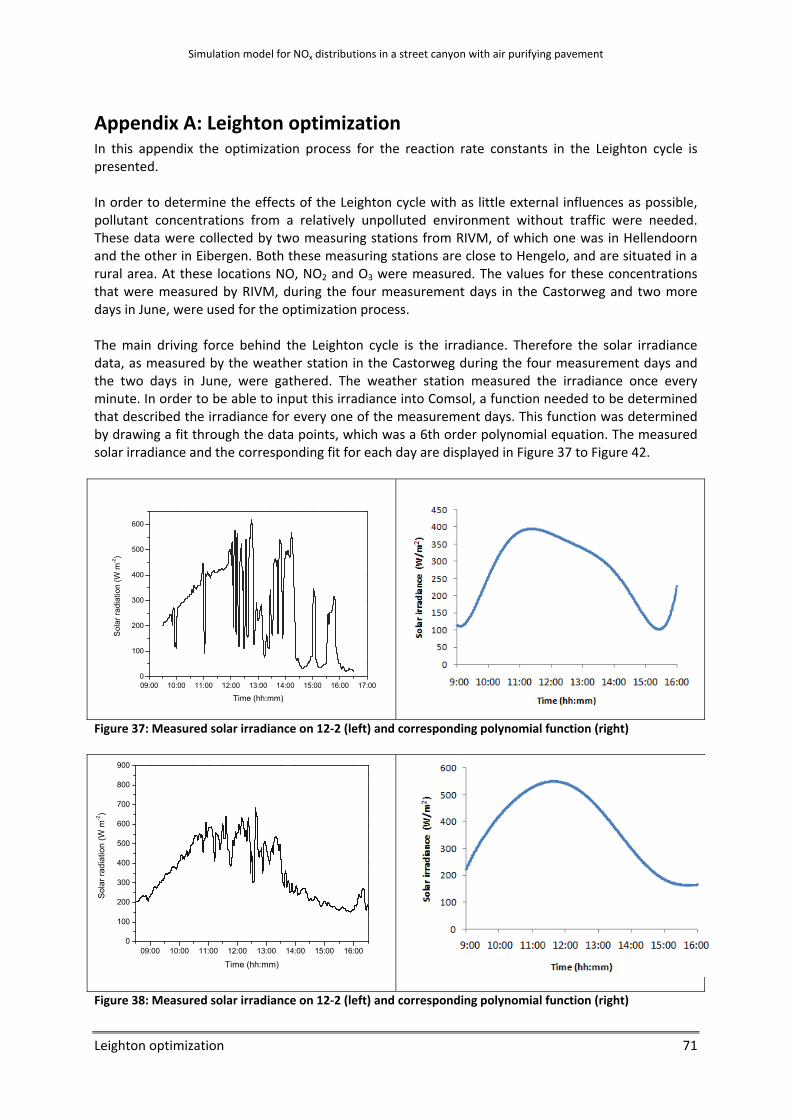
Simulation model for NOx distributions in a street canyon with air purifying pavement
Leighton optimization 71
Appendix A: Leighton optimization In this appendix the optimization process for the reaction rate constants in the Leighton cycle is presented. In order to determine the effects of the Leighton cycle with as little external influences as possible, pollutant concentrations from a relatively unpolluted environment without traffic were needed. These data were collected by two measuring stations from RIVM, of which one was in Hellendoorn and the other in Eibergen. Both these measuring stations are close to Hengelo, and are situated in a rural area. At these locations NO, NO2 and O3 were measured. The values for these concentrations that were measured by RIVM, during the four measurement days in the Castorweg and two more days in June, were used for the optimization process. The main driving force behind the Leighton cycle is the irradiance. Therefore the solar irradiance data, as measured by the weather station in the Castorweg during the four measurement days and the two days in June, were gathered. The weather station measured the irradiance once every minute. In order to be able to input this irradiance into Comsol, a function needed to be determined that described the irradiance for every one of the measurement days. This function was determined by drawing a fit through the data points, which was a 6th order polynomial equation. The measured solar irradiance and the corresponding fit for each day are displayed in Figure 37 to Figure 42.
Figure 37: Measured solar irradiance on 12‐2 (left) and corresponding polynomial function (right)
Figure 38: Measured solar irradiance on 12‐2 (left) and corresponding polynomial function (right)
09:00 10:00 11:00 12:00 13:00 14:00 15:00 16:00 17:000
100
200
300
400
500
600
Sol
ar ra
diat
ion
(W m
-2)
Time (hh:mm)
09:00 10:00 11:00 12:00 13:00 14:00 15:00 16:000
100
200
300
400
500
600
700
800
900
Sol
ar ra
diat
ion
(W m
-2)
Time (hh:mm)
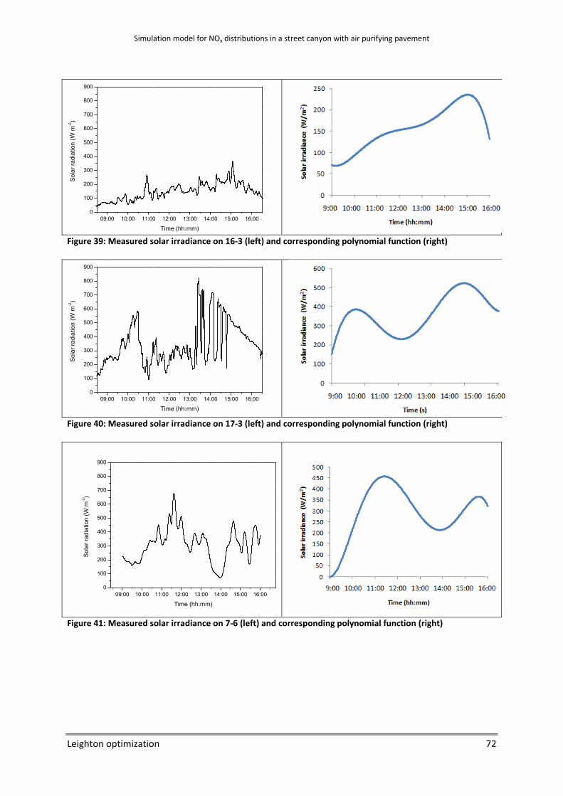
Simulation model for NOx distributions in a street canyon with air purifying pavement
Leighton optimization 72
Figure 39: Measured solar irradiance on 16‐3 (left) and corresponding polynomial function (right)
Figure 40: Measured solar irradiance on 17‐3 (left) and corresponding polynomial function (right)
Figure 41: Measured solar irradiance on 7‐6 (left) and corresponding polynomial function (right)
09:00 10:00 11:00 12:00 13:00 14:00 15:00 16:000
100
200
300
400
500
600
700
800
900
S
olar
radi
atio
n (W
m-2)
Time (hh:mm)
09:00 10:00 11:00 12:00 13:00 14:00 15:00 16:000
100
200
300
400
500
600
700
800
900
Sol
ar ra
diat
ion
(W m
-2)
Time (hh:mm)
09:00 10:00 11:00 12:00 13:00 14:00 15:00 16:000
100
200
300
400
500
600
700
800
900
Sol
ar ra
diat
ion
(W m
-2)
Time (hh:mm)

Simulation model for NOx distributions in a street canyon with air purifying pavement
Leighton optimization 73
Figure 42: Measured solar irradiance on 8‐6 (left) and corresponding polynomial function (right) From these graphs it can be observed that the global behavior of the polynomial fit represents the data well, although the level of detail is low. Using the polynomial fits for the irradiance and the kinetics for the Leighton cycle by Marsili‐Libelli (equations 20, 21 and 22) the pollutant concentrations are calculated for every minute between 9:00h and 16:00 in Excel. The resulting concentrations at each whole hour (9:00h, 10:00h, etc) are compared to the RIVM concentrations at these times, after which the error between these data is determined. The objective of the optimization process is to minimize this error by changing the values for the constants k3, k12 and γ, as discussed in paragraph 4.3.3. This was done by the solver tool in Excel, which needs estimated values for the constants as a starting point for the optimization. These estimated values were taken from Marsili‐Libelli. The optimized value for the photolysis constant Jt represented by γ is approximately 3 times higher than the value used by Marsili‐Libelli, while the optimized value for k12 was approximately 3 times lower. It was also determined that the value for k3 was not important because every value for k3 produced similar results. The comparison of the pollutant concentrations from RIVM and the Excel calculations are displayed in Figure 43. In this figure, the RIVM data and the data from the model in Excel are represented by the following lines:
On the x‐axis in each graph in Figure 43 the time of the day in seconds is displayed, with 0 s being the starting time of 9:00h. It can be observed in Figure 43 that the model fits the RIVM data less accurately for the days in June. This could be caused by the temperature increase for this time of the year, which could influence the Leighton cycle.
09:00 10:00 11:00 12:00 13:00 14:00 15:00 16:000
100
200
300
400
500
600
700
800
900
1000
1100
S
olar
radi
atio
n (W
m-2)
Time (hh:mm)

Simulation model for NOx distributions in a street canyon with air purifying pavement
Leighton optimization 74
12‐2 13‐3
16‐3 17‐3
7‐6 8‐6
Figure 43: Comparison of RIVM data and Excel calculations with optimized Leighton constants
0.00E+00
5.00E‐07
1.00E‐06
1.50E‐06
0 10000 20000
concen
trations (m
ol/m
3 )
0.00E+00
2.00E‐07
4.00E‐07
6.00E‐07
8.00E‐07
1.00E‐06
1.20E‐06
1.40E‐06
1.60E‐06
0 10000 20000
concen
trations (m
ol/m
3 )
0.00E+002.00E‐074.00E‐076.00E‐078.00E‐071.00E‐061.20E‐061.40E‐061.60E‐06
0 10000 20000
concen
trations (m
ol/m
3 )
0.00E+00
5.00E‐07
1.00E‐06
1.50E‐06
2.00E‐06
0 10000 20000
concen
trations (m
ol/m
3 )
0.00E+00
2.00E‐07
4.00E‐07
6.00E‐07
8.00E‐07
1.00E‐06
1.20E‐06
1.40E‐06
1.60E‐06
0 10000 20000
concen
trations (m
ol/m
3)
0.00E+00
2.00E‐07
4.00E‐07
6.00E‐07
8.00E‐07
1.00E‐06
1.20E‐06
1.40E‐06
1.60E‐06
0 10000 20000
concen
trations(m
ol/m
3)

Simulation model for NOx distributions in a street canyon with air purifying pavement
Validation of car exhaust flux 75
Appendix B: validation of car exhaust flux In this appendix the values for the car exhaust flux that are found in paragraph 6.3 are compared to the emission standards (Febiac, 2008) for NOx from set by the European Union. These standards however do not give the NOx flux in mol/m2/s, but rather a total maximum amount of NOx that may be emitted by a vehicle over a distance of 1 km. Several assumptions are made to be able to compare both values. The emission standards for new passenger cars are displayed in Table 17, from the first standard in 1992 until the planned standard for 2014‐2015. Name Year Maximum NOx emission (g/km) petrol diesel Euro 1 1992 0.4365 0.837 Euro 2 1996 0.225 0.63 Euro 3 2000‐2001 0.15 0.50 Euro 4 2005‐2006 0.08 0.25 Euro 5 2009‐2011 0.06 0.18 Euro 6 2014‐2015 0.06 0.08 Table 17: European emission standards The total NOx flux from one average car exhaust that is used in the street model is the sum of the NO flux (6.7*10‐10 mol/m2/s) and the NO2 flux (6.7*10
‐11 mol/m2/s), and therefore has a value of approximately 7.4*10‐10 mol/m2/s. This flux is modelled in Comsol as a flux over the perimeter of the car exhaust, which has a radius of 3 cm. It is assumed that emissions within a distance of 5 m, on both sides, from the NOx analyzer can reach the analyzer. This would mean that the total area through which this flux penetrates can be calculated as the area of an open cylinder with a radius of 3 cm and a length of 10 m. After dividing the total NOx flux by this area, a NOx emission of 1.39*10‐9 mol/s is obtained. In order to determine the emission for each traveled kilometer, this NOx emission is divided by the average speed of a car in the Castorweg, which is approximately 10 m/s, and multiplied by 1000. This results in a NOx emission of 1.39*10‐7 mol/km. Since NO emissions constitute approximately 90% of the total emission and NO2 approximately 10%, a molar mass of NOx of (0.9*30 + 0.1*46 = 31.6 g/mol) is used to determine the weight of the emitted NOx: 4.4*10
‐6 g/km. In the street model, the emission is spread out constantly over time during 7 hours (25200s), while in reality each car is only near the analyzer for a second. In total approximately 500 cars pass the Castorweg during a day, which means that the analyzer registers emissions during 500 seconds per day. In the simulation model the average traffic density is approximately 75 cars/h. This means that the emission needs to be multiplied by (25200/500)*75 in order to compare them to the emission standards. The resulting emission, as used in the street model, is approximately 0.02 g/km. Comparing this value to the values in Table 17, it can be observed that this has the same order of magnitude as the emission standards from the past few years. The fact that the emission in the Castorweg is lower than these standards for the maximum can be caused by several reasons; first of all the average car speed is relatively low, with 10 m/s. Secondly, most of the cars pass the NOx analyzer with a constant speed, so there is no acceleration that could increase the emissions. Finally, it can be assumed that the engines of most of the cars that pass through the Castorweg are already warm, thereby emitting relatively low levels of pollutants. Therefore the emissions used for the street model in this project are assumed to be valid.

Simulation model for NOx distributions in a street canyon with air purifying pavement
76

Simulation model for NOx distributions in a street canyon with air purifying pavement
Simulation results for the measurement days 77
Appendix C: Simulation results for the measurement days In this appendix the simulated pollutant concentrations for the measurement days are presented, in order to compare them to the pollutant concentrations that were actually measured in the street on these days. In these graphs, one line for each hour represents the pollutant concentrations at that moment during the day, ranging from 9:00h until 16:00h:
The concentrations at these times are displayed for a height in the street canyon of 1.50 m. On the x‐axis of each graph in Figure 44 to Figure 47, the distance from the center of the street (x=0) is displayed in m. In order to compare the simulation results to the measured concentrations, the average simulated concentrations for the whole width of the street are compared to the street measurements. The different values for the variables that are changed for each simulation are displayed in Table 18. The initial O3 concentrations in the street and in the background are assumed to be equal. They were not measured at the same time because there was only one O3 analyzer (see chapter 3).

Simulation model for NOx distributions in a street canyon with air purifying pavement
Simulation results for the measurement days 78
12‐2 E (W/m2)
u0 (m/s) 1.53 0backgroundc (mol/m3) NO
9.78*10‐7 NO2 1.33*10‐6
O3 6.17*10‐7
0c (mol/m3) NO 2.69*10‐6
NO2 1.96*10‐6
O3 6.17*10‐7
13‐3 E (W/m2)
u0 (m/s) 1.35 0backgroundc (mol/m3) NO
4.49*10‐7 NO2 5.02*10‐7
O3 1.15*10‐6
0c (mol/m3) NO 4.41*10‐7
NO2 5.99*10‐7
O3 1.15*10‐6
16‐3 E (W/m2)
u0 (m/s) 0.68 0backgroundc (mol/m3) NO
1.23*10‐7 NO2 3.35*10‐7
O3 1.28*10‐6
0c (mol/m3) NO 4.23*10‐7
NO2 5.86*10‐7
O3 1.28*10‐6
17‐3 E (W/m2)
u0 (m/s) 1.63 0backgroundc (mol/m3) NO
1.72*10‐6 NO2 1.00*10‐6
O3 3.08*10‐7
0c (mol/m3) NO 1.71*10‐6
NO2 1.24*10‐6
O3 3.08*10‐7
Table 18: Values for the changing variables for each measurement day
0100200300400500
0100200300400500600
0
100
200
300
0100200300400500600

Simulatio
Figure 44
Simul
on results fo
4: Simulated p
ation model fo
or the measu
pollutant conc
or NOx distributi
urement days
centrations fo
ions in a street
s
or every hour
canyon with ai
on 12‐2
ir purifying pav
The simulateduring the ddecreasing tconcentratio0.3*10‐6 mocomparablemeasureme
The simulateconcentratioshows a smaaverage, aftto an averagapproximateThis behaviothe measuresimulated cotowards theslightly highmeasureme
The simulateduring the dincreasing tovalue of appmol/m3. Thimeasured inthe simulateconcentratio
ement
ed NO conceday is continuto a final aveon of approxl/m3. This is to the nts.
ed NO2 on during theall initial increr which it dge value of ely 1*10‐6 moor is comparaements; exceoncentratione end of the der than the nts.
ed O3 concenday is continuo a final averproximately 3s behavior isn the street; ed increase ions is too hig
79
entration uously erage ximately
e day rease on decreases
ol/m3. able to ept the n day is
ntration uously rage 3.5*10‐6 s also however n O3 gh.
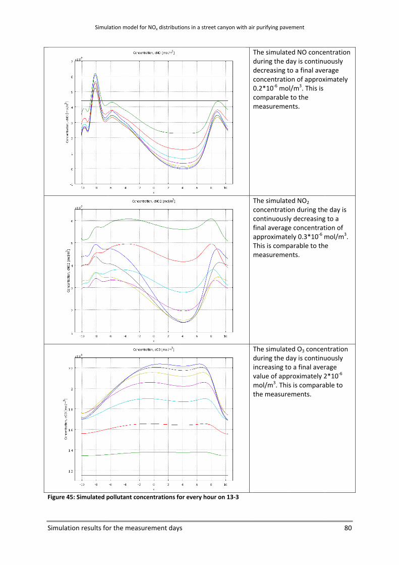
Simulatio
Figure 45
Simul
on results fo
5: Simulated p
ation model fo
or the measu
pollutant conc
or NOx distributi
urement days
centrations fo
ions in a street
s
or every hour
canyon with ai
on 13‐3
ir purifying pav
The simulateduring the ddecreasing tconcentratio0.2*10‐6 mocomparablemeasureme
The simulateconcentratiocontinuouslyfinal averageapproximateThis is compmeasureme
The simulateduring the dincreasing tovalue of appmol/m3. Thithe measure
ement
ed NO conceday is continuto a final aveon of approxl/m3. This is to the nts.
ed NO2 on during they decreasinge concentrately 0.3*10‐6 mparable to thnts.
ed O3 concenday is continuo a final averproximately 2s is comparaements.
80
entration uously erage ximately
e day is g to a tion of mol/m3. e
ntration uously rage 2*10‐6 able to

Simulatio
Figure 46
Simul
on results fo
6: Simulated p
ation model fo
or the measu
pollutant conc
or NOx distributi
urement days
centrations fo
ions in a street
s
or every hour
canyon with ai
on 16‐3
ir purifying pav
The averageconcentratiodecreases slof approximmol/m3. Thithe street m
The averageconcentratioat a an averaapproximateThe street mshowed a reNO2 concentday, which wthan the simconcentratio
The simulateduring the dincreasing tovalue of appmol/m3. Thimeasured inthe simulateconcentratio
ement
e simulated Non during thelightly to a fi
mately 0.2*10s is compara
measurement
e simulated Non is almost age value of ely 0.7*10‐6 mmeasuremenelatively constration durinwas slightly lmulated ons.
ed O3 concenday is continuo a final averproximately 2s behavior isn the street; ed increase ions is too hig
81
NO e day nal level 0‐6 able to ts.
NO2 constant
mol/m3. ts stant ng the ower
ntration uously rage 2*10‐6 s also however n O3 gh.
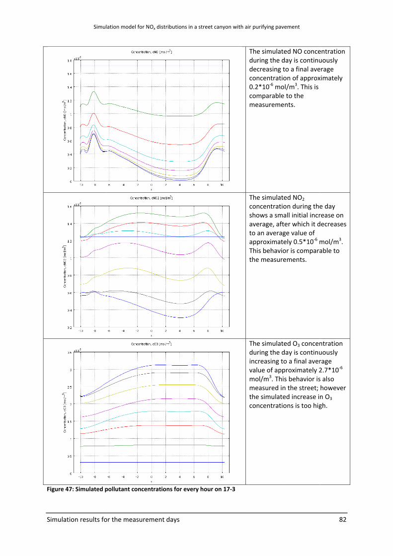
Simulatio
Figure 47
Simul
on results fo
7: Simulated p
ation model fo
or the measu
pollutant conc
or NOx distributi
urement days
centrations fo
ions in a street
s
or every hour
canyon with ai
on 17‐3
ir purifying pav
The simulateduring the ddecreasing tconcentratio0.2*10‐6 mocomparablemeasureme
The simulateconcentratioshows a smaaverage, aftto an averagapproximateThis behaviothe measure
The simulateduring the dincreasing tovalue of appmol/m3. Thimeasured inthe simulateconcentratio
ement
ed NO conceday is continuto a final aveon of approxl/m3. This is to the nts.
ed NO2 on during theall initial increr which it dge value of ely 0.5*10‐6 mor is comparaements.
ed O3 concenday is continuo a final averproximately 2s behavior isn the street; ed increase ions is too hig
82
entration uously erage ximately
e day rease on decreases
mol/m3. able to
ntration uously rage 2.7*10‐6 s also however n O3 gh.

Simulation model for NOx distributions in a street canyon with air purifying pavement
Simulation results for all scenarios 83
Appendix D: Simulation results for all scenarios In this appendix the graphs with the resulting concentrations for all scenarios are displayed. These graphs are used for the comparison with the standard scenario, in order to determine the effects of irradiance, wind speed, relative humidity, traffic density, and the active surface on the pollutant levels. For a quick comparison of the effects of these variables all graphs have the same scale, except when mentioned otherwise. The minima and maxima on the y‐axes have been chosen so that the results for all scenarios fit within the graph. In each figure, the NO concentrations are displayed in the top graphs, the NO2 concentrations in the middle and the O3 concentrations at the bottom. In these graphs, one line for each hour represents the pollutant concentrations at that moment during the day, ranging from 9:00h until 16:00h:
The concentrations at these times are displayed for a height in the street canyon of 1.50 m, except for Figure 49 and Figure 50, which display the concentrations at a height of 30 cm and 5 cm respectively. On the x‐axis of each graph in this appendix, the distance from the center of the street (x=0) is displayed in m.

Simulatio
Normal s
Figure 48
Simul
on results fo
street surfac
8: Pollutant le
ation model fo
or all scenario
ce
evels for the s
or NOx distributi
os
tandard scen
ions in a street
Activ
ario at a heig
canyon with ai
ve street surf
ht of 1.50 m
ir purifying pav
face
ement
84

Simulatio
Normal s
Figure 49
Simul
on results fo
street surfac
9: Pollutant le
ation model fo
or all scenario
ce
evels for the s
or NOx distributi
os
tandard scen
ions in a street
Activ
ario at a heig
canyon with ai
ve street surf
ht of 0.30 m
ir purifying pav
face
ement
85
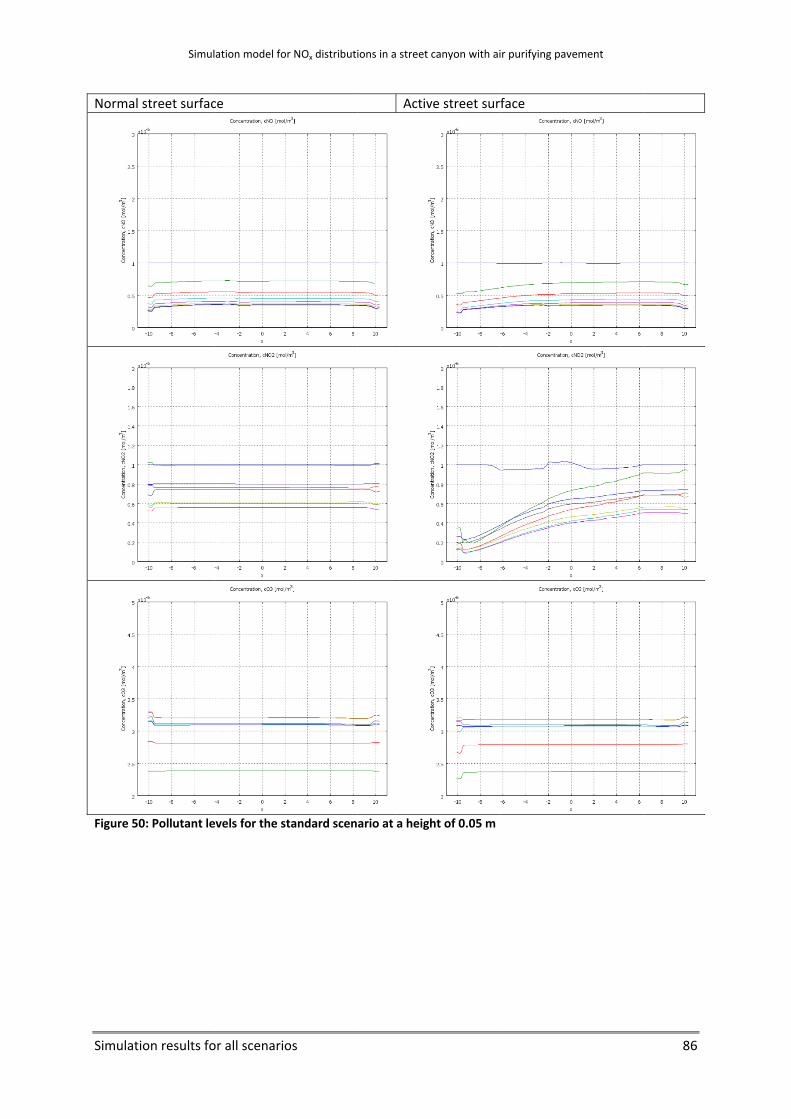
Simulatio
Normal s
Figure 50
Simul
on results fo
street surfac
0: Pollutant le
ation model fo
or all scenario
ce
evels for the s
or NOx distributi
os
tandard scen
ions in a street
Activ
ario at a heig
canyon with ai
ve street surf
ht of 0.05 m
ir purifying pav
face
ement
86

Simulatio
Normal s
Figure 51
Simul
on results fo
street surfac
1: Pollutant le
ation model fo
or all scenario
ce
evels for the h
or NOx distributi
os
high irradiance
ions in a street
Activ
e scenario
canyon with ai
ve street surf
ir purifying pav
face
ement
87

Simulatio
Normal s
Figure 52
Simul
on results fo
street surfac
2: Pollutant le
ation model fo
or all scenario
ce
evels for the lo
or NOx distributi
os
ow irradiance
ions in a street
Activ
e scenario
canyon with ai
ve street surf
ir purifying pav
face
ement
88

Simulatio
Normal s
Figure 53 Note thascenario
Simul
on results fo
street surfac
3: Pollutant le
at in Figure o.
ation model fo
or all scenario
ce
evels for the n
53, the sca
or NOx distributi
os
no wind scena
ales of the y
ions in a street
Activ
ario
y‐axes (conc
canyon with ai
ve street surf
centrations)
ir purifying pav
face
are differen
ement
nt than the
89
standard
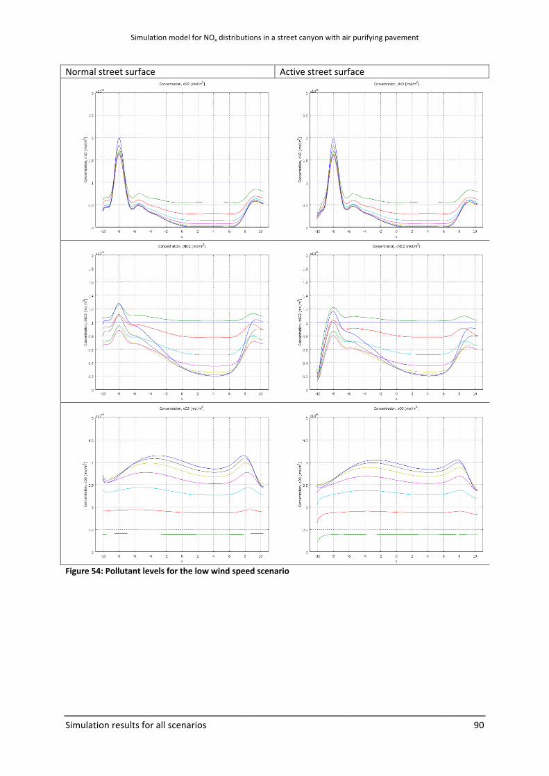
Simulatio
Normal s
Figure 54
Simul
on results fo
street surfac
4: Pollutant le
ation model fo
or all scenario
ce
evels for the lo
or NOx distributi
os
ow wind spee
ions in a street
Activ
ed scenario
canyon with ai
ve street surf
ir purifying pav
face
ement
90

Simulatio
Normal s
Figure 55
Simul
on results fo
street surfac
5: Pollutant le
ation model fo
or all scenario
ce
evels for the h
or NOx distributi
os
high wind spe
ions in a street
Activ
ed scenario
canyon with ai
ve street surf
ir purifying pav
face
ement
91
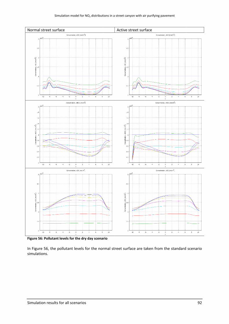
Simulatio
Normal s
Figure 56 In Figuresimulatio
Simul
on results fo
street surfac
6: Pollutant le
e 56, the polons.
ation model fo
or all scenario
ce
evels for the d
llutant levels
or NOx distributi
os
dry day scenar
s for the nor
ions in a street
Activ
rio
rmal street s
canyon with ai
ve street surf
surface are t
ir purifying pav
face
aken from t
ement
he standard
92
scenario
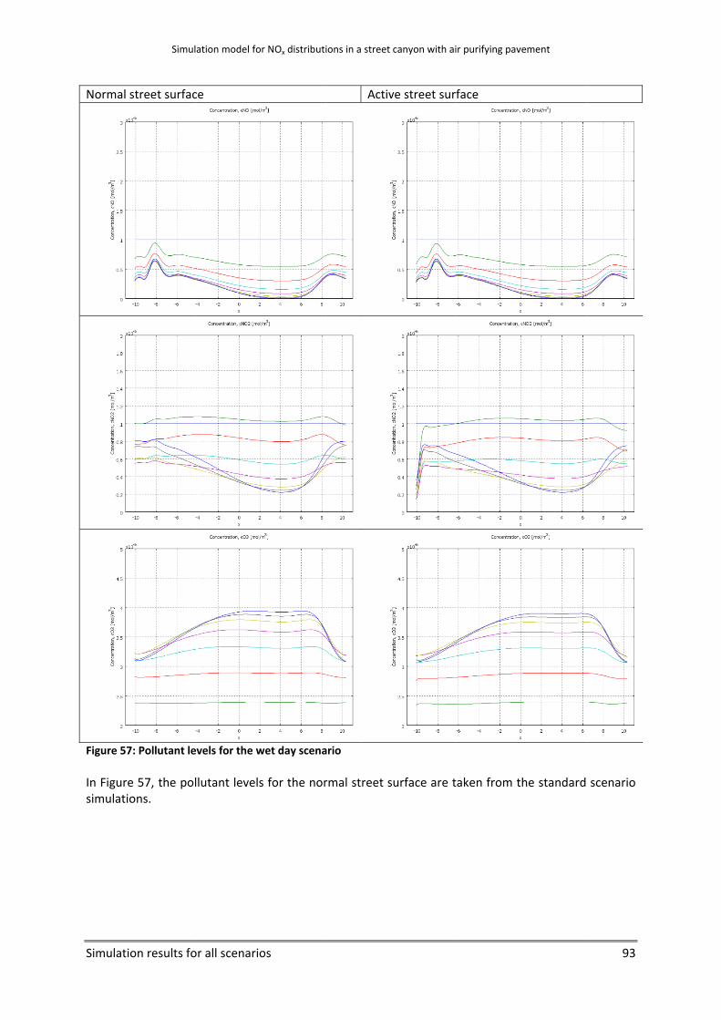
Simulatio
Normal s
Figure 57 In Figuresimulatio
Simul
on results fo
street surfac
7: Pollutant le
e 57, the polons.
ation model fo
or all scenario
ce
evels for the w
llutant levels
or NOx distributi
os
wet day scena
s for the nor
ions in a street
Activ
ario
rmal street s
canyon with ai
ve street surf
surface are t
ir purifying pav
face
aken from t
ement
he standard
93
scenario
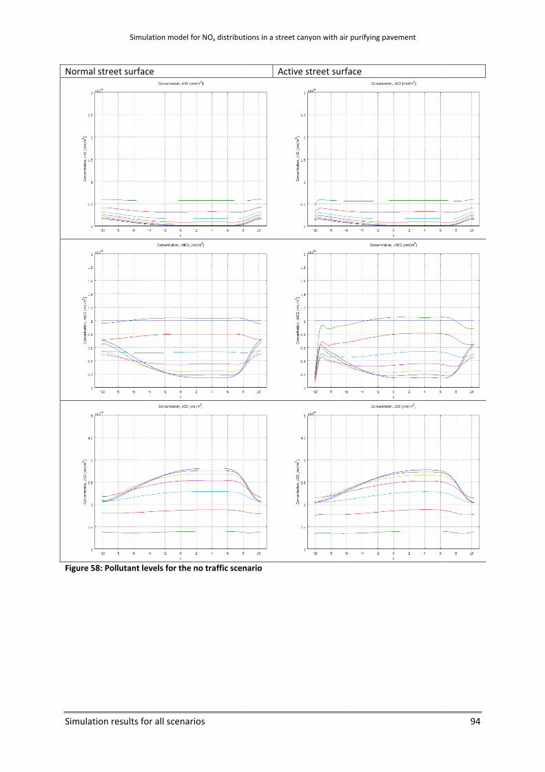
Simulatio
Normal s
Figure 58
Simul
on results fo
street surfac
8: Pollutant le
ation model fo
or all scenario
ce
evels for the n
or NOx distributi
os
no traffic scen
ions in a street
Activ
nario
canyon with ai
ve street surf
ir purifying pav
face
ement
94

Simulatio
Normal s
Figure 59
Simul
on results fo
street surfac
9: Pollutant le
ation model fo
or all scenario
ce
evels for the m
or NOx distributi
os
much traffic sc
ions in a street
Activ
cenario
canyon with ai
ve street surf
ir purifying pav
face
ement
95

Simulatio
Normal s
Figure 60 In Figurescenario
Simul
on results fo
street surfac
0: Pollutant le
e 60, the sco
ation model fo
or all scenario
ce
evels for the b
cale of the y
or NOx distributi
os
busy city scena
y‐axes (conc
ions in a street
Activ
ario
centrations)
canyon with ai
ve street surf
is 10 ten tim
ir purifying pav
face
mes as large
ement
e as in the
96
standard

Simulatio
Normal s
Figure 61
Simul
on results fo
street surfac
1: Pollutant le
ation model fo
or all scenario
ce
evels for the s
or NOx distributi
os
tandard scen
ions in a street
Activ
ario with Leig
canyon with ai
ve street surf
ghton constan
ir purifying pav
face
nts by Marsili
ement
‐Libelli (1996)
97
)
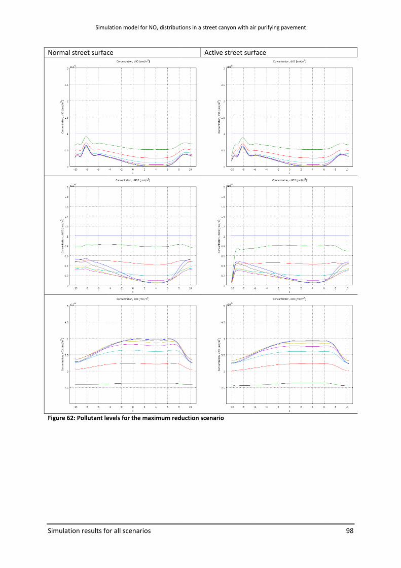
Simulatio
Normal s
Figure 62
Simul
on results fo
street surfac
2: Pollutant le
ation model fo
or all scenario
ce
evels for the m
or NOx distributi
os
maximum red
ions in a street
Activ
uction scenar
canyon with ai
ve street surf
rio
ir purifying pav
face
ement
98
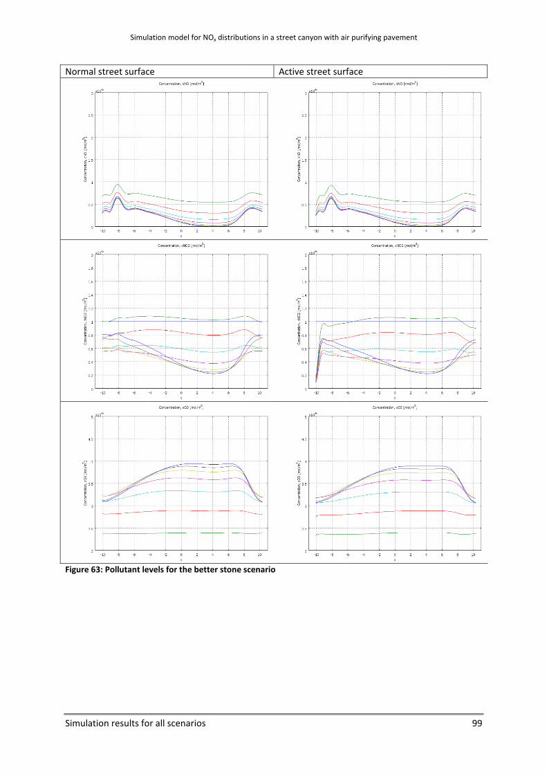
Simulatio
Normal s
Figure 63
Simul
on results fo
street surfac
3: Pollutant le
ation model fo
or all scenario
ce
evels for the b
or NOx distributi
os
better stone s
ions in a street
Activ
cenario
canyon with ai
ve street surf
ir purifying pav
face
ement
99


