FACULTY OF TECHNOLOGY
LUT ENERGY
ELECTRICAL ENGINEERING
MASTER’S THESIS
TECHNO-ECONOMIC FEASIBILITY OF NOVEL ON-LINECONDITION MONITORING METHODS IN LOW VOLTAGE
DISTRIBUTION NETWORKS
Examiners Prof. Jero Ahola
M.Sc. Tero Kaipia
Author Arto Ylä-Outinen
Lappeenranta 28.05.2012
Abstract
Lappeenranta University of Technology
Faculty of Technology
Electrical Engineering
Arto Ylä-Outinen
Techno-Economic Feasibility of Novel On-Line Condition Monitoring
Methods in Low Voltage Distribution Networks
Master’s thesis
2012
88 pages, 49 pictures, 8 tables and 1 appendix
Examiners: Prof. Jero Ahola and M.Sc. Tero Kaipia
Keywords: low voltage, distribution network, cable, fault, condition monitoring
The focus in this thesis is to study both technical and economical possibilities of
novel on-line condition monitoring techniques in underground low voltage dis-
tribution cable networks.
This thesis consists of literature study about fault progression mechanisms in
modern low voltage cables, laboratory measurements to determine the base and
restrictions of novel on-line condition monitoring methods, and economic evalu-
ation, based on fault statistics and information gathered from Finnish distribution
system operators.
This thesis is closely related to master’s thesis “Channel Estimation and On-line
Diagnosis of LV Distribution Cabling”, which focuses more on the actual condi-
tion monitoring methods and signal theory behind them.

Tiivistelmä
Lappeenrannan teknillinen yliopisto
Teknillinen tiedekunta
Sähkötekniikan koulutusohjelma
Arto Ylä-Outinen
Uudentyyppisten on-line kunnonvalvontamenetelmien teknis-taloudelliset
käyttömahdollisuudet pienjännitteisissä jakeluverkoissa
Diplomityö
2012
88 sivua, 49 kuvaa, 8 taulukkoa and 1 liite
Tarkastajat: professori Jero Ahola, diplomi-insinööri Tero Kaipia
Avainsanat: pienjännite, jakeluverkko, kaapeli, vika, kunnonvalvonta
Tämän työn tavoitteena on tutkia uudentyyppisten on-line kunnonvalvontamene-
telmien teknis-taloudellista soveltuvuutta pienjännitteisiin maakaapelijakelu-
verkkoihin.
Työ koostuu pienjännitteisten maakaapeleiden vikaantumismekanismeja käsitte-
levästä kirjallisuustutkimuksesta, uudentyyppisten kunnonvalvontamenetelmien
mahdollisuuksien määrittämisestä laboratoriomittauksin, sekä menetelmien so-
veltamisen taloudellisesta arvioinnista. Taloudellinen arviointi perustuu suoma-
laisilta jakeluverkkoyhtiöiltä saatuihin vikatilastoihin ja haastatteluihin koskien
käytössä olevia viankorjausmenetelmiä ja -käytäntöjä.
Tämä työ liittyy läheisesti diplomityöhön “Channel Estimation and On-line Dia-
gnosis of LV Distribution Cabling”, jossa uudentyyppisiä kunnonvalvontamene-
telmiä tarkastellaan tarkemmin signaalinkäsittelyn näkökulmasta.

This work was carried out in the Smart Grids and Energy Markets (SGEM) re-
search program coordinated by CLEEN Ltd. with funding from the Finnish
Funding Agency for Technology and Innovation, Tekes.
Tämä työ on tehty Smart Grids and Energy Markets (SGEM) tutkimusprojektin
yhteydessä, jota koordinoi CLEEN Oy ja rahoittaa Teknologian ja innovaatioi-
den kehittämiskeskus Tekes.
Table of ContentsAbbreviations and symbols ........................................................................................ 1
1 Introduction ....................................................................................................... 3
1.1 Background and purpose of the research ...................................................................... 3
1.2 Objectives ................................................................................................................... 4
2 LV distribution .................................................................................................. 5
2.1 Low voltage power cables ........................................................................................... 6
2.1.1 LV cable accessories .......................................................................................... 8
2.2 LVDC ....................................................................................................................... 10
3 Faults in underground LV cable network ........................................................12
3.1 Ageing ...................................................................................................................... 12
3.2 Damage mechanisms ................................................................................................. 14
3.2.1 Mechanical damage .......................................................................................... 14
3.2.2 Leakage currents .............................................................................................. 16
3.2.3 Treeing ............................................................................................................ 17
3.2.4 Arcing.............................................................................................................. 17
3.3 Examples of faulty LV cables .................................................................................... 19
3.4 Fault location ............................................................................................................ 21
3.4.1 Pre-location...................................................................................................... 21
3.4.2 Pin-pointing ..................................................................................................... 23
4 Condition measurements in underground cable network ...............................26
4.1 Insulation resistance .................................................................................................. 26
4.2 Dielectric loss factor .................................................................................................. 27
4.3 Partial discharge test .................................................................................................. 30
4.4 Differences between MV and LV networks ................................................................ 31
5 Novel on-line condition monitoring methods ...................................................33
5.1 Laboratory measurements .......................................................................................... 33
5.1.1 Test setup ......................................................................................................... 33
5.1.2 Long term water test ......................................................................................... 35
5.1.3 Progressive damaging of insulation................................................................... 40
5.1.4 Grid setup ........................................................................................................ 46
5.1.5 Conclusions ..................................................................................................... 50
5.2 Implementation to LV networks ................................................................................ 51
5.2.1 Communication between OCM system and network control software ................ 51
5.2.2 Description of the OCM system ........................................................................ 53
6 Economic evaluation of novel condition monitoring methods .........................57
6.1 Fault costs ................................................................................................................. 58
6.2 Benefits from OCM ................................................................................................... 61
6.3 OCM costs ................................................................................................................ 63
6.4 Application potential ................................................................................................. 66
7 Conclusions .......................................................................................................77
7.1 Technical aspects of OCM system ............................................................................. 77
7.2 Economic aspects of OCM system ............................................................................. 78
7.3 Further research topics .............................................................................................. 79
8 Summary ...........................................................................................................80
References .................................................................................................................81
APPENDIXES I Equations for break-even cost point graphs
1
Abbreviations and symbols
AC alternating current
AMCMK PVC insulated aluminum 1 kV power cable with concentric cop-
per conductor and PVC sheath
AMR automatic meter reading
AN annuity
AXMK XLPE insulated aluminum 1 kV power cable with PVC sheath
CIS customer information system
DC direct current
DMS distribution management system
DSO distribution system operator
EMA Energy Market Authority
GENELEC European Committee for Electrotechnical Standardization
HCC harm caused to the customers
HDPE high-density polyethylene
HV high voltage
HVDC high voltage direct current
IEC International Electrotechnical Commission
LDPE low-density polyethylene
LV low voltage
LVDC low voltage direct current
MV medium voltage
NIS network information system
OCM on-line condition monitoring
OIP oil-impregnated paper
PD partial discharge
PE polyethylene
PLC power line communication
PVC polyvinyl chloride
QMS quality management system
RH relative humidity
2
SCADA supervisory control and data acquisition
SGEM Smart Grids and Energy Markets
TDR time domain reflectometry
TSR transient recording system
UV ultraviolet
WTA willingness to accept
WTP willingness to pay
XLPE cross-linked polyethylene
List of symbols
A outage cost parameter € / kW
B outage cost parameter € / kWh
c unit cost € / h
f fault rate 1 / km, a
I investment €
l length km
n evaluation period a
P real power kW
p interest rate %
t time h
Subscripts
e equipment
f fault
l labor
pi planned interruption
r repair
3
1 Introduction
This thesis is a part of nationwide Smart Grids and Energy Markets (SGEM)
research. Thesis is closely related to master’s thesis “Channel Estimation and
On-line Diagnosis of LV Distribution Cabling”. In this thesis, the novel on-line
condition measurement (OCM) techniques for low voltage (LV) underground
cable network are evaluated from distribution system operators (DSO) point of
view. Thesis consists of literature study of fault mechanisms in LV underground
cable network, laboratory measurements and techno-economic evaluation, based
on statistics provided by Finnish DSOs.
1.1 Background and purpose of the research
Traditional concept of electric power system consists of centralized generation,
power transmission and distribution systems and passive loads. Electricity is
generated in large generating plants and transmitted via transmission network,
substations and distribution network to the end customers. Distribution network
consists of medium voltage (MV) network, usually rated 10 or 20 kV, and 400 V
LV networks, fed by MV network through secondary substations. Power flows
straightforwardly from higher voltage level to lower and thus, significance of LV
networks is much lower than MV networks because a fault in MV network af-
fects much larger group of customers. LV networks are also known to be more
reliable compared to MV networks due lower dielectric stress. Therefore, lots of
studies have been made to increase reliability of MV networks but very little
research have been done to increase reliability of LV networks.
Smart grid is a broad future network concept which includes active loads, energy
storages, distributed generation and communication between different network
components. Smart grid allows the consumers to participate in energy markets
by adjusting the consumption according to the current price of electricity, as well
as selling the surplus energy they produce by solar panels or by small scale wind
turbines. Electric vehicles can be used as energy storages, feeding the energy to
the network when power demand is high. Distributed generation, energy storag-
4
es, communication and intelligent control system allow independent local mi-
crogrids to maintain supply in the case of an interruption in feeding MV network
occurs.
Overall, the importance of LV networks will most probably raise in the future.
Novel techniques, such as low voltage direct current (LVDC), will increase pow-
er transmission capacity of present LV networks. Not only the power transmitted
to the customers will raise, but also the power transmitted from the customers, as
the customer-owned distributed generation and energy storages will become
more common. This will increase the power transmission within LV networks.
Therefore, demand of reliability of LV networks will most probably increase as
the impact of faults increase.
1.2 Objectives
Purpose of this thesis is to determine techno-economical potential of novel OCM
techniques in LV distribution network. Failure mechanisms and causes of fail-
ures in LV underground cable network are also studied, based on both literature
study and practical experiences from Finnish DSOs.
High frequency signal injection techniques are tested in laboratory environment
to determine the types and severities of defects that could possibly be detected
with such condition monitoring techniques. The effect of insulation material is
tested by performing the tests with two different LV cables; cross-linked poly-
ethylene (XLPE) insulated AXMK and polyvinylchloride (PVC) insulated
AMCMK. Branches and joints are added to determine the functionality of meas-
urement techniques in more complex network topologies.
Economic potential of OCM system is determined by assessing the potential cost
savings it generates through decreasing the number of unexpected faults annual-
ly. Evaluation is based on fault statistics and information gathered from Finnish
DSOs.
5
2 LV distribution
Electricity distribution networks connect the end customers to the transmission
network. Distribution network consists of primary HV/MV substations, MV
network, secondary MV/LV substations and LV networks. At primary substa-
tions HV, used in longer distance power transmission, is transformed to MV and
fed to the MV network. Distribution transformers inside secondary substations
transform MV to LV, and feed the LV networks, where the most of end custom-
ers are connected to. In Finnish distribution system, the most commonly used
voltage in LV networks is 3-phase 230/400 VAC. Also 690 V and 1 kV phase-
to-phase low voltages are used in some special cases, the former is usually used
in factories and latter in some distribution networks. (Lakervi & Partanen, 2009)
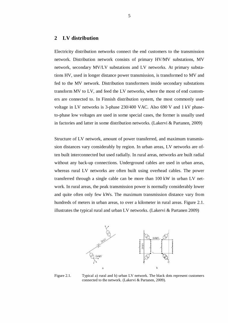
Structure of LV network, amount of power transferred, and maximum transmis-
sion distances vary considerably by region. In urban areas, LV networks are of-
ten built interconnected but used radially. In rural areas, networks are built radial
without any back-up connections. Underground cables are used in urban areas,
whereas rural LV networks are often built using overhead cables. The power
transferred through a single cable can be more than 100 kW in urban LV net-
work. In rural areas, the peak transmission power is normally considerably lower
and quite often only few kWs. The maximum transmission distance vary from
hundreds of meters in urban areas, to over a kilometer in rural areas. Figure 2.1.
illustrates the typical rural and urban LV networks. (Lakervi & Partanen 2009)
Figure 2.1. Typical a) rural and b) urban LV network. The black dots represent customersconnected to the network. (Lakervi & Partanen, 2009).
6
2.1 Low voltage power cables
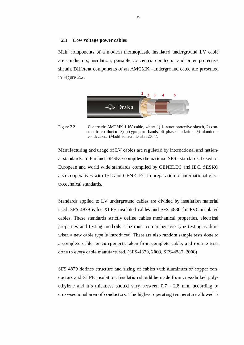
Main components of a modern thermoplastic insulated underground LV cable
are conductors, insulation, possible concentric conductor and outer protective
sheath. Different components of an AMCMK –underground cable are presented
in Figure 2.2.
Figure 2.2. Concentric AMCMK 1 kV cable, where 1) is outer protective sheath, 2) con-centric conductor, 3) polypropene bands, 4) phase insulation, 5) aluminumconductors. (Modified from Draka, 2011).
Manufacturing and usage of LV cables are regulated by international and nation-
al standards. In Finland, SESKO compiles the national SFS –standards, based on
European and world wide standards compiled by GENELEC and IEC. SESKO
also cooperatives with IEC and GENELEC in preparation of international elec-
trotechnical standards.
Standards applied to LV underground cables are divided by insulation material
used. SFS 4879 is for XLPE insulated cables and SFS 4880 for PVC insulated
cables. These standards strictly define cables mechanical properties, electrical
properties and testing methods. The most comprehensive type testing is done
when a new cable type is introduced. There are also random sample tests done to
a complete cable, or components taken from complete cable, and routine tests
done to every cable manufactured. (SFS-4879, 2008, SFS-4880, 2008)
SFS 4879 defines structure and sizing of cables with aluminum or copper con-
ductors and XLPE insulation. Insulation should be made from cross-linked poly-
ethylene and it’s thickness should vary between 0,7 - 2,8 mm, according to
cross-sectional area of conductors. The highest operating temperature allowed is
7
90 °C. Thickness of outer sheath, usually made from PVC- or PE- based thermo-
plastic, should be 1,8 - 3,1 mm. (SFS-4879, 2008)
SFS 4880 defines structure, sizing and testing of cables with PVC insulation and
-sheath. Extruded insulation thickness should vary between 1,0 - 1,6 mm, ac-
cording to cross-sectional area of conductors. The highest operating temperature
allowed is 70 °C. Thickness of outer PVC- sheath should be 1,8 - 3,2 mm. (SFS-
4880, 2008)
Routine tests consist of conductor tests, spark tests and high-voltage test with
3 kV AC for 5 min, or 10 kV DC for 15 min. During the type testing, cable is
immersed to water of 70 °C, and insulation resistance is then measured. Cable is
left under the water for 1 h, followed by voltage test with 4 kV AC for 4 h. (SFS-
4880, 2008)
Some cables have concentric conductor running between outer sheath and insula-
tion, which is made from copper wires. Concentric conductor is connected to the
earth potential and it provides protection against electric shock, in case the cable
sheath and insulation has been penetrated, for example, with metallic shovel.
Fault current then flows from phase conductor to the concentric conductor, in-
stead of flowing through the person holding the shovel. (Suntila, 2009)
White polypropene tapes are used for keeping the individual wires together dur-
ing the manufacturing process. They also isolate the main insulation material
from the hot thermoplastic when the cable sheath is being extruded. Tapes also
help the cable to withstand the forces caused by high current short circuits. Con-
centric cables have two layers of polypropene tapes, one on each side of the con-
centric conductor. (Suntila, 2009)
Conductors are usually made from annealed aluminum strands. Conductors are
round shaped with small cross-sectional areas, usually under 25 mm2, and sector
shaped with larger cross-sectional areas. Cross-sectional area of conductors, to-

8
gether with insulation material used, define the maximum continuous and fault
currents allowed through the cable. (SFS-4879, 2008, SFS-4880, 2008)
The most common cable types used in Finnish underground LV distribution ca-
ble network are PVC- and XLPE –insulated aluminum cables. The main proper-
ties of these cables are presented in Table 2.1.
Table 2.1. The main properties of the AXMK and AMCMK LV cables.
National type code AXMK AMCMK
Sheath material PVC PVC
Insulation material XLPE PVC
Conductor material aluminium aluminium
Number of conductors 4 3 + 1
Concentric conductor - copper strings
In this thesis, cables presented in Table 2.1 will be called by their national type
codes; AXMK and AMCMK.
There are also cables with two separate sheath layers, for example, Draka
AMCMK-HD with inner PVC- and outer PE -sheaths (Draka, 2011). These dou-
ble sheathed cables are designed especially for rough environments and to be
installed using a cable plough. By using different materials in different sheaths,
advantages of both materials can be utilized. Downside of double sheathed ca-
bles is price. For example, 95 mm2 double sheathed XLPE insulated cable is
about 20 % more expensive than single sheathed version (Pavo, 2011).
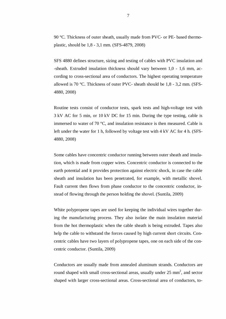
2.1.1 LV cable accessories
Cable accessories are needed to join cables to an another cable or to a device,
such as a fuse base or a transformer pole. Connection between conductor and a
cable joint or a lug can be done by bolting or by crimping. Joints are protected
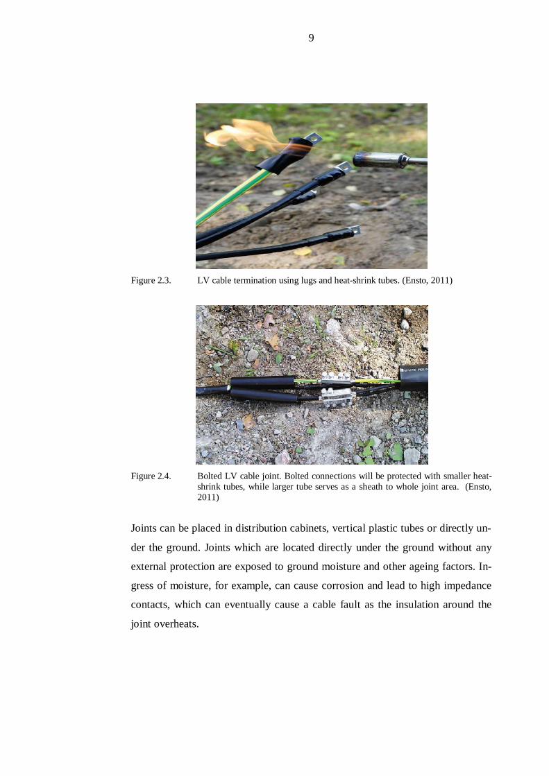
using heat-shrink tubes or resin casts. LV cable termination using lugs and heat-
shrink tubes is presented in Figure 2.3 and bolted LV cable joint in Figure 2.4.
9
Figure 2.3. LV cable termination using lugs and heat-shrink tubes. (Ensto, 2011)
Figure 2.4. Bolted LV cable joint. Bolted connections will be protected with smaller heat-shrink tubes, while larger tube serves as a sheath to whole joint area. (Ensto,2011)
Joints can be placed in distribution cabinets, vertical plastic tubes or directly un-
der the ground. Joints which are located directly under the ground without any
external protection are exposed to ground moisture and other ageing factors. In-
gress of moisture, for example, can cause corrosion and lead to high impedance
contacts, which can eventually cause a cable fault as the insulation around the
joint overheats.
10
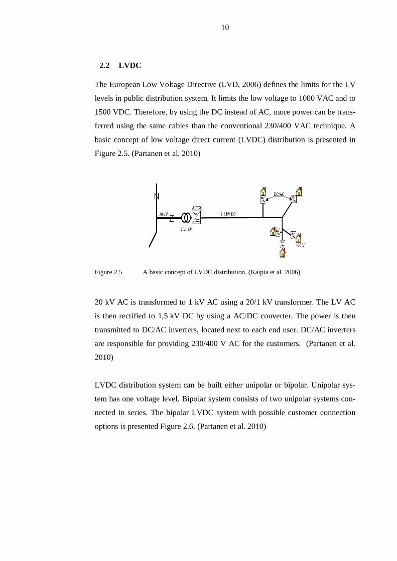
2.2 LVDC
The European Low Voltage Directive (LVD, 2006) defines the limits for the LV
levels in public distribution system. It limits the low voltage to 1000 VAC and to
1500 VDC. Therefore, by using the DC instead of AC, more power can be trans-
ferred using the same cables than the conventional 230/400 VAC technique. A
basic concept of low voltage direct current (LVDC) distribution is presented in
Figure 2.5. (Partanen et al. 2010)
Figure 2.5. A basic concept of LVDC distribution. (Kaipia et al. 2006)
20 kV AC is transformed to 1 kV AC using a 20/1 kV transformer. The LV AC
is then rectified to 1,5 kV DC by using a AC/DC converter. The power is then
transmitted to DC/AC inverters, located next to each end user. DC/AC inverters
are responsible for providing 230/400 V AC for the customers. (Partanen et al.
2010)
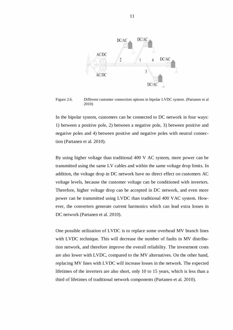
LVDC distribution system can be built either unipolar or bipolar. Unipolar sys-
tem has one voltage level. Bipolar system consists of two unipolar systems con-
nected in series. The bipolar LVDC system with possible customer connection
options is presented Figure 2.6. (Partanen et al. 2010)
11
Figure 2.6. Different customer connection options in bipolar LVDC system. (Partanen et al2010)
In the bipolar system, customers can be connected to DC network in four ways:
1) between a positive pole, 2) between a negative pole, 3) between positive and
negative poles and 4) between positive and negative poles with neutral connec-
tion (Partanen et al. 2010).
By using higher voltage than traditional 400 V AC system, more power can be
transmitted using the same LV cables and within the same voltage drop limits. In
addition, the voltage drop in DC network have no direct effect on customers AC
voltage levels, because the customer voltage can be conditioned with inverters.
Therefore, higher voltage drop can be accepted in DC network, and even more
power can be transmitted using LVDC than traditional 400 VAC system. How-
ever, the converters generate current harmonics which can lead extra losses in
DC network (Partanen et al. 2010).
One possible utilization of LVDC is to replace some overhead MV branch lines
with LVDC technique. This will decrease the number of faults in MV distribu-
tion network, and therefore improve the overall reliability. The investment costs
are also lower with LVDC, compared to the MV alternatives. On the other hand,
replacing MV lines with LVDC will increase losses in the network. The expected
lifetimes of the inverters are also short, only 10 to 15 years, which is less than a
third of lifetimes of traditional network components (Partanen et al. 2010).

12
3 Faults in underground LV cable network
Underground cable faults can be divided to instant abrupt faults, for example,
caused by excavator, and to slowly developing incipient faults. In this thesis, the
focus is on the incipient faults. Incipient damages in the cable will slowly devel-
op to electric faults, leading to a breakdown in the insulation system, and causing
a power outage. Many factors govern the development speed of an electric fault
due to an incipient damage in a cable. Fault development speed is dependent on,
for example, the environmental conditions, such as ground moisture and impuri-
ties, and the load profile of the cable.
3.1 Ageing
Underground cables experience numerous ageing factors which, over the time,
cause irreversible changes in the cable insulation system. Cable joints and termi-
nations are also affected, which can lead to corrosion and high impedance con-
tacts. In Table 3.1, ageing factors are categorized to thermal, electrical, environ-
mental and mechanical factors.
Table 3.1. Ageing factors in underground cable insulation system (Densley, 2001).
Thermal Electrical Environmental Mechanical
Maximum Tempera-ture Voltage Oxygen Bending
Ambient Tempera-ture max / min Frequency Water / humidity Tension
Temperature gradient Current Chemicals Compression
Temperature cycling (Radiation) Vibration
Torsion
These factors alone, or acting synergistically, can induce changes in the insula-
tion material of the cables. This type of ageing is referred to as intrinsic ageing
and it could have effect on large volume of insulation, such as overheating due
overloading the cable. Ageing factors also interact with contaminants, defects
and other localized changes in insulation structure, causing degradation of insu-
lation. This type of ageing is referred to as extrinsic ageing. Degradation usually
13
starts at localized regions, and gradually propagating through insulation. (Dens-
ley 2001).
Maximum temperature, to which cable is exposed, is determined by ambient
temperature and by the maximum current transferred through the cable. There-
fore, overloading can cause insulation temperature to exceed the highest opera-
tion temperature set by cable manufacturer. This will accelerate structural ageing
in polymers, and therefore, shorten the life of the cable insulation significantly.
Heat will also accelerate other ageing factors, like chemical reactions. Cables
with XLPE insulation withstand higher temperatures than PVC insulated cables
(Kärnä 2005).
Variation of current transferred through the cable causes temperature cycling.
This recurring heating and cooling causes thermal expansion and –contraction,
which can lead to movement in cable interfaces. Movement can eventually lead
to high impedance contacts and excessive heating in cable joints and termina-
tions (Densley 2001).
Underground cables are exposed to soil moisture and possible chemicals. Proper-
ties of polymers, used in outer sheath and insulation, determine cables ability to
withstand moisture and chemicals. Chemical degradation is caused by formation
of free radicals which leads to un-zipping and breaking the polymer chains. This
reaction can be initiated internally by thermal or mechanical means, by oxidizing
reaction, by hydrolysis or by UV ionizing reaction. Chemicals in soil can also
damage the cable directly when cable is installed in polluted environment. PVC
has good resistance against chemicals, but it permits more diffusion of water
through than PE (Suntila 2009).
Electrical stress from normal operating voltage to LV cable insulation is very
low. Thickness of insulation is determined rather from mechanical aspects than
from dielectric strength requirements, and it is considerably oversized from die-
lectric strength point of view. However, in case of LV underground cable net-
14
work is fed from overhead MV line, direct lightning strike to the transformer or
to nearby MV lines can damage already aged cable or defected cable joint. Finn-
ish DSOs have practical experience where especially cable joints have been de-
stroyed after a thunderstorm.
UV radiation causes ageing in exposed polymers by breaking the polymer chains
(Aro et al. 2003). Underground cables are safe from UV radiation, except for
short lengths, for example, from pole-mounted transformer to under the ground.
Carbon black is added to polymers during the manufacturing process, in order to
decrease the effect from UV radiation (Suntila 2009).
3.2 Damage mechanisms
Actual damage mechanism for incipient faults in LV underground cables is rela-
tively little studied phenomena, whereas lots of material can be found regarding
fault propagation in MV or HV cables. Fault propagation in MV or HV cables is
usually more straightforward due greater voltage stress over the insulation. Prac-
tical experiences from LV cable faults where fuse is ruptured and then, after it
has been replaced, fault have disappeared for considerably long periods of time,
shows their unstable nature.
3.2.1 Mechanical damage
Cable is exposed to significant mechanical stress during the cable installation
process. Installation at sub-zero temperatures increases the stress, especially to
thermoplastics used in cable insulation and sheath. Bending and torsion can
cause defects in cable sheath as the thermoplastic cracks due breaking of the pol-
ymer bonds under tension. Cross-linking improves the thermoplastics mechani-
cal durability. Conductors can also be damaged due excessive mechanical stress.
Therefore, cable manufacturer defines the smallest bending radius and maximum
pulling force allowed to different cables. (Kärnä 2005).
LV cables can be installed by traditional trench excavating or by ploughing.
When installing to trench, cable has to be pulled along the ground. Cable sheath
15
can therefore be damaged by sharp stone or by other sharp object left unnoticed.
Nearby stones can damage the cable also afterward due pressure from the soil
filled back to the trench, or due ground movement caused by ground frost.
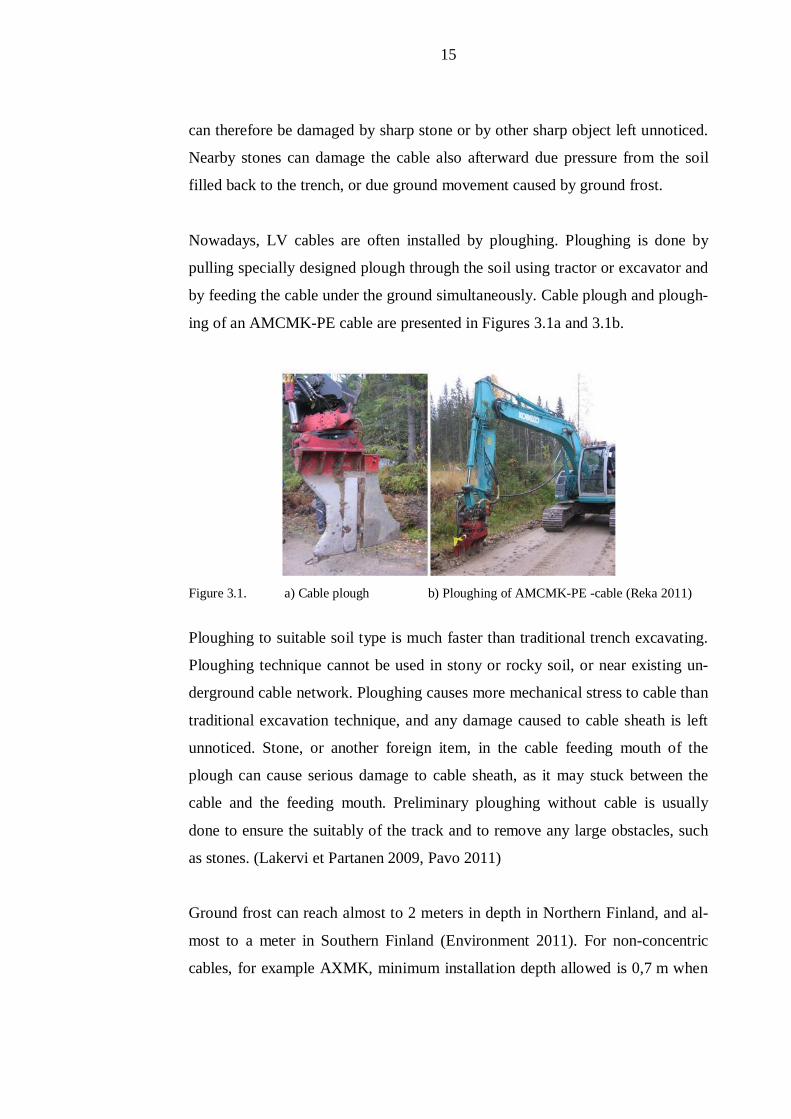
Nowadays, LV cables are often installed by ploughing. Ploughing is done by
pulling specially designed plough through the soil using tractor or excavator and
by feeding the cable under the ground simultaneously. Cable plough and plough-
ing of an AMCMK-PE cable are presented in Figures 3.1a and 3.1b.
Figure 3.1. a) Cable plough b) Ploughing of AMCMK-PE -cable (Reka 2011)
Ploughing to suitable soil type is much faster than traditional trench excavating.
Ploughing technique cannot be used in stony or rocky soil, or near existing un-
derground cable network. Ploughing causes more mechanical stress to cable than
traditional excavation technique, and any damage caused to cable sheath is left
unnoticed. Stone, or another foreign item, in the cable feeding mouth of the
plough can cause serious damage to cable sheath, as it may stuck between the
cable and the feeding mouth. Preliminary ploughing without cable is usually
done to ensure the suitably of the track and to remove any large obstacles, such
as stones. (Lakervi et Partanen 2009, Pavo 2011)
Ground frost can reach almost to 2 meters in depth in Northern Finland, and al-
most to a meter in Southern Finland (Environment 2011). For non-concentric
cables, for example AXMK, minimum installation depth allowed is 0,7 m when

16
no external protection is used (SFS-6000-8-814 2007), which is close to an aver-
age installation depth in practice (Pavo 2011). Ground frost generates movement
and pressure in the soil, causing mechanical stress to cables and cable joints bur-
ied under the ground.
The roots of trees and plants can also damage underground cables. The fault sta-
tistics from the DSOs showed that there were cases, where the same distribution
cabinet had to be replaced twice, because of the roots of nearby tree had dam-
aged also the new cabinet and cabling installed to the same location. Rodents are
also known to damage the cables.
3.2.2 Leakage currents
Leakage current occur when conductive path is formed through cable insulation
between phase conductor and concentric conductor or mass of earth. Many fac-
tors can cause the conductive path to form through cable sheath and insulation,
but moisture is the key element in most cases. Mechanical damage to cable, or
incorrectly done cable joint can allow water to penetrate through insulation. Im-
pedance of the conductive path first limit the leakage current under the tripping
point of protective device, in case of LV, typically a fuse. Therefore, the current
leakage stay undetected until partial discharge activity occurs over the time.
Experiments with oil-impregnated paper (OIP) insulated LV cables show that
shortly after the leakage current reached 100 mA, intensive discharges occurred
leading to catastrophic failure of the cable. Study also revealed strong relation
between conductor temperature and magnitude of leakage current. Especially
rapid increase of temperature has been shown to increase the leakage current
through insulation (Rowland et Wang 2007).
Although the results from OIP insulated LV cable experiments cannot be directly
applied to thermoplastic insulated cables, it can be assumed that leakage current
will cause discharges also in thermoplastic insulation. Magnitude of leakage cur-
17
rent in real installation conditions will most probably raise over the time due
ingress of moisture and deterioration of insulation.
3.2.3 Treeing
Although the treeing phenomena in polymer insulating materials have been stud-
ied for decades, the exact build-up mechanisms of trees remains somewhat un-
known. Water tree is tree shaped microscopic formation of water, which devel-
ops through the insulation material. Water trees are formed due presence of wa-
ter and electric field and they grow in parallel with electric field. Required elec-
tric field intensity for water trees to grow is commonly considered to be at least
1 kV/mm and RH should be over 70 % (Kärnä 2005). Water can get to insulation
through damaged cable sheath, incorrectly done installation of cable or cable
joint, or by penetrating the sheath by diffusion. PE and XLPE allow less water
through by diffusion than PVC (Aro et. al 2003).
Water tree decreases cable’s dielectric strength, but it would not necessarily lead
to breakdown in insulation. Breakdown strength of insulation penetrating water
tree is often at least 2 kV/mm, therefore, water trees do not cause a serious threat
to LV cables. On the other hand, water and chemical compounds initiate elec-
trolysis, chemical reactions and oxidation around the tree area. This leads to de-
terioration of insulation material (Kärnä 2005).
3.2.4 Arcing
An arc is electrical discharge between two electrodes through gas, liquid or solid
material. Arcs can initiate when the voltage stress over the insulation exceeds
dielectric strength of insulation. It has shown that 95 % dielectric strength level
for modern thermoplastic-insulated LV underground cables are at least 15 kV,
when 50 Hz AC test voltage is used (Suntila 2009).
According to simulations done by Hannu Mäkelä, the highest overvoltage level,
caused by direct lightning strike to pole-mounted distribution transformer, in
studied LV underground cable network was 7,2 kV (Mäkelä 2009). Comparing
18
this result to dielectric strength of LV cables, it can be seen that modern intact
thermoplastic-insulated LV cables will probably withstand the voltage stress
from direct lightning strike to the distribution transformer.
However, momentary discharges can initiate much lower voltage level when
cable is damaged. Ingress of moisture and impurities can form conductive path
through insulation, causing leakage current to flow through insulation. When the
magnitude of leakage current exceeds certain level, transitory discharges begin to
occur (Rowland et Wang 2007).
Insulation thickness in LV cables is oversized, compared to dielectric stress
caused by low voltage. Thickness of insulation is determined by mechanical du-
rability, rather than electrical factors. This causes the incipient LV cable faults to
be often non-linear and unstable. In Table 3.2. incipient LV cable faults have
been classified by their characteristics (Livie et al. 2008).
Table 3.2. Classification of incipient LV cable faults (Livie et al. 2008).
Condition Classification Characteristic
Unstable / Non-linear Transitory Irregular voltage dips
Intermittent Irregular fuse operations
Persistent Repetitive fuse operations
Stable / Linear Permanent Open circuit / Solid welds
Gradually developing incipient LV cable faults often initiate at transitory state.
Flickering lights can be first sign of a emerging cable fault, since momentary
arcing generates voltage transients. Severity and frequency of arcing depends on
the state of conductive fault tracks formed inside the insulation, moisture and
amount of impurities in faulty area. Those arcs self-extinguish, but permanent
damage to cable insulation is done, since the arcs create conductive surface fault
tracks inside the insulation. Therefore, unstable faults gradually develop toward
stable permanent state, and the fault current eventually ruptures the fuse. Unsta-
ble fault can exist for days, or even for months, until it becomes permanent.
19
Practical experiences from DSOs support this theory (Gammon et. Matthews
1999, Clegg, 1994).
3.3 Examples of faulty LV cables
Following figures present three samples, taken from real faulty LV cables. Sam-
ples were provided by a Finnish DSO, along with assumptions of root cause for
each fault.
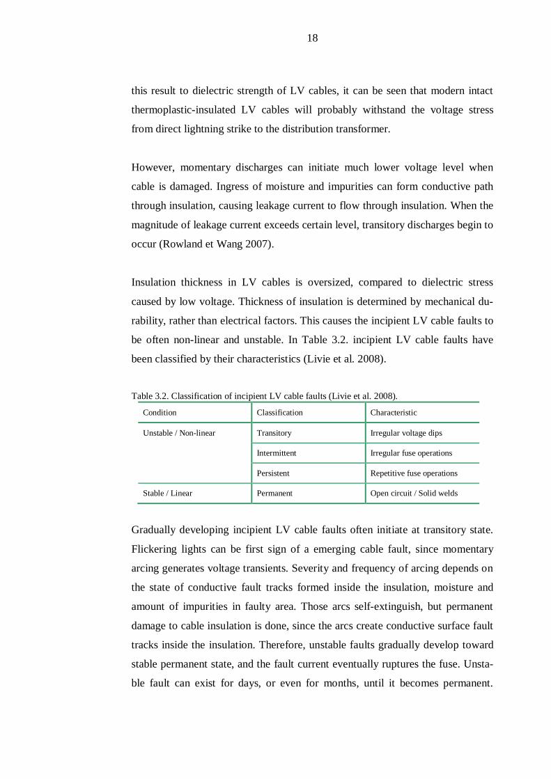
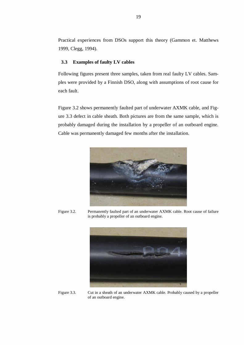
Figure 3.2 shows permanently faulted part of underwater AXMK cable, and Fig-
ure 3.3 defect in cable sheath. Both pictures are from the same sample, which is
probably damaged during the installation by a propeller of an outboard engine.
Cable was permanently damaged few months after the installation.
Figure 3.2. Permanently faulted part of an underwater AXMK cable. Root cause of failureis probably a propeller of an outboard engine.
Figure 3.3. Cut in a sheath of an underwater AXMK cable. Probably caused by a propellerof an outboard engine.
20
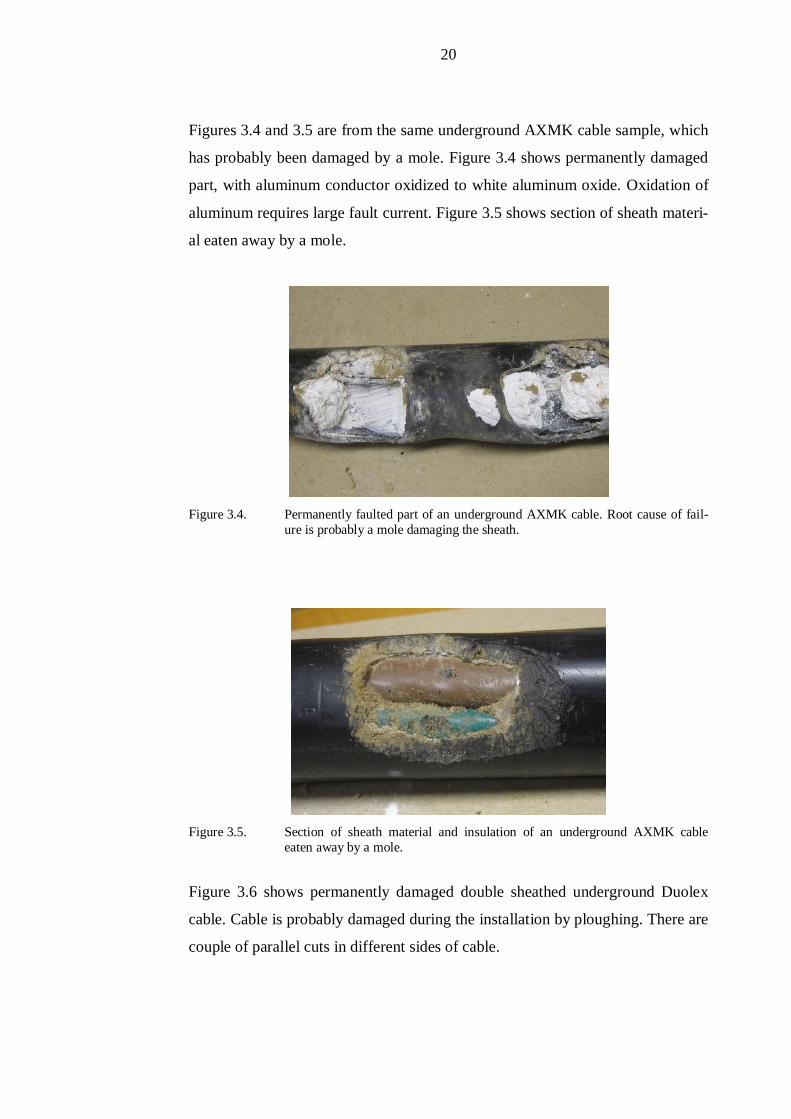
Figures 3.4 and 3.5 are from the same underground AXMK cable sample, which
has probably been damaged by a mole. Figure 3.4 shows permanently damaged
part, with aluminum conductor oxidized to white aluminum oxide. Oxidation of
aluminum requires large fault current. Figure 3.5 shows section of sheath materi-
al eaten away by a mole.
Figure 3.4. Permanently faulted part of an underground AXMK cable. Root cause of fail-ure is probably a mole damaging the sheath.
Figure 3.5. Section of sheath material and insulation of an underground AXMK cableeaten away by a mole.
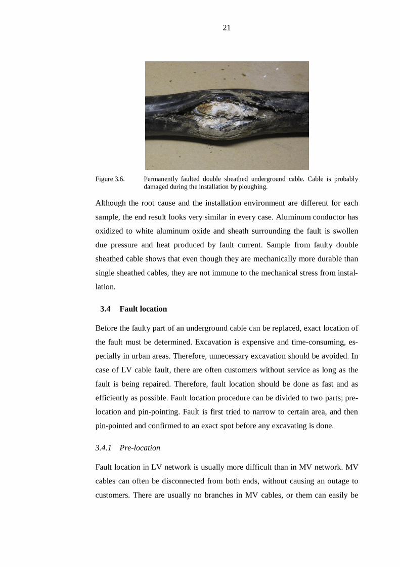
Figure 3.6 shows permanently damaged double sheathed underground Duolex
cable. Cable is probably damaged during the installation by ploughing. There are
couple of parallel cuts in different sides of cable.
21
Figure 3.6. Permanently faulted double sheathed underground cable. Cable is probablydamaged during the installation by ploughing.
Although the root cause and the installation environment are different for each
sample, the end result looks very similar in every case. Aluminum conductor has
oxidized to white aluminum oxide and sheath surrounding the fault is swollen
due pressure and heat produced by fault current. Sample from faulty double
sheathed cable shows that even though they are mechanically more durable than
single sheathed cables, they are not immune to the mechanical stress from instal-
lation.
3.4 Fault location
Before the faulty part of an underground cable can be replaced, exact location of
the fault must be determined. Excavation is expensive and time-consuming, es-
pecially in urban areas. Therefore, unnecessary excavation should be avoided. In
case of LV cable fault, there are often customers without service as long as the
fault is being repaired. Therefore, fault location should be done as fast and as
efficiently as possible. Fault location procedure can be divided to two parts; pre-
location and pin-pointing. Fault is first tried to narrow to certain area, and then
pin-pointed and confirmed to an exact spot before any excavating is done.
3.4.1 Pre-location
Fault location in LV network is usually more difficult than in MV network. MV
cables can often be disconnected from both ends, without causing an outage to
customers. There are usually no branches in MV cables, or them can easily be

22
disconnected. LV cables are often branched, and disconnecting them could be
time-consuming. Also the unstable nature of faults in LV cables can cause diffi-
culties in fault locating, or even make it impossible until the fault becomes per-
manent (Clegg 1994).
Fault can often be narrowed to certain area with simple measurements and logi-
cal reasoning. Blown fuses, and information about which customers are out of
service, narrows the possible fault location to certain area. Number of fuses
blown and simple voltage measurements reveal type of the fault, such as one- or
multi-phase open circuit, phase-to-phase short circuit, or phase-to-earth fault
(Clegg 1994).
Sophisticated analyzers, such as a time domain reflectometer (TDR) -device, can
also be used for pre-locating the faulty spot of cable. TDR device is connected to
a faulty cable at secondary substation or at distribution cabinet, and it launches a
pulse into the faulty cable. This pulse is completely or partly reflected from any
impedance mismatch it encounters, such as joints, end of branches, or faults.
Distance of mismatches can then be calculated by assuming the velocity of sig-
nal propagation to be constant for a given cable. Interpretation of TDR trace re-
quires skill, and every branch in network causes attenuation in signal and more
complex trace. Therefore, high impedance faults located far away from TDR
device can remain undetected, since their weak trace gets lost in the noise pro-
duced by branches and other impedance mismatches (Clegg 1994).
On many occasions, it is possible to treat the fault by repeated re-energizing the
faulty cable, in order to create a clear open circuit situation, or low-impedance
short circuit. TDR trace should be recorded before the re-energizing is done, so
any change in trace after re-energizing is done can give away the location of the
fault. Re-energizing can be done by replacing the fuses, or by specially designed
fault re-energizing device with build-in circuit-breaker (Clegg 1994).
23
Ongoing expansion of AMR (automatic meter reading) network will speed up
the fault locating process in the future, as soon as the full potential of AMR me-
ters can be utilized. Meters can send an alarm when individual customer is out of
service. Therefore, by knowing which customers are affected by the fault, the
network operator can quickly narrow the fault to certain area even before dis-
patching the workgroup. AMR meters can also detect potentially hazardous bro-
ken neutral situation, which can cause overvoltage to occur.
3.4.2 Pin-pointing
Extent of pin-pointing work to be done, depends on the accuracy and extension
of pre-location. The most simplest case is when there is an obvious cause of
fault, for example, sign of recent excavating work within the pre-located fault
area. Excavator can cause also an incipient fault by damaging the cable sheath,
but not completely destroying the cable and causing an abrupt fault. Fault can
then develop, depending on severity of fault and soil conditions, within days or
even months after cable sheath is originally damaged.
Heat, produced by fault current, can melt snow on the ground and thus give away
the fault location. Burning of insulation or cable sheath materials generate cer-
tain odor, which can be detected by special analyzer or by a trained dog. In some
cases, noise produced by arcing is loud enough to be heard on the ground, when
the faulty cable is being re-energized (Clegg 1994).
When no visual or otherwise obvious clue about fault location is available, fault
can be tried to pin-point by injecting audio frequency signals to faulty cable
while following the cable route on the ground and using hand-held receivers to
receive them. Fault can be detected from discontinuance of received signal. Au-
dio frequency method is suitable only for detecting low-impedance-, or clear
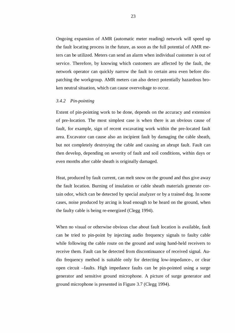
open circuit –faults. High impedance faults can be pin-pointed using a surge
generator and sensitive ground microphone. A picture of surge generator and
ground microphone is presented in Figure 3.7 (Clegg 1994).
24
Figure 3.7. SSG 500 Surge Voltage Generator and BM 30 Ground Microphone, equippedwith digital Universal Locator UL 30. (Baur)
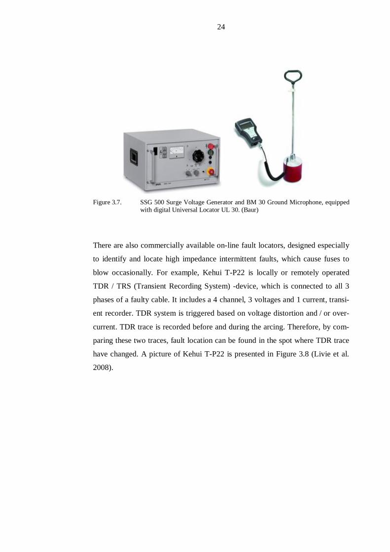
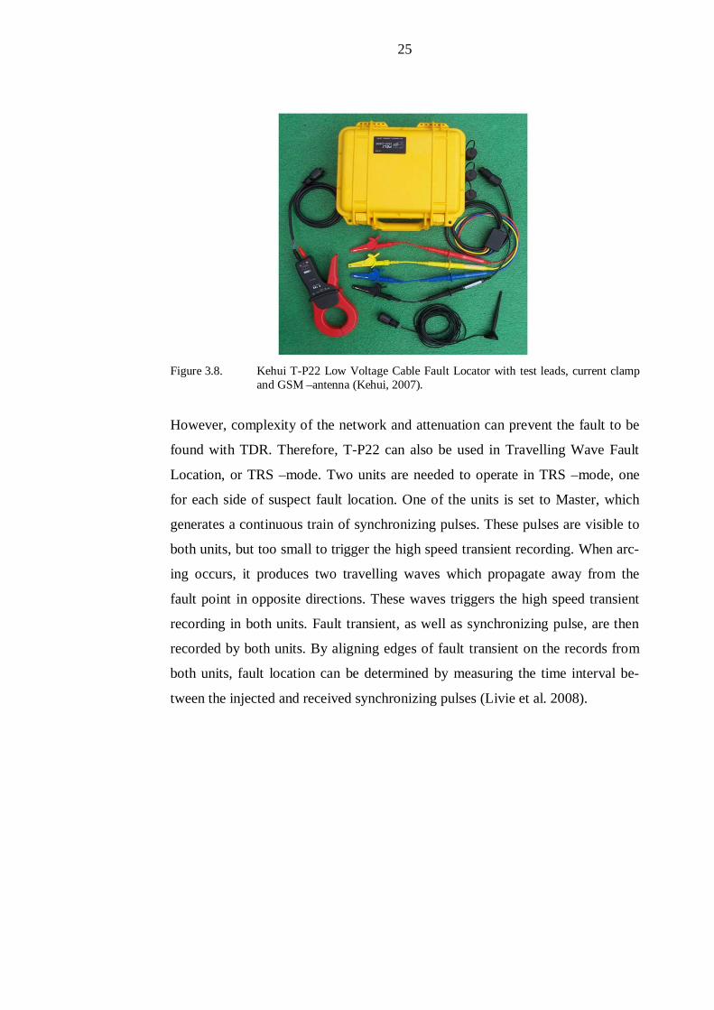
There are also commercially available on-line fault locators, designed especially
to identify and locate high impedance intermittent faults, which cause fuses to
blow occasionally. For example, Kehui T-P22 is locally or remotely operated
TDR / TRS (Transient Recording System) -device, which is connected to all 3
phases of a faulty cable. It includes a 4 channel, 3 voltages and 1 current, transi-
ent recorder. TDR system is triggered based on voltage distortion and / or over-
current. TDR trace is recorded before and during the arcing. Therefore, by com-
paring these two traces, fault location can be found in the spot where TDR trace
have changed. A picture of Kehui T-P22 is presented in Figure 3.8 (Livie et al.
2008).
25
Figure 3.8. Kehui T-P22 Low Voltage Cable Fault Locator with test leads, current clampand GSM –antenna (Kehui, 2007).
However, complexity of the network and attenuation can prevent the fault to be
found with TDR. Therefore, T-P22 can also be used in Travelling Wave Fault
Location, or TRS –mode. Two units are needed to operate in TRS –mode, one
for each side of suspect fault location. One of the units is set to Master, which
generates a continuous train of synchronizing pulses. These pulses are visible to
both units, but too small to trigger the high speed transient recording. When arc-
ing occurs, it produces two travelling waves which propagate away from the
fault point in opposite directions. These waves triggers the high speed transient
recording in both units. Fault transient, as well as synchronizing pulse, are then
recorded by both units. By aligning edges of fault transient on the records from
both units, fault location can be determined by measuring the time interval be-
tween the injected and received synchronizing pulses (Livie et al. 2008).
26
4 Condition measurements in underground cable network
Reliability demands on electricity distribution system are constantly increasing,
together with efficiency demands on DSOs operation. Therefore, precautionary
maintenance should be done as cost-efficiently as possible. Underground cable
networks form a large part of electricity distribution system, and therefore, cost-
efficient condition management of cable networks is crucial to meet constantly
increasing demands of reliability and efficiency.
Condition measurements offer information about condition of underground ca-
bles, without a need of expensive excavation work to be done. Current condition
measurement techniques are off-line methods, so the cable has to be disconnect-
ed before measurements.
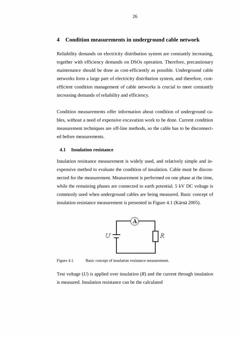
4.1 Insulation resistance
Insulation resistance measurement is widely used, and relatively simple and in-
expensive method to evaluate the condition of insulation. Cable must be discon-
nected for the measurement. Measurement is performed on one phase at the time,
while the remaining phases are connected to earth potential. 5 kV DC voltage is
commonly used when underground cables are being measured. Basic concept of
insulation resistance measurement is presented in Figure 4.1 (Kärnä 2005).
Figure 4.1. Basic concept of insulation resistance measurement.
Test voltage (U) is applied over insulation (R) and the current through insulation
is measured. Insulation resistance can be the calculated

27
= , (4.1)
where I is measured current through the insulation. Actual insulation resistance
testers calculate the insulation resistance automatically.
Resolution of insulation resistance measurement is very low; it only shows
whether the insulation is intact or not. On the other hand, low insulation re-
sistance means the insulation to be certainly seriously damaged. Insulation re-
sistance measurements are mainly used for verifying the electrical installations
and to measure the condition of windings of rotating machines (Kärnä 2005).
4.2 Dielectric loss factor
Dielectric loss factor, or tan , is measured using AC voltage. Ideal insulation
would consist only of capacitance, and it could be modeled simply using a ca-
pacitor. Practical insulation, however, includes also resistance, which allows
small resistive leakage current through the insulation. Loss angle measures the
ratio between capacitive and resistive currents as shown in Figure 4.2.
Figure 4.2. Equivalent circuit of insulation and definition of loss angle .
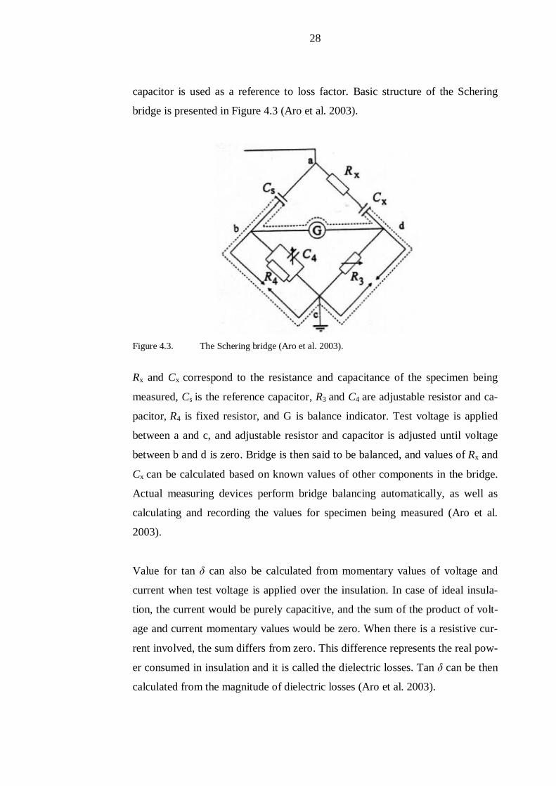
Tan and capacitance can be measured using the Schering bridge or current
comparator bridge. Bridge measurement is based on comparing the specimen
being measured to a known reference component. Compressed gas capacitor is
usually used as a reference to capacitance, and resistor connected to series with
28
capacitor is used as a reference to loss factor. Basic structure of the Schering
bridge is presented in Figure 4.3 (Aro et al. 2003).
Figure 4.3. The Schering bridge (Aro et al. 2003).
Rx and Cx correspond to the resistance and capacitance of the specimen being
measured, Cs is the reference capacitor, R3 and C4 are adjustable resistor and ca-
pacitor, R4 is fixed resistor, and G is balance indicator. Test voltage is applied
between a and c, and adjustable resistor and capacitor is adjusted until voltage
between b and d is zero. Bridge is then said to be balanced, and values of Rx and
Cx can be calculated based on known values of other components in the bridge.
Actual measuring devices perform bridge balancing automatically, as well as
calculating and recording the values for specimen being measured (Aro et al.
2003).
Value for tan can also be calculated from momentary values of voltage and
current when test voltage is applied over the insulation. In case of ideal insula-
tion, the current would be purely capacitive, and the sum of the product of volt-
age and current momentary values would be zero. When there is a resistive cur-
rent involved, the sum differs from zero. This difference represents the real pow-
er consumed in insulation and it is called the dielectric losses. Tan can be then
calculated from the magnitude of dielectric losses (Aro et al. 2003).
29
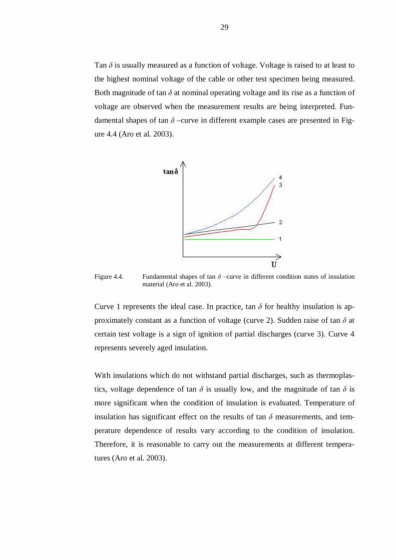
Tan is usually measured as a function of voltage. Voltage is raised to at least to
the highest nominal voltage of the cable or other test specimen being measured.
Both magnitude of tan at nominal operating voltage and its rise as a function of
voltage are observed when the measurement results are being interpreted. Fun-
damental shapes of tan –curve in different example cases are presented in Fig-
ure 4.4 (Aro et al. 2003).
Figure 4.4. Fundamental shapes of tan –curve in different condition states of insulationmaterial (Aro et al. 2003).
Curve 1 represents the ideal case. In practice, tan for healthy insulation is ap-
proximately constant as a function of voltage (curve 2). Sudden raise of tan at
certain test voltage is a sign of ignition of partial discharges (curve 3). Curve 4
represents severely aged insulation.
With insulations which do not withstand partial discharges, such as thermoplas-
tics, voltage dependence of tan is usually low, and the magnitude of tan is
more significant when the condition of insulation is evaluated. Temperature of
insulation has significant effect on the results of tan measurements, and tem-
perature dependence of results vary according to the condition of insulation.
Therefore, it is reasonable to carry out the measurements at different tempera-
tures (Aro et al. 2003).
30
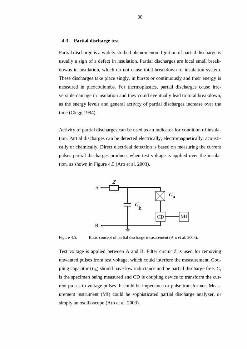
4.3 Partial discharge test
Partial discharge is a widely studied phenomenon. Ignition of partial discharge is
usually a sign of a defect in insulation. Partial discharges are local small break-
downs in insulation, which do not cause total breakdown of insulation system.
These discharges take place singly, in bursts or continuously and their energy is
measured in picocoulombs. For thermoplastics, partial discharges cause irre-
versible damage in insulation and they could eventually lead to total breakdown,
as the energy levels and general activity of partial discharges increase over the
time (Clegg 1994).
Activity of partial discharges can be used as an indicator for condition of insula-
tion. Partial discharges can be detected electrically, electromagnetically, acousti-
cally or chemically. Direct electrical detection is based on measuring the current
pulses partial discharges produce, when test voltage is applied over the insula-
tion, as shown in Figure 4.5 (Aro et al. 2003).
Figure 4.5. Basic concept of partial discharge measurement (Aro et al. 2003).
Test voltage is applied between A and B. Filter circuit Z is used for removing
unwanted pulses from test voltage, which could interfere the measurement. Cou-
pling capacitor (Ck) should have low inductance and be partial discharge free. Ca
is the specimen being measured and CD is coupling device to transform the cur-
rent pulses to voltage pulses. It could be impedance or pulse transformer. Meas-
urement instrument (MI) could be sophisticated partial discharge analyzer, or
simply an oscilloscope (Aro et al. 2003).

31
For MV and HV cables, novel condition monitoring techniques, based on detec-
tion of partial discharges, have been developed to be used on-line. Sensitive par-
tial discharge (PD) sensor is either inductively or capacitively coupled to dielec-
tric. The sensor could be, for example, high frequency current transformer
around the lead from concentric conductor to earth. The signal from PD sensor is
then passed through high-pass filter and several broadband amplifiers in cascade.
Filtered and amplified signal is then digitalized and transferred to PC for analy-
sis. In real installation environments, noise, attenuation and distortion of PD sig-
nals cause challenges for on-line PD measurement (Blackburn et al. 2005).
4.4 Differences between MV and LV networks
The main difference between LV and MV networks from condition measure-
ments point of view is higher voltage stress in MV cables. Higher voltage stress
causes fault propagation to be faster and more straightforward than in LV ca-
bles. Any defect or void in cable insulation will initiate PDs in MV cables as the
strength of electric field over the void exceeds the breakdown strength of air.
PDs occur also in damaged LV cables, but it requires serious damage in the ca-
ble, presence of moisture and leakage current. PD activity is also more random in
damaged LV cables than in damaged MV cables. PD activity level can therefore
be used for measuring the condition of a MV cable, but cannot be reliably used
for evaluating the condition of a LV cable as the PD activity in LV cable usually
means that the cable is already very severely damaged.
Topology of MV cable feeder differs from topology of LV cable feeder. A single
MV cable usually runs between two secondary substations, connecting them to-
gether. Both substations are also usually equipped with disconnectors, allowing
the cable to be disconnected for service or for off-line measurements. MV net-
works are usually built interconnected, so a single MV cable can often be dis-
connected without causing an outage. Exception for that is some rural under-
ground MV networks where overhead lines are replaced with underground ca-
bles and very simple network structure and satellite secondary substations are

32
used without any interconnections. However, also the cost from an interruption is
much lower in those areas than in densely populated areas.
LV cable feeder consists of the main line and branches and customer connection
cables connected to the main line. Branches can be connected through fuses in
distribution cabinets, or directly without fuses in smaller cabinets or in vertical
plastic tubes located under the ground. In densely populated urban areas, there
are usually some interconnections between different LV networks. Overall, to-
pology of LV network is more complex than MV network which makes fault
location and condition measurements more challenging.
33
5 Novel on-line condition monitoring methods
This thesis included planning and executing laboratory measurements to study
usability of high frequency signal injection techniques in condition monitoring of
underground LV cables. Measurement setup and execution will be described
briefly in this Chapter with the most important results. Theoretical approach and
more detailed analysis of the measurements and results can be found from mas-
ter’s thesis “Channel Estimation and On-line Diagnosis of LV Distribution Ca-
bling”. Ideas and possible challenges regarding to the practical implementation
of OCM to the LV networks are also presented in this Chapter.
5.1 Laboratory measurements
Objective of measurements was to determine whether it is possible to detect con-
sistent change in high frequency signal response before an electrical fault devel-
ops when cable is damaged under wet conditions. Moisture alters characteristic
impedance of the cable and therefore, it increases attenuation and it causes re-
flections.
General definition of high frequency band is a frequency range from 3 MHz to
30 MHz, however, in this thesis, the whole measurement range from 100 kHz to
100 MHz is referred as high frequency. Cable electrical condition was evaluated
by insulation resistance measurements and by applying line voltage to the dam-
aged cable.
5.1.1 Test setup
Two most commonly used modern LV cables in Finish distribution networks
were selected; PVC insulated AMCMK and XLPE insulated AXMK. Properties
of these cables are presented in Table 2.1.
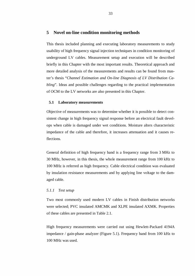
High frequency measurements were carried out using Hewlett-Packard 4194A
impedance / gain-phase analyzer (Figure 5.1). Frequency band from 100 kHz to
100 MHz was used.
34
Figure 5.1. Hewlett-Packard 4194A impedance / gain-phase analyzer.
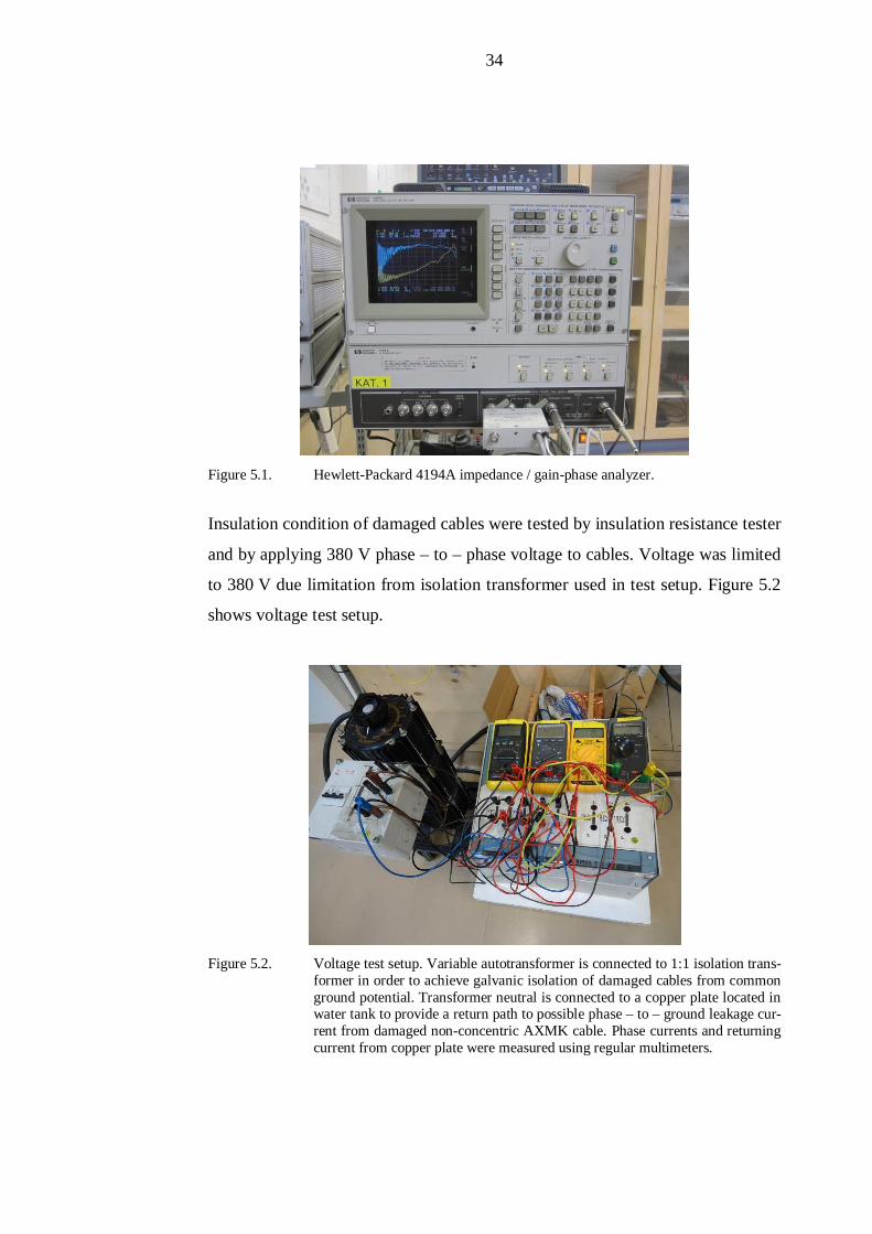
Insulation condition of damaged cables were tested by insulation resistance tester
and by applying 380 V phase – to – phase voltage to cables. Voltage was limited
to 380 V due limitation from isolation transformer used in test setup. Figure 5.2
shows voltage test setup.
Figure 5.2. Voltage test setup. Variable autotransformer is connected to 1:1 isolation trans-former in order to achieve galvanic isolation of damaged cables from commonground potential. Transformer neutral is connected to a copper plate located inwater tank to provide a return path to possible phase – to – ground leakage cur-rent from damaged non-concentric AXMK cable. Phase currents and returningcurrent from copper plate were measured using regular multimeters.

35
Two different test setups were built for single cable segments. In both cases,
damaged part of the cables were submerged under regular tap water. Properties
of tap water would not fully correspond with the properties of moisture in the
soil, but it was used in order to maintain as controlled test environment as possi-
ble. However, lack of salt and other impurities cause the tap water to be less
conductive than average soil moisture, which could affect especially to the leak-
age current measurements.
5.1.2 Long term water test
Tests were divided in two different categories, long-term water test and progres-
sive damaging. Long-term water test were carried out with 25 m long samples of
both cable types. A 10 cm long section of outer sheath and the polypropylene
bands were cut away from both cables. Damage was done at 11 m from closest
cable end. Insulation around the phase conductors were left intact. After the ca-
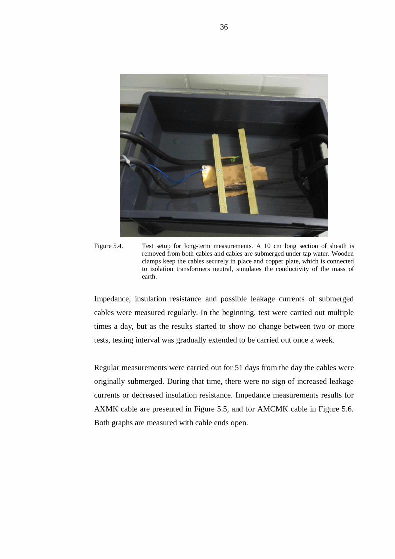
bles were measured dry, they were submerged under water. Figure 5.3 shows
AMCMK –cable with section of sheath removed and Figure 5.4 shows sub-
merged cables during the long-term water test.
Figure 5.3. AMCMK cable with 10 cm long section of sheath and polypropylene tapesremoved.
36
Figure 5.4. Test setup for long-term measurements. A 10 cm long section of sheath isremoved from both cables and cables are submerged under tap water. Woodenclamps keep the cables securely in place and copper plate, which is connectedto isolation transformers neutral, simulates the conductivity of the mass ofearth.
Impedance, insulation resistance and possible leakage currents of submerged
cables were measured regularly. In the beginning, test were carried out multiple
times a day, but as the results started to show no change between two or more
tests, testing interval was gradually extended to be carried out once a week.
Regular measurements were carried out for 51 days from the day the cables were
originally submerged. During that time, there were no sign of increased leakage
currents or decreased insulation resistance. Impedance measurements results for
AXMK cable are presented in Figure 5.5, and for AMCMK cable in Figure 5.6.
Both graphs are measured with cable ends open.
37
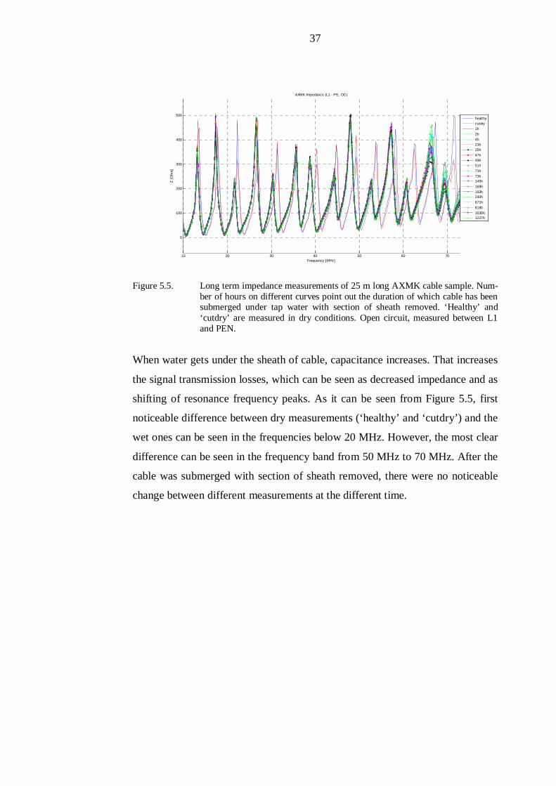
Figure 5.5. Long term impedance measurements of 25 m long AXMK cable sample. Num-ber of hours on different curves point out the duration of which cable has beensubmerged under tap water with section of sheath removed. ‘Healthy’ and‘cutdry’ are measured in dry conditions. Open circuit, measured between L1and PEN.
When water gets under the sheath of cable, capacitance increases. That increases
the signal transmission losses, which can be seen as decreased impedance and as
shifting of resonance frequency peaks. As it can be seen from Figure 5.5, first
noticeable difference between dry measurements (‘healthy’ and ‘cutdry’) and the
wet ones can be seen in the frequencies below 20 MHz. However, the most clear
difference can be seen in the frequency band from 50 MHz to 70 MHz. After the
cable was submerged with section of sheath removed, there were no noticeable
change between different measurements at the different time.
10 20 30 40 50 60 70
0
100
200
300
400
500
Frequency [MHz]
Z [O
hm]
AXMK Impedance (L1 - PE, OC)
healthycutdry1h2h4h23h25h47h49h51h71h73h145h169h193h240h671h818h1035h1227h

38
Figure 5.6. Long term impedance measurements of 25 m AMCMK cable sample. Numberof hours on different curves point out the duration of which cable has beensubmerged under tap water with section of sheath removed. ‘Healthy’ and‘cutdry’ are measured in dry conditions. Open circuit, measured between L1and PEN.
Difference between dry and wet cables is not as clear with AMCMK as it is with
AXMK (Figure 5.5). This is due higher attenuation of PVC, compared to the
XLPE. Thus, AXMK or other XLPE insulated cables are more suitable for high
frequency signal injection –based condition monitoring than the PVC insulated
AMCMK. There are some differences between different wet measurements in
the frequency band from 50 MHz to 70 MHz (Figure 5.7).
10 20 30 40 50 60 700
50
100
150
200
Frequency [MHz]
Z [O
hm]
AMCMK Impedance (L1 - PE, OC)
healthycutdry1h2h4h23h25h47h49h51h71h73h145h169h193h240h671h818h1035h1227h
39
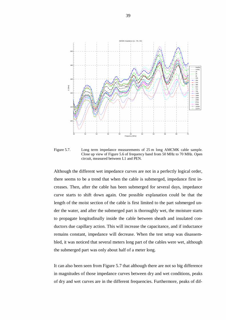
Figure 5.7. Long term impedance measurements of 25 m long AMCMK cable sample.Close up view of Figure 5.6 of frequency band from 50 MHz to 70 MHz. Opencircuit, measured between L1 and PEN.
Although the different wet impedance curves are not in a perfectly logical order,
there seems to be a trend that when the cable is submerged, impedance first in-
creases. Then, after the cable has been submerged for several days, impedance
curve starts to shift down again. One possible explanation could be that the
length of the moist section of the cable is first limited to the part submerged un-
der the water, and after the submerged part is thoroughly wet, the moisture starts
to propagate longitudinally inside the cable between sheath and insulated con-
ductors due capillary action. This will increase the capacitance, and if inductance
remains constant, impedance will decrease. When the test setup was disassem-
bled, it was noticed that several meters long part of the cables were wet, although
the submerged part was only about half of a meter long.
It can also been seen from Figure 5.7 that although there are not so big difference
in magnitudes of those impedance curves between dry and wet conditions, peaks
of dry and wet curves are in the different frequencies. Furthermore, peaks of dif-
50 52 54 56 58 60 62 64 66 68 70
100
120
140
160
180
200
Frequency [MHz]
Z [O
hm]
AMCMK Impedance (L1 - PE, OC)
healthycutdry1h2h4h23h25h47h49h51h71h73h145h169h193h240h671h818h1035h1227h
40
ferent wet measurements are in the same frequency, despite that there is some
variation in magnitudes between different measurements.
5.1.3 Progressive damaging of insulation
Progressive damaging was done to two 50 m long samples of both cables. Part of
sheath was removed similar way as in the long term measurements (Figure 5.3).
Damage was done to 17 m from the closest cable end, which corresponds about
one third of cable length. Similar water tank and copper plate setup was used as
with the long term measurements (Figure 5.4). After mechanical damage to insu-
lation was done, cables were submerged and left under the water for at least for
24 h. Cables were measured multiple times during that period.
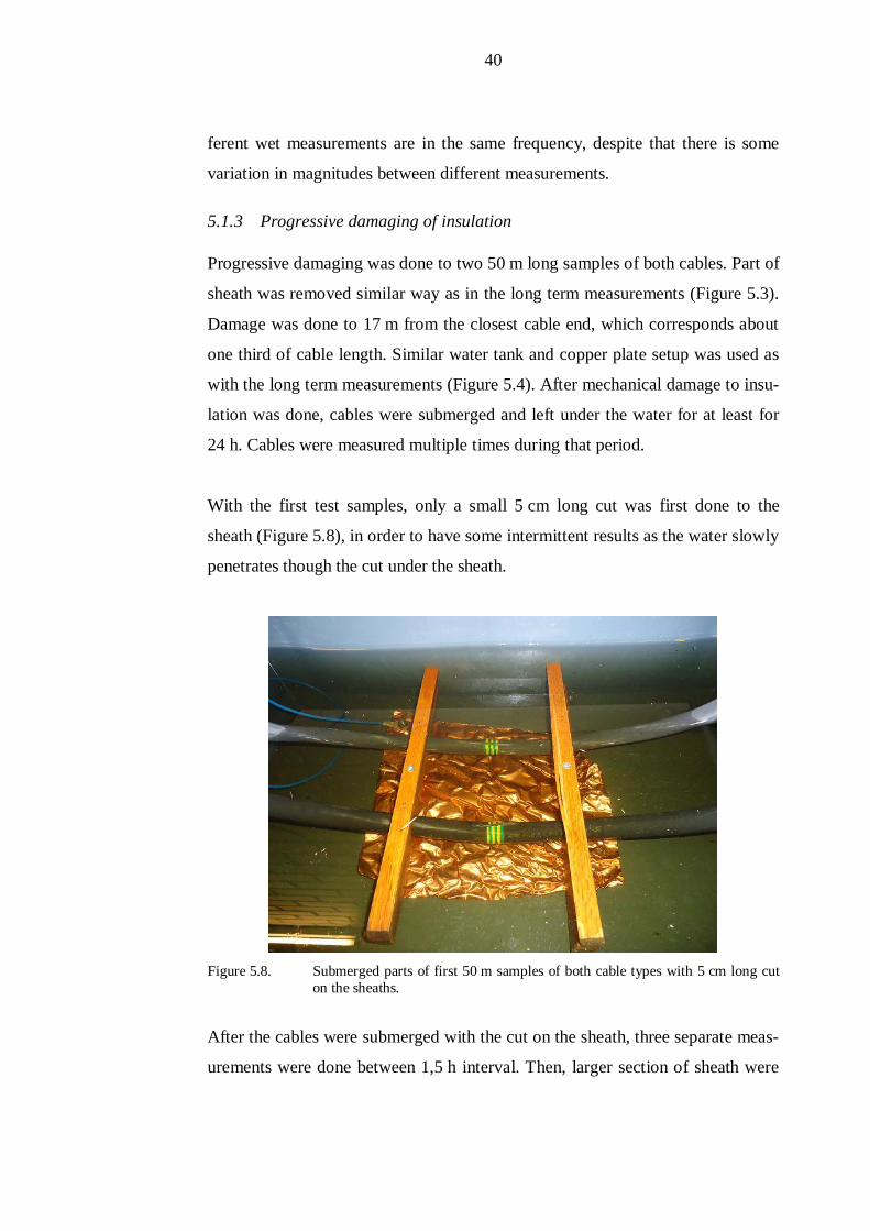
With the first test samples, only a small 5 cm long cut was first done to the
sheath (Figure 5.8), in order to have some intermittent results as the water slowly
penetrates though the cut under the sheath.
Figure 5.8. Submerged parts of first 50 m samples of both cable types with 5 cm long cuton the sheaths.
After the cables were submerged with the cut on the sheath, three separate meas-
urements were done between 1,5 h interval. Then, larger section of sheath were
41
cut away, and the damaging process of insulation was started. Only phase one
(brown) insulation was damaged with the first 50 m samples. Insulation thick-
ness was gradually decreased in three steps, until at the final step 30 x 3 mm area
of bare aluminum conductor was exposed. First degree damage to AMCMK is
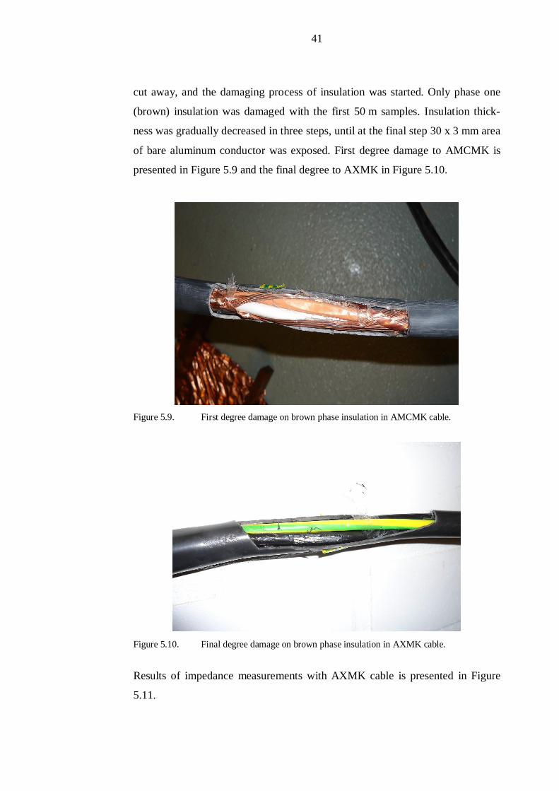
presented in Figure 5.9 and the final degree to AXMK in Figure 5.10.
Figure 5.9. First degree damage on brown phase insulation in AMCMK cable.
Figure 5.10. Final degree damage on brown phase insulation in AXMK cable.
Results of impedance measurements with AXMK cable is presented in Figure
5.11.
42
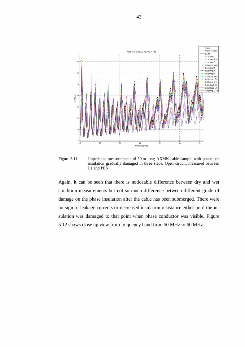
Figure 5.11. Impedance measurements of 50 m long AXMK cable sample with phase oneinsulation gradually damaged in three steps. Open circuit, measured betweenL1 and PEN.
Again, it can be seen that there is noticeable difference between dry and wet
condition measurements but not so much difference between different grade of
damage on the phase insulation after the cable has been submerged. There were
no sign of leakage currents or decreased insulation resistance either until the in-
sulation was damaged to that point when phase conductor was visible. Figure
5.12 shows close up view from frequency band from 50 MHz to 60 MHz.
10 20 30 40 50 60 700
50
100
150
200
250
300
350
Frequency [MHz]
Z [O
hm]
AXMK Impedance (L1 - PE, OC) 0 -> 50
healthyhealthy in watercut drycut in watercut in water 1 5hcut in water 3hsheatcut in water1stdgrdmg 1h1stdgrdmg 2h1stdgrdmg25h2nddgrdmg 0 5 h2nddgrdmg 2 5 h2nddgrdmg 69 h3rddgrdmg 0 5 h3rddgrdmg 2 5 h3rddgrdmg 21 5 h

43
Figure 5.12. Impedance measurement results of progressive damaging of 50 m long AXMKcable sample. Close up view of Figure 5.11 of frequency band from 50 MHz to60 MHz. Open circuit, measured between L1 and PEN.
Some difference at certain frequencies can be noticed between those measure-
ments where only a small cut was made on the sheath and cable was submerged
(‘cut in water’) and the rest of wet measurements. However, there is practically
no change in three different measurements made between 1,5 h interval, so the
submerged part of the cable was most probably already wet during the first set of
measurements. Possible explanation for the difference between those and the rest
of the wet measurements, with larger section of sheath removed, could be that
the polypropylene taping was not damaged when the smaller cut was made.
Therefore, the water could not get between the phase conductors, only between
sheath and polypropylene taping. No noticeable change in impedance between
different damage grades.
Second cable samples were damaged similar way, but two phases were damaged
instead of one. This will cause the voltage stress over damaged insulations to be
higher. With the non-concentric AXMK cable, also the resistance between two
50 51 52 53 54 55 56 57 58 590
50
100
150
200
250
300
350
Frequency [MHz]
Z [O
hm]
AXMK Impedance (L1 - PE, OC) 0 -> 50
healthyhealthy in watercut drycut in watercut in water 1 5hcut in water 3hsheatcut in water1stdgrdmg 1h1stdgrdmg 2h1stdgrdmg25h2nddgrdmg 0 5 h2nddgrdmg 2 5 h2nddgrdmg 69 h3rddgrdmg 0 5 h3rddgrdmg 2 5 h3rddgrdmg 21 5 h
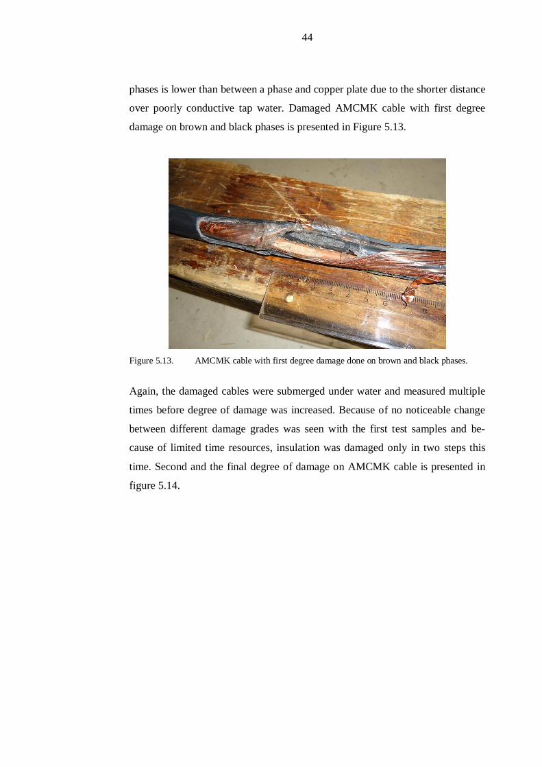
44
phases is lower than between a phase and copper plate due to the shorter distance
over poorly conductive tap water. Damaged AMCMK cable with first degree
damage on brown and black phases is presented in Figure 5.13.
Figure 5.13. AMCMK cable with first degree damage done on brown and black phases.
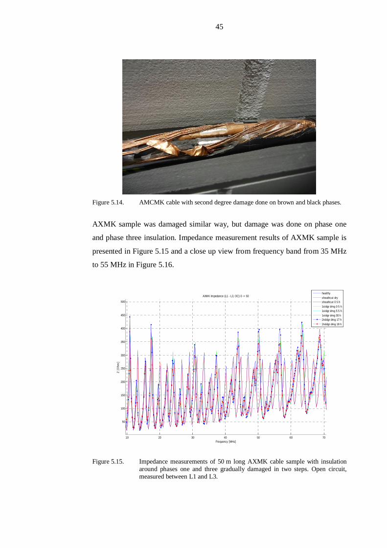
Again, the damaged cables were submerged under water and measured multiple
times before degree of damage was increased. Because of no noticeable change
between different damage grades was seen with the first test samples and be-
cause of limited time resources, insulation was damaged only in two steps this
time. Second and the final degree of damage on AMCMK cable is presented in
figure 5.14.
45
Figure 5.14. AMCMK cable with second degree damage done on brown and black phases.
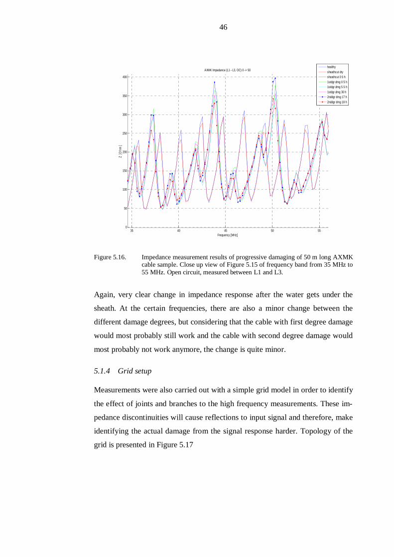
AXMK sample was damaged similar way, but damage was done on phase one
and phase three insulation. Impedance measurement results of AXMK sample is
presented in Figure 5.15 and a close up view from frequency band from 35 MHz
to 55 MHz in Figure 5.16.
Figure 5.15. Impedance measurements of 50 m long AXMK cable sample with insulationaround phases one and three gradually damaged in two steps. Open circuit,measured between L1 and L3.
10 20 30 40 50 60 70
50
100
150
200
250
300
350
400
450
500
Frequency [MHz]
Z [O
hm]
AXMK Impedance (L1 - L3, OC) 0 -> 50healthysheathcut drysheathcut 0 5 h1stdgr dmg 0 5 h1stdgr dmg 5 5 h1stdgr dmg 30 h2nddgr dmg 17 h2nddgr dmg 18 h
46
Figure 5.16. Impedance measurement results of progressive damaging of 50 m long AXMKcable sample. Close up view of Figure 5.15 of frequency band from 35 MHz to55 MHz. Open circuit, measured between L1 and L3.
Again, very clear change in impedance response after the water gets under the
sheath. At the certain frequencies, there are also a minor change between the
different damage degrees, but considering that the cable with first degree damage
would most probably still work and the cable with second degree damage would
most probably not work anymore, the change is quite minor.
5.1.4 Grid setup
Measurements were also carried out with a simple grid model in order to identify
the effect of joints and branches to the high frequency measurements. These im-
pedance discontinuities will cause reflections to input signal and therefore, make
identifying the actual damage from the signal response harder. Topology of the
grid is presented in Figure 5.17
35 40 45 50 550
50
100
150
200
250
300
350
400
Frequency [MHz]
Z [O
hm]
AXMK Impedance (L1 - L3, OC) 0 -> 50healthysheathcut drysheathcut 0 5 h1stdgr dmg 0 5 h1stdgr dmg 5 5 h1stdgr dmg 30 h2nddgr dmg 17 h2nddgr dmg 18 h
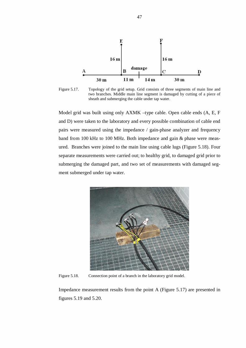
47
Figure 5.17. Topology of the grid setup. Grid consists of three segments of main line andtwo branches. Middle main line segment is damaged by cutting of a piece ofsheath and submerging the cable under tap water.
Model grid was built using only AXMK –type cable. Open cable ends (A, E, F
and D) were taken to the laboratory and every possible combination of cable end
pairs were measured using the impedance / gain-phase analyzer and frequency
band from 100 kHz to 100 MHz. Both impedance and gain & phase were meas-
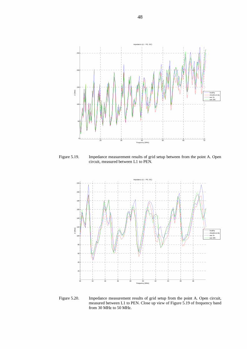
ured. Branches were joined to the main line using cable lugs (Figure 5.18). Four
separate measurements were carried out; to healthy grid, to damaged grid prior to
submerging the damaged part, and two set of measurements with damaged seg-
ment submerged under tap water.
Figure 5.18. Connection point of a branch in the laboratory grid model.
Impedance measurement results from the point A (Figure 5.17) are presented in
figures 5.19 and 5.20.
48
Figure 5.19. Impedance measurement results of grid setup between from the point A. Opencircuit, measured between L1 to PEN.
Figure 5.20. Impedance measurement results of grid setup from the point A. Open circuit,measured between L1 to PEN. Close up view of Figure 5.19 of frequency bandfrom 30 MHz to 50 MHz.
20 30 40 50 60 700
50
100
150
200
250
Frequency [MHz]
Z [O
hm]
Impedance (L1 - PE, OC)
healthysheathcut drywet 1hwet 20h
30 32 34 36 38 40 42 44 46 48
20
40
60
80
100
120
140
160
180
200
220
Frequency [MHz]
Z [O
hm]
Impedance (L1 - PE, OC)
healthysheathcut drywet 1hwet 20h

49
It can be seen that there is again noticeable differences in impedance measure-
ments between dry and wet measurements, although there are more noise due
reflections from the branches and joints. In figure 5.21, results from gain &
phase measurements from A to D (Figure 5.17) are presented in distance domain.
Conversion from frequency domain through time domain to distance domain is
done by inverse Fourier transform and by assuming a certain propagation speed
to the measurement signal (Hernandez, 2012).
Figure 5.21. Results from gain & phase measurements from the grid point A to the point Dpresented in distance domain. Measured between L1 and L3 with the end of thebranches being open. A value of 0,72 · c was used for signal propagation speed(Hernandez, 2012).
Markings in the Figure 5.21 are related to the Figure 5.17. As it can been seen,
reflections from the open ends of branches, from the joints, and from the dam-
aged part of the cable could be identified and located. Length of the connection
cables, about 3 m in total, between analyzer and the grid setup should be taken in
account when comparing figure 5.21 to the topology of the grid setup. Error in
the distance will grow as the distance grows because of the error in the meas-
urement signal propagation speed assumption will accumulate. Signal propaga-
tion speed also decreases when the signal passes through the damaged part due to
higher capacitance.
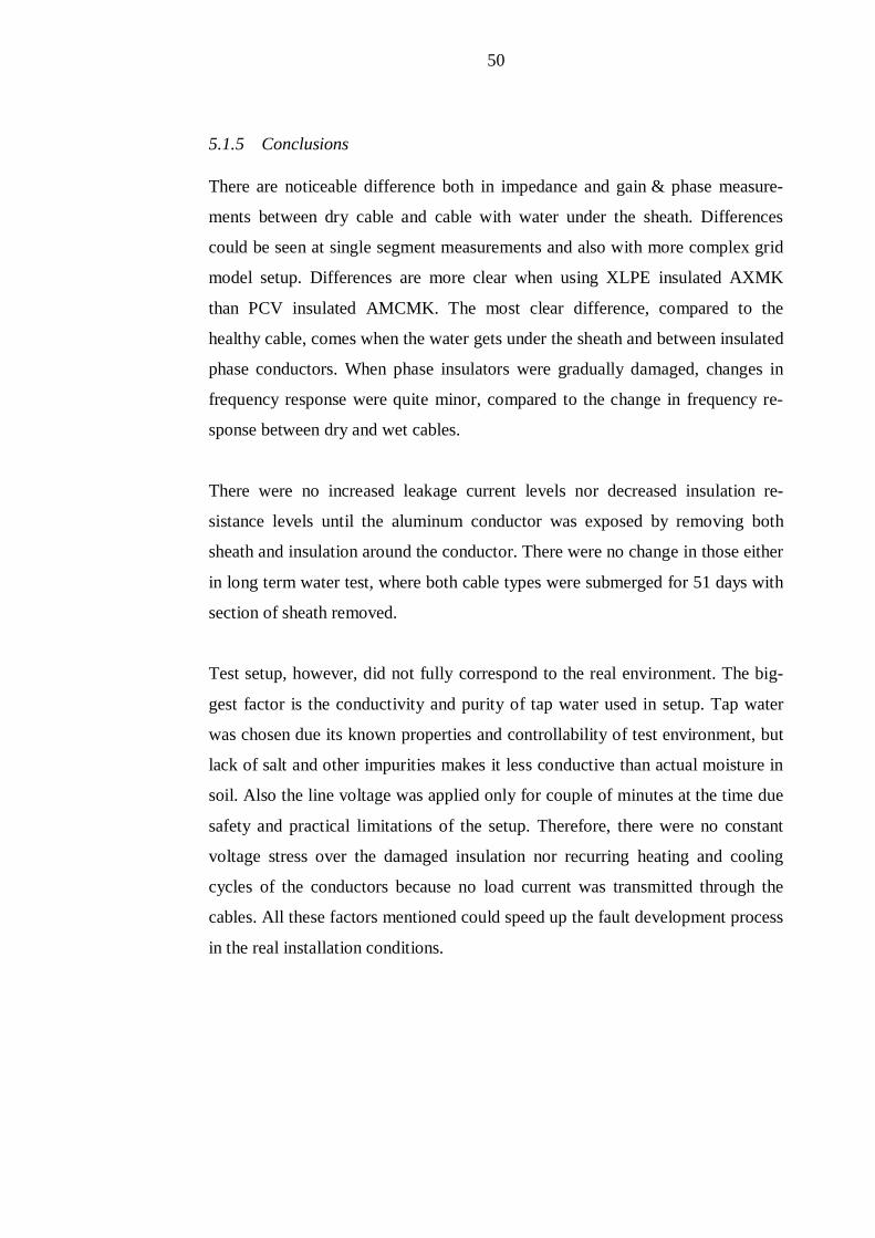
50
5.1.5 Conclusions
There are noticeable difference both in impedance and gain & phase measure-
ments between dry cable and cable with water under the sheath. Differences
could be seen at single segment measurements and also with more complex grid
model setup. Differences are more clear when using XLPE insulated AXMK
than PCV insulated AMCMK. The most clear difference, compared to the
healthy cable, comes when the water gets under the sheath and between insulated
phase conductors. When phase insulators were gradually damaged, changes in
frequency response were quite minor, compared to the change in frequency re-
sponse between dry and wet cables.
There were no increased leakage current levels nor decreased insulation re-
sistance levels until the aluminum conductor was exposed by removing both
sheath and insulation around the conductor. There were no change in those either
in long term water test, where both cable types were submerged for 51 days with
section of sheath removed.
Test setup, however, did not fully correspond to the real environment. The big-
gest factor is the conductivity and purity of tap water used in setup. Tap water
was chosen due its known properties and controllability of test environment, but
lack of salt and other impurities makes it less conductive than actual moisture in
soil. Also the line voltage was applied only for couple of minutes at the time due
safety and practical limitations of the setup. Therefore, there were no constant
voltage stress over the damaged insulation nor recurring heating and cooling
cycles of the conductors because no load current was transmitted through the
cables. All these factors mentioned could speed up the fault development process
in the real installation conditions.
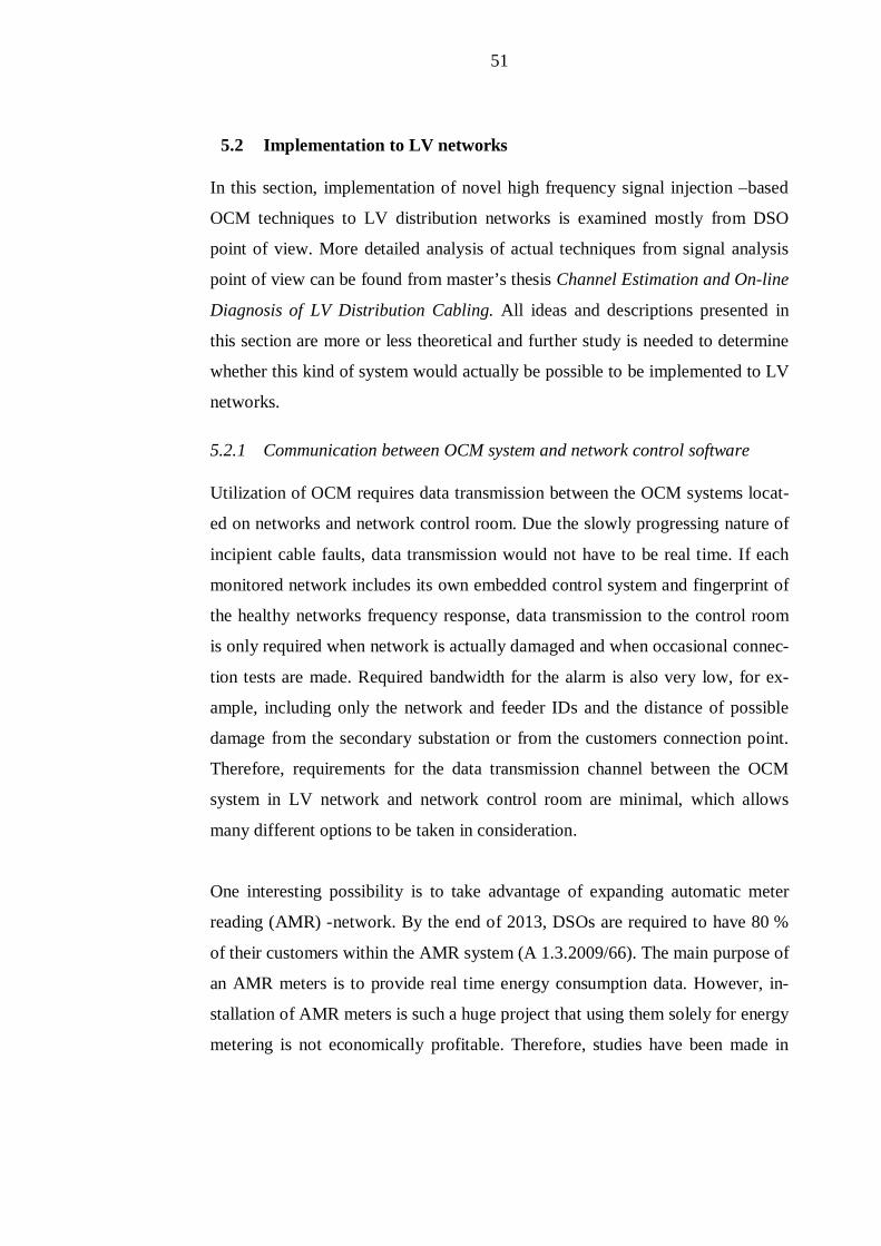
51
5.2 Implementation to LV networks
In this section, implementation of novel high frequency signal injection –based
OCM techniques to LV distribution networks is examined mostly from DSO
point of view. More detailed analysis of actual techniques from signal analysis
point of view can be found from master’s thesis Channel Estimation and On-line
Diagnosis of LV Distribution Cabling. All ideas and descriptions presented in
this section are more or less theoretical and further study is needed to determine
whether this kind of system would actually be possible to be implemented to LV
networks.
5.2.1 Communication between OCM system and network control software
Utilization of OCM requires data transmission between the OCM systems locat-
ed on networks and network control room. Due the slowly progressing nature of
incipient cable faults, data transmission would not have to be real time. If each
monitored network includes its own embedded control system and fingerprint of
the healthy networks frequency response, data transmission to the control room
is only required when network is actually damaged and when occasional connec-
tion tests are made. Required bandwidth for the alarm is also very low, for ex-
ample, including only the network and feeder IDs and the distance of possible
damage from the secondary substation or from the customers connection point.
Therefore, requirements for the data transmission channel between the OCM
system in LV network and network control room are minimal, which allows
many different options to be taken in consideration.
One interesting possibility is to take advantage of expanding automatic meter
reading (AMR) -network. By the end of 2013, DSOs are required to have 80 %
of their customers within the AMR system (A 1.3.2009/66). The main purpose of
an AMR meters is to provide real time energy consumption data. However, in-
stallation of AMR meters is such a huge project that using them solely for energy
metering is not economically profitable. Therefore, studies have been made in
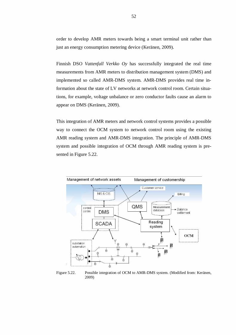
52
order to develop AMR meters towards being a smart terminal unit rather than
just an energy consumption metering device (Keränen, 2009).
Finnish DSO Vattenfall Verkko Oy has successfully integrated the real time
measurements from AMR meters to distribution management system (DMS) and
implemented so called AMR-DMS system. AMR-DMS provides real time in-
formation about the state of LV networks at network control room. Certain situa-
tions, for example, voltage unbalance or zero conductor faults cause an alarm to
appear on DMS (Keränen, 2009).
This integration of AMR meters and network control systems provides a possible
way to connect the OCM system to network control room using the existing
AMR reading system and AMR-DMS integration. The principle of AMR-DMS
system and possible integration of OCM through AMR reading system is pre-
sented in Figure 5.22.
Figure 5.22. Possible integration of OCM to AMR-DMS system. (Modified from: Keränen,2009)
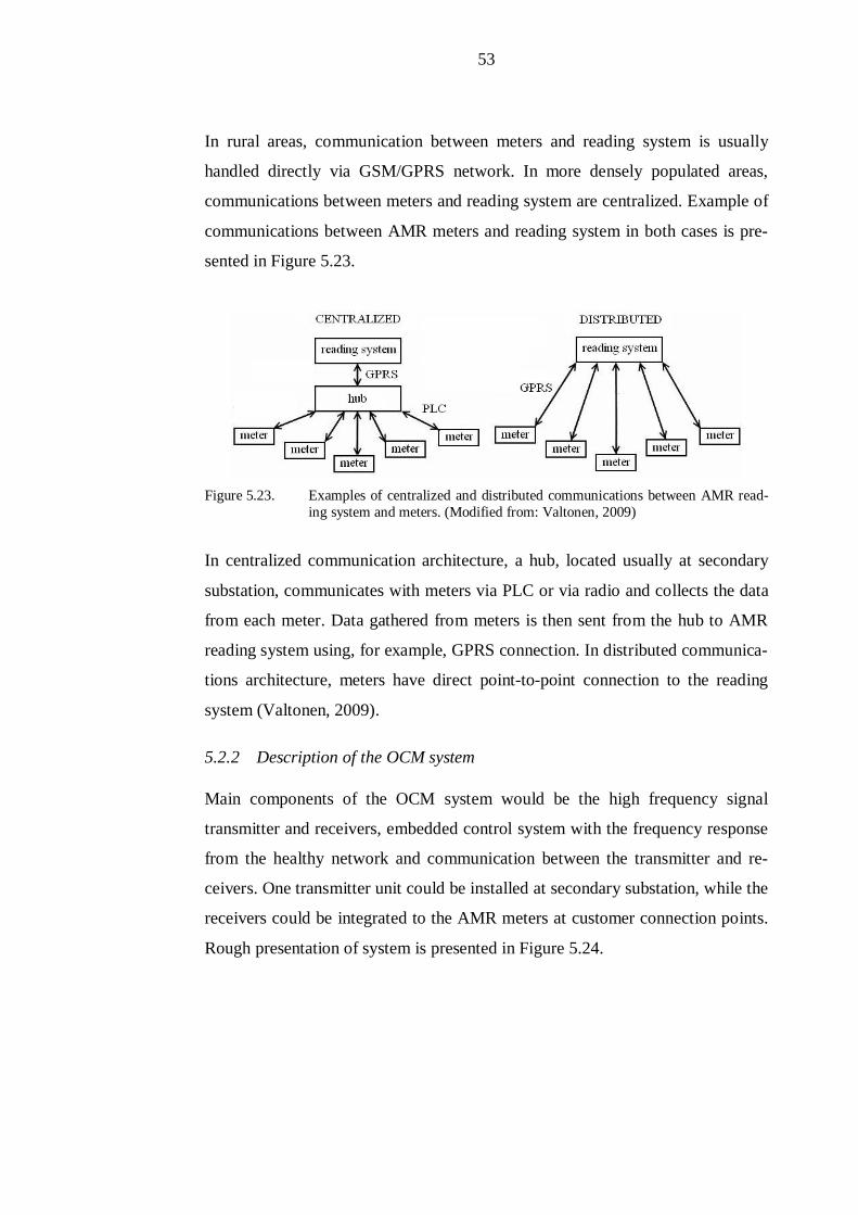
53
In rural areas, communication between meters and reading system is usually
handled directly via GSM/GPRS network. In more densely populated areas,
communications between meters and reading system are centralized. Example of
communications between AMR meters and reading system in both cases is pre-
sented in Figure 5.23.
Figure 5.23. Examples of centralized and distributed communications between AMR read-ing system and meters. (Modified from: Valtonen, 2009)
In centralized communication architecture, a hub, located usually at secondary
substation, communicates with meters via PLC or via radio and collects the data
from each meter. Data gathered from meters is then sent from the hub to AMR
reading system using, for example, GPRS connection. In distributed communica-
tions architecture, meters have direct point-to-point connection to the reading
system (Valtonen, 2009).
5.2.2 Description of the OCM system
Main components of the OCM system would be the high frequency signal
transmitter and receivers, embedded control system with the frequency response
from the healthy network and communication between the transmitter and re-
ceivers. One transmitter unit could be installed at secondary substation, while the
receivers could be integrated to the AMR meters at customer connection points.
Rough presentation of system is presented in Figure 5.24.

54
Figure 5.24. OCM system implemented to LV network with centralized read AMR meters.
Control system at substation uses the high frequency signal transmitter to trans-
mit a high frequency sweep to the network at specified time interval. This inter-
val could be, for example, once a day. Receiver units at customer connection
points then receive that signal and store it temporarily to memory. Next, receiver
units take advance of the AMR meters by sending received signal back to sec-
ondary substation using the communication between meters and the AMR hub.
Control system reads the received signals and compares them to the previously
stored fingerprint from healthy network. If comparison shows constant change in
response, which exceeds the preset boundaries for multiple subsequent meas-
urements, it changes the state from healthy to damaged. Next time the AMR me-
ters are being read in that LV network, declaration of possible damaged cable
reach the DMS though AMR reading system.
The first problem is to get the frequency response fingerprint from a certainly
healthy network. If it is measured, then usability of this OCM system is limited
only to new, certainly healthy LV networks. Even then, if a cable is damaged
during installation and it is already wet when the fingerprint is being measured,
system would not work properly. Also loads and nonlinear power supplies can
cause problems to measurements. An ideal case would be that the fingerprint
could be simulated by knowing the exact lengths and types of cables and joints
used. Problem with the simulation is to get the models accurate enough to corre-
spond with the real networks.
55
Second serious challenge to be solved is to determine the correct time to repair
or replace a cable which is reported to have moisture under the sheath by OCM.
Only conclusion from laboratory measurements, regarding to the lifetime of wet
thermoplastic insulated LV cables, was that they survive at least two months
with sheath partially removed under regular tap water. In order to determine the
time it takes from that point when sheath is damaged and the moisture gets under
the sheath, to the point when cable is no longer capable of carrying power, some
real long-term tests are needed to be done in real installation environments with
constantly energized cables carrying varying load currents. That kind of experi-
ment, however, would take a lot of time and a lot of different cables in different
installation conditions before anything conclusive results could be obtained.
According to the laboratory measurements, first noticeable changes in frequency
response between healthy and wet cables could be seen at frequencies above
20 MHz, while the most clear results were usually between 40 - 60 MHz. Using
such high frequencies, also signal attenuation causes problems and it sets a limit
to the longest possible distance between transmitter and receiver units. Higher
frequency causes more attenuation and shortens the maximum usable distance.
For example, when using 30 MHz frequency, maximum distance for PVC insu-
lated AMCMK would be 100 - 200 m. (Ahola, 2012)
Because customers are constantly changing the amount of load in the network,
also the impedance seen from the network changes. This could cause problems to
the measurements and therefore, measurements should be carried out during a
night when variation of loads is at the lowest. There are still some base loads
switching on and off though, such as heating appliances and refrigerators.
Measurement signal gets reflected from every impedance discontinuities, such as
joints and open cable ends. Therefore, customer internal networks could cause
problems to measurements due numerous reflections back to the distribution
network direction. At densely populated urban areas, one secondary substation
could have over ten different LV feeders. If the measurement signal is transmit-
56
ted to the every feeder simultaneously, reflections from numerous branches at
different feeders could also cause problems.
In order to prevent the reflections from customer internal networks and from
different LV feeders, some signal filtering is needed. Filtering can be done either
with hardware -based low pass –filters, or possibly, with software algorithms.
The main problem with hardware filters is extra costs and increased power loss-
es. One LV network can consist of over ten feeders and tens of customer connec-
tion points. Thus, cost from filters could easily increase the total implementation
costs of OCM system per LV network, even though the cost of one filter is rela-
tively low. According to source, pulse from TDR device can be filtered with
simple series inductance, made from several turns of heavy duty flexible connec-
tion cable (Clegg, 1993 p.223). This would be very cheap solution, and if the
cross section of the cable in the filter coil would be large enough, practically no
extra losses are caused.
The main problem is physical size and placement of such coils. Filter coils must
be connected in series between feeders and busbars at secondary substation and
between AMR meter and customer internal network at customer side, i.e. so that
communication between transmitter and receiver units and between AMR meters
and AMR hub are not blocked. Thickness of the wire in customer side coils,
however, could be much smaller than the thickness in secondary substation side,
which makes them more compact in size.
Need of hardware –based filters could theoretically be avoided by using intelli-
gent software algorithms. This would decrease both implementation costs and
complexity of the OCM –system. However, those algorithms would need further
research before usability of those could be evaluated and they are ruled out from
consideration in this thesis.
The LVDC system, described in section 2.2, would solve the signal filtration
problem, due to galvanic isolation between distribution DC-network and cus-

57
tomers connected to it via inverters. Combined to the higher costs from a fault
due higher transmission power capabilities, implementing the OCM system to
LVDC system seems to be more promising than implementing it to the tradition-
al LV AC system. Embedded control system in inverter units could also be tak-
en advance of by integrating the OCM control system to the inverter units. This
would decrease the implementation costs of OCM as the same hardware could be
used to control both the inverter and the OCM system.
6 Economic evaluation of novel condition monitoring methods
When considering the utilization of novel techniques which requires investments
to be done, both technical and economic analysis are needed. Technical aspects
usually determine only the preconditions and whether the implementing of the
new technique is possible or not. Actual decision about investment is usually
done from economic aspects. Evaluation of a possible new investment in eco-
nomical point of view is relatively straight forward task. First, all of the costs
and benefits the new investment produces are needed to be determined. Then
they are converted to comparable form with each other. Costs and benefits are
then being compared and thus, revenue from possible investment can be calcu-
lated.
Non-recurring investment costs I can be divided to long term annual costs by
using annuity method. Annuity AN is calculated
AN = / , (6.1)
where p is the interest rate per year and n is the number of years (Lakervi et Par-
tanen 2009).
Annuity means equally sized annual costs, which are needed to cover the capital
of investment and interest costs during the economic life of investment. Profita-
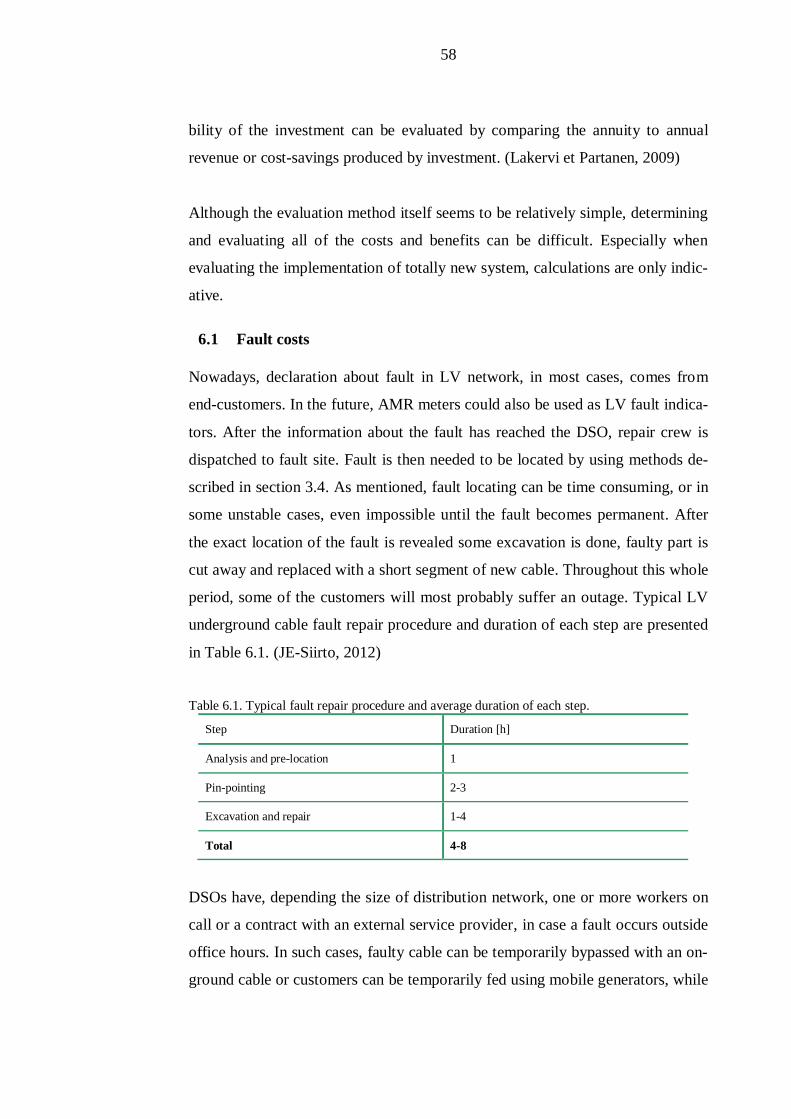
58
bility of the investment can be evaluated by comparing the annuity to annual
revenue or cost-savings produced by investment. (Lakervi et Partanen, 2009)
Although the evaluation method itself seems to be relatively simple, determining
and evaluating all of the costs and benefits can be difficult. Especially when
evaluating the implementation of totally new system, calculations are only indic-
ative.
6.1 Fault costs
Nowadays, declaration about fault in LV network, in most cases, comes from
end-customers. In the future, AMR meters could also be used as LV fault indica-
tors. After the information about the fault has reached the DSO, repair crew is
dispatched to fault site. Fault is then needed to be located by using methods de-
scribed in section 3.4. As mentioned, fault locating can be time consuming, or in
some unstable cases, even impossible until the fault becomes permanent. After
the exact location of the fault is revealed some excavation is done, faulty part is
cut away and replaced with a short segment of new cable. Throughout this whole
period, some of the customers will most probably suffer an outage. Typical LV
underground cable fault repair procedure and duration of each step are presented
in Table 6.1. (JE-Siirto, 2012)
Table 6.1. Typical fault repair procedure and average duration of each step.
Step Duration [h]
Analysis and pre-location 1
Pin-pointing 2-3
Excavation and repair 1-4
Total 4-8
DSOs have, depending the size of distribution network, one or more workers on
call or a contract with an external service provider, in case a fault occurs outside
office hours. In such cases, faulty cable can be temporarily bypassed with an on-
ground cable or customers can be temporarily fed using mobile generators, while

59
permanent repair is done later (Pavo, 2011). Thus, fault occurring during week-
end or during night, could cause two separate interruptions and increase both
labor and equipment costs.
When considering the possible benefits from OCM in LV cable networks, first
logical step is to determine the costs a fault in LV network causes to DSO. Dif-
ferent fault-cost components are:
• Outage costs
• Equipment costs
• Labor costs
• Material costs
Outage costs consist of undelivered energy and harm caused to the customers, or
HCC. Revenue loss from undelivered energy is very marginal, and therefore, it
can be ignored. Monetary value for HCC has been determined by WTA/WTP –
survey, asking customers how much damage an outage will cause to them and
how much they are willing to pay for better reliability (Silvast et al. 2005). Out-
age cost parameters, based on results from the survey, are presented in Table 6.2.
Table 6.2. Outage cost parameter for different customer types. (Honkapuro et al., 2006).Customer type Unplanned interruption Planned interruption
€ / kW € / kWh € / kW € / kWhResidential 0,36 4,29 0,19 2,21Agriculture 0,45 9,38 0,23 4,80Industry 3,52 24,45 1,38 11,47Public consumption 1,89 15,08 1,33 7,35Commercial 2,65 29,89 0,22 22,82
Monetary value of HCC is dependant from the customer types and average inter-
rupt power, outage type and outage duration. Annual HCC for network part un-
der consideration can be calculated
HCC = ( )(A + B), (6.2)
60
where P is interrupt power, f is fault rate, l is network length, A is outage cost
parameter €/kW, t is average duration of outage and B is outage cost parameter
€/kWh.
DSOs are also required to pay compensation to the customers for outages lasting
over 12 h, but average repair time for single incipient cable fault is usually below
that. Furthermore, if repair would take considerably long time, faulty cable can
be temporarily replaced with an on-ground cable, or customers can be fed using
mobile generators. Therefore, compensation payments are ruled out from consid-
eration.
Labor costs are dependent on the number of workers assigned to fault and the
total duration of repair work, including the transitions and loading/unloading
materials and equipment. Repair crew usually consists of one or two technicians
when underground LV cables are being repaired (JE-Siirto, 2012 & Pavo, 2012).
Faults occurring outside office hours will increase the labor costs. Some DSOs
have outsourced the repairs, in such case, hourly labor cost is a cost that external
service provider charges from DSO. When DSO uses its own technicians, hourly
cost of individual technician is wage plus insurances, pension contribution and
other employment costs. These costs are taken in account by multiplying the
employees hourly gross wage by a rough multiplier 1,7. Hourly wage, including
all additions, of an average network technician could be assumed to be roughly
15 €/h (CLA, 2010), therefore, estimated cost of 25 €/h per technician is used to
evaluate the labor costs.
Equipment costs consists mainly of excavating costs, operating costs of vehicles
and possible operating costs of mobile generators. Excavation costs vary consid-
erably depending on location of the fault site. Excavation in urban conditions is
more expensive and time consuming because of paved streets and traffic. There
are also numerous other underground cables and pipes running under the streets,
61
which must be taken in account. Independent contractors charge DSOs between
60 - 100 €/h for excavating (JE-Siirto, 2012 & Pavo, 2011).
Operating costs of a mobile generator consists of maintenance and fuel costs.
Fuel costs depend on the amount of energy produced, size and type of generator
and the unit price of the fuel used. Fuel consumption of modern diesel generator
is around 0,3 - 0,4 l/kWh (Diesel S&S 2011), depending on the size and load of
generator.
6.2 Benefits from OCM
Providing ‘real-time’ information about condition of the LV underground cables,
OCM can be utilized to increase the reliability of LV networks. Damaged cables
could be repaired or replaced prior to permanent fault occurs. Therefore, consid-
erable fault cost savings could be achieved with OCM -based preventive mainte-
nance.
Average duration of interruption could be decreased significantly with OCM -
based preventive maintenance. By knowing the exact spot of a defect in the ca-
ble, repair work can be prepared and planned in advance. Network technicians,
required material, and equipment can be sent to the site and damaged part can be
excavated up prior to disconnecting the cable. This will save not only interrup-
tion time, but also man-hours as time consuming fault location on site can be
avoided.
Preventive maintenance will also decrease the number of unplanned interrup-
tions. Customers can be informed in advance if interruption is needed and the
interruption can be scheduled so it causes as minimal harm to the customers as
possible. In some cases, interruption can be entirely avoided if network is inter-
connected and damaged cable can be temporarily bypassed. Also temporary on-
ground cables or mobile generators could be used to maintain service during
repairs.

62
Statistically, OCM, combined with efficient preventive maintenance system, will
decrease the number of unplanned faults as well as average duration of a fault in
LV network. This will improve the whole distribution systems reliability and
possibly in some rare cases, it could be an alternative option to more expensive
investment in MV network in order to increase the systems overall reliability.
The biggest fault cost savings will come from lower outage costs and from lower
labor costs. Unplanned interruptions could be avoided by repairing or by replac-
ing the damaged cable during planned interruption before it gets permanently
faulty. Time saved from avoided fault analysis and fault location decrease both
outage and labor costs. The effect of OCM on interruption type and duration and
on labor costs in a typical LV cable fault, based on Table 6.1, is presented in
Table 6.3.
Table 6.3. The effect of OCM on interruption type and duration and on labor costs in a typicalLV cable fault.
Cost component Without OCM [h] With OCM [h]
Unplanned interruption 4-7 -
Planned interruption - 0-2
Labor needed 5-8 2-4
There are also other minor possible savings that could be achieved by OCM.
However, estimating a monetary value to those is very difficult and in addition,
they are more speculative than those presented earlier. Therefore, they are only
described shortly and they are not included in calculations.
Once the moisture gets under the damaged cable sheath, it could propagate longi-
tudinally between the sheath and main insulation. If the insulation is intact, it
could take considerably long time before the moisture causes an electrical fault.
Over that time, the moisture propagates inside the cable and deteriorates the in-
sulation over constantly growing length. Thus, by replacing the moist section of

63
cable shortly after moisture under the sheath is detected, replacement of longer
length, or at its worst, the whole cable could be avoided.
If the damaged cable is a part of a LV network which is reached close to its max-
imum transmission capacity and thus, it is due to be renovated in the near future,
renovation could be planned and done at the same time as the damaged cable is
being replaced. Without OCM, the fault will occur without a warning and most
probably, only the faulty cable is replaced and the rest of the network is renovat-
ed later.
OCM allows also to schedule the excavation so that it causes minimal harm to
traffic. When fault occurs under street in urban areas, excavation usually requires
a permit from city officials.
Information gathered from OCM system could be also utilized in development of
installation techniques and maintenance strategies. For example, different instal-
lation techniques could be compared by the proportion of damaged cables within
a year from installation. Similar long-term test, than described in section 5.1.2,
for cables with damaged sheaths could be done in real installation conditions by
allowing a couple of damaged cables to develop an electrical fault. Results from
those tests could then be used later to determine the optimal timing when the
damaged cables should be replaced after being reported to be wet.
6.3 OCM costs
Costs from implementation of OCM system would be formed by hardware costs,
installation costs, possible data transmission costs, software update costs and
training costs of employees. System level costs, such as software updates and
training of employees are not fully dependent on the number of actual OCM sys-
tems installed. Thus, system level costs per installed OCM system will decrease
as the number of OCM systems, or on-line monitored LV networks, increase.
Evaluation of costs from implementation of totally new system is always only an
indicative estimation. However, research and practical experiences from imple-
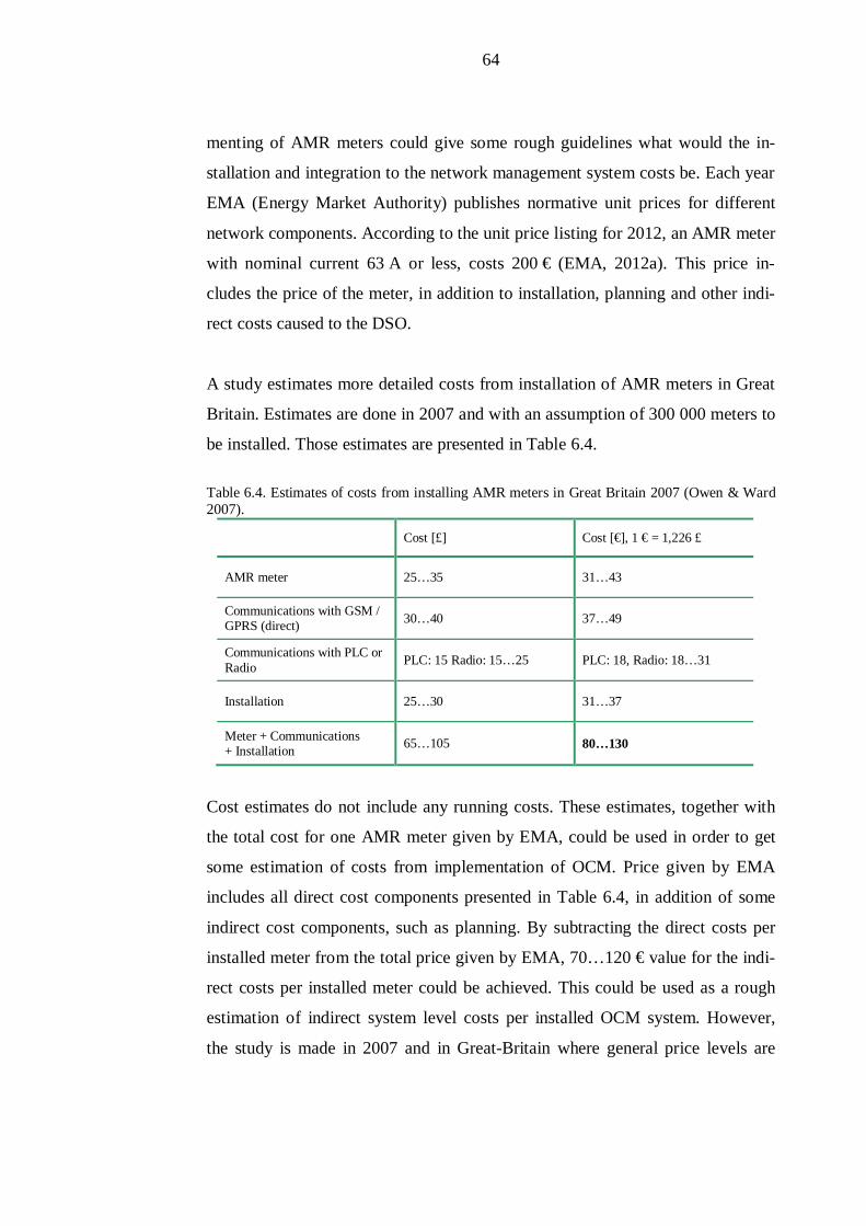
64
menting of AMR meters could give some rough guidelines what would the in-
stallation and integration to the network management system costs be. Each year
EMA (Energy Market Authority) publishes normative unit prices for different
network components. According to the unit price listing for 2012, an AMR meter
with nominal current 63 A or less, costs 200 € (EMA, 2012a). This price in-
cludes the price of the meter, in addition to installation, planning and other indi-
rect costs caused to the DSO.
A study estimates more detailed costs from installation of AMR meters in Great
Britain. Estimates are done in 2007 and with an assumption of 300 000 meters to
be installed. Those estimates are presented in Table 6.4.
Table 6.4. Estimates of costs from installing AMR meters in Great Britain 2007 (Owen & Ward2007).
Cost [£] Cost [€], 1 € = 1,226 £
AMR meter 25… 35 31… 43
Communications with GSM /GPRS (direct) 30… 40 37… 49
Communications with PLC orRadio PLC: 15 Radio: 15… 25 PLC: 18, Radio: 18… 31
Installation 25… 30 31… 37
Meter + Communications+ Installation 65… 105 80… 130
Cost estimates do not include any running costs. These estimates, together with
the total cost for one AMR meter given by EMA, could be used in order to get
some estimation of costs from implementation of OCM. Price given by EMA
includes all direct cost components presented in Table 6.4, in addition of some
indirect cost components, such as planning. By subtracting the direct costs per
installed meter from the total price given by EMA, 70… 120 € value for the indi-
rect costs per installed meter could be achieved. This could be used as a rough
estimation of indirect system level costs per installed OCM system. However,
the study is made in 2007 and in Great-Britain where general price levels are
65
different than in Finland, which could distort the comparison of these two differ-
ent prices.
Existing communications from AMR meters to secondary substation and from
secondary substation to AMR servers could be used, so communications would
not necessarily cause any extra costs. Future generation of AMR meters could be
equipped with receivers capable of receiving the high frequency measurement
signal, so only physical installations would have to be done at secondary substa-
tion. Expected lifetime of currently installed AMR meters is around 15 a, so they
need to be replaced in any case at the some point.
Hardware costs at secondary substation would be formed from high frequency
signal transmitter, OCM control system, cabling, coupling interfaces, and miscel-
laneous accessories.
Cost for high frequency signal transmitter and receivers could be estimated from
the cost of HomePlug AV –adapters. HomePlug AV –adapters utilize the PLC
technique to transfer data via internal power network of a building. Adapters use
frequency band from 2 MHz to 28 Mhz (Homeplug, 2012). Cheapest HomePlug
AV –adapters cost less than 30 € (Verkkokauppa, 2012). Thus, cost of transmit-
ter and receiver units would be minor when compared to total implementation
costs of the OCM system.
If the OCM system would be productized and those systems would be installed
to a wide range of LV networks, some company or companies would start to
manufacture and sell the OCM systems as a package. Therefore, price of such
system is not formed only from the costs of different components, but it has to
cover also all manufacturing costs and a certain net margin for the manufacturer.
Only reasonable way to get even some kind of estimation of the hardware cost of
the whole system is to look for some finished product which is even somehow
related to on-line condition monitoring of the LV networks.
66
One reference for whole hardware costs evaluation could be EDFmodGSM-230
–power quality module by MX Electrix Oy. Module is designed to be attached to
the distribution network at customers connection point or at secondary substation
and it monitors multiple power quality factors, such as phase voltages, total har-
monic distortion (THD), flickering, etc. EDFmodGSM-230 is a finished product
and it includes all necessary components to independently monitor and report the
quality of power. It can also automatically send an alarm via GSM/GPRS net-
work when preset boundaries for monitored variables are crossed. Price of an
EDFmodGSM-230 module without installation costs and VAT is 580 € (MX
Electrix, 2012).
Installation costs consists of labor costs and possible costs from a planned inter-
ruption. Installation costs are greatly dependent on that whether it is needed to
pay a visit at every customer connection point and whether it is needed to cause a
planned interruption. If customer side receiver units and possible low pass filters
are integrated to the next generation of AMR meters, it the best case scenario,
interruption could be avoided and only installation work is needed at the second-
ary substation. Installation costs could then easily be less than 100 €, if a worker
costs to the DSO 25 €/h. Otherwise, if LV network feeds, for example, 50 sepa-
rate customers and installation work is needed to be carried out at every custom-
er and planned interruptions are needed, it is clear that total implementation costs
would exceed the possible cost savings from the OCM system.
By adding up the installation costs, hardware costs and indirect costs, in the very
best case scenario, total implementation costs of OCM per LV network could be
around 1000 €. However, this would require a lot of integration to the next gen-
eration of AMR meters.
6.4 Application potential
Estimation of costs from implementation of totally new technique, as the OCM
in LV cable distribution networks would be, is really difficult. Therefore, it is
more reasonable to try to estimate how much the total implementation costs are

67
allowed to be, compared to the annual cost save potential of the system. The
maximum allowed implementation cost using different parameters can then be
compared to rough implementation cost estimates to figure out the economic
potential of the system.
Annual cost save potential from OCM is estimated based on the real fault statis-
tics from two Finnish DSOs, as well as interviews concerning the fault repair
procedures and typical durations in LV underground cable network faults. Obvi-
ously, these calculations are only indicative and they can vary considerably be-
tween different locations and companies. Therefore, sensitivity analysis is need-
ed to figure out the effect of different parameters to the results.
The following curves show the break-even point for the total implementation
costs of OCM for one LV network as a function of average interruption power
from a cable fault. Savings in outage costs, labor costs and equipment costs are
taken in account based on the information presented in sections 6.1 and 6.2.
Equations are presented in Appendix I. Following parameters are used as a
standard baseline and only the new values of parameters which are altered from
these, are presented later:
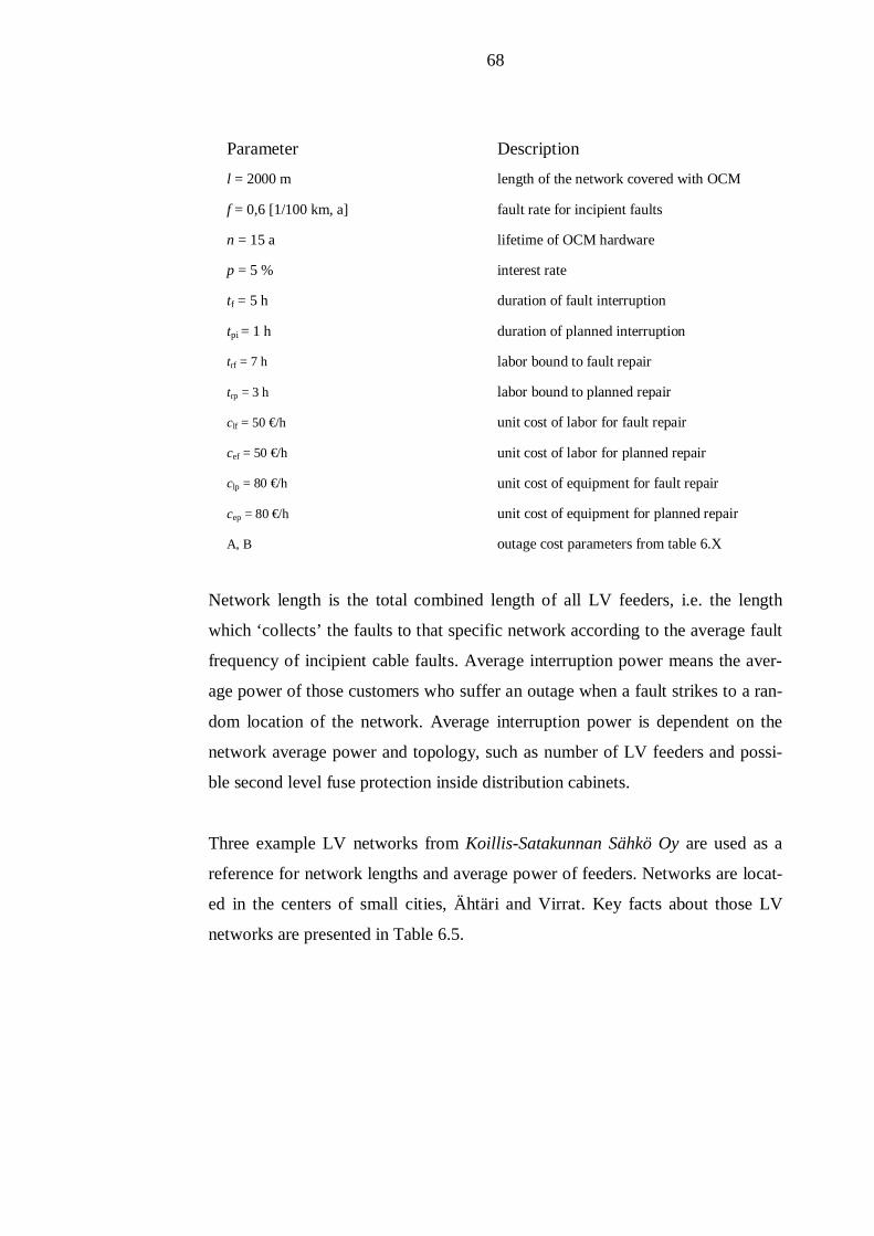
68
Parameter Description
l = 2000 m length of the network covered with OCM
f = 0,6 [1/100 km, a] fault rate for incipient faults
n = 15 a lifetime of OCM hardware
p = 5 % interest rate
tf = 5 h duration of fault interruption
tpi = 1 h duration of planned interruption
trf = 7 h labor bound to fault repair
trp = 3 h labor bound to planned repair
clf = 50 €/h unit cost of labor for fault repair
cef = 50 €/h unit cost of labor for planned repair
clp = 80 €/h unit cost of equipment for fault repair
cep = 80 €/h unit cost of equipment for planned repair
A, B outage cost parameters from table 6.X
Network length is the total combined length of all LV feeders, i.e. the length
which ‘collects’ the faults to that specific network according to the average fault
frequency of incipient cable faults. Average interruption power means the aver-
age power of those customers who suffer an outage when a fault strikes to a ran-
dom location of the network. Average interruption power is dependent on the
network average power and topology, such as number of LV feeders and possi-
ble second level fuse protection inside distribution cabinets.
Three example LV networks from Koillis-Satakunnan Sähkö Oy are used as a
reference for network lengths and average power of feeders. Networks are locat-
ed in the centers of small cities, Ähtäri and Virrat. Key facts about those LV
networks are presented in Table 6.5.
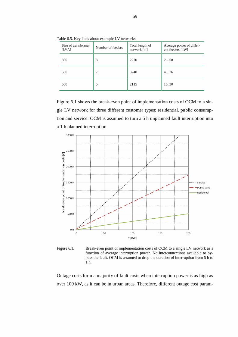
69
Table 6.5. Key facts about example LV networks.
Size of transformer[kVA] Number of feeders Total length of
network [m]Average power of differ-ent feeders [kW]
800 8 2270 2… 58
500 7 3240 4… 76
500 5 2115 16..30
Figure 6.1 shows the break-even point of implementation costs of OCM to a sin-
gle LV network for three different customer types; residential, public consump-
tion and service. OCM is assumed to turn a 5 h unplanned fault interruption into
a 1 h planned interruption.
Figure 6.1. Break-even point of implementation costs of OCM to a single LV network as afunction of average interruption power. No interconnections available to by-pass the fault. OCM is assumed to drop the duration of interruption from 5 h to1 h.
Outage costs form a majority of fault costs when interruption power is as high as
over 100 kW, as it can be in urban areas. Therefore, different outage cost param-

70
eters have major impact on the cost save potential from OCM, and thus, on the
break-even point of implementation costs.
More critical service type customers usually consume a lot more power than res-
idential type customers and they often have own secondary substations, or at
least the secondary substation is located near to them. Thus, average length of
the LV network between substation and service customer is shorter than the av-
erage length of LV network between substation and residential customer. There-
fore, the actual fault frequency which cause an interruption to service type cus-
tomers is probably lower than the average fault frequency for whole LV network.
If the duration of fault repair seems to take more than few hours, or some critical
customers, such as shops, are involved, temporary solutions like on-ground ca-
bles on mobile generators could be used to return the supply to the customers,
even though the network is not built interconnected. Therefore, Figure 6.1 pre-
sents close to a best case scenario from the OCM potential point of view, be-
cause 5 h is sufficient time to restore the supply somehow in almost any LV ca-
ble fault case.
In densely populated areas, LV networks are usually built interconnected so the
faulty cable can be bypassed by changing the switching state of the LV network.
Therefore, interruptions caused by incipient cable faults could be avoided entire-
ly by utilizing OCM in interconnected networks. At the same time, interconnec-
tions also decrease the interruption time without utilizing OCM as the supply for
majority of customers could be returned as soon as the fault is narrowed to a sin-
gle cable or to a pair of parallel connected cables. Figure 6.2 shows the break-
even point of implementation costs for three different customer types when inter-
ruption lasts 2h without OCM and when it could be avoided entirely with OCM.
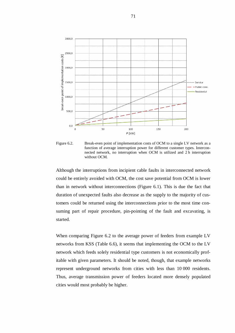
71
Figure 6.2. Break-even point of implementation costs of OCM to a single LV network as afunction of average interruption power for different customer types. Intercon-nected network, no interruption when OCM is utilized and 2 h interruptionwithout OCM.
Although the interruptions from incipient cable faults in interconnected network
could be entirely avoided with OCM, the cost save potential from OCM is lower
than in network without interconnections (Figure 6.1). This is due the fact that
duration of unexpected faults also decrease as the supply to the majority of cus-
tomers could be returned using the interconnections prior to the most time con-
suming part of repair procedure, pin-pointing of the fault and excavating, is
started.
When comparing Figure 6.2 to the average power of feeders from example LV
networks from KSS (Table 6.6), it seems that implementing the OCM to the LV
network which feeds solely residential type customers is not economically prof-
itable with given parameters. It should be noted, though, that example networks
represent underground networks from cities with less than 10 000 residents.
Thus, average transmission power of feeders located more densely populated
cities would most probably be higher.

72
Fault frequency for incipient cable faults 0,6 / 100 km, a is obtained from six
year fault statistics from two DSOs, Parikkalan Valo Oy and Rovakaira OY, to-
taling about 2300 km of LV underground cable network. Incipient faults were
filtered from the record of all cable faults by removing all abrupt faults with ob-
vious cause, for example, which were caused by an excavator. Obtained incipient
cable fault frequencies for those companies were 0,55 and 0,65 / 100 km, a.
Although it seems that the deviation in incipient cable frequency between those
companies is relatively low, the amount of data is too low for reliable statistical
analysis. Fault statistics were asked from several DSOs, but only those two com-
panies eventually provided them.
Incipient fault frequency is dependent on the average age of LV cable network,
cable types used, installation methods, average soil type and other natural fac-
tors, such as ground frost. Therefore, it can vary considerably between different
areas. Figure 6.3 shows the impact of different fault frequencies on the break-
even point of implementation costs of OCM. Network is assumed to be intercon-
nected and the average power is assumed to be divided in ratio of 70-30 between
residential type and service type customers, corresponding a typical urban LV
network.

73
Figure 6.3. Break-even point of implementation costs of OCM to a single LV network as afunction of average interruption power with different incipient fault frequen-cies [1 / 100 km, a]. Interconnected network, no interruption when OCM is uti-lized and 2 h interruption without OCM. Average power is divided between70 % residential type and 30 % service type customers.
Outage costs form a majority of fault costs in urban LV networks where average
transmission power of feeders can reach 100 kW or more. Fault frequency af-
fects directly to annual outage costs and thus, it has big impact on the cost save
potential from OCM. Differences in network lengths have exactly similar rela-
tive effect (Figure 6.4).
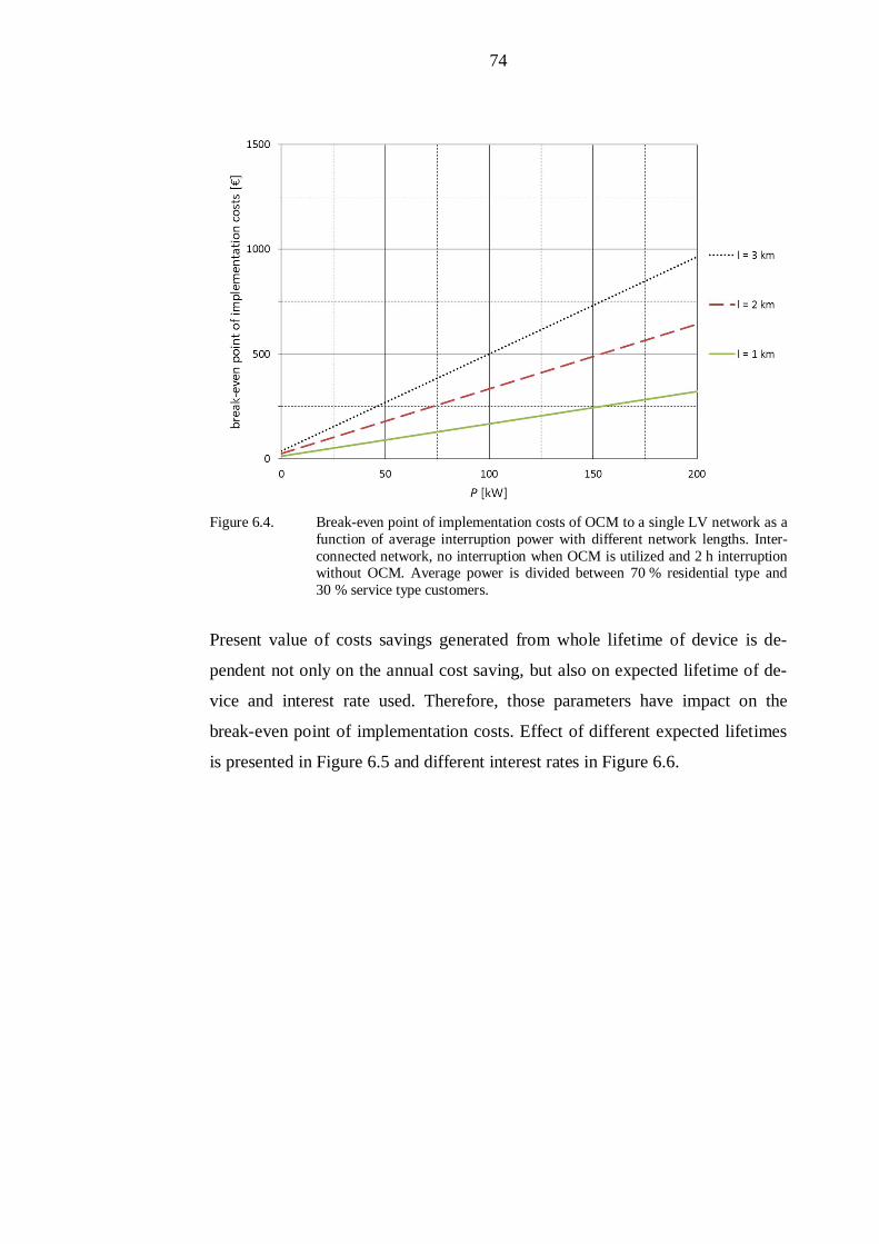
74
Figure 6.4. Break-even point of implementation costs of OCM to a single LV network as afunction of average interruption power with different network lengths. Inter-connected network, no interruption when OCM is utilized and 2 h interruptionwithout OCM. Average power is divided between 70 % residential type and30 % service type customers.
Present value of costs savings generated from whole lifetime of device is de-
pendent not only on the annual cost saving, but also on expected lifetime of de-
vice and interest rate used. Therefore, those parameters have impact on the
break-even point of implementation costs. Effect of different expected lifetimes
is presented in Figure 6.5 and different interest rates in Figure 6.6.
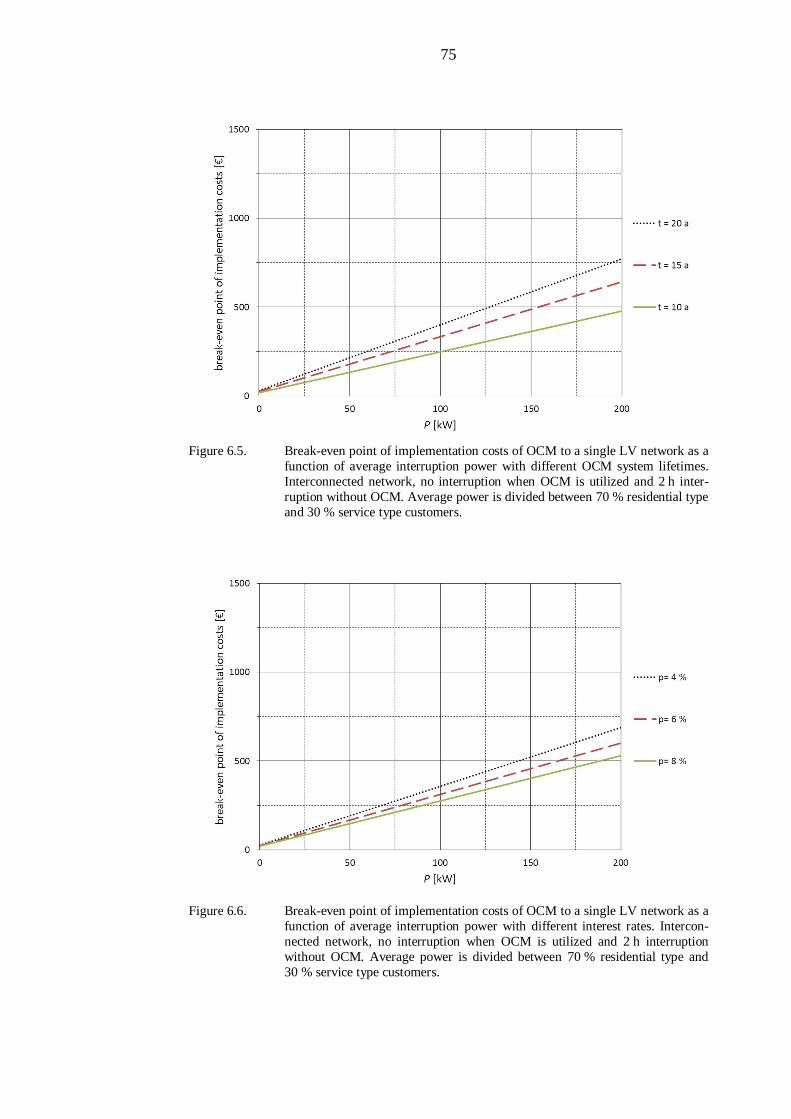
75
Figure 6.5. Break-even point of implementation costs of OCM to a single LV network as afunction of average interruption power with different OCM system lifetimes.Interconnected network, no interruption when OCM is utilized and 2 h inter-ruption without OCM. Average power is divided between 70 % residential typeand 30 % service type customers.
Figure 6.6. Break-even point of implementation costs of OCM to a single LV network as afunction of average interruption power with different interest rates. Intercon-nected network, no interruption when OCM is utilized and 2 h interruptionwithout OCM. Average power is divided between 70 % residential type and30 % service type customers.

76
As it can be seen, different values for expected lifetime or interest rate have
much less impact on the break-even implementation point than the parameters
which affects directly on the annual outage costs. Higher interest rate decreases
the present value of cost savings generated in the future and, therefore, higher
interest rate means lower break-even point of implementation costs. EMA sets
reasonable cost of capital both for community taxpayers, 4,58 % for 2012, and
for municipal electricity utilities, 4,97 % for 2012 (EMA 2012b).
Cost save potential in labor and equipment costs are so minor compared to cost
save potential in outage costs that altering those parameters would not have prac-
tically any effect on the break-even point of implementation costs.
When comparing these Figures to the implementation cost speculation in section
6.3, it could be noticed that the cases where this OCM system would be econom-
ically profitable in the current LV networks, are very limited. Especially, if the
OCM system would have to be built totally separated, it would not be profitable
investment. The more it could be integrated to other intelligent systems, for ex-
ample to the AMR or, possibly in the future, to the LVDC, the higher would be
the economic potential as the implementation costs decrease.
77
7 Conclusions
Incipient fault mechanism in modern, thermoplastic insulated LV underground
cables is relatively unstudied phenomena. Numerous different thermal, electrical,
environmental, and mechanical factors affect the durability of the cable and the
speed of fault progression. Faults in LV cables can remain unstable state for con-
siderably long periods of time. There are temporarily connected on-line TDR
devices available to detect and locate also the unstable faults.
7.1 Technical aspects of OCM system
Laboratory measurements showed that in wet conditions, it is possible to detect
and locate damage in modern thermoplastic insulated LV cables using high fre-
quency signal injection techniques. Damage could be detected prior to permanent
electrical fault develops. Theoretically, it is possible to implement an OCM sys-
tem to LV network which automatically monitors condition of cables and alarms
when cable damage is detected. Existing and expanding AMR network could be
taken advance of when implementing the OCM system.
There are many technical challenges which are needed to be solved prior to such
system could be implemented. The time it takes from the point damage first no-
ticed to the point when permanent electrical fault appears must be determined in
different installation conditions.
Frequency response fingerprint from healthy network should be able to be ob-
tained through simulations and by knowing the exact topology of the network.
Otherwise, if it is measured, OCM system could then be implemented only to
new networks where fingerprint from certainly healthy network could be meas-
ured.
Reflections from customer internal networks and effect of varying impedances
could be theoretically avoided by simple low pass series inductance filters, in-
stalled between AMR meters and customer internal networks. Customer end fil-
78
ters could be integrated to the next generation of AMR meters. Instead of using
hardware filters, it might be possible to use some intelligent algorithms to filter
out the reflections from signal. This, however, would need further research to be
done.
LVDC system would be more promising platform to implement OCM than tradi-
tional LV AC system. Reflections from customer internal networks would be
avoided because customer internal network is galvanically isolated from the dis-
tribution network. However, disturbance from the inverter units could affect the
measurement. Inverter units in LVDC system include embedded control system,
which could be utilized to control also the OCM system. Data transmission be-
tween network control room and LVDC system could be used to send declara-
tion about damaged cable.
7.2 Economic aspects of OCM system
Majority of cost save potential from implementing the OCM system to LV net-
works comes from lowered outage costs. Annual outage costs are dependent on
the number of faults per year, average duration of interruption, customer types
and average interruption power from a fault. Most promising implementation
sites would therefore be LV networks where high transmission power is divided
between limited number of feeders, total length of network would be 2 km or
more and at least one third of power is consumed by public consumption- or ser-
vice –type customers. Even then, total implementation costs of OCM for single
LV network should be less than 500 € for it to be profitable investment. It could
be said that implementation to current LV networks as a separate system would
not be profitable.
However, if the OCM system could be integrated to other intelligent systems,
such as AMR or LVDC, implementation costs would decrease and the invest-
ment to OCM system could become profitable. Reliability demands for LV net-
works could also increase in the future, if distributed generation in LV networks
79
becomes more common. This would increase the cost save potential from OCM
making it potentially profitable investment in the future.
7.3 Further research topics
The major issue to be solved before the OCM system could be implemented is
determining the correct timing of repairing the damaged cable. According to a
source, even when there is some irregular arcing present, it could take several
months until the fault becomes permanent (Clegg, 1993). Practically the only
way to determine the durability of damaged LV cables is to leave samples of
damaged cables in real LV network until permanent fault develops. However,
there are lots of different factors, such as soil properties, load profile, cable type,
etc. which most probably affect the durability of damaged cable. Therefore, or-
ganizing such real life testing would be challenging and time consuming task to
do.
Feasibility with MV cables would also be interesting subject to study. There are
many factors which makes MV network more interesting platform to implement
OCM than LV network. Potential cost savings from decreased number of faults
are much higher. MV network topology is more simple and ends of single cable
segments are usually accessible at secondary substations. Fault progression
speed is much faster once MV cable is damaged. However, structure of MV ca-
bles differ from the structure of LV cables and similar laboratory measurements
have to be carried out with MV cables than what was done with LV cables.
This thesis presented only ideas and possible difficulties regarding to implemen-
tation of the OCM system to LV networks. More specific studies and practical
tests are needed to determine how it is actually interfaced, for example, to the
AMR system, and what are the real challenges which are needed to be solved.
80
8 Summary
This thesis consists of three different parts. Fault mechanisms in modern ther-
moplastic insulated low voltage cables were researched by literature study. Two
most commonly used low voltage cables in Finnish distribution networks,
AXMK and AMCMK, were selected to be tested in laboratory. Laboratory
measurements were carried out in order to research feasibility of high frequency
signal injection techniques in on-line condition monitoring of low voltage cables.
Results show that it is possible to detect and locate damage in cable sheath when
moisture penetrates through the damaged sheath.
Economic feasibility of possible novel on-line condition monitoring methods in
LV distribution networks was studied based on the statistics and information
from Finnish distribution system operators. Economic possibilities of novel on-
line condition monitoring systems in low voltage distribution networks are very
limited, unless the implementation costs can be reduced to a level low enough.
This could be achieved, for example, by integrating the on-line condition moni-
toring system to existing systems such as the AMR, or possibly in the future, to
the LVDC.
81
References
A 1.3.2009/66 Finnish government regulation of electric
supply reporting and metering. February 5,
2009. [retrieved December 10, 2011].
From:
http://www.finlex.fi/fi/laki/alkup/2009/200
90066
Aro et al. 2003 Aro M., Elovaara J., Karttunen M., Nousi-
ainen K., Palva V. Suurjännitetekniikka.
Otatieto Oy. Helsinki. 2003. 520 p. ISBN
978-951-672-320-7
Baur 2012 BAUR Prüf- und Messtechnik GmbH.
Fault location products. [retrieved January
4, 2012]. From: http://www.baur.at/
en/products/cable-fault-location.html
Blackburn et al. 2005 Blackburn, T.R.; Phung, B.T.; Zhang Hao;
, "On-line partial discharge monitoring for
assessment of power cable insulation,"
Electrical Insulating Materials, 2005.
(ISEIM 2005). Proceedings of 2005 Inter-
national Symposium on , vol.3, no., pp.
865- 868 Vol. 3, 5-9 June 2005 doi:
10.1109/ISEIM.2005.193518
CLA 2010 Collective Labor Agreement – Energy,
ICT, Power network. 2010 [retrieved Janu-
ary 17, 2012]. From:
82
http://www.tikli.fi/Sahkoalan_tes_Energia_
ICT_Verkosto2010_2013.pdf
Clegg 1993 Clegg B. Underground CABLE FAULT
Location. McGRAW-HILL Book Compa-
ny Europe. Cambridge, UK. 1993. 349 p.
ISBN 0-07-707804-7
Densley 2001 Densley, J.; , "Ageing mechanisms and
diagnostics for power cables - an over-
view," Electrical Insulation Magazine,
IEEE , vol.17, no.1, pp.14-22, Jan.-Feb.
2001 doi: 10.1109/57.901613
Diesel S&S 2007 Diesel Service & Supply. Fuel consump-
tion chart for diesel generators, 2007 [re-
trieved January 12, 2012]. From:
http://www.dieselserviceandsupply.com/Di
esel_Fuel_Consumption.aspx
Draka 2011 Draka NK Cables Ltd. Power cables cata-
logue, 2011 [retrieved October 19, 2011].
From:
http://www.draka.fi/draka/Countries/Draka
_Finland/Languaes/suomi/navigaatio/Tuott
eet/Kiinteistoverkot/Voimakaapelit/index.h
tml
EMA 2012a Energy Market Authority. Distribution
Network Component Prices, 2012 [re-
trieved April 18, 2012]. From:
http://www.energiamarkkinavirasto.fi/files/
83
S%C3%A4hk%C3%B6njakeluverkon%20
kompo-
nenttien%20yksikk%C3%B6hinnat%20201
2.xlsx
EMA 2012b Energy Market Authority. Reasonable Cost
of Capital, 2012 [retrieved May 16, 2012].
From:
http://www.energiamarkkinavirasto.fi/data.
asp?articleid=2866&pgid=195&languageid
=246
Ensto 2011 Ensto Ltd. Underground Solutions, 2011
[retrieved November 9, 2011]. From:
http://www.ensto.com/download/19855_U
G_ENG_small.pdf
Environment 2011 Finland’s environmental administration.
Ground frost statistics, 2011 [retrieved De-
cember 2, 2011]. From:
http://www.ymparisto.fi/default.asp?node=
15166&lan=en
Gammon & Matthews 1999 Gammon, T., Matthews, J., "The historical
evolution of arcing-fault models for low-
voltage systems," Industrial & Commercial
Power Systems Technical Conference,
1999 IEEE. , vol., no., pp.6 pp., Aug 1999.
doi: 10.1109/ICPS.1999.787220
Hernandez 2012 Hernandez, C. Channel Estimation and On-
line Diagnosis of LV Distribution Cabling.
84
Master’s thesis. Lappeenranta University of
Technology. 2012.
Homeplug 2012 HomePlug Power Alliance. Frequently
asked questions, 2012. [retrieved May 14,
2012]. From: https://www.homeplug.org/
about/faqs/
Honkapuro et al. 2006 Honkapuro S., Tahvanainen K., Viljainen
S., Lassila J., Partanen J., Kivikko K.,
Mäkinen A., Järventausta P., DEA -mallilla
suoritettavan tehokkuusmittauksen kehit-
täminen. Research report. Lappeenranta.
2006.
Honkapuro et al. 2007 Honkapuro, S., Tahvanainen, K., Viljainen,
S., Partanen, J.,Mäkinen, A., Verho, P.,
Järventausta, P. Keskeytystunnuslukujen re-
ferenssiarvojen määrittäminen.EMV. 2007.
Kaipia et al. 2006 Kaipia, T., Salonen, P., Lassila, J., Par-
tanen, J. Possibilities of the Low Voltage
DC Distribution Systems. Lappeenranta
University of Technology. 2006.
Kehui 2007 Kehui. T-P22 LV Cable Fault Locator. 11
p. Handout, 2007 [retriewed January 23,
2012]. From: http://www.kehui.co.uk
/information/T-P22%20handout.pdf
85
Keränen 2009 Keränen, L. Usefulness of AMR Data In
the Network Operation. Master’s thesis.
Tampere University of Technology. 2009.
Koponen 2007 Koponen, P. AMR nykytilanne ja sen mah-
dollistamat palvelut. VTT Technical Re-
search Centre of Finland report. [retrieved
April 21, 2012] From:
http://www.vtt.fi/liitetiedostot/muut/ws1_k
oponen.pdf
Kärnä 2005 Kärnä, A. PJ -kaapeleiden soveltuvuus
1 kV käyttöjännitteelle. Master’s thesis.
Tampere University of Technology. 2005.
Lakervi & Partanen 2009 Lakervi E., Partanen J. Sähkönjakelutek-
niikka. Otatieto Oy. Helsinki. 295 p. 2009.
ISBN 978-951-672-359-7.
Livie et al. 2008 Livie, J.; Gale, P.; Anding Wang; , "The
Application of On-Line Travelling Wave
Techniques in the Location of Intermittent
Faults on low Voltage Underground Ca-
bles," Developments in Power System Pro-
tection, 2008. DPSP 2008. IET 9th Interna-
tional Conference on , vol., no., pp.714-
719, 17-20 March 2008
LVD 2006 Low-Voltage Directive LVD 2006/95/EC.
European directive, European commission,
Brussels, 2006.

86
Mäkelä 2009 Mäkelä H. Jakelumuuntajien läpi siirtyvien
ukkosylijännitteiden tarkastelu. Master’s
thesis. Tampere University of Technology.
2009.
Owen & Ward 2007 Owen G., Ward J. Smart meters in Great
Britain: the next steps? [retrieved April 21,
2012] From: http://www.esma-
home.eu/userfiles/file/downloads/Smart_M
eters_%20in_GB_july2007.pdf
Partanen et al. 2010 Partanen J., Pyrhönen J., Silventoinen P.,
Niemelä M., Lassila J., Kaipia T., Salonen
P., Peltoniemi P., Nuutinen P., Lana A.,
Haakana J., Pinomaa A., Makkonen H.,
Voutilainen V., Paajanen P., Järventausta
P., Tuusa H., Suntio T., Kannus K., Lahti
K., Nikander A., Mäkinen A., Alahuhtala
J., Suntila T., Nousiainen L., Rekola J.,
Vornanen T. Tehoelektroniikka sähkönja-
kelussa – Pienjännitteinen tasasähkönjake-
lu. Research report. Lappeenranta. 2010.
Reka 2011 Reka cables Ltd. Power Cable Installation
by Ploughing, 2011 [retrieved November
18, 2011]. From:
http://www.reka.fi/files/1454_Tyskentelyo
hje1-4kVAurauseng.pdf
Rowland & Wang 2007 Rowland, S.M.; Miao Wang; , "Fault De-
velopment in Wet, Low Voltage, Oil-
Impregnated Paper Insulated Cables," Die-
87
lectrics and Electrical Insulation, IEEE
Transactions on , vol.15, no.2, pp.484-491,
April 2008 doi: 10.1109/TDEI.2008.44834
SFS-4879 2008 0,6/1 kV voimakaapelit. PEX-eristeiset
AL- ja CU-johtimiset kaapelit. Mitoitus ja
käyttöohje. Suomen standardisoimisliitto.
52 p.
SFS-4880 2008 0,6/1 kV voimakaapelit. PVC-eristeiset ja -
vaippaiset kaapelit. Rakenne ja testaus.
Suomen standardisoimisliitto. 26 p.
SFS-6000-8-814 2007 Pienjännitesähköasennukset. Osa 8-814:
Eräitä asennuksia koskevat täydentävät
vaatimukset. Kaapelien asentaminen maa-
han tai veteen. Suomen standardisoimisliit-
to. 3 p.
Silvast et al. 2005 Silvast, A., Heine, P., Lehtonen, M., Ki-
vikko, K., Mäkinen, A.,Järventausta, P.,
Sähkönjakelun keskeytyksestä aiheutuva
haitta. Helsinki University of Technology.
2005.
Suntila 2009 Suntila T. Pienjännitekaapelien soveltuvuus
sähkönjakeluun tasajännitteellä. Master’s
thesis. Tampere University of Technology.
2009.
Valtonen 2009 Valtonen P. Interactive customer gateway
in improving the energy efficiency – con-
88
sideration of new functions and their prof-
itability Master’s thesis. Lappeenranta Uni-
versity of Technology. 2009.
Verkkokauppa 2012 Verkkokauppa.com. Price quote for ZyX-
EL PLA-4201 Mini HomePlug AV –
adapter. [retrieved May 14, 2012]. From:
http://www.verkkokauppa.com/fi/product/6
667/dgvgg/ZyXEL-PLA-4201-Mini-
500Mbps-Starter
INTERVIEWS
Ahola 2012 Professor Jero Ahola. Lappeenranta Uni-
versity of Technology. E-mail discussion
28.5.2012.
JE-Siirto 2012 Käyttöpäällikkö Sakari Kauppinen. JE-
Siirto Oy. Phone discussion. 16.1.2012
MX Electrix 2012 Tekninen johtaja Seppo Vehviläinen. MX
Electrix Oy. E-mail query. 28.4.2012
Pavo 2011 Osastopäällikkö Olli Mattila, työpäällikkö
Pekka Suomalainen. Parikkalan Valo Oy.
Parikkala. 24.11.2011

APPENDIX I Equations for break-even point graphs
Total cost of an unexpected fault, including outage costs, labor costs and equip-
ment costs:
= (A + B ) + ( + ), (I.1)
where P is interrupt power, Af is outage cost parameter €/kW for fault interrup-
tion (table 6.X), tf is duration of outage, Bf is outage cost parameter €/kWh for
fault interruption, trf is duration of repair work, clf is unit cost of labor and cef is
unit cost of equipment.
Total cost of an expected fault (with OCM implemented), including outage costs,
labor costs and equipment costs:
= A + B + ( + ), (I.2)
where Api is outage cost parameter €/kW for planned interruption, tpi is duration
of planned interruption, Bpi is outage cost parameter €/kWh for planned interrup-
tion, trp is duration of repair work, clp is unit cost of labor and cep is unit cost of
equipment.
Annual cost save potential by implementing the OCM would then be:
= ( ), (I.3)
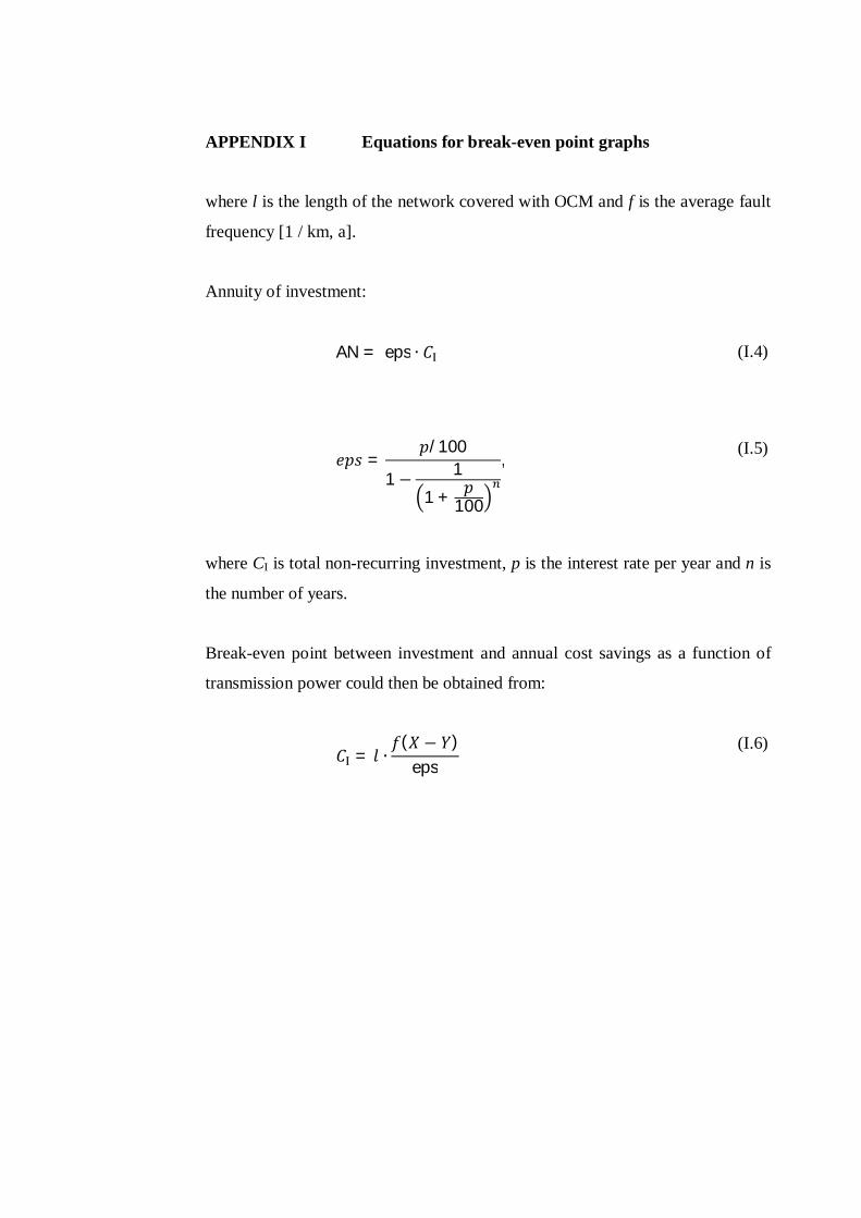
APPENDIX I Equations for break-even point graphs
where l is the length of the network covered with OCM and f is the average fault
frequency [1 / km, a].
Annuity of investment:
AN = eps (I.4)
=/100
1 11 + 100
,(I.5)
where CI is total non-recurring investment, p is the interest rate per year and n is
the number of years.
Break-even point between investment and annual cost savings as a function of
transmission power could then be obtained from:
=( )
eps(I.6)


