
Srinivas R. Chakravarthy MATH602: LECTURE 7 (WINTER 2000) 1
MATH602: APPLIED STATISTICSWinter 2000
Dr. Srinivas R. ChakravarthyDepartment of Industrial and Manufacturing
Engineering & BusinessKettering University
(Formerly GMI Engineering & Management Institute)Flint, MI 48504-4898
Phone: (810) 762-7906; FAX: (810) 762-9944
E-mail: [email protected]: http://www.kettering.edu/~schakrav

Srinivas R. Chakravarthy MATH602: LECTURE 7 (WINTER 2000) 2
RESIDUAL ANALYSIS• The methods of obtaining point and interval
estimates and tests of hypotheses, we have seen so
far tell only half the story of regression analysis.
• All of the above are done as if the model and the
underlying assumptions are reasonably correct.
• We need to do diagnostics on the model.
• The most primary concern of this is: how well the
model used resembles the data that were actually
observed?
Srinivas R. Chakravarthy MATH602: LECTURE 7 (WINTER 2000) 3
• The basic statistic we are going to see is a useful
transformation of the residuals.
• Let us first see the notion of residuals. Recall that in
the regression model (written in the matrix form): Y
= XB + E, the error component vector E was
assumed to be normal with mean 0 and variance
σ2I.
• The normality assumption is justified in many
situations since the error terms most often represent
the effects of many factors omitted explicitly from
Srinivas R. Chakravarthy MATH602: LECTURE 7 (WINTER 2000) 4
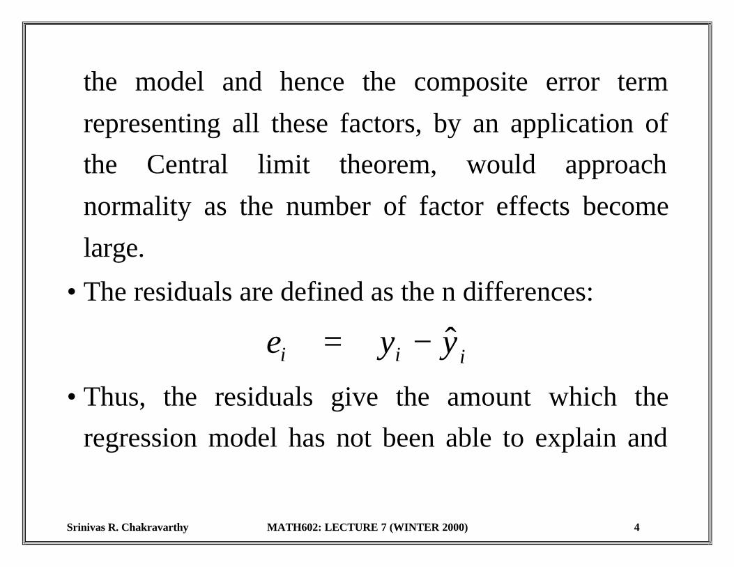
the model and hence the composite error term
representing all these factors, by an application of
the Central limit theorem, would approach
normality as the number of factor effects become
large.
• The residuals are defined as the n differences:
yye ii iˆ−=
• Thus, the residuals give the amount which the
regression model has not been able to explain and

Srinivas R. Chakravarthy MATH602: LECTURE 7 (WINTER 2000) 5
can be viewed as the observed errors if the model is
assumed to be correct.
• Now when performing the regression analysis we
have made certain assumptions about the errors;
namely, errors are uncorrelated with a mean of 0
and a constant variance and follow a normal
distribution.
• The last assumption is needed to perform F-tests
and t-tests.
Srinivas R. Chakravarthy MATH602: LECTURE 7 (WINTER 2000) 6
• Thus, if our fitted model is correct, then the
residuals should exhibit tendencies that tend to
confirm the validity of the assumptions.
• More precisely, they should not exhibit any denial
of the assumptions.
• After examining the residuals we should be able to
conclude either (1) the assumptions appear to be
violated (in a way that can be specified) or (2) the
assumptions do not appear to be violated. Note that
(2) does not imply that we are concluding that the

Srinivas R. Chakravarthy MATH602: LECTURE 7 (WINTER 2000) 7
assumptions are correct. It merely says that we have
no reason to say that they are incorrect.
• The variance, V(e) of the vector e of the residuals is
given by σ2(I - H), where H is the hat matrix.

Srinivas R. Chakravarthy MATH602: LECTURE 7 (WINTER 2000) 8
STUDY OF THE RESIDUALS
• Residuals can be used in a variety of graphical and
nongraphical summaries to identify inappropriate
assumptions.
• Generally, a number of different plots will be
required to extract the available information. The
principal ways of plotting the residuals ei are:

Srinivas R. Chakravarthy MATH602: LECTURE 7 (WINTER 2000) 9
(a) OVERALL PLOTS: When the residuals are
plotted we obtain a diagram, which if the model is
correct should, approximately, resemble observations
from a normal distribution with mean 0. Often the
histogram plot or more ideally the quantile-quantile
plot will help to determine the closeness of the
distribution of the residuals.

Srinivas R. Chakravarthy MATH602: LECTURE 7 (WINTER 2000) 10
(b) STANDARD RESIDUAL PLOTS: Standard
residual plots are those in which the residuals are
plotted against the fitted values or other functions of
x that are approximately orthogonal to the residuals.
These plots are commonly used to diagnose
nonlinearity and nonconstant error variance. The
diagrams given below in Figures 5-8 explain the
various cases that are possible.

Srinivas R. Chakravarthy MATH602: LECTURE 7 (WINTER 2000) 11
(c) PLOT AGAINST x's: The form of these plots is
the same as that against the fitted values, except that
we use the regressor variables X's instead of the fitted
values. Once again the overall impression of a
horizontal band of residuals like the one in Figure 6
is considered satisfactory.

Srinivas R. Chakravarthy MATH602: LECTURE 7 (WINTER 2000) 12
TEST FOR CONSTANCY OF
ERROR VARIANCE
• The assumption of constant variance is one of the
basic requirements in regression analysis.
• As discussed before we can detect for nonconstant
variance through a plot of the residuals against the
fitted values (see Figure 6).
• A formal statistical test can also be used.
Srinivas R. Chakravarthy MATH602: LECTURE 7 (WINTER 2000) 13
• A common reason for the violation of this
assumption is for the response variable Y to follow
a probability distribution in which the variance is
functionally related to the mean.

Srinivas R. Chakravarthy MATH602: LECTURE 7 (WINTER 2000) 14
REMEDIAL MEASURES
• If the error variance is suspected to vary in a
systematic fashion we could either (1) use the
method of weighted least square method to obtain
the estimators of the parameters of the model or (2)
use variance stabilizing transformations.
• Several commonly used variance stabilizing
transformations are given below.

Srinivas R. Chakravarthy MATH602: LECTURE 7 (WINTER 2000) 15
Variance of Yis
is proportional to
Transformation
E(Y) y
E(Y)[1 - E(Y)] ) y( sin 1−
[E(Y)]2 ln(y)
[E(Y)]3 y-1/2
[E(Y)]4 1/y

Srinivas R. Chakravarthy MATH602: LECTURE 7 (WINTER 2000) 16
ILLUSTRATIVE EXAMPLES

Srinivas R. Chakravarthy MATH602: LECTURE 7 (WINTER 2000) 17
LACK-OF-FIT TEST

Srinivas R. Chakravarthy MATH602: LECTURE 7 (WINTER 2000) 18
REMEDIAL MEASURES
If the lack of fit test concludes that the regression
model is not linear, we either
(a) search for a more appropriate model in which,we could, say, bring in a quadratic term x2 intothe model; OR
(b) use some transformation on the data so that theSLR model is more appropriate for thetransformed data

Srinivas R. Chakravarthy MATH602: LECTURE 7 (WINTER 2000) 19
ILLUSTRATIVE EXAMPLE

Srinivas R. Chakravarthy MATH602: LECTURE 7 (WINTER 2000) 20
TEST FOR INDEPENDENCE
One of the assumptions about the error terms is that
they are uncorrelated.
• To see whether this is the case, we look at the
residuals. Note that the residuals will be correlated
but serious error will be committed if they are
significantly correlated.
• We could use Durbin-Watson statistic to test for
correlation.

Srinivas R. Chakravarthy MATH602: LECTURE 7 (WINTER 2000) 21
REMEDIAL MEASURES
If the Durbin-Watson test indicates that the error
terms are correlated, we could either bring in some
additional independent variables into the model or
use transformed variables.

Srinivas R. Chakravarthy MATH602: LECTURE 7 (WINTER 2000) 22
ILLUSTRATIVE EXAMPLES

Srinivas R. Chakravarthy MATH602: LECTURE 7 (WINTER 2000) 23
TEST FOR NORMALITY

Srinivas R. Chakravarthy MATH602: LECTURE 7 (WINTER 2000) 24
TEST FOR OUTLIERS
• Since no observation can be guaranteed to be a
dependable manifestation of the problem under
study, we might see some data that may fall outside
the range of the others or that may not come from
the target distribution. These are called outliers.

Srinivas R. Chakravarthy MATH602: LECTURE 7 (WINTER 2000) 25
• The concern over outliers is old and dates back to
the first attempt to draw (statistical) conclusions
from the data.
• Outliers cannot be ignored. These may very well
contain very valuable information (imagine an
experiment involving identification of potential
sites for oil wells).
• Some times outliers might very well be data entry
errors.
Srinivas R. Chakravarthy MATH602: LECTURE 7 (WINTER 2000) 26
• Only investigators involved in the study along with
the experts of the experiment may be able to
distinguish between these two instances.
• The first thing to do is to identify the outliers.
• The commonly used method is due to Cook and is
referred to as Cook's distance measure.
• This gives an overall measure of the impact of the
i-th observation on the estimated regression
coefficients.

Srinivas R. Chakravarthy MATH602: LECTURE 7 (WINTER 2000) 27
• Naturally a large value of this measure indicates the
influence of the corresponding observation and that
could very well be an outlier.
• Note that an outliers have residuals that are large
relative to the residuals for the remainder of the
observations.

Srinivas R. Chakravarthy MATH602: LECTURE 7 (WINTER 2000) 28
REMEDIAL MEASURES
• If an outlier is identified, check (to some extent) for
the accuracy of that observation and if it is found to
be a key punch error, then it could be deleted and a
new regression model can be fitted.
• On the other hand if it is found to be a part of
genuine data, then one has to use robust procedures
to estimating the parameters.

Srinivas R. Chakravarthy MATH602: LECTURE 7 (WINTER 2000) 29
ILLUSTRATIVE EXAMPLES

Srinivas R. Chakravarthy MATH602: LECTURE 7 (WINTER 2000) 30
MULTICOLLINEARITY PROBLEM

Srinivas R. Chakravarthy MATH602: LECTURE 7 (WINTER 2000) 31
• The term multicollinearity refers to situations in which
there is almost exact linear relation among the
independent (predictor) variables.
• This is equivalent to saying that the matrix XTX is
almost singular (that is the determinant of XTX is
either 0 or very close to 0).

Srinivas R. Chakravarthy MATH602: LECTURE 7 (WINTER 2000) 32
• When this occurs the estimators tend to be inflated and
may even have incorrect sign and the predicted values
may be grossly in error.
• To detect multicollinearity, we look at variance
inflation factors, abbreviated as VIF.
• A general rule of thumb is whenever the maximum of
the VIF's does not exceed 10, assume that there is no
multicollinearity present. Otherwise, we have to
remedy the multicollinearity problem.
Srinivas R. Chakravarthy MATH602: LECTURE 7 (WINTER 2000) 33
REMEDIAL MEASURES
• See whether one or more predictor variables can be
deleted without adversely affecting the model.
• On the other hand the problem might be unique to
the particular sample obtained and observations
may not exhibit such relations.
• In this case, the variables should not be deleted and
we have to rely on ridge regression.

Srinivas R. Chakravarthy MATH602: LECTURE 7 (WINTER 2000) 34
USE OF MINITAB

Srinivas R. Chakravarthy MATH602: LECTURE 7 (WINTER 2000) 35
ILLUSTRATIVE EXAMPLES

Srinivas R. Chakravarthy MATH602: LECTURE 7 (WINTER 2000) 36
VARIABLE SELECTION AND MODEL BUILDING
• So far we have seen how to fit a regression model
given all regressor (independent) variables.
• Our focus will now be on to find a subset of
regressors, from the pool of candidate regressors,
that should include all the influential factors.
• Finding an appropriate subset of regressors for the
model is called the variable selection problem.

Srinivas R. Chakravarthy MATH602: LECTURE 7 (WINTER 2000) 37
• Building a regression model that includes only a
subset of the available regressors involves two
conflicting objectives:
(1) the model should include as many regressors as possibleso that the information content in these factors caninfluence the predicted value of y.
(2) the model should include as few regressors as possiblebecause the variance of the prediction increases as thenumber of regressors increases.

Srinivas R. Chakravarthy MATH602: LECTURE 7 (WINTER 2000) 38
• Also the more regressors there are in the model, the greaterthe costs of data collection and model maintenance.
• The process of finding a model that is a compromisebetween these two objectives is called selecting the bestregression equation.
• There is no unique definition of best and there are severalalgorithms that can be used for variable selection and belowwe shall discuss some of the commonly used algorithms.
(a) ALL POSSIBLE REGRESSIONS: This procedurerequires that the analyst fit all the regression equationsinvolving one-candidate regressor, two-candidateregressors, and so on. These equations are evaluatedaccording to some suitable criterion, such as the on that has
Srinivas R. Chakravarthy MATH602: LECTURE 7 (WINTER 2000) 39
the smallest error mean square, and the best regressionmodel is then selected. Note that this procedure requiresevaluating 2k total regression equations if there are kcandidate regressors to be considered. Clearly, the totalnumber increases exponentially as k increases.
(b) STEPWISE REGRESSION METHODS: Sinceevaluating all possible regression models can be tooinvolved computationally, especially when the number ofcandidates is large, various methods have been developedfor evaluating only a small number of subset regressionmodels by either adding or deleting regressors one at a time.These methods are generally referred to as stepwiseprocedures. They can be classified into three broad

Srinivas R. Chakravarthy MATH602: LECTURE 7 (WINTER 2000) 40
categories: (i) forward selection, (ii) backward eliminationand (iii) stepwise regression that is a combination of bothforward and backward procedures.
(i) FORWARD SELECTION: This procedure begins withthe assumption that there are no regressors in the modelother than the intercept. An effort is made to find anoptimal subset by inserting regressors into the model oneat a time. The first one selected for entry into the equationis the one that has the largest simple correlation with theresponse variable y. Suppose that this regressor is calledx1. This is also the regressor that will produce the largestvalue of the F-statistic for testing the significance of theregression [note that this F-calculated value in nothing but

Srinivas R. Chakravarthy MATH602: LECTURE 7 (WINTER 2000) 41
the square of the t-calculated value for the correspondingestimator, b1, since the square of t-random variable with rdegrees of freedom is an F-distribution with 1 (numerator)and r (denominator) degrees of freedom]. This regressor isentered if the F-statistic exceeds a pre-selected F-value.The second regressor chosen for entry is the one that hasthe largest partial F-statistic (or equivalently, that has thelargest partial correlation with y after adjusting for theeffect of the first one entered), which is given by F = SSR(x2 / x1 ) / MSE( x1, x2 )= [ SSR( x1, x2 ) - SSR( x1 ) ] /MSE( x1, x2 ).
If this value exceeds the pre-selected F-value, then x1 isentered, where we denote by x2 the regressor that produces

Srinivas R. Chakravarthy MATH602: LECTURE 7 (WINTER 2000) 42
the largest partial F-statistic. This procedure terminates eitherwhen the partial F-statistic at a particular step does not exceedthe preset F-value or when the last candidate is added to themodel.
(ii) BACKWARD ELIMINATION: While the forwardselection begins with no regressors and attempts to insertvariables until a suitable model is obtained, here theprocedure attempts to find a good model by working inthe opposite direction. That is, the model that includes allk candidate regressors is considered first. Then the partialF-statistic is computed for each regressor as if it were thelast variable to enter the model. The smallest of thesepartial F-statistics is compared with a pre-selected F-value
Srinivas R. Chakravarthy MATH602: LECTURE 7 (WINTER 2000) 43
and if the smallest F-statistic is less than the presetF-value, then that variable is removed from the model.Now a regression model with k-1 variables is fitted andthe procedure is continued until we no longer can delete avariable. Backward elimination is often a very goodvariable procedure and is particularly favored by analysts,who like to see the effect of including all the regressors,just so that nothing obvious will be missed.
(iii) STEPWISE REGRESSION: The two proceduresdiscussed above suggest the following improvement. Aregressor added at an earlier step may now be redundantbecause of the relationships between it and regressors nowin the equation. Therefore, their usefulness may be

Srinivas R. Chakravarthy MATH602: LECTURE 7 (WINTER 2000) 44
reassessed via their partial F-statistics. If a partialF-statistic for a variable is less than some other (notnecessarily the same one) preset F-value that variable isdropped from the model.
GENERAL COMMENTS
Note that none of the above procedures generally guaranteesthat the best subset regression model of any size will beobtained. Also all the stepwise procedure terminates with onefinal equation and because of this the analyst should not cometo the conclusion that the best equation is obtained. Therecould be more than one best model available for any givensituation. The order in which the regressors enter or leave

Srinivas R. Chakravarthy MATH602: LECTURE 7 (WINTER 2000) 45
does not imply the order of importance to the regressors. Infact, it is highly plausible that a regressor inserted into themodel early in the procedure may very well becomenegligible at a later stage in the procedure.
References
[1] Draper, N and Smith, H (1981). Applied regressionanalysis, 2nd Edition, John Wiley, New York.[2] Montgomery, D.C and Peck, E.A (1982). Introduction tolinear regression analysis, John Wiley, New York.[3] Neter, J and Wassermann, W (1974). Applied LinearStatistical Models, Richard D. Irwin, Inc., Illinois.

Srinivas R. Chakravarthy MATH602: LECTURE 7 (WINTER 2000) 46
[4] Cook, R.D and Weisberg, S (1982). Residuals andinfluence in regression, Chapman and Hall, New York.[5] Weisberg, S (1985). Applied linear regression, JohnWiley, NY.


