
Mathematical Theory of Boundary Layers andInviscid Limit Problem
Zhouping Xin
The Institute of Mathematical SciencesThe Chinese University of Hong Kong
International Summer School on Mathematical FluidDynamics
Levico Terme, June 27 - July 2, 2010
Zhouping Xin

CONTENT
§0 Introduction and Overview
• Boundary Conditions;• Boundary Layer Phenomena;• Survey of the Progress.
§1 Convergence Theory for no-characteristic boundary condition
§2 Convergence Theory for linearized problem in the case non-slipB.C.
§3 On Prandtl’s boundary layer equations
§4 Convergence results for Navier-Slip boundary conditions
§5 Criteria for the zero viscosity limit
§6 Asymptotic behavior of boundary layers
§7 A rigorous justification for an anisotropic viscosity case
§8 Questions and Remarks
Zhouping Xin
§0 Introduction and Overview
Problem: Determining the force of resistance experienced by asolid body moving in a fluid.
Fact: Small forces of viscous friction may perceptibly affect themotion of a fluid.
L. Prandtl: "Fluid Motion With Very Small Friction", ICM,Heidelberg, 1904.
⇒ Theory of Boundary Layers: near the physical boundary, thefluid is governed NOT by the ideal Euler system, but a"simpler" system, Prandtl system!
Zhouping Xin

References:
• H. Schlichting, Boundary Layer Theory, 7th Edition,McGraw-Hall, NY, 1987.
• O. A. Oleinik & V. N. Samoklin, Mathematical Models inBoundary Layer Theory, Chapman Hall, London, 1999.
Zhouping Xin

Let Ω be a smooth simply-connected domain in Rn with smoothboundary Γ = ∂Ω. Let the viscous fluid be governed by eitherCompressible Navier-Stokes system (CNS)
∂t ρε + div (ρuε) = 0
∂t(ρεuε) + div (ρuε ⊗ uε) +∇p(ρε) = div T ε (CNS)
whereT = µ(∇uε + (∇uε)t) + µ′(divuε)I
with
p = p(ρ), p′(ρ) > 0, ∀ρ > 0,µ = ε2, (ε > 0), µ′ = O(1)ε2,
or
Zhouping Xin

Incompressible Navier-Stokes equation (NS)∂tu
ε + (uε · ∇)uε +∇pε = ε2∆uε
∇ · uε = 0(NS)
ε: viscosity, uε: velocity, pε: pressure.
We supplement (CNS) (NS) with initial data
(ρε, uε)(x, t = 0) = (ρ0, u0)(x)(or uε(x, t = 0) = u0(x))
and various boundary conditions:(1) Nonslip:
uε|Γ = 0 (NLB)
Zhouping Xin

This is the common B.C. used frequently.
(2) Navier boundary condition (1823):uε · ~n = 0, on Γ
(D(uε)~n)τ = −αuετ
(NBC)
where τ is a tangential direction on Γ, andD(u) = (∇u+ (∇u)t).
Zhouping Xin

A very interesting special case is the vorticity free B.C.
uε · ~n = 0, (∇× uε) · τ = 0 onΓ (SNBC)
which have appeared in many problems, see Beavers-Joseph’slaw, Saffman, Serrin, Marusic-Paloka, etc.
Obviously, α→ 0, (NBC) ⇒ uε|Γ = 0 (non-slip) (NLB)
α→∞, (NBC) ⇒ uε · ~n|Γ = ∂uετ
∂~n |τ = 0 (complete slip)
Zhouping Xin

Background: Large eddy simulation (Galdi & Layton, ’00); Effective BC for a flow over a rough surface (Jager &
Mikelic, ’01); Beavers-Joseph’s law for perforatedboundaries;
Generalized Navier BC to remove the un-physicalsingularity for the motion of contact line (Qian, Wang &Sheng, ’03).
GNBCslip velocity ∼ shear stress + un-compensated Young stress
Well-posedness theory due to de Veiga (’05), Yodovitch(1963), J. L. Lions (1969), etc.
Zhouping Xin

(3) In-flow-out-flow boundary condition (Non-characteristicB.C.s):
uε = φ, φ · n 6= 0 on Γ (NCBC)
The corresponding ideal fluid is governed by either thecompressible Euler system:
∂tρ+ div (ρu) = 0∂t(ρu) + div (ρu⊗ u) +∇p = 0
(CE)
or the incompressible Euler system∂tu+ u · ∇u+∇p = 0div u = 0
(IE)
Zhouping Xin
with the same initial condition and the associated B.C.s
u · n|Γ = 0 (for NLB or NBC)
oru · n|Γ = ϕ · n 6= 0 (NCBC)
For compressible flows, more boundary conditions may beneeded depending on the sign of φ · n|Γ in the later case.
Zhouping Xin

Question: ε→ 0?
(1) Whether the viscous flow can be approximated by an idealflow? (Inviscid Limited Problem), i.e., the asymptoticrelation between viscous flow and the corresponding idealflow.
(2) What is the asymptotic behavior of the viscous solutions toIBVP uniformly up to the boundary? Are there boundarylayers?
These questions are important both theoretically and physicallydue to the appearance of the Boundary-Layer Phenomena.Indeed, due to the discrepancies of the B.C.s for the viscous andideal system, in general, there exists a thin layer near theboundary Γ = ∂Ω× (0, T ) where the velocity changesdramatically in the limit ε→ 0+.
Zhouping Xin
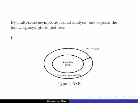
By multi-scale asymptotic formal analysis, one expects thefollowing asymptotic pictures:
I.
)()( µε OO =
Euler flow (PDE)
Prandtl’s system (PDE)
Type I. NSB
Zhouping Xin

II.
N.S. ≈ Euler
Type II. Navier type slip B.C.s
Zhouping Xin

III.
)()( 2 µε OO =
Euler System (PDE)
ODE
Type III. Non-characteristic B.C.s
Zhouping Xin

Question:
Can one justify rigorously such pictures?
=⇒ Mathematical theory of boundary layers!!
Zhouping Xin

Main Known results
Case 1: Nonslip BC
This has been the most studied case. Huge literature exists forstudies of large Reynolds number flow with no-slip B.C’s fromvarious point of views. Yet very little rigorous theory exists forthe unsteady boundary layer behavior of solutions to the N.S.for both incompressible and compressible fluids, except the caseof analytic data (Asano, Caflisch-Sarmartino) and linearizedproblems (Teman-Wang, Xin-Yanagisawa).
Zhouping Xin

(1) T. Kato (’84), R. Temam & X. M. Wang (’01) et al.:
‖uε − u‖L∞(0,T ;L2) → 0 (ZV L)
m
ε
∫ T
0‖∇uε(t)‖2L2(Γε)
dt→ 0
(Γδ = x ∈ Ω| dist(x,Γ) ≤ δ)BUT,
‖w(t, x,y
εβ)‖L2
x,y→ 0 (ε→ 0)
for any β > 0 (with Ω = x ∈ R, y > 0), so (ZVL) has no anyinformation on the behavior of boundary layers.
These criteria implies that the creation of the vorticity nearthe boundary ins the key issue to study the inviscit limitproblem.
Zhouping Xin

(2) Prandtl’s boundary layer system.
Ω = R2+ = x1, x2), x2 ≥ 0
x1
x2
~u = 0 (NS), u2 = 0 (IE)
Zhouping Xin

By applying L. Prandtl’s ansatz: (ε =√µ),
(~u, p)(x1, x2, t) = (u1, ε u2, p)(x, y, t), x = x1, y =x2
ε,
one obtains that the leading order approximations of thevelocity in the boundary layer are given by
∂t u1 + ∂x(12u2
1) + u2 ∂y u1 + ∂xp(x, t) = ν ∂2y u1
∂x u1 + ∂y u2 = 0(u1, u2)|y=0 = 0, lim
y→+∞u1(x, y, t) = U(x, t),
(PBS)
where U(x, t) and p(x, t) are determined by the correspondingEuler flow through the Bernoulli’s law
∂tU + U∂xU + ∂xp = 0. (B)
Zhouping Xin

Main Difficulty I: Well-posedness theory in Hölder Sobolev’sspaces for the IBVP of (PBS). Since (PBS) is a severelydegenerate Parabolic-elliptic system, even local in time theoryin unknown; (However, some recent progress by Gérard-Varetand Dormy) except:
Oleinik (’60) et al.: local classical solutions to (Prandtl)under certain monotonic assumption on flow;Z. P. Xin & L. Q. Zhang (’04): global classical solution to(Prandtl) under Oleinik’s monotonic assumption;
Sammartino & Caflisch (’98): well-posedness of the(Prandtl), and a rigorous justification of Prandtl’s ansatz inthe Analytic Case.
Zhouping Xin

Main Difficulty II: Even in the case that the Prandtl’s system(PBS) can be solved, the convergence of the viscous solutions asε→ 0+ still poses an extremely difficult problem due to thewidth of the boundary layer region! Even for linear problems,most of the previous works deals with L2-convergence theory forvery special flows. This forms a sharp contrast to thenon-characteristic boundary case!
Here, we will present a general result on the linearized N-Ssystem.
Zhouping Xin

Case 2: Slip Case
Convergence Yodovich (60’s), Lions (60’s): 2-d, α = +∞; Xin & Xiao (’07), da Veiga & Crispo (’09): 3-d, α = +∞; Mikelic, Iftimie, Lopes et al.: α = 1
‖uε − u‖L∞ → 0
Boundary layer: Iftimie & Sueur (’08), α = 1
‖uε − u−√εw(t, x,
y√ε)‖L∞(0,T ;L2) = O(ε)
We will present some recent results on this later.
Major problem: strong convergence for general domains!
Zhouping Xin

Case 3: In-flow-Out-flow Boundary Conditions
This is a relatively easy case at least for short time. In this case,the boundary is uniformly non-characteristic. The known resultscan be summarized as: any "weak" boundary layers are stableand the viscous solutions converge uniformly to thecorresponding Euler solutions away from the boundaries asµ→ 0+ before singularity formations.
Zhouping Xin

In particular, detailed asymptotic structure of the viscoussolutions to N.S. can be found by matched multi-scaleexpansions and justified rigorously. This theory holds for bothincompressible and compressible fluids, see X. M. Wang,Wang-Temen, Grenier, Xin, etc., Metivier-Geys, Rauch,Gilslon-Serre, Gue’s.
Some open problems in this case include: instability of strong boundary layers; interaction of singularity and boundary layers.
Zhouping Xin

Goals of this talk:(1) To study the well-posedness theory for Prandt’l boundary
layer equation.(2) Some convergence results.(3) Establish some criteria for
(ZVL)‖uε − u‖L∞(0,T ;L2) −→ 0
for all kinds of dependence of αε on ε.(4) Asymptotic behavior of boundary layers by using
multi-scale analysis.(5) Discussion of the rigorous theory on the boundary layer
behavior.
Zhouping Xin

§1 Convergence for Non-Characteristic B.C.sThis is the relatively easy case. Roughly speaking, the mostgeneral results can be stated as:
"Theorem 1.1" Assume that (NCBC) holds. Then any "weak"boundary layers are nonlinearly stable and the viscous solutionsconverge uniformly to the corresponding inviscid solutions awayfrom the boundaries as ε→ 0+ before shock singularity.
To be precise, we consider the special case:
Ω = R1+ × R1 = (x1, x2) ∈ R2, x1 ≥ 0 (1.1)
Then the NCBC becomes
u1(x1 = 0, x2, t) = f1(x2, t) > 0 (1.2)
Zhouping Xin

x2
x1
It can be shown that under suitable constraints on theamplitude of f1, (1.2) for the (CE) on the region (1.1) satisfiesthe "Uniform Lopatinski Condition", so the mixed problem for(CE), I.C. and (1.2) on Ω ((1.1)) has a unique smooth solution(ρ0, ~u0) with
(ρ0 − ρ, ~u0) ∈ C l([0, T∗) : H l+3(R1+ × R1)) (1.3)
Zhouping Xin

where l ≥ 1, and T∗ > 0 is the maximal interval of such asolution. Set
δ(T ) ≡ max[0,T ]
||u02(0, ·, t)− f2(·, t)||L∞(R1),∀T < T∗ (1.4)
In this case, "Theorem 1.1" can be stated more precisely asfollows:
Theorem 1.1 Let (ρ0, ~u0) be the solution to the IBVP for (CE)as in (1.3) with l ≥ 2. Let T ∈ (0, T∗) be fixed. Then ∃ positiveconstants δ0 and ε0 independent of ε such that if
δ(T ) ≤ δ0. (1.5)
Then ∃| solution (ρε, ~uε) to be IBVP for (CNS) such that
Zhouping Xin

(ρε − ρ, ~uε) ∈ C1([0, T ];H4(R1+ × R1)) (1.6)
and
sup0≤t≤T
x1≥h>0
||(ρε, ~uε)(x1, 0, t)− (ρ0, ~u0)(x1, ·, t)||L∞(R1) ≤ chµ ≡ chε2 (1.7)
provided that 0 < ε ≤ ε0. Furthermore, for any given n > 0,there exists a smooth bounded function
(ρ, ~u)(x, t, n, ε)
such that
sup0≤t≤T
||(ρε, ~uε)(·, t)− (ρ, ~u)(·, t)||L∞(R1+×R1) ≤ cnε
2n (1.8)
Zhouping Xin

where
(ρ, ~u)(x, t) = (ρ0, ~u0)(x, t)
+n∑
i=1
µi−1 ~Bi
(x1
µ, x2, t
)Boundary Layer Expansion,
faster dynamics
+n∑
i−1
µi~Ii(x1, x2, t)Inner Expansion,
slower dynamics
(1.9)
Remark 1.1 Due to the compatibility of the initial data andboundary date, (1.5) holds for T small. Thus, the short timeconvergence is a simple consequence of Theorem 1.1.
Zhouping Xin
Remark 1.2 (1.8)-(1.9) gives detailed asymptotic behavior ofthe solutions to the IBVP for the CNS up to any given order.Since the asymptotic solution (ρ, ~u) in (1.9) can be constructedexplicitly by the method of matched asymptotic expansions.Similar ideas have been used by Xin, Gues, Gues-Grenier, foruniform parabolic systems before.
Remark 1.3 How about the stability of strong boundarylayers? The example given by Grenier-Metwier-Rauch for anuniformly parabolic system suggests that a strong boundarylayer might be UNSTABLE!!! However, this is still OPEN forthe N-S systems. It also should be noted that this instabilitynever happens for scalar equations (Xin (1998)).
Zhouping Xin
§2 Boundary Layer Theory for Linearized System withNSB
In the case of non-slip boundary condition, NSB, the rigoroustheory of small dissipation limit problem for either CNS or INSis extremely difficult in general. Some light can be shed for thelinearized problems. For example, asymptotic analysis of Oseentype equations in a channel has been successful analyzed(Teman & Wang, IUMJ, 1996). Here we present a similartheory for the linearization of the CNS around a given profile,and justify the Prandtl’s boundary layer theory rigorously inthis case. Roughly speaking, we have
Zhouping Xin

"Theorem 2.1" Consider a linearized CNS system withnon-slip boundary conditions. Then the boundary layer isstable, and the viscous solutions converge uniformly to theinviscid solution away from the boundary.
To be precise, let’s still consider the half-space problem:Ω = R1
+ × R1. For a given smooth flow
(ρ1, u′1, u′2)(x1, x2, t) ∈ cl([0, T ],H l+2(Ω)) (2.1)
Zhouping Xin

with the property:ρ1 ≥ c0 > 0 on Ω× [0, T ]u′1(x1, x2, t) ≡ on ∂Ω× [0, T ]
(2.2)
Set
U =
P (ρ)u1
u2
(2.3)
Then the linearized N-S problem which we would like to studyis:
(LCNS) A0(U
′)∂tU
ε+
2∑j=1
Aj(U′)∂jU
2= B(ε
2, cε
2)U
εon Ω× (0, T )
(B.C.) M+Uε = 0 on ∂Ω× (0, T )
(I.C.) Uε(x, 0) = (p0, u10, u20)t ≡ U0(x) x ∈ Ω
(2.4)
Zhouping Xin
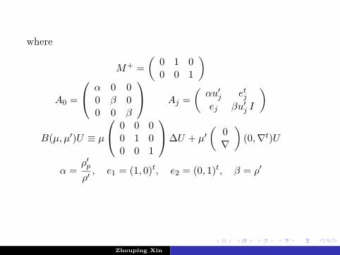
where
M+ =(
0 1 00 0 1
)A0 =
α 0 00 β 00 0 β
Aj =(αu′j etjej βu′j I
)
B(µ, µ′)U ≡ µ
0 0 00 1 00 0 1
∆U + µ′(
0∇
)(0,∇t)U
α =ρ′pρ′, e1 = (1, 0)t, e2 = (0, 1)t, β = ρ′
Zhouping Xin

The corresponding linearized inviscid problem isA0(U ′)∂tU
0 +2∑
j=1
Aj(U ′)∂jU0 = 0 Ω× (0, T ) (LCE)
M0 U0 = 0U0(x, t = 0) = U0(x)
(2.5)
where
M0 = (0, 1, 0). (2.6)
Zhouping Xin

Assume that the I.C. is compatible with the boundaryconditions in (2.4)-(2.5) up to higher order. Then thewell-posedness of both problems (2.4) and (2.5) in the Sobolevspace
C l([0, T ],Hm(Ω))
can be established quite easily. The goal is to give a Pointwiseestimate between U ε and U0. In this case, our "Theorem 2.1"can be stated more precisely as
Theorem 2.1 Assume U0 is compatible with the B.C.,M+ U = 0. Let U0 ∈ cl([0, T ];Hm(Ω)) be the unique solutionto the IBVP (2.5) for any 0 < T <∞. Then the unique smoothsolution U ε to the IBVP (2.4) admits the following estimates:
Zhouping Xin

sup0≤t≤T
x1≥hε1−δ
x2∈R1
|ρ2 − ρ0|(x1, x2, t) +2∑
j=1
|u2j − u0
j |(x1, x2, t)
≤ cδhε (2.7)
where h > 0 is any finite number, 0 < δ < 1, 0 < ε < 1, and cεhis a positive constant independent of ε. Furthermore, thefollowing asymptotic ansatz:
U2(x, t) ∼ U0 +∑i≥1
εi Ii(x1, x2, t) +∑j≥0
εj Bj(x1
ε, x2, t) (AA)
can be constructed and justified up to any order!
Remark 2.1 Similar conclusions hold for linearizedincompressible N-S system.
Zhouping Xin

Remark 2.2 The main tools are:Matched Asymptotic Analysis + Weighted Energy EstimatesThe key is to estimate a linearized Prandtl’s boundary layersystem. We can show that the linearized Prandtl’s system iswell-posed in a weighted Sobolev space. However, it should benoted that our estimate here is not enough to handle thenonlinear problem!
Remark 2.3 The nonlinear problem is still completely open!
Remark 2.4 The asymptotic ansatz (AA) can be constructedby multi-scale matched asymptotic analysis. The inner functions(boundary layer) and the outer functions can be constructedsimultaneously by solving IBVP’s for linearized Prandtl’ssystems and CE system.
Zhouping Xin

§3 On Prandtl’s boundary layer equationsFor NSB, it is expected that the leading order approximation ofthe flow velocity in the boundary layer is governed by thePrandtl’s system. Thus the solvability of this system in thestandard Hölder or Sobolev’s spaces is of fundamentalimportance. Along this line, the major previous rigorous resultsare due to Oleinik, who gives some “local” well-posedness theoryin Holder space for a class of data (monotonic data).
Zhouping Xin

∂tu+ u∂xu+ v∂yu+ ∂xp = ν∂2
y u
∂x u+ ∂yv = 0(3.1)
R = (x, y, t), 0 ≤ x ≤ L, 0 ≤ y < +∞, 0 ≤ t < T (3.2)
The initial condition (I.C.)
u|t=0 = u0(x, y) (3.3)
Zhouping Xin

To be precise, consider a plane unsteady flow of viscousincompressible fluid in the presence of an arbitrary injection andremoval of the fluid across the boundaries.
εYy =
Zhouping Xin

The boundary conditions:u|x=0 = u1(y, t), v|y=0 = v0(x, t)u|y=0 = 0, limy→+∞ u(x, y, t) = U(x, t)
(3.4)
where the pressure p = p(x, t) is given by the Bernoulli’s law:
∂tU + U∂xU + ∂xp = 0 (3.5)
with U = U(x, t) determined by the corresponding Euler flow.
Zhouping Xin
The class of data studied by Oleinik is described as
(H1) : U > 0, u0 > 0, u1 > 0, and v0 ≤ 0; and the data arecompatible.
(H2) (Monotonicity): ∂yu0 > 0, ∂y u1 > 0
Under the assumptions (H1) and (H2), O. A. Oleinik and hercollaborators have obtained a series of results, which can besummarized as:
Zhouping Xin

Oleinik’s Theorem:
Under the assumptions (H1) and (H2) on the data, ∃1 classicalsolution (u, v) to the IBVP (3.1)-(3.4) in the domain R providedthat TL is suitably small. The derivatives ∂t u, ∂x u, ∂y u, ∂2
y u,and ∂y v are all continuous in R; moreover, the ration ∂2
y u/∂y uand (∂3
y u ∂y u− ∂2y u)/(∂y u
3) are bounded in R.
One of the open problems listed at the end of the book writtenby Oleinik and Sarmokin is:
What are the conditions ensuring the existence and uniquenessof a solution of the nonstationary Prandtl’s system in the regionR with arbitrary T and L?
Zhouping Xin

The following are some recent results to answer this question:
Theorem 3.1 (Xin-Zhang, 2004)Assume that
1. (H1) and (H2) hold;2. ∂xp(x, t) ≤ 0, (Pressure favorable)
Then the IBVP, (3.1)-(3.4), has a global bounded weak solutionwhich is Lipsehitz continuous in both space and time.
In fact, such a solution is unique. Indeed,
Theorem 3.2 (Xin-Zhang-Zhao)Under the same assumptions as in the Theorem 2.1, the weaksolution depends on the data continuously. In particular, such aweak solution is unique!More recently, we have shown such a weak solution is in fact aclassical solution.
Zhouping Xin

Theorem 3.3 (Xin-Zhang-Zhao)Under the same assumptions as in Theorem 3.1, the uniqueweak solution to the IBVP, (3.1)-(3.4), is smooth in the interiorof R. Furthermore, if the data are smooth then the weaksolution is a classical solution!
Remark 3.1 The boundary condition, ∂xp ≤ 0, is calledpressure favorable, is the stability condition for stationarylaminar boundary layers.
Remark 3.2 The monotonicity assumption (H2) is crucial inthe Theorem 3.3. Indeed, in the case ∂xp ≡ 0, Weinan E andBjorn Engquist have shown that a smooth solution to thePrandtl’s system may blow-up in finite time without (H2).Indeed, in the case that (H2) does not hold, even the localexistence of solution has not been established.
Zhouping Xin

Sketch of The AnalysisUsing the generalized Crocco transformation
τ = t, ξ = x, η =u(x, y, t)U(x, t)
, w =∂y u(x, y, t)U(x, t)
, (3.6)
one can transform the original IBVP (3.1)-(3.4), into∂τw + ηU∂ξ w +A∂η w +Bw = νw2 ∂2
η w, on Ωw|τ=0 = ∂y u0
U ≡ w0, w|η=1 = 0w|ξ=0 ≡ w1 ≡ ∂y u1(y,t)
U(0,t) , (νw∂η w − u0w)|η=1 = ∂x pU
(3.7)
where Ω = (ξ, η, τ); 0 < τ <∞, 0 < η < L, 0 < η < 1
A = (1− η2)∂x U + (1− η)∂t U
U, B = η∂x U +
Ut
U(3.8)
Zhouping Xin

Set
ΩT = (ξ, η, τ) : 0 < τ < T, 0 < ξ < L, 0 < η < 1
Definition (Weak solution):A function w ∈ BV (ΩT ) ∩ L∞(ΩT ) is said to be a weak solutionto the problem (3.7) if(i) ∃C = C(T ) > 0 such that
C−1(1− η) < w(ξ, η, τ) < C(1− η), on ΩT (3.9)
(1− η)12 ∂η w ∈ L2(ΩT ), (3.10)
(ii) ∂2η w is a locally bounded measure in ΩT , and∫ ∫
ΩT
(1− η)2 d|wηη| <∞ (3.11)
Zhouping Xin

(iii) The boundary conditions in (3.7) are satisfied in the senseof trace;
(iv) For any ϕ ∈ C1(ΩT ) with ϕ|τ=0 = ϕ|ξ=0 = ϕ|ξ=L = 0, thefollowing identify holds:
−∫w−1 ϕ(1− η)2 dξ dη|τ=τ +
∫∫ΩT
w−1(1− η)2 ∂τ ϕdξ dη dτ
+∫∫
ΩT
((1− η)2 ϕ)η wη dξ dη dτ +∫∫
ΩT
(ηUϕ)ξ (1− η)2 w−1 dξ dη dτ
+∫∫
ΩT
((1− η)2Aϕ)η w−1 dξ dη dτ +
∫∫ΩT
(1− η)2 ϕBw−1 dξ dη dτ
+∫ τ
0
∫ L
0
v0(ξ, τ)ϕ(ξ, η = 0, τ)dξ dτ = 0
Zhouping Xin

Then, the main conclusions, Theorems 3.1-3.3, follow from thefollowing Proposition:
Proposition 3.4 Assume that the data satisfy (H1), (H2), andpressure being favorable. Then
1. There exists a weak solution w ∈ BV (ΩT ) ∩ L∞(ΩT ) to(3.7) in the sense of the definition. Furthermore, ∀α > 0,
(1− η)α−1
2 ∂η w ∈ L2(ΩT ),∫ ∫ΩT
(1− η)α d|wηη| < +∞.
Zhouping Xin
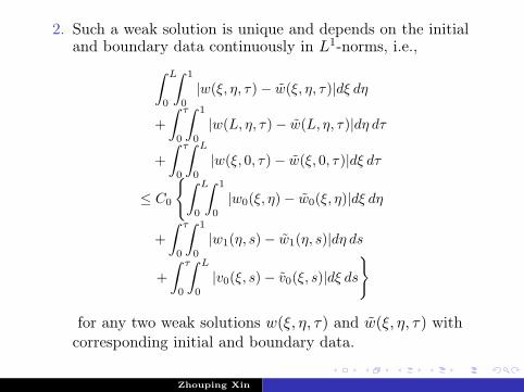
2. Such a weak solution is unique and depends on the initialand boundary data continuously in L1-norms, i.e.,∫ L
0
∫ 1
0
|w(ξ, η, τ)− w(ξ, η, τ)|dξ dη
+∫ τ
0
∫ 1
0
|w(L, η, τ)− w(L, η, τ)|dη dτ
+∫ τ
0
∫ L
0
|w(ξ, 0, τ)− w(ξ, 0, τ)|dξ dτ
≤ C0
∫ L
0
∫ 1
0
|w0(ξ, η)− w0(ξ, η)|dξ dη
+∫ τ
0
∫ 1
0
|w1(η, s)− w1(η, s)|dη ds
+∫ τ
0
∫ L
0
|v0(ξ, s)− v0(ξ, s)|dξ ds
for any two weak solutions w(ξ, η, τ) and w(ξ, η, τ) withcorresponding initial and boundary data.
Zhouping Xin

3. Such a weak solution w(ξ, η, τ) is smooth in the interior ofΩT , and if the data are smooth, then it is a classicalsmooth solution!
Remark 3.3 The existence of BV (Ωτ ) ∩ L∞(Ωτ ) solution canbe proved by at least two ways, splitting method of Xin-Zhang(2004), or by TV uniform estimate as follows:
We approximate (3.7) by (taking ν = 1)∂τ u− (u+ ε)2 ∂2
η u+ (ηu+ ε)∂ξ u+A∂η u+Bu = 0u|τ=0 = uε
0, u|ξ=0 = uε1, uε|η=1 = 0,
(u+ ε)∂η u|η=0 = (vε0(u+ ε) + ∂ε p
U )|η=0
(3.12)
with uε0, u
ε1, and vε
0 being suitable regularization of u0, u1, andv0 respectively.
Zhouping Xin

Then one can show that
c+1 (1− η) ≤ uε(ξ, η, τ) ≤ c1(1− η), ∀(ξ, η, τ) ∈ QT . (3.13)
∫QT
|∇uε(ξ, η, τ)dξ dη dτ ≤ c2(QT ) (3.14)
with c1 and c2 independent of ε. Here (3.13) follows fromcomparison arguments while (3.14) involves weighted avergingestimate on the gradient! Then the existence follows fromtaking the limit ε→ 0+. However, the arguments for theuniqueness and continuous dependence are a bit morecomplicated. The main strategy is show a L1-contraction forweak solutions to (3.7) motivated by the pioneering work ofKrushkov by using Krushkov entropy and BV calculus!
Zhouping Xin
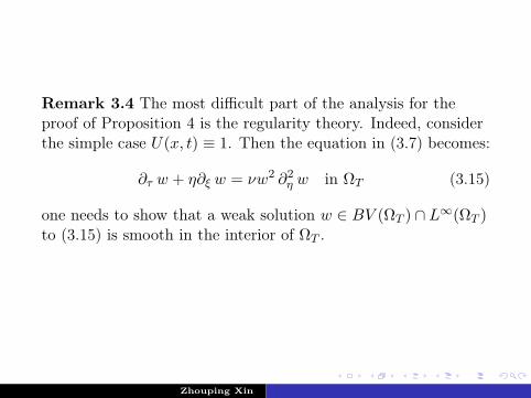
Remark 3.4 The most difficult part of the analysis for theproof of Proposition 4 is the regularity theory. Indeed, considerthe simple case U(x, t) ≡ 1. Then the equation in (3.7) becomes:
∂τ w + η∂ξ w = νw2 ∂2η w in ΩT (3.15)
one needs to show that a weak solution w ∈ BV (ΩT ) ∩ L∞(ΩT )to (3.15) is smooth in the interior of ΩT .
Zhouping Xin

Note thatL0 = ∂2
η − ∂τ + η∂ξ
is a hypoelliptic operator and δλ-homogeneous of degree 2 withsome dialation group δλλ>0
δλ = diag (λ3, λ, λ2)
(∵ rank Lie (∂η, ∂τ + η∂x) = 3)Thus, the regularity theory can be reduced to study theCα-regularity of weak solution to
∂τ w + η∂ξ w = A∂2η w, A ∈ L∞ (3.16)
Zhouping Xin

(3.16) is a typical ultraparabolic equation while has been studiedextensively, see L. P. Kupcov (1977), Lanconelli-Polidoro (1994),Polidoro (1998), Mantredini-Polidoro (1998), etc..
Some of the main difficulties:1. Caccioppoli estimates ; H1-estimate;2. ⇒ one cannot use Sobolev inequalities to do the
Nash-Moser iteration;3. Even the one-side Nash-Moser iteration can be obtained, it
seems difficult to apply John-Nirenbergy inequality?
Zhouping Xin

Sketch of the regularity analysis (Krushkov’s entropyestimates)Consider the Cα-regularity of the solution of
∂tu+ y∂xu− (Auy)y = 0, y > 0, (3.17)
at the point (x, y, t) = (0, 1, 0). Let r > 0, and
Br = (x, y, t)||x−t| ≤ r3, |y−1| ≤ r, |t| ≤ r2, B+r = Br∩t ≤ 0
Assume that A ∈ L∞(B1) so that for a positive constant λ,
λ−1 < A < λ in B1.
Define for 0 < α, β, r < 1,
Ktr = (x, y)||y − 1| ≤ r, |x− t| ≤ r3
Ktβr = (x, y)||y − 1| ≤ βr, |x− t| ≤ (βr)3
Zhouping Xin
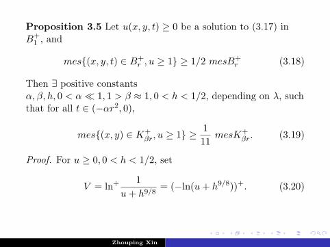
Proposition 3.5 Let u(x, y, t) ≥ 0 be a solution to (3.17) inB+
1 , and
mes(x, y, t) ∈ B+r , u ≥ 1 ≥ 1/2 mesB+
r (3.18)
Then ∃ positive constantsα, β, h, 0 < α 1, 1 > β ≈ 1, 0 < h < 1/2, depending on λ, suchthat for all t ∈ (−αr2, 0),
mes(x, y) ∈ K+βr, u ≥ 1 ≥ 1
11mesK+
βr. (3.19)
Proof. For u ≥ 0, 0 < h < 1/2, set
V = ln+ 1u+ h9/8
= (−ln(u+ h9/8))+. (3.20)
Zhouping Xin
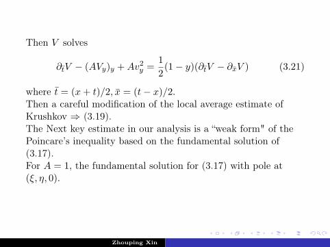
Then V solves
∂tV − (AVy)y +Av2y =
12(1− y)(∂tV − ∂xV ) (3.21)
where t = (x+ t)/2, x = (t− x)/2.Then a careful modification of the local average estimate ofKrushkov ⇒ (3.19).The Next key estimate in our analysis is a “weak form" of thePoincare’s inequality based on the fundamental solution of(3.17).For A = 1, the fundamental solution for (3.17) with pole at(ξ, η, 0).
Zhouping Xin

Γ0(z, (ξ, η, 0))
=
√3
2πt2exp
− (y−η)2
4t − 3t3
(x− ξ − t2(y + η)2)
, t > 0
0, t ≤ 0.(3.22)
Here z = (x, y, t). Then Γ0(z, ζ) is the fundamental solution withpole at ζ = (ξ, η, τ) given as in (3.22) with t replaced by t− τ.Define a ball Br centered at (0, 1, 0) as
Br = (x, y, t)||x−ty| < r3, |y−1| < r, |t| ≤ r2, B+r = Br∩t ≤ 0,
Ktr = (x, y)||x− ty| ≤ r3, |y − 1| ≤ r.
Zhouping Xin

Then Br, Ktr are equivalent to Br,K
tr respectively.
Then Proposition 3.5 impliesCorollary 3.1: Under the same assumption as in Proposition3.5, it holds that ∀t ∈ (−αr2, 0),
mes(x, y) ∈ Ktβr, u ≥ h ≥ 1
12mesKt
βr (3.23)
Zhouping Xin

Proposition 3.6 Let w be a nonnegative weak subsolution to(3.17) in B1. Then ∃ constant C = C(λ) such that∫
B+θr
[(w(z)− I1)+]2 ≤ Cr2
(1− θ)2
∫B+
r
|∂yw|2dy (3.24)
where I1 = maxz∈B+θrI1(z) with
I1(z) =∫
B+r
∂ηψ(ζ)∂ηΓ0(z, ζ)w(ζ)dζ
+∫
B+r
(∂τψ(ζ) + η∂ηψ(ζ))Γ0(z, ζ)w(ζ)dζ(3.25)
ψ(z) = ψ(x, y, t)
= χ([110
((y − 1)2
4t2 + 3(x− y + 1
2t)2 − 3tr4)]1/6)χ(
|t|1/2
θ3)
(3.26)
Zhouping Xin

χ ∈ C∞([0,∞)) such thatχ(s) = 1, if s < 2θr,χ(s) = 0, if s > r,
0 ≤ χ′(s) ≤ 2(1−2θ)r , if 2θr < s < r.
Remark 1) If u is a solution to (3.17), then w = (ln hu+h9/8 )+ is
a subsolution, so one can apply Proposition 3.6 to w.2) (3.24) yields a Poincare type inequality for a subsolution to(3.17).
Zhouping Xin

Lemma 3.7 Under the assumption of Proposition 3.5, ∃ anabsolute constant λ0, 0 < λ0 < 1 such that
|I0| ≤ λ0ln(1h1/8
) (3.27)
This follows from the structure of Γ0 and ψ and the followingfacts:
1 =∫
B+βr
∂ηψ∂ηΓ0(z, ·)dζ +∫
B+βr
(∂τψ+ η∂ξψ)Γ0(z, ·)dζ,∀z ∈ B+θr
(3.28)
mes(B+βr\B
+θr)∩z|u ≥ h ≥ 1
15mesB+
βr, for suitably small θ(3.29)
Zhouping Xin

Based on Propositions 3.5, 3.6, and Lemma 3.7, it can be shownthatProposition 3.8 Suppose that u ≥ 0 be a weak solution to(3.17) in B+
1 and the condition (3.18) is satisfied. Then thereexist positive constants θ and h0, 0 < h0, θ < 1, depending onlyon λ, such that
u(x, y, t) ≥ h0 in B+θr.
Zhouping Xin
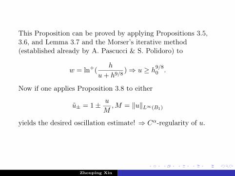
This Proposition can be proved by applying Propositions 3.5,3.6, and Lemma 3.7 and the Morser’s iterative method(established already by A. Pascucci & S. Polidoro) to
w = ln+(h
u+ h9/8) ⇒ u ≥ h
9/80 .
Now if one applies Proposition 3.8 to either
u± = 1± u
M,M = ‖u‖L∞(B1)
yields the desired oscillation estimate! ⇒ Cα-regularity of u.
Zhouping Xin

§4 Convergence results for Navier-Slipboundary conditionsThe 3-dimensional incompressible N-S system can be written as
∂t u− µ∆u+ w × u+∇p = 0 in Ω∇ · u = 0, w = ∇× u
(4.1)
with initial data
u|t=0 = u0(x) (I.C.) (4.2)
and a slip boundary condition:
u · n = 0, w × n = 0 on ∂Ω (4.3)
Zhouping Xin

It can be shown that
⇐⇒ u · n = 0, ∂n uτ = 0 ⇐⇒ (4.4)
⇐⇒ u · n = 0, (D(u)n)τ = −kτ uτ (4.5)
where kτ is the corresponding principal curvature of theboundary ∂Ω.
We will assume that Ω ⊂ R3 is a simply connected, boundedsmooth domain.
Zhouping Xin

Set
D(Ω) = C∞(Ω)Dτ (Ω) = u ∈ D(Ω); ∇ · u = 0, u · n = 0Dn(Ω) = u ∈ D(Ω); ∇ · u = 0, u× n = 0D0(Ω) = u ∈ C∞0 (Ω); ∇ · u = 0Hs
τ (Ω) = u ∈ Hs(Ω); ∇ · u = 0, u · n = 0, s ≥ 0Hs
n(Ω) = u ∈ Hs(Ω) ∩H; ∇ · u = 0, u× n = 0, s ≥ 1W = u ∈ H2
τ (Ω); (∇×)u ∈ H1n(Ω).
Zhouping Xin

Then our first convergence result is as follows:
Theorem 4.1 (Xiao-Xin, 2007) Assume that1. Let Ω = [0, 1]2per × (0, 1).2. u0 ∈W ∩H3(Ω)⇒ ∃T0 independent of µ such that(i) The problem (4.1)-(4.3) has a unique strong solution u with
the properties (ε =√µ)
uε ∈ L2(0, T0;H4(Ω))∩C([0, T0];H3(Ω)), uε ∈ L2(0, T0 : W )
Zhouping Xin

(ii) As ε =√µ→ 0+,
uε −→ u0 in L∞(0, T0; H3(Ω))uε −→ u0 in C([0, T0]; H
52 (Ω))
and u0 ∈ C([0, T0]; H52 (Ω)) is a unique solution to
∂t u+ w × u+∇p = 0∇ · u = 0, w = ∇× u
in Ω
with I.C. u|t=0 = u0
and B.C. u · n = 0 on ∂Ω.(iii) The following convergence rate holds:
sup0≤t≤T0
||uε − u0||22 ≤ Cε on [0, T0]
Zhouping Xin

However, for general simply-connected bounded domains, wecan only obtain the following result:
Theorem 4.2 Assume that1. u0 ∈W ∩H3(Ω), and ∇× u0|∂Ω = 0.2. u(x, t) is a smooth solution to the Euler system on [0, T ],T > 0.
Then ∃ ε0 > 0, such that for all ε ≤ ε0, the problem (4.1)-(4.3)has a unique solution uε(x, t), t ∈ [0, T ] satisfying
sup0≤t≤T
||uε(·, t)− u(·, t)||21 + ε
∫ T
0||uε − u||22dt ≤ cε2
Zhouping Xin

Remark 4.1 In fact, it is not too difficult to show that if theideal Euler system has a smooth solutionu0 ∈ c1([0, T ],H5(Ω)) ∩ L2([0, T ],H6(Ω)) satisfying theboundary condition u0 · n|∂Ω = 0 for some T > 0, then theviscous problem, (4.1)-(4.3), has a unique solutionuε ∈ C([0, T ],H1(Ω)) ∩ L2([0, T ],H2(Ω)) for each fixed ε > 0such that
||uε − u0||0 ≤ cε14 (4.6)
and
uε · n = 0, (D(uε) · n)τ = αuετ (4.7)
Zhouping Xin

for any fixed constant α. However, in general, the convergencein (3.6) can not hold true for stronger norms, there will beboundary layers.
Remark 4.2 In the general Navier-slip boundary condition, αmay depend on Reynolds number, α = α(Re). See Section 6.
Example α = (Re)γ = 0(1)µ−γ . Then similar convergencetheory can be obtained for γ < 1
2 with varies order of boundarylayer conditions! (Wang-Wang-Xin)
Zhouping Xin
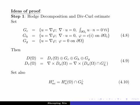
Ideas of proof:Step 1: Hodge Decomposition and Div-Curl estimateSet
Gc = u = ∇ϕ; ∇ · u = 0,∫∂Ωi
u · n = 0∀iGh = u = ∇ϕ; ∇ · u = 0, ϕ = c(i) on ∂ΩiGg = u = ∇ϕ; ϕ = 0 on ∂Ω
(4.8)
Then
D(Ω) = Dτ (Ω)⊕Gc ⊕Gh ⊕Gg
Dτ (Ω) = ∇×Dn(Ω) = ∇× (Dn(Ω) ∩G⊥h )(4.9)
Set also
Hsnc = Hs
n(Ω) ∩G⊥h (4.10)
Zhouping Xin

Lemma 1 Let u ∈ D(Ω), ∀ ∈ N . Then
||u||s ≤ c(||∇ × u||s−1 + ||∇ · u||s−1 + |uτ |s− 12
+ ||u||s−1) (4.11)
=⇒ ||u||s ≤ c(||∇ × u||s−1 + ||u||s−1) (4.12)if u ∈ Dτ (Ω) or u ∈ Dn(Ω), s ∈ N.
Lemma 2 Let u ∈ H1nc(Ω). Then
||u|| ≤ c(||∇ × u||)=⇒ ||u||s ≤ c||∇ × u||s−1 (4.13)
if u ∈ Hsnc(Ω) and s ∈ N. (4.14)
Zhouping Xin

As a consequence
(∇× u, h) = (u,∇× h) = 0 ∀u ∈W, h ∈ Gh
Thus ∇×∇× : W 7−→ H1nc(Ω) −→ H0
τ (Ω).
Proposition 4.3 The Stokes operator −∆ : W 7−→ H0τ (Ω) is
bijective and bounded, and its inverse (−∆)−1 is symmetricpositive and compact is H0
τ (Ω) with
(−∆)−1 (Hsτ (Ω)) = Hs+2
τ (Ω) for s ≥ 0
In fact, −∆ is self-adjoint on H0τ (Ω) with D(−∆) = W .
Zhouping Xin

Step 2: Compatibility of the Nonlinearity with the B.C.Set
w = ∇× u,B(u) = w × u+∇p.
Proposition 4.4 B(u) ∈ D(Ω) ∩W if u ∈ D(Ω) ∩W .
Step 3: Galenkin Approximation and Weak Solution.
Step 4: Strong Solution and vanishing viscosity limit
Zhouping Xin
§5 Criteria for the zero viscosity limitIn this part, we shall give necessary and sufficient conditions tohave
limε→0
‖uε − u‖L∞(0,T ;L2) = 0 (ZV L)
where uε and u are solutions to the Navier Stokes equations(NS) and to the Euler equations (IE) respectively.Only consider the case
αε = µγ
for γ ∈ R.
Zhouping Xin

Weak solutions to (NS)-(NBC)Let V = u ∈ (H1(Ω))2| ∇ · u = 0 in Ω, u · ~n = 0 on Γ.uε ∈ Cw([0, T ], L2(Ω)) ∩ L2(0, T ;V ) is a weak solution if:(i) Energy inequality holds for 0 ≤ t ≤ T :
12‖uε(t)‖2 + µ
∫ t
0
∫Γα−1|uε
1|2dxds+ µ
∫ t
0‖∇uε(s)‖2ds ≤ 1
2‖uε
0‖2;
(ii) uε satisfies (NS)ε-(NBC) in weak form, i.e. for anyϕ ∈ (H1(Ω))2 with ∇ · ϕ = 0 in Ω and ϕ · ~n = 0 on Γ, we have
uε, ϕ (t) =∫ t0 ( uε, ϕt + uε, (uε · ∇)ϕ −µ ∇uε,∇ϕ) (s)ds
−µ∫ t0
∫Γ α
−1uε1ϕ1dxds+ uε, ϕ (0)
where ‖ · ‖ ( ·, · resp) is the norm (inner product resp.) inL2(Ω).
Zhouping Xin
Initial data: uε|t=0 = uε0 ∈ L2(Ω), u|t=0 = u0 ∈ Hs(Ω)
(s > 52) satisfy
∇ · uε0 = ∇ · u0 = 0
‖uε0 − u0‖L2 → 0 (ε→ 0)
Zhouping Xin

Theorem 5.1 The slip length α = µγ with γ ∈ R.(1) When γ < 1
2 (containing α = +∞, 1), (ZVL) holds always.(2) When 1
2 ≤ γ < 1, (ZVL) ⇔
µ
∫ T
0‖∇uε(t)‖2L2(Γδ)dt→ 0 (ED)
for any fixed 0 < δ ≤ ε.(3) When γ ≥ 1 (containing α = 0), (ZVL) ⇔
µ
∫ T
0‖∇uε(t)‖2L2(Γε)
dt→ 0
Zhouping Xin

Proof of (2): (i) (ZVL) ⇒ (ED) is straightforward:Energy inequality satisfied weak solution uε, and (ZVL) ⇒
lim supε→0
(µ
∫ T
0‖∇uε(t)‖2dt+
∫ T
0
∫Γµα−1|uε
1|2dxdt)
= 0
⇒ (ED).(ii) (ED) ⇒ (ZVL):(a) Construction of a boundary layer profileSimilar to Kato, construct a boundary layer profile satisfying,
∇ · v = 0 in Ω, v = u on Γ, supp v ⊆ Γδ,
where δ = δ(ε) satisfies limε→0
δ(ε) = 0, to be determined later.
Zhouping Xin

(b) It is easy to have
‖(uε − u)(t)‖2 = ‖uε(t)‖2 + ‖u(t)‖2 − 2 uε, u (t)
≤ ‖uε0‖2 + ‖u0‖2 − 2 uε, u (t)
= o(1) + 2( uε, u− v (0)− uε, u− v (t))
= o(1)− 2∫ t0 ( uε, uε · ∇(u− v) + uε, ∂t(u− v)
−ε ∇uε,∇(u− v) )(s)ds
= o(1)− 2∫ t0 ( uε − u, (uε − u) · ∇u − uε, uε · ∇v
+ε ∇uε,∇v )(s)ds
≤ o(1) +K∫ t0 ‖(u
ε − u)(s)‖2ds
+2∫ t0 ( uε, uε · ∇v −ε ∇uε,∇v )(s)ds
Zhouping Xin

(c) Thus, to prove (ZVL), it suffices to verify
limε→0
∫ T
0( uε, uε · ∇v −µ ∇uε,∇v )(s)ds = 0.
Noting that only the tangential component v1 of v has rapidlychange in the normal direction, one has
|µ∫ T
0( ∇uε
2,∇v2 + ∂xuε1, ∂xv1 )(s)ds| = o(1)
and
|∫ T0 ( uε
2, (uε · ∇)v2 + uε
1, uε1∂xv1 )(s)ds|
≤ K∫ T0 (δ2‖∇uε(s)‖2L2(Γδ) + δ‖uε
1(s)‖2L2(Γ))ds = o(1)
when δ ≤ Cε.
Zhouping Xin
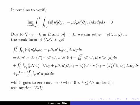
It remains to verify
limε→0
∫ T
0
∫Γδ
(uε1u
ε2∂yv1 − µ∂yu
ε1∂yv1)dxdyds = 0
Due to ∇ · v = 0 in Ω and v2|Γ = 0, we can set ϕ = v(t, x, y) inthe weak form of (NS) to get∫ T
0
∫Γδ
(uε1u
ε2∂yv1 − µ∂yu
ε1∂yv1)dxdyds
= uε, v (T )− uε, v (0)−∫ T0 uε, ∂tv (s)ds
+∫ t0
∫Γδ
(µ∇uε2 · ∇v2 + µ∂xu
ε1∂xv1 − uε
2(uε · ∇)v2 − (uε
1)2∂xv1)dxdyds
+µ1−γ∫ T0
∫Γ u
ε1u1dxds
which goes to zero as ε→ 0 when 0 < δ ≤ Cε under theassumption (ED).
Zhouping Xin

As Temam-Wang, Kelliher did for the non-slip case, we alsohave certain improvement for the previous results:Theorem 5.2 When the slip length αε = o(ε), (ZVL) if andonly if
limε→0
ε
∫ T
0‖∂τu
εn(t)‖2L2(Γδ)dt = 0
for a fixed δ = δ(ε) = o(1) satisfying limε→0µ
δ(ε) = 0.Example: Consider a cylindrically symmetric flow inΩ = x ∈ R3| x1 ∈ R, x2
2 + x23 ≤ 1. Denote by (x1, r, θ) the
cylindric coordinate in Ω. The velocity vector is
uε(t, x) = uε1(t, r)~e1 + uε
θ(t, x1, r)~eθ
where ~e1 = (1, 0, 0)T and ~eθ = 1r (0,−x3, x2)T . Obviously, we
have uε · ~n ≡ 0. So, (ZVL) holds always when the slip length iso(ε).
Zhouping Xin

§6 Asymptotic behavior of boundary layersAs above, we shall only study the case α = µγ . By usingmulti-scale analysis, we conclude:
(1) When γ > 12 , near Γ = y = 0,
uε1(t, x, y) = uB
1 (t, x, yε ) + · · ·
uε2(t, x, y) = εuB
2 (t, x, yε ) + · · ·
with (uB1 , u
B2 )(t, x, η) satisfying
∂tuB1 + uB
1 ∂xuB1 + uB
2 ∂ηuB1 + ∂xP (t, x) = ∂2
ηuB1
∂xuB1 + ∂ηu
B2 = 0
uB1 = uB
2 = 0 on η = 0limη→+∞ uB
1 (t, x, η) = U(t, x)(Prandtl)
Zhouping Xin

(2) When γ = 12 , near Γ = y = 0, the solution uε to (NS)ε
has the same expansion as above, with (uB1 , u
B2 )(t, x, η)
satisfying(Prandtl)
uB2 = 0, uB
1 −∂uB
1∂η = 0 on η = 0
Zhouping Xin

(3) When 0 < γ < 12 , near Γ = y = 0,u
ε1(t, x, y) = µ
12−γuB
1 (t, x, yε ) + o(µ
12−γ)
uε2(t, x, y) = µ1−γuB
2 (t, x, yε ) + o(µ1−γ)
with (uB1 , u
B2 )(t, x, η) satisfying linearized Prandtl
equations.(4) When γ ≤ 0, Boundary layer appears at most at the order
O(ε), and boundary layer profiles satisfy linearized Prandtlequations.
Zhouping Xin

In summary, we observed:When the slip length αε = µγ , γ = 1
2 is critical in determiningthe boundary layer behavior:
I When γ > 12 , the boundary layer profiles satisfy the same
boundary value problem for the nonlinear Prandtlequations as in the non-slip case;
I when γ = 12 , the boundary layer profiles satisfy the
nonlinear Prandtl equations but with a Robin boundarycondition for the tangential velocity;
Zhouping Xin

I when γ < 12 , the boundary layer = O(µ
12−γ), and satisfies a
boundary value problem for linearized Prandtl equations,but with the vorticity
rot uε = O(µ−γ)
being unbounded when 0 < γ < 12 .
I when γ = 0, i.e. the slip length is independent of theviscosity ε, the boundary layer appear in the order O(ε),which yields both of the convection term (uε · ∇)uε and thevorticity rot uε being bounded.
Zhouping Xin

§7 A rigorous justification for an anisotropicviscosity caseConsider the following problem in t, y > 0, x ∈ R : (µ = ε2)
∂tuε + (uε · ∇)uε +∇pε = ε∂2
xuε + µ∂2
yuε
∇ · uε = 0
uε1 − µ
14
∂uε1
∂y = 0, uε2 = 0 on y = 0
uε|t=0 = u0(x, y)
(7.1)
(In this case, the boundary layer profiles satisfy the linearizedPrandtl equations, but the vorticity rot uε = O(µ−
14 ) is
unbounded.)
Zhouping Xin

Suppose that u0 ∈ Hs(Ω) with ∇ · u0 = 0, for a fixed s > 8.(1) Approximate solutions: Let (uε,a, pε,a):
uε,a1 (t, x, y) =
∑3k=0 µ
k4 uI,k
1 (t, x, y) +∑3
k=1 µk4 uB,k
1 (t, x, yε )
uε,a2 (t, x, y) =
∑3k=0 µ
k4 uI,k
2 (t, x, y) + µ34uB,3
2 (t, x, yε )
pε,a(t, x, y) =∑3
k=0 µk4 pI,k(t, x, y)
(7.2)be an approximate solutions satisfying (NS) with errors O(µ).Specially, (uB,j , pB,j)(x, z, t) → 0 exponentially in z → +∞. uI,0
solves the IE with uI,0|t=0 = u0(x, y), pI,1 being a constant. Forall j ≥ 2, (uI,j , pI,j) solves the following linearized Euler systems:
Zhouping Xin
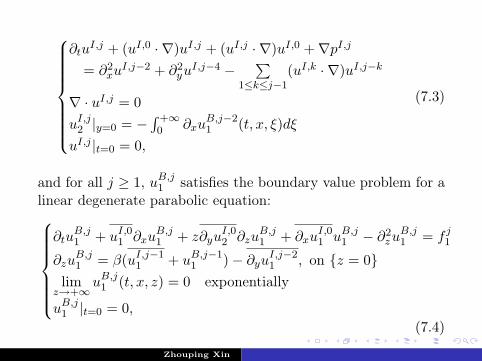
∂tuI,j + (uI,0 · ∇)uI,j + (uI,j · ∇)uI,0 +∇pI,j
= ∂2xu
I,j−2 + ∂2yu
I,j−4 −∑
1≤k≤j−1
(uI,k · ∇)uI,j−k
∇ · uI,j = 0uI,j
2 |y=0 = −∫ +∞0 ∂xu
B,j−21 (t, x, ξ)dξ
uI,j |t=0 = 0,
(7.3)
and for all j ≥ 1, uB,j1 satisfies the boundary value problem for a
linear degenerate parabolic equation:∂tu
B,j1 + uI,0
1 ∂xuB,j1 + z∂yu
I,02 ∂zu
B,j1 + ∂xu
I,01 uB,j
1 − ∂2zu
B,j1 = f j
1
∂zuB,j1 = β(uI,j−1
1 + uB,j−11 )− ∂yu
I,j−21 , on z = 0
limz→+∞
uB,j1 (t, x, z) = 0 exponentially
uB,j1 |t=0 = 0,
(7.4)
Zhouping Xin

where
f j1 =∂2
xuB,j−21 −
j−1∑k=1
[ k2]∑
n=0
zn
n!∂x
(∂n
y uI,k−2n1 uB,j−k
1
)+ uB,k
1 ∂xuB,j−k1
− ∂xp
B,j −j−3∑k=0
[ k2]∑
n=1
zn
n!∂n+1
y uI,k−2n1 uB,j−k
2
−j−1∑k=1
[ k2]+1∑
n=1
zn
n!∂n
y uI,k+2−2n2 ∂zu
B,j−k1
uB,j+22 is given explicitly by
uB,j+22 (t, x, z) =
∫ +∞
z∂xu
B,j1 (t, x, ξ)dξ (7.5)
Zhouping Xin
and for all j ≥ 5, pB,j(t, x, z) is given by
pB,j = −∫ +∞
zf j2 (t, x, ξ)dξ, (7.6)
where
f j2 = ∂2
zuB,j−22 + ∂2
xuB,j−42 − ∂tu
B,j−22
−j−5∑k=0
[ k2]∑
n=0
zn
n!∂n
y uI,k−2n1 + uB,k
1
∂xuB,j−k−22
−j−3∑k=2
[ k2]∑
n=0
zn
n!∂x∂n
y uI,k−2n2 uB,j−k−2
1 −j−5∑k=0
[ k2]∑
n=0
zn
n!∂n+1
y uI,k−2n2 uB,j−k−2
2
−j−3∑k=2
[ k2]∑
n=0
zn
n!∂n
y uI,k−2n2 + uB,k
2
∂zuB,j−k2
Zhouping Xin

(2) Error terms:Let the exact solutions to (NS)ε have expansions:
uε(t, x, y) = uε,a(t, x, y) + µRε(t, x, y)
pε(t, x, y) = pε,a(t, x, y) + µπε(t, x, y).
then (Rε, πε) satisfy:
∂tRε + (uε · ∇)Rε +∇πε − (ε∂2
x + µ∂2y)Rε + (Rε · ∇)uε,a = F ε
∇ ·Rε = 0
Rε2 = 0, Rε
1 − ε14
∂Rε1
∂y = rε(t, x) on y = 0
Rε|t=0 = 0
where F ε, rε are bounded in certain weighted spaces.
Zhouping Xin

(3) Estimate:∫ΩR
ε · (eq)dxdy = 0 ⇒:
ddt‖R
ε(t)‖2L2 + ε‖∂xRε(t)‖2L2 + µ‖∂yR
ε(t)‖2L2
≤ C(‖Rε(t)‖2L2 + ‖F ε(t)‖2L2 + ‖rε(t)‖2L2)−∫ΩRε · (Rε · ∇)uε,adxdy
On the other hand, from ∇ ·Rε and Rε2|y=0 = 0, we get
|∫ΩRε · (Rε · ∇)uε,adxdy| ≤ C1‖Rε(t)‖2L2 + |µ− 1
4∫ΩRε
2Rε1∂ηu
B,11 dxdy|
≤ C1‖Rε(t)‖2L2 + C2µ14 ‖Rε
1(t)‖L2‖∂yRε2‖L2
≤ C2‖Rε(t)‖2L2 + 12ε‖∂xR
ε1‖2L2
Thus, we have‖Rε‖L∞(0,T ;L2) = O(1).
Zhouping Xin

Theorem 7.1 Suppose that the initial data u0 of (IE) belongsto Hs(Ω) for a fixed s > 8. Then, in L∞(0, T ;L2(R2
+)) we have
uε1(t, x, y) = uI,0
1 +∑3
j=1 µj4 (uI,j
1 (t, x, y) + uB,j1 (t, x, y
ε )) +O(µ)
uε2(t, x, y) =
∑3j=0 µ
j4uI,j
2 (t, x, y) + µ34uB,3
2 (t, x, yε ) +O(µ)
pε(t, x, y) =3∑
j=0µ
j4 pI,j(t, x, y) +O(µ)
(7.7)
Zhouping Xin
Working harder with higher order expansions and high Sobolevnorm estimates, we can getTheorem 7.2. Assume that the initial data u0 for (IE) belongsto Hs(Ω) for a fixed s > 18, u02(y = 0, x) = 0, and ∇ · u0 = 0.Then in L∞((0, T )× R2
+), the solution to (7.1) has theasymptotic behavior as in (7.7).
Zhouping Xin

Remark 7.1 (1) The above discussion works for the generalcase µγ with 0 < γ < 1
2 , with the horizontal viscosity beingµ1−2γ while ε being the vertical viscosity. (2) In the same wayas above, we can study the boundary layer behavior for ananisotropic Navier-Stokes equations int > 0,−∞ < x1, x2 < +∞, x3 > 0 as follows:
∂tuε + (uε · ∇)uε +∇pε = ν(∂2
x1+ ∂2
x2)uε + µ∂2
x3uε
∇ · uε = 0uε
3|x3=0 = 0
uεk − µγ ∂u
εk
∂x3= 0, on x3 = 0 (k = 1, 2)
uε|t=0 = u0(x)
with the horizontal viscosity ν being fixed, for any fixed γ ∈ R.(The special case, γ = 0 was studied by Iftimie and Planas in2006.)
Zhouping Xin

§8 Questions and Remarks(1) Rigorous justification of the Prandtl boundary layer
expansion for the non-slip case, even under Oleinik’smonotonic assumption? Or even pressure favorable?
(2) Well-posedness of the Prandtl equations with the Robinboundary condition? Stability? Rigorous justification ofthe boundary layer expansion for the case that the sliplength is equal to the square root of the viscosity?
(3) Can we find a "boundary layer profile" w(t, x, y√ε) such that
uε(t, x, y)− u(t, x, y)− w(t, x,y√ε) = o(1)
holds in L∞(0, T ;H1/2) or in L∞((0, T )× Ω), even withsub-layers and more scales?
(4) Short time well-posedness of Prandtl’s system andnonlinear instability?
Zhouping Xin

THANK YOU!
Zhouping Xin


