Download - Measurement and computation of hydrodynamic …lopez/pdf/jfm_hlm01a.pdfHydrodynamic coupling with an insoluble monolayer 273 Inner (fixed) cylinder Surfactant film Outer (fixed) cylinder

J. Fluid Mech. (2001), vol. 443, pp. 271–292. Printed in the United Kingdom

c© 2001 Cambridge University Press

271

Measurement and computation of hydrodynamiccoupling at an air/water interface with an

insoluble monolayer

By A M I R H. H I R S A1, J U A N M. L O P E Z2

AND R E Z A M I R A G H A I E1

1Department of Mechanical Engineering, Aeronautical Engineering and Mechanics,Rensselaer Polytechnic Institute, Troy, NY 12180, USA

2Department of Mathematics, Arizona State University, Tempe, AZ 85287, USA

(Received 18 October 2000 and in revised form 23 March 2001)

The coupling between a bulk vortical flow and a surfactant-influenced air/waterinterface has been examined in a canonical flow geometry through experiments andcomputations. The flow in an annular region bounded by stationary inner and outercylinders is driven by the constant rotation of the floor and the free surface is initiallycovered by a uniformly distributed insoluble monolayer. When driven slowly, this ge-ometry is referred to as the deep-channel surface viscometer and the flow is essentiallyazimuthal. The only interfacial property that affects the flow in this regime is the sur-face shear viscosity, µs, which is uniform on the surface due to the vanishingly smallconcentration gradient. However, when operated at higher Reynolds number, sec-ondary flow drives the surfactant film towards the inner cylinder until the Marangonistress balances the shear stress on the bulk fluid. In general, the flow can be influencedby the surface tension, σ, and the surface dilatational viscosity, κs, as well as µs. How-ever, because of the small capillary number of the present flow, the effects of surfacetension gradients dominate the surface viscosities in the radial stress balance, and theeffect of µs can only come through the azimuthal stress. Vitamin K1 was chosen forthis study since it forms a well-behaved insoluble monolayer on water and µs is essen-tially zero in the range of concentration on the surface, c, encountered. Thus the effectof Marangoni elasticity on the interfacial stress could be isolated. The flow near theinterface was measured in an optical channel using digital particle image velocimetry.Steady axisymmetric flow was observed at the nominal Reynolds number of 8500. Anumerical model has been developed using the axisymmetric Navier–Stokes equationsto examine the details of the coupling between the bulk and the interface. The nonlin-ear equation of state, σ(c), for the vitamin K1 monolayer was measured and utilizedin the computations. Agreement was demonstrated between the measurements andcomputations, but the flow is critically dependent on the nonlinear equation of state.

1. IntroductionThe dynamics of gas/liquid interfaces play an important role in many fields,

ranging from biomedical applications such as lung surfactant therapy (Grotberg1994) to manufacturing applications such as polyurethane foam stabilization (Snow,Pernisz & Stevens 1998). We are interested in investigating the coupling betweenthe bulk (liquid) flow and the interface in the presence of surface-active materials,surfactants.

272 A. H. Hirsa, J. M. Lopez and R. Miraghaie

The coupling between the liquid subphase and the interface with surfactants hasbeen the subject of numerous studies; many references to this subject are providedby Edwards, Brenner & Wasan (1991). For the most part, these studies have beenrestricted to the Stokes flow (inertialess) limit (e.g. Sacchetti, Yu & Schechter 1993;Schwartz, Knobler & Bruinsma 1994; Chen & Stebe 1996; Stone & Ajdari 1998; John-son & Borhan 1999). While there have been several experimental studies (Warncke,Gharib & Roesgen 1996; Hirsa et al. 1997a) in which the free-surface boundary layeris resolved and theoretical/computational studies of the Navier–Stokes equations(Tsai & Yue 1995; Lopez & Chen 1998; Lopez & Hirsa 1998, 2000), the numberof combined studies directly addressing the coupling with bulk flows that are notrestricted to the Stokes flow are limited (Trygvasson et al. 1992). The experimentsin Trygvasson et al. (1992) only included bulk flow measurements away from theinterface and the free surface boundary layer was not resolved.

The interfacial coupling is a result of the bulk liquid’s viscosity ensuring that thesurfactant film at the interface has the same velocity as the bulk fluid at the interface.The coupling then formally comes about by equating (balancing) the shear stress inthe liquid evaluated at the interface with that of the interface. The interfacial stressis determined from its constitutive relationship. The most widely used constitutiverelation is the Boussinesq–Scriven surface model (Scriven 1960), appropriate for so-called Newtonian interfaces. In such a model, the interfacial stress tensor is composedof an elastic part, due to surface tension, and a viscous part, which is a linear functionof the surface rate of strain. The viscous portion is composed of two parts, a shearand a dilatational component. Note that even for incompressible bulk fluids, theinterfacial velocity will not be (surface) divergence-free in general. Even when theinterface does not exhibit any intrinsic viscosity, the non-divergence-free nature ofthe interfacial velocity has important consequences for the hydrodynamic coupling,particularly with regard to the interfacial advection of surfactants (e.g. Stone & Leal1990; Eggleton, Pawar & Stebe 1999). The resulting stress balance at the interfacethen provides the ‘boundary’ (interface) condition needed to solve the Navier–Stokesequations for the system as a whole.

When the interface is not far from equilibrium, it is reasonable to linearize aboutthe equilibrium state. The majority of studies of interfacial coupling invoke such anassumption, treating the surface tension gradient and surface viscosities (if applicable)as constants. Eggleton et al. (1999) have shown, however, that even in the Stokes flowlimit, the hydrodynamic coupling is very sensitive to nonlinearities in the equation ofstate, relating the surface tension to the thermodynamic state of the interface (throughthe surfactant concentration). With bulk flows that are not restricted to the Stokeslimit, one can expect the interface to be more readily driven away from uniformsurfactant coverage, making the precise form of the equation of state crucial for acorrect description of the coupled system.

In the present study we test the appropriateness of a Newtonian surface constitutiverelation for vitamin K1, which forms an insoluble monolayer on water (Gaines1966). For the range of concentrations used, we have determined that the surfaceshear viscosity is negligible, and for the range of capillary number considered theMarangoni stress dominates any contribution from the viscous resistance to surfacedilations. So, the only issue to address is whether the nonlinear equation of statewhen incorporated into the constitutive relation gives the correct hydrodynamics.The vitamin K1 monolayer is well behaved (Weitzel, Fretzdorff & Heller 1956), inthe sense that measurements of the ‘equation of state’ obtained through the standardtechnique of surface compression in a Langmuir trough give essentially identical

Hydrodynamic coupling with an insoluble monolayer 273

Inner (fixed)cylinder

Surfactantfilm

Outer (fixed)cylinder

Gas

Liquid

Rotatingfloor

dz

ri

ro

Ω

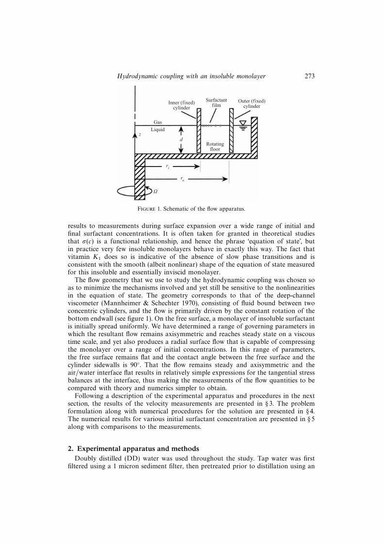
Figure 1. Schematic of the flow apparatus.

results to measurements during surface expansion over a wide range of initial andfinal surfactant concentrations. It is often taken for granted in theoretical studiesthat σ(c) is a functional relationship, and hence the phrase ‘equation of state’, butin practice very few insoluble monolayers behave in exactly this way. The fact thatvitamin K1 does so is indicative of the absence of slow phase transitions and isconsistent with the smooth (albeit nonlinear) shape of the equation of state measuredfor this insoluble and essentially inviscid monolayer.

The flow geometry that we use to study the hydrodynamic coupling was chosen soas to minimize the mechanisms involved and yet still be sensitive to the nonlinearitiesin the equation of state. The geometry corresponds to that of the deep-channelviscometer (Mannheimer & Schechter 1970), consisting of fluid bound between twoconcentric cylinders, and the flow is primarily driven by the constant rotation of thebottom endwall (see figure 1). On the free surface, a monolayer of insoluble surfactantis initially spread uniformly. We have determined a range of governing parameters inwhich the resultant flow remains axisymmetric and reaches steady state on a viscoustime scale, and yet also produces a radial surface flow that is capable of compressingthe monolayer over a range of initial concentrations. In this range of parameters,the free surface remains flat and the contact angle between the free surface and thecylinder sidewalls is 90. That the flow remains steady and axisymmetric and theair/water interface flat results in relatively simple expressions for the tangential stressbalances at the interface, thus making the measurements of the flow quantities to becompared with theory and numerics simpler to obtain.

Following a description of the experimental apparatus and procedures in the nextsection, the results of the velocity measurements are presented in § 3. The problemformulation along with numerical procedures for the solution are presented in § 4.The numerical results for various initial surfactant concentration are presented in § 5along with comparisons to the measurements.

2. Experimental apparatus and methodsDoubly distilled (DD) water was used throughout the study. Tap water was first

filtered using a 1 micron sediment filter, then pretreated prior to distillation using an


Surface pressure (dyn cm−1)

Water sample 0 h 1 h 2 h 3 h Resistivity (MΩ cm)

Unseeded DD 0.10 0.10 0.16 0.16 6.6Seeded DD 0.10 0.10 0.10 0.10 6.7Commercial D 0.10 0.16 0.16 0.16 6.3HPLC 0.16 0.16 0.32 0.64 5.6

Table 1. Surface pressure of various water samples of the indicated age, obtained by rapidcompression. Note that the pH of all samples tested was indistinguishable and in the range 6.5–7.0,as expected for pure water.

organic removal filter (Barnstead, model D8904) and an ion removing filter (Barnstead,D8921). Following the pretreatment, the water was first distilled in a Stokes distiller(Water Distillers Inc., 171-E) and then in a glass second distiller (Corning, AG-1B).The water was handled only using HF acid-etched glass containers and dispensedfrom a Teflon squeeze bottle. The surface tension of the DD water was identical to theexpected value (Weast 1980) within the experimental uncertainty (±0.05 dyn cm−1).Table 1 shows a comparison of the surface pressure π (surface tension of the cleanestwater minus the surface tension of the water in question) as a function of the ageof the surface for the present DD water, HPLC-grade water (Aldrich, catalogueNo. 27073-3), and commercial distilled water (Poland Springs). The surface pressurewas measured in a Langmuir trough, described below, immediately following a rapidcompression (10 : 1 compression in under 60 s). This was done in order to closely packthe residual surfactant molecules, making their presence more easily detectable beforethey can desorb from the interface. The relative purity of the present DD water isevident from table 1. For reference, the measured resistivity and pH of each watersample is also included in the table.

The interfacial property measurements for the vitamin K1 monolayer on waterwere performed using established techniques. The surface tension was measured usinga Wilhelmy plate and electrobalance (Nima, PS4). Filter paper (Nima) was used asthe plate to ensure complete wetting. Surface tension measurements were made asa function of surfactant concentration in a Langmuir trough constructed of Teflon.Vitamin K1 (Aldrich, 28740-7) was diluted with 99+% pure hexane (Aldrich, 13938-6)and spread using a glass microsyringe (Hamilton, 14813112). The cleanliness of theLangmuir trough and the purity of the hexane were established in the trough priorto measurements of the equation of state. The equation of state for the vitaminK1 monolayer, at temperature 23 ± 1 C, is shown in figure 2(a). A close-up of thedata is shown in figure 2(b). The error in the measurement of surface tension hasbeen estimated to be less than ±0.05 dyn cm−1 and the error in the measurement ofsurfactant concentration is less than ±5%.

The other interfacial properties required for the interfacial stress balance are thesurface shear viscosity, µs, and surface dilatational viscosity, κs. Established techniquesare available for the measurement of µs. The surface shear viscosity for a vitamin K1

monolayer was measured using a standard deep-channel surface viscometer (Edwardset al. 1991). This surface viscometer was constructed of stainless steel and haddimensions similar to that introduced by Mannheimer & Schechter (1970). For therange of concentration used in this study (less than 1.5 mg m−2), vitamin K1 exhibitedno detectable surface shear viscosity. The deep-channel surface viscometer is sensitive


74

72

70

68

66

640 0.25 0.50 0.75 1.00 1.25 1.50

c (mg m–2)

(a)

σ (

dyn

cm–1

)

72.4

72.2

72.0

71.80 0.2 0.4 0.6 0.8 1.0 1.2

c (mg m–2)

(b)

Figure 2. (a) Equation of state, σ(c), for a vitamin K1-water system measured using a Langmuirtrough (symbols) together with a nonlinear curve fit given by (4.14); (b) close-up of (a).

down to approximately 10−4 g s−1 (surface Poise), therefore the dimensionless surfaceshear viscosity (µs/µro, where µ is viscosity in the bulk and ro is the outer radius,nominally 10 cm) is less than 10−3 and thus neglected. The surface dilatational viscosityhas not yet been measured consistently with any two different experimental techniquesfor any surfactant (Edwards et al. 1991). However, for the flows investigated here, thecapillary number is so low that surface dilitational effects are negligible compared tothe surfactant Marangoni stress (Lopez & Hirsa 2000).

Figure 3 shows a schematic of the optical channel in which the velocity wasmeasured. The floor of the channel consists of an optical window, which is rotatedby a computer controlled stepping motor. The water is contained by a cast acryliccylinder bonded to the glass floor. The inner and outer cylinders consist of 2.5 cm highcast acrylic tube, with radii ri = 7.62±0.01 cm and ro = 9.82±0.01 cm. The thickness ofthe (stationary) outer cylinder was minimized (≈ 0.3 cm) to reduce optical distortion.The stationary cylinders were press-fitted into grooves precision machined in the coverwhich held them at 0.0076 ± 0.005 cm above the rotating floor. The tolerance in thegap (±0.005 cm) was primarily due to the finite wobble of the rotating floor. A groovewas machined on each cylinder at 1.1 cm from the bottom (not shown in figure 1)in order to fix the location of the contact line. Paraffin from a hexane solution wasdeposited in the groove to ensure that the water wetted the cylinder walls only up tothe bottom of the groove. Thus, by filling water in the container to a depth of 1.1 cm,a 90 contact angle was achieved resulting in a flat air/water interface in the 2.2 cmwide region between the cylinders. The depth-to-gap ratio, Λ = d/(ro − ri) = 0.5 andthe radius ratio ri/ro = 0.776.

The velocity measurements were primarily performed in the meridional plane (r, z),see figure 3, where the radial and vertical velocity components, u and w, were obtainedand the azimuthal vorticity, η, determined. Due to the relatively high magnificationof the DPIV imaging system (as high as 63 pixels mm−1), it was necessary to avoidthe optical distortion that would occur by viewing the illuminated meridional planethrough the rotating container. The variations in the thickness and radius of therotating container can result in time-dependent refraction. To avoid viewing throughthe rotating cylinder, a periscope setup was devised to permit viewing the meridionalplane from between the fixed outer cylinder and the rotating cylinder. As depictedin figure 3, a right prism was partially submerged in the water outside of the fixed


Rotatingcontainer

Rotatingfloor

DPIVcamera

Opticalpath Partially

submergedprism

Laser sheet(meridional plane)

Ω

Stationaryinner and

outer cylinders

Figure 3. Schematic of the optical channel showing the stationary cylinders, rotating container, andthe optical setup. The prisms were only used for measurements in the meridional plane which isilluminated by a vertical laser sheet.

outer cylinder and held stationary. A second right prism was held stationary abovethe partially submerged prism to allow horizontal viewing with the camera. For themeasurements in the meridional plane, a vertical laser light sheet with a thicknessof 0.1 cm was directed upward through the optical floor. For measurements in theplane of the surface (z = d), a horizontal light sheet with a thickness of less than0.05 cm was directed radially inward. The illuminated horizontal plane was imagedfrom beneath the channel using a mirror at 45 held stationary below the rotatingoptical floor.

The technique of digital particle image velocimetry (DPIV) utilized here has beenpresented elsewhere (Logory, Hirsa & Anthony 1996; Hirsa et al. 1997b), as has themethod of boundary-fitted DPIV (Hirsa, Vogel & Gayton 2001; Vogel et al. 2001) usedfor resolving the interfacial velocity and vorticity in meridional plane measurements,and so will be not be repeated here. However, the preparation of the seeded waterrequired special attention to achieve the requisite level of purity and is described herein some detail. Polystyrene particles stabilized with surface-bound sulphate groupswere used for this experiment. For high magnification measurements (63 pixels mm−1)in the meridional plane, 3 micron particles (Aldrich, 45941-0) were utilized. Formeasurements in the surface plane (22 pixels mm−1), particles of 11.9 micron diameter(Aldrich, 45942-9) were used. Both of these particles can be thoroughly cleanedwithout causing them to form clusters. The seeding particles, which were received in awater suspension were first rinsed with HPLC isopropyl alcohol (2-propanol; Aldrich,27049-0). This was accomplished by withdrawing a volume of the particle suspension(10% solid) and depositing it in a test tube partially filled with the isopropyl alcohol;0.2 ml of the 3 micron or 0.5 ml of the 11.9 micron particle suspension was used. Thetest tube was then centrifuged and the liquid was aspirated leaving the wet seedingparticles at the bottom. Fresh isopropyl alcohol was then added to the test tube and


the contents were thoroughly shaken by submersion in an ultrasonic cleaner bath. Thetest tube was then centrifuged and the isopropyl alcohol was aspirated. The cleaningprocess (solvent addition, ultrasonic shaking, centrifuge, followed by aspiration) wasthen repeated twice with HPLC methanol (Aldrich, 27047-4) and four times with DDwater. The cleaned particles were added to a 4 l conical flask filled with DD water.As a final step in removing surfactants from the seeded water, pure nitrogen bubbles(generated from liquid nitrogen boil-off) were introduced from a Pyrex gas dispersiondisc (Fisher Scientific, 11-137F). Residual surfactants are adsorbed on the nitrogenbubbles (e.g. see Scott 1975) and brought to the surface where they are continuouslyaspirated and fresh DD water was added at a rate of 1 l h−1 to maintain a constantwater level. This process was continued for at least 1 hour. The resulting water wasseeded with less than 4 p.p.m. (by volume and mass) of clean polystyrene particles.Surface pressure measurements of the seeded water, presented in table 1, demonstratethe effectiveness of the cleaning process, including the bubbling with nitrogen gas.Ultimately, however, the success of the cleaning process was evaluated in the opticalchannel via measurements of the radial surface velocity at the interface without adeposited monolayer.

3. Results of velocity field measurementsThe interfacial flow measurements were performed with the floor rotating at Ω =

0.843 rad s−1. The resulting Reynolds number Re = Ωr2o/ν = 8.5× 103, where ν is the

kinematic viscosity (9.35×10−3 cm2 s−1 for water at 23 C). The capillary number, Ca =µΩro/σo = 10−3, where µ is the dynamic viscosity in the bulk (9.33× 10−3 g cm−1 s−1)and σo = 72.4 dyn cm−1 is the surface tension for clean water at this temperature.

Since strong secondary flow requires relatively large Re (Lopez & Hirsa 1998), astability study was first undertaken to determine the margin of stability at the presentReynolds number. The flow in a meridional plane was measured with DPIV at thelocation z/d = 0.5 and x = (r−ri)/(ro−ri) = 0.25. This location in the core of the flowwas selected because the velocity is adequately large to avoid excessive noise from theDPIV analysis, and is outside of the wall boundary layers where disturbances tendto be dampened. Figure 4 shows the root-mean square of the vertical velocity, wrms,non-dimensionalized with Ωro. Measurements taken on three different days (labelledSeries 1–3) are shown for Reynolds number between 4000 and 14 000 (by varying Ω).The expected level of noise from the DPIV system, computed based on uncertaintyof 0.2 pixels for velocity squared (0.1 pixels for velocity) is shown for reference. Com-parison between the measured and the expected noise level illustrates that the flow isessentially steady, and hence axisymmetric, for Re up to about 12 000. For Re = 8500,the value used for the interfacial measurements, the flow reached an axisymmetricsteady state following a constant-acceleration start-up (for 27 s from rest) withinabout 100 s. This is the diffusive time scale through the depth of the bulk fluid.

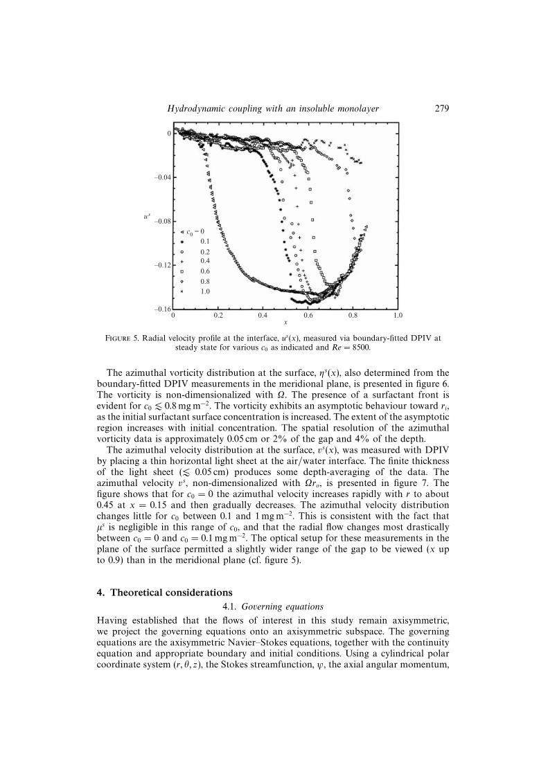
The radial velocity distribution at the interface (z = d), us(x), obtained viaboundary-fitted DPIV measurements in a meridional plane, is shown in figure 5for c0 up to 1.0 mg m−2. The velocity data are non-dimensionalized with Ωro andshown as a function of the dimensionless gap, x. In the absence of a depositedmonolayer (c0 = 0), the surface is clean except for a narrow region near the innercylinder. Residual contamination tends to accumulate on the interface near the innercylinder due to the action of secondary flow in the bulk. The flow field, including thesecondary flow in the bulk, is described in some detail in § 5. The residual contami-nation diminishes the radially inward velocity faster than would otherwise occur in an


0.004

0.003

0.002

0.001

04000 8000 12000 16000

Re

wrms

Series 1Series 2Series 3DPIV noise

Figure 4. Root-mean-square of the vertical velocity, scaled by Ωro, at the point (r−ri)/(ro−ri) = 0.25,z/d = 0.5 measured on three separate days (Series 1–3) over a range of Re, together with the noiselevel from the DPIV system (dashed line).

absolutely clean medium. The contaminated region is approximately 0.2 cm wide orless than 10% of the gap. The extent of the velocity measurements in the meridionalplane was limited in the region x → 1 by the optical distortion due to the curvatureof the outer cylinder near ro. Data in this plane will only be presented up to x = 0.85.For the c0 = 0 case, the peak interfacial velocity in the radial direction is −0.145 andoccurs at approximately x = 0.6. The spatial resolution of these measurements, basedon the final cross-correlation window (16 pixels), is 0.025 cm or approximately 1% ofthe gap and 2% of the depth. The resolution of the measurements, which amountsto spatial filtering, is especially important when comparing the experimental resultsto computations (see § 5).

As part of the boundary-fitted DPIV technique utilized for velocity measurementsin the meridional plane, the location of the free surface is determined. The measure-ments showed that the extent of surface deformation, from the highest point to thelowest, was less than 50 microns. The accuracy of this measurement is approximately±10 microns, corresponding to approximately 0.5 pixel. Thus, the surface is found tobe relatively flat, with the maximum departure from the undisturbed surface of only0.2% of the depth. The measured deformation is consistent with the deformationestimated from the Froude number, Fr = Ω2r2

o/gd of order 10−2 for Re = 8500.The measured radial velocity distribution is in qualitative agreement with earlier

calculations for a similar geometry and Re but for a different surfactant system(Lopez & Hirsa 2000). Flow calculations for the vitamin K1 case are presented in thefollowing sections. Figure 5 shows that with increasing initial concentration of thevitamin K1 monolayer, the radial flow diminishes as the monolayer is accumulatedtoward the inner cylinder. A slight increase in the magnitude of the peak velocity canbe observed for finite c0 up to 0.4. It is apparent that the radial velocity diminishesfor c0 > 0.8 mg m−2 and the vitamin K1 monolayer covers the entire measurementregion.


0

–0.04

–0.08

–0.12

–0.160 0.2 0.4 0.8

x

us

c0 = 0

0.6 1.0

c0 = 0.1

c0 = 0.2c0 = 0.4

c0 = 0.6

c0 = 0.8c0 = 1.0

Figure 5. Radial velocity profile at the interface, us(x), measured via boundary-fitted DPIV atsteady state for various c0 as indicated and Re = 8500.

The azimuthal vorticity distribution at the surface, ηs(x), also determined from theboundary-fitted DPIV measurements in the meridional plane, is presented in figure 6.The vorticity is non-dimensionalized with Ω. The presence of a surfactant front isevident for c0 . 0.8 mg m−2. The vorticity exhibits an asymptotic behaviour toward ri,as the initial surfactant surface concentration is increased. The extent of the asymptoticregion increases with initial concentration. The spatial resolution of the azimuthalvorticity data is approximately 0.05 cm or 2% of the gap and 4% of the depth.

The azimuthal velocity distribution at the surface, vs(x), was measured with DPIVby placing a thin horizontal light sheet at the air/water interface. The finite thicknessof the light sheet (. 0.05 cm) produces some depth-averaging of the data. Theazimuthal velocity vs, non-dimensionalized with Ωro, is presented in figure 7. Thefigure shows that for c0 = 0 the azimuthal velocity increases rapidly with r to about0.45 at x = 0.15 and then gradually decreases. The azimuthal velocity distributionchanges little for c0 between 0.1 and 1 mg m−2. This is consistent with the fact thatµs is negligible in this range of c0, and that the radial flow changes most drasticallybetween c0 = 0 and c0 = 0.1 mg m−2. The optical setup for these measurements in theplane of the surface permitted a slightly wider range of the gap to be viewed (x upto 0.9) than in the meridional plane (cf. figure 5).

4. Theoretical considerations4.1. Governing equations

Having established that the flows of interest in this study remain axisymmetric,we project the governing equations onto an axisymmetric subspace. The governingequations are the axisymmetric Navier–Stokes equations, together with the continuityequation and appropriate boundary and initial conditions. Using a cylindrical polarcoordinate system (r, θ, z), the Stokes streamfunction, ψ, the axial angular momentum,


24

20

16

12

8

4

0

–40 0.2 0.4 0.8

x

η s

c0 = 0.1

0.6 1.0

c0 = 0.2c0 = 0.4

c0 = 0.6c0 = 0.8c0 = 1.0

Figure 6. Azimuthal vorticity profile at the interface, ηs(x), measured via boundary-fitted DPIV atsteady state for various c0 as indicated and Re = 8500.

0.5

0.4

0.3

0.2

0.1

0 0.2 0.4 0.8x

v s c0 = 0

0.6 1.0

c0 = 0.1c0 = 0.2c0 = 0.4c0 = 0.8c0 = 1.0

Figure 7. Azimuthal velocity profile at the interface, vs(x), measured via DPIV at steady state forvarious c0 as indicated and Re = 8500.

α, and the azimuthal component of vorticity, η, the non-dimensional velocity vectoris

u = (u, v, w) =

(−1

r

∂ψ

∂z,α

r,1

r

∂ψ

∂r

), (4.1)


and the corresponding vorticity vector is

∇× u =

(−1

r

∂α

∂z, η,

1

r

∂α

∂r

). (4.2)

The use of ψ and α is convenient in axisymmetric swirling flows; contours of ψ inan (r, z)-plane depict the streamlines of the flow, and contours of α in that planedepict the vortex lines. Recall that vortex lines cannot begin or end at a stationarysolid wall, they must be tangential to it, and at a flat stress-free (e.g. clean) gas/liquidinterface the vortex lines are normal to it.

Using ro as the length scale and 1/Ω as the time scale, the non-dimensionalizedaxisymmetric Navier–Stokes equations are

Dα

Dt=

1

Re∇2∗α, (4.3)

Dη

Dt+η

r2

∂ψ

∂z− 1

r3

∂α2

∂z=

1

Re

(∇2η − η

r2

), (4.4)

where

∇2∗ψ = −rη, (4.5)

D

Dt=

∂

∂t− 1

r

∂ψ

∂z

∂

∂r+

1

r

∂ψ

∂r

∂

∂z, (4.6)

∇2 =∂2

∂z2+∂2

∂r2+

1

r

∂

∂r, (4.7)

and

∇2∗ =

∂2

∂z2+∂2

∂r2− 1

r

∂

∂r. (4.8)

The boundary conditions on the solid boundaries are no-slip, i.e. the normal andtangential derivatives of ψ vanish; α = 0 on the stationary cylinder walls and α = r2

on the rotating floor. The azimuthal vorticity η on the solid boundaries is determinedby evaluating (4.5) on the boundaries once ψ is known. On the air/water interface,being a material surface, ψ is continuous with its value on the sidewalls, which we setto zero without loss of generality. Consistent with the measurements, we shall assumethat the interface is flat, and hence the contact angle at the air/water/solid contactline is 90. The conditions for α and η on the interface remain to be specified.

Our treatment of the interface considers the Boussinesq–Scriven surface fluidmodel for a Newtonian gas/liquid interface (Boussinesq 1913; Scriven 1960; Aris1962; Slattery 1990), where the surface stress tensor is

T s = σIs + Ss = (σ + (κs − µs)divsus)Is + 2µsDs, (4.9)

and the viscous part of the surface stress tensor, Ss, is described as a linear functionof the surface rate of deformation tensor

2Ds = ∇sus · Is + Is · (∇sus)T . (4.10)

In this constitutive equation, κs is the surface dilatational viscosity, µs is the surfaceshear viscosity, σ is the thermodynamic (equilibrium) surface tension, us is the surfacevelocity vector, divs is the surface divergence operator, ∇s is the surface gradientoperator, and Is is the tensor that projects any vector onto the interface (for theflat interface considered in this study, Is is the identity). This formulation allows thesurface viscosities to vary with the surfactant concentration; this is important when


considering certain surfactants, such as hemicyanine (Lopez & Chen 1998; Hirsa1998, 2000). We also allow for a nonlinear equation of state, σ(c). A description ofthe general formulation is given in Lopez & Hirsa (2000).

Due to the vanishingly small measured values of µs for the range of surfactantconcentrations encountered in the experiments and the relatively small Ca, µs and κs

may be neglected for this study. The azimuthal stress balance, written in terms ofnon-dimensional α, then reduces to

∂α

∂z= 0, (4.11)

which says that vortex lines meet the air/water interface normally. The radial stressbalance, in terms of non-dimensional ηs reduces to

ηs =1

Ca

∂σ

∂r, (4.12)

which says that the radial stress balance is solely due to surface tension gradients,i.e. the (surfactant) Marangoni stress. Note that σ denotes the non-dimensionalizedsurface tension, defined below.

Since the surface tension, σ, is a function of the surfactant concentration c, we needto solve an active scalar advection–diffusion equation for c on the interface:

∂c

∂t=

1

r

∂

∂r

(c∂ψ

∂z

)+

1

Pes

(∂2c

∂r2+

1

r

∂c

∂r

), (4.13)

where Pes = Ωr2o/D

s is the surface Peclet number and Ds is the surface diffusion of thesurfactant; Ds is estimated to be of order 10−5 cm2 s−1 for typical surfactants (Agrawal& Neuman 1988). In our experiments, Ωr2

o = 81.3 cm2 s−1, and in the computationswe use Pes = 105. At the contamination front, the large gradients in concentrationlead to a large production in surface azimuthal vorticity, resulting in a spike in ηs

whose width scales with 1/√Pes.

The nonlinear equation of state used in the computations is a fit to the experimen-tally measured surface tension of vitamin K1 on a water substrate, as detailed in § 2.Figure 2 show this nonlinear fit along with the experimental measurements. The fithas the form

σ(c) = σ0σ(c) =a2 + a3c+ a4c

2

1 + exp (a0a1 − a1c)+

a5 + a6c2

1 + exp (a1c− a0a1), (4.14)

where σ0 = 72.4, a0 = 1.108, a1 = 32.37, a2 = 20.11, a3 = 97.04, a4 = −45.9, a5 = σ0,and a6 = −0.15; note σ0 has the unit dyn cm−1 (mN m−1).

4.2. Numerical technique

Due to the nonlinear coupling between the bulk flow and the boundary conditions,an explicit time integration is implemented. We begin by discretizing in space usingsecond-order centred differences. Equations (4.3) and (4.4) then have the form

dαi,jdt

= RHS1(α, ψ), (4.15)

anddηi,jdt

= RHS2(η, α, ψ). (4.16)

The computational domain is r ∈ [ri/ro, 1], z ∈ [0, d/(ro − ri)] with r = ri/ro + i(ro −ri)/ronr for i ∈ [0, nr], and z = jd/ronz for j ∈ [0, nz]. Note that results will be


presented in terms of x = (r − ri)/d. All the computations were done using nr = 600,nz = 300, δt = 2 × 10−4, d/(ro − ri) = 0.5, and ri/ro = 0.776. This fine resolutionis more than sufficient to produce grid-independent results for the bulk flow. Theneed for such fine resolution stems from the use of a relatively high Pes = 105, aswhen a surfactant front forms for a range of parameters, the azimuthal vorticity atthe interface has a sharp spike that necessitates the fine resolution. The usual testswhere the grid spacing and time-step are halved have been performed, and it hasbeen determined that the resolution used gives asymptotically converged results.

Starting from the initial conditions, the interior values of αi,j and ηi,j (i ∈ [1, nr − 1]and j ∈ [1, nz − 1]) are evolved forward in time using a second-order predictor–corrector scheme. Denoting the current time by superscript k, the predictor stage bysuperscript ∗, and the next (corrected) stage by k + 1, we first evaluate

α∗i,j = αki,j + δtRHSk1 , (4.17)

and

η∗i,j = ηki,j + δtRHSk2 . (4.18)

At this stage, we need to solve the elliptic equation (4.5) for ψ∗ with the interiorpoints for η∗ just computed. Then, the surfactant concentration is advected by thisstreamfunction. So (4.13) is solved for c∗ with ψ∗, and the boundary conditions∂c/∂r = 0 at r = ri/ro and 1 (thus conserving total surfactant on the interface). Thisevolution is also done by the predictor–corrector scheme. One needs to do the fulltwo stages to get from ck to c∗∗ to c∗, both stages using ψ∗. With c∗(r), we evaluate∂σ(c∗(r))/∂r. The boundary conditions for α∗ and η∗ are then evaluated. On theno-slip boundaries, this is straightforward. For the interface, we solve for α by usingone-sided differences to discretize (4.11). Equation (4.12) gives ηs directly from thesurface tension gradient. We now have everything (α, η, ψ, and c) at the predictorstage, and can repeat the whole process to obtain the corrector stage. We evolve αand η using

αk+1i,j = 0.5(αki,j + α∗i,j + δtRHS∗1 ), (4.19)

and

ηk+1i,j = 0.5(ηki,j + η∗i,j + δtRHS∗2 ). (4.20)

5. Numerical results and discussion5.1. Comparison of clean surface measurements and computations

The computed profiles of the radial and azimuthal velocity on the surface for the cleancase (c0 = 0) are presented in figures 8(a) and 8(b), respectively. The measured velocityprofiles are also plotted in the figures. The results show good agreement between themeasurements and the calculations for the clean interface except for a narrow regionnear the inner cylinder (x = 0) where residual surfactants which are inevitable in anyexperiment diminish the radial velocity and, in turn, alter the azimuthal velocity. Forcomparison, the computed profiles for a case with a minute amount of vitamin K1

initially on the surface (c0 = 0.05 mg m−2) are also shown. Figure 8(a) shows thatthe measured radial velocity becomes zero at x = 0.1, compared to the computedc0 = 0.05 mg m−2 case in which the radial velocity diminishes at x = 0.2. The plotsillustrate that the residual surfactants in the experimental flow, in general expectedto be soluble, are comparable to less than 0.05 mg m−2 of vitamin K1 monolayerspread uniformly on the surface. The error in the velocity measurements, estimated


0.5

0.4

0.3

0.2

0.1

0 0.2 0.4 0.8x

v s

0.6 1.0

(b)

0 0.2 0.4 0.8

us

0.6 1.0

(a)0

–0.04

–0.08

–0.12

–0.16

Figure 8. Profile of (a) radial velocity at the interface, us(x), and (b) azimuthal velocity at theinterface, vs(x), at steady state for Re = 8500: measurements of the clean interface (symbols),computed profiles for c0 = 0.0 (solid) and c0 = 0.05 (dashed).

to be ±2% of full scale, can account for some of the observed differences betweenthe measurements and the computed profiles, especially in the outer region (x > 0.6).More importantly, the resolution of the measurements is one order of magnitude lessthan that of the computations, and as a result the measured velocity data representa finite degree of depth averaging (2–4% depth averaging for the measurements cf.node spacing of 0.3% of the depth in the computations). Another factor that maycontribute to the discrepancies between the measurements and computations is thevariation in Reynolds number due to viscosity changes caused by uncertainty inthe temperature. The uncertainty in the temperature, ±1C, represents a variationof ±2.2% in Reynolds number. Considering these factors, the overall agreementbetween the measured surface velocity components and the computations is good.


(a) c0 = 0

(b) c0 = 0.1

(c) c0 = 0.2

(d ) c0 = 0.4

(e) c0 = 0.8

Figure 9. Contours of ψ (left), η (middle), and α (right), at steady state with Re = 8500 and initialuniform distribution of vitamin K1 on the interface, c0. The dashed lines are negative and solidlines are positive contours of η.

5.2. Coupling between the interface and bulk flow

The computed bulk flow for a range of initial surfactant concentrations, starting froma clean surface (c0 = 0) is shown in figure 9. Contours of the streamfunction, ψ,azimuthal vorticity, η, and angular momentum, α, are presented. The bulk secondaryflow which drives the interfacial flow is apparent in the contours of ψ. This bulk flowoverturns in the counter-clockwise direction. The boundary layers on the (stationary)inner and outer cylinders, as well as the relatively strong boundary layer on therotating bottom, are evident from the η contours. As expected for the clean case, theazimuthal vorticity decreases to zero at the surface (z = d) in a thin region. Notethat at the surface, this component of vorticity is the radial shear stress ∂u/∂z. Theη contours near the interface indicate that the presence of the boundary layer onthe inner cylinder is evident on the surface for x up to approximately 0.06. Furtherevidence of the deceleration of the radial inflow is the small recirculation zone atthe corner where the surface meets the inner cylinder. This is consistent with the


measurements of u at the interface, which diminished rapidly at x = 0.06, indicatingthat residual surfactants covered the surface up to approximately x = 0.1 for thecase with no added surfactants (c0 = 0). This suggests that even a minute amount ofresidual surfactant can remain spread in that region.

For finite c0, figure 9 shows that a boundary layer forms at the air/water interface.For c0 < 0.8 mg m−2 the secondary flow near the surface is strong enough to compressthe monolayer towards the inner cylinder and clean a portion of the surface, forcingthe leading edge of the free-surface boundary layer to the left. The meridional bulkflow, as depicted by the streamlines, slows down considerably beneath the surfaceboundary layer (in fact u→ 0 as z → d), but is accelerated compared to the clean casebeneath the portion of the surface that has been swept clean of the surfactant. This isin agreement with the measurements (see figure 5). The state of the interface changesthe entire bulk flow structure, not just in the neighbourhood of the interface. This ismost notable in the boundary layer structure on the inner cylinder all the way downto the rotating bottom. Also, the change imparted to the bulk meridional circulationby the presence of surfactants has a pronounced influence on the way the vortex lines(contours of α) are advected into the interior; their axial gradients directly affect η inthe interior (through the (−1/r3)∂α2/∂z term in (4.4)). This then directly feeds backinto the meridional flow (ψ) through (4.5). So the nonlinear coupling between theinterface and the bulk flow is manifest throughout the entire flow field.

The initial condition at the interface is of a uniform monolayer of concentrationc0. So, initially, ∂σ/∂r = 0 and surfactants are swept radially inwards by the bulkradial flow at the interface. Two things happen as the monolayer is swept inwards:(i) a concentration gradient develops, ∂c/∂r < 0, and (ii) the concentration buildsup at smaller r so that the part of the equation of state that is in play has largergradients, ∂σ/∂c < 0. For small c0, the surfactants can be swept until the combination(∂σ/∂c)∂c/∂r, i.e. the Marangoni stress, is large enough to resist any further build-upof surfactants. At this point, a contamination front is established. In figure 10 areplotted at steady state the concentration profiles for Re = 8500 over a range of c0. Forvery small c0 (∼ 0.05 mg m−2), almost the entire surface is swept clean of surfactants;for larger c0 the extent of the cleansing is diminished, and for c0 > 0.8 mg m−2 thereis no cleaning, although the bulk radial flow is still able to compress the monolayerto some degree. The location of the contamination front depends critically on thenonlinear form of the equation of state and the strength of the bulk radial flow atthe interface (essentially measured by Re and Λ = d/(ro − ri)). Near the interface,us generally increases with increasing Re and decreasing Λ. The uncertainty in theexperimental determination of σ(c), particularly in the measurement of c (±5%error), is enough to account for the differences between the measured and computedflows. Another factor to consider when comparing the experiments with a depositedmonolayer and the calculations is the small, but finite, amount of residual surfactantin the bulk in the experiment that may interact with the vitamin K1 monolayer.The effect of a soluble surfactant on the equilibrium surface tension of an insolublemonolayer has been studied in the past (e.g. see Sundaram & Stebe 1996). However,much less is known about the soluble/insoluble interaction in flowing systems.

At the contamination front, there is essentially a shock in c (it is not a discontinuitydue to the finite surface diffusivity, Pes), and this leads to a large spike in the surfaceshear stress, as seen in the profiles of ηs (figure 11). The width of this spike scales with1/√Pes. From the figure, it can be seen that behind the spike where the monolayer

resides, ηs relaxes to a distribution corresponding to ηs for c0 > 0.8, i.e. the ηs of anycase with no surface cleaning. Also, behind the front, us → 0 (see figure 12a). However,


1.2

1.0

0.8

0.6

0.4

0.2

0 0.2 0.4 0.8x

c

0.6 1.0

0.05

0.1

0.2

0.4

0.60.8

1.0

Figure 10. Computed profiles of surfactant concentration, c(x),for c0 as indicated, at steady state for Re = 8500.

0 0.2 0.4 0.8x

η s

0.6 1.0

0.05

0.1

0.20.4

0.6

0.8, 1.0

150

125

100

75

50

25

Figure 11. Computed profiles of azimuthal vorticity at the interface, ηs(x),for c0 as indicated, at steady state for Re = 8500.

in the azimuthal direction, since the flow is axisymmetric, there are no concentrationgradients for any c0, and the surface azimuthal velocity, vs, for inviscid surfactantsystems is not directly aware of the presence of surfactants. This is illustrated infigure 12(b), where vs profiles for a range of c0 ∈ [0.0, 1.0] are plotted; these profilesare little affected by c0, consistent with the measurements.

Typically when the Marangoni stress is dominating, the interface is thought of asimmobile, acting as a no-slip surface. But this is only true for the velocity components


0

–0.04

–0.08

–0.12

–0.160 0.2 0.4 0.8

x

us

0.6 1.0

0.05 0.10.2

0.4 0.6

(a)

0.5

0.4

0.3

0.2

0.1

0 0.2 0.4 0.8x

ν s

0.6 1.0

0.050

(b)

0

Figure 12. Computed profiles of (a) radial velocity at the interface, us(x), and (b) azimuthal velocityat the interface, vs(x), for c0 as indicated, at steady state for Re = 8500. In (b) for c0 > 0.2 allprofiles essentially collapse.

in the direction of the Marangoni stress. In this axisymmetric swirling flow, thisdirection is radial. In the azimuthal direction, since the flow is axisymmetric, thereare no azimuthal gradients of surfactant, and so there are no Marangoni stressesacting in that direction. The result is that in the radial direction, the Marangonistress makes the interface act like a no-slip surface, but in the azimuthal direction itis not immobilized. This has fundamental consequences for models of contaminatedinterfaces; surfactant coverage does not simply mean that the interface is no-slip.

The above considerations motivate us to consider an idealization of the interfacialstress balance to explore what role the nonlinear equation of state plays in determiningthe coupled interfacial/bulk flow when there is complete surfactant coverage. Theidealization is that the interface condition η = (1/Ca)∂σ/∂r is replaced by thecondition for a rigid, no-slip surface, η = (−1/r)∂2ψ/∂z2, but α continues to satisfy∂α/∂z = 0; this is in contrast to the true no-slip condition which would have α = 0at the top. Figure 13 shows the flows at steady state for (a) a monolayer-coveredinterface with c0 = 1.0 mg m−2 (this should be compared with the c0 = 0.8 casein figure 9e; in both cases the interface remains completely covered, but each hasa very different concentration gradient distribution, as shown in figure 10, and yetthe resultant flows are virtually identical), (b) the flow when the idealized (radiallystagnant) condition was employed, and (c) the flow for a no-slip top. The free-surfaceboundary layer is qualitatively similar to the radially stagnant and no-slip top cases.Note that the contours and radial profiles at the interface of η when the surfaceis completely covered are virtually indistinguishable. We (Lopez & Hirsa 2000) alsofound this to be the case in a hemicyanine/water system; it would seem that once theinterface is completely covered, the radial shear stress is independent of the detailsof the equation of state (the surface viscosities may still be important, but in thecases we have examined these have not been manifest for the radial stress balance).Although the vorticity contours for the c0 = 1.0 mg m−2 and the no-slip top havemuch in common, the vortex lines (contours of α) are very different in the two cases.In the free surface cases the vortex lines always terminate normal to the surface,since the surface shear viscosity is zero everywhere, with or without a monolayer,whereas in the solid wall case the vortex lines cannot end at the surface and aretangential to it. In the radially stagnant case however, the vortex lines behave just as


(a) c0 = 1.0

(b) Radially stagnant top

(c) No-slip top

Figure 13. Contours of ψ (left), η (middle), and α (right), at steady state with Re = 8500 and(a) initial uniform distribution of vitamin K1 on the interface c0 = 1.0 mg m−2, (b) using theradially-stagnant boundary condition on the top, and (c) a rigid, no-slip top. The dashed lines arenegative and solid lines are positive contours of η.

in the surfactant cases with complete coverage. Once the interface is immobile in thedirection of the Marangoni stress it is essentially unaware of the particulars of thesurfactant that caused it to be immobile.

One of the earliest models of hydrodynamic coupling is the use of the stagnant-capapproximation (Davis & Acrivos 1966; Harper 1973; Acrivos 1983; Sadhal & Johnson1983) in the context of a gas bubble rising in a quiescent fluid. If the bulk flow wereplanar two-dimensional or axisymmetric with no swirl, as is the case in almost allprevious theoretical/computational studies that have implemented the stagnant-capapproximation (e.g. see He, Maldarelli & Dagan 1991; Bel Fdhila & Duineveld 1996;Takemura & Yabe 1999; Siegel 1999; Magnaudet & Eames 2000), then replacingthe interfacial stress balance condition with the shear stress condition of a no-slipboundary over the part of the interface that is covered by surfactants at steady stateis the appropriate thing to do. However, there are caveats to the implementationof this simplification of the interfacial coupling (e.g. also see discussion in Cuenot,Magnaudet & Spennato 1997). To begin with, the stagnant-cap approximation canonly be implemented at steady state, unless certain assumptions are made abouthow the surfactant is dynamically distributed during temporal evolution, otherwisethe location of the contamination front has to be determined dynamically. Duringtemporal evolution, the surfactant covered portion of the interface need not havezero surface velocity even though at steady state the surfactant covered portion ofthe interface has us = 0. The location of the contamination front depends criticallyon the distribution of Marangoni stress on the interface which is determined by theprecise nature of the equation of state, σ(c), and the local thermodynamic state ofthe interface, c(x), which in turn is determined by us. The other caveat on the usualimplementation of the stagnant cap approximation is when the interfacial flow has a


direction along which there is no Marangoni stress but has shear (e.g. the azimuthaldirection in an axisymmetric swirling flow, such as that studied here, but could alsoapply to axisymmetric bubbles or drops that are rotating about a symmetry axis). Inthese cases only the Marangoni stress should be replaced by the no-slip stress andone still needs to use the appropriate stress balance in the other direction. For vitaminK1, the surface shear viscosity at the concentrations considered is negligible, so in theazimuthal direction the interface is stress-free. However, for surfactants with non-zerosurface shear viscosity (e.g. hemicyanine and steric acid), it has been observed bothexperimentally (Hirsa, Harper & Kim 1995) and computationally (Lopez & Hirsa2000) that even though there is no concentration gradient, and hence no Marangonistress, in the azimuthal direction in axisymmetric swirling flows, the presence ofa viscous monolayer imparts a shear stress to the interface resulting in significantvortex line bending at the interface. Further, even in the direction of the Marangonistress (e.g. radial in our flow), it is still not clear what role surface viscosities (bothshear and dilatational) play in determining the appropriateness of the stagnant capapproximation (i.e. the hydrodynamic coupling). In all the above considerations, wehave in mind flows where the capillary number is very small so that the Marangonicontribution to the stress balance far outweighs that due to the surface viscosities.The competition between Marangoni stress and the stress due to surface viscositiesremains an open question which we shall address in the near future.

6. Concluding remarksThe general agreement found between the experimental results and the computa-

tions confirms the appropriateness of the elastic and inviscid interface model for thevitamin K1 monolayer on water in the range of c reported here. Thus, the interpre-tation of the equilibrium surface tension utilized in the constitutive relation (Scriven1960) has been demonstrated in a flowing system at finite Re.

The experiments showed that even minute amounts of residual surfactants, notnecessarily detectable through surface tension measurements, can exhibit surfaceelasticity if the interfacial velocity field is not solenoidal and the surfactants arecompressed. The results also show that the details of the equation of state must becarefully considered in any theoretical study if experimentally verifiable results are tobe obtained.

Several lines of research now appear attractive following this work. One interestingflow regime for the present apparatus is the high surfactant concentration regimewhere the surface remains completely covered (e.g. for the vitamin K1 monolayerthis would correspond to c0 > 0.8 mg m−2 when Re ∼ 8500). In this flow regime,the tangential stress balance can be replaced by the radially stagnant condition,unless µs(c) is non-negligible when the surface coverage is at large concentrationlevels. This then offers the possibility of significantly increasing the upper bound forthe range of µs measurable with the ‘deep-channel surface viscometer’, by operatingit at large Re; the deep-channel surface viscometer operated at low Re is alreadyconsidered the most sensitive device for the measurement of small values of µs (seeEdwards et al. 1991). The cost of this added capability is that an analytical solutionfor the flow, obtainable in the Stokes flow limit where the viscometer is usuallyused, is no longer possible at finite Re and the determination of µs would requirenot only measurements of the azimuthal velocity at the surface but also numericalcomputations of the Navier–Stokes equations.


We would like to thank Michael J. Vogel for his assistance with many of theexperiments and his insightful suggestions. Also, we would like to thank ChristopherM. Tomaso for making the surface shear viscosity measurements. We also like tothank Dr Steven A. Snow of Dow-Corning for his assistance in identifying suitableseeding particles and his suggestions for particle cleaning. This work was supportedby NSF Grants CTS-9803478 and CTS-9896259.

REFERENCES

Acrivos, A. 1983 The breakup of small drops and bubbles in shear flows. Ann. N.Y. Acad. Sci. 404,1–11.

Agrawal, M. L. & Neuman, R. D. 1988 Surface diffusion in monomolecular films. J. ColloidInterface Sci. 121, 366–380.

Aris, R. 1962 Vectors, Tensors, and the Basic Equations of Fluid Mechanics. Prentice–Hall.

Bel Fdhila, R. & Duineveld, P. C. 1996 The effect of surfactant on the rise of a spherical bubbleat high Reynolds and Peclet numbers. Phys. Fluids 8, 310–321.

Boussinesq, J. 1913 Existence of a superficial viscosity in the thin transition layer separating oneliquid from another contiguous fluid. C. R. Hehd. Seances Acad. Sci. 156, 983–989.

Chen, J. & Stebe, K. J. 1996 Marangoni retardation of the terminal velocity of a settling droplet:The role of surfactant physico-chemistry. J. Colloid Interface Sci. 178, 144–155.

Cuenot, B., Magnaudet, J. & Spennato, B. 1997 The effects of slightly soluble surfactants on theflow around a spherical bubble. J. Fluid Mech. 339, 25–53.

Davis, R. E. & Acrivos, A. 1966 The influence of surfactants on the creeping flow of bubbles.Chem. Engng Sci. 21, 681–687.

Edwards, D. A., Brenner, H. & Wasan, D. T. 1991 Interfacial Transport Processes and Rheology.Butterworth-Heinemann.

Eggleton, C. E., Pawar, Y. P. & Stebe, K. J. 1999 Insoluble surfactants on a drop in an extensionalflow: a generalization of the stagnated surface limit to deforming interfaces. J. Fluid Mech.385, 79–99.

Gaines, G. L. 1966 Insoluble Monolayers at Liquid-Gas Interfaces. Interscience.

Grotberg, J. B. 1994 Pulmonary flow and transport phenomena. Ann. Rev. Fluid Mech. 26, 529–571.

Harper, J. F. 1973 Bubbles with small immobile adsorbed films rising in liquids at low Reynolds-numbers. J. Fluid Mech. 58, 539–545.

He, Z., Maldarelli, C. & Dagan, Z. 1991 The size of stagnant caps of bulk soluble surfactants onthe interfaces of translating fluid droplets. J. Colloid Interface Sci. 146, 442–451.

Hirsa, A., Harper, J. E. & Kim, S. 1995 Columnar vortex generation and interaction with a cleanor contaminated free surface. Phys. Fluids 7, 2532–2534.

Hirsa, A., Korenowski, G. M., Logory, L. M. & Judd, C. D. 1997a Determination of surfaceviscosities by surfactant concentration and velocity measurements for an insoluble monolayer.Langmuir 13, 3813–3822.

Hirsa, A., Korenowski, G. M., Logory, L. M. & Judd, C. D. 1997b Velocity field and surfactantconcentration measurement techniques for free-surface flows. Exps. Fluids 22, 239–248.

Hirsa, A., Vogel, M. J. & Gayton, J. D. 2001 Digital particle velocimetry technique for free-surfaceboundary layer measurements: Application to vortex pair interactions. Exps. Fluids 31 (inpress).

Johnson, R. A. & Borhan, A. 1999 Effect of insoluble surfactants on the pressure-driven motionof a drop in a tube in the limit of high surface coverage. J. Colloid Interface Sci. 218, 184–200.

Logory, L. M., Hirsa, A. & Anthony, D. G. 1996 Interaction of wake turbulence with a freesurface. Phys. Fluids 8, 805–815.

Lopez, J. M. & Chen, J. 1998 Coupling between a viscoelastic gas/liquid interface and a swirlingvortex flow. J. Fluids Engng 120, 655–661.

Lopez, J. M. & Hirsa, A. 1998 Direct determination of the dependence of the surface shear anddilatational viscosities on the thermodynamic state of the interface: Theoretical foundations.J. Colloid Interface Sci. 206, 231–239.

Lopez, J. M. & Hirsa, A. 2000 Surfactant influenced gas/liquid interfaces: Nonlinear equation ofstate and finite surface viscosities. J. Colloid Interface Sci. 229, 575–583.


Magnaudet, J. & Eames, I. 2000 The motion of high-Reynolds-number bubbles in inhomogeneousflows. Ann. Rev. Fluid Mech. 32, 659–708.

Mannheimer, R. J. & Schechter, R. S. 1970 An improved apparatus and analysis for surfacerheological measurements. J. Colloid Interface Sci. 32, 195–211.

Sacchetti, M., Yu, H. & Zografi, G. 1993 Hydrodynamics coupling of monolayers with subphase.J. Chem. Phys. 99, 563–566.

Sadhal, S. S. & Johnson, R. E. 1983 Stokes flow past bubbles and drops partially coated with thinfilms. Part 1. Stagnant cap of surfactant films: exact solution. J. Fluid Mech. 126, 237–250.

Schwartz, D. K., Knobler, C. M. & Bruinsma, R. 1994 Direct observation of Langmuir monolayerflow through a channel. Phys. Rev. Lett. 73, 2841–2844.

Scott, J. C. 1975 The preparation of water for surface-clean fluid mechanics. J. Fluid Mech. 69,339–351.

Scriven, L. E. 1960 Dynamics of a fluid interface. Chem. Engng. Sci. 12, 98–108.

Siegel, M. 1999 Influence of surfactant on rounded and pointed bubbles in two-dimensional Stokesflow. SIAM J. Appl. Math. 59, 1998–2027.

Slattery, J. C. 1990 Interfacial Transport Phenomena. Springer-Verlag.

Snow, S. A., Pernisz, U. C. & Stevens, R. E. 1998 Thin liquid model polyurethane films. InProceedings of the 1998 Polyurethane World Congress, p. C4.

Stone, H. A. & Ajdari, A. 1998 Hydrodynamics of particles embedded in a flat surfactant layeroverlying a subphase of finite depth. J. Fluid Mech. 369, 151–173.

Stone, H. A. & Leal, L. G. 1990 The effects of surfactants on drop deformation and breakup.J. Fluid Mech. 220, 161–186.

Sundaram, S. & Stebe, K. J. 1996 Equations for the equilibrium surface pressure increase on thepenetration of an insoluble monolayer by a soluble surfactant. Langmuir 12, 2028–2034.

Takemura, F. & Yabe, A. 1999 Rising speed and dissolution rate of a carbon dioxide bubble inslightly contaminated water. J. Fluid Mech. 378, 319–334.

Trygvasson, G., Abdollahi-Alibeik, J., Willmarth, W. W. & Hirsa, A. 1992 Collision of a vortexpair with a contaminated free surface. Phys. Fluids 4, 1215–1229.

Tsai, W.-T. & Yue, D. K. P. 1995 Effects of soluble and insoluble surfactant on laminar interactionsof vortical flows with a free-surface. J. Fluid Mech. 289, 315–349.

Vogel, M. J., Hirsa, A. H., Kelley, J. S. & Korenowski, G. M. 2001 Simultaneous measurementof free-surface velocity and surfactant concentration via a common laser probe. Rev. Sci. Inst.72, 1502–1509.

Warncke, A., Gharib, M. & Roesgen, T. 1996 Flow measurements near a Reynolds ridge. J. FluidsEngng 118, 621–624.

Weast, B. (Ed.) 1980 Handbook of Chemistry and Physics, 60th Edn. CRC.

Weitzel, G., Fretzdorff, A.-M. & Heller, S. 1956 Grenzflachenuntersuchungen an Tokopherol-Verbindungen und am Vitamin K1. Hoppe-Seylers Z. Physiol. Chem. 303, 14–26.

Download - Measurement and computation of hydrodynamic …lopez/pdf/jfm_hlm01a.pdfHydrodynamic coupling with an insoluble monolayer 273 Inner (fixed) cylinder Surfactant film Outer (fixed) cylinder

Top Related