
Mesoscale & Microscale Meteorological Division / NCAR
Regional Scale Modeling and Numerical Weather Prediction
Jimy Dudhia
NCAR/MMM
2008 Summer School on Geophysical Turbulence
Overview of talk• WRF Modeling System Overview• WRF Model
– Dynamics– Physics relevant to turbulence
• PBL schemes and diffusion
• Regional Climate Modeling• Numerical Weather Prediction• WRF Examples
– Convection forecasting– Energy spectrum in NWP models– Hurricane forecasting and sensitivity to physics– Idealized LES hurricane testing

2008 Summer School on Geophysical Turbulence
2008 Summer School on Geophysical Turbulence
Modeling System Components
• WRF Pre-processing System (WPS)– Real-data interpolation for NWP runs
• WRF-Var (including 3d-Var)– Adding observations to improve initial conditions
• WRF Model (Eulerian mass dynamical core)– Initialization programs for real and idealized data
(real.exe/ideal.exe)– Numerical integration program (wrf.exe)
• Graphics tools

2008 Summer School on Geophysical Turbulence
WRF Preprocessing System
• GEOGRID program (time-independent data)– Define domain areas– Interpolate “static” fields to domain
• Elevation, land-use, soil type, etc.
– Calculate derived arrays of constants• Map factors, Coriolis parameter, etc.
• METGRID program (time-dependent data)– Interpolate gridded time-dependent data to domain
• Pressure level data: geopotential height, temperature, winds, relative humidity
• Surface and sea-level data
– Multiple time periods needed• First time for initial conditions• Later times for lateral boundary conditions
2008 Summer School on Geophysical Turbulence
WRF Model
• REAL program– Interpolate METGRID data vertically to model levels
• Pressure-level data for atmosphere• Soil-level (below-ground) data for land-surface model• Balance initial conditions hydrostatically• Create lateral boundary file
• IDEAL program– Alternative to real-data to initialize WRF with 2d and 3d
idealized cases
• WRF model runs with initial conditions from above programs

2008 Summer School on Geophysical Turbulence
Key features:• Fully compressible, non-hydrostatic (with hydrostatic
option)• Mass-based terrain following coordinate,
where is hydrostatic pressure, is column mass
• Arakawa C-grid staggering v u T u v
WRF Model
ts
t
,
2008 Summer School on Geophysical Turbulence
Key features:• 3rd-order Runge-Kutta time integration
scheme• High-order advection scheme• Scalar-conserving (positive definite option)• Complete Coriolis, curvature and mapping
terms• Two-way and one-way nesting
WRF Model

2008 Summer School on Geophysical Turbulence
Flux-Form Equations in Mass Coordinates
0
,,
0
p
Rpgw
dt
d
x
U
t
Qx
U
t
w
x
Uwpg
t
W
u
x
Uu
x
p
x
p
t
U
tst ,/Hydrostatic pressure coordinate:
Inviscid, 2-Dequations without rotation:
,,, wWuUConservative variables:

2008 Summer School on Geophysical Turbulence
Time-Split Leapfrog and Runge-Kutta Integration Schemes
Integrate

2008 Summer School on Geophysical Turbulence
Key features:• Fully compressible, non-hydrostatic (with hydrostatic
option)• Mass-based terrain following coordinate,
where is hydrostatic pressure, is column mass
• Arakawa C-grid staggering v u T u v
ARW Dynamics
ts
t
,

2008 Summer School on Geophysical Turbulence
Key features:• Choices of lateral boundary conditions
suitable for real-data and idealized simulations– Specified, Periodic, Open, Symmetric, Nested
• Full physics options to represent atmospheric radiation, surface and boundary layer, and cloud and precipitation processes
• Grid-nudging and obs-nudging (FDDA)
WRF Model
2008 Summer School on Geophysical Turbulence
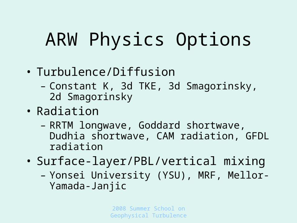
ARW Physics Options
• Turbulence/Diffusion– Constant K, 3d TKE, 3d Smagorinsky, 2d
Smagorinsky
• Radiation– RRTM longwave, Goddard shortwave, Dudhia
shortwave, CAM radiation, GFDL radiation
• Surface-layer/PBL/vertical mixing– Yonsei University (YSU), MRF, Mellor-Yamada-
Janjic

2008 Summer School on Geophysical Turbulence
ARW Physics Options
• Land Surface– Noah, RUC, 5-layer thermal soil– Water can be updated only through reading SST
during run
• Cumulus Parameterization– Kain-Fritsch, Betts-Miller-Janjic, Grell-Devenyi
ensemble
• Microphysics– Kessler, Lin et al., Ferrier, Thompson et al., WSM
(Hong, Dudhia and Chen) schemes
2008 Summer School on Geophysical Turbulence
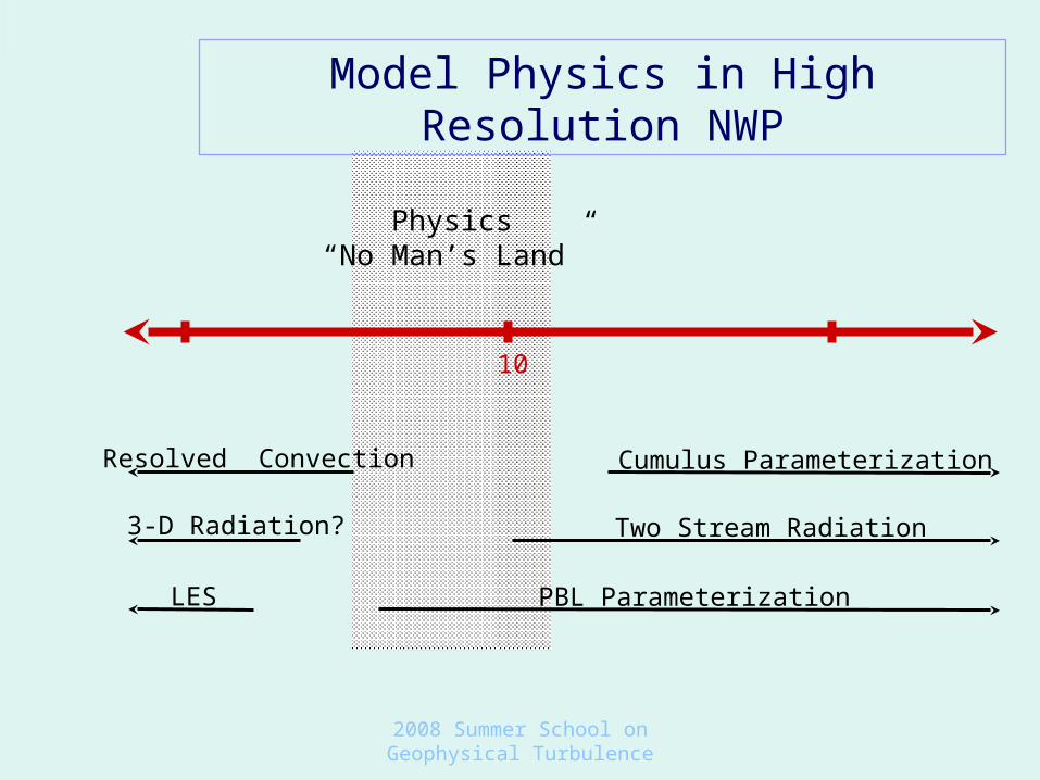
1 10 100 km
Cumulus ParameterizationResolved Convection
LES PBL Parameterization
Two Stream Radiation3-D Radiation?
Model Physics in High Resolution NWP
Physics“No Man’s Land”
2008 Summer School on Geophysical Turbulence
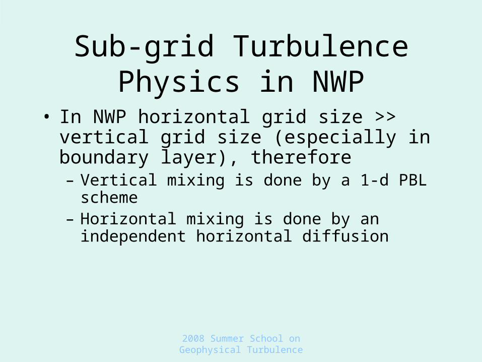
Sub-grid Turbulence Physics in NWP
• In NWP horizontal grid size >> vertical grid size (especially in boundary layer), therefore– Vertical mixing is done by a 1-d PBL scheme– Horizontal mixing is done by an independent
horizontal diffusion

2008 Summer School on Geophysical Turbulence
Role of PBL schemes in NWP
• PBL scheme receives surface fluxes of heat and moisture from land-surface model, and surface stress from surface-layer scheme
• Mixes heat, moisture and momentum in the atmospheric column providing rates of change for these quantities back to the NWP model
• Includes vertical diffusion in free atmosphere• Schemes are mostly distinguished by various
treatments of the unstable boundary layer• Two popular schemes in WRF: YSU and MYJ

2008 Summer School on Geophysical Turbulence
2008 Summer School on Geophysical Turbulence
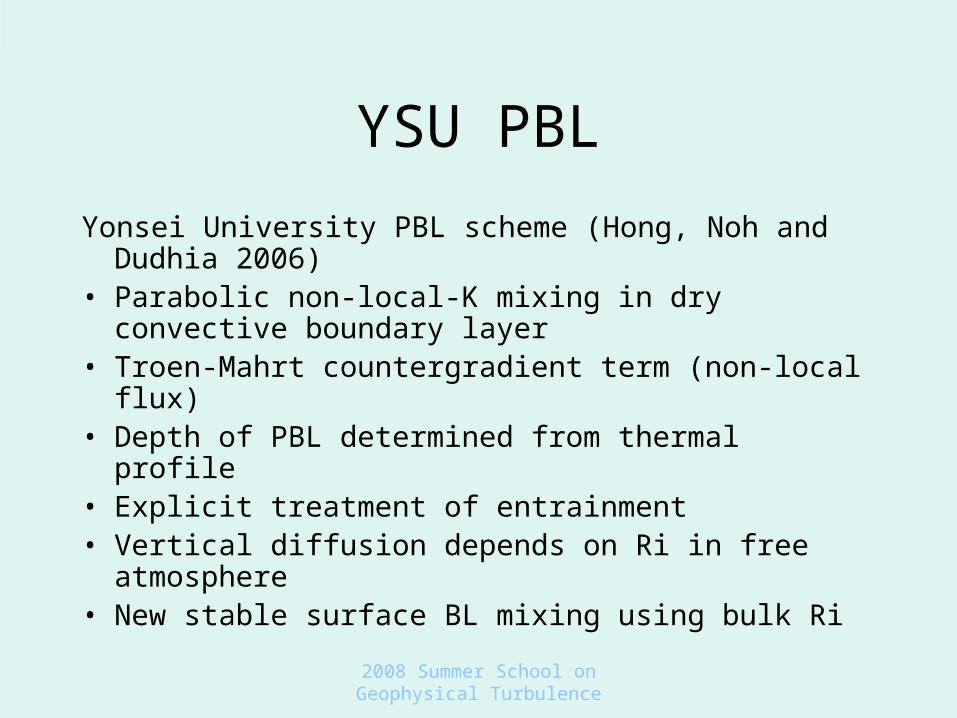
YSU PBL
Yonsei University PBL scheme (Hong, Noh and Dudhia 2006)
• Parabolic non-local-K mixing in dry convective boundary layer
• Troen-Mahrt countergradient term (non-local flux)• Depth of PBL determined from thermal profile• Explicit treatment of entrainment• Vertical diffusion depends on Ri in free atmosphere• New stable surface BL mixing using bulk Ri
2008 Summer School on Geophysical Turbulence
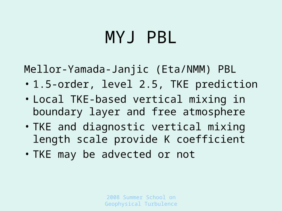
MYJ PBL
Mellor-Yamada-Janjic (Eta/NMM) PBL
• 1.5-order, level 2.5, TKE prediction
• Local TKE-based vertical mixing in boundary layer and free atmosphere
• TKE and diagnostic vertical mixing length scale provide K coefficient
• TKE may be advected or not
2008 Summer School on Geophysical Turbulence
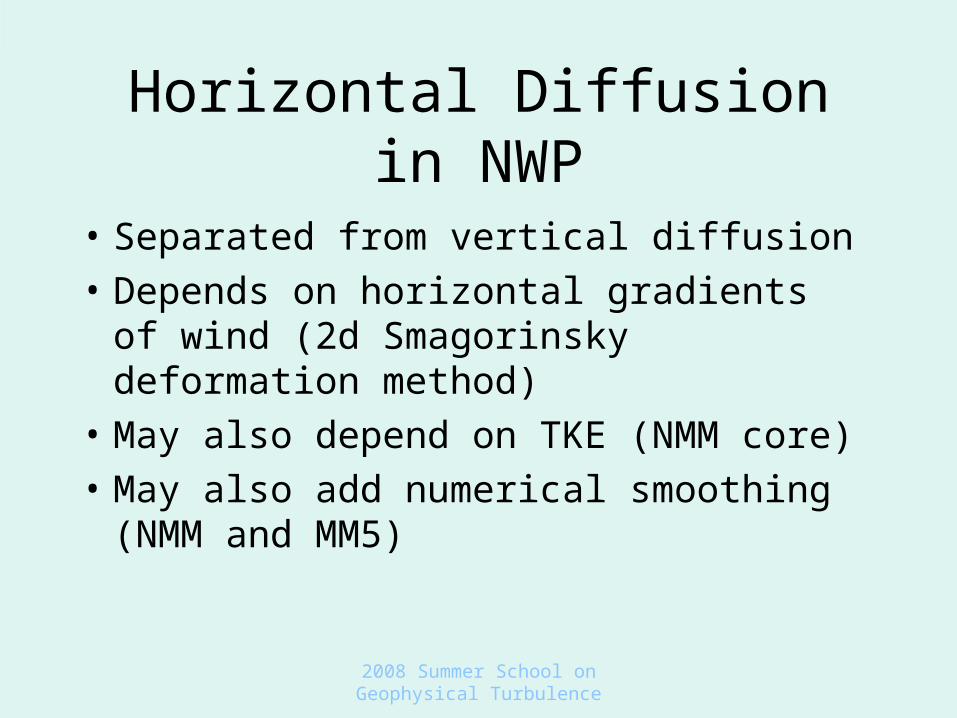
Horizontal Diffusion in NWP
• Separated from vertical diffusion
• Depends on horizontal gradients of wind (2d Smagorinsky deformation method)
• May also depend on TKE (NMM core)
• May also add numerical smoothing (NMM and MM5)
2008 Summer School on Geophysical Turbulence
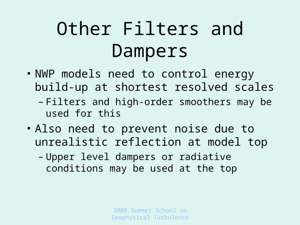
Other Filters and Dampers
• NWP models need to control energy build-up at shortest resolved scales– Filters and high-order smoothers may be
used for this
• Also need to prevent noise due to unrealistic reflection at model top– Upper level dampers or radiative
conditions may be used at the top

2008 Summer School on Geophysical Turbulence
Applications of Regional Models
• Regional Climate
• NWP
2008 Summer School on Geophysical Turbulence
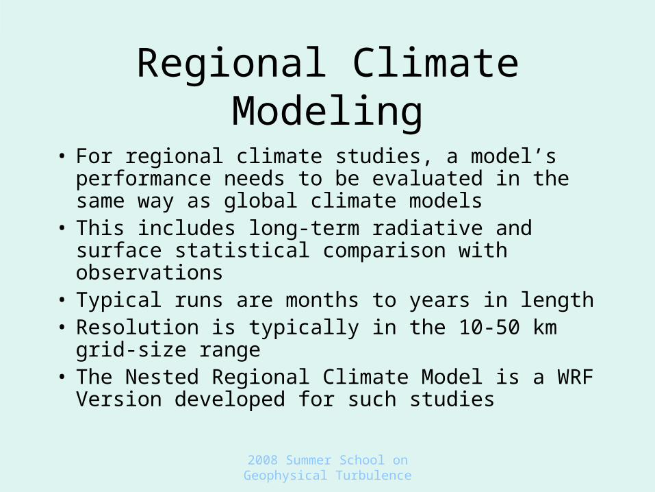
Regional Climate Modeling
• For regional climate studies, a model’s performance needs to be evaluated in the same way as global climate models
• This includes long-term radiative and surface statistical comparison with observations
• Typical runs are months to years in length• Resolution is typically in the 10-50 km grid-
size range• The Nested Regional Climate Model is a
WRF Version developed for such studies
2008 Summer School on Geophysical Turbulence
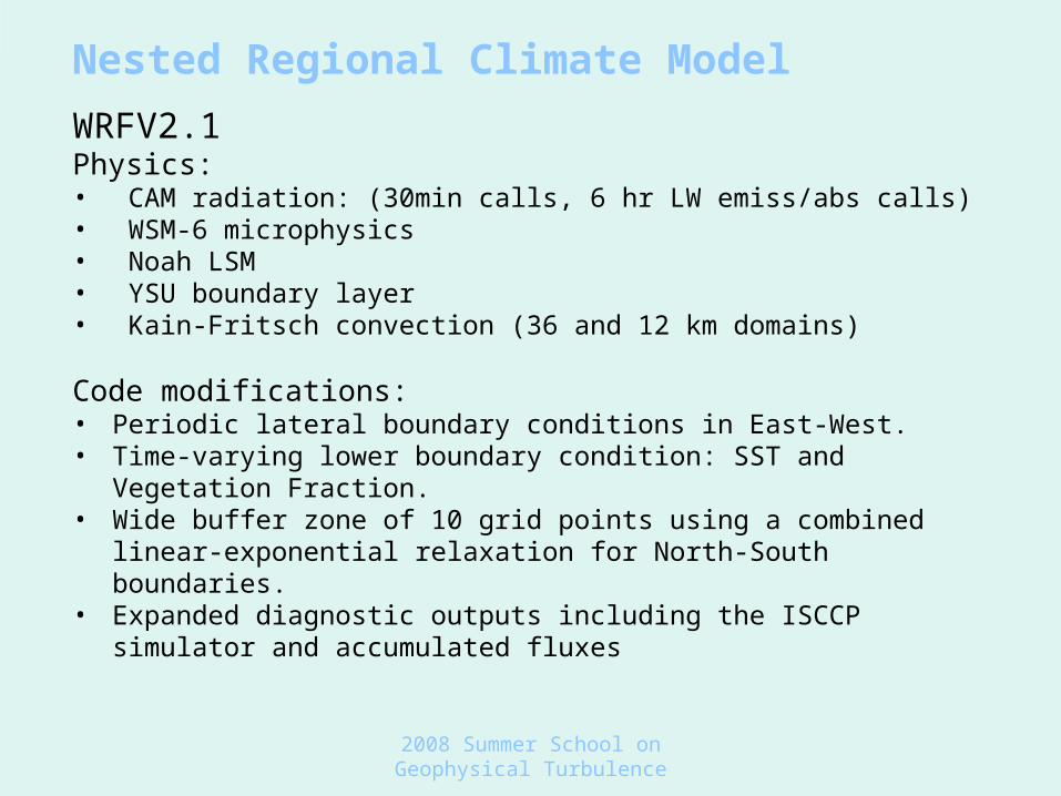
Nested Regional Climate Model
WRFV2.1Physics:• CAM radiation: (30min calls, 6 hr LW emiss/abs calls)• WSM-6 microphysics• Noah LSM• YSU boundary layer• Kain-Fritsch convection (36 and 12 km domains)
Code modifications:• Periodic lateral boundary conditions in East-West.• Time-varying lower boundary condition: SST and Vegetation Fraction.• Wide buffer zone of 10 grid points using a combined linear-exponential relaxation
for North-South boundaries.• Expanded diagnostic outputs including the ISCCP simulator and accumulated
fluxes
2008 Summer School on Geophysical Turbulence
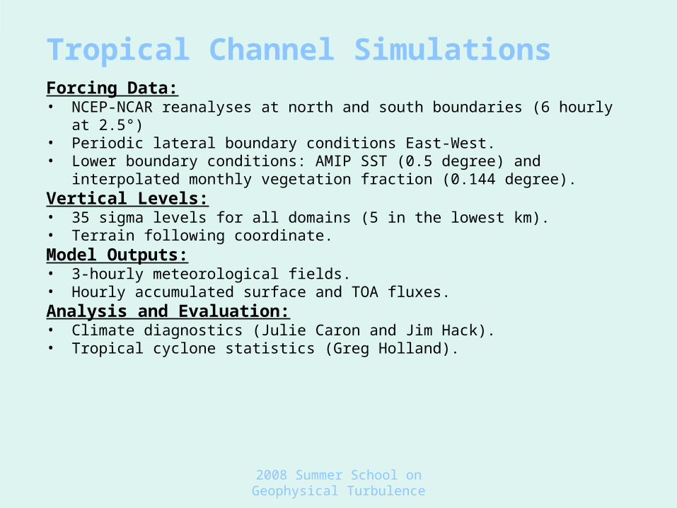
Tropical Channel SimulationsForcing Data:• NCEP-NCAR reanalyses at north and south boundaries (6 hourly at 2.5°)• Periodic lateral boundary conditions East-West.• Lower boundary conditions: AMIP SST (0.5 degree) and interpolated monthly vegetation
fraction (0.144 degree).Vertical Levels:• 35 sigma levels for all domains (5 in the lowest km).• Terrain following coordinate.Model Outputs:• 3-hourly meteorological fields.• Hourly accumulated surface and TOA fluxes.Analysis and Evaluation:• Climate diagnostics (Julie Caron and Jim Hack).• Tropical cyclone statistics (Greg Holland).
2008 Summer School on Geophysical Turbulence
Outgoing Longwave Radiation
QuickTime™ and aBMP decompressor
are needed to see this picture.

2008 Summer School on Geophysical Turbulence
Regional Climate Applications
• Regional climate models may be driven by global climate models for future scenarios (downscaling)
• Emphasis on surface temperature and moisture means turbulence in the boundary layer is central to predictions
• Use of models for wind climate mapping (wind energy applications)
• Regional climate models also used for hydrology studies (water resource applications)
2008 Summer School on Geophysical Turbulence
Air Quality Applications
• Long-term regional model outputs provide input to air-quality/chemistry models
• Input consists of winds and vertical mixing coefficients
• Vertical mixing is important for correct prediction of tracer concentrations near the surface (day-time and nocturnal mixing)

2008 Summer School on Geophysical Turbulence
Numerical Weather Prediction
• Regional NWP models typically are run for a few days
• Boundary conditions come from other models• For real-time forecasts, boundary conditions
come from earlier larger-domain forecasts or ultimately global forecasts (which don’t require boundary conditions) run at operational centers (NCEP global forecast data is freely available in real time on the Web)

2008 Summer School on Geophysical Turbulence
Numerical Weather Prediction
• Time-to-solution is a critical factor in real-time forecasts
• Typically forecasts may be run up to 4 times per day, so each forecast should take only a couple of hours of wall-clock time
• Depending on the region to be covered, computing power constrains the grid size
• For a given region, cost goes as inverse cube of grid length (assuming no change in vertical levels) because time step is approximately proportional to grid length
2008 Summer School on Geophysical Turbulence
Numerical Weather Prediction
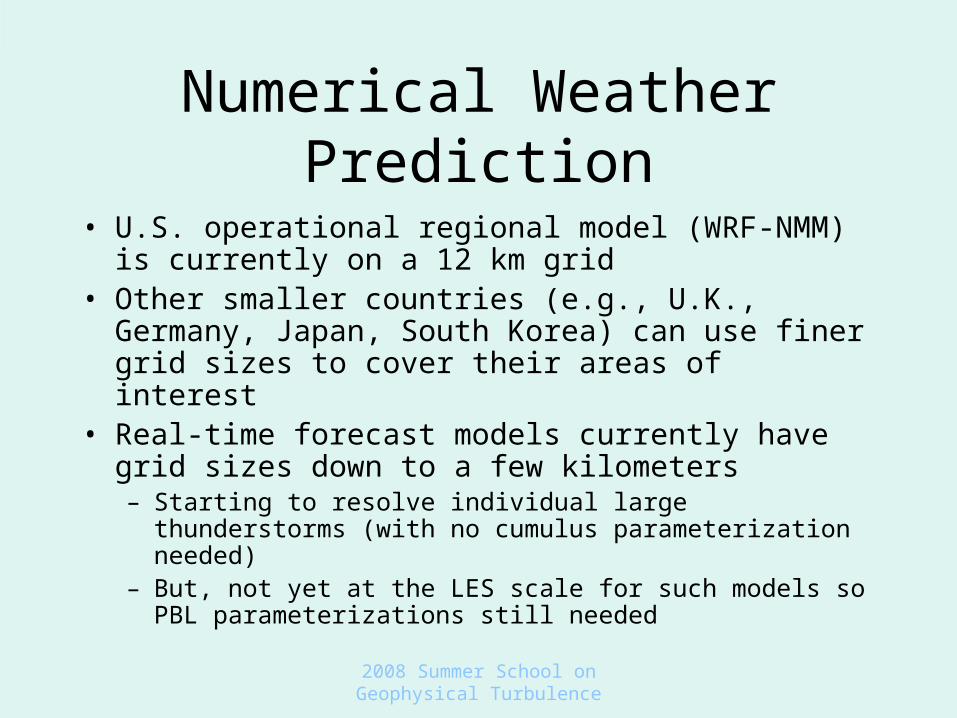
• U.S. operational regional model (WRF-NMM) is currently on a 12 km grid
• Other smaller countries (e.g., U.K., Germany, Japan, South Korea) can use finer grid sizes to cover their areas of interest
• Real-time forecast models currently have grid sizes down to a few kilometers– Starting to resolve individual large thunderstorms (with no
cumulus parameterization needed)– But, not yet at the LES scale for such models so PBL
parameterizations still needed

2008 Summer School on Geophysical Turbulence
Numerical Weather Prediction
• Deterministic versus Ensemble forecasts– Is it better to use given computing resources for
• One high-resolution (deterministic) run, or• Multiple lower-resolution runs (ensemble)
– Now reaching scales where resolution improvements do not necessarily improve forecasts
• Added detail (e.g in rainfall) is not necessarily correctly located• Verification of detailed rainfall forecasts is a key problem
– However, uncertainties in initial conditions are known to exist and to impact forecasts
– Ensembles give an opportunity to explore the range of uncertainty in forecasts, can be used in data assimilation, and can provide probabilistic results
2008 Summer School on Geophysical Turbulence
Real-time Forecasting at NCAR
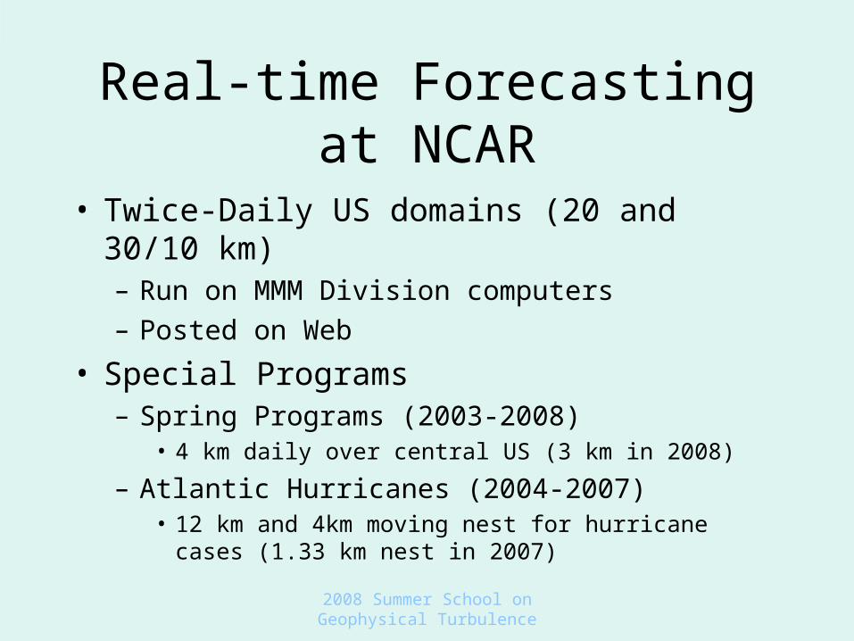
• Twice-Daily US domains (20 and 30/10 km)– Run on MMM Division computers– Posted on Web
• Special Programs– Spring Programs (2003-2008)
• 4 km daily over central US (3 km in 2008)
– Atlantic Hurricanes (2004-2007)• 12 km and 4km moving nest for hurricane cases (1.33
km nest in 2007)
2008 Summer School on Geophysical Turbulence
Spring Programs
• Purpose is to evaluate benefits of convection-resolving real-time simulations to forecasters in an operational situation
• Single hi-res domain run daily from 00z for 36 hours to gauge next day’s convective potential
• Sometimes (as with BAMEX 2003) done in conjunction with field program
2008 Summer School on Geophysical Turbulence
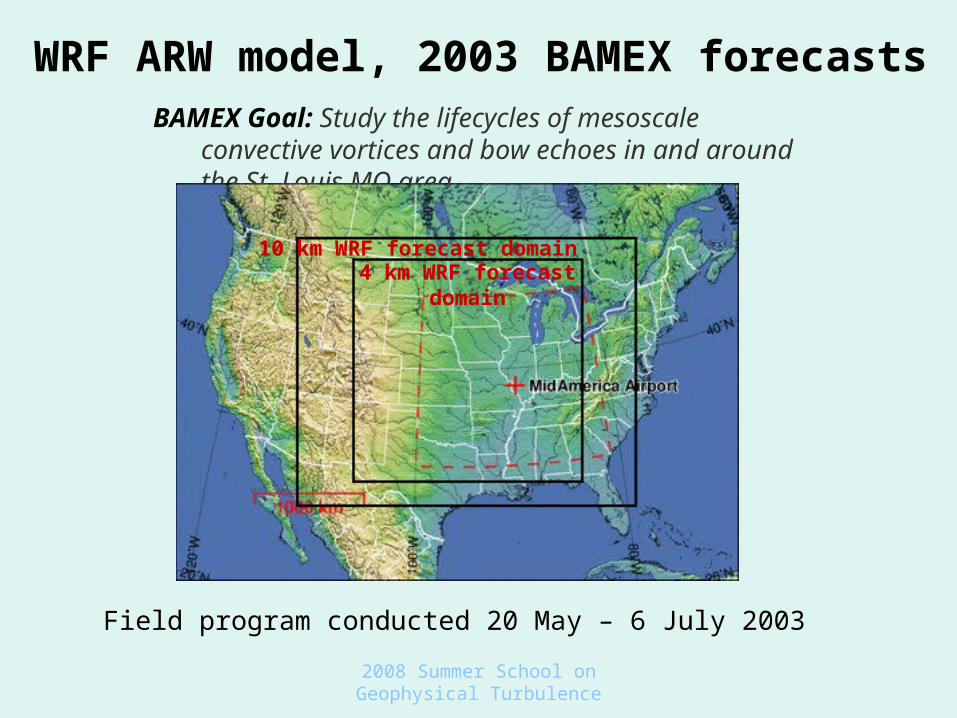
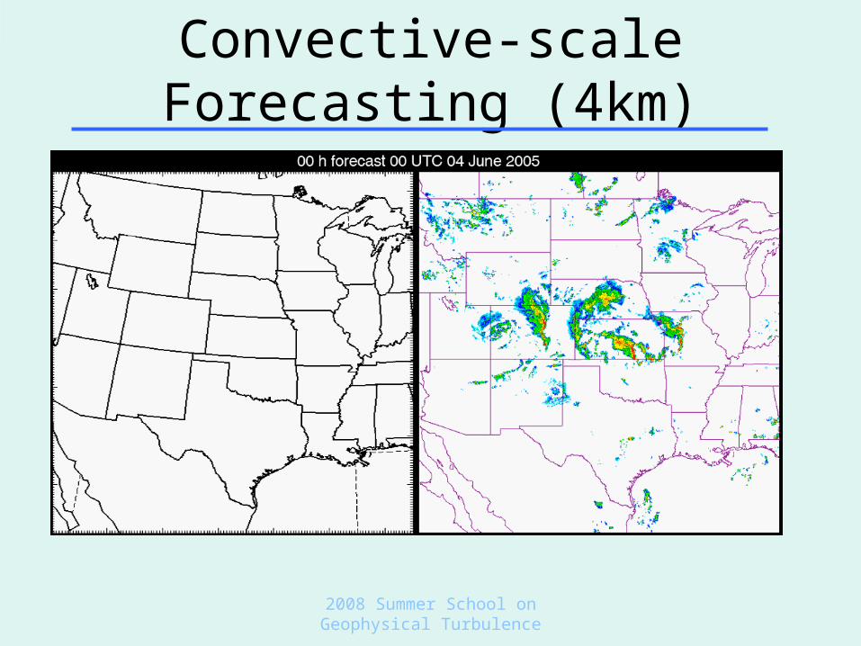
WRF ARW model, 2003 BAMEX forecastsBAMEX Goal: Study the lifecycles of mesoscale convective vortices
and bow echoes in and around the St. Louis MO area
10 km WRF forecast domain4 km WRF forecast domain
Field program conducted 20 May – 6 July 2003
2008 Summer School on Geophysical Turbulence
Convective-scale Forecasting (4km)

2008 Summer School on Geophysical Turbulence
Spring Program Results
• First-generation convection often is well forecast up to 24 hours
• Sometimes next generation is missed or over-forecast
• Forecasters find these products useful
• Give a good idea of convective mode (supercells vs squall lines)

2008 Summer School on Geophysical Turbulence
Study of Resolved Turbulence in NWP
• WRF Kinetic energy spectra study by Skamarock (2005)– How well does the model reproduce observed
spectrum?– How does spectrum change with model
resolution?– How does spectrum vary with meteorological
situation?– How does spectrum develop in model?– How do different models do?

2008 Summer School on Geophysical Turbulence
Kinetic Energy Spectra
Nastrom and Gage (1985)Spectra computed from GASP observations(commercial aircraft)
Lindborg (1999) functionalfit from MOZAIC observations (aircraft)
2008 Summer School on Geophysical Turbulence
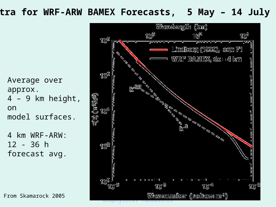
Spectra for WRF-ARW BAMEX Forecasts, 5 May – 14 July 2003
Average over approx.4 – 9 km height, on model surfaces.
4 km WRF-ARW:12 - 36 h forecast avg.
From Skamarock 2005

2008 Summer School on Geophysical Turbulence
Spectra for WRF-ARW BAMEX Forecasts, 1 June – 3 June 2003
Average over approx.4 – 9 km height, on model surfaces.
4, 10 and 22 km WRF-ARW:12 - 36 h forecast avg.
From Skamarock 2005
2008 Summer School on Geophysical Turbulence
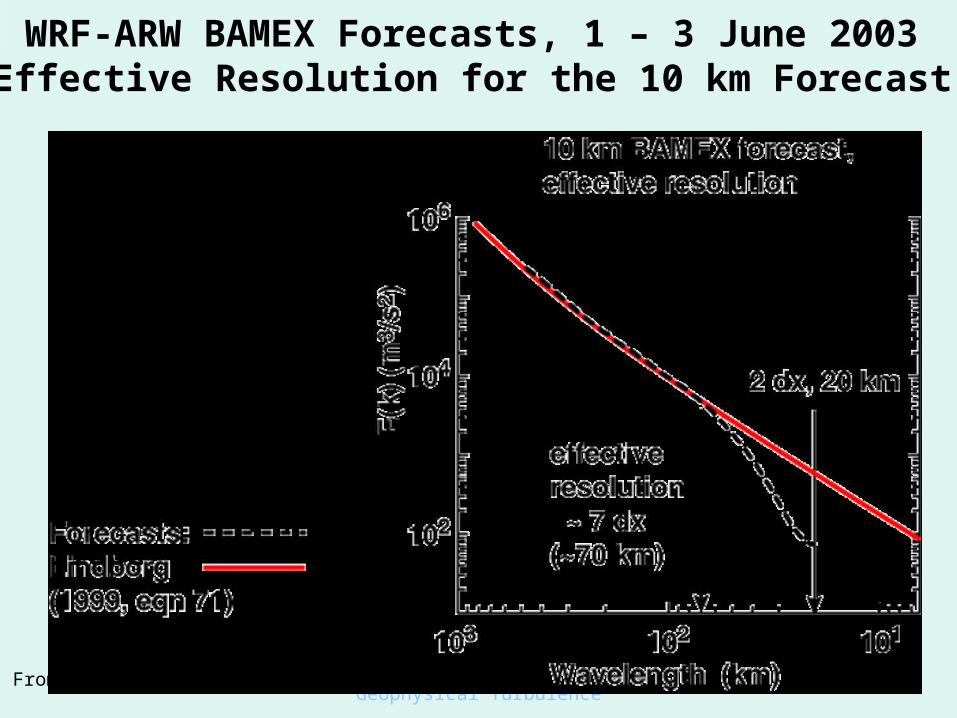
WRF-ARW BAMEX Forecasts, 1 – 3 June 2003Effective Resolution for the 10 km Forecast
Resolution limit determined by locating where Forecast E(k) slope drops below theexpected E(k) slope
From Skamarock 2005

2008 Summer School on Geophysical Turbulence
WRF-ARW BAMEX Forecasts, 1 – 3 June 2003,Effective Resolutions for 22 and 4 km Forecasts
From Skamarock 2005

2008 Summer School on Geophysical Turbulence
Spectra for WRF-ARW Forecasts, Ocean and Continental Cases
Average over approx.4 – 9 km height, on model surfaces.
10 km WRF-ARW:12 - 36 h forecast avg.
From Skamarock 2005
2008 Summer School on Geophysical Turbulence
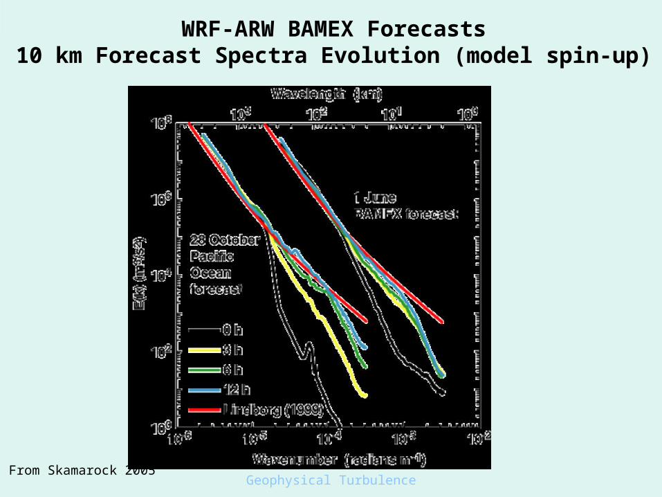
WRF-ARW BAMEX Forecasts10 km Forecast Spectra Evolution (model spin-up)
From Skamarock 2005
2008 Summer School on Geophysical Turbulence
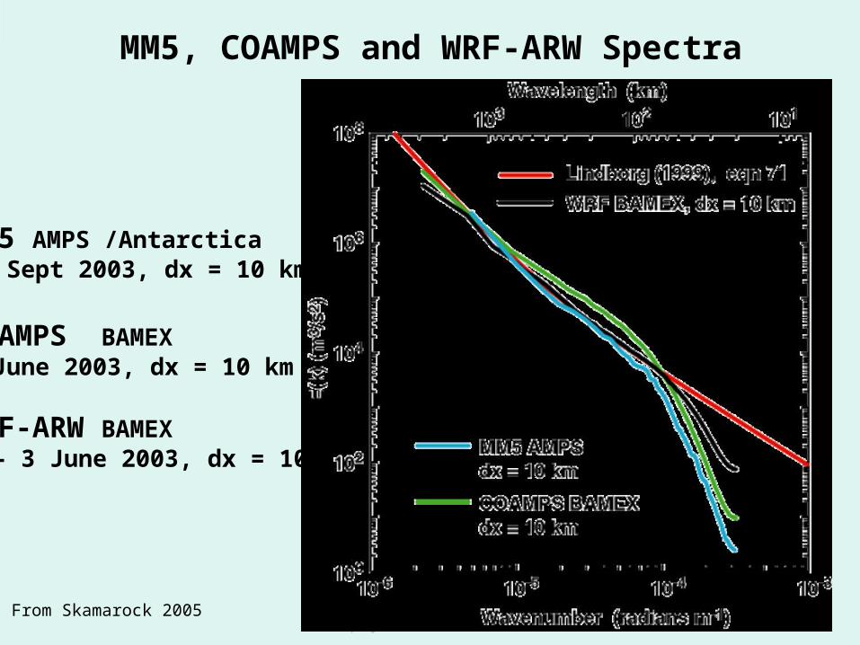
MM5 AMPS /Antarctica 20 Sept 2003, dx = 10 km
COAMPS BAMEX 2 June 2003, dx = 10 km
WRF-ARW BAMEX 1 – 3 June 2003, dx = 10 km
MM5, COAMPS and WRF-ARW Spectra
From Skamarock 2005
2008 Summer School on Geophysical Turbulence
Spectra Results
• ARW captures -3 to -5/3 transition at scales of a few hundred km
• ARW model spectrum resolution is effectively 7 grid lengths (damped below that)
• Different models have different effective resolutions for a given grid size
• Finer scales take ~6 hours to fully develop from coarse analyses
2008 Summer School on Geophysical Turbulence
Hurricane Season Forecasts
• All hurricane cases have been run in real-time with a 4 km moving nest since 2004
• This includes the four Florida storms in 2004 and the major storms Katrina, Rita and Wilma in 2005

2008 Summer School on Geophysical Turbulence
Hurricane Katrina Simulation (4km)
2008 Summer School on Geophysical Turbulence
Hurricane Forecast Tests
• Statistical evaluation against operational models in 2005 showed WRF had better skill in track and intensity beyond 3 days (similar skill before that) (study by Mark DeMaria)
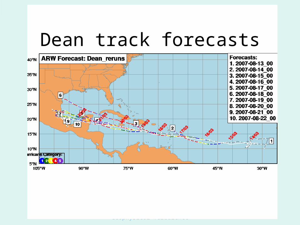
• Many re-runs have shown sensitivities to surface flux treatment (Cd and Ck), and grid size (example is Hurricane Dean of 2007)
• Also investigating 1d ocean-mixed layer feedback
2008 Summer School on Geophysical Turbulence
Dean track forecasts

2008 Summer School on Geophysical Turbulence
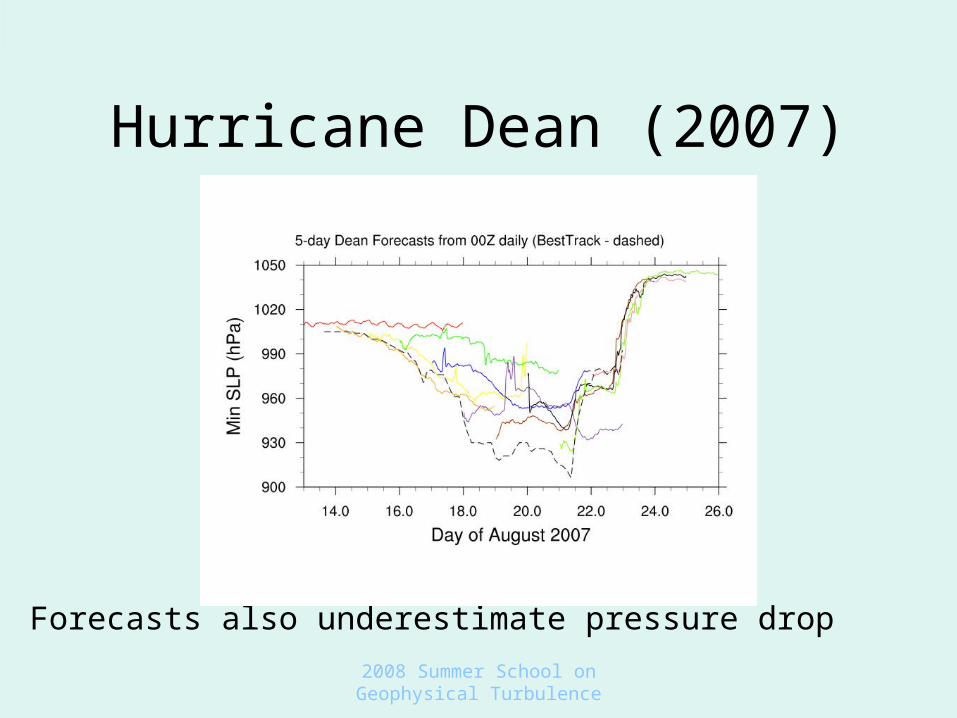
Hurricane Dean (2007)
Note that forecasts underestimate maximum windspeed
2008 Summer School on Geophysical Turbulence
Hurricane Dean (2007)
Forecasts also underestimate pressure drop
2008 Summer School on Geophysical Turbulence
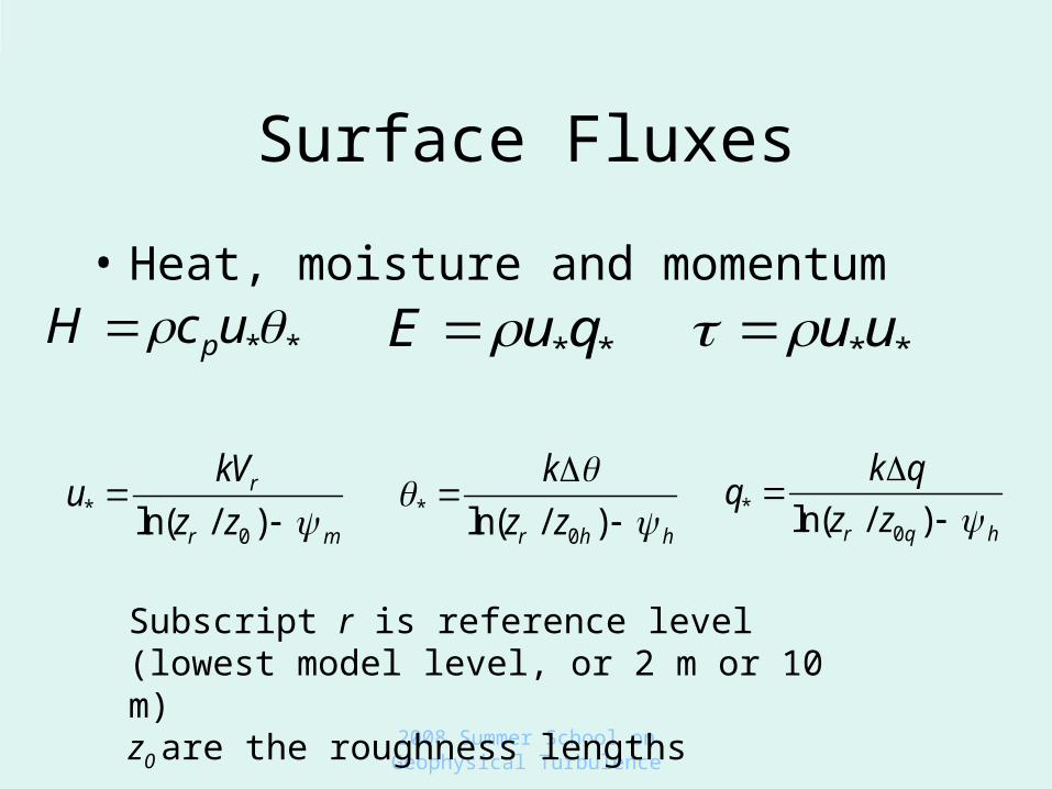
Surface Fluxes
• Heat, moisture and momentumH cpu** u*u*E u*q*
u* kVr
ln(zr / z0 ) m
* k
ln(zr / z0h ) h
q* kq
ln(zr / z0q ) h
Subscript r is reference level (lowest model level, or 2 m or 10 m)z0 are the roughness lengths

2008 Summer School on Geophysical Turbulence
Roughness Lengths
• Roughness lengths are a measure of the “initial” length scale of surface eddies, and generally differ for velocity and scalars
• In 2006 AHW z0h=z0q are calculated based on Carlson-Boland (~10-4 m for water surfaces, weak variation with wind speed)
• z0 for momentum is a function of wind speed following tank experiments of Donelan (this replaces the Charnock relation in WRF). This represents the effect of wave heights in a simple way.

2008 Summer School on Geophysical Turbulence
Drag Coefficient
• CD10 is the 10 m drag coefficient, defined such that
CD10 k
ln(z10 / z0 )
2
It is related to the roughness length by (in neutral conditions)
CD10V102
2008 Summer School on Geophysical Turbulence
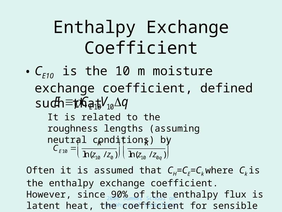
Enthalpy Exchange Coefficient
• CE10 is the 10 m moisture exchange coefficient, defined such that
CE10 k
ln(z10 / z0 )
k
ln(z10 / z0q )
It is related to the roughness lengths (assuming neutral conditions) by
Often it is assumed that CH=CE=Ck where Ck is the enthalpy exchange coefficient. However, since 90% of the enthalpy flux is latent heat, the coefficient for sensible heat (CH) matters less than that for moisture (CE)
E CE10V10q

2008 Summer School on Geophysical Turbulence
CD and Ck
• From the works of Emanuel (1986), Braun and Tao (2001) and others the ratio of Ck to CD is an important factor in hurricane intensity
• Observations give some idea of how these coefficients vary with wind speed but generally have not been made for hurricane intensity

2008 Summer School on Geophysical Turbulence
Black et al. (2006)
27th AMS Hurricane conference
2008 Summer School on Geophysical Turbulence
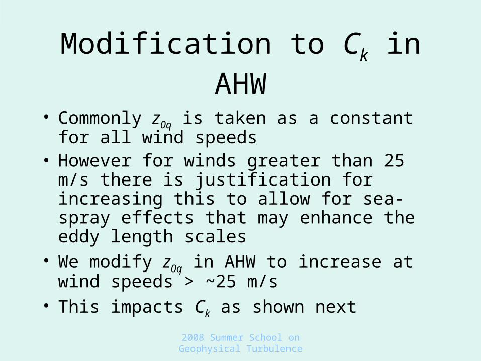
Modification to Ck in AHW
• Commonly z0q is taken as a constant for all wind speeds
• However for winds greater than 25 m/s there is justification for increasing this to allow for sea-spray effects that may enhance the eddy length scales
• We modify z0q in AHW to increase at wind speeds > ~25 m/s
• This impacts Ck as shown next

2008 Summer School on Geophysical Turbulence
Modification to Ck in AHW
Cd - redOld CB - greenNew Ck - blue
dashedZ0q const - blue
solid

2008 Summer School on Geophysical Turbulence

2008 Summer School on Geophysical Turbulence

2008 Summer School on Geophysical Turbulence
QuickTime™ and aBMP decompressor
are needed to see this picture.

2008 Summer School on Geophysical Turbulence
Hurricane Physics
• Results here and elsewhere demonstrate sensitivity of simulated intensity to surface flux formulation
• Also need to add dissipative heating from friction (Bister and Emanuel)
• Other aspects of physics also affect hurricane structure (e.g. microphysics)

2008 Summer School on Geophysical Turbulence
Towards LES Modeling
• LES scales (~100 m grids or less)• NWP not yet at LES scales, but maybe
in a decade or two it will be• Need to evaluate how LES does for
challenging situations like hurricanes• Study by Yongsheng Chen et al. is an
example of an early attempt using an idealized hurricane

2008 Summer School on Geophysical Turbulence
Large Eddy Simulations of an Idealized Hurricane
Yongsheng Chen, Rich Rotunno, Wei Wang, Christopher Davis, Jimy Dudhia, Greg Holland
MMM/NCAR
37km
Motivation
1. Intensity sensitivity to model resolution
2. Direct computation of effects of turbulence
2008 Summer School on Geophysical Turbulence
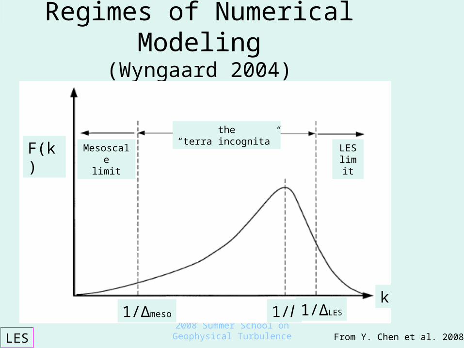
Regimes of Numerical Modeling(Wyngaard 2004)
LES
1/Δmeso 1/ΔLES1/l
Mesoscale
limit
LESlimit
the“terra incognita”
k
F(k)
From Y. Chen et al. 2008

2008 Summer School on Geophysical Turbulence
Model Setup
LES
Idealized TCf-plane zero env windfixed SST
Nested Grids
WRF Model PhysicsWSM3 simple iceNo radiationRelax to initial temp.Cd (Donelan)Ck (Carlson-Boland)Ck/Cd ~ 0.65YSU PBLLES PBL
( 1.67km)( 1.67km)
6075km
1500km1000km
333km111km
37km
( 15km)
( 5km)( 1.67km)
( 556m)( 185m)
( 62m)
50 vertical levelsz=60m~1kmZtop=27km
From Y. Chen et al. 2008
2008 Summer School on Geophysical Turbulence
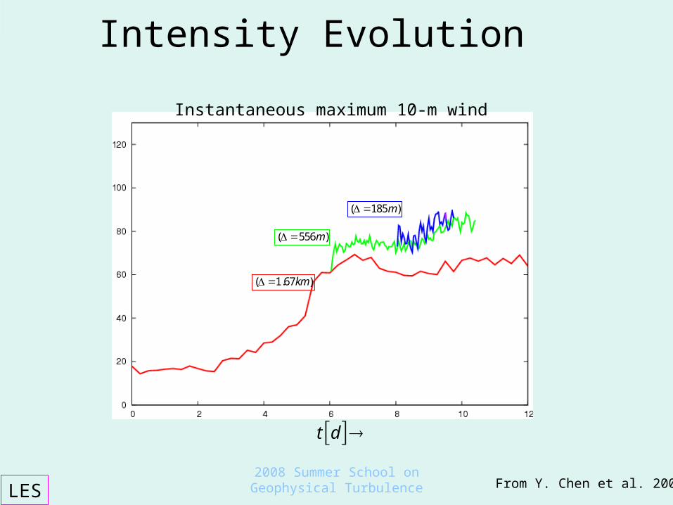
Intensity Evolution
LES
t d
( 1.67km)
( 556m)
( 185m)
( 62m)
Instantaneous maximum 10-m wind
From Y. Chen et al. 2008
2008 Summer School on Geophysical Turbulence
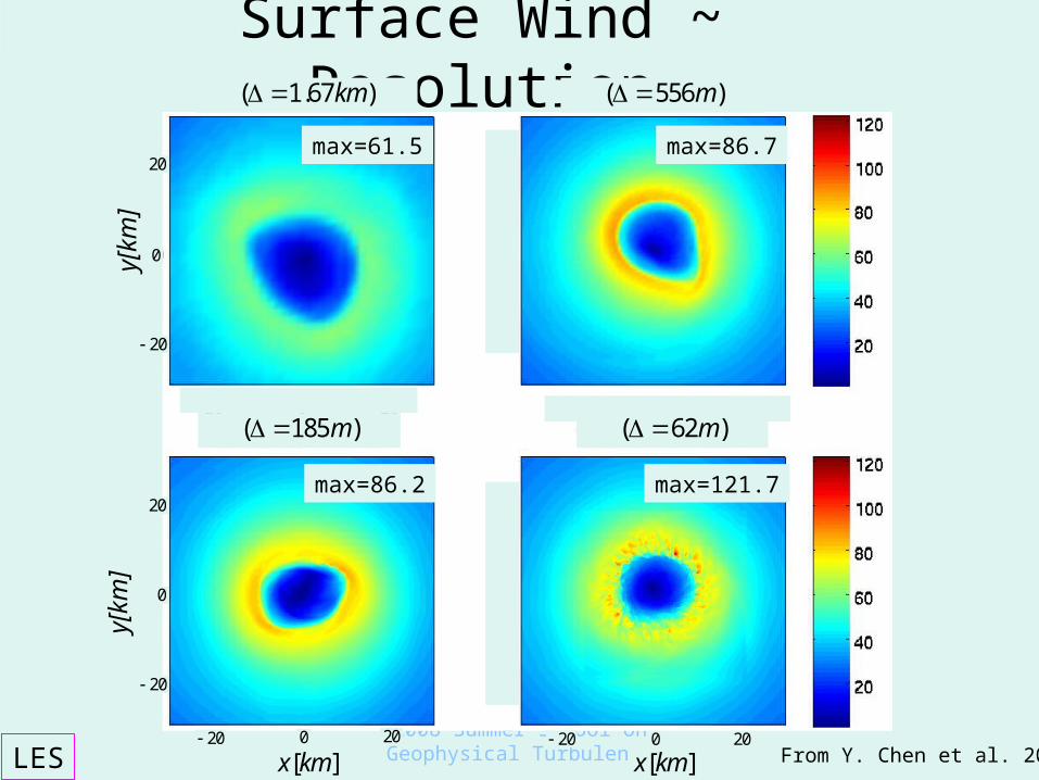
Surface Wind ~ Resolution
LES
( 1.67km) ( 556m)
( 185m)
2020
20
20
20 20
20
20
00
0
0
x[km] x[km]
y[km]
y[km]
( 62m)
max=61.5
max=121.7max=86.2
max=86.7
From Y. Chen et al. 2008

2008 Summer School on Geophysical Turbulence
1-min Averaged Surface Wind
LES
37km 37 km
Max=85.5 Max=82.3 Max=83.7
instantaneous 1-min average
max=121.7 max=78.8
From Y. Chen et al. 2008

2008 Summer School on Geophysical Turbulence
Eddy Kinetic Energy Spectra
LES
( 1.67km) ( 556m) ( 185m)( 62m)
From Y. Chen et al. 2008

2008 Summer School on Geophysical Turbulence
LES Hurricane Tests
• At 62 meter grid, eddies become resolved representing individual gusts
• Issues remain– Near ground LES schemes lack proper
treatment of reduced eddy sizes, since much kinetic energy should remain in sub-grid-scale turbulence there
– Therefore, never possible to fully resolve turbulence near surface
2008 Summer School on Geophysical Turbulence
Summary and Conclusions
• Regional modeling and NWP rely on turbulence parameterizations– PBL schemes and vertical diffusion– Horizontal diffusion– Surface eddy transports– (also) Gravity-wave drag
• Forecast skill depends on methods used• Better parameterizations for these processes
are being developed in ongoing research


