Mon. Not. R. Astron. Soc. 000, 000–000 (0000) Printed 23 October 2014 (MN LATEX style file v2.2)
Metallicity gradients in local field star-forming galaxies: Insights on
inflows, outflows, and the coevolution of gas, stars and metals
I-Ting Ho1, Rolf-Peter Kudritzki1,2, Lisa J. Kewley1,3, H. Jabran Zahid4,
Michael A. Dopita3,5, Fabio Bresolin1, and David S. N. Rupke61Institute for Astronomy, University of Hawaii, 2680 Woodlawn Drive, Honolulu, HI 96822, USA2University Observatory Munich, Scheinerstr. 1, D-81679 Munich, Germany3Research School of Astronomy and Astrophysics, Australian National University, Cotter Road, Weston ACT 2611, Australia4Harvard-Smithsonian Center for Astrophysics, 60 Garden Street MS-20, Cambridge, MA 02138, USA5Astronomy Department, King Abdulaziz University, P.O. Box 80203, Jeddah, Saudi Arabia6Department of Physics, Rhodes College, Memphis, TN 38112, USA
Accepted ??. Received ??; in original form ??
ABSTRACT
We present metallicity gradients in 49 local field star-forming galaxies. We derive gas-phase oxygen abundances using emission line ratios with two widely adopted metallicitycalibrations based on the [O III]/Hβ, [N II]/Hα and [N II]/[O II] line ratios. The two derivedmetallicity gradients are usually in good agreement within ±0.14 dexR−1
25(R25 is the B-band
iso-photoal radius of 25th magnitude/arcsec2), but we show that the metallicity gradients candiffer significantly when the ionisation parameters change systematically with radius. We in-vestigate the metallicity gradients as a function of stellar mass (8 < log(M∗/M⊙) < 11)and absolute B-band luminosity (−16 > MB > −22). When the metallicity gradients areexpressed in dex kpc−1, we show that galaxies with lower mass and luminosity, on average,have steeper metallicity gradients. When the metallicity gradients are expressed in dexR−1
25to
take into account their sizes, we find no correlation between the metallicity gradients, and stel-lar mass and luminosity, in agreement with previous studies. We provide a local benchmarkmetallicity gradient of field star-forming galaxies useful for comparison with future studiesat high redshifts. To investigate the origin of the local benchmark gradient, we adopt simplechemical evolution models to constrain the relationship between metallicity and stellar-to-gas mass ratio. The models reproduce the local benchmark gradient using the observed gasand stellar surface density profiles in nearby field spiral galaxies. Our models suggest thatthe local benchmark gradient is a direct result of the coevolution of gas and stellar disk un-der virtually closed-box chemical evolution when the stellar-to-gas mass ratio becomes high(≫ 0.3). These models imply low current mass accretion rates (. 0.3× SFR), and low massoutflow rates (. 2.5× SFR) in local field star-forming galaxies.
Key words:
1 INTRODUCTION
The content of heavy elements in a galaxy is one of the key
properties for understanding its formation and evolutionary his-
tory. The gas-phase oxygen abundance in the interstellar medium
(ISM) of a galaxy (or “metallicities”), defined as the number
ratio of oxygen to hydrogen atom and commonly expressed as
12 + log(O/H), is regulated by various processes during the evo-
lutionary history of a galaxy. While the oxygen is predominately
synthesised in high-mass stars (> 8M⊙) and subsequently released
to the ISM by stellar winds and supernova explosion, the oxygen
in the ISM could also be expelled to the circumgalactic medium,
or potentially become gravitationally unbound, via feedback pro-
cesses, e.g. galactic-scale outflows. Gas inflows triggered by merg-
ers and inflows of pristine gas from the intergalactic medium could
also dilute the metallicity of a galaxy (e.g. Kewley et al. 2006a;
Rupke et al. 2008; Kewley et al. 2010; Rupke et al. 2010a,b). The
relations between metallicity and other fundamental properties of
galaxies can place tight constraints on the processes governing the
evolution of galaxies.
The correlation between global metallicity and stellar mass
in star-forming galaxies, i.e. the mass-metallicity relation, is one
of the fundamental relations for measuring the chemical evolu-
tion of galaxies (Lequeux et al. 1979; Tremonti et al. 2004). Whilst
the mass-metallicity relation was first established locally, mod-
ern spectroscopic surveys have enabled precise measurements of

2 Ho et al.
metallicity out to high redshifts on large numbers of galaxies
(e.g., Savaglio et al. 2005; Erb et al. 2006; Zahid et al. 2011, 2013,
2014b; Wuyts et al. 2014; Steidel et al. 2014; Sanders et al. 2014)
and laid the foundation for subsequent investigation into the phys-
ical origin of the relation. Various physical processes including
metal enriched outflows (e.g., Larson 1974; Tremonti et al. 2004),
accretion of metal-free gas (e.g. Dalcanton et al. 2004), and varia-
tion in the initial mass function (Koppen et al. 2007) or star forma-
tion efficiency (e.g., Brooks et al. 2007; Calura et al. 2009) have all
been proposed to be responsible for shaping the mass-metallicity
relation. The mass-metallicity relation may also have an additional
dependency on star formation rate (SFR; e.g., Mannucci et al.
2010; Lara-Lopez et al. 2010; Yates et al. 2012). Spatially resolved
studies have shown that the mass-metallicity relation also holds
on smaller scales for individual star-forming regions within galax-
ies (Rosales-Ortega et al. 2012). Recent work suggests that the
mass-metallicity relation could be a direct result of some more
fundamental relations between metallicity, stellar and gas content
(Zahid et al. 2014c; Ascasibar et al. 2014).
The spatial distribution of metals in a disk galaxy can also
provide critical insight into its mass assembly history. Disk galax-
ies in the local Universe universally exhibit negative metallic-
ity gradients, i.e., the centre of a galaxy has a higher metallicity
than the outskirts (e.g., Zaritsky et al. 1994; Moustakas et al. 2010;
Rupke et al. 2010b; Sanchez et al. 2014, and references therein). In
several cases, where measurements are possible out to very larger
radii (2×R251), the metallicity gradients flatten in the outer disks,
suggesting inner-to-outer transportation of metals via mechanisms
such as galactic fountains (e.g., Werk et al. 2011; Bresolin et al.
2012; Kudritzki et al. 2014; Sanchez et al. 2014). Extreme exam-
ples of metal mixing occurs in interacting galaxies, where the non
axis-symmetric potential induces radial inflows of gas. Both ob-
servations and simulations confirm that mergers of disk galaxies
present shallower metallicity gradients than isolated disk galaxies
due to effective gas mixing (e.g., Kewley et al. 2010; Rupke et al.
2008, 2010a,b; Torrey et al. 2012; Rich et al. 2012).
Sophisticated modelling of the evolution of metallicity gra-
dients in disk galaxies has shed light on the formation, gas ac-
cretion, and star formation history of the disks. While the details
vary from model to model, typical assumptions of inside-out disk
growth, no radial matter exchange, and closed-box chemical evolu-
tion can successfully reproduce the current gradients in local galax-
ies (e.g., Chiappini et al. 2001; Fu et al. 2009). However, some
models predict that metallicity gradients steepen with time (e.g.,
Chiappini et al. 1997, 2001; see also Mott et al. 2013 who included
radial inflow), while others predict the opposite (e.g., Molla et al.
1997; Prantzos & Boissier 2000; Fu et al. 2009; Pilkington et al.
2012). Testing the model predictions using observations of high
redshift galaxies are challenging (e.g., Yuan et al. 2011; Jones et al.
2010, 2013, and references therein). In addition, systematic effects
from insufficient resolution and/or binning of the data unfortunately
can seriously the reliability of metallicity gradients measured at
high redshifts (Yuan et al. 2013; Mast et al. 2014).
Statistical studies of metallicity gradients in the local Uni-
verse provide an alternative approach to constrain the theoreti-
cal simulations. Although the measurements are time-consuming,
sample sizes of few tens of galaxies have been achieved in the
past using long-slit spectroscopy. These samples gave intriguing
(and sometimes contradictory) correlations between metallicity
1 Radius of the 25th magnitude/arcsec2 isophote in B-band.
gradients and physical properties of the disk galaxies. For exam-
ple, barred galaxies tend to exhibit shallower metallicity gradi-
ents than non-barred galaxies even when galaxy sizes are taken
into account (e.g., Vila-Costas & Edmunds 1992; Zaritsky et al.
1994), but such discrepancy is insignificant in some recent studies
(Sanchez et al. 2014). For unbarred galaxies, galaxies with higher
B-band luminosity or higher total mass have shallower metallic-
ity gradients (Vila-Costas & Edmunds 1992; Garnett et al. 1997);
however, such behaviour is not pronounced in some measure-
ments (e.g., van Zee et al. 1998; Prantzos & Boissier 2000). Some
studies find that non-barred galaxies show a statistically signif-
icant correlation between metallicity gradient and Hubble Type,
where earlier types have shallower metallicity gradients than later
types (Vila-Costas & Edmunds 1992; Oey & Kennicutt 1993), but
considerable scatter exists in other measurements (Zaritsky et al.
1994). Most studies find no correlation when metallicity gradients
are normalised to some scale-length (i.e.,R25, the disk scale-length
Rd, or the effective radius Re2). The contradictory results of some
earlier studies might be due to the small sample sizes and incon-
sistent methodologies of measuring metallicity gradients. Applying
different metallicity diagnostics can introduce considerable system-
atic errors (Kewley & Ellison 2008).
Advances in instrumentation such as multi-slit spectroscopy
and wide-field integral field spectroscopy (IFS) is in the pro-
cess of revolutionising statistical studies of metallicity gradients
in the local Universe (e.g., Sanchez et al. 2014). Large on-going
and future large IFS surveys include the Calar Alto Legacy In-
tegral Field Area Survey (CALIFA; Sanchez et al. 2012a), the
Sydney-AAO Multi-object Integral field spectrograph (SAMI) Sur-
vey (Croom et al. 2012; Bryant et al. 2014; Allen et al. 2014), the
Mapping Nearby Galaxies at Apache Point Observatory (MaNGA)
Survey, the Hector Survey (Lawrence et al. 2012; Bland-Hawthorn
2014), and many others. These IFS surveys are not only extremely
efficient in collecting large numbers of spectra simultaneously and
seamlessly across an entire galaxy, but also have desirable wave-
length coverage to capture multiple key emission lines for deriving
metallicity. Such features pose a unique opportunity to eliminate
systematic errors using statistical approaches.
In this paper, we study the metallicity gradients in a sample of
49 local field star-forming galaxies. We derive metallicity gradients
using different abundance calibrations and discuss potential sys-
tematic effects induced by the calibrations adopted. We investigate
whether metallicity gradients in field star-forming galaxies corre-
late with their physical properties. We show that there is a common
metallicity gradient in local field star-forming galaxies and we pro-
vide some benchmark values. Finally, we adopt simple chemical
evolution models to explain the formation of the common metallic-
ity gradient.
The paper is structured as follows. We describe our samples,
observations and data reduction in Section 2, and our data analysis
in Section 3. In Section 4, we detail our methodology of deriving
the metallicity, ionisation parameter, and metallicity gradients. In
Section 5, we present our measurements of metallicity gradients,
discuss the systematic effects, and compare the metallicity gradi-
ents with stellar masses and absolute B-band magnitudes. We pro-
vide a benchmark metallicity gradient in Section 6 and investigate
the origin of the benchmark gradient in Section 7 using the sim-
2 The effective radius is the radius at which the integrated flux is half of the
total one. Comparing to the disk scale-length for the classical exponential
profile, Re = 1.67835Rd .
Metallicity gradients in local field star-forming galaxies 3
ple chemical evolution models derived in Appendix A. Finally, a
summary and conclusions are given in Section 8. Through out this
paper, we assume the standard Λ cold dark matter cosmology with
H0 = 70 km s−1 Mpc−1, ΩM = 0.3 and ΩΛ = 0.7.
2 SAMPLES
The 49 galaxies studied in this work are drawn from various
sources, including literature data, public data and our targeted ob-
servations. We describe the four samples in the next four subsec-
tions. The focus of this paper is to investigate field star-forming
galaxies, and therefore we select only field galaxies that are not un-
dergoing major mergers and not in close pairs; none of our galaxies
have massive companions (i.e. stellar mass higher than one-third of
the main galaxies) within 70 kpc in projection and 1000 km s−1 in
line-of-sight velocity separation.
2.1 CALIFA galaxies in Data Release 1
We use the publicly available IFS data from the first data re-
lease (DR1) of the CALIFA survey. A full description of the sur-
vey design, including details of target selection and data reduction
scheme, can be found in Sanchez et al. (2012a). Specific details re-
lated to the DR1 can be found in Husemann et al. (2013, see also
Walcher et al. 2014). Below we briefly summarise the information
relevant to this work.
The CALIFA DR1 contains reduced IFS data of 100 local
galaxies (0.005 < z < 0.03) covered by the Sloan Digital Sky Sur-
vey (SDSS; York et al. 2000; Abazajian et al. 2009). In this study,
we focus only on spiral galaxies that are not undergoing a major
merger, and not in close pairs. Extremely edge-on systems with in-
clination angle larger than 70 are excluded from our analysis since
de-projecting radial distance is uncertain. Systems without enough
sufficiently high signal-to-noise spaxels (S/N > 3) to measure
emission line fluxes are also excluded. In total, 21 CALIFA galax-
ies are analysed.
The released CALIFA datacubes, as processed by the CAL-
IFA automatic data reduction pipeline, have a spatial size of ∼74′′ × 64′′ on a rectangular 1′′ grid. The point spread func-
tion, as measured from field stars in the datacubes, has a me-
dian full-width measured at half-maximum (FWHM) of 3.7′′ . Ev-
ery CALIFA galaxy is observed using the fiber bundle integral
field unit (IFU) PPak, and two different setups with the Pots-
dam Multi-Aperture Spectrophotometer (PMAS; Roth et al. 2005;
Kelz et al. 2006). The low-resolution (V500) and high-resolution
(V1200) setup cover wavelength ranges of ∼ 3745–7500 A and
∼ 3650–4840 A, respectively. The V500 reduced datacubes have a
FWHM spectral resolution of 6.0A (R ∼ 850) and a spectral chan-
nel width of 2.0A. The V1200 reduced datacubes have a FWHM
spectral resolution of 2.3A (R ∼ 1650) and a spectral channel
width of 0.7A.
2.2 WiFeS galaxies
The CALIFA sample was selected based on the angular iso-photal
diameter of the galaxies (45′′ < D25 < 80′′). Therefore, the
CALIFA sample is inevitably biased towards galaxies of higher
mass (& 109 M⊙). To probe metallicity gradients in galaxies of
lower mass in a statistically significant way, we conducted supple-
mental IFS observations to specifically target low mass systems
(i.e., log(M∗/M⊙) = 8–9). We first selected a mother sample
of low-mass galaxies from the SDSS Data Release 7 value added
catalog constructed by the MPA/JHU group3. We used the stellar
mass derived by the MPA/JHU group as a reference for target se-
lection (Kauffmann et al. 2003a; Salim et al. 2007); the final stel-
lar masses adopted in this work are derived separately and con-
sistently for all our samples. As a result of this selection, one of
the WiFeS galaxies presented has a substantially larger final stel-
lar mass (log(M∗/M⊙) ∼ 10.2) due to the incorrect apertures
adopted by MPA/JHU. We remove galaxies with AGN from our
mother sample using the optical line ratios [N II]/Hα and [O III]/Hβ(Kewley et al. 2006b). We further constrained the mother sample
to have low inclination disks and spatial extent comparable to the
Wide Field Spectrograph (see Section 2.2.1). We also visually con-
firmed that these galaxies are not undergoing major merger and do
not have massive companions. From the mother sample, we then
selected our final targets based on observability and instrumental
sensitivity. In total, we observed 19 galaxies, 10 of which yield re-
liable metallicity gradients and are presented in this paper.
2.2.1 Observation and data reduction
We observed our low-mass galaxies using the WiFeS on the 2.3-
m telescope at Siding Spring Observatory in December 2012 and
April 2013. WiFeS is a dual beam, image-slicing IFU consisting
of 25 slitlets. Each slitlet is 38′′ long and 1′′ wide, yielding a
25′′ × 38′′ field of view. For a thorough description of the instru-
ment, see Dopita et al. (2007) and Dopita et al. (2010). Each galaxy
was observed with the blue and red arms simultaneously using
the B3000 and R7000 gratings, respectively. All galaxies were ob-
served with a single WiFeS pointing except for J031752.75-071804
where we adopted a two-point mosaic. The typical exposure time
is ∼ 1− 2 hours per galaxy under seeing conditions of 1.5− 2.5′′ .We reduce the data using the custom-built data reduction
pipeline PYWIFES (Childress et al. 2014). The final reduced data
consist of two datacubes on 1′′ × 1′′ spatial grids for each galaxy.
The blue cube covers ∼ 3500–5700A with a FWHM velocity reso-
lution of ∼ 100 km s−1 at Hβ (∼ 1.7A or R ∼ 3000) and a spec-
tral channel width of ∼ 0.8A. The red cube covers ∼ 5500–7000A
with a FWHM velocity resolution of ∼ 40 km s−1 at Hα (∼ 0.9A
or R ∼ 7000) and a spectral channel width of ∼0.4A.
2.3 Galaxies from Sanchez et al. (2012b)
To further increase our sample size, we analyse 9 field galaxies pre-
sented in Sanchez et al. (2012b, hereafter S12) with low inclination
angles (< 50).
S12 studied ∼ 2600 HII regions in 38 nearby galaxies se-
lected from the PINGS survey (Rosales-Ortega et al. 2010) and
Marmol-Queralto et al. (2011). All 38 galaxies were observed with
PPak and PMAS, which deliver spectral coverages similar to the
CALIFA data of ∼ 3700 − 6900A. S12 applied a semi-automatic
procedure, HIIEXPLORER, to search for HII regions in IFU data
under the assumptions that HII regions are peaky and isolated
line-emitting structures with typical physical sizes of few hun-
dred parsecs (more details in S12). A very similar spectral fit-
ting approach (to Section 3.1) was applied on synthetic spectra of
HII regions to decouple the underlying stellar contribution from
line emissions. The final public flux catalogs contain seven strong
3 http://www.mpa-garching.mpg.de/SDSS/DR7/
4 Ho et al.
4000 4500 5000 5500 6000 6500 70000.0
0.1
0.2
0.3
0.4
0.5
Flu
x (1
0−16
erg
s−
1 cm
−2 Å
−1 )
V500V500 continuum modelV1200V1200 continuum model
[OII] (V1200)
−0.1
0.0
0.1
0.2
0.3
Flu
x (1
0−16
erg
s−
1 cm
−2 Å
−1 )
Hbeta + [OIII] (V500)
−0.05
0.00
0.05
0.10
0.15
0.20Halpha + [NII] (V500)
−0.2
0.0
0.2
0.4
0.6
0.8
1.0[SII] (V500)
−0.05
0.00
0.05
0.10
0.15
3740 3760 3780Wavelength Å
−0.10−0.05
0.00
0.050.10
4900 5000 5100−0.02−0.01
0.000.010.020.03
6600 6640 6680−0.015−0.010−0.005
0.0000.0050.0100.015
6780 6810−0.010−0.005
0.000
0.0050.010
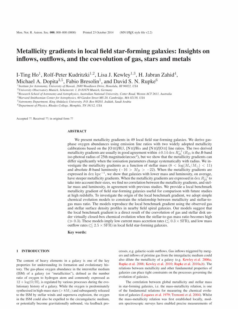
Figure 1. An example of the spectral fitting approach applied on the CALIFA data (see Section 3.1 for details). The grey and black thick lines in the upper
panel indicate the wavelength ranges where the data (black: V500 data; grey: V1200 data) are adopted to constrain the continuum models (red: V500; pink:
V1200). Bad channels, the vicinity of strong emission lines and sky lines are excluded from the fit. The four middle panels show emission lines (red) fit to the
continuum subtracted spectra (black). All lines are fit simultaneously and share the same velocity and velocity dispersion. The bottom four panels show the
residuals, and the blue dashed lines indicate the ±1σ noise levels.
lines, [O II] λλ3726,3729, Hβ, [O III] λ5007, [O I] λ6300, Hα,
[N II] λ6583, and [S II] λλ6716,6731.
All the 9 galaxies analysed in this study have multiple
bright HII regions measured in all the strong lines including
[O II]3726,3729, which allows reliable constraints simultaneously
on metallicity and ionisation parameters with different diagnostics.
2.4 Galaxies from Rupke et al. (2010b)
Rupke et al. (2010b, hereafter R10) measured metallicity gradients
in interacting and non-interacting galaxies. They show that, on av-
erage, interacting systems present shallower metallicity gradients
than non-interacting systems. Their control sample comprises 11
non-interacting local galaxies and they measure their metallicity
gradients using published emission line data from HII regions. Two
of these control sample galaxies overlaps with the S12 sample.
We include their measurements for the remaining 9 galaxies in
our analysis. Their methods of correcting for extinction and de-
riving metallicity are exactly the same as our work and therefore
we include their measurements of metallicity gradients without a
re-analysis of the data.
3 ANALYSIS
3.1 Emission line maps
To place constraints on metallicity and ionisation parameter using
emission line diagnostics, we measure emission line fluxes in each
spaxel of CALIFA and WiFeS galaxies by spectral fitting. We use
an earlier version of the spectral fitting tool LZIFU described in
Ho et al. (in preparation; see also Ho et al. 2014). The fitting ap-
proaches for the two samples are very similar, though some details
are fine tuned to accommodate the differences in spectral coverage
and resolution between the two datasets. Below, we first elaborate
our method for the CALIFA galaxies before describing the different
treatments for the WiFeS galaxies.
Prior to fitting the CALIFA galaxies, we first correct for the
known spatial misalignment between the V500 and V1200 dat-
acubes (Husemann et al. 2013). For each CALIFA galaxy, we re-
align the two cubes by correlating continuum images constructed
separately from the two cubes using a wavelength range covered
by both settings (4240–4620A). Typical misalignments are ∼ 1′′
to 2′′ while in several extreme cases ∼ 3′′ to 5′′. We then rescale
the V1200 data to match the V500 data using scale factors deter-
mined from the median flux density ratios between an overlapped
spectral coverage of 4000A and 4500A. Slight differences in flux
levels may be a result of imperfect calibration and any residual sys-
tematic errors.
We then perform simple stellar population (SSP) synthesis to
remove the underlying stellar continuum before fitting emission
lines. To model the stellar continuum, we adopt the penalised pixel-
fitting routine (PPXF; Cappellari & Emsellem 2004) and employ
the empirical MIUSCAT4 SSP models of 13 ages5 and 4 metallic-
4 http://miles.iac.es/pages/ssp-models.php5 0.06, 0.10, 0.16, 0.25, 0.40, 0.63, 1.00, 1.58, 2.51, 3.98, 6.31, 10.00, and
15.85 Gyr
Metallicity gradients in local field star-forming galaxies 5
NGC7321 Halpha
0 20 40 60R.A. offset [arcsec]
0
20
40
60
Dec
. offs
et [a
rcse
c]
[OII]3726,3729
SDSS composite
E(B−V)
−0.2 0.0 0.2 0.4 0.6
Velocity field
7000 7125 7250 7375[km/s]
O3N2
−0.4 0.0 0.4 0.8
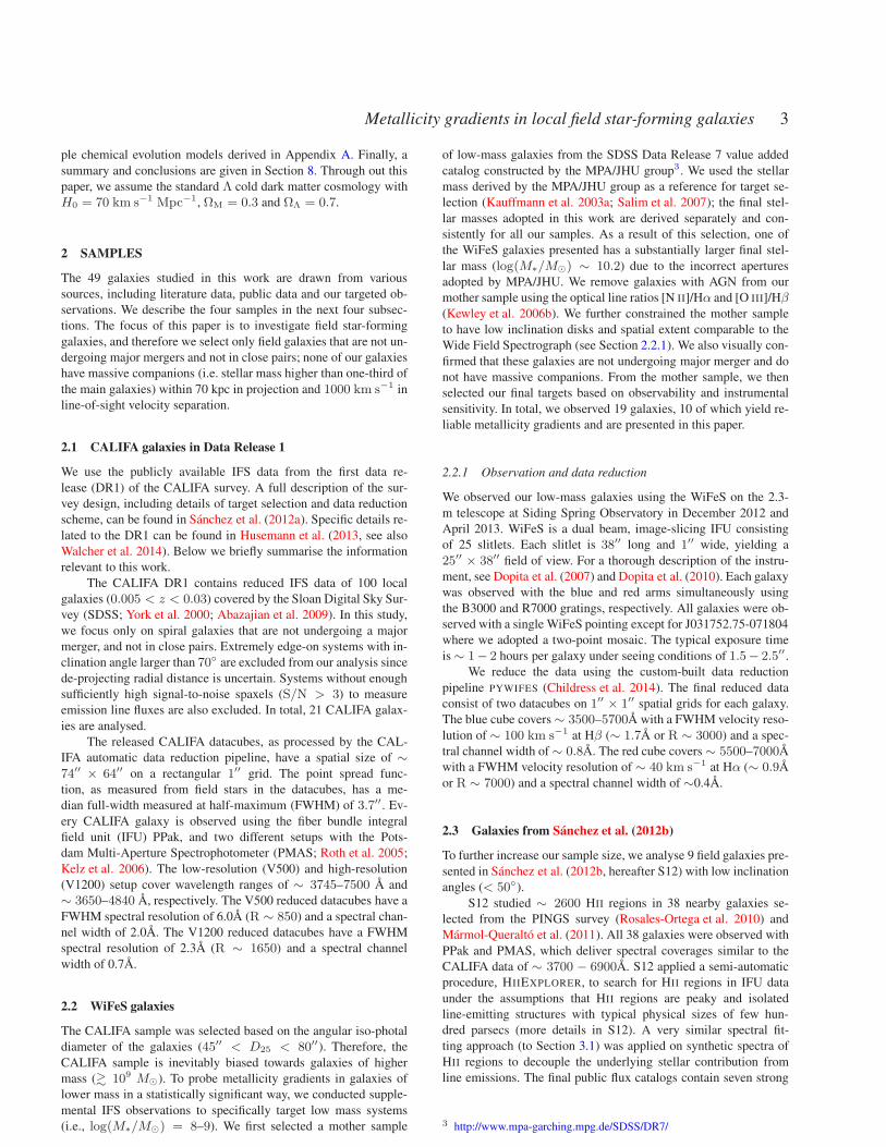
Figure 2. An example of 2D maps from our spectral analysis described in Section 3.1. The first row shows the Hα map, [O II] λλ3726,3729 map, and SDSS
3-colour image of NGC7321, one of the CALIFA galaxies. The second row shows the E(B-V) , velocity field, and O3N2 maps. The bright foreground star in
the SDSS image is masked out in all the other maps.
ities6 (Vazdekis et al. 2010) while assuming a Salpeter initial mass
function (IMF; Salpeter 1955). Bad pixels, sky lines and the vicin-
ity (±15A) of emission lines are masked prior to fitting the con-
tinuum models. After subtracting the continuum models from the
data, we further remove low frequency fluctuations in the residuals
by fitting fourth order b-spline models. We note that the major goal
of performing SSP synthesis fitting is to correct for stellar Balmer
absorption; we do not derive stellar age and metallicity from our
SSP fits.
Subsequent to removing the continuum in the V500 and
V1200 datacubes separately, we model the strong emission lines
([O II] λλ3726,39, Hβ, [O III] λλ4959,5007, [N II] λλ6548,6583,
Hα, and [S II] λλ6716,6731) as simple gaussians. We perform
a bounded value nonlinear least-squares fit using the Levenberg-
Marquardt method implemented in IDL (Markwardt 2009, MP-
FIT). We constrain (1) all lines to have the same velocity and
velocity dispersion, (2) the ratios [N II] λ6583/[N II] λ6548 and
[O III] λ5007/[O III] λ4959 to their theoretical values given by
quantum mechanics, (3) the velocity to be between +600 km s−1
and −600 km s−1 to the systemic velocities as measured from
SDSS, and (4) the velocity dispersion to be between 50 and 1000
km s−1.
Figure 1 shows a typical spectrum and spectral fit. This fig-
6 [M/H] = -0.71, -0.40, 0.00, and 0.22
ure best illustrates the above procedure of decoupling stellar con-
tribution in each spaxel from emission lines originated predomi-
nantly from HII regions. Figure 2 shows two emission line maps,
SDSS composite image, extinction map, velocity field map, and a
key diagnostics line-ratio map of the CALIFA galaxy NGC7321 to
demonstrate the final products from our analysis described above.
For fitting the WiFeS galaxies, the above procedure is adopted
with some minor modifications to accommodate the different spec-
tral coverages and resolutions. No correction for misalignment is
required for the WiFeS datacubes since the blue and red data were
observed simultaneously. SSP synthesis fitting is performed simul-
taneously on both cubes to take full advantage of the 4000A break,
an important age indicator, captured only in the blue data. Fitting
the red side separately would in principle increase the degenera-
cies in SSP synthesis fitting. We first down-grade the red data to
the same spectral resolution as the blue data (R ∼ 3000), mask
out noisy parts of the spectra due to poor CCD sensitivities, and
merge the two datacubes to form a master datacube which covers
∼ 3700–6950A. We then use PPXF and theoretical SSP models,
assuming Padova isochrones, of 18 ages7 and 3 metallicities8 from
Gonzalez Delgado et al. (2005) to determine the contribution from
7 0.004, 0.006, 0.008, 0.011, 0.016, 0.022, 0.032, 0.045, 0.063, 0.089,
0.126, 0.178, 0.251, 0.355, 0.501, 0.708, 1.000, and 1.413 Gyr.8 Z = 0.004, 0.008, and 0.019.
6 Ho et al.
different stellar populations and the degree of dust extinction. The
results are then used to reconstruct continua of the blue and red data
at their native spectral resolution. The same line fitting approach is
then applied to the continuum subtracted cubes and yields emission
line maps.
3.2 Extinction correction
We use a consistent method for all the galaxies to correct the
wavelength-dependent extinction caused by dust attenuation. For
a given measurement (i.e., a spaxel for the CALIFA and WiFeS
samples or an HII region for the S12 samples), we assume the
classical extinction law by Cardelli et al. (1989) with Rv = 3.1and Hα/Hβ = 2.86 under the case-B recombination of Te =10, 000 K and ne = 100 cm−3 (Osterbrock & Ferland 2006). This
prescription is consistent with that adopted in R10.
3.3 Other physical quantities
3.3.1 Stellar mass (M∗)
We use the LE PHARE9 code developed by Arnouts, S. & Ilbert,
O. to estimate the galactic stellar mass. LE PHARE compares pho-
tometry measurements with stellar population synthesis models,
based on a χ2 template-fitting procedure, to determine mass-to-
light ratios, which are then used to estimate the stellar mass of
galaxies. The stellar templates of Bruzual & Charlot (2003) and
a Chabrier IMF (Chabrier 2003) are used to synthesise magni-
tudes. The 27 models span three metallicities and seven expo-
nentially decreasing star formation models (SFR ∝ e−t/τ ) with
τ = 0.1, 0.3, 1, 2, 3, 5, 10, 15 and 30 Gyr. We apply the dust atten-
uation law from Calzetti et al. (2000) allowing E(B − V ) to vary
from 0 to 0.6 and stellar population ages ranging from 0 to 13 Gyr.
Photometric measurements are collected from various
sources. For all the 21 CALIFA galaxies, 10 WiFeS galaxies, and
5/9 S12 galaxies, we adopt values from the SDSS DR7 photometry
catalog (Abazajian et al. 2009) and 2MASS extended source cata-
log (Skrutskie et al. 2006). The Petrosian magnitudes of SDSS u, g,
r, i, and z-band are corrected for the foreground Galactic-extinction
(Schlegel et al. 1998). The 2MASS J, H, and Ks magnitudes mea-
sured from fit extrapolation are adopted to approximate the total
magnitudes. All these galaxies have the 5-band SDSS photometry
and the majority (28/36) also have the 3-band 2MASS photometry.
For the rest of the four S12 galaxies and the nine R10 galaxies, we
collect available U, B, V, and the 3-band 2MASS photometric mea-
surements from NASA/IPAC Extragalactic Database (NED). All
these galaxies have the 3-band 2MASS photometry. The B and V-
band photometry are available for all galaxies, and the U-band pho-
tometry is available for about half of these galaxies (6/13). These
optical photometric measurements are also corrected foreground
Galactic-extinction. When reasonable uncertainties of the measure-
ments are unavailable, we assume 0.1 dex for the optical bands and
0.05 dex for the infrared bands.
We note that the uncertainties in stellar mass are typically
dominated by systematic errors. Different stellar mass estimators
employ different algorithms and stellar libraries, but the estimated
M∗ typically agrees within ∼ 0.3 dex, marking the degree of
systematic errors in the measurements (e.g., Drory et al. 2004;
Conroy et al. 2009).
9 http://www.cfht.hawaii.edu/ arnouts/LEPHARE/lephare.html
3.3.2 Inclination angle
Inclination angles of CALIFA galaxies are estimated using the con-
version provided by Padilla & Strauss (2008). The effects of dust
extinction and reddening were taken into account in their analysis.
An estimate of inclination angle for spiral galaxy is inferred from
the measured axis ratio (b/a) and r-band absolute magnitudes.
Axis ratios estimated by the CALIFA team from SDSS r-band im-
ages are adopted. Inclination angles of WiFeS galaxies are drawn
from Hyperleda (Paturel et al. 2003), which assumes the classical
Hubble formula (Hubble 1926). Inclination angles of S12 galaxies
are taken directly from table 1 in S12, which also refers to values
from Hyperleda. Inclination angles of R10 galaxies are taken di-
rectly from table 2 in R10, which is a compilation from various
references.
3.3.3 Size and distance
We compile the sizes and distances of our samples from NED and
Hyperleda. R25 from Hyperleda is adopted throughout the paper to
quantify sizes of the galaxies. Redshift independent distances are
available for all R10 galaxies in Table 2 of R10. Redshift indepen-
dent distances for most S12 galaxies (7/10) are adopted from NED.
These redshift independent distances (d . 30 Mpc) are measured
from the Tully-Fisher relation, tip of the red-giant brach method,
planetary nebulae, type-II supernovae, or Cepheid variables. For
CALIFA, WiFeS, and the rest of the three S12 galaxies, we adopt
Hubble distances inferred from their redshifts.
4 DERIVATION OF METALLICITIES AND
METALLICITY GRADIENTS
In this section, we describe our methodology for using emission
line ratios to derive metallicities, metallicity gradients and ionisa-
tion parameters.
4.1 Metallicity
The most direct way to determine an ISM metallicity is by first
measuring electron temperatures (Te) with temperature sensitive
line ratios, e.g., [O III] λ4363 to [O III] λ5007, and then convert
emission measures to metallicity after correcting for unseen stages
of ionisation. Since [O III] λ4363 is typically unavailable or only
detected in very limited (i.e. the hottest) regions in IFU surveys,
measuring metallicity usually relies on empirical or theoretical cal-
ibrations (or a combination of both) based on strong emission lines,
such as those available in our samples. Various such calibrations are
available in the literatures and are widely adopted to derive metal-
licity (e.g., Kewley & Dopita 2002; Pettini & Pagel 2004).
We drive metallicities with two different calibrations elabo-
rated below. Throughout the paper, we express the metallicity is in
terms of the number ratio as 12 + log(O/H).
4.1.1 O3N2 index / PP04
The O3N2 index, defined as
O3N2 ≡ log[O III] λ5007/Hβ
[N II] λ6583/Hα, (1)
is a widely used metallicity diagnostic in the literature. An em-
pirical calibration is provided by Pettini & Pagel (2004, hereafter

Metallicity gradients in local field star-forming galaxies 7
PP04). The popularity of this diagnostics arises for two reasons.
Firstly, the four lines involved are usually easily measured in lo-
cal galaxies out to large radii using modern instruments. Secondly,
because of the minimum wavelength differences between the two
pairs of lines, the O3N2 index is virtually free from systematics
caused by the assumption of an extinction law or reddening uncer-
tainties. Nevertheless, the calibration provided by Pettini & Pagel
(2004) is calibrated empirically with a linear fit to metallicities of
137 extragalactic HII regions (131 with Te-based metallicity and 6
with detailed photoionisation models). Variation of ionisation pa-
rameter, q, is not considered in the calibration. Neglect of this pa-
rameter may cause serious systematic errors in the results.
4.1.2 N2O2 index / KD02
The N2O2 index, defined as
N2O2 ≡ log[N II] λ6583
[O II] λλ3726,3729, (2)
is an alternative metallicity diagnostic that has been calibrated by
Kewley & Dopita (2002, hereafter KD02) using theoretical pho-
toionisation models. We adopt the parametrisation for q = 2 ×107cm s−1 in KD02 to derive metallicity. The N2O2 index is in-
sensitive to variation of ionisation parameter by virtue of the sim-
ilar ionising potential of N+ and O+. Despite the insensitivity to
ionisation parameter, N2O2 is not often used in local studies pri-
marily because some spectrographs are not sensitive enough at
∼ 3700A to observe [O II] λ3726,3729. The N2O2 calibration
depends more on the assumed extinction law and extinction esti-
mate than O3N2 due to the larger wavelength separation between
[N II] λ6583 and [O II] λλ3726,3729. We note that the variation
in the N/O ratio with O/H could be the largest uncertainty affect-
ing these strong line diagnostics (Henry et al. 2000). The strength
of the [O II] λ3726,3729 lines are strongly affected by the electron
temperature, governed predominately by the O/H ratio and ionisa-
tion parameter, while [O III] λ5007 is mostly sensitive to the ioni-
sation parameter.
A long standing problem in chemical studies has been that
different metallicity calibrations do not return consistent metal-
licity measurements. Kewley & Ellison (2008) applied 10 differ-
ent metallicity calibrations on the same SDSS dataset and found
that different calibrations yield different mass-metallicity relations.
Both the slopes and the intercepts of the mass-metallicity relation
are significantly different from calibration to calibration. By allow-
ing the mass-metallicity relations derived with different calibra-
tions to be converted to the same bases, Kewley & Ellison (2008)
derived empirical conversions between different calibrations. In
this paper, metallicities derived using the O3N2 method are sub-
sequently converted to the KD02 scale using the conversion by
Kewley & Ellison (2008).
We note that, when deriving metallicities using a certain diag-
nostic, we only use data with S/N > 3 on all the lines associated to
that particular diagnostic. The same rule also applies to the deriva-
tion of the ionisation parameter (see Section 4.3).
4.2 The importance of non-thermal excitation and diffuse
ionised gas
It is important to understand that all the above metallicity diag-
nostics are calibrated empirically or theoretically using HII re-
gions. This means, by applying the diagnostics, one implicitly
103 104 1050.8
0.6
0.4
0.2
0.0
103 104 105
Ha flux (arbitrary)
0.8
0.6
0.4
0.2
0.0
[SII]
/Ha
0.2
0.4
0.6
0.8
1.0
1.2
1.4
CH
II
Figure 3. An Example of determining spaxels heavily contaminated by the
diffuse ionised gas. Details are described in Section 4.2. The black points
are all star-forming spaxels with> 3σ detections on the [S II]λλ6716,6731
and Hα lines. The blue and red squares are those spaxels with > 3σ de-
tections on all lines associated with the O3N2 index, i.e., [O III] λ5007,
[N II] λ6583, Hα, and Hβ. The green curve indicates the best fit to the
black points using equations 3 and 4, which we adopt to determine the crit-
ical Hα flux above which the covering fraction of HII region exceeds 80%.
Data below the critical Hα flux (red) are excluded from deriving O3N2
metallicity.
assumes that that all the nebular emission originates from pho-
toionisation and heating caused by the extreme ultraviolet pho-
tons emitted by O and B-type stars. If other ionisation sources
are present, metallicity measurements would be contaminated.
Other ionisation sources such as active galactic nuclei (AGNs)
can have localised or even global effects on line ratios. Interstel-
lar shocks originating from AGN outflows, supernovae, or stel-
lar winds are also sources of non-thermal radiation and can af-
fect emission line ratios. To remove measurements affected by
non-thermal radiation from our subsequent analyses, we use line
ratio diagnostics commonly adopted to distinguish normal from
active galaxies (i.e., [O III] λ5007/Hβ v.s. [N II] λ6583/Hα or
BPT diagram; Baldwin et al. 1981; Veilleux & Osterbrock 1987).
We adopted the empirically separation line derived from SDSS
by Kauffmann et al. (2003b, hereafter K03; see also Kewley et al.
2001 and Kewley et al. 2006b) to exclude data contaminated by
non-thermal excitation.
Emission from the diffuse ionise gas (DIG; also known as
the warm ionised medium) can be a non-negligible component
in IFU measurements. The DIG is hot (∼ 104 K) and tenuous
gas (∼ 10−1 cm−3) permeating the interstellar space and extend-
ing more than 1 kpc above the disk plane (see Mathis 2000 and
Haffner et al. 2009 for reviews). The DIG generally presents much
lower Hα surface brightness than typical HII regions and displays
distinctly different line ratios from HII regions. The primary ex-
citation sources are thought to be predominately ionising photons
escaping and traveling kilo-parcsec distances from O and B-type
stars. Measurements in an IFU spaxel can contain both emission
from underlying HII regions and from the DIG along the line-of-
sight.
To quantify the fractional contributions from the DIG and
HII regions in a given spaxel, we adopt a similar approach as
Blanc et al. (2009). Spaxels dominated by the DIG are subse-
quently removed from our analyses. We constrain the contribution

8 Ho et al.
0.0 0.2 0.4 0.6 0.8 1.0 1.2 1.4deproj. radius[R25]
8.0
8.5
9.0
9.5
12+
log(
O/H
) O
3N2
0 5 10 15deproj. radius [kpc]
CALIFA:NGC4210
0.0 0.2 0.4 0.6 0.8 1.0 1.2 1.4deproj. radius [R25]
8.0
8.5
9.0
9.5
12+
log(
O/H
) N
2O2
0 5 10 15deproj. radius [kpc]
0.0 0.2 0.4 0.6 0.8 1.0 1.2 1.4deproj. radius [R25
7.07.27.47.67.88.08.2
log(
q) [c
m/s
]
0 5 10 15deproj. radius [kpc]
0.0 0.2 0.4 0.6 0.8 1.0 1.2 1.4deproj. radius[R25]
8.0
8.5
9.0
9.5
12+
log(
O/H
) O
3N2
0 5 10 15deproj. radius [kpc]
CALIFA:UGC03253
0.0 0.2 0.4 0.6 0.8 1.0 1.2 1.4deproj. radius [R25]
8.0
8.5
9.0
9.5
12+
log(
O/H
) N
2O2
0 5 10 15deproj. radius [kpc]
0.0 0.2 0.4 0.6 0.8 1.0 1.2 1.4deproj. radius [R25
7.07.27.47.67.88.08.2
log(
q) [c
m/s
]
0 5 10 15deproj. radius [kpc]
Figure 4. Left and middle panels: Metallicity gradients of individual CALIFA galaxies measured using the two different abundance diagnostics (see Sec-
tion 4.1). The straight lines indicate the best fits, and the dashed lines indicate ±1σ errors. The errors of the intercepts and the slopes are estimated from
bootstrapping (see Section 4.4). Right panels: ionisation parameter as a function of radius. The ionisation parameters are derived using the [O III]/[O II] diag-
nostic (KK04; see Section 4.3). Each point in these plots corresponds to one IFU spaxel with significant (> 3σ) detections on all the emission lines associated
with the diagnostics. Spaxels contaminated by non-thermal excitation or dominated by DIG emission are rejected (see Section 4.2). The vertical dashed lines
correspond to the radial cutoff within which the data are not considered in constraining the disk metallicity gradients.
from the DIG with the observed the observed [S II]/Hα ratio
[S II]
Hα= Z′
[
CHII([S II]
Hα)HII +CDIG(
[S II]
Hα)DIG
]
, (3)
where [S II] denotes the total flux of [S II] λ6716 and [S II] λ6731.
The terms CHII and CDIG represent fractions of emission lines
originated from HII regions and the DIG, respectively. The sum of
CHII and CDIG is unity. Z′ denotes metallicity of the galaxy nor-
malised to that of the Milky Way, i.e. Z′ = Z/ZMW . Following
Blanc et al. (2009), we adopt the value of ([S II]/Hα)HII as 0.11
and ([S II]/Hα)DIG as 0.34. These values are supported by obser-
vations of HII regions and the DIG in our Milky Way (Madsen et al.
2006).
Figure 3 shows a typical [S II]/Hα versus Hα flux plot of the
CALIFA galaxy NGC6497. All the data points (spaxels) are sig-
nificantly detected (> 3σ) in [S II] and Hα. Spaxels with high Hαfluxes have low (high) [S II]/Hα, consistent with the low (high)
line ratios of HII regions (DIG). HII regions are generally located
on spiral arms and DIG is generally located in inter-arm regions.
Similar to Blanc et al. (2009), we model the covering fractions
of HII regions in each galaxy as a simple function of
CHII = 1−f0
f(Hα), (4)
where f(Hα) is the Hα flux. Combining equation 3 and equation 4,
we fit simultaneously Z′ and f0, and show the best fit as the green
curve in Figure 3. We typically find equation 4 describes the data
reasonably well, but the theoretical basis of this functional form
is unclear. The best fit provides a guide for imposing a criterion
on the Hα flux to reject spaxels below a characteristic covering
fraction of HII regions. We exclude all spaxels below an Hα flux
value at which the corresponding CHII is 0.8 on the best fit curve.
Although this criterion seems arbitrarily strict, changing the char-
acteristic covering fraction to zero has only a minor impact on the
metallicity gradients of individual galaxies, and none of our con-
clusions change.
The reason that rejecting DIG dominated spaxels has limited
effect is that the covering fraction cut does not remove many spax-
els that have not already been rejected by the S/N cuts for metal-
licity diagnostics and the BPT criterion (K03) for non-thermal ex-
citation. The strictest criteria in rejecting the data are the S/N cuts
on the weak lines such as Hβ and [N II] λλ6548,6583. Since the
DIG has intrinsically low surface brightness, with the current depth
in CALIFA and WiFeS samples, most spaxels satisfying multiple
S/N > 3 criteria in line emissions are those with low DIG cov-
ering fractions. We demonstrate this in Figure 3. The blue and red
points are the spaxels satisfying the S/N > 3 criteria in the O3N2
diagnostic and the criterion on the BPT (K03). The red points are
those further rejected by the DIG criterion.
We note that rejecting data dominated by the DIG is only re-
quired for spaxel-to-spaxel analysis, i.e. the CALIFA and WiFeS
samples. For the S12 galaxies, the fluxes were measured on ex-
tracted spectra of HII regions (i.e., binning spaxels in the vicinity
of bright and compact Hα knots). For R10, the flux measurements
were performed by placing long-slits on HII regions. DIG contam-
ination is expected to be negligible in these two cases.
In principle, after the fractional contribution is determined,
one should be able to subtract the contribution from the DIG and
derive the fluxes from underlying HII regions (as in Blanc et al.
2009). However, line ratios involving [O II] λλ3726,3729 for the
DIG are not well constrained and could produce large scatter (e.g.,
[O II] λλ3726,3729/Hα; Mierkiewicz et al. 2006). Even for the
well-measured ratios, such as [S II]/Hα and [N II]/Hα, considerable
scattering and correlation between [S II]/[N II] could complicate the
corrections and induce potential systematic errors (Madsen et al.
2006). In this work, we adopt the simplest approach of rejecting
inappropriate data. Comprehensive theoretical modelling and ob-
servational constraints of DIG are crucial for extracting more in-
formation from deeper IFU data.
4.3 Ionisation parameter
The ionisation parameter is quantified as the ionising photon flux
through a unit area divided by the local number density of hydro-
gen atoms. The ionisation parameter can be measured by taking
the ratio of high ionisation to low ionisation species of the same
atom. Using the strong lines available in this study, we measure

Metallicity gradients in local field star-forming galaxies 9
0.0 0.2 0.4 0.6 0.8 1.0 1.2 1.4deproj. radius[R25]
8.0
8.5
9.0
9.5
12+
log(
O/H
) O
3N2
0 5 10 15 20deproj. radius [kpc]
S12:NGC3184
0.0 0.2 0.4 0.6 0.8 1.0 1.2 1.4deproj. radius [R25]
8.0
8.5
9.0
9.5
12+
log(
O/H
) N
2O2
0 5 10 15 20deproj. radius [kpc]
0.0 0.2 0.4 0.6 0.8 1.0 1.2 1.4deproj. radius [R25
7.07.27.47.67.88.08.2
log(
q) [c
m/s
]
0 5 10 15 20deproj. radius [kpc]
0.0 0.2 0.4 0.6 0.8 1.0 1.2 1.4deproj. radius[R25]
8.0
8.5
9.0
9.5
12+
log(
O/H
) O
3N2
0 5 10 15 20deproj. radius [kpc]
S12:UGC06410
0.0 0.2 0.4 0.6 0.8 1.0 1.2 1.4deproj. radius [R25]
8.0
8.5
9.0
9.5
12+
log(
O/H
) N
2O2
0 5 10 15 20deproj. radius [kpc]
0.0 0.2 0.4 0.6 0.8 1.0 1.2 1.4deproj. radius [R25
7.07.27.47.67.88.08.2
log(
q) [c
m/s
]
0 5 10 15 20deproj. radius [kpc]
Figure 5. Same as Figure 4, but for the S12 galaxies. Each point corresponds to one HII region extracted from the IFU data (see Section 2.3 and S12 for
details).
the ionisation parameter using [O III] λ5007/[O II] λλ3726,3729
(hereafter, [O III]/[O II]). A theoretical calibration was first pre-
sented in KD02 and a more user-friendly parametrisation is given
in Kobulnicky & Kewley (2004, hereafter KK04). The latter is
adopted in this paper. As emphasised in KD02, in addition to ion-
isation parameter, the [O III]/[O II] ratio also strongly depends on
metallicity that needs to be known a priori. We adopt the metallic-
ity from the N2O2 calibration to derive the ionisation parameter for
each spectrum.
4.4 Measuring metallicity gradients
To derive metallicity gradients, we first convert the flux ratios to
metallicities. For bulge-dominated galaxies or those with obvious
bar structures in the CALIFA sample, we do not include data within
(0.1–0.2) × R25. At the centres of these generally high-mass sys-
tems, the optical spectrum is dominated by the stellar continuum
with strong Balmer absorption originating from an old stellar popu-
lation. Correcting for Balmer absorptions in these regions is less ro-
bust and more sensitive to both the SSP models and the algorithms
adopted (e.g., Cid Fernandes et al. 2014, and references therein).
The WiFeS galaxies do not suffer from this contamination because
these low-mass systems are typically emission dominated even at
the centres. The S12 and R10 galaxies also do not suffer from this
artefact because the emission lines are directly measured towards
HII regions.
To estimate the errors in the metallicity gradients, we
adopt a bootstrapping approach similar to Kewley et al. (2010),
Rupke et al. (2010b) and Rich et al. (2012). We randomly draw
from the measurements the same number of data points but with re-
placement, and perform an unweighted least-squares linear fit with
the drawn data. In each galaxy, this process is repeated 1,000 times
and each fit result is recorded. The median and standard deviation
of the slopes and intercepts are considered as the best estimates of
the metallicity gradient.
5 RESULT
5.1 Metallicity gradients of individual galaxies
In Figure 4 and Figure 5, we present 4 metallicity gradients mea-
sured in two CALIFA and two S12 galaxies, respectively. The two
different metallicites are shown in the first two panels, and the last
panels show radial profiles of the ionisation parameter. In the first
two panels, straight lines indicate the best fits of the gradients, and
dashed lines indicate 1σ errors as propagated using analytic ex-
pressions with bootstrapped errors. The rest of the CALIFA and
S12 galaxies are presented in Figures B1 and B2 in Appendix B.
The metallicity gradients and the radial profiles of the ionisa-
tion parameter of our 10 WiFeS galaxies are also presented in Fig-
ure B3. The metallicity of the majority of WiFeS galaxies falls into
a regime where the conversion from O3N2 to N2O2 behaves poorly
(12 + log(O/H) < 8.4 in KD02 scale), and therefore we are only
able to derive their N2O2 metallicity gradients. These galaxies are
excluded from the rest of the comparisons between two metallicity
−1.0 −0.8 −0.6 −0.4 −0.2 0.0 0.2N2O2 metallicity gradient [dex R25
−1 ]
−1.0
−0.8
−0.6
−0.4
−0.2
0.0
0.2
O3N
2 m
etal
licity
gra
dien
t [de
x R
25−1 ]
UGC06410
NGC3184
NGC4210
UGC03253
S12CALIFA+/− 0.14+/− 0.05
x=y
Figure 6. Left: Comparison between the metallicity gradients (dex R−125 )
derived using the O3N2 and the N2O2 diagnostics (see Section 4.1). The
metallicity gradients of the majority of the galaxies (33%/73%) agree within
±0.05/±0.14 dex R−125 . The metallicity gradients of the four outliers la-
beled are shown in Figure 4 and Figure 5.

10 Ho et al.
calibrations, but we include them later while comparing metallicity
gradients of different galaxies (Section 5.4).
In Figure 6, we compare metallicity gradients derived
from O3N2 and from N2O2 for the CALIFA and S12 galax-
ies. All the galaxies exhibit negative metallicity gradients in
both calibrations, and 33%/73% of the galaxies agrees within
±0.05/±0.14 dex R−125 . These values can be considered as the
level of residual systematics in the metallicity calibrations. Notice-
ably there are several outliers well below the one-to-one line which
we label in Figure 6. These objects could provide insight into the
cause of the disagreement between the two calibrations. We fur-
ther investigate the cause of this discrepancy in the following two
subsections.
5.2 The effect of ionisation parameter
In the left panel of Figure 7, we compare the metallicities derived
using the O3N2 and N2O2 calibrations. Each point represents one
measurement, i.e., one spaxel from the CALIFA galaxies or one HII
region from the S12 galaxies. We colour-code the points by log(q)
derived using the [O III]/[O II] (KK04) calibration. The left panel
of Figure 7 clearly demonstrates that superficially the two metal-
licities agree reasonably well; 57%/83% of the metallicities agree
within ±0.05/0.1 dex. Similar comparisons were also carried out
by Rupke et al. (2010b) where comparable scattering also exists.
In the left panel of Figure 7, the scattering around the one-
to-one line is not random, but correlates with ionisation param-
eter. Spaxels or slits with high ionisation parameter have higher
N2O2 metallicities than O3N2 metallicities. Those with low ion-
isation parameter have lower N2O2 metallicity than O3N2 metal-
licities. In the right panel of Figure 7, we show the difference be-
tween metallicities derived with the O3N2 and N2O2 ratios ver-
sus ionisation parameter. The differences between the two diag-
nostics can be up to 0.2 – 0.4 dex at extreme values of ionisa-
tion parameter (log(q) < 7.0 cm s−1 or log(q) > 8.2 cm s−1
). At log(q) & (.)7.3 cm s−1, the O3N2 diagnostic gives higher
(lower) metallicity than the N2O2 diagnostic. Clearly, ionisation
parameter is the cause of the discrepancy. As we emphasised ear-
lier, O3N2 is calibrated empirically without taken into account the
change of ionisation parameter. A theoretical calibration of O3N2
will be presented in Kewley et al. (in preparation) and will rec-
oncile this discrepancy with new stellar population synthesis and
photoionisation models.
5.3 Discrepancies among metallicity gradients
We now return to discuss the cause of the discrepancies in the
metallicity gradients shown in Figure 6.
Figure 4 (and Figure 5) show metallicity gradients for two
CALIFA (two S12 galaxies) that are labeled as outliers in Figure 6.
These galaxies have steeper O3N2 than N2O2 metallicity gradients
because, at large radii, O3N2 metallicities are systematically lower
than N2O2 metallicities. As shown in Figure 7, lower O3N2 than
N2O2 metallicities naturally arises when log(q) & 7.3 cm s−1.
Indeed in the third panels of Figure 4 and Figure 5, these galaxies
typically have log(q) & 7.3 cm s−1 at large radii. These galax-
ies all show indications of smooth rising of ionisation parameter
from their centres to outskirts, implying a continuous radial change
of their properties of the ionising radiation. The higher ionisation
parameters could be caused by the more active star formation ac-
tivities with different distributions of molecular gas (Dopita et al.
2014).
In extreme cases, the differences in metallicity gradient mea-
sured with N2O2 and O3N2 can be up to a ∼ 0.4 dex R−125
(e.g., NGC3184 in Figure 5). Similar findings are also reported
in Rupke et al. (2010b). These results have important implica-
tions for metallicity gradient studies at high redshift, where typ-
ically only [N II] λλ6548,6583 and Hα are available (in some
cases also [O III] λλ4959,5007 and Hβ, e.g., Cresci et al. 2010;
Yuan et al. 2011; Jones et al. 2010, 2013; Queyrel et al. 2012;
Swinbank et al. 2012). While all the diagnostics using these four
lines, i.e. [N II] λ6583/Hα and O3N2, are sensitive to the change of
ionisation parameter, quantitative interpretation of metallicity gra-
dients should bear in mind the potential impact of ionisation pa-
rameter gradients in galaxies.
For galaxies not labeled in Figure 6, we do not find obvious
signs of a correlation between ionisation parameter and radius. The
inconsistency in metallicities derived using the O3N2 and N2O2
diagnostics does not correlate with radius. When measuring metal-
licity gradients in these galaxies, the net effect is merely to increase
the uncertainties in the measurements, rather than biasing the mea-
surements in any systematic way. This is essentially the cause of
the small scatter (. 0.1 dex R−125 ) in Figure 6.
5.4 Metallicity gradients in field star-forming galaxies
After investigating the systematics induced by the variation of ion-
isation parameter, we adopt the N2O2 measurements as our final
metallicity gradients and we now compare metallicity gradients in
field star-forming galaxies with their stellar mass and B-band lumi-
nosity.
5.4.1 Metallicity gradient - stellar mass
The upper and lower panels of Figure 8 show the metallicity gradi-
ent versus stellar mass of our four samples in units of dex kpc−1
and dexR−125 , respectively. In the upper panel, the metallicity gradi-
ents appear to depend on stellar mass where (1) low mass galaxies
have on average a steeper metallicity gradient, and (2) are more
diverse in the steepness of metallicity gradients compared to high-
mass galaxies. To quantify the dependency, we split the sample into
two mass bins with roughly equal numbers of galaxies, i.e. a high-
mass bin (log(M∗/M⊙) > 9.6; Ngal = 24) and a low-mass bin
(log(M∗/M⊙) < 9.6; Ngal = 25). We compute the bootstrapped
means and standard deviations of the metallicity gradients. The re-
sults are tabulated in Table 1. We indeed find that the low-mass
galaxies have a steeper mean metallicity gradient at 3.4σ level than
the high-mass galaxies, and also a larger standard deviation of the
metallicity gradients at 3.7σ level.
When the metallicity gradients are normalised to the galaxy
sizes (i.e. dex R−125 ), the lower panel of Figure 8 does not support
any clear dependency of metallicity gradient on stellar mass. The
difference between the means is only at 1.2σ level, with low-mass
galaxies having slightly flatter metallicity gradients than high-mass
galaxies. The standard deviations of the metallicity gradients are
virtually identical (the difference is only 0.6σ).
The different dependency of metallicity gradient on stellar
mass while measuring the metallicity gradient in absolute scale
(kpc) or relative scale (R25) can be understood as a size effect. If
galaxies with steeper dex kpc−1 metallicity gradients are smaller
in their physical sizes (smallR25), then the steep dex kpc−1 metal-
licity gradients would be compensated when the galaxy sizes are
taken into account. Figure 9 shows the dex kpc−1 metallicity
Metallicity gradients in local field star-forming galaxies 11
8.2 8.4 8.6 8.8 9.0 9.2N2O2 12+log(O/H)
8.2
8.4
8.6
8.8
9.0
9.2
O3N
2 12
+lo
g(O
/H)
6.8 7.0 7.2 7.4 7.6 7.8 8.0 8.2log(q) [cm/s]
S12CALIFA
+/− 0.1 dex+/− 0.05 dex
x=y
7.0 7.2 7.4 7.6 7.8 8.0 8.2log(q) [cm/s]
−0.4
−0.2
0.0
0.2
0.4
O3N
2 −
N2O
2 12
+lo
g(O
/H)
S12CALIFA
Figure 7. Left: Comparison between the metallicities derived using the O3N2 and N2O2 diagnostics (see Section 4.1). Each CALIFA data point is an IFU
spaxel, and each S12 data point is an HII region extracted from IFU data. Data points are colour-coded with their corresponding ionisation parameters (see
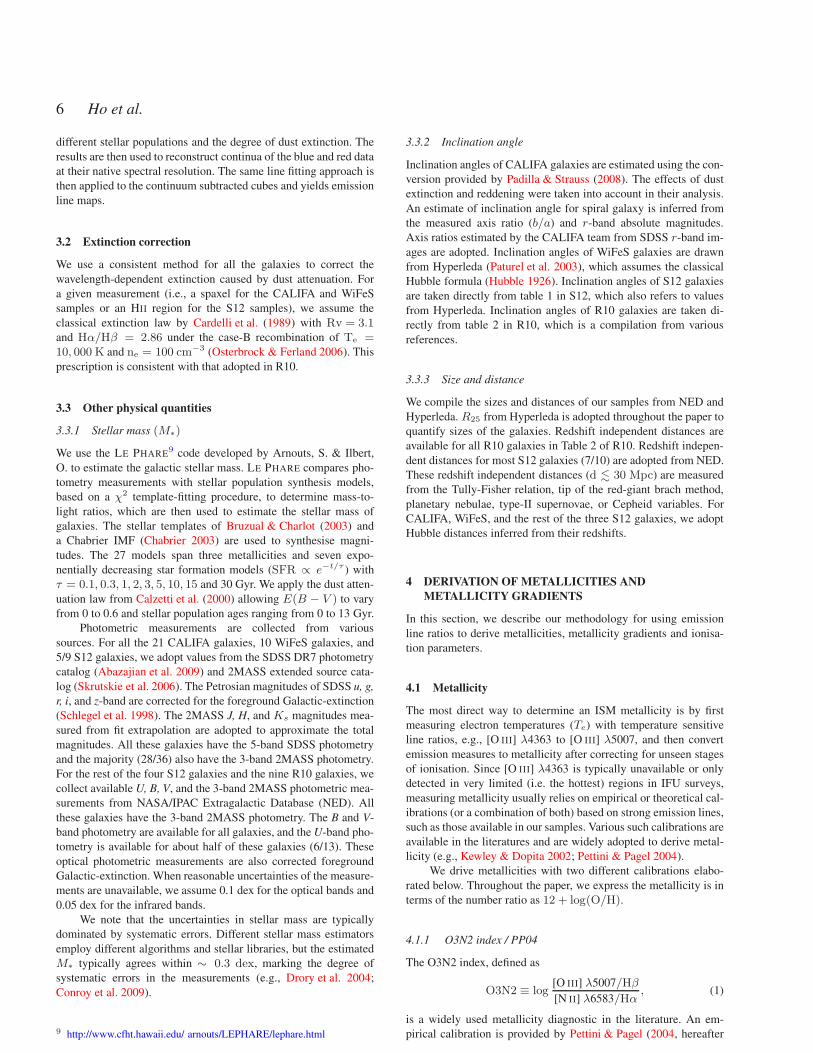
Section 4.3). A total of 57%/83% of the data points agrees within ±0.05/0.1 dex. The degree of disagreement correlates strongly with the ionisation parameter.
Right: Difference between the metallicities derived using the O3N2 and N2O2 diagnostics versus the ionisation parameter. A strong anti-correlation between
the two quantities is obvious. More discussion about this discrepancy of metallicities is provided in Section 5.2, and the impact on measuring metallicity
gradients in Section 5.3.
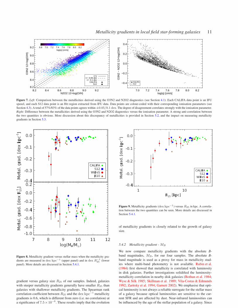
Figure 8. Metallicity gradient versus stellar mass when the metallicity gra-
dients are measured in dex kpc−1 (upper panel) and in dex R−125 (lower
panel). More details are discussed in Section 5.4.1.
gradient versus galaxy size R25 of our samples. Indeed, galaxies
with steeper metallicity gradients generally have smaller R25 than
galaxies with shallower metallicity gradients. The Spearman rank
correlation coefficient between R25 and the dex kpc−1 metallicity
gradients is 0.6, which is different from zero (i.e. no correlation) at
a significance of 7.5×10⁻⁶. These results imply that the evolution
Figure 9. Metallicity gradients (dex kpc−1) versus R25 in kpc. A correla-
tion between the two quantities can be seen. More details are discussed in
Section 5.4.1.
of metallicity gradients is closely related to the growth of galaxy
size.
5.4.2 Metallicity gradient - MB
We now compare metallicity gradients with the absolute B-
band magnitudes, MB , for our four samples. The absolute B-
band magnitude is used as a proxy for mass in metallicity stud-
ies where multi-band photometry is not available. Rubin et al.
(1984) first showed that metallicity is correlated with luminosity
in disk galaxies. Further investigations solidified the luminosity-
metallicity correlation in nearby disk galaxies (Bothun et al. 1984;
Wyse & Silk 1985; Skillman et al. 1989; Vila-Costas & Edmunds
1992; Zaritsky et al. 1994; Garnett 2002). We emphasise that opti-
cal luminosity is not always a reliable surrogate for the stellar mass
of a galaxy because optical luminosities are sensitive to the cur-
rent SFR and are affected by dust. Near-infrared luminosities can
be influenced by the age of the stellar population of a galaxy. Since

12 Ho et al.
Figure 10. Metallicity gradient versus absolute B-band magnitude when
the metallicity gradients are measured in dex kpc−1 (upper panel) and in
dex R−125 (lower panel). More details are discussed in Section 5.4.2.
this quantity is widely adopted in earlier studies, we present our
measurements below for comparison.
In Figure 10, we present metallicity gradient versusMB of our
four samples. Metallicity gradients are shown in both dex kpc−1
(upper panel) and dex R−125 (lower panel). Similarly, we split the
sample into a high luminosity bin (MB < −20.1; Ngal = 24)
and a low luminosity bin (MB > −20.1; Ngal = 25), and com-
pute the bootstrapped means and standard deviations of the metal-
licity gradients (Table 1). We reach the similar conclusions, as in
the comparisons with stellar mass, that (1) low luminosity galax-
ies have a steeper mean dex kpc−1 metallicity gradient (3.4σ),
and (2) low luminosity galaxies have a larger standard deviation
of dex kpc−1 metallicity gradients (3.5σ). When the galaxy sizes
are taken into account, i.e. dex R−125 , the low and high luminos-
ity galaxies have very similar mean metallicity gradients (1.4σ)
and standard deviations (1.8σ). These findings are in agreement
with previous studies (Vila-Costas & Edmunds 1992; Garnett et al.
1997; Prantzos & Boissier 2000).
Few et al. (2012) performed cosmological zoom-in simula-
tions that yield metallicity gradients, disk scale-lengths, B-band
magnitudes, and stellar masses of 19 galaxies in field and loose
group environments. The simulations focused on Milky Way-mass
galaxies spanning stellar mass and B-band magnitude ranges of
10.4 < log(M∗/M⊙) < 11.1 and −19.7 > MB > −21.7, re-
spectively, which correspond to the high-mass and high-luminosity
ends of our samples. Few et al. (2012) found no significant dif-
ferences in metallicity gradients between the galaxies in field
and loose group. The overall metallicity gradients are −0.046 ±
Table 1. A local benchmark gradient
Mean Standard deviation
dex kpc−1
log(M∗/M⊙) > 9.6 −0.026 ± 0.002 0.010± 0.001log(M∗/M⊙) < 9.6 −0.064 ± 0.011 0.054± 0.012
MB < −20.1 −0.025 ± 0.002 0.008± 0.001MB > −20.1 −0.063 ± 0.011 0.053± 0.013
dex R−125
log(M∗/M⊙) > 9.6 −0.42± 0.03 0.16± 0.03log(M∗/M⊙) < 9.6 −0.36± 0.04 0.18± 0.02
MB < −20.1 −0.40± 0.03 0.12± 0.02MB > −20.1 −0.34± 0.03 0.17± 0.02
Alla −0.39a 0.18a
Means, standard deviations and the associated errors are derived from boot-
strapping.aMean and standard deviation of all the galaxies (i.e. not from bootstrap-
ping). See Figure 11.
0.013 dex kpc−1 and −0.40 ± 0.13 dex R−125 (mean ± standard
deviation). Here, we convert the disk scale lengths Rd reported
by Few et al. (2012) to R25 assuming that the exponential disks
have the canonical central surface brightness for normal spirals of
21.65 magnitude/arcsec2 (Freeman 1970). The overall metallicity
gradients by Few et al. (2012) are consistent with our results in the
high-mass and high-luminosity ends. Similar simulations in the fu-
ture targeting lower masses and luminosities could provide valuable
constraints for the different prescriptions built into the simulations.
6 A LOCAL BENCHMARK GRADIENT
We provide a local benchmark of metallicity gradients inspired by
the uniformity of the dex R−125 metallicity gradients. We believe
the local benchmark gradient will be useful for comparison with
metallicity gradients measured at high redshift. In Figure 11, we
present the distribution of the 49 measured metallicity gradients;
and we summarise the mean and standard deviation in Table 1. The
benchmark metallicity gradient measures −0.39 ± 0.18 dex R−125
(mean ± standard deviation). A one-sided Kolmogorov-Smirnov
test yields a 78% probability for the observed distribution to be
drawn from the normal distribution shown as the black curve in Fig-
ure 11. We note that the difference between the O3N2 and N2O2
metallicity gradients is typically 0.14 dex R−125 (Figure 6), compa-
rable to the standard deviation of 0.18 dex R−125 in the benchmark
gradient. This remarkably small difference suggests that the intrin-
sic spread of the metallicity gradients could be even tighter than
0.18 dex R−125 although precisely quantifying the tightness is non-
trivial due to the various systematic effects.
We note that in Figures 8 and 10, the R10 sample appears to
have lower metallicity gradients than the other three samples. A
one-sided Kolmogorov-Smirnov test comparing the R10 sample to
the benchmark gradient, and a two-sided Kolmogorov-Smirnov test
comparing the R10 sample to the whole sample both reveal moder-
ately low but non-zero probability (10%) for the two distributions
to be the same. It is possible that the discrepancy is due to low
number statistics. Furthermore, a two-sided Kolmogorov-Smirnov
test comparing the full sample to that with the R10 galaxies ex-
cluded yields a high probability (99%) for the two distributions to

Metallicity gradients in local field star-forming galaxies 13
Figure 11. Distribution of the 49 metallicity gradients. The overall
mean and standard deviation of the metallicity gradients are −0.39 ±
0.18 dex R−125 (i.e. the benchmark metallicity gradient). The black curve
indicates a Gaussian with these characteristic values, i.e. not a fit to the
distribution. A one-sided Kolmogorov-Smirnov test yields a probability of
78% for the observed distribution to be drawn from the back curve.
be drawn from the same parent distribution. We conclude that the
discrepancy is only apparent and does not change our results.
S12 measured metallicity gradients in 25 face-on spirals and
found a common metallicity gradient of −0.12 ± 0.11 dex R−1e
(median ± standard deviation). Sanchez et al. (2014) expanded
the study to 193 galaxies with the CALIFA survey, and found a very
similar common metallicity gradient of −0.10 ± 0.09 dex R−1e .
Sanchez et al. (2014) showed that, with their large sample size,
the metallicity gradients are independent of morphology, incidence
of bars, absolute magnitude and mass, a result that had also been
hinted by S12. Sanchez et al. (2014) found that the only clear cor-
relation is between merger stage and metallicity gradient, where the
slope is flattened as merger progresses (see also Kewley et al. 2010;
Rupke et al. 2008, 2010a,b; Torrey et al. 2012; Rich et al. 2012).
To compare the common metallicity gradient by Sanchez et al.
(2014) with our benchmark gradient, one must take into ac-
count the different scale-lengths, i.e. Re and R25, and metallic-
ity calibrations (Sanchez et al. 2014 and S12 both adopted the
O3N2/PP04 calibration). Assuming again an exponential disk with
the canonical central surface brightness for normal spirals (i.e.
21.65 magnitude/arcsec2 ; Freeman 1970) and the empirical con-
version between the O3N2/PP04 and N2O2/KD02 metallicities
(Kewley & Ellison 2008), we can convert the common metallicity
gradient by Sanchez et al. (2014) to −0.20±0.18 dexR−125 , which
is about a factor of two shallower than our benchmark gradient.
The difference could be caused by the presence of close pairs and
mergers in their sample. In addition, systematic errors such as the
metallicity calibrations, variations of the ionisation parameter, and
flattening of metallicity gradient at larger radii could all affect the
measured metallicity gradients.
Pilyugin et al. (2014) complied more than 3,000 published
spectra of HII regions and adopted the calibration proposed by
Pilyugin et al. (2012) to measure the metallicity gradients of 130
nearby late-type galaxies. Using 104 of their field spiral galax-
ies (i.e. excluding mergers and close pairs), we constrain a mean
and standard deviation of the metallicity gradients of −0.32 ±0.20 dex R−1
25 . These values are consistent with our benchmark
−1.0 −0.8 −0.6 −0.4 −0.2 0.0 0.2Metal. grad. [dex R−1
25]
0
5
10
15
20
25
Ngal
This work; benchmark gradient
Pilyungin+2014; field spirals
Figure 12. Comparison between our benchmark gradient (dashed curve)
and the metallicity gradients from 104 field spiral galaxies published by
Pilyugin et al. (2014). Our benchmark gradient is −0.39± 0.18 dex R−125
(mean ± standard deviation; Figure 11). The metallicity gradients of
the field spiral galaxies from Pilyugin et al. (2014) measure −0.32 ±
0.20 dex R−125 .
gradient (see Figure 12 for a comparison), but the distribution from
their sample do not match our benchmark gradient, implying resid-
ual systematic errors.
7 WHY IS THERE A BENCHMARK GRADIENT?
The existence of a common metallicity gradient when expressed
with respect to some scale-lengths had long been suggested (e.g.,
Zaritsky et al. 1994; Garnett et al. 1997; Vila-Costas & Edmunds
1992), and is further solidified by recent observations with inte-
gral field spectroscopy on large samples (S12; Sanchez et al. 2014).
The common slope implies that all disk galaxies went through
very similar chemical evolution when building up their disks, pre-
sumably in an inside-out fashion (Sanchez et al. 2014). We show
that our benchmark gradient is closely related to the growth of
galaxy size, indicating that the chemical richness of disk galaxies
co-evolves with the increase in their spatial dimensions (ses also
Prantzos & Boissier 2000).
Since the measured metallicity is the ratio of oxygen to hydro-
gen atoms, to the zeroth-order the metallicity ought to be a strong
function of the stellar-to-gas mass ratio. The stellar mass traces the
total amount of metals produced through the formation of stars that
drive nucleosynthesis; and the gas mass serves as the normalisation
for the definition of metallicity. In the simplest case, known as the
“closed-box” model, the chemical evolution began with pristine gas
and experienced no subsequent mass exchange with the material
outside the box. This classical closed-box model (Searle & Sargent
1972; Pagel & Patchett 1975) already encapsulates the close link
between the metallicity, Z, and the observed stellar mass to gas
mass ratio, M∗o/Mg :
Z(t) =y
1−Rln
[
1 +M∗o(t)
Mg(t)
]
. (5)
Here, Z is the mass ratio instead of the number ratio adopted in
12 + log(O/H), y is the nucleosynthesis yield and R is the stellar
returned mass fraction. The observed stellar mass, M∗o, takes into
account the mass loss through stellar winds described by the re-
turned mass fraction (see Table A1). Such simple picture, however,
is usually complicated by gas inflows (e.g., accretion and merger)
14 Ho et al.
−1.0
−0.5
0.0
0.5
1.0
1.5
2.0
2.5
log(Σg/Σ
g(0.6R
25)
)
−2.0
−1.5
−1.0
−0.5
0.0
0.5
1.0
1.5
2.0
2.5
log(Σ∗/Σ
∗(0.6R
25)
)
NGC3077
NGC7793
NGC2403
NGC0925
NGC0628
NGC3198
NGC3184
NGC4736
NGC3351
NGC6946
NGC3521
NGC2841
NGC5055
NGC7331
0.0 0.2 0.4 0.6 0.8 1.0 1.2
Radius[R25]
0.0
0.5
1.0
1.5
2.0
2.5
3.0
3.5
log(Σ∗/Σ
g)
−1.5 −1.0 −0.5 0.0
Slope [dex R−1
25]
0
2
4
6
Ngal
−2.5 −2.0 −1.5 −1.0
Slope [dex R−1
25]
0
2
4
6
Ngal
−1.5 −1.0 −0.5 0.0
Slope [dex R−1
25]
0
2
4
6
Ngal
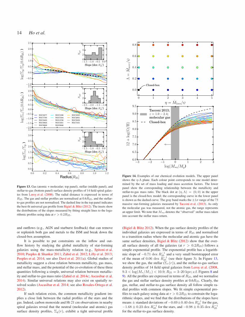
Figure 13. Gas (atomic + molecular; top panel), stellar (middle panel), and
stellar-to-gas (bottom panel) surface density profiles of 14 field spiral galax-
ies from Leroy et al. (2008). The radial distance is expressed in terms of
R25. The gas and stellar profiles are normalised at 0.6R25, and the stellar-
to-gas profiles are not normalised. The dashed line in the top panel indicates
the best-fit universal gas profile from Bigiel & Blitz (2012). The insets show
the distributions of the slopes measured by fitting straight lines to the loga-
rithmic profiles using data at r > 0.2R25.
and outflows (e.g., AGN and starburst feedback) that can remove
or replenish both gas and metals to the ISM and break down the
closed-box assumption.
It is possible to put constraints on the inflow and out-
flow history by studying the global metallicity of star-forming
galaxies using the mass-metallicity relation (e.g., Spitoni et al.
2010; Peeples & Shankar 2011; Zahid et al. 2012; Lilly et al. 2013;
Peeples et al. 2014; see also Dave et al. 2011a). Global studies of
metallicity suggest a close relation between metallicity, gas mass,
and stellar mass, and the potential of the co-evolution of these three
quantities following a simple, universal relation between metallic-
ity and stellar-to-gas mass ratio (Zahid et al. 2014c; Ascasibar et al.
2014). Similar universal relations may also exist on spatially re-
solved scales (Ascasibar et al. 2014; see also Rosales-Ortega et al.
2012).
If such relation exists, the common metallicity gradient im-
plies a close link between the radial profiles of the stars and the
gas. Indeed, carbon monoxide and HI 21 cm observations in nearby
spiral galaxies reveal that the neutral (molecular and atomic) gas
surface density profiles, Σg(r), exhibit a tight universal profile
0 1 2 3 4 5
η = Mloss/ψ
0.0
0.2
0.4
0.6
0.8
Λ=M
accr/ψ
Closed-box
−3 −2 −1 0 1 2 3
log(M∗o/Mg)
6.0
6.5
7.0
7.5
8.0
8.5
9.0
9.5
12+log(O/H)
Tacconi 2013;z = 1.0− 2.4;molecular gas
Closed-box
Figure 14. Examples of our chemical evolution models. The upper panel
shows the η-Λ plane. Each colour point corresponds to one model deter-
mined by the set of mass loading and mass accretion factors. The lower
panel show the corresponding relationship between the metallicity and
stellar-to-gas mass ratio. The black dot at (η,Λ) = (0, 0) in the upper
panel is the closed-box model; the corresponding curve in the lower panel
is shown as the dashed curve. The gray band marks the ±1σ range of the 73
massive star-forming galaxies measured by Tacconi et al. (2013). As only
the molecular gas was measured, not the atomic gas, the range represents
an upper limit. We note thatM∗o denotes the “observed” stellar mass taken
into account the stellar mass return.
(Bigiel & Blitz 2012). When the gas surface density profiles of the
individual galaxies are expressed in terms of R25 and normalised
to a transition radius where the molecular and atomic gas have the
same surface densities, Bigiel & Blitz (2012) show that the over-
all surface density of all the galaxies (at r > 0.2R25) follows a
simple exponential profile. The exponential profile has a logarith-
mic slope of −0.71 dex R−125 and a very small bootstrapped error
of the mean of 0.06 dex R−125 (see their figure 3). In Figure 13,
we show the gas, the stellar (Σ∗(r)), and the stellar-to-gas surface
density profiles of 14 field spiral galaxies from Leroy et al. (2008,
9.3 < log(M∗/M⊙) < 10.9; R25 = 3–20 kpc; c.f. Figures 8 and
9). All the profiles are expressed in terms ofR25, and we normalise
the gas and stellar surface density profiles at 0.6R25. Clearly, the
gas, stellar, and stellar-to-gas surface density all follow simple ra-
dial profiles with common slopes. We fit simple exponential pro-
files to each galaxy using data at r > 0.2R25 to constrain the loga-
rithmic slopes, and we find that the distributions of the slopes have
means ± standard deviations of −0.69±0.40 dexR−125 for the gas,
−1.68 ± 0.23 dex R−125 for the stars, and −0.98 ± 0.35 dex R−1
25
for the stellar-to-gas surface density.

Metallicity gradients in local field star-forming galaxies 15
These tight universal profiles, in particular the stellar-to-gas
mass ratio, may govern the common metallicity gradient in disk
galaxies. We use simple chemical evolution models to quantita-
tively address the relation between metallicity, and stellar-to-gas
mass ratio. The models we adopted are special cases of the more
general derivations by Recchi et al. (2008). Similar models have
been applied to global metallicities of galaxies (e.g., Spitoni et al.
2010; Dayal et al. 2013; Lilly et al. 2013; Pipino et al. 2014). The
analytical models consider, for a given volume element, metal pro-
duction by stars, stellar mass return, inflows, and outflows, under
the assumption that the gas is well-mixed and the mass return from
stars is recycled instantaneously. The inflows and outflows are de-
scribed through two critical parameters: the mass loading factor
η ≡Mloss
ψ(6)
and the mass accretion factor
Λ ≡Maccr
ψ, (7)
where Mloss and Maccr are the mass-loss and mass-gain rates, re-
spectively, and ψ is the SFR. We assume that the accreted gas is
metal-free and the outflowing gas has the same metallicity as the
ISM at the time the outflows are launched. While we make no as-
sumption on the star formation, inflow and outflow histories, we
require the mass loading and mass accretion factors to be con-
stant. We justify and discuss these assumptions in Appendix A. Un-
der these assumptions, a pair of non-negative (η,Λ) determines a
unique analytical solution for the metallicity and the stellar-to-gas
mass ratio:
Z(t) =y
Λ
1−
[
1 +
(
1 +η − Λ
1−R
)
M∗o(t)
Mg(t)
]− Λ1−R+η−Λ
,
(8)
where
η ≥ 0, Λ > 0, andη − Λ
1−R6= −1. (9)
That is, the stellar-to-gas mass ratio at any given time dictates the
metallicity at that instant. The reader is directed to Appendix A for
derivation of the models and special cases when the conditions in
Equation 9 are not met. We also show in Appendix A that in the
trivial case where there are no inflows nor outflows, i.e. η = 0 and
Λ = 0, our model is identical to the classical closed-box model
(i.e. Equation 5).
In Figure 14, we present the relationships between the metal-
licity and stellar-to-gas mass ratio (lower panel) using different sets
of (η,Λ) values (upper panel). We adopt the yield for the oxygen of
0.0031 and the returned mass fraction of 0.2, and we will discuss
the systematics of these two constants later. The classical closed-
box model, which corresponds to the origin on the η - Λ plane
(upper panel), is also shown as the dashed line in the lower panel.
In the gas rich regime, i.e. log(M∗o/Mg) ≪ −0.5, all the mod-
els coalesce as, under vast gas reservoirs, inflows and outflows do
not change the metallicity appreciably. In the gas poor regime, i.e.
log(M∗o/Mg) ≫ −0.5, for a given stellar-to-gas mass ratio the
metallicity is sensitive to the adopted mass loading and mass ac-
cretion factors. This regime can be explored with the the 14 field
spiral galaxies from Leroy et al. (2008) (0 . log(Σ∗/Σg) . 2; c.f.
Figure 13), which could place constraints on the mass loading and
mass accretion factors.
By combining the models and the measured stellar-to-gas
mass profiles of the 14 field spiral galaxies, we can predict their
metallicity gradients. The predicted metallicity gradients can be
compared with our benchmark gradient to place constraints on the
models. We calculate the predicted metallicity gradients by first
converting the stellar-to-gas mass ratios to metallicities for each
radial bins, and we fit linear profiles to data at r > 0.2R25 in each
galaxies to derive the predicted metallicity gradients. In Figure 15,
we show the distributions of the predicted metallicity gradients us-
ing a grid of (η,Λ). In the top and middle panel of Figure 16,
we compare the means and standard deviations of the predicted
metallicity gradients to those from our benchmark gradient. In the
bottom panel, we perform one-sample Kolmogorov-Smirnov tests
to compare the distributions of the predicted metallicity gradients
with the benchmark gradient that has a Gaussian distribution of
−0.39± 0.18 dex R−125 (mean ± standard deviation; Figure 11).
Figure 15 qualitatively demonstrates that small η and Λ val-
ues (panels toward the lower left corner) are preferred because
the predicted distributions are similar to the benchmark gradient.
Large η and Λ values tend to overproduce flatter metallicity gra-
dients, effectively shifting the means of the distributions towards
zero and reducing the widths of the distributions. This behaviour
can be trivially understood with the bottom panel of Figure 14
where the models with large η and Λ values flatten at high stellar-
to-gas mass ratios, yielding the same metallicities across the disks,
i.e. flat metallicity gradients. We quantitatively address the allowed
η and Λ values in Figure 16 by investigating the differences of
the means (upper panel), those of the standard deviations (middle
panel), and the probabilities of reproducing the benchmark gradient
through the Kolmogorov-Smirnov test (bottom panel). We find that
for 0 . Λ . 0.3 and 0 . η . 2.5, the Kolmogorov-Smirnov tests
yield good probabilities (& 20%) for the distributions of the pre-
dicted metallicity gradients to be drawn from the benchmark gra-
dient. Within the same ranges, the differences between the mean
of the benchmark gradient and those of the predicted gradients are
within about 20%, and the differences between the standard devi-
ations are also within about 20%. Interestingly, the differences of
the means, and those of the standard deviations both show that the
closed-box model is the best model, but the Kolmogorov-Smirnov
tests suggest that low (but non-zero) mass loading and mass accre-
tion factors are more preferred. While the precise values of η and
Λ probably cannot be determined from the 14 galaxies alone (due
to low number statistics) and are likely to vary from system to sys-
tem, closed-box and virtually closed-box are the models that can
successfully reproduce the observed benchmark gradient.
The success of reproducing the benchmark gradient with our
simple models, however, do not imply that all galaxies evolve as
closed-box or virtually closed-box throughout their lifetime. Nor
do our results support the idea that galaxies always have con-
stant mass loading and mass accretion factors, either on global
or spatially resolved scales. Observations of high-redshift galax-
ies (z > 1) have provided evidences that galaxies in the early
Universe undergo many, perhaps intermittent, accretion events,
immense star formation and outflows (e.g., Tacconi et al. 2010,
2013; Weiner et al. 2009; Steidel et al. 2010; Genzel et al. 2011;
Newman et al. 2012; Genzel et al. 2014). Similar outflows, in par-
ticular the starburst-driven winds, are found to be ubiquitously in
galaxies at lower redshifts with high enough star-formation sur-
face density (Heckman 2002), with the wind velocities showing
indication of correlating with both the SFR and host galaxy mass
(Rupke et al. 2005a,b; Veilleux et al. 2005; Chen et al. 2010). En-
ergy and mass return from both the stars and AGNs (i.e. “feed-
back”) are indispensable for numerical simulations to reproduce
many observed properties of galaxies, such as the stellar mass
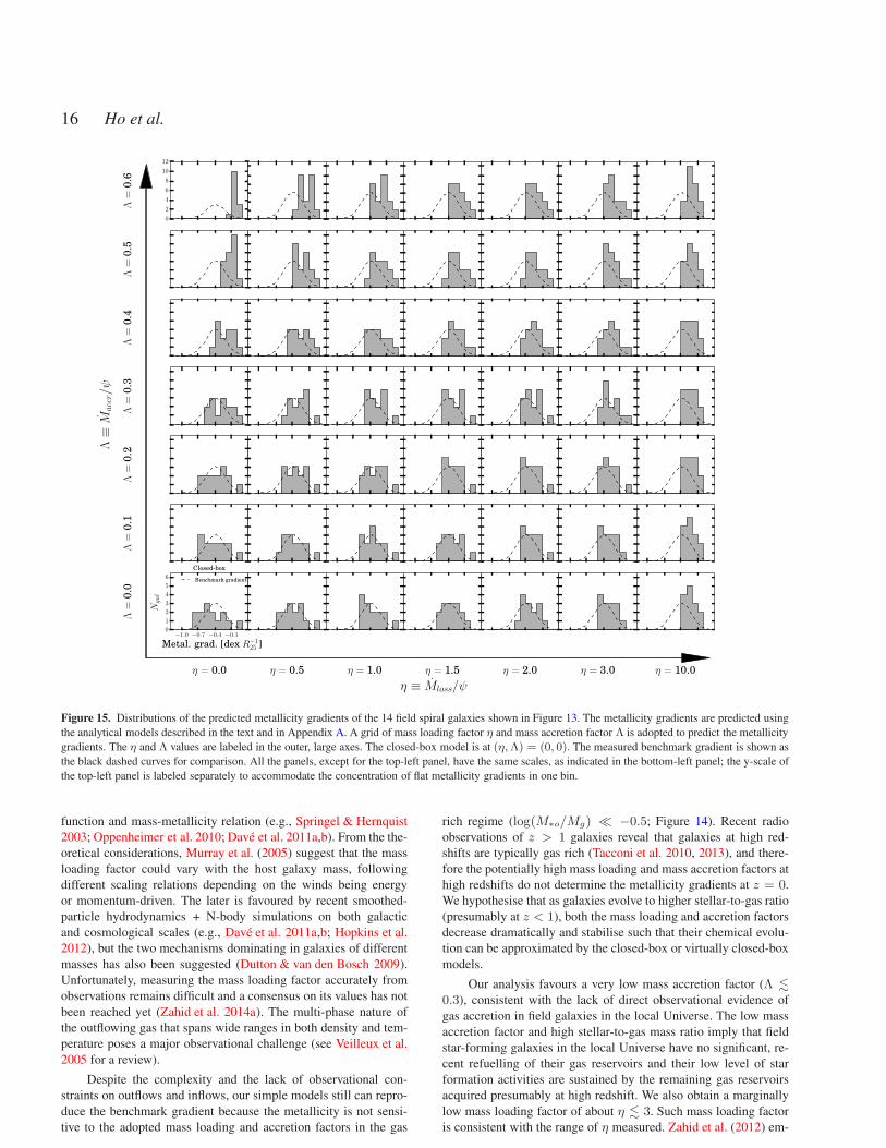
16 Ho et al.
0
2
4
6
8
10
12
−1.0 −0.7 −0.4 −0.1
Metal. grad. [dex R−1
25]
0
1
2
3
4
5
6
Ngal
Closed-box
Benchmark gradient
η ≡ Mloss/ψ
Λ≡M
accr/ψ
η = 0.0 η = 0.5 η = 1.0 η = 1.5 η = 2.0 η = 3.0 η = 10.0
Λ=
0.0
Λ=
0.1
Λ=
0.2
Λ=
0.3
Λ=
0.4
Λ=
0.5
Λ=
0.6
Figure 15. Distributions of the predicted metallicity gradients of the 14 field spiral galaxies shown in Figure 13. The metallicity gradients are predicted using
the analytical models described in the text and in Appendix A. A grid of mass loading factor η and mass accretion factor Λ is adopted to predict the metallicity
gradients. The η and Λ values are labeled in the outer, large axes. The closed-box model is at (η,Λ) = (0, 0). The measured benchmark gradient is shown as
the black dashed curves for comparison. All the panels, except for the top-left panel, have the same scales, as indicated in the bottom-left panel; the y-scale of
the top-left panel is labeled separately to accommodate the concentration of flat metallicity gradients in one bin.
function and mass-metallicity relation (e.g., Springel & Hernquist
2003; Oppenheimer et al. 2010; Dave et al. 2011a,b). From the the-
oretical considerations, Murray et al. (2005) suggest that the mass
loading factor could vary with the host galaxy mass, following
different scaling relations depending on the winds being energy
or momentum-driven. The later is favoured by recent smoothed-
particle hydrodynamics + N-body simulations on both galactic
and cosmological scales (e.g., Dave et al. 2011a,b; Hopkins et al.
2012), but the two mechanisms dominating in galaxies of different
masses has also been suggested (Dutton & van den Bosch 2009).
Unfortunately, measuring the mass loading factor accurately from
observations remains difficult and a consensus on its values has not
been reached yet (Zahid et al. 2014a). The multi-phase nature of
the outflowing gas that spans wide ranges in both density and tem-
perature poses a major observational challenge (see Veilleux et al.
2005 for a review).
Despite the complexity and the lack of observational con-
straints on outflows and inflows, our simple models still can repro-
duce the benchmark gradient because the metallicity is not sensi-
tive to the adopted mass loading and accretion factors in the gas
rich regime (log(M∗o/Mg) ≪ −0.5; Figure 14). Recent radio
observations of z > 1 galaxies reveal that galaxies at high red-
shifts are typically gas rich (Tacconi et al. 2010, 2013), and there-
fore the potentially high mass loading and mass accretion factors at
high redshifts do not determine the metallicity gradients at z = 0.
We hypothesise that as galaxies evolve to higher stellar-to-gas ratio
(presumably at z < 1), both the mass loading and accretion factors
decrease dramatically and stabilise such that their chemical evolu-
tion can be approximated by the closed-box or virtually closed-box
models.
Our analysis favours a very low mass accretion factor (Λ .
0.3), consistent with the lack of direct observational evidence of
gas accretion in field galaxies in the local Universe. The low mass
accretion factor and high stellar-to-gas mass ratio imply that field
star-forming galaxies in the local Universe have no significant, re-
cent refuelling of their gas reservoirs and their low level of star
formation activities are sustained by the remaining gas reservoirs
acquired presumably at high redshift. We also obtain a marginally
low mass loading factor of about η . 3. Such mass loading factor
is consistent with the range of η measured. Zahid et al. (2012) em-
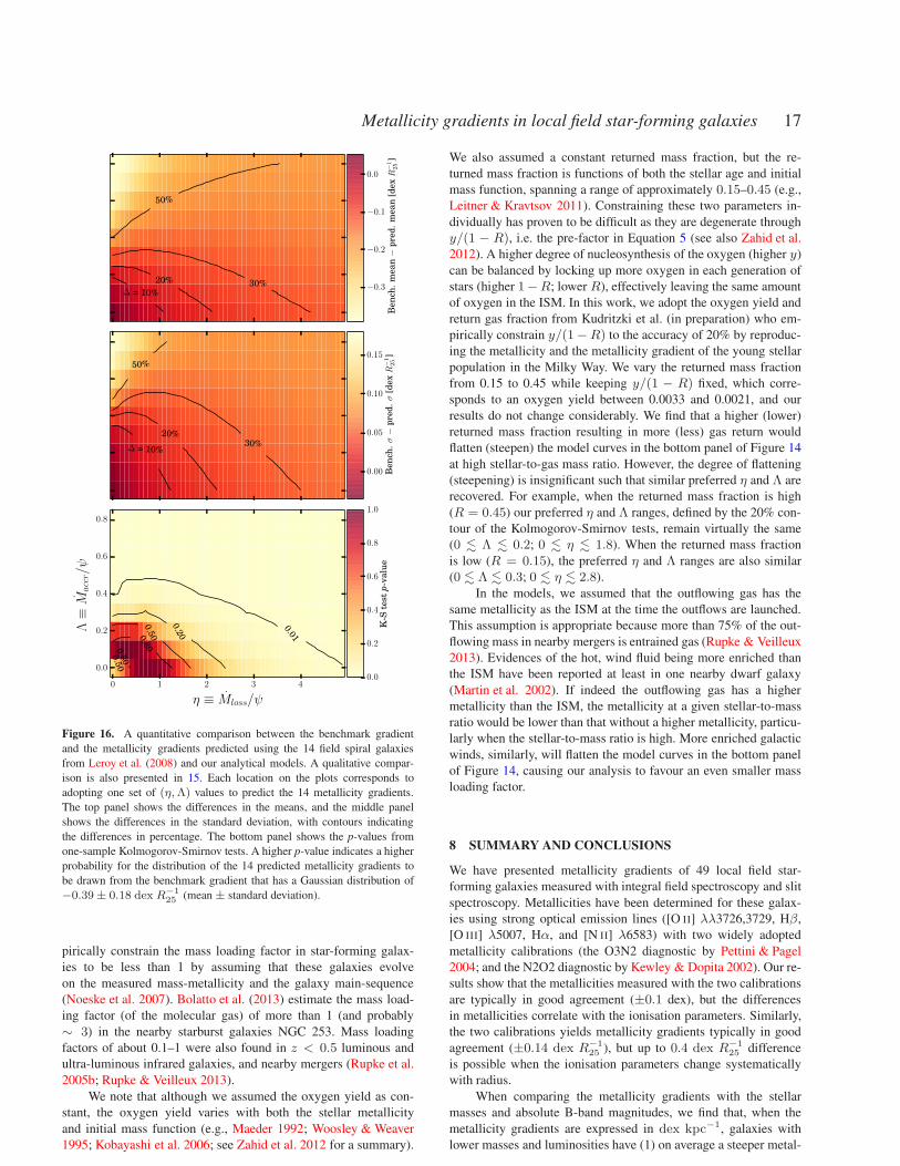
Metallicity gradients in local field star-forming galaxies 17
∆ = 10%
20% 30%
50%
∆ = 10%
20%30%
50%
0 1 2 3 4
η ≡ Mloss/ψ
0.0
0.2
0.4
0.6
0.8
Λ≡M
accr/ψ
0.01
0.2
0
0.5
0
0.5
0
0.8
0
0.8
0
−0.3
−0.2
−0.1
0.0
Ben
ch.
mean−
pre
d.
mean
[dexR
−1
25
]
0.00
0.05
0.10
0.15
Ben
ch.σ−
pre
d.σ
[dexR
−1
25
]
0.0
0.2
0.4
0.6
0.8
1.0
K-S
test
p-v
alu
e
Figure 16. A quantitative comparison between the benchmark gradient
and the metallicity gradients predicted using the 14 field spiral galaxies
from Leroy et al. (2008) and our analytical models. A qualitative compar-
ison is also presented in 15. Each location on the plots corresponds to
adopting one set of (η,Λ) values to predict the 14 metallicity gradients.
The top panel shows the differences in the means, and the middle panel
shows the differences in the standard deviation, with contours indicating
the differences in percentage. The bottom panel shows the p-values from
one-sample Kolmogorov-Smirnov tests. A higher p-value indicates a higher
probability for the distribution of the 14 predicted metallicity gradients to
be drawn from the benchmark gradient that has a Gaussian distribution of
−0.39± 0.18 dex R−125 (mean ± standard deviation).
pirically constrain the mass loading factor in star-forming galax-
ies to be less than 1 by assuming that these galaxies evolve
on the measured mass-metallicity and the galaxy main-sequence
(Noeske et al. 2007). Bolatto et al. (2013) estimate the mass load-
ing factor (of the molecular gas) of more than 1 (and probably
∼ 3) in the nearby starburst galaxies NGC 253. Mass loading
factors of about 0.1–1 were also found in z < 0.5 luminous and
ultra-luminous infrared galaxies, and nearby mergers (Rupke et al.
2005b; Rupke & Veilleux 2013).
We note that although we assumed the oxygen yield as con-
stant, the oxygen yield varies with both the stellar metallicity
and initial mass function (e.g., Maeder 1992; Woosley & Weaver
1995; Kobayashi et al. 2006; see Zahid et al. 2012 for a summary).
We also assumed a constant returned mass fraction, but the re-
turned mass fraction is functions of both the stellar age and initial
mass function, spanning a range of approximately 0.15–0.45 (e.g.,
Leitner & Kravtsov 2011). Constraining these two parameters in-
dividually has proven to be difficult as they are degenerate through
y/(1 − R), i.e. the pre-factor in Equation 5 (see also Zahid et al.
2012). A higher degree of nucleosynthesis of the oxygen (higher y)
can be balanced by locking up more oxygen in each generation of
stars (higher 1−R; lower R), effectively leaving the same amount
of oxygen in the ISM. In this work, we adopt the oxygen yield and
return gas fraction from Kudritzki et al. (in preparation) who em-
pirically constrain y/(1−R) to the accuracy of 20% by reproduc-
ing the metallicity and the metallicity gradient of the young stellar
population in the Milky Way. We vary the returned mass fraction
from 0.15 to 0.45 while keeping y/(1 − R) fixed, which corre-
sponds to an oxygen yield between 0.0033 and 0.0021, and our
results do not change considerably. We find that a higher (lower)
returned mass fraction resulting in more (less) gas return would
flatten (steepen) the model curves in the bottom panel of Figure 14
at high stellar-to-gas mass ratio. However, the degree of flattening
(steepening) is insignificant such that similar preferred η and Λ are
recovered. For example, when the returned mass fraction is high
(R = 0.45) our preferred η and Λ ranges, defined by the 20% con-
tour of the Kolmogorov-Smirnov tests, remain virtually the same
(0 . Λ . 0.2; 0 . η . 1.8). When the returned mass fraction
is low (R = 0.15), the preferred η and Λ ranges are also similar
(0 . Λ . 0.3; 0 . η . 2.8).
In the models, we assumed that the outflowing gas has the
same metallicity as the ISM at the time the outflows are launched.
This assumption is appropriate because more than 75% of the out-
flowing mass in nearby mergers is entrained gas (Rupke & Veilleux
2013). Evidences of the hot, wind fluid being more enriched than
the ISM have been reported at least in one nearby dwarf galaxy
(Martin et al. 2002). If indeed the outflowing gas has a higher
metallicity than the ISM, the metallicity at a given stellar-to-mass
ratio would be lower than that without a higher metallicity, particu-
larly when the stellar-to-mass ratio is high. More enriched galactic
winds, similarly, will flatten the model curves in the bottom panel
of Figure 14, causing our analysis to favour an even smaller mass
loading factor.
8 SUMMARY AND CONCLUSIONS
We have presented metallicity gradients of 49 local field star-
forming galaxies measured with integral field spectroscopy and slit
spectroscopy. Metallicities have been determined for these galax-
ies using strong optical emission lines ([O II] λλ3726,3729, Hβ,
[O III] λ5007, Hα, and [N II] λ6583) with two widely adopted
metallicity calibrations (the O3N2 diagnostic by Pettini & Pagel
2004; and the N2O2 diagnostic by Kewley & Dopita 2002). Our re-
sults show that the metallicities measured with the two calibrations
are typically in good agreement (±0.1 dex), but the differences
in metallicities correlate with the ionisation parameters. Similarly,
the two calibrations yields metallicity gradients typically in good
agreement (±0.14 dex R−125 ), but up to 0.4 dex R−1
25 difference
is possible when the ionisation parameters change systematically
with radius.
When comparing the metallicity gradients with the stellar
masses and absolute B-band magnitudes, we find that, when the
metallicity gradients are expressed in dex kpc−1, galaxies with
lower masses and luminosities have (1) on average a steeper metal-
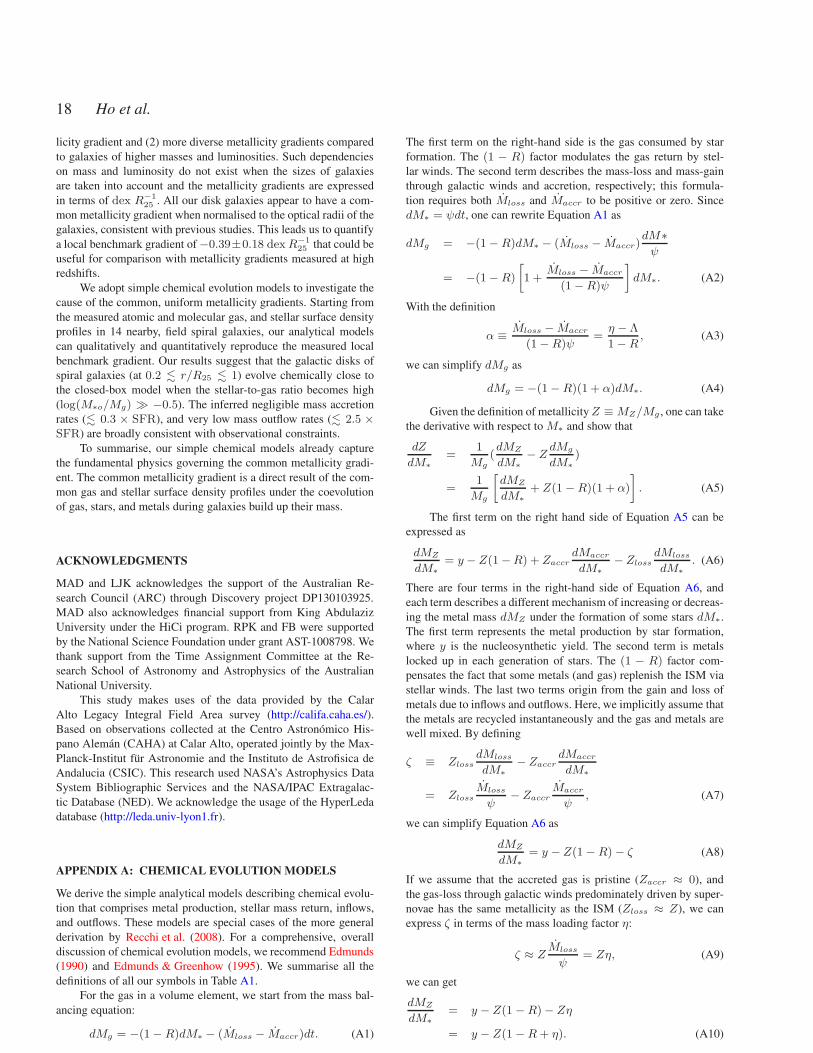
18 Ho et al.
licity gradient and (2) more diverse metallicity gradients compared
to galaxies of higher masses and luminosities. Such dependencies
on mass and luminosity do not exist when the sizes of galaxies
are taken into account and the metallicity gradients are expressed
in terms of dex R−125 . All our disk galaxies appear to have a com-
mon metallicity gradient when normalised to the optical radii of the
galaxies, consistent with previous studies. This leads us to quantify
a local benchmark gradient of −0.39±0.18 dexR−125 that could be
useful for comparison with metallicity gradients measured at high
redshifts.
We adopt simple chemical evolution models to investigate the
cause of the common, uniform metallicity gradients. Starting from
the measured atomic and molecular gas, and stellar surface density
profiles in 14 nearby, field spiral galaxies, our analytical models
can qualitatively and quantitatively reproduce the measured local
benchmark gradient. Our results suggest that the galactic disks of
spiral galaxies (at 0.2 . r/R25 . 1) evolve chemically close to
the closed-box model when the stellar-to-gas ratio becomes high
(log(M∗o/Mg) ≫ −0.5). The inferred negligible mass accretion
rates (. 0.3 × SFR), and very low mass outflow rates (. 2.5 ×SFR) are broadly consistent with observational constraints.
To summarise, our simple chemical models already capture
the fundamental physics governing the common metallicity gradi-
ent. The common metallicity gradient is a direct result of the com-
mon gas and stellar surface density profiles under the coevolution
of gas, stars, and metals during galaxies build up their mass.
ACKNOWLEDGMENTS
MAD and LJK acknowledges the support of the Australian Re-
search Council (ARC) through Discovery project DP130103925.
MAD also acknowledges financial support from King Abdulaziz
University under the HiCi program. RPK and FB were supported
by the National Science Foundation under grant AST-1008798. We
thank support from the Time Assignment Committee at the Re-
search School of Astronomy and Astrophysics of the Australian
National University.
This study makes uses of the data provided by the Calar
Alto Legacy Integral Field Area survey (http://califa.caha.es/).
Based on observations collected at the Centro Astronomico His-
pano Aleman (CAHA) at Calar Alto, operated jointly by the Max-
Planck-Institut fur Astronomie and the Instituto de Astrofisica de
Andalucia (CSIC). This research used NASA’s Astrophysics Data
System Bibliographic Services and the NASA/IPAC Extragalac-
tic Database (NED). We acknowledge the usage of the HyperLeda
database (http://leda.univ-lyon1.fr).
APPENDIX A: CHEMICAL EVOLUTION MODELS
We derive the simple analytical models describing chemical evolu-
tion that comprises metal production, stellar mass return, inflows,
and outflows. These models are special cases of the more general
derivation by Recchi et al. (2008). For a comprehensive, overall
discussion of chemical evolution models, we recommend Edmunds
(1990) and Edmunds & Greenhow (1995). We summarise all the
definitions of all our symbols in Table A1.
For the gas in a volume element, we start from the mass bal-
ancing equation:
dMg = −(1−R)dM∗ − (Mloss − Maccr)dt. (A1)
The first term on the right-hand side is the gas consumed by star
formation. The (1 − R) factor modulates the gas return by stel-
lar winds. The second term describes the mass-loss and mass-gain
through galactic winds and accretion, respectively; this formula-
tion requires both Mloss and Maccr to be positive or zero. Since
dM∗ = ψdt, one can rewrite Equation A1 as
dMg = −(1−R)dM∗ − (Mloss − Maccr)dM∗
ψ
= −(1−R)
[
1 +Mloss − Maccr
(1−R)ψ
]
dM∗. (A2)
With the definition
α ≡Mloss − Maccr
(1−R)ψ=η − Λ
1−R, (A3)
we can simplify dMg as
dMg = −(1−R)(1 + α)dM∗. (A4)
Given the definition of metallicityZ ≡MZ/Mg , one can take
the derivative with respect to M∗ and show that
dZ
dM∗
=1
Mg(dMZ
dM∗
− ZdMg
dM∗
)
=1
Mg
[
dMZ
dM∗
+ Z(1−R)(1 + α)
]
. (A5)
The first term on the right hand side of Equation A5 can be
expressed as
dMZ
dM∗
= y − Z(1−R) + ZaccrdMaccr
dM∗
−ZlossdMloss
dM∗
. (A6)
There are four terms in the right-hand side of Equation A6, and
each term describes a different mechanism of increasing or decreas-
ing the metal mass dMZ under the formation of some stars dM∗.
The first term represents the metal production by star formation,
where y is the nucleosynthetic yield. The second term is metals
locked up in each generation of stars. The (1 − R) factor com-
pensates the fact that some metals (and gas) replenish the ISM via
stellar winds. The last two terms origin from the gain and loss of
metals due to inflows and outflows. Here, we implicitly assume that
the metals are recycled instantaneously and the gas and metals are
well mixed. By defining
ζ ≡ ZlossdMloss
dM∗
− ZaccrdMaccr
dM∗
= ZlossMloss
ψ− Zaccr
Maccr
ψ, (A7)
we can simplify Equation A6 as
dMZ
dM∗
= y − Z(1−R)− ζ (A8)
If we assume that the accreted gas is pristine (Zaccr ≈ 0), and
the gas-loss through galactic winds predominately driven by super-
novae has the same metallicity as the ISM (Zloss ≈ Z), we can
express ζ in terms of the mass loading factor η:
ζ ≈ ZMloss
ψ= Zη, (A9)
we can get
dMZ
dM∗
= y − Z(1−R)− Zη
= y − Z(1−R+ η). (A10)

Metallicity gradients in local field star-forming galaxies 19
Table A1. Key for Symbols
Symbol Definition
Mg Hydrogen gas mass
M∗ Stellar mass (without considering mass return)
ψ ≡ dM∗/dt; SFR
R Returned mass fraction; fraction of stellar mass which goes back to ISM through stellar winds
M∗o ≡ (1− R)M∗; observed stellar mass taking into account mass return
MZ Metal mass
Z ≡ MZ/Mg ; ISM metallicity. Note that Z is the mass ratio, as opposed to the number ratio in 12 + log(O/H)y Nucleosynthetic yield; dZ = ydM∗
Mloss Rate of mass-loss of gas through galactic winds
Maccr Rate of mass-gain of gas through accretion
dM∗ ≡ ψdt; stellar mass formed through star formation
dMaccr ≡ Maccrdt
dMloss ≡ Mlossdt
η ≡ Mloss/ψ ≥ 0; mass loading factor; mass-loss per star formed
Λ ≡ Maccr/ψ ≥ 0 ; mass accretion factor; mass-gain per star formed
Zaccr Metallicity of the accreted gas
Zloss Metallicity of the outflowing gas
The assumption that Zloss ≈ Z is valid if most of the out-
flowing gas is entrained ISM close to the energy sources (e.g. su-
pernovae). Indeed, more than 75% of the outflowing gas is esti-
mated to be entrained gas in nearby mergers (Rupke & Veilleux
2013). The metallicity of the hot, wind fluid is found to be higher
than the ISM metallicity in one nearby dwarf galaxy NGC 1569
(Martin et al. 2002), perhaps indicating that the hot materials can
survive the gravitational potential better than the cold entrained
gas, but constraints on the metallicity of the outflowing gas remain
scarce because X-ray observations are often required. The reader is
directed to Dalcanton (2007) for models where Zaccr and Zloss are
arbitrary.
It is worth pointing out that by definition η and Λ must be
positive or zero
η ≥ 0 and Λ ≥ 0, (A11)
because of the ways Mloss and Maccr were defined. However, αdefined in Eqaution A3 can be both positive (outflow dominates),
negative (inflow dominates), or zero (balance between inflows and
outflows).
To solve the relation between Z, M∗ and Mg , we further as-
sume that R, y, η, and Λ (and therefore α) are all constants. We
discuss the changes in our results when adopting different R and
y in Section 7. Assuming constant mass-loading and mass accre-
tion factors allows the derivation to remain simple and analytic,
and the assumptions carry significant physical meanings. The con-
stant mass-loading factor is postulated because the energy driving
the outflowing mass is from star formation, and η simply reflects
the efficiency in transferring energy from star formation to the out-
flowing gas. Similarly, because the inflowing gas supplies the reser-
voir for star formation, the constant mass accretion factor can be re-
alised as the efficiency of collapsing the gas into stars. We explore
different η and Λ values in Section 7 to understand the possible
impact of them not being constant over time. Recchi et al. (2008)
explore non-constant Λ by assuming exponential inflows and a lin-
ear Schmidt law. They conclude that constant Λ is a reasonable ap-
proximation of the late evolution of a galaxy provided that the infall
timescale is of the same order of magnitude of the star formation
timescale.
With the relation between MZ and M∗ in Equation A10, one
can readily rewrite Equation A5 as
dZ
dM∗
=1
Mg[y − Z(1−R + η) + Z(1−R)(1 + α)]
=1
Mg(y − ZΛ). (A12)
Given the relation between dM∗ and dMg in Equation A4, we find
(1−R)(1 + α)
ZΛ− ydZ =
1
MgdMg, (A13)
and therefore
(1−R)(1 + α)
Λln(ZΛ− y)|
Z(t)Z=0= lnMg|
Mg(t)
Mg=Mg(0). (A14)
We note that this solution is only valid for α different from −1. We
will discuss the case α = −1 separately below.
To proceed, one needs to know the relation between Mg(t)and Mg(0). This can be done by integrating Equation A4
Mg |Mg(t)
Mg=Mg(0)= −(1−R)(1 + α)M∗|
M∗(t)M∗=0;
therefore
Mg(0) =Mg(t) + (1−R)(1 + α)M∗(t), (A15)
Finally, from Equation A14 and Equation A15, we arrive at
Z(t) =y
Λ
1−
[
1 + (1−R)(1 + α)M∗(t)
Mg(t)
]− Λ(1−R)(1+α)
=y
Λ
1−
[
1 + (1 + α)M∗o(t)
Mg(t)
]−Λ
(1−R)(1+α)
,
(A16)
or equivalently with the definition of α in Equation A3:
Z(t) =y
Λ
1−
[
1 +
(
1 +η − Λ
1−R
)
M∗o(t)
Mg(t)
]−Λ
1−R+η−Λ
,
where η ≥ 0, Λ > 0, andη − Λ
1−R6= −1. (A17)
Note that the solutions, Equations A16 and A17, have an infinite

20 Ho et al.
exponent for the case α = −1, which was excluded when we de-
rived these solutions. However, the case α = −1 can be easily
addressed. First, we note that from Equation A4 we obtain in this
case Mg(t) = const. and that Λ becomes
Λ = (1−R) + η (A18)
WithMg(t) = const. we can then directly integrate Equation A12
and obtain
Z(t) =y
Λ(1− e
−ΛM∗(t)Mg(t) ). (A19)
Or equivalently by replacing Λ through Equation A18, we arrive at
Z(t) =
(
y
1−R
)
(
1
1 + η1−R
)
[
1− e−(1+ η
1−R)M∗o(t)Mg(t)
]
,
when η = Λ− (1−R). (A20)
In the extreme case where there is only outflows and virtually
no inflows, i.e. η 6= 0 and Λ = 0, Equations A16 and A17 are no
longer valid as both the numerator and denominator approach zero.
One can repeat the derivation from Equation A12 with Λ = 0 and
trivially show that
Z(t) =
(
y
1−R
)
(
1
1 + η1−R
)
ln
[
1 +
(
1 +η
1−R
)
M∗o(t)
Mg(t)
]
,
when η 6= 0 and Λ = 0. (A21)
In another extreme where there is only inflows but no outflows
(Λ 6= 0 and η = 0), Equations A16 and A17 are valid and the
reader is also directed to the similar models by Koppen & Edmunds
(1999).
In the special case where there are no inflows nor outflows
Equation A21 becomes:
Z(t) =y
1−Rln
[
1 +M∗o(t)
Mg(t)
]
, when η = 0 and Λ = 0.
(A22)
Equation A22, same as Equation 5, is the classical closed-box so-
lution (Searle & Sargent 1972; Pagel & Patchett 1975).
APPENDIX B: METALLICITY GRADIENTS AND
IONISATION PARAMETERS OF INDIVIDUAL GALAXIES
Figures B1 and B2 show the metallicity gradients and ionisation pa-
rameters for the rest of the CALIFA and S12 samples, respectively.
These are in addition to the four galaxies presented in Figures 4 and
5. Figure B3 show those for the WiFeS galaxies.
REFERENCES
Abazajian K. N. et al., 2009, ApJS, 182, 543
Allen J. T. et al., 2014, ArXiv e-prints
Ascasibar Y., Gavilan M., Pinto N., Casado J., Rosales F., Dıaz
A. I., 2014, ArXiv e-prints
Baldwin J. A., Phillips M. M., Terlevich R., 1981, PASP, 93, 5
Bigiel F., Blitz L., 2012, ApJ, 756, 183
Blanc G. A., Heiderman A., Gebhardt K., Evans II N. J., Adams
J., 2009, ApJ, 704, 842
Bland-Hawthorn J., 2014, ArXiv e-prints
Bolatto A. D. et al., 2013, Nature, 499, 450
Bothun G. D., Romanishin W., Strom S. E., Strom K. M., 1984,
AJ, 89, 1300
Bresolin F., Kennicutt R. C., Ryan-Weber E., 2012, ApJ, 750, 122
Brooks A. M., Governato F., Booth C. M., Willman B., Gardner
J. P., Wadsley J., Stinson G., Quinn T., 2007, ApJ, 655, L17
Bruzual G., Charlot S., 2003, MNRAS, 344, 1000
Bryant J. J. et al., 2014, ArXiv e-prints
Calura F., Pipino A., Chiappini C., Matteucci F., Maiolino R.,
2009, A&A, 504, 373
Calzetti D., Armus L., Bohlin R. C., Kinney A. L., Koornneef J.,
Storchi-Bergmann T., 2000, ApJ, 533, 682
Cappellari M., Emsellem E., 2004, PASP, 116, 138
Cardelli J. A., Clayton G. C., Mathis J. S., 1989, ApJ, 345, 245
Chabrier G., 2003, PASP, 115, 763
Chen Y. M., Tremonti C. A., Heckman T. M., Kauffmann G.,
Weiner B. J., Brinchmann J., Wang J., 2010, AJ, 140, 445
Chiappini C., Matteucci F., Gratton R., 1997, ApJ, 477, 765
Chiappini C., Matteucci F., Romano D., 2001, ApJ, 554, 1044
Childress M. J., Vogt F. P. A., Nielsen J., Sharp R. G., 2014,
Ap&SS, 349, 617
Cid Fernandes R. et al., 2014, A&A, 561, A130
Conroy C., Gunn J. E., White M., 2009, ApJ, 699, 486
Cresci G., Mannucci F., Maiolino R., Marconi A., Gnerucci A.,
Magrini L., 2010, Nature, 467, 811
Croom S. M. et al., 2012, MNRAS, 421, 872
Dalcanton J. J., 2007, ApJ, 658, 941
Dalcanton J. J., Yoachim P., Bernstein R. A., 2004, ApJ, 608, 189
Dave R., Finlator K., Oppenheimer B. D., 2011a, MNRAS, 416,
1354
Dave R., Oppenheimer B. D., Finlator K., 2011b, MNRAS, 415,
11
Dayal P., Ferrara A., Dunlop J. S., 2013, MNRAS, 430, 2891
Dopita M., Hart J., McGregor P., Oates P., Bloxham G., Jones D.,
2007, Ap&SS, 310, 255
Dopita M. et al., 2010, Ap&SS, 327, 245
Dopita M. A., Rich J., Vogt F. P. A., Kewley L. J., Ho I. T., Basurah
H. M., Ali A., Amer M. A., 2014, Ap&SS, 350, 741
Drory N., Bender R., Hopp U., 2004, ApJ, 616, L103
Dutton A. A., van den Bosch F. C., 2009, MNRAS, 396, 141
Edmunds M. G., 1990, MNRAS, 246, 678
Edmunds M. G., Greenhow R. M., 1995, MNRAS, 272, 241
Erb D. K., Shapley A. E., Pettini M., Steidel C. C., Reddy N. A.,
Adelberger K. L., 2006, ApJ, 644, 813
Few C. G., Gibson B. K., Courty S., Michel-Dansac L., Brook
C. B., Stinson G. S., 2012, A&A, 547, A63
Freeman K. C., 1970, ApJ, 160, 811
Fu J., Hou J. L., Yin J., Chang R. X., 2009, ApJ, 696, 668
Garnett D. R., 2002, ApJ, 581, 1019
Garnett D. R., Shields G. A., Skillman E. D., Sagan S. P., Dufour
R. J., 1997, ApJ, 489, 63
Genzel R. et al., 2011, ApJ, 733, 101
Genzel R. et al., 2014, ArXiv e-prints
Gonzalez Delgado R. M., Cervino M., Martins L. P., Leitherer C.,
Hauschildt P. H., 2005, MNRAS, 357, 945
Haffner L. M. et al., 2009, Reviews of Modern Physics, 81, 969
Heckman T. M., 2002, in J.S. Mulchaey, J.T. Stocke, eds, Extra-
galactic Gas at Low Redshift. Astronomical Society of the Pa-
cific Conference Series, Vol. 254, p. 292
Henry R. B. C., Edmunds M. G., Koppen J., 2000, ApJ, 541, 660
Ho I. T. et al., 2014, MNRAS, 444, 3894
Hopkins P. F., Quataert E., Murray N., 2012, MNRAS, 421, 3522

Metallicity gradients in local field star-forming galaxies 21
0.0 0.2 0.4 0.6 0.8 1.0 1.2 1.4deproj. radius[R25]
8.0
8.5
9.0
9.5
12+
log(
O/H
) O
3N2
0 2 4 6 8deproj. radius [kpc]
CALIFA:IC0776
0.0 0.2 0.4 0.6 0.8 1.0 1.2 1.4deproj. radius [R25]
8.0
8.5
9.0
9.5
12+
log(
O/H
) N
2O2
0 2 4 6 8deproj. radius [kpc]
0.0 0.2 0.4 0.6 0.8 1.0 1.2 1.4deproj. radius [R25
7.07.27.47.67.88.08.2
log(
q) [c
m/s
]
0 2 4 6 8deproj. radius [kpc]
0.0 0.2 0.4 0.6 0.8 1.0 1.2 1.4deproj. radius[R25]
8.0
8.5
9.0
9.5
12+
log(
O/H
) O
3N2
0 5 10 15deproj. radius [kpc]
CALIFA:IC1256
0.0 0.2 0.4 0.6 0.8 1.0 1.2 1.4deproj. radius [R25]
8.0
8.5
9.0
9.512
+lo
g(O
/H)
N2O
2
0 5 10 15deproj. radius [kpc]
0.0 0.2 0.4 0.6 0.8 1.0 1.2 1.4deproj. radius [R25
7.07.27.47.67.88.08.2
log(
q) [c
m/s
]
0 5 10 15deproj. radius [kpc]
0.0 0.2 0.4 0.6 0.8 1.0 1.2 1.4deproj. radius[R25]
8.0
8.5
9.0
9.5
12+
log(
O/H
) O
3N2
0 10 20 30 40deproj. radius [kpc]
CALIFA:NGC0036
0.0 0.2 0.4 0.6 0.8 1.0 1.2 1.4deproj. radius [R25]
8.0
8.5
9.0
9.5
12+
log(
O/H
) N
2O2
0 10 20 30 40deproj. radius [kpc]
0.0 0.2 0.4 0.6 0.8 1.0 1.2 1.4deproj. radius [R25
7.07.27.47.67.88.08.2
log(
q) [c
m/s
]
0 10 20 30 40deproj. radius [kpc]
0.0 0.2 0.4 0.6 0.8 1.0 1.2 1.4deproj. radius[R25]
8.0
8.5
9.0
9.5
12+
log(
O/H
) O
3N2
0 5 10 15 20 25deproj. radius [kpc]
CALIFA:NGC0477
0.0 0.2 0.4 0.6 0.8 1.0 1.2 1.4deproj. radius [R25]
8.0
8.5
9.0
9.5
12+
log(
O/H
) N
2O2
0 5 10 15 20 25deproj. radius [kpc]
0.0 0.2 0.4 0.6 0.8 1.0 1.2 1.4deproj. radius [R25
7.07.27.47.67.88.08.2
log(
q) [c
m/s
]
0 5 10 15 20 25deproj. radius [kpc]
0.0 0.2 0.4 0.6 0.8 1.0 1.2 1.4deproj. radius[R25]
8.0
8.5
9.0
9.5
12+
log(
O/H
) O
3N2
0 5 10 15 20 25deproj. radius [kpc]
CALIFA:NGC2916
0.0 0.2 0.4 0.6 0.8 1.0 1.2 1.4deproj. radius [R25]
8.0
8.5
9.0
9.5
12+
log(
O/H
) N
2O2
0 5 10 15 20 25deproj. radius [kpc]
0.0 0.2 0.4 0.6 0.8 1.0 1.2 1.4deproj. radius [R25
7.07.27.47.67.88.08.2
log(
q) [c
m/s
]
0 5 10 15 20 25deproj. radius [kpc]
0.0 0.2 0.4 0.6 0.8 1.0 1.2 1.4deproj. radius[R25]
8.0
8.5
9.0
9.5
12+
log(
O/H
) O
3N2
0 2 4 6 8deproj. radius [kpc]
CALIFA:NGC4470
0.0 0.2 0.4 0.6 0.8 1.0 1.2 1.4deproj. radius [R25]
8.0
8.5
9.0
9.5
12+
log(
O/H
) N
2O2
0 2 4 6 8deproj. radius [kpc]
0.0 0.2 0.4 0.6 0.8 1.0 1.2 1.4deproj. radius [R25
7.07.27.47.67.88.08.2
log(
q) [c
m/s
]
0 2 4 6 8deproj. radius [kpc]
0.0 0.2 0.4 0.6 0.8 1.0 1.2 1.4deproj. radius[R25]
8.0
8.5
9.0
9.5
12+
log(
O/H
) O
3N2
0 5 10 15 20deproj. radius [kpc]
CALIFA:NGC5000
0.0 0.2 0.4 0.6 0.8 1.0 1.2 1.4deproj. radius [R25]
8.0
8.5
9.0
9.5
12+
log(
O/H
) N
2O2
0 5 10 15 20deproj. radius [kpc]
0.0 0.2 0.4 0.6 0.8 1.0 1.2 1.4deproj. radius [R25
7.07.27.47.67.88.08.2
log(
q) [c
m/s
]
0 5 10 15 20deproj. radius [kpc]
Figure B1. Continuation of Figure 4.

22 Ho et al.
0.0 0.2 0.4 0.6 0.8 1.0 1.2 1.4deproj. radius[R25]
8.0
8.5
9.0
9.5
12+
log(
O/H
) O
3N2
0 5 10 15 20 25deproj. radius [kpc]
CALIFA:NGC5406
0.0 0.2 0.4 0.6 0.8 1.0 1.2 1.4deproj. radius [R25]
8.0
8.5
9.0
9.5
12+
log(
O/H
) N
2O2
0 5 10 15 20 25deproj. radius [kpc]
0.0 0.2 0.4 0.6 0.8 1.0 1.2 1.4deproj. radius [R25
7.07.27.47.67.88.08.2
log(
q) [c
m/s
]
0 5 10 15 20 25deproj. radius [kpc]
0.0 0.2 0.4 0.6 0.8 1.0 1.2 1.4deproj. radius[R25]
8.0
8.5
9.0
9.5
12+
log(
O/H
) O
3N2
0 2 4 6 8 10 12 14deproj. radius [kpc]
CALIFA:NGC6063
0.0 0.2 0.4 0.6 0.8 1.0 1.2 1.4deproj. radius [R25]
8.0
8.5
9.0
9.512
+lo
g(O
/H)
N2O
2
0 2 4 6 8 10 12 14deproj. radius [kpc]
0.0 0.2 0.4 0.6 0.8 1.0 1.2 1.4deproj. radius [R25
7.07.27.47.67.88.08.2
log(
q) [c
m/s
]
0 2 4 6 8 10 12 14deproj. radius [kpc]
0.0 0.2 0.4 0.6 0.8 1.0 1.2 1.4deproj. radius[R25]
8.0
8.5
9.0
9.5
12+
log(
O/H
) O
3N2
0 5 10 15 20 25deproj. radius [kpc]
CALIFA:NGC6154
0.0 0.2 0.4 0.6 0.8 1.0 1.2 1.4deproj. radius [R25]
8.0
8.5
9.0
9.5
12+
log(
O/H
) N
2O2
0 5 10 15 20 25deproj. radius [kpc]
0.0 0.2 0.4 0.6 0.8 1.0 1.2 1.4deproj. radius [R25
7.07.27.47.67.88.08.2
log(
q) [c
m/s
]
0 5 10 15 20 25deproj. radius [kpc]
0.0 0.2 0.4 0.6 0.8 1.0 1.2 1.4deproj. radius[R25]
8.0
8.5
9.0
9.5
12+
log(
O/H
) O
3N2
0 5 10 15 20 25deproj. radius [kpc]
CALIFA:NGC6497
0.0 0.2 0.4 0.6 0.8 1.0 1.2 1.4deproj. radius [R25]
8.0
8.5
9.0
9.5
12+
log(
O/H
) N
2O2
0 5 10 15 20 25deproj. radius [kpc]
0.0 0.2 0.4 0.6 0.8 1.0 1.2 1.4deproj. radius [R25
7.07.27.47.67.88.08.2
log(
q) [c
m/s
]
0 5 10 15 20 25deproj. radius [kpc]
0.0 0.2 0.4 0.6 0.8 1.0 1.2 1.4deproj. radius[R25]
8.0
8.5
9.0
9.5
12+
log(
O/H
) O
3N2
0 5 10 15 20 25 30deproj. radius [kpc]
CALIFA:NGC7321
0.0 0.2 0.4 0.6 0.8 1.0 1.2 1.4deproj. radius [R25]
8.0
8.5
9.0
9.5
12+
log(
O/H
) N
2O2
0 5 10 15 20 25 30deproj. radius [kpc]
0.0 0.2 0.4 0.6 0.8 1.0 1.2 1.4deproj. radius [R25
7.07.27.47.67.88.08.2
log(
q) [c
m/s
]
0 5 10 15 20 25 30deproj. radius [kpc]
0.0 0.2 0.4 0.6 0.8 1.0 1.2 1.4deproj. radius[R25]
8.0
8.5
9.0
9.5
12+
log(
O/H
) O
3N2
0 10 20 30deproj. radius [kpc]
CALIFA:NGC7466
0.0 0.2 0.4 0.6 0.8 1.0 1.2 1.4deproj. radius [R25]
8.0
8.5
9.0
9.5
12+
log(
O/H
) N
2O2
0 10 20 30deproj. radius [kpc]
0.0 0.2 0.4 0.6 0.8 1.0 1.2 1.4deproj. radius [R25
7.07.27.47.67.88.08.2
log(
q) [c
m/s
]
0 10 20 30deproj. radius [kpc]
0.0 0.2 0.4 0.6 0.8 1.0 1.2 1.4deproj. radius[R25]
8.0
8.5
9.0
9.5
12+
log(
O/H
) O
3N2
0 5 10 15 20 25deproj. radius [kpc]
CALIFA:NGC7549
0.0 0.2 0.4 0.6 0.8 1.0 1.2 1.4deproj. radius [R25]
8.0
8.5
9.0
9.5
12+
log(
O/H
) N
2O2
0 5 10 15 20 25deproj. radius [kpc]
0.0 0.2 0.4 0.6 0.8 1.0 1.2 1.4deproj. radius [R25
7.07.27.47.67.88.08.2
log(
q) [c
m/s
]
0 5 10 15 20 25deproj. radius [kpc]
Figure B1. Continue

Metallicity gradients in local field star-forming galaxies 23
0.0 0.2 0.4 0.6 0.8 1.0 1.2 1.4deproj. radius[R25]
8.0
8.5
9.0
9.5
12+
log(
O/H
) O
3N2
0 5 10 15 20 25deproj. radius [kpc]
CALIFA:NGC7591
0.0 0.2 0.4 0.6 0.8 1.0 1.2 1.4deproj. radius [R25]
8.0
8.5
9.0
9.5
12+
log(
O/H
) N
2O2
0 5 10 15 20 25deproj. radius [kpc]
0.0 0.2 0.4 0.6 0.8 1.0 1.2 1.4deproj. radius [R25
7.07.27.47.67.88.08.2
log(
q) [c
m/s
]
0 5 10 15 20 25deproj. radius [kpc]
0.0 0.2 0.4 0.6 0.8 1.0 1.2 1.4deproj. radius[R25]
8.0
8.5
9.0
9.5
12+
log(
O/H
) O
3N2
0 5 10 15 20deproj. radius [kpc]
CALIFA:NGC7819
0.0 0.2 0.4 0.6 0.8 1.0 1.2 1.4deproj. radius [R25]
8.0
8.5
9.0
9.512
+lo
g(O
/H)
N2O
2
0 5 10 15 20deproj. radius [kpc]
0.0 0.2 0.4 0.6 0.8 1.0 1.2 1.4deproj. radius [R25
7.07.27.47.67.88.08.2
log(
q) [c
m/s
]
0 5 10 15 20deproj. radius [kpc]
0.0 0.2 0.4 0.6 0.8 1.0 1.2 1.4deproj. radius[R25]
8.0
8.5
9.0
9.5
12+
log(
O/H
) O
3N2
0 2 4 6 8 10 12 14deproj. radius [kpc]
CALIFA:UGC08733
0.0 0.2 0.4 0.6 0.8 1.0 1.2 1.4deproj. radius [R25]
8.0
8.5
9.0
9.5
12+
log(
O/H
) N
2O2
0 2 4 6 8 10 12 14deproj. radius [kpc]
0.0 0.2 0.4 0.6 0.8 1.0 1.2 1.4deproj. radius [R25
7.07.27.47.67.88.08.2
log(
q) [c
m/s
]
0 2 4 6 8 10 12 14deproj. radius [kpc]
0.0 0.2 0.4 0.6 0.8 1.0 1.2 1.4deproj. radius[R25]
8.0
8.5
9.0
9.5
12+
log(
O/H
) O
3N2
0 2 4 6 8 10 12deproj. radius [kpc]
CALIFA:UGC10796
0.0 0.2 0.4 0.6 0.8 1.0 1.2 1.4deproj. radius [R25]
8.0
8.5
9.0
9.5
12+
log(
O/H
) N
2O2
0 2 4 6 8 10 12deproj. radius [kpc]
0.0 0.2 0.4 0.6 0.8 1.0 1.2 1.4deproj. radius [R25
7.07.27.47.67.88.08.2
log(
q) [c
m/s
]
0 2 4 6 8 10 12deproj. radius [kpc]
0.0 0.2 0.4 0.6 0.8 1.0 1.2 1.4deproj. radius[R25]
8.0
8.5
9.0
9.5
12+
log(
O/H
) O
3N2
0 5 10 15 20 25deproj. radius [kpc]
CALIFA:UGC12185
0.0 0.2 0.4 0.6 0.8 1.0 1.2 1.4deproj. radius [R25]
8.0
8.5
9.0
9.5
12+
log(
O/H
) N
2O2
0 5 10 15 20 25deproj. radius [kpc]
0.0 0.2 0.4 0.6 0.8 1.0 1.2 1.4deproj. radius [R25
7.07.27.47.67.88.08.2
log(
q) [c
m/s
]
0 5 10 15 20 25deproj. radius [kpc]
Figure B1. Continue
Hubble E. P., 1926, ApJ, 64, 321
Husemann B. et al., 2013, A&A, 549, A87
Jones T., Ellis R., Jullo E., Richard J., 2010, ApJ, 725, L176
Jones T., Ellis R. S., Richard J., Jullo E., 2013, ApJ, 765, 48
Kauffmann G. et al., 2003a, MNRAS, 341, 33
Kauffmann G. et al., 2003b, MNRAS, 346, 1055
Kelz A. et al., 2006, PASP, 118, 129
Kewley L. J., Dopita M. A., 2002, ApJS, 142, 35
Kewley L. J., Ellison S. L., 2008, ApJ, 681, 1183
Kewley L. J., Dopita M. A., Sutherland R. S., Heisler C. A.,
Trevena J., 2001, ApJ, 556, 121
Kewley L. J., Geller M. J., Barton E. J., 2006a, AJ, 131, 2004
Kewley L. J., Groves B., Kauffmann G., Heckman T., 2006b, MN-
RAS, 372, 961
Kewley L. J., Rupke D., Zahid H. J., Geller M. J., Barton E. J.,
2010, ApJ, 721, L48
Kobayashi C., Umeda H., Nomoto K., Tominaga N., Ohkubo T.,
2006, ApJ, 653, 1145
Kobulnicky H. A., Kewley L. J., 2004, ApJ, 617, 240
Koppen J., Edmunds M. G., 1999, MNRAS, 306, 317
Koppen J., Weidner C., Kroupa P., 2007, MNRAS, 375, 673
Kudritzki R. P., Urbaneja M. A., Bresolin F., Hosek Jr. M. W.,
Przybilla N., 2014, ApJ, 788, 56
Lara-Lopez M. A. et al., 2010, A&A, 521, L53
Larson R. B., 1974, MNRAS, 169, 229
Lawrence J. et al., 2012, in Society of Photo-Optical Instrumen-
tation Engineers (SPIE) Conference Series. Society of Photo-
Optical Instrumentation Engineers (SPIE) Conference Series,
Vol. 8446
Leitner S. N., Kravtsov A. V., 2011, ApJ, 734, 48

24 Ho et al.
0.0 0.2 0.4 0.6 0.8 1.0 1.2 1.4deproj. radius[R25]
8.0
8.5
9.0
9.5
12+
log(
O/H
) O
3N2
0 5 10 15deproj. radius [kpc]
S12:CGCG071−096
0.0 0.2 0.4 0.6 0.8 1.0 1.2 1.4deproj. radius [R25]
8.0
8.5
9.0
9.5
12+
log(
O/H
) N
2O2
0 5 10 15deproj. radius [kpc]
0.0 0.2 0.4 0.6 0.8 1.0 1.2 1.4deproj. radius [R25
7.07.27.47.67.88.08.2
log(
q) [c
m/s
]
0 5 10 15deproj. radius [kpc]
0.0 0.2 0.4 0.6 0.8 1.0 1.2 1.4deproj. radius[R25]
8.0
8.5
9.0
9.5
12+
log(
O/H
) O
3N2
0 1 2 3 4 5deproj. radius [kpc]
S12:NGC1058
0.0 0.2 0.4 0.6 0.8 1.0 1.2 1.4deproj. radius [R25]
8.0
8.5
9.0
9.512
+lo
g(O
/H)
N2O
2
0 1 2 3 4 5deproj. radius [kpc]
0.0 0.2 0.4 0.6 0.8 1.0 1.2 1.4deproj. radius [R25
7.07.27.47.67.88.08.2
log(
q) [c
m/s
]
0 1 2 3 4 5deproj. radius [kpc]
0.0 0.2 0.4 0.6 0.8 1.0 1.2 1.4deproj. radius[R25]
8.0
8.5
9.0
9.5
12+
log(
O/H
) O
3N2
0 2 4 6 8deproj. radius [kpc]
S12:NGC1637
0.0 0.2 0.4 0.6 0.8 1.0 1.2 1.4deproj. radius [R25]
8.0
8.5
9.0
9.5
12+
log(
O/H
) N
2O2
0 2 4 6 8deproj. radius [kpc]
0.0 0.2 0.4 0.6 0.8 1.0 1.2 1.4deproj. radius [R25
7.07.27.47.67.88.08.2
log(
q) [c
m/s
]
0 2 4 6 8deproj. radius [kpc]
0.0 0.2 0.4 0.6 0.8 1.0 1.2 1.4deproj. radius[R25]
8.0
8.5
9.0
9.5
12+
log(
O/H
) O
3N2
0 2 4 6deproj. radius [kpc]
S12:NGC3310
0.0 0.2 0.4 0.6 0.8 1.0 1.2 1.4deproj. radius [R25]
8.0
8.5
9.0
9.5
12+
log(
O/H
) N
2O2
0 2 4 6deproj. radius [kpc]
0.0 0.2 0.4 0.6 0.8 1.0 1.2 1.4deproj. radius [R25
7.07.27.47.67.88.08.2
log(
q) [c
m/s
]
0 2 4 6deproj. radius [kpc]
0.0 0.2 0.4 0.6 0.8 1.0 1.2 1.4deproj. radius[R25]
8.0
8.5
9.0
9.5
12+
log(
O/H
) O
3N2
0 5 10 15 20deproj. radius [kpc]
S12:NGC628
0.0 0.2 0.4 0.6 0.8 1.0 1.2 1.4deproj. radius [R25]
8.0
8.5
9.0
9.5
12+
log(
O/H
) N
2O2
0 5 10 15 20deproj. radius [kpc]
0.0 0.2 0.4 0.6 0.8 1.0 1.2 1.4deproj. radius [R25
7.07.27.47.67.88.08.2
log(
q) [c
m/s
]
0 5 10 15 20deproj. radius [kpc]
0.0 0.2 0.4 0.6 0.8 1.0 1.2 1.4deproj. radius[R25]
8.0
8.5
9.0
9.5
12+
log(
O/H
) O
3N2
0 2 4 6 8 10 12 14deproj. radius [kpc]
S12:UGC9837
0.0 0.2 0.4 0.6 0.8 1.0 1.2 1.4deproj. radius [R25]
8.0
8.5
9.0
9.5
12+
log(
O/H
) N
2O2
0 2 4 6 8 10 12 14deproj. radius [kpc]
0.0 0.2 0.4 0.6 0.8 1.0 1.2 1.4deproj. radius [R25
7.07.27.47.67.88.08.2
log(
q) [c
m/s
]
0 2 4 6 8 10 12 14deproj. radius [kpc]
0.0 0.2 0.4 0.6 0.8 1.0 1.2 1.4deproj. radius[R25]
8.0
8.5
9.0
9.5
12+
log(
O/H
) O
3N2
0 2 4 6 8 10 12 14deproj. radius [kpc]
S12:UGC9965
0.0 0.2 0.4 0.6 0.8 1.0 1.2 1.4deproj. radius [R25]
8.0
8.5
9.0
9.5
12+
log(
O/H
) N
2O2
0 2 4 6 8 10 12 14deproj. radius [kpc]
0.0 0.2 0.4 0.6 0.8 1.0 1.2 1.4deproj. radius [R25
7.07.27.47.67.88.08.2
log(
q) [c
m/s
]
0 2 4 6 8 10 12 14deproj. radius [kpc]
Figure B2. Continuation of Figure 5.
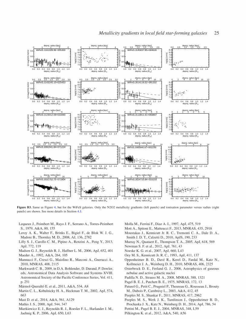
Metallicity gradients in local field star-forming galaxies 25
0.0 0.2 0.4 0.6 0.8 1.0 1.2 1.4deproj. radius [R25]
8.0
8.5
9.0
9.5
12+
log(
O/H
) N
2O2
0 1 2 3 4deproj. radius [kpc]
WiFeS:J161328.96−005300
0.0 0.2 0.4 0.6 0.8 1.0 1.2 1.4deproj. radius [R25
7.07.27.47.67.88.08.2
log(
q) [c
m/s
]
0 1 2 3 4deproj. radius [kpc]
0.0 0.2 0.4 0.6 0.8 1.0 1.2 1.4deproj. radius [R25]
8.0
8.5
9.0
9.5
12+
log(
O/H
) N
2O2
0.0 0.5 1.0 1.5 2.0 2.5deproj. radius [kpc]
WiFeS:J145837.85+064630
0.0 0.2 0.4 0.6 0.8 1.0 1.2 1.4deproj. radius [R25
7.07.27.47.67.88.08.2
log(
q) [c
m/s
]
0.0 0.5 1.0 1.5 2.0 2.5deproj. radius [kpc]
0.0 0.2 0.4 0.6 0.8 1.0 1.2 1.4deproj. radius [R25]
8.0
8.5
9.0
9.5
12+
log(
O/H
) N
2O2
0.0 0.5 1.0 1.5 2.0 2.5 3.0deproj. radius [kpc]
WiFeS:J143245.15+025453
0.0 0.2 0.4 0.6 0.8 1.0 1.2 1.4deproj. radius [R25
7.07.27.47.67.88.08.2
log(
q) [c
m/s
]
0.0 0.5 1.0 1.5 2.0 2.5 3.0deproj. radius [kpc]
0.0 0.2 0.4 0.6 0.8 1.0 1.2 1.4deproj. radius [R25]
8.0
8.5
9.0
9.5
12+
log(
O/H
) N
2O2
0 2 4 6 8 10 12deproj. radius [kpc]
WiFeS:J014119.52−091332
0.0 0.2 0.4 0.6 0.8 1.0 1.2 1.4deproj. radius [R25
7.07.27.47.67.88.08.2
log(
q) [c
m/s
]
0 2 4 6 8 10 12deproj. radius [kpc]
0.0 0.2 0.4 0.6 0.8 1.0 1.2 1.4deproj. radius [R25]
8.0
8.5
9.0
9.5
12+
log(
O/H
) N
2O2
0 2 4 6deproj. radius [kpc]
WiFeS:J123012.09+033440
0.0 0.2 0.4 0.6 0.8 1.0 1.2 1.4deproj. radius [R25
7.07.27.47.67.88.08.2
log(
q) [c
m/s
]
0 2 4 6deproj. radius [kpc]
0.0 0.2 0.4 0.6 0.8 1.0 1.2 1.4deproj. radius [R25]
8.0
8.5
9.0
9.5
12+
log(
O/H
) N
2O2
0 1 2 3 4 5 6deproj. radius [kpc]
WiFeS:J113911.61+093807
0.0 0.2 0.4 0.6 0.8 1.0 1.2 1.4deproj. radius [R25
7.07.27.47.67.88.08.2
log(
q) [c
m/s
]
0 1 2 3 4 5 6deproj. radius [kpc]
0.0 0.2 0.4 0.6 0.8 1.0 1.2 1.4deproj. radius [R25]
8.0
8.5
9.0
9.5
12+
log(
O/H
) N
2O2
0.0 0.5 1.0 1.5 2.0 2.5 3.0deproj. radius [kpc]
WiFeS:J091041.84+071224
0.0 0.2 0.4 0.6 0.8 1.0 1.2 1.4deproj. radius [R25
7.07.27.47.67.88.08.2
log(
q) [c
m/s
]
0.0 0.5 1.0 1.5 2.0 2.5 3.0deproj. radius [kpc]
0.0 0.2 0.4 0.6 0.8 1.0 1.2 1.4deproj. radius [R25]
8.0
8.5
9.0
9.5
12+
log(
O/H
) N
2O2
0 2 4 6 8 10deproj. radius [kpc]
WiFeS:J085640.67+002230
0.0 0.2 0.4 0.6 0.8 1.0 1.2 1.4deproj. radius [R25
7.07.27.47.67.88.08.2
log(
q) [c
m/s
]
0 2 4 6 8 10deproj. radius [kpc]
0.0 0.2 0.4 0.6 0.8 1.0 1.2 1.4deproj. radius [R25]
8.0
8.5
9.0
9.5
12+
log(
O/H
) N
2O2
0 5 10 15 20deproj. radius [kpc]
WiFeS:J031752.75−071804
0.0 0.2 0.4 0.6 0.8 1.0 1.2 1.4deproj. radius [R25
7.07.27.47.67.88.08.2
log(
q) [c
m/s
]
0 5 10 15 20deproj. radius [kpc]
0.0 0.2 0.4 0.6 0.8 1.0 1.2 1.4deproj. radius [R25]
8.0
8.5
9.0
9.5
12+
log(
O/H
) N
2O2
0 2 4 6 8 10deproj. radius [kpc]
WiFeS:J024710.84−010233
0.0 0.2 0.4 0.6 0.8 1.0 1.2 1.4deproj. radius [R25
7.07.27.47.67.88.08.2
log(
q) [c
m/s
]
0 2 4 6 8 10deproj. radius [kpc]
Figure B3. Same as Figure 4, but for the WiFeS galaxies. Only the N2O2 metallicity gradients (left panels) and ionisation parameter versus radius (right
panels) are shown. See more details in Section 4.1.
Lequeux J., Peimbert M., Rayo J. F., Serrano A., Torres-Peimbert
S., 1979, A&A, 80, 155
Leroy A. K., Walter F., Brinks E., Bigiel F., de Blok W. J. G.,
Madore B., Thornley M. D., 2008, AJ, 136, 2782
Lilly S. J., Carollo C. M., Pipino A., Renzini A., Peng Y., 2013,
ApJ, 772, 119
Madsen G. J., Reynolds R. J., Haffner L. M., 2006, ApJ, 652, 401
Maeder A., 1992, A&A, 264, 105
Mannucci F., Cresci G., Maiolino R., Marconi A., Gnerucci A.,
2010, MNRAS, 408, 2115
Markwardt C. B., 2009, in D.A. Bohlender, D. Durand, P. Dowler,
eds, Astronomical Data Analysis Software and Systems XVIII.
Astronomical Society of the Pacific Conference Series, Vol. 411,
p. 251
Marmol-Queralto E. et al., 2011, A&A, 534, A8
Martin C. L., Kobulnicky H. A., Heckman T. M., 2002, ApJ, 574,
663
Mast D. et al., 2014, A&A, 561, A129
Mathis J. S., 2000, ApJ, 544, 347
Mierkiewicz E. J., Reynolds R. J., Roesler F. L., Harlander J. M.,
Jaehnig K. P., 2006, ApJ, 650, L63
Molla M., Ferrini F., Diaz A. I., 1997, ApJ, 475, 519
Mott A., Spitoni E., Matteucci F., 2013, MNRAS, 435, 2918
Moustakas J., Kennicutt Jr. R. C., Tremonti C. A., Dale D. A.,
Smith J. D. T., Calzetti D., 2010, ApJS, 190, 233
Murray N., Quataert E., Thompson T. A., 2005, ApJ, 618, 569
Newman S. F. et al., 2012, ApJ, 761, 43
Noeske K. G. et al., 2007, ApJ, 660, L43
Oey M. S., Kennicutt Jr. R. C., 1993, ApJ, 411, 137
Oppenheimer B. D., Dave R., Keres D., Fardal M., Katz N.,
Kollmeier J. A., Weinberg D. H., 2010, MNRAS, 406, 2325
Osterbrock D. E., Ferland G. J., 2006, Astrophysics of gaseous
nebulae and active galactic nuclei
Padilla N. D., Strauss M. A., 2008, MNRAS, 388, 1321
Pagel B. E. J., Patchett B. E., 1975, MNRAS, 172, 13
Paturel G., Petit C., Prugniel P., Theureau G., Rousseau J., Brouty
M., Dubois P., Cambresy L., 2003, A&A, 412, 45
Peeples M. S., Shankar F., 2011, MNRAS, 417, 2962
Peeples M. S., Werk J. K., Tumlinson J., Oppenheimer B. D.,
Prochaska J. X., Katz N., Weinberg D. H., 2014, ApJ, 786, 54
Pettini M., Pagel B. E. J., 2004, MNRAS, 348, L59
Pilkington K. et al., 2012, A&A, 540, A56

26 Ho et al.
Pilyugin L. S., Grebel E. K., Mattsson L., 2012, MNRAS, 424,
2316
Pilyugin L. S., Grebel E. K., Kniazev A. Y., 2014, AJ, 147, 131
Pipino A., Lilly S. J., Carollo C. M., 2014, MNRAS, 441, 1444
Prantzos N., Boissier S., 2000, MNRAS, 313, 338
Queyrel J. et al., 2012, A&A, 539, A93
Recchi S., Spitoni E., Matteucci F., Lanfranchi G. A., 2008, A&A,
489, 555
Rich J. A., Torrey P., Kewley L. J., Dopita M. A., Rupke D. S. N.,
2012, ApJ, 753, 5
Rosales-Ortega F. F., Kennicutt R. C., Sanchez S. F., Dıaz A. I.,
Pasquali A., Johnson B. D., Hao C. N., 2010, MNRAS, 405, 735
Rosales-Ortega F. F., Sanchez S. F., Iglesias-Paramo J., Dıaz A. I.,
Vılchez J. M., Bland-Hawthorn J., Husemann B., Mast D., 2012,
ApJ, 756, L31
Roth M. M. et al., 2005, PASP, 117, 620
Rubin V. C., Ford Jr. W. K., Whitmore B. C., 1984, ApJ, 281, L21
Rupke D. S., Veilleux S., Sanders D. B., 2005a, ApJS, 160, 87
Rupke D. S., Veilleux S., Sanders D. B., 2005b, ApJS, 160, 115
Rupke D. S. N., Veilleux S., 2013, ApJ, 768, 75
Rupke D. S. N., Veilleux S., Baker A. J., 2008, ApJ, 674, 172
Rupke D. S. N., Kewley L. J., Barnes J. E., 2010a, ApJ, 710, L156
Rupke D. S. N., Kewley L. J., Chien L. H., 2010b, ApJ, 723, 1255
Salim S. et al., 2007, ApJS, 173, 267
Salpeter E. E., 1955, ApJ, 121, 161
Sanchez S. F. et al., 2012a, A&A, 538, A8
Sanchez S. F. et al., 2012b, A&A, 546, A2
Sanchez S. F. et al., 2014, A&A, 563, A49
Sanders R. L. et al., 2014, ArXiv e-prints
Savaglio S. et al., 2005, ApJ, 635, 260
Schlegel D. J., Finkbeiner D. P., Davis M., 1998, ApJ, 500, 525
Searle L., Sargent W. L. W., 1972, ApJ, 173, 25
Skillman E. D., Kennicutt R. C., Hodge P. W., 1989, ApJ, 347,
875
Skrutskie M. F. et al., 2006, AJ, 131, 1163
Spitoni E., Calura F., Matteucci F., Recchi S., 2010, A&A, 514,
A73
Springel V., Hernquist L., 2003, MNRAS, 339, 289
Steidel C. C., Erb D. K., Shapley A. E., Pettini M., Reddy N.,
Bogosavljevic M., Rudie G. C., Rakic O., 2010, ApJ, 717, 289
Steidel C. C. et al., 2014, ArXiv e-prints
Swinbank A. M., Sobral D., Smail I., Geach J. E., Best P. N.,
McCarthy I. G., Crain R. A., Theuns T., 2012, MNRAS, 426,
935
Tacconi L. J. et al., 2010, Nature, 463, 781
Tacconi L. J. et al., 2013, ApJ, 768, 74
Torrey P., Cox T. J., Kewley L., Hernquist L., 2012, ApJ, 746, 108
Tremonti C. A. et al., 2004, ApJ, 613, 898
van Zee L., Salzer J. J., Haynes M. P., O’Donoghue A. A.,
Balonek T. J., 1998, AJ, 116, 2805
Vazdekis A., Sanchez-Blazquez P., Falcon-Barroso J., Cenarro
A. J., Beasley M. A., Cardiel N., Gorgas J., Peletier R. F., 2010,
MNRAS, 404, 1639
Veilleux S., Osterbrock D. E., 1987, ApJS, 63, 295
Veilleux S., Cecil G., Bland-Hawthorn J., 2005, ARA&A, 43, 769
Vila-Costas M. B., Edmunds M. G., 1992, MNRAS, 259, 121
Walcher C. J. et al., 2014, A&A, 569, A1
Weiner B. J. et al., 2009, ApJ, 692, 187
Werk J. K., Putman M. E., Meurer G. R., Santiago-Figueroa N.,
2011, ApJ, 735, 71
Woosley S. E., Weaver T. A., 1995, ApJS, 101, 181
Wuyts E. et al., 2014, ApJ, 789, L40
Wyse R. F. G., Silk J., 1985, ApJ, 296, L1
Yates R. M., Kauffmann G., Guo Q., 2012, MNRAS, 422, 215
York D. G. et al., 2000, AJ, 120, 1579
Yuan T. T., Kewley L. J., Swinbank A. M., Richard J., Livermore
R. C., 2011, ApJ, 732, L14
Yuan T. T., Kewley L. J., Rich J., 2013, ApJ, 767, 106
Zahid H. J., Kewley L. J., Bresolin F., 2011, ApJ, 730, 137
Zahid H. J., Dima G. I., Kewley L. J., Erb D. K., Dave R., 2012,
ApJ, 757, 54
Zahid H. J., Geller M. J., Kewley L. J., Hwang H. S., Fabricant
D. G., Kurtz M. J., 2013, ApJ, 771, L19
Zahid H. J., Torrey P., Vogelsberger M., Hernquist L., Kewley L.,
Dave R., 2014a, Ap&SS, 349, 873
Zahid H. J. et al., 2014b, ApJ, 792, 75
Zahid H. J., Dima G. I., Kudritzki R. P., Kewley L. J., Geller M. J.,
Hwang H. S., Silverman J. D., Kashino D., 2014c, ApJ, 791, 130
Zaritsky D., Kennicutt Jr. R. C., Huchra J. P., 1994, ApJ, 420, 87


![Metallicity gradients in Local Universe galaxies: time · PDF filearXiv:1602.02529v1 [astro-ph.GA] 8 Feb 2016 Astronomy&Astrophysicsmanuscript no. magrini_final_080216 c ESO 2016](https://cdn.vdocuments.net/doc/165x107/5a857d507f8b9afc5d8c6d89/metallicity-gradients-in-local-universe-galaxies-time-160202529v1-astro-phga.jpg)