
NEER ENGI
MID-TERM REPORT: COMPLEX VENTILATION AND MICRO-ENVIRONMENTAL CONTROL IN LIVESTOCK HOUSING Civil and Architectural Engineering Technical Report CAE-TR-2

DATA SHEET Title: Mid-term report: Complex Ventilation and Micro-Environmental Control in Livestock Housing Subtitle: Civil and Architectural Engineering Series title and no.: Technical report CAE-TR-2 Author: Hao Li, Department of Engineering – Civil and Architectural Engineering, Aarhus University Internet version: The report is available in electronic format (pdf) at the Department of Engineering website http://www.eng.au.dk. Publisher: Aarhus University© URL: http://www.eng.au.dk Year of publication: 2015 Pages: 25 Editing completed: April 2015 Abstract: Micro-complex ventilation involves integrating preci-sion local ventilations in animal zones. In order to gain knowledge about air motion and temperature distribution in an-imal occupied zones, the project will investigate an integrated micro ventilation concept in livestock housing. Data will be gathered by using both Computational Fluid Dynamics (CFD) simulations and scale experiments in wind tunnel. After the es-tablishment of the system, optimisations are also needed. Then, to validate the optimal system, varied techniques including lo-cal cross ventilation, tunnel ventilation, low pressure ventilation and heat exchange will be investigated. The proposed system combines the advantages of natural, mechanical and dis-placement ventilation, making it a technology with great effi-ciency and potential. So far, parts of the experiment about the heated body have al-ready been conducted in the wind tunnel. A CFD simulation about heat convection from chicken have already been fin-ished and written into a manuscript. This report contains intro-duction of the project of Complex Ventilation and Micro-Environmental Control in Livestock Housing. This report contains activities, courses, and manuscript was presented. There is also a plan for further work. Keywords: Ventilation, Climate control, Thermal condition, Ex-perimental fluid dynamic, Computational fluid dynamic Supervisor: Guoqiang Zhang Financial support: Aarhus University/China scholarship council Please cite as: Hao Li, 2015. Complex Ventilation and Micro-Environmental Control in Livestock Housing. Department of En-gineering, Aarhus University. Denmark. 25 pp. - Technical report CAE -TR-2 Layout: Hao Li Cover image: Hao Li ISSN 2246-0942 Reproduction permitted provided the source is explicitly acknowledged

MID-TERM REPORT:
COMPLEX VENTILATION AND MICRO-ENVIRONMENTAL CONTROL
IN LIVESTOCK HOUSING Hao Li
Aarhus University, Department of Engineering
Abstract Micro-complex ventilation involves integrating precision local ventilations in animal zones. In order to gain knowledge about air motion and temperature distribution in animal occupied zones, the project will investigate an integrated micro ventilation concept in livestock housing. Data will be gathered by using both Computational Fluid Dynamics (CFD) simulations and scale experiments in wind tunnel. After the establishment of the system, optimisations are also needed. Then, to validate the optimal system, varied techniques including local cross ventilation, tunnel ventilation, low pressure ventilation and heat exchange will be investigated. The proposed system combines the advantages of natural, mechanical and displacement ventilation, making it a technology with great efficiency and potential. So far, parts of the experiment about the heated body have already been conducted in the wind tunnel. A CFD simulation about heat convection from chicken have already been finished and written into a manuscript. This report contains introduction of the project of Complex Ventilation and Micro-Environmental Control in Livestock Housing. This report contains activities, courses, and manuscript was presented. There is also a plan for further work.

Complex Ventilation and Micro-Environmental Control in Livestock
Housing
Hao Li
Summary
Micro-complex ventilation involves integrating precision local ventilations in animal zones. In order to
gain knowledge about air motion and temperature distribution in animal occupied zones, the project
will investigate an integrated micro ventilation concept in livestock housing. Data will be gathered by
using both Computational Fluid Dynamics (CFD) simulations and scale experiments in wind tunnel.
After the establishment of the system, optimisations are also needed. Then, to validate the optimal
system, varied techniques including local cross ventilation, tunnel ventilation, low pressure ventilation
and heat exchange will be investigated. The proposed system combines the advantages of natural,
mechanical and displacement ventilation, making it a technology with great efficiency and potential.
So far, parts of the experiment about the heated body have already been conducted in the wind tunnel.
A CFD simulation about heat convection from chicken have already been finished and written into a
manuscript. This report contains introduction of the project of Complex Ventilation and Micro-
Environmental Control in Livestock Housing. The work progress including activities, courses, and
manuscript was presented. There is also a plan for further work.
1. Introduction to the field of research
Research on animal behaviour and welfare have showed that both thermal and airflow parameters have
strong influence on the procedures of livestock breeding. A poor thermal environment results in a
negative spiral of development for animals, personnel, environment, economy and food quality
prompted by reduced hygiene, increased risk of diseases, increased ammonia evaporation, reduced air
quality and increased daily labour requirement for pen cleaning. While on the other hand ventilation
1
and airflow at animal zone could have large effects on ammonia and greenhouse gas emission from
livestock buildings.
The purpose of the ventilation system is to maintain a desired indoor thermal condition while
controlling levels of humidity and removing gaseous contaminants introduced by the animal and their
waste (Saha et al., 2010). Houses can be acclimated through either forced or natural ventilation. Natural
ventilation is one of the techniques for lower energy consumption compared with the energy
consumption of forced ventilation (Ecim-Djuric, 2009). However, at certain circumstances, only
depending on natural ventilation is not enough to meet the requirement of air motion in animal
buildings. Then the mechanical ventilation is needed. There are many different kinds of ventilation
system in a mechanical ventilated animal building, e.g. tunnel ventilation, low pressure ventilation, and
cross ventilation. These ventilation systems could be installed either singly or integratedly in animal
buildings. All these lead to a complex both air velocity and temperature distributions in animal occupy
zone, and the control of the indoor environment become correspondingly complex. That is the basic
complex ventilation idea. It derives from a study on a pig building conducted by Farm Building
Division of Danish Building Research Institute in 1990s (Strøm and Zhang 1989; Zhang et al. 1992).
Until now many researches have been done on complex ventilation system. However, there are still
many conceptions are unclear.
2. Hypothesis/Aim of the project
Different control strategies could result to different indoor environments and have varied cooling
potentials during the hot period. The integral impact from environment will affect animal comfort on
varied degrees. To provide a friendly environment to the animals, it is necessary to find a reliable
parameter to represent animals’ comfort first and then try to reach the set environment through
different strategies. The research then could be separate into two parts, one is to explore the thermal
index for animal, and the other is to study indoor climate parameters results from different ventilation
systems.
The aims of the project are 1) to introduce a new concept for monitoring the thermal and airflow
conditions in the animal zone, 2) and then to set up a dynamic predictive model to provide a precision
2

environment control strategy at individual animal or defined zone level and consequently to improve
animal welfare and to reduce environmental impact, 3) to generate knowledge on cooling effectiveness
of different kinds of cooling and ventilation systems.
3. Description of methods
The project will apply both numerical modelling method and full scale experiments to investigate the
effectiveness of the system for an optimal thermal environment and air quality for both animal and
workers with high effectiveness and low energy consumption.
Models of heated bodies which are so-called artificial pig and poultry will be made and test in wind
tunnel in Air Physics Lab, Aarhus University, Denmark. This wind tunnel has a large range of
turbulence boundary layers and dimensions height ×width ×length=6.00m×1.38m×1.55m. This low-
speed-type wind tunnel can produce a maximum flow with a wind speed of 3.8m/s.
Computational Fluid Dynamics (CFD) can effectively model airflow in both spatial and temporal fields,
and it was proved the potential to model livestock buildings and can provide concrete flow information.
Therefore, in this project, CFD is used to analyse the air motion and thermal condition in AOZ and heat
boundary of animals.
4. Progress of the project
Two heated body with different sizes have been built. Heat convective coefficients of the cylinders on
different air velocities and orientations have been generated through experiment. That data could be
used as basic data to develop the effective temperature of animals.
CFD simulation on a model chicken was also conducted to test the feasibility of using CFD method to
study heat transfer convective coefficient from animals. Great potential have been showing in the
research. The results have been arranged in a manuscript.
Both the simulation and experiment will focus on more complex geometry in future research.
5. Dissemination
3

5.1. Publications
Li, H., Zhang, G., 2015. A numerical approach to study forced convection from animal: simulation
with a real geometry. Manuscript for publication in a scientific journal.
Zong, C., Li, H., Zhang, G., 2014. Ammonia and greenhouse gas emissions from fattening pig house
with two types of partial pit ventilation systems. Agriculture, Ecosystems & Environment, Revised
version submitted in Oct. 2014.
Zong, C., Li, H., Zhang, G., 2014. Airflow characteristics in a pig house with partial pit ventilation
system: an experimental chamber study. Prepared submitting to a peer review journal.
Zong, C., Zhang, G., Li, H., Rong, L. 2014. Investigation on ventilation effectiveness in a full-scale
model pig house with partial pit ventilation system. Proceedings International Conference of
Agricultural Engineering, Zurich, 06-10.07.2014.
Yan, Z., Wang, C., Li, B., Zhang, G., Shi, Z., Li, H., Wang, H. Yuan, Y. Influence of water
temperature and spraying interval on cooling effect of sprinkler system in dairy barns. Applied
Engineering in Agriculture, Vol. 30(4): 611-617.
5.2. Activities
Experiment, report and discussion with VSP (pig research center) on design of ventilation systems for
point extraction, from 01/10/2013 to 05/03/2014, in Denmark
Seminar on application of CFD in agriculture, 09/04/2014, in Korea
Workshop on the CFD simulation for ventilation system, 19/05/2014, in Korea
Seminar on hot climate control in Pig & poultry house, 16/10/2014, in Denmark
Seminar on heat balance model in animals, 27/10/2014, in Denmark
Seminar on hot climate control and technology in Pig & poultry housing, 14/01/2015, in Denmark
4

5.3. Courses
Completed Courses: 20.5 ECTS; Ongoing: 4 ECTS; Planned: 7 ECTS; In total: 31.5 ECTS.
5.4. Study abroad:
I spent 3 months in the lab of Prof. In-bok Lee in Aero-Environmental & Energy Engineering, College
of Agriculture and Life Sciences, Seoul National University. There I developed my CFD simulation
skills and communicated research status with peers.
6. Plan for remaining study period
6.1. Conference
Course title Institution ECTS Status
Fundamentals of Ventilation, Indoor Air
Quality, Air Motion and Emissions (MD 1) Aarhus University 5 Completed
Science Teaching -Module 1:Introduction to
Science Teaching Aarhus University 3 Completed
Academic English for non-Danish Speaking
PhD Students Aarhus University 3 Completed
Fundamental of computational fluid dynamics
(CFD) Aalborg University 3.5 Completed
Computing with data using R Aalborg University 4 Completed
Introduction to R Aarhus University 1 Completed
Basic Statistical analysis in Life and
Environmental Sciences Aarhus University 4 Ongoing
Fundamentals of Ventilation, Indoor Air
Quality, Air Motion and Emissions (MD 2) Aarhus University 5
Planned,
June 2015
The World of Research Aarhus University 2 Planned,
May 2015
5

I plan to join two international conferences. The first one is the ASABE annual conference 2015 in
New Orleans, Louisiana, US. And the second one is CIGR conference 2016 in Aarhus, Denmark. I will
make oral presentations there.
6.2. Working plan on research
For the next half period for my PhD study, I plan to do the research in two different levels – the
housing level and animal level. On the housing level the core of research is to study the effectiveness of
different ventilation and cooling system. On the animal level, the goal is to develop the index that could
represent real feeling of animal in different thermal conditions.
Working title in housing level:
1. Modelling indoor environment and cooling potential with different cooling strategies in closed
animal housing (expect to be started from March 2015 and finished in June 2015)
2. Economic analysis on the cooling strategies in different climate zones (air conditioner, natural
ventilation and mechanical ventilation) (expect to be started from April 2015 and finished in
August 2015)
Working title in animal level:
1. Scale effect on convective heat loss – a study based on heated bodies (expect to be finished in
March 2015)
2. Comparison of convective coefficient between pig model with real and simplified shapes (expect
to be finished in March 2016)
3. A numerical approach to study forced convection from animal: simulation with a fur layer
(expect to be finished in June 2016)
It is planned that each working title will produce one publication.
6

Appendix A: Manuscript “A numerical approach to study forced convection from animal: simulation with a real
geometry”
7
A numerical approach to study forced convection from animal: simulation 1
with a real geometry 2
Hao Li, Guoqiang Zhang 3
Department of Engineering, Aarhus University, Blichers Allé 20, P. O. Box 50, 8830 Tjele, Denmark 4
5
Abstract 6
Convective heat transfer is an important parameter to judge animal thermal comfort. Computational 7
Fluid Dynamics (CFD) method was employed to study convective coefficient from animal. In order to 8
achieve accurate result, several RANS (Reynolds averaged Navier-Stokes) turbulence models were 9
tested on a sphere model for the feasibility to study forced convection using CFD method. RSM model 10
showed the best agreement with theoretical calculation and therefore was adopted for further 11
calculation. The results of simulation showed the CFD method had a strong potential in studying 12
convective coefficient of animal. Based on the simulation result, convective coefficient of chicken was 13
predicted over a broader range of air velocity compared with former research. A relationship between 14
model with a chicken geometry and sphere was also discussed in the paper. 15
16
1. Introduction 17
Thermal comfort is an important factor for farm animal. Poor thermal condition may lead to stress of 18
animals and even to death of animals, and poor production. The thermal comfort of animal is highly 19
dependent on heat transfer from animal to the environment. The heat transfer from animal is including 20
evaporation, conduction, convection and radiation. Among all these four kinds of heat transfer avenues 21
convection is one of the most important, since it is highly relevant to the control of the ventilation air 22
speed in animal occupied zone. 23
Many researches have been conducted using varied artificial animal models to study the thermal 24
condition of animals. Most study in those works, Spheres and cylinders were employed for physical 25
modelling (Bakken, 1976; Bakken and Gates, 1975; Campbell and Norman, 1998; Monteith and 26
Unsworth, 2013; Norton et al., 2010; Porter and Gates, 1969) . The oversimplification of the geometry 27
will undoubtedly lead to discrepancy on the results. Wathes and Clark (1981) tested heat transfer from 28
a copper model in a chicken model and Mitchell (1985) tested the convective coefficient of a real 29
chicken using a wind-tunnel calorimeter. However, both of the experiment had some limitations. They 30
were not conducted in a very high wind speed. The air pattern around animals could not get due to the 31
limitation of the equipment. 32
8

CFD has become a useful and powerful tool to predict airflow characteristics and mass and energy 33
transfer across wide research areas: airflow distribution in greenhouses (Bartzanas et al., 2002); 34
ammonia emission from pig houses(Rong et al., 2010); dynamic flux chamber methodology (Saha et al., 35
2011); pit exhaust system of a cow building; remove ratio of gases (Wu et al, 2012); Air flow pattern 36
inside a small cow room (Gebremedhin and Wu, 2005); the indoor environment of a pig building (Seo 37
et al, 2011). 38
To determine convective coefficient of a bluff body in a ventilated air space, it is depending on the 39
modelling results in both the air velocity field and the temperature field. The accuracies of both aspects 40
have influence on the final result. And the two aspects could have interaction for the simulation of the 41
convective coefficient. Zhang, Zhai et al. (2007) tested different turbulence models in enclosed space, 42
the predictions on temperature, velocity and turbulence are in different accuracy levels. From this point, 43
turbulence models need to evaluated for the prediction of convective coefficient. 44
Therefore, the objective of this study is 1) to assess the feasibility of using CFD (computational Fluid 45
Dynamic) to study forced convection from animals, 2) to use CFD model to make prediction of 46
convective coefficients on higher air velocity, 3) to explore the relationship between sphere and the 47
model in a chicken shape. 48
2. Materials and Methods 49
2.1. Geometry and calculation domain 50
Firstly, a model chicken was made based on real geometry of chicken by Sketchup (Google Inc., USA). 51
However, too detailed model could result to increasing of difficulty in mesh establishment and burden 52
in calculation afterwards. Therefore, the model was rebuild and appropriately simplified in Rhino 53
(Robert McNeel & Assoc Inc., USA); the comb and legs were removed, and beak and wings were 54
moderately smoothed (Fig. 1). The model was rescaled to a size with a surface area of 0.0769m2 which 55
is the calculated surface area of chicken in a former experiment (Mitchell, 1985) . 56
57 Fig. 1 The process of generating the model chicken
9

The simulated wind tunnel was following the dimensions in Mitchell’s experiment as well, the length 58
was 1m, and the cross section was 0.31m*0.31m. Model chicken was placed in the middle with a 59
height of 0.06m from floor. That height was corresponding length of leg in that growing period. Four 60
chicken orientations respect to the wind were set in the simulation, 0o (Fig. 2 a), 45
o (Fig. 2 b), 90
o (Fig. 61
2 c) and 180o (Fig. 2 d), respectively. 62
63
In order to study scale effect on the results, the calculation domain was scaled into two other sizes by 64
factors of 0.6 and 1.3. The corresponding areas of chicken surface were 0.0276 m2 and 0.1300 m
2, 65
respectively. In all the three scales, the body weight was calculated from the surface area from the 66
relationship below (Walsberg, 1978): 67
0.667 / 0.081M S 68
The corresponding body weights were 0.2kg, 0.9kg, and 2.0kg, respectively, which respected the whole 69
growth process of a chicken. 70
Fig. 2 Schematic of the calculation domains with four chicken orientations to the wind: (a) 0°, trunk
axis parallel to the wind direction with head facing the wind; (b) 45°, trunk axis 45° angle to the wind
direction; (c) 90°, Trunk axis perpendicular to wind direction; (d) 180°, trunk axis parallel to the wind
direction with posterior end facing the wind.
( a )
( d )
( b )
( c )
10

In order to test the accuracy of CFD method in studying forced convection, a simple geometry of 71
sphere was examined in a same virtual wind tunnel. The sphere had a diameter of 15.6cm and the area 72
was 0.0769 m2, as same as the virtual chicken in this study. The sphere was arranged in the middle of 73
virtual tunnel. 74
2.2. Basic concept of CFD and software 75
The fundamental bases of almost all CFD problems are to solve governing equations like the Navier-76
Stokes and continuity equations. All these governing equations mentioned above can be written in a 77
general form as: 78
( )( ) ( )div div grad S
t
u 79
Written in expansion, 80
( ) ( ) ( ) ( )( ) ( ) ( )
div u div v div wS
t x y y x x y y z z
81
where, represents variables, the effective diffusion coefficient, and S the source term of an equation. 82
The terms are transient term, convective term, diffusive term, and source term, respectively in equation. 83
In this research, commercial software Fluent 15.0 (Ansys Inc., USA) was used to solve the equations 84
on the basis of finite volume method. Standard k-ε, RNG k-ε, low Re k-ε, transition SST and RSM 85
turbulence models were tested in this work. Velocity and turbulence terms for convection were all 86
approximated using second order upwind scheme. Diffusion terms were discretised using central 87
difference scheme. SIMPLE method was employed for the pressure-velocity correction. 88
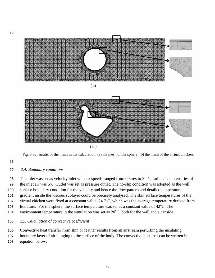
2.3. Mesh 89
To solve the boundary layer around the virtual chicken, continuously layers of prism cells were created 90
both on the surface of the virtual chicken and wall with an initial height of 0.1mm to keep the y+<1. 91
Tetra-meshes were then arranged from the outside of the boundary layer to the other side walls in the 92
analytical space. After the grid independence test, a total number of computational cells of 1.5 million 93
were used for the mesh of sphere and virtual chicken. 94
11
95
96
2.4. Boundary conditions 97
The inlet was set as velocity inlet with air speeds ranged from 0.3m/s to 3m/s, turbulence intensities of 98
the inlet air was 5%. Outlet was set as pressure outlet. The no-slip condition was adopted as the wall 99
surface boundary condition for the velocity and hence the flow pattern and detailed temperature 100
gradient inside the viscous sublayer could be precisely analysed. The skin surface temperatures of the 101
virtual chicken were fixed at a constant value, 24.7oC, which was the average temperature derived from 102
literature. For the sphere, the surface temperature was set as a constant value of 42oC. The 103
environment temperature in the simulation was set as 20oC, both for the wall and air inside. 104
2.5. Calculation of convective coefficient 105
Convective heat transfer from skin or feather results from an airstream perturbing the insulating 106
boundary layer of air clinging to the surface of the body. The convective heat loss can be written in 107
equation below: 108
( a)
( b )
Fig. 3 Schematic of the mesh in the calculation: (a) the mesh of the sphere; (b) the mesh of the virtual chicken.
12
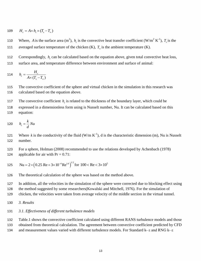
( ) c c sH A h T T 109
Where, A is the surface area (m2),
ch is the convective heat transfer coefficient (W/m2 K
-1),
sT is the 110
averaged surface temperature of the chicken (K), T is the ambient temperature (K). 111
Correspondingly, ch can be calculated based on the equation above, given total convective heat loss, 112
surface area, and temperature difference between environment and surface of animal: 113
( )
cc
s
Hh
A T T 114
The convective coefficient of the sphere and virtual chicken in the simulation in this research was 115
calculated based on the equation above. 116
The convective coefficient ch is related to the thickness of the boundary layer, which could be 117
expressed in a dimensionless form using is Nusselt number, Nu. It can be calculated based on this 118
equation: 119
c
kh Nu
d 120
Where k is the conductivity of the fluid (W/m K-1
), d is the characteristic dimension (m), Nu is Nusselt 121
number. 122
For a sphere, Holman (2008) recommended to use the relations developed by Achenbach (1978) 123
applicable for air with Pr = 0.71: 124
1/2
4 1.6Nu 2 0.25 Re 3 10 Re for 5100 Re 3 10 125
The theoretical calculation of the sphere was based on the method above. 126
In addition, all the velocities in the simulation of the sphere were corrected due to blocking effect using 127
the method suggested by some researchers(Kowalski and Mitchell, 1976). For the simulation of 128
chicken, the velocities were taken from average velocity of the middle section in the virtual tunnel. 129
3. Results 130
3.1. Effectiveness of different turbulence models 131
Table.1 shows the convective coefficient calculated using different RANS turbulence models and those 132
obtained from theoretical calculation. The agreement between convective coefficient predicted by CFD 133
and measurement values varied with different turbulence models. For Standard k- ε and RNG k- ε 134
13
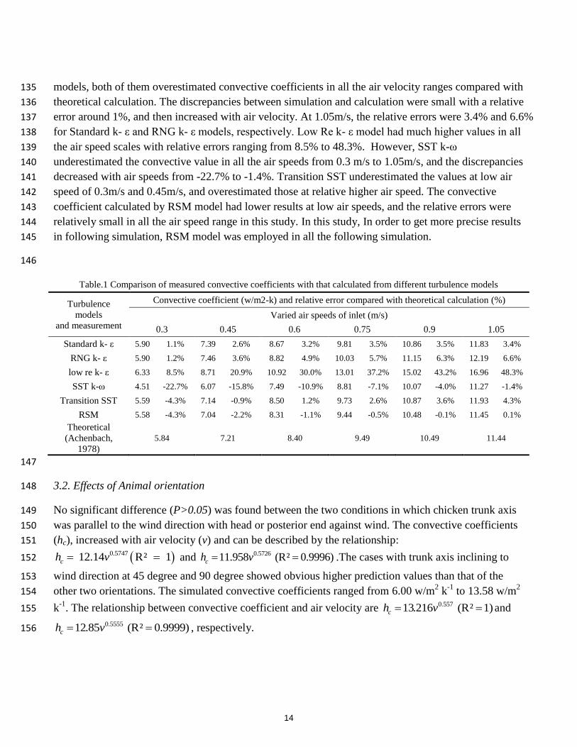
models, both of them overestimated convective coefficients in all the air velocity ranges compared with 135
theoretical calculation. The discrepancies between simulation and calculation were small with a relative 136
error around 1%, and then increased with air velocity. At 1.05m/s, the relative errors were 3.4% and 6.6% 137
for Standard k- ε and RNG k- ε models, respectively. Low Re k- ε model had much higher values in all 138
the air speed scales with relative errors ranging from 8.5% to 48.3%. However, SST k-ω 139
underestimated the convective value in all the air speeds from 0.3 m/s to 1.05m/s, and the discrepancies 140
decreased with air speeds from -22.7% to -1.4%. Transition SST underestimated the values at low air 141
speed of 0.3m/s and 0.45m/s, and overestimated those at relative higher air speed. The convective 142
coefficient calculated by RSM model had lower results at low air speeds, and the relative errors were 143
relatively small in all the air speed range in this study. In this study, In order to get more precise results 144
in following simulation, RSM model was employed in all the following simulation. 145
146
Table.1 Comparison of measured convective coefficients with that calculated from different turbulence models
Turbulence
models
and measurement
Convective coefficient (w/m2-k) and relative error compared with theoretical calculation (%)
Varied air speeds of inlet (m/s)
0.3 0.45 0.6 0.75 0.9 1.05
Standard k- ε 5.90 1.1% 7.39 2.6% 8.67 3.2% 9.81 3.5% 10.86 3.5% 11.83 3.4%
RNG k- ε 5.90 1.2% 7.46 3.6% 8.82 4.9% 10.03 5.7% 11.15 6.3% 12.19 6.6%
low re k- ε 6.33 8.5% 8.71 20.9% 10.92 30.0% 13.01 37.2% 15.02 43.2% 16.96 48.3%
SST k-ω 4.51 -22.7% 6.07 -15.8% 7.49 -10.9% 8.81 -7.1% 10.07 -4.0% 11.27 -1.4%
Transition SST 5.59 -4.3% 7.14 -0.9% 8.50 1.2% 9.73 2.6% 10.87 3.6% 11.93 4.3%
RSM 5.58 -4.3% 7.04 -2.2% 8.31 -1.1% 9.44 -0.5% 10.48 -0.1% 11.45 0.1%
Theoretical
(Achenbach,
1978)
5.84 7.21 8.40 9.49 10.49 11.44
147
3.2. Effects of Animal orientation 148
No significant difference (P>0.05) was found between the two conditions in which chicken trunk axis 149
was parallel to the wind direction with head or posterior end against wind. The convective coefficients 150
(hc), increased with air velocity (v) and can be described by the relationship: 151
0.5747 12.14 R² 1 ch v and 0.572611.958 (R² 0.9996) ch v .The cases with trunk axis inclining to 152
wind direction at 45 degree and 90 degree showed obvious higher prediction values than that of the 153
other two orientations. The simulated convective coefficients ranged from 6.00 w/m2 k
-1 to 13.58 w/m
2 154
k-1
. The relationship between convective coefficient and air velocity are 0.55713.216 (R² 1) ch v and155
0.555512.85 (R² 0.9999) ch v , respectively. 156
14

The cases with trunk axis parallel to the wind with head towards wind were similar to the experiment 157
done by Wathes and Clark (1981). The CFD simulation results showed that the convective coefficients 158
were underestimated at lower air speeds but overestimated at higher air speeds. The relative errors 159
ranged from -8.8% to 5.2%. ANOVA analysis showed that the difference between these two group data 160
was not significant (P>0.05).The cases that with lateral orientation to the air flow were in the same 161
conditions with the experiment done by Mitchell (1985). The mean deviation between simulation and 162
experiment was -8.42% with the largest discrepancies occurring at the very lowest and very highest air 163
velocities. ANOVA analysis showed a significant difference between these two group data (P<0.05). 164
165
166
3.3. Effects of the model scale 167
Fig.5 shows the convective coefficient of chicken models with different scales calculated over the 168
range of air speeds in simulation. It is obviously that the models with smaller scale have higher 169
convective coefficient compared larger scale models in the same air velocities. The model with 0.9kg 170
corresponding weight was the same model as the model with lateral orientation to the wind direction. 171
The relationship between convective coefficient and air velocity of the other two models can be 172
described as 0.544616.138 (R² 0.9999) ch v and hc=11.464v0.5621
(R² = 0.9998) for models in 0.2kg 173
and 2kg, respectively. 174
175
5.00
7.00
9.00
11.00
13.00
15.00
17.00
0.2 0.4 0.6 0.8 1 1.2
Co
nve
ctiv
e c
oe
ffic
ien
t, w
/m2
-k
Air speed, m/s
0°
45°
90°
180°
Experiment (Wathes and Clark, 1981)
Experiment (Mitchell, 1985)
Fig. 4 Relationship between air speed and convective coefficient with different orientations
15

176
177
3.4. Velocity field and airflow pattern around animals 178
Symmetry plane in calculation domain was employed to demonstrate the velocity field and airflow 179
patterns. Examples for velocity field are showed in Fig for 0° and 90° orientation to the airflow with 180
inlet air speeds of 0.3m/s and 1.05m/s. 181
In the cases of chicken head facing the wind, as showed in Fig.6 (a) and Fig. 6 (b), higher air velocities 182
appeared at the top and the bottom of the chicken body. There were low air velocity zones just behind 183
the neck and trunk of the chicken. In the cases that chicken were laterally orientating to the airflow, as 184
showed in Fig. 7(a) and Fig. 7(b), higher air velocities were observed also at the top and bottom 185
position of the virtual chicken. Obvious low air velocity zones were found downwind side of the body. 186
They had a much larger affected area compared with the cases with chicken head orientating to the 187
wind. The velocity contours were almost same in condition with 0.3m/s inlet air speed and 1.05m/s 188
inlet air speed. The air velocities were proportionate to the inlet air velocities. 189
Airflow patterns were demonstrated in Fig. 8. Small vortexes were found downwind side of the neck 190
and body in cases that chicken head orientating to the wind with inlet air velocity of 0.3m/s (Fig. 8 a) 191
and 1.05m/s (Fig. 8 b) . No significant difference of air pattern was found in these two cases. Large 192
vortex zones were found behind the body along wind direction in the cases that trunk axis 193
perpendicular to wind direction in the two velocities working conditions (Fig. 8 c and d). The vortex 194
zones were the place where were the low air velocity zones. 195
196
5
7
9
11
13
15
17
0.2 0.4 0.6 0.8 1 1.2
Co
nve
ctiv
e c
oe
ffic
ien
t, w
/m2
-k
Air speed, m/s
0.2kg
0.9kg
2kg
Experiment (Wathes and Clark, 1981)
Experiment (Mitchell, 1985)
Fig.5 Relationship between air speed and convective coefficient with different scales
16

197
Fig.6 Velocity field around chicken with 0° to the wind direction while the inlet
velocity of: ( a ) 0.3m/s; ( b ) 1.05m/s.
( b )
( a )
17

198
Fig.7 Velocity field around chicken with 90° to the wind direction while the inlet
velocity of: ( a ) 0.3m/s; ( b ) 1.05m/s.
( a )
( b )
18

199
3.5. Heat flux on the surface 200
Fig.9 shows that the heat flux from the surface of body in the cases with inlet air velocities of 0.3m/s 201
(Fig. 9 a) and 1.05m/s (Fig. 9 b) while chicken was facing the wind. Highest heat flux were found on 202
( a )
( b )
( c )
( d )
Fig.8 Airflow pattern around chicken with: (a) 0° to the wind direction while the inlet velocity
of 0.3m/s; (b) 0° to the wind direction while the inlet velocity of 1.05m/s; (c) 90° to the wind
direction while the inlet velocity of 0.3m/s; (b) 90° to the wind direction while the inlet velocity
of 1.05m/s;
( a )
19

the beak, the values were approxmately 111w/m2 and 203w/m
2, respectively, for the two velocity 203
0.3m/s and 1.05m/s. The heat flux were relatively higher on the windward side, and lower on the rest of 204
body. The average heat flux from the body surface were 30.4 w/m2 and 62.5w/m
2 in these two velocity 205
cases. 206
Fig. 10 shows that the heat flux from the chicken surface in the two velocity conditions with trunk axis 207
perpendicular to the wind. Higher heat flux were found on 2 locations, beak and tail on the leeward side, 208
on both the velocity working conditions. Hihgest value reached to around 105w/m2 and 195w/m
2 for 209
0.3m/s (Fig. 10 a) and 1.05m/s (Fig. 10 b) inlet velocity. The downwind sides of the surfaces were 210
found to have significant lower heat flux on both of the velocity cases.The mean heat flux from the 211
whole surface of body were 36.6w/ m2
(Fig. 10 c) and 73.5w/ m2
(Fig. 10 d) in the two cases. 212
213
Fig.9 Heat flux from the surface of body when the chicken was 0° to the wind direction in the cases with inlet
air velocity: (a) 0.3m/s and (b) 1.05m/s.
(a) (b)
20

214
3.6. Prediction of convective coefficient on higher air velocity 215
Convective coefficients at higher air velocities were predicted in cases with three orientations to the 216
wind, i.e., chicken trunk axis 0°, 45° and 90° to the wind direction. New regression curves were made 217
based on the simulated data in all the air velocities range from 0.3m/s to 3m/s. The relationships 218
between convective coefficients and air velocities were hc= 2.417v0.6216
(R² = 0.9983), hc = 13.478 v 219
0.6015 (R² = 0.9985) and hc = 13.087v
0.6141 (R² = 0.9975), respectively, for the trunk axis of 0°, 45° and 220
90° to the wind direction. In addition, a regression that depicting the general condition of chicken 221
between convective coefficient and air velocity was calculated based on the mean convective 222
coefficient of the three orientations. The curve could be described as hc= 12.994v0.6121
(R² = 1). 223
4. Discussion 224
4.1. Selection of RANS turbulence models 225
Fig.10 Heat flux from surface with trunk axis perpendicular to the wind in inlet air velocity of: (a) 0.3m/s on
windward side; (b) 1.05m/s on windward side; (c) 0.3m/s on leeward side; (d) 1.05m/s on leeward side.
(a) (b)
(c) (d)
21
In the preliminary study on the convective heat transfer from the sphere, Standard k- ε, Transition SST 226
and RSM models had relatively low relative errors within 5% in the simulation in comparison with 227
theoretical calculation. Compared with Standard k- ε model and Transition SST model, RSM model 228
generated more accuracy results in a broad range. It was reported that RSM model made a accurcy 229
results for velocity field(Wu et al., 2012). Since the convective coefficient is highly dependent on the 230
velocity and boundary layer, the precise simulation of velocity is appreciable in simulating the 231
convective coefficients. However, RSM model could take approximate five times more time in 232
calculation than Standard k- ε (Zhang et al., 2007). In this study, Transition SST needed 1.5 times 233
computing time longer than Standard k- ε. Taking computing time into consideration, Standard k- ε 234
model is one of the most time saving turbulence model with relative high accuracy in calculating 235
convective heat transfer. From this point, it is sufficient enough to carry out most of the calculation 236
when the precision requirement is not that high. 237
4.2. Convective coefficient simulated by CFD 238
The results from CFD meet the measurement results from the smooth copper chicken model very well. 239
It proved the feasibility of CFD to study the heat transfer from the heated body. However, there were 240
deviations compared with the results from the measurement of real chicken. The discrepancy can be 241
due to the uncertainty of the experiment method. The method was to measure the temperature 242
difference between the upwind direction and downwind direction of the body with and without heat 243
source, and then to recalculate the heat transfer based on the known power of heat source. In the 244
preliminary experiment to study the convective heat loss from a copper sphere, a mean deviation 8% 245
was found compared with theoretical calculation. When it came to a test for a real chicken, the 246
uncertainty still existed. 247
Another reason of discrepancy between the simulation and the measurement of real chicken could be 248
the chicken movement during the experiment. The chickens were allowed to stand or sit and extend 249
neck and wings during the experiment. All that movement will lead to a higher blocking effect 250
generating a higher velocity around the chicken and cause a higher heat loss. Higher air velocity will 251
cause higher movement level of chicken. That could be the reason why measurement of real chicken 252
got a higher convective coefficient compared with the static model in simulation. Besides, the blocking 253
effect may also contribute the uncertainty in the experiment. The chicken was lateral orientated to the 254
wind. The blocking effect was much stronger in that condition. Using characteristic diameter to 255
calculate correct velocity could lead to underestimation of the actual air speed and overestimation of 256
the convective coefficient. 257
The simplification of the geometry could be another reason that resulted to the deviation. A virtual 258
chicken with smooth surface was employed in the simulation. The beak, legs and feather layer were all 259
omitted. The simplification could have a strong effect on the simulation (Wu et al., 2012). Pelt or 260
feather layer was reported for enhancing the convective heat transfer compared with the smooth body 261
22

(Mcarthur and Monteith, 1980). And the effect will increase with the air speed (Wathes and Clark, 262
1981) . The simulation results showed a good agreement with the experiment which used the smooth 263
copper model also proved that the feather layer could be a very reasonable explanation for the 264
discrepancy. In addition, there were unavoidable in CFD simulation. The uncertainty in the simulated 265
air velocity and temperature will lead to a higher discrepancy when calculating the convective 266
coefficients. 267
In order to validate the explanation, further research should be conducted in a condition with limitation 268
of animal movement and without blocking effect. Since the CFD method showed strong promising in 269
giving the detailed information. The CFD simulation considering the feather layer in a broad area is 270
needed. 271
4.3. Simplification of model to a sphere 272
Many researchers have suggested or used sphere or cylinder as a model to study the thermal condition 273
of animals (Gates, 1963; Mitchell, 1976; Norton et al., 2010; Porter and Gates, 1969). Based on the 274
data with surface area of 0.0769m2, which was calculated based on a chicken with 0.9kg weight, the 275
convective coefficients of sphere and chicken model was found to have a relationship for 276
hc_chicken=1.2221×hc_sphere – 0.6267 ( R2=1 ) ( Fig. 11). The relationship was applicable to the chicken 277
with the weight of 0.2kg and 2kg also. The relative errors between calculated data and theoretical data 278
were all below 3%. ANOVA analysis showed very high agreement in both of the groups. From this 279
point, the relationship could be used to calculate the convective coefficient of a chicken based on a 280
sphere with a same surface area. 281
282
283
5. Conclusion 284
y = 1.2221x - 0.6267 R² = 1
5
6
7
8
9
10
11
12
13
14
15
5 6 7 8 9 10 11 12 13 14 15
Co
nve
ctiv
e c
oe
ffic
ien
t o
f ch
ich
en
, w/m
2-k
Convective coefficient of sphere, w/m2-k
chicken
chicken
sphere
Fig.11 Convective coefficient of chicken (W/m2-k) plotted against convective coefficient of sphere (W/m
2-k)
ted against calculated forced convective heat loss (Wm-:)
23

RSM (Reynolds Stress Models) was found to be the most accurate of the used RANS turbulence 285
models in studying forced convection from geometry in wind tunnel, whilst it will take higher CPU 286
usage. Considering accuracy and computing time, Standard k- ε is sufficient enough. 287
CFD method showed great potential in predicting the convective coefficient of animal. A prediction 288
model for chicken with 0.9kg in a velocity range from 0.3m/s to 3m/s was generated as hc= 289
12.994v0.6121
(R² = 1). And the convective coefficient for the chicken could be calculated based on a 290
sphere having a same surface area, the relationship is hc_chicken=1.2221×hc_sphere – 0.6267 ( R2=1 ). 291
The simulation agreed the experimental data of smooth copper chicken model very well. However, 292
when comparing the data of a real chicken, the discrepancy still existed. Future research could be done 293
in both lab measurement and optimization of CFD simulation model. Block effect should be avoided in 294
order to study the real situation in the field. From perspective of lab measurement, more precise 295
experiment with higher air velocities is still needed. For CFD, simulation of a more complex geometry 296
with feather layer could be conducted and simulated in a broader range of air velocities. 297
Acknowledgement 298
The author thanks China Scholarship Council (CSC) to support the study in Denmark. 299
Reference 300
Achenbach, E. “Heat Transfer from Spheres up to Re = 6 × 10⁶,” P roc. Sixth Int. Heat Trans. Conf., vol. 5, 301
Washington, D.C.: Hemisphere Pub. Co., pp. 341–46, 1978. 302
Bakken, G.S., 1976. A heat transfer analysis of animals: unifying concepts and the application of metabolism 303
chamber data to field ecology. Journal of theoretical biology 60, 337-384. 304
Bakken, G.S., Gates, D.M., 1975. Heat-transfer analysis of animals: some implications for field ecology, 305
physiology, and evolution, Perspectives of biophysical ecology. Springer, pp. 255-290. 306
Bartzanas, T., Boulard, T., Kittas, C., 2002. Numerical simulation of the airflow and temperature distribution in 307
a tunnel greenhouse equipped with insect-proof screen in the openings. Comput Electron Agr 34, 207-221. 308
Campbell, G.S., Norman, J.M., 1998. An introduction to environmental biophysics. Springer Science & Business 309
Media. 310
Gates, D.M., 1963. Energy Exchange in the Biosphere. Soil Science 96, 76. 311
Gebremedhin, K., Wu, B., 2005. Simulation of flow field of a ventilated and occupied animal space with 312
different inlet and outlet conditions. J Therm Biol 30, 343-353. 313
Kowalski, G., Mitchell, J., 1976. Heat transfer from spheres in the naturally turbulent, outdoor environment. 314
Journal of Heat Transfer 98, 649-653. 315
24

Mcarthur, A.J., Monteith, J.L., 1980. Air Movement and Heat-Loss from Sheep .1. Boundary-Layer Insulation of 316
a Model Sheep, with and without Fleece. Proc R Soc Ser B-Bio 209, 187-208. 317
Mitchell, J.W., 1976. Heat-Transfer from Spheres and Other Animal Forms. Biophysical journal 16, 561-569. 318
Mitchell, M.A., 1985. Measurement of Forced Convective Heat-Transfer in Birds - a Wind-Tunnel Calorimeter. 319
J Therm Biol 10, 87-95. 320
Monteith, J., Unsworth, M., 2013. Principles of Environmental Physics: Plants, Animals, and the Atmosphere. 321
Academic Press. 322
Norton, T., Grant, J., Fallon, R., Sun, D.W., 2010. Improving the representation of thermal boundary conditions 323
of livestock during CFD modelling of the indoor environment. Comput Electron Agr 73, 17-36. 324
Porter, W.P., Gates, D.M., 1969. Thermodynamic Equilibria of Animals with Environment. Ecol Monogr 39, 325
227-&. 326
Rong, L., Nielsen, P.V., Zhang, G., 2010. Experimental and numerical study on effects of airflow and aqueous 327
ammonium solution temperature on ammonia mass transfer coefficient. J Air Waste Manag Assoc 60, 419-428. 328
Saha, C.K., Wu, W.T., Zhang, G.Q., Bjerg, B., 2011. Assessing effect of wind tunnel sizes on air velocity and 329
concentration boundary layers and on ammonia emission estimation using computational fluid dynamics (CFD). 330
Comput Electron Agr 78, 49-60. 331
Walsberg, G.E., 1978. The relationship of the external surface area of birds to skin surface area and body mass. 332
The Journal of Experimental Biology 76, 185-189. 333
Wathes, C.M., Clark, J.A., 1981. Sensible Heat-Transfer from the Fowl - Thermal-Resistance of the Pelt. Brit 334
Poultry Sci 22, 175-183. 335
Wu, W.T., Zhang, G.Q., Bjerg, B., Nielsen, P.V., 2012. An assessment of a partial pit ventilation system to 336
reduce emission under slatted floor - Part 2: Feasibility of CFD prediction using RANS turbulence models. 337
Comput Electron Agr 83, 134-142. 338
Zhang, Z., Zhai, Z.Q., Zhang, W., Chen, Q.Y., 2007. Evaluation of various turbulence models in predicting 339
airflow and turbulence in enclosed environments by CFD: Part 2-comparison with experimental data from 340
literature. Hvac&R Res 13, 871-886. 341
342
25

Department of Engineering Aarhus University Inge Lehmanns Gade 10 8000 Aarhus C Denmark
Tel.: +45 8715 0000
Hao Li, Mid-term report: Complex Ventilation and Micro-Environmental Control in Livestock Housing, 2015


