
UNIVERSITÉ DE MONTRÉAL
MODELING OF THERMAL MASS ENERGY STORAGE IN BUILDINGS WITH PHASE
CHANGE MATERIALS
BENOIT DELCROIX
DÉPARTEMENT DE GÉNIE MÉCANIQUE
ÉCOLE POLYTECHNIQUE DE MONTRÉAL
THÈSE PRÉSENTÉE EN VUE DE L’OBTENTION
DU DIPLÔME DE PHILOSOPHIAE DOCTOR
(GÉNIE MÉCANIQUE)
AOÛT 2015
© Benoit Delcroix, 2015.

UNIVERSITÉ DE MONTRÉAL
ÉCOLE POLYTECHNIQUE DE MONTRÉAL
Cette thèse intitulée :
MODELING OF THERMAL MASS ENERGY STORAGE IN BUILDINGS WITH PHASE
CHANGE MATERIALS
présentée par : DELCROIX Benoit
en vue de l’obtention du diplôme de : Philosophiae Doctor
a été dûment acceptée par le jury d’examen constitué de :
M. TRÉPANIER Jean-Yves, Ph. D., président
M. KUMMERT Michaël, Doctorat, membre et directeur de recherche
M. DAOUD Ahmed, Ph. D., membre et codirecteur de recherche
M. SAVADOGO Oumarou, D. d’état, membre
M. GROULX Dominic, Ph. D., membre externe

iii
DEDICATION
To a better world

iv
ACKNOWLEDGEMENTS
This Ph. D. thesis represents a complex work which would have been difficult to realize without
the help and the support of people I have met during these four years of Ph. D. studies.
First, I am very grateful to my research director, Professor Michaël Kummert, for his support and
trust that he has placed in me during my Ph. D. studies. His friendly guidance, constant questioning
and experience have been priceless to me. I will always remember his precious advices during my
whole career.
I would like to thank Ahmed Daoud, my co-director and supervisor at Laboratoire des Technologies
de l’Énergie (LTE), who have taken over my supervision in the lab and have brought to me his
experience and constructive advices. Likewise, I want to thank Jonathan Bouchard, who have been
to me an extra co-supervisor in the lab.
I would like to thank all the research group BEE (Bâtiment et Efficacité Énergétique) from the
department of Mechanical Engineering, with who I have had wonderful moments at École
Polytechnique de Montréal : Aurélie Verstraete, Katherine D’Avignon, Narges Roofigari, Behzad
Barzegar, Corentin Lecomte, Humberto Quintana, Kun Zhang, Massimo Cimmino, Mathieu
Lévesque, Romain Jost, Samuel Letellier-Duchesne, Simon Maltais Larouche, and Professor
Michel Bernier. I wish to thank in particular Katherine, with who I have “struggled” during long
hours about thorny questions related to phase change materials.
I also thank Professor Philippe Pasquier to have let us carry out thermal conductivity tests using
their lab equipment.
I am grateful to all the LTE staff, who has warmly welcomed me during three years. In particular,
I would like to thank Michel Dostie, Jocelyn Millette and Éric Dumont, who have made it possible.
I also really enjoyed our serious and less serious discussions with Brice Le Lostec, Hervé
Nouanegue and the numerous interns present in the lab.
I wish to thank Marion Hiller, of Transsolar in Stuttgart, for providing us the needed computer
tools and for her related help.
I would like to thank professors Jean-Yves Trépanier, Oumarou Savadogo and Dominic Groulx for
having accepted being part of my thesis committee.

v
The project have been financially supported by Fonds de Recherche du Québec en Nature et
Technologies (FRQNT), Natural Sciences and Engineering Research Council of Canada (NSERC)
and Hydro-Québec.
Last but not least, I would like to deeply thank my friends and family who support me continuously,
just by being themselves.
Thanks to everyone,
Benoit Delcroix
Montreal, August 2015

vi
RÉSUMÉ
La masse thermique d’un bâtiment est un paramètre-clé qui détermine la capacité d’un bâtiment à
atténuer les variations de température en son sein et d’assurer ainsi un meilleur confort thermique
aux occupants. Afin d’augmenter l’inertie thermique de bâtiments à structure légère, des matériaux
à changement de phase (MCP) peuvent être utilisés. Ces matériaux offrent en effet une haute
capacité de stockage d’énergie (notamment sous forme latente) et un changement de phase à
température quasiment constante. Ils s’intègrent aussi parfaitement dans des projets de bâtiments à
consommation énergétique nette nulle. L’intérêt actuel pour ceux-ci et pour de meilleures stratégies
de gestion de l’appel de puissance requiert des outils capables de simuler des bâtiments hautement
isolés possédant une masse thermique importante avec des pas de temps courts (inférieur ou égal à
5 minutes). Ceci représente un défi majeur pour les programmes actuels de simulation énergétique
des bâtiments qui ont été développé initialement pour réaliser des calculs horaires. Le modèle de
bâtiment utilisé dans le programme TRNSYS présente notamment certains problèmes dans ces
circonstances. L’origine de ces problèmes provient de la méthode utilisée pour modéliser la
conduction thermique dans les murs. Il s’agit de la méthode des fonctions de transfert. Pour un mur
hautement isolé et lourd, la méthode est incapable de générer, pour un pas de temps court, les
coefficients supposés représenter la réponse thermique du mur en question. De plus, cette méthode
ne permet pas de définir des couches avec des propriétés thermophysiques variables, tels
qu’affichés par des MCP. La modélisation de ces MCP est en outre limitée par les informations
rendues disponibles par les manufacturiers, qui sont souvent incomplètes ou erronées. Finalement,
les modèles actuels simulant des MCP dans les murs ne permettent pas de représenter toute leur
complexité. Ceux-ci différencient rarement les processus de fusion et de solidification (hystérèse),
prennent en compte occasionnellement la conductivité thermique variable et ne modélisent jamais
le sous-refroidissement. Toutes ces problématiques sont soulevées dans cette thèse et des solutions
sont proposées.
La première partie (chapitre 4) traite de l’amélioration de la méthode des fonctions de transfert
dans TRNSYS grâce à l’utilisation d’un modèle d’état qui permet de diminuer significativement
les pas de temps utilisés. La résolution entière de cette problématique est ensuite atteinte en
couplant dans TRNSYS un modèle de mur utilisant la méthode aux différences finies à la méthode
des fonctions de transfert (chapitre 5).

vii
La deuxième partie (chapitre 6) s’attelle à caractériser les propriétés thermophysiques d’un MCP
utilisé dans divers bancs d’essais, i.e. la densité (annexe A), la conductivité thermique (annexe B)
et la capacité thermique. La variété des configurations (MCP en échantillons ou encapsulés dans
un film plastique placé dans un mur) et des taux de transfert de chaleur (0.01 à 0.8 °C/min) permet
de plus de mettre en évidence l’influence des conditions expérimentales sur le comportement du
MCP. La caractérisation est complétée dans le chapitre 7 par une étude du comportement du MCP
lors d’interruption de changement de phase (fusion et solidification).
La dernière partie (chapitres 8 et 9) se concentre sur le développement et la validation d’un nouveau
modèle permettant de simuler un mur intégrant un ou des MCP (ou plus généralement des couches
aux propriétés variables). Le modèle est basé sur une méthode explicite aux différences finies
couplée avec une méthode enthalpique pour représenter le comportement du/des MCP. Ce modèle
est apte à simuler un MCP avec, à la fois, une hystérèse, un sous-refroidissement et une
conductivité thermique variable. Une description détaillée de la méthode et de l’algorithme est
donnée. Le modèle est d’abord validé numériquement par comparaison avec des modèles de
référence sur 9 cas de murs différents proposés par l’Agence Internationale de l’Énergie. Cette
méthode est ensuite comparée à un modèle à capacité thermique effective. Sur 2 aspects (détection
du changement de phase et respect de la conservation de l’énergie), la méthode enthalpique
développée s’est montrée plus performante que l’autre méthode. Le modèle développé est
finalement validé expérimentalement avec des données provenant d’un banc d’essai à échelle
réelle.

viii
ABSTRACT
Building thermal mass is a key parameter defining the ability of a building to mitigate inside
temperature variations and to maintain a better thermal comfort. Increasing the thermal mass of a
lightweight building can be achieved by using Phase Change Materials (PCMs). These materials
offer a high energy storage capacity (using latent energy) and a nearly constant temperature phase
change. They can be integrated conveniently in net-zero energy buildings. The current interest for
these buildings and for better power demand management strategies requires accurate transient
simulation of heavy and highly insulated slabs or walls with short time-steps (lower than or equal
to 5 minutes). This represents a challenge for codes that were mainly developed for yearly energy
load calculations with a time-step of 1 hour. It is the case of the TRNSYS building model (called
Type 56) which presents limitations when modeling heavy and highly insulated slabs with short
time-steps. These limitations come from the method used by TRNSYS for modeling conduction
heat transfer through walls which is known as the Conduction Transfer Function (CTF) method. In
particular, problems have been identified in the generation of CTF coefficients used to model the
walls thermal response. This method is also unable to define layers with variable thermophysical
properties, as displayed by PCMs. PCM modeling is further hindered by the limited information
provided by manufacturers: physical properties are often incomplete or incorrect. Finally, current
models are unable to represent the whole complexity of PCM thermal behavior: they rarely include
different properties for melting and solidification (hysteresis); they sometimes take into account
variable thermal conductivity; but they never model subcooling effects. All these challenges are
tackled in this thesis and solutions are proposed.
The first part (chapter 4) focuses on improving the CTF method in TRNSYS through state-space
modeling, significantly decreasing the achievable time-steps. A complete solution to this issue can
be reached by implementing in TRNSYS a wall model using a finite-difference method and
coupling it with the CTF method in Type 56 (chapter 5).
The second part (chapter 6) proposes an in-depth characterization of thermophysical properties of
a PCM used in different test-benches, i.e. the density (Appendix A), the thermal conductivity
(Appendix B) and the thermal capacity. This section also highlights the influence of the
experimental conditions on the PCM thermal behavior: the impact of different configurations
(PCM samples or plastic films with encapsulated PCMs located in walls) and different heat transfer

ix
rates (0.01 to 0.8 °C/min) is discussed. The PCM characterization is completed with a study
dedicated to define the PCM thermal behavior when phase change (melting or solidification) is
interrupted (chapter 7).
The last part (chapters 8 and 9) focuses on the development and validation of a new model for walls
with PCMs, or more generally layers with variable thermal properties. The developed model is
based on an explicit finite-difference method coupled with an enthalpy method to model the PCM
thermal behavior. This model is able to simulate a PCM with hysteresis, subcooling and
temperature-dependent thermal conductivity. A detailed description of the method and the
algorithm is given. This model is numerically validated, using comparisons with reference models
simulating wall test cases proposed by the International Energy Agency. The developed model is
also compared to a reference effective heat capacity model. On two specific aspects (phase change
detection and energy conservation principle), the developed enthalpy method is more effective than
the other method. Finally, the developed model is experimentally validated using data from a full-
scale test-bench.

x
TABLE OF CONTENTS
DEDICATION ......................................................................................................................... III
ACKNOWLEDGEMENTS ...................................................................................................... IV
RÉSUMÉ ................................................................................................................................. VI
ABSTRACT ...........................................................................................................................VIII
TABLE OF CONTENTS........................................................................................................... X
LIST OF TABLES .................................................................................................................. XV
LIST OF FIGURES .............................................................................................................. XVII
LIST OF SYMBOLS AND ABBREVIATIONS ................................................................. XXIII
LIST OF APPENDICES ......................................................................................................XXVI
CHAPTER 1 INTRODUCTION ........................................................................................... 1
CHAPTER 2 LITERATURE REVIEW ................................................................................ 6
2.1 Heat transfer modeling in buildings .............................................................................. 6
2.2 1-D conduction heat transfer modeling through walls ................................................... 8
2.2.1 Fourier law and dimensionless numbers ................................................................... 8
2.2.2 Conduction transfer function method ........................................................................ 9
2.2.3 Finite-difference method ........................................................................................ 14
2.3 Conduction heat transfer modeling with PCM ............................................................ 20
2.3.1 PCM classification and thermophysical properties .................................................. 20
2.3.2 Modeling methods .................................................................................................. 23
2.3.3 Specific PCM thermal behaviors ............................................................................ 28
2.3.4 Existing models of a wall with PCMs ..................................................................... 29
CHAPTER 3 OBJECTIVES AND THESIS ORGANIZATION .......................................... 32

xi
3.1 Objectives .................................................................................................................. 32
3.2 Thesis organization .................................................................................................... 33
CHAPTER 4 ARTICLE 1: IMPROVED CONDUCTION TRANSFER FUNCTION
COEFFICIENTS GENERATION IN TRNSYS MULTIZONE BUILDING MODEL .............. 35
Abstract ................................................................................................................................. 35
4.1 Introduction ............................................................................................................... 35
4.2 State of the art ............................................................................................................ 36
4.3 Mathematical description ........................................................................................... 37
4.3.1 Selection of the number of nodes and their positioning ........................................... 37
4.3.2 Construction of the SS model ................................................................................. 38
4.3.3 Discretization of the SS model ............................................................................... 39
4.3.4 Calculation of the CTF coefficients ........................................................................ 40
4.3.5 Check of the generated CTF coefficients ................................................................ 41
4.4 Example ..................................................................................................................... 41
4.5 Implementation in TRNSYS ...................................................................................... 44
4.6 Wall tests in TRNSYS................................................................................................ 45
4.7 Full building test in TRNSYS..................................................................................... 49
4.8 Discussion and conclusions ........................................................................................ 51
Nomenclature ........................................................................................................................ 52
Acknowledgements ............................................................................................................... 53
References ............................................................................................................................. 54
CHAPTER 5 ADDITIONAL COMMENTS ON ARTICLE 1 ............................................. 56
CHAPTER 6 ARTICLE 2: INFLUENCE OF EXPERIMENTAL CONDITIONS ON
MEASURED THERMAL PROPERTIES USED TO MODEL PHASE CHANGE
MATERIALS….. ..................................................................................................................... 60

xii
Abstract ................................................................................................................................. 60
Nomenclature ........................................................................................................................ 61
6.1 Introduction ............................................................................................................... 62
6.2 Objectives and methodology ...................................................................................... 65
6.3 Paper organization...................................................................................................... 66
6.4 Description of the PCM .............................................................................................. 66
6.5 Experimental results obtained with PCM samples ...................................................... 68
6.5.1 Experimental setup ................................................................................................. 68
6.5.2 Inverse method applied to PCM samples experimentations ..................................... 70
6.5.3 PCM samples results .............................................................................................. 74
6.6 Experimental results obtained with PCM-equipped walls ........................................... 75
6.6.1 Experimental setup ................................................................................................. 76
6.6.2 Inverse method applied to PCM-equipped walls experimentations .......................... 79
6.6.3 PCM-equipped walls results ................................................................................... 82
6.7 Conclusions and recommendations ............................................................................. 84
Acknowledgements ............................................................................................................... 86
References ............................................................................................................................. 86
CHAPTER 7 ARTICLE 3: THERMAL BEHAVIOR MAPPING OF A PHASE CHANGE
MATERIAL BETWEEN THE HEATING AND COOLING ENTHALPY-TEMPERATURE
CURVES………. ..................................................................................................................... 91
Abstract ................................................................................................................................. 91
Nomenclature ........................................................................................................................ 91
7.1 Introduction ............................................................................................................... 92
7.2 PCM modeling through an enthalpy method ............................................................... 93
7.3 Experimental set-up ................................................................................................... 93

xiii
7.4 Results ....................................................................................................................... 95
7.4.1 Experimental data................................................................................................... 95
7.4.2 Comparison between experimentations and models ................................................ 96
7.4.3 Mapping of a solution............................................................................................. 97
7.5 Conclusions and further research ................................................................................ 98
References ............................................................................................................................. 99
CHAPTER 8 ARTICLE 4: MODELING OF A WALL WITH PHASE CHANGE
MATERIALS. PART I: DEVELOPMENT AND NUMERICAL VALIDATION .................. 101
Abstract ............................................................................................................................... 101
Nomenclature ...................................................................................................................... 101
8.1 Introduction ............................................................................................................. 103
8.2 Objectives ................................................................................................................ 107
8.3 Model algorithm....................................................................................................... 107
8.4 Numerical validation ................................................................................................ 112
8.5 Model performance – speed vs. accuracy trade-off ................................................... 117
8.6 Phase change detection issue .................................................................................... 119
8.7 Transitional behavior issues ..................................................................................... 121
8.8 Subcooling issue ...................................................................................................... 124
8.9 Conclusion ............................................................................................................... 127
Acknowledgements ............................................................................................................. 127
References ........................................................................................................................... 127
CHAPTER 9 ARTICLE 5: MODELING OF A WALL WITH PHASE CHANGE
MATERIALS. PART II: EXPERIMENTAL VALIDATION ................................................. 131
Abstract ............................................................................................................................... 131
Nomenclature ...................................................................................................................... 131
xiv
9.1 Introduction ............................................................................................................. 132
9.2 Objectives ................................................................................................................ 135
9.3 Coupling between Type 56 and the external type ...................................................... 135
9.4 Experimental setup for PCM testing ......................................................................... 137
9.4.1 PCM description .................................................................................................. 137
9.4.2 PCM-equipped walls ............................................................................................ 139
9.4.3 Test-cells and instrumentation .............................................................................. 139
9.4.4 Tests description .................................................................................................. 140
9.4.5 Experimental results ............................................................................................. 140
9.5 Models ..................................................................................................................... 145
9.5.1 Reference test-cell model and benchmarking ........................................................ 146
9.5.2 PCM modeling ..................................................................................................... 147
9.5.3 Comparison between models and experiments ...................................................... 149
9.5.4 Computation time ................................................................................................. 152
9.6 Conclusion ............................................................................................................... 153
Acknowledgements ............................................................................................................. 153
Appendix - Applied coupling method between Type 56 and Type 3258 ............................... 154
References ........................................................................................................................... 155
CHAPTER 10 GENERAL DISCUSSION .......................................................................... 159
CHAPTER 11 CONCLUSION ........................................................................................... 162
REFERENCES ....................................................................................................................... 164
APPENDICES........................................................................................................................ 177
xv
LIST OF TABLES
Table 2-1: Most recent and documented PCM models for building walls in TRNSYS ............... 31
Table 4-1: Values of the CTF coefficients.................................................................................. 43
Table 4-2: Description of the presented walls ............................................................................ 45
Table 4-3: Comparison of the minimum timebase value and the calculation time between the DRF
and SS methods ................................................................................................................. 49
Table 4-4: Description of the external wall in the kitchen (Peeters & Mols, 2012) ..................... 50
Table 5-1: Evolution of the sum of a set of CTF coefficients and the Fourier number as a function
of the timebase for the plain wooden wall .......................................................................... 56
Table 5-2: Composition of the roof of the studied case (from outside to inside) ......................... 58
Table 6-1: Summary of the experimental data ............................................................................ 65
Table 6-2: PCM properties......................................................................................................... 67
Table 6-3: Properties of the model for the PCM-equipped wall .................................................. 80
Table 6-4: Thermal capacity definition of the equivalent layer ................................................... 80
Table 7-1: PCM properties......................................................................................................... 94
Table 7-2: Layers properties ...................................................................................................... 95
Table 8-1: TRNSYS PCM models for building walls and their possibilities ............................. 106
Table 8-2: Material properties .................................................................................................. 112
Table 8-3: Case studies ............................................................................................................ 113
Table 8-4: Root mean square deviations [°C] for each case ...................................................... 115
Table 8-5: Steady-state surface heat-flows [W/m²] (after 120 hours) ........................................ 116
Table 8-6: Normalized 𝑅𝑀𝑆𝐷 for each case [%]...................................................................... 117
Table 8-7: CPU time depending on the number of nodes and the internal time-step for a 120-hour
simulation ........................................................................................................................ 118
Table 8-8: 𝑅𝑀𝑆𝐷 values for a variation of the number of nodes for cases 3 and 8 ................... 119

xvi
Table 8-9: Surface heat-flows differences for cases 3 and 8 ..................................................... 119
Table 8-10: PCM properties for the phase change detection issue case ..................................... 120
Table 8-11: Layers properties for the subcooling issue case (from outside to inside) ................ 125
Table 9-1: PCM properties....................................................................................................... 138
Table 9-2: U-values, infiltration and dimensions of test-cells ................................................... 140
Table 9-3: Tested scenarios in 2013 ......................................................................................... 141
Table 9-4: Layers properties of the PCM-equipped wall .......................................................... 148
Table 9-5: RMSD values between experiments and simulations for the scenarios illustrated in
Figure 9-16 and Figure 9-17 ............................................................................................. 152
Table 9-6: Computation times for the test-cell simulations with the extreme set-back scenario
(146-hour simulation with a 1-min time-step) .................................................................. 152
Table 9-7: Connections between Type 56 and the external wall type ........................................ 155
Table A-1: Density measurements of 10 PCM samples ............................................................ 178
Table C-1: Thickness and thermal conductivity of each material in the PCM-equipped wall .... 182
Table D-1: List of parameters .................................................................................................. 186
Table D-2: List of inputs .......................................................................................................... 191
Table D-3: List of outputs ........................................................................................................ 192

xvii
LIST OF FIGURES
Figure 1-1: Prediction of the average hourly power demand in the province of Québec in January
and July 2007 (Hydro-Québec, 2006) ................................................................................... 1
Figure 2-1: Heat balance method (ASHRAE, 2013) ..................................................................... 6
Figure 2-2: CTF method ............................................................................................................ 10
Figure 2-3: 1-D two-node model of a wall ................................................................................. 13
Figure 2-4: 1-D finite-difference grid ......................................................................................... 15
Figure 2-5: Explicit scheme ....................................................................................................... 17
Figure 2-6: Implicit scheme ....................................................................................................... 18
Figure 2-7: Crank-Nicolson scheme ........................................................................................... 19
Figure 2-8: Two different approaches of T-history tests ............................................................. 22
Figure 2-9: (a) Specific-heat – temperature and (b) enthalpy – temperature curves of a PCM with
a phase change temperature range [𝑇𝑠,𝑇𝑙] .......................................................................... 24
Figure 2-10: PCM hysteresis...................................................................................................... 28
Figure 2-11: PCM subcooling .................................................................................................... 29
Figure 2-12: Possible behavior of a PCM cooled down after partial melting .............................. 29
Figure 4-1: Scheme of a three-node example ............................................................................. 41
Figure 4-2: Scheme of the implementation of the SS method in TRNSYS ................................. 44
Figure 4-3: Description of the presented scenario ...................................................................... 46
Figure 4-4: Evolution of the inside surface temperature for an ICF wall ..................................... 47
Figure 4-5: Evolution of the inside surface temperature for an ICF wall (zoom)......................... 47
Figure 4-6: Evolution of the inside surface temperature for a wooden wall ................................ 48
Figure 4-7: Evolution of the inside surface temperature for a wooden wall (zoom) .................... 48
Figure 4-8: Picture of the house in project ZEHR (Zero Energy House Renovation) (Peeters &
Mols, 2012) ....................................................................................................................... 50

xviii
Figure 4-9: Plan of the house’s ground floor (Peeters & Mols, 2012) ......................................... 50
Figure 4-10: Evolution of the operative temperature in the kitchen [corrected after publication] 51
Figure 5-1: Error window when TRNBuild fails to generate transfer function coefficients ......... 56
Figure 5-2: Complementarity of the CTF method and the finite-difference methods .................. 58
Figure 5-3: Test case with temperature step-changes.................................................................. 59
Figure 5-4: Results comparison between both configurations .................................................... 59
Figure 6-1: Schematic representation of the hysteresis and subcooling effects ........................... 63
Figure 6-2: Plastic film with PCM pouches ................................................................................ 66
Figure 6-3: (a) Differential Scanning Calorimetry test (2 °C/min) and (b) resulting enthalpy-
temperature curves (adapted from (Phase change energy solutions, 2008)) ......................... 68
Figure 6-4: Principle of the T-history experimentation ............................................................... 69
Figure 6-5: Temperature evolutions of the air, water and PCM during (a) cooling and (b) heating
processes ........................................................................................................................... 69
Figure 6-6: R-C model for the water sample .............................................................................. 71
Figure 6-7: R-C model for the PCM sample (top-view) ............................................................. 71
Figure 6-8: Comparison between simulated and measured data for the water sample during (a)
cooling and (b) heating processes ....................................................................................... 73
Figure 6-9: Comparison between experimental and simulated temperature evolution of the PCM
sample during (a) cooling and (b) heating processes ........................................................... 74
Figure 6-10: Comparison between the enthalpy-temperature curves of the inverse method (IM) and
the DSC test ....................................................................................................................... 75
Figure 6-11: Schematic of the instrumented PCM-equipped walls ............................................. 76
Figure 6-12: Experimental data for a cooling-heating cycle in the dual temperature chamber ..... 77
Figure 6-13: Picture and top-view of the test cell with PCM-equipped walls .............................. 78
Figure 6-14: Graph explaining the extreme set-back scenario .................................................... 78
xix
Figure 6-15: Experimental data for a cooling-heating cycle in the test-cell ................................. 79
Figure 6-16: Modeling of the PCM-equipped wall ..................................................................... 80
Figure 6-17: Graphs explaining the variables to be optimized during (a) cooling and (b) heating
processes ........................................................................................................................... 81
Figure 6-18: Comparison between experimental and simulated temperature evolution for wall
experimentations during (a) cooling and (b) heating processes ........................................... 81
Figure 6-19: Comparison between experimental and simulated temperature evolution for test-cell
experimentations during (a) cooling and (b) heating processes ........................................... 82
Figure 6-20: Variation of the phase change temperature range as a function of the (a) cooling and
(b) heating rates ................................................................................................................. 83
Figure 6-21: Variation of the hysteresis effect as a function of the cooling / heating rates .......... 83
Figure 6-22: Comparison of ℎ(𝑇) curves for both (a) cooling and (b) heating processes ............ 84
Figure 7-1: Possible behavior of a PCM cooled down after partial melting ................................ 92
Figure 7-2: 1-D finite-difference model of a wall ....................................................................... 93
Figure 7-3: Instrumented PCM-equipped wall ........................................................................... 95
Figure 7-4: (a) PCM-equipped wall model; (b) Enthalpy-temperature curves of the equivalent layer
.......................................................................................................................................... 95
Figure 7-5: Experimental data for the interrupted heating (a) and cooling (b) scenarios ............. 96
Figure 7-6: Comparison between experimental and simulated data for the interrupted heating (a)
and cooling (b) scenarios ................................................................................................... 97
Figure 7-7: Comparison between experimental and optimized simulated data for the interrupted
heating (a) and cooling (b) scenarios .................................................................................. 97
Figure 7-8: Thermal behavior mapping of the optimized solution .............................................. 98
Figure 8-1: (a) PCM specific effects and (b) transitional PCM thermal behavior during phase
change ............................................................................................................................. 104
Figure 8-2: 1-D finite-difference model of a 2-layer wall with 6 nodes .................................... 108

xx
Figure 8-3: Process scheme of the algorithm ............................................................................ 111
Figure 8-4: Schematic zones of an enthalpy-temperature graph used during simulation ........... 112
Figure 8-5: (a) Specific heat-temperature curve and (b) thermal conductivity-temperature curve of
the PCM used in the test cases ......................................................................................... 113
Figure 8-6: Initial and boundary conditions used for the test cases ........................................... 114
Figure 8-7: Comparison between reference models and the new model for each case ............... 115
Figure 8-8: Results comparison between models with a different number of nodes for 2 cases . 118
Figure 8-9: Phase change detection issue ................................................................................. 120
Figure 8-10: Initial and boundary conditions used for the phase change detection issue case .... 120
Figure 8-11: Results comparison between TRNSYS Type 399 and Type 3258 for the phase change
detection issue case .......................................................................................................... 121
Figure 8-12: Illustration of the problem caused by an instantaneous switch between cooling and
heating 𝐶𝑝(𝑇) curves ....................................................................................................... 123
Figure 8-13: Practical consequence caused by an instantaneous switch between cooling and heating
𝐻(𝑇) curves ..................................................................................................................... 123
Figure 8-14: Subcooling modeling issue .................................................................................. 124
Figure 8-15: Enthalpy-temperature curves for the subcooling issue case .................................. 125
Figure 8-16: Initial and boundary conditions used for the subcooling issue case ...................... 125
Figure 8-17: PCM temperature results for the subcooling issue case (zoom on subcooling (b)) 126
Figure 8-18: Outside (a) and inside (b) surface temperature results for the subcooling issue case
........................................................................................................................................ 126
Figure 9-1: 1-D finite-difference of a 1-layer wall.................................................................... 134
Figure 9-2: Principle of the coupling between Type 56 and the external PCM wall model ....... 136
Figure 9-3: TRNSYS solution methodology (adapted from (Jost, 2012)) ................................. 137
Figure 9-4: PCM pouches ........................................................................................................ 137

xxi
Figure 9-5: (a) DSC test and (b) resulting enthalpy-temperature curves (adapted from (Phase
change energy solutions, 2008)). ...................................................................................... 138
Figure 9-6: Instrumented PCM-equipped wall ......................................................................... 139
Figure 9-7: Test-bench description........................................................................................... 139
Figure 9-8: (a) Evolution of temperatures inside the test-cells and in the center of the added walls
(with and without PCMs) and (b) evolution of the heating power during residential workday
scenario (17-03 and 18-03) .............................................................................................. 142
Figure 9-9: (a) Evolution of temperatures inside the test-cells and in the center of the added walls
(with and without PCMs) and (b) evolution of the heating power during CI scenario (26-03
and 27-03) ....................................................................................................................... 143
Figure 9-10: Evolution of the temperature gradient in the added walls without (a) and with (b) PCM
during the extreme set-back scenario (13-04 and 14-04) ................................................... 144
Figure 9-11: Illustration of the temperature heterogeneity in the PCM-equipped wall (13-04 and
14-04) .............................................................................................................................. 145
Figure 9-12: Heating consumption for different scenarios with and without PCM .................... 145
Figure 9-13: Comparison between experimental and simulated results for the test-cell without PCM
during the extreme set-back scenario (from 11-04-2013 to 17-04-2013) ........................... 147
Figure 9-14: Enthalpy-temperature curves of the equivalent layer ............................................ 148
Figure 9-15: Comparison between experimental and simulated results for the test-cell with PCM
during the extreme set-back scenario (from 11-04-2013 to 17-04-2013) ........................... 149
Figure 9-16: Results comparison between the test-cells equipped with and without PCMs during
the residential workday scenario (from 11-03-2013 to 15-03-2013).................................. 150
Figure 9-17: Results comparison between the test-cells equipped with and without PCMs during
the commercial and institutional scenario (from 25-03-2013 to 28-03-2013) .................... 151
Figure 9-18: Proposed methodology to link an external wall type to Type 56........................... 155
Figure A-1: Density test proceedings ....................................................................................... 177
Figure A-2: Gaps in the sample during solidification ............................................................... 179

xxii
Figure B-1: Hot-wire equipment scheme ................................................................................. 180
Figure B-2: Comparison between the manufacturer values and the experimental values of thermal
conductivity in liquid (L) and solid (S) states ................................................................... 181
Figure C-1: Scheme of the PCM-equipped wall ....................................................................... 182
xxiii
LIST OF SYMBOLS AND ABBREVIATIONS
𝐴 Area [m²]
𝑎, 𝑏, 𝑐, 𝑑 Conduction transfer function coefficients
Bi Biot number [-]
𝐶 Capacitance [J/m²-K]
𝐶𝑝 Specific heat [J/g-K]
Fo Fourier number [-]
𝐻 Enthalpy [J/kg]
ℎ Coefficient of convection [W/m²-K]
ℎ𝑔 Global heat transfer coefficient [W/m²-K]
𝑘 Thermal conductivity [W/m-K]
𝐿 Latent heat [J/kg]
𝐿𝑐 Characteristic length [m]
𝑙𝑓 Liquid fraction [-]
𝑛𝑎 , 𝑛𝑏 , 𝑛𝑐 , 𝑛𝑑 Number of coefficients 𝑎, 𝑏, 𝑐 and 𝑑
𝒪 Truncation error
𝑄 Energy [J]
�� Heat flow [W]
𝑅 Thermal resistance [m²-K/W]
St Stefan number [-]
𝑠 Laplace variable
𝑇 Temperature [°C]
𝑡 Time [s]
𝑈 Heat transfer coefficient [W/m²-K]

xxiv
𝑥 Position [m]
∆𝑡 Time-step [s]
∆𝑡𝑏 Timebase (CTF time-step) [s]
Greek symbols
𝛼 Thermal diffusivity [m²/s]
𝜌 Density [kg/m³]
𝜏 Time constant [s]
Subscripts
𝑎𝑏𝑠 Absorbed
𝐶𝐿 Convective parts of internal loads
𝑐𝑜𝑛𝑑 Conductive
𝑐𝑜𝑛𝑣 Convective
𝑒𝑞 Equipment
𝑖 Inside
𝐼𝑉 Infiltration and/or ventilation
𝑗 Iteration level
𝑙 Liquid
𝐿𝑊𝑅 Long-wave radiation
𝑛 Node
𝑜 Outside
𝑝𝑐 Phase change
𝑟𝑎𝑑 Radiative
𝑠 Surface or solid
𝑠𝑜𝑙 Solar

xxv
𝑆𝑊 Short-wave radiation
𝑠𝑦𝑠 System
Abbreviations
1-D One-dimensional
3-D Three-dimensional
BPS Building performance simulation
BTCS Backward time and central space
C-N Crank-Nicolson
CTF Conduction transfer function
DLL Dynamic-link library
DRF Direct-root finding
DSC Differential scanning calorimetry
FD Finite-difference
FTCS Forward time and central space
LTI Linear time-invariant
PCM(s) Phase change material(s)
RMSD Root mean square deviation
SS State-space

xxvi
LIST OF APPENDICES
Appendix A – Experiments on PCM density ............................................................................ 177
Appendix B – Experiments on PCM thermal conductivity ....................................................... 180
Appendix C – Equivalent layer thermal conductivity ............................................................... 182
Appendix D – Proforma of TRNSYS Type 3258 ..................................................................... 184

1
CHAPTER 1 INTRODUCTION
Building thermal mass is a key parameter to mitigate inside temperature variations. Used with an
optimized control strategy, a thermal mass increase is a solution to maintain a better thermal
comfort, to stabilize heating and cooling loads and to mitigate peak power demand. In Québec,
more than two thirds of households live in all-electric houses and are therefore partially responsible
for the electric grid peaks, especially during winter (Leduc, Daoud, & Le Bel, 2011). The share of
all-electric houses is expected to rise even higher in the future, mainly because of the fluctuations
in oil and gas prices compared to the stable – and low – electricity prices in the province. Québec
is almost entirely (more than 90 %) supplied by hydroelectric installations (Ministère des
Ressources naturelles et de la Faune, 2010). In winter, the maximum power peak demand can reach
up to approximately 40 GW (Leduc et al., 2011), which represents 103 % of the capacity managed
by Hydro-Québec, 90 % of the capacity installed in Québec, or 80 % of the capacity available in
Québec (including Churchill falls installations in the province of Newfoundland) (Ministère des
Ressources naturelles et de la Faune, 2010). An increasing number of all-electric buildings will
require additional power capacity in order to guarantee the future electric supply, unless effective
peak load management strategies are implemented.
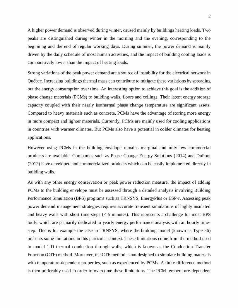
Figure 1-1 presents the prediction of the average power demand in Québec in January and July
2007 performed by Hydro-Québec in 2006. Clear seasonal and hourly differences are observed.
Figure 1-1: Prediction of the average hourly power demand in the province of Québec in January
and July 2007 (Hydro-Québec, 2006)
2
A higher power demand is observed during winter, caused mainly by buildings heating loads. Two
peaks are distinguished during winter in the morning and the evening, corresponding to the
beginning and the end of regular working days. During summer, the power demand is mainly
driven by the daily schedule of most human activities, and the impact of building cooling loads is
comparatively lower than the impact of heating loads.
Strong variations of the peak power demand are a source of instability for the electrical network in
Québec. Increasing buildings thermal mass can contribute to mitigate these variations by spreading
out the energy consumption over time. An interesting option to achieve this goal is the addition of
phase change materials (PCMs) to building walls, floors and ceilings. Their latent energy storage
capacity coupled with their nearly isothermal phase change temperature are significant assets.
Compared to heavy materials such as concrete, PCMs have the advantage of storing more energy
in more compact and lighter materials. Currently, PCMs are mainly used for cooling applications
in countries with warmer climates. But PCMs also have a potential in colder climates for heating
applications.
However using PCMs in the building envelope remains marginal and only few commercial
products are available. Companies such as Phase Change Energy Solutions (2014) and DuPont
(2012) have developed and commercialized products which can be easily implemented directly in
building walls.
As with any other energy conservation or peak power reduction measure, the impact of adding
PCMs to the building envelope must be assessed through a detailed analysis involving Building
Performance Simulation (BPS) programs such as TRNSYS, EnergyPlus or ESP-r. Assessing peak
power demand management strategies requires accurate transient simulations of highly insulated
and heavy walls with short time-steps (< 5 minutes). This represents a challenge for most BPS
tools, which are primarily dedicated to yearly energy performance analysis with an hourly time-
step. This is for example the case in TRNSYS, where the building model (known as Type 56)
presents some limitations in this particular context. These limitations come from the method used
to model 1-D thermal conduction through walls, which is known as the Conduction Transfer
Function (CTF) method. Moreover, the CTF method is not designed to simulate building materials
with temperature-dependent properties, such as experienced by PCMs. A finite-difference method
is then preferably used in order to overcome these limitations. The PCM temperature-dependent
3
thermal capacity is generally modeled with enthalpy-temperature or specific-heat-temperature
curves. Unfortunately, most models do not include the whole complexity of PCMs thermal
behavior. A differentiation between heating and cooling processes is rarely modeled while
subcooling is almost never taken into account.
Modeling a PCM requires to know its thermophysical properties, i.e. density, thermal conductivity
and capacity. Manufacturers document most of the time these main properties. However, these data
are generally incomplete or not representative. For example, the definition of the thermal
conductivity is often given with only one value, while PCM thermal conductivity is actually
variable, depending on its temperature and state (liquid or solid). Likewise, the PCM thermal
capacity values provided by manufacturers are often incomplete and do not always represent the
actual final product. Few data sheets provided by manufacturers include enthalpy-temperature or
specific heat-temperature curves for heating and cooling processes. If provided, these curves are
most often obtained using Differential Scanning Calorimetry (DSC) tests. This method uses small
samples (a few milligrams) and imposes high heat fluxes to the sample, which is not representative
of PCMs implemented in building walls (large quantity of PCMs, relatively low heat fluxes and
temperature variations).
The three main objectives of this thesis result from the above-mentioned issues and two of them
are composed of several more specific goals:
- Improvement of the CTF method in TRNSYS to allow accurate low-time-step simulations of
buildings with highly resistive and heavy walls.
- Accurate and representative characterization of a selected PCM:
o Evaluation of the density and thermal conductivity through experimentations.
o Evaluation of the temperature-dependent thermal capacity based on inverse methodology
and analysis of the impacts of different configurations (PCM samples of a few grams or
walls equipped with PCMs) and varying heating / cooling rates on this property.
o In the case of a PCM with 2 enthalpy-temperature curves (heating and cooling):
identification of the PCM thermal behavior when phase change is interrupted.
- Accurate modeling of a wall with PCMs, considering all aspects of the PCM thermal behavior
complexity:

4
o Development of a model of wall including PCM(s) or layer(s) with temperature-dependent
properties.
o Numerical validation of the developed model through a comparison with reference models
for several wall test cases.
o Experimental validation of the developed model using experimental data from a full-scale
test-bench.
Preliminary notes and clarifications:
a) In the present thesis, it is indicated that DSC tests should not be used to determine the 𝐻(𝑇)
curves because they are not representative of the way how PCMs are used in the building
envelope. DSC tests are intended to obtain the latent heat and the melting temperature of a
PCM, but they are often used by practitioners and researchers in building sciences to obtain the
𝐻(𝑇) curve of a PCM. The work in this thesis shows that the 𝐻(𝑇) curves obtained through
this method are not applicable to the PCM encapsulation techniques and thermal solicitations
typically found in buildings. Rather than the DSC tests, it is the extrapolated 𝐻(𝑇) curves that
cannot be used.
b) In this thesis, the term “subcooling” is used to denote the phenomenon observed when a PCM
is cooled below its solidification temperature, which is followed by a sudden temperature
increase (after a perturbation) leading to solidification. This phenomenon is more properly
denoted by supercooling.
c) The experimental results presented in this thesis aim to show that phase change differs
depending on the experimental conditions, especially the phase change temperature range
during melting and solidification. In this thesis, phase change temperature range denotes the
temperature “plateau” observed in graphs showing PCM temperature evolutions and defined
between two temperatures, often interpreted as the “onset” and “offset” of fusion or
solidification. Below the lower temperature, the PCM is assumed solid. On the other hand, the
PCM is supposed liquid if the measured temperature is beyond the upper temperature. These
interpretations are often found in the scientific literature but may not be strictly accurate from
the chemical point of view.

5
d) Temperature measurements during all experimentations presented in this thesis are performed
using T-type thermocouples, having a measurement uncertainty of ± 0.5 °C.

6
CHAPTER 2 LITERATURE REVIEW
This literature review first discusses heat transfer modeling in Building Performance Simulation
(BPS) tools (section 2.1), focusing on transient conduction through walls (section 2.2). The
modeling of transient conduction heat transfer with the presence of PCMs is then presented in
section 2.3.
2.1 Heat transfer modeling in buildings
Most BPS programs such as TRNSYS (Klein et al., 2012), EnergyPlus (Crawley et al., 2001) and
ESP-r (Energy Systems Research Unit, 1998) are based on the heat balance methodology for
modeling the whole heat transfer in buildings. This method is illustrated in Figure 2-1 (ASHRAE,
2013).
Figure 2-1: Heat balance method (ASHRAE, 2013)
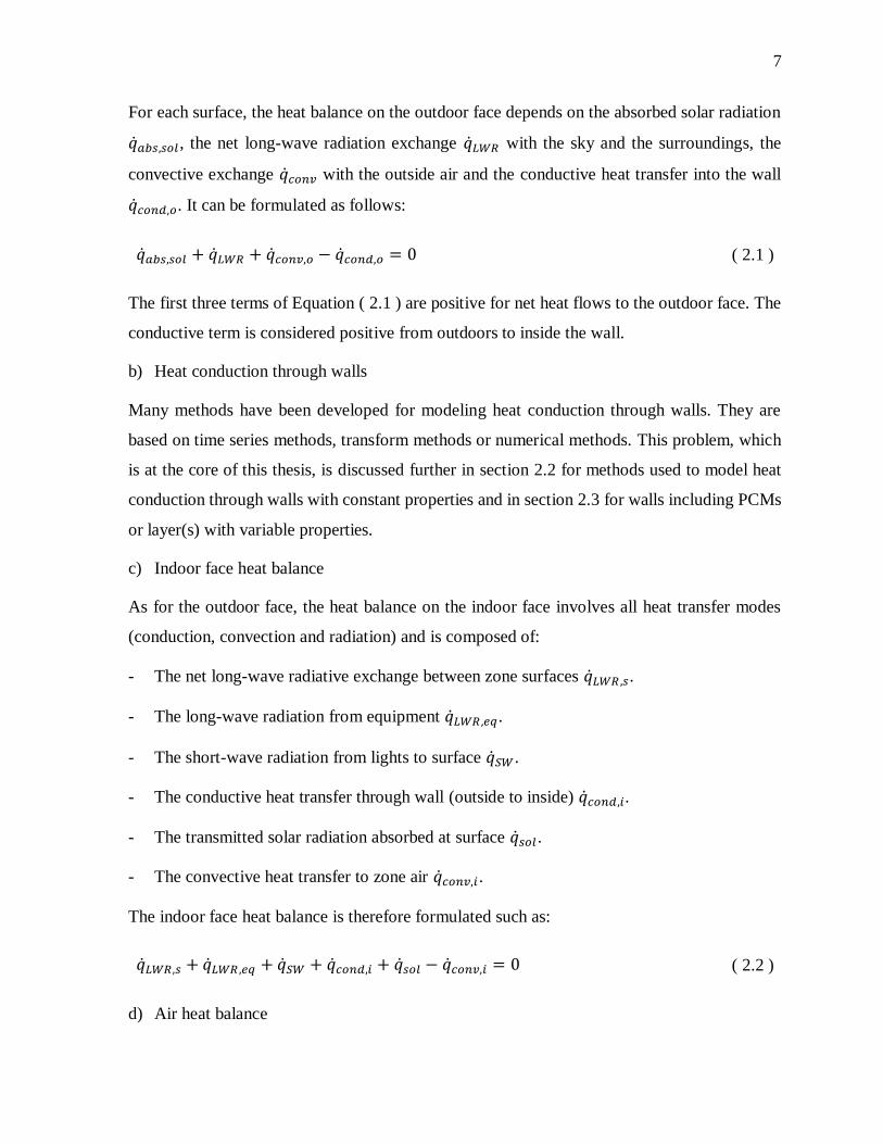
The heat balance method can be viewed as four distinct processes (as suggested in Figure 2-1):
a) Outdoor face heat balance
7
For each surface, the heat balance on the outdoor face depends on the absorbed solar radiation
��𝑎𝑏𝑠,𝑠𝑜𝑙, the net long-wave radiation exchange ��𝐿𝑊𝑅 with the sky and the surroundings, the
convective exchange ��𝑐𝑜𝑛𝑣 with the outside air and the conductive heat transfer into the wall
��𝑐𝑜𝑛𝑑,𝑜. It can be formulated as follows:
��𝑎𝑏𝑠,𝑠𝑜𝑙 + ��𝐿𝑊𝑅 + ��𝑐𝑜𝑛𝑣,𝑜 − ��𝑐𝑜𝑛𝑑,𝑜 = 0 ( 2.1 )
The first three terms of Equation ( 2.1 ) are positive for net heat flows to the outdoor face. The
conductive term is considered positive from outdoors to inside the wall.
b) Heat conduction through walls
Many methods have been developed for modeling heat conduction through walls. They are
based on time series methods, transform methods or numerical methods. This problem, which
is at the core of this thesis, is discussed further in section 2.2 for methods used to model heat
conduction through walls with constant properties and in section 2.3 for walls including PCMs
or layer(s) with variable properties.
c) Indoor face heat balance
As for the outdoor face, the heat balance on the indoor face involves all heat transfer modes
(conduction, convection and radiation) and is composed of:
- The net long-wave radiative exchange between zone surfaces ��𝐿𝑊𝑅,𝑠.
- The long-wave radiation from equipment ��𝐿𝑊𝑅,𝑒𝑞.
- The short-wave radiation from lights to surface ��𝑆𝑊.
- The conductive heat transfer through wall (outside to inside) ��𝑐𝑜𝑛𝑑,𝑖.
- The transmitted solar radiation absorbed at surface ��𝑠𝑜𝑙.
- The convective heat transfer to zone air ��𝑐𝑜𝑛𝑣,𝑖.
The indoor face heat balance is therefore formulated such as:
��𝐿𝑊𝑅,𝑠 + ��𝐿𝑊𝑅,𝑒𝑞 + ��𝑆𝑊 + ��𝑐𝑜𝑛𝑑,𝑖 + ��𝑠𝑜𝑙 − ��𝑐𝑜𝑛𝑣,𝑖 = 0 ( 2.2 )
d) Air heat balance

8
The last balance to be performed is on the zone air. It is formulated as follows:
��𝐼𝑉 + ��𝐶𝐸 + ��𝑠𝑦𝑠 + ��𝑐𝑜𝑛𝑣,𝑖 = 0 ( 2.3 )
Where:
- ��𝐼𝑉 is the sensible load caused by infiltration and ventilation.
- ��𝐶𝐸 is the convective gains of internal loads (e.g. heat released by occupants).
- ��𝑠𝑦𝑠 is the heat transfer to/from HVAC system.
- ��𝑐𝑜𝑛𝑣,𝑖 is the convection from all surfaces.
The three first elements a) to c) are duplicated for each surface while the last (air heat balance) is
carried out for each air node.
2.2 1-D conduction heat transfer modeling through walls
Transient heat conduction in BPS programs is mainly modeled using two methods. First, the
Conduction Transfer Function (CTF) method is an analytical method and is for example used in
TRNSYS and EnergyPlus. Secondly, finite-difference methods are numerical methods and are used
in ESP-r and optionally in EnergyPlus. Prior to reviewing these methods, a brief reminder on the
Fourier law and two important dimensionless numbers is presented.
2.2.1 Fourier law and dimensionless numbers
Conduction heat transfer was experimentally defined by Fourier (1822), who formulated the
following relationship:
𝑑𝑄
𝑑𝑡= −𝑘 𝐴
𝑑𝑇
𝑑𝑥 ( 2.4 )
Equation ( 2.4 ) indicates that the heat flow is proportional to the heat exchange surface 𝐴, the
thermal conductivity 𝑘 and the temperature gradient between 2 points.
In order to characterize transient conduction problems, two dimensionless numbers are of interest:
Fourier and Biot numbers.

9
Named after Fourier, this number Fo is the ratio of the heat conduction rate to the rate of thermal
energy storage in a solid (Bergman, Lavine, Incropera, & Dewitt, 2011). It is sometimes defined
as dimensionless time. It is formulated as follows:
Fo =𝛼 ∆𝑡
𝐿𝑐2 ( 2.5 )
Where 𝐿𝑐 is the characteristic length and the thermal diffusivity 𝛼 depends on the thermal
conductivity 𝑘, on the density 𝜌 and on the specific heat 𝐶𝑝 and is computed such as:
𝛼 =𝑘
𝜌 𝐶𝑝 ( 2.6 )
Physically a lower Fourier number means a lower heat transmission rate. It also means that the
thermal mass increases.
The second dimensionless number is the Biot number. It is defined as the ratio of the internal
thermal resistance of a solid to the boundary layer thermal resistance (Bergman et al., 2011). This
number is mathematically expressed as follows:
Bi =ℎ 𝐿𝑐𝑘
( 2.7 )
Where ℎ is the convective heat transfer coefficient.
A Biot number with a value higher than 1 means that the heat transmission rate is lower inside the
material than at its surface. It also indicates a significant temperature gradient inside the material.
This temperature gradient is theoretically assumed negligible if the Biot number is equal to or lower
than 0.1. Computing the Biot number is also a way to validate the conformity of using a lumped
capacitance model.
2.2.2 Conduction transfer function method
CTF method is used in BPS programs like TRNSYS to model 1-D transient heat conduction
through building walls with constant thermophysical properties. This method was primarily
developed by Stephenson and Mitalas (1971) and consists in computing the Conduction Transfer
Functions by solving the heat conduction equation with the Laplace and Z transforms theory. Later,

10
Mitalas and Arseneault (1972) developed an algorithm to compute the CTF coefficients, based
upon the method of Stephenson and Mitalas.
Figure 2-2: CTF method
Conduction Transfer Functions solve linear time invariant (LTI) systems from time series
composed of current and past inputs and past outputs. In TRNSYS, the CTF method computes the
inside and outside surface heat flows ��𝑠𝑖 and ��𝑠𝑜 from current and past values of the inside and
outside surface temperatures 𝑇𝑠𝑖 and 𝑇𝑠𝑜 and from the past outputs values (��𝑠𝑖 and ��𝑠𝑜) (Figure
2-2):
��𝑠𝑖,𝑡 =∑𝑏𝑡−𝑖∆𝑡𝑏 𝑇𝑠𝑜,𝑡−𝑖∆𝑡𝑏
𝑛𝑏
𝑖=0
−∑𝑐𝑡−𝑖∆𝑡𝑏 𝑇𝑠𝑖,𝑡−𝑖∆𝑡𝑏
𝑛𝑐
𝑖=0
−∑𝑑𝑡−𝑖∆𝑡𝑏 ��𝑠𝑖,𝑡−𝑖∆𝑡𝑏
𝑛𝑑
𝑖=1
( 2.8 )
��𝑠𝑜,𝑡 =∑𝑎𝑡−𝑖∆𝑡𝑏 𝑇𝑠𝑜,𝑡−𝑖∆𝑡𝑏
𝑛𝑎
𝑖=0
−∑𝑏𝑡−𝑖∆𝑡𝑏 𝑇𝑠𝑖,𝑡−𝑖∆𝑡𝑏
𝑛𝑏
𝑖=0
−∑𝑑𝑡−𝑖∆𝑡𝑏 ��𝑠𝑜,𝑡−𝑖∆𝑡𝑏
𝑛𝑑
𝑖=1
( 2.9 )
Where the coefficients 𝑎, 𝑏, 𝑐 and 𝑑 must meet the following requirement:
∑ 𝑎𝑡−𝑖∆𝑡𝑏𝑛𝑎𝑖=0
∑ 𝑑𝑡−𝑖∆𝑡𝑏𝑛𝑑𝑖=0
=∑ 𝑏𝑡−𝑖∆𝑡𝑏𝑛𝑏𝑖=0
∑ 𝑑𝑡−𝑖∆𝑡𝑏𝑛𝑑𝑖=0
=∑ 𝑐𝑡−𝑖∆𝑡𝑏𝑛𝑐𝑖=0
∑ 𝑑𝑡−𝑖∆𝑡𝑏𝑛𝑑𝑖=0
= 𝑈 ( 2.10 )
∆𝑡𝑏 is named the timebase and is the CTF time-step. It must be equal to or an integer multiple of
the simulation time-step. If 𝑖 equals 0 in Equations ( 2.8 ) to ( 2.10 ), it means the current time-step.
If 𝑖 equals 1, it then means the previous time-step. And so on until it reaches the number of
coefficients.
11
Equations ( 2.8 ) and ( 2.9 ) depend on the current surface temperatures 𝑇𝑠𝑖 and 𝑇𝑠𝑜, which are
unknown. Surface temperatures depend on net convective and radiative heat gains with the
surroundings but also on the heat conduction through the wall. Surface heat balance is solved using
an iterative procedure, as explained and suggested by Mitalas (1968).
Coefficients 𝑎, 𝑏, 𝑐 and 𝑑 characterize the thermal behavior of a wall and can be generated using
several methods, which were for example compared by Li et al. (2009). The mainly used two
methods are the Direct Root Finding (DRF) and State-Space (SS) methods. The first was developed
by Mitalas, Stephenson and Arseneault (Mitalas & Arseneault, 1972; Stephenson & Mitalas, 1971)
and is used in TRNSYS. On the other hand, the latter was developed by Ceylan, Myers and Seem
(Ceylan & Myers, 1980; Seem, 1987) and is implemented in EnergyPlus.
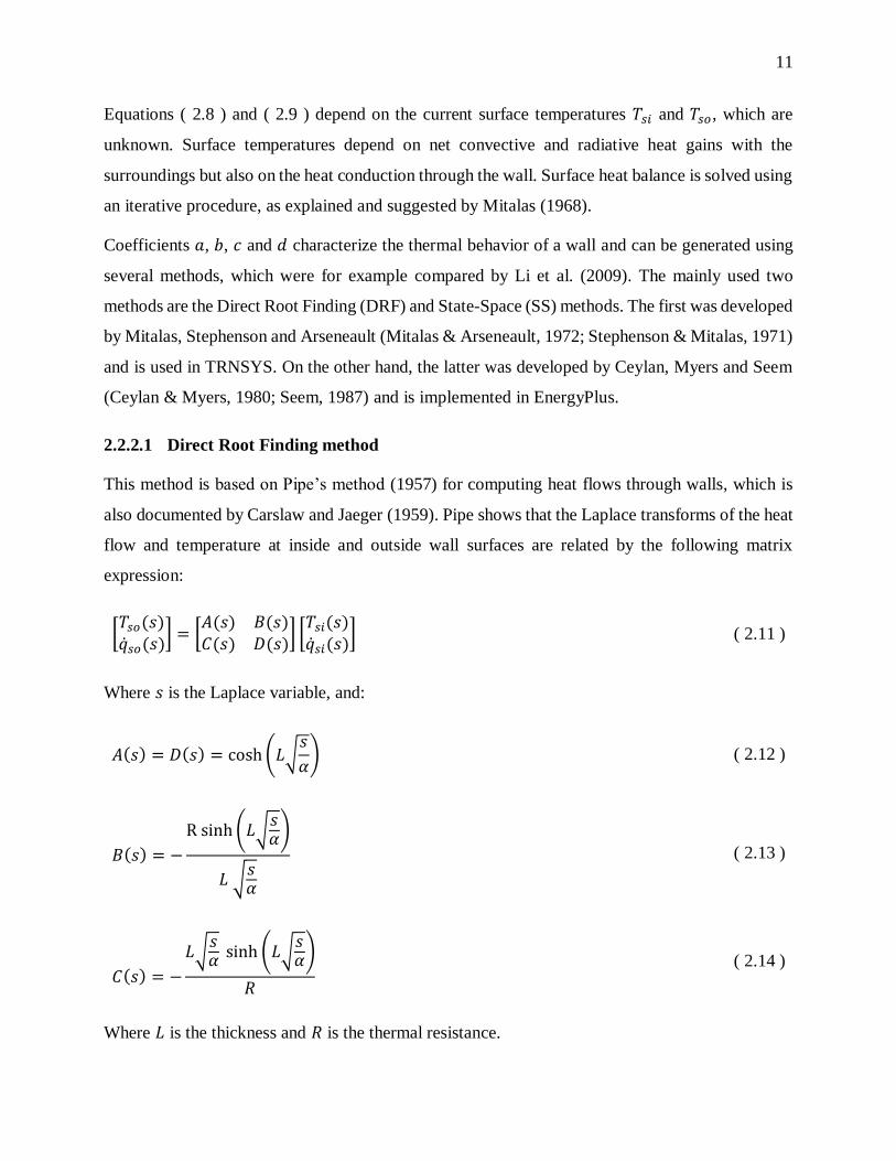
2.2.2.1 Direct Root Finding method
This method is based on Pipe’s method (1957) for computing heat flows through walls, which is
also documented by Carslaw and Jaeger (1959). Pipe shows that the Laplace transforms of the heat
flow and temperature at inside and outside wall surfaces are related by the following matrix
expression:
[𝑇𝑠𝑜(𝑠)��𝑠𝑜(𝑠)
] = [𝐴(𝑠) 𝐵(𝑠)𝐶(𝑠) 𝐷(𝑠)
] [𝑇𝑠𝑖(𝑠)��𝑠𝑖(𝑠)
] ( 2.11 )
Where 𝑠 is the Laplace variable, and:
𝐴(𝑠) = 𝐷(𝑠) = cosh (𝐿√𝑠
𝛼) ( 2.12 )
𝐵(𝑠) = −
R sinh (𝐿√𝑠𝛼)
𝐿 √𝑠𝛼
( 2.13 )
𝐶(𝑠) = −
𝐿√𝑠𝛼 sinh (𝐿√
𝑠𝛼)
𝑅
( 2.14 )
Where 𝐿 is the thickness and 𝑅 is the thermal resistance.
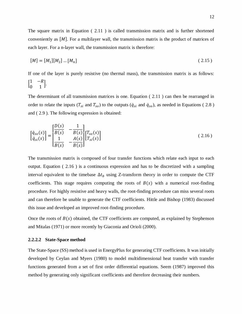
12
The square matrix in Equation ( 2.11 ) is called transmission matrix and is further shortened
conveniently as [𝑀]. For a multilayer wall, the transmission matrix is the product of matrices of
each layer. For a n-layer wall, the transmission matrix is therefore:
[𝑀] = [𝑀1][𝑀2] … [𝑀𝑛] ( 2.15 )
If one of the layer is purely resistive (no thermal mass), the transmission matrix is as follows:
[1 −𝑅0 1
].
The determinant of all transmission matrices is one. Equation ( 2.11 ) can then be rearranged in
order to relate the inputs (𝑇𝑠𝑖 and 𝑇𝑠𝑜) to the outputs (��𝑠𝑖 and ��𝑠𝑜), as needed in Equations ( 2.8 )
and ( 2.9 ). The following expression is obtained:
[��𝑠𝑜(𝑠)��𝑠𝑖(𝑠)
] =
[ 𝐷(𝑠)
𝐵(𝑠)−
1
𝐵(𝑠)
1
𝐵(𝑠)−𝐴(𝑠)
𝐵(𝑠)]
[𝑇𝑠𝑜(𝑠)𝑇𝑠𝑖(𝑠)
] ( 2.16 )
The transmission matrix is composed of four transfer functions which relate each input to each
output. Equation ( 2.16 ) is a continuous expression and has to be discretized with a sampling
interval equivalent to the timebase ∆𝑡𝑏 using Z-transform theory in order to compute the CTF
coefficients. This stage requires computing the roots of 𝐵(𝑠) with a numerical root-finding
procedure. For highly resistive and heavy walls, the root-finding procedure can miss several roots
and can therefore be unable to generate the CTF coefficients. Hittle and Bishop (1983) discussed
this issue and developed an improved root-finding procedure.
Once the roots of 𝐵(𝑠) obtained, the CTF coefficients are computed, as explained by Stephenson
and Mitalas (1971) or more recently by Giaconia and Orioli (2000).
2.2.2.2 State-Space method
The State-Space (SS) method is used in EnergyPlus for generating CTF coefficients. It was initially
developed by Ceylan and Myers (1980) to model multidimensional heat transfer with transfer
functions generated from a set of first order differential equations. Seem (1987) improved this
method by generating only significant coefficients and therefore decreasing their numbers.

13
Myers (1971) showed that a heat transfer problem can be modeled with a state-space
representation, using finite-difference method to spatially discretize the problem. Heat transfer
problems can then be presented such as LTI systems with 𝑛𝑠 states, 𝑛𝑖 inputs and 𝑛𝑜 outputs:
𝑑 [𝑇1…𝑇𝑛
]
𝑑𝑡= [𝐴] [
𝑇1…𝑇𝑛
] + [𝐵] [𝑇𝑖𝑇𝑜]
( 2.17 )
[��𝑖��𝑜] = [𝐶] [
𝑇1…𝑇𝑛
] + [𝐷] [𝑇𝑖𝑇𝑜] ( 2.18 )
Where 𝐴, 𝐵, 𝐶 and 𝐷 are matrices with constant coefficients. Their sizes are respectively (𝑛𝑠,𝑛𝑠),
(𝑛𝑠,𝑛𝑖), (𝑛𝑜,𝑛𝑠) and (𝑛𝑜,𝑛𝑖). Temperatures 𝑇𝑖 and 𝑇𝑜 are inputs. Heat flows ��𝑖 and ��𝑜 are outputs.
The vector including temperatures 𝑇1 to 𝑇𝑛 is the state vector.
Figure 2-3 presents a practical example of a homogeneous wall modeled with 2 nodes at the outside
and inside surfaces, using the electrical (Resistor – Capacitor) analogy.
Figure 2-3: 1-D two-node model of a wall
The following equations can be written for the example illustrated in Figure 2-3:
𝐶1𝑑𝑇1𝑑𝑡
= ℎ 𝐴 (𝑇𝑜 − 𝑇1) + 𝑈 𝐴 (𝑇2 − 𝑇1) ( 2.19 )
𝐶2𝑑𝑇2𝑑𝑡
= ℎ 𝐴 (𝑇𝑖 − 𝑇2) + 𝑈 𝐴 (𝑇1 − 𝑇2) ( 2.20 )
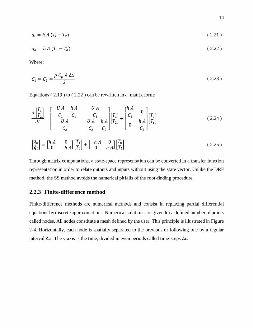
14
��𝑖 = ℎ 𝐴 (𝑇𝑖 − 𝑇2) ( 2.21 )
��𝑜 = ℎ 𝐴 (𝑇1 − 𝑇𝑜) ( 2.22 )
Where:
𝐶1 = 𝐶2 =𝜌 𝐶𝑝 𝐴 ∆𝑥
2 ( 2.23 )
Equations ( 2.19 ) to ( 2.22 ) can be rewritten in a matrix form:
𝑑 [𝑇1𝑇2]
𝑑𝑡=
[ −𝑈 𝐴
𝐶1−ℎ 𝐴
𝐶1
𝑈 𝐴
𝐶1𝑈 𝐴
𝐶2−𝑈 𝐴
𝐶2−ℎ 𝐴
𝐶2 ]
[𝑇1𝑇2] +
[ ℎ 𝐴
𝐶10
0ℎ 𝐴
𝐶2 ]
[𝑇𝑜𝑇𝑖] ( 2.24 )
[��𝑜��𝑖] = [ℎ 𝐴 0
0 −ℎ 𝐴] [𝑇1𝑇2] + [
−ℎ 𝐴 00 ℎ 𝐴
] [𝑇𝑜𝑇𝑖] ( 2.25 )
Through matrix computations, a state-space representation can be converted in a transfer function
representation in order to relate outputs and inputs without using the state vector. Unlike the DRF
method, the SS method avoids the numerical pitfalls of the root-finding procedure.
2.2.3 Finite-difference method
Finite-difference methods are numerical methods and consist in replacing partial differential
equations by discrete approximations. Numerical solutions are given for a defined number of points
called nodes. All nodes constitute a mesh defined by the user. This principle is illustrated in Figure
2-4. Horizontally, each node is spatially separated to the previous or following one by a regular
interval ∆𝑥. The y-axis is the time, divided in even periods called time-steps ∆𝑡.

15
Figure 2-4: 1-D finite-difference grid
The core idea of finite-difference methods is to replace derivatives by discrete approximations. For
example, the time derivative of the temperature of node 𝑛 can be approximated as follows:
𝑑𝑇𝑛𝑑𝑡
=𝑇𝑛𝑡+1 − 𝑇𝑛
𝑡
∆𝑡+ 𝒪(∆𝑡) ( 2.26 )
Where 𝒪(∆𝑡) is the truncation error caused by the approximation, which is proportional to the used
time-step ∆𝑡.
The 1-D heat equation is formulated in the following form:
𝑑𝑇
𝑑𝑡= 𝛼
𝑑2𝑇
𝑑𝑥2 ( 2.27 )
Equation ( 2.27 ) is composed of a first order time derivative and a second order space derivative.
When approximated, the accuracy of the numerical solution depends on the time-step ∆𝑡 and on
the space interval ∆𝑥. The more they approach zero, the more the computed solution approaches
the ideal solution and the more the model is time-consuming. The combination of nodes used to
compute the solution determines the type of finite-difference method. Numerical solutions to heat
transfer problems have been documented by several authors, such as Ames (1992), Cooper (1998),
Morton and Mayers (1994). Fletcher (1988) also discussed for some methods their implementation
in Fortran.

16
Prior to discussing further different finite-difference methods (explicit, implicit and Crank-
Nicolson), a brief review of methods for selecting the number of nodes to spatially discretize a wall
is presented.
2.2.3.1 Spatial discretization
The definition of a criteria in order to choose the number of nodes and the manner to distribute
them in multilayer walls in finite-difference models has been discussed by Waters and Wright
(1985) and in the engineering reference of EnergyPlus (2014).
For the number of nodes, both references have different approaches. Waters and Wright suggest to
compare each layer to the others. For each layer, a value called 𝛽 is computed as follows:
𝛽 =𝛼
𝐿2 ( 2.28 )
Where 𝛼 is the thermal diffusivity and 𝐿 is the thickness. Higher 𝛽 values result from lower thermal
resistances and capacitances, and a lower number of nodes is then attributed to the layer. The
number of nodes 𝑛 per layer is calculated such as:
𝑛 = 𝑛𝑚𝑖𝑛√𝛽𝑚𝑎𝑥𝛽𝑖
( 2.29 )
Where 𝑛𝑚𝑖𝑛 is the minimum number of nodes, 𝛽𝑚𝑎𝑥 is the maximum 𝛽 value among all layers and
𝛽𝑖 is the 𝛽 value of the layer for which the number of nodes is computed. The layer with the highest
𝛽 value (i.e. 𝛽𝑚𝑎𝑥) obtains the minimum number of nodes.
On the other hand, the method implemented in EnergyPlus is based on the Fourier number,
expressed through its inverse (𝐶𝑑 = 1/𝐹𝑜), to choose the number of nodes per layer. A space
interval between 2 nodes is computed for each layer such as:
∆𝑥 = √𝐶𝑑 𝛼 ∆𝑡 ( 2.30 )
In EnergyPlus, 𝐶𝑑 is fixed at 3 by default, which corresponds to a Fourier number of 1
3, i.e. a value
which satisfies the stability condition of the forward time and central space (FTCS) finite-

17
difference method (Bergman et al., 2011). Unlike the method proposed by Waters and Wright, this
method takes into account the time-step ∆𝑡.
Both methods distribute the nodes using the same methodology. They locate nodes on the limits of
boundary conditions, on each layer interface and inside each layer. Nodes on the limits of boundary
conditions and on each layer interface are considered as half-nodes while nodes inside each layer
are considered as whole nodes. For resistive layers, only one node is needed at the interface
between the previous layer and the resistive layer.
2.2.3.2 Explicit method
The explicit method uses current values (time 𝑡) to compute the future value for node 𝑛 (time 𝑡 +
1). Figure 2-5 illustrates this method, which is also called forward time and central space method.
Figure 2-5: Explicit scheme
As shown in (Recktenwald, 2011), the first order time derivative and the second order space
derivative in Equation ( 2.27 ) can be approximated as follows:
𝑑𝑇𝑛𝑑𝑡
=𝑇𝑛𝑡+1 − 𝑇𝑛
𝑡
∆𝑡+ 𝒪(∆𝑡) ( 2.31 )
𝑑2𝑇𝑛𝑑𝑥2
=𝑇𝑛−1𝑡 − 2𝑇𝑛
𝑡 + 𝑇𝑛+1𝑡
∆𝑥2+ 𝒪(∆𝑥2) ( 2.32 )
Where 𝒪 is the truncation error related to the approximations. This error depends on the time-step
∆𝑡 and on the square of the space interval ∆𝑥.
The terms of Equation ( 2.27 ) can be substituted by the approximations given in Equations ( 2.31 )
and ( 2.32 ):
18
𝑇𝑛𝑡+1 − 𝑇𝑛
𝑡
∆𝑡= 𝛼
𝑇𝑛−1𝑡 − 2𝑇𝑛
𝑡 + 𝑇𝑛+1𝑡
∆𝑥2 + 𝒪(∆𝑡) + 𝒪(∆𝑥2) ( 2.33 )
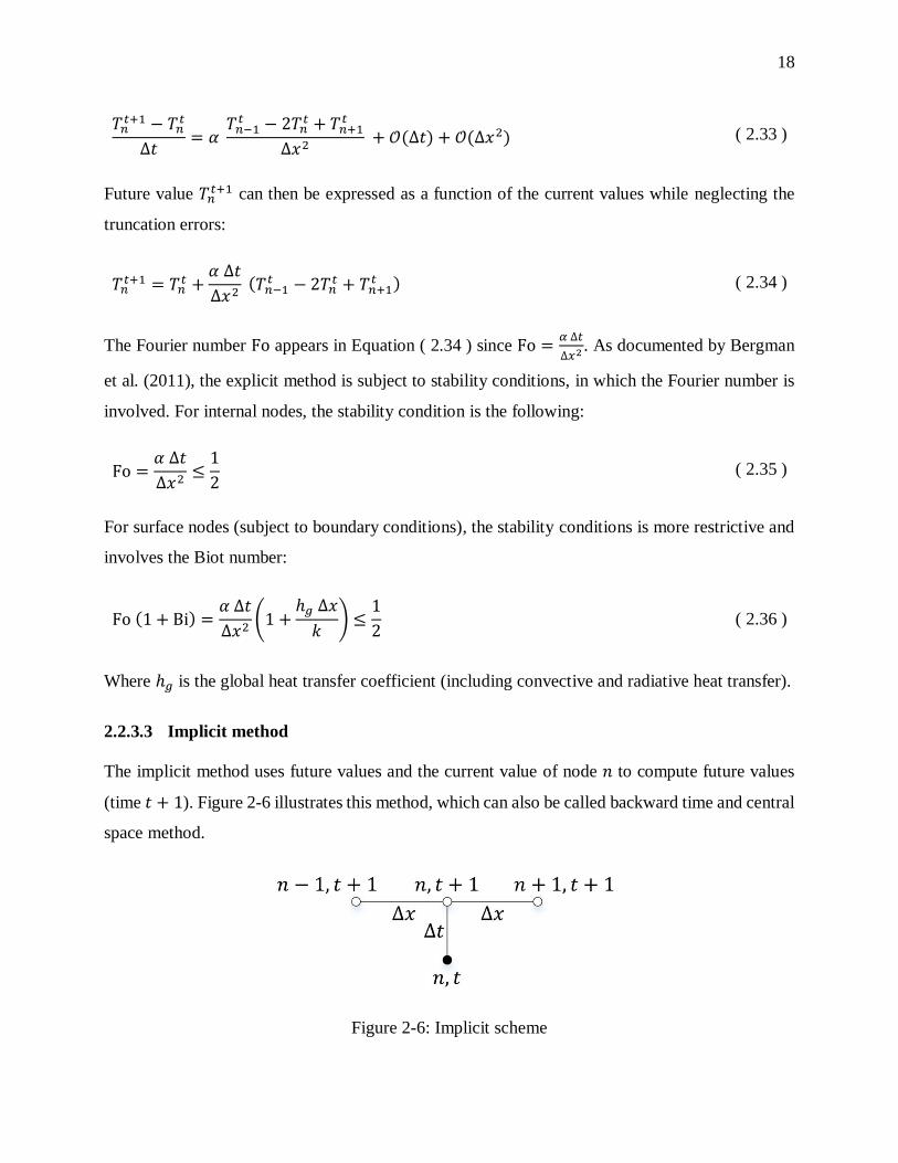
Future value 𝑇𝑛𝑡+1 can then be expressed as a function of the current values while neglecting the
truncation errors:
𝑇𝑛𝑡+1 = 𝑇𝑛
𝑡 +𝛼 ∆𝑡
∆𝑥2 (𝑇𝑛−1
𝑡 − 2𝑇𝑛𝑡 + 𝑇𝑛+1
𝑡 ) ( 2.34 )
The Fourier number Fo appears in Equation ( 2.34 ) since Fo =𝛼 ∆𝑡
∆𝑥2. As documented by Bergman
et al. (2011), the explicit method is subject to stability conditions, in which the Fourier number is
involved. For internal nodes, the stability condition is the following:
Fo =𝛼 ∆𝑡
∆𝑥2≤1
2 ( 2.35 )
For surface nodes (subject to boundary conditions), the stability conditions is more restrictive and
involves the Biot number:
Fo (1 + Bi) =𝛼 ∆𝑡
∆𝑥2(1 +
ℎ𝑔 ∆𝑥
𝑘) ≤
1
2 ( 2.36 )
Where ℎ𝑔 is the global heat transfer coefficient (including convective and radiative heat transfer).
2.2.3.3 Implicit method
The implicit method uses future values and the current value of node 𝑛 to compute future values
(time 𝑡 + 1). Figure 2-6 illustrates this method, which can also be called backward time and central
space method.
Figure 2-6: Implicit scheme
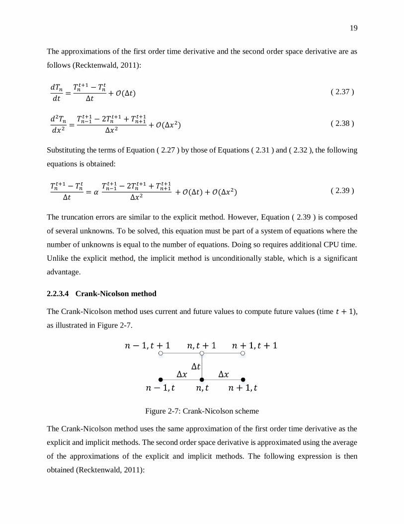
19
The approximations of the first order time derivative and the second order space derivative are as
follows (Recktenwald, 2011):
𝑑𝑇𝑛𝑑𝑡
=𝑇𝑛𝑡+1 − 𝑇𝑛
𝑡
∆𝑡+ 𝒪(∆𝑡) ( 2.37 )
𝑑2𝑇𝑛𝑑𝑥2
=𝑇𝑛−1𝑡+1 − 2𝑇𝑛
𝑡+1 + 𝑇𝑛+1𝑡+1
∆𝑥2+ 𝒪(∆𝑥2) ( 2.38 )
Substituting the terms of Equation ( 2.27 ) by those of Equations ( 2.31 ) and ( 2.32 ), the following
equations is obtained:
𝑇𝑛𝑡+1 − 𝑇𝑛
𝑡
∆𝑡= 𝛼
𝑇𝑛−1𝑡+1 − 2𝑇𝑛
𝑡+1 + 𝑇𝑛+1𝑡+1
∆𝑥2 + 𝒪(∆𝑡) + 𝒪(∆𝑥2) ( 2.39 )
The truncation errors are similar to the explicit method. However, Equation ( 2.39 ) is composed
of several unknowns. To be solved, this equation must be part of a system of equations where the
number of unknowns is equal to the number of equations. Doing so requires additional CPU time.
Unlike the explicit method, the implicit method is unconditionally stable, which is a significant
advantage.
2.2.3.4 Crank-Nicolson method
The Crank-Nicolson method uses current and future values to compute future values (time 𝑡 + 1),
as illustrated in Figure 2-7.
Figure 2-7: Crank-Nicolson scheme
The Crank-Nicolson method uses the same approximation of the first order time derivative as the
explicit and implicit methods. The second order space derivative is approximated using the average
of the approximations of the explicit and implicit methods. The following expression is then
obtained (Recktenwald, 2011):

20
𝑇𝑛𝑡+1 − 𝑇𝑛
𝑡
∆𝑡=𝛼
2 (𝑇𝑛−1𝑡+1 − 2𝑇𝑛
𝑡+1 + 𝑇𝑛+1𝑡+1
∆𝑥2+𝑇𝑛−1𝑡 − 2𝑇𝑛
𝑡 + 𝑇𝑛+1𝑡
∆𝑥2) + 𝒪(∆𝑡2)
+ 𝒪(∆𝑥2)
( 2.40 )
Like the implicit method, the discretized equation is composed of several unknowns and must be
solved as part of a system of equations. The Crank-Nicolson method is also considered
unconditionally stable. A significant advantage of this method is the better temporal truncation
error, which is proportional to the square of the time-step ∆𝑡 (instead of 𝒪(∆𝑡) for both explicit
and implicit schemes).
2.3 Conduction heat transfer modeling with PCM
Modeling conduction heat transfer through a PCM layer involves solving a set of non-linear
equations. This non-linearity comes from variable PCM properties, which depend on the PCM
temperature and state. The properties of interest are the thermal conductivity, the density and the
thermal capacity. All of them can be variable. A first discussed prerequisite is therefore the
determination of these properties. Then, 1-D modeling methods used to simulate the PCM thermal
behavior in building walls are reviewed. The last issue discussed in this section is modeling
approaches for specific thermal behaviors which can be observed when using PCMs.
2.3.1 PCM classification and thermophysical properties
As noted by Zalba et al. (2003), Sharma et al. (2009) and Baetens et al. (2010), PCMs are generally
classified in three categories, i.e. organics (e.g. paraffins, alcohols or fatty acids), inorganics (e.g.
salt hydrates) and eutectics. Eutectics are mixtures of organics and / or inorganics. According to
Sharma et al. (2009), inorganics have in general approximately twice more volumetric latent heat
storage capacity than organics. These review papers also present large lists of available PCMs with
their main properties.
These properties are measured using proven methods. The German Institute for Quality Assurance
and Certification (2013) have documented a list of possible methods used to measure the thermal
conductivity and capacity of PCMs.
The standard method for measuring PCM thermal conductivity is the hot-wire method (Alvarado,
Marín, Juárez, Calderón, & Ivanov, 2012; ASTM International, 2000). The hot-wire equipment is

21
composed of a data acquisition system and a needle which includes a heating wire and a
temperature probe. During measurements, the needle is immersed into a large PCM sample and is
considered as a linear heat source. The heat flow going across the sample is assumed radial. The
temperature evolution recorded by the probe defines the thermal conductivity. Lower measured
temperature increases lead to higher thermal conductivities.
In order to measure PCM temperature-dependent thermal capacity, the German Institute for Quality
Assurance and Certification (2013) suggests to use Differential Scanning Calorimetry (DSC) or
T-history methods. DSC technique was primarily developed by Watson et al. (1964). Its principle
is based on a comparative analysis of a PCM sample to a reference. The test consists in recording
the energy necessary over time flowing in (heating) or out (cooling) the sample and the reference
to maintain both at nearly the same temperature. The temperature-dependent specific heat is then
derived from the DSC results. Many authors point out several limitations when using DSC method.
As highlighted by Zhang et al. (1999) and Cheng et al. (2013), DSC tests are applied on very small
samples (1-10 mg). A careful sampling is consequently required to obtain a representative property.
A second limitation presented by Zhang et al. (1999) is the significant cost of DSC tests.
The T-history method is also based on a comparison between a PCM sample and a reference.
Initially, Zhang et al. (1999) proposed this method as an alternative to DSC tests. Unlike DSC
method, the sample size is higher (a few grams) and the test is less expensive to perform. During
T-history experimentations, the PCM sample and the reference (e.g. water) undergo a similar
cooling (or heating as suggested by Günther et al. (2006)). A comparison of temperature evolutions
between the PCM sample and the reference allows obtaining specific heat (solid and liquid) and
latent heat values of the PCM. Several authors have improved the T-history method, following
different approaches. Kravvaritis et al. (2010) proposed the “thermal delay method” (Figure 2-8
(a)), which consists in comparing the temperature variation of the PCM sample and the reference
during the same time range. On the other hand, Marín et al. (2003) suggested another approach
called “time delay method”. The goal is to compare the time durations passed on a defined
temperature range between the PCM sample and the reference (Figure 2-8 (b)). The temperature-
dependent specific heat is then obtained through these two approaches. An extensive review of the
T-history method is for example documented by Solé et al. (2013).

22
Figure 2-8: Two different approaches of T-history tests
Two limitations of the T-history method are discussed by Cheng et al. (2013). First, the sample
temperature must be considered uniform. Mathematically, it means that the Biot number must be
equal to or lower than 0.1 (Bergman et al., 2011). Second, a T-history method is not suited to
materials for which it is difficult to obtain a small uniform sample, e.g. PCM-concrete bricks as
studied by Cheng et al. (2013).
Other alternatives to measure the temperature-dependent specific-heat are also available. A method
based on a dynamic Heat Flow Meter Apparatus (“HFMA method”) was proposed by Kosny et al.
(2010). It can be applied to a large amount of PCM encapsulated in a plastic film, i.e. in conditions
closer to the actual use in buildings envelope. Coupling a detailed 3-D model of the plastic film
including PCM encapsulations and experimental data generated with the heat flow meter apparatus
allows obtaining the temperature-dependent specific heat of the PCM. Their presented results also
indicate that the latent heat calculated with the HFMA method is around 30 % lower than the value
obtained with the DSC test. This methodology is close to inverse modeling techniques. These latter
were already used to identify thermophysical properties of a material. Using experimental data and
a 1-D finite-element model coupled with an optimization algorithm based on least squares method,
Atchonouglo et al. (2008) identified the constant thermal capacity and conductivity of polymers.
Using the same methodology but with an optimization algorithm based on the conjugate gradient
method, Huang and Jan-Yuan (1995) determined simultaneously the temperature-dependent
thermal capacity and conductivity of a material. Cheng et al. (2013) also applied an inverse technic
for only obtaining the temperature-dependent specific-heat of PCM-concrete bricks. Several

23
optimization algorithms based on genetic algorithm, particle swarm optimization algorithm and
sequential quadratic programming method were coupled with a 1-D finite-difference model to
define this property and to determine the most effective algorithm. The results show that all
algorithms generate nearly the same optimized temperature-dependent specific-heat. They also
show that the sequential quadratic programming method is the most time-effective.
2.3.2 Modeling methods
Conduction heat transfer in PCMs is a moving boundary problem (Crank, 1987) or a Stefan
problem, named after the Slovene physicist who introduced this class of problem for ice formation.
An important dimensionless number named after Stefan is useful to analyze phase change
problems. It is defined as the ratio of sensible heat to latent heat and is formulated as:
St =𝐶𝑝 (𝑇𝑓𝑢𝑠𝑖𝑜𝑛 − 𝑇𝑠𝑦𝑠)
𝐿 ( 2.41 )
Moving boundary problem involves to deal with non-linear phenomena which change with time
and space. In the basic case of water solidification, this process involves the presence of liquid and
solid phases separated by a moving boundary which should be tracked. Few analytical solutions
exist for phase change problems and are among others formulated by Crank (1987), Alexiades and
Solomon (1992). Stefan was the first to propose analytical solutions to phase change problems,
which are documented, among others, by Hu and Argyropoulos (1996). Numerical methods are
nevertheless preferred since they are easily adapted to different cases. Numerical solutions are
classified into two main categories:
- Deforming grid or front-tracking methods (or strong solutions): the space grid is deformed
during calculations, depending on the position of the solidification / melting front. These
methods are for example described by Voller (1996). However they require time-
consuming calculations.
- Fixed grid methods (or weak solutions): the space grid remains fixed during calculations
and the solidification / melting front is tracked using an auxiliary function. These solutions
are widespread methods and some review papers document them (Al-Saadi & Zhai, 2013;
Voller, Swaminathan, & Thomas, 1990).

24
In the following sections, only fixed grid methods are discussed since they are the most suited for
1-D modeling of a wall with PCMs. Among these methods, two are mainly used in the literature:
the heat capacity and enthalpy methods, which are discussed below. Less often-used methods such
as the temperature transforming (Cao & Faghri, 1990) or heat source (for example reviewed by Al-
Saadi and Zhai (2013)) are not covered in this discussion.
2.3.2.1 Heat capacity method
The heat capacity method (Goodrich, 1978; Yao & Chait, 1993) consists in adapting the PCM
specific heat depending on its temperature and/or state. Until recently, two approaches, named the
apparent and effective heat capacity, were used to define this property. Their differences were in
particular discussed by Poirier (1986). For both terminologies, the apparent or effective specific-
heat combines sensible and latent heat. Today, both terminologies are interchangeably used.
The governing 1-D heat equation (Equation ( 2.27 )) can be rewritten as follows:
𝜌 𝐶𝑝(𝑇) 𝑑𝑇
𝑑𝑡=𝑑 (𝑘
𝑑𝑇𝑑𝑥)
𝑑𝑥
( 2.42 )
Where the specific heat 𝐶𝑝 is temperature-dependent (Figure 2-9 (a)). The core idea of this method
is then to approximate correctly this property for each location and time-step.
Figure 2-9: (a) Specific-heat – temperature and (b) enthalpy – temperature curves of a PCM with
a phase change temperature range [𝑇𝑠,𝑇𝑙]
Mathematically, the temperature-dependent specific-heat of a PCM with a solidification / melting
range can be computed such as (Voller, 1996):

25
𝐶𝑝 =
{
𝐶𝑝,𝑠, 𝑇 < 𝑇𝑠
𝐿
𝑇𝑙 − 𝑇𝑠, 𝑇𝑠 ≤ 𝑇 ≤ 𝑇𝑙
𝐶𝑝,𝑙, 𝑇 > 𝑇𝑙
( 2.43 )
Like the specific-heat, the thermal conductivity can be temperature-dependent and is determined
such as:
𝑘 = {
𝑘𝑠, 𝑇 < 𝑇𝑠(1 − 𝑙𝑓) 𝑘𝑠 + 𝑙𝑓 𝑘𝑙, 𝑇𝑠 ≤ 𝑇 ≤ 𝑇𝑙
𝑘𝑙 , 𝑇 > 𝑇𝑙
( 2.44 )
Where the liquid fraction 𝑙𝑓 is:
𝑙𝑓 =𝑇 − 𝑇𝑠𝑇𝑙 − 𝑇𝑠
𝑜𝑟 𝑙𝑓 =𝐻 −𝐻𝑠𝐻𝑙 − 𝐻𝑠
( 2.45 )
Equation ( 2.42 ) can be solved explicitly (Voller, 1996), using a forward time and central space
scheme such as (for node 𝑛):
𝑇𝑛𝑡+1 = 𝑇𝑛
𝑡 +𝛼 ∆𝑡
∆𝑥2 (𝑇𝑛−1
𝑡 − 2𝑇𝑛𝑡 + 𝑇𝑛+1
𝑡 ) ( 2.46 )
Where the thermal diffusivity 𝛼 depends on the temperature-dependent specific-heat and thermal
conductivity. The stability condition for this fully explicit scheme becomes:
𝑀𝑎𝑥(𝐹𝑜𝑠, 𝐹𝑜𝑙) = 𝑀𝑎𝑥 (𝛼𝑠 ∆𝑡
∆𝑥2,𝛼𝑙 ∆𝑡
∆𝑥2) ≤
1
2 ( 2.47 )
If a fully implicit or Crank-Nicolson scheme is applied, iterative calculations are required since the
specific-heat and thermal conductivity at time 𝑡 + 1 are unknown. Solving the equations system
requires using common linear solvers such as a Gauss-Seidel algorithm (Morgan, Lewis, &
Zienkiewicz, 1978) or a tridiagonal matrix algorithm (TDMA) (Pasupathy & Velraj, 2006). For
each iteration, the specific-heat must be updated such as proposed by Morgan et al. (1978):
𝐶𝑝 =∆𝐻
∆𝑇=𝐻𝑗+1 − 𝐻𝑗
𝑇𝑗+1 − 𝑇𝑗 ( 2.48 )

26
Where 𝐻 is the enthalpy and 𝑗 is the iteration level. This calculation is possible only if the enthalpy
– temperature curve is known (Figure 2-9 (b)). Unlike Morgan et al., Lemmon (1981) proposed to
approximate the specific-heat based on the space average (instead of the time average for Morgan
et al.).
Convergence is reached as soon as temperature variation between two iterations becomes
negligible. If the time-step is too large and / or the phase change temperature range is too small,
the phase change can be undetected and / or convergence issues can occur. Solutions to these
limitations were proposed in the literature (Gong & Mujumdar, 1997; Yao & Chait, 1993).
2.3.2.2 Enthalpy method
The governing 1-D heat equation (Equation ( 2.27 )) can be formulated using an enthalpy term
including sensible and latent heat:
𝜌 𝑑𝐻
𝑑𝑡=𝑑 (𝑘
𝑑𝑇𝑑𝑥)
𝑑𝑥
( 2.49 )
As suggested by Klimes et al. (2012), Equation ( 2.49 ) can be solved with an explicit finite-
difference method (for node 𝑛):
𝐻𝑛𝑡+1 = 𝐻𝑛
𝑡 +𝑘 ∆𝑡
𝜌 ∆𝑥2 (𝑇𝑛−1
𝑡 − 2𝑇𝑛𝑡 + 𝑇𝑛+1
𝑡 ) ( 2.50 )
The temperature values 𝑇𝑡+1 can then be calculated using the enthalpy – temperature curve (as
illustrated in Figure 2-9 (b)). The same stability condition as formulated in Equation ( 2.47 ) is
required.
If a fully implicit method is used, the future enthalpy 𝐻𝑛𝑡+1 of node 𝑛 depends on future
temperatures 𝑇𝑛−1𝑡+1, 𝑇𝑛
𝑡+1 and 𝑇𝑛+1𝑡+1 such as:
𝐻𝑛𝑡+1 = 𝐻𝑛
𝑡 +𝑘 ∆𝑡
𝜌 ∆𝑥2 (𝑇𝑛−1
𝑡+1 − 2𝑇𝑛𝑡+1 + 𝑇𝑛+1
𝑡+1) ( 2.51 )
The equations system (for all nodes) have therefore more unknowns than equations, which make
the resolution impossible.

27
The most used approach to solve Equation ( 2.51 ) consists in linearizing the enthalpy term 𝐻𝑛𝑡+1
using a technique proposed by Patankar (1980). At the iterative level, this term can be written as
follows:
𝐻𝑛𝑡+1,𝑗+1
= 𝐻𝑛𝑡+1,𝑗
+ 𝐶𝑝(𝑇)𝑡+1,𝑗(𝑇𝑛
𝑡+1,𝑗+1− 𝑇𝑛
𝑡+1,𝑗) ( 2.52 )
Equation ( 2.52 ) is substituted into Equation ( 2.51 ), which yields the following linear discretized
equation:
−𝑘 ∆𝑡
𝜌 ∆𝑥2 𝑇𝑛−1
𝑡+1,𝑗+1+ (𝐶𝑝(𝑇)
𝑡+1,𝑗 +2 𝑘 ∆𝑡
𝜌 ∆𝑥2) 𝑇𝑛
𝑡+1,𝑗+1−𝑘 ∆𝑡
𝜌 ∆𝑥2 𝑇𝑛+1
𝑡+1,𝑗+1
= 𝐻𝑛𝑡 −𝐻𝑛
𝑡+1,𝑗+ 𝐶𝑝(𝑇)
𝑡+1,𝑗𝑇𝑛𝑡+1,𝑗
( 2.53 )
Equation ( 2.53 ) can be formulated in a simplified matrix form:
[𝐴]𝑡+1,𝑗 × [𝑇]𝑡+1,𝑗+1 = [𝐵]𝑡+1,𝑗 ( 2.54 )
Equation ( 2.54 ) is then solved iteratively using a Gauss-Seidel algorithm (Shamsundar & Rooz,
1988; Shamsundar & Sparrow, 1975) or a tridiagonal matrix algorithm (TDMA) (Swaminathan &
Voller, 1993; Voller, 1996). Convergence is reached as soon as temperature variation between two
iterations become negligible.
In order to reduce computation time, a non-iterative method was also proposed by Pham (1985). It
consists in solving Equations ( 2.54 ) using a TDMA algorithm to obtain the temperature field.
Enthalpies are computed using Equation ( 2.52 ) and the temperature field is then corrected based
on the new enthalpies. Unfortunately, Voller (1996) showed that this method might not conserve
energy at every time-step.
2.3.2.3 Reported problems of iterative methods
Using implicit or semi-implicit finite-difference methods is advantageous since no restriction on
time-stepping is required. On the other hand, this kind of methods involves iterative calculations
when dealing with non-linear equations. Tavakoli and Davami (2007) showed that the product of
the number of time-steps by the number of iterations when using an implicit method might be
higher than the number of time-steps when using an explicit method. They took cases presented by

28
Swaminathan and Voller (1992) and compared their results generated with an implicit method to
results generated with a fully explicit method. The comparison indicated that explicit methods
might be more efficient than implicit methods since the number of iterations (including time-steps
and inner iterations) is less numerous for explicit schemes.
Another drawback is the difficulty to apply implicit methods for modeling PCMs with complex
thermal behaviors such as hysteresis and subcooling (presented in the following section). The
implicit methods presented previously were all adapted to cases with constant-temperature phase
change or phase change over a certain temperature range. None of them was applied on PCM with
subcooling and different thermal behavior during heating and cooling processes.
2.3.3 Specific PCM thermal behaviors
Most models do not take into account two specific PCM thermal behaviors: hysteresis and
subcooling. The first is highlighted by a different PCM thermal behavior during heating (melting)
and cooling (solidification) processes, as illustrated in Figure 2-10. Both melting and solidification
occur over different temperature ranges, which has an impact on the enthalpy – temperature curves.
Subcooling is experienced when the liquid state is cooled down below its assumed solidification
temperature (Figure 2-11). This is followed by a steep temperature increase caused by an abrupt
latent heat release, leading to solidification. Kuznik and Virgone (2009) and Günther et al. (2007)
suggest that the hysteresis and the subcooling can have a significant impact on PCM performance,
respectively. Günther et al. (2007) also present a manner to model subcooling in PCMs.
Figure 2-10: PCM hysteresis

29
Figure 2-11: PCM subcooling
The presence of hysteresis in a PCM requires to model the transition between heating and cooling
enthalpy – temperature curves during phase change. Three scenarios are documented in the
literature. Bony and Citherlet (2007) propose to switch between curves using a slope equivalent to
the specific-heat in the liquid or solid state (“wT” in Figure 2-12). Another option suggested by
Chandrasekharan et al. (2013) consists in staying on the same curve (“noT” in Figure 2-12). The
last scenario proposed by Rose et al. (2009) is applied in the BPS program BSim (Danish Building
Energy Institute, 2013) and consists in instantaneous switches between heating and cooling curves.
Figure 2-12: Possible behavior of a PCM cooled down after partial melting
2.3.4 Existing models of a wall with PCMs
Several models of a wall including PCM layer(s) are available in well-known BPS programs such
as TRNSYS, EnergyPlus and ESP-r. ESP-r and EnergyPlus possess a PCM model which is directly

30
implemented in the building model. ESP-r uses a PCM model based on the effective heat capacity
method and solved with a finite-difference method (Heim & Clarke, 2004). The thermal
conductivity can be defined for liquid and solid states. On the other hand, subcooling and hysteresis
cannot be modeled. However Geissler (2008) recently implemented in ESP-r a development
version of a subroutine based on the work of Hoffman (2006) allowing to model hysteresis.
EnergyPlus does use an enthalpy method coupled with an iterative finite-difference method using
a fully implicit or Crank-Nicolson (C-N) scheme (Pedersen, 2007). This model was validated in
multiple studies (Shrestha et al., 2011; Tabares-Velasco, Christensen, Bianchi, & Booten, 2012;
Tabares-Velasco, Christensen, & Bianchi, 2012). Like ESP-r, the model implemented in
EnergyPlus is unable to define subcooling and hysteresis while a temperature-dependent thermal
conductivity can be modeled. It should be noted that EnergyPlus used to model heat conduction
through walls only with the CTF method. Barbour and Hittle (2005) have studied the possibility to
adapt the CTF method to PCM modeling in a development version of EnergyPlus. They proposed
to generate multiple sets of CTF coefficients, depending on the PCM state and temperature. A
switching mechanism deals with the selection of the right sets of CTF coefficients during the
simulation. To our knowledge this method has never been implemented in the release version of
EnergyPlus.
In TRNSYS, different models exist to simulate PCM in building walls. These models are
encapsulated in components called “Types” and must be coupled with the multizone building
model, known as Type 56. The first PCM models developed in TRNSYS were simulated as an
active layer. This approach was used in Type 222 (Ibánez, Lázaro, Zalba, & Cabeza, 2005) and
Type 232 (Castell, Medrano, Castellón, & Cabeza, 2009). However, this methodology has been
superseded because it did not represent the actual physical phenomena. From this moment, all
TRNSYS PCM models were developed based on finite-difference (FD) methods. Type 1270
developed by TESS (Thermal Energy Systems Specialists, 2012) is a very simple PCM model
which considers a constant-temperature phase change and a spatially uniform temperature inside
the PCM layer. Multiple TRNSYS models such as Type 204 (Poulad, Fung, & Naylor, 2011), Type
260 (Kuznik, Virgone, & Johannes, 2010) and Type 399 (Dentel & Stephan, 2010a; Dentel &
Stephan, 2013) use the effective heat capacity method to model PCMs in walls. On the other hand,
the literature documents two models using an enthalpy method to simulate PCM in walls, i.e. Type
241 (Schranzhofer, Puschnig, Heinz, & Streicher, 2006) and Type 285 (Al-Saadi & Zhai, 2014).

31
Table 2-1 presents the most recent and documented PCM models for building walls available in
TRNSYS. It focuses on the main capabilities of each model. It also shows that:
- None of these models are able to model subcooling.
- Only one model (Type 399) is able to model PCM hysteresis.
- Temperature-dependent thermal conductivity can be defined in only one model.
Table 2-1: Most recent and documented PCM models for building walls in TRNSYS
Characteristics Type 1270 Type 285 Type 260 Type 399
PCM modeling
method
Constant-temperature
phase change
Enthalpy
method
Effective heat capacity
method
Numerical method Lumped capacitance
model
Iterative
implicit FD
method
Implicit
FD
method
Semi-implicit
FD method
(C-N)
Hysteresis No Yes
Subcooling No
Transition between
heating and
cooling curves
Not possible (one-curve model)
Instantaneous
switch between
𝐶𝑝(𝑇) curves.
Variable thermal
conductivity No Yes No

32
CHAPTER 3 OBJECTIVES AND THESIS ORGANIZATION
The literature review highlights current limitations when building walls including PCMs have to
be simulated in common BPS programs. No current BPS program is capable of modeling a wall
with PCMs including temperature-dependent thermal conductivity, hysteresis and subcooling. In
particular, TRNSYS is not adapted for this purpose since conduction heat transfer through walls is
modeled using the CTF method. This method is moreover not appropriate for low-time-step
simulations (< 5 minutes) of buildings with highly resistive and heavy walls.
The literature review also highlights the complexity of measuring PCM thermophysical properties,
and in particular the heat capacity. Measurement techniques can lead to different test results,
depending on the experimental conditions.
These limitations underlie the objectives formulated in the following section.
3.1 Objectives
The three main objectives of this thesis result from the above-mentioned issues and two of them
are composed of several more specific goals:
- Objective 1 – Improvement of the CTF method in TRNSYS to allow accurate low-time-
step simulations of buildings with highly resistive and heavy walls.
- Objective 2 – Accurate and representative characterization of thermophysical properties
of a selected PCM.
o Evaluation of the density and thermal conductivity through experimentations.
o Evaluation of the temperature-dependent thermal capacity based on inverse method and
analysis of the impacts of different configurations (PCM samples of a few grams or PCM-
equipped walls) and varying heating / cooling rates on this property.
o In the case of a PCM with 2 enthalpy-temperature curves (heating and cooling):
identification of the PCM thermal behavior when phase change is interrupted.
- Objective 3 – Development and validation of a 1-D finite-difference PCM wall model
implemented in TRNSYS.

33
o Development of a model of wall including PCM(s) (potentially with hysteresis and
subcooling) or layer(s) with temperature-dependent properties.
o Numerical validation of the developed model through a comparison with reference models
for several wall test cases.
o Experimental validation of the developed model using experimental data from a full-scale
test-bench.
3.2 Thesis organization
This thesis is composed of eleven chapters (including the introduction and the conclusion) and is
submitted as a thesis by articles. The literature review presented in Chapter 2 discusses the
modeling methods used to simulate conduction heat transfer through building walls without and
with PCMs. Chapter 3 presents the objectives and the organization of this thesis.
Chapter 4 presents the first article titled “Improved conduction transfer function coefficients
generation in TRNSYS multizone building model”. This paper discusses the limitations of the CTF
method implemented in TRNSYS and proposes a new algorithm based on the state-space method
for generating the CTF coefficients. This topic is also discussed in Chapter 5, highlighting the
benefit of coupling the CTF method with a finite-difference method. Both Chapter 4 and Chapter
5 address the first objective of this thesis dedicated to the improvement of the CTF method in
TRNSYS to allow short-time-step simulations of buildings with highly resistive and heavy walls
(required e.g. for simulating improved power demand management strategies).
Chapter 6 presents the second paper entitled “Influence of experimental conditions on measured
thermal properties used to model phase change materials” and published in Building Simulation:
An International Journal. This chapter focuses on the definition of the PCM temperature-dependent
heat capacity. Experimentations with PCM samples are performed and processed using an inverse
method in order to obtain 𝐶𝑝(𝑇) and 𝐻(𝑇) curves for both heating and cooling processes. The
density and thermal conductivity of the tested PCM are defined through additional
experimentations presented in Appendices A and B. Experimentations with PCMs included in
building walls are also presented. Since the PCM layer is also composed of air and plastic film,
this layer must be considered as an equivalent layer. 𝐶𝑝(𝑇) and 𝐻(𝑇) curves of this equivalent
layer are computed using an inverse method and the influence of the heating / cooling rates on the
34
𝐻(𝑇) curves are studied. The equivalent thermal conductivity is determined using THERM
(Lawrence Berkeley National Laboratory, 2013), as explained in Appendix C. Chapter 7
complements Chapter 6 by identifying the PCM thermal behavior when phase change is
interrupted. Both Chapter 6 and Chapter 7 address the second objective of this thesis, i.e. the
definition of thermophysical properties of the tested PCM.
Chapter 8 presents the fourth article entitled “Modeling of a wall with phase change materials.
Part I: Development and numerical validation”. This chapter describes in details a newly developed
PCM wall 1-D model based on an explicit finite-difference method and coupled with an enthalpy
method for PCM modeling. This model is named Type 3258 and is able to simulate a wall including
PCMs with temperature-dependent thermal conductivity, hysteresis and subcooling. A numerical
validation of the presented model is performed using wall test cases proposed by the International
Energy Agency. Part II of this paper (Chapter 9) completes this topic with an experimental
validation and with a discussion about the coupling methods used to link the multizone building
model to the PCM wall model in TRNSYS. The developed model (Type 3258) is also described in
details in Appendix D. Both Chapter 8 and Chapter 9 address the third objective of this thesis about
the development and validation of a new PCM wall model able to simulate PCMs with temperature-
dependent thermal conductivities, hysteresis and subcooling.
A general discussion presented in Chapter 10 highlights the main contributions of this thesis while
the conclusion and recommendations for further research are presented in Chapter 11.

35
CHAPTER 4 ARTICLE 1: IMPROVED CONDUCTION TRANSFER
FUNCTION COEFFICIENTS GENERATION IN TRNSYS MULTIZONE
BUILDING MODEL
Delcroix, B., Kummert, M., Daoud, A., Hiller, M., (2013). Improved conduction transfer function
coefficients generation in TRNSYS multizone building model. 13th Conference of International
Building Performance Simulation Association. Chambéry, France, pp. 2667 – 2674.
Abstract
Many building energy performance simulation programs (including TRNSYS) use the Conduction
Transfer Function (CTF) method to compute 1-D transient heat conduction through multi-layer
slabs. Problems have been reported with the current CTF implementation in the TRNSYS
multizone building model, especially during the CTF coefficients generation. These problems are
related to heavy and highly insulated slabs and short time-step simulations (less than 15-minute
time-step). This paper describes the implementation of a new CTF coefficients generation method
in the TRNSYS building preprocessor (TRNBuild). The efficiency and the limitations of this
method are also discussed.
4.1 Introduction
Transient conduction heat transfer through building slabs is a key aspect of cooling and heating
loads calculation. These calculations can be performed by several Building Performance
Simulation (BPS) programs such as EnergyPlus (EnergyPlus, 2014), ESP-r (Energy Systems
Research Unit, 1998) and TRNSYS (TRANSSOLAR Energietechnik Gmbh, 2012). The current
interest for net-zero energy buildings and for better power demand management strategies requires
accurate transient simulation of heavy and highly insulated slabs with short time-steps (lower than
15 minutes). It then represents a challenge for codes that were mainly developed for yearly energy
load calculations with a time-step of 1 hour. It is the case of the TRNSYS building model (called
Type 56) which is known to have limitations with heavy and highly insulated slabs and with short
time-steps. These limitations come from the method used by TRNSYS for modeling conduction
heat transfer through slabs which is known as the Conduction Transfer Function (CTF) method. In
particular, problems have been identified in the generation of CTF coefficients, and a solution has

36
been proposed (Delcroix, Kummert, Daoud, & Hiller, 2012). This paper reports on the
implementation of a new method of CTF coefficients generation in the TRNSYS building
preprocessor, known as TRNBuild. The method is explained, and a simple example is provided.
Results obtained using the improved version of TRNBuild for different wall types that cause
problems are presented and discussed, including a full house model for a net-zero energy
renovation project.
4.2 State of the art
The CTF method has been implemented in many BPS programs (including TRNSYS and
EnergyPlus) to model 1-D transient conduction heat transfer through building slabs. It was
introduced by Mitalas and Stephenson (1971) and consists in time series which allow to compute
the inside and outside surface heat flows (��𝑠𝑖and ��𝑠𝑜) from current and past values of surface
temperatures (Tsi and Tso) and past values of heat flows themselves:
��𝑠𝑖,𝑡 = ∑𝑏𝑡−𝑘𝛥𝑡𝑏
𝑛𝑏
𝑘=0
𝑇𝑠𝑜,𝑡−𝑘𝛥𝑡𝑏 −∑𝑐𝑡−𝑘𝛥𝑡𝑏
𝑛𝑐
𝑘=0
𝑇𝑠𝑖,𝑡−𝑘𝛥𝑡𝑏 −∑𝑑𝑡−𝑘𝛥𝑡𝑏
𝑛𝑑
𝑘=1
��𝑠𝑖,𝑡−𝑘𝛥𝑡𝑏 ( 4.1 )
��𝑠𝑜,𝑡 =∑𝑎𝑡−𝑘𝛥𝑡𝑏
𝑛𝑎
𝑘=0
𝑇𝑠𝑜,𝑡−𝑘𝛥𝑡𝑏 −∑𝑏𝑡−𝑘𝛥𝑡𝑏
𝑛𝑏
𝑘=0
𝑇𝑠𝑖,𝑡−𝑘𝛥𝑡𝑏 −∑𝑑𝑡−𝑘𝛥𝑡𝑏
𝑛𝑑
𝑘=1
��𝑠𝑜,𝑡−𝑘𝛥𝑡𝑏 ( 4.2 )
Where:
∑ 𝑎𝑡−𝑘𝛥𝑡𝑏𝑛𝑎 𝑘=0
∑ 𝑑𝑡−𝑘𝛥𝑡𝑏𝑛𝑑
𝑘=0
= ∑ 𝑏𝑡−𝑘𝛥𝑡𝑏𝑛𝑏 𝑘=0
∑ 𝑑𝑡−𝑘𝛥𝑡𝑏𝑛𝑑
𝑘=0
= ∑ 𝑐𝑡−𝑘𝛥𝑡𝑏𝑛𝑐 𝑘=0
∑ 𝑑𝑡−𝑘𝛥𝑡𝑏𝑛𝑑
𝑘=0
= 𝑈 ( 4.3 )
The coefficients a, b, c and d are known as the CTF coefficients. These coefficients allow
characterizing the dynamic behavior of a slab. They are generated only once before the simulation
for a certain timebase value Δtb which is the CTF time-step. The timebase must be distinguished
from the simulation time-step. TRNSYS simulations can run with a time-step that is shorter than
the timebase, as long as the latter is an integer multiple of the former. The ideal case is to have
equivalent values, but this cannot always be achieved for heavy and highly insulated slabs, which
require longer timebase values (sometimes several hours) to be simulated in TRNSYS. A difference

37
between timebase and time-step creates a stair-step effect which becomes more pronounced as the
difference increases.
Several methods exist for generating the CTF coefficients. Spitler et al. made a comparison
between the different available methods (Li et al., 2009). The two methods most often used in
practice are the Direct-Root Finding (DRF) and the State-Space (SS) methods. The first one was
developed by Mitalas and Arseneault (1972) and is used in TRNSYS. The SS method is for
example described by Seem (1987) and is currently used in EnergyPlus. Several papers (including
(Li et al., 2009)) demonstrated that the SS method is more efficient because it allows generating
the CTF coefficients for a lower timebase value.
With the stair-step effect, there is a second drawback with the CTF method which is the difficulty
to take into account time-variant properties, since the coefficients are generated only once before
the simulation (pre-processing). This is generally not an issue with conventional walls but it is an
obstacle to modeling phase change materials (PCMs) embedded in walls and slabs.
4.3 Mathematical description
The method to generate CTF coefficients presented in this section is adapted from Seem (1987).
The principle is to obtain a state-space (SS) representation of a slab and to convert that model into
a transfer function representation.
Generating the CTF coefficients requires 5 steps:
- Selection of the number of nodes and their positioning.
- Construction of the SS model.
- Discretization of the SS model.
- Calculation of the CTF coefficients.
- Check of the generated CTF coefficients.
4.3.1 Selection of the number of nodes and their positioning
The first step consists in spatially discretizing each layer of the slab by nodes. The number of nodes
is chosen according to layers characteristics, and more especially the Fourier number Fo which is

38
computed as shown in equation ( 4.4 ). This method is adapted from the one used in EnergyPlus
(EnergyPlus, 2014).
Fo =𝛼 𝛥𝑡𝑏𝐿2
( 4.4 )
Where the thermal diffusivity α is defined as:
𝛼 =𝑘
𝜌 𝐶𝑝 ( 4.5 )
The principle is now to define an optimal spacing between the nodes, named Δx (equation ( 4.6 )).
A high Fourier number will give more accuracy (more nodes) but a higher computational time. A
value of 200 was selected after initial testing.
∆𝑥 = √𝛼 𝛥𝑡𝑏Fo
(𝑤ℎ𝑒𝑟𝑒 Fo = 200) ( 4.6 )
With the value of Δx, it is possible to define the number of nodes by dividing the layer thickness
by Δx. Then the largest following integer is chosen.
A maximum number of nodes for a slab was also defined to avoid excessively long calculation
times. The limit was fixed at 400 (calculation time per slab of approximately 4 seconds). In the
current implementation, if the number of nodes reaches that value, an error message prompts the
user to adapt (increase) the timebase.
Nodes are distributed equally, with half-nodes located at each interface between layers. The surface
nodes do not take into account inside and outside convection coefficients, which are handled
separately.
4.3.2 Construction of the SS model
An SS model of a linear time-invariant (LTI) system with n nodes, 2 inputs (Tsi and Tso) and 2
outputs (��𝑠𝑖and ��𝑠𝑜) can be expressed as following (Myers, 1971):
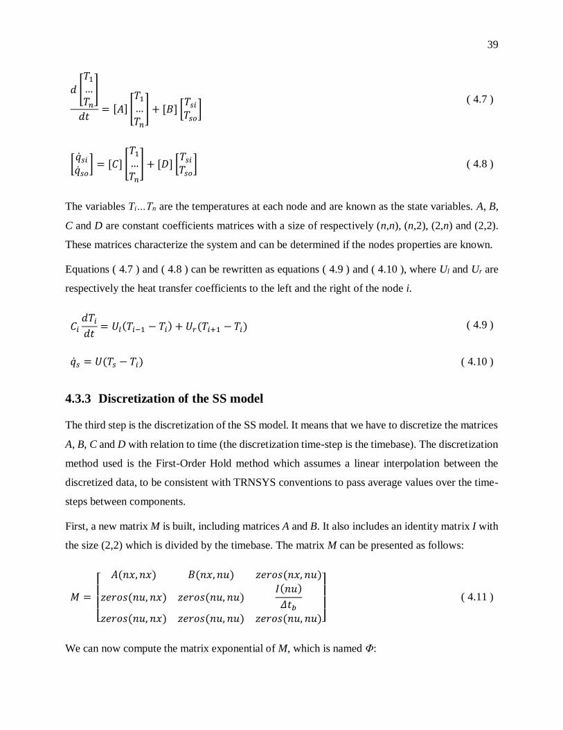
39
𝑑 [𝑇1…𝑇𝑛
]
𝑑𝑡= [𝐴] [
𝑇1…𝑇𝑛
] + [𝐵] [𝑇𝑠𝑖𝑇𝑠𝑜]
( 4.7 )
[��𝑠𝑖��𝑠𝑜] = [𝐶] [
𝑇1…𝑇𝑛
] + [𝐷] [𝑇𝑠𝑖𝑇𝑠𝑜] ( 4.8 )
The variables Ti…Tn are the temperatures at each node and are known as the state variables. A, B,
C and D are constant coefficients matrices with a size of respectively (n,n), (n,2), (2,n) and (2,2).
These matrices characterize the system and can be determined if the nodes properties are known.
Equations ( 4.7 ) and ( 4.8 ) can be rewritten as equations ( 4.9 ) and ( 4.10 ), where Ul and Ur are
respectively the heat transfer coefficients to the left and the right of the node i.
𝐶𝑖𝑑𝑇𝑖𝑑𝑡
= 𝑈𝑙(𝑇𝑖−1 − 𝑇𝑖) + 𝑈𝑟(𝑇𝑖+1 − 𝑇𝑖) ( 4.9 )
��𝑠 = 𝑈(𝑇𝑠 − 𝑇𝑖) ( 4.10 )
4.3.3 Discretization of the SS model
The third step is the discretization of the SS model. It means that we have to discretize the matrices
A, B, C and D with relation to time (the discretization time-step is the timebase). The discretization
method used is the First-Order Hold method which assumes a linear interpolation between the
discretized data, to be consistent with TRNSYS conventions to pass average values over the time-
steps between components.
First, a new matrix M is built, including matrices A and B. It also includes an identity matrix I with
the size (2,2) which is divided by the timebase. The matrix M can be presented as follows:
𝑀 =
[ 𝐴(𝑛𝑥, 𝑛𝑥) 𝐵(𝑛𝑥, 𝑛𝑢) 𝑧𝑒𝑟𝑜𝑠(𝑛𝑥, 𝑛𝑢)
𝑧𝑒𝑟𝑜𝑠(𝑛𝑢, 𝑛𝑥) 𝑧𝑒𝑟𝑜𝑠(𝑛𝑢, 𝑛𝑢)𝐼(𝑛𝑢)
𝛥𝑡𝑏𝑧𝑒𝑟𝑜𝑠(𝑛𝑢, 𝑛𝑥) 𝑧𝑒𝑟𝑜𝑠(𝑛𝑢, 𝑛𝑢) 𝑧𝑒𝑟𝑜𝑠(𝑛𝑢, 𝑛𝑢)]
( 4.11 )
We can now compute the matrix exponential of M, which is named Φ:
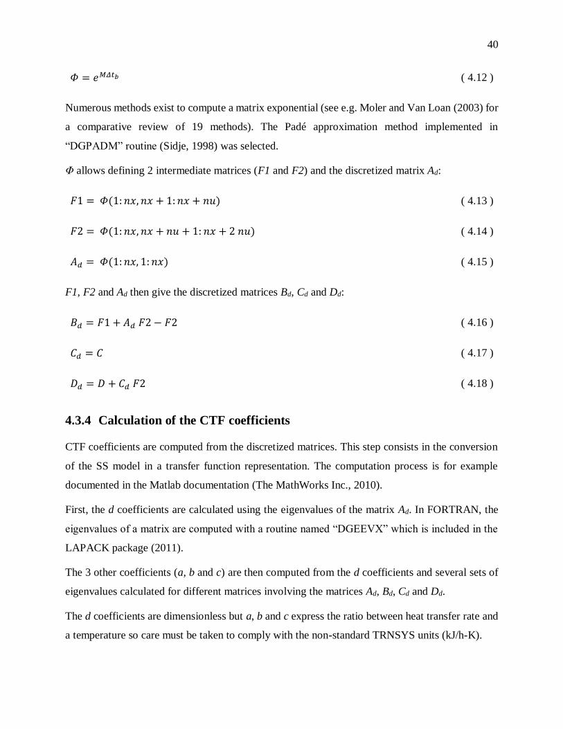
40
𝛷 = 𝑒𝑀𝛥𝑡𝑏 ( 4.12 )
Numerous methods exist to compute a matrix exponential (see e.g. Moler and Van Loan (2003) for
a comparative review of 19 methods). The Padé approximation method implemented in
“DGPADM” routine (Sidje, 1998) was selected.
Φ allows defining 2 intermediate matrices (F1 and F2) and the discretized matrix Ad:
𝐹1 = 𝛷(1: 𝑛𝑥, 𝑛𝑥 + 1: 𝑛𝑥 + 𝑛𝑢) ( 4.13 )
𝐹2 = 𝛷(1: 𝑛𝑥, 𝑛𝑥 + 𝑛𝑢 + 1: 𝑛𝑥 + 2 𝑛𝑢) ( 4.14 )
𝐴𝑑 = 𝛷(1: 𝑛𝑥, 1: 𝑛𝑥) ( 4.15 )
F1, F2 and Ad then give the discretized matrices Bd, Cd and Dd:
𝐵𝑑 = 𝐹1 + 𝐴𝑑 𝐹2 − 𝐹2 ( 4.16 )
𝐶𝑑 = 𝐶 ( 4.17 )
𝐷𝑑 = 𝐷 + 𝐶𝑑 𝐹2 ( 4.18 )
4.3.4 Calculation of the CTF coefficients
CTF coefficients are computed from the discretized matrices. This step consists in the conversion
of the SS model in a transfer function representation. The computation process is for example
documented in the Matlab documentation (The MathWorks Inc., 2010).
First, the d coefficients are calculated using the eigenvalues of the matrix Ad. In FORTRAN, the
eigenvalues of a matrix are computed with a routine named “DGEEVX” which is included in the
LAPACK package (2011).
The 3 other coefficients (a, b and c) are then computed from the d coefficients and several sets of
eigenvalues calculated for different matrices involving the matrices Ad, Bd, Cd and Dd.
The d coefficients are dimensionless but a, b and c express the ratio between heat transfer rate and
a temperature so care must be taken to comply with the non-standard TRNSYS units (kJ/h-K).

41
4.3.5 Check of the generated CTF coefficients
The validity of the computed CTF coefficients is checked using Equation ( 4.3 ): the calculated U-
values must be within 0.001% of the “actual” value (i.e. computed from the layers description).
4.4 Example
This section illustrates the CTF coefficients generation by a simple example of a slab with 3 nodes.
The example (Figure 4-1) is a concrete slab with a thickness L of 0.3 m, a density ρ of 2200 kg/m³,
a specific heat Cp of 0.84 kJ/kg-K and a thermal conductivity k of 1.7 W/m-K. The inside and
outside film coefficients hi and ho have a value of respectively 8.3 and 34.5 W/m²-K (in TRNSYS,
these coefficients would be handled in a different part of the program and would not be included
in the CTF coefficients).
Figure 4-1: Scheme of a three-node example
Once the nodes are defined, the A, B, C and D matrices of the SS model can be calculated. The
thermal capacity and resistance (or U-value) for each node are presented in equations ( 4.19 ) to
( 4.24 ):
𝐶𝑤 = 𝜌 𝐶𝑝 𝐿 = 2200 × 840 × 0.3 = 554400𝐽
𝑚²𝐾 ( 4.19 )
𝐶1 = 𝐶3 =554400
4= 138600
𝐽
𝑚2𝐾 ( 4.20 )
𝐶2 =554400
2= 277200
𝐽
𝑚2𝐾 ( 4.21 )
𝑈1 =1
𝑅1= ℎ𝑖 = 8.3
𝑊
𝑚2𝐾 ( 4.22 )

42
𝑈2 = 𝑈3 =1
𝑅2=𝑘
𝐿2
=1.7
0.15= 11.33
𝑊
𝑚2𝐾 ( 4.23 )
𝑈4 =1
𝑅4= ℎ𝑜 = 34.5
𝑊
𝑚2𝐾 ( 4.24 )
Differential equations similar to equation ( 4.9 ) can then be written for each node:
𝑑𝑇1𝑑𝑡
=𝑈1
𝐶1(𝑇𝑖 − 𝑇1) +
𝑈2
𝐶1(𝑇2 − 𝑇1) =
8.3
138600(𝑇𝑖 − 𝑇1) +
11.33
138600(𝑇2 − 𝑇1) ( 4.25 )
𝑑𝑇2𝑑𝑡
=𝑈2
𝐶2(𝑇1 − 𝑇2) +
𝑈3
𝐶2(𝑇3 − 𝑇2) =
11.33
277200(𝑇1 − 𝑇2) +
11.33
277200(𝑇3 − 𝑇2) ( 4.26 )
𝑑𝑇3𝑑𝑡
=𝑈3
𝐶3(𝑇2 − 𝑇3) +
𝑈4
𝐶3(𝑇𝑜 − 𝑇3) =
11.33
138600(𝑇2 − 𝑇3) +
34.5
138600(𝑇𝑜 − 𝑇3) ( 4.27 )
Equations ( 4.25 ) to ( 4.27 ) can be written in a matrix form, where the 3-by-3 matrix is A and the
3-by-2 matrix is B in the SS model:
𝑑
𝑑𝑡[𝑇1𝑇2𝑇3
] =
[ −
19.63
138600
11.33
1386000
11.33
277200−22.66
277200
11.33
277200
011.33
138600−45.83
138600]
[𝑇1𝑇2𝑇3
]
+
[ 8.3
1386000
0 0
034.5
138600]
[𝑇𝑖𝑇𝑜]
( 4.28 )
Heat flows are computed from the first and last nodes and boundary conditions:
��𝑠𝑖 = ℎ𝑖(𝑇𝑖 − 𝑇1) = 8.3 (𝑇𝑖 − 𝑇1) ( 4.29 )
��𝑠𝑜 = ℎ𝑜(𝑇𝑜 − 𝑇3) = 34.5 (𝑇𝑜 − 𝑇3) ( 4.30 )
Or, in a matrix form:

43
[��𝑠𝑖��𝑠𝑜] = [
−8.3 0 00 0 −34.5
] [𝑇1𝑇2𝑇3
] + [8.3 00 34.5
] [𝑇𝑖𝑇𝑜] ( 4.31 )
The 2-by-3 and 2-by-2 matrices in equation ( 4.31 ) are respectively C and D in the SS model.
The four matrices are discretized for a time-step of 1 hour (3600 seconds):
𝐴𝑑 = [0.6147 0.1999 0.011420.09994 0.7725 0.073530.01142 0.1471 0.3133
] ( 4.32 )
𝐵𝑑 = [0.1355 0.010290.02049 0.061370.002475 0.3142
] ( 4.33 )
𝐶𝑑 = [−8.3 0 00 0 −34.5
] ( 4.34 )
𝐷𝑑 = [7.537 −0.009171
−0.009171 23.68] ( 4.35 )
The CTF coefficients are calculated from the discretized matrices as explained previously. Table
4-1 shows the results:
Table 4-1: Values of the CTF coefficients
a b c d
1 85.2408 0.033 27.1343 1.0000
2 -183.9657 0.2512 -50.1883 -1.7004
3 127.8714 0.169 28.1085 0.8785
4 -28.6833 0.01 -4.5913 -0.1361
Sum 0.4632 0.4632 0.4632 0.042
U-value [kJ/h-m²-K] 11.0286 11.0286 11.0286 /
The actual U-value (including the film coefficients) of the concrete slab is 11.045 kJ/h-m²-K while
the U-value calculated with the coefficients is 11.029 kJ/h-m²-K. The observed error is 0.15 %
which is greater than the limit of 0.001 %. So the coefficients should be considered as non-reliable.
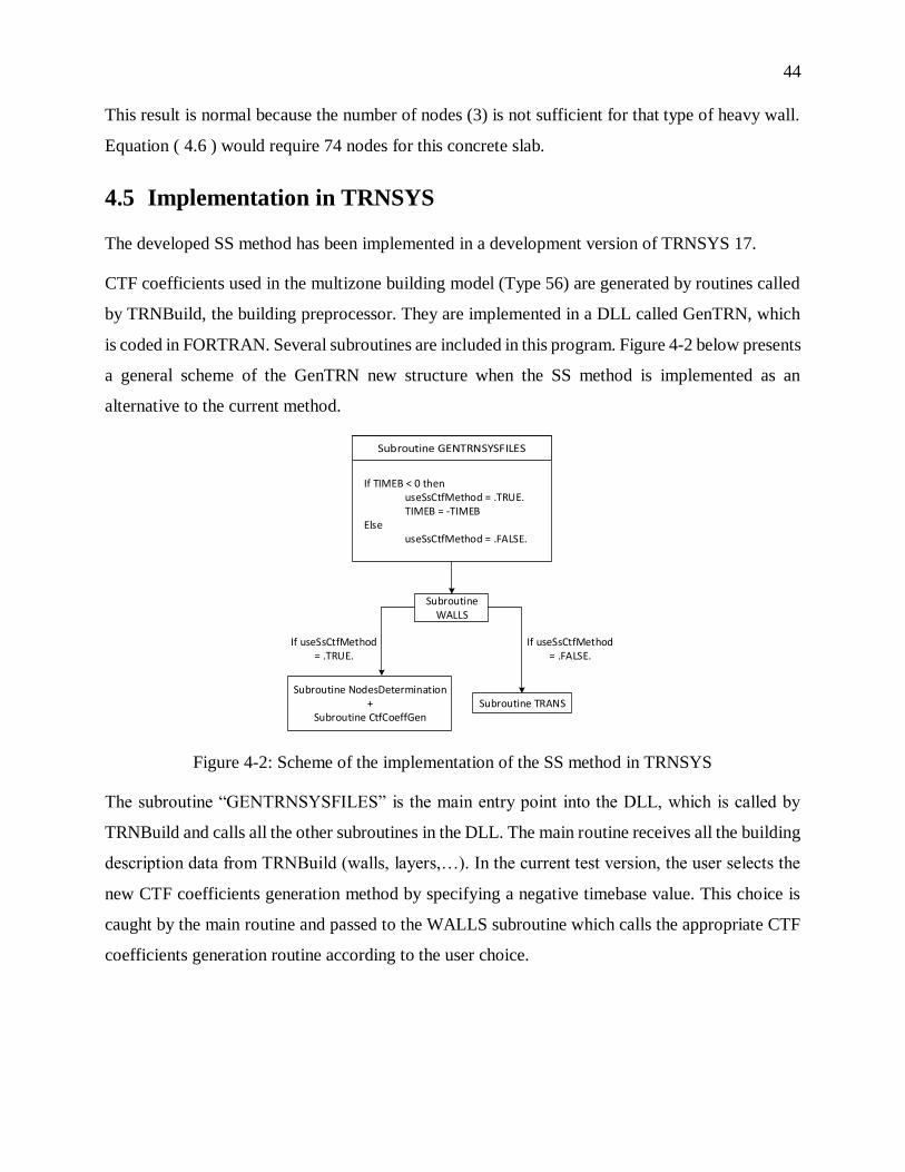
44
This result is normal because the number of nodes (3) is not sufficient for that type of heavy wall.
Equation ( 4.6 ) would require 74 nodes for this concrete slab.
4.5 Implementation in TRNSYS
The developed SS method has been implemented in a development version of TRNSYS 17.
CTF coefficients used in the multizone building model (Type 56) are generated by routines called
by TRNBuild, the building preprocessor. They are implemented in a DLL called GenTRN, which
is coded in FORTRAN. Several subroutines are included in this program. Figure 4-2 below presents
a general scheme of the GenTRN new structure when the SS method is implemented as an
alternative to the current method.
Figure 4-2: Scheme of the implementation of the SS method in TRNSYS
The subroutine “GENTRNSYSFILES” is the main entry point into the DLL, which is called by
TRNBuild and calls all the other subroutines in the DLL. The main routine receives all the building
description data from TRNBuild (walls, layers,…). In the current test version, the user selects the
new CTF coefficients generation method by specifying a negative timebase value. This choice is
caught by the main routine and passed to the WALLS subroutine which calls the appropriate CTF
coefficients generation routine according to the user choice.
Subroutine WALLS
If TIMEB < 0 thenuseSsCtfMethod = .TRUE.TIMEB = -TIMEB
ElseuseSsCtfMethod = .FALSE.
Subroutine NodesDetermination+
Subroutine CtfCoeffGenSubroutine TRANS
If useSsCtfMethod = .FALSE.
If useSsCtfMethod = .TRUE.

45
4.6 Wall tests in TRNSYS
Extensive tests were performed to debug and quality-check the new CTF coefficients generation
method. This paper reports on 2 wall types: an insulated concrete form (ICF) wall and a plain
wooden wall. The characteristics of each slab are presented in the following table (from inside to
outside).
Table 4-2: Description of the presented walls
Slabs L [m] k [W/(m-K)] ρ [kg/m³] Cp [kJ/(kg-K)] R [m²-K/W]
ICF Wall-only U-value: 0.188 W/(m²-K)
G01 - Gypsum board 0.016 0.16 800 1.09 0.100
I03 - EPS (expanded
polystyrene) board 0.076 0.03 43 1.21 2.533
M15 - Heavyweight
concrete 0.203 1.95 2240 0.9 0.104
I03 - EPS board 0.076 0.03 43 1.21 2.533
F07 - Stucco 0.025 0.72 1856 0.84 0.035
Wood wall Wall-only U-value: 0.260 W/(m²-K)
Wood 0.500 0.130 600 1.88 3.846
The plain 50-cm wooden wall is an extreme case that illustrated the limits of the CTF method (as
currently implemented and with the new coefficients generation method).
The scenario that we have tested is the one presented in the Figure 4-3. It represents a typical set-
back scenario.
The outside temperature is kept constant at 0°C. No radiative heat flows are considered. The
heating system power is initially set to maintain a steady-state indoor temperature of 20°C. The
heating system is then stopped for 4 hours, and restarted with a heating power equal to 1.5 times
the initial value.
The simulation time-step is one minute and the inside and outside convection coefficients have a
value of 8.3 and 34.5 W/m²-K, respectively.

46
Figure 4-3: Description of the presented scenario
In the following four graphs, three kind of results are presented: firstly, in dotted lines, the results
coming from the current version of TRNSYS; secondly, in dashed lines, the results performed by
using the SS method for generating the CTF coefficients; thirdly, in solid lines, a reference solution
implemented in Matlab (The MathWorks Inc., 2010) by simulating a discretized wall model with
a large number of nodes. All graphs present the evolution of the inside surface temperature
according to time.
The first two graphs (Figure 4-4 and Figure 4-5) concern the ICF wall (Figure 4-5 is a zoom into
Figure 4-4 to highlight the differences between the curves). The results show that the original and
modified versions of TRNSYS match the reference solution at the end of each timebase but the
presence of a stair-step effect is influenced by that timebase. The minimum timebase value that can
be reached with the new method is 12 minutes, while it was 1 hour with the DRF method.
The next two graphs are about the plain wooden wall with a thickness of 0.5 m, the second one
being a zoom where the minimum temperature is reached. This wall is not typical from walls
encountered in real buildings but it allows highlighting problems with the CTF method. These
problems appear clearly in the graphs. The results generated by the current and modified versions
of TRNSYS are affected by a stair-step effect. That effect is more pronounced for the current
TRNSYS version (minimum timebase value = 3 hours, vs. 1 hour for the new method). During the
temperature drop, the modified version behaves better while it is the opposite during the
temperature increase. It is not clear at this stage why the new CTF coefficient generation shows an
offset in addition to the stair-step effect. This will be investigated in the future.
Figure 4-7 shows that both curves present a negative peak that is not present in the reference
solution. Again, future work will aim at clarifying why the response of the wooden wall is incorrect.

47
Figure 4-4: Evolution of the inside surface temperature for an ICF wall
Figure 4-5: Evolution of the inside surface temperature for an ICF wall (zoom)
4000 4005 4010 4015 4020 4025 403016
17
18
19
20
21
22
23
Time [h]
Tem
pera
ture
[°C
]
Original - 1 h
Modified - 12 min
Reference
4018 4018.5 4019 4019.5 4020 4020.5 402117
17.2
17.4
17.6
17.8
18
18.2
18.4
18.6
18.8
19
Time [h]
Tem
pera
ture
[°C
]
Original - 1 h
Modified - 12 min
Reference
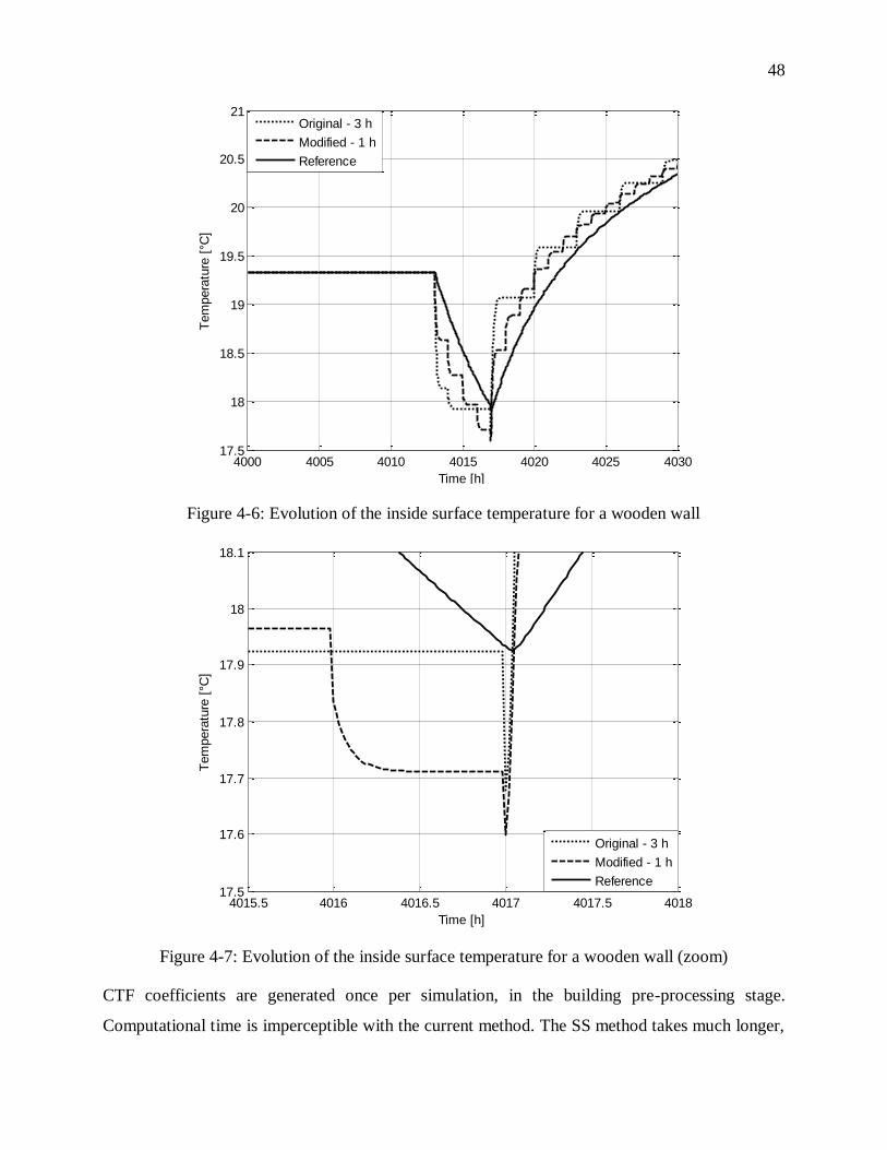
48
Figure 4-6: Evolution of the inside surface temperature for a wooden wall
Figure 4-7: Evolution of the inside surface temperature for a wooden wall (zoom)
CTF coefficients are generated once per simulation, in the building pre-processing stage.
Computational time is imperceptible with the current method. The SS method takes much longer,
4000 4005 4010 4015 4020 4025 403017.5
18
18.5
19
19.5
20
20.5
21
Time [h]
Tem
pera
ture
[°C
]
Original - 3 h
Modified - 1 h
Reference
4015.5 4016 4016.5 4017 4017.5 401817.5
17.6
17.7
17.8
17.9
18
18.1
Time [h]
Tem
pera
ture
[°C
]
Original - 3 h
Modified - 1 h
Reference
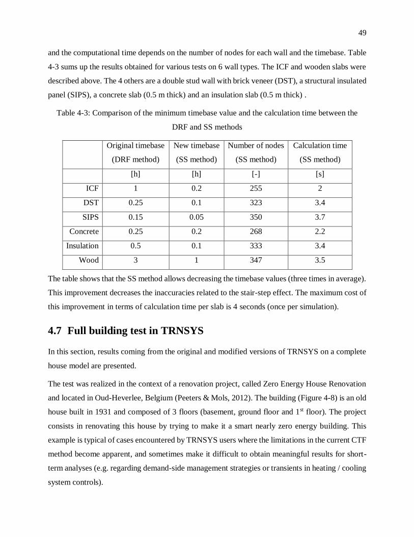
49
and the computational time depends on the number of nodes for each wall and the timebase. Table
4-3 sums up the results obtained for various tests on 6 wall types. The ICF and wooden slabs were
described above. The 4 others are a double stud wall with brick veneer (DST), a structural insulated
panel (SIPS), a concrete slab (0.5 m thick) and an insulation slab (0.5 m thick) .
Table 4-3: Comparison of the minimum timebase value and the calculation time between the
DRF and SS methods
Original timebase
(DRF method)
New timebase
(SS method)
Number of nodes
(SS method)
Calculation time
(SS method)
[h] [h] [-] [s]
ICF 1 0.2 255 2
DST 0.25 0.1 323 3.4
SIPS 0.15 0.05 350 3.7
Concrete 0.25 0.2 268 2.2
Insulation 0.5 0.1 333 3.4
Wood 3 1 347 3.5
The table shows that the SS method allows decreasing the timebase values (three times in average).
This improvement decreases the inaccuracies related to the stair-step effect. The maximum cost of
this improvement in terms of calculation time per slab is 4 seconds (once per simulation).
4.7 Full building test in TRNSYS
In this section, results coming from the original and modified versions of TRNSYS on a complete
house model are presented.
The test was realized in the context of a renovation project, called Zero Energy House Renovation
and located in Oud-Heverlee, Belgium (Peeters & Mols, 2012). The building (Figure 4-8) is an old
house built in 1931 and composed of 3 floors (basement, ground floor and 1st floor). The project
consists in renovating this house by trying to make it a smart nearly zero energy building. This
example is typical of cases encountered by TRNSYS users where the limitations in the current CTF
method become apparent, and sometimes make it difficult to obtain meaningful results for short-
term analyses (e.g. regarding demand-side management strategies or transients in heating / cooling
system controls).

50
Figure 4-8: Picture of the house in project ZEHR (Zero Energy House Renovation) (Peeters &
Mols, 2012)
The presented results focus on the evolution of the operative temperature in the kitchen, as shown
in Figure 4-9.
Figure 4-9: Plan of the house’s ground floor (Peeters & Mols, 2012)
Table 4 below describes the external wall of the kitchen, which is a highly insulated (U = 0.115
W/m²-K) and heavy slab.
Table 4-4: Description of the external wall in the kitchen (Peeters & Mols, 2012)
L [m] k [W/m-K] ρ [kg/m³] Cp [kJ/kg-K] R [m²-K/W]
Cavity / / / / 0.140
Foamglass 0.300 0.038 130 0.840 7.895
Brick 0.330 0.500 1500 0.840 0.660
Plaster 0.010 0.700 1400 0.840 0.014
The setback scenario presented above is extended to this case. The outside temperature is fixed at
0°C. There are no solar gains. The only room to be heated is the kitchen (convective heater). The
heating system stops during 4 hours before a restart with more power (1.5 times the initial power).

51
The simulation has been carried out twice: firstly, with the original version of TRNSYS (DRF
method – Timebase = 5 hours, the minimum achievable) and secondly, with the modified version
of TRNSYS (SS method – Timebase = 1.5 hours, the minimum achievable).
Figure 4-10 below shows the evolution of the operative temperature in the kitchen according to
time. The results present a clear difference between the 2 methods (DRF and SS) for generating
the CTF coefficients. The SS method allows reducing the stair-step effect, as shown in the single-
wall examples. The observed maximum and mean temperature differences between the 2 methods
are respectively 0.49 and 0.16 °C.
Another important parameter to take into account is the impact of the method on the computational
time during the simulation (and not during the CTF coefficients generation). For a 168-day
simulation with a time-step of 1 minute, the computational times for the original and modified
versions of TRNSYS are respectively 21 and 23 minutes.
Figure 4-10: Evolution of the operative temperature in the kitchen [corrected after publication]
4.8 Discussion and conclusions
This paper describes the implementation of a new CTF coefficients generation method in TRNSYS.
The method was successfully implemented in a development version of the TRNSYS building pre-
processor (TRNBuild). This work is intended to respond to problems faced by TRNSYS users who

52
simulate heavy, highly insulated walls and want to perform short term analyses to study demand-
side management strategies or transients in heating and cooling system controls.
The proposed method alleviates the stair-step effect that occurs in these circumstances, allowing to
reduce the minimum timebase by a factor of 3 in average. It provides very satisfactory results in
some cases for time-steps down to the order of one minute. Some walls present more difficulties
such as the extreme 50-cm thick plain wooden slab selected for our test. In these cases, the new
method delivers some improvements regarding the stair-step effects but does not compare
favorably with a reference solution. Further work will aim at better understanding the limitations
of the CTF method while the new method is released to more TRNSYS users.
The impact on computational time to generate the CTF coefficients is significant, but this operation
only takes place once per simulation and the cost amounts to a few seconds per wall type. The
impact on simulation time in a realistic case is acceptable (10% increase).
Nomenclature
A, B, C and D State-space matrices
a, b, c and d CTF coefficients
C Thermal capacity [J/m²-K]
Cp Specific heat [J/kg-K]
Fo Fourier number
h Convection coefficient [W/m²-K]
k Thermal conductivity [W/m-K]
L Thickness [m]
n Number of coefficients or nodes
nx Nodes number
nu Inputs number (= 2)
�� Heat flow [W or kJ/h]
R Thermal resistance [m²-K/W]

53
T Temperature [°C or K]
t Time [s]
U Heat transfer coefficient [W/m²-K]
x Position [m]
𝛥𝑡𝑏 Timebase [s]
Greek symbols
α Thermal diffusivity [m²/s]
Δ Difference
ρ Density [kg/m³]
Subscript
d Discretized
i Inside or i-node
k Number of CTF coefficient
l Left
o Outside
r Right
s Surface
w Wall
Acknowledgements
The research work presented in this paper is financially supported by a grant of Hydro-Québec,
FRQNT (Fonds de Recherche du Québec de Recherche en Nature et Technologies) and NSERC
(Natural Sciences and Engineering Research Council of Canada). Moreover the presentation of the
full building test in this paper has been possible thanks to the cooperation of Leen Peeters who
works on the “Zero Energy House Renovation” project.

54
References
Delcroix, B., Kummert, M., Daoud, A., & Hiller, M. (2012). Conduction transfer functions in
TRNSYS multizone building model: current implementation, limitations and possible
improvements. SimBuild (p. 8). Madison, Wisconsin.
Energy Systems Research Unit. (1998). ESP-r User Guide: The ESP-r System for Building
Energy Simulation. Glasgow.
EnergyPlus Documentation. (2012). Engineering Reference (p. 1247).
LAPACK. (2011). DGEEVX: computation of the eigenvalues of a general matrix. Retrieved
from http://www.netlib.org/lapack/individualroutines.html
Li, X. Q., Chen, Y., Spitler, J. D., & Fisher, D. (2009). Applicability of calculation methods for
conduction transfer function of building constructions. International Journal of Thermal
Sciences, 48(7), 1441–1451. doi:10.1016/j.ijthermalsci.2008.11.006
Mitalas, G. P., & Arseneault, J. G. (1972). Fortran IV program to calculate z-transfer functions
for the calculation of transient heat transfer through walls and roofs. Division of Building
research, National Research Council Canada. Retrieved from http://nparc.cisti-icist.nrc-
cnrc.gc.ca/npsi/ctrl?action=shwart&index=an&req=5752842
Moler, C., & Van Loan, C. (2003). Nineteen Dubious Ways to Compute the Exponential of a
Matrix, Twenty-Five Years Later. SIAM Review, 45(1), 3–49.
Myers, G. E. (1971). Analytical methods in conduction heat transfer (McGraw-Hil.). New-York.
Peeters, L., & Mols, R. (2012). Zero Energy House Renovation. Retrieved February 8, 2013,
from http://www.zehr.be
Seem, J. E. (1987). Modeling of heat transfer in buildings. University of Wisconsin, Madison.

55
Sidje, R. B. (1998). Expokit: a software package for computing matrix exponentials. ACM
Transactions on Mathematical Software, 24(1), 130–156.
Stephenson, D. G., & Mitalas, G. P. (1971). Calculation of heat conduction transfer functions for
multi-layer slabs. ASHRAE Transactions, 77(2), 117–126. Retrieved from http://nparc.cisti-
icist.nrc-cnrc.gc.ca/npsi/ctrl?action=shwart&index=an&req=5757086&lang=en
The MathWorks Inc. (2010). Matlab help. Natick, MA, USA.
TRANSSOLAR Energietechnik Gmbh. (2011). TRNSYS 17 - Multizone building modeling with
Type 56 and TRNBuild (p. 258). Stuttgart.

56
CHAPTER 5 ADDITIONAL COMMENTS ON ARTICLE 1
This chapter presents additional details about the conditions in which the CTF method yields
accurate results. These conditions are compared to the stability conditions for finite-difference
methods, to illustrate the complementarity between the two approaches.
In TRNSYS, the validity of the CTF method is assessed by a simple condition: the sum of each
coefficients set (a, b and c) must be higher than or equal to 0.0005 such as:
∑ 𝑎𝑡−𝑘𝛥𝑡𝑏𝑛𝑎 𝑘=0 ≥ 0.0005 ; ∑ 𝑏𝑡−𝑘𝛥𝑡𝑏
𝑛𝑏 𝑘=0 ≥ 0.0005 ; ∑ 𝑐𝑡−𝑘𝛥𝑡𝑏
𝑛𝑐 𝑘=0 ≥ 0.0005 ( 5.1 )
If this condition is not met, the CTF coefficients are not generated and an error window (see Figure
5-1) prompts the user to adapt the timebase value. As shown in Chapter 4, these three sums must
have the same value.
Figure 5-1: Error window when TRNBuild fails to generate transfer function coefficients
The sum of each coefficients set is directly proportional to the Fourier number. For example, Table
5-1 presents the evolution of the sum of a set of CTF coefficients and the Fourier number as a
function of the timebase for a wall case presented in section 4.6, i.e. the plain wooden wall.
Table 5-1: Evolution of the sum of a set of CTF coefficients and the Fourier number as a function
of the timebase for the plain wooden wall
Timebase [h] Sum of a set of CTF coefficients Fourier number
3 0.0008 0.0050
4 0.0028 0.0066
5 0.0064 0.0083
This condition avoids therefore generating CTF coefficients as soon as the wall becomes too
insulated and / or thermally heavy, i.e. a wall with a low Fourier number. Maestre et al. (2014)
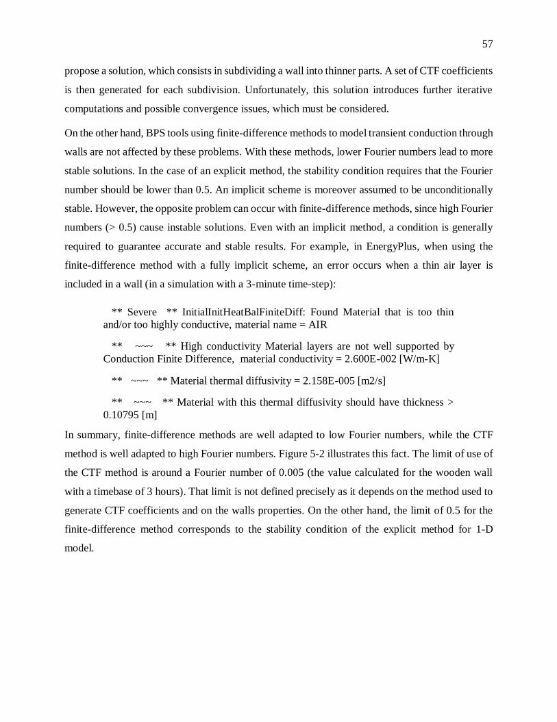
57
propose a solution, which consists in subdividing a wall into thinner parts. A set of CTF coefficients
is then generated for each subdivision. Unfortunately, this solution introduces further iterative
computations and possible convergence issues, which must be considered.
On the other hand, BPS tools using finite-difference methods to model transient conduction through
walls are not affected by these problems. With these methods, lower Fourier numbers lead to more
stable solutions. In the case of an explicit method, the stability condition requires that the Fourier
number should be lower than 0.5. An implicit scheme is moreover assumed to be unconditionally
stable. However, the opposite problem can occur with finite-difference methods, since high Fourier
numbers (> 0.5) cause instable solutions. Even with an implicit method, a condition is generally
required to guarantee accurate and stable results. For example, in EnergyPlus, when using the
finite-difference method with a fully implicit scheme, an error occurs when a thin air layer is
included in a wall (in a simulation with a 3-minute time-step):
** Severe ** InitialInitHeatBalFiniteDiff: Found Material that is too thin
and/or too highly conductive, material name = AIR
** ~~~ ** High conductivity Material layers are not well supported by
Conduction Finite Difference, material conductivity = 2.600E-002 [W/m-K]
** ~~~ ** Material thermal diffusivity = 2.158E-005 [m2/s]
** ~~~ ** Material with this thermal diffusivity should have thickness >
0.10795 [m]
In summary, finite-difference methods are well adapted to low Fourier numbers, while the CTF
method is well adapted to high Fourier numbers. Figure 5-2 illustrates this fact. The limit of use of
the CTF method is around a Fourier number of 0.005 (the value calculated for the wooden wall
with a timebase of 3 hours). That limit is not defined precisely as it depends on the method used to
generate CTF coefficients and on the walls properties. On the other hand, the limit of 0.5 for the
finite-difference method corresponds to the stability condition of the explicit method for 1-D
model.

58
Figure 5-2: Complementarity of the CTF method and the finite-difference methods
Figure 5-2 also highlights the complementarity of both methods. This complementarity can be
exploited in TRNSYS, where an external type modeling a wall with a finite-difference method can
be linked to two boundary walls modeled with the CTF method in Type 56 (“Multizone building
model”).
This method has been applied on the example presented in section 4.7 to show the merits of using
an external type to model a highly resistive and heavy wall. Peeters and Mols (2012) presented a
renovation project called “Zero Energy House Renovation” and located in Oud-Heverlee in
Belgium. The building is an old house composed of 3 floors, including a basement. The renovation
works required to add insulation to the existing building. In particular, the roof poses a challenge
to the CTF method, and requires using a timebase greater than or equal to 5 hours for the simulation,
because of its very low thermal diffusivity. Table 5-2 presents the composition of this wall from
outside to inside.
Table 5-2: Composition of the roof of the studied case (from outside to inside)
Material Thickness
[m]
Thermal conductivity
[W/m-K]
Density
[kg/m³]
Specific heat
[kJ/kg-K]
Cellulosic insulation 0.380 0.040 350 2.150
Wood fiber panel (Celit 4D) 0.020 0.055 270 2.068
Plaster 0.010 0.700 1400 0.840
The test case to evaluate the efficiency of the proposed method is illustrated in Figure 5-3. The
inside temperature is kept constant at 20 °C and the outside temperature changes by steps.

59
Figure 5-3: Test case with temperature step-changes
Two simulation configurations are tested. For all simulations, a time-step of 6 minutes is used.
First, the entire wall is modeled in Type 56 using the CTF method with a timebase of 5 hours
(which is the minimum achievable). Secondly, a small part of the wall (1 cm of cellulosic insulation
and the 1-cm plaster layer) is modeled using the CTF method while the other part (37 cm of
cellulosic insulation and the wood fiber panel) is modeled in an external type using a finite-
difference method. The last configuration allows using a timebase of 6 minutes, i.e. equivalent to
the simulation time-step.
Results are presented for the outside surface temperature in Figure 5-4. Discrepancies appears with
the CTF method where the gap between the timebase (5 hours) and the time-step (6 minutes) causes
a strong stair-step effect. Figure 5-4 (b) focuses on the corrections performed by the CTF method
at the 30th, 35th and 40th hours, i.e. every 5 hours. On the other hand, using an external type for
modeling the wall with a finite-difference method allows producing correct results without stair-
step effects.
Figure 5-4: Results comparison between both configurations

60
CHAPTER 6 ARTICLE 2: INFLUENCE OF EXPERIMENTAL
CONDITIONS ON MEASURED THERMAL PROPERTIES USED TO
MODEL PHASE CHANGE MATERIALS
Delcroix, B., Kummert, M., Daoud, A., Bouchard, J., (2015). Influence of experimental conditions
on measured thermal properties used to model phase change materials. Building Simulation: An
International Journal. doi:10.1007/s12273-015-0241-8
Abstract
Modeling phase change materials (PCMs) thermal behavior requires solving a system of non-linear
equations to account for temperature-dependent thermal capacity and thermal conductivity. These
properties depend on the PCM temperature and state (solid, liquid or mushy). Most models rely on
enthalpy-temperature or specific heat-temperature curves to consider the variable thermal capacity
during heating and cooling processes. These curves are generally obtained through experimental
methods such as a Differential Scanning Calorimetry (DSC) test or the T-history method.
Significant differences can be observed between the results of these methods, due to different
experimental conditions. In order to clarify the influence of experimental conditions,
experimentations on a bio-based PCM are performed with varying heat transfer rates and different
configurations (PCM samples and PCM-equipped walls). Enthalpy-temperature or specific heat-
temperature curves are computed for each case using an inverse method. A comparison between
the results obtained with different methods and different heat transfer rates shows significant
differences. The phase change temperature range obtained with the inverse method applied to the
PCM samples is larger than the range obtained with the DSC test. The tests on the PCM-equipped
walls show that varying heat transfer rates have a significant impact on the phase change
temperature range and the hysteresis between heating and cooling curves. Higher rates increase the
hysteresis and shift the phase change temperature range towards colder temperatures. Given the
observed differences between properties obtained from different experimental conditions, it is
recommended to carefully select the method used to define PCM enthalpy-temperature curves,
taking into account the modeling application (PCM configuration and expected heating / cooling
rates).

61
Keywords: Phase change material (PCM); Latent heat storage capacity; Enthalpy-temperature
curve; Differential Scanning Calorimetry (DSC); Inverse modeling method
Nomenclature
𝐴 Heat-exchange surface [m²]
Bi Biot number [-]
𝐶 Capacitance [J/m²-K]
𝐶𝑝 Specific heat [J/g-K]
ℎ Enthalpy [J/g]
ℎ𝑔 Global heat transfer coefficient [W/m²-K]
𝑘 Thermal conductivity [W/m-K]
𝐿𝑐 Characteristic length [m]
𝑚 Mass [g]
𝑅 Thermal resistance [m².K/W]
𝑟 Radius [m]
S Surface
𝑇 Temperature [°C]
𝑡 Time [s]
𝑈 Heat transfer coefficient [W/m²-K]
∆ℎ Enthalpy variation [J/g]
∆𝑥 Node interval [m]
𝜌 Density [kg/m³]
Subscripts
𝑐 Cooling
𝑒𝑥𝑝 Experimental

62
𝑓 Final
ℎ Heating
𝑖 Initial
𝑖𝑛 Center or inside
𝑙 Left or liquid
𝑛 Node
𝑜𝑢𝑡 Outside
𝑝𝑐𝑚 Phase change material
𝑟 Right
𝑠 Sample or solid
𝑠𝑖 Inside surface
𝑠𝑖𝑚 Simulated
𝑠𝑜 Outside surface
𝑤 Water
6.1 Introduction
Latent heat storage systems using Phase Change Materials (PCMs) are increasingly used and
studied for building applications. PCMs offer a high energy storage capacity and a nearly
isothermal phase change, which help reducing peaks in space heating and cooling loads and
maintaining thermal comfort. Several authors have documented PCM properties and possible
applications. Reviews presented by Zalba et al. (2003), Sharma et al. (2009) and Baetens et al.
(2010) document PCM classifications and a wide range of PCMs with their most important
properties. Zalba et al. (2003) provide a large overview of possible applications, while Sharma et
al. (2009) and Baetens et al. (2010) focus on solar and building applications. Mehling and Cabeza
(2008) also offer an in-depth description of the theoretical aspects and multiple applications related
to PCM.

63
The effective heat capacity (Goodrich, 1978; Yao & Chait, 1993) and enthalpy (Voller & Cross,
1981) methods are often used to model the PCM non-linear thermal behavior in buildings. Building
energy performance simulation programs such as ESP-r (Energy Systems Research Unit, 1998),
EnergyPlus (Crawley et al., 2001) and TRNSYS (Klein et al., 2012) use these methods. The
effective thermal capacity method is integrated into the ESP-r building model (Heim & Clarke,
2004), while the enthalpy method is implemented into EnergyPlus (Pedersen, 2007; Shrestha et al.,
2011; Tabares-Velasco, Christensen, & Bianchi, 2012). Several component models (known as
“Types”) using both methods have been implemented in TRNSYS (Castell et al., 2009; A Dentel
& Stephan, 2010; Ibánez et al., 2005; Kuznik et al., 2010; Poulad et al., 2011; Schranzhofer et al.,
2006). Few models are able to represent specific PCM effects such as hysteresis and subcooling.
Figure 6-1 illustrates these characteristics on schematic temperature-enthalpy curves. Hysteresis
consists in a temperature difference between heating and cooling curves during phase change.
Subcooling is experienced when a liquid is cooled down below its solidification temperature. This
is followed by a nucleation process (Günther et al., 2007) coupled with a steep temperature
increase, leading to solidification. Kuznik and Virgone (2009) and Günther et al. (2007) show
respectively that hysteresis and subcooling can have a significant impact on PCM performance.
Figure 6-1: Schematic representation of the hysteresis and subcooling effects
Modeling PCM requires to obtain their thermo-physical properties, i.e. density, thermal
conductivity and specific heat. The latter is the most important property since it exhibits strong
variation with temperature (𝐶𝑝(𝑇) curve). The enthalpy-temperature ℎ(𝑇) curve is obtained by
64
integration of the 𝐶𝑝(𝑇) curve since the enthalpy variation ∆ℎ between an initial and final
temperatures 𝑇𝑖 and 𝑇𝑓 is formulated as follows:
∆ℎ = ∫ 𝐶𝑝 𝑑𝑇𝑇𝑓
𝑇𝑖
( 6.1 )
Several methods exist to obtain the PCM specific heat 𝐶𝑝(𝑇), including the Differential Scanning
Calorimetry (DSC) test and the T-history method (German Institute for Quality Assurance and
Certification, 2009; Günther, Hiebler, Mehling, & Redlich, 2009). Solé et al. (2013) present an
extensive review of the T-history method. Both methods aim at obtaining the PCM specific heat
𝐶𝑝(𝑇) by applying high heating and cooling rates to small PCM samples, from a few milligrams
for a DSC test to a few grams for the T-history method. These experimental conditions are not
representative of the application in the building envelope. Günther et al. (2009) showed that test
results vary depending on test methods and conditions. This is also highlighted by Kosny et al.
(2010), who investigated a bio-based PCM provided in plastic pouches and compared results
obtained from DSC tests with an alternative method based on a dynamic Heat Flow Meter
Apparatus (“HFMA method”). This HFMA method is applied to a relatively large amount of PCM
encapsulated in plastic pouches, i.e. in conditions closer to the actual use of the product in
buildings. Their results show that the measured latent heat calculated with the HFMA method is
around 30 % lower than the value obtained with the DSC test, potentially impacting on simulations
results.
Inverse modeling methods were also used in the literature, at the building scale and to identify
material properties. Braun and Chaturvedi (2002) used an inverse model in order to identify
parameters of a state-space model for transient building load prediction. Coupling a 1-D finite-
element model with an optimization algorithm (least squares method), Atchonouglo et al. (2008)
identified the thermal conductivity and capacity of polymers. Huang and Jan-Yuan (1995)
performed an inverse analysis to determine the temperature-dependent thermal conductivity and
capacity of a material, using an optimization algorithm based on the conjugate gradient method.
Cheng et al. (2013) also applied inverse modeling to obtain the temperature-dependent specific-
heat of PCM-concrete brick. A 1-D finite-difference model was coupled with different optimization
algorithms (based on sequential quadratic programming method, genetic algorithm or particle

65
swarm optimization algorithm) in order to determine the property of interest and the most effective
algorithm. All algorithms generated the same optimized specific heat distribution with temperature
but the sequential quadratic programming method led to the shortest computing time.
6.2 Objectives and methodology
The main objective of this paper is the evaluation and comparison of enthalpy-temperature ℎ(𝑇)
or specific heat-temperature 𝐶𝑝(𝑇) curves for the same PCM through different methods and test
conditions presented in Table 6-1. Results with PCM samples are not directly comparable to those
with the PCM-equipped wall since the layer containing the PCM is also composed of air and plastic
film (see Figure 6-11). Properties of each component are then combined to yield the properties of
an assumed equivalent layer. This step is necessary because most building energy performance
simulation programs approximate the heat conduction through walls as 1-D.
An inverse modeling method is applied to each set of experimental data to obtain the ℎ(𝑇) or 𝐶𝑝(𝑇)
curves for both heating and cooling processes in each application. The ℎ(𝑇) curves generated for
the PCM-equipped walls and PCM samples are compared to the manufacturer DSC test. Results
for the PCM-equipped walls are then used to observe the influence of varying heat transfer rate on
the PCM thermal behavior during phase change.
Table 6-1: Summary of the experimental data
Test method PCM configuration Heat transfer rate Reference
DSC test PCM sample of a few
milligrams 2 °C/min
Manufacturer (Phase change
energy solutions, 2008)
Inverse
method
PCM sample of around 10
grams 0.8 °C/min
Experimental (dual-
temperature chamber)
PCM-equipped wall
(1.465 kg PCM/m²) 0.04 - 0.18 °C/min
Experimental (dual-
temperature chamber)
PCM-equipped wall
(1.465 kg PCM/m²) 0.01 - 0.03 °C/min
Experimental (full-scale
test-cell)

66
6.3 Paper organization
Section 6.4 presents the tested PCM and its encapsulation. The next main sections present the
experimental results obtained on small PCM samples (section 6.5) and on PCM-equipped walls
(section 6.6). Section 6.5 is organized in 3 main parts: experimental setup (section 6.5.1), inverse
method used for the analysis (section 6.5.2), and results presentation and analysis (section 6.5.3).
The tests performed on the PCM-equipped walls comprise heating/cooling step-changes applied to
a 1 m² wall section in a dual-temperature chamber and a full-scale experimentation in a test-cell
exposed to ambient conditions. The experimental setups for these two phases are respectively
presented in sections 6.6.1.1 and 6.6.1.2. Section 6.6.2 discusses the inverse modeling method used
to analyze the results obtained with the PCM-equipped wall. Section 6.6.3 then presents the results
and their analysis. Section 6.7 presents our conclusions and recommendations.
6.4 Description of the PCM
The selected PCM for this study is a mixture of a bio-based PCM composed of soybean and palm
oil. Two additives are also added to the mixture: a gelling agent and a fire retardant. It is
commercially available as a plastic film with PCM pouches, as shown in Figure 6-2. The mass
fractions of the additives are unknown. Table 6-2 presents the relevant properties obtained from
the manufacturer and other references. Most properties are provided for the PCM without the
additives. Only three properties (right side in Table 6-2) are provided for the complete product as
commercially available. The density and thermal conductivity of the PCM with additives have been
obtained through additional experiments. When implemented in the building envelope, the plastic
film with PCM pouches is intended to be placed on the backside of wall boards as close as possible
to the inside space.
Figure 6-2: Plastic film with PCM pouches

67
Table 6-2: PCM properties
Without additives With additives
Phase change temperature 23 °C Phase change temperature 23 °C
Latent heat storage capacity 203 J/g Latent heat storage
capacity 165-200 J/g
Density 830 kg/m³
Specific heat (solid) 1.84 J/g-K Weight per unit surface 1.465 kg/m²
Specific heat (liquid) 1.99 J/g-K Density 883 kg/m³ *
Thermal conductivity (solid) 0.207 W/m-K Thermal conductivity
(solid and liquid) 0.212 W/m-K ^
Thermal conductivity (liquid) 0.171 W/m-K
* Experimental measurements (standard deviation: ± 15 kg/m³) – not from manufacturer
^ Experimental measurements (standard deviation: ± 0.022 W/m-K) – not from manufacturer
Figure 6-3 presents the manufacturer DSC test results of the PCM including the additives (Phase
change energy solutions, 2008). The left-side graph shows the heat flow evolution as a function of
the temperature. Negative and positive values correspond respectively to heat absorption (heating
process) or release (cooling process). It also indicates that the solidification and the fusion occur
over different temperature ranges: from ≃ 15 °C to ≃ 20 °C for the former and from ≃ 18.5 °C to
≃ 25 °C for the latter. The right-side graph presents the resulting enthalpy-temperature curves. The
specific heat values for solid and liquid phases and the latent heat are respectively estimated as
1.9 J/g-K, 2 J/g-K and 200 J/g. Those values agree with the properties in Table 6-2. A hysteresis
of 4 °C to 5 °C is observed between the cooling and heating curves, while no subcooling is apparent.
In previous work, Delcroix et al. (2014) implemented the properties presented above in a building
simulation model. A comparison between experimental and simulated data highlighted that the
enthalpy-temperature curves obtained with the DSC test do not allow to simulate the PCM thermal
behavior accurately.

68
Figure 6-3: (a) Differential Scanning Calorimetry test (2 °C/min) and (b) resulting enthalpy-
temperature curves (adapted from (Phase change energy solutions, 2008))
6.5 Experimental results obtained with PCM samples
This section presents the experimental setup, the inverse method and the main results related to
PCM samples.
6.5.1 Experimental setup
Experimentations are carried out according to the T-history methodology (Solé et al., 2013) with
PCM and water (as reference) samples going from cold to hot environments, and conversely. The
experimental setup is composed of 12 PCM samples (≃ 10 grams per sample) and 2 water samples
(≃ 11.5 grams per sample) contained in test tubes instrumented with thermocouples having a
measurement accuracy of ± 0.5 °C. The cold and hot environments are respectively a cold chamber
maintained between 2 and 3 °C and an oven maintained around 60 °C. Three cooling-heating cycles
are performed and the measurement time-step is 10 seconds. The experimentations follow the steps
illustrated in Figure 6-4.

69
Figure 6-4: Principle of the T-history experimentation
The mass-weighted mean temperature evolutions for the PCM and the reference material (water)
during the final cooling-heating cycle are presented in Figure 6-5. The air temperature fluctuation
in the cold environment is due to the cooling system on/off control. During the cooling process, a
slight subcooling effect is observed during the phase change. It divides the phase change into 2
distinct periods. This phenomenon is not observed during the heating process.
Figure 6-5: Temperature evolutions of the air, water and PCM during (a) cooling and (b) heating
processes

70
Experimental data presented in Figure 6-5 could have been processed with a T-history method
(Solé et al., 2013). However, this method assumes a uniform temperature in the sample, which is
mathematically assessed by the Biot number. Values equal to or lower than 0.1 are generally
required to assume a uniform temperature. In this case, the calculated Biot numbers are higher, as
shown in section 6.5.2.1.
6.5.2 Inverse method applied to PCM samples experimentations
The principle of the inverse modeling method consists in using experimental data to identify model
parameters. In the present case, this method is carried out in 2 steps. First the studied system is
modeled while setting the known parameters. In a second step, the unknown parameters are
identified using a genetic algorithm-based optimization program (The MathWorks Inc., 2014) in
order to minimize the Root Mean Square Deviation (𝑅𝑀𝑆𝐷) between simulated and experimental
data. The objective function is formulated as follows (for 𝑛 time-steps):
𝑀𝑖𝑛𝑖𝑚𝑖𝑧𝑒 𝑅𝑀𝑆𝐷 = √∑ (𝑇𝑒𝑥𝑝,𝑗 − 𝑇𝑠𝑖𝑚,𝑗)
2𝑛𝑗=1
𝑛 ( 6.2 )
The studied systems are water and PCM samples in test tubes where the measured temperature is
assumed to be located in the center and the heat transfer is assumed to be radial. As illustrated in
Figure 6-6 and Figure 6-7, the water and PCM samples are simplified as R-C (resistance-
capacitance) models. The thermal mass of the thermocouple is neglected. The water sample is
modeled using a single node since the sample temperature is considered uniform (high thermal
conductivity and convection). On the other hand, the PCM sample is modeled using 3 nodes. Each
node represents a section (one-third of the radius) of the sample. The temperature of the central
section (𝑇1) is assumed to be the measured temperature. The thermal resistances 𝑅1, 𝑅2 and 𝑅3 are
calculated for radial systems (Bergman et al., 2011) and corresponding heat-exchange surfaces are
defined (𝐴1, 𝐴2 and 𝐴3). 𝑅𝑜𝑢𝑡 is determined when the inverse method is applied to the water sample
and is equal to 1
ℎ𝑔.

71
Figure 6-6: R-C model for the water sample
Figure 6-7: R-C model for the PCM sample (top-view)
The water sample model can be mathematically expressed with the following differential equation:
𝑑𝑇𝑠,𝑤𝑑𝑡
=ℎ𝑔 𝐴𝑤𝐶𝑝,𝑤 𝑚𝑤
(𝑇𝑎𝑚𝑏𝑖𝑒𝑛𝑡 − 𝑇𝑠,𝑤) ( 6.3 )

72
The PCM sample model is mathematically expressed using the three following differential
equations:
𝑑𝑇1𝑑𝑡
=𝐴1
𝑅1 × 𝐶𝑝,𝑝𝑐𝑚(𝑇) × 𝑚1(𝑇2 − 𝑇1) ( 6.4 )
𝑑𝑇2𝑑𝑡
=𝐴1
𝑅1 × 𝐶𝑝,𝑝𝑐𝑚(𝑇) × 𝑚2
(𝑇1 − 𝑇2) + 𝐴2
𝑅2 × 𝐶𝑝,𝑝𝑐𝑚(𝑇) × 𝑚2(𝑇3 − 𝑇2) ( 6.5 )
𝑑𝑇3𝑑𝑡
=𝐴2
𝑅2 × 𝐶𝑝,𝑝𝑐𝑚(𝑇) ×𝑚3 (𝑇2 − 𝑇3) +
𝐴3(𝑅3 + 𝑅𝑜𝑢𝑡) × 𝐶𝑝,𝑝𝑐𝑚(𝑇) × 𝑚3
(𝑇𝑜𝑢𝑡
− 𝑇3)
( 6.6 )
Equation ( 6.3 ) and the system of Equations ( 6.4 ) to ( 6.6 ) are solved with a forward time finite-
difference method (Recktenwald, 2011) with a time-step of 10 seconds. The resulting stability
condition which requires that the Fourier number is below 0.5 is satisfied (Bergman et al., 2011).
In order to assess the ℎ(𝑇) curves for the PCM sample, two major steps must be performed:
- Calculate the global heat transfer coefficient ℎ𝑔 from the water sample.
- Calculate the optimized 𝐶𝑝(𝑇) curves for both heating and cooling processes.
6.5.2.1 Computation of the global heat transfer coefficient
When applied to the water sample, the only unknown in Equation ( 6.3 ) is the global heat transfer
coefficient ℎ𝑔 between the sample and the external condition. This parameter is found by error
minimization using the objective function given in Equation ( 6.2 ) and the genetic algorithm-based
optimization program. Simulated and measured water data are compared in Figure 6-8, which
shows a good agreement. The ℎ𝑔 𝐴𝑤 values estimated for the cooling and heating processes are
respectively 0.075 W/K and 0.060 W/K. The cold environment has a higher internal ventilation
rate, which explains the larger heat transfer. The 𝑅𝑀𝑆𝐷 values are below 0.5 °C, which is
considered to be acceptable as it is lower than the accuracy of the thermocouples.
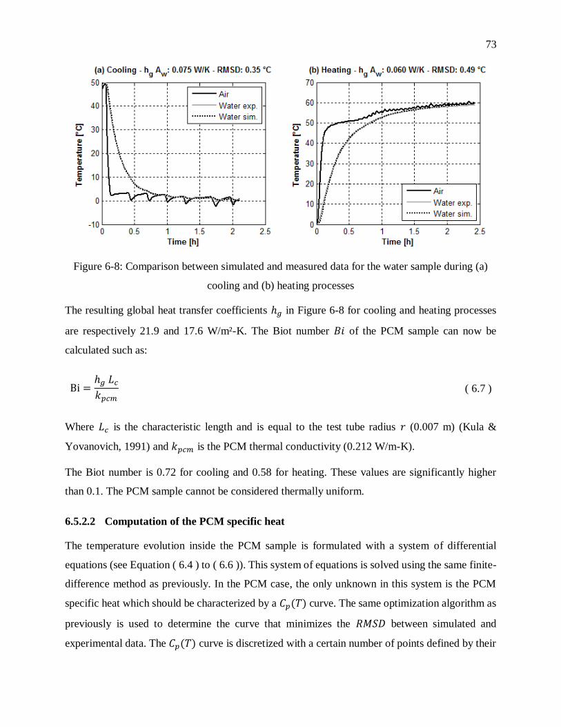
73
Figure 6-8: Comparison between simulated and measured data for the water sample during (a)
cooling and (b) heating processes
The resulting global heat transfer coefficients ℎ𝑔 in Figure 6-8 for cooling and heating processes
are respectively 21.9 and 17.6 W/m²-K. The Biot number 𝐵𝑖 of the PCM sample can now be
calculated such as:
Bi =ℎ𝑔 𝐿𝑐𝑘𝑝𝑐𝑚
( 6.7 )
Where 𝐿𝑐 is the characteristic length and is equal to the test tube radius 𝑟 (0.007 m) (Kula &
Yovanovich, 1991) and 𝑘𝑝𝑐𝑚 is the PCM thermal conductivity (0.212 W/m-K).
The Biot number is 0.72 for cooling and 0.58 for heating. These values are significantly higher
than 0.1. The PCM sample cannot be considered thermally uniform.
6.5.2.2 Computation of the PCM specific heat
The temperature evolution inside the PCM sample is formulated with a system of differential
equations (see Equation ( 6.4 ) to ( 6.6 )). This system of equations is solved using the same finite-
difference method as previously. In the PCM case, the only unknown in this system is the PCM
specific heat which should be characterized by a 𝐶𝑝(𝑇) curve. The same optimization algorithm as
previously is used to determine the curve that minimizes the 𝑅𝑀𝑆𝐷 between simulated and
experimental data. The 𝐶𝑝(𝑇) curve is discretized with a certain number of points defined by their
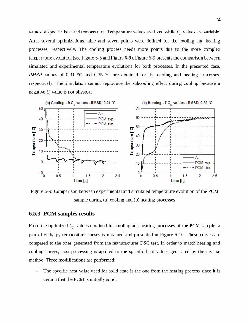
74
values of specific heat and temperature. Temperature values are fixed while 𝐶𝑝 values are variable.
After several optimizations, nine and seven points were defined for the cooling and heating
processes, respectively. The cooling process needs more points due to the more complex
temperature evolution (see Figure 6-5 and Figure 6-9). Figure 6-9 presents the comparison between
simulated and experimental temperature evolutions for both processes. In the presented case,
𝑅𝑀𝑆𝐷 values of 0.31 °C and 0.35 °C are obtained for the cooling and heating processes,
respectively. The simulation cannot reproduce the subcooling effect during cooling because a
negative 𝐶𝑝value is not physical.
Figure 6-9: Comparison between experimental and simulated temperature evolution of the PCM
sample during (a) cooling and (b) heating processes
6.5.3 PCM samples results
From the optimized 𝐶𝑝 values obtained for cooling and heating processes of the PCM sample, a
pair of enthalpy-temperature curves is obtained and presented in Figure 6-10. These curves are
compared to the ones generated from the manufacturer DSC test. In order to match heating and
cooling curves, post-processing is applied to the specific heat values generated by the inverse
method. Three modifications are performed:
- The specific heat value used for solid state is the one from the heating process since it is
certain that the PCM is initially solid.

75
- The specific heat value used for liquid state is the one from the cooling process since it is
certain that the PCM is initially liquid.
- The latent heat value used is the average of both cooling and heating processes.
Figure 6-10: Comparison between the enthalpy-temperature curves of the inverse method (IM)
and the DSC test
Figure 6-10 shows that the thermal capacity computed with the inverse method (IM) presented in
dotted lines is slightly lower. The latent heat obtained with the inverse method is nearly equivalent
to the value given by the DSC test (around 200 J/g). The curve slope during the solid state is slightly
lower with the inverse method, meaning that the specific heat (solid) has a lower value. On the
other hand, the specific heat for the liquid state shows no significant difference with the DSC value.
The inverse method shows a larger phase-change temperature range than the DSC test (especially
for cooling). This larger range is also observable on the temperature profiles shown in Figure 6-5.
These discrepancies can be attributed to different test conditions such as the applied heating and
cooling rates but also to sample size. The DSC tests have a rate of 2 °C/min and samples of a few
milligrams while the inverse method has a rate of around 0.8 °C/min and samples of approximately
10 grams.
6.6 Experimental results obtained with PCM-equipped walls
This section presents the experimental setup, the inverse method and the main results related to the
PCM-equipped walls.
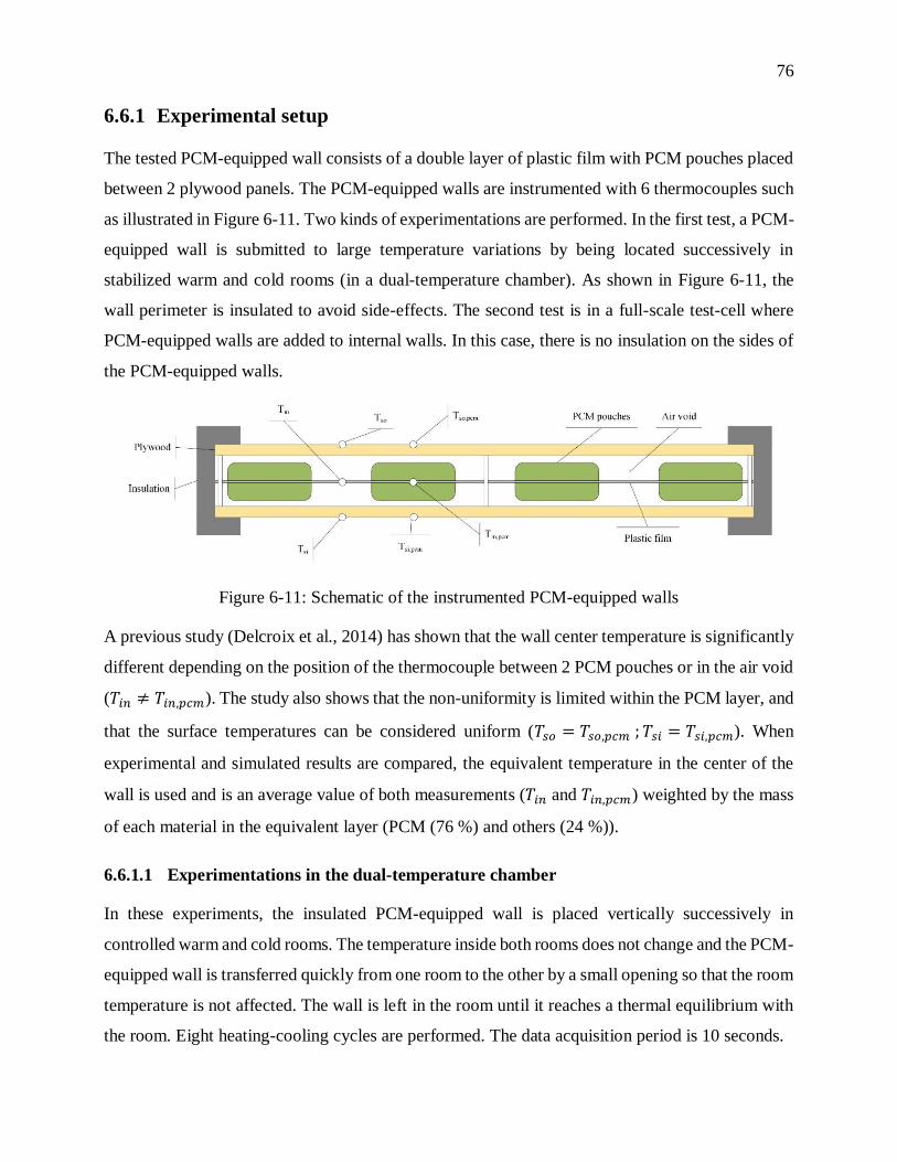
76
6.6.1 Experimental setup
The tested PCM-equipped wall consists of a double layer of plastic film with PCM pouches placed
between 2 plywood panels. The PCM-equipped walls are instrumented with 6 thermocouples such
as illustrated in Figure 6-11. Two kinds of experimentations are performed. In the first test, a PCM-
equipped wall is submitted to large temperature variations by being located successively in
stabilized warm and cold rooms (in a dual-temperature chamber). As shown in Figure 6-11, the
wall perimeter is insulated to avoid side-effects. The second test is in a full-scale test-cell where
PCM-equipped walls are added to internal walls. In this case, there is no insulation on the sides of
the PCM-equipped walls.
Figure 6-11: Schematic of the instrumented PCM-equipped walls
A previous study (Delcroix et al., 2014) has shown that the wall center temperature is significantly
different depending on the position of the thermocouple between 2 PCM pouches or in the air void
(𝑇𝑖𝑛 ≠ 𝑇𝑖𝑛,𝑝𝑐𝑚). The study also shows that the non-uniformity is limited within the PCM layer, and
that the surface temperatures can be considered uniform (𝑇𝑠𝑜 = 𝑇𝑠𝑜,𝑝𝑐𝑚 ; 𝑇𝑠𝑖 = 𝑇𝑠𝑖,𝑝𝑐𝑚). When
experimental and simulated results are compared, the equivalent temperature in the center of the
wall is used and is an average value of both measurements (𝑇𝑖𝑛 and 𝑇𝑖𝑛,𝑝𝑐𝑚) weighted by the mass
of each material in the equivalent layer (PCM (76 %) and others (24 %)).
6.6.1.1 Experimentations in the dual-temperature chamber
In these experiments, the insulated PCM-equipped wall is placed vertically successively in
controlled warm and cold rooms. The temperature inside both rooms does not change and the PCM-
equipped wall is transferred quickly from one room to the other by a small opening so that the room
temperature is not affected. The wall is left in the room until it reaches a thermal equilibrium with
the room. Eight heating-cooling cycles are performed. The data acquisition period is 10 seconds.

77
Figure 6-12 presents results for a cooling-heating cycle. Solid lines with circles show the
temperature evolutions of the PCM (𝑇𝑖𝑛,𝑝𝑐𝑚 in Figure 6-11) and in the air void (𝑇𝑖𝑛 in Figure 6-11).
Solid lines (S1 and S2) are surface temperatures. The dotted lines in grey and black present the
temperature evolutions for the air room and the equivalent layer (mass-weighted average of the
temperatures presented by solid lines with circles), respectively.
Figure 6-12: Experimental data for a cooling-heating cycle in the dual temperature chamber
Both graphs show that the phase change temperature range during cooling and heating is different.
The range is between 13 °C and 19 °C during cooling and between 17 °C and 21 °C during heating
if the black solid lines with circles are considered. It means that there is an important hysteresis
effect in these test conditions. If the average phase change temperatures are considered for cooling
(16 °C) and heating (19 °C), the hysteresis is around 3 °C. These graphs also show that cooling is
faster than heating. This can be explained by the higher convection coefficient in the cold zone of
the dual-temperature chamber, which has a higher ventilation rate.
6.6.1.2 Experimentations in the test-cell
The full-scale test-cell is fitted with instrumented PCM-equipped walls, which are added on the
inside surface of the north-west and south-west external walls (see Figure 6-13). Results are
presented for an extreme set-back scenario with a temperature set-point changing from 5 to 30 °C
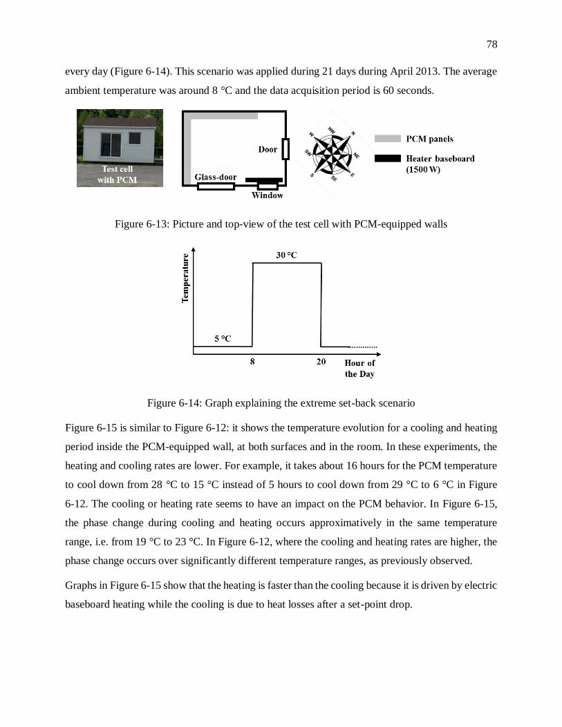
78
every day (Figure 6-14). This scenario was applied during 21 days during April 2013. The average
ambient temperature was around 8 °C and the data acquisition period is 60 seconds.
Figure 6-13: Picture and top-view of the test cell with PCM-equipped walls
Figure 6-14: Graph explaining the extreme set-back scenario
Figure 6-15 is similar to Figure 6-12: it shows the temperature evolution for a cooling and heating
period inside the PCM-equipped wall, at both surfaces and in the room. In these experiments, the
heating and cooling rates are lower. For example, it takes about 16 hours for the PCM temperature
to cool down from 28 °C to 15 °C instead of 5 hours to cool down from 29 °C to 6 °C in Figure
6-12. The cooling or heating rate seems to have an impact on the PCM behavior. In Figure 6-15,
the phase change during cooling and heating occurs approximatively in the same temperature
range, i.e. from 19 °C to 23 °C. In Figure 6-12, where the cooling and heating rates are higher, the
phase change occurs over significantly different temperature ranges, as previously observed.
Graphs in Figure 6-15 show that the heating is faster than the cooling because it is driven by electric
baseboard heating while the cooling is due to heat losses after a set-point drop.

79
Figure 6-15: Experimental data for a cooling-heating cycle in the test-cell
6.6.2 Inverse method applied to PCM-equipped walls experimentations
The PCM-equipped wall is represented as an R-C model (Figure 6-16) with 30 nodes whose
boundary conditions are the surface temperatures. The properties (Table 6-3) of the central
equivalent layer consist in combined properties of each material, i.e. PCM, plastic film and air. The
density is the volumetric average of the densities. The equivalent thermal conductivity is estimated
using THERM (Lawrence Berkeley National Laboratory, 2013). The air thermal resistance was
determined by assuming a thermal conductivity of 0.026 W/m-K and a radiative heat transfer
computed from Kirchhoff’s law (Spakovszki, 2014). As the air layer is very thin, the convective
heat transfer is assumed to be negligible. The equivalent specific heat 𝐶𝑝(𝑇) is determined through
the inverse method. First, the equivalent values of latent heat and specific heat for solid and liquid
states (Table 6-4) can be calculated from known thermal capacity values and the mass fraction of
each material in the equivalent layer. Then the phase change temperature range is determined by
the inverse method. The central node inside the equivalent layer is the one used to match simulated
and experimental data. The objective function shown in Equation ( 6.2 ) is used.

80
Figure 6-16: Modeling of the PCM-equipped wall
Table 6-3: Properties of the model for the PCM-equipped wall
Layer Thickness
[m]
Thermal conductivity
[W/m-K]
Density
[kg/m³]
Specific heat
[J/g-K]
Plywood 0.006 0.084 850 1.25
Equivalent layer 0.017 0.042 223 N/A
Table 6-4: Thermal capacity definition of the equivalent layer
Material Mass
share [%]
Specific
heat [J/g-K]
Specific heat
(solid) [J/g-K]
Specific heat
(liquid) [J/g-K]
Latent
heat [J/g]
Air 0.4 1 N/A N/A N/A
Plastic film 23.5 1.5 N/A N/A N/A
PCM 76.1 N/A 1.84 1.99 200
Equivalent layer N/A N/A 1.76 1.87 150
For each node presented in Figure 6-16, the temperature variation over time is computed as follows:
𝑑𝑇𝑛𝑑𝑡
=𝑈𝑙,𝑛𝐶𝑛
(𝑇𝑛−1 − 𝑇𝑛) +𝑈𝑟,𝑛𝐶𝑛
(𝑇𝑛+1 − 𝑇𝑛) ( 6.8 )
Equation ( 6.8 ) is solved with a forward time and central space finite-difference method with a
time-step of 10 and 60 seconds, respectively for the dual-temperature chamber and test-cell
experimentations. The corresponding stability condition based on the Fourier number is met
(Bergman et al., 2011). In Equation ( 6.8 ), the only parameter that has to be determined for the
equivalent layer is the node capacitance 𝐶𝑛, which is equal to:
𝐶𝑛 = 𝜌𝑛 𝐶𝑝,𝑛 ∆𝑥𝑛 ( 6.9 )

81
The density 𝜌 and the node interval ∆𝑥 are constant. Only the temperature-dependent specific heat
𝐶𝑝(𝑇) is to be optimized and is defined using 2 variables (Figure 6-17). Two temperatures defining
the beginning (𝑇𝑜𝑛) and the end (𝑇𝑜𝑓𝑓) of the phase change are optimized. The three specific heat
values for solid (𝐶𝑝,𝑠), mushy (𝐶𝑝,𝑝𝑐) and liquid (𝐶𝑝,𝑙) states are set to the values in Table 6-4.
Figure 6-17: Graphs explaining the variables to be optimized during (a) cooling and (b) heating
processes
Optimizations are separately applied to 50 cooling cases (42 in the test-cell and 8 in the dual-
temperature chamber) and 48 heating cases (40 in the test-cell and 8 in the dual-temperature
chamber), which display varying degree of heating and cooling rates.
A case for both tests and processes is shown in Figure 6-18 and Figure 6-19, where simulated and
experimental results are in good agreement.
Figure 6-18: Comparison between experimental and simulated temperature evolution for wall
experimentations during (a) cooling and (b) heating processes
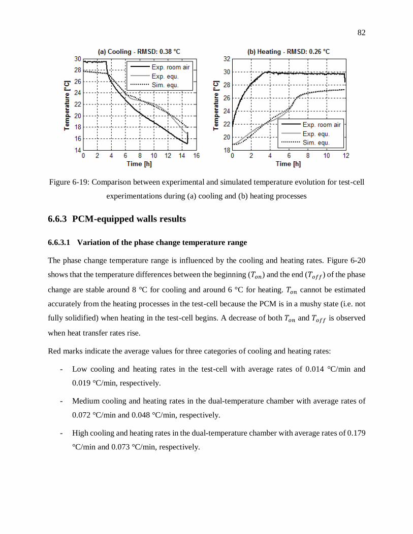
82
Figure 6-19: Comparison between experimental and simulated temperature evolution for test-cell
experimentations during (a) cooling and (b) heating processes
6.6.3 PCM-equipped walls results
6.6.3.1 Variation of the phase change temperature range
The phase change temperature range is influenced by the cooling and heating rates. Figure 6-20
shows that the temperature differences between the beginning (𝑇𝑜𝑛) and the end (𝑇𝑜𝑓𝑓) of the phase
change are stable around 8 °C for cooling and around 6 °C for heating. 𝑇𝑜𝑛 cannot be estimated
accurately from the heating processes in the test-cell because the PCM is in a mushy state (i.e. not
fully solidified) when heating in the test-cell begins. A decrease of both 𝑇𝑜𝑛 and 𝑇𝑜𝑓𝑓 is observed
when heat transfer rates rise.
Red marks indicate the average values for three categories of cooling and heating rates:
- Low cooling and heating rates in the test-cell with average rates of 0.014 °C/min and
0.019 °C/min, respectively.
- Medium cooling and heating rates in the dual-temperature chamber with average rates of
0.072 °C/min and 0.048 °C/min, respectively.
- High cooling and heating rates in the dual-temperature chamber with average rates of 0.179
°C/min and 0.073 °C/min, respectively.
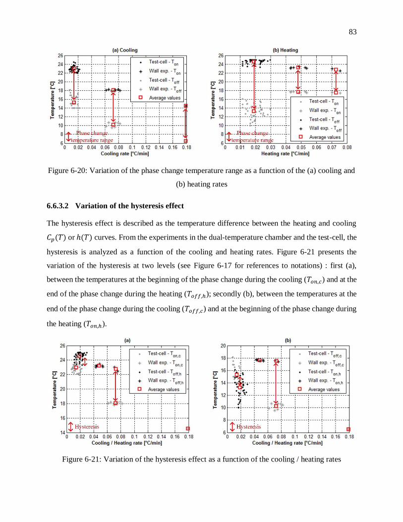
83
Figure 6-20: Variation of the phase change temperature range as a function of the (a) cooling and
(b) heating rates
6.6.3.2 Variation of the hysteresis effect
The hysteresis effect is described as the temperature difference between the heating and cooling
𝐶𝑝(𝑇) or ℎ(𝑇) curves. From the experiments in the dual-temperature chamber and the test-cell, the
hysteresis is analyzed as a function of the cooling and heating rates. Figure 6-21 presents the
variation of the hysteresis at two levels (see Figure 6-17 for references to notations) : first (a),
between the temperatures at the beginning of the phase change during the cooling (𝑇𝑜𝑛,𝑐) and at the
end of the phase change during the heating (𝑇𝑜𝑓𝑓,ℎ); secondly (b), between the temperatures at the
end of the phase change during the cooling (𝑇𝑜𝑓𝑓,𝑐) and at the beginning of the phase change during
the heating (𝑇𝑜𝑛,ℎ).
Figure 6-21: Variation of the hysteresis effect as a function of the cooling / heating rates
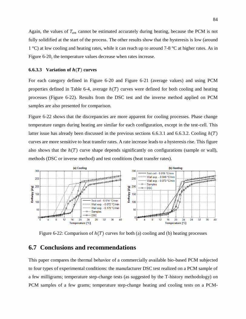
84
Again, the values of 𝑇𝑜𝑛 cannot be estimated accurately during heating, because the PCM is not
fully solidified at the start of the process. The other results show that the hysteresis is low (around
1 °C) at low cooling and heating rates, while it can reach up to around 7-8 °C at higher rates. As in
Figure 6-20, the temperature values decrease when rates increase.
6.6.3.3 Variation of 𝒉(𝑻) curves
For each category defined in Figure 6-20 and Figure 6-21 (average values) and using PCM
properties defined in Table 6-4, average ℎ(𝑇) curves were defined for both cooling and heating
processes (Figure 6-22). Results from the DSC test and the inverse method applied on PCM
samples are also presented for comparison.
Figure 6-22 shows that the discrepancies are more apparent for cooling processes. Phase change
temperature ranges during heating are similar for each configuration, except in the test-cell. This
latter issue has already been discussed in the previous sections 6.6.3.1 and 6.6.3.2. Cooling ℎ(𝑇)
curves are more sensitive to heat transfer rates. A rate increase leads to a hysteresis rise. This figure
also shows that the ℎ(𝑇) curve shape depends significantly on configurations (sample or wall),
methods (DSC or inverse method) and test conditions (heat transfer rates).
Figure 6-22: Comparison of ℎ(𝑇) curves for both (a) cooling and (b) heating processes
6.7 Conclusions and recommendations
This paper compares the thermal behavior of a commercially available bio-based PCM subjected
to four types of experimental conditions: the manufacturer DSC test realized on a PCM sample of
a few milligrams; temperature step-change tests (as suggested by the T-history methodology) on
PCM samples of a few grams; temperature step-change heating and cooling tests on a PCM-
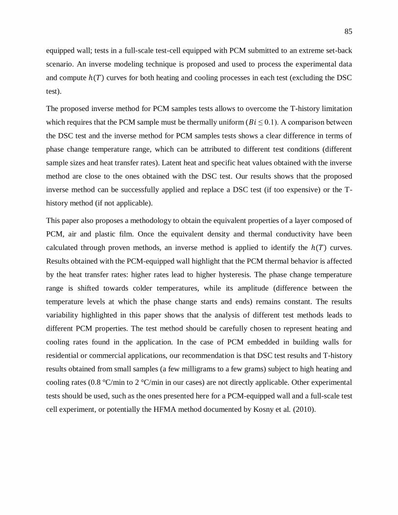
85
equipped wall; tests in a full-scale test-cell equipped with PCM submitted to an extreme set-back
scenario. An inverse modeling technique is proposed and used to process the experimental data
and compute ℎ(𝑇) curves for both heating and cooling processes in each test (excluding the DSC
test).
The proposed inverse method for PCM samples tests allows to overcome the T-history limitation
which requires that the PCM sample must be thermally uniform (𝐵𝑖 ≤ 0.1). A comparison between
the DSC test and the inverse method for PCM samples tests shows a clear difference in terms of
phase change temperature range, which can be attributed to different test conditions (different
sample sizes and heat transfer rates). Latent heat and specific heat values obtained with the inverse
method are close to the ones obtained with the DSC test. Our results shows that the proposed
inverse method can be successfully applied and replace a DSC test (if too expensive) or the T-
history method (if not applicable).
This paper also proposes a methodology to obtain the equivalent properties of a layer composed of
PCM, air and plastic film. Once the equivalent density and thermal conductivity have been
calculated through proven methods, an inverse method is applied to identify the ℎ(𝑇) curves.
Results obtained with the PCM-equipped wall highlight that the PCM thermal behavior is affected
by the heat transfer rates: higher rates lead to higher hysteresis. The phase change temperature
range is shifted towards colder temperatures, while its amplitude (difference between the
temperature levels at which the phase change starts and ends) remains constant. The results
variability highlighted in this paper shows that the analysis of different test methods leads to
different PCM properties. The test method should be carefully chosen to represent heating and
cooling rates found in the application. In the case of PCM embedded in building walls for
residential or commercial applications, our recommendation is that DSC test results and T-history
results obtained from small samples (a few milligrams to a few grams) subject to high heating and
cooling rates (0.8 °C/min to 2 °C/min in our cases) are not directly applicable. Other experimental
tests should be used, such as the ones presented here for a PCM-equipped wall and a full-scale test
cell experiment, or potentially the HFMA method documented by Kosny et al. (2010).
86
Acknowledgements
The research work presented in this paper is financially supported by Hydro-Québec, FRQNT
(Fonds de Recherche du Québec en Nature et Technologies) and NSERC (Natural Sciences and
Engineering Research Council of Canada).
References
Atchonouglo, K., Banna, M., Vallée, C., & Dupré, J.-C. (2008). Inverse transient heat conduction
problems and identification of thermal parameters. Heat and Mass Transfer, 45(1), 23–29.
doi:10.1007/s00231-008-0383-7
Baetens, R., Jelle, B. P., & Gustavsen, A. (2010). Phase change materials for building
applications: A state-of-the-art review. Energy and Buildings, 42(9), 1361–1368.
doi:http://dx.doi.org/10.1016/j.enbuild.2010.03.026
Bergman, T. L., Lavine, A. S., Incropera, F. P., & Dewitt, D. P. (2011). Fundamentals of heat and
mass transfer. Wiley.
Braun, J. E., & Chaturvedi, N. (2002). An Inverse Gray-Box Model for Transient Building Load
Prediction. HVAC&R Research, 8(1), 73–99. Retrieved from
http://www.tandfonline.com/doi/abs/10.1080/10789669.2002.10391290
Castell, A., Medrano, M., Castellón, C., & Cabeza, L. F. (2009). Analysis of the simulation
models for the use of PCM in buildings. In Effstock: Thermal Energy Storage for Efficiency
and Sustainability. Stockholm.
Cheng, R., Pomianowski, M., Wang, X., Heiselberg, P., & Zhang, Y. (2013). A new method to
determine thermophysical properties of PCM-concrete brick. Applied Energy, 112, 988–
998. doi:10.1016/j.apenergy.2013.01.046
Crawley, D. B., Lawrie, L. K., Winkelmann, F. C., Buhl, W. F., Huang, Y. J., Pedersen, C. O.,
Strand, R. K., Liesen, R. J., Fischer, D. E., Witte, M. J., Glazer, J. (2001). EnergyPlus:

87
creating a new-generation building energy simulation program. Energy and Buildings, 33(4),
319–331. doi:http://dx.doi.org/10.1016/S0378-7788(00)00114-6
Delcroix, B., Kummert, M., Daoud, A., & Bouchard, J. (2014). Experimental assessment of a
phase change material in walls for heating and cooling applications. In eSim (pp. 1 – 13).
Ottawa, ON, Canada.
Dentel, A., & Stephan, W. (2010). Thermal Comfort in Rooms with active PCM Constructions.
In 8th International Conference on System Simulation in Buildings (pp. 1–16). Liège,
Belgium.
Energy Systems Research Unit. (1998). ESP-r User Guide: The ESP-r System for Building
Energy Simulation. Glasgow.
German Institute for Quality Assurance and Certification. (2009). Phase change material. Berlin,
Germany.
Goodrich, L. E. (1978). Efficient numerical technique for one-dimensional thermal problems with
phase-change. International Journal of Heat and Mass Transfer, 21(5), 615.
Günther, E., Hiebler, S., Mehling, H., & Redlich, R. (2009). Enthalpy of Phase Change Materials
as a Function of Temperature: Required Accuracy and Suitable Measurement Methods.
International Journal of Thermophysics, 30(4), 1257.
Günther, E., Mehling, H., & Hiebler, S. (2007). Modeling of subcooling and solidification of
phase change materials. Modelling and Simulation in Materials Science and Engineering,
15, 879–892. doi:10.1088/0965-0393/15/8/005
Heim, D., & Clarke, J. A. (2004). Numerical modelling and thermal simulation of PCM–gypsum
composites with ESP-r. Energy and Buildings, 36, 795–805.
doi:10.1016/j.enbuild.2004.01.004
88
Huang, C.-H., & Jan-Yuan, Y. (1995). An inverse problem in simultaneously measuring
temperature-dependent thermal conductivity and heat capacity. International Journal of Heat
and Mass Transfer, 38(18), 3433–3441. doi:10.1016/0017-9310(95)00059-I
Ibánez, M., Lázaro, A., Zalba, B., & Cabeza, L. F. (2005). An approach to the simulation of
PCMs in building applications using TRNSYS. Applied Thermal Engineering, 25, 1796–
1807.
Klein, S. A., Beckman, W. A., Mitchell, J. W., Duffie, J. A., Duffie, N. A., & Freeman, T. L.
(2012). TRNSYS 17: A Transient System Simulation Program. Madison, USA: Solar
Energy Laboratory, University of Wisconsin. Retrieved from http://sel.me.wisc.edu/trnsys
Kosny, J., Stovall, T., Shrestha, S., & Yarbrough, D. (2010). Theoretical and Experimental
Thermal Performance Analysis of Complex Thermal Storage Membrane Containing Bio-
Based Phase-Change Material (PCM). In Building XI (p. 11).
Kula, L. W., & Yovanovich, M. M. (1991). Characteristic length of complex bodies for transient
conduction. ASME Thermal Engineering Proceedings, 1, 259–267.
Kuznik, F., & Virgone, J. (2009). Experimental investigation of wallboard containing phase
change material: Data for validation of numerical modeling. Energy and Buildings, 41(5),
561–570. doi:10.1016/j.enbuild.2008.11.022
Kuznik, F., Virgone, J., & Johannes, K. (2010). Development and validation of a new TRNSYS
type for the simulation of external building walls containing PCM. Energy and Buildings,
42, 1004–1009.
Lawrence Berkeley National Laboratory. (2013). THERM 6.3 / WINDOW 6.3 - NFRC
Simulation Manual.
Mehling, H., & Cabeza, L. F. (2008). Heat and cold storage with PCM: An up to date
introduction into basics and applications. (D. Mewes & F. Mayinger, Eds.). Berlin: Springer.

89
Pedersen, C. O. (2007). Advanced zone simulation in EnergyPlus: incorporation of variable
properties and phase change material (PCM) capability. In Building Simulation (pp. 1341–
1345). Beijing.
Phase change energy solutions. (2008). BioPCM longevity cycle testing. Retrieved from
http://www.phasechange.com/index.php/en/contractor-library
Poulad, M. E., Fung, A. S., & Naylor, D. (2011). Effects of convective heat transfer coefficient
on the ability of PCM to reduce building energy demand. In 12th Conference of
International Building Performance Simulation Association (pp. 270–277). Sydney.
Recktenwald, G. W. (2011). Finite-Difference Approximations to the Heat Equation (Vol. 0).
Portland, Oregon, USA. Retrieved from http://www.f.kth.se/~jjalap/numme/FDheat.pdf
Schranzhofer, H., Puschnig, P., Heinz, A., & Streicher, W. (2006). Validation of a TRNSYS
simulation model for PCM energy storages and PCM wall construction elements. In 10th
International Conference on Thermal Energy Storage. New Jersey.
Sharma, A., Tyagi, V. V, Chen, C. R., & Buddhi, D. (2009). Review on thermal energy storage
with phase change materials and applications. Renewable and Sustainable Energy Reviews,
13(2), 318–345. doi:http://dx.doi.org/10.1016/j.rser.2007.10.005
Shrestha, S., Miller, W., Stovall, T., Desjarlais, A., Childs, K., Porter, W., Bhandary, M., Coley,
S. (2011). Modeling PCM-enhanced insulation system and benchmarking EnergyPlus
against controlled field data. In 12th Conference of International Building Performance
Simulation Association (pp. 800–807). Sydney.
Solé, A., Miró, L., Barreneche, C., Martorell, I., & Cabeza, L. F. (2013). Review of the T-history
method to determine thermophysical properties of phase change materials (PCM).
Renewable and Sustainable Energy Reviews, 26, 425–436. doi:10.1016/j.rser.2013.05.066
Spakovszki, Z. S. (2014). 19.3 Radiation heat transfer between planar surfaces. Retrieved
February 25, 2015, from
http://web.mit.edu/16.unified/www/FALL/thermodynamics/notes/node136.html
90
Tabares-Velasco, P. C., Christensen, C., & Bianchi, M. (2012). Verification and validation of
EnergyPlus phase change material model for opaque wall assemblies. Building and
Environment, 54, 186–196.
The MathWorks Inc. (2014). GA - Find minimum of function using genetic algorithm. Retrieved
July 2, 2014, from http://www.mathworks.com/help/gads/ga.html
Voller, V. R., & Cross, M. (1981). Accurate solutions of moving boundary problems using the
enthalpy method. International Journal of Heat and Mass Transfer, 24(3), 545.
Yao, M., & Chait, A. (1993). An alternative formulation of the apparent heat capacity method for
phase change problems. Numerical Heat Transfer, Part B, Fundamentals, 24(3), 279.
Zalba, B., Marın, J. M., Cabeza, L. F., & Mehling, H. (2003). Review on thermal energy storage
with phase change: materials, heat transfer analysis and applications. Applied Thermal
Engineering, 23(3), 251–283. doi:http://dx.doi.org/10.1016/S1359-4311(02)00192-8

91
CHAPTER 7 ARTICLE 3: THERMAL BEHAVIOR MAPPING OF A
PHASE CHANGE MATERIAL BETWEEN THE HEATING AND
COOLING ENTHALPY-TEMPERATURE CURVES
Delcroix, B., Kummert, M., Daoud, A., (2015). Thermal behavior mapping of a phase change
material between the heating and cooling enthalpy-temperature curves. 6th International Building
Physics Conference. Torino, Italy.
Abstract
This paper presents the results of experimental tests performed on a wall section equipped with
phase change materials (PCM). The wall is quickly transferred between cold and warm enclosures
to observe the PCM behavior when melting or solidification is interrupted. A 1-D model of the
wall based on the enthalpy method is used to identify the enthalpy curves that provide the best fit
to experimental data. Results show that the PCM experiences a quick transition between different
enthalpy curves when the heat flow direction (heating or cooling) is reversed during phase-change.
According to our experiments and to the comparison with the 1-D model, the PCM investigated
here follows an enthalpy curve that is very close to the heating curve when a cooling process is
interrupted during solidification. If a heating process is interrupted during melting, the PCM
follows an enthalpy curve that is located between the heating and cooling curves. This information
is important to develop models for PCM used in buildings and further work is required to assess
the impact of different factors on the transitional behavior.
Nomenclature
𝐴 Area [m²]
Bi Biot number [-]
Fo Fourier number [-]
ℎ Enthalpy [J/g]
𝑖 Node [-]
𝑙 Left [-]

92
𝑚 Mass [g]
𝑛 Number of nodes [-]
𝑟 Right [-]
𝑇 Temperature [°C]
𝑈 Heat transfer coefficient [W/m²-K]
𝑡 Time [s]
7.1 Introduction
Using phase change materials (PCM) to increase the building thermal mass is a possible solution
for peak shaving and shifting of heating and cooling loads (Farid, Khudhair, Razack, & Al-Hallaj,
2004; Sharma et al., 2009). Recent efforts focus on developing models (Al-Saadi & Zhai, 2013;
Dutil, Rousse, Salah, Lassue, & Zalewski, 2011) which generally rely on enthalpy-temperature
curve(s) which define the PCM thermal behavior during heating and cooling processes. The PCM
behavior during its two-phase state (liquid-solid state) remains uncertain. For example, if a PCM
is cooled down after a partial melting, different scenarios are possible, as shown in Figure 7-1. A
first scenario suggested by Bony and Citherlet (2007) is a transition to the cooling curve using a
slope equivalent to the solid or liquid specific heat (wT). Chandrasekharan et al. (2013) have
suggested a second option (noT) which consists in staying on the heating curve.
Figure 7-1: Possible behavior of a PCM cooled down after partial melting
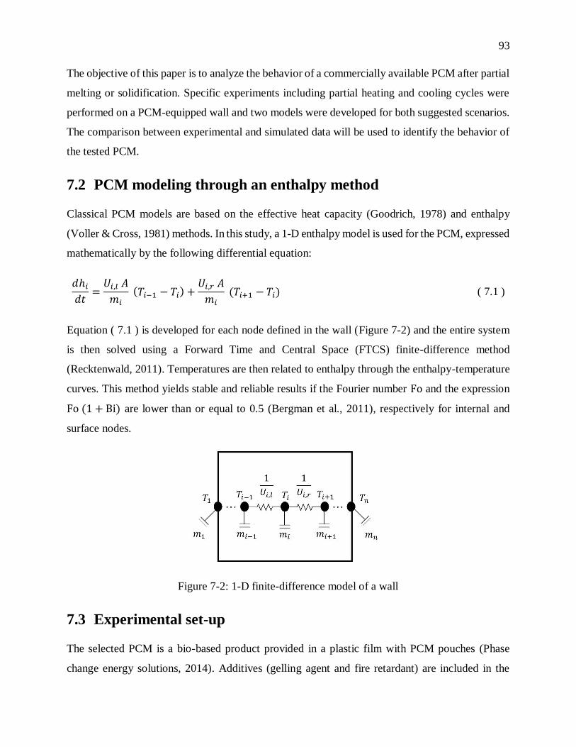
93
The objective of this paper is to analyze the behavior of a commercially available PCM after partial
melting or solidification. Specific experiments including partial heating and cooling cycles were
performed on a PCM-equipped wall and two models were developed for both suggested scenarios.
The comparison between experimental and simulated data will be used to identify the behavior of
the tested PCM.
7.2 PCM modeling through an enthalpy method
Classical PCM models are based on the effective heat capacity (Goodrich, 1978) and enthalpy
(Voller & Cross, 1981) methods. In this study, a 1-D enthalpy model is used for the PCM, expressed
mathematically by the following differential equation:
𝑑ℎ𝑖𝑑𝑡
=𝑈𝑖,𝑙 𝐴
𝑚𝑖 (𝑇𝑖−1 − 𝑇𝑖) +
𝑈𝑖,𝑟 𝐴
𝑚𝑖 (𝑇𝑖+1 − 𝑇𝑖) ( 7.1 )
Equation ( 7.1 ) is developed for each node defined in the wall (Figure 7-2) and the entire system
is then solved using a Forward Time and Central Space (FTCS) finite-difference method
(Recktenwald, 2011). Temperatures are then related to enthalpy through the enthalpy-temperature
curves. This method yields stable and reliable results if the Fourier number Fo and the expression
Fo (1 + Bi) are lower than or equal to 0.5 (Bergman et al., 2011), respectively for internal and
surface nodes.
Figure 7-2: 1-D finite-difference model of a wall
7.3 Experimental set-up
The selected PCM is a bio-based product provided in a plastic film with PCM pouches (Phase
change energy solutions, 2014). Additives (gelling agent and fire retardant) are included in the

94
product. Manufacturer data (Phase change energy solutions, 2014) on the PCM includes some
properties for the pure PCM and some for the final product with additives. Table 7-1 summarizes
the available data. The density and the thermal conductivity for the PCM with additives have been
obtained through additional experimentations.
Table 7-1: PCM properties
Without additives With additives
Phase change temperature °C 23 Phase change
temperature °C 23
Latent heat storage capacity J/g 203 Latent heat storage
capacity J/g
165-
200 Density kg/m³ 830
Specific heat (solid) J/g-K 1.84 Weight per unit surface kg/m² 1.465
Specific heat (liquid) J/g-K 1.99 Density kg/m³ 883 *
Thermal conductivity (solid) W/m-K 0.207 Thermal conductivity
(solid and liquid)
W/m-
K 0.212 ^
Thermal conductivity (liquid) W/m-K 0.171
* Experimental measurements (standard deviation: ± 10 kg/m³) – not from manufacturer
^ Experimental measurements (standard deviation: ± 0.022 W/m-K) – not from manufacturer
The tested wall consists of a double layer of plastic film with PCM pouches, sandwiched between
two plywood boards. The wall has an area of 0.6 m² (1 m x 0.6 m) and is instrumented with
thermocouples (accuracy: ± 0.5 °C) (Figure 7-3). The wall perimeter is insulated to avoid side-
effects. The central layer composed of PCM, plastic film and air is modeled as an equivalent 1-D
layer (Figure 7-4 (a)). The main properties of the wall are given in Table 7-2. Figure 7-4 (b) presents
the enthalpy-temperature curves of the equivalent layer obtained from a model calibration
performed on experimental data with complete heating/cooling cycles. Figure 7-4 (a) also shows
the temperature values that are further presented and compared to experimental data. 𝑇𝑃𝐶𝑀 is
compared to the mean value of 𝑇𝑖𝑛,𝑝𝑐𝑚 and 𝑇𝑖𝑛 (Figure 7-3) weighted by the mass of each material
in the equivalent layer (PCM (76 %) and others (24 %)). 𝑇𝑠𝑖 is compared to the mean value of 𝑇𝑠𝑖,1
and 𝑇𝑠𝑖,2. The same method as 𝑇𝑠𝑖 is applied for 𝑇𝑠𝑜.

95
Figure 7-3: Instrumented PCM-equipped wall
Table 7-2: Layers properties
Layer Thickness
[m]
Thermal conductivity
[W/m-K]
Density
[kg/m³]
Specific heat
[J/g-K]
Plywood 0.006 0.084 850 1.25
Equivalent layer 0.017 0.042* 223 See Figure 7-4 (b)
* Using THERM (Lawrence Berkeley National Laboratory, 2013)
Figure 7-4: (a) PCM-equipped wall model; (b) Enthalpy-temperature curves of the
equivalent layer
7.4 Results
7.4.1 Experimental data
Two series of experiments were performed on one PCM-equipped wall. Figure 7-5 (a) presents the
interrupted heating scenario where the PCM-equipped wall, initially at a uniform cold temperature,
is heated up by quickly transferring the wall into a warmer environment, until the PCM starts
melting. Before the end of the phase change, the wall is quickly transferred back into the colder
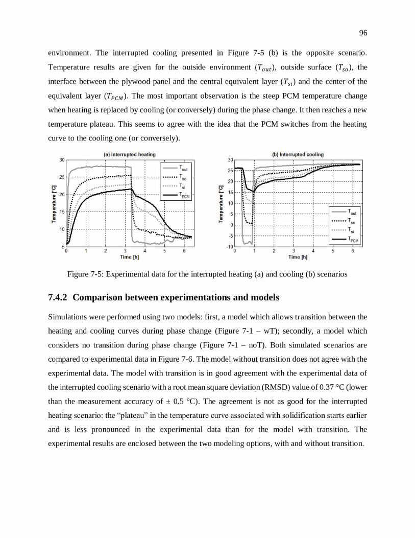
96
environment. The interrupted cooling presented in Figure 7-5 (b) is the opposite scenario.
Temperature results are given for the outside environment (𝑇𝑜𝑢𝑡), outside surface (𝑇𝑠𝑜), the
interface between the plywood panel and the central equivalent layer (𝑇𝑠𝑖) and the center of the
equivalent layer (𝑇𝑃𝐶𝑀). The most important observation is the steep PCM temperature change
when heating is replaced by cooling (or conversely) during the phase change. It then reaches a new
temperature plateau. This seems to agree with the idea that the PCM switches from the heating
curve to the cooling one (or conversely).
Figure 7-5: Experimental data for the interrupted heating (a) and cooling (b) scenarios
7.4.2 Comparison between experimentations and models
Simulations were performed using two models: first, a model which allows transition between the
heating and cooling curves during phase change (Figure 7-1 – wT); secondly, a model which
considers no transition during phase change (Figure 7-1 – noT). Both simulated scenarios are
compared to experimental data in Figure 7-6. The model without transition does not agree with the
experimental data. The model with transition is in good agreement with the experimental data of
the interrupted cooling scenario with a root mean square deviation (RMSD) value of 0.37 °C (lower
than the measurement accuracy of ± 0.5 °C). The agreement is not as good for the interrupted
heating scenario: the “plateau” in the temperature curve associated with solidification starts earlier
and is less pronounced in the experimental data than for the model with transition. The
experimental results are enclosed between the two modeling options, with and without transition.

97
Figure 7-6: Comparison between experimental and simulated data for the interrupted heating (a)
and cooling (b) scenarios
7.4.3 Mapping of a solution
An optimization algorithm was used in order to find the enthalpy-temperature curves that match
the experimental and simulated data for both tests. The resulting temperature profiles are presented
in Figure 7-7; they show a good agreement with experimental data, with RMSD values of 0.64 °C
and 0.28 °C, respectively for the interrupted heating and cooling scenarios. Both values are close
to the measurement accuracy of ± 0.5 °C.
Figure 7-7: Comparison between experimental and optimized simulated data for the interrupted
heating (a) and cooling (b) scenarios
Figure 7-8 shows the path followed by the PCM on the enthalpy-temperature curves for both
scenarios according to the optimization results. Initial curves (solid lines) from Figure 7-4 (b) are
preserved while the optimized curve (dotted lines) followed by the PCM after the transition is also
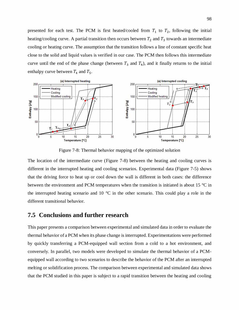
98
presented for each test. The PCM is first heated/cooled from 𝑇1 to 𝑇2, following the initial
heating/cooling curve. A partial transition then occurs between 𝑇2 and 𝑇3 towards an intermediate
cooling or heating curve. The assumption that the transition follows a line of constant specific heat
close to the solid and liquid values is verified in our case. The PCM then follows this intermediate
curve until the end of the phase change (between 𝑇3 and 𝑇4), and it finally returns to the initial
enthalpy curve between 𝑇4 and 𝑇5.
Figure 7-8: Thermal behavior mapping of the optimized solution
The location of the intermediate curve (Figure 7-8) between the heating and cooling curves is
different in the interrupted heating and cooling scenarios. Experimental data (Figure 7-5) shows
that the driving force to heat up or cool down the wall is different in both cases: the difference
between the environment and PCM temperatures when the transition is initiated is about 15 °C in
the interrupted heating scenario and 10 °C in the other scenario. This could play a role in the
different transitional behavior.
7.5 Conclusions and further research
This paper presents a comparison between experimental and simulated data in order to evaluate the
thermal behavior of a PCM when its phase change is interrupted. Experimentations were performed
by quickly transferring a PCM-equipped wall section from a cold to a hot environment, and
conversely. In parallel, two models were developed to simulate the thermal behavior of a PCM-
equipped wall according to two scenarios to describe the behavior of the PCM after an interrupted
melting or solidification process. The comparison between experimental and simulated data shows
that the PCM studied in this paper is subject to a rapid transition between the heating and cooling
99
curves if the heating or cooling process is interrupted during phase change. For the interrupted
heating process, the transition is partial and the PCM follows an enthalpy curve which is located
between the heating and cooling curves. Further research will aim at assessing the impact of
different factors such as the heat transfer rate on the transitional behavior.
References
Al-Saadi, S. N., & Zhai, Z. (John). (2013). Modeling phase change materials embedded in
building enclosure: A review. Renewable and Sustainable Energy Reviews, 21, 659–673.
doi:10.1016/j.rser.2013.01.024
Bergman, T. L., Lavine, A. S., Incropera, F. P., & Dewitt, D. P. (2011). Fundamentals of heat and
mass transfer. Wiley.
Bony, J., & Citherlet, S. (2007). Numerical model and experimental validation of heat storage
with phase change materials. Energy and Buildings, 39, 1065–1072. Retrieved from
http://www.sciencedirect.com/science/article/pii/S037877880600291X
Chandrasekharan, R., Lee, E. S., Fisher, D. E., & Deokar, P. S. (2013). An Enhanced Simulation
Model for Building Envelopes with Phase Change Materials. ASHRAE Transactions,
119(2).
Dutil, Y., Rousse, D. R., Salah, N. Ben, Lassue, S., & Zalewski, L. (2011). A review on phase-
change materials: Mathematical modeling and simulations. Renewable and Sustainable
Energy Reviews, 15, 112–130. Retrieved from
http://www.sciencedirect.com/science/article/pii/S1364032110001589
Farid, M. M., Khudhair, A. M., Razack, S. A. K., & Al-Hallaj, S. (2004). A review on phase
change energy storage: materials and applications. Energy Conversion and Management,
45(9–10), 1597–1615. doi:http://dx.doi.org/10.1016/j.enconman.2003.09.015
Goodrich, L. E. (1978). Efficient numerical technique for one-dimensional thermal problems with
phase-change. International Journal of Heat and Mass Transfer, 21(5), 615.

100
Lawrence Berkeley National Laboratory. (2013). THERM 6.3 / WINDOW 6.3 - NFRC
Simulation Manual.
Phase change energy solutions. (2014). Manufacturing innovative thermal storage technologies
for smart & sustainable buildings. Retrieved February 9, 2015, from
http://www.phasechange.com/index.php
Recktenwald, G. W. (2011). Finite-Difference Approximations to the Heat Equation (Vol. 0).
Portland, Oregon, USA. Retrieved from http://www.f.kth.se/~jjalap/numme/FDheat.pdf
Sharma, A., Tyagi, V. V, Chen, C. R., & Buddhi, D. (2009). Review on thermal energy storage
with phase change materials and applications. Renewable and Sustainable Energy Reviews,
13(2), 318–345. doi:http://dx.doi.org/10.1016/j.rser.2007.10.005
Voller, V., & Cross, M. (1981). Accurate solutions of moving boundary problems using the
enthalpy method. International Journal of Heat and Mass Transfer, 24(3), 545.
101
CHAPTER 8 ARTICLE 4: MODELING OF A WALL WITH PHASE
CHANGE MATERIALS. PART I: DEVELOPMENT AND NUMERICAL
VALIDATION
Delcroix, B., Kummert, M., Daoud, A., (2015). Modeling of a wall with phase change materials.
Part I: Development and numerical validation. Submitted to Journal of Building Performance
Simulation on the 15th of July 2015.
Abstract
This paper presents a new TRNSYS model of a wall with variable properties, named Type 3258
and dedicated to modeling phase change materials (PCMs) in the building envelope. The 1-D
conduction heat transfer equation is solved using an explicit finite-difference method coupled with
an enthalpy method to take into account the variable PCM thermal capacity. This model includes
temperature-dependent thermal conductivity as well as PCM-specific effects such as hysteresis and
subcooling. The stability conditions are discussed and the algorithm implemented in TRNSYS is
described. A numerical validation performed on wall test cases proposed by the International
Energy Agency (Annex 23) is presented, showing that the developed model is in agreement with
reference models. The paper also discusses the impact of temporal and spatial discretization on the
model performance. Modeling problems encountered when using an effective heat capacity method
(compared to an enthalpy method) and subcooling modeling issues are also highlighted.
Nomenclature
Abbreviations
BPS Building Performance Simulation
C-N Crank-Nicolson
FD Finite-Difference
PCM(s) Phase Change Material(s)
RMSD Root Mean Square Deviation
Variables

102
𝐴 Surface area [m²]
Bi Biot number [-]
𝐶 Space discretization constant [-]
𝐶𝑝 Specific heat [J/kg-K or J/g-K]
Fo Fourier number [-]
𝐻 Enthalpy [J/kg]
ℎ Convective heat transfer coefficient [W/m²-K]
ℎ𝑔 Global heat transfer coefficient [W/m²-K]
𝑘 Thermal conductivity [W/m-K]
𝐿 Thickness of layer [m]
𝑚 Mass [kg]
𝑛 Number of nodes [-]
�� Heat flow [W]
𝑅 Thermal resistance [m²K/W]
𝑇 Temperature [°C]
𝑡 Time [s]
𝛼 Thermal diffusivity [m²/s]
∆𝐻 Enthalpy variation [J/kg]
∆𝑡 Time-step [s]
∆𝑥 Half-interval between 2 nodes [m]
𝜌 Density [kg/m³]
Subscripts
𝑒𝑥𝑡 Exterior
𝑓 Final (time-step)

103
𝑖 Initial (time-step)
𝑖𝑛 Inside
𝑖𝑛𝑡 Interior
𝑛𝑒𝑤 Final (internal time-step)
𝑛𝑜𝑟𝑚 Normalized
𝑜𝑙𝑑 Initial (internal time-step)
𝑜𝑢𝑡 Outside
𝑠𝑖 Inside surface
𝑠𝑜 Outside surface
𝑠 − 𝑠 Steady-state
8.1 Introduction
Using phase change materials (PCMs) and their high energy storage capacity in building envelopes
to increase thermal mass is an interesting option in order to mitigate inside temperature
fluctuations. Increasing thermal inertia is an effective manner for maintaining thermal comfort and
stabilizing space cooling and heating loads. Models have been developed for predicting their
thermal behavior in several Building Performance Simulation (BPS) programs, such as TRNSYS
(Klein et al., 2012), EnergyPlus (Crawley et al., 2001), ESP-r (Energy Systems Research Unit,
1998) or BSim (Danish Building Energy Institute, 2013). Most models rely on enthalpy-
temperature or specific heat-temperature curves to represent the variable PCM thermal capacity.
Different levels of modeling complexity can be found, from a simple one-curve model to a two-
curve model with additional PCM specific effects (see Table 8-1). Figure 8-1 (a) shows the most
complex case with a two-curve representation including hysteresis and subcooling. Hysteresis is
the temperature difference between heating and cooling enthalpy-temperature curves during phase
change. Subcooling is a process that occurs during cooling of a liquid PCM. The temperature
decreases below the solidification temperature while the PCM remains liquid (Günther et al., 2007).
It is followed by a nucleation process coupled with a steep temperature increase, leading to
solidification. Kuznik and Virgone (2009) and Günther et al. (2007) have shown that both effects
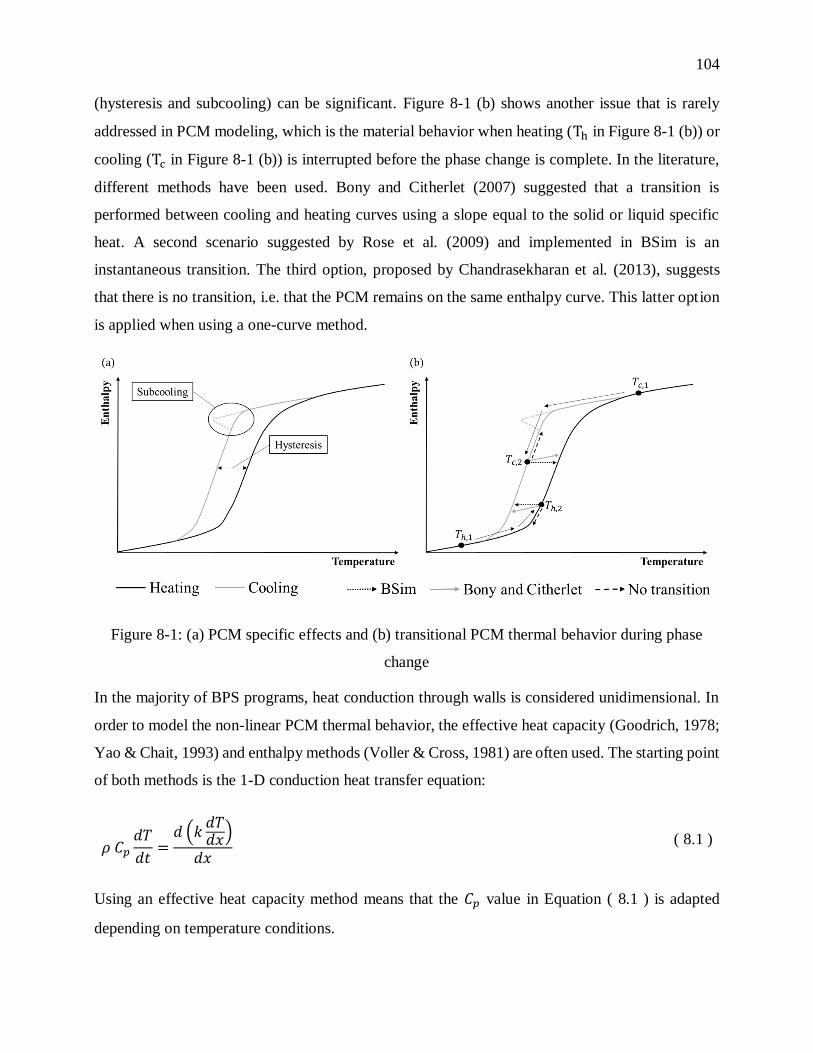
104
(hysteresis and subcooling) can be significant. Figure 8-1 (b) shows another issue that is rarely
addressed in PCM modeling, which is the material behavior when heating (Th in Figure 8-1 (b)) or
cooling (Tc in Figure 8-1 (b)) is interrupted before the phase change is complete. In the literature,
different methods have been used. Bony and Citherlet (2007) suggested that a transition is
performed between cooling and heating curves using a slope equal to the solid or liquid specific
heat. A second scenario suggested by Rose et al. (2009) and implemented in BSim is an
instantaneous transition. The third option, proposed by Chandrasekharan et al. (2013), suggests
that there is no transition, i.e. that the PCM remains on the same enthalpy curve. This latter option
is applied when using a one-curve method.
Figure 8-1: (a) PCM specific effects and (b) transitional PCM thermal behavior during phase
change
In the majority of BPS programs, heat conduction through walls is considered unidimensional. In
order to model the non-linear PCM thermal behavior, the effective heat capacity (Goodrich, 1978;
Yao & Chait, 1993) and enthalpy methods (Voller & Cross, 1981) are often used. The starting point
of both methods is the 1-D conduction heat transfer equation:
𝜌 𝐶𝑝𝑑𝑇
𝑑𝑡=𝑑 (𝑘
𝑑𝑇𝑑𝑥)
𝑑𝑥
( 8.1 )
Using an effective heat capacity method means that the 𝐶𝑝 value in Equation ( 8.1 ) is adapted
depending on temperature conditions.

105
An enthalpy formulation can be expressed, knowing that the variation of enthalpy ∆𝐻 of a material
going from an initial temperature 𝑇𝑖 to a final temperature 𝑇𝑓 is given by the following equation:
∆𝐻 = ∫ 𝐶𝑝 𝑑𝑇𝑇𝑓
𝑇𝑖
( 8.2 )
Combining Equations ( 8.1 ) and ( 8.2 ), the governing conduction heat transfer equation can be
reformulated using an enthalpy term:
𝜌𝑑𝐻
𝑑𝑡=𝑑 (𝑘
𝑑𝑇𝑑𝑥)
𝑑𝑥
( 8.3 )
Table 8-1 presents different models that can be used in TRNSYS to simulate a wall with PCM.
These TRNSYS models are encapsulated in components called “Types”:
o Type 1270 (Thermal Energy Systems Specialists, 2012) is a very simple PCM model: it
considers a constant-temperature phase change and a spatially uniform temperature inside
the PCM layer. Type 1270 is only able to model a PCM layer and must be complemented
with Type 56 (TRNSYS multizone building model) to model the other wall parts.
o Type 260 (Kuznik, Virgone, & Johannes, 2010) uses a fully implicit finite-difference
method coupled with the effective heat capacity method to model PCM. Thermal
conductivity can be defined as variable, depending on the PCM state. Thermal properties
are based on the previous time-step. Hysteresis is not modeled.
o Type 399 (Arno Dentel & Stephan, 2013) also uses an effective heat capacity method but
the conduction heat transfer governing equation is solved with a Crank-Nicolson finite-
difference method. Thermal conductivity is constant, but two different 𝐶𝑝(𝑇) curves can be
defined for both heating and cooling processes to take hysteresis into account. Like Type
260, thermal properties are based on the previous time-step. Type 399 also has the
capability to model embedded tubes with fluid circulation for heating and cooling (known
as “active layers” in TRNSYS). This capability is unique among the components listed in
Table 8-1.
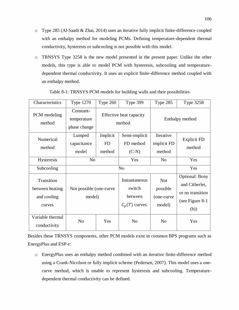
106
o Type 285 (Al-Saadi & Zhai, 2014) uses an iterative fully implicit finite-difference coupled
with an enthalpy method for modeling PCMs. Defining temperature-dependent thermal
conductivity, hysteresis or subcooling is not possible with this model.
o TRNSYS Type 3258 is the new model presented in the present paper. Unlike the other
models, this type is able to model PCM with hysteresis, subcooling and temperature-
dependent thermal conductivity. It uses an explicit finite-difference method coupled with
an enthalpy method.
Table 8-1: TRNSYS PCM models for building walls and their possibilities
Characteristics Type 1270 Type 260 Type 399 Type 285 Type 3258
PCM modeling
method
Constant-
temperature
phase change
Effective heat capacity
method Enthalpy method
Numerical
method
Lumped
capacitance
model
Implicit
FD
method
Semi-implicit
FD method
(C-N)
Iterative
implicit FD
method
Explicit FD
method
Hysteresis No Yes No Yes
Subcooling No Yes
Transition
between heating
and cooling
curves
Not possible (one-curve
model)
Instantaneous
switch
between
𝐶𝑝(𝑇) curves.
Not
possible
(one-curve
model)
Optional: Bony
and Citherlet,
or no transition
(see Figure 8-1
(b))
Variable thermal
conductivity No Yes No No Yes
Besides these TRNSYS components, other PCM models exist in common BPS programs such as
EnergyPlus and ESP-r:
o EnergyPlus uses an enthalpy method combined with an iterative finite-difference method
using a Crank-Nicolson or fully implicit scheme (Pedersen, 2007). This model uses a one-
curve method, which is unable to represent hysteresis and subcooling. Temperature-
dependent thermal conductivity can be defined.

107
o ESP-r also proposes a PCM model based on the effective heat capacity method (Heim &
Clarke, 2004) and solved with a finite-difference method. The thermal conductivity can be
defined for solid and liquid states. The original implementation cannot model hysteresis or
subcooling. Geissler (2008) recently implemented in ESP-r a development version of a
subroutine based on the work of Hoffman (2006) allowing to model hysteresis.
8.2 Objectives
This paper presents a newly developed TRNSYS component (Type) used for simulating a wall
including layer(s) with temperature-dependent properties. It also presents its numerical validation
using wall test cases proposed by the International Energy Agency and a discussion about its
performance in terms of CPU time and the number of nodes implemented in the model. Practical
examples are used to demonstrate the advantage of using an enthalpy method instead of an effective
heat capacity method. Particular attention is given to instances in which some models can miss
phase change episodes and to the PCM thermal behavior when phase change is interrupted
(transitional behavior between heating and cooling curves). This paper ends with a discussion about
subcooling modeling.
The experimental validation of the new model and the methodology to use it in conjunction with
the TRNSYS multizone building model (Type 56) are discussed in Part II of this paper (Delcroix,
Kummert, & Daoud, 2015b).
8.3 Model algorithm
The proposed model is intended to be used within whole building performance simulation. In line
with the assumptions generally made when calculating the building heat balance, heat transfer
through walls is assumed to be unidimensional. A wall model using a 1-D finite-difference method
can be represented such as in Figure 8-2. The wall is spatially discretized in nodes with heat storage
capacity. Two nodes are separated by a thermal resistance 𝑅. The length ∆𝑥 is the half-space
represented by a node or the whole space represented by a half-node. Half-nodes are the first and
last nodes of each layer.
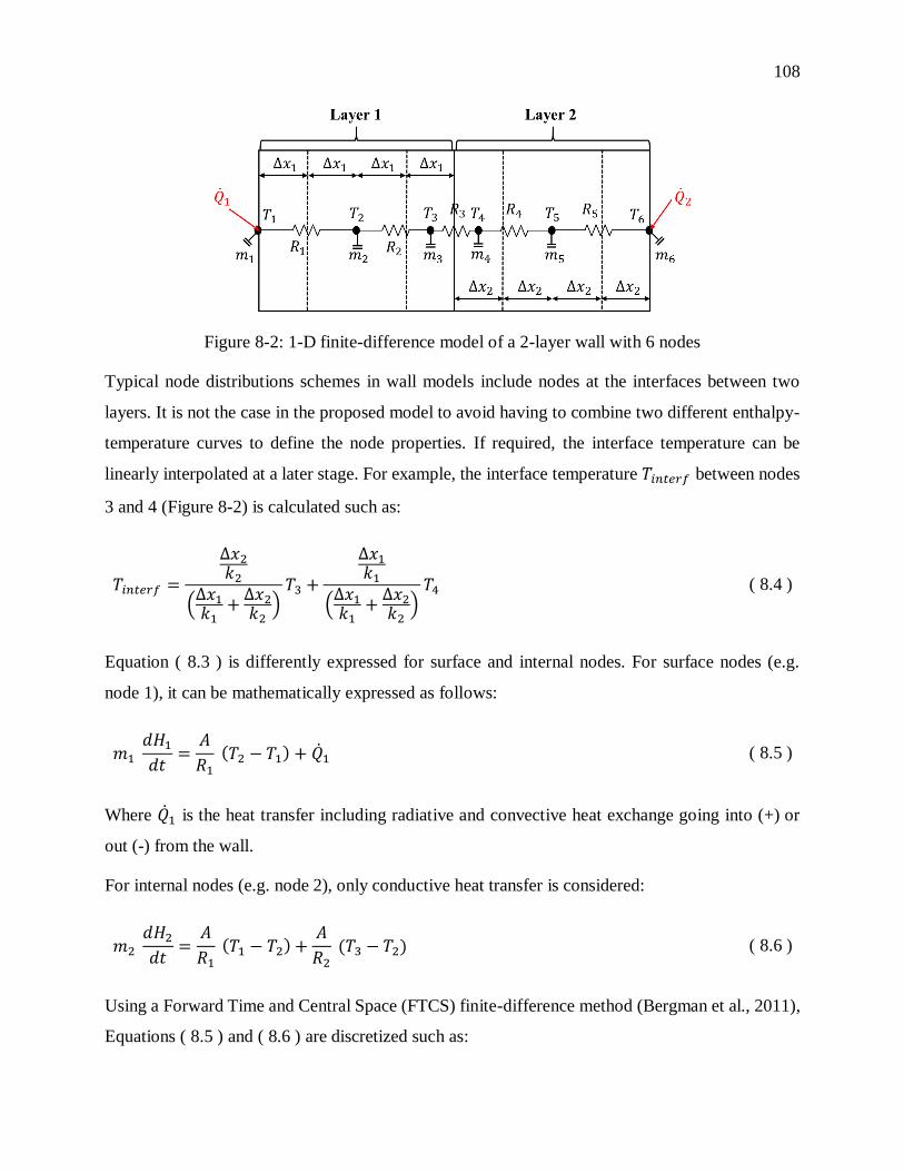
108
Figure 8-2: 1-D finite-difference model of a 2-layer wall with 6 nodes
Typical node distributions schemes in wall models include nodes at the interfaces between two
layers. It is not the case in the proposed model to avoid having to combine two different enthalpy-
temperature curves to define the node properties. If required, the interface temperature can be
linearly interpolated at a later stage. For example, the interface temperature 𝑇𝑖𝑛𝑡𝑒𝑟𝑓 between nodes
3 and 4 (Figure 8-2) is calculated such as:
𝑇𝑖𝑛𝑡𝑒𝑟𝑓 =
∆𝑥2𝑘2
(∆𝑥1𝑘1
+∆𝑥2𝑘2)𝑇3 +
∆𝑥1𝑘1
(∆𝑥1𝑘1
+∆𝑥2𝑘2)𝑇4 ( 8.4 )
Equation ( 8.3 ) is differently expressed for surface and internal nodes. For surface nodes (e.g.
node 1), it can be mathematically expressed as follows:
𝑚1 𝑑𝐻1𝑑𝑡
=𝐴
𝑅1 (𝑇2 − 𝑇1) + ��1 ( 8.5 )
Where ��1 is the heat transfer including radiative and convective heat exchange going into (+) or
out (-) from the wall.
For internal nodes (e.g. node 2), only conductive heat transfer is considered:
𝑚2 𝑑𝐻2𝑑𝑡
=𝐴
𝑅1 (𝑇1 − 𝑇2) +
𝐴
𝑅2 (𝑇3 − 𝑇2) ( 8.6 )
Using a Forward Time and Central Space (FTCS) finite-difference method (Bergman et al., 2011),
Equations ( 8.5 ) and ( 8.6 ) are discretized such as:
109
𝐻1𝑡+1 =
∆𝑡 𝐴
𝑅1 𝑚1
(𝑇2𝑡 − 𝑇1
𝑡) +∆𝑡 ��1
𝑚1+ 𝐻1
𝑡 ( 8.7 )
And:
𝐻2𝑡+1 =
∆𝑡 𝐴
𝑅1 𝑚2
(𝑇1𝑡 − 𝑇2
𝑡) +∆𝑡 𝐴
𝑅2 𝑚2
(𝑇3𝑡 − 𝑇2
𝑡) + 𝐻1𝑡 ( 8.8 )
Since the FTCS method is explicit, stability conditions (Bergman et al., 2011) must be met. For
internal nodes, the Fourier number 𝐹𝑜 must be equal to or lower than 0.5:
Fo =𝛼 ∆𝑡
∆𝑥2 ≤
1
2 ( 8.9 )
The stability condition required for the surface nodes involves the Biot number and is often more
restrictive:
Fo (1 + Bi) =𝛼 ∆𝑡
∆𝑥2(1 +
ℎ𝑔 ∆𝑥
𝑘) ≤
1
2 ( 8.10 )
The choice of the number of nodes 𝑛 per layer depends on the thermal diffusivity 𝛼, the time-step
∆𝑡, the thickness 𝐿 and the space discretization constant 𝐶 (Equation ( 8.11 )). This constant is in
fact the inverse of the Fourier number that will result from the discretization, and it is traditionally
set to a value of 3 in order to obtain a Fourier number of 1/3 which meets the stability criterion.
This method is for example used in EnergyPlus (2014).
𝑛 = 𝑓𝑙𝑜𝑜𝑟 (𝐿
√𝐶 𝛼 ∆𝑡) ( 8.11 )
The minimum number of nodes per layer is set to 3. An uneven number of nodes is also imposed
so that there is always one node for the center of the layer.
Figure 8-3 presents a diagram of the steps performed by the proposed model. A first initialization
step deals with obtaining and checking input parameters and external files. The external files define
the temperature-dependent thermal conductivity and the 𝐻(𝑇) curve(s) of each layer. This step also
sets the number of nodes (as defined by Equation ( 8.11 )) and the internal time-step required to

110
meet the stability conditions (Equations ( 8.9 ) and ( 8.10 )). The worst case scenario is used to
meet the stability conditions, i.e. using the most diffusive properties (the highest thermal
conductivity and the lowest specific heat for layers with variable properties).
The next step stores variables that will be required the next time the same instance of the Type will
be used (TRNSYS components can be used several times in the same simulation).
Once the simulation starts, two major loops are performed: one for each simulation time-step and
one for internal time-steps. For each internal time-step, the first stage consists in calculating the
new enthalpy values 𝐻𝑛𝑒𝑤 for each node, depending on initial conditions (𝐻𝑜𝑙𝑑 and 𝑇𝑜𝑙𝑑) and
boundary conditions (Equations ( 8.7 ) and ( 8.8 )). A second step consists in computing the new
node temperatures 𝑇𝑛𝑒𝑤. For a layer without variable thermal capacity, the following equation is
applied:
𝑇𝑛𝑒𝑤 = 𝑇𝑜𝑙𝑑 +𝐻𝑛𝑒𝑤 − 𝐻𝑜𝑙𝑑
𝐶𝑝 ( 8.12 )
For layers with variable thermal capacity, their new node temperatures depend on the 𝐻(𝑇) graph.
Figure 8-4 takes the most complex case: the PCM thermal behavior is defined by two curves
including subcooling. The graph is divided in five possible zones. Zones 1 and 2 are respectively
the heating and cooling curves (excluding subcooling). Zone 3 is accessible only if transition
between heating and cooling curves is allowed when phase change is interrupted (see Figure 8-1
(b)). The behavior during such an interrupted phase change is set by one of the Type’s parameters.
Zone 4 is the subcooling curve. It is accessible only if the entire PCM is initially totally liquid (𝐻 ≥
𝐻𝑙𝑖𝑞𝑢𝑖𝑑) and experiences a continuous cooling process. When subcooling occurs, it is assumed that
the entire layer experiences this effect (as explained further in section 8.8). Finally, zone 5 is a
transition phase if heating interrupts subcooling. In this case, new temperatures are computed using
a 𝐶𝑝 value equivalent to the specific heat in the liquid state.
Once all node temperatures are determined, new finite-difference coefficients must be computed if
one or more layers has a variable thermal conductivity (depending on the final temperature). If
there is no variable thermal conductivity, the finite-difference coefficients remain constant during
the whole simulation. These steps are repeated until the entire internal loop is completed.

111
The next step consists in setting output values. TRNSYS requires average values to be exchanged
between Types, so average temperatures 𝑇𝑚𝑒𝑎𝑛 are computed as follows:
𝑇𝑚𝑒𝑎𝑛 =𝑇𝑓 + 𝑇𝑖2
( 8.13 )
The variation of the enthalpy inside the wall over a time-step is also set as output and is equal to
the difference between initial and final enthalpy values 𝐻𝑖 and 𝐻𝑓 .
Figure 8-3: Process scheme of the algorithm
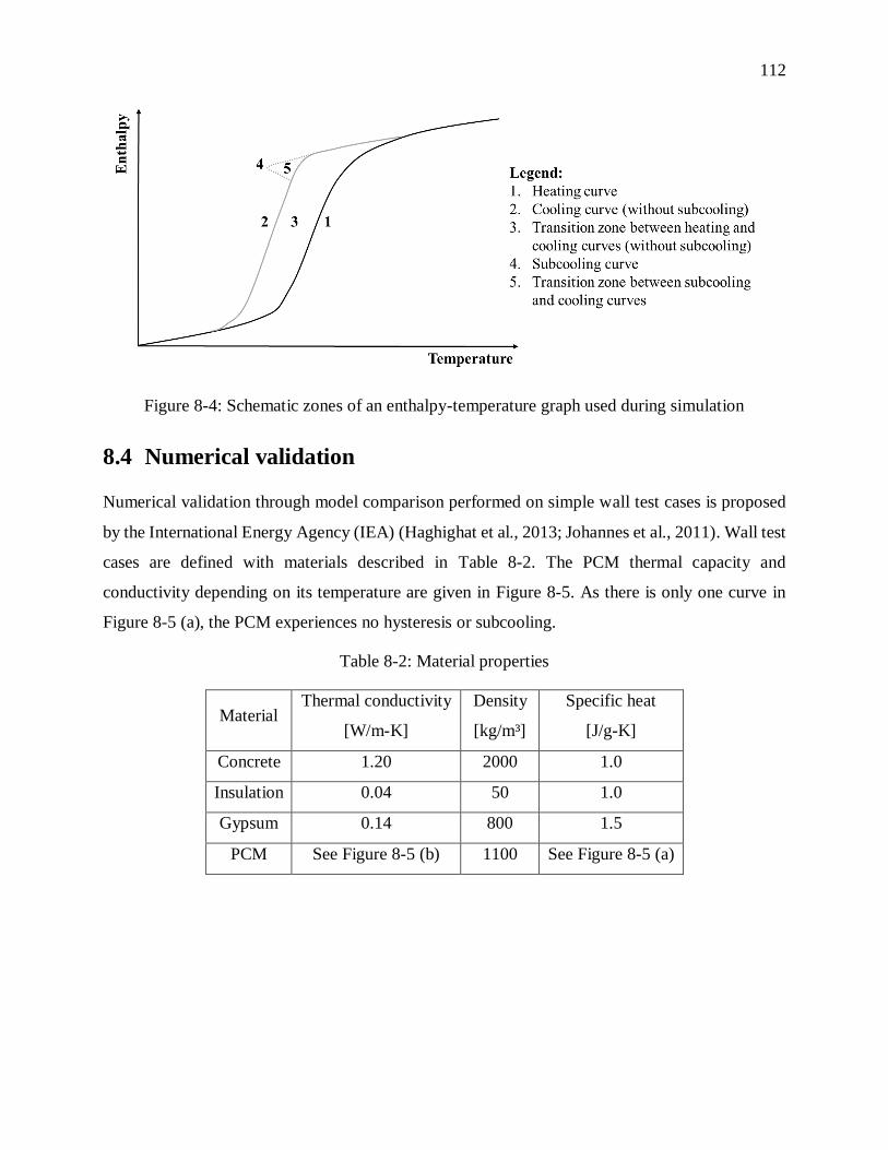
112
Figure 8-4: Schematic zones of an enthalpy-temperature graph used during simulation
8.4 Numerical validation
Numerical validation through model comparison performed on simple wall test cases is proposed
by the International Energy Agency (IEA) (Haghighat et al., 2013; Johannes et al., 2011). Wall test
cases are defined with materials described in Table 8-2. The PCM thermal capacity and
conductivity depending on its temperature are given in Figure 8-5. As there is only one curve in
Figure 8-5 (a), the PCM experiences no hysteresis or subcooling.
Table 8-2: Material properties
Material Thermal conductivity
[W/m-K]
Density
[kg/m³]
Specific heat
[J/g-K]
Concrete 1.20 2000 1.0
Insulation 0.04 50 1.0
Gypsum 0.14 800 1.5
PCM See Figure 8-5 (b) 1100 See Figure 8-5 (a)
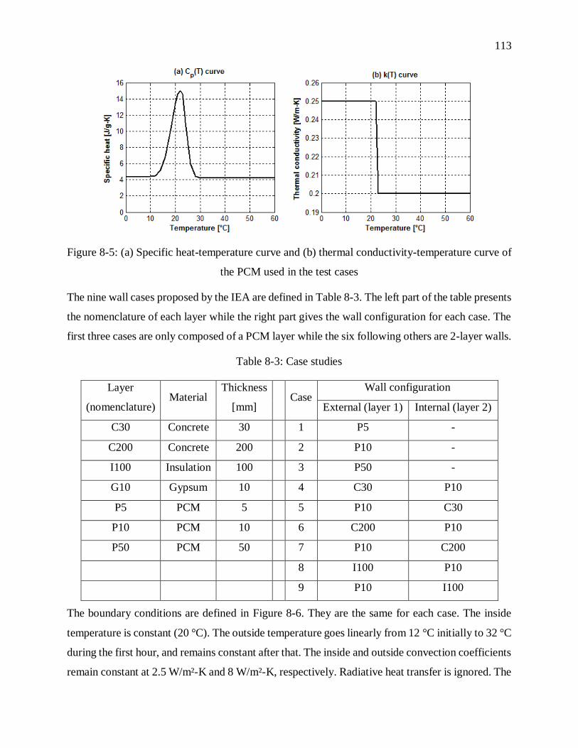
113
Figure 8-5: (a) Specific heat-temperature curve and (b) thermal conductivity-temperature curve of
the PCM used in the test cases
The nine wall cases proposed by the IEA are defined in Table 8-3. The left part of the table presents
the nomenclature of each layer while the right part gives the wall configuration for each case. The
first three cases are only composed of a PCM layer while the six following others are 2-layer walls.
Table 8-3: Case studies
Layer
(nomenclature) Material
Thickness
[mm] Case
Wall configuration
External (layer 1) Internal (layer 2)
C30 Concrete 30 1 P5 -
C200 Concrete 200 2 P10 -
I100 Insulation 100 3 P50 -
G10 Gypsum 10 4 C30 P10
P5 PCM 5 5 P10 C30
P10 PCM 10 6 C200 P10
P50 PCM 50 7 P10 C200
8 I100 P10
9 P10 I100
The boundary conditions are defined in Figure 8-6. They are the same for each case. The inside
temperature is constant (20 °C). The outside temperature goes linearly from 12 °C initially to 32 °C
during the first hour, and remains constant after that. The inside and outside convection coefficients
remain constant at 2.5 W/m²-K and 8 W/m²-K, respectively. Radiative heat transfer is ignored. The
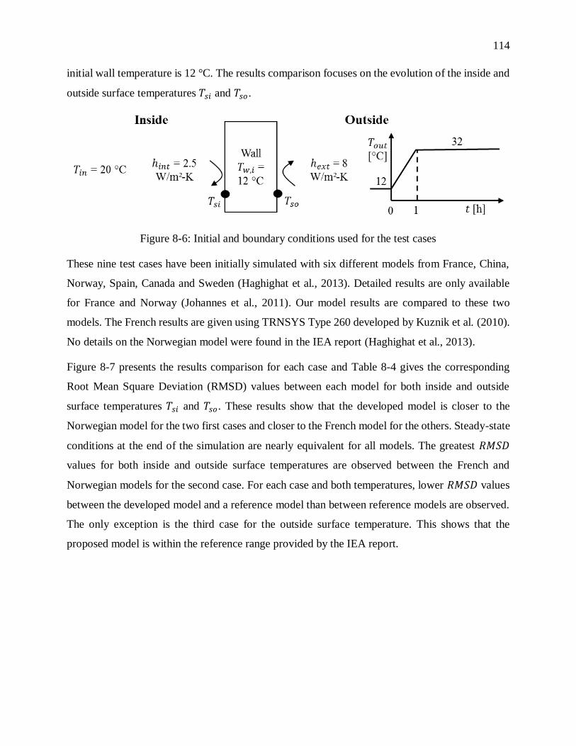
114
initial wall temperature is 12 °C. The results comparison focuses on the evolution of the inside and
outside surface temperatures 𝑇𝑠𝑖 and 𝑇𝑠𝑜.
Figure 8-6: Initial and boundary conditions used for the test cases
These nine test cases have been initially simulated with six different models from France, China,
Norway, Spain, Canada and Sweden (Haghighat et al., 2013). Detailed results are only available
for France and Norway (Johannes et al., 2011). Our model results are compared to these two
models. The French results are given using TRNSYS Type 260 developed by Kuznik et al. (2010).
No details on the Norwegian model were found in the IEA report (Haghighat et al., 2013).
Figure 8-7 presents the results comparison for each case and Table 8-4 gives the corresponding
Root Mean Square Deviation (RMSD) values between each model for both inside and outside
surface temperatures 𝑇𝑠𝑖 and 𝑇𝑠𝑜. These results show that the developed model is closer to the
Norwegian model for the two first cases and closer to the French model for the others. Steady-state
conditions at the end of the simulation are nearly equivalent for all models. The greatest 𝑅𝑀𝑆𝐷
values for both inside and outside surface temperatures are observed between the French and
Norwegian models for the second case. For each case and both temperatures, lower 𝑅𝑀𝑆𝐷 values
between the developed model and a reference model than between reference models are observed.
The only exception is the third case for the outside surface temperature. This shows that the
proposed model is within the reference range provided by the IEA report.

115
Figure 8-7: Comparison between reference models and the new model for each case
Table 8-4: Root mean square deviations [°C] for each case
Case
𝑇𝑠𝑖 –
France VS
Norway
𝑇𝑠𝑖 –
France VS
Model
𝑇𝑠𝑖 –
Norway VS
Model
𝑇𝑠𝑜 –
France VS
Norway
𝑇𝑠𝑜 –
France VS
Model
𝑇𝑠𝑜 –
Norway VS
Model
1 0.5980 0.5781 0.0511 0.5414 0.5328 0.0468
2 0.6293 0.6071 0.1285 0.5558 0.5174 0.1132
3 0.4645 0.2991 0.4001 0.2062 0.2502 0.3449
4 0.3957 0.0500 0.4325 0.3641 0.0416 0.3892
5 0.3825 0.0574 0.4040 0.3314 0.0431 0.3610
6 0.4037 0.0512 0.4195 0.3442 0.0522 0.3366
7 0.4167 0.0468 0.4003 0.3409 0.0456 0.3200
8 0.2198 0.1362 0.2162 0.0437 0.0219 0.0285
9 0.0386 0.0345 0.0379 0.2181 0.0226 0.2280

116
Surface heat-flows are also compared between all models. The inside and outside surface heat-
flows ��𝑠𝑖 and ��𝑠𝑜 are computed as follows:
��𝑠𝑖 = ℎ𝑖𝑛𝑡(𝑇𝑖𝑛 − 𝑇𝑠𝑖) ( 8.14 )
��𝑠𝑜 = ℎ𝑒𝑥𝑡(𝑇𝑜𝑢𝑡 − 𝑇𝑠𝑜) ( 8.15 )
Table 8-5 indicates the steady-state heat-flows (i.e. at the end of the 120-hour simulations) for all
models and the maximum difference observed between the developed model and one of the
reference models (France or Norway). The maximum difference of 3 % is acceptable given the
other uncertainty sources in building simulation and is also within the range of the differences
observed between the two reference models in the IEA test cases.
Table 8-5: Steady-state surface heat-flows [W/m²] (after 120 hours)
Case ��𝑠𝑖 –
France
��𝑠𝑖 –
Norway
��𝑠𝑖 –
Model
Max. diff.
with reference
[%] (��𝑠𝑖)
��𝑠𝑜 –
France
��𝑠𝑜 –
Norway
��𝑠𝑜 –
Model
Max. diff.
with reference
[%] (��𝑠𝑜)
1 21.75 21.83 21.83 0.34 21.60 21.84 21.84 1.11
2 20.75 20.88 20.88 0.60 20.80 20.88 20.88 0.38
3 15.75 15.50 15.48 1.75 16.00 15.44 15.52 3.00
4 20.00 20.00 20.00 0.00 20.00 20.00 20.00 0.00
5 20.00 20.00 20.00 0.00 20.00 20.00 20.00 0.00
6 16.25 16.13 16.15 0.62 16.00 16.32 16.24 1.50
7 16.25 16.18 16.15 0.62 16.00 16.16 16.24 1.50
8 4.00 3.88 3.90 2.50 4.00 3.92 3.92 2.00
9 4.00 3.90 3.90 2.50 4.00 3.92 3.92 2.00
Table 8-6 presents normalized 𝑅𝑀𝑆𝐷 values computed on inside and outside surface heat-flows
between the developed and reference models. Normalized 𝑅𝑀𝑆𝐷 values are calculated as follows:
𝑅𝑀𝑆𝐷𝑛𝑜𝑟𝑚 =𝑅𝑀𝑆𝐷
��𝑠−𝑠× 100 ( 8.16 )
Where ��𝑠−𝑠 is the steady-state heat-flow obtained with the reference model.

117
All values presented in Table 8-6 are below 10 %, except in 2 cases (Case 8 - ��𝑠𝑖, Case 9 - ��𝑠𝑜,
with the “Norway” reference model). Again, these normalized RMSD values are smaller than or
similar to the differences observed between the two reference models (fourth and seventh columns).
Table 8-6: Normalized 𝑅𝑀𝑆𝐷 for each case [%]
Case ��𝑠𝑖 – France
VS Model
��𝑠𝑖 – Norway
VS Model
��𝑠𝑖 – France
VS Norway
��𝑠𝑜 – France
VS Model
��𝑠𝑜 – Norway
VS Model
��𝑠𝑜 – France
VS Norway
1 6.65 0.59 6.85 6.17 0.54 6.27
2 7.31 1.54 7.54 6.22 1.36 6.68
3 4.75 6.45 7.37 3.91 5.58 3.34
4 0.63 5.41 4.95 0.52 4.86 4.55
5 0.72 5.05 4.78 0.54 4.51 4.14
6 0.79 6.50 6.21 0.82 5.16 5.38
7 0.72 6.19 6.41 0.71 4.95 5.33
8 8.51 13.95 13.74 1.37 1.82 2.79
9 2.16 2.43 2.41 1.41 14.54 13.91
8.5 Model performance – speed vs. accuracy trade-off
Model performance depends on the number of nodes and the internal time-step. Higher numbers
of nodes and lower internal time-steps impact negatively on CPU time and positively on the model
accuracy. Table 8-7 presents for 2 cases the evolution of CPU time depending on the number of
nodes and the internal time-step, which are related through the stability conditions. Higher numbers
of nodes lead to lower internal time-steps. Table 8-7 indicates that the CPU time significantly rises
when the number of nodes increases and the internal time-step is reduced. Consequently an
important consideration is the impact of the number of nodes on model precision. Using a minimal
number of nodes can be used to avoid a longer computation time. It should be considered if the
model precision is not impacted significantly by this low spatial resolution.
Figure 8-8 presents a simulation results comparison for both cases when using the minimum
number of nodes and a very large number. Table 8-8 presents the corresponding 𝑅𝑀𝑆𝐷 values
between the simulations with the minimum and a very large number of nodes. Both the figure and
the table show that no significant differences are observed, except for 𝑇𝑠𝑜 in the third case where a
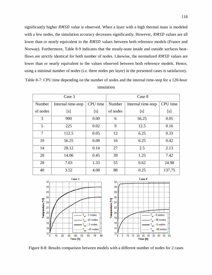
118
significantly higher 𝑅𝑀𝑆𝐷 value is observed. When a layer with a high thermal mass is modeled
with a few nodes, the simulation accuracy decreases significantly. However, 𝑅𝑀𝑆𝐷 values are all
lower than or nearly equivalent to the 𝑅𝑀𝑆𝐷 values between both reference models (France and
Norway). Furthermore, Table 8-9 indicates that the steady-state inside and outside surfaces heat-
flows are strictly identical for both number of nodes. Likewise, the normalized 𝑅𝑀𝑆𝐷 values are
lower than or nearly equivalent to the values observed between both reference models. Hence,
using a minimal number of nodes (i.e. three nodes per layer) in the presented cases is satisfactory.
Table 8-7: CPU time depending on the number of nodes and the internal time-step for a 120-hour
simulation
Case 3 Case 8
Number
of nodes
Internal time-step
[s]
CPU time
[s]
Number
of nodes
Internal time-step
[s]
CPU time
[s]
3 900 0.00 6 56.25 0.05
5 225 0.02 9 12.5 0.16
7 112.5 0.05 12 6.25 0.33
10 56.25 0.08 16 6.25 0.42
14 28.12 0.14 27 2.5 2.13
20 14.06 0.45 39 1.25 7.42
28 7.03 1.33 55 0.62 24.98
40 3.52 4.08 88 0.25 137.75
Figure 8-8: Results comparison between models with a different number of nodes for 2 cases

119
Table 8-8: 𝑅𝑀𝑆𝐷 values for a variation of the number of nodes for cases 3 and 8
Case Minimum number of nodes Large number of nodes 𝑅𝑀𝑆𝐷 for 𝑇𝑠𝑖 𝑅𝑀𝑆𝐷 for 𝑇𝑠𝑜
3 3 40 0.0588 °C 0.2704 °C
8 6 88 0.0045 °C 0.0119 °C
Table 8-9: Surface heat-flows differences for cases 3 and 8
Case 3 Case 8
Minimum number of nodes 3 6
Large number of nodes 40 88
Steady-state heat-flow ��𝑠𝑖 (minimum number of nodes) 15.48 W/m² 3.90 W/m²
Steady-state heat-flow ��𝑠𝑖 (large number of nodes) 15.48 W/m² 3.90 W/m²
Steady-state heat-flow ��𝑠𝑜 (minimum number of nodes) 15.52 W/m² 3.92 W/m²
Steady-state heat-flow ��𝑠𝑜 (large number of nodes) 15.52 W/m² 3.92 W/m²
𝑅𝑀𝑆𝐷𝑛𝑜𝑟𝑚 for ��𝑠𝑖 0.95 % 0.29 %
𝑅𝑀𝑆𝐷𝑛𝑜𝑟𝑚 for ��𝑠𝑜 13.94 % 2.43 %
8.6 Phase change detection issue
A usual problem of the effective heat capacity method used to model PCM thermal behavior is the
likelihood for phase change events to be undetected if too large time-steps are used. This method
is implemented in TRNSYS Type 399 and Type 260, which use a semi-implicit or implicit finite-
difference method where it is assumed that initial and final state properties (thermal capacity) are
similar. As illustrated in Figure 8-9, these models can then miss a phase change event since no
iterative correction is implemented. For example, the calculation in Type 399 of the future
temperature 𝑇𝑡0+1 depends on the initial and future temperature 𝑇𝑡0 and 𝑇𝑡𝑜+1 and the initial
specific heat 𝐶𝑝,𝑡0. As the new computed temperature 𝑇𝑡0+1 is beyond the phase change, the new
specific heat 𝐶𝑝,𝑡0+1 is located in the liquid state. In this case, the phase change has not been
detected.
On the other hand, the model proposed in this paper is based on the enthalpy method (Equations
( 8.5 ) and ( 8.6 )) and uses an explicit finite-difference method. The applied enthalpy method has
the benefit to remove from the equations the PCM thermal capacity property, which is highly

120
variable. Only the thermal conductivity can be variable in Equations ( 8.5 ) and ( 8.6 ), but its
dependency on temperature is weaker for typical building materials (including PCM), and it is
often assumed to be constant. The automatic adjustment of the internal time-step to meet stability
conditions for the explicit finite-difference method also ensures relatively short time-step for which
it is unlikely to “miss” phase-change events.
Figure 8-9: Phase change detection issue
In order to illustrate this phase change detection issue, the following example is proposed. A simple
1-layer wall composed of PCMs described in Table 8-10 is modeled. Initial and boundary
conditions are described in Figure 8-10. The initial wall temperature is just below the phase change
temperature range and strong heating is performed between the 23rd and 24th hours, leading to a
fast phase change event.
Table 8-10: PCM properties for the phase change detection issue case
Thickness
[m]
Density
[kg/m³]
Thermal
conductivity
[W/m-K]
Specific
heat (solid)
[J/g-K]
Specific
heat (liquid)
[J/g-K]
Latent
heat
[J/g]
Phase change
temperature range
[°C]
0.005 1000 0.5 2 2 100 20 – 21
Figure 8-10: Initial and boundary conditions used for the phase change detection issue case

121
The scenario presented in Table 8-10 and Figure 8-10 is simulated in TRNSYS using Type 399
(effective heat capacity method) and Type 3258 (enthalpy method) with a 1-hour simulation time-
step. A results comparison of both methods is presented in Figure 8-11. We can notice that results
obtained with Type 399 are affected by the user-defined internal time-step. If the internal time-step
is set to 1 hour (equivalent to the simulation time-step), the effective heat capacity model is unable
to capture the phase change event. If the internal time-step is lowered to 6 minutes, just a part of
the phase change is captured. The internal time-step must be reduced to 1 minute to model this
event accurately. At the present stage this problem remains undetected by Type 399 and the
simulation continues.
On the other hand, the enthalpy method implemented in Type 3258 is not affected by this issue.
Moreover, the internal time-step is calculated directly in the model, based on the stability
conditions.
Figure 8-11: Results comparison between TRNSYS Type 399 and Type 3258 for the phase
change detection issue case
8.7 Transitional behavior issues
In previous work (Delcroix, Kummert, & Daoud, 2015c), a bio-based PCM was implemented in a
wall and tested experimentally to assess its behavior during a phase change interruption. The
experiments consisted in placing a PCM-equipped wall successively in a warm and cold rooms.

122
It was shown that the PCM experienced a complete or partial switch from the heating to the cooling
𝐻(𝑇) curves, and conversely. This fact is in agreement with the suggestion of Bony and Citherlet
(2007) illustrated in Figure 8-1 (b). This possibility is implemented in Type 3258, in addition with
the one modeling no transition.
The effective heat capacity method implemented in Type 399 assumes an instantaneous switch
between heating and cooling 𝐶𝑝(𝑇) curves. If the PCM is heated up / cooled down, the 𝐶𝑝 value is
respectively chosen on the heating / cooling curve. Unfortunately this procedure can lead to the
energy not being conserved. Figure 8-12 illustrates a case where the solidification of a PCM is
interrupted. The PCM is initially liquid at a temperature 𝑇1. It is then cooled down (step 1) at a
temperature 𝑇2, following the cooling 𝐶𝑝(𝑇) or 𝐻(𝑇) curve. Before the end of the solidification,
the PCM is heated up (step 2) at a temperature 𝑇3. In the effective capacity method implemented
in Type 399, the 𝐶𝑝 value used is the one defined by the heating 𝐶𝑝(𝑇) curve. This is equivalent to
assuming that the whole PCM is totally solid at the beginning of the heating process (𝑇2′ instead
of 𝑇2 in Figure 8-12). In reality, the PCM should be considered in a mushy state (𝑇2). These
assumptions lead to an overestimation of the latent heat gained from 𝑇2 to 𝑇3 equivalent to the
interval illustrated by the double-arrow.
Type 399 was used to simulate a case of an interrupted solidification, as previously presented by
Delcroix et al. (2015). Figure 8-13 presents the experimental and simulated results and shows that
the effective capacity method implemented in Type 399 overestimates the PCM latent heat, as
initially illustrated in Figure 8-12.

123
Figure 8-12: Illustration of the problem caused by an instantaneous switch between cooling and
heating 𝐶𝑝(𝑇) curves
Figure 8-13: Practical consequence caused by an instantaneous switch between cooling and
heating 𝐻(𝑇) curves

124
8.8 Subcooling issue
Subcooling occurs when a liquid is cooled down below its assumed solidification temperature. It
is followed by a steep temperature increase caused by an abrupt nucleation process leading to
solidification. This results in a paradox: an enthalpy decrease leads to a temperature rise. This
anomaly causes a modeling difficulty, illustrated in Figure 8-14 with a 2-node example. A problem
arises as soon as node 𝑛1 nucleates and its temperature is higher than the other node 𝑛2 (Figure
8-14 (b)). At that moment, heat transfer takes place from 𝑛1 to 𝑛2 and the modeled temperature of
𝑛2 rises, leading to an enthalpy increase and to a higher distance to the nucleation zone. In a real
PCM, nucleation normally expands to other nodes. The model is therefore modified to take this
into account. The method adopted (Figure 8-14 (c)) consists in equalizing the temperature of 𝑛1
and 𝑛2 while keeping the enthalpy of 𝑛2 constant (𝐻2). This solution is applied only if temperature
𝑇1 is higher than 𝑇2. Once node 𝑛1 reaches the cooling curve without subcooling, this workaround
is no more applied and the temperature for all nodes is computed based on the cooling curve without
subcooling.
Figure 8-14: Subcooling modeling issue
Some PCMs (in particular most salt hydrates) exhibit a high degree of subcooling which can have
an impact in whole building simulations.
An example with a 3-layer wall is discussed hereafter to illustrate the impact of subcooling
modeling. The layers properties are given in Table 8-11. The PCM thermal conductivity 𝑘(𝑇) curve
shown in Figure 8-5 (b) is assumed, and the 𝐻(𝑇) curve given in Figure 8-5 (a) is assumed for
heating processes. Three cooling curves are added including a hysteresis and varying degrees of
subcooling (Figure 8-15), i.e. one without subcooling and the two others with low and high

125
subcooling. The overall enthalpy change between solid and liquid states is assumed to be the same
for all curves, with and without subcooling.
Table 8-11: Layers properties for the subcooling issue case (from outside to inside)
Layer Material Thermal conductivity
[W/m-K]
Density
[kg/m³]
Specific heat
[J/g-K]
Thickness
[m]
I100 Insulation 0.04 50 1.0 0.1
P10 PCM See Figure 8-5 (b) 1100 See Figure 8-15 0.01
G10 Gypsum 0.14 800 1.5 0.01
Figure 8-15: Enthalpy-temperature curves for the subcooling issue case
Initial and boundary conditions are presented in Figure 8-16. The initial wall temperature 𝑇𝑤,𝑖 is
40 °C and the wall is submitted to constant boundary conditions on both sides with a temperature
of 0 °C and a convection coefficient of 5 W/m²-K. Temperature results are presented for the PCM
layer center 𝑇𝑝𝑐𝑚 and for the inside and outside surfaces 𝑇𝑠𝑖 and 𝑇𝑠𝑜.
Figure 8-16: Initial and boundary conditions used for the subcooling issue case
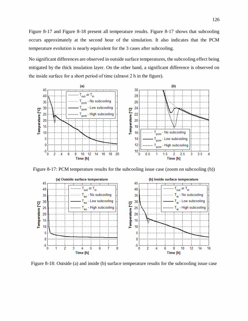
126
Figure 8-17 and Figure 8-18 present all temperature results. Figure 8-17 shows that subcooling
occurs approximately at the second hour of the simulation. It also indicates that the PCM
temperature evolution is nearly equivalent for the 3 cases after subcooling.
No significant differences are observed in outside surface temperatures, the subcooling effect being
mitigated by the thick insulation layer. On the other hand, a significant difference is observed on
the inside surface for a short period of time (almost 2 h in the figure).
Figure 8-17: PCM temperature results for the subcooling issue case (zoom on subcooling (b))
Figure 8-18: Outside (a) and inside (b) surface temperature results for the subcooling issue case

127
8.9 Conclusion
This paper presents a new model implemented in TRNSYS and named Type 3258, which is
dedicated to simulate walls including layer(s) with temperature-dependent properties. This model
uses a Forward Time and Central Space finite-difference method, combined with an enthalpy
method to represent the PCM thermal behavior. Type 3258 has been compared to other reference
models from France and Norway using wall test cases proposed by the International Energy
Agency (Annex 23). The comparison has shown that the developed model is in good agreement
with both reference models, showing differences that are smaller than or similar to the differences
existing between the two reference models. Our work also shows that the model, which uses an
enthalpy method, offers significant advantages over an effective capacity method to capture fast
transient phase change events and to model transitional PCM thermal behavior when phase change
is interrupted. The method implemented to model subcooling is also demonstrated.
The experimental validation of the new model and the methodology to use it in conjunction with
the TRNSYS multizone building model (Type 56) are discussed in Part II of this paper (Delcroix,
Kummert, & Daoud, 2015b).
Acknowledgements
The research work presented in this paper is financially supported by Hydro-Québec, FRQNT
(Fonds de Recherche du Québec en Nature et Technologies) and NSERC (Natural Sciences and
Engineering Research Council of Canada). We also would like to thank Marion Hiller, of
TRANSSOLAR, for providing TRNSYS Type 399.
References
Al-Saadi, S. N., & Zhai, Z. J. (2014). TRNSYS Type 285 - Phase Change Materials Embedded in
Wall System. Boulder, CO.
Bergman, T. L., Lavine, A. S., Incropera, F. P., & Dewitt, D. P. (2011). Fundamentals of heat and
mass transfer. Wiley.

128
Bony, J., & Citherlet, S. (2007). Numerical model and experimental validation of heat storage
with phase change materials. Energy and Buildings, 39, 1065–1072. Retrieved from
http://www.sciencedirect.com/science/article/pii/S037877880600291X
Chandrasekharan, R., Lee, E. S., Fisher, D. E., & Deokar, P. S. (2013). An Enhanced Simulation
Model for Building Envelopes with Phase Change Materials. ASHRAE Transactions,
119(2).
Crawley, D. B., Lawrie, L. K., Winkelmann, F. C., Buhl, W. F., Huang, Y. J., Pedersen, C. O.,
Strand, R. K., Liesen, R. J., Fischer, D. E., Witte, M. J., Glazer, J. (2001). EnergyPlus:
creating a new-generation building energy simulation program. Energy and Buildings, 33(4),
319–331. doi:http://dx.doi.org/10.1016/S0378-7788(00)00114-6
Danish Building Energy Institute. (2013). BSim - Building Simulation. Retrieved February 24,
2015, from http://sbi.dk/en/bsim
Delcroix, B., Kummert, M., & Daoud, A. (2015a). Modeling of a wall with phase change
materials. Part II: Experimental validation. Journal of Building Performance Simulation.
Delcroix, B., Kummert, M., & Daoud, A. (2015b). Thermal behavior mapping of a phase change
material between the heating and cooling enthalpy-temperature curves. In 6th International
Conference on Building Physics for a Sustainable Built Environment. Torino, Italy.
Dentel, A., & Stephan, W. (2013). TRNSYS TYPE 399 - Phase change materials in passive and
active wall constructions. Nürnberg.
Energy Systems Research Unit. (1998). ESP-r User Guide: The ESP-r System for Building
Energy Simulation. Glasgow.
EnergyPlus. (2014). EnergyPlus Engineering Reference.
Geissler, A. (2008). SPMCMP56 subroutine in ESP-r Source Standard Code.
129
Goodrich, L. E. (1978). Efficient numerical technique for one-dimensional thermal problems with
phase-change. International Journal of Heat and Mass Transfer, 21(5), 615.
Günther, E., Mehling, H., & Hiebler, S. (2007). Modeling of subcooling and solidification of
phase change materials. Modelling and Simulation in Materials Science and Engineering,
15, 879–892. doi:10.1088/0965-0393/15/8/005
Haghighat, F., Yu, Z., Inard, C., Michaux, G., Kuznik, F., Johannes, K., Virgone, J., Barzin, R.,
Farid, M., Bastani, A., Stathopoulos, N., El Mankibi, M., Nkwetta, D. N., Moreau, A.,
Vouillamoz, P-E., Castell, A., Adl-Zarrabi, B. (2013). Annex 23: Energy storage in
buildings of the future - Applying Energy Storage in Ultra-low Energy Buildings.
Heim, D., & Clarke, J. A. (2004). Numerical modelling and thermal simulation of PCM–gypsum
composites with ESP-r. Energy and Buildings, 36, 795–805.
doi:10.1016/j.enbuild.2004.01.004
Hoffman, S. (2006). Numerische und experimentelle Untersuchung von
Phasenübergangsmaterialien zur Reduktion hoher sommerlicher Raumtemperaturen.
Bauhaus-Universität Weimar.
Johannes, K., Virgone, J., Kuznik, F., Wang, X., Haavi, T., & Fraisse, G. (2011). Annex 23:
Applying Energy Storage in Buildings of the Future - Development of Sustainable Energy
Storage Designs for a variety of Ultra-low energy building thermal, phase change materials
and electrical storage options.
Klein, S. A., Beckman, W. A., Mitchell, J. W., Duffie, J. A., Duffie, N. A., & Freeman, T. L.
(2012). TRNSYS 17: A Transient System Simulation Program. Madison, USA: Solar
Energy Laboratory, University of Wisconsin. Retrieved from http://sel.me.wisc.edu/trnsys
Kuznik, F., & Virgone, J. (2009). Experimental investigation of wallboard containing phase
change material: Data for validation of numerical modeling. Energy and Buildings, 41(5),
561–570. doi:10.1016/j.enbuild.2008.11.022
130
Kuznik, F., Virgone, J., & Johannes, K. (2010). Development and validation of a new TRNSYS
type for the simulation of external building walls containing PCM. Energy and Buildings,
42, 1004–1009.
Pedersen, C. O. (2007). Advanced zone simulation in EnergyPlus: incorporation of variable
properties and phase change material (PCM) capability. In Building Simulation (pp. 1341–
1345). Beijing.
Rose, J., Lahme, A., Christensen, N. U., Heiselberg, P., Hansen, M., & Grau, K. (2009).
Numerical method for calculating latent heat storage in constructions containing phase
change material. In Eleventh International IBPSA Conference (pp. 400–407). Glasgow.
Thermal Energy Systems Specialists. (2012). TESSLibs3 - Type 1270: Phase Change Material
(PCM) Wall Layer for Type 56.
Voller, V. R., & Cross, M. (1981). Accurate solutions of moving boundary problems using the
enthalpy method. International Journal of Heat and Mass Transfer, 24(3), 545.
Yao, M., & Chait, A. (1993). An alternative formulation of the apparent heat capacity method for
phase change problems. Numerical Heat Transfer, Part B, Fundamentals, 24(3), 279.

131
CHAPTER 9 ARTICLE 5: MODELING OF A WALL WITH PHASE
CHANGE MATERIALS. PART II: EXPERIMENTAL VALIDATION
Delcroix, B., Kummert, M., Daoud, A., (2015). Modeling of a wall with phase change materials.
Part II: Experimental validation. Submitted to Journal of Building Performance Simulation on the
15th of July 2015.
Abstract
In Part I of this paper, a new wall model with phase change materials (PCMs) implemented in
TRNSYS is described and numerically validated. Part II focuses on its experimental validation and
on how to use this model in TRNSYS. The experimental investigation is performed in two identical
full-scale test-cells (only one with PCMs) exposed to the ambient environment. These experimental
data are primarily used to benchmark a TRNSYS simulation model of the test-cell without PCMs.
After calibration, this model is complemented with the PCM model for experimental validation.
Compared to the benchmarking procedure (without PCMs), the root mean square deviation values
between the experiments and the simulations (with PCMs) are lower or in the same order of
magnitude. The simulations reproduce the same PCM effects as observed in the experiments, such
as mitigation and time-shift effects. A discussion about computation time concludes this work.
Nomenclature
Bi Biot number [-]
𝐶𝑝 Specific heat [J/g-K]
Fo Fourier number [-]
𝐻 Enthalpy [J/kg]
ℎ Coefficient of convection [W/m²-K]
𝑘 Thermal conductivity [W/m-K]
𝑚 Mass [g]
𝑛 Number of nodes [-]
�� Heat flow [W]

132
𝑇 Temperature [°C]
𝑡 Time [s]
𝑈 Heat transfer coefficient [W/m²-K]
𝛼 Thermal diffusivity [m²/s] or coefficient of absorption [-]
∆𝑡 Time-step [s]
∆𝑥 Half-interval between 2 nodes [m]
𝜌 Density [kg/m³]
Subscripts
𝑐𝑤 Center of the wall
𝑖 i-node
𝑙 Left
𝑟 Right
𝑠𝑖 Inside surface
𝑠𝑜 Outside surface
Abbreviations
NW North-west
SW South-west
9.1 Introduction
Part I of this paper documents a new explicit finite-difference wall model with phase change
materials (PCM) implemented in TRNSYS (Delcroix, Kummert, & Daoud, 2015a). The developed
model uses an enthalpy method for modeling PCM temperature-dependent thermal capacity. A
numerical validation was successfully performed using test cases proposed by the International
Energy Agency (Haghighat et al., 2013).
The algorithm implemented in the TRNSYS multizone building model, known as Type 56, to
model transient conduction through walls is based on the Conduction Transfer Function (CTF)

133
method (TRANSSOLAR Energietechnik Gmbh, 2012). This method does not allow to model
layers with temperature-dependent properties. Using an external type in TRNSYS is then needed
to model a wall with phase change materials (PCMs). The CTF method was primarily developed
by Mitalas and Stephenson (1971) and implemented in an algorithm later by Mitalas and Arseneault
(1972). This method is based on constant CTF coefficients dedicated to model the wall thermal
response. Barbour and Hittle (2005) have proposed to adapt the CTF method to phase change
materials by generating multiple sets of CTF coefficients. During the simulation, a switching
mechanism operates in order to choose the right set of CTF coefficients corresponding to the right
properties. This method was implemented in a developer version of EnergyPlus but to the author’s
knowledge it has never been released publicly.
A more common method to model a wall including PCMs is the finite-difference method (Bergman
et al., 2011), which is used to solve the 1-D conduction heat transfer equation, formulated as
follows:
𝜌 𝐶𝑝𝑑𝑇
𝑑𝑡=𝑑 (𝑘
𝑑𝑇𝑑𝑥)
𝑑𝑥
( 9.1 )
Where:
𝐶𝑝 =𝑑𝐻
𝑑𝑇 ( 9.2 )
Combining Equations ( 9.1 ) and ( 9.2 ), the 1-D conduction heat transfer equation can be
reformulated with an enthalpy term:
𝜌𝑑𝐻
𝑑𝑡=𝑑 (𝑘
𝑑𝑇𝑑𝑥)
𝑑𝑥
( 9.3 )
Two categories of models are commonly used for simulating walls with PCM. First, the effective
heat capacity method (Goodrich, 1978; Yao & Chait, 1993) consists in solving Equation ( 9.1 )
while considering a temperature-dependent specific heat 𝐶𝑝. Second, the enthalpy method (Voller
& Cross, 1981) is based on Equation ( 9.3 ) and needs enthalpy-temperature curves to relate
temperatures to enthalpy values. Part I of the present paper describes a new model based on the

134
enthalpy method, which is named Type 3258 (Delcroix, Kummert, & Daoud, 2015a). This model
uses a Forward Time Central Space scheme to solve Equation ( 9.3 ).
Figure 9-1: 1-D finite-difference of a 1-layer wall
For the case presented in Figure 9-1, Equation ( 9.3 ) is discretized as follows:
𝐻𝑖𝑡+1 = 𝐻𝑖
𝑡 +𝑈𝑖,𝑙 𝐴 ∆𝑡
𝑚𝑖 (𝑇𝑖−1
𝑡 − 𝑇𝑖𝑡) +
𝑈𝑖,𝑟 𝐴 ∆𝑡
𝑚𝑖 (𝑇𝑖+1
𝑡 − 𝑇𝑖𝑡) ( 9.4 )
Temperature 𝑇𝑖𝑡+1 is then found from enthalpy 𝐻𝑖
𝑡+1 through user-defined enthalpy-temperature
curves. This explicit method requires to meet two different stability conditions (Bergman et al.,
2011). For internal nodes, the Fourier number Fo must be equal to or lower than 0.5:
Fo =𝛼 ∆𝑡
∆𝑥2 ≤
1
2 ( 9.5 )
For surface nodes, the stability condition is more constraining and involves the Biot number:
Fo (1 + Bi) =𝛼 ∆𝑡
∆𝑥2(1 +
ℎ ∆𝑥
𝑘) ≤
1
2 ( 9.6 )
Besides Type 3258, other models exist in TRNSYS for simulating PCM walls, such as:
o Type 1270 (Thermal Energy Systems Specialists, 2012) is a simple PCM model based on
a lumped heat balance method. It considers a constant-temperature phase change and a
spatially uniform temperature inside the PCM layer.
o Type 260 (Kuznik et al., 2010) uses a fully implicit finite-difference method coupled with
the effective heat capacity method. Thermal properties are based on the previous time-step.
It was experimentally validated by Kuznik et al. (2010).

135
o Type 399 (Arno Dentel & Stephan, 2013) uses a Crank-Nicolson finite-difference method
to solve the 1-D conduction heat equation, coupled with the effective heat capacity method
for PCM modeling. Like Type 260, thermal properties are based on the previous time-step.
It was experimentally validated by Dentel and Stephan (2010).
o Type 285 (Al-Saadi & Zhai, 2014) uses an iterative fully implicit finite-difference method
and an enthalpy method for PCM modeling. It was experimentally validated by Al-Saadi
(2014).
A PCM module also exists in other BPS programs such as EnergyPlus. The algorithm implemented
in EnergyPlus is based on an iterative semi-implicit or fully implicit finite-difference method
coupled with an enthalpy method (Pedersen, 2007). It was also numerically and experimentally
validated by Tabares-Velasco et al. (2012).
9.2 Objectives
This paper aims at validating experimentally the proposed TRNSYS model named Type 3258,
using the experimental data generated in the full-scale test-cells (equipped with PCMs or without).
An in-depth description of this test-bench and the corresponding experimental results are presented.
The experimental data of the test-cell without PCMs are primarily used to benchmark a TRNSYS
building model. This model is then complemented with the developed PCM model in order to
simulate the test-cell with PCMs. Simulations results are compared to experimental data to evaluate
if the developed model simulates adequately the PCMs effects.
This paper also discusses the coupling methods used to link the external PCM wall model (such as
Type 3258) to the TRNSYS building model (Type 56) and the resulting convergence
considerations.
9.3 Coupling between Type 56 and the external type
TRNSYS PCM models (such as the ones described in the introduction) have not been integrated
within the multizone building model (Type 56) at this time, so they must be connected to Type 56
by the TRNSYS solver. Two different methods have been proposed by TESS (Thermal Energy
Systems Specialists, 2012) and by Dentel and Stephan (2013). Both methods involve defining a
fictitious wall in Type 56 that will interact with the zone heat balance calculations (radiative and

136
convective heat transfer to and from the zone). This implies that for walls between thermal zones,
one fictitious wall is defined in each zone, and boundary conditions for these two walls are imposed
by the external wall model (see Figure 9-2 for an illustration of that principle). The coupling method
applied in the experimental validation is slightly different to both methods proposed by TESS and
by Dentel and Stephan since the surface temperatures are calculated only in Type 56. This
alternative is explained in the Appendix.
Figure 9-2: Principle of the coupling between Type 56 and the external PCM wall model
Since the external type and Type 56 are connected to each other and exchange consequently
information, convergence considerations matter. When simulating a whole system, TRNSYS
solves one component at a time and then performs iterations until convergence between all
components is reached. Convergence is verified from the input values variation, such as illustrated
in Figure 9-3. If inputs change more than the user-defined tolerance, new iterations are performed
until convergence is reached. A maximum number of iterations is defined by the user to avoid
infinite loops. If this limit is reached, TRNSYS proceeds to the next time-step with a “warning”
message indicating that a specified type did not reach convergence. If an excessive number of
warning is reached (defined by the user), the simulation stops and an error message is generated.

137
Type 56
Wall type
Other types...
TRNSYS
kernel
Do inputs
change more
than tolerance?
Proceed to
next time-step
No
Number of
iterations > limit?Yes
No
Number of
warnings > limit?
Yes
No
Stop
Yes
Figure 9-3: TRNSYS solution methodology (adapted from (Jost, 2012))
9.4 Experimental setup for PCM testing
In order to validate the new model for PCM-equipped walls, experimentations were performed in
a test-bench composed of two similar test-cells. One is equipped with PCM while the other is not.
9.4.1 PCM description
The chosen material is a bio-based PCM composed of biodegradable soybean and palm oil, mixed
with additives (gelling agent and fire retardant). It is commercially provided in pouches, as
illustrated in Figure 9-4.
Figure 9-4: PCM pouches
The main properties are presented in Table 9-1. Most properties are known for the material without
the additives (Entropy Solutions Inc., 2011). After mixing with additives (Phase change energy
solutions, 2014), only a few properties are known. The density and thermal conductivity have been
obtained through additional experimentations.

138
Table 9-1: PCM properties
Without additives With additives
Phase change temperature 23 °C Phase change temperature 23 °C
Latent heat storage capacity 203 J/g Latent heat storage
capacity 165-200 J/g
Density 830 kg/m³
Specific heat (solid) 1.84 J/g-K Weight per unit surface 1.465 kg/m²
Specific heat (liquid) 1.99 J/g-K Density 883 kg/m³ *
Thermal conductivity (solid) 0.207 W/m-K Thermal conductivity
(solid and liquid) 0.212 W/m-K **
Thermal conductivity (liquid) 0.171 W/m-K
* Experimental measurements (standard deviation: ± 15 kg/m³) – not from manufacturer
** Experimental measurements (standard deviation: ± 0.022 W/m-K) – not from manufacturer
Figure 9-5 presents the results of a Differential Scanning Calorimetry (DSC) test performed by the
manufacturer (with additives). Figure 9-5 (a) shows the variation of the heat flow depending on the
material temperature. Positive and negative values correspond respectively to heat release and
absorption. Figure 9-5 (b) gives the corresponding enthalpy-temperature curves. These graphs
shows that the fusion and solidification occur over different temperature ranges: between 20 °C
and 25 °C for fusion and between 15 °C and 20 °C for solidification. A resulting hysteresis of
around 5 °C is then observed.
Figure 9-5: (a) DSC test and (b) resulting enthalpy-temperature curves (adapted from (Phase
change energy solutions, 2008)).

139
9.4.2 PCM-equipped walls
The tested PCM-equipped wall consist of a double layer of plastic film with PCM pouches between
two plywood boards, as illustrated in Figure 9-6. Equivalent walls were also built but without PCM,
with air between both plywood boards. Both kind of walls are instrumented with thermocouples as
shown in Figure 9-6. For walls without PCM, only three thermocouples were added (center, outside
and inside surfaces). These walls are added to the inside surfaces of both test-cells (with and
without PCM) and have approximately a length of 2.4 m and a width of 0.5 m.
Figure 9-6: Instrumented PCM-equipped wall
9.4.3 Test-cells and instrumentation
The test bench is located at the energy technology laboratory (Hydro-Québec Research Institute)
in Shawinigan (QC, Canada) and consists of two identical test-cells, which are wood-frame
constructions. Newly built walls with and without PCM are fitted on the inside surfaces of the
external walls oriented north-west and south-west, as illustrated in Figure 9-7. Both test-cells are
heated with electric baseboards with a power of 1500 W. They are controlled by electronic
thermostats whose the algorithm is not known.
Figure 9-7: Test-bench description

140
Table 9-2 presents the U-values of each external surfaces, the infiltration and the dimensions of
both test-cells.
Table 9-2: U-values, infiltration and dimensions of test-cells
U-values Infiltration Dimensions
External wall 0.28 W/m²-K
0.1 h-1
Length 5.49 m
Roof 0.19 W/m²-K Width 3.66 m
Slab 0.14 W/m²-K Height 2.44 m
Door 1.25 W/m²-K Window area 1.19 m²
Window 1.6 W/m²-K Glass-door
area 3.91 m²
Glass-door 1.6 W/m²-K
Both test-cells are similarly instrumented with sensors which measure electric energy use for
heating, air dry bulb temperatures at different heights and inside surface temperatures (walls,
ceiling, floor and windows). The added walls are also instrumented, as shown in Figure 9-6. A
weather station is located next to the test-bench.
9.4.4 Tests description
Tests were carried out from the end of February to the end of July 2013. During the heating season,
different temperature set-point scenarios were tested. On the other hand, the temperature in the test-
cells during the cooling season was allowed to float. Table 9-3 presents the scenarios and their
strategies. The extreme set-back scenario was tested in order to highlight the PCM effects, i.e. the
PCM melting when the set-point is switched to 30 °C and the solidification after each set-point
temperature fall.
9.4.5 Experimental results
Figure 9-8 (a) compares the evolution of the temperatures of the indoor room air and in the center
of the added walls for the test-cell with PCM and without PCM for the residential scenario during
two days (17-03 and 18-03). During the day, solar radiation overheats the test-cells and the indoor
air temperature rises significantly. In the PCM-equipped test-cell, the PCMs allow mitigating the
temperature increase by 2 °C by storing more energy in the walls. The temperature difference at
the center of the added walls is significant, showing the impact of PCMs on the wall transient
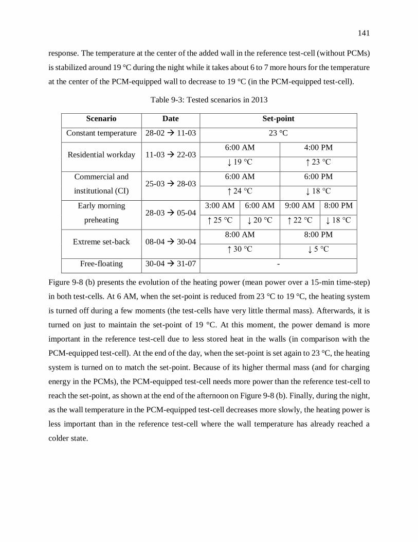
141
response. The temperature at the center of the added wall in the reference test-cell (without PCMs)
is stabilized around 19 °C during the night while it takes about 6 to 7 more hours for the temperature
at the center of the PCM-equipped wall to decrease to 19 °C (in the PCM-equipped test-cell).
Table 9-3: Tested scenarios in 2013
Scenario Date Set-point
Constant temperature 28-02 11-03 23 °C
Residential workday 11-03 22-03 6:00 AM 4:00 PM
↓ 19 °C ↑ 23 °C
Commercial and
institutional (CI) 25-03 28-03
6:00 AM 6:00 PM
↑ 24 °C ↓ 18 °C
Early morning
preheating 28-03 05-04
3:00 AM 6:00 AM 9:00 AM 8:00 PM
↑ 25 °C ↓ 20 °C ↑ 22 °C ↓ 18 °C
Extreme set-back 08-04 30-04 8:00 AM 8:00 PM
↑ 30 °C ↓ 5 °C
Free-floating 30-04 31-07 -
Figure 9-8 (b) presents the evolution of the heating power (mean power over a 15-min time-step)
in both test-cells. At 6 AM, when the set-point is reduced from 23 °C to 19 °C, the heating system
is turned off during a few moments (the test-cells have very little thermal mass). Afterwards, it is
turned on just to maintain the set-point of 19 °C. At this moment, the power demand is more
important in the reference test-cell due to less stored heat in the walls (in comparison with the
PCM-equipped test-cell). At the end of the day, when the set-point is set again to 23 °C, the heating
system is turned on to match the set-point. Because of its higher thermal mass (and for charging
energy in the PCMs), the PCM-equipped test-cell needs more power than the reference test-cell to
reach the set-point, as shown at the end of the afternoon on Figure 9-8 (b). Finally, during the night,
as the wall temperature in the PCM-equipped test-cell decreases more slowly, the heating power is
less important than in the reference test-cell where the wall temperature has already reached a
colder state.
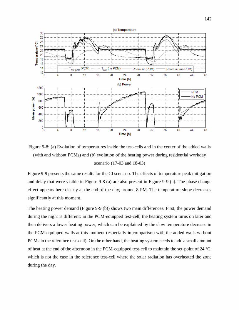
142
Figure 9-8: (a) Evolution of temperatures inside the test-cells and in the center of the added walls
(with and without PCMs) and (b) evolution of the heating power during residential workday
scenario (17-03 and 18-03)
Figure 9-9 presents the same results for the CI scenario. The effects of temperature peak mitigation
and delay that were visible in Figure 9-8 (a) are also present in Figure 9-9 (a). The phase change
effect appears here clearly at the end of the day, around 8 PM. The temperature slope decreases
significantly at this moment.
The heating power demand (Figure 9-9 (b)) shows two main differences. First, the power demand
during the night is different: in the PCM-equipped test-cell, the heating system turns on later and
then delivers a lower heating power, which can be explained by the slow temperature decrease in
the PCM-equipped walls at this moment (especially in comparison with the added walls without
PCMs in the reference test-cell). On the other hand, the heating system needs to add a small amount
of heat at the end of the afternoon in the PCM-equipped test-cell to maintain the set-point of 24 °C,
which is not the case in the reference test-cell where the solar radiation has overheated the zone
during the day.

143
Figure 9-9: (a) Evolution of temperatures inside the test-cells and in the center of the added walls
(with and without PCMs) and (b) evolution of the heating power during CI scenario (26-03 and
27-03)
The detailed temperature measurements within the walls showed two other interesting effects.
First, the temperature gradient inside a wall is strongly different, as shown in Figure 9-10. It
presents the evolution of air and walls temperatures during the extreme set-back scenario (without
(a) and with (b) PCMs). Figure 9-10 (a) shows moderate temperature gradients since all
temperatures are relatively close. PCM-equipped walls (Figure 9-10 (b)) show a different dynamic
response. The increased thermal mass makes the wall center the coldest spot (for a short time)
during a temperature rise while it becomes the warmest point (for a longer period) during a
temperature fall.

144
Figure 9-10: Evolution of the temperature gradient in the added walls without (a) and with (b)
PCM during the extreme set-back scenario (13-04 and 14-04)
A second observable effect is the appearance of an inhomogeneous temperature pattern inside the
center of the PCM-equipped wall (𝑇𝑐𝑤,𝑎𝑖𝑟 ≠ 𝑇𝑐𝑤,𝑝𝑐𝑚), caused by the heterogeneity of the central
layer composed of air, PCMs and a small amount of plastic film (Figure 9-11). During the test,
measurements at the level of the PCMs pouches and in the air spaces besides the pouches were
carried out as shown in Figure 9-6. Two measurement points were also placed at the level of the
inside surface to evaluate if the thermal heterogeneity was extended to the inside surface. A
significant difference is observed in the central layer (especially during the phase change (around
21 - 23 °C)). It seems that this thermal heterogeneity is mitigated at the level of the inside surface
as no significant difference is visible (𝑇𝑠𝑖 = 𝑇𝑠𝑖,𝑝𝑐𝑚).

145
Figure 9-11: Illustration of the temperature heterogeneity in the PCM-equipped wall (13-04 and
14-04)
During the tests, heating consumption of both test-cells was recorded for each scenario. Figure
9-12 shows that the difference between test-cells with and without PCMs is relatively small (less
than 3 %), except for the CI scenario. The combined effect of solar radiation and a higher set-point
during the day allowed storing more energy, leading to a reduced heating use during the night.
Figure 9-12: Heating consumption for different scenarios with and without PCM
9.5 Models
This section presents models developed for both test-cells without and with PCM. The model
without PCM is considered as a benchmark. The way how the PCM layer is modeled is then
146
explained. A comparison between experimental and simulated results for the test-cell with PCM
and computation times are finally discussed.
9.5.1 Reference test-cell model and benchmarking
The test-cell is modeled without PCM to fine-tune some parameters using the measured data. The
test-cell is modeled as a wood-frame construction while considering the parameters given in Table
9-2. Among the parameters to be fine-tuned are the convection coefficients and the zone
capacitance. The inside surface convection coefficients are internally computed in TRNSYS,
according to empirical relationships (TRANSSOLAR Energietechnik Gmbh, 2012). The outside
surface convection coefficients are set to the default value suggested in TRNSYS, i.e. 18 W/m²-K.
The air capacitance in the zones is set to a value of 1.2 kJ/m³-K. The extreme set-back scenario
(see Table 9-3) is chosen for the benchmarking procedure since step-changes tests are interesting
for model calibration. The electric baseboards are not explicitly modeled in TRNSYS. Instead,
Type 56’s internal heating is used. This option calculates the amount of heat that must be added
over a time-step to match the set-point. This explains the lack of oscillations in the simulated
results.
Figure 9-13 presents a comparison between experimental and simulated results and their resulting
Root Mean Square Deviation (RMSD):
(a) The heating power.
(b) The room air temperature (mid-height).
(c) The inside surface temperature of the south-west wall (mid-height).
(d) The inside surface temperature of the north-west wall (mid-height).
(e) The inside surface temperature of the ceiling.
(f) The inside surface temperature of the floor.
All graphs present clear similarities between experiments and simulations with reasonable RMSD
values. During the presented period (from the 11th of April to the 17th of April 2013), the
experimental and simulated energy consumption are respectively 59.3 kWh and 58.4 kWh, i.e. a
low error of around 1.5 %. In Figure 9-13 (f), the presence of two peaks in the experimental
temperature results is caused by direct solar radiation hitting the thermocouple during the morning

147
(the windows are oriented South-East). This calibrated model is used as a starting point for
modeling the test-cell with PCM.
Figure 9-13: Comparison between experimental and simulated results for the test-cell without
PCM during the extreme set-back scenario (from 11-04-2013 to 17-04-2013)
9.5.2 PCM modeling
As illustrated in Figure 9-6, the PCM layer is heterogeneous. In TRNSYS, conduction heat transfer
through walls is modeled in 1-D. The PCM layer is then modeled as an equivalent layer. The
properties of both layers (the plywood board and the equivalent layer with PCM) are presented in
Table 9-4.
The equivalent density is calculated as the volumetric average of all materials included in the
equivalent layer. The thermal conductivity has been computed using THERM (Lawrence Berkeley
National Laboratory, 2011). The temperature-dependent specific-heat of the equivalent layer is
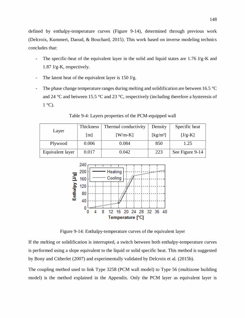
148
defined by enthalpy-temperature curves (Figure 9-14), determined through previous work
(Delcroix, Kummert, Daoud, & Bouchard, 2015). This work based on inverse modeling technics
concludes that:
- The specific-heat of the equivalent layer in the solid and liquid states are 1.76 J/g-K and
1.87 J/g-K, respectively.
- The latent heat of the equivalent layer is 150 J/g.
- The phase change temperature ranges during melting and solidification are between 16.5 °C
and 24 °C and between 15.5 °C and 23 °C, respectively (including therefore a hysteresis of
1 °C).
Table 9-4: Layers properties of the PCM-equipped wall
Layer Thickness
[m]
Thermal conductivity
[W/m-K]
Density
[kg/m³]
Specific heat
[J/g-K]
Plywood 0.006 0.084 850 1.25
Equivalent layer 0.017 0.042 223 See Figure 9-14
Figure 9-14: Enthalpy-temperature curves of the equivalent layer
If the melting or solidification is interrupted, a switch between both enthalpy-temperature curves
is performed using a slope equivalent to the liquid or solid specific heat. This method is suggested
by Bony and Citherlet (2007) and experimentally validated by Delcroix et al. (2015b).
The coupling method used to link Type 3258 (PCM wall model) to Type 56 (multizone building
model) is the method explained in the Appendix. Only the PCM layer as equivalent layer is

149
modeled in Type 3258 (with an explicit finite-difference method) while the other part of the wall
is modeled in Type 56 (with the CTF method).
9.5.3 Comparison between models and experiments
Figure 9-15 presents comparisons of different variables between experiments and simulations and
their resulting RMSD values:
(a) The heating power.
(b) The room air temperature (mid-height).
(c) The inside surface temperature of the south-west wall (mid-height).
(d) The temperature at the center of the PCM layer for the south-west wall (mid-height).
(e) The inside surface temperature of the ceiling.
(f) The inside surface temperature of the floor.
Figure 9-15: Comparison between experimental and simulated results for the test-cell with PCM
during the extreme set-back scenario (from 11-04-2013 to 17-04-2013)

150
Such as in Figure 9-13 (f), Figure 9-15 (f) presents the same peaks in the experimental temperature
results, which are caused by direct solar radiation hitting the thermocouple.
The RMSD values are generally lower than the ones measured for the test-cell without PCM.
Experimental and simulated energy consumptions are also close with respective values of 62.7
kWh and 60.4 kWh, i.e. a low error of around 3.7 %.
A results comparison between the reference and PCM-equipped test-cells shows that both
experiments and simulations indicate the same dissimilarities. Figure 9-16 presents the case of the
residential workday scenario, in which the set-point is set to 19 °C during the working hours and
to 23 °C otherwise. Experimental and simulated results show that adding PCMs mitigates
temperature extremes, as illustrated in figures (c) and (d) (in the circles). Figures (a) and (b) indicate
that the heating power presents the same dissimilarities (in the circles) between both test-cells (with
and without PCMs) in the experiments and simulations.
Figure 9-16: Results comparison between the test-cells equipped with and without PCMs during
the residential workday scenario (from 11-03-2013 to 15-03-2013)

151
However, the comparison between Figure 9-16 (c) and (d) shows that the solar radiation during the
last three days is overestimated. No shading is modeled and this can explain the overestimation of
solar radiation in the simulations.
Figure 9-17 presents the case of the commercial and institutional scenario, in which the set-point
is set to 24 °C during the working hours and to 18 °C otherwise. Such as the previous scenario, the
experimentations and simulations show that adding PCMs mitigates temperature extremes, as
illustrated in figures (c) and (d) (in the circles). Furthermore, the PCM-equipped test-cell
experiences a slower temperature decrease after a set-point drop, as similarly indicated by the
experiments and simulations. Figures (a) and (b) indicate that the heating power presents the same
dissimilarities (in the circles) between both test-cells (with and without PCMs) in the experiments
and simulations.
Figure 9-17: Results comparison between the test-cells equipped with and without PCMs during
the commercial and institutional scenario (from 25-03-2013 to 28-03-2013)
Figure 9-16 and Figure 9-17 show that the simulations reproduce the same effects than the ones
observed experimentally. Table 9-5 indicates moreover that the RMSD values between
experiments and simulations for both test-cells (with or without PCMs) are all lower than the ones

152
measured during the benchmarking procedure. It shows then that the simulations are in good
agreement with the experimentations.
Table 9-5: RMSD values between experiments and simulations for the scenarios illustrated in
Figure 9-16 and Figure 9-17
Scenario Power – RMSD Room temperature – RMSD
No PCM PCM No PCM PCM
Residential workday 145 W 139 W 1.0 °C 0.9 °C
Commercial and institutional (CI) 133 W 104 W 1.4 °C 1.1 °C
9.5.4 Computation time
Table 9-6 shows computation times for simulations of the test-cell with and without PCM and 3-D
geometry within Type 56. 3-D geometry in TRNSYS allows using a detailed calculation of
radiative heat transfer in buildings (TRANSSOLAR Energietechnik Gmbh, 2012). Computation
times are given for a 146-hour simulation using a 1-min time-step.
Table 9-6: Computation times for the test-cell simulations with the extreme set-back scenario
(146-hour simulation with a 1-min time-step)
Computation time [s] Normalized computation time
Test-cell without PCM (no 3-D) 6 s 1
Test-cell without PCM (3-D) 68 s 12
Test-cell with PCM (no 3-D) 18 s 3
As expected, simulating the test-cell without PCM and 3-D geometry requires the least computation
time. Adding 3-D geometry makes the simulation largely more time-consuming (around 12 times).
Finally, the simulation of the test-cell including PCM is around 3 times more time-consuming than
the one without 3-D and PCM. The increase in computation time seems acceptable with regard to
the new capability offered. In order to keep computation times low, it is recommended to use
Type 3258 only for including PCMs.

153
9.6 Conclusion
Conduction heat transfer through walls is currently modeled in Type 56 (multizone building model
in TRNSYS) with the CTF method. This method is unable to model layers with temperature-
dependent properties. A model based on an explicit finite-difference method was developed and
implemented in an external component, named Type 3258. This model is coupled with an enthalpy
method for PCM modeling. Part I of the current paper describes with details this model and its
numerical validation. This part presents the coupling methods to link Type 56 to the PCM wall
model and the experimental validation of Type 3258. The experimental data comes from a full-
scale test-bench composed of two identical test-cells (one equipped with PCMs and one without).
Several scenarios are tested and clear differences are observed between both test-cells. The
experimental data show that adding PCMs to building walls mitigates inside temperature variations
and produces a time shift of wall temperature extremes. Differences in heating power are small,
but temperature swings mitigation and time-shift effects are observed. A model benchmarking
procedure is firstly performed on the test-cell without PCMs, leading to a calibrated model. A
comparison between the experimental and simulated data (without PCMs) shows low RMSD
values and an error of 1.5 % for the heating consumption during the selected 7-day period. The
PCM layers are then added to this model using Type 3258 and the experimental data of the PCM-
equipped test-cell are compared to the simulated results. Compared to the benchmarking results
(without PCMs), the RMSD values between the experiments and the simulations (with PCMs) are
lower or in the same order of magnitude (for both power and temperatures data). A further result
comparison between both test-cells (with and without PCM) indicates that the simulations
reproduce adequately the impact of PCMs, i.e. mitigation and time-shift effects. Finally, the
increase in computation time caused by Type 3258 is less important than considering 3-D geometry
and seems acceptable with regard to the capability offered. However, it is recommended to use
Type 3258 only when it is needed.
Acknowledgements
The research work presented in this paper is financially supported by Hydro-Québec, FRQNT
(Fonds de Recherche du Québec en Nature et Technologies) and NSERC (Natural Sciences and

154
Engineering Research Council of Canada). We also would like to thank the energy technology
laboratory (Hydro-Québec Research Institute) where the experimentations were achieved.
Appendix - Applied coupling method between Type 56 and Type 3258
This coupling method is similar to the methods suggested by TESS and by Dentel and Stephan,
which are illustrated in Figure 9-2. The main difference consists in modeling the wall without
considering surface temperatures. The first and last nodes are modeled slightly inside the wall, as
illustrated in Figure 9-18. The surface temperatures are only calculated in Type 56 where the
boundary walls are modeled. Type 3258 is configured to model the wall without considering
surface temperatures. Such as the methods suggested by TESS and by Dentel and Stephan, the
coupling method is different for internal and external walls. As a boundary wall in Type 56 cannot
receive solar radiation, a dummy zone must be defined to model a direct contact zone between the
external and boundary walls (Figure 9-18 (b)).
The inputs from Type 56 to Type 3258 are the surface temperatures generated by Type 56. The
outputs from Type 3258 to Type 56 are the temperatures calculated for the first and last nodes by
the 1-D finite-difference model. The heat transfer coefficients between the surface temperatures
and the first and last nodes of the 1-D finite-difference model must be defined in Type 56 and are
the inverses of the thermal resistances between 𝑇𝑠𝑜,1 and 𝑇1 and between 𝑇𝑠𝑜,2 and 𝑇𝑛 (see Figure
9-18). These coefficients are given as outputs in Type 3258 and can be directly connected to Type
56. Table 9-7 presents the connections that should be performed between Type 56 and Type 3258
for this coupling method. Variable names (e.g. TSO) and output numbers (e.g. NType 18) refer to
the nomenclature used in the Type 56 manual (TRANSSOLAR Energietechnik Gmbh, 2012).
A positive side-effect of this method is the reduced constraint on the stability conditions (Equations
( 9.5 ) and ( 9.6 )). As no surface nodes are defined in the finite-difference model, the most
constraining stability condition (Equation ( 9.6 )) does not apply. A simulation speed-up is then
observed.

155
Figure 9-18: Proposed methodology to link an external wall type to Type 56
Table 9-7: Connections between Type 56 and the external wall type
Inputs from
Type 56 Notes for inputs Outputs toward Type 56
Notes for
outputs
TSO
(NType 18)
for side 1
Outside surface
temperatures
from Type 56 are
the boundary
temperatures of
the wall
Temperature at the first node (side 1) Boundary
temperatures
must be
connected to
Type 56
Temperature at the last node (side 2)
TSO
(NType 18)
for side 2
Heat transfer coefficient between the
first node and the surface temperature
(side 1) /
Heat transfer coefficient between the last
node and the surface temperature (side 2)
References
Al-Saadi, S. N. (2014). Modeling and simulation of PCM-enhanced façade systems. University
of Colorado.
Al-Saadi, S. N., & Zhai, Z. J. (2014). TRNSYS Type 285 - Phase Change Materials Embedded in
Wall System. Boulder, CO.

156
Barbour, J. P., & Hittle, D. C. (2005). Modeling Phase Change Materials With Conduction
Transfer Functions for Passive Solar Applications. Journal of Solar Energy Engineering,
128(1), 58–68. Retrieved from http://dx.doi.org/10.1115/1.2000977
Bergman, T. L., Lavine, A. S., Incropera, F. P., & Dewitt, D. P. (2011). Fundamentals of heat and
mass transfer. Wiley.
Bony, J., & Citherlet, S. (2007). Numerical model and experimental validation of heat storage
with phase change materials. Energy and Buildings, 39, 1065–1072. Retrieved from
http://www.sciencedirect.com/science/article/pii/S037877880600291X
Delcroix, B., Kummert, M., & Daoud, A. (2015a). Modeling of a wall with phase change
materials. Part I: Developement and numerical validation. Journal of Building Performance
Simulation.
Delcroix, B., Kummert, M., & Daoud, A. (2015b). Thermal behavior mapping of a phase change
material between the heating and cooling enthalpy-temperature curves. In 6th International
Conference on Building Physics for a Sustainable Built Environment. Torino, Italy.
Delcroix, B., Kummert, M., Daoud, A., & Bouchard, J. (2015). Influence of experimental
conditions on measured thermal properties used to model phase change materials. Building
Simulation: An International Journal.
Dentel, A., & Stephan, W. (2010). Thermal comfort in rooms with active PCM constructions. In
8th International Conference on System Simulation in Buildings. Liège, Belgium.
Dentel, A., & Stephan, W. (2013). TRNSYS TYPE 399 - Phase change materials in passive and
active wall constructions. Nürnberg.
Entropy Solutions Inc. (2011). PureTemp: the world’s only 100% renewable phase change
material. Retrieved July 15, 2013, from http://www.puretemp.com/
Goodrich, L. E. (1978). Efficient numerical technique for one-dimensional thermal problems with
phase-change. International Journal of Heat and Mass Transfer, 21(5), 615.

157
Haghighat, F., Yu, Z., Inard, C., Michaux, G., Kuznik, F., Johannes, K., Virgone, J., Barzin, R.,
Farid, M., Bastani, A., Stathopoulos, N., El Mankibi, M., Nkwetta, D. N., Moreau, A.,
Vouillamoz, P-E., Castell, A., Adl-Zarrabi, B. (2013). Annex 23: Energy storage in
buildings of the future - Applying Energy Storage in Ultra-low Energy Buildings.
Jost, R. (2012). Developing a run-time coupling between ESP-r and TRNSYS. École
Polytechnique de Montréal. Retrieved from
http://publications.polymtl.ca/978/1/2012_RomainJost.pdf
Kuznik, F., Virgone, J., & Johannes, K. (2010). Development and validation of a new TRNSYS
type for the simulation of external building walls containing PCM. Energy and Buildings,
42, 1004–1009.
Lawrence Berkeley National Laboratory. (2011). THERM 6.3 / WINDOW 6.3: NFRC
Simulation Manual.
Mitalas, G. P., & Arseneault, J. G. (1972). Fortran IV program to calculate z-transfer functions
for the calculation of transient heat transfer through walls and roofs. Division of Building
research, National Research Council Canada. Retrieved from http://nparc.cisti-icist.nrc-
cnrc.gc.ca/npsi/ctrl?action=shwart&index=an&req=5752842
Pedersen, C. O. (2007). Advanced zone simulation in EnergyPlus: incorporation of variable
properties and phase change material (PCM) capability. In Building Simulation (pp. 1341–
1345). Beijing.
Phase change energy solutions. (2008). BioPCM longevity cycle testing. Retrieved from
http://www.phasechange.com/index.php/en/contractor-library
Phase change energy solutions. (2014). Manufacturing innovative thermal storage technologies
for smart & sustainable buildings. Retrieved February 9, 2015, from
http://www.phasechange.com/index.php

158
Stephenson, D. G., & Mitalas, G. P. (1971). Calculation of heat conduction transfer functions for
multi-layer slabs. ASHRAE Transactions, 77(2), 117–126. Retrieved from http://nparc.cisti-
icist.nrc-cnrc.gc.ca/npsi/ctrl?action=shwart&index=an&req=5757086&lang=en
Tabares-Velasco, P. C., Christensen, C., & Bianchi, M. (2012). Verification and validation of
EnergyPlus phase change material model for opaque wall assemblies. Building and
Environment, 54, 186–196.
Thermal Energy Systems Specialists. (2012). TESSLibs3 - Type 1270: Phase Change Material
(PCM) Wall Layer for Type 56.
TRANSSOLAR Energietechnik Gmbh. (2012). TRNSYS 17 - Multizone building modeling with
Type 56 and TRNBuild. Stuttgart, Germany.
Voller, V. R., & Cross, M. (1981). Accurate solutions of moving boundary problems using the
enthalpy method. International Journal of Heat and Mass Transfer, 24(3), 545.
Yao, M., & Chait, A. (1993). An alternative formulation of the apparent heat capacity method for
phase change problems. Numerical Heat Transfer, Part B, Fundamentals, 24(3), 279.

159
CHAPTER 10 GENERAL DISCUSSION
The literature review highlights some limitations in common BPS programs such as TRNSYS,
EnergyPlus and ESP-r with respect to modeling walls that include Phase Change Materials (PCMs).
No current BPS program is capable of modeling a wall with PCMs including temperature-
dependent thermal conductivity, hysteresis and subcooling. In particular, TRNSYS is not adapted
for this purpose since conduction heat transfer through walls is modeled using the CTF method.
This method is furthermore not appropriate for short-time-step simulations (< 5 minutes) of
buildings with highly resistive and heavy walls, which is required for simulating power demand
management strategies.
The literature review also highlights the complexity of measuring PCM thermophysical properties,
and in particular the heat capacity. Measurement techniques can lead to different test results,
depending on the experimental conditions.
These challenges were addressed in the present thesis, which resulted in the contributions detailed
below.
The first main contribution is the improvement brought to the CTF method in TRNSYS multizone
building model (Type 56). As shown in Chapter 4, the proposed method to generate CTF
coefficients, based on a state-space method, can significantly reduce the gap between the
simulation time-step and the timebase value used to generate the CTF coefficients, decreasing the
stair-step effects and the corresponding inaccuracies. It is specifically useful for highly resistive
and thermally heavy walls, i.e. walls with low Fourier numbers. Unfortunately, this method cannot
ensure for all cases that the timebase value is equivalent to the simulation time-step. For extremely
difficult cases, another solution is proposed in Chapter 5. It consists of a coupling in TRNSYS
between Type 56 and another external type modeling a wall with a finite-difference method (such
as Type 3258). Using a finite-difference model for modeling walls with low Fourier number and
the CTF method for the other walls ensures that the timebase value is equivalent to the simulation
time-step. Hence Chapter 5 highlights the complementarity of both modeling methods: the finite-
difference method is appropriate for walls with low Fourier numbers while the CTF method is more
suitable for walls with higher Fourier numbers. However, modeling PCM layers requires using a
finite-difference model since the CTF method is only appropriate for walls with constant properties.

160
The second contribution of this thesis is the in-depth thermal characterization of the selected PCM
and a critical assessment of current measurement techniques for the heat capacity. Chapter 6
highlights the inability of the traditional heat capacity measurement techniques such as DSC tests
or the T-history method to obtain the effective heat capacity used for PCM modeling in building
applications. This is caused by the inadequacy between the experimental measurement conditions
(small samples and high heat transfer rates) and the actual PCM use in building applications,
especially in building envelopes (large PCM quantity and low heat transfer rates). Using an inverse
method for PCM characterization overcomes some limitations of the traditional measurement and
data processing methods, and is adaptable to different situations. An inverse method is applied on
PCM-equipped walls experimentations with varying heat transfer rates (50 cooling cases and 48
heating cases). Depending on heat transfer rates, the tested PCM behaves differently. Different heat
transfer rates (0.01 – 0.18 °C/min) impact on the phase change temperature range and on the
hysteresis between heating and cooling enthalpy-temperature curves. Results show that higher heat
transfer rates lead to higher hysteresis and colder phase change temperature ranges. Hence this
chapter highlights that a test method should be carefully chosen depending on the PCM application.
Appendices A to B detail the experiments performed to measure the density and thermal
conductivity of the tested PCM. Appendix C indicates how the thermal conductivity of the PCM
layer composed of PCM, air and plastic film is computed.
Chapter 7 focuses on the PCM thermal behavior during partial melting or solidification, i.e. when
melting or solidification is interrupted. The literature documents multiple scenarios for these cases.
Until now, no experimental validation dedicated to this specific issue was available. Chapter 7
provides an original contribution by addressing this issue experimentally. Two scenarios are tested:
first, a switch between heating and cooling enthalpy-temperature curves using a slope equivalent
to the solid or liquid specific heat; the second option consists in staying on the same curve. Two
models are developed for simulating both scenarios. A comparison between both models and the
experimentations shows a good agreement with the scenario modeling a transition between heating
and cooling curves. Hence the scenario without transition should be rejected. However, the model
with transition does not show a good agreement with the interrupted heating. In this case, the
transition between the enthalpy-temperature curves is partial. Further research should then be
conducted on the impact of different factors on the transitional behavior.
161
The final original contribution is the development and validation of a TRNSYS type dedicated to
PCM wall modeling able to simulate PCM with temperature-dependent thermal conductivity,
hysteresis and subcooling. This model is also appropriate for simulating walls with constant
properties, as illustrated in Chapter 5. Chapter 8 offers an in-depth description and a numerical
validation of the developed model named Type 3258. Type 3258 uses an explicit finite-difference
method (i.e. a Forward Time Central Space scheme) coupled with an enthalpy method for PCM
modeling. Stability conditions and a detailed description of the algorithm are presented. The
numerical validation proposed by the International Energy Agency on nine wall test cases shows
that the developed model is in good agreement with other reference models from France and
Norway. This chapter also highlights the relative superiority of the enthalpy method, compared to
the effective heat capacity. It is namely illustrated by two issues related to phase change detection
and energy conservation problems. Chapter 8 also proposes a methodology for modeling PCM
subcooling. Chapter 9 presents a further validation of Type 3258 using experimental data from test-
cells exposed to ambient environment. The experimental validation indicates that the developed
model is in agreement with experimental data and reproduces the specific effects caused by the
presence of PCMs in the test-cell. Chapter 9 also describes the possible coupling methods used to
link Type 56 to the PCM wall model (i.e. Type 3258 in our case) and discusses the corresponding
convergence considerations. An alternative method (in Chapter 9) is proposed and allows a
reduction of the model stability constraints, resulting in faster computational times. Appendix D
presents the proforma (parameters/inputs/outputs description) of Type 3258.
162
CHAPTER 11 CONCLUSION
As mentioned in the previous chapter, several contributions are presented in this thesis, i.e.:
1) Improvement of the CTF method in TRNSYS multizone building model (Type 56) based
on a state-space method. A coupling between the CTF method (Type 56) and a finite-
difference method (external type) can be performed in TRNSYS, leading to a potentially
complete resolution of the highly resistive and heavy walls problem.
2) In-depth characterization of the selected PCM, including its behavior under different
experimental conditions and during partial melting/solidification events.
3) Development and validation of a new PCM wall model, able to simulate PCM layers with
temperature-dependent thermal conductivity, hysteresis and subcooling.
Some recommendations for further research are formulated below.
The coupling between the CTF method and a finite-difference method requires a good knowledge
of the TRNSYS program to link an external type (such as Type 3258) to Type 56, which can be
seen as an unnecessarily cumbersome and error-prone process. Ideally, a finite-difference method
should be integrated directly within Type 56 for modeling heat transfer through walls.
Alternatively, a method coupling the CTF method with a finite-difference method could be worthy
to be implemented directly in Type 56 in order to benefit the complementarity of both methods.
The PCM characterization highlights the influence of the experimental conditions on the PCM
thermal behavior, in particular on the PCM hysteresis, the phase change temperature range and
during interrupted melting/solidification events. However, clear mathematical relationships
defining the impacts of experimental conditions on the PCM thermal behavior have not been
identified. This issue should be integrated in a future model. Ideally, the enthalpy-temperature
curve should be scalable, depending on the experimental conditions.
Finally, the developed and validated model uses a 1-D explicit finite-difference method for
modeling walls including PCM layers. If a highly diffusive layer (e.g. air) is included in the wall,
the explicit scheme requires very short time-steps to meet the stability conditions, leading to higher
computation times. Coupling this method with the CTF method in Type 56 is the solution proposed
in this thesis. However, a few difficulties were mentioned earlier. Ideally, an implicit method could
be implemented to avoid constraining stability conditions while considering convergence

163
considerations. The model could then select one of the two solving approaches depending on their
respective advantages.

164
REFERENCES
Alexiades, V., & Solomon, A. D. (1992). Mathematical Modeling Of Melting And Freezing
Processes. Taylor & Francis. Retrieved from
http://books.google.ca/books?id=WfJ13xBpBNYC
Al-Saadi, S. N. (2014). Modeling and simulation of PCM-enhanced façade systems. University
of Colorado.
Al-Saadi, S. N., & Zhai, Z. (John). (2013). Modeling phase change materials embedded in
building enclosure: A review. Renewable and Sustainable Energy Reviews, 21, 659–673.
doi:10.1016/j.rser.2013.01.024
Al-Saadi, S. N., & Zhai, Z. J. (2014). TRNSYS Type 285 - Phase Change Materials Embedded in
Wall System. Boulder, CO.
Alvarado, S., Marín, E., Juárez, A. G., Calderón, A., & Ivanov, R. (2012). A hot-wire method
based thermal conductivity measurement apparatus for teaching purposes. European Journal
of Physics, 33, 897–906.
Ames, W. F. (1992). Numerical methods for partial differential equations (third edit.). Boston:
Academic Press.
ASHRAE. (2013). Chapter 18 - Nonresidential Cooling and Heating Load Calculations. In
ASHRAE handbook - Fundamentals (pp. 18.15–18.20).
ASTM International. (2000). Standard Test Method for Determination of Thermal Conductivity
of Soil and Soft Rock by Thermal Needle Probe Procedure. West Conshohocken, PA, USA.
Atchonouglo, K., Banna, M., Vallée, C., & Dupré, J.-C. (2008). Inverse transient heat conduction
problems and identification of thermal parameters. Heat and Mass Transfer, 45(1), 23–29.
doi:10.1007/s00231-008-0383-7

165
Baetens, R., Jelle, B. P., & Gustavsen, A. (2010). Phase change materials for building
applications: A state-of-the-art review. Energy and Buildings, 42(9), 1361–1368.
doi:http://dx.doi.org/10.1016/j.enbuild.2010.03.026
Barbour, J. P., & Hittle, D. C. (2005). Modeling Phase Change Materials With Conduction
Transfer Functions for Passive Solar Applications. Journal of Solar Energy Engineering,
128(1), 58–68. Retrieved from http://dx.doi.org/10.1115/1.2000977
Bergman, T. L., Lavine, A. S., Incropera, F. P., & Dewitt, D. P. (2011). Fundamentals of heat and
mass transfer. Wiley.
Bony, J., & Citherlet, S. (2007). Numerical model and experimental validation of heat storage
with phase change materials. Energy and Buildings, 39, 1065–1072. Retrieved from
http://www.sciencedirect.com/science/article/pii/S037877880600291X
Braun, J. E., & Chaturvedi, N. (2002). An Inverse Gray-Box Model for Transient Building Load
Prediction. HVAC&R Research, 8(1), 73–99. Retrieved from
http://www.tandfonline.com/doi/abs/10.1080/10789669.2002.10391290
Cao, Y., & Faghri, A. (1990). A Numerical Analysis of Phase-Change Problems Including
Natural Convection. Journal of Heat Transfer, 112(3), 812–816. Retrieved from
http://dx.doi.org/10.1115/1.2910466
Carslaw, H. H., & Jaeger, J. C. (1959). Conduction of Heat in Solids (Second Edi.). Oxford
University Press.
Castell, A., Medrano, M., Castellón, C., & Cabeza, L. F. (2009). Analysis of the simulation
models for the use of PCM in buildings. In Effstock: Thermal Energy Storage for Efficiency
and Sustainability. Stockholm.
Ceylan, H. T., & Myers, G. E. (1980). Long-time solutions to heat conduction transients with
time-dependent inputs. ASME Journal of Heat Transfer, 102(1), 115–120.

166
Chandrasekharan, R., Lee, E. S., Fisher, D. E., & Deokar, P. S. (2013). An Enhanced Simulation
Model for Building Envelopes with Phase Change Materials. ASHRAE Transactions,
119(2).
Cheng, R., Pomianowski, M., Wang, X., Heiselberg, P., & Zhang, Y. (2013). A new method to
determine thermophysical properties of PCM-concrete brick. Applied Energy, 112, 988–
998. doi:10.1016/j.apenergy.2013.01.046
Cooper, J. (1998). Introduction to partial differential equation with MATLAB. Boston:
Birkhäuser.
Crank, J. (1987). Free and Moving Boundary Problems. Clarendon Press. Retrieved from
http://books.google.ca/books?id=wTB4AsVvQDsC
Crawley, D. B., Lawrie, L. K., Winkelmann, F. C., Buhl, W. F., Huang, Y. J., Pedersen, C. O.,
Strand, R. K., Liesen, R. J., Fischer, D. E., Witte, M. J., Glazer, J. (2001). EnergyPlus:
creating a new-generation building energy simulation program. Energy and Buildings, 33(4),
319–331. doi:http://dx.doi.org/10.1016/S0378-7788(00)00114-6
Danish Building Energy Institute. (2013). BSim - Building Simulation. Retrieved February 24,
2015, from http://sbi.dk/en/bsim
Delcroix, B., Kummert, M., & Daoud, A. (2015a). Modeling of a wall with phase change
materials. Part I: Developement and numerical validation. Journal of Building Performance
Simulation.
Delcroix, B., Kummert, M., & Daoud, A. (2015b). Modeling of a wall with phase change
materials. Part II: Experimental validation. Journal of Building Performance Simulation.
Delcroix, B., Kummert, M., & Daoud, A. (2015c). Thermal behavior mapping of a phase change
material between the heating and cooling enthalpy-temperature curves. In 6th International
Conference on Building Physics for a Sustainable Built Environment. Torino, Italy.

167
Delcroix, B., Kummert, M., Daoud, A., & Bouchard, J. (2014). Experimental assessment of a
phase change material in walls for heating and cooling applications. In eSim (pp. 1 – 13).
Ottawa, ON, Canada.
Delcroix, B., Kummert, M., Daoud, A., & Bouchard, J. (2015). Influence of experimental
conditions on measured thermal properties used to model phase change materials. Building
Simulation: An International Journal. doi:10.1007/s12273-015-0241-8
Delcroix, B., Kummert, M., Daoud, A., & Hiller, M. (2012). Conduction transfer functions in
TRNSYS multizone building model: current implementation, limitations and possible
improvements. In Fifth National Conference of IBPSA-USA (pp. 219 – 226). Madison,
Wisconsin.
Dentel, A., & Stephan, W. (2010). Thermal Comfort in Rooms with active PCM Constructions.
In 8th International Conference on System Simulation in Buildings (pp. 1–16). Liège,
Belgium.
Dentel, A., & Stephan, W. (2013). TRNSYS TYPE 399 - Phase change materials in passive and
active wall constructions. Nürnberg.
DuPont. (2012). Votre réponse en masse thermique aux bâtiments à faible inertie. Retrieved
October 22, 2012, from http://www.energain.fr/Energain/fr_FR/index.html
Dutil, Y., Rousse, D. R., Salah, N. Ben, Lassue, S., & Zalewski, L. (2011). A review on phase-
change materials: Mathematical modeling and simulations. Renewable and Sustainable
Energy Reviews, 15, 112–130. Retrieved from
http://www.sciencedirect.com/science/article/pii/S1364032110001589
Elsbett, G., Hiebler, S., & Mehling, H. (2006). Determination of the heat storage capacity of
PCM and PCM-objects as a function of temperature. In The Tenth International Conference
on Thermal Energy Storage. Galloway, NJ, USA.
Energy Systems Research Unit. (1998). ESP-r User Guide: The ESP-r System for Building
Energy Simulation. Glasgow.

168
EnergyPlus. (2014). EnergyPlus Engineering Reference.
Entropy Solutions Inc. (2011). PureTemp: the world’s only 100% renewable phase change
material. Retrieved July 15, 2013, from http://www.puretemp.com/
Farid, M. M., Khudhair, A. M., Razack, S. A. K., & Al-Hallaj, S. (2004). A review on phase
change energy storage: materials and applications. Energy Conversion and Management,
45(9–10), 1597–1615. doi:http://dx.doi.org/10.1016/j.enconman.2003.09.015
Fletcher, C. A. J. (1988). Computational techniques for fluid dynamics. Berlin: Springer-Verlag.
Fourier, J. (1822). Théorie analytique de la chaleur (Firmin Did.). Paris.
Geissler, A. (2008). SPMCMP56 subroutine in ESP-r Source Standard Code.
German Institute for Quality Assurance and Certification. (2009). Phase change material. Berlin,
Germany.
Giaconia, C., & Orioli, A. (2000). On the reliability of ASHRAE conduction transfer function
coefficients of walls. Applied Thermal Engineering, 20, 21–47.
Gong, Z.-X., & Mujumdar, A. S. (1997). Non-convergence versus non-conservation in effective
heat capacity methods for phase change problems. International Journal of Numerical
Methods for Heat & Fluid Flow, 7(6), 565–579.
Goodrich, L. E. (1978). Efficient numerical technique for one-dimensional thermal problems with
phase-change. International Journal of Heat and Mass Transfer, 21(5), 615.
Günther, E., Hiebler, S., Mehling, H., & Redlich, R. (2009). Enthalpy of Phase Change Materials
as a Function of Temperature: Required Accuracy and Suitable Measurement Methods.
International Journal of Thermophysics, 30(4), 1257.
Günther, E., Mehling, H., & Hiebler, S. (2007). Modeling of subcooling and solidification of
phase change materials. Modelling and Simulation in Materials Science and Engineering,
15, 879–892. doi:10.1088/0965-0393/15/8/005

169
Haghighat, F., Yu, Z., Inard, C., Michaux, G., Kuznik, F., Johannes, K., Virgone, J., Barzin, R.,
Farid, M., Bastani, A., Stathopoulos, N., El Mankibi, M., Nkwetta, D. N., Moreau, A.,
Vouillamoz, P-E., Castell, A., Adl-Zarrabi, B. (2013). Annex 23: Energy storage in
buildings of the future - Applying Energy Storage in Ultra-low Energy Buildings.
Heim, D., & Clarke, J. A. (2004). Numerical modelling and thermal simulation of PCM–gypsum
composites with ESP-r. Energy and Buildings, 36, 795–805.
doi:10.1016/j.enbuild.2004.01.004
Hittle, D. C., & Bishop, R. (1983). An improved root-finding procedure for use in calculating
transient heat flow through multilayered slabs. International Journal of Heat and Mass
Transfer, 26(11), 1685–1693.
Hoffman, S. (2006). Numerische und experimentelle Untersuchung von
Phasenübergangsmaterialien zur Reduktion hoher sommerlicher Raumtemperaturen.
Bauhaus-Universität Weimar.
Hu, H., & Argyropoulos, S. A. (1996). Mathematical modelling of solidification and melting: a
review. Modelling and Simulation in Materials Science and Engineering, 4(4), 371.
Huang, C.-H., & Jan-Yuan, Y. (1995). An inverse problem in simultaneously measuring
temperature-dependent thermal conductivity and heat capacity. International Journal of Heat
and Mass Transfer, 38(18), 3433–3441. doi:10.1016/0017-9310(95)00059-I
Hukseflux Thermal Sensors. (2014). Hukseflux Thermal Sensors MTN01. Delft, The
Netherlands. Retrieved from http://www.hukseflux.com/product/mtn01
Hydro-Québec. (2006). Réponses à la demande de renseignements no.2 de l’AQCIE/CIFQ.
Ibánez, M., Lázaro, A., Zalba, B., & Cabeza, L. F. (2005). An approach to the simulation of
PCMs in building applications using TRNSYS. Applied Thermal Engineering, 25, 1796–
1807.

170
Instructional Physics Laboratory. (2013). A Summary of Error Propagation. Cambridge, MA,
USA.
Johannes, K., Virgone, J., Kuznik, F., Wang, X., Haavi, T., & Fraisse, G. (2011). Annex 23:
Applying Energy Storage in Buildings of the Future - Development of Sustainable Energy
Storage Designs for a variety of Ultra-low energy building thermal, phase change materials
and electrical storage options.
Jost, R. (2012). Developing a run-time coupling between ESP-r and TRNSYS. École
Polytechnique de Montréal. Retrieved from
http://publications.polymtl.ca/978/1/2012_RomainJost.pdf
Klein, S. A., Beckman, W. A., Mitchell, J. W., Duffie, J. A., Duffie, N. A., & Freeman, T. L.
(2012). TRNSYS 17: A Transient System Simulation Program. Madison, USA: Solar
Energy Laboratory, University of Wisconsin. Retrieved from http://sel.me.wisc.edu/trnsys
Klimes, L., Charvat, P., & Ostry, M. (2012). Challenges in the computer modeling of phase
change materials. Materials and Technology, 46(4), 335–338.
Kosny, J., Stovall, T., Shrestha, S., & Yarbrough, D. (2010). Theoretical and Experimental
Thermal Performance Analysis of Complex Thermal Storage Membrane Containing Bio-
Based Phase-Change Material (PCM). In Building XI (p. 11).
Kravvaritis, E. D., Antonopoulos, K. A., & Tzivanidis, C. (2010). Improvements to the
measurement of the thermal properties of phase change materials. Measurement Science and
Technology, 21, 1–9.
Kula, L. W., & Yovanovich, M. M. (1991). Characteristic length of complex bodies for transient
conduction. ASME Thermal Engineering Proceedings, 1, 259–267.
Kuznik, F., & Virgone, J. (2009). Experimental investigation of wallboard containing phase
change material: Data for validation of numerical modeling. Energy and Buildings, 41(5),
561–570. doi:10.1016/j.enbuild.2008.11.022
171
Kuznik, F., Virgone, J., & Johannes, K. (2010). Development and validation of a new TRNSYS
type for the simulation of external building walls containing PCM. Energy and Buildings,
42, 1004–1009.
LAPACK. (2011). DGEEVX: computation of the eigenvalues of a general matrix. Retrieved
from http://www.netlib.org/lapack/individualroutines.html
Lawrence Berkeley National Laboratory. (2013). THERM 6.3 / WINDOW 6.3 - NFRC
Simulation Manual.
Leduc, M.-A., Daoud, A., & Le Bel, C. (2011). Developing winter residential demand response
strategies for electric space heating. In 12th Conference of International Building
Performance Simulation Association (2011) (pp. 1111–1118). Sydney.
Lemmon, E. C. (1981). Multidimensional integral phase change approximations for finite
element conduction codes. In R. W. Lewis, K. Morgan, & O. C. Zienkiewicz (Eds.),
Numerical methods in heat transfer (pp. 201–213). New-York.
Li, X. Q., Chen, Y., Spitler, J. D., & Fisher, D. (2009). Applicability of calculation methods for
conduction transfer function of building constructions. International Journal of Thermal
Sciences, 48(7), 1441–1451. doi:10.1016/j.ijthermalsci.2008.11.006
Maestre, I. R., Mena, J. D., Pérez-lombard, L., & Gallero, J. G. (2014). Fitting conduction
transfer function method to low Fourier numbers: application to ground-coupled floors.
Journal of Building Performance Simulation, 1–11. doi:10.1080/19401493.2014.974210
Marín, J. M., Zalba, B., Cabeza, L. F., & Mehling, H. (2003). Determination of enthalpy –
temperature curves of phase change materials with the temperature-history method :
improvement to temperature dependent properties. Measurement Science and Technology,
14, 184–189.
Mehling, H., & Cabeza, L. F. (2008). Heat and cold storage with PCM: An up to date
introduction into basics and applications. (D. Mewes & F. Mayinger, Eds.). Berlin: Springer.

172
Ministère des Ressources naturelles et de la Faune. (2010). Statistiques énergétiques. Retrieved
from http://www.mrn.gouv.qc.ca/energie/statistiques/statistiques-production-centrales.jsp
Mitalas, G. P. (1968). Calculation of transient heat flow through walls and roofs. ASHRAE
Transactions, 74(2), 182–188. Retrieved from http://nparc.cisti-icist.nrc-
cnrc.gc.ca/npsi/ctrl?action=shwart&index=an&req=5753857&lang=en
Mitalas, G. P., & Arseneault, J. G. (1972). Fortran IV program to calculate z-transfer functions
for the calculation of transient heat transfer through walls and roofs. Division of Building
research, National Research Council Canada. Retrieved from http://nparc.cisti-icist.nrc-
cnrc.gc.ca/npsi/ctrl?action=shwart&index=an&req=5752842
Moler, C., & Van Loan, C. (2003). Nineteen Dubious Ways to Compute the Exponential of a
Matrix, Twenty-Five Years Later. SIAM Review, 45(1), 3–49.
Morgan, K., Lewis, R. W., & Zienkiewicz, O. C. (1978). An improved algrorithm for heat
conduction problems with phase change. International Journal for Numerical Methods in
Engineering, 12(7), 1191–1195.
Morton, K. W., & Mayers, D. F. (1994). Numerical solution of partial differential equations: an
introduction. Cambridge: Cambridge University Press.
Myers, G. E. (1971). Analytical methods in conduction heat transfer (McGraw-Hil.). New-York.
Pasupathy, A., & Velraj, R. (2006). Mathematical modeling and experimental study on building
ceiling system incorporating phase change material (PCM) for energy conservation. In
ASME Conference Proceedings (pp. 59–68).
Patankar, S. (1980). Numerical heat transfer and fluid flow. CRC Press.
Pedersen, C. O. (2007). Advanced zone simulation in EnergyPlus: incorporation of variable
properties and phase change material (PCM) capability. In Building Simulation (pp. 1341–
1345). Beijing.

173
Peeters, L., & Mols, R. (2012). Zero Energy House Renovation. Retrieved February 8, 2013,
from http://www.zehr.be
Pham, Q. T. (1985). A fast, unconditionally stable finite-difference scheme for heat conduction
with phase change. International Journal of Heat and Mass Transfer, 28(11), 2079–2084.
Phase change energy solutions. (2008). BioPCM longevity cycle testing. Retrieved from
http://www.phasechange.com/index.php/en/contractor-library
Phase change energy solutions. (2014). Manufacturing innovative thermal storage technologies
for smart & sustainable buildings. Retrieved February 9, 2015, from
http://www.phasechange.com/index.php
Pipes, L. A. (1957). Matrix analysis of heat transfer problems. Journal of the Franklin Institute,
263(3), 195–206.
Poirier, D. J. (1986). On numerical methods used in mathematical modelling of phase change in
liquid metals. University of Ottawa.
Poulad, M. E., Fung, A. S., & Naylor, D. (2011). Effects of convective heat transfer coefficient
on the ability of PCM to reduce building energy demand. In 12th Conference of
International Building Performance Simulation Association (pp. 270–277). Sydney.
Recktenwald, G. W. (2011). Finite-Difference Approximations to the Heat Equation (Vol. 0).
Portland, Oregon, USA. Retrieved from http://www.f.kth.se/~jjalap/numme/FDheat.pdf
Rose, J., Lahme, A., Christensen, N. U., Heiselberg, P., Hansen, M., & Grau, K. (2009).
Numerical method for calculating latent heat storage in constructions containing phase
change material. In Eleventh International IBPSA Conference (pp. 400–407). Glasgow.
Schranzhofer, H., Puschnig, P., Heinz, A., & Streicher, W. (2006). Validation of a TRNSYS
simulation model for PCM energy storages and PCM wall construction elements. In 10th
International Conference on Thermal Energy Storage. New Jersey.

174
Seem, J. E. (1987). Modeling of heat transfer in buildings. University of Wisconsin, Madison.
Shamsundar, N., & Rooz, E. (1988). Numerical methods for moving boundary problems. In W. J.
Minkowycz, E. M. Sparrow, G. E. Schneider, & R. H. Pletcher (Eds.), Handbook of
numerical heat transfer. New-York: Wiley-Interscience.
Shamsundar, N., & Sparrow, E. M. (1975). Analysis of Multidimensional Conduction Phase
Change Via the Enthalpy Model. Journal of Heat Transfer, 97(3), 333–340. Retrieved from
http://dx.doi.org/10.1115/1.3450375
Sharma, A., Tyagi, V. V, Chen, C. R., & Buddhi, D. (2009). Review on thermal energy storage
with phase change materials and applications. Renewable and Sustainable Energy Reviews,
13(2), 318–345. doi:http://dx.doi.org/10.1016/j.rser.2007.10.005
Shrestha, S., Miller, W., Stovall, T., Desjarlais, A., Childs, K., Porter, W., Bhandary, M., Coley,
S. (2011). Modeling PCM-enhanced insulation system and benchmarking EnergyPlus
against controlled field data. In 12th Conference of International Building Performance
Simulation Association (pp. 800–807). Sydney.
Sidje, R. B. (1998). Expokit: a software package for computing matrix exponentials. ACM
Transactions on Mathematical Software, 24(1), 130–156.
Solé, A., Miró, L., Barreneche, C., Martorell, I., & Cabeza, L. F. (2013). Review of the T-history
method to determine thermophysical properties of phase change materials (PCM).
Renewable and Sustainable Energy Reviews, 26, 425–436. doi:10.1016/j.rser.2013.05.066
Spakovszki, Z. S. (2014). 19.3 Radiation heat transfer between planar surfaces. Retrieved
February 25, 2015, from
http://web.mit.edu/16.unified/www/FALL/thermodynamics/notes/node136.html
Stephenson, D. G., & Mitalas, G. P. (1971). Calculation of heat conduction transfer functions for
multi-layer slabs. ASHRAE Transactions, 77(2), 117–126. Retrieved from http://nparc.cisti-
icist.nrc-cnrc.gc.ca/npsi/ctrl?action=shwart&index=an&req=5757086&lang=en

175
Swaminathan, C. R., & Voller, V. R. (1992). A general enthalpy method for modeling
solidification processes. Metallurgical Transactions B, 23(5), 651–664.
Swaminathan, C. R., & Voller, V. R. (1993). On the enthalpy method. International Journal of
Numerical Methods for Heat & Fluid Flow, 3(3), 233–244. doi:10.1108/eb017528
Tabares-Velasco, P. C., Christensen, C., & Bianchi, M. (2012). Verification and validation of
EnergyPlus phase change material model for opaque wall assemblies. Building and
Environment, 54, 186–196.
Tabares-Velasco, P. C., Christensen, C., Bianchi, M., & Booten, C. (2012). Verification and
Validation of EnergyPlus Conduction Finite Difference and Phase Change Material Models
for Opaque Wall Assemblies. Contract, 303, 275–3000.
Tavakoli, R., & Davami, P. (2007). Unconditionally stable fully explicit finite difference solution
of solidification problems. Metallurgical and Materials Transactions B, 38(1), 121–142.
The MathWorks Inc. (2010). Matlab help. Natick, MA, USA.
The MathWorks Inc. (2014). GA - Find minimum of function using genetic algorithm. Retrieved
July 2, 2014, from http://www.mathworks.com/help/gads/ga.html
Thermal Energy Systems Specialists. (2012). TESSLibs3 - Type 1270: Phase Change Material
(PCM) Wall Layer for Type 56.
TRANSSOLAR Energietechnik Gmbh. (2012). TRNSYS 17 - Multizone building modeling with
Type 56 and TRNBuild. Stuttgart, Germany.
Voller, V. R. (1996). An overview of numerical methods for solving phase change problems. In
W. J. Minkowycz & E. M. Sparrow (Eds.), Advances in numerical heat transfer - Volume 1
(pp. 341 – 375). CRC Press.
Voller, V. R., & Cross, M. (1981). Accurate solutions of moving boundary problems using the
enthalpy method. International Journal of Heat and Mass Transfer, 24(3), 545.

176
Voller, V. R., Swaminathan, C. R., & Thomas, B. G. (1990). Fixed grid techniques for phase
change problems: a review. International Journal for Numerical Methods in Engineering,
30(4), 875–898. doi:10.1002/nme.1620300419
Waters, J. R., & Wright, A. J. (1985). Criteria for the distribution of nodes in multilayer walls in
finite-difference thermal modelling. Building and Environment, 20(3), 151–162.
Watson, E. S., O’Neill, M. J., Justin, J., & Brenner, N. (1964). A Differential Scanning
Calorimeter for Quantitative Differential Thermal Analysis. Analytical Chemistry, 36(7),
1233–1238. doi:10.1021/ac60213a019
Yao, M., & Chait, A. (1993). An alternative formulation of the apparent heat capacity method for
phase change problems. Numerical Heat Transfer, Part B, Fundamentals, 24(3), 279.
Zalba, B., Marın, J. M., Cabeza, L. F., & Mehling, H. (2003). Review on thermal energy storage
with phase change: materials, heat transfer analysis and applications. Applied Thermal
Engineering, 23(3), 251–283. doi:http://dx.doi.org/10.1016/S1359-4311(02)00192-8
Zhang, Y., Jiang, Y., & Jiang, Y. (1999). A simple method , the T -history method , of
determining the heat of fusion , specific heat and thermal conductivity of phase-change
materials. Measurement Science and Technology, 10, 201–205.

177
APPENDIX A – EXPERIMENTS ON PCM DENSITY
The PCM density is measured on ten different samples. A precision balance (resolution: 0.001
gram) and a container with a known volume and mass of 32 milliliters and 3.055 grams is used to
perform the density test measurements (Figure A-1). The PCM is in the liquid state during the
whole experimentation. Additives included in the PCM are considered in these experimentations
(contrary to the measurement performed by the manufacturer).
Figure A-1: Density test proceedings
A syringe of 10 milliliters, graduated every 0.1 mL, is used to measure the container volume. For
doing so, four draws (3 draws of 10 mL and one of 2 mL) are necessary. An uncertainty of 0.1 mL
per draw is assumed, i.e. a total uncertainty 𝛿𝑉 of 0.4 mL (for a volume V of 32 mL).
Table A-1 presents the results for each test. The average PCM mass �� is 28.261 grams and its
corresponding standard deviation 𝜎𝑚 is 0.316 grams. The uncertainty on mass measurement 𝛿𝑚 is
assumed to be the standard deviation 𝜎𝑚. The average density is given in Table A-1 and is equal
to 883.163 kg/m³. In order to obtain the uncertainty on density 𝛿𝜌, the following equation is applied
(Instructional Physics Laboratory, 2013):
𝛿𝜌 = �� √(𝛿𝑚
��)2
+ (𝛿𝑉
𝑉)2
( A.1 )
Using the actual values, Equation ( A.1 ) becomes:
𝛿𝜌 = 883.163 √(0.316
28.261)2
+ (0.4
32)2
= 14.812 𝑘𝑔/𝑚³ ( A.2 )

178
The average measured density is around 883 kg/m³ and is significantly higher than the value given
by the manufacturer (830 kg/m³ (without additives)). Considering the uncertainty, the
underestimation is between 4.4 % and 7.6 %.
Table A-1: Density measurements of 10 PCM samples
Test Mass of fulfilled container [g] PCM mass [g] Density [kg/m³]
1 31.643 28.588 893.375
2 31.469 28.414 887.938
3 31.421 28.366 886.438
4 31.315 28.260 883.125
5 30.843 27.788 868.375
6 31.060 28.005 875.156
7 31.833 28.778 899.313
8 30.993 27.938 873.063
9 31.509 28.454 889.188
10 31.076 28.021 875.656
Mean 31.316 ± 0.316 28.261 ± 0.316 883.163 ± 14.812
Density given by the manufacturer (without additives) 830
By cooling down the samples of liquid PCM, it would have been possible to evaluate the density
in solid state indicated by the volume variation. However, the solidification creates gaps
(Figure A-2) in the samples while taking the same volume. The solid density is apparently higher
than the liquid density, but it was not possible to estimate a precise value from these samples. In
short, the density given by the manufacturer is underestimated by around 6 % (if the average is
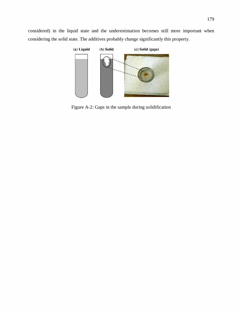
179
considered) in the liquid state and the underestimation becomes still more important when
considering the solid state. The additives probably change significantly this property.
Figure A-2: Gaps in the sample during solidification

180
APPENDIX B – EXPERIMENTS ON PCM THERMAL CONDUCTIVITY
The hot-wire method was used to evaluate experimentally the thermal conductivity of the PCM in
liquid and solid states. The principle of the hot-wire method is to heat the sample locally in its
center and to measure over the time the temperature rise at the heat injection point. Lower
temperature rises lead to higher thermal conductivities. The hot-wire method is well documented,
e.g. in (Alvarado et al., 2012; ASTM International, 2000). The volume of the PCM sample is
around 5 liters and a cylindrical container was used. Additives included in the PCM are considered
in these experimentations (contrary to the measurement performed by the manufacturer). The
needle from the hot-wire equipment was immersed in the center of the sample, as illustrated in
Figure B-1. The needle is a constant linear heating source and the heat flow is assumed to be radial.
A temperature sensor is integrated within the needle to record the evolution of temperature over
time.
Figure B-1: Hot-wire equipment scheme
The experimentations were performed in liquid (3 times) and solid (4 times) states using Hukseflux
MTN01 (Hukseflux Thermal Sensors, 2014). Figure B-2 summarizes the results of the
experimental measurements in grey compared to the values provided by the manufacturer in black
(without additives). Values from 0.184 W/m-K to 0.255 W/m-K were measured during
experimentations with an average of 0.212 W/m-K and a standard deviation of 0.022 W/m-K.
Experimental results in liquid state are very stable around 0.209 W/m-K (with a standard deviation
of 0.001 W/m-K) while the values for solid state are more variable, which is probably due to the
perturbation caused by the solidification process creating air gaps in the PCM sample. The average
value for the solid state is 0.214 W/m-K with a standard deviation of 0.030 W/m-K. The

181
measurement accuracy for the hot wire method is estimated at ± (6 % + 0.04 W/m-K), as illustrated
by the error bars in Figure B-2.
Figure B-2: Comparison between the manufacturer values and the experimental values of thermal
conductivity in liquid (L) and solid (S) states
In summary, the thermal conductivity in liquid obtained experimentally (0.209 W/m-K) is
significantly different from the value given by the manufacturer without the additives
(0.171 W/m-K), i.e. an underestimation of around 18 %. On the other hand, the measurements for
the solid state show a significant variability. The average value for the solid state (0.214 W/m-K)
is slightly higher than the liquid, which is consistent with manufacturer data. As both average
values are very close given the uncertainty, the global experimental average (0.212 W/m-K) is
deemed to be a representative value for both states.

182
APPENDIX C – EQUIVALENT LAYER THERMAL CONDUCTIVITY
As most building energy performance simulation programs only model 1-D heat conduction
through walls, each layer should be homogeneous. The PCM-equipped wall illustrated in Figure
C-1 has a central heterogeneous layer. The thermal conductivity of this layer can be obtained using
a computational tool such as THERM (Lawrence Berkeley National Laboratory, 2013). Figure C-
1 focuses on the thicknesses of each material. PCM pouches occupy 35 % of the surface. The
remainder is occupied by air voids.
Figure C-1: Scheme of the PCM-equipped wall
Table C-1 presents the thickness and thermal conductivity of each material in the PCM-equipped
wall.
Table C-1: Thickness and thermal conductivity of each material in the PCM-equipped wall
Air PCM Plastic film Plywood
Thickness 𝐿 [m] 0.003 0.008 0.005 0.001 0.006
Thermal conductivity 𝑘
[W/m-K] 0.040 0.063 0.212 0.150 0.084
The equivalent air thermal conductivity is calculated by assuming negligible convection (thin
layers), a “pure” thermal conductivity of 0.0256 W/m-K, and calculating the radiative heat transfer
with Kirchoff’s law (Bergman et al., 2011). The radiation heat transfer between planar surfaces
(Spakovszki, 2014) is given by the following equation:

183
��1 𝑡𝑜 2 =𝜎(𝑇1
4 − 𝑇24)
1휀1+1휀2− 1
( C.1 )
Where ��1 𝑡𝑜 2 is the net radiation heat transfer between surfaces 1 and 2; 𝜎 is the Stefan-Boltzmann
constant (5.67 × 10⁻⁸ W/m²-K4); 𝑇1 and 𝑇2 are the surface temperatures; 휀1 and 휀2 are the surface
emissivity’s.
Assuming a temperature difference of 1 K between 𝑇1 (294 K or 21 °C) and 𝑇2 (293 K or 20 °C)
and surface emissivity’s of 0.9, the resulting net radiation heat transfer from surface 1 to 2 is around
4.7 W/m². Considering a temperature difference of 1 K, the corresponding radiation heat transfer
coefficient is 4.7 W/m²-K.
From these assumptions, the air thermal conductivity including radiative and conductive heat
transfer can be computed as follows:
𝑘𝑎𝑖𝑟 = (0.0256
𝐿+ 4.7) × 𝐿 ( C.2 )
Equation ( C.2 ) gives air thermal conductivity values of 0.040 W/m-K (𝐿 = 0.003 m) and
0.063 W/m-K (𝐿 = 0.008 m).
The heat transfer coefficient of the configuration presented in Figure C-1 and Table C-1 has been
computed using THERM. A U-value of 1.818 W/m²-K (R = 0.550 m²K/W) is obtained for the
whole PCM-equipped wall. Removing the thermal resistance of both plywood boards (2 × 0.071
m²K/W), the thermal resistance of the equivalent layer is 0.408 m²K/W. Considering a thickness
of 17 millimeters, the equivalent layer has a thermal conductivity of 0.042 W/m-K.

184
APPENDIX D – PROFORMA OF TRNSYS TYPE 3258
This appendix describes the external files used in Type 3258 to define temperature-dependent
thermal conductivities and capacities. It also presents a list of the parameters, inputs and outputs
implemented in Type 3258 and a brief description for each element.
External files
- Data file defining temperature-dependent thermal conductivities
The first line of this file gives the number of rows and columns defined in the file. The first column
gives the temperature values in °C in ascending order. Each following column gives the
temperature-dependant thermal conductivities in W/m-K for each layer with variable thermal
conductivity. The number of rows is the same for all layers. The order of definition follows the
order of appearance from side 1 to side 2. If a layer does not have temperature-dependent thermal
conductivity, there is no need to define a column in the data file and the value given in the
parameters is used. For example, a 3-layer wall have 2 layers with temperature-dependent thermal
conductivities (layer 1 and 3). The data file can have the following template:
4 3 ! Number of rows (m) and columns (n)
0 0.25 0.20 ! (m) temperature-thermal conductivity pairs for (n-1) layers
22 0.25 0.20
23 0.20 0.18
60 0.20 0.18
The first line indicates the number of rows and columns. The first column below the first line gives
the temperatures. The two following columns indicate the temperature-dependent thermal
conductivities, respectively for layer 1 and 3. The thermal conductivity of layer 2 is constant and
defined in the parameters.
- Temperature-dependent thermal capacity
The first line of this file gives the number of rows and columns defined in the file. The first column
is the enthalpies in J/g given in ascending order. Each following column gives the enthalpy-
dependent temperatures in °C for each layer with variable thermal capacity. The number of rows
is equivalent for all layers. The order of definition follows the order of appearance from side 1 to

185
side 2. If a layer is modeled using 2 enthalpy-temperature curves for heating and cooling processes,
both columns must be defined for each process before dealing with the next layer. The values for
heating are defined first. If a layer does not have temperature-dependent thermal capacity, there is
no need to define a column in this data file. In the example below, a 3-layer wall has 2 layers with
temperature-dependent thermal capacities (layer 1 and 3). Layer 1 has 2 enthalpy-temperature
curves while layer 3 has only one. The data file can have the following template:
6 4 ! Number of rows (m) and columns (n)
0 0 0 0 ! (m) enthalpy-temperature pairs for (n-1) layers
36 18 18 18
38 19 18.1 19
136 22.9 22 22.9
138 23 23 23
172 40 40 40
The first line indicates the number of rows and columns. The first column below the first line gives
the enthalpies. The next two columns indicate the enthalpy-dependent temperatures for layer 1,
respectively for heating and cooling. The fourth column presents the enthalpy-dependent
temperatures for layer 3 (only one enthalpy-temperature curve). The thermal capacity of layer 2 is
constant and defined in the parameters.
The following pages presents tables of the parameters, inputs and outputs used in Type 3258. The
tables are presented in landscape orientation.

186
Table D-1: List of parameters (1/6)
Name Unit Description
Mode [-]
The model can be used to model the entire wall (mode = 0). In this case, the boundary conditions on both
sides include convection and radiation heat transfer.
If mode = 1, the modeled layer(s) is/are part of a wall modeled in Type 56. Boundary conditions are the
surface temperatures of the other parts of the wall modeled in Type 56.
If mode = 2, the modeled layer(s) is/are part of a wall modeled in Type 56. The boundary condition on
side 1 is the surface temperature of the other part of the wall modeled in Type 56. The boundary condition
on side 2 includes convection and radiation heat transfer.
If mode = 3, the modeled layer(s) is/are part of a wall modeled in Type 56. The boundary condition on
side 2 is the surface temperature of the other part of the wall modeled in Type 56. The boundary condition
on side 1 include convection and radiation heat transfer.
Space discretization
constant [-]
Constant defining the number of nodes per layer. The default value is 3. If you want to set the number
of nodes to the minimum (3 nodes per layer), set this parameter to 9999. It allows to decrease the
computation time.
Minimum internal
time-step [s]
A minimum internal time-step should be set in order to avoid time-consuming simulations. For layer
with very high diffusivity (e.g. air layer), the stability of the explicit method is insured with a very low
internal time-step which can be lower than 1 second.

187
Table D-1: List of parameters (2/6)
Name Unit Description
Wall area [m²] Wall area in m².
Initial wall temperature [°C] Initial temperature of the whole wall.
Maximum global heat
transfer coefficient on
surfaces
[W/m²-K]
This value is used to evaluate the stability condition of the explicit method used in this type. It
is an important parameter to insure the calculation stability. If the entire wall is modeled in
Type 3258, this parameter should be equal to the maximum global heat transfer coefficient on
both surfaces (not used if mode = 1).
Number of layer(s) [-] Total number of layer(s).
Number of layer(s)
without variable
thermal capacity
[-] The number of layer without temperature-dependent specific heat, i.e. layer(s) with constant
properties or with only temperature-dependent thermal conductivity.
Number of layer(s)
with variable thermal
capacity
[-] Number of layer(s) with variable specific heat such as PCM.
Number of interface(s) [-] Number of layers interface(s). It is equal to the total number of layer(s) - 1.

188
Table D-1: List of parameters (3/6)
Name Unit Description
Logical unit for file
k(T) [-]
Logical unit of the data file defining the evolution of the thermal conductivity as a function of
the temperature.
Logical unit for file
T(h) [-]
Logical unit of the data file defining the evolution of the temperature as a function of the
enthalpy.
Position of the layer
“x” without variable
thermal capacity
[-] Number of the layer inside the wall. If the layer is the first from side 1, the number is then 1.
Thickness of the layer
“x” without variable
thermal capacity
[m] Thickness of the layer in m.
Thermal conductivity
of the layer “x” without
variable thermal
capacity
[W/m-K]
Thermal conductivity of the layer. If this parameter is equal to -1, a variable thermal
conductivity must be defined in the file defining the variable thermal conductivity for all the
layers.

189
Table D-1: List of parameters (4/6)
Name Unit Description
Density of the layer “x” without
variable thermal capacity [kg/m³] Density of the layer in kg/m³.
Specific heat of the layer “x”
without variable thermal
capacity
[J/kg-K] Specific heat of the layer (no variable specific heat)
Position of the layer “y” with
variable thermal capacity [-]
Number of the layer inside the wall. If the layer is the first from side 1, the number is
then 1.
Thickness of the layer “y” with
variable thermal capacity [m] Thickness of the layer in m.
Thermal conductivity of the
layer “y” with variable thermal
capacity
[W/m-K]
Thermal conductivity of the layer. If this parameter is equal to -1, a variable thermal
conductivity must be defined in the file defining the variable thermal conductivity for
all the layers.
Density of the layer “y” with
variable thermal capacity [kg/m³] Density of the layer in kg/m³.

190
Table D-1: List of parameters (5/6)
Name Unit Description
Variable specific heat of the
layer “y” [J/kg-K]
In this case, a variable specific heat as a function of the temperature must be used. If
this parameter is set to -1, there is only one enthalpy-temperature curve defining the
variable specific heat. If set to -2, 2 enthalpy-temperature curves are defined (one for
heating and cooling processes).
Low phase change temperature
(solid) of the layer “y” [°C]
Temperature at and below which the PCM is solid. If there are 2 enthalpy-temperature
curves, the low phase change temperature is the temperature where both curves meet
each other.
High phase change temperature
(liquid) of the layer “y” [°C]
Temperature at and above which the PCM is liquid. If there are 2 enthalpy-temperature
curves, the high phase change temperature is the temperature where both curves meet
each other.
Transition type during phase
change (heating) for the layer
“y”
[-]
If this parameter is set to 1 (no transition (Chandrasekharan et al., 2013)), the PCM
always follows the heating curve when there is a cooling after a heating period and
during phase change. To switch from the heating curve to the cooling one, the PCM
temperature must reach or overcome the liquid temperature.
If this parameter is set to 2 (Bony & Citherlet, 2007), a switch between curves during
the phase change is possible.

191
Table D-1: List of parameters (6/6)
Name Unit Description
Transition type during phase
change (cooling) for the layer
“y”
[-]
If this parameter is set to 1 (no transition (Chandrasekharan et al., 2013)), the PCM
always follows the cooling curve when there is a heating after a cooling period during
phase change. To switch from the cooling curve to the heating one, the PCM
temperature must reach or overcome the solid temperature.
If this parameter is set to 2 (Bony & Citherlet, 2007), a switch during the phase change
is possible.
Table D-2: List of inputs (1/2)
Name Unit Description
Wall gain on side 1 [kJ/h]
Heat flow coming in (+) or out (-) the wall. This information comes from Type 56 and depends
on the type of implementation used to connect Type 3258 to Type 56 (see Chapter 9).
This input is not connected to Type 56 if the used mode (first parameter) is 1 or 3.
Wall gain on side 2 [kJ/h]
Heat flow coming in (+) or out (-) the wall. This information comes from Type 56 and depends
on the type of implementation used to connect Type 3258 to Type 56 (see Chapter 9).
This input is not connected to Type 56 if the used mode (first parameter) is 1 or 2.
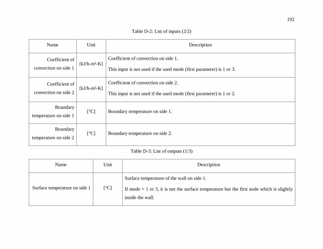
192
Table D-2: List of inputs (2/2)
Name Unit Description
Coefficient of
convection on side 1 [kJ/h-m²-K]
Coefficient of convection on side 1.
This input is not used if the used mode (first parameter) is 1 or 3.
Coefficient of
convection on side 2 [kJ/h-m²-K]
Coefficient of convection on side 2.
This input is not used if the used mode (first parameter) is 1 or 2.
Boundary
temperature on side 1 [°C] Boundary temperature on side 1.
Boundary
temperature on side 2 [°C] Boundary temperature on side 2.
Table D-3: List of outputs (1/3)
Name Unit Description
Surface temperature on side 1 [°C]
Surface temperature of the wall on side 1.
If mode = 1 or 3, it is not the surface temperature but the first node which is slightly
inside the wall.
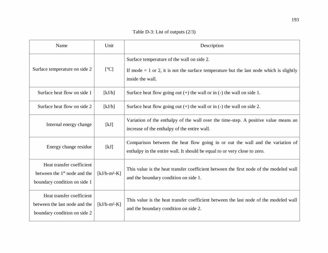
193
Table D-3: List of outputs (2/3)
Name Unit Description
Surface temperature on side 2 [°C]
Surface temperature of the wall on side 2.
If mode = 1 or 2, it is not the surface temperature but the last node which is slightly
inside the wall.
Surface heat flow on side 1 [kJ/h] Surface heat flow going out (+) the wall or in (-) the wall on side 1.
Surface heat flow on side 2 [kJ/h] Surface heat flow going out (+) the wall or in (-) the wall on side 2.
Internal energy change [kJ] Variation of the enthalpy of the wall over the time-step. A positive value means an
increase of the enthalpy of the entire wall.
Energy change residue [kJ] Comparison between the heat flow going in or out the wall and the variation of
enthalpy in the entire wall. It should be equal to or very close to zero.
Heat transfer coefficient
between the 1st node and the
boundary condition on side 1
[kJ/h-m²-K] This value is the heat transfer coefficient between the first node of the modeled wall
and the boundary condition on side 1.
Heat transfer coefficient
between the last node and the
boundary condition on side 2
[kJ/h-m²-K] This value is the heat transfer coefficient between the last node of the modeled wall
and the boundary condition on side 2.

194
Table D-3: List of outputs (3/3)
Name Unit Description
Temperature at the center of
layer “x” [°C] Temperature at the center of each layer (from side 1 to 2).
Temperature at the layers
interface “y” [°C] Temperature at the interface between 2 layers (from side 1 to 2).
Mean liquid fraction of layer
“x” [-]
Mean liquid fraction of each layer (from side 1 to 2). If equal to 0, it is solid. If equal
to 1, it is liquid.


