
1
Modeling Uncertainty in Seismic Imaging of Reservoir Structure
Satomi Suzuki1, Jef Caers1, Robert Clapp2 and Biondo Biondi2 1Department of Petroleum Engineering, Stanford University
2Department of Geophysics, Stanford University
1. Introduction
The modeling of structurally complex reservoirs is one of the most difficult tasks in reservoir
modeling. The difficulty in characterizing complex structural geometry is mainly attributed to the
large uncertainty in seismic images resulting from the limited quality/resolution of seismic data. The
uncertainty in seismic velocity is an example of the source of such uncertainty. Inaccurate seismic
velocity model produces inaccurate migration of seismic images, and consequently, an inaccurate
positioning of fault location/geometry. Despite the structural uncertainty associated with seismic
imaging and the risk in relying on deterministic structural models, reservoir models are rarely
constructed from more than one seismic image. Seismic processing and interpretation are too time
consuming to interpret multiple seismic data sets. Instead, a single processed seismic image is
interpreted. From this single structural interpretation, an uncertainty model is built by perturbing fault
and horizon location (Ref. 1). However, this type of uncertainty analysis completely ignores the
uncertainty of the images itself, which may be of greater importance, in many practical cases, than the
uncertainty modeled from a single structural interpretation. One of the consequences is that, in
structurally complex reservoirs, it is very difficult to obtain a history match of production data,
because the prior structural uncertainty is too small. The location and geometry of faults, which are
known to exert strong impact on fluid flow behavior especially in water (or gas) drive recovery
process, is usually fixed. Other parameters, such as fault transmissibility or facies properties, are then
forced to compensate for the “wrong” structural model. Moreover, poorly identified fault location can
easily mislead future development planning since the distribution of bypassed oil is often controlled
by faults.
A desirable approach for overcoming this problem is a structural uncertainty modeling based on
the uncertainty assessment of seismic imaging. This is achieved by obtaining multiple alternative
seismic images, from which multiple alternative structural models are obtained. Recently, Clapp (2003
Ref.2, 2001 Ref.3) proposed a methodology for assessing the uncertainty in seismic velocity in the
processing of raw seismic data. By accounting for this uncertainty and by inputting multiple velocity
models into the migration of seismic data, multiple seismic data/image sets were obtained. Structural
models interpreted on the resulting multiple seismic images can be used as a set of prior reservoir

2
models for history matching problem, providing prior information on structural uncertainty. By
evaluating posterior structural uncertainty through the incorporation of production data, the fully
integrated assessment of the structural uncertainty would be achieved, hopefully assisting in the risk
evaluation in future development planning. In order to make such an application feasible, an efficient
and robust algorithm for automatic seismic interpretation is required since manual structural
interpretation on dozens of seismic images is usually impossible.
This report outlines a methodology and some preliminary results of the structural uncertainty
modeling proposed by the joint research project between SCRF (Stanford Center Reservoir
Forecasting) and SEP (Stanford Exploration Project). In this paper, we propose a modeling strategy
which consists of 1) obtaining multiple seismic images through the quantification of uncertainty of
seismic velocity, and 2) a new method for automatic seismic interpretation. The creation of multiple
seismic data set is carried out by applying the method of Clapp (Ref. 2). Automatic seismic
interpretation is performed using SIMPAT simulation (Arpat, 2005 Refs. 4~6). Both of the
methodologies are reviewed/discussed in Section 2. Section 3 presents the results of a synthetic
reservoir application.
2. Method
2.1. Multiple Seismic Imaging Assessing Velocity Uncertainty: Review
In this research, the uncertainty in seismic imaging is modeled using the method of Clapp (1-D
super Dix, Ref.2) by focusing on the uncertainty in seismic velocity. This section briefly describes the
methodology of Clapp using the example from Ref.2. Although the methodology is used in a classical
ray-based tomography problem in the original paper (Ref.2), this example explains general application.
The figures shown below demonstrate the typical velocity estimation procedure from CMP gather.
Source: Robert G. Clapp, Multiple realizations and data variance: Successes and failures,
Stanford Exploration Project, Report 113, 2003
two-
way
trav
elti
me
(s),
t
offset (km), h velocity (km/s)
trav
elti
me
dept
h(s)
, τ
trav
eltim
ede
pth
(s),
τ
velocity (km/s)
vRMS(auto-pick)
vint
two-
way
trav
elti
me
(s),
t
offset (km), h velocity (km/s)
trav
elti
me
dept
h(s)
, τ
trav
eltim
ede
pth
(s),
τ
velocity (km/s)
vRMS(auto-pick)
vint

3
The left figure shows an example of CMP gather (traveltime vs. offset) obtained at particular common
midpoint. Assuming waves as expanding circles, the relation between traveltime and offset is
described as:
2RMS
222
v
h4t += τ (1)
t: two-way traveltime (i.e. traveltime from source to receiver)
τ: zero-offset two-way traveltime (called ‘traveltime depth’)
h: offset
vRMS: root-mean-square (RMS) velocity
Assuming a horizontally layered velocity field where the velocity of each layer is defined as interval
velocity (vint), RMS velocity (vRMS) in Eq.(1) is defined as below:
∑
∑
=
=
∆
∆= i
1jj
i
1jj
2jint,
2i,RMS
v
vτ
τ ( )N,.......,2,1i = (2)
∆τ in Eq.(2) is layer thickness in traveltime depth, which is related to physical layer thickness ∆z as:
intv
z2∆=∆τ (3)
Reflector
Source Receiver
∆τ1, vint,1
∆τ2, vint,2
∆τ3, vint,3
∆τ4, vint,4
1
2
3
4
Reflector
Source Receiver
∆τ1, vint,1
∆τ2, vint,2
∆τ3, vint,3
∆τ4, vint,4
1
2
3
4

4
According to Eq.(1), the amplitude shown in the CMP gather is regarded as a collection of hyperbola
curves which are characterized by traveltime depth and corresponding RMS velocity at individual
reflection points. The actual relation between traveltime and offset is not exactly hyperbolic since
wave propagation is not precisely circular in laterally heterogeneous velocity field. However, it is an
usual practice to estimate RMS velocity using this hyperbolic approximation. The velocity scan
(center figure) for estimating RMS velocity is generated from the CMP gather by taking the
summation of amplitude along each hyperbola curve, then plotting that sum in a traveltime depth vs.
RMS velocity plane. On the velocity scan, we observe a peak of strong amplitude responses which
indicates the RMS velocity corresponding to reflection point at traveltime depth τ. The RMS velocity
is estimated as a function of τ by auto-picking the maximum amplitude response on the velocity scan
(dashed line in the center figure). The interval velocity (vint, dashed line in the right figure) is
calculated from the auto-picked RMS velocity using the relationship expressed in Eq.(2).
However, amplitude response peak usually shows considerable spread on the velocity scan, which
indicates that the auto-picked RMS velocity is uncertain. This uncertainty is attributed to the noise of
seismic data and the limited applicability of hyperbolic approximation. Clapp (Ref. 2~3) proposed to
generate equi-probable multiple realizations of the velocity as a function of depth, instead of obtaining
a single best-estimate velocity model. The multiple velocity models are then used to produce equi-
probable migrations of the seismic data. The methodology takes the following procedure.
1) Auto-picking of RMS velocity and evaluation of error variance
The first step is to obtain the RMS velocity from the velocity scan by auto-picking, and to
evaluate the error variance of the RMS velocity from the velocity scan. The error variance σv2(τ) at
traveltime depth τ is evaluated as,
( )( ) ( ){ } ( )
( )∫∫ −
=RMS
4RMS
RMS4
RMS2
pick_auto,RMSRMS2v
dv,vs
dv,vsvv
τ
ττττσ (4)
where vRMS,auto_pick(τ) is the auto-picked RMS velocity at traveltime depth τ, s(τ) is the semblance (=
amplitude stacked along each hyperbola) plotted on the velocity scan. In actual application, σv2(τ) is
calculated in a discretized form of Eq.(4). The example of the evaluated auto-picked RMS velocity
and the square-root of error variance is depicted below.

5
Source: Robert G. Clapp, Multiple realizations and data variance: Successes and failures,
Stanford Exploration Project, Report 113, 2003
2) Construction of the inversion problem
The interval velocity vint is obtained from the auto-picked RMS velocity vRSM using the relation in
Eq.(2). In principle, it is possible to directly solve for vint by inverting the linear system in Eq.(2).
However, in practice, the auto-picked RMS velocity curve shows considerable small scale fluctuation,
often due to noise in the data. Since the interval velocity is a function of derivative of the RMS
velocity, the direct calculation of vint from noisy vRSM by simply relying on the solution of a linear
system would produce an erroneous interval velocity model.
One of the solutions to avoid a solution of Eq.(2), which is noisy, is to add a regularization
constraint to Eq.(2) to smooth the modeled interval velocity. In other words, one tries to obtain an
interval velocity model which has a given desired smoothness and also best fits to the auto-picked
RMS velocity. This is achieved by solving an inversion problem, where as input data the auto-picked
RMS velocity vRSM is used and a target model is the interval velocity vint. This inversion problem is
constructed based on Eq.(2) and also uses the error variance σv2 of Eq.(4) in order to account for the
uncertainty in auto-picked vRSM. This is done as follows:
Eq.(2) is rewritten as follows by specifying ∆τj = ∆τ (constant):
∑=
=i
1j
2jint,
2i,RMS v
i
1v ( )N,.......,2,1i = (5)
Using Eq.(5) as a forward model, the misfit of vRSM,i2 between that obtained from the auto-picked
RMS velocity (data), vRSM,auto_pick,i,, and that derived from the interval velocity to be inverted (model),
vint,i, is evaluated as:
velocity (km/s)
trav
elti
me
dept
h (s
), τ
VRMS, auto_pick
VRMS, auto_pick+σv
VRMS, auto_pick−σv
velocity (km/s)
trav
elti
me
dept
h (s
), τ
VRMS, auto_pick
VRMS, auto_pick+σv
VRMS, auto_pick−σv

6
−=−= ∑∑
==
i
1j
2jint,
2i,pick_auto,RMS
i
1j
2jint,
2i,pick_auto,RMSi vvi
i
1v
i
1vr
( )N,.......,2,1i = (6)
For simplicity, the auto-picked RMS velocity vRSM,auto_pick,i will be denoted as vRSM,i hereafter. The
residual rn,i to be minimized in the inversion problem is defined from the misfit ri (Eq.(6)) and the
error variance σv,i2 (Eq.(4)) as follows:
−== ∑
=
i
1j
2jint,
2i,RMS2
i,v2
i,v
ii,n vvi
i
1rr
σσ ( )N,.......,2,1i = (7)
The minimization of the residual rn,i accounts for the data uncertainty in vRSM,i in obtaining the best-fit
model, i.e., since i,n2
i,vi rr σ= from Eq.(7), a large misfit ri is allowed for a large error variance σv,i2
and vice versa.
Eq.(7) is written in matrix form as,
( )221 CD intRMSn vTvr −Σ= (8)
where:
[ ]N,ni,n2,n1,n r,,r,,r,r KKKK=Tnr
[ ]2N,RSM
2i,RSM
22,RSM
21,RSM v,,v,,v,v KKKK=T2
RSMv
[ ]2Nint,
2iint,
22int,
21int, v,,v,,v,v KKKK=T2
intv
[ ]N,,i,,2,1 KKKK=TT
Σ: diagonal matrix whose diagonal element is 1/σv,i2
D1: diagonal matrix whose diagonal element is 1/Ti
C: lower triangular matrix with the elements of 1 (causal integration)
A regularization term, whose purpose is to generate smooth inverted vint, is added to the problem
as:

7
2D intm vr = (9)
By minimizing rn and rm jointly using the least square optimization, the maximum likelihood
solution of the interval velocity vint is obtained. This is done through the minimization of,
2220 mn rr ε+≈ (10)
where ε is a scaling weight.
3) Generation of multiple realizations of interval velocity
The next step is to generate multiple realizations of interval velocity vint(l) based on the maximum
likelihood model vint(0) obtained from Eq.(10). This is achieved through generating multiple residual
vectors rn(l) which have the same covariance structure as that of the initial residual vector rn
(0) obtained
from ( )2)0(21
)0( CD intRMSn vTvr −Σ= . For this purpose, a filter matrix H is constructed based on a
method of prediction error filter (PEF, see Ref. 8 for details).
The important property of the filter matrix H is: if we apply the filter matrix H to the initial
residual vector rn(0), we obtain white noise vector y(0) as output (see Ref. 8 for proof and method for
obtaining H). Inversely, if we apply the inverse of the matrix H, i.e. H-1, to an arbitrary chosen white
noise vector y(l), we obtain a new residual vector rn(l), which exhibits the same covariance structure as
the initial residual vector rn(0).
Source: Robert G. Clapp, Multiple realizations and data variance: Successes and failures,
Stanford Exploration Project, Report 113, 2003
initial residual rn
White noise
H
H-1
initial residual rnWhite noise
H
H-1

8
Therefore, introducing the filter matrix H, Eq.(8) is rewritten as:
( )221 CDHH intRMSn vTvry −Σ== (11)
The vector y in Eq.(11) is white noise. The multiple realizations of interval velocity vint (l) are
generated by substituting y by a series of randomly chosen white noise vectors y(l), and solving
Eq.(11) for vint. Due to the property of prediction error filter, the covariance structure of the residual
vector is preserved. The corresponding multiple RMS velocity models vRMS(l) are calculated from
vint (l) using Eq.(5).
Using the multiple velocity models vRMS(l), multiple seismic data sets are obtained by migrating
raw seismic data, and then depth-converted using vint (l).
The migration takes considerable CPU time (much greater than any other reservoir modeling
process such as geostatistical or flow simulation). This is because, while geostatistical simulation
operates only on the physical model space (i.e. 3D at most), migration operates both on data and
model space increasing the dimensionality of the problem. For example, a 3D poststack migration
calls for 5-dimensional nested loops and could take several days of CPU time (for each migration).
Adding the uncertainty in velocity to the problem adds one more loop. Furthermore, the volume of
seismic data/image is generally much larger than the volume of reservoir model grid.
2.2. Automatic Seismic Interpretation Using SIMPAT
Aside from the CPU cost of migration, the manual labor cost of seismic interpretation is also one
of the primary factors that prevent the use of multiple seismic data sets from being practical. Since
manual interpretation is time consuming especially when the volume of data is large, it is essential to
automate the interpretation process in order to build dozens of structural models from various seismic
images. Unfortunately, commercially available automatic interpretation tools are hardly applicable for
structurally complicated reservoirs since most algorithms rely on a simple auto-tracking of amplitude
peaks. For that reason, the need for a robust and efficient automatic seismic interpretation method
arises.
Recently, a pattern-based geostatistical sequential simulation (SIMPAT) algorithm was proposed
by Arpat (2005, Ref. 4~6) by constructing reservoir facies models simulating patterns. The algorithm
is designed to simulate facies or petrophysical property model using training image as prior model for
the spatial pattern of the variable being simulated. Although SIMPAT algorithm is originally

9
developed for pattern simulation/conditioning problems for characterizing geological objects such as
fluvial channels, it also has a potential for the application to automatic seismic interpretation problem
by the following reasons.
1) The SIMPAT algorithm is built on multi-scale pattern recognition technique. In fact, this
process is quite similar to horizon/fault picking in manual seismic interpretation process,
since manual horizon picking is done based on visual inspection of the ‘patterns’ of
reflections rather than the mere tracking of amplitude peaks.
2) The similarity evaluation method used in SIMPAT algorithm works better for filtered training
image (Ref. 9). Considering that a seismic amplitude image is virtually an illustration of
naturally filtered horizons, the problem is suitable to SIMPAT algorithm.
Thus we propose to use SIMPAT algorithm as a tool for automatic seismic interpretation. This section
briefly reviews SIMPAT algorithm first, then describes the proposed approach for automatic
interpretation next.
2.2.1 SIMPAT Algorithm with Soft Data Conditioning: Review
The automatic seismic interpretation problem is categorized as a “soft data conditioning” problem
amongst the algorithms covered by SIMPAT. Thus this review focuses on how soft data conditioning
is performed by SIMPAT (Ref. 6).
Consider the problem to simulate fluvial channel using seismic image as conditioning data. This
problem is called “soft data conditioning” problem since the simulated geological object will be
conditioned to the soft (secondary) information from seismic image rather than to the direct (hard)
information such as well observation. The soft data conditioning problem uses a set of two types of
training images, i.e. “hard training image” and “soft training image”. In this example, the hard training
image is an illustration of fluvial channel which describes the desired pattern of channel objects to be
simulated. This hard training image can be taken from geological analog, can be purely conceptual, or
can be an unconditional Boolean realization. The soft training image is a seismic image obtained by
forward-modeling the seismic data on the hard training image. It can be as simple as a moving average
of the hard training image or as complex as the result of full seismic wave modeling.
The patterns of hard variable (e.g. channel object) and soft variable (e.g. seismic amplitude),
which are observed on the hard and soft training images, are related to each other and stored in the
pattern database. An example of pattern database construction is as shown below:

10
Source: Guven Burc Arpat, Sequential simulation with patterns,
Ph.D. Dissertation, 2005
As depicted in the figure, both training images are scanned by a template window to extract the
pattern of objects. The hard image pattern and the soft image pattern extracted at the collocated grid
node are coupled and stored in the pattern database as a pair of hard and soft patterns. Thus the
constructed pattern database can be considered as a training database which stores the information
about pattern-to-pattern correlation observed between hard and soft training image.
Using the constructed pattern database, channel objects are simulated conditioning to actual
seismic data. The actual seismic data is denoted as “soft data” in SIMPAT. The procedure takes
sequential simulation algorithm; i.e., visiting nodes on simulation grid one after another, following a
random path. However, the methodology simulates channel objects as a “pattern” using the template
window, instead of simulating facies in single grid node. The procedure takes the following steps:

11
1. Visit empty grid node u and place the template window there. Extract the pattern of
previously simulated objects within the template window. Denote this (hard) pattern as hd(u).
2. Extract the pattern of the soft data at node u by placing the template window on the
collocated soft data grid. Denote this (soft) pattern as sft(u).
3. Search the pattern database and find a joint pair of hard and soft patterns (hpat, spat) such
that 1) whose hard pattern (hpat) is as similar to hd(u) as possible and 2) whose soft pattern
(spat) is also as similar to sft(u) as possible. The similarity between the patterns a and b,
where a and b are expressed as vectors whose elements are grid values filled in the template
window, is evaluated using Manhattan distance as below:
baba −=,d (12)
The smaller distance ba,d indicates to the greater similarity between a and b. Therefore,
the pair of patterns (hpat, spat) which best matches to hd(u) and sft(u) is found by searching
the pattern database for the pair of (hpat, spat) which shows the minimum value of
( ) ( )usftspat,uhdhpat, dwdw 21 + , for some user-specified weights w1 and w2,
4. Paste the best-matched pattern hpat to the template window location at grid node u.
5. Go to another empty grid node and repeat steps 1~4 until the entire grid is simulated.
The numerous implementation details are discussed in Arpat (Ref.6, 2005). Notice that, at the early
stage of the simulation, a pattern is determined mostly based on the matching of the soft patterns, i.e.
spat and sft(u), since at this stage the previously simulated patterns are few. Thus the algorithm first
draws the rough framework of channel pattern mostly conditioning to the soft data, and then
eventually fills the gaps of simulated patterns accounting for previously simulated objects.
Naturally, a larger template captures the pattern of geological variability better. However, the
large template size requires considerable CPU time, and also requires large size of hard and soft
training images in order to extract large enough numbers of pattern pairs to construct meaningful
pattern database. In order to avoid this problem, SIMPAT algorithm adopts multiple-grid approach
using dual templates: That is, first simulate on coarse grid using a coarse (primal) template, and then
simulate on refined grid using refined (dual) template (See Ref.6 for details).

12
2.2.2 Application of SIMPAT for Automatic Interpretation
The figure shown below schematically illustrates the proposed method for automatic seismic
interpretation using SIMPAT.
As depicted in the figure, we arbitrarily select one seismic image (denoted as ‘image 1’) from the set
of multiple images provided by the method described in Section 2.1. The selected seismic image is
utilized for manual structural interpretation by an expert. This image is termed “soft training image” in
SIMPAT. The result of the manual seismic interpretation (structural model) from the soft training
image is converted to a categorical pixelized image that depicts horizons and faults, and is used as
“hard training image” in SIMPAT. Our goal is to obtain the new structural images from the other
seismic images (image 2~), by conditioning the horizons and faults to the pattern of reflections
observed in these seismic images. This is achieved by performing SIMPAT simulation using new
seismic images (image 2~) as “soft data” together with soft and hard training images.
The advantage of SIMPAT simulation over conventional auto-horizon-picking can be explained
as follows: Since the conventional auto-picking tool merely tracks amplitude peaks to pick horizons, it
does not include any learning process in the automated modeling procedure. However, with SIMPAT,
we use the seismic image and the corresponding structural model as a pair of soft and hard training
images. This training image pair serves as ‘teacher’s interpretation’ which informs how experts
correlate the continuity of amplitude to horizon and discontinuity to faults. Therefore, since SIMPAT
Hard TISoft TI (Image1)
Manual job
Use this for
manual inter-
pretation
Seismic interpretation by an expert
SIMPAT
Soft data (Image2~) Realization
?Other
seismic image
Automatic interpretation by SIMPAT
(Soft data conditioning)
Pattern database
Hard TISoft TI (Image1)
Manual job
Use this for
manual inter-
pretation
Seismic interpretation by an expert
SIMPAT
Soft data (Image2~) Realization
?Other
seismic image
Automatic interpretation by SIMPAT
(Soft data conditioning)
Pattern database

13
simulation is virtually an image processing which is performed by mimicking pattern-to-pattern
correlation tendency that appears on the training image pair, the simulated structural model would be
more realistic than conventional auto-picking result in terms of resemblance to human interpretation.
3. Synthetic Reservoir Application
3.1. Model Description
The synthetic reservoir model used in this study is constructed based on an actual reservoir data
from the North Sea. The model is a two dimensional cross-sectional model consisting 680*340 grid
blocks, 3400m in horizontal direction and 850m in vertical direction. The grid block size is 5m in
horizontal and 2.5m in vertical. The depth of reservoir is 2270 ~ 3120 m-TVDSS. Fig.1 and Fig.2
show the facies distribution and net-to-gross ratio, i.e. (net sand thickness in gridblock)/(gross
gridblock thickness), distribution of the reservoir model. The reservoir is faulted sand stone reservoir
with thin shale layers and tiny calcite bodies (Fig.1). The upper and lower part of the reservoir is shaly
sand while the middle part of the reservoir is clean sand embedded by discontinuous thin calcite
bodies. Porosity and permeability was geostatistically populated with the constraint of geological
maps as depicted in Figs.3 and 4. Average porosity and permeability are 0.24 and 537 mD,
respectively. Water saturation distribution (Fig.5) was modeled with OWC at 2688.5 m-TVDSS and
capillary transition using J-function from the porosity and permeability realization. The fluid densities
are obtained from the field data. The reservoir is modeled as undersaturated reservoir without gas cap.
The water saturation of shale and calcite bodies is specified as 1.0.
The rock physics properties are modeled based on the petrophysical properties model. Fig.6
depicts bulk density model calculated from the porosity and net-to-gross ratio realizations. The fluid
densities are obtained from actual field data (Fig.6). Mineral density and composition for sand and
shale are specified as presented in Fig.6. The density of calcite is taken from literature (Fig.6, Ref.10).
Fig.7 shows a P-wave velocity model generated from the porosity, net-to-gross ratio, and water
saturation realizations. The p-wave velocity of water saturated sand is calculated using empirical
correlation presented in Fig.7 (Han, Ref.10). Gassmann’s relation (Ref.10) was applied for fluid
substitution using bulk modulus obtained from field data and literature value (Fig.7). The P-wave
velocity of shale is calculated using empirical correlation presented in Fig.7 (Gardner, Ref.10). P-
wave velocity of calcite is obtained from the literature (Fig.7, Ref.10). The P-wave impedance model
is computed from bulk density and P-wave velocity and presented in Fig.8. As depicted in Fig.8, shale
layers and calcite bodies are highlighted by high impedance.

14
3.2. Result of Multiple Seismic Imaging and Automatic Seismic Interpretation
A synthetic seismograph is generated from the rock physics property model and utilized for
seismic imaging. Fig.9 depicts the result of multiple seismic imaging obtained by the method of Clapp
(Section 2.1). To create a training interpretation result, the horizon and faults are manually picked on
an arbitrary selected seismic image (image 1) as shown in Figs.10~11. In this particular example, the
boundary between shaly sand/clean sand and that between calcite/clean sand are relatively clear on the
seismic image (Fig.10). We decided to pick positive amplitude peaks to create a training structural
model (Fig.11).
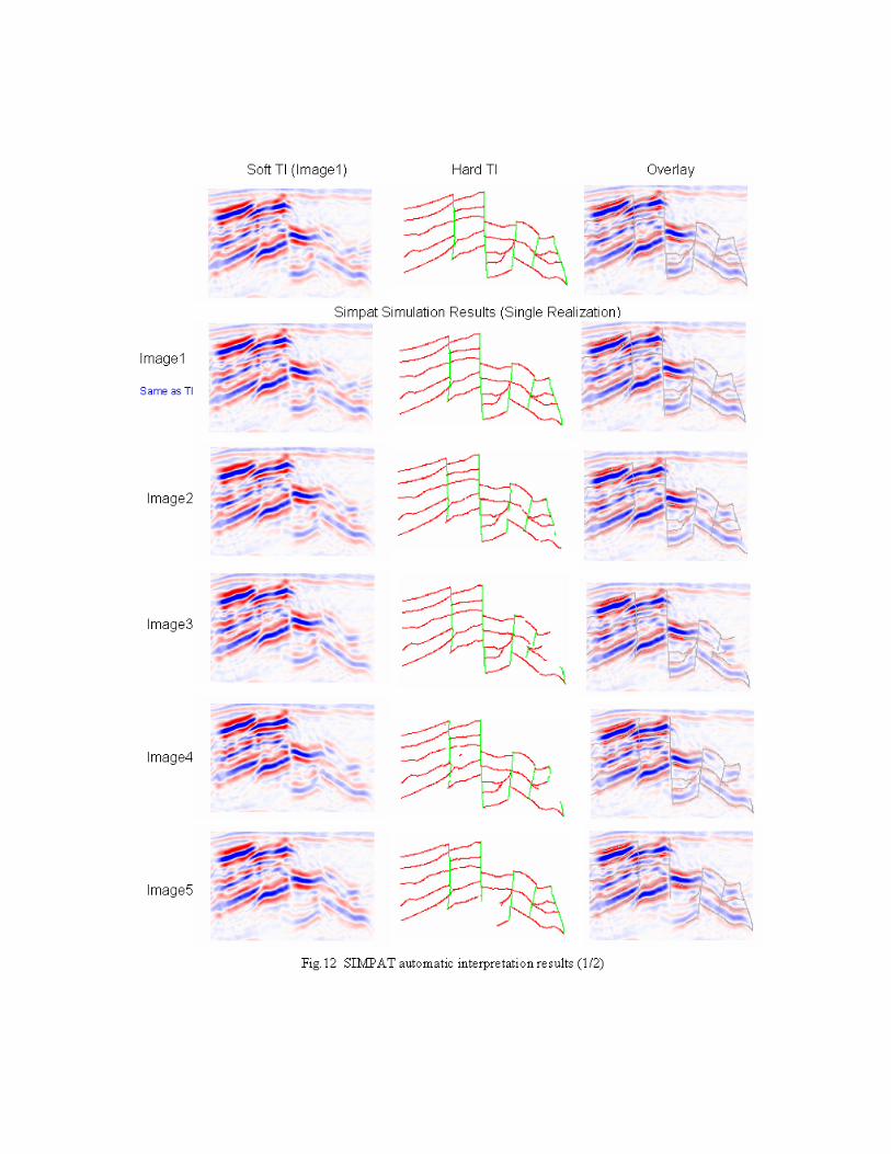
Fig.12 illustrates the result of automatic seismic interpretation with SIMPAT (Section 2.2) using
the manually interpret structural model as a hard training image and also using the seismic image
utilized for manual interpretation (image 1) as a soft training image. The left column shows the
seismic images used as soft data. The center column depicts the simulated horizons and faults. The
right column is the seismic image overlaid by simulated horizons and faults. Shown in the top row is
the soft and hard training images used for simulation. As shown in the figure, the result is quite
encouraging in this simple preliminary application. However, in some images, horizons are partly
missing especially at the zones/compartments where the response of amplitude is relatively weak.
This missing horizon problem is partly attributed to the similarity calculation method (Manhattan
distance) used in SIMPAT algorithm (Ref. 9). The limitation of Manhattan distance is, when applied
to ‘sparse’ training images such as edge image, the evaluated similarity of patterns is biased toward
‘sparser’ patterns. This leads to the underestimation of the continuity of image when applied for
simulating edge images. Arpat suggested to apply distance transformation to categorical training
image in order to avoid this problem (Ref.9). The basic idea is to convert edge images into more
blurred images such as proximity maps (Fig.13) and simulate proximity map instead of simulating
‘sparse’ categorical patterns. The example of proximity maps generated from hard training image (i.e.
faults and horizons) is depicted in Fig.13. The proximity map is practically an opposite to distance
map, thus it is created by calculating the distance to the closest fault or horizon and reversing the
normalized distance to proximity measure. The structural model is obtained by back-transforming the
simulated proximity maps. Fig.14 shows the result of automatic seismic interpretation through the
SIMPAT simulation with distance transformation. As shown in the figure, the reproduction of
connectivity of horizons is improved compared to Fig.13.
The other approach for improving automatic seismic interpretation result is to use an E-type
estimate for creating structural model, instead of using a single simulated realization. An E-type
estimate is obtained from a number of simulated categorical realizations, by calculating the relative
15
frequency of occurrence of the categorical variables at each grid node. Therefore, a map of E-type
estimate can be considered as a probability map which depicts the local conditional probability of
categorical variables. Since automatic seismic interpretation is a pattern conditioning problem rather
than a pattern simulation problem, it is a practical idea to build structural model based on the E-type
estimate from multiple simulation results, since a map of E-type estimate directly illustrates the
likelihood of horizon/fault locations. Fig.15 depicts the E-type estimate of simulated structural image
generated from 5 realizations. Distance transformation is not applied for simulation in this case to see
the effect of the use of E-type. As shown in the figure, the connectivity of horizons is enhanced
compared to Fig.13.
4. Discussion
This paper shows some initial results on creating multiple structural models from multiple seismic
data sets. This paper takes the view that often the most important uncertainty lies in the seismic data
itself, not in the multiple interpretation on a single seismic image. The method consists of generating
multiple seismic data sets by considering the uncertainty in the velocity model and relying on
SIMPAT to automatically interpret the results. Many challenges remain as listed below:
1) Test on seismic data set with more variability
The synthetic seismic data set used in this paper is of good quality. As a result, the obtained
multiple seismic images are similar to each other. Although the automatic seismic interpretation with
SIMPAT showed some encouraging results in this simple and easy problem, it does not guarantee that
one would obtain an equally good result if he/she applies the same approach to more difficult problem
such that the multiple seismic images show more variation from each other. The method requires more
testing using seismic data set with more variability.
2) CPU cost for seismic migration
The CPU time required for the migration of seismic image is also an issue that prevents the
multiple seismic imaging from being practical. Especially, migrating 3D seismic data using dozens of
different velocity models is almost impossible considering the CPU time required. One of the possible
strategies to compromise is to use so called “2.5D model”: That is, migrate the seismic data on
selected 2D cross-sections of 3D seismic data, and construct a fence model of reservoir structure. The

16
final structural model can be obtained by interpolating the horizons and faults between 2D cross-
sectional structural interpretations.
3) Automatic gridding of reservoir structure for flow simulation
A reservoir flow simulation model grid is usually built using commercial geo-modeling/gridding
software, creating model grids from horizon/fault surfaces. In structurally complex reservoirs, it often
requires time-consuming manual job. In order to construct dozens of prior reservoir flow simulation
models for history matching from multiple structural interpretation results, an efficient automatic
gridding method is desired to reduce the required time and labor.
An approach to automatically construct model grid from the automatic seismic interpretation
result is proposed as below:
As shown in the figure, the pixelized structural image generated by SIMPAT is converted into a
compartment model, by grouping the pixels enclosed by the same horizons and faults. The reservoir
model grid is built by overlaying coarse grids on the boundaries between compartments first, and then
subdividing each compartment into fine grids. The example shown in the figure is implemented on 2D
structural model. 3D extension of the method, or application for 2.5D structural model, is required.
4) Parameterization of the structural model for automatic history matching
In automatic history matching, the reservoir parameters to be inverted are expressed in the form of
vector. The optimization is performed by finding the minimum on N-dimensional Cartesian model
space, where N is the dimension of the parameter vector. However, it is difficult to parameterize
structural geometry into a limited set of parameters, especially when the structure is complex, since in
such reservoirs structural geometry is characterized by the topology of horizons and faults rather than
grid data values such as depth of horizon. The history matching approach proposed in this paper
(Section 1) starts from multiple prior structural models defined by the uncertainty in seismic imaging,
and aims at reducing that uncertainty through the incorporation of production data. Since the structural
SIMPAT Result Compartment Model Reservoir Model GridSIMPAT Result Compartment Model Reservoir Model Grid

17
models do not fit to the vector-form model space, a new approach for automatic history matching is
needed.
In the area of computer science, images are often stored in tree data structure in accordance with
similarity distance between images, and tree search algorithm is utilized to find images similar to a
given image in a large collection of images (Ref.11). Several tree structures have been proposed to
maximize the search efficiency. We propose to apply this technique for automatic history matching
problem to find structural models which reproduce historical production data. This idea relies on the
assumption that the similarity of structural geometry between reservoir models is strongly related to
the similarity of production behavior between them. Thus the validity of this assumption should be
carefully tested before implementing the tree-search history matching.
5) Incorporation of probabilistic approach into history matching
One thing to be avoided in the history matching is to select only one structural model which
matches best to the production data, and ignore all other structural models at the stage of future
performance prediction / development planning. Such an application completely ignores structural
uncertainty and waste all of the effort made for modeling the uncertainty in seismic image. Therefore,
the automatic history matching method should be designed such that methodology evaluates the
posterior probability of structural models through the incorporation of production data. In other words,
we should adopt a probabilistic approach to history matching instead of ‘greedy’ optimization
technique. The tree structure used for automatic history matching should be designed to fit to this need.
5. References
1. Magali Lecour, Richard Cognit, Isabelle Duvinage, Pierre Thore and Jean-Claude Dulac,
Modeling of stochastic faults and fault networks in a structural uncertainty study, Petroleum
Geoscience, 2001
2. Robert G. Clapp, Multiple realizations and data variance: Successes and failures, Stanford
Exploration Project, Report 113, 2003
3. Robert G. Clapp, Multiple realizations: Model variance and data uncertainty, Stanford
Exploration Project, Report 108, 2001
4. Burc G. Arpat and Jef Caers, A multi-scale pattern-based approach to stochastic simulation,
SCRF report, 2003
5. Burc G. Arpat, SIMPAT: Stochastic simulation with patterns, SCRF report, 2004
6. Burc G. Arpat, Sequential simulation with patterns, Ph. D dissertation, 2005

18
7. Biondo L. Biondi, 3-D Seismic Imaging, Lecture Note, 2005
8. Jon Claerbout and Sergey Fomel, Image estimation by example: Geophysical soundings
image construction: multidimensional autoregression, Lecture Note & Electronic publishing
(http://sepwww.stanford.edu/sep/prof/index.html), 2004
9. Burc G. Arpat, Training image and distance transformations in SIMPAT, SCRF report, 2005
10. Mavko, Mukerji, and Dvorkin, The rock physics handbook, Cambridge, 1998
11. Sergey Brin, Near Neighbor Search in Large Metric Spaces, Proceedings of the 21st VLDB
Conference, 1995

3400 m
680*340 Blocks, Grid Size: DX = 5 m, DZ = 2.5 m
Fig.1 Facies model
SEAL
3400 m
680*340 Blocks, Grid Size: DX = 5 m, DZ = 2.5 m
Fig.1 Facies model
SEAL

Shale / Calcite NTG = 0.00
3400 m
- 3120 m
- 2270 m
850 m
680*340 Blocks, Grid Size: DX = 5 m, DZ = 2.5 m
Fig.2 Net-to-gross ratio model
Shale / Calcite NTG = 0.00
3400 m
- 3120 m
- 2270 m
850 m
680*340 Blocks, Grid Size: DX = 5 m, DZ = 2.5 m
Fig.2 Net-to-gross ratio model

Shale / Calcite Porosity = 0.001
3400 m
- 3120 m
- 2270 m
850 m
680*340 Blocks, Grid Size: DX = 5 m, DZ = 2.5 m
Fig.3 Porosity model
Shale / Calcite Porosity = 0.001
3400 m
- 3120 m
- 2270 m
850 m
680*340 Blocks, Grid Size: DX = 5 m, DZ = 2.5 m
Fig.3 Porosity model

Shale/Calcite Permeability = 0.001
3400 m
- 3120 m
- 2270 m
850 m
680*340 Blocks, Grid Size: DX = 5 m, DZ = 2.5 m
Fig.4 Permeability model
Shale/Calcite Permeability = 0.001
3400 m
- 3120 m
- 2270 m
850 m
680*340 Blocks, Grid Size: DX = 5 m, DZ = 2.5 m
Fig.4 Permeability model

SHALE/CALCITE
J(Sw)=0.12*(Sw - Swir)^-0.5 - 0.12504071 (phi=0.25, K=500 mD)
H = 31831.6*J(Sw)*TS*(phi/K)^0.5 / (rho_w- rho_o)
OWC = 2688.5 m (from ECLIPSE DATA)
TS = 22 dynes/cm
rho_w = 995 kg/m3 (from ECLIPSE DATA)
rho_o = 730 kg/m3 (from ECLIPSE DATA)
SAND
Sw = 1.00
WATER SATURATION1.0
0.0
0.5
3400 m
- 3120 m
- 2270 m
850 m
680*340 Blocks, Grid Size: DX = 5 m, DZ = 2.5 m
Fig.5 Water Saturation model
SHALE/CALCITE
J(Sw)=0.12*(Sw - Swir)^-0.5 - 0.12504071 (phi=0.25, K=500 mD)
H = 31831.6*J(Sw)*TS*(phi/K)^0.5 / (rho_w- rho_o)
OWC = 2688.5 m (from ECLIPSE DATA)
TS = 22 dynes/cm
rho_w = 995 kg/m3 (from ECLIPSE DATA)
rho_o = 730 kg/m3 (from ECLIPSE DATA)
SAND
Sw = 1.00
WATER SATURATION1.0
0.0
0.5
1.0
0.0
0.5
3400 m
- 3120 m
- 2270 m
850 m
680*340 Blocks, Grid Size: DX = 5 m, DZ = 2.5 m
Fig.5 Water Saturation model

SHALE
Quarts 2.654 0.6 Quarts+Rock frg. 2.642 0.2
Feldspar 2.630 0.3 Clay minerals 2.500 0.8
Rock frg. 2.710 0.1
CLEAN SAND
Rho_b = phi*rho_fl + (1-phi)*rho_m
rho_fl = rho_w *Sw + rho_o*(1-Sw)
SAND/SHALE
rho_m=rho_sand*NTG+rho_sh*(1-NTG)
CALCITE rho_m=2.71
rho_w = 995 kg/m3 (from ECLIPSE DATA)
rho_o = 730 kg/m3 (from ECLIPSE DATA)
Comp.densityComp.density
Mineral composition for rho_sand & rho_sh ( from Stanford V channel sand & mud)
3400 m
- 3120 m
- 2270 m
850 m
680*340 Blocks, Grid Size: DX = 5 m, DZ = 2.5 m
Fig.6 Bulk density model

CALCITE
SAND
Vp = (5.55 - 6.96*phi-2.18C)*1000. (30 MPa, Han, Water saturated rock)
Vs = (3.47 - 4.84*phi-1.87C)*1000. (30 MPa, Han, Water saturated rock), C = 1 - NTG
Fluid Substitution (Gassmann)
Kfl1 = Kwat, Kfl2 = Russ average of Kwat & Koil
Kmin = Russ average of Ksand & Kclay
Kwat = 2.14 GPa, Koil = 0.5 GPa (from ECLIPSE DATA)
Ksand = 39 GPa, Kclay = 25 GPa (from Han)
rhob = 1.75*(Vp/1000.)^0.265 (Gardner 1974)
Vp (m/s)
SHALEVp = 6640 m/s
3400 m
- 3120 m
- 2270 m
850 m
680*340 Blocks, Grid Size: DX = 5 m, DZ = 2.5 m
Fig.7 P-wave velocity model

sand
Imp (m/s-g/cm3)
calcite
shale
3400 m
- 3120 m
- 2270 m
850 m
680*340 Blocks, Grid Size: DX = 5 m, DZ = 2.5 m
Fig.8 P-wave impedance model
sand
Imp (m/s-g/cm3)
calcite
shale
3400 m
- 3120 m
- 2270 m
850 m
680*340 Blocks, Grid Size: DX = 5 m, DZ = 2.5 m
Fig.8 P-wave impedance model

Image 1 Image 2
Image 4Image 3
Image 55
-5
0
Amplitude
Fig.9 Multiple seismic images (1/2)
Image 1 Image 2
Image 4Image 3
Image 55
-5
0
5
-5
0
Amplitude
Fig.9 Multiple seismic images (1/2)

Image 8
Image 6 Image 7
5
-5
0
Amplitude
Image 9
Image 10
Fig.9 Multiple seismic images (2/2)
Image 8
Image 6 Image 7
5
-5
0
5
-5
0
Amplitude
Image 9
Image 10
Fig.9 Multiple seismic images (2/2)

Calcite
Shaly SS
RpρVp
Clean SS
Clean SS
Clean SS
Clean SS
Clean SS
Shaly SS
Shale
Shale
Calcite
Calcite
Shaly SS
Shaly SS
Shaly SS (pinches out)
Shale
Shale
Calcite
Calcite
Clean SS
Clean SS
Clean SS
Clean SS
Clean SS
Shaly SS
Clean SS
Shaly SS
Clean SS
Clean SS
Calcite
Shale
Shaly SS
Shale
Calcite
Clean SS
Clean SS
CalciteShale
Shaly SS
Shale
Clean SS
Calcite
Clean SS
Shaly SS
Clean SS
Clean SS
ShaleShaly SS
Shale
Clean SSCalcite
Clean SS
Clean SS
Shaly SS
Clean SS
Shaly SS
Clean SS
Shale
Shaly SS
Calcite
Clean SSShale
Image 1: Draft interpretation
5
-5
0
Amplitude
Calcite
Shaly SS
RpρVp
Clean SS
Clean SS
Clean SS
Clean SS
Clean SS
Shaly SS
Shale
Shale
Calcite
Calcite
Shaly SS
Shaly SS
Shaly SS (pinches out)
Shale
Shale
Calcite
Calcite
Clean SS
Clean SS
Clean SS
Clean SS
Clean SS
Shaly SS
Clean SS
Shaly SS
Clean SS
Clean SS
Calcite
Shale
Shaly SS
Shale
Calcite
Clean SS
Clean SS
CalciteShale
Shaly SS
Shale
Clean SS
Calcite
Clean SS
Shaly SS
Clean SS
Clean SS
ShaleShaly SS
Shale
Clean SSCalcite
Clean SS
Clean SS
Shaly SS
Clean SS
Shaly SS
Clean SS
Shale
Shaly SS
Calcite
Clean SSShale
Image 1: Draft interpretation
Calcite
Shaly SS
RpρVp
Clean SS
Clean SS
Clean SS
Clean SS
Clean SS
Shaly SS
Shale
Shale
Calcite
Calcite
Shaly SS
Shaly SS
Shaly SS (pinches out)
Shale
Shale
Calcite
Calcite
Clean SS
Clean SS
Clean SS
Clean SS
Clean SS
Shaly SS
Clean SS
Shaly SS
Clean SS
Clean SS
Calcite
Shale
Shaly SS
Shale
Calcite
Clean SS
Clean SS
CalciteShale
Shaly SS
Shale
Clean SS
Calcite
Clean SS
Shaly SS
Clean SS
Clean SS
ShaleShaly SS
Shale
Clean SSCalcite
Clean SS
Clean SS
Shaly SS
Clean SS
Shaly SS
Clean SS
Shale
Shaly SS
Calcite
Clean SSShale
Image 1: Draft interpretation
5
-5
0
5
-5
0
Amplitude
Fig.10 Preliminary manual seismic interpretation
Calcite
Shaly SS
RpρVp
Clean SS
Clean SS
Clean SS
Clean SS
Clean SS
Shaly SS
Shale
Shale
Calcite
Calcite
Shaly SS
Shaly SS
Shaly SS (pinches out)
Shale
Shale
Calcite
Calcite
Clean SS
Clean SS
Clean SS
Clean SS
Clean SS
Shaly SS
Clean SS
Shaly SS
Clean SS
Clean SS
Calcite
Shale
Shaly SS
Shale
Calcite
Clean SS
Clean SS
CalciteShale
Shaly SS
Shale
Clean SS
Calcite
Clean SS
Shaly SS
Clean SS
Clean SS
ShaleShaly SS
Shale
Clean SSCalcite
Clean SS
Clean SS
Shaly SS
Clean SS
Shaly SS
Clean SS
Shale
Shaly SS
Calcite
Clean SSShale
Image 1: Draft interpretation
5
-5
0
Amplitude
Calcite
Shaly SS
RpρVp
Clean SS
Clean SS
Clean SS
Clean SS
Clean SS
Shaly SS
Shale
Shale
Calcite
Calcite
Shaly SS
Shaly SS
Shaly SS (pinches out)
Shale
Shale
Calcite
Calcite
Clean SS
Clean SS
Clean SS
Clean SS
Clean SS
Shaly SS
Clean SS
Shaly SS
Clean SS
Clean SS
Calcite
Shale
Shaly SS
Shale
Calcite
Clean SS
Clean SS
CalciteShale
Shaly SS
Shale
Clean SS
Calcite
Clean SS
Shaly SS
Clean SS
Clean SS
ShaleShaly SS
Shale
Clean SSCalcite
Clean SS
Clean SS
Shaly SS
Clean SS
Shaly SS
Clean SS
Shale
Shaly SS
Calcite
Clean SSShale
Image 1: Draft interpretation
Calcite
Shaly SS
RpρVp
Clean SS
Clean SS
Clean SS
Clean SS
Clean SS
Shaly SS
Shale
Shale
Calcite
Calcite
Shaly SS
Shaly SS
Shaly SS (pinches out)
Shale
Shale
Calcite
Calcite
Clean SS
Clean SS
Clean SS
Clean SS
Clean SS
Shaly SS
Clean SS
Shaly SS
Clean SS
Clean SS
Calcite
Shale
Shaly SS
Shale
Calcite
Clean SS
Clean SS
CalciteShale
Shaly SS
Shale
Clean SS
Calcite
Clean SS
Shaly SS
Clean SS
Clean SS
ShaleShaly SS
Shale
Clean SSCalcite
Clean SS
Clean SS
Shaly SS
Clean SS
Shaly SS
Clean SS
Shale
Shaly SS
Calcite
Clean SSShale
Image 1: Draft interpretation
5
-5
0
5
-5
0
Amplitude
Fig.10 Preliminary manual seismic interpretation


Proximity maps from Hard TI
Faults
Horizons
Fig.13 Distance transformation of hard training image
Proximity maps from Hard TI
Faults
Horizons
Fig.13 Distance transformation of hard training image


Hard TISoft TI (Image1)
E-type (5 Realizations)
Image1
Image2
Image3
Image4
Image5
Same as TI
Fig.15 SIMPAT automatic interpretation results using E-type map, w/o distance transformation (1/2)
Hard TISoft TI (Image1)
E-type (5 Realizations)
Image1
Image2
Image3
Image4
Image5
Same as TI
Fig.15 SIMPAT automatic interpretation results using E-type map, w/o distance transformation (1/2)

Hard TISoft TI (Image1)
Image6
Image7
Image8
Image9
Image10
E-type (5 Realizations)
Fig.15 SIMPAT automatic interpretation results using E-type map, w/o distance transformation (2/2)
Hard TISoft TI (Image1)
Image6
Image7
Image8
Image9
Image10
E-type (5 Realizations)
Fig.15 SIMPAT automatic interpretation results using E-type map, w/o distance transformation (2/2)


