Morava Hopf algebras and spaces K(n)equivalent to finite Postnikov systems
Michael J. Hopkins ∗
Massachusetts Institute of TechnologyCambridge, Massachusetts 02139
Douglas C. Ravenel †
University of RochesterRochester, New York 14627
W. Stephen WilsonJohns Hopkins University
Baltimore, Maryland [email protected]
December 29, 1994
Abstract
We have three somewhat independent sets of results. Our firstresults are a mixed blessing. We show that Morava K-theories don’tsee k-invariants for homotopy commutative H-spaces which are finitePostnikov systems, i.e. for those with only a finite number of homo-topy groups. Since k-invariants are what holds the space together,this suggests that Morava K-theories will not be of much use aroundsuch spaces. On the other hand, this gives us the Morava K-theory ofa wide class of spaces which is bound to be useful. In particular, thiswork allows the recent work in [RWY] to be applied to compute theBrown-Peterson cohomology of all such spaces. Their Brown-Petersoncohomology turns out to be all in even degrees (as is their Morava K-theory) and flat as a BP ∗ module for the category of finitely presentedBP ∗(BP ) modules. Thus these examples have extremely nice Brown-Peterson cohomology which is as good as a Hopf algebra.
∗Partially supported by the National Science Foundation†Partially supported by the National Science Foundation
1
Our second set of results produces a large family of spaces whichbehave as if they were finite Postnikov systems from the point of viewof Morava K-theory even though they are not. This allows us to applythe above results to an even wider class of spaces than finite Postnikovsystems. These examples come from spaces in omega spectra withcertain properties. There are many well known examples with theseproperties. In particular, we compute the K(n) homology of all thespaces in the Ω-spectra for P (q) and k(q) where q > n.
In order to prove our results on finite Postnikov systems we needour third set of results; a beginning of an analysis of bicommutativeHopf algebras over K(n)∗.
Contents
1 Introduction 2
2 Proof of the main theorem 11
3 Strongly K(n)∗-acyclic connective spectra 23
4 Morava homology Hopf algebras 31
1 Introduction
The Morava K-theories are a collection of generalized homology theories
which are intimately connected to complex cobordism ([JW75], [Wur91]).
It is known that they play a central role in aspects of homotopy theory
([Hop87],[DHS88],[HS]). This and their relative computability (due to a
Kunneth isomorphism) makes them a powerful tool. For each prime, p, and
n > 0, the coefficient ring for K(n)∗(−) is K(n)∗ ' Fp[vn, v−1n ] where the
degree of vn is 2(pn − 1).
We assume that all of our spaces are homotopy equivalent to a CW
complex.
2
Theorem 1.1 Let X be a connected p-local space with πk(X) finitely gen-
erated over Z(p), k > 1, and non-zero for only a finite number of k. Then
K(n)∗(ΩX) has a natural filtration by normal sub-Hopf algebras:
K(n)∗ ' F−(n+2) ⊂ · · · ⊂ F−2 ⊂ F−1 ⊂ F0 ' K(n)∗(ΩX)
with
F−q//F−(q+1) ' K(n)∗(K(πq(ΩX), q))
as Hopf algebras.
If K(n)∗(ΩX) is commutative (e.g. if X is an H-space), then K(n)∗(ΩX)
is isomorphic, as a Hopf algebra, to the associated graded object above:
K(n)∗(ΩX) '⊗
0≤m≤n+1
K(n)∗(K(πm(ΩX),m)).
This is natural if either all πk(X), k > 1, are finite, or if they are all free.
We believe that if K(n)∗(X) is not commutative then we still have the
last isomorphism as coalgebras but have been unable to prove it. It may
require a dual Borel theorem for our Hopf algebras and we have only been
able to handle the bicommutative case.
We actually state and prove a theorem (Theorem 2.1) which does not
require the homotopy groups to be finitely generated over Z(p). We can have
copies of Q/Z(p) but our groups can only have a finite number of summands.
This is important both for our proofs and for some of our applications. The
last naturality statement is true in this case if all the homotopy groups are
torsion.
Note also that the n = 0 case of this theorem is a familiar result about
rational homology.
In [MM92], McCleary-McLaughlin show that for an Eilenberg–Mac Lane
space X with finite homotopy group, K(n)∗(X) has the same rank as
K(n− 1)∗(LX), where LX denotes the free loop space of X. In view of
the theorem above, the following generalization of their result is immediate.
3
Corollary 1.2 Let X be a simply connected H-space with finitely many non-
trivial homotopy groups, each of which is finite. Then K(n)∗(X) has the same
rank as K(n− 1)∗(LX).
The following corollary follows from the fact that the Morava K-theory
of Eilenberg–Mac Lane spaces is even degree (except for the circle) and from
the main results of [RWY]. The condition on π1 is needed to avoid having
copies of the circle in our space, giving us odd degree elements.
Corollary 1.3 If X is as in Theorem 1.1 and π1(ΩX) is torsion, then
K(n)∗(ΩX) is even degree and so is BPp∗(ΩX) where BPp is the p-adic
completion of BP . If πk(X) is finite for k > 1 then BP ∗(ΩX) is even
degree. In either case, it is a flat BP ∗-module for the category of finitely
presented BP ∗(BP )-modules.
We see the Morava K-theory cannot distinguish between the double loops
of such a space and a product of Eilenberg–Mac Lane spaces with the same
homotopy groups. One cannot expect to generalize this too much to spaces
with an infinite number of non-zero k-invariants; the sphere, Sk, is a counter
example to that. Inverse limit problems rear their ugly head. Morava K-
theory somehow looks at the whole space rather than how it is put together.
On the other hand, our result certainly does cover spaces with infinitely many
homotopy groups if the k-invariants are zero for all but a finite number of
stages. This is because the Eilenberg–Mac Lane spaces split off as a product if
the k-invariant is zero. Another, more substantial direction of generalization
is to spaces in Ω-spectra with certain stable properties.
Although the abstract isomorphism is interesting from a theoretical point
of view, the practical value comes because the MoravaK-theory of Eilenberg–
Mac Lane spaces is completely known, [RW80]. In particular, it is always even
degree (except for the circle). We also know that
K(n)∗(K(πm(ΩX),m)) ' K(n)∗
4

if m > n + 1, so that Morava K-theory does not see the higher homotopy
groups of these spaces, and spaces with only higher homotopy groups are
acyclic, e.g. if ΩX is n connected and πn+1(ΩX) is torsion. When we have
acyclicity we do not need Hopf algebras much:
Theorem 1.4 Let X an n-connected p-local space with πk(X) a finitely gen-
erated Z(p) module which is non-trivial for only a finite number of k. If
πn+1(X) is torsion, then
K(n)∗(X) ' K(n)∗.
This theorem is rather easy and is proven quite quickly directly from
[RW80].
The proof of Theorem 1.1 is given in Section 2 modulo certain general
results about graded Hopf algebras overK(n)∗ which will be proven in Section
4. It mimics a proof for rational homology. The only place where Section 4
is used is in showing the final statement of Theorem 1.1 about the splitting
as Hopf algebras.
In Section 3, which is independent of the rest of the paper, we will prove
some results about spaces in the Ω-spectrum of a K(n)∗-acyclic spectrum
X. Recall that an Ω-spectrum X = X i has ΩX i+1 = X i. A motivating
example for this study was produced by Richard Kramer’s work computing
K(n)∗(k(q) ∗) when n < q.
Theorem 1.5 Let X = X i be a connective Ω-spectrum of finite type with
bottom cell in dimension 0 and K(n)∗(Xm) ' K(n)∗ for some m. Let X →F be a map to a finite Postnikov system which is an equivalence through
dimension n+ 1. Then X q is K(n)∗-equivalent to F q for all q ≥ 0.
This is Theorem 3.7. We can now apply Theorem 1.1 to such a spectrum
to get:
5

Theorem 1.6 Let X be as in Theorem 1.5, then, for all k ∈ Z,
K(n)∗(X k) '⊗
n+1≥i≥0
K(n)∗(K(πi(X k), i))
as Hopf algebras. In particular, if k > n + 1, then K(n)∗(X k) ' K(n)∗.
Also, if π0(X) is torsion, then X n+1 is K(n)∗-acyclic. Furthermore,
whether K(n)∗(X k) is trivial or not for k ≥ 0 depends only on whether
K(n)∗(K(π0(X), k)) is trivial or not.
We call such a spectrum with one space K(n)∗-acyclic, strongly K(n)∗-
acyclic, because it implies that almost all other spaces are also K(n)∗-acyclic.
We can get the spaces Xm, m > n+ 1 to be K(n)∗-acyclic without reference
to the first section. Note that being strongly K(n)∗-acyclic implies that the
spectrum is K(n)∗-acyclic since K(n)∗(X) = dir limK(n)∗(X k) using the
suspension maps. Bousfield has a generalization of this which may have
useful applications together with the rest of our work. We’ll discuss his
results in Section 3.
This does not lead to a calculation of the Brown-Peterson cohomology
as in the case of a real finite Postnikov system because it is easy to have
spectra which are strongly K(n)∗-acyclic but have non-trivial K(n + 1) ho-
mology. However, following [RWY], it does lead to the calculation of the
E(n) cohomology and a host of others.
What we need now is a condition on X which implies that it is strongly
K(n)∗-acyclic. Associated with the “telescope” conjecture is a functor Lfn,
see [Rav93]. It supplies us with a class of examples. From Corollary 3.13 we
have:
Theorem 1.7 A connective spectrum X for which LfnX is contractible is
strongly K(n)∗-acyclic.
In particular, a suspension spectrum of a finite complex which is K(n)∗-
acyclic is strongly K(n)∗-acyclic. It is possible that the converse of this
6

Theorem is also true. This result is not phrased in the most familiar or
applicable of terms. When X is a BP module spectrum then this functor
coincides with a more familiar one. Let E(n) be the homology theory with
coefficient ring Z(p)[v1, v2, . . . , vn, v−1n ]. We have, from Theorem 3.14:
Theorem 1.8 Let X be a connective BP module spectrum which is
E(n)∗(−)-acyclic, or, equivalently, K(q)∗(−)-acyclic for 0 ≤ q ≤ n, then
X is strongly K(n)∗-acyclic.
What we need now are some concrete examples of interest. This result
can be reduced, Corollary 3.15, to a simpler statement which we can use for
this purpose.
Corollary 1.9 If X is a connective BP -module spectrum in which each el-
ement of π∗(X) is annihilated by some power of the ideal
In+1 = (p, v1, v2, . . . , vn) ⊂ BP∗,
then X is strongly K(n)∗-acyclic.
Thus we see that any connective BP module spectrum with some power
of In+1 mapping to zero is strongly K(n)∗-acyclic. There are a lot of familiar
examples in this collection. Recall that BP∗ ' Z(p)[v1, v2, . . .] where the
degree of vn is 2(pn − 1). We have the spectra BP 〈n〉, with coefficient ring
BP 〈n〉∗ ' Z(p)[v1, v2, . . . , vn], see [Wil75] and [JW73]. We also have P (k, n),
the spectrum with P (k, n)∗ ' BP 〈n〉∗/Ik for 0 ≤ k ≤ n. These theories are
constructed using the usual Baas-Sullivan singularities [Baa73], and [BM71].
Many of these theories are already familiar. In particular, P (0,∞) = BP ,
P (n, n) = k(n), P (k,∞) = P (k), (see [JW75] and [Wur77]), and P (0, n) =
BP 〈n〉. The spaces in the Ω-spectra for P (k, n) are important in studying
the spaces in the Ω-spectra for P (k) in [BW]. In addition, the theories
E(k, n) = v−1n P (k, n), play a prominent role in [RWY].
From the above theorem, we see:
7
Corollary 1.10 For m ≥ q > n, P (q,m) is strongly K(n)∗-acyclic, so, for
k ∈ Z,
K(n)∗(P (q,m)k) '
⊗n+1≥i≥0
K(n)∗(K(πi(P (q,m)k), i)).
We have explicitly computed the K(n) homology of all of the spaces in
the Ω-spectrum for all of these theories. Recall that this includes the more
familiar P (q) and k(q) for q > n. The simplicity of the answer is in stark
contrast with the calculation of K(n)∗(P (n) ∗) in [RW] and of K(n)∗(k(n) ∗)
in [Kra90].
The category of graded Hopf algebras over K(n)∗ is equivalent to that of
Hopf algebras over K(n)∗ ' Fp, graded over Z/(2pn− 2) (where we have set
vn = 1 in order to be working over a perfect field). Not everything about
connected graded Hopf algebras carries over to these Hopf algebras so one
must be somewhat careful. Being careful led us to initiate an investigation of
the type of Hopf algebras that arise when you take the Morava K-theory of
connected homotopy commutative H-spaces. The results of this investigation
may well be of more interest than the applications to finite Postnikov systems
and Section 4 is dedicated to this study.
There, we study what we call commutative Morava homology Hopf al-
gebras (for a given n > 0). These are bicommutative, biassociative, Hopf
algebras over Fp which are graded over Z/2(pn− 1). Furthermore, the prim-
itive filtration is exhaustive and it is the direct limit of finite dimensional Fp
sub-coalgebras. K(n)∗(ΩX), where X is an H-space, is such an object. We
restrict our attention to such objects which are concentrated in even degrees.
Denote this category by EC(n). We show it is an abelian category. For
the sake of completeness, we show that for odd primes the bigger category
splits as EC(n) and OC(n), where OC(n) consists of exterior algebras on
odd degree primitive generators.
Since we deal only with evenly graded objects, our Morava homology
Hopf algebras are really graded over G = Z/(pn − 1). Let H be the cyclic
group of order n. H acts on G via the pth power map. Writing G additively,
8

the map H ×G→ G is given by (i, j)→ pij. Let γ denote an H-orbit:
γ = j, pj, p2j, . . . ⊂ G.
We have:
Theorem 1.11 For each evenly graded commutative Morava homology Hopf
algebra in EC(n), there is a natural splitting
A '⊗γ
Aγ
where the tensor product is over all H-orbits γ and the primitives of Aγ all
have dimensions in 2γ.
To prove this theorem we construct idempotents in our category.
Theorem 1.12 For every A ∈ EC(n) there are canonical idempotents eγ
such that∑γ eγ = 1A and eγeβ is trivial if γ 6= β. These idempotents are
natural. The idempotent eγ sends all primitives to zero which do not have
dimensions in 2γ and is the identity on all primitives which are in dimensions
in 2γ.
Theorem 1.11 follows immediately from this and the fact that tensor
products are the sum in this category. This splitting does even more for
us. Let EC(n)γ be the sub-category of EC(n) whose objects have primitives
only in dimensions in 2γ. What we really prove is the following:
Theorem 1.13 There are commuting idempotent functors, eγ, on EC(n)
such that∑γ eγ is naturally equivalent to the identity functor and eγeβ is the
trivial functor if γ 6= β. As categories:
EC(n) '∏γ
EC(n)γ.
In particular, there is only the trivial map eγ(A) = Aγ → eβ(B) = Bβ if
γ 6= β. Furthermore, EC(n)γ is an abelian category.
9
We can define a function αp : Z/(pn−1)→ Z by just taking the usual lift
to Z and then the usual α, the sum of the coefficients in the p-adic expansion
of our number. αp is constant on an orbit γ. Usually several orbits will have
the same image under the map αp. The following fact is a consequence of the
computations done in [RW80], and is what we need to help prove Theorem
1.1.
Theorem 1.14 In the Hopf algebras K(n)∗(K(T, q)) for any abelian torsion
group T and K(n)∗(K(F, q+1)) for any torsion free abelian group with q ≥ 1,
all orbits γ (as in 1.11) with nontrivial factors satisfy αp(γ) = q.
This is proved below as Theorem 4.14.
Our results were discovered while pursuing the Johnson Question, see
[RW80, Section 13]. This assertion is that if 0 6= x ∈ BPn(X) where X is
a space, then x is not vn torsion. This is a very strong unstable condition.
At present, two of the authors have a good plausibility argument which they
hope to turn into a proof some day. The approach which led to the present
paper was just one of many dead ends. A cohomology theory can be defined
by:
HomBP∗(BP∗(X), Q/Z(p)).
The classifying space for the n-th group, Mn, contains the universal example
for the degree n Johnson Question. In an attempt to get some insight into
its Brown-Peterson homology, the general phenomenon of Theorem 1.1 was
discovered. Each one of these spaces has only a finite number of non-trivial
homotopy groups. Each non-trivial group is a finite sum of copies of Q/Z(p).
Theorem 2.1 still applies to it to give K(n)∗(Mn).
Morava K-theory can sometimes be problematic when p = 2. Because we
are restricted to even degree objects this is not a problem for us, see Remark
4.4.
The authors thank Bill Dwyer, Takuji Kashiwabara, Richard Kramer,
Jim McClure, Jean–Pierre Meyer, Haynes Miller, and Hal Sadofsky, all of
whom helped this project along in one way or another.
10
2 Proof of the main theorem
For a group, G, let R[G] be the group ring for G over R. Let X be the
universal cover for X. We have a sequence of fibrations, up to homotopy:
ΩX → ΩX → π1(X)→ X → X.
Since ΩX and X are connected, we see that
K(n)∗(ΩX) ' K(n)∗(ΩX)⊗
K(n)∗[π1(X)].
From this we see that it is enough to restrict our attention to simply con-
nected spaces; and they all have Postnikov decompositions.
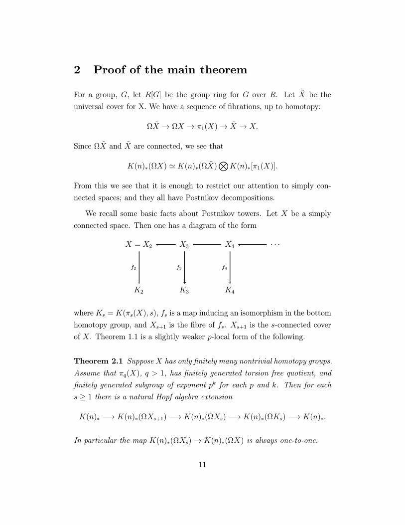
We recall some basic facts about Postnikov towers. Let X be a simply
connected space. Then one has a diagram of the form
X = X2 X3 X4 · · ·
K2 K3 K4
u
f2
u
f3
u
u
f4
u u
where Ks = K(πs(X), s), fs is a map inducing an isomorphism in the bottom
homotopy group, and Xs+1 is the fibre of fs. Xs+1 is the s-connected cover
of X. Theorem 1.1 is a slightly weaker p-local form of the following.
Theorem 2.1 Suppose X has only finitely many nontrivial homotopy groups.
Assume that πq(X), q > 1, has finitely generated torsion free quotient, and
finitely generated subgroup of exponent pk for each p and k. Then for each
s ≥ 1 there is a natural Hopf algebra extension
K(n)∗ −→ K(n)∗(ΩXs+1) −→ K(n)∗(ΩXs) −→ K(n)∗(ΩKs) −→ K(n)∗.
In particular the map K(n)∗(ΩXs)→ K(n)∗(ΩX) is always one-to-one.
11
If X is an H-space, then we have a natural isomorphism of Hopf algebras:
K(n)∗(ΩX) '⊗i≥2
K(n)∗(K(πi(X), i− 1)).
If X is not an H-space, the above isomorphism is still valid additively.
Although this result implies Theorem 1.1 in the Introduction, it is slightly
more general. In particular, it allows for homotopy groups with summands
like Q/Z(p) which we need. The definition of the filtration in Theorem 1.1
comes from the s− 1-connected cover, Xs:
F−s ≡ im K(n)∗(ΩXs) −→ K(n)∗(ΩX).
This filtration is natural. We are not really using the Postnikov construction
of a space, which is not natural, but a Postnikov decomposition which is.
The Postnikov construction starts with a point and builds up the space one
homotopy group at a time. We are starting with the space and taking it
apart one homotopy group at a time. Naturality is clear for the maps on
the Eilenberg–Mac Lane spaces as they are determined by the maps on the
homotopy groups. We want a unique map from Xs+1 to Ys+1 if we inductively
have a unique map from Xs to Ys. The obstruction to uniqueness is in
[Xs+1, K(πs(Y ), s− 1)]
but because Xs+1 is s-connected, this cohomology group is trivial.
Remark 2.2 A number of people have asked us questions about how these
results can be extended. For example, given a fibration of finite Postnikov
systems where the maps all can be delooped several times and the homotopy
groups of the fibre map split-injective to the homotopy groups of the total
space, what can we say about the Morava K-theory of everything? Since we
know the Morava K-theory of all the spaces it seems to us that the results
and techniques used here should answer any question about this situation.
12
In the arguments that follow, it will be convenient to assume that π2(X)
is torsion. In particular, the results of [RW80] imply that K(n)∗(ΩX) is
concentrated in even dimensions in this case. This assumption is harmless
for the following reason. In general (subject to the hypotheses of Theorem
2.1) we have a fibre sequence
X ′ −→ Xf−→ L2
where L2 = K(π2(X)/Torsion, 2) and π2(f) is surjective. Then π2(X ′) is the
torsion subgroup of π2(X), ΩL2 is a finite product of circles, and
ΩX ' ΩX ′ × ΩL2 (2.3)
because we can lift the maps of the circles to homotopy generators using the
H-space structure. Hence it suffices to compute K(n)∗(ΩX′).
The rational case
The corresponding result for rational homology, K(0), is classical and we
will sketch its proof now, since it is a model for the proof of Theorem 2.1.
SinceX has only finitely many nontrivial homotopy groups, Xs is contractible
for large s and we can argue by downward induction on s. Suppose ΩXs+1
has the prescribed rational homology, and consider the fibre sequence
Ω2Ksjs−→ ΩXs+1 −→ ΩXs. (2.4)
For our inductive step we need to prove that
H∗(ΩXs) ' H∗(ΩXs+1)⊗H∗(ΩKs), (2.5)
where all homology groups have rational coefficients. When X is an H-space,
we need the above isomorphism to be one of Hopf algebras. Otherwise it is
an isomorphism of coalgebras.
13

For our calculation we need the bar spectral sequence for a principle
fibration:
F E
B
w
u
(2.6)
which has
E2∗,∗ ' TorK(n)∗(F )
∗,∗ (K(n)∗(E), K(n)∗)⇒ K(n)∗(B). (2.7)
If the fibration we use is the loops on a principle fibration, then the bar
spectral sequence is a spectral sequence of Hopf algebras. Unfortunately, de-
spite a fascination with the bar construction, e.g. [May72], [May75], [Mey84]
and [Mey86], this fact is not in the literature. It can, of course, be patched
up easily from what is there about the standard bar construction. Let our
fibration beΩF ΩE
ΩB
w
u
where (2.6) is a principle fibration. Then ΩF has two products, one from F
and one from the loops. When ΩB is constructed using the bar construction,
one product can be used in the construction and the other can be used to
get a product on the bar construction giving us this spectral sequence as
Hopf algebras (the coalgebra structure is no problem). This works for any
homology theory with a Kunneth isomorphism
In particular, one has the bar spectral sequence converging to H∗(ΩXs)
with
E2 = TorH∗(Ω2Ks)(H∗(ΩXs+1),Q). (2.8)
14
Here the H∗(Ω2Ks)-module structure on H∗(ΩXs+1) is induced by the map
js of (2.4). We have
Lemma 2.9 The map js in (2.4) induces the trivial homomorphism in ra-
tional homology.
Proof. The map js is an H-map, so it must respect the Pontrjagin ring
structure in homology. We know that H∗(Ω2Ks) is generated by elements in
dimension s− 2, while ΩXs+1 is (s− 1)-connected, so H∗(js) is trivial. 2
It follows that (2.8) can be rewritten as
E2 = TorH∗(Ω2Ks)(H∗(ΩXs+1),Q)
= TorH∗(Ω2Ks)(Q,Q)⊗H∗(ΩXs+1)) (2.10)
= H∗(ΩKs)⊗H∗(ΩXs+1))
The rational homology bar spectral sequence collapses for Eilenberg–
Mac Lane spaces and has no extension problems, which explains the last step
above. Now it follows formally that the spectral sequence collapses, because
differentials must lower filtration by at least 2, but H∗(ΩXs+1)) is concen-
trated in filtration 0, and H∗(ΩKs) is generated by elements in filtration 1.
Thus one gets the desired extension of Hopf algebras
Q −→ H∗(ΩXs+1) −→ H∗(ΩXs) −→ H∗(ΩKs) −→ Q. (2.11)
If X is an H-space, then so is Xs, so H∗(ΩXs) is bicommutative. The struc-
ture of graded connected bicommutative Hopf algebras over Q is well known
(see [MM65, Section 7]). In particular, we have the following splitting theo-
rem.
15
Theorem 2.12 Let A be a graded connected bicommutative Hopf algebra
over Q. Then there is a canonical Hopf algebra isomorphism
A '⊗k>0
Ak
where Ak is generated by primitive elements in dimension k. Moreover, Ak
is a polynomial algebra for k even and an exterior algebra for k odd.
It follows that the extension (2.11) is split when X is an H-space and the
rational case of Theorem 2.1 is proved.
The Morava K-theory case for torsion spaces
Now we will give the proof of Theorem 2.1 under the additional assump-
tion that π∗(X) is all torsion. The general setup is the same as in the rational
case. The Morava K-theory of Eilenberg–Mac Lane spaces was computed in
[RW80]. We have the bar spectral sequence as in the rational case, and we
have the following analog of Lemma 2.9.
Lemma 2.13 The map js in (2.4) induces the trivial homomorphism in
Morava K-theory. (Here we do not require that π∗(X) be all torsion.)
Proof. (See the introduction for K(n)∗(−).) We will make use of Theorems
1.11 and 1.14. We are studying the map
K(n)∗(Ω2Ks)
K(n)∗(js)−−−−−→ K(n)∗(ΩXs+1).
Recall that we are using downward induction on s so we can assume Theorem
2.1 for all t > s. Assume our map is nontrivial. Choose the largest t so that
its image is contained in K(n)∗(ΩXt). Then the composition
K(n)∗(Ω2Ks) −→ K(n)∗(ΩXt) −→ K(n)∗(ΩXt)//K(n)∗(ΩXt+1) = K(n)∗(ΩKt)
16
must be nontrivial. This is a Hopf algebra map, and both the source and
target are subject to the splitting theorem 1.11, with the constraints imposed
by 1.14. The factors of K(n)∗(Ω2Ks) correspond to orbits γ with αp(γ) =
s− 2 or s− 3, while those of K(n)∗(ΩKt) have αp(γ) = t− 1 or t− 2. These
orbits are distinct since s < t ≤ n + 1. Since there are no nontrivial Hopf
algebra homomorphisms between factors corresponding to distinct orbits, the
result follows. 2
It follows that the analog of (2.10) holds, namely, in the bar spectral
sequence,
E2 = TorK(n)∗(Ω2Ks)(K(n)∗, K(n)∗)⊗K(n)∗(ΩXs+1).
Now, TorK(n)∗(Ω2Ks)(K(n)∗, K(n)∗) is the E2-term of the bar spectral se-
quence converging to K(n)∗(ΩKs), and this was completely determined in
[RW80]. There is a map to this spectral sequence from the one we are study-
ing, given by the following commutative diagram, in which each row is a fibre
sequence.
Ω2Ks ΩXs+1 ΩXs
Ω2Ks pt. ΩKs
w
js
u
=
w
u u
w w
In our spectral sequence (the one for the top row) the extra factor of
K(n)∗(ΩXs+1) is concentrated in the even degrees (by induction) of filtration
0. In a spectral sequence of Hopf algebras the basic differentials must go from
generators to primitives, see [Smi70, page 78]. In the bar spectral sequence,
differentials must start in filtration greater than one. All generators here
are in even degrees and so must go to odd degree primitives, all of which
are in filtration one [RW80, Theorem 11.5]. So, the start and finish of the
generating differentials are all in the part which maps isomorphically to the
bottom row. It follows that in our spectral sequence,
E∞ = E0K(n)∗(ΩKs)⊗K(n)∗(ΩXs+1),
17
where E0K(n)∗(ΩKs) denotes the E∞-term of the lower spectral sequence,
which was determined in [RW80]. In particular, our E∞-term is concentrated
in even dimensions.
Again the edge homomorphism gives us the desired Hopf algebra exten-sion, namely
K(n)∗ −→ K(n)∗(ΩXs+1) −→ K(n)∗(ΩXs) −→ K(n)∗(ΩKs) −→ K(n)∗. (2.14)
The following result is where we need the assumption that π∗(X) is tor-
sion.
Lemma 2.15 When X is an H-space with torsion homotopy, the extension
(2.14) is split naturally.
Proof. We use Theorems 1.11 and 1.14, and assume inductively that
K(n)∗(ΩXs+1) is as advertised. This means that its factors under Theorem
1.11 all correspond to orbits γ with αp(γ) ≥ s, while those of K(n)∗(ΩKs)
with αp(γ) = s−1. Thus Theorem 1.13 assures us that the extension is split
naturally. 2
Notice that the proof above would fail if the torsion subgroup of πs(X)
and the torsion free quotient of πs+1(X) were both nontrivial, because in that
case, both K(n)∗(ΩXs+1) and K(n)∗(ΩKs) could have factors corresponding
to the same orbit γ. In particular, there is a short exact sequence of Hopf
algebras,
Fp → K(n)∗(K(Z/(pi), j))→ K(n)∗(K(Z(p), j + 1))pi→ K(n)∗(K(Z(p), j + 1))→ Fp,
which shows how maps can drop filtration (from −j to −(j + 1)). This
example prevents us from having a natural Hopf algebra splitting in general.
We do have an unnatural splitting for the general case however, and we
produce that now.
18
Removing the torsion condition
We have given the proof of Theorem 2.1 in the case when π∗(X) is all
torsion. We needed the torsion condition to get the desired Hopf algebra
structure when X is an H-space. We did not need it to show that K(n)∗(ΩXs)
is a subalgebra of K(n)∗(ΩX). Now we will describe an alternate approach
to the Hopf algebra question which does not require π∗(X) to be torsion.
We need to use the rationalization XQ of X. For an H-space (more
generally, a nilpotent space), Y , one has a fibre sequence
TY −→ Y −→ YQ
where π∗(YQ) = π∗(Y )⊗Q and π∗(TY ) is all torsion. For a p-local H-space
Y (such as ΩX(p)), YQ is the homotopy direct limit of
Y[p]−→ Y
[p]−→ Y[p]−→ · · ·
where [p] is the H-space pth power map. In this case YQ and TY are both
H-spaces.
Now for X as in Theorem 2.1, we have a fibre sequence
Ω2XQ −→ ΩTXi−→ ΩX. (2.16)
Before we can proceed, we need to bring in the generalized Atiyah–
Hirzebruch spectral sequence, see [Dol62] and [Dye69]. For a fibration like
(2.6), we have the Atiyah–Hirzebruch–Serre spectral sequence:
E2 ' H∗(B;K(n)∗(F )) =⇒ K(n)∗(E). (2.17)
The map ofE toB maps this spectral sequence to the usual Atiyah–Hirzebruch
spectral sequence:
19

E2 ' H∗(B;K(n)∗) =⇒ K(n)∗(B). (2.18)
Lemma 2.19 If π2(X) ⊗Q = 0, then the map i of (2.16) induces an iso-
morphism in K(n)∗ for all n > 0.
As remarked above (2.3), this assumption on π2(X) can be made without
loss of generality.
Proof of Lemma 2.19. We will use the Atiyah–Hirzebruch spectral sequence
for Morava K-theory to compute K(n)∗(ΩTX). We have the following com-
mutative diagram in which each row is a fibre sequence.
Ω2XQ ΩTX ΩX
pt. ΩX ΩX
w
u
w
i
u
i
u
=
w w
=
(2.20)
The hypothesis on π2(X) implies that Ω2XQ is path connected. We know
that any rational loop space is a product of rational Eilenberg–Mac Lane
spaces. From [RW80, Corollary 12.2] we have
dir limK(n)∗(K(Z/(pi), q)) ' K(n)∗(K(Z, q + 1)). (2.21)
We see that iterating [p] on the left kills everything, so the product of
rational Eilenberg–Mac Lane spaces has the Morava K-theory of a point.
This means that the left vertical arrow in (2.20) is a K(n)∗-equivalence. The
right vertical map is a homology equivalence (since it is the identity map) so
we get an isomorphism of Atiyah–Hirzebruch–Serre spectral sequences, so i
is a K(n)∗-equivalence. 2
20
Now the torsion case of Theorem 2.1 tells us that
K(n)∗(ΩTX) '⊗i≥2
K(n)∗(K(πi(TX), i− 1)),
and this is K(n)∗(ΩX) by Lemma 2.19. Thus Theorem 2.1 will follow from
Lemma 2.22 For a simply connected space X with π2(X) torsion,⊗i≥2
K(n)∗(K(πi(X), i− 1)) '⊗i≥2
K(n)∗(K(πi(TX), i− 1)).
as Hopf algebras.
Proof. There is a split short exact sequence
0 −→ πi+1(X)⊗Q/Z −→ πi(TX) −→ Tor1(πi(X),Q/Z) −→ 0.
Note that Tor1(πi(X),Q/Z) is the torsion subgroup of πi(X), while πi+1(X)⊗Q/Z is the tensor product of Q/Z with the torsion free quotient of πi+1(X).
With this in mind, we also have a split short exact sequence
0 −→ Tor1(πi(X),Q/Z) −→ πi(X) −→ πi(X)/Torsion −→ 0.
According to (2.21)
K(n)∗(K(Z, i+ 1)) ' K(n)∗(K(Q/Z, i)) for i ≥ 1,
so we have
K(n)∗(K(πi+1(X)⊗Q/Z, i− 1)) ' K(n)∗(K(πi+1(X)/Torsion, i)).
It follows that⊗i≥2
K(n)∗(K(πi(TX), i− 1))
=⊗i≥2
K(n)∗(K(πi+1(X)⊗Q/Z, i− 1))
21
⊕⊗i≥2
K(n)∗(K(Tor1(πi(X),Q/Z), i− 1))
=⊗i≥2
K(n)∗(K(πi+1(X)/Torsion, i))
⊕⊗i≥2
K(n)∗(K(Tor1(πi(X),Q/Z), i− 1))
=⊗i≥2
K(n)∗(K(πi(X)/Torsion, i− 1))
⊕⊗i≥2
K(n)∗(K(Tor1(πi(X),Q/Z), i− 1))
=⊗i≥2
K(n)∗(K(πi(X), i− 1)).
2
Remark 2.23 The above process lost us our naturality in the splitting, but
not if all of the homotopy groups are free or torsion. The problems only come
up if we try to mix them.
Proof of Theorem 1.4. First let us assume that πn+1(X) = πn+2(X) = 0.
Theorem 1.1 tells us that K(n)∗(ΩX) is trivial and our result follows from
the bar spectral sequence.
Remark 2.24 We do not have to use Theorem 1.1 here at all. We can do
our downward induction on the Postnikov system directly. Everything will
be trivial so there is no difficulty showing the maps are also trivial and the
spectral sequence is trivial. One can just use Lemma 3.3 over and over again.
We use this result several times in our study of spectra; the point is that those
results are independent of Theorem 1.1.
Next we consider the case where πn+1(X) = 0. If πn+2(X) = 0 or is
torsion, the same proof works. It is only if πn+2(X) has copies of Z(p) in it
that we could have a problem. We take our usual fibration with map:
22

ΩKn+2 Xn+3 X
ΩKn+2 pt. Kn+2.
w
u
=
w
u u
w w
Since πn+1(Xn+3) = πn+2(Xn+3) = 0, we have K(n)∗(Xn+3) is trivial.
Thus we get an isomorphism on the E2 terms of the two bar spectral se-
quences. Thus the E∞ terms must be isomorphic as well. However, since we
know, from [RW80, Theorem 12.3], that
TorK(n)∗(K(Z(p),n+1))(K(n)∗, K(n)∗) = K(n)∗,
we get our result.
All we have left to deal with is the case where πn+1(X) is finite. The
argument is exactly the same as that just given except that the Tor is trivial
by [RW80, Theorem 11.5]. 2
3 Strongly K(n)∗-acyclic connective spectra
Throughout this section n will be assumed to be positive. For a connective
spectrum X, X m for m ≥ 0 will denote the mth space in the associated
Ω-spectrum. Be alert to our (unusual) convention that X m have its bottom
cell in dimension m.
Definition 3.1 A connective spectrum X is strongly K(n)∗-acyclic if Xm
is K(n)∗-acyclic for some m ∈ Z.
One might guess that any K(n)∗-acyclic spectrum is strongly K(n)∗-
acyclic, but we we will see below, (3.9), that this is not the case. We will
23
show, Theorem 3.7, that for such an X each space X m is K(n)∗-equivalent
to a suitable finite Postnikov system.
Remark 3.2 We take a moment to show that we need not restrict ourselves
to positive spaces in the Ω-spectrum, such as in Theorem 1.6. If m ≥ 0, then
we see from the bar spectral sequence that X m K(n)∗-acyclic implies X m+1
is K(n)∗-acyclic. If we have a negative number, write X −m. Let X〈m+ 1〉be the stable m-connected cover of X. Then we have a stable cofibration:
ΣmX〈m+ 1〉 −→ X −→ F
where F is a finite Postnikov system and we have X〈m+ 1〉0
= X −m. If
this is K(n)∗-acyclic, then X〈m+ 1〉k
is K(n)∗-acyclic for all k ≥ 0. We
have an unstable fibration
F k−1 −→ X〈m+ 1〉m+k−→ X k.
For big k, F k−1 is also K(n)∗-acyclic by Theorem 1.4, so X k is K(n)∗-acyclic
by the next lemma.
Lemma 3.3 Let
Fi−→ E
j−→ B
be a fibration with F K(n)∗-acyclic. Then the map j is a K(n)∗-equivalence.
Proof. There is an Atiyah–Hirzebruch–Serre spectral sequence, (2.17), con-
verging to K(n)∗(E) with
E2 = H∗(B;K(n)∗(F )).
It maps to the usual Atiyah–Hirzebruch spectral sequence converging to
K(n)∗(B). Since F is K(n)∗-acyclic, this map is an isomorphism, giving
the desired result. 2
24

Proposition 3.4 Let m ≥ 0, X be a connective spectrum with Xm K(n)∗-
acyclic, and let Y be any connective spectrum. Then (X ∧ Y )m
is also K(n)∗-
acyclic.
Recall here that our convention is that Xm and (X ∧ Y )m
have the same
connectivity.
Proof. We will argue by skeletal induction on Y . Assume for simplicity that
the bottom cell of Y is in dimension 0, so the 0-skeleton Y 0 is a wedge of
spheres. Thus (X ∧ Y 0)m
is a product of Xms and is therefore K(n)∗-acyclic.
For k > 0 consider the cofibre sequence
Σ−1X ∧ Y k/Y k−1 −→ X ∧ Y k−1 −→ X ∧ Y k,
which we abbreviate by A → B → C. Now Am+k−1 (which may be con-
tractible) is K(n)∗-acyclic by a similar argument, and we can assume induc-
tively that Bm is K(n)∗-acyclic. We have a fibration
Am+k−1i−→ Bm
j−→ C m
and Cm is K(n)∗-acyclic by 3.3. This is true for all k > 0, so (X ∧ Y )m
is K(n)∗-acyclic as claimed because it is the direct limit of K(n)∗-acyclic
spaces. 2
We need a standard result which we include here for completeness.
Lemma 3.5 Let X be a connective spectrum and H be the integral Eilenberg–
Mac Lane spectrum. Then X ∧H is the product of Eilenberg–Mac Lane spec-
tra.
Proof. We argue by skeletal induction. We have
Σ−1Xk/Xk−1 ∧H −→ Xk−1 ∧H −→ Xk ∧H.
25
By induction we have Xk−1∧H is the product of Eilenberg–Mac Lane spectra
with homotopy H∗(Xk−1; Z). The first term is just a bunch of Σk−1Hs and so
factors through K(Hk−1(Xk−1), k − 1) in the second term so the third term
is as claimed. 2
Now we can get some control over the connectivity m.
Lemma 3.6 Let X be a connective strongly K(n)∗-acyclic spectrum with
bottom cell in dimension 0. Then the space X n+3 is K(n)∗-acyclic.
Proof. We assume that all spectra and spaces in sight are localized at the
prime p. Let H denote the integer Eilenberg–Mac Lane spectrum, and let H
denote the fibre of the map S0 → H.
H −→ S0 −→ H
The bottom cell of H is in dimension q − 1, where q = 2(p − 1). Thus the
cofibre sequence
Σ−1X ∧H −→ X ∧H −→ X
gives a fibre sequence
(X ∧H)m−1
i−→ (X ∧H)m+q−1
j−→ X m.
(Recall our convention!) Now (X ∧H)m−1
is an (m− 2)-connected product
of Eilenberg–Mac Lane spaces, so it is K(n)∗-acyclic for m−1 > n+ 1. Thus
j is a K(n)∗-equivalence for m ≥ n+ 3. Iterating this argument we see that
X n+3 is K(n)∗-equivalent to (X ∧H(s))n+3+s(q−1)
for each s > 0. The latter
is K(n)∗-acyclic for some s by Proposition 3.4, so X n+3 is also K(n)∗-acyclic.
2
We can use this lemma to prove the following.
26
Theorem 3.7 Let X be a connective strongly K(n)∗-acyclic spectrum with
bottom cell in dimension 0. Let X → F be a map to a finite Postnikov
system which is an equivalence through dimension n+1. Then X m is K(n)∗-
equivalent to F m for all m ≥ 0. In particular, X n+2 is K(n)∗-acyclic, and
if π0(X) is torsion, X n+1 is K(n)∗-acyclic.
Proof. Stably we have a fibre sequence
X ′ −→ X −→ F
where X ′ is a connected cover of X having bottom cell above dimension n+1.
Consider the fibre sequence
F m−1 −→ X ′m′ −→ X m
(where m′ > m+n+1 depends on the connectivity of X ′). From Theorem 1.4
we know that F is strongly K(n)∗-acyclic. Since X is also strongly K(n)∗-
acyclic we can use Lemma 3.3 to see that X ′m′ is also strongly K(n)∗-acyclic.
Hence X ′ n+3 is K(n)∗-acyclic by Lemma 3.6.
Now consider the fibre sequence
X ′m′i−→ Xm
j−→ F m.
For positive m, m′ > m + n + 1 ≥ n + 2, so X ′m′ is K(n)∗-acyclic. By
Lemma 3.3, j is a K(n)∗-equivalence as claimed. In particular, X n+2 is
K(n)∗ equivalent to F n+2, which by Theorem 1.4 is K(n)∗-acyclic. Since
X was arbitrary strongly K(n)∗-acyclic, we also know that X ′ n+2 is K(n)∗-
acyclic, so j is also a K(n)∗-equivalence for m = 0. 2
Pete Bousfield has generalized this in more than one way. His results
are not restricted to Morava K-theories and he does not need to work with
Ω-spectra. In a short note to us he derived these results from [Boua]. More
recently, these have been made explicit in [Boub, Section 7]. Restricting our
attention to Morava K-theories, his result of interest to us is:
27
Theorem 3.8 (Bousfield) An (n+2)-connected H-space Y is K(n)∗-acyclic
if and only if ΩY is K(n)∗-acyclic.
The following example shows that not all connective K(n)∗-acyclic spec-
tra are strongly K(n)∗-acyclic.
Example 3.9 Let X be the spectrum BP 〈n− 1〉 from [Wil75] and [JW73]
for n > 1. The third author showed in [Wil75] that Xm has torsion free
homology and therefore is not K(n)∗-acyclic for m = 2(pn−1)/(p−1). This
would contradict Lemma 3.6 if X were strongly K(n)∗-acyclic, so it is not.
It is, however, K(n)∗-acyclic. This can be seen most easily by considering
the exterior Hopf algebra on the Milnor Bockstein, Qn, as a sub-Hopf algebra
of the cohomology
H∗(BP 〈n− 1〉; Z/(p)) ' A/A(Q0, Q1, . . . , Qn−1).
Then, by Milnor–Moore, 4.4, [MM65], H∗(BP 〈n − 1〉; Z/(p)) is free over
E(Qn−1) and the first differential in the Atiyah–Hirzebruch spectral sequence
for K(n)∗(BP 〈n−1〉) kills everything and we find BP 〈n−1〉 is K(n)∗-acyclic.
Theorem 3.10
(i) Let X → Y → Z be a cofibre sequence of connective spectra. If any
two of X, Y and Z are strongly K(n)∗-acyclic, then so is the third.
(ii) Any retract X of a connective strongly K(n)∗-acyclic spectrum Y is
also strongly K(n)∗-acyclic.
(iii) Any connective direct limit X of connective strongly K(n)∗-acyclic spec-
tra is strongly K(n)∗-acyclic.
Proof. (i) is an easy consequence of Lemma 3.3. For (ii) note that X m is a
retract of Y m′ for suitable m′. For (iii) we can assume that each spectrum
in the direct system has bottom cell in dimension ≥ 0, so Y n+2 is a direct
limit of K(n)∗-acyclic spaces. 2
28
We have so far produced no examples of strongly K(n)∗-acyclic spectra
other than finite Postnikov systems.
Proposition 3.11 Any finite K(n)∗-acyclic spectrum X is strongly K(n)∗-
acyclic.
Proof. X is a suspension spectrum of a (connected) finite complex Y , so for
some m, X m = QY , where
QY = lim−→k
ΩkΣkY.
Since K(n)∗(Y ) ' K(n)∗(X), Y is K(n)∗-acyclic. All we have to do is show
that Y K(n)∗-acyclic implies that QY is K(n)∗-acyclic. There is a stable
splitting, [Sna74], for QY . Each piece of this stable splitting is identified
explicitly as something called e[C(j),Σj , Y ] from [May72, Proposition 2.6(ii),
page 14]. Since C(j) is contractible, [May72, page 5], this is the same as
DΣjY ; for which there is a spectral sequence, [CLJ76, Corollary 2.4, page 7]:
E2 ' H∗(Σj;K(n)∗(Y(j)))⇒ K(n)∗(DΣjY )
where Y (j) is the jth smash product. For reduced Morava K-theory,
K(n)∗(Y(j)) = 0 because we have a Kunneth isomorphism. Thus each piece
of the stable splitting is K(n)∗-acyclic and we have that QY is K(n)∗-acyclic.
This is well known to those familiar with this but, to a novice, perhaps a bit
difficult to dig out of [Sna74]. 2
Corollary 3.12 Any connective spectrum which is a direct limit of finite
K(n)∗-acyclic spectra is strongly K(n)∗-acyclic.
Proof. This follows immediately from Theorem 3.10 and Proposition 3.11. 2
Now recall the localization functors Ln of [Rav84] and Lfn of [Rav93].
The former is Bousfield localization with respect to E(n), while the latter is
constructed in such a way that the fibre of the map X → Lfn is a direct limit
of finite K(n)∗-acyclic spectra. Thus we get
29
Corollary 3.13 A connective spectrum X for which LfnX is contractible is
strongly K(n)∗-acyclic.
Proof. Since LfnX is contractible, the fibre of the map X → Lfn is equivalent
to X. Since X is a connective spectrum which is now the direct limit of finite
K(n)∗-acyclic spectra, X is strongly K(n)∗-acyclic by Corollary 3.12. 2
There is a natural transformation λn : Lfn → Ln. The telescope con-
jecture, which is known to be false for n = 2, see [Rav] and [Rav92b], is
equivalent to the assertion that λn is an equivalence. It is shown that for
n = 2 there is a spectrum X for which LnX is contractible but LfnX is not.
It is necessarily a torsion spectrum (its rational homology must vanish) and
its connective cover has the same property. However we do not know if such
a spectrum is strongly K(n)∗-acyclic or not.
We also know of no counterexample to the converse of Corollary 3.13,
so perhaps that is an equivalence. Alternatively, one can ask if a connective
spectrum X is strongly K(n)∗-acyclic if and only if E(n)∗(X) = 0. In [Rav84,
Theorem 2.1(d)] it was shown that E(n)∗(X) = 0 if and only if K(i)∗(X) = 0
for 0 ≤ i ≤ n. It is also known, [JY80], that E(n)∗(X) = 0 if and only if
v−1n BP∗(X) = 0.
The following is a consequence of Corollary 3.13.
Theorem 3.14 If X is a connective spectrum with E(n)∗(X) = 0, then
BP ∧ X is strongly K(n)∗-acyclic. In particular if X is also a BP -module
spectrum then it is strongly K(n)∗-acyclic. The same holds with BP replaced
by any connective spectrum E with Bousfield class dominated by that of BP .
Proof. By the smash product theorem [Rav92a, 7.5.6], E(n)∗(X) = 0 if and
only if X ∧ LnS0 is contractible. We also know [Rav93, Theorem 2.7(iii)]
that LnS0 and LfnS
0 are BP∗-equivalent and therefore E∗-equivalent. Thus
we have
pt. ' E ∧X ∧ LnS0 ' E ∧X ∧ LfnS0 ' Lfn(E ∧X)
30
(the last equivalence is Theorem 2.7(ii) of [Rav93]) and E ∧ X is strongly
K(n)∗-acyclic by Corollary 3.13. If E is a ring spectrum and X is an E-
module spectrum, then it is a retract of E ∧X,
X ' S0 ∧X −→ E ∧X −→ X
so it is strongly K(n)∗-acyclic by Theorem 3.10(ii). 2
Corollary 3.15 If X is a BP -module spectrum in which each element of
π∗(X) is annihilated by some power of the ideal
In+1 = (p, v1, v2, · · · vn) ⊂ BP∗,
then X is strongly K(n)∗-acyclic.
Proof. The hypothesis implies that v−1n π∗(X) = 0, so v−1
n BP∗(X) = 0,
which is equivalent to E(n)∗(X) = 0 as noted above. 2
Examples of spectra satisfying these hypotheses include the P (k) of
[JW75] (with π∗(P (k)) = BP∗/Ik) for k > n and spectra obtained from
BP 〈k〉 by killing an ideal containing some power of In+1.
4 Morava homology Hopf algebras
We want to study a category of Hopf algebras which includes the objects of
our interest: the Morava K-theory (homology) of homotopy commutative,
connected H-spaces. We need this study to solve Hopf algebra extension
problems in the bar spectral sequence during the inductive step of the proof
of our main theorem. To do this we have a general Hopf algebra splitting
theorem which is of interest in its own right. We want to give particular
thanks to Hal Sadofsky for help with this section.
Although our Hopf algebras will be bicommutative, and so give an abelian
category, we can run into serious problems because of the cyclical grading
31
we use. In particular, we can have an element with the property x = xp. (In
K(n)∗(K(Z/(p), n)) for example.) This wreaks havoc with all of the algebra
portion of Milnor–Moore [MM65]. Such an algebra has no generator (i.e.,
indecomposable), and the first proposition of Milnor–Moore is false for our
situation. The coalgebra portion of Milnor–Moore fares much better. Before
we move on to Hopf algebras we want to indicate why our coalgebras are
still nice by making some definitions and reproving a basic result which still
holds in our setting.
Let A be a cocommutative, coassociative, coaugmented coalgebra with
counit over a ring, R. At present we are not concerned with gradings so
this could be ungraded, graded or cyclically graded. To avoid unnecessary
complications, we assume that A is flat over R. Let J(A) be the cokernel of
the coaugmentation map:
0→ R→ A→ J(A)→ 0.
Using the iterated coproduct we define an increasing filtration, FqA, by
FqA = kerA→ J(A)⊗q+1
for all q ≥ 0. Note that F0A ' R and F1A/F0A ' P (A), the primitives of A.
We call this the primitive filtration of A. Dualizing Milnor–Moore, [MM65,
page 252], we could call this the coaugmentation filtration. (Milnor and
Moore reserve the name primitive filtration for their filtration on primitively
generated Hopf algebras.)
Following [Boa81] we say a filtration, F∗A, is exhaustive (or exhausts A)
if every element of A is in some FqA. We say A is a (connected) homology
coalgebra if A is a cocommutative, coassociative, coaugmented coalgebra
over R with counit, its primitive filtration exhausts A, and it is the direct
limit of finite dimensional R sub-coalgebras. The exhaustive condition on A
replaces connectivity in the graded case quite nicely. To justify the name we
have the following observation:
Lemma 4.1 Let E∗(−) be a multiplicative homology theory and X a con-
nected CW complex of finite type such that E∗(X) is flat over E∗, then E∗(X)
32

is a homology coalgebra over E∗.
Proof. Because E∗(X) is flat over E∗, the Kunneth isomorphism holds for
finite products of X. The diagonal, X → X ×X, induces a cocommutative,
coassociative coalgebra over E∗. The map of a point into X (because X is
connected) and the map of X to a point give the coaugmentation and counit
respectively. Again, we need connectivity to show the primitive filtration is
exhaustive. An element of E∗(X) which lives on the 0-cell maps trivially
to J(E∗(X)). Since E∗(X) is the direct limit of E∗(Xq) where Xq is the q-
skeleton, any element x in E∗(X) comes from E∗(Xq) for some q (this shows
the coalgebra is the direct limit of finite dimensional E∗ sub-coalgebras).
Getting a cellular approximation to the iterated diagonal map, X → ∏q+1X
we see that on some coordinate Xq maps to the 0-cell and thus our element
must be in FqE∗(X) and the primitive filtration is exhaustive. 2
We can also prove a standard result which, as we see, does not depend
on a grading, but just on having an exhaustive primitive filtration. This is
well known and is even somewhere in the algebraic topology literature but
we cannot remember where we have seen it. In the other literature, it could
well be that Lemma 11.0.1 on page 217 of [Swe69] could prove it; but it is a
lot easier to reprove it than to be sure of that.
Lemma 4.2 Let A → B be a map of coalgebras where A is a homology
coalgebra, then the map injects if and only if the induced map on primitives
injects.
Proof. Since P (A) ⊂ A, an injection on A is automatically an injection on
P (A). In the other direction our proof is by induction on the degree of the
primitive filtration of an element. We are given that P (A) ' F1A injects to
ground our induction. If we have an element, x ∈ FqA but not in Fq−1A,
then the coproduct takes x to∑x′⊗x′′ in J(A)⊗J(A) where each non-zero
x′ and x′′ must be in a lower filtration and so they inject to J(B)⊗ J(B). 2
33
We say that A is a (connected) homology Hopf algebra if it is an asso-
ciative Hopf algebra with unit such that the coalgebra structure is that of a
homology coalgebra. Clearly, if our X above is an H-space, then E∗(X) is a
homology Hopf algebra. If the algebra structure is commutative, we say A is
a commutative homology Hopf algebra . If X above is a homotopy commu-
tative H-space (e.g. any double loop space) then E∗(X) is a commutative
homology Hopf algebra.
Since the exhaustive condition replaces connectivity so nicely, we can
define a Hopf algebra conjugation on homology Hopf algebras. This is done
inductively on the primitive filtration. Let x → x ⊗ 1 + 1 ⊗ x +∑x′ ⊗ x′′,
then C(x) = −x − x′C(x′′) inductively. Following [MM65, Proposition 8.8,
page 260], we have C C = IA because our coalgebra is cocommutative. The
existence of C is essential to show that commutative homology Hopf algebras
are an abelian category, see [Gug66]. We are in a slightly generalized situation
over the usual connected bicommutative Hopf algebras of finite type so it is
worth a short discussion of our case. If A is a coalgebra and B is an algebra,
then two maps from A to B can be combined to get a third, still following
[MM65, Section 8], by
A→ A⊗ Af⊗g−−−−−→ B ⊗B → B.
To get an abelian category we need Hom(A,B) to be an abelian group. In
particular, the above map must be a Hopf algebra map. For A→ A⊗ A to
be a Hopf algebra map, A must be cocommutative. For B ⊗B → B to be a
Hopf algebra map, B must be commutative. So, we need the bicommutativ-
ity of commutative homology Hopf algebras to get our composition back in
our category. The Hopf algebra conjugation above gives us our inverse and
bicommutativity shows Hom(A,B) is an abelian group. Following [MM65,
Sections 3 and 4], bicommutativity allows us to define, for all f : A → B, a
kernel
A\\f ' R2BA ' A2BR
and a cokernel
B//f ' R⊗A B ' B ⊗A R.
34

Tensor product is the product in our category and given maps f : A → B
and g : A → C, we get (f, g) : A → A ⊗ Af⊗g−→ B ⊗ C. The rest of the
conditions to be an abelian category are easy to verify.
Theorem 4.3 The category of commutative homology Hopf algebras is abelian.
In the graded connected case over a perfect field of characteristic p, com-
mutative homology Hopf algebras of finite type have been classified nicely
in [Sch70]. This applies to the case where E is standard mod p homology
theory. Unaware of Schoeller’s work, the second author had also embarked
on such a project. His project was aborted when he learned about Schoeller’s
paper and the only physical remains of this project are in [Rav75]. His ap-
proach was quite different from hers and quite easily extends to the case at
hand, so we are now reaping the benefits of his study in this paper.
What concerns us here are what we will call commutative Morava ho-
mology Hopf algebras. These are just commutative homology Hopf algebras
over Fp which are cyclically graded over Z/(2(pn − 1)) for some n. These
arise naturally when you take the Morava K-theory, K(n)∗(X), where X is
a connected homotopy commutative H-space, and set vn equal to one as we
do throughout the rest of this paper. We do only what we need with these
Hopf algebras here, but we hope to return to the problem of classifying them
in a future paper. Because of the cyclic grading there is a much richer, more
interesting collection of Hopf algebras than in the standard case. The Morava
K-theory of Eilenberg–Mac Lane spaces in [RW80] supplies lots of examples
unlike anything seen in the normal graded case.
Remark 4.4 At this stage we must point out a problem and its solution for
the prime p = 2. K(n) is not a homotopy commutative ring spectrum for
p = 2, so K(n)∗(X) is not necessarily in our category. However, if K(n)∗(X)
is even degree it is. For a discussion of this problem see the Appendix of
[JW82] where, following [Wur77], [RW80] is shown to hold for p = 2.
35
Because of the cyclic grading, it is not unusual to find ourselves dealing
with infinite dimensional vector spaces; for example, a polynomial algebra
with one primitive generator already gets us into that situation. However,
we can use finiteness when we need it because our coalgebras are the direct
limit of finite dimensional sub-coalgebras. Many Hopf algebra categories are
self dual, an extremely nice property. Unfortunately, ours is not self dual.
We can define the dual category, however.
Proposition 4.5 Let A be a commutative homology Hopf algebra over a field
R. It is the direct limit of its finite dimensional subcoalgebras Aα. Let its
dual be defined by
A∗ = lim←
HomR(Aα, R).
Then A∗ is a compact topological bicommutative Hopf algebra under the in-
verse limit topology. Moreover A is the continuous linear dual of A∗.
Proof. The product and coproduct in A∗ are induced respectively by the
coproduct and product in A. A∗ is compact because it is the inverse limit
of finite dimensional vector spaces. The continuous linear dual of an inverse
limit is the direct limit of the continuous linear dual, and
HomR(HomR(Aα, R), R) = Aα
so the continuous linear dual of A∗ is A. 2
This result enables us to make the following definition.
Definition 4.6 Let A be a commutative homology Hopf algebra over Fp. The
Frobenius map F : A → A is the Hopf algebra homomorphism that sends
each element to it pth power. The Verschiebung map V : A → A is the
dual of the Frobenius map on A∗
We are ready to look closely at the category of commutative Morava
homology Hopf algebras and say what we need to say about it. We propose
36
to split up every Hopf algebra into canonical components. Because it is
all we need for this paper, we restrict our attention to evenly graded Hopf
algebras. Thus our Morava Hopf algebras are really graded over G = Z/(pn−1). Denote by EC(n) the category of evenly graded commutative Morava
homology Hopf algebras (for a given n). Let H be the cyclic group of order
n. H acts on G via the pth power map. Writing G additively, the map
H ×G→ G is given by (i, j)→ pij. Let γ denote an H-orbit:
γ = j, pj, p2j, . . . ⊂ G.
Recall Theorem 1.11 from the introduction, which uses these definitions.
Remark 4.7 We illustrate the result with the case p = 2 and n = 3. Then
H and G have orders 3 and 7 respectively and there are three orbits, namely
γ1 = 1, 2, 4,γ2 = 3, 6, 5 and
γ3 = 0.
We also know, from [RW80], that for i = 1, 2 or 3, K(3)∗(K(T, i)) has its
primitives in dimensions in 2γi for any torsion abelian group T .
We discuss this more later, but in general, K(n)∗(K(T, i)) can have fac-
tors with generators in more than one orbit. For example when p = 2, n = 4
and i = 2 there are two such orbits, namely 3, 6, 9, 12 and 5, 10. How-
ever each orbit is associated with a unique value of i, namely i = αp(j), the
sum of the digits of the p-adic expansion of any j ∈ γ.
Theorem 1.12 follows from Theorem 1.13 by:
Proof of Theorem 1.12. All we need to prove here, after we see how our
functors are constructed, is that there are no non-trivial maps Aγ → Bβ if
γ 6= β. Such a map, f , must commute with eβ which is the identity on Bβ
but is the trivial map on Aγ and so it must be the trivial map. 2
37
Proof of Theorem 1.13. Our concern for the rest of this section is to construct
the idempotents eγ and prove Theorem 1.13. A Hopf algebra, A, in EC(n)
is equipped with the usual Frobenius and Verschiebung endomorphisms F
and V (see 4.6). The relation, V F = FV = p, is a simple calculation. Do
not confuse this p with multiplication by p. This is p times the identity in
the abelian group of endomorphisms of A. Thus the ring of endomorphisms
of A which ignores the grading is a module over Z(p). Because the primitive
filtration is exhaustive every element of A is annihilated by some power of V
and hence by some power of p. This means that the endomorphism ring is
also a module over the p-adic integers Zp.
Given an element a ∈ Fp we can define an endomorphism [a] of A to be
multiplication by ai in dimension 2i. If we replace A by A ⊗ Fpn, we have
an endomorphism [a] for each a ∈ Fpn . Hence the endomorphism ring of
A⊗Fpn is a module over Zp[G], the p-adic group ring over G = Z/(pn − 1),
which is isomorphic to the multiplicative group of the field Fpn .
Remark 4.8 Although our applications in this paper only require us to study
evenly graded Hopf algebras, our study of these Hopf algebras would be in-
complete without splitting the category into evenly graded Hopf algebras and
exterior Hopf algebras on odd degree generators for odd primes. Classical sign
arguments force a Hopf algebra with odd degree primitives to be an exterior
algebra. The idempotents necessary for this splitting are just ([1]± [−1])/2.
To check this we need only evaluate on primitives. ([1]− [−1])/2 is the iden-
tity on odd primitives and trivial on even primitives. The reverse is true for
([1] + [−1])/2.
We want to use Zp[G] to construct idempotents of A. We need some
basic facts to do this. Let M be an R module and let H act on R and M .
Then we have a map j : R → End(M) and H acts on f ∈ End(M) by
(hf)(x) = h(f(h−1(x))). Then
Lemma 4.9 If the map j is H-equivariant then the fixed points, RH act on
the fixed points MH .
38

Proof. If m ∈MH and r ∈ RH then
(jr)(m) = (jh(r))(m) = [h(jr)](m) = h(jr(h−1m)) = h(jr(m)).
2
We have our group H = Z/(n). H is isomorphic to the Galois group of
Fpn over Fp, and its action on the ring Zp[G] corresponds to the action of
the Galois group on the units of Fpn . We will write G multiplicatively from
now on. We want to show that if an element x ∈ Zp[G] is fixed by this action
then the corresponding endomorphism leaves A = (A ⊗ Fpn)H ⊂ A ⊗ Fpn
invariant. Hence the endomorphism ring of A is a module over the fixed
point subring Zp[G]H . By our lemma, we must just show that the map
Zp[G] → End(A ⊗ Fpn) is H-equivariant. It is enough to show this on [g].
Let a ∈ A and z ∈ Fpn. Then:
j(h([g]))(a⊗ z) = j([gph
])(a⊗ z)= a⊗ gph|a|z= h(a⊗ g|a|z1/ph)
= h(j[g])(a⊗ z1/ph)
= h(j[g])h−1(a⊗ z).
We construct some idempotents in an even bigger ring, W (Fpn)[G], where
W (Fpn) denotes the Witt ring of Fpn, i.e., the extension of Zp obtained by
adjoining a primitive (pn−1)th root of unity ω. See [Haz78, page 132, Remark
17.4.18]. We will use the notation ω for both the root of unity in W (Fpn)
and its mod p reduction in Fpn . For each j ∈ G let
ej =∑
1≤i≤pn−1
ω−ij[ωi]
pn − 1. (4.10)
Note that ej is independent of the choice of the primitive root ω. One sees
easily that the ej are orthogonal idempotents, i.e.,
ejej′ =
ej if j = j′
0 otherwise(4.11)
39
and∑j
ej = 1.
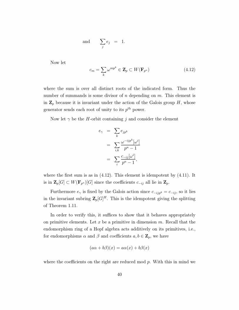
Now let
cm =∑k
ωmpk ∈ Zp ⊂ W (Fpn) (4.12)
where the sum is over all distinct roots of the indicated form. Thus the
number of summands is some divisor of n depending on m. This element is
in Zp because it is invariant under the action of the Galois group H, whose
generator sends each root of unity to its pth power.
Now let γ be the H-orbit containing j and consider the element
eγ =∑k
ejpk
=∑i,k
ω−ijpk[ωi]
pn − 1
=∑i
c−ij[ωi]
pn − 1,
where the first sum is as in (4.12). This element is idempotent by (4.11). It
is in Zp[G] ⊂W (Fpn)[G] since the coefficients c−ij all lie in Zp.
Furthermore eγ is fixed by the Galois action since c−ijpk = c−ij, so it lies
in the invariant subring Zp[G]H . This is the idempotent giving the splitting
of Theorem 1.11.
In order to verify this, it suffices to show that it behaves appropriately
on primitive elements. Let x be a primitive in dimension m. Recall that the
endomorphism ring of a Hopf algebra acts additively on its primitives, i.e.,
for endomorphisms α and β and coefficients a, b ∈ Zp, we have
(aα+ bβ)(x) = aα(x) + bβ(x)
where the coefficients on the right are reduced mod p. With this in mind we
40
have
eγ(x) =∑i
c−ij[ωi](x)
pn − 1
=∑i
c−ijωimx
pn − 1
=∑i,k
ωim−ijpkx
pn − 1
=∑k
(∑i
ωi(m−jpk)
pn − 1
)x.
The inner sum is 1 when m = jpk and 0 otherwise, so we have
eγ(x) =
x if m ∈ γ0 otherwise
as desired. 2
In the introduction we defined a function αp : Z/(pn − 1)→ Z by taking
the sum of the coefficients of the p-adic expansion. We observed that αp is
constant on orbits γ. From Theorem 1.13, we have:
Corollary 4.13 Let EC(n)q =∏αp(γ)=q EC(n)γ for all 0 ≤ q ≤ n(p − 1).
Then:
EC(n) =∏
0≤q≤n(p−1)
EC(n)q.
This is now what we need for our Hopf algebras. We actually need very
little knowledge about K(n)∗(K(Z/(pi), q)). We remind the reader that
K(n)∗(X) ≡ K(n)∗(X)⊗K(n)∗ Fp
where the K(n)∗ module structure of Fp is given by sending vn to 1. The
following is a restatement of Theorem 1.14.
41

Theorem 4.14 ([RW80]) K(n)∗(K(Z/(pi), q)) is in EC(n)q for 0 < q ≤n, and is K(n)∗ ' Fp for q > n. K(n)∗(K(Z(p), q + 1)) is the direct limit of
K(n)∗(K(Z/(pi), q)) and is also in EC(n)q.
Proof. The theorem is read off from [RW80, Theorem 11.1] where we see the
primitives are all in degrees 2(pi1 +pi2 + . . .+piq), 0 = i1 < i2 < · · · < iq < n,
for Z/(pi) and [RW80, Corollary 12.2] for Z(p). In fact, all primitives come
from K(n)∗(K(Z/(p), q)). 2
References
[Baa73] N. A. Baas. On bordism theory of manifolds with singularities.
Math. Scand., 33:279–302, 1973.
[BM71] N. A. Baas and I. Madsen. On the realization of certain modules
over the Steenrod algebra. Math. Scand., 31:220–224, 1971.
[Boa81] J. M. Boardman. Conditionally convergent spectral sequences.
Johns Hopkins University preprint, 1981.
[Boua] A. K. Bousfield. Localization and periodicity in unstable homotopy
theory. Journal of the American Mathematical Society. To appear.
[Boub] A. K. Bousfield. Unstable localization and periodicity. preprint.
[BW] J. M. Boardman and W. S. Wilson. Unstable splittings related to
Brown–Peterson cohomology. in preparation.
[CLJ76] F. R. Cohen, T. Lada, and J.P.May. The Homology of Iterated Loop
Spaces, volume 533 of Lecture Notes in Mathematics. Springer–
Verlag, New York, 1976.
[DHS88] E. Devinatz, M. J. Hopkins, and J. H. Smith. Nilpotence and stable
homotopy theory. Annals of Mathematics, 128:207–242, 1988.
42

[Dol62] A. Dold. Relation between ordinary and extraordinary homol-
ogy. In Colloquium on Algebraic Topology, Aarhus 1962, pages
2–9, 1962.
[Dye69] E. Dyer. Cohomology Theories. Benjamin, New York, 1969.
[Gug66] V. K. A. M. Gugenheim. Cohomology theory in the category of
Hopf algebras. Colloque de Topologie, Centre Belge de Recherches
Mathematiques, pages 137–148, 1966.
[Haz78] M. Hazewinkel. Formal Groups and Applications. Academic Press,
New York, 1978.
[Hop87] M. J. Hopkins. Global methods in homotopy theory. In J. D. S.
Jones and E. Rees, editors, Homotopy Theory: proceedings of the
Durham Symposium 1985, volume 117 of London Mathematical So-
ciety Lecture Note Series, pages 73–96, Cambridge, 1987. Cam-
bridge University Press.
[HS] M. J. Hopkins and J. H. Smith. Nilpotence and stable homotopy
theory II. Annals of Mathematics. To appear.
[JW73] D. C. Johnson and W. S. Wilson. Projective dimension and Brown–
Peterson homology. Topology, 12:327–353, 1973.
[JW75] D. C. Johnson and W. S. Wilson. BP–operations and Morava’s
extraordinary K–theories. Mathematische Zeitschrift, 144:55–75,
1975.
[JW82] D. C. Johnson and W. S. Wilson. The Brown–Peterson homology of
elementary p-groups. American Journal of Mathematics, 102:427–
454, 1982.
[JY80] D. C. Johnson and Z. Yosimura. Torsion in Brown-Peterson ho-
mology and Hurewicz homomorphisms. Osaka Journal of Mathe-
matics, 17:117–136, 1980.
43

[Kra90] R. Kramer. The periodic Hopf ring of connective Morava K-theory.
PhD thesis, Johns Hopkins University, 1990.
[May72] J. P. May. The geometry of iterated loop spaces, volume 271 of
Lecture Notes in Mathematics. Springer–Verlag, Berlin, 1972.
[May75] J. P. May. Classifying spaces and fibrations, volume 155 of Memoirs
of the American Mathematical Society. American Mathematical
Society, Providence, Rhode Island, 1975.
[Mey84] J.-P. Meyer. Bar and cobar constructions, I. Journal of Pure and
Applied Algebra, 33:163–207, 1984.
[Mey86] J.-P. Meyer. Bar and cobar constructions, II. Journal of Pure and
Applied Algebra, 43:179–210, 1986.
[MM65] J. W. Milnor and J. C. Moore. On the structure of Hopf algebras.
Annals of Mathematics, 81(2):211–264, 1965.
[MM92] J. McCleary and D. A. McLaughlin. Morava k-theory and the free
loop space. Proceedings of the American Mathematical Society,
114:243–250, 1992.
[Rav] D. C. Ravenel. A counterexample to the telescope conjecture. To
appear.
[Rav75] D. C. Ravenel. Dieudonne modules for Abelian Hopf algebras. In
D. Davis, editor, Reunion Sobre Teoria de homotopia, Universi-
dad de Northwestern, Agosto 1974, number 1 in Serie notas de
matematica y simposia, pages 177–194, Mexico, D.F., 1975. So-
ciedad Matematica Mexicana.
[Rav84] D. C. Ravenel. Localization with respect to certain periodic ho-
mology theories. American Journal of Mathematics, 106:351–414,
1984.
44

[Rav92a] D. C. Ravenel. Nilpotence and periodicity in stable homotopy the-
ory, volume 128 of Annals of Mathematics Studies. Princeton Uni-
versity Press, Princeton, 1992.
[Rav92b] D. C. Ravenel. Progress report on the telescope conjecture. In
N. Ray and G. Walker, editors, Adams Memorial Symposium on
Algebraic Topology Volume 2, volume 176 of London Mathematical
Society Lecture Note Series, pages 1–21, Cambridge, 1992. Cam-
bridge University Press.
[Rav93] D. C. Ravenel. Life after the telescope conjecture. In P. G. Goerss
and J. F. Jardine, editors, Algebraic K-Theory and Algebraic Topol-
ogy, volume 407 of Series C: Mathematical and Physical Sciences,
pages 205–222. Kluwer Academic Publishers, 1993.
[RW] D. C. Ravenel and W. S. Wilson. The Hopf ring for P (n). in
preparation.
[RW80] D. C. Ravenel and W. S. Wilson. The Morava K–theories
of Eilenberg–Mac Lane spaces and the Conner–Floyd conjecture.
American Journal of Mathematics, 102:691–748, 1980.
[RWY] D. C. Ravenel, W. S. Wilson, and N. Yagita. Brown-Peterson
cohomology from Morava K-theory. in preparation.
[Sch70] C. Schoeller. Etude de la categorie des algebres de Hopf commuta-
tives connexes sur un corps. Manuscripta Math., 3:133–155, 1970.
[Smi70] L. Smith. Lectures on the Eilenberg–Moore spectral sequence, vol-
ume 134 of Lecture Notes in Mathematics. Springer–Verlag, 1970.
[Sna74] V. Snaith. Stable decomposition of ΩnΣnX. Journal of the London
Mathematical Society, 7:577–583, 1974.
[Swe69] M. E. Sweedler. Hopf algebras. Benjamin, New York, 1969.
45
[Wil75] W. S. Wilson. The Ω–spectrum for Brown–Peterson cohomology,
Part II. American Journal of Mathematics, 97:101–123, 1975.
[Wur77] U. Wurgler. On products in a family of cohomology theories as-
sociated to the invariant prime ideals of π∗(BP ). Commentarii
Mathematici Helvetici, 52:457–481, 1977.
[Wur91] U. Wurgler. Morava K-theories: A survey. In S. Jackowski,
B. Oliver, and K. Pawaowski, editors, Algebraic topology, Poznan
1989: proceedings of a conference held in Poznan, Poland, June
22-27, 1989, volume 1474 of Lecture Notes in Mathematics, pages
111–138, Berlin, 1991. Springer–Verlag.
46


![POSTNIKOV TOWERS, -INVARIANTS AND OBSTRUCTION THEORY FOR ... · arXiv:0805.4483v1 [math.KT] 29 May 2008 POSTNIKOV TOWERS, k-INVARIANTS AND OBSTRUCTION THEORY FOR DG CATEGORIES GONC¸ALO](https://cdn.vdocuments.net/doc/165x107/5b15b6497f8b9a45448dac1f/postnikov-towers-invariants-and-obstruction-theory-for-arxiv08054483v1.jpg)

