AWR® MRHB™
White Paper
The AdvAnTAges of MulTi-RATe hARMonic BAlAnce
(MRhB) -- AdvAnced, MulTi-Tone hARMonic BAlAnce
Technology PioneeRed By AWR
harmonic balance (hB) analysis is a method used to calculate the nonlinear,
steady-state frequency response of electrical circuits. it is extremely well-suited
for designs in which transient simulation methods prove acceptable, such as
dispersive transmission lines in which circuit time constants are large compared
to the period of the simulation frequency, as well as for circuits that have a large
number of reactive components. in particular, harmonic balance analysis works
extremely well for microwave circuits that are excited with sinusoidal signals, such
as mixers and power amplifiers.
harmonic balance analysis has been the fundamental simulation solution for
nonlinear frequency-domain simulation for more than 25 years, and the most
advanced versions are more capable than ever. AWR’s APlAc® hB simulator,
for example, can efficiently solve designs with thousands of analysis frequencies,
and its ability to scale in a near-linear fashion as circuit elements, nodes, and
frequencies increase makes it highly productive.
The limitation of traditional harmonic balance analysis occurs when it is used to
solve large circuits with many different signal sources because it requires long
computational times and large amounts of computer memory. To make harmonic
balance analysis viable when analyzing such circuits, AWR has developed a multi-
rate harmonic balance (MRhB) technology within its APlAc family of harmonic
balance and time-domain simulators. MRhB overcomes the aforementioned
limitations, significantly reducing the solution time as well as the computer
memory required when applied to frequency-rich nonlinear systems that have
multiple signal sources. The capabilities provided with MRhB make it possible to
solve entire complex subsystems such as mobile phone transceivers in a practical
amount of time.
This white paper traces the use of harmonic balance in solving microwave
problems, describes MRhB technology, and provides examples of its effectiveness
when compared with traditional harmonic balance simulators.
hARMonic BAlAnce: A BRief hisToRy
until the 1980s, sPice and similar transient analysis techniques were the
reigning champions for solving complex microwave circuits. however, as the
decade progressed, harmonic balance rapidly displaced sPice among Rf and
microwave designers because transient analysis required far too much time to
reach a steady-state solution and quickly used up available memory even when
presented with simple topologies containing distributed elements. its limitations
became glaringly obvious when solving mixers and other types of frequency-
conversion devices in which frequencies change over a wide spectrum. in the
world of analysis, these widely-separated frequencies are called tones.
dr. Mike heimlich AWR [email protected]
dr. Michael heimlich, a well-known member
of the Rf/microwave industry, joined AWR
in 2001.
Prior to AWR, he was the chief technology
officer and founder of smartlynx, an edA
interoperability company.
earlier, dr. heimlich held several positions
at MA/coM including cAe Manager for the
ic Business unit and principal engineer in ic
product development. he also designed gaAs
MMics for Pacific Monolithics and designed
space-qualified millimeter-wave mixers at
Watkins Johnson. dr. heimlich earned his
Bsee, Msee, and Phd ee degrees from
Renssalear Polytechnic.
CO-AUTHORS:
Taisto Tinttunen, director of engineering,
AWR-APlAc corporation
ville Karanko, senior development engineer,
AWR-APlAc corporation
Circuit Simulation Technology for Highly Nonlinear and Complex Designs
A technique called “multi-tone harmonic balance analysis” was developed that made it possible to
consider analyzing receivers and transmitters. These early harmonic balance engines incorporated
direct matrix methods that were very useful in steady-state analysis of a circuit with a few
transistors. however, when they were presented with larger nonlinear circuits, the resulting dense
conversion matrices devoured computer memory and required many hours of simulation time.
in the 1990s, harmonic balance technology got a much-needed boost when numerical analysis
techniques appeared that were better-suited for solving large nonlinear problems. direct matrix
techniques were supplemented with iterative techniques and the naïve newton iteration was
replaced by so-called inexact newton methods. The use of more advanced and better optimized
fast fourier transform (ffT) techniques produced great advances in how nonlinear device
computations were performed.
A neW oBsTAcle
harmonic balance has been a true enabler of steady-state nonlinear analysis with distributed
elements, but as the number of tones (independent frequencies) increases, the number of
mathematical unknowns that must be solved grows geometrically. This occurs because in a multi-
tone system, each circuit element must be solved not just at the harmonics of each tone, but also
at many of their linear combinations as well. if the designer cannot constrain the harmonic balance
analysis engine by limiting the number of frequency combinations per circuit element, the circuit
must be analyzed for the same frequencies at every circuit node. in a typical multi-tone circuit, for
example, this means that a lot of cPu time is consumed to refine a zero.
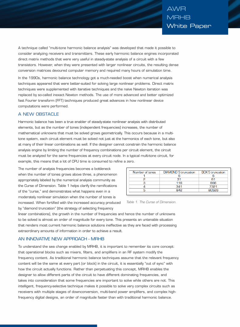
The number of analysis frequencies becomes a bottleneck
when the number of tones grows above three, a phenomenon
appropriately labeled by the numerical analysis community as
the curse of dimension. Table 1 helps clarify the ramifications
of the “curse,” and demonstrates what happens even in a
moderately nonlinear simulation when the number of tones is
increased. When fortified with the increased accuracy produced
by “diamond truncation” (the strategy of selecting frequency
linear combinations), the growth in the number of frequencies and hence the number of unknowns
to be solved is almost an order of magnitude for every tone. This presents an untenable situation
that renders most current harmonic balance solutions ineffective as they are faced with processing
extraordinary amounts of information in order to achieve a result.
An innovATive neW APPRoAch - MRhB
To understand the sea change enabled by MRhB, it is important to remember its core concept:
that operational blocks such as mixers, filters, and amplifiers in an Rf system modify the
frequency content. As traditional harmonic balance techniques assume that the relevant frequency
content will be the same at every part (or block) in the circuit, it is essentially “out of sync” with
how the circuit actually functions. Rather than perpetuating this concept, MRhB enables the
designer to allow different parts of the circuit to have different dominating frequencies, and
takes into consideration that some frequencies are important to solve while others are not. This
intelligent, frequency-selective technique makes it possible to solve very complex circuits such as
receivers with multiple stages of downconversion, multi-band power amplifiers, and complex high-
frequency digital designs, an order of magnitude faster than with traditional harmonic balance.
AWR MRHBWhite Paper
Table 1. The Curse of Dimension.
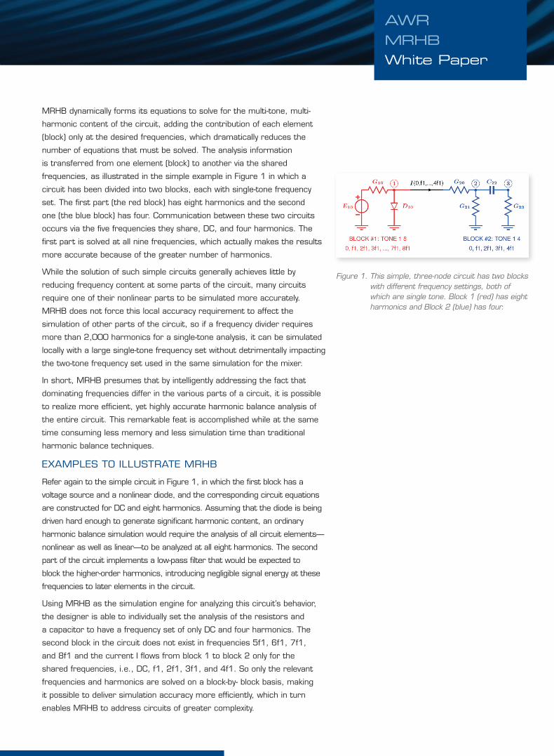
MRhB dynamically forms its equations to solve for the multi-tone, multi-
harmonic content of the circuit, adding the contribution of each element
(block) only at the desired frequencies, which dramatically reduces the
number of equations that must be solved. The analysis information
is transferred from one element (block) to another via the shared
frequencies, as illustrated in the simple example in figure 1 in which a
circuit has been divided into two blocks, each with single-tone frequency
set. The first part (the red block) has eight harmonics and the second
one (the blue block) has four. communication between these two circuits
occurs via the five frequencies they share, dc, and four harmonics. The
first part is solved at all nine frequencies, which actually makes the results
more accurate because of the greater number of harmonics.
While the solution of such simple circuits generally achieves little by
reducing frequency content at some parts of the circuit, many circuits
require one of their nonlinear parts to be simulated more accurately.
MRhB does not force this local accuracy requirement to affect the
simulation of other parts of the circuit, so if a frequency divider requires
more than 2,000 harmonics for a single-tone analysis, it can be simulated
locally with a large single-tone frequency set without detrimentally impacting
the two-tone frequency set used in the same simulation for the mixer.
in short, MRhB presumes that by intelligently addressing the fact that
dominating frequencies differ in the various parts of a circuit, it is possible
to realize more efficient, yet highly accurate harmonic balance analysis of
the entire circuit. This remarkable feat is accomplished while at the same
time consuming less memory and less simulation time than traditional
harmonic balance techniques.
exAMPles To illusTRATe MRhB
Refer again to the simple circuit in figure 1, in which the first block has a
voltage source and a nonlinear diode, and the corresponding circuit equations
are constructed for dc and eight harmonics. Assuming that the diode is being
driven hard enough to generate significant harmonic content, an ordinary
harmonic balance simulation would require the analysis of all circuit elements—
nonlinear as well as linear—to be analyzed at all eight harmonics. The second
part of the circuit implements a low-pass filter that would be expected to
block the higher-order harmonics, introducing negligible signal energy at these
frequencies to later elements in the circuit.
using MRhB as the simulation engine for analyzing this circuit’s behavior,
the designer is able to individually set the analysis of the resistors and
a capacitor to have a frequency set of only dc and four harmonics. The
second block in the circuit does not exist in frequencies 5f1, 6f1, 7f1,
and 8f1 and the current i flows from block 1 to block 2 only for the
shared frequencies, i.e., dc, f1, 2f1, 3f1, and 4f1. so only the relevant
frequencies and harmonics are solved on a block-by- block basis, making
it possible to deliver simulation accuracy more efficiently, which in turn
enables MRhB to address circuits of greater complexity.
AWR MRHBWhite Paper
Figure 1. This simple, three-node circuit has two blocks with different frequency settings, both of which are single tone. Block 1 (red) has eight harmonics and Block 2 (blue) has four.
looking at the two relevant domains in which MRhB can be employed:
• in the single-tone, multiple-frequency domain of figure 1, MRhB
selects only the required nonlinear elements rather than all nonlinear
harmonics propagated to all circuit elements
• in the multi-tone, multiple-frequency domain of figure 2, MRhB
reduces the overall tone-frequency solution space yet maintains high
accuracy through the use of hybrid-tones
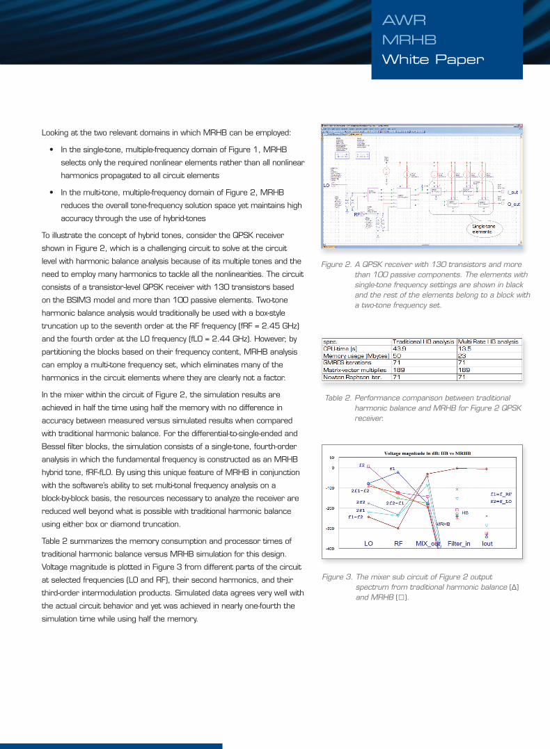
To illustrate the concept of hybrid tones, consider the QPsK receiver
shown in figure 2, which is a challenging circuit to solve at the circuit
level with harmonic balance analysis because of its multiple tones and the
need to employ many harmonics to tackle all the nonlinearities. The circuit
consists of a transistor-level QPsK receiver with 130 transistors based
on the BsiM3 model and more than 100 passive elements. Two-tone
harmonic balance analysis would traditionally be used with a box-style
truncation up to the seventh order at the Rf frequency (fRf = 2.45 ghz)
and the fourth order at the lo frequency (flo = 2.44 ghz). however, by
partitioning the blocks based on their frequency content, MRhB analysis
can employ a multi-tone frequency set, which eliminates many of the
harmonics in the circuit elements where they are clearly not a factor.
in the mixer within the circuit of figure 2, the simulation results are
achieved in half the time using half the memory with no difference in
accuracy between measured versus simulated results when compared
with traditional harmonic balance. for the differential-to-single-ended and
Bessel filter blocks, the simulation consists of a single-tone, fourth-order
analysis in which the fundamental frequency is constructed as an MRhB
hybrid tone, fRf-flo. By using this unique feature of MRhB in conjunction
with the software’s ability to set multi-tonal frequency analysis on a
block-by-block basis, the resources necessary to analyze the receiver are
reduced well beyond what is possible with traditional harmonic balance
using either box or diamond truncation.
Table 2 summarizes the memory consumption and processor times of
traditional harmonic balance versus MRhB simulation for this design.
voltage magnitude is plotted in figure 3 from different parts of the circuit
at selected frequencies (lo and Rf), their second harmonics, and their
third-order intermodulation products. simulated data agrees very well with
the actual circuit behavior and yet was achieved in nearly one-fourth the
simulation time while using half the memory.
AWR MRHBWhite Paper
Figure 2. A QPSK receiver with 130 transistors and more than 100 passive components. The elements with single-tone frequency settings are shown in black and the rest of the elements belong to a block with a two-tone frequency set.
Figure 3. The mixer sub circuit of Figure 2 output spectrum from traditional harmonic balance (Δ) and MRHB (□).
Table 2. Performance comparison between traditional harmonic balance and MRHB for Figure 2 QPSK receiver.
exAMPle: MRhB succeeds WheRe hB fAils
More than just speeding up traditional hB, with MRhB it is possible
to simulate circuits that are impossible for harmonic balance to tackle
due to the memory limitations of its formulation. A key feature of the
MRhB technique is that the hB solution space can be defined on a
block-by-block basis and, as such, limits the harmonics over which the
simulator must solve. in other words, MRhB redefines the tones so
as to advantageously direct the simulator to solve for only those tones
that matter.
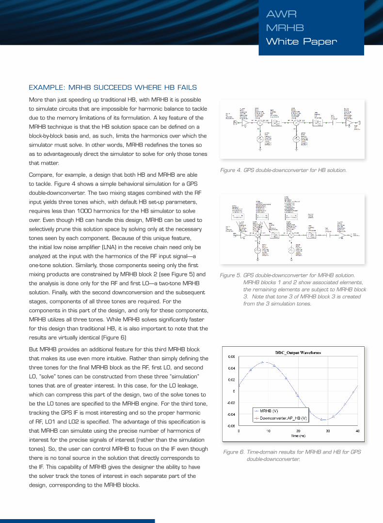
compare, for example, a design that both hB and MRhB are able
to tackle. figure 4 shows a simple behavioral simulation for a gPs
double-downconverter. The two mixing stages combined with the Rf
input yields three tones which, with default hB set-up parameters,
requires less than 1000 harmonics for the hB simulator to solve
over. even though hB can handle this design, MRhB can be used to
selectively prune this solution space by solving only at the necessary
tones seen by each component. Because of this unique feature,
the initial low noise amplifier (lnA) in the receive chain need only be
analyzed at the input with the harmonics of the Rf input signal—a
one-tone solution. similarly, those components seeing only the first
mixing products are constrained by MRhB block 2 (see figure 5) and
the analysis is done only for the Rf and first lo—a two-tone MRhB
solution. finally, with the second downconversion and the subsequent
stages, components of all three tones are required. for the
components in this part of the design, and only for these components,
MRhB utilizes all three tones. While MRhB solves significantly faster
for this design than traditional hB, it is also important to note that the
results are virtually identical (figure 6)
But MRhB provides an additional feature for this third MRhB block
that makes its use even more intuitive. Rather than simply defining the
three tones for the final MRhB block as the Rf, first lo, and second
lo, “solve” tones can be constructed from these three “simulation”
tones that are of greater interest. in this case, for the lo leakage,
which can compress this part of the design, two of the solve tones to
be the lo tones are specified to the MRhB engine. for the third tone,
tracking the gPs if is most interesting and so the proper harmonic
of Rf, lo1 and lo2 is specified. The advantage of this specification is
that MRhB can simulate using the precise number of harmonics of
interest for the precise signals of interest (rather than the simulation
tones). so, the user can control MRhB to focus on the if even though
there is no tonal source in the solution that directly corresponds to
the if. This capability of MRhB gives the designer the ability to have
the solver track the tones of interest in each separate part of the
design, corresponding to the MRhB blocks.
Figure 6. Time-domain results for MRHB and HB for GPS double-downconverter.
AWR MRHBWhite Paper
Figure 5. GPS double-downconverter for MRHB solution. MRHB blocks 1 and 2 show associated elements, the remaining elements are subject to MRHB block 3. Note that tone 3 of MRHB block 3 is created from the 3 simulation tones.
Figure 4. GPS double-downconverter for HB solution.
AWR.Tv™
AWR, 1960 east grand Avenue, suite 430, el segundo, cA 90245, usATel: +1 (310) 726-3000 fax: +1 (310) 726-3005 www.awrcorp.com
copyright © 2010 AWR corporation. All rights reserved. AWR, the AWR logo, APlAc and Microwave office are registered trademarks and MRhB and AWR.Tv are trademarks of AWR corporation.
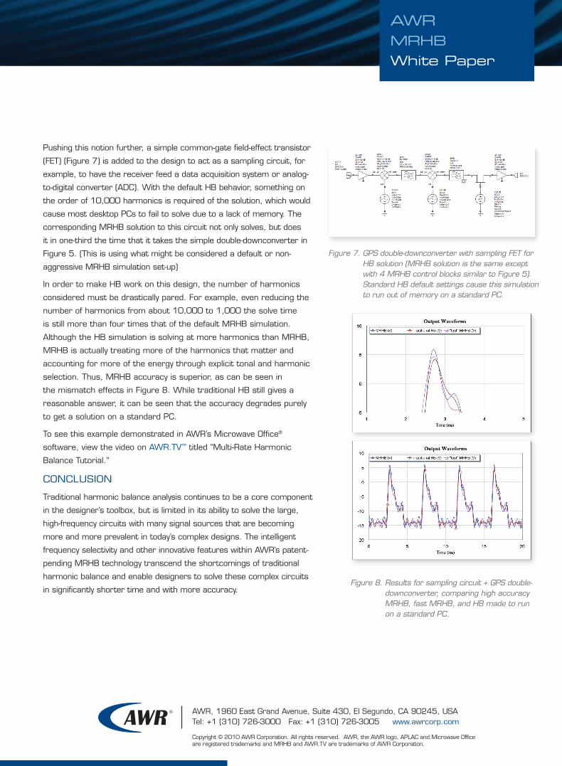
Pushing this notion further, a simple common-gate field-effect transistor
(feT) (figure 7) is added to the design to act as a sampling circuit, for
example, to have the receiver feed a data acquisition system or analog-
to-digital converter (Adc). With the default hB behavior, something on
the order of 10,000 harmonics is required of the solution, which would
cause most desktop Pcs to fail to solve due to a lack of memory. The
corresponding MRhB solution to this circuit not only solves, but does
it in one-third the time that it takes the simple double-downconverter in
figure 5. (This is using what might be considered a default or non-
aggressive MRhB simulation set-up)
in order to make hB work on this design, the number of harmonics
considered must be drastically pared. for example, even reducing the
number of harmonics from about 10,000 to 1,000 the solve time
is still more than four times that of the default MRhB simulation.
Although the hB simulation is solving at more harmonics than MRhB,
MRhB is actually treating more of the harmonics that matter and
accounting for more of the energy through explicit tonal and harmonic
selection. Thus, MRhB accuracy is superior, as can be seen in
the mismatch effects in figure 8. While traditional hB still gives a
reasonable answer, it can be seen that the accuracy degrades purely
to get a solution on a standard Pc.
To see this example demonstrated in AWR’s Microwave office®
software, view the video on AWR.Tv™ titled “Multi-Rate harmonic
Balance Tutorial.”
conclusion
Traditional harmonic balance analysis continues to be a core component
in the designer’s toolbox, but is limited in its ability to solve the large,
high-frequency circuits with many signal sources that are becoming
more and more prevalent in today’s complex designs. The intelligent
frequency selectivity and other innovative features within AWR’s patent-
pending MRhB technology transcend the shortcomings of traditional
harmonic balance and enable designers to solve these complex circuits
in significantly shorter time and with more accuracy.
AWR MRHBWhite Paper
Figure 7. GPS double-downconverter with sampling FET for HB solution (MRHB solution is the same except with 4 MRHB control blocks similar to Figure 5). Standard HB default settings cause this simulation to run out of memory on a standard PC.
Figure 8. Results for sampling circuit + GPS double-downconverter, comparing high accuracy MRHB, fast MRHB, and HB made to run on a standard PC.


