FINAL REPORT 2013 UPPER GREEN RIVER
WINTER OZONE STUDY
Prepared for:
Ms. Cara Keslar Wyoming DEQ – Air Quality Division
Herschler Building 122 West 25th Street
Cheyenne, Wyoming 82002
By the TEAM of:
Meteorological Solutions Inc. T & B Systems
August 2013

UGWOS 2013 MSI i
FINAL REPORT 2013 UPPER GREEN RIVER WINTER OZONE STUDY
TABLE OF CONTENTS Section Page 1.0 INTRODUCTION ........................................................................................................... 1-1 2.0 SUMMARY OF FIELD OPERATIONS......................................................................... 2-1
2.1 Overview .............................................................................................................. 2-1
2.1.1 Planning Process ...................................................................................... 2-1 2.1.2 Monitoring Sites....................................................................................... 2-2 2.1.3 UGWOS Website ..................................................................................... 2-5
2.2 Field Measurements ........................................................................................... 2-11 2.2.1 WDEQ Long-Term Monitoring Sites .................................................... 2-12 2.2.2 True NO2 Measurements ........................................................................ 2-15 2.2.3 Mobile Trailer Measurements: Big Piney and Jonah Field ................... 2-16 2.2.4 Mesonet Monitoring Stations ................................................................. 2-19 2.2.5 VOC Canister Sampling ........................................................................ 2-22 2.2.6 miniSODAR™ ....................................................................................... 2-23 2.2.7 Ozonesondes/Radiosondes ..................................................................... 2-24
2.3 Designated VOC Canister Sampling Days ........................................................ 2-24 2.3.1 Forecasts for IOP/VOC Canister Sampling Events ............................... 2-25 2.3.2 Synoptic Weather Summaries of Canister Sampling Events ................. 2-27
3.0 DATA QUALITY ASSURANCE, VALIDATION AND ARCHIVING ..................... 3-1
3.1 Database Management ......................................................................................... 3-1 3.2 Quality Assurance Program ................................................................................. 3-3
3.2.1 Calibrations .............................................................................................. 3-8 3.2.2 Quality Assurance Audits ........................................................................ 3-9 3.2.2.1 Performance Audits ..................................................................... 3-9 3.2.2.2 System Audits ............................................................................ 3-12 3.2.2.3 Processing of the miniSODAR™ data ...................................... 3-15
3.3 Data Archiving ................................................................................................... 3-15
4.0 DATA ANALYSIS .......................................................................................................... 4-1
4.1 Summary of 2013 Meteorological and Air Quality Conditions and Comparison with Prior Years ................................................................................................... 4-1
4.1.1 700 mb Comparison 2013 versus 2007-2012 .......................................... 4-1 4.1.2 UGWOS Snow Cover in 2012 and 2013 ................................................. 4-4

UGWOS 2013 MSI ii
Table of Contents Continued
Section Page 4.2 Ozone Spatial and Temporal Distribution ........................................................... 4-6
4.2.1 Discussion of Spatial and Temporal Distribution of O3 during Designated VOC Canister Sampling Periods ........................................................... 4-11 4.2.2 Surface Wind Patterns Affiliated with Elevated Ozone during Designated VOC Sampling Periods .......................................................................... 4-15 4.2.3 Comparison of Ozone in 2013 with 2005-2012 ..................................... 4-18 4.2.4 Comparison of NOx and PM during UGWOS 2013 with 2006-2012 ... 4-20 4.2.5 Comparison of NMHC and THC during UGWOS 2013 with 2010-2012 .............................................................................................. 4-23
4.3 VOC Canister Sampling .................................................................................... 4-26 4.3.1 Jonah and Jonah 2 .................................................................................. 4-32 4.3.2 Comparison of 2013 to 2012 Study ....................................................... 4-34 4.3.3 VOC Maximum Incremental Reactivity Analysis ................................. 4-36 4.3.3 VOC Quality Control Results ................................................................ 4-38
4.4 miniSODAR™ Data .......................................................................................... 4-41 4.5 Ozonesondes/Radiosondes ................................................................................. 4-45
5.0 SUMMARY, CONCLUSIONS, AND RECOMMENDATIONS................................... 5-1
5.1 Summary .............................................................................................................. 5-1 5.1.1 UGWOS 2013 Field Operations .............................................................. 5-2
5.2 Conclusions/Observations.................................................................................... 5-3 5.3 Recommendations ................................................................................................ 5-5
5.3.1 WDEQ Upper Air Sounding System ....................................................... 5-5 5.3.2 Tall Tower Measurements ....................................................................... 5-6 5.3.3 Expansion of Surface-Based Monitoring Network during UGWOS Using WDEQ-Owned Mesonet/VOC Canister Sampling Equipment ... 5-7 5.3.4 Lidar and Radiometer Measurements using the San Jose State Fire Research Lab ............................................................................................ 5-7 5.3.5 Ceilometer ................................................................................................ 5-9 5.3.6 Unmanned Aircraft .................................................................................. 5-9 5.3.7 Nocturnal Transport of NOx along Drainage Basins ............................. 5-11 5.3.8 Improved miniSodar Data Assimilation and Analysis ........................... 5-13
6.0 ACKNOWLEDGEMENTS 2013 .................................................................................... 6-1 7.0 REFERENCES ................................................................................................................ 7-1 Table 2-1 Summary of Measurement Methods Used During UGWOS 2013 .................................. 2-4
UGWOS 2013 MSI iii
Table of Contents Continued
Table Page 3-1 Data Quality Control Codes Used in UGWOS Database ................................................ 3-2 3-2 Method TO-14 DHA Compound List .............................................................................. 3-5 3-3 Summary of QC Criteria for TO-14 Modified for DHA and PAMS Hydrocarbon Analysis............................................................................................................................ 3-8 3-4 Mesonet Ozone Audit Results ....................................................................................... 3-11 3-5 Jonah Air Quality Audit Result Summary ..................................................................... 3-11 4-1 Intensive Operational Periods by Year ............................................................................ 4-3 4-2 Maximum Eight-Hour Average Ozone Concentrations (ppb) for Boulder (BD), Daniel (DN), Jonah, Juel Springs, Mesa, Pinedale (PD), Warbonnet (WB), Wyoming
Range (WR), and Big Piney (BP) on Days When at Least One Site Recorded Concentrations >55 ppb ................................................................................................. 4-11 4-3 Eight-Hour Monthly Average and Maximum Ozone by Year for Jonah, Boulder, Daniel,
Pinedale, Juel Springs, and Wyoming Range ................................................................ 4-19 4-4 Monthly Average One-Hour NO and NO2 Concentrations by Year for Jonah, Boulder,
Daniel, Pinedale, Juel Springs, and Wyoming Range ................................................... 4-21 4-5 Monthly Average PM10 and PM2.5 Concentrations by Year for Boulder, Daniel, Pinedale, and Wyoming Range ...................................................................................... 4-22 4-6 Monthly Average CH4, NMHC, and THC Concentrations by Year for Boulder and Big Piney ........................................................................................................................ 4-23 4-7 Number of Days That Highest 1-Hr NMHC Concentration Exceeded 2.0 ppm and 4.0 ppm at Boulder and Bug Piney ................................................................................ 4-24 4-8 Wind Speed Statistics for VOC Sample Locations ........................................................ 4-31 4-9 Top Compounds by Concentration and Potential Reactivity ......................................... 4-38 4-9 VOC Quality Control Results ........................................................................................ 4-38 4-10 Boulder Mixing Height and Meteorological Metrics – January 15 through February 28.................................................................................................................................... 4-42 Figure 2.1 Active Monitoring Stations in the UGWOS 2013 Study Domain ................................... 2-3 2.2 Current Ozone Concentrations with Website Menu ........................................................ 2-6 2.3 Single Station Strip Charts Example................................................................................ 2-7 2.4 Ozone Strip Charts from All Sites for a User-Selected Time Period .............................. 2-8 2.5 VOC Canister Sample Composition for Each Sampling Site .......................................... 2-8 2.6 Project Weather/Ozone Outlook Example ....................................................................... 2-9 2.7 Example of a Radiosonde Balloon Flight Plot from January 17, 2013 ........................... 2-9 2.8 Images from Mesonet Site Cameras Updated on the Website Every 15 Minutes ......... 2-10 2.9 Current Equipment Status .............................................................................................. 2-10 2.10 UGWOS 2013 Monitoring Site Data Retrieval Status .................................................. 2-11 2.11 Photograph of Pinedale Monitoring Station .................................................................. 2-13 2.12 Boulder Monitoring Site during UGWOS 2013 ............................................................ 2-14
UGWOS 2013 MSI iv
Table of Contents Continued
Figure Page 2.13 Boulder Meteorological Station with TUVR Sensors and UGWOS VOC Sampling
Tripod ............................................................................................................................. 2-14 2.14 Photograph of Interior of Boulder Monitoring Station .................................................. 2-15 2.15 Mobile Trailer and VOC Sampling Tripod at the Big Piney Site .................................. 2-17 2.16 Jonah Field Monitoring Site with Adjacent VOC Tripod .............................................. 2-18 2.17 Jonah 2 VOC Monitoring Site ....................................................................................... 2-19 2.18 Mesa Mesonet Site ......................................................................................................... 2-20 2.19 Warbonnet Mesonet Site ................................................................................................ 2-21 2.20 Paradise Mesonet Site .................................................................................................... 2-21 2.21 miniSODAR™ ............................................................................................................... 2-23 2.22 Example Weather Outlook ............................................................................................. 2-26 2.23 700 mb Level Chart at 0500 MST January 20, 2013 ..................................................... 2-28 2.24 Surface Chart at 0500 MST January 20, 2013 ............................................................... 2-28 2.25 700 mb Level Chart at 0500 MST February 3, 2013 ..................................................... 2-29 2.26 Surface Chart at 0500 MST February 3, 2013 ............................................................... 2-30 2.27 700 mb Chart at 0500 MST March 14, 2013 ................................................................. 2-31 2.28 Surface Chart at 0500 MST March 14, 2013 ................................................................. 2-32 2.29 700 mb Chart at 0500 MST March 28, 2013 ................................................................. 2-33 2.30 Surface Chart at 0500 MST March 28, 2013 ................................................................. 2-33 4.1 700 mb Averages for 2007-2013 ..................................................................................... 4-2 4.2 Boulder Site January 15, 2012 (left) and 2013 (right) ..................................................... 4-5 4.3 Boulder Site March 2, 2012 (left) and 2013 (right) ......................................................... 4-6 4.4 Estimated Snow Depth at Boulder Based on Snow Stick Images ................................... 4-6 4.5 Maximum Eight-Hour and One-Hour Average Ozone Concentrations in the UGRB during UGWOS 2013 ...................................................................................................... 4-7 4.6 Running Eight-Hour Ozone Concentrations during UGWOS 2013 ................................ 4-8 4.7 Daily Maximum Eight-Hour Ozone Concentrations, UGWOS 2013 ........................... 4-10 4.8 One-Hour Average Ozone during Designated VOC Sampling Period 1 ....................... 4-13 4.9 One-Hour Average Ozone during Designated VOC Sampling Period 2 ....................... 4-13 4.10 One-Hour Average Ozone during Designated VOC Sampling Period 3 ....................... 4-14 4.11 One-Hour Average Ozone during Designated VOC Sampling Period 4 ....................... 4-15 4.12 One-Hour Average Ozone and Wind at Paradise and Juel Springs during VOC Sampling Period 1 .......................................................................................................................... 4-16 4.13 One-Hour Average Ozone and Wind at Paradise and Juel Springs during VOC Sampling Period 2 .......................................................................................................................... 4-17 4.14 Comparison of Maximum 8-Hour Ozone and Daily Average NMHC at Boulder for UGWOS 2011-2013. Linear regression fit for 2013 data is shown ............................... 4-24 4.15 Comparison of Maximum 8-Hour Ozone and Daily Average NMHC at Big Piney for UGWOS 2012-2013. Linear regression fit for 2013 data is shown ............................... 4-25 4.16 VOC Concentrations from Canisters Collected at Boulder, Juel Springs, Jonah, and Jonah 2 ........................................................................................................................... 4-27

UGWOS 2013 MSI v
Table of Contents Continued
Figure Page 4.17 VOC Concentrations from Canisters Collected at Paradise, Warbonnet, Mesa, and Big Piney ........................................................................................................................ 4-28 4.18 Relative Composition from Canisters Collected at Boulder, Juel Springs, Jonah, and Jonah 2 ........................................................................................................................... 4-29 4.19 Relative Composition from Canisters Collected at Paradise, Warbonnet, Mesa, and Big Piney ........................................................................................................................ 4-30 4.20 Total NMHC and Sample Time Windroses for Jonah and Jonah 2 ............................... 4-33 4.21 Boulder VOC Data From UGWOS 2012 and 2013....................................................... 4-35 4.22 Percent Composition of VOC Classifications................................................................ 4-36 4.23 Actual and MIR Enhanced Total NMHC ...................................................................... 4-37 4.24 February 3, 2013 Collocated Sample Comparison from Juel Springs ........................... 4-39 4.25 March 14, 2013 Collocated Sample Comparison from Warbonnet ............................... 4-39 4.26 March 28, 2013 Collocated Sample Comparison from Big Piney ................................. 4-40 4.27 January 19, 2013 Unintentional Collocated Sample Comparison from Boulder ........... 4-41 4.28 Radiosonde Balloon Launch on January 17, 2013 Test Day ......................................... 4-45 4.29 Morning Radiosonde on January 17, 2013 Test Day ..................................................... 4-46 4.30 Afternoon Ozonesonde/Radiosonde on January 17, 2013 Test Day ............................. 4-46 Appendix A Monitoring and Quality Assurance Plan B Microsoft Access Database Description

UGWOS 2013 1-1 MSI
1.0 INTRODUCTION
The Wyoming Department of Environmental Quality – Air Quality Division (AQD)
sponsored the Upper Green Winter Ozone Study (UGWOS) during the period January 15 to
March 31, 2013. This research program has been conducted each year since 2007 to investigate
wintertime ozone formation in the Upper Green River Basin (UGRB) leading to concentrations
of ambient ozone (O3) exceeding the National Ambient Air Quality Standard (NAAQS) which is
currently set at a daily maximum eight-hour average of 75 parts per billion (ppb). During each
year’s field effort, data were collected from a network of long-term air quality monitoring
stations, temporary monitoring stations, upper air data from soundings and/or miniSODAR™,
and various specialized ozone precursor measurement systems. Quality assurance project plans,
data, and reports from previous UGWOS field efforts (2007-2012) are posted on the Monitoring
Information Page of the WDEQ-AQD website.1
In 2013, AQD contracted with Meteorological Solutions Inc. (MSI) and sub-contractor
T & B Systems to conduct a field measurement program which emphasized the spatial
distribution of ozone and ozone precursors. MSI was responsible for overall project
management, station siting, ozone event forecasting, project website hosting, project database,
data collection and management, data validation and reporting as well as field monitoring
operations. Field operations included the following:
An air quality technician stationed full-time in the project area for the duration of the
UGWOS field effort to install and operate eight (8) canister sampling sites, perform
routine quality control checks on air quality sites, and provide immediate
troubleshooting and repair for UGWOS and existing long-term monitoring sites in the
project domain;
Installation, calibration and operation of three mesonet sites providing continuous
ozone, wind speed and direction, temperature and camera images;
1 http://deq.state.wy.us/aqd/Monitoring%20Data.asp

UGWOS 2013 1-2 MSI
Installation, calibration, and operation of a temporary ambient air monitoring station
in the Jonah Field which provided continuous measurements of O3 and oxides of
nitrogen (NOx) as well as wind speed, wind direction, temperature and camera
images;
Speciated hydrocarbon sampling using stainless steel canisters at eight (8) sites on
designated sampling days; and
Ozonesonde/radiosonde operations (2 flights per day) during periods when conditions
favoring potential elevated ozone episodes were forecast.
T & B Systems provided independent quality assurance audits, an updated Quality
Assurance Project Plan (QAPP) and data collection and validation and analysis for AQD’s
miniSODARTM which continued to operate at the Boulder monitoring site.
Field operations for UGWOS 2013 started on January 15, 2013 and continued through
March 31, 2013. Daily weather outlooks were issued by MSI’s forecast meteorologist in order to
identify periods when ambient ozone concentrations in the UGRB were likely to be elevated and
to provide an alert to field personnel so additional speciated VOC canister and upper air
ozonesonde/radiosonde measurements could be implemented during these Intensive Operational
Periods (IOP’s). IOP conditions never materialized during the UGWOS 2013 field measurement
season and instead there were five designated volatile organic compound (VOC) sampling days
which were forecast to be characterized by high pressure, light winds and sunny skies.
This report presents a summary of UGWOS 2013 field operations, quality assurance
activities, and the results of the field measurement program. Section 2.0 presents an overview of
field measurement operations including the ozone and ozone precursor measurements and
provides synoptic weather summaries for the designated VOC sampling days. Section 3.0
describes database management, quality assurance, data validation, and data archiving.
Monitoring results are described in Section 4.0. Section 5.0 presents a summary of the findings,
conclusions based on the findings, and recommendations. UGWOS 2013 measurement data are
available in an ACCESS database on the AQD website.
USWOS 2013 2-1 MSI
2.0 SUMMARY OF FIELD OPERATIONS
This section provides a description of measurement platforms active during UGWOS
2013, operational forecasts, and synoptic weather summaries during 2013 designated VOC
sampling periods.
2.1 Overview
UGWOS 2013 field operations were scheduled for January 15, 2013 through March 31,
2013. All UGWOS 2013 monitoring sites were installed, calibrated, and ready for operations by
January 14, 2013. Forecasting for elevated ozone conditions started on January 15, 2013 and
continued through March 31, 2013.
2.1.1 Planning Process
A siting trip was conducted with AQD personnel on December 12, 2012 to locate a
suitable replacement for the former Jonah site to monitor ambient conditions in the Jonah Field
area. After investigating several possible alternatives, a site just outside the property line of the
Linn Energy facility was selected as the best alternative since the facility was willing to allow
access to their power. This monitoring location is approximately six kilometers west of the 2012
site and representative of the Jonah Field.
During UGWOS 2013, three (3) tripod-mounted solar-powered mesonet sites were
operated at locations utilized during previous measurement programs. These included two
former mesonet sites – Mesa and Warbonnet, and the 2011 location of tethered balloon
measurements now designated as the Paradise site.

USWOS 2013 2-2 MSI
These sites, as well as an additional control site for VOC canister measurements
conducted at the new location of the Jonah site mentioned above, required clearance for wildlife
concerns and Bureau of Land Management (BLM) approval. BLM approval for the three
mesonet sites was granted on January 7, 2013 and on January 22, 2013 for the additional Jonah
VOC control site designated as Jonah 2.
As in 2012, AQD-owned VOC sampling systems were utilized for the UGWOS 2013
VOC sampling effort. Sampling systems were retrieved in December, 2012, cleaned, leak-
checked and tested for contamination prior to operational use during UGWOS 2013.
2.1.2 Monitoring Sites
All of the currently operating long-term WDEQ-AQD monitoring stations in the UGRB,
three mesonet sites, the WDEQ miniSODAR, mobile trailers at Big Piney and in the Jonah field,
and a VOC measurement control site for the Jonah field station provided meteorological and air
quality data for the UGWOS 2013 database. A map showing the measurement stations active
during the UGWOS 2013 program is shown in Figure 2.1.
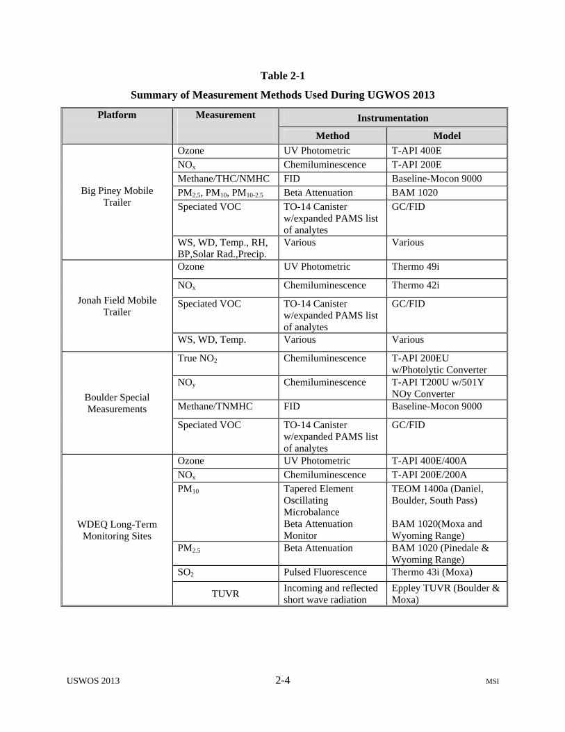
A summary of the instrumentation and parameters measured at each sampling platform is
presented in Table 2-1.

USWOS 2013 2-3 MSI
Figure 2.1 Active Monitoring Stations in the UGWOS 2013 Study Domain
USWOS 2013 2-4 MSI
Table 2-1
Summary of Measurement Methods Used During UGWOS 2013
Platform
Measurement
Instrumentation
Method Model
Big Piney Mobile Trailer
Ozone UV Photometric T-API 400E NOx Chemiluminescence T-API 200E Methane/THC/NMHC FID Baseline-Mocon 9000 PM2.5, PM10, PM10-2.5 Beta Attenuation BAM 1020 Speciated VOC TO-14 Canister
w/expanded PAMS list of analytes
GC/FID
WS, WD, Temp., RH, BP,Solar Rad.,Precip.
Various Various
Jonah Field Mobile Trailer
Ozone UV Photometric Thermo 49i
NOx Chemiluminescence Thermo 42i
Speciated VOC TO-14 Canister w/expanded PAMS list of analytes
GC/FID
WS, WD, Temp. Various Various
Boulder Special Measurements
True NO2 Chemiluminescence T-API 200EU w/Photolytic Converter
NOy Chemiluminescence T-API T200U w/501Y NOy Converter
Methane/TNMHC FID Baseline-Mocon 9000
Speciated VOC TO-14 Canister w/expanded PAMS list of analytes
GC/FID
WDEQ Long-Term Monitoring Sites
Ozone UV Photometric T-API 400E/400A NOx Chemiluminescence T-API 200E/200A PM10 Tapered Element
Oscillating Microbalance Beta Attenuation Monitor
TEOM 1400a (Daniel, Boulder, South Pass) BAM 1020(Moxa and Wyoming Range)
PM2.5 Beta Attenuation BAM 1020 (Pinedale & Wyoming Range)
SO2 Pulsed Fluorescence Thermo 43i (Moxa)
TUVR Incoming and reflected short wave radiation
Eppley TUVR (Boulder & Moxa)
USWOS 2013 2-5 MSI
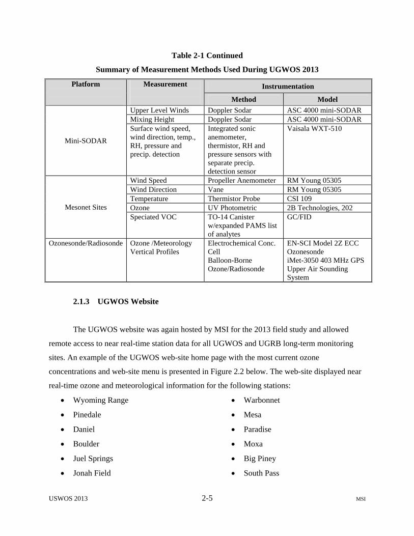
Table 2-1 Continued
Summary of Measurement Methods Used During UGWOS 2013
Platform
Measurement
Instrumentation
Method Model
Mini-SODAR
Upper Level Winds Doppler Sodar ASC 4000 mini-SODAR Mixing Height Doppler Sodar ASC 4000 mini-SODAR Surface wind speed, wind direction, temp., RH, pressure and precip. detection
Integrated sonic anemometer, thermistor, RH and pressure sensors with separate precip. detection sensor
Vaisala WXT-510
Mesonet Sites
Wind Speed Propeller Anemometer RM Young 05305 Wind Direction Vane RM Young 05305 Temperature Thermistor Probe CSI 109 Ozone UV Photometric 2B Technologies, 202 Speciated VOC TO-14 Canister
w/expanded PAMS list of analytes
GC/FID
Ozonesonde/Radiosonde Ozone /Meteorology Vertical Profiles
Electrochemical Conc. Cell Balloon-Borne Ozone/Radiosonde
EN-SCI Model 2Z ECC Ozonesonde iMet-3050 403 MHz GPS Upper Air Sounding System
2.1.3 UGWOS Website
The UGWOS website was again hosted by MSI for the 2013 field study and allowed
remote access to near real-time station data for all UGWOS and UGRB long-term monitoring
sites. An example of the UGWOS web-site home page with the most current ozone
concentrations and web-site menu is presented in Figure 2.2 below. The web-site displayed near
real-time ozone and meteorological information for the following stations:
Wyoming Range
Pinedale
Daniel
Boulder
Juel Springs
Jonah Field
Warbonnet
Mesa
Paradise
Moxa
Big Piney
South Pass

USWOS 2013 2-6 MSI
Figure 2.2 Current Ozone Concentrations with Website Menu

USWOS 2013 2-7 MSI
In addition to continually updated ozone information, wind speed, wind direction, and
temperature data were displayed on similar pages. Data were plotted on a project base map and
updated as often as every five minutes. Recent air quality and meteorological data were also
presented as a single station display in strip chart format. (See Figure 2.3) Ozone or
meteorological parameters from all sites were displayed simultaneously on an individual page for
a user-selected time period (Figure 2.4). VOC canister sample data were available as bar graphs
for each site’s samples showing sample composition as ppbC for the following groupings:
oxygenates, olefins, napthlenes, aromatics, isoparaffins, and paraffins (Figure 2.5). The project
weather and ozone outlook page was updated on a daily basis (Figure 2.6).
Ozonesonde/radiosonde sounding plots were posted on the web page soon after sounding runs
were completed (Figure 2.7). Camera images from mesonet (Figure 2.8) and long-term
monitoring sites were posted on the website and updated as often as every 15 minutes. A site
equipment matrix provided information which was updated whenever equipment status changed
(Figure 2.9). A monitoring site data retrieval status table (Figure 2.10) was updated continually
on the website showing the latest time/date when data were retrieved from each site. The project
website also provided links to the Wyvisnet, the miniSODAR data, and the WYDOT Farson
camera.
Figure 2.3 Single Station Strip Charts Example

USWOS 2013 2-8 MSI
Figure 2.4 Ozone Strip Charts from All Sites for a User-Selected Time Period
Figure 2.5 VOC Canister Sample Composition for Each Sampling Site
USWOS 2013 2-9 MSI
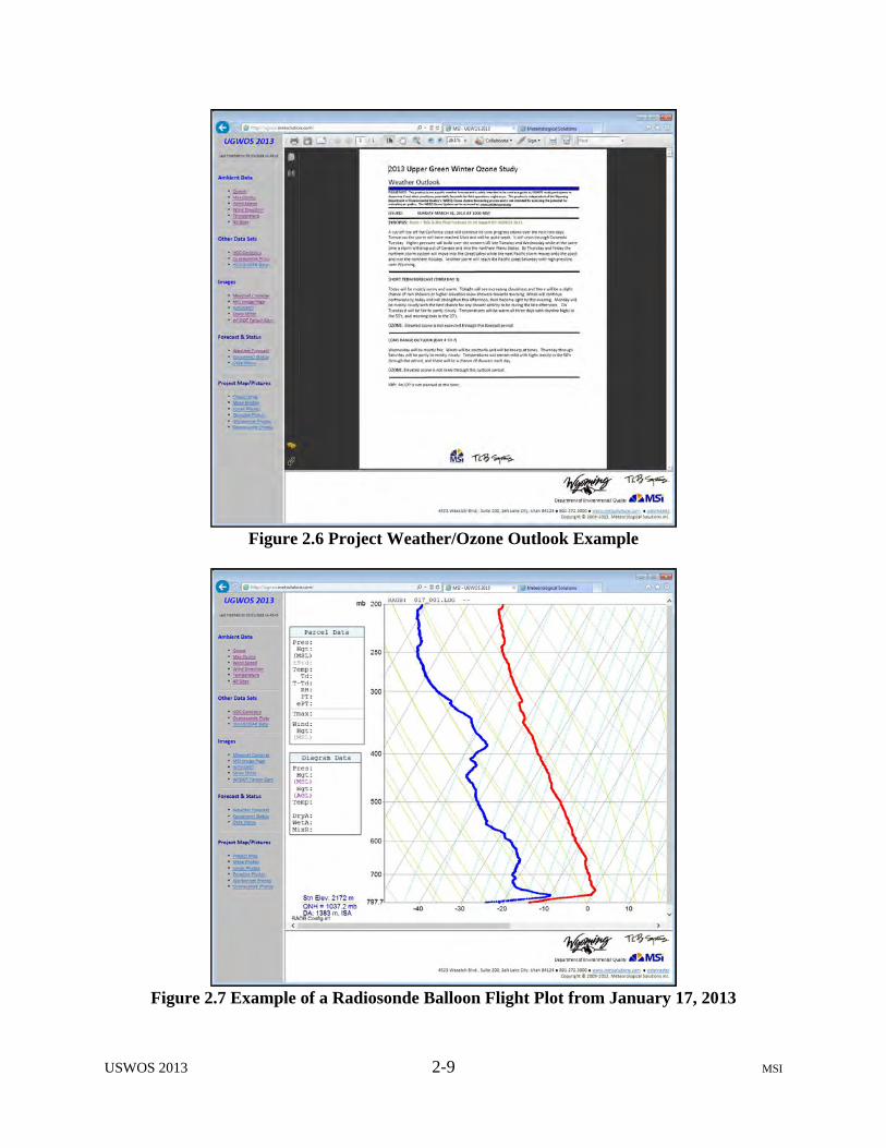
Figure 2.6 Project Weather/Ozone Outlook Example
Figure 2.7 Example of a Radiosonde Balloon Flight Plot from January 17, 2013

USWOS 2013 2-10 MSI
Figure 2.8 Images from Mesonet Site Cameras Updated on the Website Every 15 Minutes
Figure 2.9 Current Equipment Status

USWOS 2013 2-11 MSI
Figure 2.10 UGWOS 2013 Monitoring Site Data Retrieval Status
2.2 Field Measurements
Measurement stations which provided data for the UGWOS 2013 database included the
long-term WDEQ-AQD monitoring stations operating in the UGRB study area, two WDEQ
mobile trailer monitoring sites at Big Piney and the Jonah Field, and the WDEQ mini-SODAR
located adjacent to the Boulder monitoring station. Three mesonet sites collected ozone,
meteorological data and camera images on solar-powered tripods during UGWOS 2013. During
the field measurement season, VOC canister samples were collected on designated days at eight
locations - the two mobile trailer sites, the three mesonet sites, the Jonah 2 site and two of the
long-term monitoring stations – Boulder and Juel Springs. The Ozone/Radiosonde tracking
system was set up and operated at the Boulder monitoring site.
USWOS 2013 2-12 MSI
2.2.1 WDEQ Long-Term Monitoring Sites
WDEQ monitoring stations in the UGRB which were actively collecting data during
UGWOS 2013 included Wyoming Range, Daniel South, Boulder, Pinedale, Juel Springs, South
Pass, and Moxa. Long-term monitoring sites transmit camera images taken from the site every
15 minutes. These sites also typically measure wind speed and direction at 10 meters,
temperature, relative humidity, barometric pressure, solar radiation and precipitation. Boulder
and Moxa were also equipped to measure total UV radiation including incoming and reflected
short wave radiation in the 295-385 nm range. Air quality parameters measured at the long-term
sites included ozone, oxides of nitrogen, and particulate matter. The Boulder monitoring site
included additional enhanced measurements described below. The Moxa site also measures
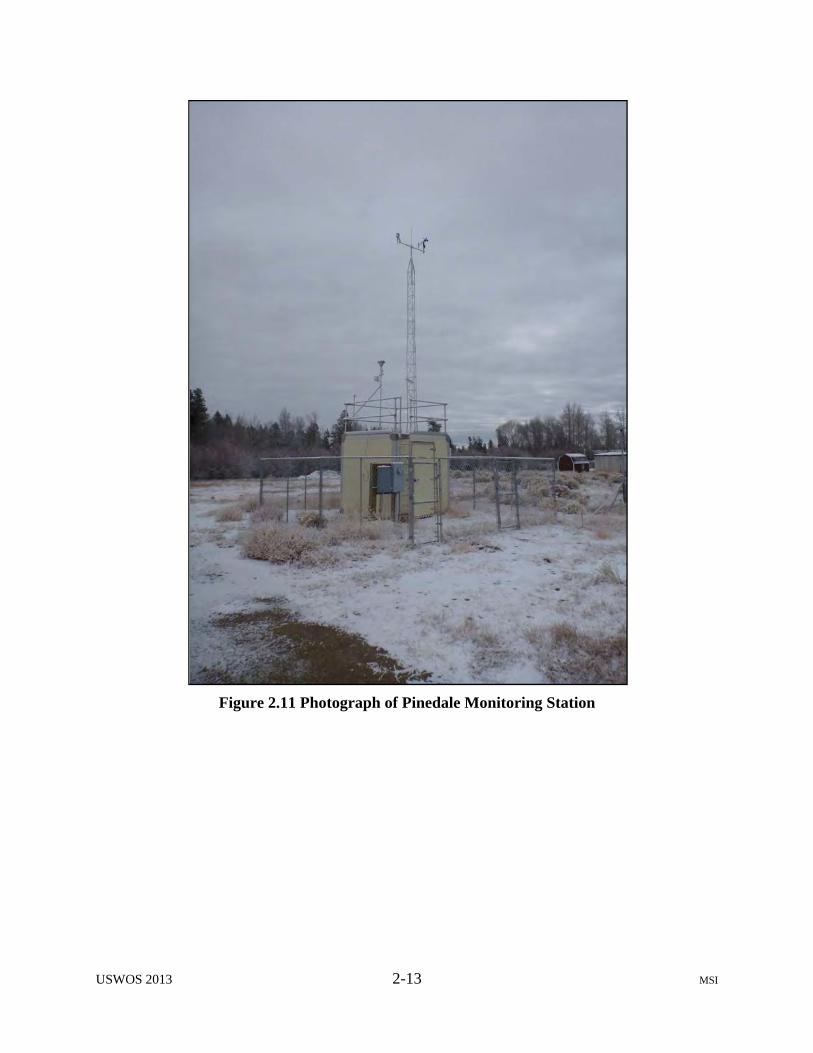
sulfur dioxide. Figure 2.11 presents a photograph of the Pinedale long-term monitoring site.
Figures 2.12 and 2.13 show the more extensive long-term monitoring station at Boulder. Figure
2.14 presents a photograph of the Boulder station interior.
USWOS 2013 2-13 MSI
Figure 2.11 Photograph of Pinedale Monitoring Station

USWOS 2013 2-14 MSI
Figure 2.12 Boulder Monitoring Site during UGWOS 2013
Figure 2.13 Boulder Meteorological Station with TUVR Sensors and UGWOS VOC
Sampling Tripod
USWOS 2013 2-15 MSI
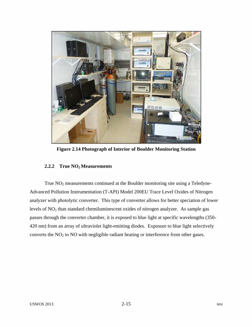
Figure 2.14 Photograph of Interior of Boulder Monitoring Station
2.2.2 True NO2 Measurements
True NO2 measurements continued at the Boulder monitoring site using a Teledyne-
Advanced Pollution Instrumentation (T-API) Model 200EU Trace Level Oxides of Nitrogen
analyzer with photolytic converter. This type of converter allows for better speciation of lower
levels of NO2 than standard chemiluminescent oxides of nitrogen analyzer. As sample gas
passes through the converter chamber, it is exposed to blue light at specific wavelengths (350-
420 nm) from an array of ultraviolet light-emitting diodes. Exposure to blue light selectively
converts the NO2 to NO with negligible radiant heating or interference from other gases.

USWOS 2013 2-16 MSI
NOy was measured at the Boulder site using a T-API Model T200U analyzer with a
Model 501Y converter mounted at the sample inlet point. This configuration allows for minimal
time delay between the sample inlet port and the remotely mounted molybdenum converter. The
system is designed to measure the concentration of NO, NO2 and other compounds that are too
unstable to be measured when brought in through the standard conventional ambient air sample
inlet system. Sampling the ambient air directly into the remote converter enables the conversion
of labile components of NOy which might normally be lost in a conventional system with longer
transit time between the sample inlet and the converter.
Total UV radiation (both incoming and reflected UV) was again measured at the Boulder
site as it was during UGWOS efforts since 2007 using a pair of Eppley TUVR sensors with one
pointed upward and the other pointed downward. Reflected UV provides a convenient indication
of the presence of snow cover on the ground surface at the Boulder site.
In addition, speciated VOC measurements are performed year-round using the TO-14
canister sampling method at the Boulder monitoring station. Canister samples were triggered
automatically when continuously monitored non-methane hydrocarbon (NMHC) levels exceeded
2.0 parts per million (ppm). Samples were submitted to Environmental Analytical Services
(EAS) laboratory after each event for modified TO-14 analysis as described in Section 3.2.
The Method TO-14 detailed hydrocarbon analysis (DHA) for PAMS compounds use
cryogenic trapping and a gas chromatograph with a flame ionization detector (FID) to measure
hydrocarbons collected in Summa canisters. A modified version of this method which followed
the protocol contained in the EPA Guidance Document “Technical Assistance Documents for
Sampling and Analysis of Ozone Precursors”, EPA/600-R-98/161, September 1998 was utilized.
This method was used to determining 90 individual hydrocarbons, including the 55 PAMS
compounds in air and gas samples.
USWOS 2013 2-17 MSI
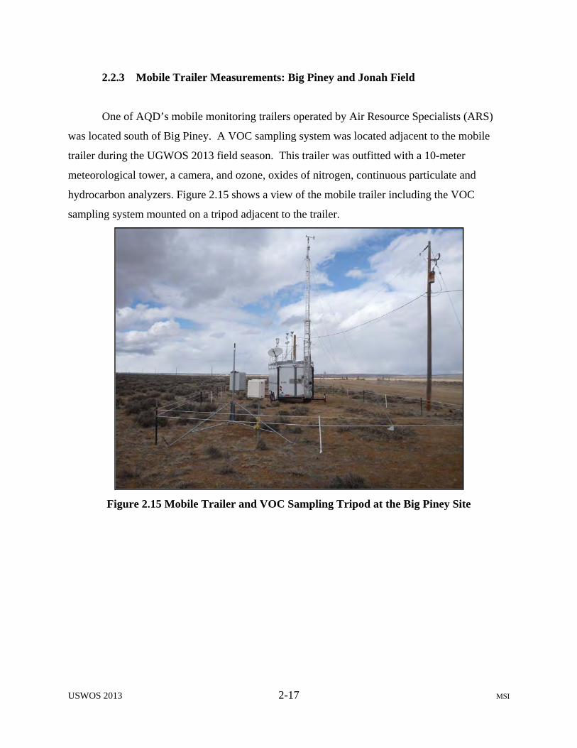
2.2.3 Mobile Trailer Measurements: Big Piney and Jonah Field
One of AQD’s mobile monitoring trailers operated by Air Resource Specialists (ARS)
was located south of Big Piney. A VOC sampling system was located adjacent to the mobile
trailer during the UGWOS 2013 field season. This trailer was outfitted with a 10-meter
meteorological tower, a camera, and ozone, oxides of nitrogen, continuous particulate and
hydrocarbon analyzers. Figure 2.15 shows a view of the mobile trailer including the VOC
sampling system mounted on a tripod adjacent to the trailer.
Figure 2.15 Mobile Trailer and VOC Sampling Tripod at the Big Piney Site
USWOS 2013 2-18 MSI
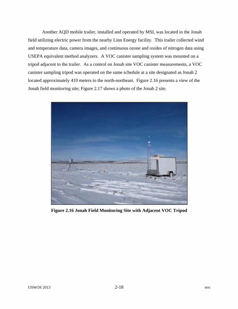
Another AQD mobile trailer, installed and operated by MSI, was located in the Jonah
field utilizing electric power from the nearby Linn Energy facility. This trailer collected wind
and temperature data, camera images, and continuous ozone and oxides of nitrogen data using
USEPA equivalent method analyzers. A VOC canister sampling system was mounted on a
tripod adjacent to the trailer. As a control on Jonah site VOC canister measurements, a VOC
canister sampling tripod was operated on the same schedule at a site designated as Jonah 2
located approximately 410 meters to the north-northeast. Figure 2.16 presents a view of the
Jonah field monitoring site; Figure 2.17 shows a photo of the Jonah 2 site.
Figure 2.16 Jonah Field Monitoring Site with Adjacent VOC Tripod
USWOS 2013 2-19 MSI
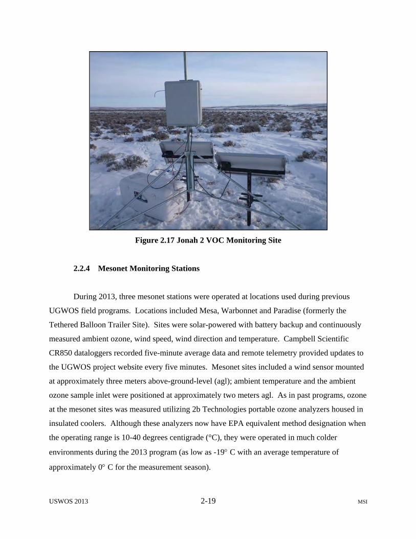
Figure 2.17 Jonah 2 VOC Monitoring Site
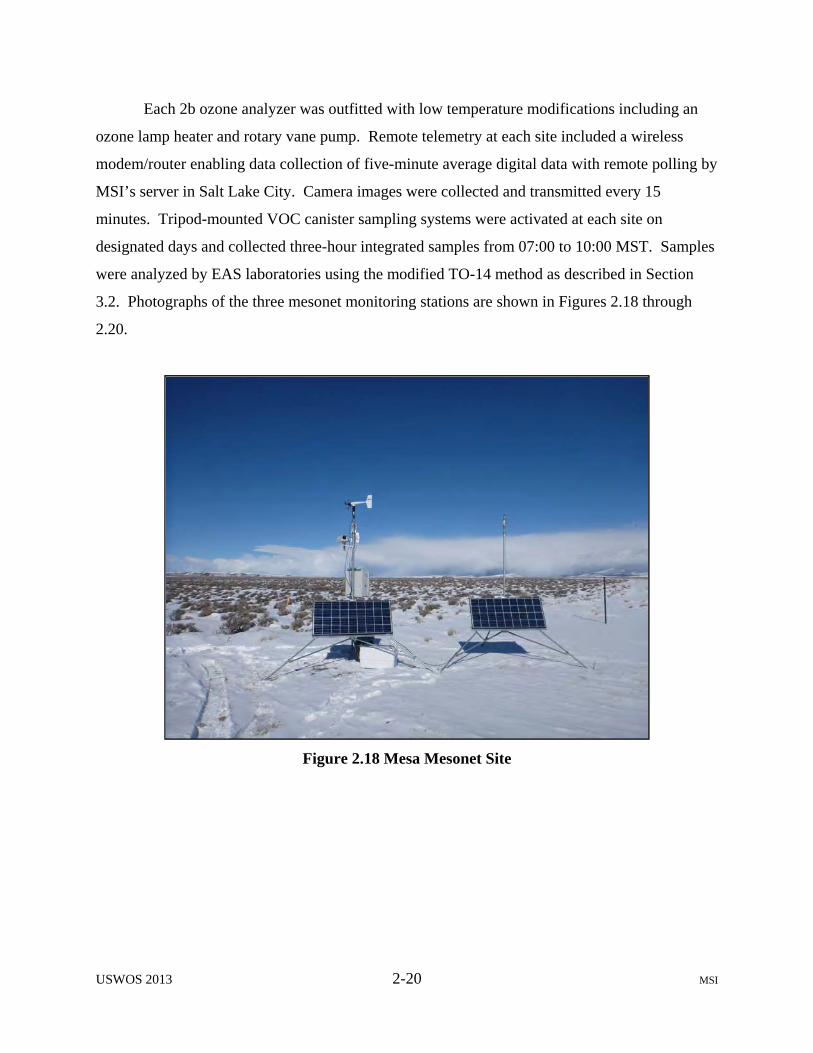
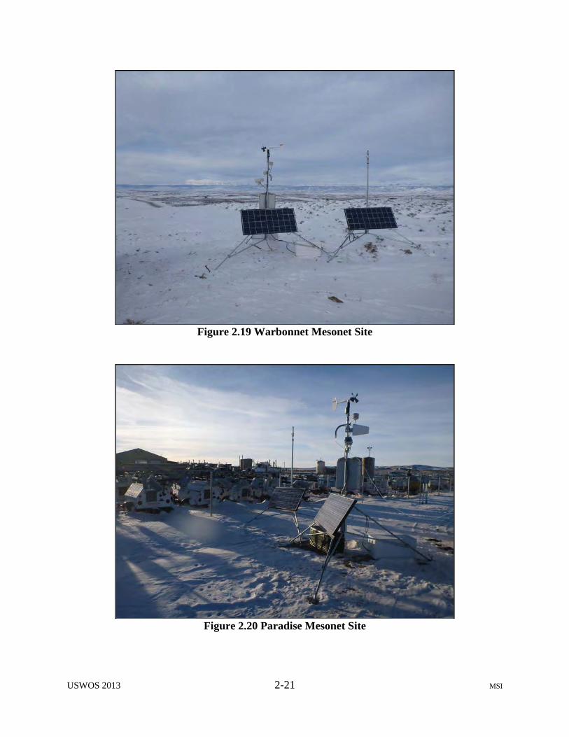
2.2.4 Mesonet Monitoring Stations
During 2013, three mesonet stations were operated at locations used during previous
UGWOS field programs. Locations included Mesa, Warbonnet and Paradise (formerly the
Tethered Balloon Trailer Site). Sites were solar-powered with battery backup and continuously
measured ambient ozone, wind speed, wind direction and temperature. Campbell Scientific
CR850 dataloggers recorded five-minute average data and remote telemetry provided updates to
the UGWOS project website every five minutes. Mesonet sites included a wind sensor mounted
at approximately three meters above-ground-level (agl); ambient temperature and the ambient
ozone sample inlet were positioned at approximately two meters agl. As in past programs, ozone
at the mesonet sites was measured utilizing 2b Technologies portable ozone analyzers housed in
insulated coolers. Although these analyzers now have EPA equivalent method designation when
the operating range is 10-40 degrees centigrade (°C), they were operated in much colder
environments during the 2013 program (as low as -19 C with an average temperature of
approximately 0 C for the measurement season).
USWOS 2013 2-20 MSI
Each 2b ozone analyzer was outfitted with low temperature modifications including an
ozone lamp heater and rotary vane pump. Remote telemetry at each site included a wireless
modem/router enabling data collection of five-minute average digital data with remote polling by
MSI’s server in Salt Lake City. Camera images were collected and transmitted every 15
minutes. Tripod-mounted VOC canister sampling systems were activated at each site on
designated days and collected three-hour integrated samples from 07:00 to 10:00 MST. Samples
were analyzed by EAS laboratories using the modified TO-14 method as described in Section
3.2. Photographs of the three mesonet monitoring stations are shown in Figures 2.18 through
2.20.
Figure 2.18 Mesa Mesonet Site
USWOS 2013 2-21 MSI
Figure 2.19 Warbonnet Mesonet Site
Figure 2.20 Paradise Mesonet Site

USWOS 2013 2-22 MSI
2.2.5 VOC Canister Sampling
Ambient air samples were collected in specially prepared stainless steel canisters using
the sub-atmospheric sampling method. An adjustable flow controller was used to control the
sample flow rate into the canister for a three-hour integrated sample with some negative pressure
still remaining in the canister at the end of the period. Canisters were typically loaded into each
system on the day before a sampling event. A solenoid valve was activated by a datalogger to
start the sampling process at the time selected (07:00-10:00) and closed at the end of the period.
Canisters were retrieved immediately following each event and shipped within a few days to
EAS laboratory for modified TO-14 analysis (description in Section 3.2) using gas
chromatography with a flame ionization detector (GC/FID).
The automated VOC canister sampling equipment owned by AQD was tested for
contamination prior to the start of the UGWOS field season by first flushing each system with
clean ambient air followed by ultra-pure air and then connecting a clean, evacuated canister to
each system. The canister with flow controller mounted was allowed to sample ultra-pure air for
a normal three-hour sampling period. Samples were sent to EAS laboratory for analysis to
confirm that each system was free of contamination. One of the ten sampling systems was
removed from service after a second round of purging, sampling zero air and analysis showed
some residual contamination. Based on the analytical results from each sample, the remaining
nine systems were declared clean.
VOC canister sampling systems were set up at Boulder, Juel Springs, Big Piney, Jonah
Field, and the Jonah Field control site designated as Jonah 2 as well as at the three mesonet sites
– Paradise, Mesa, and Warbonnet. The existing VOC canister sampling system at the Boulder
site operated in its normal configuration (which triggers a canister sample when the NMHC
value recorded by the site analyzer exceeds 2.0 ppm) during the UGWOS field season. An
additional tripod-mounted sampling system was placed at Boulder for conducting VOC canister
sampling on designated sampling days from 0700-1000.

USWOS 2013 2-23 MSI
Measurements of VOC’s were originally scheduled to be conducted during designated
IOPs. During UGWOS 2013, there were no designated IOPs, i.e. periods when elevated ambient
ozone concentrations were expected to develop. There were, however, five designated VOC
canister sampling days when conditions were forecast to be high pressure, light winds and sunny
skies which included the following dates: January 19, January 20, February 3, March 14, and
March 28, 2013.
2.2.6 miniSODARTM
The WDEQ Wind Explorer miniSODARTM was maintained and operated adjacent to the
Boulder monitoring station and continuously measured winds at the surface and aloft and
provided mixing height information up to approximately 250 meters. Figure 2.21 shows the
miniSODAR at its Boulder monitoring site location.
Figure 2.21 miniSODAR™

USWOS 2013 2-24 MSI
2.2.7 Ozonesondes/Radiosondes
During UGWOS 2013, MSI operated AQD’s ozonesonde/radiosonde upper air sounding
system based at the Boulder monitoring site to provide vertical profiles of ozone and
meteorology in the atmosphere above the study area. Radiosonde releases providing
meteorological information were planned for the morning flights and radiosondes with attached
ozonesondes to provide a vertical profile of ozone concentrations in the atmosphere above the
UGRB were scheduled for the afternoons. MSI dedicated an air quality technician to prepare the
sondes and conduct the soundings with the full-time UGWOS technician available as backup.
Both technicians were trained prior to the start of the field program.
The operational plan called for soundings to be performed during designated IOPs. Since
no IOPs were declared during UGWOS 2013, upper air soundings were limited to test runs
conducted on January 17, 2013.
2.3 Designated VOC Canister Sampling Days
During UGWOS 2013, weather and ozone development forecasts were issued daily to
identify periods when conditions would be conducive to producing elevated ambient ozone
concentrations in the study area. These periods would then be treated as IOP’s when additional
field activities, namely VOC canister sampling at eight (8) sites and ozone/radiosonde balloon
launches, would take place. During UGWOS 2013, conditions conducive to significant elevated
ozone formation never materialized and no IOP’s were forecast. Instead, in order to provide
additional speciated hydrocarbon data for the study domain, VOC canister sampling days were
designated based on a forecast of stable, high pressure conditions with light winds and sunny
skies.
This section describes the weather and ozone development outlooks issued daily to
forecast elevated ozone episodes as well as the synoptic weather summaries of conditions during
the designated VOC canister sampling days during UGWOS 2013.
USWOS 2013 2-25 MSI
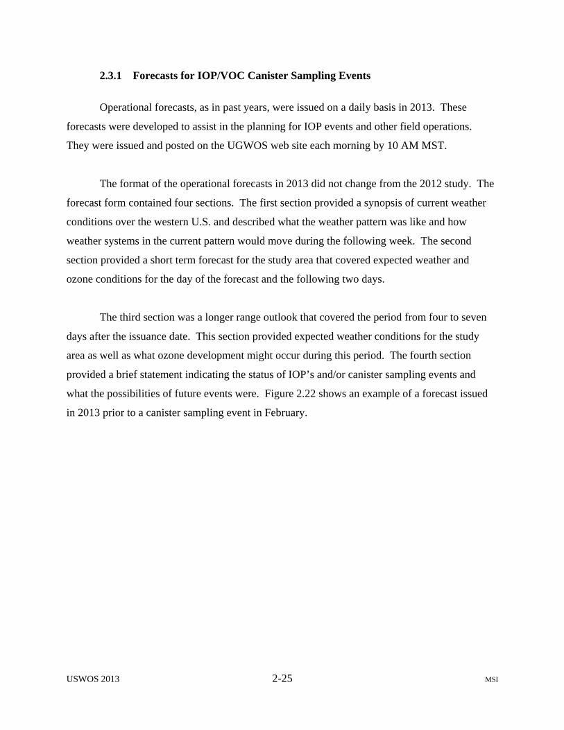
2.3.1 Forecasts for IOP/VOC Canister Sampling Events
Operational forecasts, as in past years, were issued on a daily basis in 2013. These
forecasts were developed to assist in the planning for IOP events and other field operations.
They were issued and posted on the UGWOS web site each morning by 10 AM MST.
The format of the operational forecasts in 2013 did not change from the 2012 study. The
forecast form contained four sections. The first section provided a synopsis of current weather
conditions over the western U.S. and described what the weather pattern was like and how
weather systems in the current pattern would move during the following week. The second
section provided a short term forecast for the study area that covered expected weather and
ozone conditions for the day of the forecast and the following two days.
The third section was a longer range outlook that covered the period from four to seven
days after the issuance date. This section provided expected weather conditions for the study
area as well as what ozone development might occur during this period. The fourth section
provided a brief statement indicating the status of IOP’s and/or canister sampling events and
what the possibilities of future events were. Figure 2.22 shows an example of a forecast issued
in 2013 prior to a canister sampling event in February.

USWOS 2013 2-26 MSI
Figure 2.22 Example Weather Outlook

USWOS 2013 2-27 MSI
2.3.2 Synoptic Weather Summaries of Canister Sampling Events
For 2013 there were no IOP’s declared. However, there were four periods when VOC
canister sampling occurred. The samples were taken in the morning hours between 0700-1000.
The first sampling event occurred during the mornings on two consecutive days and the
following three events were each conducted during the mornings on a single day.
January 19-20, 2013
High pressure covered much of the western United States (US) on both days, with little
change in the pattern from day to day, although pressure increased slightly from January 19 to
20. At the 700 millibar (mb) level, a high pressure ridge stretched from the Washington
coastline south to western Arizona. A broad trough of low pressure was centered in northeastern
Canada. The jet stream between the pressure centers pushed southeast out of British Columbia
into the northern Plains and across the Great Lakes region. Wind speeds at 700 mb were as high
as 28 meters per second (mps) across Montana and North Dakota, but over western Wyoming
speeds were approximately 3 to 8 mps from the northwest.
At the surface, high pressure was covering much of southern Idaho, northern Nevada and
Utah, and western Colorado and Wyoming. The surface pressure strengthened slightly over the
study area from approximately 1032 mb on January 19 to 1038 mb on January 20.
Winds were light at the surface both mornings with speeds mostly under 4 mps. Winds
were predominately from the northwest on January 19 but variable on January 20. Temperatures
across the study area during the sampling on January 19 ranged from approximately -19⁰C to -
5⁰C. Temperatures on January 20 were similar to the previous day temperatures, ranging from
-19⁰C to -8⁰C. These temperatures were just slightly higher than the morning lows which
occurred in the hour or two prior to when sampling began.
USWOS 2013 2-28 MSI
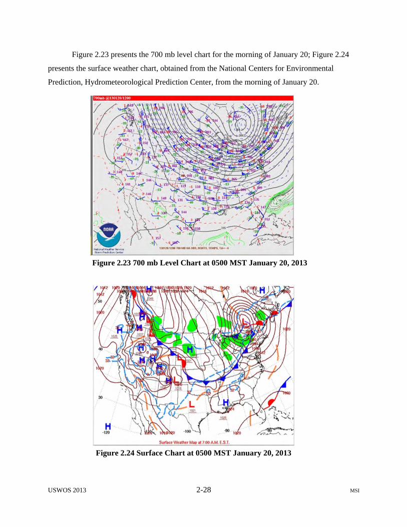
Figure 2.23 presents the 700 mb level chart for the morning of January 20; Figure 2.24
presents the surface weather chart, obtained from the National Centers for Environmental
Prediction, Hydrometeorological Prediction Center, from the morning of January 20.
Figure 2.24 Surface Chart at 0500 MST January 20, 2013
Figure 2.23 700 mb Level Chart at 0500 MST January 20, 2013
USWOS 2013 2-29 MSI
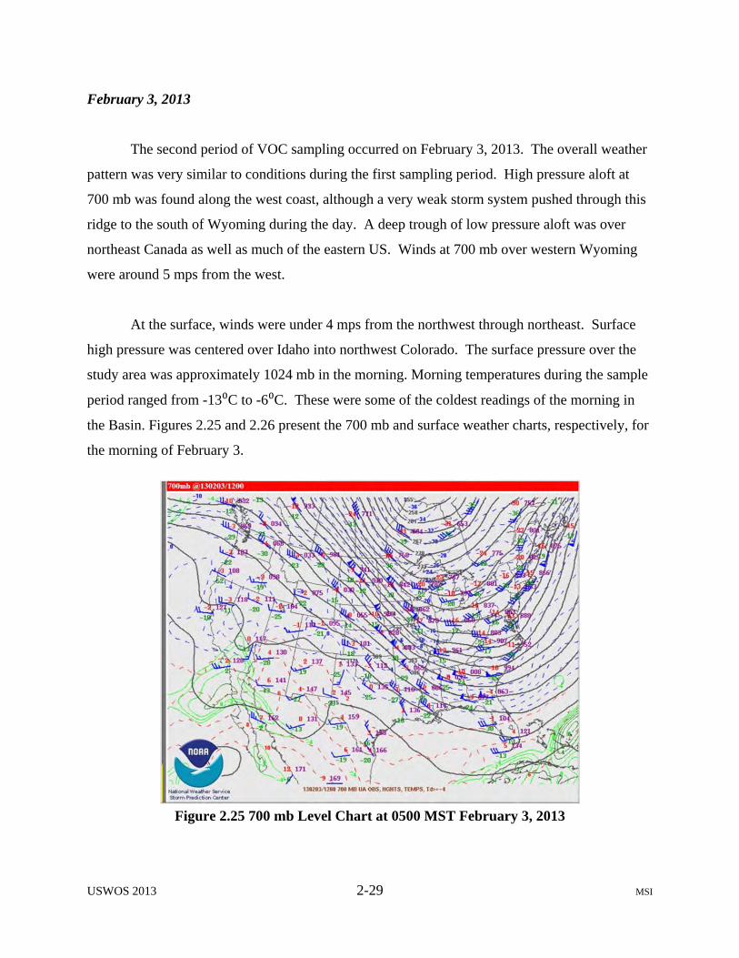
February 3, 2013
The second period of VOC sampling occurred on February 3, 2013. The overall weather
pattern was very similar to conditions during the first sampling period. High pressure aloft at
700 mb was found along the west coast, although a very weak storm system pushed through this
ridge to the south of Wyoming during the day. A deep trough of low pressure aloft was over
northeast Canada as well as much of the eastern US. Winds at 700 mb over western Wyoming
were around 5 mps from the west.
At the surface, winds were under 4 mps from the northwest through northeast. Surface
high pressure was centered over Idaho into northwest Colorado. The surface pressure over the
study area was approximately 1024 mb in the morning. Morning temperatures during the sample
period ranged from -13⁰C to -6⁰C. These were some of the coldest readings of the morning in
the Basin. Figures 2.25 and 2.26 present the 700 mb and surface weather charts, respectively, for
the morning of February 3.
Figure 2.25 700 mb Level Chart at 0500 MST February 3, 2013

USWOS 2013 2-30 MSI
March 14, 2013
The third period of VOC sampling occurred on March 14, 2013. Again, the weather
pattern was similar to the first and second sampling periods. High pressure aloft was stronger
and closer to Wyoming. The ridge line was lying from Idaho south to the high pressure center
located over the California/Nevada/Arizona triple point. A trough of low pressure at 700 mb
stretched from the low center in southeast Canada down the east coast to Florida. Winds over
western Wyoming at 700 mb were at 10 to 13 mps from the northwest.
Figure 2.26 Surface Chart at 0500 MST February 3, 2013

USWOS 2013 2-31 MSI
Surface conditions were similar to the previous sample dates as well with high pressure
centered over central Idaho, across western Wyoming into western Colorado. The surface
pressure over the study area was approximately 1026 mb. Winds were very light with speeds
between 1 and 2 mps. Directions were variable but tended to be from the northwest to northeast.
Temperatures were warmer than previous sampling periods and ranged from -6⁰C to 0⁰ C at the
beginning of sampling, warming to 0⁰C to 5⁰ C by 10 AM. Figure 2.27 presents the 700 mb
weather chart for the morning of March 14. Figure 2.28 presents the surface weather chart for
the morning of March 14.
Figure 2.27 700 mb Level Chart at 0500 MST March 14, 2013
USWOS 2013 2-32 MSI
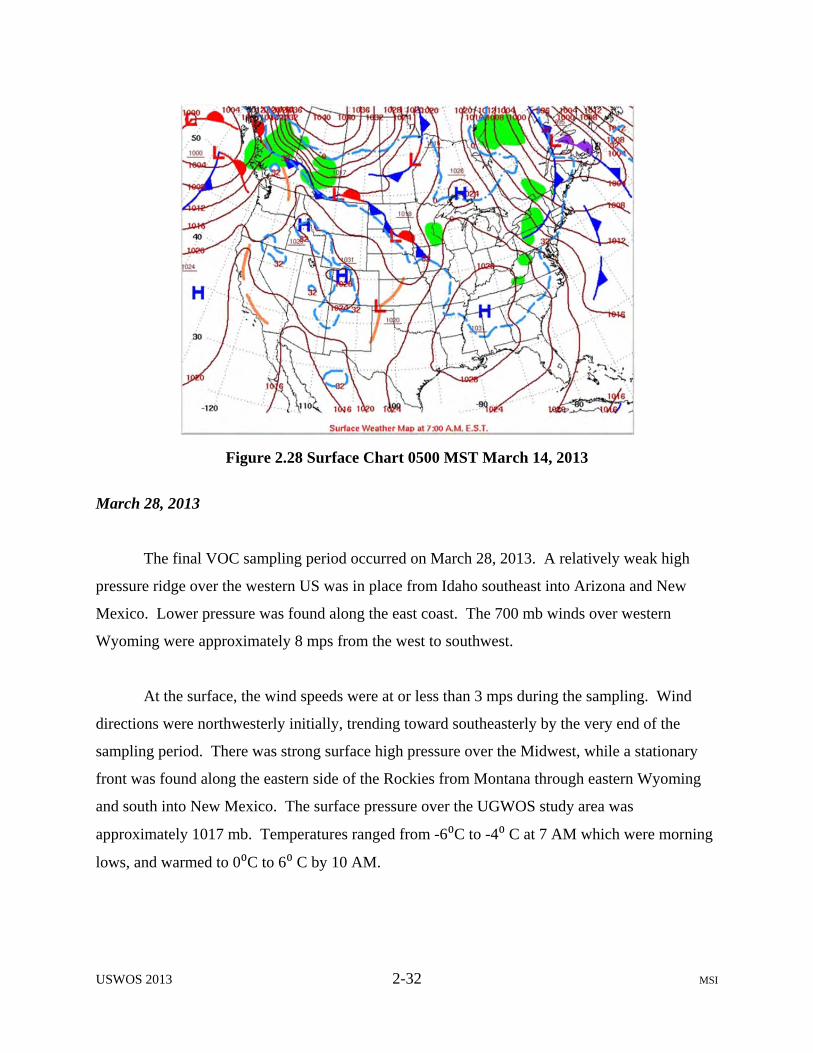
Figure 2.28 Surface Chart 0500 MST March 14, 2013
March 28, 2013
The final VOC sampling period occurred on March 28, 2013. A relatively weak high
pressure ridge over the western US was in place from Idaho southeast into Arizona and New
Mexico. Lower pressure was found along the east coast. The 700 mb winds over western
Wyoming were approximately 8 mps from the west to southwest.
At the surface, the wind speeds were at or less than 3 mps during the sampling. Wind
directions were northwesterly initially, trending toward southeasterly by the very end of the
sampling period. There was strong surface high pressure over the Midwest, while a stationary
front was found along the eastern side of the Rockies from Montana through eastern Wyoming
and south into New Mexico. The surface pressure over the UGWOS study area was
approximately 1017 mb. Temperatures ranged from -6⁰C to -4⁰ C at 7 AM which were morning
lows, and warmed to 0⁰C to 6⁰ C by 10 AM.
USWOS 2013 2-33 MSI
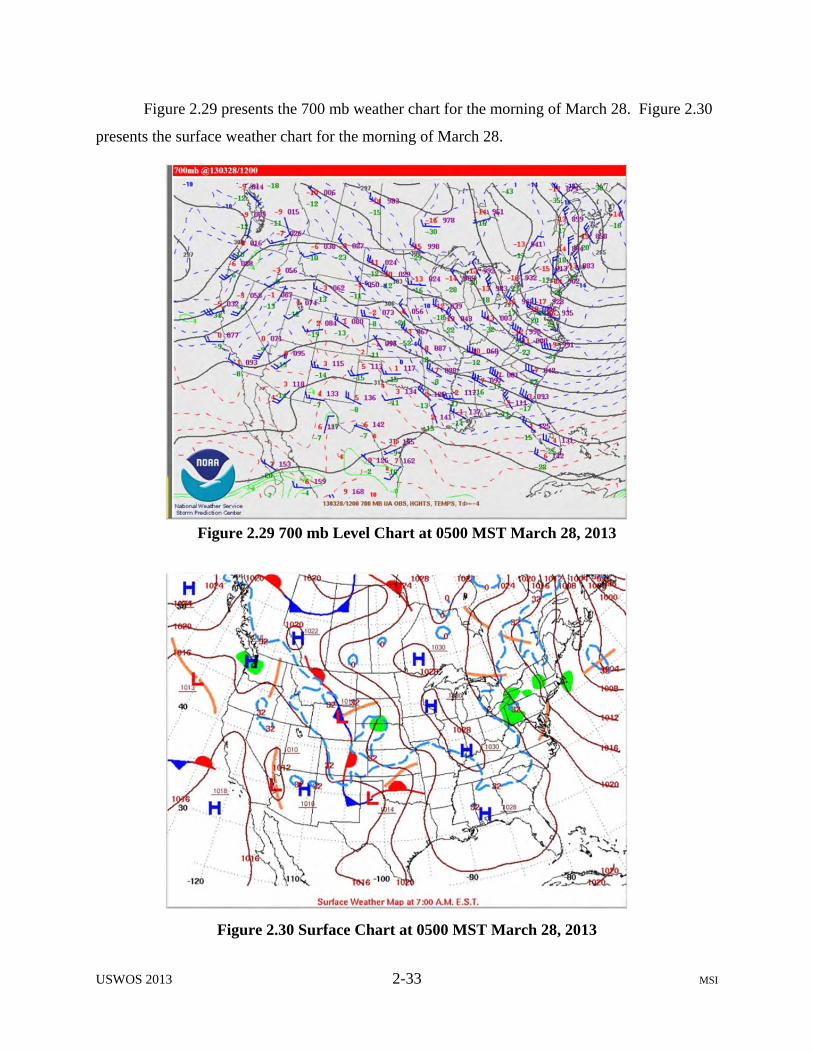
Figure 2.29 presents the 700 mb weather chart for the morning of March 28. Figure 2.30
presents the surface weather chart for the morning of March 28.
Figure 2.29 700 mb Level Chart at 0500 MST March 28, 2013
Figure 2.30 Surface Chart at 0500 MST March 28, 2013
UGWOS 2013 3-1 MSI
3.0 DATA QUALITY ASSURANCE, VALIDATION AND ARCHIVING
A primary study objective was to produce a validated data set from the field
measurements that is well defined and documented. The data management system used,
Microsoft Access, was designed to be straightforward and easy for users to obtain data and
provide updates. All data were quality-assured and submitted to MSI’s UGWOS Data Manager
for entry to the project database. A brief summary of procedures used is provided below.
3.1 Database Management
The overall goal of the data management effort was to create a well-documented system
such that data could be readily input and easily accessed from the database. A Monitoring and
Quality Assurance document was prepared and approved by all the project participants and can
be found on the AQD website.
Each of the participants that provided data was responsible for reviewing and validating their
respective data to Level 1 as described in Watson, et. al. (2001)1. This included flagging data
during instrument downtime and performance tests, applying any adjustments for calibration
deviation, investigating extreme values, and applying appropriate flags. Quality control (QC)
codes used for the UGWOS data set are presented in Table 3-1. QC codes include simple
validation codes as well as AQS null codes developed by the EPA.
1 Watson, J.G.; Turpin, B.J.; and Chow, J.C. (2001). The measurement process: Precision, accuracy, and validity. In Air Sampling Instruments for Evaluation of Atmospheric Contaminants, Ninth Edition, 9th ed., B.S. Cohen and C.S.J. McCammon, Eds. American Conference of Governmental Industrial Hygienists, Cincinnati, OH, pp. 201-216.

UGWOS 2013 3-2 MSI
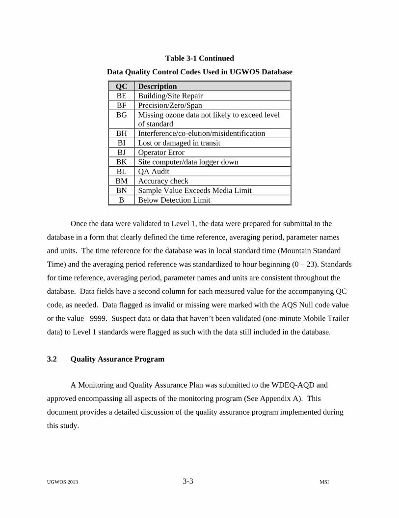
Table 3-1
Data Quality Control Codes Used in UGWOS Database
QC Description V Valid Data M Missing Data I Invalid Data S Suspect Data. Data appears to be a data spike or outside normal data rangeU Data which has not been validated - User is responsible for validation.
N Instrument Noise detected in sub hourly data used to create hourly average
B Below Detection Limit AA Sample Pressure out of Limits AB Technician Unavailable AC Construction/Repairs in Area AD Shelter Storm Damage AE Shelter Temperature Outside Limits AF Scheduled but not Collected AG Sample Time out of Limits AH Sample Flow Rate out of Limits AI Insufficient Data (cannot calculate) AJ Filter Damage AK Filter Leak AL Voided by Operator AM Miscellaneous Void AN Machine Malfunction AO Bad Weather AP Vandalism AQ Collection Error AR Lab Error AS Poor Quality Assurance Results AT Calibration AU Monitoring Waived AV Power Failure AW Wildlife Damage AX Precision Check AY Q C Control Points (zero/span) AZ Q C Audit BA Maintenance/Routine Repairs BB Unable to Reach Site BC Multi-point Calibration BD Auto Calibration
UGWOS 2013 3-3 MSI
Table 3-1 Continued
Data Quality Control Codes Used in UGWOS Database
QC Description BE Building/Site Repair BF Precision/Zero/Span BG Missing ozone data not likely to exceed level
of standard BH Interference/co-elution/misidentification BI Lost or damaged in transit BJ Operator Error BK Site computer/data logger down BL QA Audit BM Accuracy check BN Sample Value Exceeds Media Limit B Below Detection Limit
Once the data were validated to Level 1, the data were prepared for submittal to the
database in a form that clearly defined the time reference, averaging period, parameter names
and units. The time reference for the database was in local standard time (Mountain Standard
Time) and the averaging period reference was standardized to hour beginning (0 – 23). Standards
for time reference, averaging period, parameter names and units are consistent throughout the
database. Data fields have a second column for each measured value for the accompanying QC
code, as needed. Data flagged as invalid or missing were marked with the AQS Null code value
or the value –9999. Suspect data or data that haven’t been validated (one-minute Mobile Trailer
data) to Level 1 standards were flagged as such with the data still included in the database.
3.2 Quality Assurance Program
A Monitoring and Quality Assurance Plan was submitted to the WDEQ-AQD and
approved encompassing all aspects of the monitoring program (See Appendix A). This
document provides a detailed discussion of the quality assurance program implemented during
this study.
UGWOS 2013 3-4 MSI
As part of the quality assurance program, quality control procedures were implemented to
assess and maintain control of the quality of the data collected. A summary of key elements of
the QC program for each measurement is presented in the remainder of this section.
All UGWOS equipment underwent a complete checkout and acceptance prior to the start
of monitoring. Standard Operating Procedures (SOPs) for measurements were completed prior to
the start of monitoring.
All UGWOS 2013 ozone and oxides of nitrogen analyzers were routinely checked using
a traceable transfer standard or reference gas following operating procedures consistent with
EPA guidelines. Ozone transfer standards were verified prior to the start of the program and
again at the end by checks against a primary standard maintained at MSI’s instrumentation
laboratory in Salt Lake City. MSI’s primary ozone standard was last verified by USEPA Region
VIII on January 3, 2013. The oxides of nitrogen analyzer at the Jonah Field site was checked
using an EPA Protocol Nitric Oxide calibration gas. Mass flow controller flows in the calibrator
used at the Jonah Field site were calibrated at the start of the field program.
Data from mesonet sites, the Jonah Field site and long-term monitoring sites operated by
MSI were retrieved remotely at least every 15 minutes. Data from other sites in the UGRB were
retrieved hourly. Data updates were posted on the UGWOS website immediately after retrieval
and were available to project participants. Data from all sites in the project area were reviewed
and inspected daily to confirm normal operation and identify outliers or indications that
instrumentation needed attention or repair. MSI’s air quality technician, stationed in the
Pinedale, Wyoming area for the duration of the field program, was able to respond to and rectify
problems quickly which enhanced data recovery.
UGWOS 2013 3-5 MSI
WDEQ tripod-mounted portable VOC sampling systems were leak checked, cleaned and
checked for contamination prior to the start of the UGWOS 2013 study. System components
were first purged with clean ambient (humidified) air and then ultrapure air before testing. VOC
canisters were installed in each system, allowed to sample ultrapure air through the system inlet,
and sent to the analytical laboratory for analysis to confirm that systems were free of
contamination. During testing and on specified sampling days during the field program, a field
sample data sheet was generated for each VOC canister indicating sample ID, sample date and
time, and canister start and stop pressure. VOC canisters were sent back to the laboratory for
analysis following each sampling event accompanied by a chain-of-custody form. Analysis was
performed using Method TO-14, Detailed Hydrocarbon Analysis (DHA) for PAMS Compounds.
EAS performed a modified version of the method following the protocols found in EPA’s
document, “Technical Assistance Document for Sampling and Analysis of Ozone Precursors”,
(EPA/600-R-98/161, September 1998). The method was used to determine 90 individual
hydrocarbons including the 55 PAMS compounds in air and gas samples. The Method TO-14
DHA compound list, method detection limits, limits of quantification and other laboratory
criteria are presented in Table 3-2.
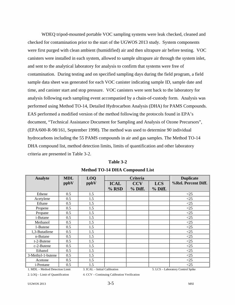
Table 3-2
Method TO-14 DHA Compound List
Analyte MDL ppbV
LOQ ppbV
Criteria Duplicate %Rel. Percent Diff.ICAL
% RSD CCV
% Diff. LCS
% Diff. Ethene 0.5 1.5 <25
Acetylene 0.5 1.5 <25 Ethane 0.5 1.5 <25 Propene 0.5 1.5 <25 Propane 0.5 1.5 <25 i-Butane 0.5 1.5 <25 Methanol 0.5 1.5 <25 1-Butene 0.5 1.5 <25
1,3-Butadiene 0.5 1.5 <25 n-Butane 0.5 1.5 <25
t-2-Butene 0.5 1.5 <25 c-2-Butene 0.5 1.5 <25
Ethanol 0.5 1.5 <25 3-Methyl-1-butene 0.5 1.5 <25
Acetone 0.5 1.5 <25 i-Pentane 0.5 1.5 <25
1. MDL – Method Detection Limit 3. ICAL – Initial Calibration 5. LCS – Laboratory Control Spike
2. LOQ – Limit of Quantification 4. CCV – Continuing Calibration Verification
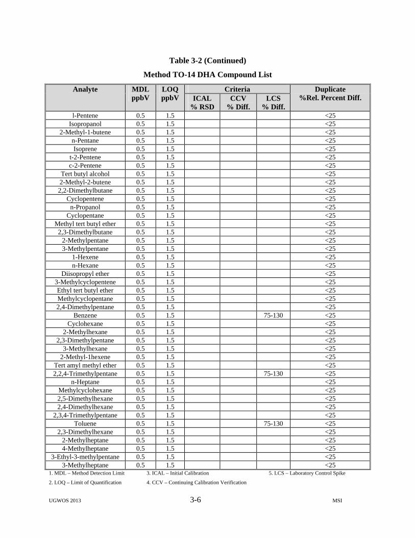
UGWOS 2013 3-6 MSI
Table 3-2 (Continued)
Method TO-14 DHA Compound List
Analyte MDL ppbV
LOQ ppbV
Criteria Duplicate %Rel. Percent Diff. ICAL
% RSD CCV
% Diff. LCS
% Diff. l-Pentene 0.5 1.5 <25
Isopropanol 0.5 1.5 <25 2-Methyl-1-butene 0.5 1.5 <25
n-Pentane 0.5 1.5 <25 Isoprene 0.5 1.5 <25
t-2-Pentene 0.5 1.5 <25 c-2-Pentene 0.5 1.5 <25
Tert butyl alcohol 0.5 1.5 <25 2-Methyl-2-butene 0.5 1.5 <25 2,2-Dimethylbutane 0.5 1.5 <25
Cyclopentene 0.5 1.5 <25 n-Propanol 0.5 1.5 <25
Cyclopentane 0.5 1.5 <25 Methyl tert butyl ether 0.5 1.5 <25 2,3-Dimethylbutane 0.5 1.5 <25
2-Methylpentane 0.5 1.5 <25 3-Methylpentane 0.5 1.5 <25
1-Hexene 0.5 1.5 <25n-Hexane 0.5 1.5 <25
Diisopropyl ether 0.5 1.5 <253-Methylcyclopentene 0.5 1.5 <25Ethyl tert butyl ether 0.5 1.5 <25Methylcyclopentane 0.5 1.5 <252,4-Dimethylpentane 0.5 1.5 <25
Benzene 0.5 1.5 75-130 <25Cyclohexane 0.5 1.5 <25
2-Methylhexane 0.5 1.5 <252,3-Dimethylpentane 0.5 1.5 <25
3-Methylhexane 0.5 1.5 <252-Methyl-1hexene 0.5 1.5 <25
Tert amyl methyl ether 0.5 1.5 <252,2,4-Trimethylpentane 0.5 1.5 75-130 <25
n-Heptane 0.5 1.5 <25Methylcyclohexane 0.5 1.5 <252,5-Dimethylhexane 0.5 1.5 <252,4-Dimethylhexane 0.5 1.5 <25
2,3,4-Trimethylpentane 0.5 1.5 <25Toluene 0.5 1.5 75-130 <25
2,3-Dimethylhexane 0.5 1.5 <252-Methylheptane 0.5 1.5 <254-Methylheptane 0.5 1.5 <25
3-Ethyl-3-methylpentane 0.5 1.5 <253-Methylheptane 0.5 1.5 <25
1. MDL – Method Detection Limit 3. ICAL – Initial Calibration 5. LCS – Laboratory Control Spike
2. LOQ – Limit of Quantification 4. CCV – Continuing Calibration Verification

UGWOS 2013 3-7 MSI
Table 3-2 (Continued)
Method TO-14 DHA Compound List
Analyte MDL ppbV
LOQ ppbV
Criteria Duplicate %Rel. Percent
Diff. ICAL
% RSD CCV
% Diff. LCS
% Diff. 2-Methyl-1-heptene 0.5 1.5 <25
n-Octane 0.5 1.5 <25 Ethylbenzene 0.5 1.5 <25 m,p-xylene 0.5 1.5 75-130 <25
Styrene 0.5 1.5 <25 o-xylene 0.5 1.5 75-130 <25 1-Nonene 0.5 1.5 <25 N-Nonane 0.5 1.5 <25
i-Propylbenzene 0.5 1.5 <25 n-propylbenzene 0.5 1.5 <25
a-Pinene 0.5 1.5 <25 3-Ethyltoluene 0.5 1.5 <25 4-Ethyltoluene 0.5 1.5 <25
1,3,5-Trimethylbenzene 0.5 1.5 75-130 2-Ethyltoluene 0.5 1.5 <25
b-Pinene 0.5 1.5 <25 1,2,4-Trimethlybenzene 0.5 1.5 <25
n-Decane 0.5 1.5 <251,2,3-Trimethlybenzene 0.5 1.5 <25
Indan 0.5 1.5 <25d-Limonene 0.5 1.5 <25
1,3-Diethylbenzene 0.5 1.5 <251,4-Diethylbenzene 0.5 1.5 <25
n-Butylbenzene 0.5 1.5 <251,4-Dimethyl-2-ethylbenzene 0.5 1.5 <251,3-Dimethyl-4-ethylbenzene 0.5 1.5 <251,2-Dimethyl-4-ethylbenzene 0.5 1.5 <25
Undecane 0.5 1.5 <251,2,4,5-Tetramethylbenzene 0.5 1.5 <251,2,3,5-Tetramethylbenzene 0.5 1.5 <25
Napthalene 0.5 1.5 <25Dodecane 0.5 1.5 <25
1. MDL – Method Detection Limit 3. ICAL – Initial Calibration 5. LCS – Laboratory Control Spike
2. LOQ – Limit of Quantification 4. CCV – Continuing Calibration Verification
The FID is calibrated using propane and hexane and the responses of individual
hydrocarbons are calculated against these compounds in ppbC according to the procedure
described in the guidance document.
UGWOS 2013 3-8 MSI
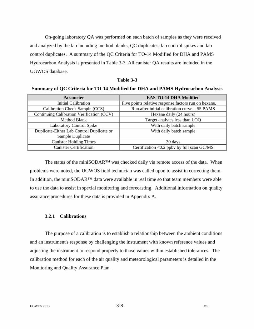
On-going laboratory QA was performed on each batch of samples as they were received
and analyzed by the lab including method blanks, QC duplicates, lab control spikes and lab
control duplicates. A summary of the QC Criteria for TO-14 Modified for DHA and PAMS
Hydrocarbon Analysis is presented in Table 3-3. All canister QA results are included in the
UGWOS database.
Table 3-3
Summary of QC Criteria for TO-14 Modified for DHA and PAMS Hydrocarbon Analysis
Parameter EAS TO-14 DHA Modified Initial Calibration Five points relative response factors run on hexane.
Calibration Check Sample (CCS) Run after initial calibration curve – 55 PAMS Continuing Calibration Verification (CCV) Hexane daily (24 hours)
Method Blank Target analytes less than LOQ Laboratory Control Spike With daily batch sample
Duplicate-Either Lab Control Duplicate or Sample Duplicate
With daily batch sample
Canister Holding Times 30 days Canister Certification Certification <0.2 ppbv by full scan GC/MS
The status of the miniSODAR™ was checked daily via remote access of the data. When
problems were noted, the UGWOS field technician was called upon to assist in correcting them.
In addition, the miniSODAR™ data were available in real time so that team members were able
to use the data to assist in special monitoring and forecasting. Additional information on quality
assurance procedures for these data is provided in Appendix A.
3.2.1 Calibrations
The purpose of a calibration is to establish a relationship between the ambient conditions
and an instrument's response by challenging the instrument with known reference values and
adjusting the instrument to respond properly to those values within established tolerances. The
calibration method for each of the air quality and meteorological parameters is detailed in the
Monitoring and Quality Assurance Plan.
UGWOS 2013 3-9 MSI
Meteorological sensors were calibrated at the beginning and end of the study. Wind
speed sensors were calibrated using an R.M. Young constant rpm motor simulating wind speeds
at several points across the sensor’s operating range. Wind direction sensors were calibrated by
confirming orientation and checking responses at standard increments. Temperature sensors
were calibrated using water/ice baths.
Air quality analyzers were calibrated at the start of the UGWOS 2013 study and
calibration was verified again at the end. Zero/span/one point QC checks were conducted
approximately every two-weeks during the study.
3.2.2 Quality Assurance Audits
As part of the UGWOS quality assurance program, an independent audit program was
implemented to verify the site operations and data accuracy. The auditor and the equipment used
for the audit were independent of the measurement program. Audits were performed in
accordance with the principles set forth by the US EPA.
3.2.2.1 Performance Audits
Air Quality Variables
Mesonet ozone analyzers and ozonesonde measurements were audited using a Dasibi
Model 1008 PC transfer standard that is certified against T&B Systems’ primary standard
maintained following EPA’s guidelines at their office in Valencia, California. The Model 1008
PC is an ozone photometer equipped with self-contained zero air and ozone generation. For the
mesonet audits, the transfer standard was operated within the SUV used during the audit. The
transfer standard was powered using a true sine wave inverter, and was allowed to warm up prior
to the audit to a point where the temperature within the standard’s photometer cell was relatively
stable. Ozone concentrations were fed to the mesonet site’s sample inlet with an 8-foot ¼”
Teflon line, with a venting tee placed at the inlet. The airflow to the tee was approximately 2
lpm, minimizing residence time within the line.
UGWOS 2013 3-10 MSI
Gaseous analyzers at the UGWOS Jonah site were audited using a Teledyne Advanced
Pollution Instrumentation (T-API) Model 700EU mass flow-controlled dilution calibrator to
dilute known concentrations of audit gas with zero air and create known audit concentrations.
EPA protocol gases from Scott-Marrin were used. The T-API calibrator is also equipped with an
integrated photometer which was used as an ozone transfer standard. The T-API photometer is
certified quarterly against a primary photometer maintained by T&B Systems following EPA
guidelines.
Wind speed sensors were audited using an R.M. Young constant rpm motor simulating
wind speeds at several points across the sensor’s operating range. Wind direction sensors were
audited by checking the sensor orientation and responses in 30 or 45 increments using the
marks on the wind direction sensor. The wind speed starting threshold was checked using an
R.M. Young torque disc. Wind sensors were left in place during the audit to minimize the audit
effort and prevent any accidental damage to the monitoring system. This setup has the potential
to result in decreased precision of the wind direction checks, particularly under windy or
extremely cold conditions. In addition, wind direction starting thresholds could not be directly
checked, though the bearings were inspected by feel.
Temperature sensors were audited using a water bath and a certified audit sensor. Three
points were checked using an ice bath and two upscale water bath points between 10oC and
30oC. For sites where the ambient temperature during the audit was lower than -10C, ambient
temperatures were cold enough during the audit to provide an additional check at a sub-zero
level using a collocated temperature sensor.
Ozone audit results are summarized in Table 3-4. Note that site readings consist of five-
minute averaged “adjusted” values which take into account results from the most recent
performance checks conducted by MSI. All of the results showed agreement within about 4%,
easily meeting the audit criteria of ±10%. Audits of the mesonet meteorological systems
revealed that all wind and temperature sensors were operating correctly.
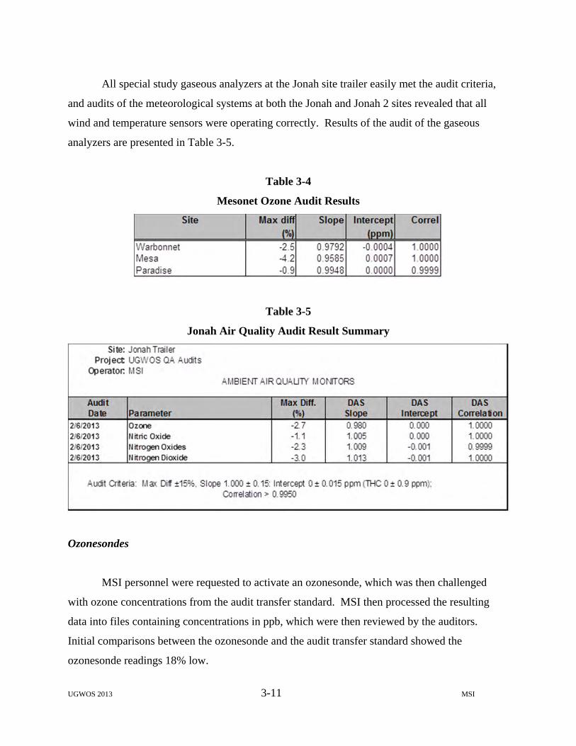
UGWOS 2013 3-11 MSI
All special study gaseous analyzers at the Jonah site trailer easily met the audit criteria,
and audits of the meteorological systems at both the Jonah and Jonah 2 sites revealed that all
wind and temperature sensors were operating correctly. Results of the audit of the gaseous
analyzers are presented in Table 3-5.
Table 3-4
Mesonet Ozone Audit Results
Table 3-5
Jonah Air Quality Audit Result Summary
Ozonesondes
MSI personnel were requested to activate an ozonesonde, which was then challenged
with ozone concentrations from the audit transfer standard. MSI then processed the resulting
data into files containing concentrations in ppb, which were then reviewed by the auditors.
Initial comparisons between the ozonesonde and the audit transfer standard showed the
ozonesonde readings 18% low.
UGWOS 2013 3-12 MSI
After review of both the ozonesonde operations and the audit equipment (including
verification of the audit concentrations using the independently audited Boulder ozone analyzer),
it was determined that the most likely parameter affecting the ozonesonde readings was the
ozonesonde sample flow rate (in seconds per 100 ml) used to initiate a given ozonesonde flight,
which is directly proportional to the calculated ozone concentration. The value stamped on the
ozonesonde pump was 28.0 - 28.2 s/100ml, whereas the value measured by the factory-supplied
bubble flow meter (measured by recording the time in seconds for the bubble to travel 100 ml)
was 23.5 s/100ml – a discrepancy that was unusually high based on the experience of the
auditors. Using an available MSI mass flow meter, the operating technician measured the flow
as 28.4 s/100ml (corrected to actual conditions), very close to the factory value. This flow rate
was further confirmed using an audit Bios flow meter. Further investigation revealed that the
volume marked on the bubble flow meter was significantly less than 100 ml (approximately 87
ml based on somewhat crude attempts to estimate the volume using available equipment). Using
the factory value of 28.2 s/100ml produced readings that agreed within 1% of the audit values.
Based on the above, it was decided that pump flow rates would be determined using the site’s
mass flow meter rather than the bubble meter.
The response times of the ozonesonde basically met the specifications presented in the
QAPP, with 67% of the reading reached in 20 to 25 seconds and 85% of the reading reached
within 40 seconds. This successfully addressed concerns initiated from review of the 2011
ozonesonde data.
3.2.2.2 System Audits
A system audit of the field operations was conducted in late January 2012 by David Yoho
of T&B Systems with remote assistance on the miniSODAR™ from Bob Baxter. The audit
addressed the following field related elements:
Siting of the equipment used for the intensive measurements
Quality assurance and Quality Control procedures implemented
Documentation of the field activities

UGWOS 2013 3-13 MSI
Data collection and chain of custody procedures
Observations from the system audits are presented below:
Air Quality Variables
The data collection procedures and siting of the UGWOS specific measurements were
reviewed. No problems were noted.
Ozonesondes
The overall care in the preparation of the sondes appeared quite good, however, there
were some procedural steps that should be modified to help prevent any potential contamination
of ozonesonde cells or fluids used to charge the cells. These steps include the following:
Individual cups should be used for the full strength anode and cathode solutions as well
as individual cups for the distilled water used to rinse the anode and cathode syringes
following the sonde preparation. These cups were appropriately labeled at the site but the
methods used for the cell preparation didn’t follow a rigorous procedure (described
below) to prevent any potential contamination of the cells or main storage containers of
the cathode or anode solutions. Additionally, the auditor recommended that a separate
larger container or bucket be used as the waste water for all fluids from the cells and
syringe rinses.
When preparing the cathode cell for launch, the operator drew the solution directly from
the large pre-mixed cathode solution container with the syringe. This method has the
potential to contaminate the solution in this pre-mixed solution container with material
that may be on or in the syringe.
UGWOS 2013 3-14 MSI
It was recommended that the procedure be changed for both the anode and cathode
solutions so that a small amount of solution is poured from the pre-mixed storage
containers into the respective cathode and anode solution cups and that any leftover
solutions in these cups never be poured back into the pre-mixed storage containers. Any
fluids needed to charge the cells are then drawn directly from the small anode and
cathode cups using the syringes. Any fluids that remain in the anode and cathode cups
after charging the cells are then disposed of in the waste container and not poured back
into the pre-mixed containers.
When rinsing containers, cups, cells, and syringes, generous amounts of distilled water
should be used. A small rinse bottle was being used by the operator and a potential for
leftover material was observed if the rinsing was not thorough. This is where a larger
wastewater bucket would help encourage the use of more distilled water to completely
clean items and prevent leftover materials from being on the preparation utensils.
An additional step was recommended to inspect the cell electrical connections at the base
of the cell during the preparation phase to determine if any corrosion or leakage was
present that may indicate a leak or breach of the electrical bridge between the anode and
cathode cells. This step also included a visual inspection of the anode color to make sure
it was still amber in color and had not turned clear, which would indicate a leak in the
cell.
MiniSODAR™
The miniSODAR™ has been operational at the site for over three years with good data
recovery. Prior to arrival at the site, the data were reviewed for internal consistency. While at
the site a review of the level of the antenna was conducted. No problems were noted.
UGWOS 2013 3-15 MSI
A review of the miniSODAR™ vista showed an open view in all operational directions.
The orientation of the miniSODAR™ (Antenna Rotation Angle) was measured to be
230°. This agreed with the software setting on the miniSODAR™. The reflector board
was measured to be within the expected tolerance of 45° ±0.5°. The level of the antenna
was found to be within the expected tolerance of 0.0° ±0.5°.
3.2.2.3 Processing of the miniSODAR™ data
The processing of the miniSODAR data at the Boulder site was performed using three
steps, as described below:
1. The 10-minute miniSODAR™ wind records were combined into hourly vector averages
based on at least three intervals within the hour having valid wind data. During the
merging process, additional screening criteria were applied to accept/reject individual
values into the averaging calculation based on specified QC criteria. These criteria
included echo intensities, signal to noise ratio, calculated radial velocity, standard
deviation of the component values, and the reported percent of returns in the raw average.
2. The internal consistency of the hourly merged data was reviewed in a time-height cross-
section display and periods of meteorologically inconsistent data were invalidated. This
review was performed by a trained meteorologist.
3. The resulting hourly validated data from the miniSODAR™ database were exported into
a comma delimited data set for submission.
3.3 Data Archiving
All validated data were merged into an integrated relational Microsoft Access database.
The database contents and format are described in Appendix B. Data were formatted into the
final database with the following unit configurations and naming conventions:
Parts per billion for O3, NO, NO2, NOx, NOy, and SO2
UGWOS 2013 3-16 MSI
Micrograms per cubic meter for PM10 and PM2.5
Parts per million for methane, non-methane hydrocarbons, and total hydrocarbons
Micrograms per cubic meter, parts per billion by volume, and parts per billion by
Carbon for VOC data
SITE = Alpha-numeric site code identifier
DATE = (MM/DD/YYYY)
HOUR= Nearest whole begin hour (HH) (MST)
TIME, START_TIME or END_TIME = Time stamp of data (HHMM) (MST)
HEIGHT = Elevation in meters above MSL
QC_CODE, (WS_QC, WD_QC, O3_QC, etc.) = As described in Table 3-1
NOTES = any additional information
The Access database was spot-checked for accuracy against validated input files
containing meteorological and air quality parameters.
UGWOS 2013 4-1 MSI
4.0 DATA ANALYSIS
This section discusses an analysis of the meteorological and air quality measurements
collected during the UGWOS 2013 field effort.
4.1 Summary of 2013 Meteorological and Air Quality Conditions and Comparison with
Prior Years
This section describes meteorological and air quality conditions and measurements
recorded during UGWOS 2013 and how they compared with previous UGWOS studies.
4.1.1 700 mb Comparison 2013 versus 2007-2012
The WDEQ has sponsored the UGWOS project for seven consecutive winter seasons. A
comparison of the 700 mb pressure level data during the 2013 UGWOS study with the previous
six study periods is provided in this section.
Prior to 2007, a study of weather conditions during periods when ozone was elevated at
monitoring stations in and near the UGRB was conducted. From this study, a list of objective
criteria for forecasting these elevated ozone episodes were developed using several weather
parameters. These criteria have been used as guidance in forecasting elevated ozone in the
UGWOS study area since that time. The various 700 mb pressure height criteria that have been
used in forecasting elevated ozone for the UGWOS study are as follows:
Height level is 3,060 meters or higher @ 700 mb
Temperature is between 0° and -8°C
Wind speeds are less than 20 knots (~10 mps)
The 700 mb level parameters for 2013 do not indicate any outliers, despite being a study
period nearly free of elevated ozone. Figure 4.1 presents 700 mb averages for 2013 and past
UGWOS study periods (February and March) as well as the seven-year average.
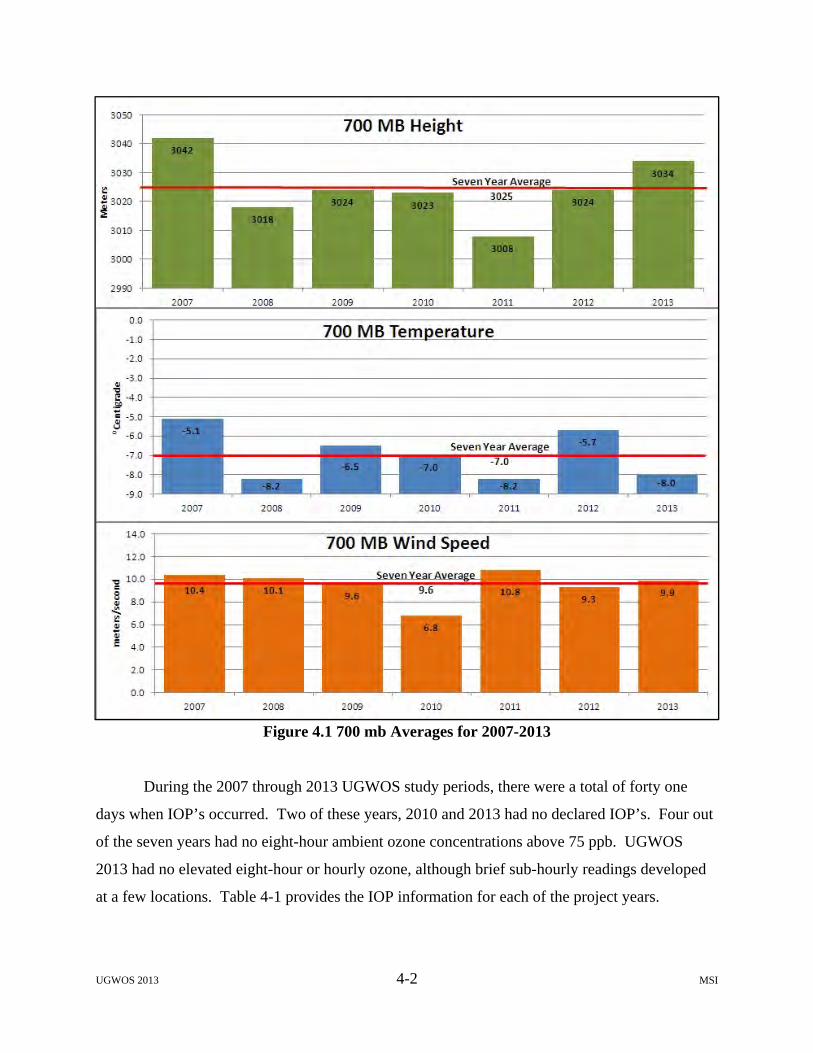
UGWOS 2013 4-2 MSI
Figure 4.1 700 mb Averages for 2007-2013
During the 2007 through 2013 UGWOS study periods, there were a total of forty one
days when IOP’s occurred. Two of these years, 2010 and 2013 had no declared IOP’s. Four out
of the seven years had no eight-hour ambient ozone concentrations above 75 ppb. UGWOS
2013 had no elevated eight-hour or hourly ozone, although brief sub-hourly readings developed
at a few locations. Table 4-1 provides the IOP information for each of the project years.

UGWOS 2013 4-3 MSI
Table 4-1
Intensive Operational Periods by Year
Year Number of
IOP’s Number of IOP
Days Number of Sites
with 8-hour Ozone > 75 ppb
IOP dates
2007 1 6 0 March 14-19
2008 3 10 5
February 18 - 21 February 27 - 29 March 10 - 12
2009 3 9 0 February 3 - 5 February 21 - 22 February 28 – March 3
2010 0 0 0 --
2011 2 7 7 February 28 – March 2 March 9 - 12
2012 6 9 0
January 29 February 5-6 February 16 February 27 March 4-5 March 8-9
2013 0 0 0 -- Total 15 41 -- --
Using reanalysis data2 and incorporating only IOP days over the last seven years yielded
an average 700 mb height of 3071 mb, an average 700 mb temperature of -5.8°C, and an average
700 mb wind speed of 8.1 mps.
For 2013, WDEQ did designate days when VOC canister sampling was to occur. VOC
samples were collected on January 19 and 20, February 3, March 14, and March 28. These days
were designated when high pressure, light winds and sunny skies were expected. Unlike IOP
days, the formation of elevated ozone was not required. Reanalysis data were used to calculate
averaged 700 mb criteria parameters for the 2013 designated VOC sampling days. Over the five
VOC canister sampling days, the average 700 mb height was 3112 meters, the average 700 mb
temperature was -2.1⁰C, and the average 700 mb wind speed was 7.5 mps.
2 http://www.esrl.noaa.gov/psd/cgi-bin/data/composites/printpage.pl. Accessed July 1, 2013.
UGWOS 2013 4-4 MSI
4.1.2 UGWOS Snow Cover in 2012 and 2013
Snow cover is one of the more important elements in developing conditions which favor
elevated ozone in the UGRB during the late winter and early spring months. Although 2013
started out with several inches of snow cover, the weather pattern was active enough that strong
high pressure did not remain in place. This weather pattern did not allow stagnant conditions to
develop over a long enough period of time to accumulate, contain and concentrate the precursors
necessary for ozone development. A similar situation occurred in 2012 which also had a
significant snow cover in place, and elevated ozone failed to develop during that study period as
well.
Due to the lack of measured snow depth information for the UGRB, previous UGWOS
reports provided a comparison of estimated snow depths between the current report year and the
previous years using data provided by NOAA’s National Operational Hydrologic Remote
Sensing Center (NOHRSC) web site3. In 2012, both NOHRSC data and the snow stick images
were used to estimate snow depths and the datasets agreed fairly well.
During the course of the 2013 study it was apparent that snow depth data on the
NOHRSC web site was overestimating actual snow depth based on snow stick imagery. This
overestimation was considerable which would make the 2013 NOHRSC data suspect. Prior to
2012, snow stick information was not available and, therefore, judgments cannot be made as to
whether the NOHRSC estimates were biased in other years as well.
In light of the bias in the NOHRSC data for 2013, a comparison of snow depth was made
using the snow stick images from 2012.
3 http://www.nohrsc.noaa.gov/interactive NOHRSC Interactive Snow Information data provided by NOAA/NWS, Chanhassen, MN, USA, Accessed Jan-May 2013.
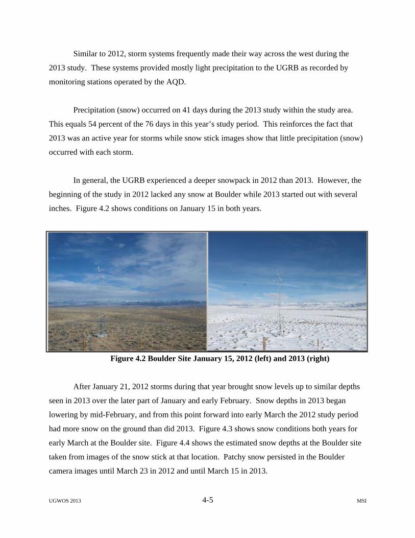
UGWOS 2013 4-5 MSI
Similar to 2012, storm systems frequently made their way across the west during the
2013 study. These systems provided mostly light precipitation to the UGRB as recorded by
monitoring stations operated by the AQD.
Precipitation (snow) occurred on 41 days during the 2013 study within the study area.
This equals 54 percent of the 76 days in this year’s study period. This reinforces the fact that
2013 was an active year for storms while snow stick images show that little precipitation (snow)
occurred with each storm.
In general, the UGRB experienced a deeper snowpack in 2012 than 2013. However, the
beginning of the study in 2012 lacked any snow at Boulder while 2013 started out with several
inches. Figure 4.2 shows conditions on January 15 in both years.
Figure 4.2 Boulder Site January 15, 2012 (left) and 2013 (right)
After January 21, 2012 storms during that year brought snow levels up to similar depths
seen in 2013 over the later part of January and early February. Snow depths in 2013 began
lowering by mid-February, and from this point forward into early March the 2012 study period
had more snow on the ground than did 2013. Figure 4.3 shows snow conditions both years for
early March at the Boulder site. Figure 4.4 shows the estimated snow depths at the Boulder site
taken from images of the snow stick at that location. Patchy snow persisted in the Boulder
camera images until March 23 in 2012 and until March 15 in 2013.

UGWOS 2013 4-6 MSI
Figure 4.3 Boulder Site March 2, 2012 (left) and 2013 (right)
Figure 4.4 Estimated Snow Depth at Boulder Based on Snow Stick Images
4.2 Ozone Spatial and Temporal Distribution
Ozone levels measured during the UGWOS 2013 campaign were fairly low. The highest
8-hour ozone concentration recorded was 64 ppb, which is below the US EPA NAAQS of 75
ppb, and was recorded at only one site on one day. The second highest 8-hour ozone
concentration recorded was 57 ppb. The maximum eight-hour and one-hour ozone
concentrations at all UGWOS 2013 monitoring sites are presented in Figure 4.5.
0.0
5.0
6.0 6.0
0.0 0.0
5.0 5.0
3.0
0.0 0.0 0.00
1
2
3
4
5
6
7
Jan 15 Jan 31 Feb 15 Feb 28 Mar 15 Mar 31
Inches
Date
Snow Depth Estimates
2012
2013
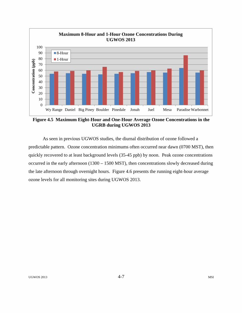
UGWOS 2013 4-7 MSI
Figure 4.5 Maximum Eight-Hour and One-Hour Average Ozone Concentrations in the
UGRB during UGWOS 2013
As seen in previous UGWOS studies, the diurnal distribution of ozone followed a
predictable pattern. Ozone concentration minimums often occurred near dawn (0700 MST), then
quickly recovered to at least background levels (35-45 ppb) by noon. Peak ozone concentrations
occurred in the early afternoon (1300 – 1500 MST), then concentrations slowly decreased during
the late afternoon through overnight hours. Figure 4.6 presents the running eight-hour average
ozone levels for all monitoring sites during UGWOS 2013.
0
10
20
30
40
50
60
70
80
90
100
Wy Range Daniel Big Piney Boulder Pinedale Jonah Juel Mesa Paradise Warbonnet
Con
cen
trat
ion
(p
pb
)Maximum 8-Hour and 1-Hour Ozone Concentrations During
UGWOS 2013
8-Hour
1-Hour
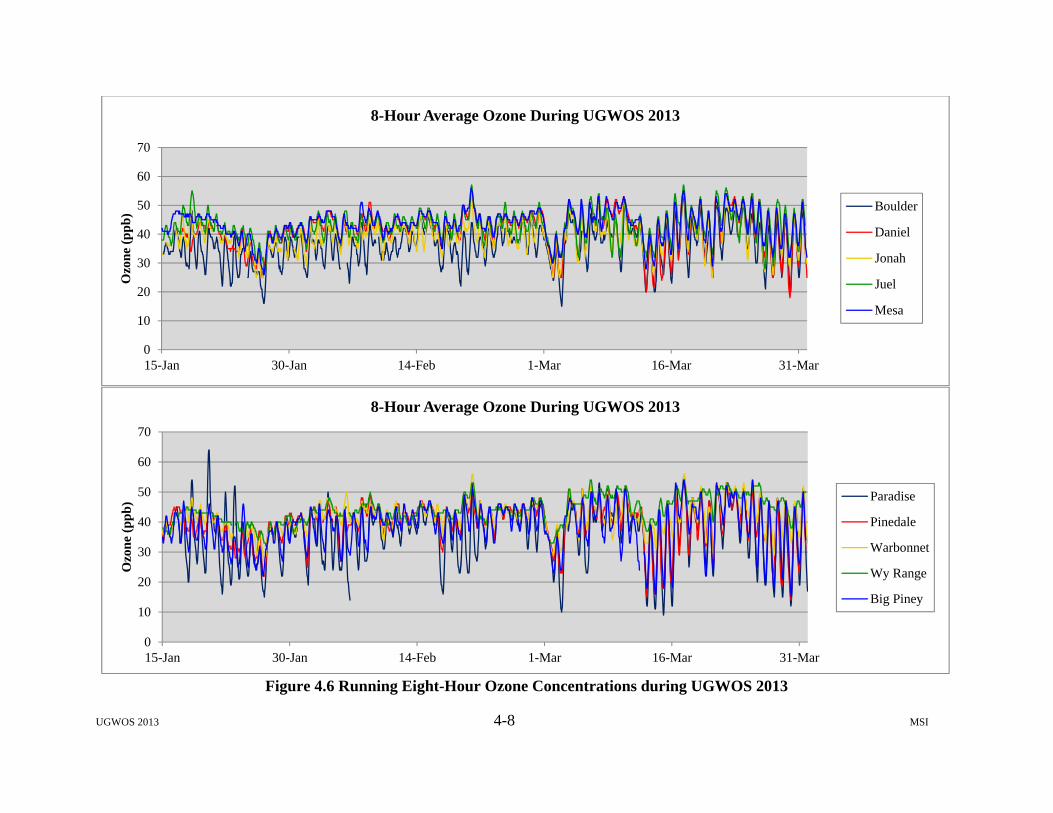
UGWOS 2013 4-8 MSI
Figure 4.6 Running Eight-Hour Ozone Concentrations during UGWOS 2013
0
10
20
30
40
50
60
70
15-Jan 30-Jan 14-Feb 1-Mar 16-Mar 31-Mar
Ozo
ne
(pp
b)
8-Hour Average Ozone During UGWOS 2013
Boulder
Daniel
Jonah
Juel
Mesa
0
10
20
30
40
50
60
70
15-Jan 30-Jan 14-Feb 1-Mar 16-Mar 31-Mar
Ozo
ne
(pp
b)
8-Hour Average Ozone During UGWOS 2013
Paradise
Pinedale
Warbonnet
Wy Range
Big Piney

UGWOS 2013 4-9 MSI
Ozone concentration afternoon maximums occurred most frequently at Juel and Mesa
while ozone concentration morning minimums occurred at Paradise, Big Piney and occasionally
at Pinedale and Boulder. NOx scavenging may contribute to the suppressed morning ozone
minimum concentrations at those sites. As seen in previous years, there was an increase in the
magnitude of the diurnal ozone cycle around the first week of March, coincident with warmer
temperatures and higher sun angles. Looking at the entire study period, ozone concentrations at
all the monitoring sites generally rose and fell together as large-scale weather systems moved
through the UGRB.
Figure 4.7 presents the daily maximum eight-hour average ozone concentrations for all
sites during UGWOS 2013. Juel Springs and/or Mesa experienced the highest ozone
concentrations 81 percent of the time.
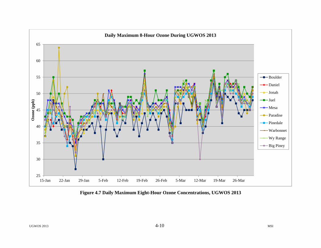
UGWOS 2013 4-10 MSI
Figure 4.7 Daily Maximum Eight-Hour Ozone Concentrations, UGWOS 2013
25
30
35
40
45
50
55
60
65
15-Jan 22-Jan 29-Jan 5-Feb 12-Feb 19-Feb 26-Feb 5-Mar 12-Mar 19-Mar 26-Mar
Ozo
ne
(pp
b)
Daily Maximum 8-Hour Ozone During UGWOS 2013
Boulder
Daniel
Jonah
Juel
Mesa
Paradise
Pinedale
Warbonnet
Wy Range
Big Piney
UGWOS 2013 4-11 MSI
Table 4-2 presents maximum eight-hour average ozone concentrations on any day where
it exceeded 55 ppb at any site in the UGRB. The UGRB network daily maximum is indicated in
the right-most column of the table. Table 4-2 shows that elevated ozone was most commonly
observed at Juel Springs and Warbonnet.
Table 4-2
Maximum Eight-hour Average Ozone Concentrations (ppb) for Boulder (BD), Daniel (DN),
Jonah, Juel Springs, Mesa, Pinedale (PD), Warbonnet (WB), Wyoming Range (WR), and
Big Piney (BP) on Days When at Least One Site Recorded Concentrations > 55 ppb
Station BD DN Jonah Juel
Springs Mesa Paradise PD WB WR BP
Network Max
Jan 20 42 44 45 50 47 64 44 45 43 46 64 Feb 20 44 53 54 57 56 53 50 56 53 51 57 Mar 17 53 55 55 57 55 55 54 56 54 54 57 Mar 22 49 54 54 56 54 53 53 53 53 52 56 Values > 55 in Yellow Values > 60 in Red
4.2.1 Discussion of Spatial and Temporal Distribution of O3 during Designated
VOC Canister Sampling Periods
There were four designated VOC canister sampling periods during UGWOS 2013:
January 19 to January 20, February 3, March 14, and March 28. VOC canister samples were
taken at each mesonet site (Mesa, Warbonnet, and Paradise), at the Jonah Field site and at each
of the following long-term monitoring sites: Boulder, Juel Springs, and Big Piney. An additional
VOC canister was placed a short distance away from the Jonah site to minimize the impact of
local activity on the sample located immediately at the Jonah shelter. Thus, there were a total of
eight distinct VOC canister sites. This section will focus on the spatial and temporal distribution
of ozone in the UGRB during each VOC canister sampling period.
UGWOS 2013 4-12 MSI
The first designated VOC canister sampling period occurred January 19 to January 20.
With the exception of the Paradise site, hourly ozone concentrations on both days remained
below 55 ppb. On January 20, the hourly ozone concentration at the Paradise site reached 86
ppb, but was not elevated long enough to exceed the 8-hour NAAQS of 75 ppb. Ozone
concentrations at the Juel Springs site were also slightly elevated on January 20. During
overnight hours, several sites including Paradise, Boulder, and Big Piney experienced depressed
ozone concentrations to varying degrees likely due to NOx scavenging. Ozone concentrations at
higher elevation sites such as Mesa and Wyoming Range were not depressed during the
overnight hours. The hourly ozone concentrations for January 19 and January 20 are presented
in Figure 4.8.
The second designated VOC canister sampling period was February 3. With the
exception of the Paradise site, hourly ozone concentrations remained at or below 51 ppb. The
Paradise site recorded a one-hour maximum ozone concentration of 65 ppb at 13:00. As with the
first sample period, depressed nocturnal ozone values were observed at Paradise, Boulder, and
Big Piney while little to no nocturnal depression of ozone concentrations was observed at Mesa
and Wyoming Range. The hourly ozone concentrations for February 3 are presented in Figure
4.9.

UGWOS 2013 4-13 MSI
Figure 4.8 One-Hour Average Ozone during Designated VOC Sampling Period 1
Figure 4.9 One-Hour Average Ozone during Designated VOC Sampling Period 2
0
10
20
30
40
50
60
70
80
90
100
0 2 4 6 8 10 12 14 16 18 20 22 0 2 4 6 8 10 12 14 16 18 20 22
Ozo
ne
(pp
b)
Hour of Day (MST)
Hourly Ozone on January 19 - 20, 2013
Boulder
Daniel
Jonah
Juel
Mesa
Paradise
Pinedale
Warbonnet
WyRange
BigPiney
0
10
20
30
40
50
60
70
0 1 2 3 4 5 6 7 8 9 10 11 12 13 14 15 16 17 18 19 20 21 22 23
Ozo
ne
(pp
b)
Hour of Day (MST)
Hourly Ozone on February 3, 2013
Boulder
Daniel
Jonah
Juel
Mesa
Paradise
Pinedale
Warbonnet
WyRange
BigPiney
UGWOS 2013 4-14 MSI
The third and fourth designated VOC sampling periods occurred on March 14 and March
28, respectively. Hourly ozone concentrations on March 14 did not exceed 50 ppb while ozone
concentrations on March 28 did not exceed 54 ppb. Juel Springs was consistently among the
sites with the highest daytime ozone concentrations during these two periods. As seen in
previous sampling periods, NOx scavenging appears to negatively affect ozone concentrations at
low-elevation sites such as Paradise, Boulder, and Big Piney during the overnight hours while
this effect is minimized at sites with higher elevation. The hourly ozone concentrations for
March 14 and March 28 are presented in Figure 4.10 and Figure 4.11, respectively.
In conclusion, the Paradise site was the only site that demonstrated elevated ozone
concentrations during any of the designated VOC sampling periods. Ozone concentrations at the
Juel Springs site, although not elevated, were consistently among the highest of the remainder of
the group. Nocturnal NOx scavenging was evident during each of the sample periods and seems
to have the greatest impact on sites that are low in elevation and close to NOx sources.
Figure 4.10 One-Hour Average Ozone during Designated VOC Sampling Period 3
0
10
20
30
40
50
60
0 1 2 3 4 5 6 7 8 9 10 11 12 13 14 15 16 17 18 19 20 21 22 23
Ozo
ne
(pp
b)
Hour of Day (MST)
Hourly Ozone on March 14, 2013
Boulder
Daniel
Jonah
Juel
Mesa
Paradise
Pinedale
Warbonnet
WyRange
BigPiney

UGWOS 2013 4-15 MSI
Figure 4.11 One-Hour Average Ozone during Designated VOC Sampling Period 4
4.2.2 Surface Wind Patterns Affiliated with Elevated Ozone during Designated
VOC Sampling Periods
There were four VOC sampling periods during UGWOS 2013. This section will focus
on the wind patterns that occurred at sites that observed elevated ozone during these periods. For
this year’s campaign, Paradise and possibly Juel Springs were the only sites where the above
statement holds true. Moreover, since there was no elevated ozone observed during the third and
fourth sampling periods, only the first and second periods will be discussed. For each of these
cases, the hourly average wind (represented by wind barbs) is superimposed upon a line plot of
hourly ozone concentrations. Wind barbs point in the direction from which wind is blowing.
Since observed wind speeds during the sampling periods are usually low, a full barb will
represent a wind speed of 5 mps.
0
10
20
30
40
50
60
0 1 2 3 4 5 6 7 8 9 10 11 12 13 14 15 16 17 18 19 20 21 22 23
Ozo
ne
(pp
b)
Hour of Day (MST)
Hourly Ozone on March 28, 2013
Boulder
Daniel
Jonah
Juel
Mesa
Paradise
Pinedale
Warbonnet
WyRange
BigPiney
UGWOS 2013 4-16 MSI
Paradise was the only site that observed one-hour ozone concentrations in excess of 60
ppb during sampling period 1, specifically on January 20. Ozone concentrations at the Juel
Springs site were also slightly elevated relative to the remainder of the sites in the UGRB.
Hourly wind and ozone for Paradise and Juel Springs during sampling period 1 are represented
in Figure 4.12. Winds at the Paradise site were southerly, except for a shift to the southwest
during the afternoon of both days of sampling period 1. Ozone concentrations build prior to the
wind shift and the wind shift corresponds to the beginning of the decline in ozone concentrations.
Winds at the Juel Springs site are generally northwesterly, except for a shift to westerly or
southwesterly during the afternoon hours of both days of sampling period 1.
Figure 4.12 One-Hour Average Ozone and Wind at Paradise and Juel Springs
during VOC Sampling Period 1
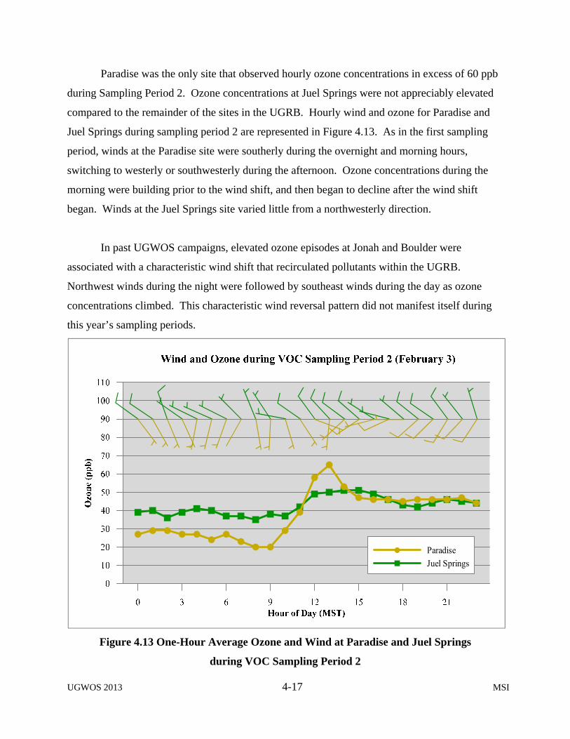
UGWOS 2013 4-17 MSI
Paradise was the only site that observed hourly ozone concentrations in excess of 60 ppb
during Sampling Period 2. Ozone concentrations at Juel Springs were not appreciably elevated
compared to the remainder of the sites in the UGRB. Hourly wind and ozone for Paradise and
Juel Springs during sampling period 2 are represented in Figure 4.13. As in the first sampling
period, winds at the Paradise site were southerly during the overnight and morning hours,
switching to westerly or southwesterly during the afternoon. Ozone concentrations during the
morning were building prior to the wind shift, and then began to decline after the wind shift
began. Winds at the Juel Springs site varied little from a northwesterly direction.
In past UGWOS campaigns, elevated ozone episodes at Jonah and Boulder were
associated with a characteristic wind shift that recirculated pollutants within the UGRB.
Northwest winds during the night were followed by southeast winds during the day as ozone
concentrations climbed. This characteristic wind reversal pattern did not manifest itself during
this year’s sampling periods.
Figure 4.13 One-Hour Average Ozone and Wind at Paradise and Juel Springs
during VOC Sampling Period 2

UGWOS 2013 4-18 MSI
4.2.3 Comparison of Ozone in 2013 with 2005-2012
Ozone data have been recorded at long-term monitoring sites in the UGRB since 2005.
The Jonah, Boulder (BD), Daniel (DN), Pinedale (PD), Juel Springs, and Wyoming Range (WR)
sites utilize Federal Equivalent Method (FEM) air quality monitors. After the conclusion of the
2009 UGWOS campaign, the monitoring equipment at Jonah was dismantled and moved to its
current location at Juel Springs. For the 2010 UGWOS campaign, the WDEQ BAM trailer with
FEM analyzers was placed at the former Jonah long-term site. For the 2012 UGWOS campaign,
power was not available at the former long-term site. Therefore, the WDEQ BAM trailer was
located at the entrance to the Jonah field on the Luman Road, 10.4 kilometers northeast of the
former long-term site. For this year’s UGWOS campaign, the WDEQ BAM trailer was located
inside the Jonah field, 6.2 kilometers northeast of the former long-term site, where a source of
power was available. Eight-hour ozone averages and maxima by month from these sites are
presented in Table 4-3.

UGWOS 2013 4-19 MSI
Table 4-3
Eight-Hour Monthly Average and Maximum Ozone by Year for
Jonah, Boulder, Daniel, Pinedale, Juel Springs, and Wyoming Range
January Average
8-Hour Ozone (ppb) Maximum
8-Hour Ozone (ppb) Year Jonah BD DN PD Juel WR Jonah BD DN PD Juel WR 2005 35 NA NA NA NA NA 78 NA NA NA NA NA 2006 33 41 43 NA NA NA 49 67 53 NA NA NA 2007 27 43 40 NA NA NA 57 71 53 NA NA NA 2008 29 39 42 NA NA NA 47 58 56 NA NA NA 2009 24 34 37 NA 38* NA 52 55 48 NA 64* NA 2010 34† 38 39 36 40 NA 57† 69 49 61 55 NA 2011 NA 39 41 40 42 45 NA 69 59 62 63 54 2012 34† 34 35 33 35 30 47† 52 43 42 50 36 2013 37† 32 39 37 41 40 49† 48 50 46 55 51
February Average 8-Hour Ozone (ppb) Maximum 8-Hour Ozone (ppb) Year Jonah BD DN PD Juel WR Jonah BD DN PD Juel WR 2005 42 51 NA NA NA NA 98 89 NA NA NA NA 2006 39 48 49 NA NA NA 93 71 82 NA NA NA 2007 29 42 40 NA NA NA 46 59 57 NA NA NA 2008 40 54 50 NA NA NA 102 122 76 NA NA NA 2009 33 42 43 NA 40* NA 69 67 64 NA 62* NA 2010 44† 51 46 42 46 NA 54† 62 52 57 53 NA 2011 NA 46 47 44 47 51 NA 87 74 59 68 80 2012 38† 40 40 38 41 39 50† 64 54 50 53 52 2013 40† 37 44 42 43 44 54† 46 53 50 57 53
March Average 8-Hour Ozone (ppb) Maximum 8-Hour Ozone (ppb) Year Jonah BD DN PD Juel WR Jonah BD DN PD Juel WR 2005 40 48 NA NA NA NA 58 71 NA NA NA NA 2006 44 48 50 NA NA NA 68 67 71 NA NA NA 2007 32 44 40 NA NA NA 44 65 55 NA NA NA 2008 39 53 50 NA NA NA 98 102 75 NA NA NA 2009 39 46 43 NA 42* NA 63 70 67 NA 67* NA 2010 48† 53 48 41 49 NA 55† 66 54 57 53 NA 2011 NA 54 52 51 53 55 NA 123 85 89 94 83 2012 42† 41 39 39 43 40 61† 62 58 59 56 50 2013 40† 37 41 39 43 47 55† 53 55 54 57 54
* Temporary Mesonet site with 2B ozone analyzer prior to long-term site. † WDEQ trailer with FEM monitor after long-term site equipment moved to Juel Springs January 15-31 NA – Data not available

UGWOS 2013 4-20 MSI
Monthly average 8-hour ozone concentrations were generally below average during the
2013 UGWOS campaign. Similarly, maximum eight-hour ozone concentrations were low
compared to those of previous years. The highest 8-hour ozone concentration recorded at the
long-term monitoring sites with FEM analyzers was 57 ppb observed at Juel Springs.
4.2.4 Comparison of NOx and PM during UGWOS 2013 with 2006-2012
Average monthly NO and NO2 concentrations at AQD monitoring sites in the UGRB are
presented in Table 4-4. During 2013, concentrations were low with no sites exceeding a monthly
average of 1.4 ppb NO and 6.2 ppb NO2, respectively.

UGWOS 2013 4-21 MSI
Table 4-4
Monthly Average One-Hour NO and NO2 Concentrations by Year for
Jonah, Boulder, Daniel, Pinedale, Juel Springs, and Wyoming Range
Jan. 1-Hour NO (ppb) 1-Hour NO2 (ppb) Year Jonah BD DN PD Juel WR Jonah BD DN PD Juel WR 2006 11.2 1.7 0.04 NA NA NA 16.9 7.2 0.5 NA NA NA 2007 24.6 0.9 0.05 NA NA NA 22.6 4.5 0.7 NA NA NA 2008 27.2 NA 0.01 NA NA NA 26.2 NA 0.2 NA NA NA 2009 20.6 2.5 0.01 NA NA NA 24.4 5.6 0.2 NA NA NA 2010 4.9*† 2.1 NA 0.8 1.3 NA 11.2*† 8.0 0.7 4.3 2.9 NA 2011 NA 1.7 0.02 1.6 0.6 0.1 NA 7.0 0.1 3.9 3.3 0.3 2012 1.3*† 0.4 0.00 1.0 0.2 0.0 3.3*† 2.2 0.0 4.1 0.3 0.5 2013 1.4*† 0.5 NA 0.8 0.3 0.0 3.6*† 6.2 NA 2.1 2.1 0.5 Feb. 1-Hour NO (ppb) 1-Hour NO2 (ppb) Year Jonah BD DN PD Juel WR Jonah BD DN PD Juel WR 2006 16.3 0.9 0.04 NA NA NA 18.1 4.8 0.7 NA NA NA 2007 19.6 0.4 0.01 NA NA NA 16.8 1.7 0.1 NA NA NA 2008 24.0 NA 0.00 NA NA NA 19.0 NA 0.1 NA NA NA 2009 10.6 1.9 0.00 NA NA NA 16.2 5.7 0.4 NA NA NA 2010 8.1† 1.3 NA 0.4 1.3 NA 10.4† 4.6 0.3 2.6 2.9 NA 2011 NA 0.8 0.02 1.8 0.5 0.1 NA 4.8 0.6 5.5 2.5 1.0 2012 0.7† 0.6 0.04 1.2 0.1 0.0 2.5† 2.6 0.0 4.1 0.9 0.6 2013 0.5† 0.2 0.07 0.3 0.2 0.0 2.2† 2.5 0.1 1.5 1.5 0.6 Mar. 1-Hour NO (ppb) 1-Hour NO2 (ppb) Year Jonah BD DN PD Juel WR Jonah BD DN PD Juel WR 2006 0.3 0.01 4.4 NA NA NA 9.0 1.8 0.4 NA NA NA 2007 0.2 0.00 20.3 NA NA NA 16.1 0.7 0.05 NA NA NA 2008 0.03 0.00 13.1 NA NA NA 14.6 0.9 0.02 NA NA NA 2009 0.3 0.00 2.6 NA NA NA 6.9 2.0 0.2 NA NA NA 2010 0.2† NA 7.0 0.9 1.3 NA 6.6† 1.7 0.4 1.9 1.2 NA 2011 0.9 0.00 NA 2.4 0.4 0.1 NA 4.9 0.5 7.4 2.5 0.8 2012 -0.4† 0.1 0.00 1.3 0.1 0.0 0.8† 0.4 0.0 4.3 1.1 0.9 2013 0.1† 0.1 0.09 0.1 0.1 0.0 1.3† 1.5 0.1 1.4 1.0 0.6 * January 15-31 † WDEQ trailer with FEM monitor after long-term site equipment moved to Juel Springs NA – Data not available

UGWOS 2013 4-22 MSI
Average monthly PM10 and PM2.5 concentrations at AQD monitoring sites in the UGRB
are presented in Table 4-5. Monthly average concentrations during 2013 were generally lower
than those from prior years.
Table 4-5
Monthly Average PM10 and PM2.5 Concentrations by Year for
Boulder, Daniel, Pinedale, and Wyoming Range
January Average PM10 (µg/m3) Average PM2.5 (µg/m3) Year Boulder Daniel Wyoming Range Pinedale Wyoming Range 2006 7.1 5.0 NA NA NA 2007 NA 5.2 NA NA NA 2008 6.9 6.4 NA NA NA 2009 6.7 4.9 NA 4.1 NA 2010 6.7 4.3 NA 4.1* NA 2011 6.7 4.4 1.6 4.4 0.8 2012 5.7 4.6 3.7 5.1 0.5 2013 5.5 5.7 1.2 5.3 0.9
February Average PM10 (µg/m3) Average PM2.5 (µg/m3) Year Boulder Daniel Wyoming Range Pinedale Wyoming Range 2006 7.4 6.1 NA NA NA 2007 5.0 4.8 NA NA NA 2008 7.4 5.7 NA NA NA 2009 6.9 6.6 NA 3.6 NA 2010 6.3 4.4 NA 2.4 NA 2011 10.3 6.4 4.4 5.1 2.1 2012 6.0 4.5 3.6 4.8 1.2 2013 4.7 4.0 1.8 2.6 1.0
March Average PM10 (µg/m3) Average PM2.5 (µg/m3) Year Boulder Daniel Wyoming Range Pinedale Wyoming Range 2006 7.7 6.8 NA NA NA 2007 8.5 6.7 NA NA NA 2008 7.5 6.7 NA NA NA 2009 10.9 11.2 NA 4.3 NA 2010 8.2 6.6 NA 3.0 NA 2011 11.1 7.3† 5.7 5.5 3.1 2012 10.0 9.4 8.4 7.0 2.7 2013 7.6 7.1 7.5 3.0 1.5
* January 15-31, 2010. † March 1-20, 2011. NA – Data not available
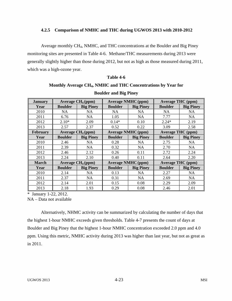
UGWOS 2013 4-23 MSI
4.2.5 Comparison of NMHC and THC during UGWOS 2013 with 2010-2012
Average monthly CH4, NMHC, and THC concentrations at the Boulder and Big Piney
monitoring sites are presented in Table 4-6. Methane/THC measurements during 2013 were
generally slightly higher than those during 2012, but not as high as those measured during 2011,
which was a high-ozone year.
Table 4-6
Monthly Average CH4, NMHC and THC Concentrations by Year for
Boulder and Big Piney
January Average CH4 (ppm) Average NMHC (ppm) Average THC (ppm) Year Boulder Big Piney Boulder Big Piney Boulder Big Piney 2010 NA NA NA NA NA NA 2011 6.76 NA 1.05 NA 7.77 NA 2012 2.10* 2.09 0.14* 0.10 2.24* 2.19 2013 2.57 2.37 0.52 0.22 3.09 2.58
February Average CH4 (ppm) Average NMHC (ppm) Average THC (ppm) Year Boulder Big Piney Boulder Big Piney Boulder Big Piney 2010 2.46 NA 0.28 NA 2.75 NA 2011 2.39 NA 0.32 NA 2.70 NA 2012 2.46 2.12 0.26 0.11 2.72 2.24 2013 2.24 2.10 0.40 0.11 2.64 2.20
March Average CH4 (ppm) Average NMHC (ppm) Average THC (ppm) Year Boulder Big Piney Boulder Big Piney Boulder Big Piney 2010 2.14 NA 0.13 NA 2.27 NA 2011 2.37 NA 0.31 NA 2.69 NA 2012 2.14 2.01 0.15 0.08 2.29 2.09 2013 2.18 1.93 0.29 0.08 2.46 2.01
* January 1-22, 2012. NA – Data not available
Alternatively, NHMC activity can be summarized by calculating the number of days that
the highest 1-hour NMHC exceeds given thresholds. Table 4-7 presents the count of days at
Boulder and Big Piney that the highest 1-hour NMHC concentration exceeded 2.0 ppm and 4.0
ppm. Using this metric, NMHC activity during 2013 was higher than last year, but not as great as
in 2011.

UGWOS 2013 4-24 MSI
Table 4-7
Number of Days That Highest 1-Hr NMHC Concentration
Exceeded 2.0 ppm and 4.0 ppm at Boulder and Big Piney
Boulder Big Piney Year Days > 2 ppm Days > 4 ppm Days > 2 ppm Days > 4 ppm 2010 1 0 NA NA 2011 16 3 NA NA 2012 0 0 0 0 2013 4 1 0 0
For each day during UGWOS 2013, the maximum 8-hour ozone concentration and
average NMHC concentration were calculated at the Boulder and Big Piney sites. These data are
presented as scatter plots in Figure 4.14 for Boulder and Figure 4.15 for Big Piney along with
similar data from previous years.
Figure 4.14 Comparison of Maximum 8-hour Ozone and Daily Average NMHC at Boulder for UGWOS 2011 – 2013. Linear regression fit for 2013 data is shown.
R² = 0.0561
0
20
40
60
80
100
120
140
0 0.2 0.4 0.6 0.8 1 1.2 1.4 1.6
Ozo
ne
(pp
b)
NMHC (ppm)
Daily Average NMHC and Daily Maximum 8-hr O3 at Boulder, UGWOS 2011 - 2013
2011
2012
2013
2013

UGWOS 2013 4-25 MSI
Figure 4.15 Comparison of Maximum 8-hour Ozone and Daily Average NMHC at Big Piney for UGWOS 2012 – 2013. Linear regression fit for 2013 data is shown.
While it is true that the highest ozone concentration measured in 2011 (123 ppb at
Boulder) occurred on the same day as the highest NMHC concentration (1.1 ppm), there are
several days that year in which NMHC were measured in relatively high concentrations without
high ozone concentrations to match. In 2013, there were many days at Boulder which recorded
levels of NMHC in excess of 0.5 ppm, which is similar to the levels associated with high ozone
days in 2011. However, ozone levels on those days in 2013 were not associated with elevated
ozone concentrations. At Big Piney, there were many days which recorded levels of NMHC
higher than those in 2012 but were not associated with elevated ozone levels. For both sites in
2013, there was no correlation between daily average NMHC concentrations and daily maximum
8-hr ozone concentrations.
R² = 0.0419
0
10
20
30
40
50
60
0 0.1 0.2 0.3 0.4 0.5 0.6 0.7
Ozo
ne
(pp
b)
NMHC (ppm)
Daily Average NMHC and Daily Maximum 8-hr O3 atBig Piney, UGWOS 2012 - 2013
2012
2013
2013

UGWOS 2013 4-26 MSI
4.3 VOC Canister Sampling
The goal of the UGWOS 2013 VOC canister sampling stemmed from the UGWOS 2012
study to investigate the spatial distribution of precursor concentrations in and around the gas and
oil fields located in the UGRB. To obtain a spatial distribution of precursors, VOC canister
samples were collected at Boulder, Juel Springs, and Big Piney monitoring stations as well as the
UGWOS-specific Jonah air quality site and three mesonet sites (Paradise, Mesa, and
Warbonnet). In addition to the sampling at the Jonah site, VOC samples were also collected at a
second Jonah site located 410 meters north-northeast of the air quality site. Although no IOPs
were initiated during the 2013 UGWOS study period, five samples were taken at each station
during periods in which a high pressure system was located over the study area and light winds
were present.
VOC samples were collected using 6-liter SUMMA canisters connected to canister
samplers which were programmed to collect 3-hour samples between the hours of 07:00 and
10:00 MST. Figures 4.16 and 4.17 present a summary of the VOC samples broken into five
categories of hydrocarbons (Paraffins, Isoparaffins, Aromatics, Naphthenes, and Olefins) and
Oxygenates at each of the eight sample locations. Figures 4.18 and 4.19 present the percentage
composition of each hydrocarbon category in the samples. Dates in which samples were taken
are shown on the x-axis and are presented in chronological order to compare site concentrations
throughout the study period.
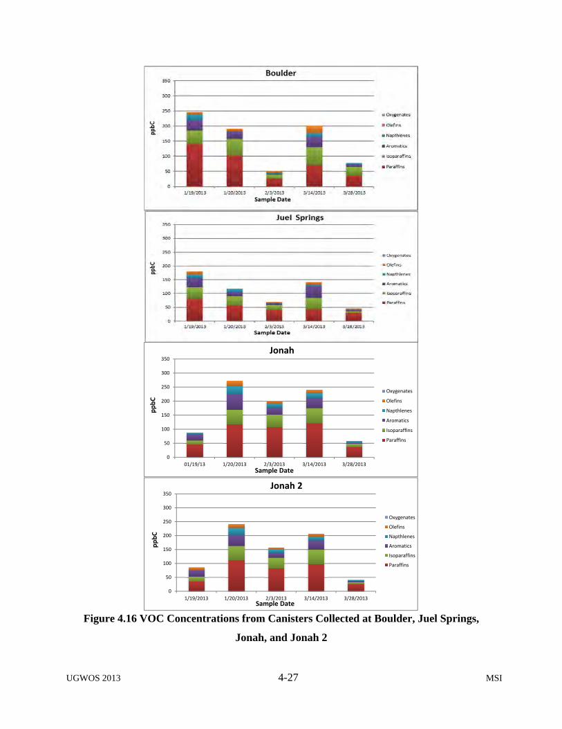
UGWOS 2013 4-27 MSI
Figure 4.16 VOC Concentrations from Canisters Collected at Boulder, Juel Springs,
Jonah, and Jonah 2
0
50
100
150
200
250
300
350
01/19/13 1/20/2013 2/3/2013 3/14/2013 3/28/2013
ppbC
Sample Date
Jonah
Oxygenates
Olefins
Napthlenes
Aromatics
Isoparaffins
Paraffins
0
50
100
150
200
250
300
350
1/19/2013 1/20/2013 2/3/2013 3/14/2013 3/28/2013
ppbC
Sample Date
Jonah 2
Oxygenates
Olefins
Napthlenes
Aromatics
Isoparaffins
Paraffins
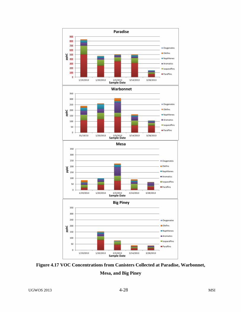
UGWOS 2013 4-28 MSI
Figure 4.17 VOC Concentrations from Canisters Collected at Paradise, Warbonnet,
Mesa, and Big Piney
0
100
200
300
400
500
600
700
800
900
1/19/2013 1/20/2013 2/3/2013 3/14/2013 3/28/2013
ppbC
Sample Date
Paradise
Oxygenates
Olefins
Napthlenes
Aromatics
Isoparaffins
Paraffins
0
50
100
150
200
250
300
350
01/19/13 1/20/2013 2/3/2013 3/14/2013 3/28/2013
ppbC
Sample Date
Warbonnet
Oxygenates
Olefins
Napthlenes
Aromatics
Isoparaffins
Paraffins
0
50
100
150
200
250
300
350
1/19/2013 1/20/2013 2/3/2013 3/14/2013 3/28/2013
ppbC
Sample Date
Mesa
Oxygenates
Olefins
Napthlenes
Aromatics
Isoparaffins
Paraffins
0
50
100
150
200
250
300
350
1/19/2013 1/20/2013 2/3/2013 3/14/2013 3/28/2013
ppbC
Sample Date
Big Piney
Oxygenates
Olefins
Napthlenes
Aromatics
Isoparaffins
Paraffins

UGWOS 2013 4-29 MSI
Figure 4.18 Relative Composition from Canisters Collected at Boulder, Juel Springs,
Jonah, and Jonah 2
0%
10%
20%
30%
40%
50%
60%
70%
80%
90%
100%
1/19/2013 1/20/2013 2/3/2013 3/14/2013 3/28/2013
Relative
Composition
Sample Date
Boulder
Oxygenates
Olefins
Napthlenes
Aromatics
Isoparaffins
Paraffins
0%
10%
20%
30%
40%
50%
60%
70%
80%
90%
100%
01/19/13 1/20/2013 2/3/2013 3/14/2013 3/28/2013
Relative
Composition
Sample Date
Jonah
Oxygenates
Olefins
Napthlenes
Aromatics
Isoparaffins
Paraffins
0%
10%
20%
30%
40%
50%
60%
70%
80%
90%
100%
1/19/2013 1/20/2013 2/3/2013 3/14/2013 3/28/2013
Relative
Composition
Sample Date
Jonah 2
Oxygenates
Olefins
Napthlenes
Aromatics
Isoparaffins
Paraffins

UGWOS 2013 4-30 MSI
Figure 4.19 Relative Composition from Canisters Collected at Paradise, Warbonnet,
Mesa, and Big Piney
0%
10%
20%
30%
40%
50%
60%
70%
80%
90%
100%
1/19/2013 1/20/2013 2/3/2013 3/14/2013 3/28/2013
Relative
Composition
Sample Date
Paradise
Oxygenates
Olefins
Napthlenes
Aromatics
Isoparaffins
Paraffins
0%
10%
20%
30%
40%
50%
60%
70%
80%
90%
100%
01/19/13 1/20/2013 2/3/2013 3/14/2013 3/28/2013
Relative
Compostion
Sample Date
Warbonnet
Oxygenates
Olefins
Napthlenes
Aromatics
Isoparaffins
Paraffins
0%
10%
20%
30%
40%
50%
60%
70%
80%
90%
100%
1/19/2013 1/20/2013 2/3/2013 3/14/2013 3/28/2013
Relative
Composition
Sample Date
Mesa
Oxygenates
Olefins
Napthlenes
Aromatics
Isoparaffins
Paraffins
0%
10%
20%
30%
40%
50%
60%
70%
80%
90%
100%
1/19/2013 1/20/2013 2/3/2013 3/14/2013 3/28/2013
Relative
Composition
Sample Date
Big Piney
Oxygenates
Olefins
Napthlenes
Aromatics
Isoparaffins
Paraffins

UGWOS 2013 4-31 MSI
VOC concentrations at Paradise were consistently higher than the other seven sample
locations. The Paradise mesonet site was located 3.76 miles southwest of the Boulder air quality
site in the heart of the gas and oil operations (primarily well production and liquid gathering
system). The location of the Paradise site also placed it in the low lands adjacent to the New Fork
River flood plain. To some extent, the lower elevation and surrounding terrain sheltered the site
from regional wind patterns leading to lower wind speeds relative to other VOC sample sites.
This is evident when looking at the wind statistics for the eight VOC sampling locations. Lower
wind speeds lead to less dilution and the lower terrain allows for more localized pooling of
VOCs from nearby sources. Table 4-8 presents the maximum and average wind speeds for the
study period and for days in which VOC samples were taken.
Table 4-8
Wind Speed Statistics for VOC Sample Locations
Time Period WS Stat. Boulder Warbonnet Jonah Jonah2 Paradise Mesa Big Piney
Study Period Maximum 20.5 14.01 13.77 14.33 10.16 12.80 13.70 Average 4.24 3.61 3.49 3.73 2.68 3.61 2.44
Sam
ple
Day
s
1/19/2013 Maximum 5.40 3.69 5.73 N/A1 2.40 5.16 3.80 Average 2.39 2.77 3.63 N/A1 0.83 2.68 1.88
1/20/2013 Maximum 8.90 6.33 5.95 N/A1 5.46 6.66 6.10 Average 3.27 2.95 3.65 N/A1 1.73 3.74 1.97
2/03/2013 Maximum 8.40 4.12 4.97 4.80 6.04 5.85 2.70 Average 3.98 2.82 3.55 3.40 2.42 3.58 1.27
3/14/2013 Maximum 5.40 4.40 4.77 4.74 3.44 3.10 5.70 Average 2.89 1.87 2.06 2.31 1.32 1.83 2.37
3/28/2013 Maximum 5.00 4.36 4.62 4.68 3.46 3.43 4.60 Average 3.13 2.33 2.25 2.45 1.71 1.89 1.98
Cumulative Sample Days
Maximum 8.90 6.33 5.95 4.801 6.04 6.66 6.10 Average 3.13 2.55 3.03 2.721 1.60 2.74 1.90
1Jonah 2 wind measurements started on January 29th at 11:00
UGWOS 2013 4-32 MSI
4.3.1 Jonah and Jonah 2
The original Jonah site was removed and access to power was not available at the original
location. The site utilized in 2012 was located on the eastern edge of the Jonah Field. After
investigating several possible alternatives, a site just outside the property line of the Linn Energy
facility was selected as the best alternative since the facility was willing to allow access to their
power. The location is approximately 6 kilometers west of the 2012 site and more representative
of the Jonah Field. Concerns about the effects of regular truck traffic at the Linn Energy facility
on VOC measurements prompted the installation of a control site (Jonah 2) approximately 410
meters north-northeast.
Results of the Jonah and Jonah 2 VOC sampling showed total NMHC concentrations had
good correlation (R2 = 0.9845) with Jonah showing a slightly higher bias than Jonah 2. The
agreement between the two sites shows that the measurements at Jonah are more representative
of a mesoscale measurement and not heavily affected by the truck traffic from the Linn Energy
facility. A windrose was created with sub-hourly wind data for each sample period (07:00 –
10:00) to help determine the origin of the VOC’s. Wind patterns at both Jonah and Jonah 2 had
good agreement though wind data at Jonah 2 did not commence until January 29. Windroses
show the air mass moving predominantly out of the northwest and north-northwest on January
19, 20, and February 3. Winds were light and variable on March 14 and primarily out of the
north on March 28 with light wind speeds. Figure 4.20 presents the results and sample period
windroses from Jonah and Jonah 2.
UGWOS 2013 4-33 MSI
Figure 4.20 Total NMHC and Sample Time Windroses for Jonah and Jonah 2

UGWOS 2013 4-34 MSI
4.3.2 Comparison of 2013 to 2012 Study
Four locations (Jonah, Juel Springs, Big Piney, and Boulder) collected VOC samples in
both 2012 and 2013. Due to site power availability, the Jonah site is the only site which collected
VOC canister data that has a different location in 2013 from the 2012 study. The location of the
Jonah site in 2013 was approximately 3.75 miles West from the 2012 location. This section
describes the similarities and differences between the 2012 and 2013 studies. The anomalous
VOC concentrations collected on March 8, 2012 at Juel Springs and January 19, 2013 at Big
Piney will be left out of the comparison.
Throughout the UGWOS 2012 study period, eleven samples were collected at each site.
Five samples were collected at each site during 2013 with the exception of Boulder. In addition
to the UGWOS specific VOC sampling system set up at Boulder for the 2013 study, sampling of
ozone precursors is being conducted by an automated system at the Boulder site through the use
of SUMMA canister samples and subsequent laboratory analysis using EPA method TO-14A.
Automated canister samples are initiated when NMHC concentrations on the Baseline-Mocon
9000 analyzer reaches a threshold of two (2) ppm in a five-minute period. Between the
automated canister system and the UGWOS tripod system, the Boulder site collected a total of
fifteen (15) samples during the UGWOS 2013 study period including an unintentional
simultaneous (collocated) sample collected on the morning of January 19, 2013. Figure 4.21
presents a compilation of the Boulder VOC canister data from UGWOS 2012 and 2013.

UGWOS 2013 4-35 MSI
Figure 4.21 Boulder VOC Data from UGWOS 2012 and 2013
Total NMHC concentrations measured via SUMMA canisters at Jonah, Big Piney, and
Juel Springs were slightly higher in 2012 than those measured in 2013. Both years had relatively
low concentrations throughout the study period when compared to canister data from the 2011
study. In 2011, during periods with high ozone concentrations, 12 canisters were collected by a
tethered balloon near the 2013 Paradise location and grab sample concentrations of Total NMHC
ranged from 625 ppbC to 7365 ppbC with an average concentration of 2569 ppbC. Maximum 3-
hour sample concentrations of Total NMHC for Jonah, Juel Springs, and Big Piney were
between 234 and 288 ppbC in 2012 and between 155 and 273 ppbC for 2013. Average
concentrations of Total NMHC ranged from 78.5 to 128.7 ppbC for 2012 and between 78.7 and
172.7 ppbC for 2013. Of the four stations that were retained for VOC canister samples, Boulder
had the highest concentrations of Total NMHC. For Boulder, maximum concentrations of Total
NMHC from 3-hour canister samples ranged from 93.2 to 825.9 ppbC in 2012 and from 11.4 to
682.6 ppbC in 2013. Boulder is adjacent to the gas and oil operations in the Pinedale Anticline
natural gas production field and is expected to have higher concentrations of Total NMHC when
compared to the other three stations.
0
100
200
300
400
500
600
700
800
900
ppbC
Sample Date
Boulder VOC 2012
Oxygenates
Olefins
Napthlenes
Aromatics
Isoparaffins
Paraffins
0%
10%
20%
30%
40%
50%
60%
70%
80%
90%
100%
Sample Date
Boulder VOC 2012
Oxygenates
Olefins
Napthlenes
Aromatics
Isoparaffins
Paraffins
0
100
200
300
400
500
600
700
800
900
ppbC
Sample Date
Boulder VOC 2013
Oxygenates
Olefins
Napthlenes
Aromatics
Isoparaffins
Paraffins
UGWOS Tripod0%
10%
20%
30%
40%
50%
60%
70%
80%
90%
100%
Sample Date
Boulder VOC 2013
Oxygenates
Olefins
Napthlenes
Aromatics
Isoparaffins
Paraffins+ + + + +
+ UGWOS Tripod

UGWOS 2013 4-36 MSI
Between 2012 and 2013, there is good agreement with the composition of the Total
NMHC concentrations when broken into percent contribution of each classification (Paraffins,
Isoparaffins, Aromatics, Napthlenes, Olefins, and Oxygenates) with paraffins having the greatest
percentage of total composition. Figure 4.22 presents the maximum and average percent
contribution of each composition classification for Boulder.
Figure 4.22 Percent Composition of VOC Classifications
4.3.3 VOC Maximum Incremental Reactivity Analysis
Though the measured Total NMHC was relatively low for both 2012 and 2013, ozone
concentrations measured throughout the basin were also low when compared to previous study
years. Non-methane organic compound species vary greatly in the degree to which they
participate in photochemical reactions. Maximum incremental reactivity (MIR) values (Carter
2009) were used to determine the impacts of available VOCs on the formation of ground level
ozone. Potential ozone formation from VOC concentrations is calculated by multiplying the
compound specific MIR value by the concentration of the corresponding compound. The MIR
enhanced values are summed for a Total NMHC ozone formation potential.
0%
10%
20%
30%
40%
50%
60%
70%
Paraffins (%) Isoparaffins (%) Aromatics (%) Napthlenes (%) Olefins (%) Oxygenates (%)
Percent Composition
Boulder Percent Composition of VOC Clasifications for 2012 and 2013
2012 2013
UGWOS 2013 4-37 MSI
Figure 4.23 presents the relationship of the actual Total NMHC and MIR enhanced Total
NMHC concentrations measured at Boulder. The ratio of the actual Total NMHC and MIR
enhanced NMHC varies from day to day due to specific compounds with high MIR values being
measured in the sample analysis. This led to an analysis to determine which measured
compounds were the most abundant in 2013 based on the potential for ozone formation. Table
4-9 presents the top 15 compounds with the highest average concentrations measured as well as
the top 15 compounds available for ozone formation. It was found that on average throughout the
basin ethane was the most abundant compound measured as well as the most available
compound to produce ozone. In 2013, the number of days with conditions favoring higher
NMHC concentrations was considerably less than in 2011 (see Table 4-7) a year when the
current ozone standard was exceeded on 13 days during the UGWOS 2011 study.
Figure 4.23 Actual and MIR Enhanced Total NMHC
0
200
400
600
800
1000
1200
1400
1600
ppbC
2013 Photolytic Ozone Formation Potential from NMHC (Boulder)
Actual NMHC (ppbC)
MIR*NMHC (ppbC)

UGWOS 2013 4-38 MSI
Table 4-9
Top Compounds by Concentration and Potential Reactivity
Rank Top 15 Compounds by Concentration
Top 15 Compounds by Reactivity (MIR)
1 Ethane Ethane 2 Propane Toluene 3 i-Butane m,p-xylene 4 n-Butane Propane 5 i-Pentane 1-Butene 6 Toluene i-Butane 7 n-Pentane Propene 8 Methylcyclohexane n-Butane 9 Benzene i-Pentane
10 n-Hexane 1,2,4-Trimethylbenzene 11 Acetylene Ethene 12 2,4-Dimethylpentane Methylcyclohexane 13 Cyclohexane o-xylene 14 2-Methylpentane n-Pentane 15 m,p-xylene n-Hexane
4.3.4 VOC Quality Control Results
Throughout the study period, collocated samples were taken to reduce uncertainty in
concentration measurements. A separate tripod containing an identical canister sampler system
was collocated with three different VOC canister sites (Juel Springs, Warbonnet, and Big Piney)
once during the study period. Figures 4.24, 4.25, and 4.26 present summaries of the collocated
sample results collected on February 3 at Juel Springs, March 14 at Warbonnet, and March 28 at
Big Piney. The results of the collocated canisters show differences in Sampled Total NMHC of
6.4%, 18.6%, and 37.5% for Juel Springs, Warbonnet, and Big Piney, respectively. The high
percent differences are a result of low concentrations measured throughout the study period. For
such low concentrations, the agreement between the collocated samples was relatively good and
did not have any major outliers.
UGWOS 2013 4-39 MSI
Figure 4.24 February 3, 2013 Collocated Sample Comparison from Juel Springs
Figure 4.25 March 14, 2013 Collocated Sample Comparison from Warbonnet
0
10
20
30
40
50
60
70
80
02/03/2013 Primary 02/03/2013 Duplicate
ppbC
Sample
Juel Springs Duplicate Comparison (02/03/2013)
Oxygenates
Olefins
Napthlenes
Aromatics
Isoparaffins
Paraffins
0
50
100
150
200
250
03/14/2013 Primary 03/14/2013 Duplicate
ppbC
Sample Date
Warbonnet Duplicate Comparison (03/14/2013)
Oxygenates
Olefins
Napthlenes
Aromatics
Isoparaffins
Paraffins
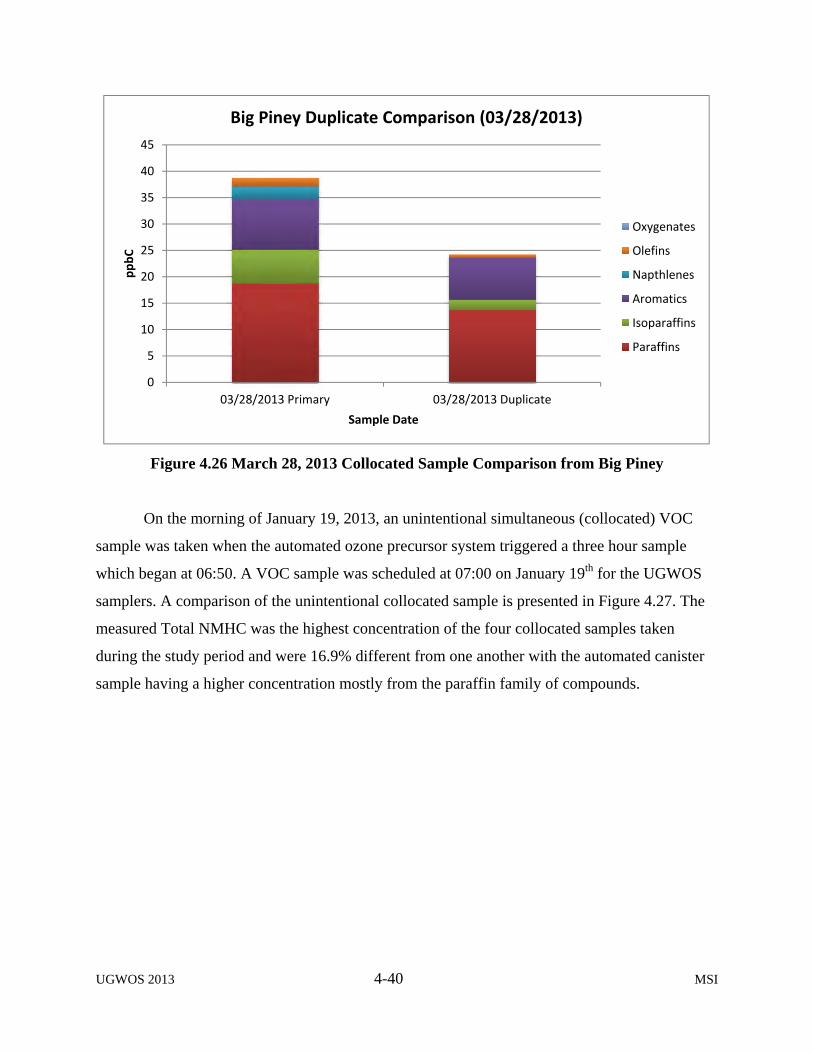
UGWOS 2013 4-40 MSI
Figure 4.26 March 28, 2013 Collocated Sample Comparison from Big Piney
On the morning of January 19, 2013, an unintentional simultaneous (collocated) VOC
sample was taken when the automated ozone precursor system triggered a three hour sample
which began at 06:50. A VOC sample was scheduled at 07:00 on January 19th for the UGWOS
samplers. A comparison of the unintentional collocated sample is presented in Figure 4.27. The
measured Total NMHC was the highest concentration of the four collocated samples taken
during the study period and were 16.9% different from one another with the automated canister
sample having a higher concentration mostly from the paraffin family of compounds.
0
5
10
15
20
25
30
35
40
45
03/28/2013 Primary 03/28/2013 Duplicate
ppbC
Sample Date
Big Piney Duplicate Comparison (03/28/2013)
Oxygenates
Olefins
Napthlenes
Aromatics
Isoparaffins
Paraffins
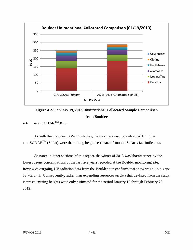
UGWOS 2013 4-41 MSI
Figure 4.27 January 19, 2013 Unintentional Collocated Sample Comparison
from Boulder
4.4 miniSODARTM Data
As with the previous UGWOS studies, the most relevant data obtained from the
miniSODARTM (Sodar) were the mixing heights estimated from the Sodar’s facsimile data.
As noted in other sections of this report, the winter of 2013 was characterized by the
lowest ozone concentrations of the last five years recorded at the Boulder monitoring site.
Review of outgoing UV radiation data from the Boulder site confirms that snow was all but gone
by March 1. Consequently, rather than expending resources on data that deviated from the study
interests, mixing heights were only estimated for the period January 15 through February 28,
2013.
0
50
100
150
200
250
300
350
01/19/2013 Primary 01/19/2013 Automated Sample
ppbC
Sample Date
Boulder Unintentional Collocated Comparison (01/19/2013)
Oxygenates
Olefins
Napthlenes
Aromatics
Isoparaffins
Paraffins

UGWOS 2013 4-42 MSI
Table 4-10 summarizes and compares key mixing height metrics for 2009, 2010, 2012,
and 2013. Metrics were calculated for the period of January 15 through February 28 for each
year from Boulder site data in order to be comparable with the 2013 data. Note that since the
2011 study concentrated on two specific episodes, mixing heights were not estimated for the
entire study period, and 2011 consequently is not included in the table.
Table 4-10
Boulder Mixing Height and Meteorological Metrics – January 15 through February 28
2009 2010 2012 2013 Percentage of hours with reported mixing height (%) 53 56 43 44 Percentage of afternoon hours with reported mixing heights (%) 48 15 21 29 Overall average of reported mixing heights (m) 90* 46 54 48 Days with low mixing heights through afternoon 10 3 4 9 Days with Eight-Hour peak ozone > 60 ppb 4 2 2 0 Days with One-Hour peak ozone > 60 ppb 8 8 12 1 Highest Eight-Hour average ozone (ppb) 69 69 64 53 Average Two-meter temperature (°C) -9.3 -8.6 -10.2 -8.9 Average delta temperature (°C) -0.59 -0.54 0.57 0.15 Average incoming UV radiation, hrs 7 - 17 (W/m2) 20 18.4 18.5 18.6 Average outgoing UV radiation, hrs 7 - 17 (W/m2) 16.9 12.7 15.5 9.7 Total available (incoming + outgoing) UV radiation hrs 7 – 17 (W/m2) 36.9 31.1 34.0 28.3
*Sodar site located at original location at an elevation approximately 50m lower than current site – thus mixing layer heights are similar to other years.
Review of Table 4-9 shows the following:
The percentage of hours during which a measured mixing height was detected is similar
from year-to-year, with the Sodar identifying a defined top to the mixing layer
approximately 50% of the time. 2013 is no exception, though with only 44% of hours, it
was at the low end of the spectrum, equating to a higher percentage of hours when the
near-surface atmosphere was well mixed.

UGWOS 2013 4-43 MSI
In contrast, there is more variability between years in the percentage of hours from noon
to early afternoon period (hours 11 – 15) during which a measured mixing height was
estimated. Relatively stable conditions during this period continue to appear necessary
for the formation of higher ozone concentrations, as noted in previous reports. While the
number of days with peak one-hour average ozone concentrations exceeding 60 ppb is
similar for 2009, 2010, and 2012, the higher frequency of peak eight-hour average
concentrations in 2009 is consistent with somewhat more stable conditions overall
during that year. In contrast, the number of peak one-hour ozone concentrations
exceeding 60 ppb during 2013 is extremely low (only one day), despite having the
second highest percentage of afternoon hours with low mixing heights.
The number of days when mixing heights remained low throughout the afternoon
typically has an indication of overall stability for the winter season. Once again, 2013 is
a bit of an anomaly, with a higher percentage of such days than 2010 and 2012, but
notably lower ozone readings than those recorded during these years. The percentage is
similar to that noted in 2009, which had the most days with the peak eight-hour average
greater than 60 ppb. In contrast, the peak eight-hour average measured at Boulder for
2013 was only 53 ppb.
Thus, 2013 had mixing heights that were similar in many ways with the other three years,
and that actually look slightly more favorable for increased ozone concentrations when compared
with the other three years. Despite this, ozone concentrations measured at the Boulder site
during 2013 were very low – the lowest of any UGWOS year.
UGWOS 2013 4-44 MSI
To investigate possible meteorological differences between the years that would account
for this observation, averages for temperature, delta temperature (inversion strength), and UV
radiation were calculated for each year and are presented in Table 4-9. What immediately stands
out is the significantly lower daily average outgoing UV radiation for 2013 and the total
available (sum of the incoming and outgoing) UV, values that are consistent with the low snow
amounts associated with this year. Previous UGWOS reports have consistently noted the
importance of snow for both increasing the amount of effective UV radiation and maintaining
surface inversions and low mixing layers. The 2013 data implies that of these two issues,
increased UV radiation available for ozone production may be the more critical factor.
Another factor that deserves consideration from the observed data is the lower outgoing,
or reflected UV from the snow cover implies that the surface absorbed the UV and is likely
reradiating the energy in the infrared spectrum. This energy, while no longer in a spectrum that
will enhance ozone production, will likely affect the atmospheric mixing properties by producing
a more thermally turbulent air mass in the mixed layer. This increased thermally induced
turbulence will potentially lower the associated pollutant concentrations through better vertical
mixing within the mixed layer. While not performed as part of this analysis, consideration
should be given to a more detailed analysis of the vertical velocity data from the miniSODAR™
to help understand the role of potentially increased vertical motion. In particular, the vertical
turbulence, as reported by the standard deviation of the vertical wind speed, may shed light on
the mixing associated with the periods of snow cover versus no snow cover.
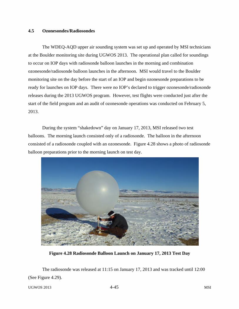
UGWOS 2013 4-45 MSI
4.5 Ozonesondes/Radiosondes
The WDEQ-AQD upper air sounding system was set up and operated by MSI technicians
at the Boulder monitoring site during UGWOS 2013. The operational plan called for soundings
to occur on IOP days with radiosonde balloon launches in the morning and combination
ozonesonde/radiosonde balloon launches in the afternoon. MSI would travel to the Boulder
monitoring site on the day before the start of an IOP and begin ozonesonde preparations to be
ready for launches on IOP days. There were no IOP’s declared to trigger ozonesonde/radiosonde
releases during the 2013 UGWOS program. However, test flights were conducted just after the
start of the field program and an audit of ozonesonde operations was conducted on February 5,
2013.
During the system “shakedown” day on January 17, 2013, MSI released two test
balloons. The morning launch consisted only of a radiosonde. The balloon in the afternoon
consisted of a radiosonde coupled with an ozonesonde. Figure 4.28 shows a photo of radiosonde
balloon preparations prior to the morning launch on test day.
Figure 4.28 Radiosonde Balloon Launch on January 17, 2013 Test Day
The radiosonde was released at 11:15 on January 17, 2013 and was tracked until 12:00
(See Figure 4.29).
UGWOS 2013 4-46 MSI
Figure 4.29 Morning Radiosonde on January 17, 2013 Test Day
The afternoon ozonesonde was collocated with the Boulder monitoring site’s ozone
analyzer sample inlet prior to launch as a quality control check. The Boulder ozone analyzer
indicated an ambient ozone concentration of 45 ppb while the ozonesonde package read 42.3
ppb. The balloon was launched at 15:40 and was tracked until 16:22 (See Figure 4.30).
Figure 4.30 Afternoon Ozonesonde/Radiosonde on January 17, 2013 Test Day

UGWOS 2013 4-47 MSI
On February 5, 2013, an audit was conducted by T&B Systems on the ozonesonde
preparation process. An ozonesonde was prepared completely in a ready to launch status, tested
with a few different known ozone concentration inputs, but never released into the atmosphere.
An error was discovered in the ozonesonde pump flow rate measuring device labeling, and pre-
flight pump flow measuring procedures were corrected (See more details in Section 3 – Quality
Assurance Audit Results of this report).
UGWOS 2013 5-1 MSI
5.0 SUMMARY, CONCLUSIONS, AND RECOMMENDATIONS
This section provides a summary of the UGWOS 2013 field measurement effort (January
15 through March 31, 2013), observations and conclusions drawn from the data obtained during
the study, and recommendations for future measurements.
5.1 Summary
WDEQ-AQD has sponsored the Upper Green Winter Ozone Study (UGWOS) every year
since 2007 in order to better understand the meteorological and chemical processes active in
wintertime ozone production in Wyoming’s Upper Green River Basin and to provide information
leading to the development of effective mitigation strategies. Ozone formation mechanisms
were the focus during the 2007-2009 studies. The 2010 study focused on monitoring spatial and
temporal patterns of ozone and meteorology. Investigation of the vertical distribution of ozone
and ozone precursors was the main thrust of the 2011 effort. The 2012 field measurement
campaign focused on the spatial distribution of ozone and ozone precursors using existing long-
term monitoring stations and added mobile trailers at Big Piney and Jonah Field. During 2013,
the spatial distribution of ozone and ozone precursors was again emphasized with the addition of
three mesonet sites and speciated VOC canister sampling systems at eight of the monitoring
sites.
During UGWOS 2013, the synoptic weather pattern was similar to what occurred during
UGWOS 2012. Weak storms again frequently affected the project area with considerable
atmospheric mixing and little accumulation of snow. Extended periods of high pressure with
strong surface-based inversions did not occur. During the UGWOS 2013 field season, there
were no days when 8-hour ozone concentrations above the current EPA standard of 75 ppb were
observed at any of the monitoring stations in the UGRB. The highest eight-hour ozone
concentration for any site was 64 ppb observed at the Paradise mesonet site on January 20, 2013.
UGWOS 2013 5-2 MSI
5.1.1 UGWOS 2013 Field Operations
As in previous years, weather and ozone outlook forecasts were issued daily during
UGWOS 2013 to alert AQD and contractor personnel when conditions favoring elevated ozone
events were expected. Daily forecasts provided sufficient time for MSI’s air quality field
technicians to activate additional measurements during IOPs including a network of speciated
VOC samplers and a balloon-borne ozonesonde/radiosonde upper air sounding system.
MSI hosted an UGWOS project website which provided access to continuously updated
ozone and meteorological data, images remotely retrieved from monitoring sites, daily
weather/ozone forecasts, ozonesonde/radiosonde sounding plots and current equipment and data
collection status.
UGWOS field operations in 2013 included a temporary ambient air monitoring trailer in
the Jonah Field which provided continuous measurements of meteorology, ozone and oxides of
nitrogen as well as digital scene images recorded by the site camera. Three solar-powered
mesonet sites providing continuous ozone and meteorological measurements as well as camera
images were located at sites utilized for measurements during previous UGWOS programs
including the Warbonnet, Mesa and Paradise (formerly the tethered balloon site) monitoring
sites. Camera images from these temporary sites and from the WDEQ long-term monitoring
sites in the study area (some with graduated snow sticks in the foreground) provided continually
updated snow cover information.
Solar-powered tripod-mounted VOC canister sampling systems were set up to be
operated simultaneously during IOPs at eight monitoring sites in the UGRB. VOC monitoring
sites included Boulder, Juel Springs, Big Piney, Jonah Field, Jonah 2 (a control site for Jonah
Field) as well as the three mesonet sites mentioned above. A dedicated air quality technician
was stationed in the project area to operate VOC sampling equipment and provide fast response
to repair any monitoring site instrument failures. The AQD upper air sounding system utilizing
radiosondes and ozonesondes was assembled, tested and placed in a state of readiness for twice
daily operation by MSI field technicians during IOP’s from the Boulder site.
UGWOS 2013 5-3 MSI
Existing WDEQ-AQD long-term monitoring stations provided surface air quality and
meteorological measurements during the UGWOS field effort including Boulder, Daniel,
Pinedale, Wyoming Range, Juel Spring, South Pass, and Moxa. The Boulder monitoring site
continued to operate with more extensive specialized measurements to further characterize the
role of ozone precursors during ozone formation. Specialized measurements for reactive
nitrogen species included trace level NOy and “true NO2.” The NOy analyzer is designed to
measure oxides of nitrogen compounds that are too unstable to be measured when brought in
through a conventional air sampling inlet system. The “true NO2” measurements utilize a highly
selective photolytic converter which allows for better speciation of lower levels of NO2 than
conventional oxides of nitrogen analyzers. The WDEQ-AQD Wind Explorer mini-SODAR
continued to operate adjacent to the Boulder monitoring station for the duration of the UGWOS
2013 study period. One of AQD’s mobile monitoring trailers continued to be located at Big
Piney to monitor air quality downwind of Big Piney/La Barge development and it provided air
quality data for the west side of the UGWOS domain.
During UGWOS 2013, conditions which favor elevated ambient ozone concentrations
never materialized and no IOP’s were declared during the two and one-half month field study.
Instead, VOC canister samples were collected on designated sampling days characterized by
high pressure, sunny skies and light winds.
5.2 Conclusions/Observations
The following conclusions/observations are made based on an analysis of the UGWOS
2013 field study data:
Weather conditions were similar to 2012, with frequent mostly weak storms crossing
over or near to the UGRB. No strong or persistent high pressure systems occurred that
affected western Wyoming.
There were no designated IOP’s during the 2013 study period. This is the second year in
which this has occurred. There were no IOP’s declared during UGWOS 2010.

UGWOS 2013 5-4 MSI
The general snow cover was similar to 2012. January had the best conditions over the
UGRB, after which the snow cover slowly eroded until late February when the snow melt
accelerated. Snow cover was gone by early March.
Monthly average 8-hour ozone concentrations were generally below average and
maximum 8-hour concentrations were low compared with those of previous UGWOS
study years.
The highest 8-hour ozone concentration recorded during the UGWOS 2013 study was 64
ppb which is well below the current USEPA NAAQS of 75 ppb.
Measured VOC concentrations were consistently higher at the Paradise site than at the
other monitoring/sampling locations. This may be due to its proximity to oil and gas
emissions sources combined with its topographic location in the lowlands adjacent to the
New Fork River flood plain – an area prone to more stable atmospheric conditions (lower
wind speeds) and localized pooling of pollutants from nearby sources.
VOC canister sample results again showed relatively low concentrations (even somewhat
lower than in 2012) as might be expected during a measurement season when no
significant elevated ozone developed. The relative composition of VOC groups
(paraffins, oxygenates, etc.) was similar to samples collected during previous UGWOS
years.
UV radiation sensors at the Boulder site recorded lower daily average outgoing
(reflected) UV radiation in 2013 than in previous UGWOS studies. This is consistent
with the diminished snow cover during 2013 and implies that less UV radiation would be
available for photolytic ozone production.
UGWOS 2013 5-5 MSI
5.3 Recommendations
Recommendations for future measurements/objectives are proposed and presented below.
5.3.1 WDEQ Upper Air Sounding System
We would again assign a high priority to conducting radiosonde/ozonesonde balloon
borne soundings each morning and afternoon to document atmospheric profiles above the study
area. Sounding data would provide valuable information to the project meteorologist for
forecasting high ozone periods. The soundings would provide:
Temperature – This would be used to define inversion daily mixing height and mixing
height evolution. The location of the inversion base is dependent on the weather
conditions that produce the inversion, i.e. sinking air aloft (or subsidence), with stronger
subsidence producing lower inversion bases leading to higher pollution concentrations.
Wind direction and speed – Wind data would be used to help define movement of air
masses within an inversion and the possibility of the erosion of the inversion.
Pressure – This would be used to verify computer weather model projections of pressure
center movements and changes in strength, providing the meteorologist more confidence
in how developing storm systems might affect the study area.
Dew point/relative humidity – This would be used to help identify periods of
precipitation within the study area with greater accuracy.
Having on-site sounding data available would help to improve elevated ozone period
forecasts. A database of daily soundings during all atmospheric conditions and not just during
IOP or elevated ozone periods would be developed. Documenting local sounding conditions that
occur during non-elevated ozone periods would be used to further clarify and define what
meteorological conditions are necessary for ozone development.
UGWOS 2013 5-6 MSI
Local sounding data would also be integrated with nearby National Weather Service
soundings taken in Salt Lake City, Utah, Riverton, Wyoming, and Grand Junction Colorado,
along with computer weather model output and other synoptic data. This would strengthen the
overall understanding of weather conditions by the meteorologist.
Most of the WDEQ sonde inventory purchased for the 2013 study is still available for future
use.
5.3.2 Tall Tower Measurements
We believe a consistent dataset, measuring meteorological conditions not just during high
ozone periods but during “normal” periods as well would be extremely valuable. We believe this
tower should be located in an area that would initially measure the formation of stable
atmospheric conditions as to provide earlier indication of a possible ozone event. Because this
would be a permanent measurement platform it would provide an ever expanding robust dataset
that we believe could become the cornerstone of the ozone forecasting program.
Based on an updated quotation, a solar-powered 100-meter tower with multi-level
meteorological sensors would cost approximately $165K including installation, initial
calibration, and data collection for one year as well as display on MSI’s VDV website during this
period. The cost of this tower might be covered using residual funds from the current UGWOS
project.
Equipment costs include:
RM Young Wind Monitor AQ at 3 levels (10, 50 and 100m)
RM Young Motor Asp. Temp at 4 levels (2, 10, 50 and 100m)
Barometric Pressure
CR3000 datalogger w/enclosure
Raven digital telemetry w/1 year service
100 meter tower witb TS-2000 elevator and FAA lighting
Solar array/batteries/enclosure

UGWOS 2013 5-7 MSI
5.3.3 Expansion of Surface-Based Monitoring Network during UGWOS Using
WDEQ-Owned Mesonet/VOC Canister Sampling Equipment
The surface-based monitoring network was expanded for the UGWOS 2013 field effort
to include the 3 mesonet sites (Mesa, Warbonnet and Paradise), the Jonah Field site and the 8
locations utilized for VOC canister sampling (Mesa, Warbonnet, Paradise, Jonah, Jonah 2,
Boulder, Juel Springs and Big Piney). These sites were selected to provide additional data for
investigation of the spatial distribution of ozone and ozone precursors during elevated ozone
events in the UGRB. Although elevated ozone events did not develop in 2013, we recommend
repeating this network expansion at the same sites in the future since these data are still needed
during elevated ozone conditions and AQD already owns this equipment.
5.3.4 Lidar and Radiometer Measurements using the San Jose State Fire Research
Lab
Consistent with previous recommendations, we continue to feel that additional
measurements of the surface mixing height is important, as this continues to be a key metric
needed for understanding and short-term forecasting of ozone episodes. The height and physical
boundaries of the capping of the surface layer provides information regarding the potential of
concentrating ozone and ozone precursors within the capped layer. Expanding the understanding
of the strength of the inversion and stability within this layer will help in forecasting the potential
breakup or changes in the capping layer characteristics and the effect of winds and on the
inversion behavior. T&B Systems has opened discussions with Dr. Craig Clements, who is the
director of San Jose State’s Fire Research Laboratory. Their mobile lab is equipped with a
scanning Lidar, profiling radiometer, surface meteorological equipment, and rawinsonde
launching equipment. Used extensively in the field during the summer fire season, the mobile
lab is typically available during the winter for other studies. Thus, a possible scenario is to move
the mobile lab to the UGWOS area during the winter months and bring in San Jose State students
to operate the lab during IOPs.

UGWOS 2013 5-8 MSI
Use of the lab would provide an economical opportunity to investigate the use of a
scanning radiometer for obtaining continuous real time temperature profile data. As noted in
previous recommendations, a radiometer can provide more easily interpretable mixing height
information than the Sodar provides. A Lidar provides an interpretive analysis of mixing, similar
to a sodar, but uses the backscatter from aerosols in the mixed layer. As evidenced by field
observations during episode events, there are adequate aerosols present to provide a strong
backscatter profile within the trapped layers. Typically operated in a horizontal/vertical scanning
mode for the fire research, the Lidar would be operated in a more detailed vertical mode to
provide mixing height information to augment the data from the radiometer and provide a higher
resolution picture of the atmospheric structure. This measurement of mixing using the aerosol
backscatter combined with the measurements from the radiometer will provide some needed
information on the relationship of the thermal profile to the aerosols that have been trapped
within the mixed layer. It will also evaluate the performance of the radiometer and its value
during the wintertime limited mixing conditions. The Lidar has a vertical range of about 300
meters, which would be sufficient for identifying mixing heights of interest. The Lidar data
could also be used to further evaluate the extraction of mixing height data from the miniSODAR
fax displays, allowing a tuning of the interpretative process to further improve the accuracy of
the data.
Operations would be conducted by a collaboration of San Jose State and UGWOS Team
personnel, with the UGWOS Team necessary to guide operations in order to meet the UGWOS-
specific goals of which San Jose State is unfamiliar. We can continue the conversation with
Dr. Clements if there is interest in this recommendation.

UGWOS 2013 5-9 MSI
5.3.5 Ceilometer
The use of a ceilometer to assist in identifying atmospheric structure could also be very
beneficial. Ceilometers provide vertical data similar to that obtained from the Lidar, using
aerosol scattering to map the extent of the aerosol-rich air underneath a capped layer, effectively
measuring the mixing height. Ceilometers are much simpler than Lidars and considerably less
expensive, and thus could be an economical means of providing continuous mixing height data
that would be useful in monitoring and potentially assisting with short-term forecasting of ozone
events driven by shallow mixing heights. The use of ceilometers deserves further investigation.
While not currently part of the Fire Research mobile laboratory, use of the mobile lab would
provide an excellent opportunity to evaluate the use and performance of this relatively
inexpensive instrument. Lease programs may be available to economically add this instrument
to the laboratory operations.
5.3.6 Unmanned Aircraft
T&B Systems is also investigating the use of recently developed off-the-shelf remote
controlled aircraft for obtaining temperature and ozone soundings. We are currently reviewing a
multi-rotor, GPS-guided helicopter (quad-copter) that provides a very stable platform with an
operating range of 300 meters. Models exist that can lift a payload of up to five pounds, which is
sufficient to lift a sonde package containing a 2B Technologies Model OEM-106 “Ozone
Monitor on a Board.”
Use of such a system would address several limitations currently associated with
traditional ozonesondes:
Cost. Ozonesondes currently cost approximately $800/flight in non-recoverable supplies
and equipment. Furthermore, typically for UGWOS, only the first several hundred
meters of flight (roughly the first two minutes) are of interest. Preparation time, both for
preparation of the sonde and preparation for the flight, makes frequent flights cost-
prohibitive.

UGWOS 2013 5-10 MSI
A quad-copter system provides a relatively inexpensive ozone sounding method that is
better suited for near surface sounding such as those desired for UGWOS. Soundings can
be repeated economically at a high frequency, based solely on the supply of rechargeable
batteries saving ozonesonde resources for less frequent profiling of ozone concentrations
above the immediate surface layer.
Response time. Ozonesondes are limited in the spatial precision of their measurements
due to both the response time of sampler and the vertical movement of the sonde through
the area being sampled. Thus, the accuracy of profile inflections showing the top of the
surface layer and the effectiveness of layer cap in trapping ozone will be compromised to
some degree. The quad-copter’s GPS system can be used to maintain flight levels for
longer periods of time, allowing definitive mapping of the layer cap.
Methodology. The potassium iodide sampling methodology used by ozonesondes differs
from the UV methodology used for routine surface monitoring of ozone. Use of this
quad-copter system provides a standardized methodology for surface and elevated ozone
measurements.
This combination of increased frequency, added flexibility and comparability, and
increased spatial accuracy would provide a direct means of verifying and refining measurements
from both existing and proposed continuous profiling measurements. One particularly notable
use of the system would be to further understand the relationship between the facsimile structure
retrieved from the Sodar and the controlling thermal structure measured by the system
throughout the mixed layer. This will help enhance the understanding and interpretation of the
facsimile information and provide more useful data, especially during periods when the Sodar
data provides ambiguous results due to lack of turbulence or neutral layers in the structure. For
example, the current Sodar installation does not typically show capping layers above about 100
meters.

UGWOS 2013 5-11 MSI
It is unknown at this time whether this is an indication of an actual breaking down of the
capping layer, or that capping layers are simply beyond the altitude range of the current system.
A data set during the conditions of interest will help understand the temperature structure above
the altitude range of the Sodar and how this currently unmeasured structure affects the mixing
properties of the atmosphere. This improved understanding will then lead to better forecasts
based on the facsimile data and potentially provide insight into forecasting of the lifting or
breakup of layers.
Similarly, this low level quad-copter package would help validate the use of the
continuous measurements made by the radiometer and ceilometer. In particular, one of the
potential limitations of the radiometer is the performance under conditions with a complex
temperature structure and multiple inversions. The fine detail obtained from the quad-copter
measurements could help determine the performance of the radiometer under the conditions of
interest and the resulting potential usefulness in real-time forecasting of the inversion strength
and mixed layer depth.
T&B System’s staff has already started research into, and anticipates some testing of, this
potential sampling platform during the summer of 2013. Adding meteorological measurements
to the platform could make it a viable option for collection of detailed air quality and
meteorological data in the mixed layer.
5.3.7 Nocturnal Transport of NOx along Drainage Basins
Previous UGWOS studies have not comprehensively sampled conditions along the very
bottom of local drainage basins, adjacent to rivers and streams. The drainages created by the
Green River and its tributaries may serve as a conduit for significant nocturnal transport of NOx
and other pollutants. A number of prospective locations along the Green River system have been
identified as possible temporary measurement sites for future UGWOS campaigns. A list of
these prospective sites includes:
UGWOS 2013 5-12 MSI
Whelan Bridge Road near the town of La Barge. This site is adjacent to the Green River
and is the southernmost proposed site.
Miller Lane, approximately 2 miles west-southwest of the town of Big Piney. This site is
near Middle Piney Creek and will sample air descending from the gas fields on the
eastern slopes of the Wyoming Range.
Unnamed road along the Green River 6.4 miles east of the town of Marbleton. This site
will sample air immediately downstream of the confluence of the Green River and New
Fork River.
Additionally, a number of locations have been identified as possible routes to conduct
transects of drainages along highways during IOPs. A vehicle equipped with gaseous analyzers,
meteorological equipment, and a global positioning system would be used to sample the
conditions as the highway descends toward the river-bottom, transects the river, and ascends the
opposite side of the drainage basin. A list of possible transect locations includes:
Reardon Draw Road, crossing the Green River, 5.6 miles south-southeast of the town of
Big Piney.
State Highway 351, crossing the Green River, 7.5 miles east of the junction with U.S.
Highway 189.
State Highway 351, crossing the New Fork River, 11 miles west of the junction with U.S.
Highway 191.
U.S. Highway 189, crossing Cottonwood Creek, 9 miles south of the town of Daniel.
Paradise Road, crossing the New Fork River near the town of Boulder.
The transect data combined with low level meteorological measurements would give an
indication of the transport and dispersion of the elevated NOx air masses along the drainage
basins and could provide valuable input data for subsequent dispersion modeling efforts.
UGWOS 2013 5-13 MSI
5.3.8 Improved miniSodar Data Assimilation and Analysis
There is a wide variety of meteorological data measured by the miniSodar beyond the
reported wind speed and wind direction profile. In particular, the vertical wind speed and
standard deviation of the vertical wind speed (sigma-w) are important parameters in
understanding the turbulence and mixing properties in the lowest layers. Previous discussions
have suggested there may be a relationship between these parameters and the mixing height, but
no formal analyses have been conducted. To further understand the value and develop
appropriate tools for making use of the data, it is recommended that analyses of the additional
parameters collected by the miniSodar be performed to look at the turbulence parameters and
how they can be used to better understand the mixing during the episodic periods. To a certain
degree this process has already started with the ingest of Sodar data into the data display system
that is being operated as part of the support for the miniSodar and BAM operations. Real-time
data, including the vertical wind speed and sigma-w data, are now available starting in late July,
2013 for analysis using Vista Data Vision. All of the prior data are available for reformatting
and ingest to cover the periods of interest and allow analysis using Vista Data Vision

UGWOS 2013 6-1 MSI
6.0 ACKNOWLEDGMENTS 2013
Many individuals and groups in addition to the staff of Meteorological Solutions, Inc.
and T&B Systems contributed to the successful completion of the 2013 Upper Green River
Winter Ozone Study and its presentation in this report. Cara Keslar, serving as Project Manager
for the WDEQ arranged funding, interfaced with Federal and State agencies and other WDEQ
contractors, managed contracting details, and provided helpful direction, guidance and comments
throughout the study. Jennifer Frazier, WDEQ’s Jonah Interagency Office representative,
continued to provide field support facilitating project logistics and field measurements. Many
other WDEQ personnel provided assistance and were helpful in making 2013 a successful study.
ARS provided meteorological and air quality data they were collecting for the WDEQ at the
Moxa, Daniel, South Pass and Big Piney sites. Linn Energy made power available for the Jonah
Field monitoring site.

UGWOS 2013 7-1 MSI
7.0 REFERENCES
http://www.hpc.ncep.noaa.gov/dailywxmap/index_20021201.html. National Oceanic and
Atmospheric Administration, Daily Weather Maps, accessed June 2013.
http://www.spc.noaa.gov/obswx/maps/. National Oceanic and Atmospheric Administration,
National Weather Service Storm Prediction Center, Surface and Upper Air Maps,
accessed June 2013.

Appendix A Monitoring and Quality Assurance Plan
MONITORING AND QUALITY ASSURANCE PLAN
for the
UPPER GREEN RIVER WINTER OZONE STUDY - 2013
Prepared for
State of Wyoming Department of Environmental Quality, Air Quality Division 122 West 25th Street Herschler Building, 2nd Floor East Cheyenne, WY 82002-006 January 15, 2013
Prepared by

Monitoring and Quality Assurance Plan UGWOS - 2013 iii February 14, 2013
DISTRIBUTION LIST
WDEQ
Cara Keslar
Steve Mugg
MSI
George Wilkerson
Bill Hauze
Tyler Ward
Dan Risch
Brian Olsen
T&B Systems
David Bush
Bob Baxter
David Yoho
Monitoring and Quality Assurance Plan UGWOS - 2013 iv February 14, 2013
TABLE OF CONTENTS
SECTION 1 INTRODUCTION AND PROJECT OVERVIEW................ 1-1
SECTION 2 SAMPLING PROGRAM DESCRIPTION
2.1 Forecasting Protocol ............................................. 2-1
2.2 Continuous Measurements ................................... 2-5
2.3 Intensive Measurements ....................................... 2-7
2.4 Supplemental Monitoring and Data Collection ...... 2-8
SECTION 3 MONITORING SITE DESCRIPTIONS
Monitoring Site Descriptions ............................................. 3-1
SECTION 4 MONITORING EQUIPMENT DESCRIPTION
4.1 Mesonet Monitoring Sites ..................................... 4-1
4.2 Jonah Monitoring Site ........................................... 4-4
4.3 Remote Sensing Upper Air Meteorology............... 4-6
4.4 Ozone/Rawindsondes ........................................... 4-7
4.5 VOC Sampling ...................................................... 4-9
SECTION 5 DATA MANAGEMENT AND REPORTING
5.1 Data Management Plan ........................................ 5-1
5.2 Data Reporting ...................................................... 5-6
SECTION 6 QUALITY ASSURANCE PROGRAM
6.1 Project Management ............................................. 6-1
6.2 Data Quality Objectives ........................................ 6-1
6.3 Assessment and Oversight ................................... 6-1
6.4 Data Validation ...................................................... 6-6
SECTION 7 REFERENCES ................................................................. 7-1
APPENDIX A Site Photos
APPENDIX B Standard Operating Procedures (SOPs)

Monitoring and Quality Assurance Plan UGWOS - 2013 1-1 February 14, 2013
SECTION 1
INTRODUCTION AND PROJECT OVERVIEW
This monitoring and quality assurance plan provides the basis for the collection of air quality and meteorological data for the Upper Green River Winter Ozone Study (UGWOS) for the winter of 2013, sponsored by the Wyoming Department of Environmental Quality (WDEQ). While research in nature, the monitoring methods and objectives described in this plan are consistent whenever possible with EPA quality assurance guidance for the collection of air quality and meteorological data (US EPA 2008a and 2008b) and the most recent guidance for the collection of meteorological data for regulatory modeling applications (US EPA, 2000).
Recent high ozone events observed in this area have raised concerns regarding potential adverse health and ecological effects associated with monitored concentrations greater than the U.S. Environmental Protection Agency’s ozone standard (currently set at an 8-hour average concentration of 0.075 ppm). Ozone formation in the Upper Green River Basin is unusual in that the highest concentrations have been recorded during the late winter and early spring (February to April) when sun angles are relatively low and temperatures are generally below freezing. This is in stark contrast to ozone exceedances in other areas, which occur during the warm summer months when abundant solar radiation and high temperatures act to increase precursor emissions and enhance the atmospheric reactions that result in ozone formation near the earth’s surface (i.e., within the planetary boundary layer). Due to the pressing need to manage ozone air quality in the Upper Green River Basin and the limited amount of information currently available about the nature and causes of these unusual events, the WDEQ funded a comprehensive field study (the Upper Green Winter Ozone Study or UGWOS) which was conducted during the late winter – early spring seasons of 2007 through 2012. While meteorological conditions unfavorable to ozone formation encountered during the 2007 study period resulted in only limited monitoring, more favorable meteorological conditions during 2008 and 2011, and to a lesser degree during 2009, 2010 and 2012, resulted in several days of high ozone concentrations, including a large number of days in 2008 and 2011 when the 0.075 ppm Federal ozone standard was exceeded. Additional measurements have been planned for the winter of 2013. This QA plan addresses the 2013 monitoring effort.
Data from the 2013 study will be used to refine a conceptual model of ozone formation developed on the basis of prior year’s studies of ozone formation. The conceptual model will be used along with the field data to develop accurate meteorological and air quality numerical simulations of the ozone events. Both the conceptual and numerical models will in turn be used to develop effective air quality management strategies needed to adequately protect public health and the environment in accordance with applicable State and Federal laws.
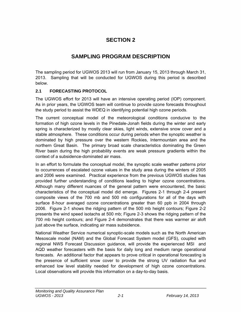
Monitoring and Quality Assurance Plan UGWOS - 2013 2-1 February 14, 2013
SECTION 2
SAMPLING PROGRAM DESCRIPTION
The sampling period for UGWOS 2013 will run from January 15, 2013 through March 31, 2013. Sampling that will be conducted for UGWOS during this period is described below.
2.1 FORECASTING PROTOCOL
The UGWOS effort for 2013 will have an intensive operating period (IOP) component. As in prior years, the UGWOS team will continue to provide ozone forecasts throughout the study period to assist the WDEQ in identifying potential high ozone periods.
The current conceptual model of the meteorological conditions conducive to the formation of high ozone levels in the Pinedale-Jonah fields during the winter and early spring is characterized by mostly clear skies, light winds, extensive snow cover and a stable atmosphere. These conditions occur during periods when the synoptic weather is dominated by high pressure over the western Rockies, Intermountain area and the northern Great Basin. The primary broad scale characteristics dominating the Green River basin during the high probability events are weak pressure gradients within the context of a subsidence-dominated air mass.
In an effort to formulate the conceptual model, the synoptic scale weather patterns prior to occurrences of escalated ozone values in the study area during the winters of 2005 and 2006 were examined. Practical experience from the previous UGWOS studies has provided further understanding of conditions leading to higher ozone concentrations. Although many different nuances of the general pattern were encountered, the basic characteristics of the conceptual model did emerge. Figures 2-1 through 2-4 present composite views of the 700 mb and 500 mb configurations for all of the days with surface 8-hour averaged ozone concentrations greater than 60 ppb in 2004 through 2006. Figure 2-1 shows the ridging pattern of the 500 mb height contours; Figure 2-2 presents the wind speed isotachs at 500 mb; Figure 2-3 shows the ridging pattern of the 700 mb height contours; and Figure 2-4 demonstrates that there was warmer air aloft just above the surface, indicating air mass subsidence.
National Weather Service numerical synoptic-scale models such as the North American Mesoscale model (NAM) and the Global Forecast System model (GFS), coupled with regional NWS Forecast Discussion guidance, will provide the experienced MSI and AQD weather forecasters with the basis for daily long and medium range operational forecasts. An additional factor that appears to prove critical in operational forecasting is the presence of sufficient snow cover to provide the strong UV radiation flux and enhanced low level stability needed for development of high ozone concentrations. Local observations will provide this information on a day-to-day basis.

Monitoring and Quality Assurance Plan UGWOS - 2013 2-2 February 14, 2013
Forecasts for Air Quality Division’s (AQDs) 2013 UGWOS ozone monitoring project will be issued by the MSI project meteorologists each morning. Once the forecast is completed it will be emailed to project participants by 10:00 MST each morning, seven days a week. The forecast will be finalized on a form containing three sections. The first section will be a synopsis of the current weather features that will affect the study area over at least the next 48 hours. The second section will contain a detailed short-term forecast out through day three. This forecast contains a discussion of temperature, wind, precipitation and sky conditions, and will also emphasize parameters that are of specific interest to the study, as appropriate, such as high pressure ridge location, inversion development, and snow cover. At the end of this section there will be a discussion on the expected ozone development during this period. The third section is an outlook that will cover days four through seven. This outlook will be similar in content to the second section with only the time frame changing.
Figure 2-1 Composite 500 mb Heights During High Ozone Periods
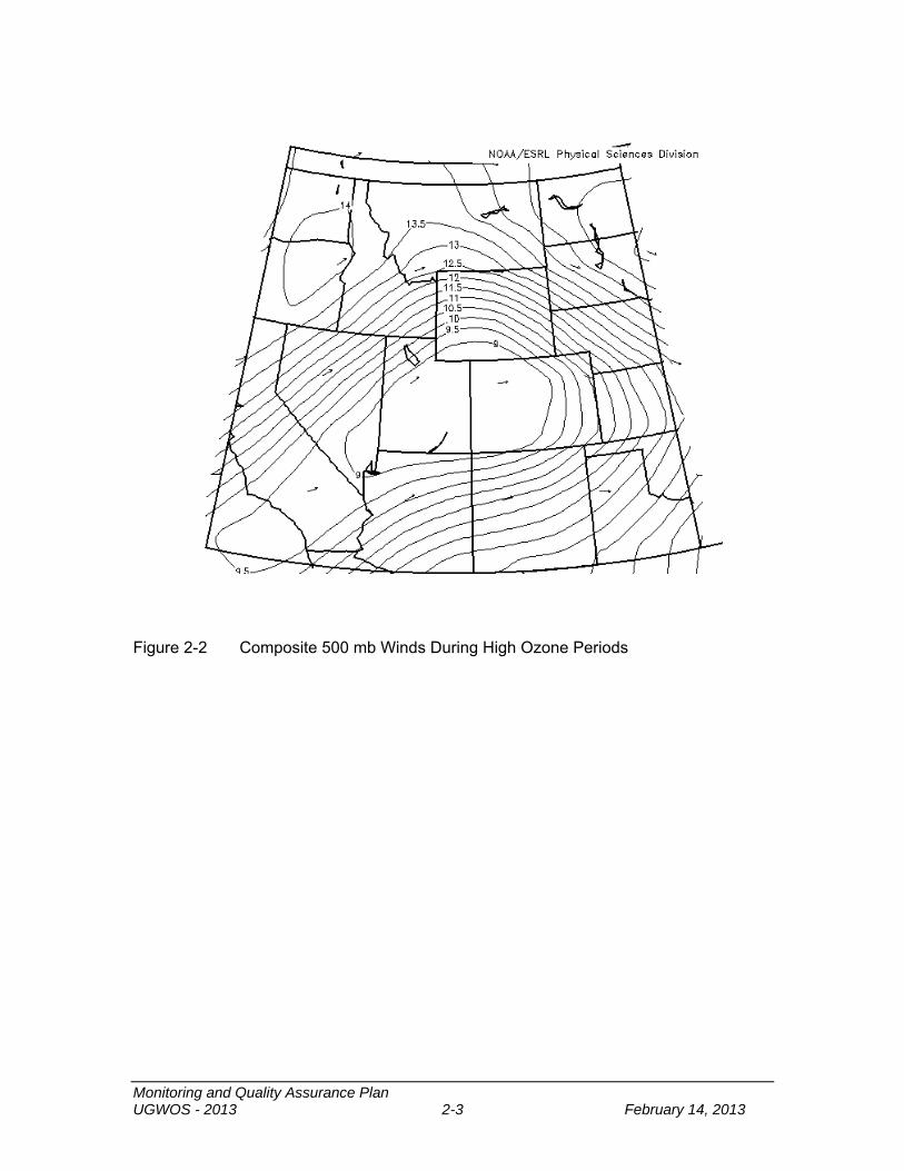
Monitoring and Quality Assurance Plan UGWOS - 2013 2-3 February 14, 2013
Figure 2-2 Composite 500 mb Winds During High Ozone Periods
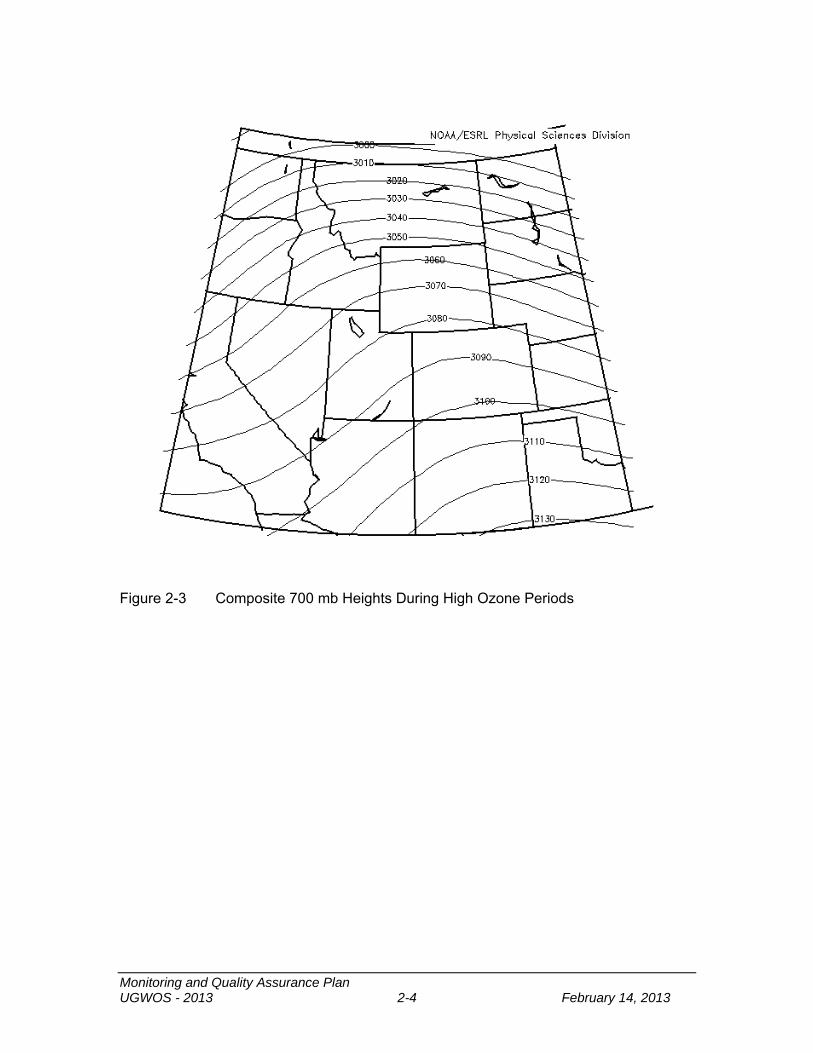
Monitoring and Quality Assurance Plan UGWOS - 2013 2-4 February 14, 2013
Figure 2-3 Composite 700 mb Heights During High Ozone Periods

Monitoring and Quality Assurance Plan UGWOS - 2013 2-5 February 14, 2013
Figure 2-4 Composite 700 mb Temperature During High Ozone Periods
2.2 CONTINUOUS MEASUREMENTS
Project-specific measurements to be continuously obtained over the complete field program period are presented below.

Monitoring and Quality Assurance Plan UGWOS - 2013 2-6 February 14, 2013
2.2.1 Mesonet Measurements
Surface ozone, wind, and temperature measurements will be taken from a 3-site mesonetwork (mesonet). In addition, each mesonet site will be equipped with a video camera, which will obtain images every 15 minutes. All sites will be equipped with cellular telemetry, allowing remote polling and real-time review of data.
The mesonet ozone analyzers will operate continuously over the course of the study and routine performance checks of the analyzers will be conducted approximately once per week. Their operation on-site will be checked using the 2-B ozone generator and zero-scrubber, and any zero and span deviations noted. As in previous UGWOS field programs, MSI will provide an on-site technician who will be stationed in the project area for the duration of the field season. The technician will provide field support and routine calibrations for the monitoring measurements for the Jonah site and the mesonet sites, and will deploy/retrieve VOC samples at the Jonah, Juel Springs, Big Piney, Boulder and mesonet sites (see below). He will also be available to troubleshoot issues at all AQD sites in the study area (Wyoming Range, Daniel, Boulder, Pinedale, Juel Springs, Big Piney and Farson meteorological tower). The field technician will also be available to assist with UGWOS and AQD contracted audits during the study period.
2.2.2 Ozone and NO/NOx Measurements in the Jonah Area
Continuous ozone and oxides of nitrogen will be performed at a location within the Jonah Field utilizing a WDEQ air monitoring trailer. Sampling at the Jonah site will include continuous measurement of ozone, oxides of nitrogen, wind speed, wind direction, temperature and pressure. The site will also be equipped with a video camera, providing 15-minute images. A datalogger and cellular telemetry will be supplied to retrieve data from the site on an hourly basis. Sites will be polled every 15 minutes to update data and post to project website. MSI will be responsible for the air quality and meteorological measurements, including routine checks, data validation, and database management.
2.2.3 SODAR Upper Level Winds
For the 2013 monitoring effort, the WDEQ MiniSodar (sodar) will be maintained at the existing WDEQ monitoring site at Boulder. Both surface and winds aloft will be measured continuously. The sodar is equipped with a battery bank, solar panels and a backup generator, providing continuous measurements without the need of AC power. However, the chosen site for operations does include available AC power. Remote communications is made possible with a cellular modem. All data will be posted in near real-time on a web page as well as archived data posted automatically on a FTP server. These sodar data can be reviewed remotely, as necessary.
The WDEQ will service the sodar, as necessary. T&B Systems will review the data on a daily basis, validate the wind data, and reduce mixing height data for the study period.

Monitoring and Quality Assurance Plan UGWOS - 2013 2-7 February 14, 2013
2.3 INTENSIVE MEASUREMENTS
During periods when high ozone levels are forecast, additional intensive measurements will be initiated. Up to 15 IOP days are budgeted for this study. IOP days will be identified using forecast information and consultation with WDEQ AQD. The key component of the IOPs is the collection of vertical profiles of ozone and meteorology profiles and VOC samples, as described below.
2.3.1 Ozone/rawinsonde Operations
Free ascending balloon-borne measurements of ozone, temperature, relative humidity, and winds will be made during each IOP from the Boulder air quality monitoring site by MSI personnel using equipment maintained by the WY DEQ. Twenty ozonesondes will be available for the study. It is anticipated that two ozonesondes will be released on a given IOP day.
MSI personnel will conduct the ozonesonde measurements. This includes preparation of the ozonesondes prior to the flights. MSI will dedicate one technician for conducting the ozonesonde measurements, with MSI’s dedicated UGWOS field technician available for backup support. Both technicians will be trained prior to the beginning of the study. At least one or two of the ozonesondes will be activated for the training.
2.3.2 VOC Sampling
VOC sampling will be conducted at the Boulder, Big Piney, and Juel Springs sites, as well as at the UGWOS-specific Jonah air quality site and the three mesonet sites. In addition to the sampling at the Jonah site, VOC samples will also be conducted at a second site located 450 meters NNE of the air quality site. This site is located away from the immediate influence of the gas production facility adjacent to the air quality site, and is also collecting wind data to assist in the comparison of readings from the two sites.
VOC will be sampled as integrated 3-hour samples. VOC samples will be collected using 6-liter SUMMA canisters connected to canister samplers previously used by the WDEQ for the Pinedale air toxics study conducted in 2009/2010 and with the existing canister sampling system at Boulder. Samples will be collected on IOP days from 0700-1000. Thus, up to 15 samples will be taken at each of the sites over the course of the study. In addition, five (5) quality control samples will be collected at each site, including zero air contamination samples, duplicates, and field blank samples.
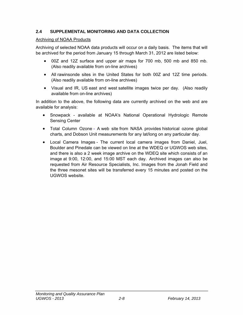
Monitoring and Quality Assurance Plan UGWOS - 2013 2-8 February 14, 2013
2.4 SUPPLEMENTAL MONITORING AND DATA COLLECTION
Archiving of NOAA Products
Archiving of selected NOAA data products will occur on a daily basis. The items that will be archived for the period from January 15 through March 31, 2012 are listed below:
00Z and 12Z surface and upper air maps for 700 mb, 500 mb and 850 mb. (Also readily available from on-line archives)
All rawinsonde sites in the United States for both 00Z and 12Z time periods. (Also readily available from on-line archives)
Visual and IR, US east and west satellite images twice per day. (Also readily available from on-line archives)
In addition to the above, the following data are currently archived on the web and are available for analysis:
Snowpack - available at NOAA's National Operational Hydrologic Remote Sensing Center
Total Column Ozone - A web site from NASA provides historical ozone global charts, and Dobson Unit measurements for any lat/long on any particular day.
Local Camera Images - The current local camera images from Daniel, Juel, Boulder and Pinedale can be viewed on line at the WDEQ or UGWOS web sites, and there is also a 2 week image archive on the WDEQ site which consists of an image at 9:00, 12:00, and 15:00 MST each day. Archived images can also be requested from Air Resource Specialists, Inc. Images from the Jonah Field and the three mesonet sites will be transferred every 15 minutes and posted on the UGWOS website.

Monitoring and Quality Assurance Plan UGWOS - 2013 3-1 February 14, 2013
SECTION 3
MONITORING SITE DESCRIPTIONS
Figure 3-1 presents a map of the UGWOS site locations. Table 3-1 presents coordinates for each of the sites. Photographs of the sites can be found in Appendix A.
Also included in Figure 3-1 and Table 3-1 are the locations of additional ozone monitoring sites, both past and present, in the study region.

Monitoring and Quality Assurance Plan UGWOS - 2013 3-2 February 14, 2013
Figure 3-1. Map of UGWOS and Additional Ozone Monitoring Site Locations

Monitoring and Quality Assurance Plan UGWOS - 2013 3-3 February 14, 2013
Table 3-1. Monitoring Locations
Latitude Longitude Elev.
SODAR SITE
Boulder 42.7188 -109.7529 7078’
MESONET SITES
Mesa 42.7774 -109.8829 7522’
Paradise 42.6825 -109.8090 6966’
Warbonnet 42.5703 -109.7022 7414’
JONAH AREA SITE
Jonah (2013) 42.4736 -109.6497 7259’
Jonah 2 VOC 42.4770 -109.6476 7300’
EXISTING MONITORING SITES OF INTEREST
Big Piney 42.4870 -110.0995 6823’
Daniel 42.7910 -110.0650 7084’
Castnet 42.9284 -109.7880 7853’
Farson 42.1184 -109.4541 6619’
Pinedale 42.8698 -109.8707 7186’
Juel Spring 42.3735 -109.5605 7020’
Wyoming Range 42.9801 -110.3530 8123’

Monitoring and Quality Assurance Plan UGWOS - 2013 4-1 February 14, 2013
SECTION 4
MONITORING EQUIPMENT DESCRIPTION
The following section describes the monitoring equipment that will be used for UGWOS. Measurement Quality Objectives (MQOs) are presented for each of the monitoring methods.
4.1 MESONET MONITORING SITES
All equipment used at the mesonet ozone monitoring sites will be housed in 70 to 100-quart insulated containers. Two 110 amp-hour deep cycle 12-Volt battery will power all equipment. Each site will be equipped with solar panels, allowing continuous monitoring and an Airlink Raven digital cellular modem for remote telecommunications.
The following equipment will be at each of the mesonet sites:
2B Model 202 Ozone Analyzer
The 2B Ozone Monitor will be used for the mesonet Monitoring. This monitor has a low power consumption (12v DC, 0.33 amp, 4.0 Watt) relative to conventional instruments allowing operation with deep cycle batteries. Additionally, it does not require a temperature-controlled environment. The 2B Technologies Model 202 Ozone Monitor™ is designed to enable accurate and precise measurements of ozone ranging from low ppb (precision of ~1 ppbv) up to 100,000 ppb (0-100 ppm) based on the well-established technique of absorption of light at 254 nm. "Absorption spectroscopy" is a chemical analysis technique made possible by the phenomenon that a given molecule absorbs light at selected wavelengths. The wavelengths absorbed are characteristic of each molecule’s atomic features. The amount of light radiation absorbed by a substance depends on two factors: the number of molecules in the path of the light, and the characteristics of the molecule (e.g., absorption cross-section). Measurement of changes in the light intensity as it passes through the molecules, and the use of calibration and reference data, enable the determination of the number of molecules encountered.
Accuracy (performance checks) 5%
Precision (performance checks) 5%
Resolution 0.001 ppm
Lower Quantifiable Limit 0.002 ppm
RM Young Model 05305 Wind Monitor AQ

Monitoring and Quality Assurance Plan UGWOS - 2013 4-2 February 14, 2013
For surface monitoring of wind speed and wind direction at the mesonet sites, we will employ RM Young 05305 Wind Monitor AQ wind speed and direction sensors. These sensors employ a propeller anemometer. The sensors will be mounted on 3-meter tripods (Figure 4-1), resulting in a measurement height of 3 meters. All sensors will be oriented to true north using either the GPS walk-off method or solar alignment method for orienting wind speed sensors.
Figure 4-1. Tripod mounting of wind sensors.
Monitoring quality objectives for the supplemental surface wind measurements are presented below.
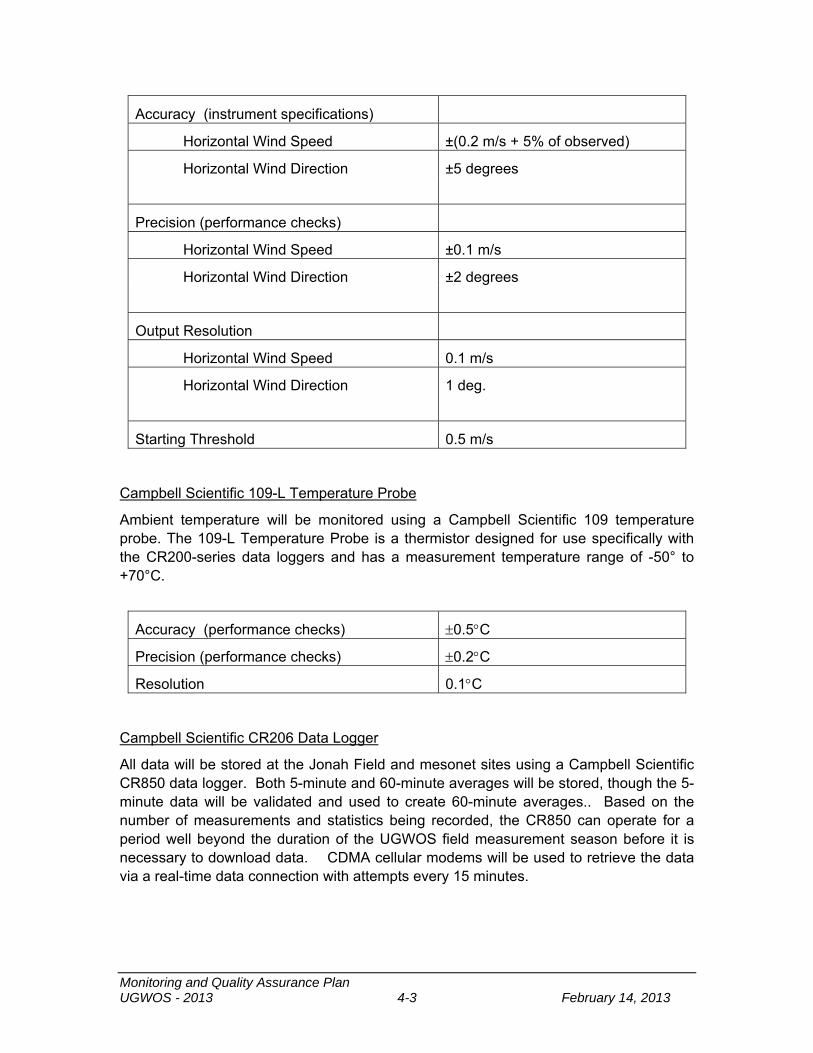
Monitoring and Quality Assurance Plan UGWOS - 2013 4-3 February 14, 2013
Accuracy (instrument specifications)
Horizontal Wind Speed ±(0.2 m/s + 5% of observed)
Horizontal Wind Direction ±5 degrees
Precision (performance checks)
Horizontal Wind Speed ±0.1 m/s
Horizontal Wind Direction ±2 degrees
Output Resolution
Horizontal Wind Speed 0.1 m/s
Horizontal Wind Direction 1 deg.
Starting Threshold 0.5 m/s
Campbell Scientific 109-L Temperature Probe
Ambient temperature will be monitored using a Campbell Scientific 109 temperature probe. The 109-L Temperature Probe is a thermistor designed for use specifically with the CR200-series data loggers and has a measurement temperature range of -50° to +70°C.
Accuracy (performance checks) 0.5C
Precision (performance checks) 0.2C
Resolution 0.1C
Campbell Scientific CR206 Data Logger
All data will be stored at the Jonah Field and mesonet sites using a Campbell Scientific CR850 data logger. Both 5-minute and 60-minute averages will be stored, though the 5-minute data will be validated and used to create 60-minute averages.. Based on the number of measurements and statistics being recorded, the CR850 can operate for a period well beyond the duration of the UGWOS field measurement season before it is necessary to download data. CDMA cellular modems will be used to retrieve the data via a real-time data connection with attempts every 15 minutes.
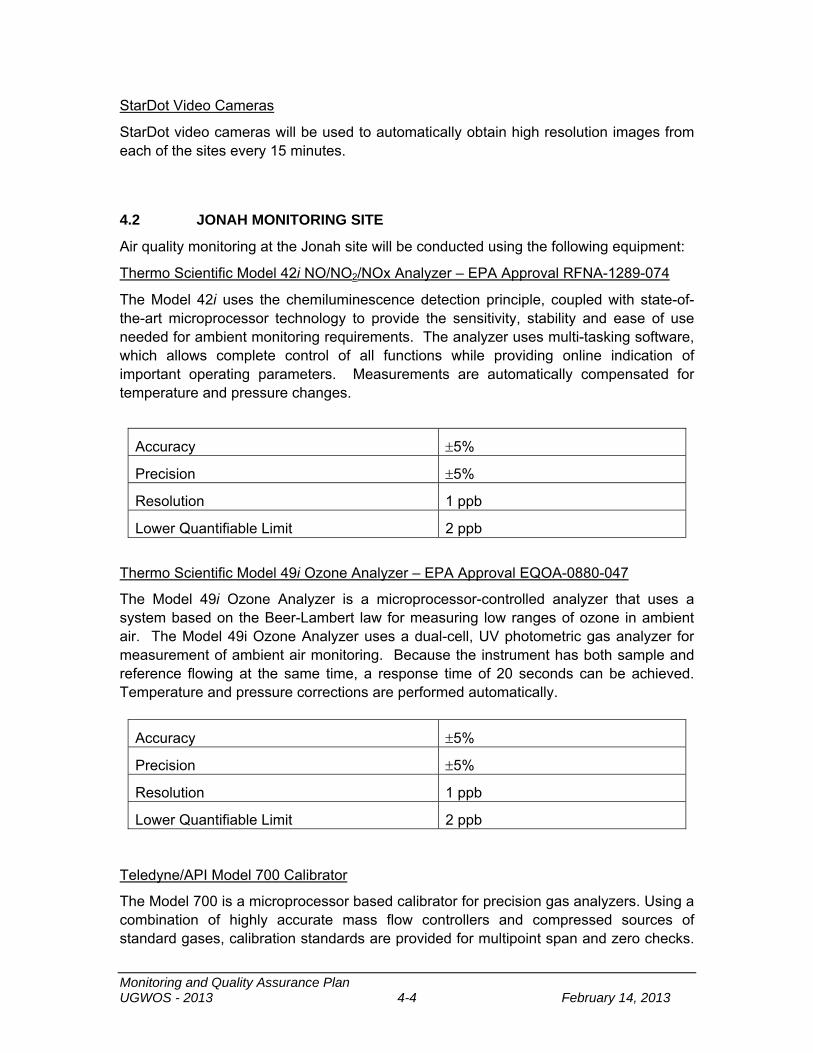
Monitoring and Quality Assurance Plan UGWOS - 2013 4-4 February 14, 2013
StarDot Video Cameras
StarDot video cameras will be used to automatically obtain high resolution images from each of the sites every 15 minutes.
4.2 JONAH MONITORING SITE
Air quality monitoring at the Jonah site will be conducted using the following equipment:
Thermo Scientific Model 42i NO/NO2/NOx Analyzer – EPA Approval RFNA-1289-074
The Model 42i uses the chemiluminescence detection principle, coupled with state-of-the-art microprocessor technology to provide the sensitivity, stability and ease of use needed for ambient monitoring requirements. The analyzer uses multi-tasking software, which allows complete control of all functions while providing online indication of important operating parameters. Measurements are automatically compensated for temperature and pressure changes.
Accuracy 5%
Precision 5%
Resolution 1 ppb
Lower Quantifiable Limit 2 ppb
Thermo Scientific Model 49i Ozone Analyzer – EPA Approval EQOA-0880-047
The Model 49i Ozone Analyzer is a microprocessor-controlled analyzer that uses a system based on the Beer-Lambert law for measuring low ranges of ozone in ambient air. The Model 49i Ozone Analyzer uses a dual-cell, UV photometric gas analyzer for measurement of ambient air monitoring. Because the instrument has both sample and reference flowing at the same time, a response time of 20 seconds can be achieved. Temperature and pressure corrections are performed automatically.
Accuracy 5%
Precision 5%
Resolution 1 ppb
Lower Quantifiable Limit 2 ppb Teledyne/API Model 700 Calibrator
The Model 700 is a microprocessor based calibrator for precision gas analyzers. Using a combination of highly accurate mass flow controllers and compressed sources of standard gases, calibration standards are provided for multipoint span and zero checks.

Monitoring and Quality Assurance Plan UGWOS - 2013 4-5 February 14, 2013
Up to 4 gas sources may be used. In addition, the Model 700 is equipped with an optional built-in, programmable ozone generator for accurate, dependable ozone calibrations and to produce NO2 when blended with NO gas in the internal GPT chamber. As many as 50 independent calibration sequences may be programmed into the M700, covering time periods of up to one year. These sequences may be actuated manually, automatically, or by a remote signal. Dilution air is supplied to the calibrator using an API Model 701 zero air system.
RM Young Model 05305 Wind Monitor AQ
For monitoring of wind speed and wind direction a 10-meter tower and RM Young 05305 Wind Monitor AQ wind speed and direction sensor will be employed. These sensors use a propeller-type anemometer. The direction vane will be oriented to true north using either a compass or the GPS walkoff method.
Accuracy (instrument specifications)
Horizontal Wind Speed ±(0.2 m/s + 5% of observed)
Horizontal Wind Direction ±5 degrees
Precision
Horizontal Wind Speed ±0.1 m/s
Horizontal Wind Direction ±2 degrees
Output Resolution
Horizontal Wind Speed 0.1 m/s
Horizontal Wind Direction 1 deg.
Starting Threshold 0.5 m/s
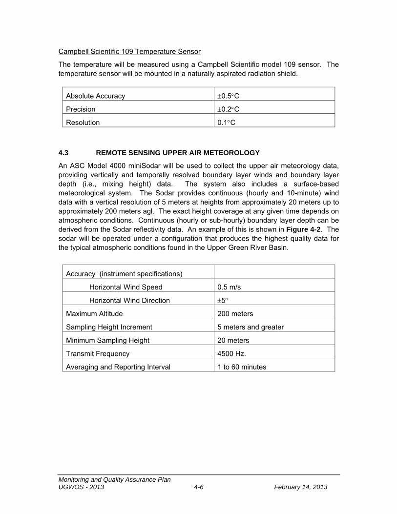
Monitoring and Quality Assurance Plan UGWOS - 2013 4-6 February 14, 2013
Campbell Scientific 109 Temperature Sensor
The temperature will be measured using a Campbell Scientific model 109 sensor. The temperature sensor will be mounted in a naturally aspirated radiation shield.
Absolute Accuracy 0.5C
Precision 0.2C
Resolution 0.1C
4.3 REMOTE SENSING UPPER AIR METEOROLOGY
An ASC Model 4000 miniSodar will be used to collect the upper air meteorology data, providing vertically and temporally resolved boundary layer winds and boundary layer depth (i.e., mixing height) data. The system also includes a surface-based meteorological system. The Sodar provides continuous (hourly and 10-minute) wind data with a vertical resolution of 5 meters at heights from approximately 20 meters up to approximately 200 meters agl. The exact height coverage at any given time depends on atmospheric conditions. Continuous (hourly or sub-hourly) boundary layer depth can be derived from the Sodar reflectivity data. An example of this is shown in Figure 4-2. The sodar will be operated under a configuration that produces the highest quality data for the typical atmospheric conditions found in the Upper Green River Basin.
Accuracy (instrument specifications)
Horizontal Wind Speed 0.5 m/s
Horizontal Wind Direction 5
Maximum Altitude 200 meters
Sampling Height Increment 5 meters and greater
Minimum Sampling Height 20 meters
Transmit Frequency 4500 Hz.
Averaging and Reporting Interval 1 to 60 minutes

Monitoring and Quality Assurance Plan UGWOS - 2013 4-7 February 14, 2013
Figure 4-2. Example of sodar backscatter data capturing the daytime mixing height layers under cold wintertime conditions.
4.4 OZONE/RAWINSONDES
To profile ozone concentrations from the surface to the tropopause, we will use balloon-borne ozonesondes, with measurements placed at the Boulder air quality site. The ozonesonde system has three primary components, described below:
iMet-3050 403 MHz GPS Upper-Air Sounding System
The iMet-3050 is an automated sounding system that operates in the 403 MHz meteorological frequency band. Pressure, temperature, and humidity data (PTU) are collected by the radiosonde and transmitted to the ground station by a digitally coded message sent once per second.
The System Computer receives the PTU data, the radiosonde GPS data, and the differential GPS data that is then processed by the iMetOS into meteorological data and met products. iMetOS also provides graphical displays, data communications and archiving capabilities.
iMet-1 RSB Radiosondes
The iMet-1 RSB radiosonde is 9 x 9 x 18 cm, weighs 260 grams, and is powered by an alkaline dry cell battery. The radiosonde transmitter sends its modulated signals in the 403 MHz range. Temperature is measured using a bead thermistor and relative humidity using a capacitive hygristor. The iMet-1 RSB incorporates a low-noise integrated circuit GPS receiver. Winds aloft are calculated from the change in balloon position (determined from navaid) with time. Height is obtained directly from GPS positioning and, unlike older systems, pressure is now a derived parameter, calculated from the hydrostatic equation, using measured height, temperature, and humidity.
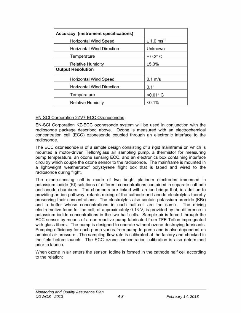
Monitoring and Quality Assurance Plan UGWOS - 2013 4-8 February 14, 2013
Accuracy (instrument specifications)
Horizontal Wind Speed ± 1.0 ms-1
Horizontal Wind Direction Unknown
Temperature ± 0.2 C
Relative Humidity ±5.0% Output Resolution
Horizontal Wind Speed 0.1 m/s
Horizontal Wind Direction 0.1
Temperature <0.01 C
Relative Humidity <0.1%
EN-SCI Corporation 2ZV7-ECC Ozonesondes
EN-SCI Corporation KZ-ECC ozonesonde system will be used in conjunction with the radiosonde package described above. Ozone is measured with an electrochemical concentration cell (ECC) ozonesonde coupled through an electronic interface to the radiosonde.
The ECC ozonesonde is of a simple design consisting of a rigid mainframe on which is mounted a motor-driven Teflon/glass air sampling pump, a thermistor for measuring pump temperature, an ozone sensing ECC, and an electronics box containing interface circuitry which couple the ozone sensor to the radiosonde. The mainframe is mounted in a lightweight weatherproof polystyrene flight box that is taped and wired to the radiosonde during flight.
The ozone-sensing cell is made of two bright platinum electrodes immersed in potassium iodide (KI) solutions of different concentrations contained in separate cathode and anode chambers. The chambers are linked with an ion bridge that, in addition to providing an ion pathway, retards mixing of the cathode and anode electrolytes thereby preserving their concentrations. The electrolytes also contain potassium bromide (KBr) and a buffer whose concentrations in each half-cell are the same. The driving electromotive force for the cell, of approximately 0.13 V, is provided by the difference in potassium iodide concentrations in the two half cells. Sample air is forced through the ECC sensor by means of a non-reactive pump fabricated from TFE Teflon impregnated with glass fibers. The pump is designed to operate without ozone-destroying lubricants. Pumping efficiency for each pump varies from pump to pump and is also dependent on ambient air pressure. The sampling flow rate is calibrated at the factory and checked in the field before launch. The ECC ozone concentration calibration is also determined prior to launch.
When ozone in air enters the sensor, iodine is formed in the cathode half cell according to the relation:
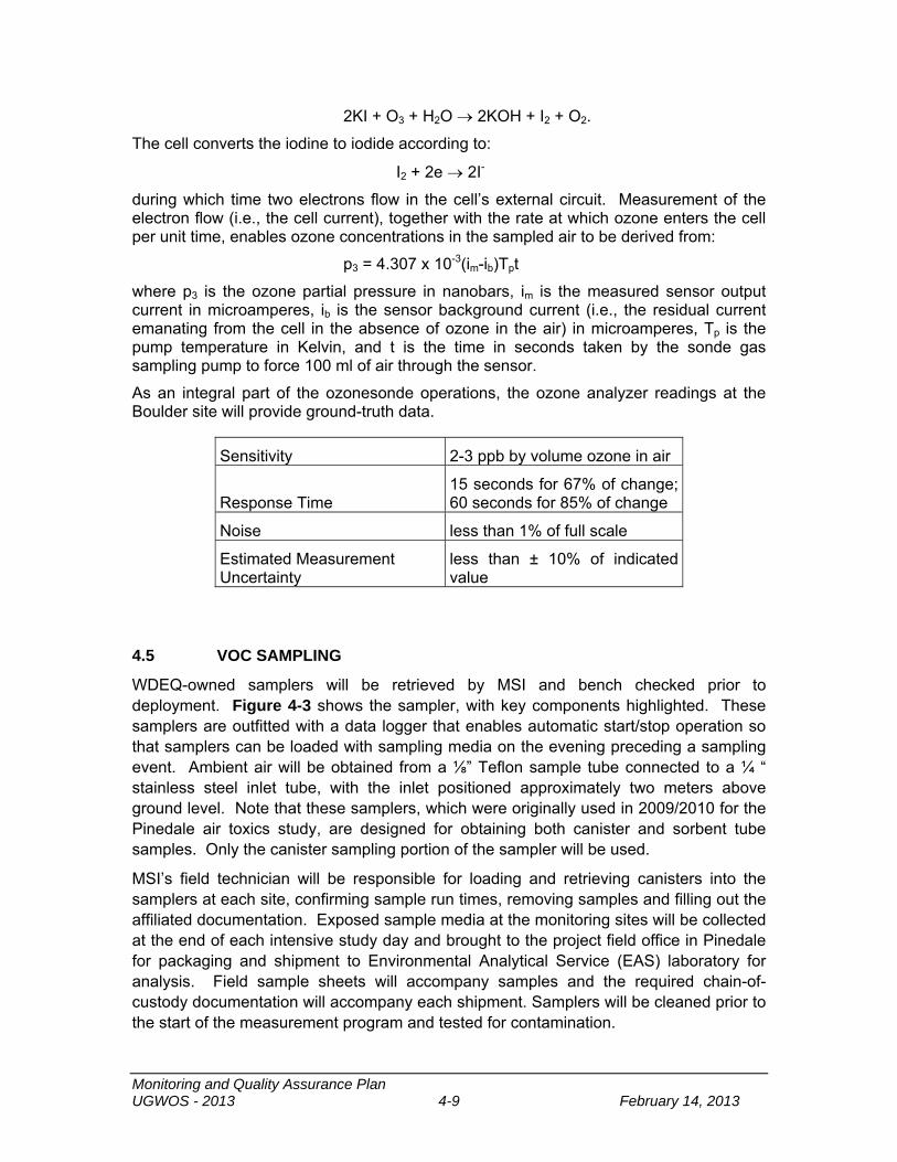
Monitoring and Quality Assurance Plan UGWOS - 2013 4-9 February 14, 2013
2KI + O3 + H2O 2KOH + I2 + O2.
The cell converts the iodine to iodide according to:
I2 + 2e 2I-
during which time two electrons flow in the cell’s external circuit. Measurement of the electron flow (i.e., the cell current), together with the rate at which ozone enters the cell per unit time, enables ozone concentrations in the sampled air to be derived from:
p3 = 4.307 x 10⁻³(im-ib)Tpt
where p3 is the ozone partial pressure in nanobars, im is the measured sensor output current in microamperes, ib is the sensor background current (i.e., the residual current emanating from the cell in the absence of ozone in the air) in microamperes, Tp is the pump temperature in Kelvin, and t is the time in seconds taken by the sonde gas sampling pump to force 100 ml of air through the sensor.
As an integral part of the ozonesonde operations, the ozone analyzer readings at the Boulder site will provide ground-truth data.
4.5 VOC SAMPLING
WDEQ-owned samplers will be retrieved by MSI and bench checked prior to deployment. Figure 4-3 shows the sampler, with key components highlighted. These samplers are outfitted with a data logger that enables automatic start/stop operation so that samplers can be loaded with sampling media on the evening preceding a sampling event. Ambient air will be obtained from a ⅛” Teflon sample tube connected to a ¼ “ stainless steel inlet tube, with the inlet positioned approximately two meters above ground level. Note that these samplers, which were originally used in 2009/2010 for the Pinedale air toxics study, are designed for obtaining both canister and sorbent tube samples. Only the canister sampling portion of the sampler will be used.
MSI’s field technician will be responsible for loading and retrieving canisters into the samplers at each site, confirming sample run times, removing samples and filling out the affiliated documentation. Exposed sample media at the monitoring sites will be collected at the end of each intensive study day and brought to the project field office in Pinedale for packaging and shipment to Environmental Analytical Service (EAS) laboratory for analysis. Field sample sheets will accompany samples and the required chain-of- custody documentation will accompany each shipment. Samplers will be cleaned prior to the start of the measurement program and tested for contamination.
Sensitivity 2-3 ppb by volume ozone in air
Response Time 15 seconds for 67% of change; 60 seconds for 85% of change
Noise less than 1% of full scale
Estimated Measurement Uncertainty
less than ± 10% of indicated value
Monitoring and Quality Assurance Plan UGWOS - 2013 4-10 February 14, 2013
VOC samples will be analyzed using Method TO-14 with an expanded PAMS list of compounds (see Table 4-1). Analysis will be performed by Environmental Analytical Services, Inc., San Luis Obispo, CA.
Figure 4-3. Canister Sampler. Only those components associated with the SUMMA canister will be employed.
Monitoring and Quality Assurance Plan UGWOS - 2013 4-11 February 14, 2013
Table 4-1. Target compound list for EPA Method TO-14 Toxics in Air (Expanded for PAMS).
Ethene Cyclohexane Total Petroleum Hydrocarbons: Acetylene 2-Methylhexane Total Non-Methane Hydrocarbons Ethane 2,3-Dimethylpentane Propene 3-Methylhexane Propane 2-Methyl-1hexene i-Butane Tert amyl methyl ether Methanol 2,2,4-Trimethylpentane 1-Butene n-Heptane 1,3-Butadiene Methylcyclohexane n-Butane 2,5-Dimethylhexane t-2-Butene 2,4-Dimethylhexane c-2-Butene 2,3,4-Trimethylpentane Ethanol Toluene Sample: Composition3-Methyl-1-butene 2,3-Dimethylhexane Total IdentifiedAcetone 2-Methylheptane Paraffinsi-Pentane 4-Methylheptane Isoparaffins1-Pentene 3-Ethyl-3-methylpentane AromaticsIsopropanol 3-Methylheptane Napthlenes2-Methyl-1-butene 2-Methyl-1-heptene Olefinsn-Pentane n-Octane OxygenatesIsoprene Ethylbenzene t-2-Pentene m,p-xylene c-2-Pentene Styrene Tert butyl alcohol o-xylene 2-Methyl-2-butene 1-Nonene 2,2-Dimethylbutane n-Nonane Cyclopentene i-Propylbenzene n-Propanol n-propylbenzene Cyclopentane a-Pinene Methyl tert butyl ether 3-Ethyltoluene 2,3-Dimethylbutane 4-Ethyltoluene 2-Methylpentane 1,3,5-Trimethylbenzene3-Methylpentane 2-Ethyltoluene1-Hexene b-Pinenen-Hexane 1,2,4-TrimethylbenzeneDiisopropyl ether n-Decane3-Methylcyclopentene 1,2,3-TrimethylbenzeneEthyl tert butyl ether IndanMethylcyclopentane d-Limonene 2,4-Dimethylpentane 1,3-DiethylbenzeneBenzene
Dodecane
1,4-Diethylbenzenen-Butylbenzene1,4-Dimethyl-2-ethylbenzene1,3-Dimethyl-4-ethylbenzene1,2-Dimethyl-4-ethylbenzeneUndecane1,2,4,5-Tetramethylbenzene1,2,3,5-TetramethylbenzeneNapthalene
Monitoring and Quality Assurance Plan UGWOS - 2013 5-1 February 14, 2013
SECTION 5
DATA REPORTING
5.1 DATA MANAGEMENT PLAN
A primary study objective is to produce an adequately validated data set from the field measurements that is well defined and documented, and available to researchers in a timely manner. The overall goal of the data management effort is to create a system that is straightforward and easy for users to obtain data and provide updates.
MSI will collect all measurements remotely on at least an hourly basis. Preliminary data will be posted on a near real-time basis on a password-protected UGWOS web site at http://ugwos.metsolution.com. Both 5-minute and hourly averages will be stored in data acquisition systems 5-minute data will be validated and used to calculate hourly averages. The data loggers are all equipped with internal memory that can store data for the duration of the study. Thus, if telemetry fails at a given site, data can be collected manually. All polled data are backed up at least daily, minimizing the chance of data loss. Camera images as well as daily forecasts will be displayed on the web site. Figures 5-1 and 5-2 are example graphics that will be presented on the internal website.
Each data provider will be responsible for reviewing and validating their collected data. The raw data will be validated to Level 1 as described in “The Measurement Process: Precision, Accuracy, and Validity” (Watson, 2001) before being submitted to the database. This includes flagging values for instrument downtime and performance tests, applying any adjustments for calibration deviation, investigating extreme values and applying appropriate quality control codes. Quality control codes used for UGWOS include simple validation codes as well as AQS null codes developed by the EPA and are presented in Table 5-1. Each data provider will be responsible for documenting the validation process so that it could be provided to the data manager and other analysts, if needed.
In addition, each data provider will be responsible for furnishing information regarding the monitoring equipment used in the field study and any additional site information to the data manager, as requested, to enhance the overall documentation of the study. In particular, participants will provide the Monitoring Quality Objective (MQOs) defining the quality of all data submitted as “valid.” These MQOs contain the following:
Accuracy Precision Lower quantifiable limit Resolution Completeness
If cases exist where data do not meet the primary MQOs but are still deemed useable and can be defined with a secondary set of MQOs, these additional MQOs and the dates to which they apply will also be submitted.
Monitoring and Quality Assurance Plan UGWOS - 2013 5-2 February 14, 2013
Figure 5-1 – Ambient Ozone Concentration Map
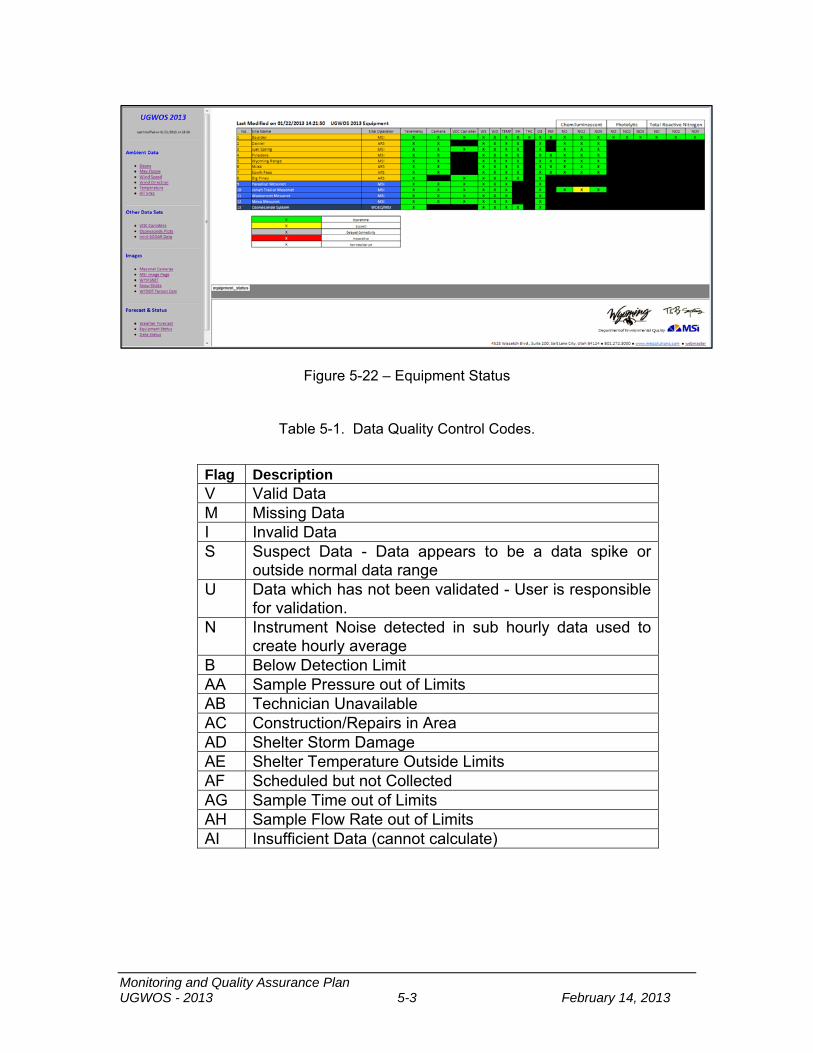
Monitoring and Quality Assurance Plan UGWOS - 2013 5-3 February 14, 2013
Figure 5-22 – Equipment Status
Table 5-1. Data Quality Control Codes.
Flag Description V Valid Data M Missing Data I Invalid Data S Suspect Data - Data appears to be a data spike or
outside normal data range U Data which has not been validated - User is responsible
for validation. N Instrument Noise detected in sub hourly data used to
create hourly average B Below Detection Limit AA Sample Pressure out of Limits AB Technician Unavailable AC Construction/Repairs in Area AD Shelter Storm Damage AE Shelter Temperature Outside Limits AF Scheduled but not Collected AG Sample Time out of Limits AH Sample Flow Rate out of Limits AI Insufficient Data (cannot calculate)
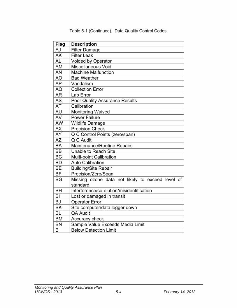
Monitoring and Quality Assurance Plan UGWOS - 2013 5-4 February 14, 2013
Table 5-1 (Continued). Data Quality Control Codes.
Flag Description AJ Filter Damage AK Filter Leak AL Voided by Operator AM Miscellaneous Void AN Machine Malfunction AO Bad Weather AP Vandalism AQ Collection Error AR Lab Error AS Poor Quality Assurance Results AT Calibration AU Monitoring Waived AV Power Failure AW Wildlife Damage AX Precision Check AY Q C Control Points (zero/span) AZ Q C Audit BA Maintenance/Routine Repairs BB Unable to Reach Site BC Multi-point Calibration BD Auto Calibration BE Building/Site Repair BF Precision/Zero/Span BG Missing ozone data not likely to exceed level of
standard BH Interference/co-elution/misidentification BI Lost or damaged in transit BJ Operator Error BK Site computer/data logger down BL QA Audit BM Accuracy check BN Sample Value Exceeds Media Limit B Below Detection Limit
Monitoring and Quality Assurance Plan UGWOS - 2013 5-5 February 14, 2013
Once the data have been validated to Level 1, the data will be prepared for submittal to the database in a form that clearly defines the time reference, averaging period, parameter names and units. The time reference for the database is local standard time (Mountain Standard Time) and the averaging period reference will be standardized to hour beginning (0 – 23). The data will be submitted as ASCII comma delimited text files or excel spreadsheet files, with data columns well defined to clarify site identification, parameters, instrumentation, units, and time reference.
Data will be submitted in a format similar to that of the final database structure, as outlined below. This basically has a second column for each measured value for an accompanying QC code. QC codes include simple validation codes as well as AQS null codes developed by the EPA.
Database Management Design
MSI will be responsible for assimilating the submitted data into an integrated relational Microsoft ACCESS database and is managing the data for subsequent distribution and analysis. The database will consist of both information and data files. The goal is to make the database very usable by data analysts and all participants.
The following describes the design for the database, which was similarly implemented during the 2007, 2008, 2009 and 2010 field studies. The database includes an inventory spreadsheet file to help users track and ensure that all of the data were submitted and processed in a timely and consistent manner. All data files submitted will be examined to verify unique names for all sites, instruments, and parameters so that no orphan or duplicate records exist in any of the tables. A system is in place for identifying the version and or modification date of all data files. All files are backed up daily.
The data have the following flat format:
Surface Hourly Meteorological Data
SITE, DATE, HOUR, WS, WS_QC, WD, WD_QC, TP, TP_QC, and any additional met parameters and QC codes, if collected.
Ozone 8-hour averaged:
SITE, DATE, HOUR, O3_8HR, O38HR_QC
Hourly Surface Air Quality:
SITE, DATE, HOUR, OZONE, O3_QC, NO, NO_QC, NOx, NOx_QC, NOy, NOy_QC, PAN, PAN_QC and any additional air quality parameters if collected and QC codes.
Upper level meteorological and air quality data
SODAR data will be stored in both a flat file format and a CDF (common data format) or similar tabular format. CDF files are used for plotting the data. Participants should include both flat files and CDF files with their data submissions. The final flat format will be as follows:

Monitoring and Quality Assurance Plan UGWOS - 2013 5-6 February 14, 2013
SITE, DATE, HOUR, TIME, HEIGHT, WS, WS_QC, WD, WD_QC
Radiosonde and Ozonesonde data will also be collected during IOPs. These data are assembled in Sonde Data (met) and Sonde Data (ozone) data tables. GPS coordinates and elevation (by altimeter and GPS reading) as well as meteorological and ozone readings will be available in these tables.
VOC Canister Data
VOC canisters will be collected during IOPs. The canister data is analyzed using the TO-14 method by EAS. Data files are formatted in a similar format to what is uploaded into the database. VOC data will be presented in two data tables. VOC will have individual compounds presented by canister sample and sample date. A second table in the database will have a summary of compound classifications.
The data will be formatted into the final database with the following unit configurations and naming conventions:
Parts per billion (ppb) for O3, NO, NO2, and NOx Meters per second for wind speed (as a general rule, metric units will be used) Degrees Celsius for ambient temperature Watts/m2 for radiation
Micrograms per cubic meter, parts per billion by volume, and parts per billion by Carbon for VOC canister data
SITE = Alpha-numeric site code identifier DATE = (MM/DD/YY) HOUR= Nearest whole begin hour (HH) (MST) TIME, START_TIME or END_TIME = Time stamp of data (HH:MM:SS) (MST) HEIGHT = Elevation in meters above MSL QC_CODE, WS_QC, WD_QC, O3_QC, etc =
“V” (valid), “M” (missing), “I” (invalid), “S” (secondary MQOs) NOTES = any additional information
The Level 1 data files along with the documentation files will be available for download on an FTP server.
5.2 DATA REPORTING
Files of all data collected during the study will be transmitted to WDEQ by June 1, 2013.
The team will review the validated data collected during the field study and prepare descriptive summaries in a report format for delivery to WDEQ. The Team will prepare summaries of air quality and meteorological conditions during the study period. In addition, the Team will prepare more detailed descriptive analyses of the air quality and meteorology measured during any high ozone events during the study period. As part of the Level 1 data validation procedures, the Team will carefully examine all of the measurements. This process typically provides insight into the critical processes that determine the extent of pollution loading such as atmospheric stability, wind shear (low-

Monitoring and Quality Assurance Plan UGWOS - 2013 5-7 February 14, 2013
level jets, etc), layers aloft, and boundary layer development (growth rate, peak mixing heights), including the nocturnal boundary, convective boundary, and residual layer. The meteorology leading up to and during periods with high ozone levels and the diurnal behavior of ozone aloft during these periods will be characterized.
Supporting the analyses discussion, products that will be produced in this phase of the study include but are not limited to:
1. Time-series plots of continuous measurements such as ozone, ambient temperature, radiation;
2. Vertical profiles of winds;
3. Wind roses at the surface;
4. Pollution roses at the surface; and
5. Summary tables of 1-hour and 8-hour averaged ozone as well as statistical summaries showing hourly averages and maximums.
A final report will be prepared presenting:
The above-mentioned information and associated analyses in an easy to comprehend format.
A summary of field operations. A measure of the associated data capture rates will be included. Problems encountered during the field operations will be discussed.
Details of the database design including descriptions of the metafiles; field descriptors; and the accuracy, precision, lower limits, resolution, and completeness of each measurement.
A draft version of the report will be provided to WDEQ by July 1, 2013. Voluminous tables and figures will be incorporated into electronic appendices as appropriate. All report materials will be made available via a secure FTP transfer site.

Monitoring and Quality Assurance Plan UGWOS - 2013 6-1 February 14, 2013
SECTION 6
QUALITY ASSURANCE PROGRAM
6.1 PROJECT MANAGEMENT
Mr. George Wilkerson will serve as overall project manager. Mr. Bill Hauze will serve as the Field Operations Manager for the study. He will be responsible for coordinating and verifying corrective action for any measurement-related problems.
An organizational chart for UGWOS 2013 is provided in Figure 6-1. Study personnel responsibilities and contact information are presented in Table 6-1.
While it is not anticipated that the scope of the monitoring effort will change over the relatively short duration of the effort, any changes will result in a revised version of this QAPP. Mr. David Bush is responsible for the writing and distribution of the QAPP. Revisions will be distributed based on the distribution list at the beginning of this document.
6.2 DATA QUALITY OBJECTIVES
Specific measurement quality objectives have been presented for each measurement in Section 4 of this document. The overall objectives for the collection of valid data will be as follows:
Air quality data: 80% of the possible data
Meteorological data: 90% of the possible data
For the above calculation, data lost during calibrations, maintenance or audits are considered invalid.
6.3 ASSESSMENT AND OVERSIGHT
QUALITY CONTROL PROCEDURES
As part of the quality assurance program, detailed quality control procedures have been implemented to assess and maintain control of the quality of the data collected. All equipment will undergo complete checkout and acceptance prior to the start of monitoring on January 15, 2013. This checkout will occur during the weeks prior to the start of monitoring, as well as during setup and installation of the equipment. Standard operating procedures (SOPs) for measurements will be developed for key monitoring activities. SOPs can be found in Appendix B.

Monitoring and Quality Assurance Plan UGWOS - 2013 6-2 February 14, 2013
Figure 6-1. Project organization.

Monitoring and Quality Assurance Plan UGWOS - 2013 6-3 February 14, 2013
Table 6-2. Project responsibilities and contacts
Name Organization Key Responsibilities Phone Numbers
Cara Keslar Wyoming DEQ Contract Manager (307) 777-8684
(307) 286-2383 (cell)
Jennifer Frazier Wyoming DEQ General study support (307) 7497912 (cell)
Ryan McCammon Wyoming DEQ Forecasting (307) 777-7104
George Wilkerson MSI Project Manager (801) 272-3000 Ext. 304
Bill Hauze MSI Field Manager, Reporting (801) 272-3000 Ext. 308
(801) 450-3776 (cell)
Dan Risch MSI Forecasting (801) 272-3000 Ext. 306
Casey Lenhart MSI Measurement System and Remote Telemetry Configuration and Testing
(801) 272-3000 Ext. 307
Brian Olsen MSI Data polling
Data processing and validation, Reporting
(801) 272-3000 Ext. 311
Scott Adamson MSI Database and Data Validation, Reporting
(801)-272-3000 Ext. 302
Tyler Ward MSI Full-time onsite field technician
(928) 814-3926 (cell)
David Bush T&B Systems Quality Assurance
QAPP
(530) 647-1169
(530) 903-6831 (cell)
Bob Baxter T&B Systems Sodar operations (661) 294-1103
(661) 645-0526 (cell)
David Yoho T&B Systems Quality Assurance audits
(661) 294-1103
(661) 212-3008 (cell)
A summary of key elements of the QC program for each measurement is presented below:
Station Checks
Performance of all UGWOS 2013 Jonah monitoring site equipment will be checked daily via remote polling, with site visits occurring at least weekly.
Ozone Transfer Standards
All ozone analyzers and samplers will be routinely checked using a certified transfer standard, following operating procedures consistent with EPA guidelines. For FEM ozone analyzer, these checks will be conducted using a transfer standard certified against a primary standard maintained following EPA’s guidelines at MSI’s office in Salt Lake City, UT. For the mesonet equipment, a 2B model 306 (S/N 2) portable ozone calibrator will be used. This portable ozone calibrator will also be compared regularly against MSI’s primary standard. A pass/fail criterion of +/-10% will be used when
Monitoring and Quality Assurance Plan UGWOS - 2013 6-4 February 14, 2013
evaluating the span and calibration data, after which corrective measures will be implemented.
Mesonet Analyzers
Mesonet 2B ozone analyzers will be checked using certified standards, following operating procedures consistent with EPA guidelines. This will consist of zero, precision, and span checks conducted at least weekly.
Jonah Ozone, NO/NOx Analyzers
Analyzers for the UGWOS 2013 Jonah monitoring effort will be checked using certified standards, following operating procedures consistent with EPA guidelines. This will consist of zero, precision, and span checks conducted automatically every 3 days.
VOC Canister Sampling Systems
Tripod mounted portable VOC canister sampling systems will be flushed with ultrapure air and checked for contamination prior to the start of the UGWOS 2013 study. VOC canisters will be installed in each system, allowed to sample ultrapure air through the system inlet, and sent to the analytical laboratory for analysis to confirm that systems are free of contamination.
The siting of the Jonah VOC measurements will be verified throughout the study by installing an additional VOC sampler (Jonah 2) several hundred meters away from potential sources near the Jonah site. Samples from both locations will be collected and compared to evaluate whether or not measurements from the Jonah location are biased by local sources.
MiniSodar
The status of the instruments will be checked daily via remote access of the data. If any problems are encountered that could affect data recovery, repairs will be made promptly. The data will be transferred hourly to T&B’s server, using a cellular modem. Data can also be accessed in real time via a web site so that team members can use the data to assist in special monitoring and forecasting. The link to the web site is: http://tbsys.serveftp.net/ugwossodar/.
CALIBRATIONS
The purpose of a calibration is to establish a relationship between the ambient conditions and an instrument's response by challenging the instrument with known values and adjusting the instrument to respond properly to those values. The calibration method for each of the air quality and meteorological variables is summarized in Table 6-3.
Calibrations of the ozone instruments and the NO/NOx analyzer will be performed upon initial installation and at the end of the study period. Additional calibrations will be performed on an as-needed basis in the event of equipment repair or replacement. All calibrations will be performed in accordance with manufacturers’ recommendations and consistent with USEPA guidance (USEPA, 1994, 1995, 2000).

Monitoring and Quality Assurance Plan UGWOS - 2013 6-5 February 14, 2013
Calibrations and zero/span checks of all ozone monitoring equipment will be conducted using a transfer standard certified against MSI’s primary standard, which is maintained following EPA’s guidelines at their office in Salt Lake City, UT, as well as against the US EPA Region 8 primary standard maintained at Golden, CO.
The NO/NOx analyzer will be calibrated using a certified dilution calibrator and a certified gas standard. Standard gas phase titration (GPT) methodologies will be used for calibration of NO2 channels.
All meteorological sensors will be calibrated at the beginning and end of the study. Wind speed sensors will be calibrated using an RM Young constant rpm motor simulating wind speeds at several points across the sensor’s operating range. Wind direction sensors will be calibrated by checking responses in a least 90 increments. Temperature sensors will be calibrated using a water bath and a certified thermometer.
Table 6-3. Calibration methods for the monitored variables.
Measurement Variable Calibration Method
Ozone (O3) Multipoint comparison of ozone concentrations with ozone transfer standard
NO/NOx Multipoint comparison of concentrations against a dilution of a certified gas standard
Wind Speed Rotational rate using a selectable speed anemometer drive
Wind Direction Alignment using true north and linearity with a directional protractor
Temperature Water bath comparisons to a certified transfer standard
INDEPENDENT AUDITS
As part of the quality assurance program, an independent audit program will be implemented that will use an independent entity to verify the site operations and data accuracy. These audits will be performed using personnel independent of the measurement program. This will establish confidence in the data collected and allow the measurement processes to be supported through independent verification. Audits will be performed in accordance with the principles of the US EPA.
System audits will be conducted of all data collection operations, including the Jonah monitoring effort, the MiniSodar setup, the VOC sampling, and the mesonet operations. System audits will address the following:
Siting Adherence to SOPs QA/QC procedures Documentation Data collection and chain of custody
Mr. David Bush will conduct the system audits of the UGWOS-specific operations. Mr. Bush is independent of all UGWOS 2012 measurements. He will also conduct
Monitoring and Quality Assurance Plan UGWOS - 2013 6-6 February 14, 2013
performance audits of the mesonet sites. Wind speed sensors will be audited using an RM Young constant rpm motor simulating wind speeds at several points across the sensor’s operating range. Wind direction sensors will be audited by checking responses in 90 increments. Temperature sensors will be audited using a water bath and a certified audit sensor. The ozone monitors will be audited using an ozone transfer standard that is certified against T&B’s primary standard maintained following EPA’s guidelines at their office in Valencia, CA. Performance audits of the measurements at the Jonah site will be conducted by Mr. David Yoho. Performance audits will be conducted using equipment and standards independent of those used in the field. The ozone analyzers will be audited using an ozone transfer standard that is certified against T&B’s primary standard maintained following EPA’s guidelines at their office in Valencia, CA. The nitrogen oxide analyzer will be audited using a certified dilution system and a certified cylinder of NO. The standards used for the UGWOS audits will be the same as those used for the Wyoming state-wide audit program conducted by T&B Systems for the WDEQ. Mr. Yoho will conduct the audits during his regular quarterly audit trip to the area.
All audits will be conducted near the beginning of the study, after the continuous measurements have become operational. Comments and recommendations resulting from the audits will be discussed with measurement personnel at the time of the audit, with a written memo report provided to study management within 48 hours of the audit. Mr. Bush will work with Mr. Hauze to verify that any deficiencies noted during the audit are addressed.
6.4 DATA VALIDATION
All data collected for UGWOS will be validated to Level 1 validation (see Section 5). As part of the validation effort, participant’s data will be evaluated to verify that they meet the stated MQOs. If data clearly do not meet MQOs, they will be removed from the database as invalid data. If, however, data miss meeting the primary MQOs in a definable way to the point where the data are still considered useful, secondary MQOs will be assigned to the data in question. This use of secondary MQOs will be specifically documented in metafiles associated with the data.
Monitoring and Quality Assurance Plan UGWOS - 2013 7-1 February 14, 2013
SECTION 7
REFERENCES
United States Environmental Protection Agency (2008): Quality Assurance Handbook for Air Pollution Measurement Systems, Volume II: Part I, Ambient Air Quality Monitoring Program Quality System Development. Document EPA-454/B-08-003. Office of Air Quality Planning and Standards.
United States Environmental Protection Agency (2008): Quality Assurance Handbook for Air Pollution Measurement Systems, Volume IV, Meteorological Measurements. Document EPA – 454/B-08-002. Atmospheric Research and Exposure Assessment Laboratory, Research Triangle Park, North Carolina.
United States Environmental Protection Agency (1999): EPA Requirements for Quality Assurance Project Plans. Document EPA QA/R-5. U.S. EPA Quality Staff Interim Final Report, Research Triangle Park, North Carolina. November.
United States Environmental Protection Agency (2000). Meteorological Monitoring Guidance for Regulatory Modeling Applications. Document EPA-454/R-99-005. Office of Air Quality Planning and Standards, Research Triangle Park, North Carolina.
Watson, J.G., B.J. Turpin, and J.C. Chow (2001). The measurement process: Precision, accuracy, and validity. In Air Sampling Instruments for Evaluation of Atmospheric Contaminants, 9th ed., B. Cohen, Ed. American Conference of Governmental Industrial Hygienists, Cincinnati, OH, in press.

APPENDIX A
SITE PHOTOS

View to North View to East
View to South View to West
View of MiniSodar V path (SW) View of MiniSodar U path (NW)
Boulder Site
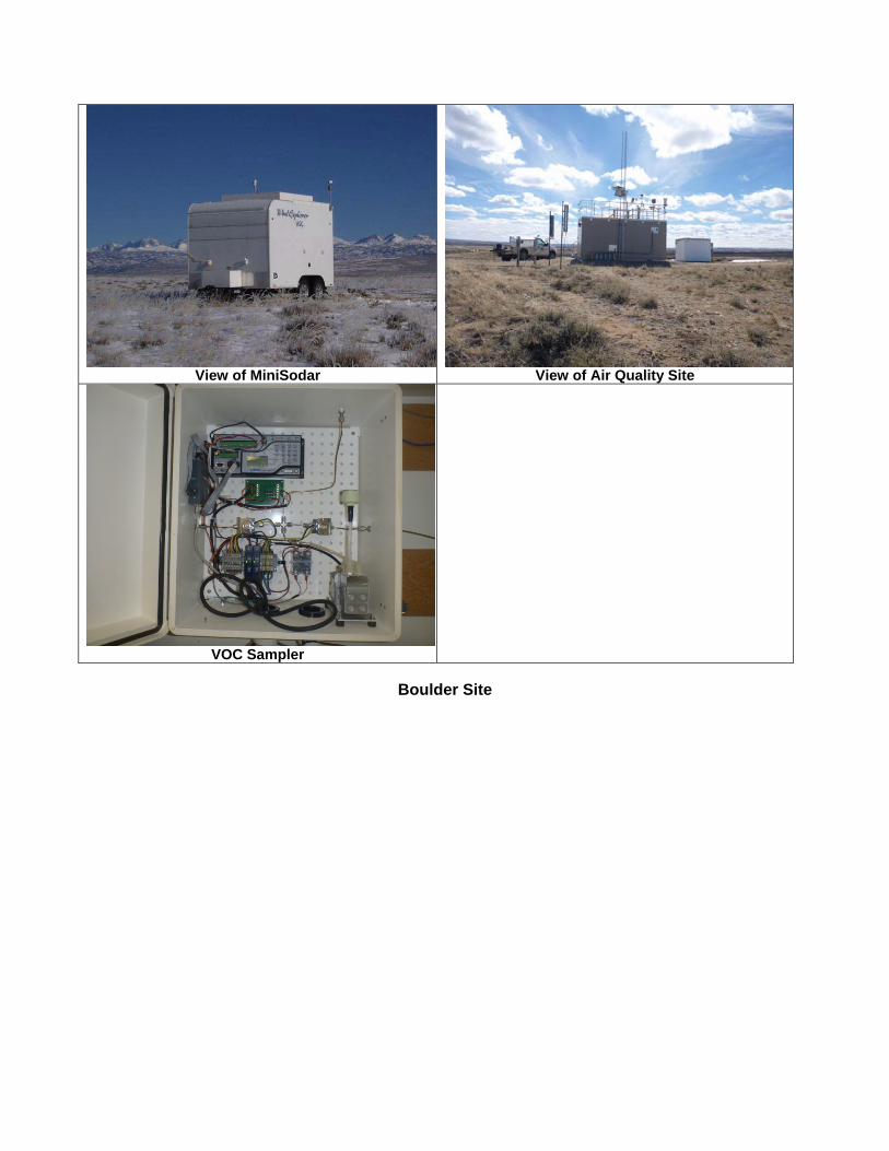
View of MiniSodar View of Air Quality Site
VOC Sampler
Boulder Site

Air Quality Site, View to North View to East
View to South View to West
Air Quality Site, with VOC Sampler on right
Big Piney VOC Sampling

View to North Air Quality Site, View to East
View to South View to West, with VOC Sampler
Air Quality Analyzers
Jonah Site

Monitoring Equipment, View to North View to East
View to South View to West
Jonah 2 Site
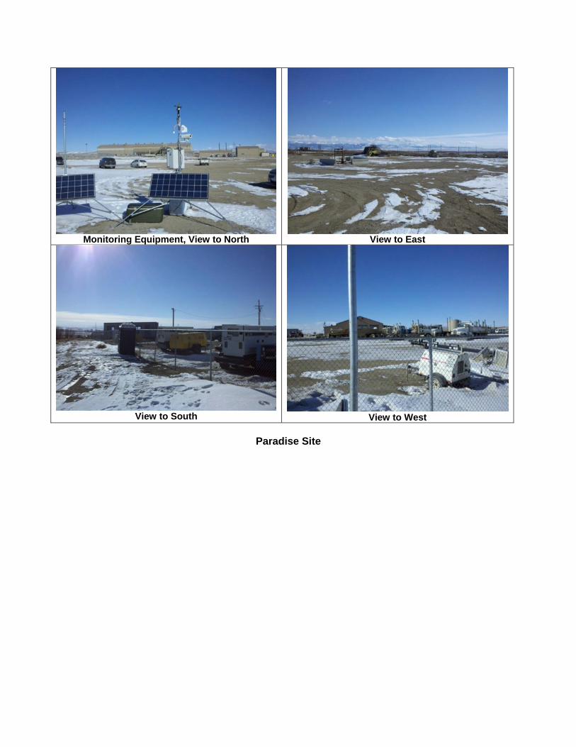
Monitoring Equipment, View to North
View to East
View to South View to West
Paradise Site
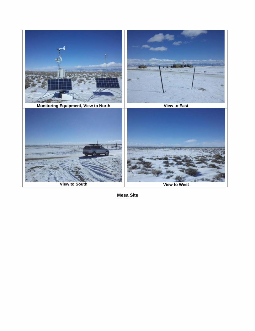
Monitoring Equipment, View to North
View to East
View to South View to West
Mesa Site
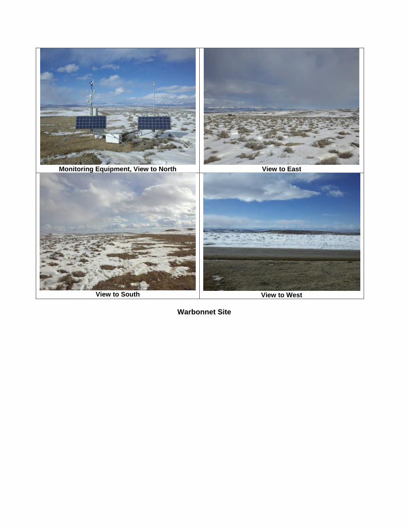
Monitoring Equipment, View to North
View to East
View to South View to West
Warbonnet Site

APPENDIX B
STANDARD OPERATING PROCEDURES

Page1of2
STANDARD OPERATING PROCEDURE
Title: 2B Model 202 Ozone Analyzer Calibration Procedures
Number: SOP 71 Page: 1 of 2
Revision Number: 1
Effective Date: 02/19/2013 02/17/2010 (Rev 0)
Approval: Date:
Concurred By:
Ozone Analyzer Calibration
1. If the analyzer is not already powered on and warmed up, turn it on and allow it to warm up for at least one hour to let internal temperature stabilize.
2. Log onto the data logger and add minutes to the ozone timer so that the channel is flagged.
Note the calibration start time in a log book.
3. Position the 2B Model 306 ozone standard near the station analyzer such that the calibration line reaches the sample inlet. Connect the sample inlet to the Teflon calibration line using a “T” with an atmospheric dump.
4. Connect the calibrator’s power cord adapter to the inverter that is powered by a 12V battery
inside the truck. Turn on the transfer standard and allow it to warm up. The calibrator display will read “warming up…” while doing so. When the indicated delT reading is within 1ºC, the display will read “Temperature Set Press Select”.
5. Adjust the Model 306 transfer standard to produce the zero and four span points. Record
raw and adjusted values on a datasheet.
6. The zero and four span points will create a slope and intercept. If the slope and intercept or the % differences have drifted significantly (>5%) from the previous calibration, enter the new slope and intercept into the data logger and recheck the zero and two span points to ensure a successful calibration.
7. Turn off standard and disconnect the sample line from the calibration line.
8. Before leaving the site ensure that the ozone timer minutes do not exceed five minutes.
9. To change the calibration parameters, select Cfg from the Main Menu:
Cfg Menu D/T Cal I/O Unt ← Cal Menu Z=-2
Use the rotary select switch to select and click on Cal. The following submenu with the values of the current calibration parameters will then appear:
S=1.01
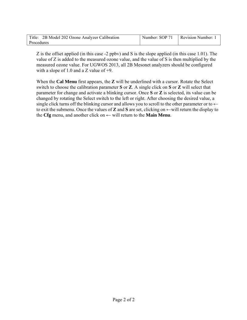
Page2of2
Title: 2B Model 202 Ozone Analyzer Calibration Procedures
Number: SOP 71 Revision Number: 1
Z is the offset applied (in this case -2 ppbv) and S is the slope applied (in this case 1.01). The value of Z is added to the measured ozone value, and the value of S is then multiplied by the measured ozone value. For UGWOS 2013, all 2B Mesonet analyzers should be configured with a slope of 1.0 and a Z value of +9. When the Cal Menu first appears, the Z will be underlined with a cursor. Rotate the Select switch to choose the calibration parameter S or Z. A single click on S or Z will select that parameter for change and activate a blinking cursor. Once S or Z is selected, its value can be changed by rotating the Select switch to the left or right. After choosing the desired value, a single click turns off the blinking cursor and allows you to scroll to the other parameter or to ← to exit the submenu. Once the values of Z and S are set, clicking on ←will return the display to the Cfg menu, and another click on ← will return to the Main Menu.

Page1of3
STANDARD OPERATING PROCEDURE
Title: 2B Model 202 Ozone Analyzer Troubleshooting and Maintenance Procedures
Number: SOP 72 Page: 1 of 3
Revision Number: 0
Effective Date: 01/06/2010
Approval: Date: Concurred By:
Ozone Analyzer Troubleshooting and Maintenance Procedures The only component that requires routine maintenance on the 2B Ozone analyzer is the ozone scrubber, which should be changed at least once every six months of operation. Other serviceable components include the lamp, air pump, and solenoid valve, all of which are easily replaced should they fail. Also, the inlet filter should be changed as conditions require. If the instrument fails to operate correctly, common problems can be identified and corrected using Table 1. If the problem cannot be corrected, the instrument may be returned to 2B Technologies for service.
Table 1 Troubleshooting the Ozone Analyzer
Problem/Symptom Likely Cause Corrective Action Instrument does not turn on
Power not connected properly or circuit breaker open. Power cable not connected to circuit board.
Check external power connection for reverse polarity or a short and wait a few minutes for the thermal circuit breaker to reset. Remove top cover and disconnect and reconnect power cable to circuit board.
Instrument turns on then powers off.
Burned out air pump. Remove top cover and unplug air pump. Turn instrument on; if it remains running, then the air pump motor is burned out and shorting. Replace air pump.
Display is blank or nonsense
Bad connection of display to circuit board.
Remove top cover and reconnect display to circuit board. Check solder connections to display.
Cell temperature reads low by several 10’s of degrees.
Absent or loose connection of temperature probe cable to circuit board.
Remove top cover and reattach connector to circuit board.
Readings are noisy with standard deviations greater than 2.0 ppbv.
Lamp output is weak. Excessive vibration.
Remove top cover and check lamp connection to circuit board. Run Lamp Test from menu. If photodiode voltage is less than 0.7 V, replace lamp. Provide additional vibration insulation for the instrument such

Page2of3
as a foam pad. Title: 2B Model 202 Ozone Analyzer Troubleshooting and Maintenance Procedures
Number: SOP 72 Revision Number: 0
Table 1 Continued
Troubleshooting the Ozone Analyzer Problem/Symptom Likely Cause Corrective Action
Readings are noisy with standard deviations greater than 2.0 ppbv.
Flow path contaminated. Clean flow path with methanol
Analog output is constant or does not track front display.
Cable not properly connected between analog output BNC and circuit board. Wrong scaling factor selected in menu.
Remove top cover and reconnect cable between analog output and circuit board. Check and reset analog output scaling factor in the Menu.
Select switch does not work.
Cable not properly connected between select switch and circuit board.
Remove top cover and reconnect select switch cable to circuit board.
Serial port does not work.
Cable not properly connected between serial port 9-pin connector and circuit board. Wrong serial cable used. Wrong baud rate selected.
Remove top cover and reconnect serial port cable to circuit board. A “straight through” serial cable is provided. Some data collection devices require a ”cross over” cable in which pins 1 and 3 are exchanged between the two ends of the cable. Use a “cross over cable or additional connector that switches pins 1 and 3. Make sure that the baud rate chosen in the menu matches the baud rate setting of your data acquisition program.
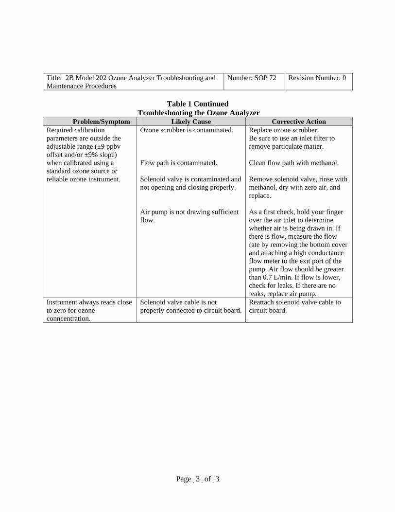
Page3of3
Title: 2B Model 202 Ozone Analyzer Troubleshooting and Maintenance Procedures
Number: SOP 72 Revision Number: 0
Table 1 Continued
Troubleshooting the Ozone Analyzer Problem/Symptom Likely Cause Corrective Action
Required calibration parameters are outside the adjustable range (±9 ppbv offset and/or ±9% slope) when calibrated using a standard ozone source or reliable ozone instrument.
Ozone scrubber is contaminated. Flow path is contaminated. Solenoid valve is contaminated and not opening and closing properly. Air pump is not drawing sufficient flow.
Replace ozone scrubber. Be sure to use an inlet filter to remove particulate matter. Clean flow path with methanol. Remove solenoid valve, rinse with methanol, dry with zero air, and replace. As a first check, hold your finger over the air inlet to determine whether air is being drawn in. If there is flow, measure the flow rate by removing the bottom cover and attaching a high conductance flow meter to the exit port of the pump. Air flow should be greater than 0.7 L/min. If flow is lower, check for leaks. If there are no leaks, replace air pump.
Instrument always reads close to zero for ozone conncentration.
Solenoid valve cable is not properly connected to circuit board.
Reattach solenoid valve cable to circuit board.

Page1of2
STANDARD OPERATING PROCEDURE
Title: 2B Model 306 Ozone Calibrator Calibration Procedures
Number: SOP 73 Page: 1 of 2
Revision Number: 1
Effective Date: 02/19/2013 02/17/2010 (Rev 0)
Approval: Date:
Concurred By:
Ozone Calibrator Calibration
1. Turn on the 306 calibrator and allow it to warm up for at least one hour prior to calibration in order to let internal temperature stabilize. The calibrator display will read “warming up…” while doing so. When the indicated delT reading is within 1ºC, the display will read “Temperature Set Press Select”. The calibration line that is used in the field should also be connected to the calibrator while it is warming up. This will allow the calibration line to be conditioned.
2. Turn on the transfer standard and allow it to warm up for at least one hour with the 306
calibrator.
3. Position the 2B Model 306 ozone standard near the transfer standard. Connect a sample inlet line of approximately three meters long to the sample inlet of the transfer standard. Connect this line to the calibration line using a T. A rotometer should be connected to the third port of the T to ensure sufficient overflow.
4. If sufficient overflow is not achieved, verify that the internal atmospheric dump of the 306
calibrator is capped.
5. Record calibrations start time in the logbook.
6. Adjust the Model 306 calibrator to produce the zero and four span points. Record the values on the datasheet.
7. Enter the new slope and intercept, calculated from the four span points, into the 2B 306 using the directions below.
To change the calibration parameters, select Cfg from the Main Menu: Cfg Menu D/T Cal I/O Unt ← Use the rotary select switch to select and click on Cal. The following submenu with the values of the current calibration parameters will then appear: Cal Menu Z=-2 S=1.01 Z is the offset applied (in this case -2 ppbv) and S is the slope applied (in this case 1.01).

Page2of2
Title: 2B Model 306 Ozone Calibrator Calibration Procedures
Number: SOP 73 Revision Number: 1
The value of Z is added to the measured ozone value, and the value of S is then multiplied by the measured ozone value. For example, if the instrument reads an average of 3 ppbv with the external scrubber in place, the value of Z should be set to –3. If after correction for the zero, the instrument consistently reads 2% low, the value of S should be set to 1.02.
When the Cal Menu first appears, the Z will be underlined with a cursor. Rotate the Select switch to choose the calibration parameter S or Z. A single click on S or Z will select that parameter for change and activate a blinking cursor. Once S or Z is selected, its value can be changed by rotating the Select switch to the left or right. After choosing the desired value, a single click turns off the blinking cursor and allows you to scroll to the other parameter or to ← to exit the submenu. Once the values of Z and S are set, clicking on ← will return the display to the Cfg menu, and another click on ← will return to the Main Menu.
8. Record the resultant calibration values on field calibration sheets.
9. If new values were entered into the 2B 306, perform an “as left” verification check starting
at Step 6.
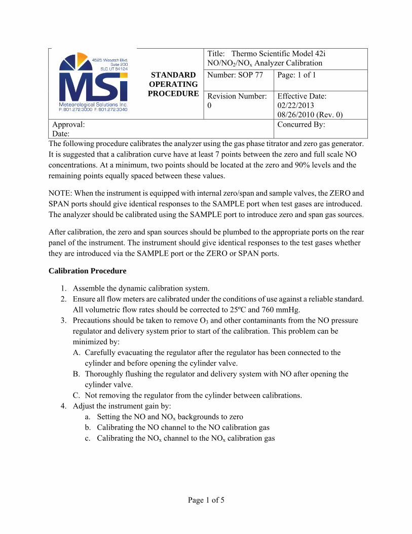
Page1of5
STANDARD OPERATING PROCEDURE
Title: Thermo Scientific Model 42i NO/NO2/NOx Analyzer Calibration
Number: SOP 77 Page: 1 of 1
Revision Number: 0
Effective Date: 02/22/2013 08/26/2010 (Rev. 0)
Approval: Date:
Concurred By:
The following procedure calibrates the analyzer using the gas phase titrator and zero gas generator. It is suggested that a calibration curve have at least 7 points between the zero and full scale NO concentrations. At a minimum, two points should be located at the zero and 90% levels and the remaining points equally spaced between these values.
NOTE: When the instrument is equipped with internal zero/span and sample valves, the ZERO and SPAN ports should give identical responses to the SAMPLE port when test gases are introduced. The analyzer should be calibrated using the SAMPLE port to introduce zero and span gas sources.
After calibration, the zero and span sources should be plumbed to the appropriate ports on the rear panel of the instrument. The instrument should give identical responses to the test gases whether they are introduced via the SAMPLE port or the ZERO or SPAN ports.
Calibration Procedure
1. Assemble the dynamic calibration system. 2. Ensure all flow meters are calibrated under the conditions of use against a reliable standard.
All volumetric flow rates should be corrected to 25ºC and 760 mmHg. 3. Precautions should be taken to remove O3 and other contaminants from the NO pressure
regulator and delivery system prior to start of the calibration. This problem can be minimized by: A. Carefully evacuating the regulator after the regulator has been connected to the
cylinder and before opening the cylinder valve. B. Thoroughly flushing the regulator and delivery system with NO after opening the
cylinder valve. C. Not removing the regulator from the cylinder between calibrations.
4. Adjust the instrument gain by: a. Setting the NO and NOx backgrounds to zero b. Calibrating the NO channel to the NO calibration gas c. Calibrating the NOx channel to the NOx calibration gas
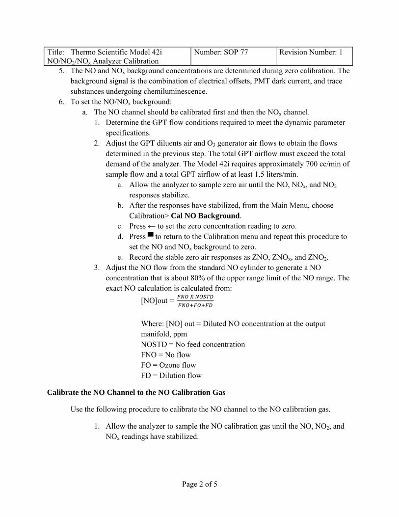
Page2of5
Title: Thermo Scientific Model 42i NO/NO2/NOx Analyzer Calibration
Number: SOP 77 Revision Number: 1
5. The NO and NOx background concentrations are determined during zero calibration. The background signal is the combination of electrical offsets, PMT dark current, and trace substances undergoing chemiluminescence.
6. To set the NO/NOx background: a. The NO channel should be calibrated first and then the NOx channel.
1. Determine the GPT flow conditions required to meet the dynamic parameter specifications.
2. Adjust the GPT diluents air and O3 generator air flows to obtain the flows determined in the previous step. The total GPT airflow must exceed the total demand of the analyzer. The Model 42i requires approximately 700 cc/min of sample flow and a total GPT airflow of at least 1.5 liters/min.
a. Allow the analyzer to sample zero air until the NO, NOx, and NO2 responses stabilize.
b. After the responses have stabilized, from the Main Menu, choose Calibration> Cal NO Background.
c. Press ← to set the zero concentration reading to zero. d. Press ▀ to return to the Calibration menu and repeat this procedure to
set the NO and NOx background to zero. e. Record the stable zero air responses as ZNO, ZNOx, and ZNO2.
3. Adjust the NO flow from the standard NO cylinder to generate a NO concentration that is about 80% of the upper range limit of the NO range. The exact NO calculation is calculated from:
[NO]out =
Where: [NO] out = Diluted NO concentration at the output manifold, ppm NOSTD = No feed concentration FNO = No flow FO = Ozone flow FD = Dilution flow
Calibrate the NO Channel to the NO Calibration Gas
Use the following procedure to calibrate the NO channel to the NO calibration gas.
1. Allow the analyzer to sample the NO calibration gas until the NO, NO2, and NOx readings have stabilized.
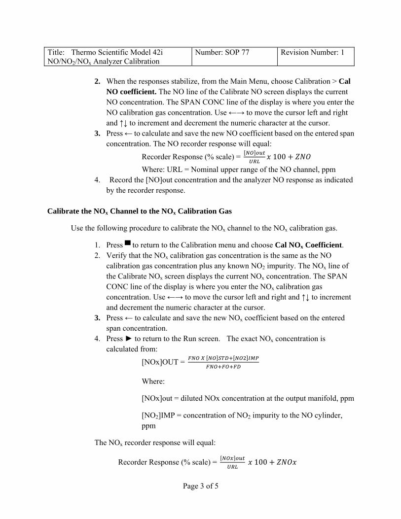
Page3of5
Title: Thermo Scientific Model 42i NO/NO2/NOx Analyzer Calibration
Number: SOP 77 Revision Number: 1
2. When the responses stabilize, from the Main Menu, choose Calibration > Cal
NO coefficient. The NO line of the Calibrate NO screen displays the current NO concentration. The SPAN CONC line of the display is where you enter the NO calibration gas concentration. Use ←→ to move the cursor left and right and ↑↓ to increment and decrement the numeric character at the cursor.
3. Press ← to calculate and save the new NO coefficient based on the entered span concentration. The NO recorder response will equal:
Recorder Response (% scale) = 100
Where: URL = Nominal upper range of the NO channel, ppm 4. Record the [NO]out concentration and the analyzer NO response as indicated
by the recorder response.
Calibrate the NOx Channel to the NOx Calibration Gas
Use the following procedure to calibrate the NOx channel to the NOx calibration gas.
1. Press ▀ to return to the Calibration menu and choose Cal NOx Coefficient. 2. Verify that the NOx calibration gas concentration is the same as the NO
calibration gas concentration plus any known NO2 impurity. The NOx line of the Calibrate NOx screen displays the current NOx concentration. The SPAN CONC line of the display is where you enter the NOx calibration gas concentration. Use ←→ to move the cursor left and right and ↑↓ to increment and decrement the numeric character at the cursor.
3. Press ← to calculate and save the new NOx coefficient based on the entered span concentration.
4. Press ► to return to the Run screen. The exact NOx concentration is calculated from:
[NOx]OUT =
Where:
[NOx]out = diluted NOx concentration at the output manifold, ppm
[NO2]IMP = concentration of NO2 impurity to the NO cylinder, ppm
The NOx recorder response will equal:
Recorder Response (% scale) = 100

Page4of5
Title: Thermo Scientific Model 42i NO/NO2/NOx Analyzer Calibration
Number: SOP 77 Revision Number: 1
Where:
URL = Nominal upper range limit of the NOx channel, ppm.
5. Record the NOx concentration and the analyzers NOx response.
Prepare the NO, NOx, and NO2 Calibration Curves
Use the following procedures to prepare the NO, NOx, and NO2 calibration curves.
1. Generate several additional NO and NOx concentrations by decreasing the FNO or increasing FD.
2. For each concentration generated, calculate the exact NO and NOx concentrations using the above equations for [NO]OUT and [NOx]OUT.
3. Record the NO and NOx responses.
4. Plot the analyzers responses versus the respective calculated NO and Nox concentrations and calculate the respective calibration curve.
5. Sample this NO concentration until the NO and NOx responses have stabilized, then measure and record the NO concentration as [NO]ORIG.
6. Adjust the GPT system to generate a NO concentration near 90% of the URL of the instrument range selected.
7. Adjust the O3 generator in the GPT system to generate sufficient O3 to produce a decrease in the NO concentration equivalent to about 80% if the URL of the NO2 range. The decrease must not exceed 90% of the NO concentration as determined in Steps 5 and 6 above.
8. When the analyzer responses stabilize, record the resultant NO concentration as [NO]REM.
9. From the Main Menu choose Calibration > Cal NO2 Coefficient. 10. Set the NO2 calibration gas concentration to reflect the sum of the following: the NO2
concentration generated by GPT, ([NO])ORIG-[NO]REM, and any NO2 impurity. Use ←→ to move the cursor left and right and ↑↓ to increment and decrement the numeric character at the cursor.
[NO2]OUT = ([NO]ORIG – [NO]REM) +
Where: [NO2]Out = diluted NO2 concentration at the output manifold, ppm [NO]ORIG = original NO concentration prior to addition of O3, ppm [NO]REM = NO concentration remaining after addition of O3, ppm.

Page5of5
Title: Thermo Scientific Model 42i NO/NO2/NOx Analyzer Calibration
Number: SOP 77 Revision Number: 0
11. Press ← to calculate and save the new NO2 coefficient based on the entered span
concentration. The analyzer does a one point NO2 span coefficient calculation, corrects the NO2 reading for converter efficiency, and then adds the corrected NO2 to the NO signal to give a corrected NOx signal. If the analyzer calculates a NO2 span coefficient of less than 0.96, either the entered NO2 concentration is incorrect, the converter is not being heated to the proper temperature, the instrument needs servicing, or the converter needs replacement. The recorder response will be as follows:
Recorder Response (% scale) = 100 2
Where: URL = Nominal upper range limit of the NO2 channel, ppm 12. Record the NO2 concentration and the analyzer’s NO2 response. 13. Maintaining the same FNO, FO, FD, adjust the ozone generator to obtain several other
concentrations of NO2 over the NO2 range. 14. Record the stable responses and plot the analyzer’s NO2 responses versus the
corresponding calculated (using the above equation for [NO2]OUT) concentrations and draw or calculate the NO2 calibration curve.

Approv
Connect filter is uthe outpuanalyzer,
Use the f
1. Ast
2. Wai
3. F4. F
careca
5. R
Use the f
1. G(Ure
2. Ais
3. Finin
R
WUZ[O
al:
the Model 4used, the caliut manifold i, and any oth
following proAllow sufficitabilize.
With the zeroir until a stabrom the Mairom the Calalibration. Pecommendedan be achiev
Record the st
following pro
Generate an oURL) of the espectively).
Allow the inss obtained. rom the Mai
ncrement/decnstrument. T
Recorder Res
Where: URL = UpperZ = RecorderO3]out = Oz
SOPR
49i to the maibration musis greater thaher flow dem
ocedure to aent time for
o air supply Oble responsein Menu choibration menress ► to red that it be aved by using able zero air
ocedure to a
ozone concenozone analy
. strument to s
in Menu chocrement the The recorder
sponse (% sc
r range limitr response wzone concent
1
STANDARDOPERATINGROCEDUR
anifold on tht be performan the total f
mand connec
Ze
adjust zero. the instrume
ON, but the e is obtainedoose Calibranu choose Ceturn to the Radjusted to ob
the zero offr response as
Spadjust span.
ntration stanyzer (such as
sample this o
oose Calibratknown span
r response w
cale) =
t of the Modith zero air, tration as det
1 of 1
D G
RE
Title: TAnalyzeNumber
Revisio0
Date:
e output of tmed through flow requiredcted to the m
ero Adjust
ent and the c
ozonator OF. ation. alibrate Zer
Run screen. Ibtain a recorfset capabilits Z.
pan Adjust
ndard of apprs, 0.4 or 0.8 p
ozone concen
tion > Calibn gas concen
will equal:
del 49i, ppm% scale termined by
Thermo Scieer Calibratior: SOP 79
on Number:
:
the ozonatorthis filter. Ed by the cali
manifold.
calibration p
FF, allow the
ro. Press ←If a strip chard of zero drty of the reco
roximately 8ppm for the
ntration stan
brate Span. ntration. Pres
y the calibrat
entific Modeon
Page: 1 o
Effective
Concurre
r. If an optionEnsure that thibration phot
photometer to
e instrument
to perform art recorder irift and/or zeorder.
80% of the u0.5 and 1.0
ndard until a
Use ↑ and ↓ss ← to calib
tion photome
el 49i Ozone
of 2
e Date: 12/6/
ed By:
nal sample lhe flow rate itometer,
o warm up a
t to sample z
a zero is used, it is ero noise. Th
upper range lppm ranges
stable respo
to brate the
eter, ppm
/2010
line into
and
zero
his
limit
onse

1 of 2
Title: Thermo Scientific Model 49i Ozone Analyzer Calibration
Number: SOP 79 Revision Number: 0
4. Record the ozone concentration as determined by the calibration photometer and the corresponding analyzer response.
Additional Concentration Standards
1. Generate several other ozone concentration standards (at least five others are recommended) over the scale range of the instrument.
2. For each ozone concentration standard, record the ozone concentration as determined by the calibration photometer and record the corresponding Model 49i analyzer response. If a Model 49i Primary Standard is being used as the calibration photometer, use the ozone concentration as determined by the photometer and not the value of the ozone level thumbwheel.
Calibration Curve
Use the following procedure to plot the calibration curve.
1. Plot the Model 49i Analyzer responses versus the corresponding ozone concentrations. 2. Connect the experimental points by using a straight line, preferably determined by linear
regression techniques. Points that lie more than ±4% from this line are an indication of an error in determining the calibration curve. The error may be due to a malfunction of the calibration photometer, or a malfunction of the analyzer being calibrated. The most likely malfunctions in both the analyzer and calibration photometer which can give non-linear results are leaks, a malfunctioning ozone scrubber, a dirty solenoid, or dirt in the optical system. The calibration curve is used to reduce subsequent ambient data.
Note: To generate data of the highest confidence, it is recommended that a multipoint calibration be performed every three months, any time major disassembly of components is performed, or any time the zero or span checks give results outside the limits described in “Periodic Zero and Span Checks” that follow.
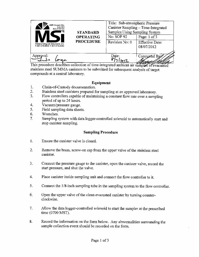

Page 2 of 3
Title: Sub-atmospheric Pressure Canister Sampling – Time-Integrated Samples Using Sampling System
Number: SOP 92 Revision Number: 0
9. The datalogger-controlled solenoid will stop the sample at the prescribed time
(1000 MST). 10. After the sample has stopped, retrieve the canister from the system. First, close the canister valve by turning clockwise and remove the flow controller. 11. Connect the pressure gauge to the canister, open the valve, record the stop pressure, close the valve, and remove the pressure gauge. 12. Replace the brass, screw-on cap onto the upper valve of the stainless steel canister. 13. Put the stainless steel canister back into the shipping carton. 14. Put the sample collection form into the shipping carton. 15. Bring the canister back to the Pinedale project base for shipment to the analytical
laboratory. 16. Ship to the analytical laboratory with chain-of-custody documentation.
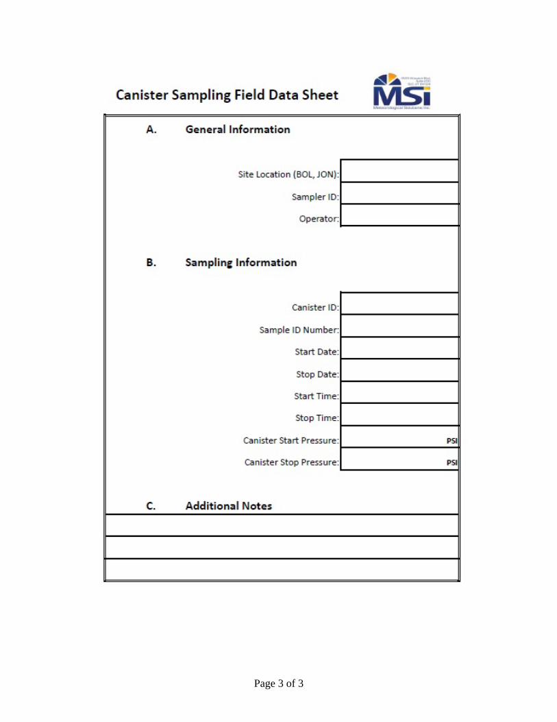
Page 3 of 3
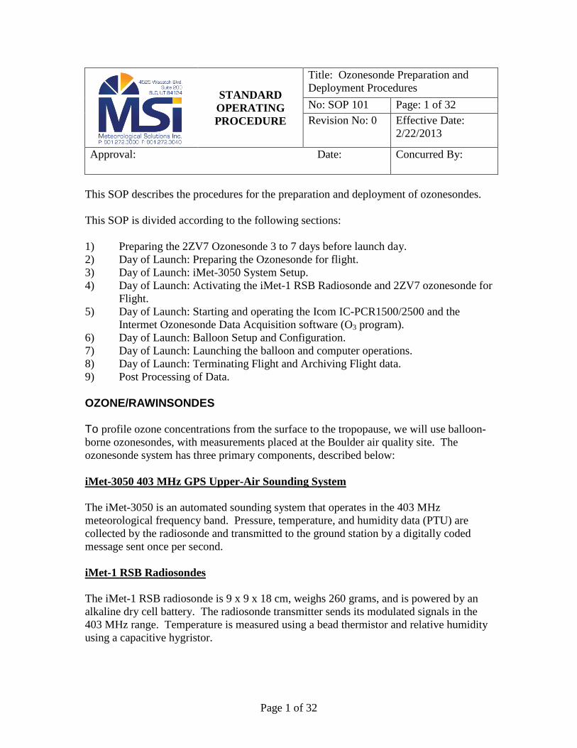
Page 1 of 32
STANDARD OPERATING PROCEDURE
Title: Ozonesonde Preparation and Deployment Procedures
No: SOP 101 Page: 1 of 32 Revision No: 0 Effective Date:
2/22/2013
Approval: Date: Concurred By:
This SOP describes the procedures for the preparation and deployment of ozonesondes. This SOP is divided according to the following sections: 1) Preparing the 2ZV7 Ozonesonde 3 to 7 days before launch day. 2) Day of Launch: Preparing the Ozonesonde for flight. 3) Day of Launch: iMet-3050 System Setup. 4) Day of Launch: Activating the iMet-1 RSB Radiosonde and 2ZV7 ozonesonde for
Flight. 5) Day of Launch: Starting and operating the Icom IC-PCR1500/2500 and the
Intermet Ozonesonde Data Acquisition software (O3 program). 6) Day of Launch: Balloon Setup and Configuration. 7) Day of Launch: Launching the balloon and computer operations. 8) Day of Launch: Terminating Flight and Archiving Flight data. 9) Post Processing of Data. OZONE/RAWINSONDES To profile ozone concentrations from the surface to the tropopause, we will use balloon-borne ozonesondes, with measurements placed at the Boulder air quality site. The ozonesonde system has three primary components, described below: iMet-3050 403 MHz GPS Upper-Air Sounding System The iMet-3050 is an automated sounding system that operates in the 403 MHz meteorological frequency band. Pressure, temperature, and humidity data (PTU) are collected by the radiosonde and transmitted to the ground station by a digitally coded message sent once per second. iMet-1 RSB Radiosondes The iMet-1 RSB radiosonde is 9 x 9 x 18 cm, weighs 260 grams, and is powered by an alkaline dry cell battery. The radiosonde transmitter sends its modulated signals in the 403 MHz range. Temperature is measured using a bead thermistor and relative humidity using a capacitive hygristor.

Page 2 of 32
Title: Ozonesonde Preparation and Deployment Procedures
Number: SOP 101 Rev. Number: 0
The iMet-1 RSB incorporates a low-noise integrated circuit GPS receiver. Winds aloft are calculated from the change in balloon position (determined from navaid) with time. Height is obtained directly from GPS positioning and, unlike older systems, pressure is now a derived parameter, calculated from the hydrostatic equation, using measured height, temperature, and humidity.
Accuracy (instrument specifications) Horizontal Wind Speed ± 1.0 ms-1 Horizontal Wind Direction Unknown Temperature ± 0.2° C Relative Humidity ±5.0%
Output Resolution Horizontal Wind Speed 0.1 m/s Horizontal Wind Direction 0.1° Temperature <0.01° C Relative Humidity <0.1%
EN-SCI Corporation 2ZV7-ECC Ozonesondes EN-SCI Corporation KZ-ECC ozonesonde system will be used in conjunction with the radiosonde package described above. Ozone is measured with an electrochemical concentration cell (ECC) ozonesonde coupled through an electronic interface to the radiosonde. The ECC ozonesonde is of a simple design consisting of a rigid mainframe on which is mounted a motor-driven Teflon/glass air sampling pump, a thermistor for measuring pump temperature, an ozone sensing ECC, and an electronics box containing interface circuitry which couple the ozone sensor to the radiosonde. The mainframe is mounted in a lightweight weatherproof polystyrene flight box that is taped and wired to the radiosonde during flight. The ozone-sensing cell is made of two bright platinum electrodes immersed in potassium iodide (KI) solutions of different concentrations contained in separate cathode and anode chambers. The chambers are linked with an ion bridge that, in addition to providing an ion pathway, retards mixing of the cathode and anode electrolytes thereby preserving their concentrations. The electrolytes also contain potassium bromide (KBr) and a buffer whose concentrations in each half-cell are the same.

Page 3 of 32
Title: Ozonesonde Preparation and Deployment Procedures
Number: SOP 101 Rev. Number: 0
The driving electromotive force for the cell, of approximately 0.13 V, is provided by the difference in potassium iodide concentrations in the two half cells. Sample air is forced through the ECC sensor by means of a non-reactive pump fabricated from TFE Teflon impregnated with glass fibers. The pump is designed to operate without ozone-destroying lubricants. Pumping efficiency for each pump varies from pump to pump and is also dependent on ambient air pressure. The sampling flow rate is calibrated at the factory and checked in the field before launch. The ECC ozone concentration calibration is also determined prior to launch. When ozone in air enters the sensor, iodine is formed in the cathode half cell according to the relation:
2KI + O3 + H2O → 2KOH + I2 + O2.
The cell converts the iodine to iodide according to:
I2 + 2e → 2I-
during which time two electrons flow in the cell’s external circuit. Measurement of the electron flow (i.e., the cell current), together with the rate at which ozone enters the cell per unit time, enables ozone concentrations in the sampled air to be derived from:
p3 = 4.307 x 10⁻³(im-ib)Tpt
where p3 is the ozone partial pressure in nanobars, im is the measured sensor output current in microamperes, ib is the sensor background current (i.e., the residual current emanating from the cell in the absence of ozone in the air) in microamperes, Tp is the pump temperature in Kelvin, and t is the time in seconds taken by the sonde gas sampling pump to force 100 ml of air through the sensor. As an integral part of the ozonesonde operations, the ozone analyzer readings at the Boulder site will provide ground-truth data.
Sensitivity 2-3 ppb by volume ozone in air
Response Time 15 seconds for 67% of change; 60 seconds for 85% of change
Noise less than 1% of full scale Estimated Measurement Uncertainty
less than ± 10% of indicated value

Page 4 of 32
Title: Ozonesonde Preparation and Deployment Procedures
Number: SOP 101 Rev. Number: 0
1) PREPARING THE 2ZV7 OZONESONDE 3 TO 7 DAYS BEFORE LAUNCH DAY.
Note 1. Preparation of the ozonesonde for flight should always be performed in a clean environment where smoking is prohibited; otherwise the performance of the instrument may be adversely affected. Note 2. Tubing connections to the sonde pump are made with pressure-fitted Teflon tubing. Should the fit appear to be too loose, enlarge the Teflon tube using a clean, awl-shaped tool of outside diameter slightly larger than the inside diameter of the tube. Use small strips of sand paper with which to grasp the Teflon tubing firmly when making or breaking pump connections.
Balloon-borne Model 2ZV7 ECC (Electrochemical Concentration Cell) Ozonesonde
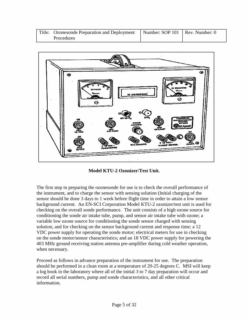
Page 5 of 32
Title: Ozonesonde Preparation and Deployment Procedures
Number: SOP 101 Rev. Number: 0
Model KTU-2 Ozonizer/Test Unit.
The first step in preparing the ozonesonde for use is to check the overall performance of the instrument, and to charge the sensor with sensing solution (Initial charging of the sensor should be done 3 days to 1 week before flight time in order to attain a low sensor background current. An EN-SCI Corporation Model KTU-2 ozonizer/test unit is used for checking on the overall sonde performance. The unit consists of a high ozone source for conditioning the sonde air intake tube, pump, and sensor air intake tube with ozone; a variable low ozone source for conditioning the sonde sensor charged with sensing solution, and for checking on the sensor background current and response time; a 12 VDC power supply for operating the sonde motor; electrical meters for use in checking on the sonde motor/sensor characteristics; and an 18 VDC power supply for powering the 403 MHz ground receiving station antenna pre-amplifier during cold weather operation, when necessary. Proceed as follows in advance preparation of the instrument for use. The preparation should be performed in a clean room at a temperature of 20-25 degrees C. MSI will keep a log book in the laboratory where all of the initial 3 to 7 day preparation will occur and record all serial numbers, pump and sonde characteristics, and all other critical information.

Page 6 of 32
Title: Ozonesonde Preparation and Deployment Procedures
Number: SOP 101 Rev. Number: 0
(a) Remove the sonde from its polystyrene flight box and connect the Teflon air intake tube packed with the instrument to the sonde pump. (b) Connect the ozonesonde battery power leads to the ozonizer/test unit's 12 VDC output power supply terminals. Pull the ECC sensors’ air intake tube away from the pump. Next, insert the pump air intake tube into the NO-LO OZONE port of the unit. With all ozonizer/test unit switches, except the 18 VDC power supply switch and the UV lamp switch, turned ON, operate the sonde pump for 10 minutes (during which time clean, ozone-free air will be passed through the pump. After the 10-minute interval, check the current drawn by the sonde ( pump motor and V7 interface board) at about 12.3 VDC. The current should be less than 100 mA. (The current drawn by the interface board is about 8 mA.) If the current is larger, the fit between the piston and cylinder may be too tight and may cause excessive frictional heating. Continue operating the pump for an additional 20 minutes to see if the current decreases. If it does not, take remedial action as outlined in Appendix C. A properly adjusted pump will draw less than 90 mA of current, and develop at least 50 cm (*20 inches) of Hg pressure and 45 cm (*18 inches) of Hg vacuum. Measure the pressure and vacuum developed by the pump with a pressure/vacuum gauge. (c) With proper pump performance attained, remove the sonde air intake tube from the NO-LO OZONE port of the ozonizer/test unit, and insert it snugly into the HI OZONE port of the unit. (The connection must be snug since the sonde pump draws highly ozonized air from the unit.) Next, remove the top plug with air intake tube from the sensor cathode chamber, and re-connect the air intake tube to the pump. Now turn OFF the AIR PUMP switch, but turn ON the UV LAMP switch, and pull out the OZONE CONTROL tube as far as possible out of the chassis. Conditioning of the sonde Teflon tubing, pump, and sensor air intake tube (but not the sensor cathode chamber) with high ozone now begins. Blue light visible through a hole in the front of the OZONE CONTROL tube indicates that the UV lamp is ON. During the conditioning, avoid direct breathing of the ozonized air coming out of the sensor air intake tube. Condition with high ozone for 30 minutes. (d) After conditioning with high ozone is completed, push the OZONE CONTROL tube as far as possible into the ozonizer/test unit chassis, turn ON the AIR PUMP switch, and withdraw the sonde air intake tube from the HI OZONE port and insert it into the NO-LO OZONE port. Ozone-free air will now be passing through the pump and sensor air intake tube to flush out the ozone. Continue flushing for 3-5 minutes. (e) Now unplug the sensor leads from the sonde electronic interface board, and plug them into the sensor cable connector of the ozonizer/test unit. Then charge the sensor with sensing solution as follows:
Page 7 of 32
Title: Ozonesonde Preparation and Deployment Procedures
Number: SOP 101 Rev. Number: 0
The sensor cathode must always be charged first to allow cathode solution to permeate the sensor's ion bridge. Using a Teflon-tipped syringe especially reserved for use with cathode sensing solution, inject 3.0 ml of the solution into the sensor cathode chamber. This is the chamber containing the large platinum screen. When re-installing the top plug of the cathode, make sure that the air intake tube is correctly centered within the cathode chamber by inserting the tube carefully over a thin Teflon rod projecting out of the bottom plug of the sensor cathode chamber. Rinse the syringe with distilled water prior to storage. Note: Do not attempt to fill or empty the sensor cathode through the short air exhaust tube of the cathode chamber top plug; otherwise, the platinum screen may be damaged (distorted), leading to sensor malfunction. Next, after waiting 2 minutes to allow the cathode sensing solution to permeate the sensor’s ion bridge, use a syringe especially reserved for dispensing anode solution to inject 1.5 ml anode sensing solution into the sensor anode chamber. Rinse the syringe with distilled water prior to storage. (f) After charging the sensor with solution, run the sonde on ozone-free air for 5-10 minutes. The sensor current, as observed on the ozonizer/test unit microammeter should be low, 0.5 micro A or less. Now set the ozonizer/test unit OZONE CONTROL tube position for a low ozone output, one that produces a sensor current of 5 micro A. Continue input of ozonized air into the sensor for 10 minutes while periodically adjusting the OZONE CONTROL tube position as needed. At the end of the 10-minute interval, abruptly push the OZONE CONTROL tube as far as possible into the ozonizer/test unit front panel to begin the flow of ozone-free air through the sensor. Read the microammeter current 1 minute later; it should then have decreased from the original value of 5 micro Amps to 1.5 micro Amps or less, indicating satisfactory ECC sensor performance. (g) Continue running the sonde on ozone-free air for 10 minutes. Then turn off all ozonizer/test unit switches, and disconnect the sonde from the unit. Prior to storage of the sonde until flight day, add 2.5 ml cathode sensing solution to the sensor cathode chamber to fill it about 3/4 full. Re-insert the sensor cathode chamber air intake tube into the sensor, and store the sonde in a dark, clean-air environment at a temperature of 20-25deg C until the day of the flight. IMPORTANT! Prior to storage, also, short the ECC sensor leads together with a shorting plug. This will allow a sensor cleaning action to proceed during storage. (Do not re-plug the sensor into the sonde's electronic interface board for storage since the unpowered board's input impedance may be high, and proper sensor cleaning action would not proceed.)
Page 8 of 32
Title: Ozonesonde Preparation and Deployment Procedures
Number: SOP 101 Rev. Number: 0
2) DAY OF LAUNCH: PREPARING THE OZONESONDE FOR FLIGHT. The preparation should be conducted in a clean room at a temperature of 20-25 degrees Celsius. MSI will keep a log book on-site and record all serial numbers, sonde characteristics, and all other critical information. (a) Remove the top plug from the sensor cathode chamber and remove all solution from the chamber. Now rinse the chamber by injecting into it 3.0 ml fresh cathode solution, then removing the solution completely from the chamber. Finally, refill the chamber with 3.0 ml cathode solution. (Note: For soundings of duration less than 3-4 hours, made primarily to measure tropospheric ozone, 2.5 ml cathode sensing solution may be used, instead. Sensor response time will then be improved.) Replace the top plug. Next, remove the top plug from the sensor anode chamber and remove all anode solution from the chamber. Re-fill the chamber with 1.5 ml of fresh anode solution. Replace the anode plug. (b) Connect the ECC sonde motor and sensor leads to the ozonizer/test unit, and insert the sonde air intake tube into the NO-LO OZONE port of the unit to a distance of about 7 cm. Set the controls so that ozone-free air passes through the air pump and sensor. Next, turn on the UV LAMP switch to warm up the lamp. Continue passing ozone-free air through the sensor for a total of 10 minutes. At the end of the 10-minute interval, record the sensor background current (which generally should be less than 0.05 µA). Save this information as part of your raw data file (e.g., ib1 = 0.05 µA). (c) Pull the OZONE CONTROL tube out of the ozonizer/test unit a distance such that, after several minutes, the sonde sensor output current becomes approximately 5 µA. Continue passing an equivalent of 5 µA ozone current through the sensor for a total of 10 minutes. Periodically adjust the position of the OZONE CONTROL tube so that at the end of the 10-minute interval the ECC sensor current is exactly 5.0 µA. (d) Check the ECC sensor response time as follows: Using a stopwatch, at time t = 0 quickly push the ozonizer/test unit OZONE CONTROL tube all the way into the instrument chassis and turn the UV LAMP switch OFF. As the ECC sensor current continues to fall, record the current for times t = 0, 0.5, 1, 3, 5 and 10 minutes as shown in the example on the following page giving typical measurement results at 20°C. Record also the room temperature at which this test was performed. Save all the information as part of the raw data file.

Page 9 of 32
Title: Ozonesonde Preparation and Deployment Procedures
Number: SOP 101 Rev. Number: 0
Sensor response time R, is satisfactory if: R = 100[(im(t = 0) - im(t = 1))/im(t = 0)] ≥ 80%.
t Sensor Current, 0 min. 5.00 µA 0.5 1.61
1 0.82
3 0.25
5 0.20
10 0.10 For the above example, R = 83.6%. Sensor response time becomes faster as sensor temperature increases. (e) After the sensor response time check is completed, continue running the ozonesonde on ozone-free air for another 10-15 minutes. During this time, re-connect the ECC sensor leads to the V7 interface board. Connect the ozonesonde to the InterMet radiosonde. Activate your data acquisition system for operation in the “Calibration” mode to begin receiving and recording the radiosonde and ozonesonde data by computer. (See Appendix E for configuration of the data acquisition system). This procedure will enable you to check for satisfactory performance of the ozone-radiosonde instrument package as a whole. At this stage, the ozonesonde should still be operated without its flight box at a room temperature of 20-25 deg C, and powered by the ozonizer/test unit's 12 VDC power supply. Power the InterMet radiosonde with an auxiliary 6 V battery power supply. As the sonde is continuing to be run on ozone-free air, perform a sonde pump air flow rate according to instructions given in Appendix D (Due to a miscalibrated bubble meter device, this Appendix in the manual will not be followed. MSI will use a certified Alltech mass flow meter to check the pump flow rate). Check to insure that the pump motor voltage is about 12.3 volts. Record the pump motor voltage and current (which should be less than about 110 mA). Record also the pump air flow rate and the room temperature, and save all information as part of the raw data file. Now enter into your computer raw data file all pertinent ozonesonde and radiosonde calibration data, instrument serial numbers, station name, release date, etc. At the end of the final 10-minute ozone-zero air conditioning period, record in the raw data file, also, the ECC sensor background current (ib2) which should generally be less than about 0.1 micro A.

Page 10 of 32
Title: Ozonesonde Preparation and Deployment Procedures
Number: SOP 101 Rev. Number: 0
(f) Turn off power to the ozonizer/test unit. (By this time, inflation of the flight balloon and preparation of the flight train should have been completed.) Install the ECC sonde into its flight box together with the sonde pump motor battery, but do not activate the battery. Activate the radiosonde by plugging the leads connector of the 2-cell lithium battery pack, located within the radiosonde, into its mating connector mounted on the radiosonde electronics board. Tape the radiosonde to the ozone instrument flight box (see Appendix F for configuring the instrument package for flight). Affix a return address/reward notice to the cover so that the instrument could be returned to your laboratory should someone recover it. (g) Carry the ozonesonde package outdoors, and suspend it from a pole (or set it on a platform) at a height of about 1.5 meters above the ground, with the sonde air intake tube pointing into the wind. Connect the sonde pump motor battery leads to begin ECC ozonesonde operation. Activate the 403 MHz ground receiving equipment for operation in the “Surface Ozone Measurement” mode to measure and record surface ozone data for 10 minutes. In very warm weather, the surface ozone measurement should be made with the cover off the sonde weatherproof box to prevent excessive heat build-up within the box. Tape the cover on to the box prior to instrument release. 3) DAY OF LAUNCH: IMET-3050 SYSTEM SETUP. The iMet-3050 403 MHz GPS Upper-Air Sounding System Components
Item Description InterMet Part
Number N/S CD with Software, Drivers, and Documentation 693,050
1 403 MHz Antenna with Base and Tripod 100,244 2 LNA to 403 MHz Antenna Cable 597,426 3 403 MHz LNA 900,002 4 403 MHz Cable 597,444 5 GPS Cable (Optional) 597,443 6 AC Power Cable Varies 7 DC Power Supply 501,046 8 GPS Re-Radiator (Optional) 100,185 9 GPS Re-Radiator Cable (Optional) 597,422 10 iMet-3050 Meteorological Processor 100,413 11 USB Cable 597,049 12 System Computer Power Cord Optional / Varies 13 System Computer Optional / Varies
N/S Cable Reel for 403 MHz Cable / GPS Cable 490,005

Page 11 of 32
Title: Ozonesonde Preparation and Deployment Procedures
Number: SOP 101 Rev. Number: 0
The iMet-3050 403 MHz GPS Upper-Air Sounding System Components – (Continued)
Item Description InterMet Part
Number N/S UPS Optional / Varies N/S Transportation Case for System Cables (Optional) 300,020 N/S Transportation Case for System, Re-Rad, LNA
(Optional) 300,021
N/S Transportation Case for Tripod Unit (Optional) 300,022 N/S Balloon Inflation Kit 100,438
a) Setup Antenna Unit outside
• Tripod may be placed up to 30 m away from iMet-3050 MP location • High and clear areas provide for the best reception of radiosonde data • Avoid valleys, buildings, trucks, and electrical wires • Adjust tripod legs to orientate the 403 MHz Antenna to approximately
vertical
M403 MHz Antenna Unit with Cables attached.
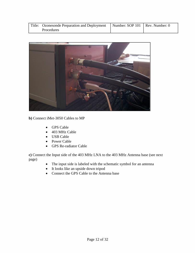
Page 12 of 32
Title: Ozonesonde Preparation and Deployment Procedures
Number: SOP 101 Rev. Number: 0
b) Connect iMet-3050 Cables to MP
• GPS Cable • 403 MHz Cable • USB Cable • Power Cable • GPS Re-radiator Cable
c) Connect the Input side of the 403 MHz LNA to the 403 MHz Antenna base (see next page)
• The input side is labeled with the schematic symbol for an antenna • It looks like an upside down tripod • Connect the GPS Cable to the Antenna base
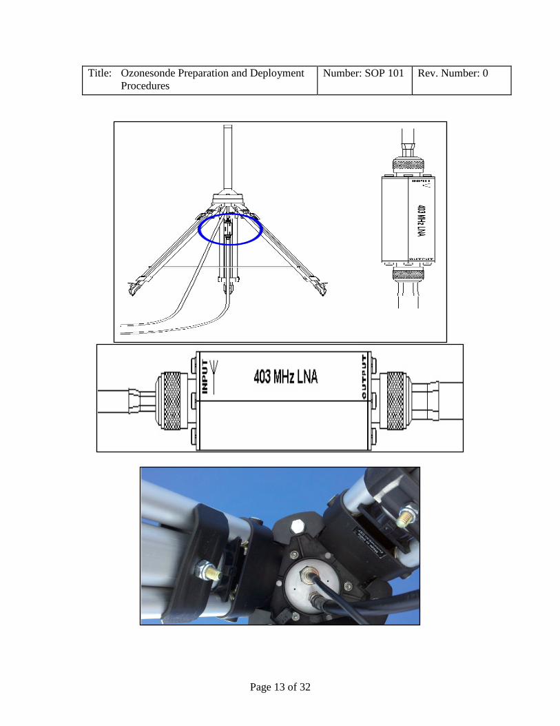
Page 13 of 32
Title: Ozonesonde Preparation and Deployment Procedures
Number: SOP 101 Rev. Number: 0
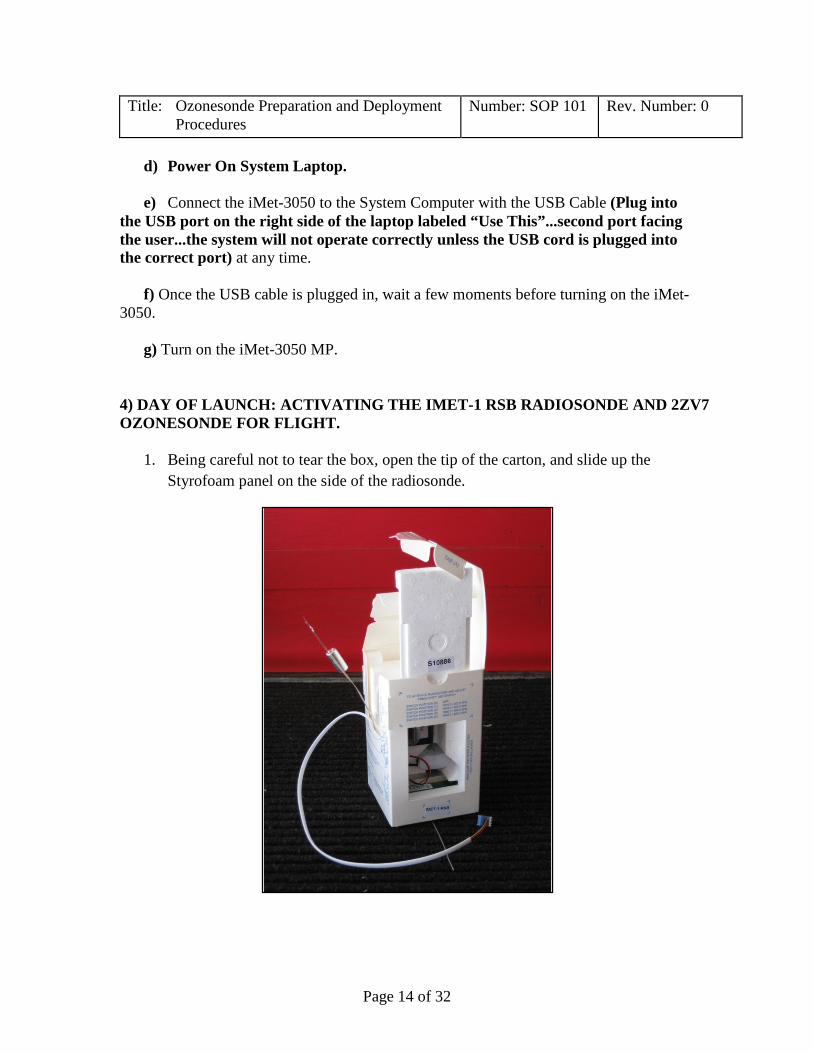
Page 14 of 32
Title: Ozonesonde Preparation and Deployment Procedures
Number: SOP 101 Rev. Number: 0
d) Power On System Laptop.
e) Connect the iMet-3050 to the System Computer with the USB Cable (Plug into
the USB port on the right side of the laptop labeled “Use This”...second port facing the user...the system will not operate correctly unless the USB cord is plugged into the correct port) at any time.
f) Once the USB cable is plugged in, wait a few moments before turning on the iMet-
3050.
g) Turn on the iMet-3050 MP. 4) DAY OF LAUNCH: ACTIVATING THE IMET-1 RSB RADIOSONDE AND 2ZV7 OZONESONDE FOR FLIGHT.
1. Being careful not to tear the box, open the tip of the carton, and slide up the Styrofoam panel on the side of the radiosonde.
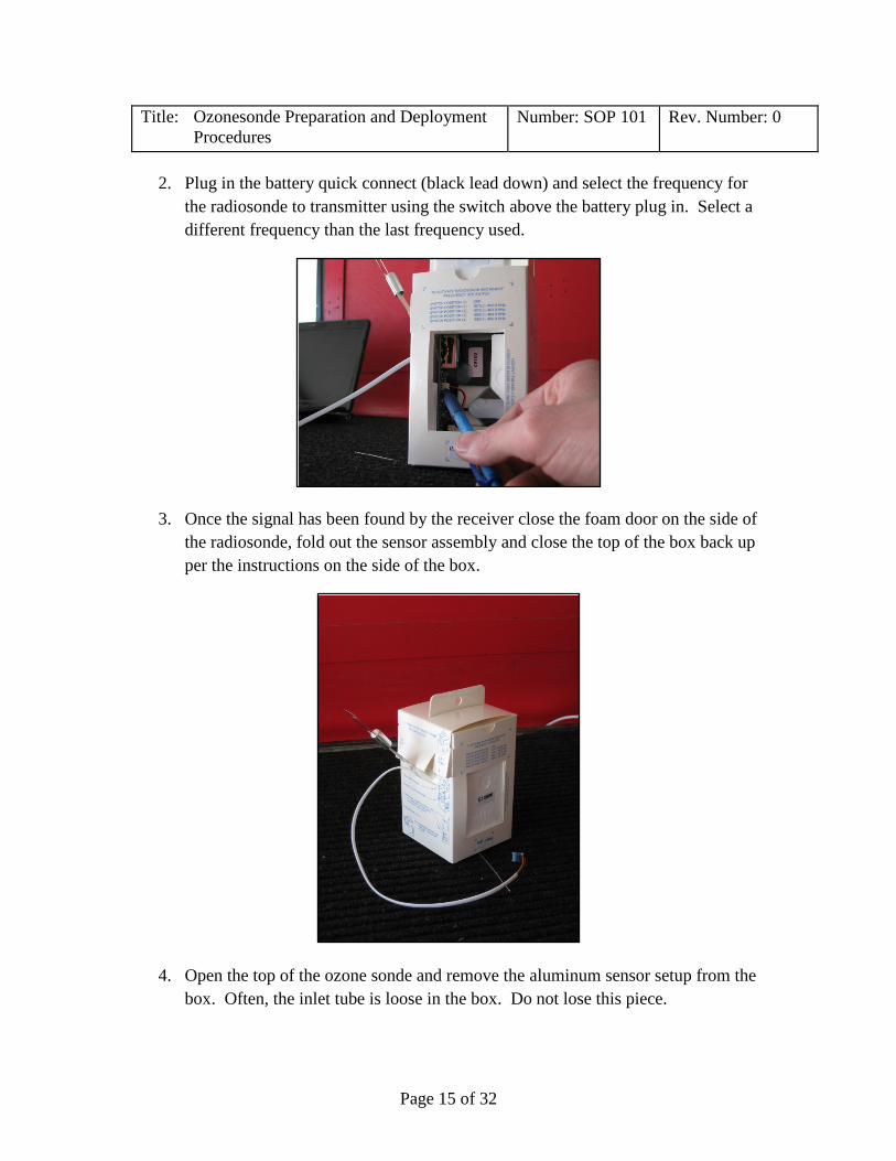
Page 15 of 32
Title: Ozonesonde Preparation and Deployment Procedures
Number: SOP 101 Rev. Number: 0
2. Plug in the battery quick connect (black lead down) and select the frequency for
the radiosonde to transmitter using the switch above the battery plug in. Select a different frequency than the last frequency used.
3. Once the signal has been found by the receiver close the foam door on the side of the radiosonde, fold out the sensor assembly and close the top of the box back up per the instructions on the side of the box.
4. Open the top of the ozone sonde and remove the aluminum sensor setup from the box. Often, the inlet tube is loose in the box. Do not lose this piece.
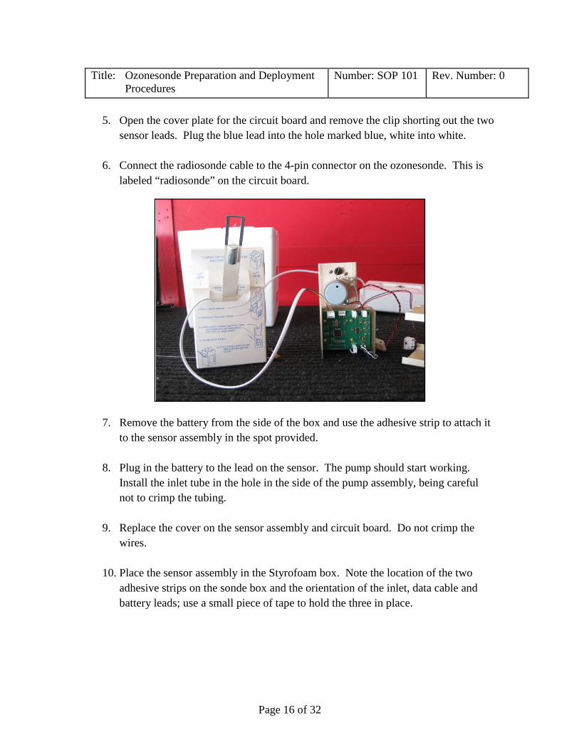
Page 16 of 32
Title: Ozonesonde Preparation and Deployment Procedures
Number: SOP 101 Rev. Number: 0
5. Open the cover plate for the circuit board and remove the clip shorting out the two
sensor leads. Plug the blue lead into the hole marked blue, white into white.
6. Connect the radiosonde cable to the 4-pin connector on the ozonesonde. This is labeled “radiosonde” on the circuit board.
7. Remove the battery from the side of the box and use the adhesive strip to attach it to the sensor assembly in the spot provided.
8. Plug in the battery to the lead on the sensor. The pump should start working. Install the inlet tube in the hole in the side of the pump assembly, being careful not to crimp the tubing.
9. Replace the cover on the sensor assembly and circuit board. Do not crimp the wires.
10. Place the sensor assembly in the Styrofoam box. Note the location of the two adhesive strips on the sonde box and the orientation of the inlet, data cable and battery leads; use a small piece of tape to hold the three in place.
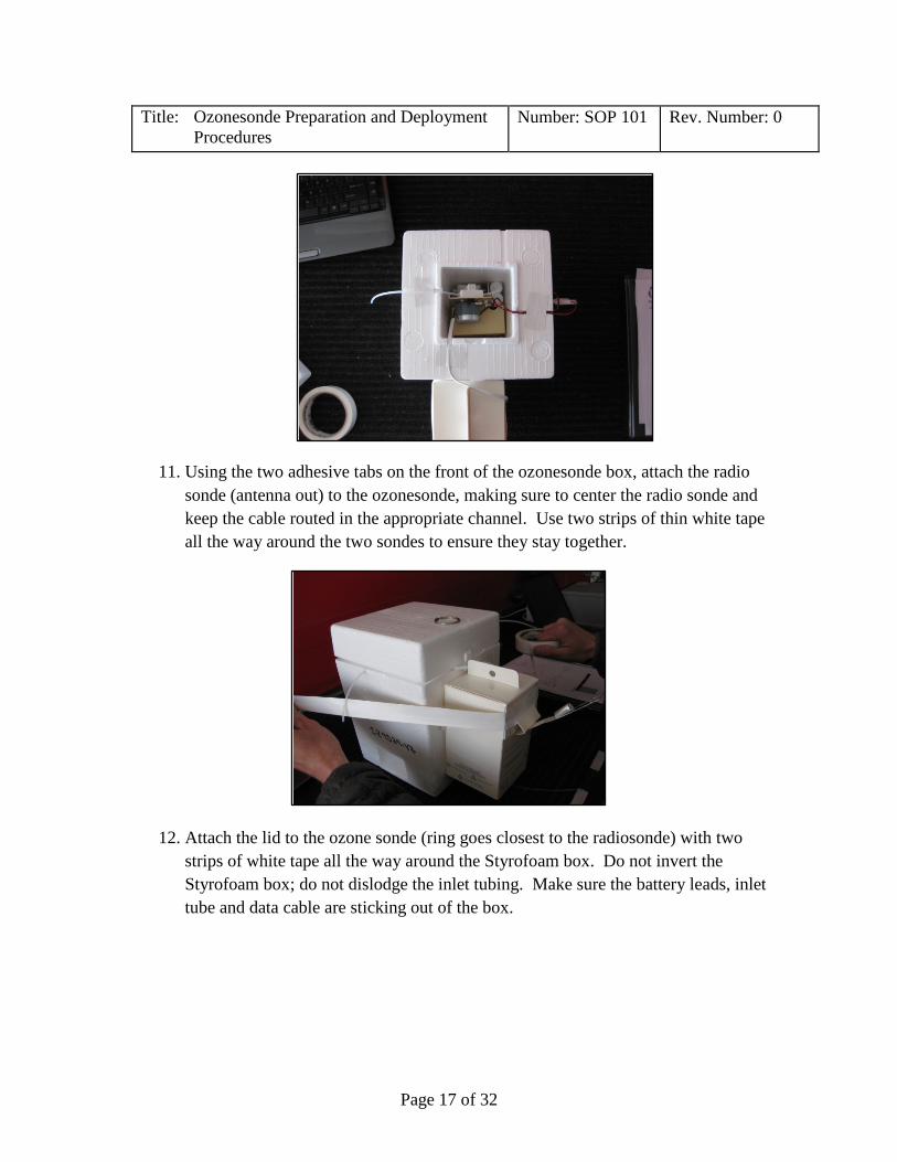
Page 17 of 32
Title: Ozonesonde Preparation and Deployment Procedures
Number: SOP 101 Rev. Number: 0
11. Using the two adhesive tabs on the front of the ozonesonde box, attach the radio sonde (antenna out) to the ozonesonde, making sure to center the radio sonde and keep the cable routed in the appropriate channel. Use two strips of thin white tape all the way around the two sondes to ensure they stay together.
12. Attach the lid to the ozone sonde (ring goes closest to the radiosonde) with two strips of white tape all the way around the Styrofoam box. Do not invert the Styrofoam box; do not dislodge the inlet tubing. Make sure the battery leads, inlet tube and data cable are sticking out of the box.

Page 18 of 32
Title: Ozonesonde Preparation and Deployment Procedures
Number: SOP 101 Rev. Number: 0
13. Place the sondes outside prior to launch on a clean, level spot.
14. Verify that the data the sondes are collecting is being received by the base station.
5) DAY OF LAUNCH: STARTING AND OPERATING THE ICOM IC-PCR1500/2500 AND THE INTERMET OZONESONDE DATA ACQUISITION SOFTWARE (O3 PROGRAM). The Icom IC-PCR1500/2500 software is required to control the receiver within the iMet-3050.
a. Start the Icom PC-PCR1500/2500 software by using the desktop icon.
b. Once the software has initialized, the Icom Toolbar will open and display.

Page 19 of 32
Title: Ozonesonde Preparation and Deployment
Procedures Number: SOP 101 Rev. Number: 0
Icom Toolbar Top
c. Click the [Power] icon on the Toolbar to connect the control software and the receiver.
d. Click the [Compo] button to open the Component Screen.
e. In the Tuning Panel window, press the Bank [Up]/[Down] buttons until the Bank reads “00: IMS Uses”.
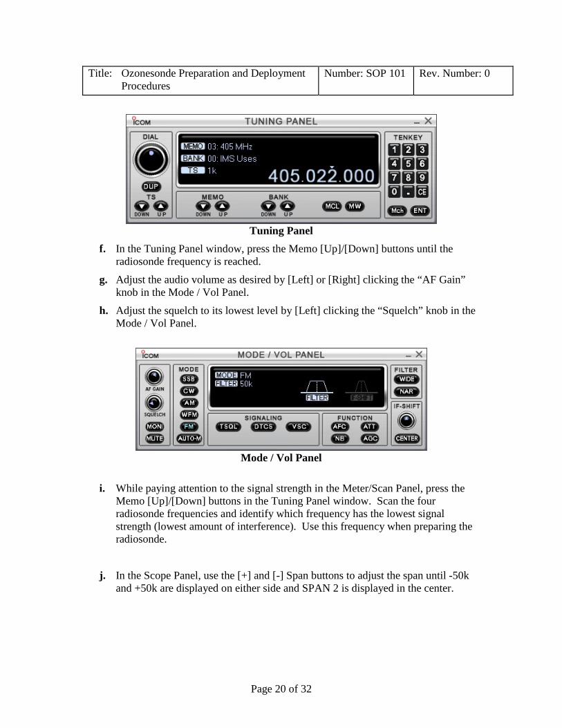
Page 20 of 32
Title: Ozonesonde Preparation and Deployment Procedures
Number: SOP 101 Rev. Number: 0
Tuning Panel
f. In the Tuning Panel window, press the Memo [Up]/[Down] buttons until the radiosonde frequency is reached.
g. Adjust the audio volume as desired by [Left] or [Right] clicking the “AF Gain” knob in the Mode / Vol Panel.
h. Adjust the squelch to its lowest level by [Left] clicking the “Squelch” knob in the Mode / Vol Panel.
Mode / Vol Panel
i. While paying attention to the signal strength in the Meter/Scan Panel, press the Memo [Up]/[Down] buttons in the Tuning Panel window. Scan the four radiosonde frequencies and identify which frequency has the lowest signal strength (lowest amount of interference). Use this frequency when preparing the radiosonde.
j. In the Scope Panel, use the [+] and [-] Span buttons to adjust the span until -50k and +50k are displayed on either side and SPAN 2 is displayed in the center.

Page 21 of 32
Title: Ozonesonde Preparation and Deployment Procedures
Number: SOP 101 Rev. Number: 0
Scope Panel
k. Using the Dial in the Tuning Panel, [Left] or [Right] click to fine-tune the receiver frequency such that the Red line in the Scope Panel is approximately centered between the twin peaks.
l. The signal strength in the Meter/Scan panel should now show full signal strength. If it does not, re-check the security of all the RF connectors. Also, verify that the LNA feels warmer to the touch.
Meter / Scan Panel
Setup of the Icom IC-PCR1500/2500 is complete. InterMet Ozonesonde Data Acquisition software (O3 program)
1) Open the “O3” program.
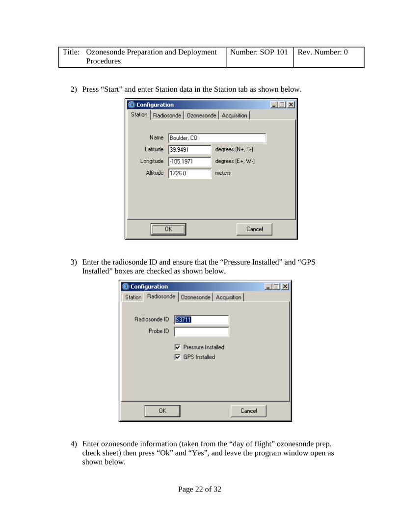
Page 22 of 32
Title: Ozonesonde Preparation and Deployment Procedures
Number: SOP 101 Rev. Number: 0
2) Press “Start” and enter Station data in the Station tab as shown below.
3) Enter the radiosonde ID and ensure that the “Pressure Installed” and “GPS Installed” boxes are checked as shown below.
4) Enter ozonesonde information (taken from the “day of flight” ozonesonde prep. check sheet) then press “Ok” and “Yes”, and leave the program window open as shown below.

Page 23 of 32
Title: Ozonesonde Preparation and Deployment Procedures
Number: SOP 101 Rev. Number: 0
5) The “O3” software will show signals being received from not only the Ozonesonde but also the radiosonde by blinking green lights in the lower right hand corners of the “Radiosonde”, “GPS”, and “Ozonesonde” labels under the “Surface Data” screen.
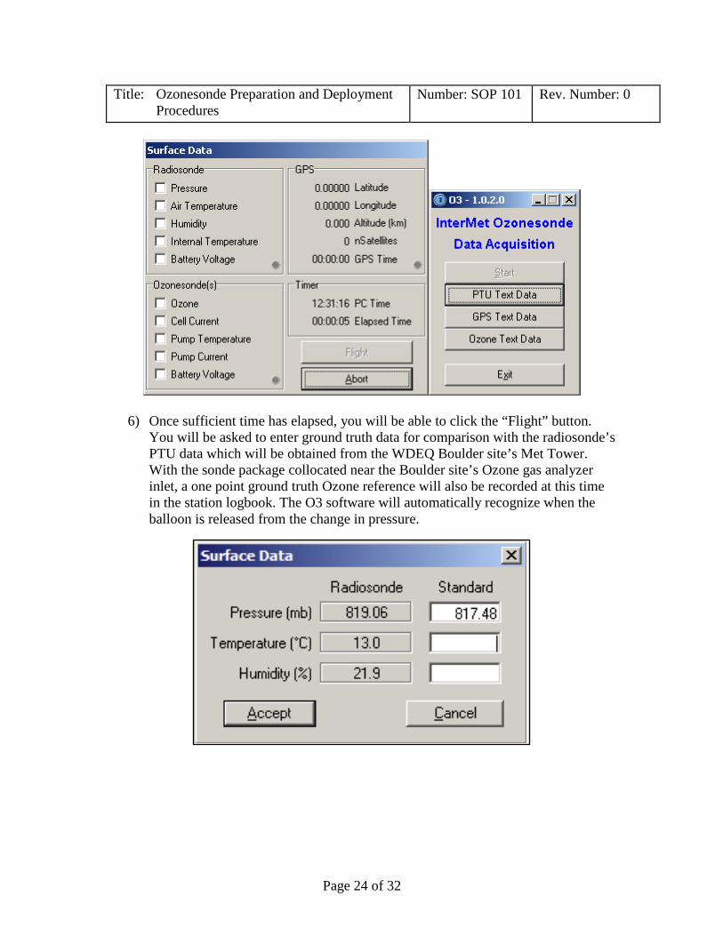
Page 24 of 32
Title: Ozonesonde Preparation and Deployment Procedures
Number: SOP 101 Rev. Number: 0
6) Once sufficient time has elapsed, you will be able to click the “Flight” button. You will be asked to enter ground truth data for comparison with the radiosonde’s PTU data which will be obtained from the WDEQ Boulder site’s Met Tower. With the sonde package collocated near the Boulder site’s Ozone gas analyzer inlet, a one point ground truth Ozone reference will also be recorded at this time in the station logbook. The O3 software will automatically recognize when the balloon is released from the change in pressure.

Page 25 of 32
Title: Ozonesonde Preparation and Deployment Procedures
Number: SOP 101 Rev. Number: 0
6) DAY OF LAUNCH: BALLOON SETUP AND CONFIGURATION
1. Remove the inflation kit from the transportation case.
2. Connect the balloon nozzle and hose (1) to the output side of the shut-off valve.
3. Connect the input hose (2) to the input side of the shut-off valve.
4. Connect the regulator assembly to Helium tank, then connect the input hose to the output of the regulator.
Do not exceed 45 PSI output pressure.
5. Lift the weight lever arm (3).
6. Pull back on the vertical valve control arm (4) and allow the weight lever arm to fall.
CAUTION
Condition/Option Add’l Weight
Rain Light +100 gm Moderate +200 gm Heavy +300 gm
Icing Moderate +300 gm Severe +500 gm
High Surface Wind >25 kts (>12.5 m/s) +100 gm >40 kts (>20.5 m/s) +200-300 gm
Parachute 70 gm De-Reeler 50 gm
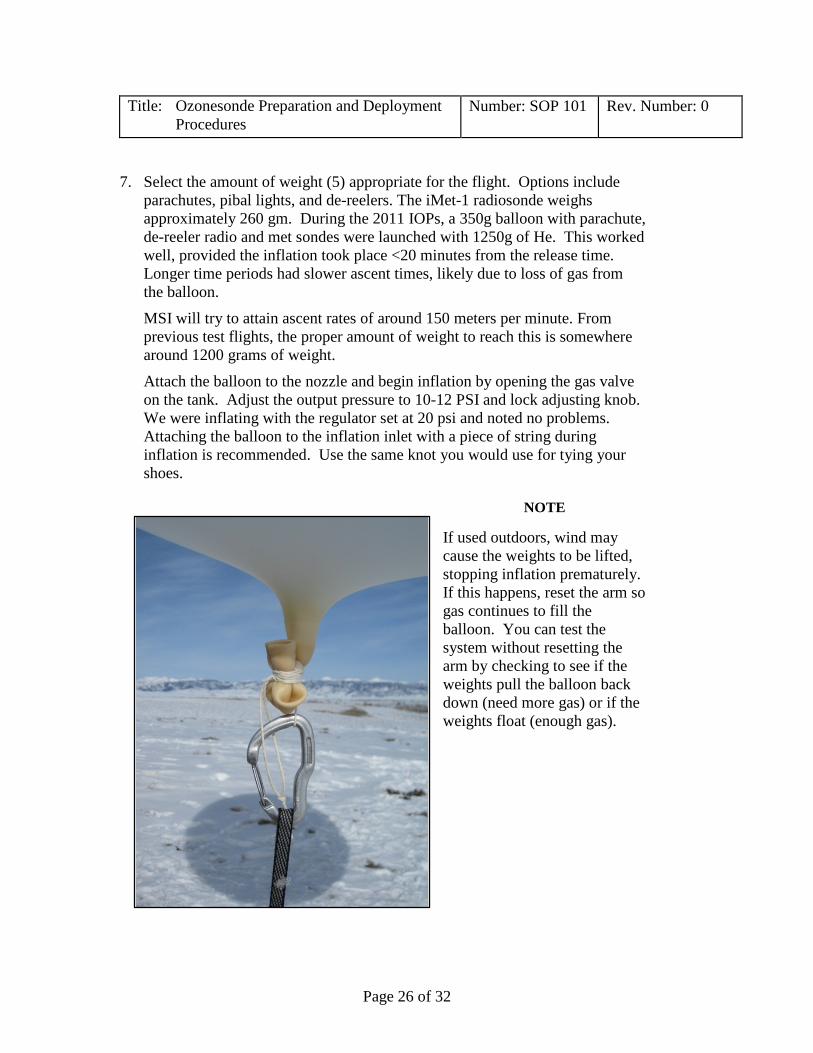
Page 26 of 32
Title: Ozonesonde Preparation and Deployment Procedures
Number: SOP 101 Rev. Number: 0
7. Select the amount of weight (5) appropriate for the flight. Options include parachutes, pibal lights, and de-reelers. The iMet-1 radiosonde weighs approximately 260 gm. During the 2011 IOPs, a 350g balloon with parachute, de-reeler radio and met sondes were launched with 1250g of He. This worked well, provided the inflation took place <20 minutes from the release time. Longer time periods had slower ascent times, likely due to loss of gas from the balloon.
MSI will try to attain ascent rates of around 150 meters per minute. From previous test flights, the proper amount of weight to reach this is somewhere around 1200 grams of weight.
Attach the balloon to the nozzle and begin inflation by opening the gas valve on the tank. Adjust the output pressure to 10-12 PSI and lock adjusting knob. We were inflating with the regulator set at 20 psi and noted no problems. Attaching the balloon to the inflation inlet with a piece of string during inflation is recommended. Use the same knot you would use for tying your shoes.
If used outdoors, wind may cause the weights to be lifted, stopping inflation prematurely. If this happens, reset the arm so gas continues to fill the balloon. You can test the system without resetting the arm by checking to see if the weights pull the balloon back down (need more gas) or if the weights float (enough gas).
NOTE

Page 27 of 32
Title: Ozonesonde Preparation and Deployment Procedures
Number: SOP 101 Rev. Number: 0
8. Once the balloon reaches the appropriate lift, the balloon will lift the weight lever arm, shutting off the gas supply to the balloon.
9. Close the gas valve on the tank. Briefly pull back the vertical valve control arm (4) to relieve the pressure in the inflation system.
10. Cut a piece of string about 4’ long, double it and tie a loop large enough to easily fit your hook/ carabiner through it.
11. Tie a series of wraps and knots to hold the neck of the balloon closed, alternating one wrap and one knot and moving down the balloon. After ¼” of wraps and knots have built up on the balloon, finish with two overhands in a row.

Page 28 of 32
Title: Ozonesonde Preparation and Deployment Procedures
Number: SOP 101 Rev. Number: 0
12. Clip the grab loop of the string to the BLP4000 (Balloon Launching Platform) and untie the bow holding the holding the balloon on the filling nozzle.
13. Finish the tie off by folding the neck of the balloon upward and tying the same series of knots you used in step 11.
14. Tie the top of the parachute to the grab loop (the shortest loop in the picture above) on the balloon.
15. Attach the de-reeler to the elastic on the bottom of the parachute hub. MSI will be using a metal ratchet type de-reeler (not pictured).
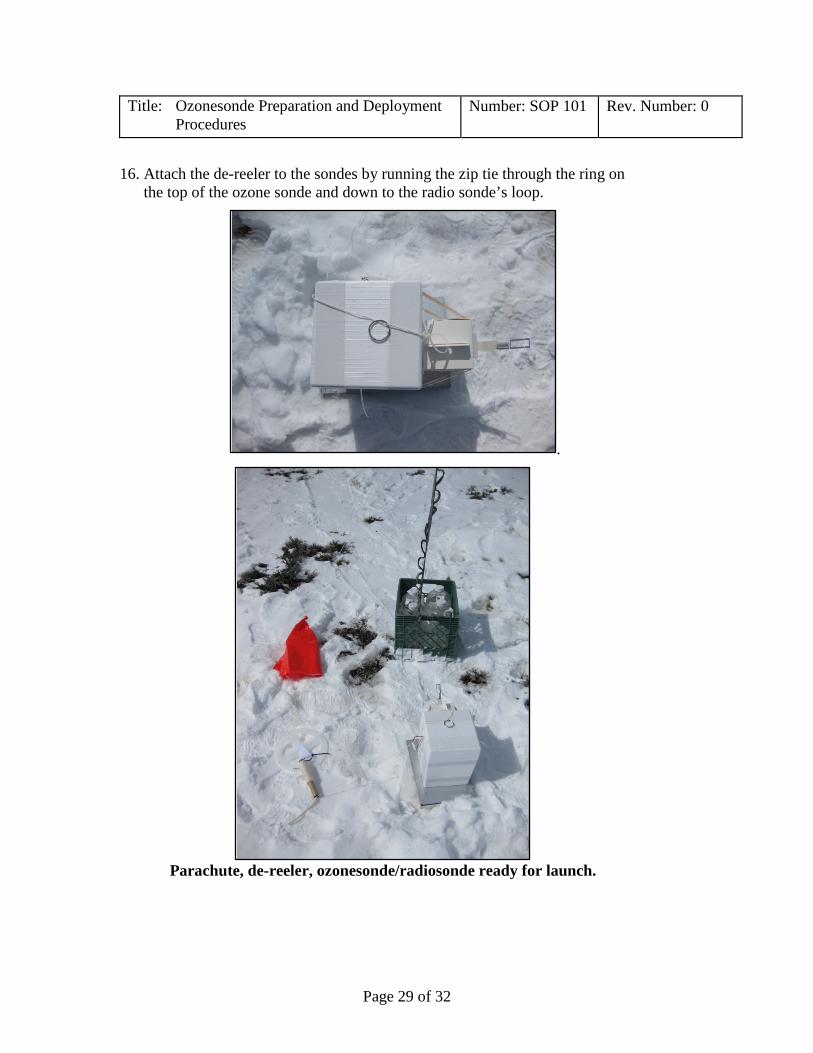
Page 29 of 32
Title: Ozonesonde Preparation and Deployment Procedures
Number: SOP 101 Rev. Number: 0
16. Attach the de-reeler to the sondes by running the zip tie through the ring on the top of the ozone sonde and down to the radio sonde’s loop.
.
Parachute, de-reeler, ozonesonde/radiosonde ready for launch.
Page 30 of 32
Title: Ozonesonde Preparation and Deployment Procedures
Number: SOP 101 Rev. Number: 0
7) DAY OF LAUNCH: LAUNCHING THE BALLOON AND COMPUTER OPERATIONS.
The 403 MHz Antenna is an omni-directional antenna. There are no restrictions for minimum launch distance between the sonde and the 403 MHz antenna. The radiosonde can be launched from directly next to the antenna as long as precautions are taken to not allow the radiosonde, string, or balloon to contact the antenna or become entangled. The radiosonde shall be held such that the body does not block the reception of GPS signals. Hold the radiosonde midway up the side of the radiosonde case.
When handling the radiosonde, take care not to damage the sensor probe. 1) On the “O3” program, ensure that the “Flight” button is highlighted
(after first detecting the ozonesonde signal, there will be about a 3-5 minute delay before the “Flight” is highlighted).
2) RELEASE THE BALLOON. Release the radiosonde as soon as the balloon tries to pull the radiosonde up.
3) Tracking the Radiosonde
Occasionally (at least every 15 minutes), double check that the receiver is accurately tuned to the radiosonde. Adjust the frequency, as necessary, such that the red line in the Scope Panel is centered between the twin peaks.
Real time graphs are available to look at in the O3 software during flight, and should be monitored as well. There are also data tables that are updated secondly and can be viewed.
Note Towards the end of the flight, the signal strength will be too weak to be displayed on the Scope Panel. However, by this point in the time, the radiosonde frequency will not change enough to impair performance. The iMet-1 radiosonde transmits data at a rate of one record per second. Moderate amounts of data loss will not prevent a successful flight and should not result in early termination unless something is clearly wrong. Data loss is more likely at the end of a flight or during periods when the sonde is directly overhead.
CAUTION

Page 31 of 32
Title: Ozonesonde Preparation and Deployment Procedures
Number: SOP 101 Rev. Number: 0
Real time graph of Ozone vs Height.
8) DAY OF LAUNCH: TERMINATING FLIGHT AND ARCHIVING FLIGHT DATA.
In the “O3” software, to terminate the flight, press “End” on the “O3” software, and “Yes”. MSI will wait at least until the sonde package has reached 500 mb (~18,000 ft), but in most cases will wait until it reaches 300 mb (~ 30,000 ft) before terminating the flight.
Once a flight has been terminated, the user cannot resume the flight. The Icom IC-PCR1500/2500 software may be closed. Push the [Power] button on the Toolbar to shut down the receiver and [Exit] to close the software. Turn off the MP and unplug the USB cable from the laptop. The InterMet O3 software outputs a series of files from each flight including separate files for GPS, Wind, PTU, Ozone, config file, and a coded Raw file. After a balloon flight is completed, the operator will connect to the network at the Boulder site and email the flight files to the MSI office for review and post processing.
Page 32 of 32
Title: Ozonesonde Preparation and Deployment Procedures
Number: SOP 101 Rev. Number: 0
9) REVIEW AND POST PROCESSING OF FLIGHT DATA. Once sonde data are received by email at MSI offices, the data are downloaded and imported into the EN-SCI ozonesonde processing software PV7. Before exporting the data, default options on the Preferences tab are changed to reduce data filtration and manipulation. These changes include the “Ozone low-pass filter” is set to 0.0 seconds and the “Show All Data” is selected. Data are then exported (as a .csv file) using the “Export All” option under the “File” dropdown menu and are ready to be plotted using RAOB. RAOB version 6.2 is used to plot ozonesonde data. To import the ozonesonde data, from the “File” dropdown menu select “Open Sounding” navigate to the .csv file created using PV7. RAOB automatically plots the temperature and wind data. Ozone data can be plotted by clicking the “Analyze” dropdown menu, a window will appear where the user selects “Ozone”. Images are then saved as a .png image to be displayed on the website by selecting “File” then “Save Image to File…”.

Appendix B Microsoft Access Database Description

The Upper Green Winter Ozone Study (UGWOS) 2013 Database
1. Introduction
This document describes the Upper Green Winter Ozone Study (UGWOS) database for 2013. Included are a review of the study measurements and descriptions of the key data reporting elements such as naming conventions, time reference and units. This document describes the overall structure of the database with a description of the data tables and file formats.
2. Overview of Measurements and Field Study Participants
The 2013 UGWOS field study included hourly measurements of surface and upper air meteorological and air quality data during the period of January through March 2013 in the upper Green River Basin region of southwestern Wyoming. Winds aloft were measured by a mini-SODAR and are reported on an hourly basis for the duration of the study. VOC data were collected at eight locations (Boulder, Juel Springs, Jonah, Jonah2, Paradise, Mesa, Warbonnet, and Big Piney) to determine spatial distribution of VOCs. The following lists the UGWOS participants and the data they submitted: Wyoming Department of Environmental Quality:
WDEQ runs an ambient air quality network throughout the state of Wyoming. Air Quality sites included in UGWOS 2013 were located in or near Sublette County in southwestern Wyoming. The stations include:
o Boulder (including 1-minute and 1-hour data collection), o Big Piney, o Daniel South, o Farson (Met Only) o Jonah, o Jonah2 (Winds and VOC only), o Juel Springs, o Hiawatha, o Mesa, o Moxa, o Murphy Ridge, o Paradise, o Pinedale, o South Pass, o Thunder Basin, o Wamsutter, o Warbonnet, and o Wyoming Range.
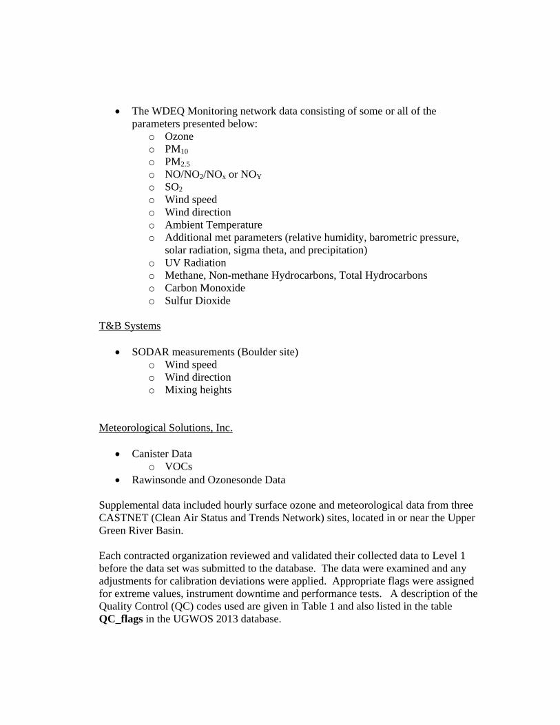
The WDEQ Monitoring network data consisting of some or all of the parameters presented below:
o Ozone o PM10 o PM2.5 o NO/NO2/NOx or NOY o SO2 o Wind speed o Wind direction o Ambient Temperature o Additional met parameters (relative humidity, barometric pressure,
solar radiation, sigma theta, and precipitation) o UV Radiation o Methane, Non-methane Hydrocarbons, Total Hydrocarbons o Carbon Monoxide o Sulfur Dioxide
T&B Systems
SODAR measurements (Boulder site)
o Wind speed o Wind direction o Mixing heights
Meteorological Solutions, Inc.
Canister Data
o VOCs Rawinsonde and Ozonesonde Data
Supplemental data included hourly surface ozone and meteorological data from three CASTNET (Clean Air Status and Trends Network) sites, located in or near the Upper Green River Basin.
Each contracted organization reviewed and validated their collected data to Level 1 before the data set was submitted to the database. The data were examined and any adjustments for calibration deviations were applied. Appropriate flags were assigned for extreme values, instrument downtime and performance tests. A description of the Quality Control (QC) codes used are given in Table 1 and also listed in the table QC_flags in the UGWOS 2013 database.

Table 1 - Data Flags QC Description V Valid Data M Missing Data I Invalid Data S Suspect Data - Data appears to be a data spike or outside normal data
range U Data which has not been validated - User is responsible for validation. N Instrument Noise detected in sub hourly data used to create hourly
average B Below Detection Limit AA Sample Pressure out of Limits AB Technician Unavailable AC Construction/Repairs in Area AD Shelter Storm Damage AE Shelter Temperature Outside Limits AF Scheduled but not Collected AG Sample Time out of Limits AH Sample Flow Rate out of Limits AI Insufficient Data (cannot calculate) AJ Filter Damage AK Filter Leak AL Voided by Operator AM Miscellaneous Void AN Machine Malfunction AO Bad Weather AP Vandalism AQ Collection Error AR Lab Error AS Poor Quality Assurance Results AT Calibration AU Monitoring Waived AV Power Failure AW Wildlife Damage AX Precision Check AY Q C Control Points (zero/span) AZ Q C Audit BA Maintenance/Routine Repairs BB Unable to Reach Site BC Multi-point Calibration BD Auto Calibration BE Building/Site Repair BF Precision/Zero/Span

Table 1 Continued - Data Flags QC Description BG Missing ozone data not likely to exceed level of standard BH Interference/co-elution/misidentification BI Lost or damaged in transit BJ Operator Error BK Site computer/data logger down BL QA Audit BM Accuracy check BN Sample Value Exceeds Media Limit B Below Detection Limit
3. UGWOS Database Design
Meteorological Solutions Inc. assimilated the submitted data into an Access 2010 database called UGWOS_2013_Database_Version?.?.accdb (where ?.? indicates version number). The database consists of both information and data files. It has a simple straightforward design. The Sites table contains all of the site information (site name, site identification code used in all of the data tables, site location including latitude, longitude, elevation, and a tabular list of what parameters were measured at each site and the organization responsible). The Parameters table lists parameter codes used in the data tables. The table named Updates lists all information pertaining to modifications and versions of the data as well as dates of said modifications. The name of the database includes a version number to help users identify the most current version of the database.
All data files submitted were examined carefully to verify unique site codes for all sites, instruments, and parameters so that no orphan or duplicate records exist in any of the tables. The valid data were examined for completeness and reasonableness of data ranges. All invalid or missing data were verified to have the adverse AQS Null code values or the value –9999. All of the date and times are in begin hour (0-23) Mountain Standard Time. The data were organized and grouped together by platform, averaging period and data type. The Hourly Air Quality table includes hourly average data of criteria pollutants (ozone, oxides of nitrogen, particulate matter) measured at each of the sites. Other pollutants such as methane, non-methane hydrocarbons and total hydrocarbons are also included in the Hourly Air Quality Table. One minute air quality data were collected at the Boulder site. These data are presented in the 1-minute Air Quality data table. Boulder data went through quality assurance with valid data marked with a “V” in the QC flag field.

Data included in the Hourly Meteorology table represent hourly averages of meteorological data parameters such as wind speed, wind direction, standard deviation of the wind direction, and temperature. Select sites have additional meteorological parameters such as relative humidity, solar radiation, barometric pressure, dew point temperature, precipitation, and UV radiation. One minute meteorological data were collected at the Boulder and Mobile trailer sites. These data are presented in the 1-minute Meteorology data table. Boulder data went through quality assurance. The Mobile Trailer did not get validated and the data has a QC flag of “U” as specified in Table 1 as data which has not been validated.
The 8-Hour Ozone table includes the leading 8-hour average of ozone for each of the sites.
Upper air data including the data from the SODAR is provided in the Sodar and the Mixing Height data tables. Radiosonde and Ozonesonde data are presented in Sonde Data (Met Only) and Sonde Data (Ozone) tables. Surface VOC data collected during IOPs at the Boulder, Juel Springs, Jonah, and Big Piney sites are presented in the VOC table. A summary of the canister data collected at the VOC sites are available in VOC Summary table. The data tables all have a flat format with the identifying information in the starting columns. The most common parameters are listed first. An empty data column and quality control flag indicates no measurements obtained at the site for that parameter. Additional documentation that includes a complete description of the data column, units, etc. is provided by Access 2010 in the information bar at the bottom of the Access window screen when the user is accessing the column. All data tables include a Record Number column at the end of the table, this column is intended to keep data sorted in chronological order by site to match the Sites table. With this option, a user can sort the table any way he or she chooses and have the capability of sorting the table into its original format. The data have the following general unit configurations:
Parts per billion for O3, NO, NO2, NOX, NOY, and SO2 Micrograms per cubic meter for PM10 and PM2.5 Parts per million for methane, non-methane hydrocarbons, and total
hydrocarbons Micrograms per cubic meter, parts per billion by volume, and parts per
billion by Carbon for VOC data, Meters per second for wind speed Degrees Celsius for ambient temperature and dew point temperature Watts per meter squared for solar radiation and ultra violet radiation Percent for relative humidity

The 2013 UGWOS database contains data queries for quick data sorting based on a users needs. There are four queries for users to gain access to data (Days and Hours of Data, Individual Site Data, Sort 1-hour Ozone Data, and Sort 8-hour Ozone Data). Once a user opens the query he or she will be asked some pertinent questions for the query. After the questions have been answered, the query will sort the data as designed. A more complete description of each query is below:
Days and Hours of Data- this query simply asks for the date and hours of data the user is looking for. The user is first asked to give a “Starting Date” and an “Ending Date”; these should fall within the UGWOS period of January 15, 2013 and March 31, 2013. Next the user will be asked for an hour beginning and an hour ending, the data are in hour beginning format (0-23). Data not between the specified beginning and ending hours will be removed for all days between the starting and ending dates. Individual Site Data- The database has several tables with data sorted by air quality, meteorological, site information parameters, etc. This query takes all of the air quality and meteorological data from one station and places it into an individual table. The user will be asked for the five character alpha numeric “Station Code” found in the Sites table. Once a matching station code is entered the meteorological and air quality data will be output into one table. Sort 1-hour Ozone Data- the purpose of this query and the Sort 8-hour Ozone Data query are to sort any data above a user specified threshold. The user will be asked to provide a level of which no data records with an ozone level below that threshold will be displayed. Common parameters are displayed in each data record.
All additional field names are described in the Parameters table. Users wishing to be notified of updates to the database can send their e-mail address to the UGWOS Database Manager, Scott Adamson, at [email protected].
4. Summary
This document describes the 2013 UGWOS database. Feedback from study participants concerning this document and the database is requested and any suggestions for improvement are highly encouraged and appreciated.


