
MS Excel Advanced Level Ramzan Rajani
MS Excel Advanced Level
Trainer : Ramzan Rajani
MS Excel Advanced Level Ramzan Rajani
Contents
Conditional Formatting ....................................................................................................................................... 1
Remove Duplicates .............................................................................................................................................. 4
Sorting ................................................................................................................................................................. 5
Filtering ................................................................................................................................................................ 6
Charts →Column ................................................................................................................................................. 7
Charts → Line .................................................................................................................................................... 10
Charts → Bar ..................................................................................................................................................... 10
Charts → Pie ...................................................................................................................................................... 11
Charts → Target Line ........................................................................................................................................ 12
Charts →Two Axis Chart (Secondary Axis) ........................................................................................................ 13
Pivot table .......................................................................................................................................................... 14
Example uses of Pivot Tables ................................................................................................................. 14
Excel Pivot Table Tutorial: How to create your first pivot table ........................................................ 15
Some useful tips on Excel Pivot Tables .................................................................................................. 17
Header & Footer ................................................................................................................................................ 18
Text to Column .................................................................................................................................................. 19
Data Validation – Creating drop down list ........................................................................................................ 21
Sub total ............................................................................................................................................................ 22
Importing Text & Access File ............................................................................................................................. 23
Inserting comments ........................................................................................................................................... 27
Protect Sheet ..................................................................................................................................................... 28
Protect Workbook ............................................................................................................................................. 29
Password while opening the file ....................................................................................................................... 30
Freeze / Unfreeze .............................................................................................................................................. 31
Sharing file ......................................................................................................................................................... 32
View multiple Excel workbooks ......................................................................................................................... 33
Recording & Running Macros (Non Programming) ........................................................................................... 34
Sparklines (2010 & above version only) ............................................................................................................ 36
Hyperlinking ....................................................................................................................................................... 37
Inserting dynamic table ..................................................................................................................................... 38
Paste Special ...................................................................................................................................................... 39

MS Excel Advanced Level Ramzan Rajani
1 | P a g e
Conditional Formatting
By applying conditional formatting to your data, you can quickly identify variances in a range of values with a quick glance
• After selecting the data select one of the options to apply it to the selected cells.
A cascading menu will appear.
Data Bars: This is an interesting option that formats the selected cells with colored bars. The length of the data bar represents the value in the cell. The longer the bar, the higher the value.

MS Excel Advanced Level Ramzan Rajani
2 | P a g e
Icon sets:
Highlight duplicate records
MS Excel Advanced Level Ramzan Rajani
3 | P a g e
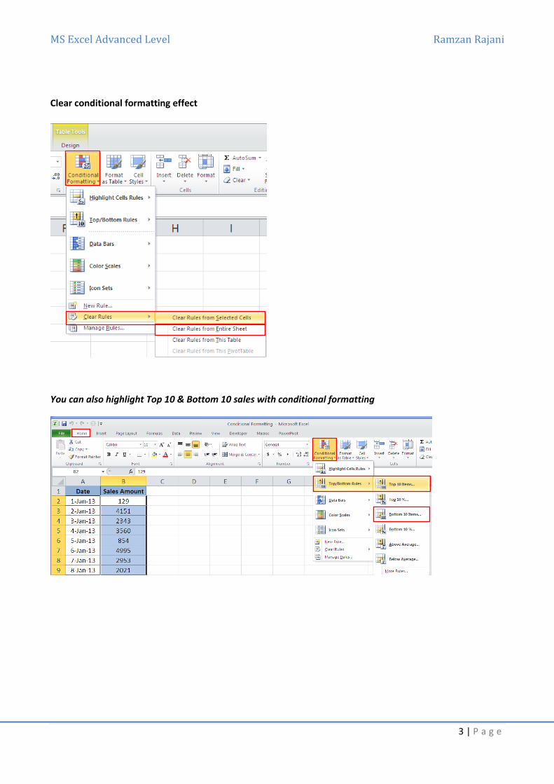
Clear conditional formatting effect
You can also highlight Top 10 & Bottom 10 sales with conditional formatting

MS Excel Advanced Level Ramzan Rajani
4 | P a g e
Remove Duplicates
This example teaches you how to remove duplicates in Excel
1. Click any single cell inside the data set.
2. On the Data tab, click Remove Duplicates.
The following dialog box appears.
3. Leave all checkboxes checked and click OK.
Result. Excel removes all identical rows (blue) except for the first identical row found (yellow).

MS Excel Advanced Level Ramzan Rajani
5 | P a g e
Sorting
When you sort information in a worksheet, you can see data the way you want and find values quickly. You can sort a range or table of data on one or more columns of data; for example, you can sort employees first by department and then by last name.
Sorting lists is a common spreadsheet task that allows you to easily reorder your data. The most common
type of sorting is alphabetical ordering, which you can do in ascending or descending order.
To Sort in Alphabetical Order:
• Select a cell in the column you want to sort (In this example, we choose a cell in column A).
• Click the Sort & Filter command in the Editing group on the Home tab.
• Select Sort A to Z. Now the information in the Category column is organized in alphabetical
order
OR
Remember all of the information and data is still here. It's just in a different order.
Shortcut of sorting: Alt D S

MS Excel Advanced Level Ramzan Rajani
6 | P a g e
Filtering
By filtering information in a worksheet, you can find values quickly. You can filter on one or more columns of data. With filtering, you can control not only what you want to see, but what you want to exclude. You can filter based on choices you make from a list, or you can create specific filters to focus on exactly the data that you want to see.
This allows you to focus on specific spreadsheet entries.
To remove all filters, click the Filter command once again or press the below shortcut
Shortcut of filtering: Ctrl Shift L

MS Excel Advanced Level Ramzan Rajani
7 | P a g e
Charts →Column
A chart is a tool you can use in Excel to communicate your data graphically. Charts allow your audience to more easily see the meaning behind the numbers in the spreadsheet, and make showing comparisons and trends a lot easier.
To Create a Chart:
• Select the cells that you want to chart, including the column titles and the row labels.
• Click the Insert tab.
• Hover over each Chart option in the Charts group to learn more about it.
• Select one of the Chart options. In this example, we use the Columns command.
• Select a type of chart from the list that appears. For this example, we use a 2-D Clustered
Column. The chart appears in the worksheet.
Identifying the Parts of a Chart

MS Excel Advanced Level Ramzan Rajani
8 | P a g e
To Change the Chart Type:
• Select the Design tab.
• Click the Change Chart Type command. A dialog box appears.
• Select another chart type.
• Click OK.
To Change Chart Layout:
• Select the Design tab.
• Locate the Chart Layouts group.
• Click the Morearrow to view all your layout options.
• Left-click a layout to select it.

MS Excel Advanced Level Ramzan Rajani
9 | P a g e
To Change Chart Style:
• Select the Design tab.
• Locate the Chart Style group.
• Click the Morearrow to view all your style options.
• Left-click a style to select it.
To Move the Chart to a Different Worksheet:
• Select the Design tab.
• Click the Move Chart command. A dialog box appears. The current location of the chart is
selected.
• Select the desired location for the chart (i.e., choose an existing worksheet, or select New Sheet
and name it).

MS Excel Advanced Level Ramzan Rajani
10 | P a g e
Charts → Line
Data that is arranged in columns or rows on a worksheet can be plotted in a line chart. Line charts can display continuous data over time, set against a common scale, and are therefore ideal for showing trends in data at equal intervals.
Charts → Bar

MS Excel Advanced Level Ramzan Rajani
11 | P a g e
Charts → Pie
Useful when you want to show the data in percentage %

MS Excel Advanced Level Ramzan Rajani
12 | P a g e
Charts → Target Line
To show Actuals V/s Target

MS Excel Advanced Level Ramzan Rajani
13 | P a g e
Charts →Two Axis Chart (Secondary Axis)
To show larger number on one Axis & smaller numbers on secondary axis
Steps :
1) After creating a 2D column chart
2) Select the Experience axis
3) Go to Layout tab of chart & click on Format Selection
4) Select Secondary Axis
5) Change Experience bar into Line chart

MS Excel Advanced Level Ramzan Rajani
14 | P a g e
Pivot table
PivotTables are one of the most powerful Microsoft Excel tools available. It is used to summarize complex & huge database into summary form.
Pivot tables
Excel pivot tables are very useful and powerful feature of MS Excel. They can be used to
summarize, analyze, explore and present your data.
In plain English, it means, you can take the sales data with columns like salesman, region and
product-wise revenues and use pivot tables to quickly find out how products are performing in each
region.
In this tutorial, we will learn what is a pivot table and how to make a pivot table using excel.
Example uses of Pivot Tables
As I said before pivot tables are very powerful and useful. There are numerous uses of pivot tables
that we can talk about them until Christmas.
Here are some example uses of pivot tables:
• Summarizing data like finding the average sales for each region for each product from a
product sales data table.
• Listing unique values in any column of a table
• Creating a pivot report with sub-totals and custom formats
• Making a dynamic pivot chart
• Filtering, sorting, drilling-down data in the reports without writing one formula or macro.
• Transposing data – i.e. moving rows to columns or columns to rows. [learn more]
• Linking data sources outside excel and be able to make pivot reports out of such data.

MS Excel Advanced Level Ramzan Rajani
15 | P a g e
Excel Pivot Table Tutorial: How to create your first pivot table
Let us make your first pivot table. We will use example data in the following format. Open the file
with the name → Excel-Pivot-tables-tutorial
Step 1: Select the data
Select the data range from which you want to make the pivot table.
Step 2: Go to Insert ribbon and click on new Pivot table option
To insert a new pivot table in to your spreadsheet, go to Insert ribbon and click
pivot table icon and select pivot table option.
Step 3: Select the target cell where you want to place the pivot table. For
starters, select New worksheet.
Excel will display a pivot table wizard where you can specify the pivot table
target location etc. Select “New worksheet” option and your pivot table will be placed in newly
created worksheet.
Step 4: Make your first pivot report
The pivot report UI is very intuitive and sandbox like. To make powerful analysis, all you have to do
is drag and drop fields in to the pivot table grid area. In excel 2007, you can also control this by
using the “Pivot table panel”.
The pivot report is divided in to header and body sections. You can drag and drop the fields you want
in each area. The body itself contains three parts. Rows, Columns and Cells. You can use any fields
in these areas too.
For the above sample data, I have set this criteria:

MS Excel Advanced Level Ramzan Rajani
16 | P a g e
And the outcome is this pivot report.
It might be a bit difficult to understand how this works. But believe me, if you have seen any reports
or worked with any other reporting systems, then the idea of pivot tables, pivot reports and pivot
charts becomes quite simple to you.

MS Excel Advanced Level Ramzan Rajani
17 | P a g e
You can use the excel pivot table features to make a more complicated pivot report like this in no
time.
Some useful tips on Excel Pivot Tables
• You can apply any formatting to the pivot tables. MS Excel has some very good pivot table
formats (and they are better in Excel 2007 and 2010).
• You can easily change the pivot table summary formulas. Right click on pivot table and
select “summarize data by” option.
• You can also apply conditional formatting on pivot tables although you may want to be a bit
careful as pivot tables scale in size depending on the data.
• Whenever the original data from which pivot tables are constructed, just right click on the
pivot table and select “Refresh Data” option.
• If you want to drill down on a particular summary value, just double click on it. Excel will
create a new sheet with the data corresponding to that pivot report value. (This is extremely
useful)
• Making a pivot chart from a pivot table is very simple. Just click on the pivot chart icon from
tool bar or Options ribbon area and follow the wizard.

MS Excel Advanced Level Ramzan Rajani
18 | P a g e
Header & Footer
Headers and footers are lines of text that print at the top (header) and bottom (footer) of each page in the spreadsheet. They contain descriptive text such as titles, dates, and/or page numbers.
(1)
(2)
(3)
MS Excel Advanced Level Ramzan Rajani
19 | P a g e
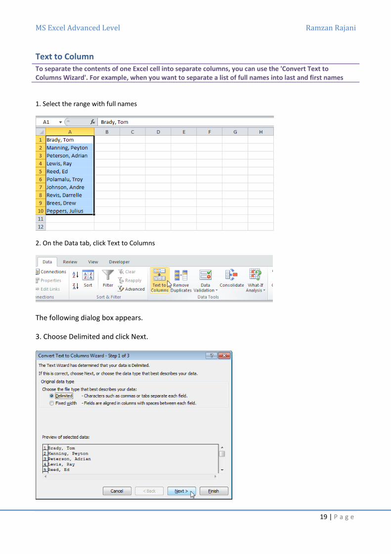
Text to Column
To separate the contents of one Excel cell into separate columns, you can use the 'Convert Text to Columns Wizard'. For example, when you want to separate a list of full names into last and first names
1. Select the range with full names
2. On the Data tab, click Text to Columns
The following dialog box appears.
3. Choose Delimited and click Next.

MS Excel Advanced Level Ramzan Rajani
20 | P a g e
4. Clear all the checkboxes under Delimiters except for the Comma and Space checkbox.
5. Click Finish
Note: This example has commas and spaces as delimiters. You may have other delimiters in your data. Experiment by checking and unchecking the different checkboxes. You get a live preview of how your data will be separated.
Result:
Practice file name: text-to-columns

MS Excel Advanced Level Ramzan Rajani
21 | P a g e
Data Validation – Creating drop down list
Drop-down lists in Excel are helpful if you want to be sure that users select an item from a list, instead of typing their own values.
1. On the first sheet, select cell B1.
3. On the Data tab, click Data Validation
4. Type the items directly into the textbox.

MS Excel Advanced Level Ramzan Rajani
22 | P a g e
Sub total
Total several rows of related data together by automatically inserting subtotals and totals for the selected cells.
Steps:
1) Sort the data on the column on which you need to do subtotals
2) Go to data Ribbon and click on Subtotal (see below screen shot)
3) At each change in → Select -- Region
4) Use function→ Sum
5) Add subtotal to→Select -- Sales column

MS Excel Advanced Level Ramzan Rajani
23 | P a g e
Importing Text & Access File
This describes how to import or export text files. Text files can be comma separated (.csv) or tab separated (.txt)
To import text files, execute the following steps.
1. On the File tab, click Open. (Excel 2010) in Excel 2007 click on Top Left office logo
2. Select Text Files from the drop-down list.
3a. To import a .csv file, select the .csv file and click Open. That's all.
3b. To import a .txt file, select the .txt file and click Open. Excel launches the Text Import Wizard.
4. Choose Delimited and click Next.

MS Excel Advanced Level Ramzan Rajani
24 | P a g e
5. Clear all the checkboxes under Delimiters except for the Tab checkbox and click Next.
6. Click Finish.

MS Excel Advanced Level Ramzan Rajani
25 | P a g e
Result:
Export
To export text files, execute the following steps.
1. Open an Excel file.
2. On the File tab, click Save As.
3. Select Text (Tab delimited) or CSV (Comma delimited) from the drop-down list.

MS Excel Advanced Level Ramzan Rajani
26 | P a g e
4. Click Save. Result. A .csv file (comma separated) or a .txt file (tab separated).
Practice file: data-set

MS Excel Advanced Level Ramzan Rajani
27 | P a g e
Inserting comments
You can insert a comment to give feedback about the content of a cell.
Insert Comment
To insert a comment, execute the following steps.
1. Select a cell.
2. Right click and then click Insert Comment.
Practice File: comments

MS Excel Advanced Level Ramzan Rajani
28 | P a g e
Protect Sheet
When you share a file with other users, you may want to protect a worksheet to help prevent it from being changed.
1. Right click on the worksheet tab of the worksheet you want to protect. 2. Click Protect Sheet...
3. Enter a password. 4. Check the actions you allow the users of your worksheet to perform. 5. Click OK.
6. Confirm the password and click OK.
Your worksheet is protected now. The password for the downloadable Excel file is easy Note: to unprotect a worksheet, right click on the worksheet tab again and click Unprotect Sheet..
Practice file: protect-sheet

MS Excel Advanced Level Ramzan Rajani
29 | P a g e
Protect Workbook
Protects your sheet from Deletion.
MS Excel Advanced Level Ramzan Rajani
30 | P a g e
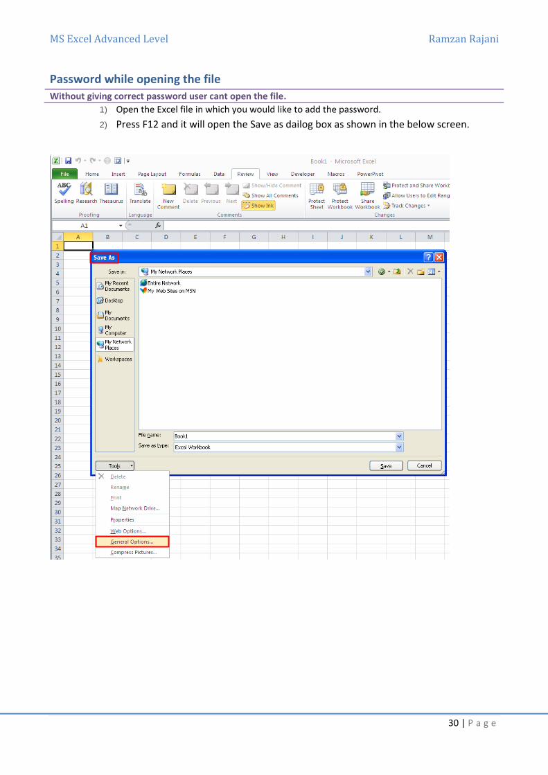
Password while opening the file
Without giving correct password user cant open the file.
1) Open the Excel file in which you would like to add the password.
2) Press F12 and it will open the Save as dailog box as shown in the below screen.

MS Excel Advanced Level Ramzan Rajani
31 | P a g e
Freeze / Unfreeze
If you have a large table of data in Excel, it can be useful to freeze rows or columns. This way you can keep rows or columns visible while scrolling through the rest of the worksheet
To freeze the top row, execute the following steps. 1. On the View tab, click Freeze Panes, Freeze Top Row.
2. Scroll down to the rest of the worksheet.
Result. Excel automatically adds a black horizontal line to indicate that the top row is frozen.
Unfreeze Panes
Practice file: freeze-panes

MS Excel Advanced Level Ramzan Rajani
32 | P a g e
Sharing file
If you share a workbook, you can work with other people on the same workbook at the same time. The workbook should be saved to a network location where other people can open it. You can keep track of the changes other people make and accept or reject those changes.
To share a workbook, execute the following steps. 1. Open a workbook. 2. On the Review tab, in the Changes group, click Share Workbook.
Practice file: share-workbooks
MS Excel Advanced Level Ramzan Rajani
33 | P a g e
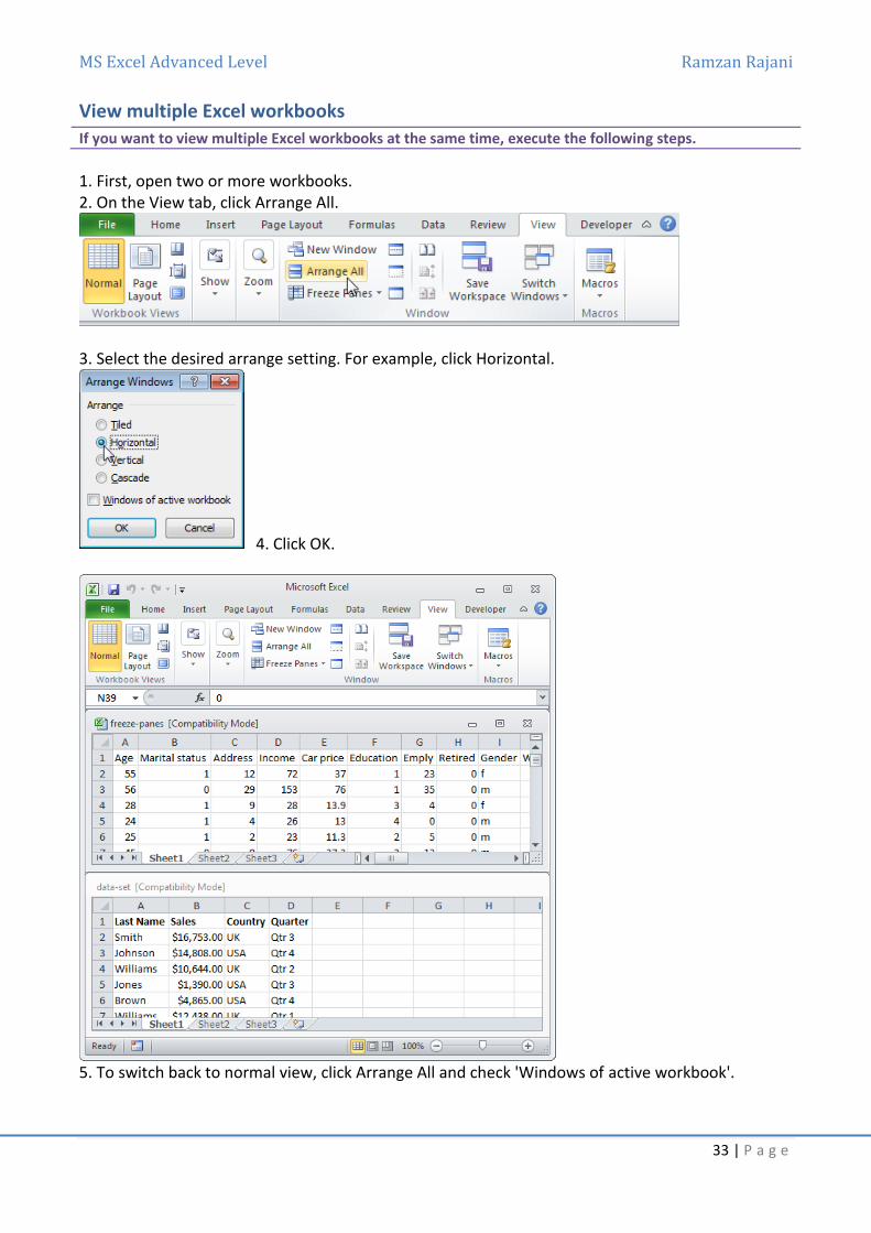
View multiple Excel workbooks
If you want to view multiple Excel workbooks at the same time, execute the following steps.
1. First, open two or more workbooks. 2. On the View tab, click Arrange All.
3. Select the desired arrange setting. For example, click Horizontal.
4. Click OK.
5. To switch back to normal view, click Arrange All and check 'Windows of active workbook'.
MS Excel Advanced Level Ramzan Rajani
34 | P a g e
Recording & Running Macros (Non Programming)
A macro is a customized collection of commands which can be executed on demand to carry out aparticular action in Excel. Since macros can include many different commands which aresubsequently performed automatically by the computer, they are very useful for performingrepetitive or complex tasks and for saving time.
First Plan Your Macro Before recording a macro plan exactly what you want it to do and practice carrying out theprocedure manually. You might find it useful to write down the steps involved so that you don'tmake any mistakes when making the recording. Think about how you will use the macro and try togeneralise the commands so that your macro will work in as many different situations as possible.
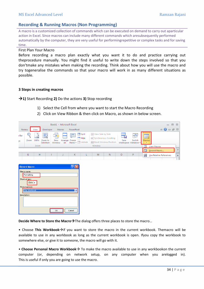
3 Steps in creating macros
→1) Start Recording 2) Do the actions 3) Stop recording
1) Select the Cell from where you want to start the Macro Recording
2) Click on View Ribbon & then click on Macro, as shown in below screen.
Decide Where to Store the Macro→The dialog offers three places to store the macro…
• Choose This Workbook→if you want to store the macro in the current workbook. Themacro will be
available to use in any workbook as long as the current workbook is open. Ifyou copy the workbook to
somewhere else, or give it to someone, the macro will go with it.
• Choose Personal Macro Workbook→ To make the macro available to use in any workbookon the current
computer (or, depending on network setup, on any computer when you arelogged in).
This is useful if only you are going to use the macro.

MS Excel Advanced Level Ramzan Rajani
35 | P a g e
• Choose New Workbook→if you don't want to use either of the other options, perhaps
because you want to create an Excel Add-In to distribute the macro to other users.

MS Excel Advanced Level Ramzan Rajani
36 | P a g e
Sparklines (2010 & above version only)
Excel 2010 makes it possible to insert sparklines. Sparklines are graphs that fit in one cell and give you information about the data.
To insert sparklines, execute the following steps. 1. Select the cells where you want the sparklines to appear. In this example, we select the range
G2:G4.
2. On the Insert tab, in the Sparklines group, click Line.
3. Click in the Data Range box and select the range A2:F4.
Practice file:sparklines
4. Click OK.
MS Excel Advanced Level Ramzan Rajani
37 | P a g e
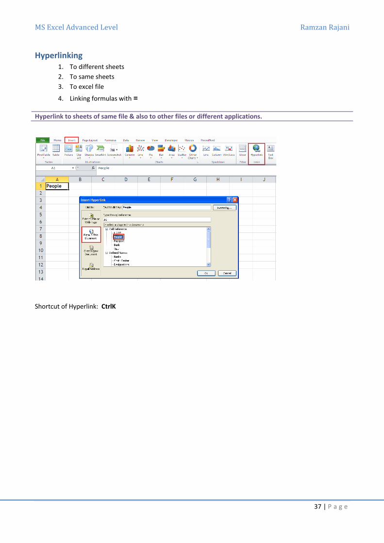
Hyperlinking 1. To different sheets
2. To same sheets
3. To excel file
4. Linking formulas with =
Hyperlink to sheets of same file & also to other files or different applications.
Shortcut of Hyperlink: CtrlK

MS Excel Advanced Level Ramzan Rajani
38 | P a g e
Inserting dynamic table
When you create a table (previously known as list) in a Microsoft Excel worksheet you can manage and analyze the data in that table independently. For example, you can filter table columns, add a row for totals, apply table formatting, automatic freeze & dynamic range for table & vlookup formula also you can publish a table to a server that is running Windows SharePoint Services 3.0 or Microsoft SharePoint Foundation 2010.
If you no longer want to work with your data in a table, you can convert the table to a regular range of data
while keeping any table style formatting that you applied. When you no longer need a table and the data
that it contains, you can delete it.
Create a table You can use one of two ways to create a table. You can either insert a table in the default table style or you can format your data as a table in a style that you choose. INSERT A TABLE USING THE DEFAULT TABLE STYLE
1. On a worksheet, select the range of cells that you want to include in the table. The cells can be
empty or can contain data.
2. On the Insert tab, in the Tables group, click Table.
Keyboard shortcut: CTRL+L OR CTRL+T
3. If the selected range contains data that you want to display as table headers,
select the My table has header

MS Excel Advanced Level Ramzan Rajani
39 | P a g e
Paste Special
Copy specific cell contents or attributes in a worksheet.
You can copy and paste specific cell contents (such as formulas, formats, or comments) from the Clipboard in
a worksheet by using the Paste Special command.
Steps:
3) On a worksheet, select the cells that contain the data or attributes that you want to copy.
4) On the Home tab, in the Clipboard group, click Copy . Or Press CTRL C
5) Select the other sheet or any other cell where you want to paste
6) Press CTRL ALT V to paste
Click this option To
All Paste all cell contents and formatting.
Formulas Paste only the formulas as entered in the formula bar.
Values Paste only the values as displayed in the cells.
Formats Paste only cell formatting.
Comments Paste only comments attached to the cell.
Column widths Paste the width of one column or range of columns to another column or range of
columns.
Values and number formats Paste only values and number formatting options from the selected cells.
Transpose To convert Horizontal data in Vertical


