
MULTI-AGENT SYSTEM GRID OPTIMIZATION
Monjur Mourshed
Piccadilly circus by LS Lowry
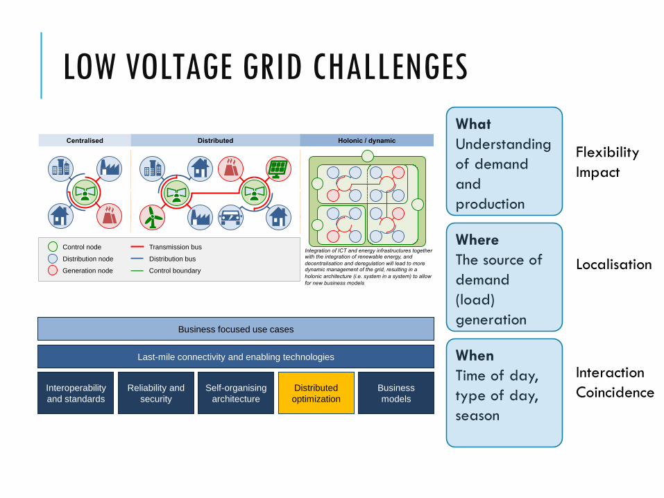
LOW VOLTAGE GRID CHALLENGES
Centralised Distributed Holonic / dynamic
Generation node
Distribution node
Control node
Control boundary
Distribution bus
Transmission bus Integration of ICT and energy infrastructures together with the integration of renewable energy, and
decentralisation and deregulation will lead to more dynamic management of the grid, resulting in a
holonic architecture (i.e. system in a system) to allow
for new business models
Past Future
What
Understanding
of demand
and
production
Where
The source of
demand
(load)
generation
When
Time of day,
type of day,
season
Interoperability
and standards
Reliability and
security
Self-organising
architecture
Distributed
optimization
Business
models
Last-mile connectivity and enabling technologies
Business focused use cases
Flexibility
Impact
Interaction
Coincidence
Localisation
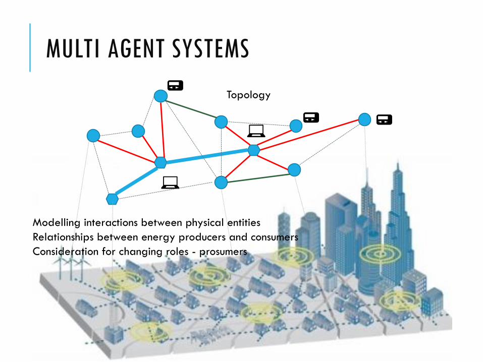
MULTI AGENT SYSTEMS
💻📟
💻
📟
📟
Modelling interactions between physical entities
Relationships between energy producers and consumers
Consideration for changing roles - prosumers
Topology

MAS HOLONIC PLATFORM FOR OPTIMIZATION AND MANAGEMENT
DSO
= Local DispatcherDistrict Manager
Home
Home
Storage
Smart
Appliance
District
DER
District
StorageHome Home
Smart
Appliance
Home
DER
Contracted energy flow
consumption
production
management
+ Flexibility Pool Manager
CEA

MAS2TERING AGENT HIERARCHY
Control and optimization strategies are based on:
• Actor roles and goals
• Business functions
• Statutory requirementsCEA
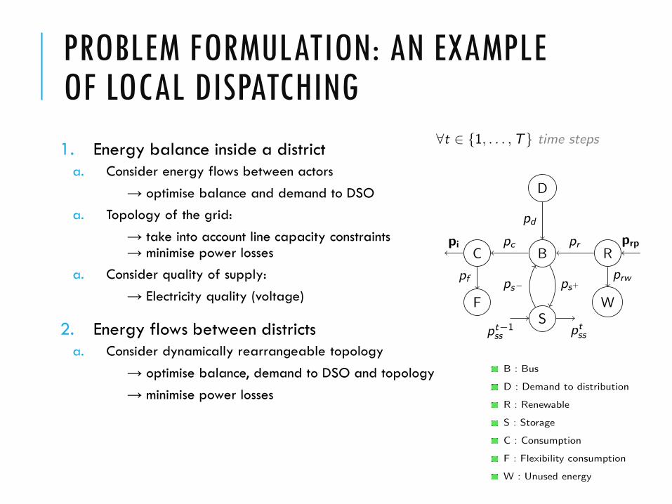
PROBLEM FORMULATION: AN EXAMPLE OF LOCAL DISPATCHING
1. Energy balance inside a district
a. Consider energy flows between actors
→ optimise balance and demand to DSO
a. Topology of the grid:
→ take into account line capacity constraints→ minimise power losses
a. Consider quality of supply:
→ Electricity quality (voltage)
2. Energy flows between districts
a. Consider dynamically rearrangeable topology
→ optimise balance, demand to DSO and topology
→ minimise power losses
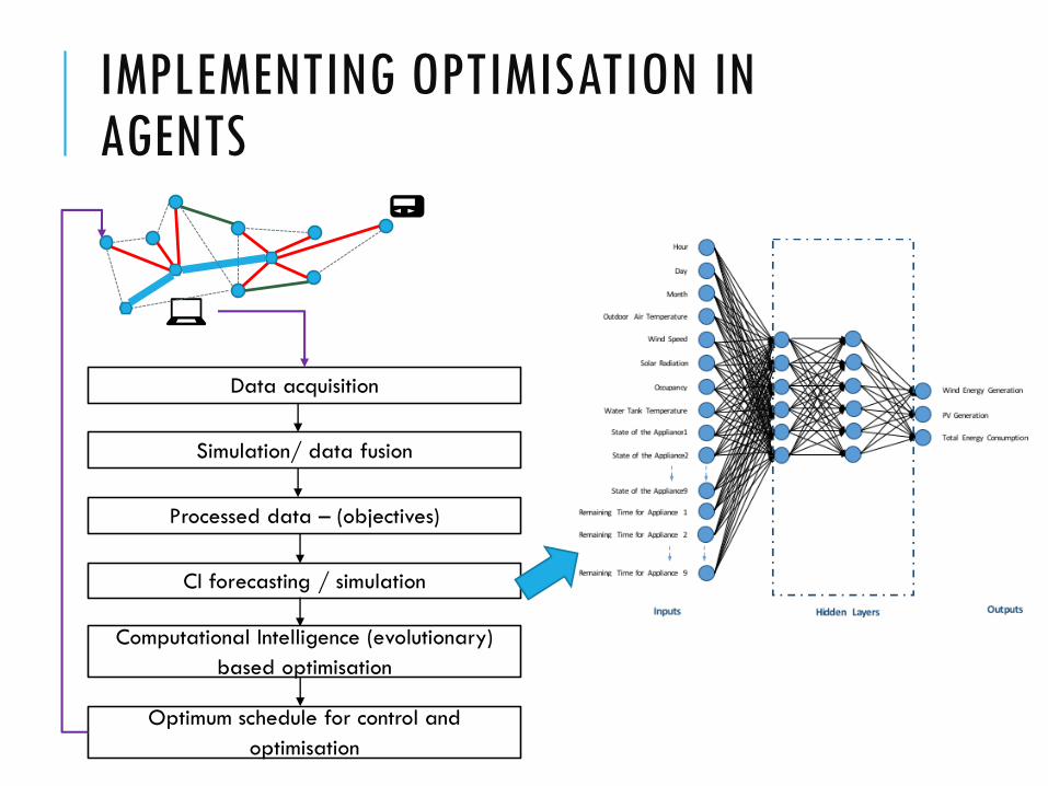
IMPLEMENTING OPTIMISATION IN AGENTS
💻
📟
Data acquisition
Simulation/ data fusion
Processed data – (objectives)
CI forecasting / simulation
Computational Intelligence (evolutionary)
based optimisation
Optimum schedule for control and
optimisation

SITUATION ASSESSMENT AND FORECASTING: DISAGGREGATED
Temp (t), Hum (RH)
Weather DER generation Appliances Seasonal
Solar irradiation (I)
Wind (v, θ)
Cloud cover (C)
Wind (turbine char.)
PV (type, size, loc.)
Deferrable
White goods
Storage
EV
Behaviour
Disaggregated forecasting
Effect is accounted
for by weather
parameters if
machine learning
or CI is used for
forecasting

FORECASTING AND OPTIMISATION AT HOME WITH PV
Implemented
In a pilot house
February – March
2015
Optimised ANN-
Priority Based
Intelligent Appliance
Scheduler
…………………………………………………
DB
Device Initial
Configurations
Weather Data
Web-Services
D1 D2 DN
Device Controller
Challenges
• Disaggregated (device) forecasting very
sensitive to occupant behaviour
• Weather data (spatial and temporal) has
significant effect on demand and
production
• Solar and wind vary significantly
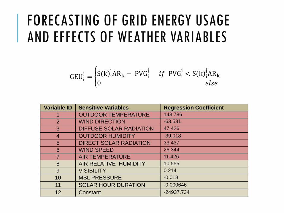
FORECASTING OF GRID ENERGY USAGE AND EFFECTS OF WEATHER VARIABLES
GEUij= S(k i
jARk − PVGi
j𝑖𝑓 PVGi
j< S(k i
jARk
0 𝑒𝑙𝑠𝑒
Variable ID Sensitive Variables Regression Coefficient
1 OUTDOOR TEMPERATURE 148.786
2 WIND DIRECTION -63.531
3 DIFFUSE SOLAR RADIATION 47.426
4 OUTDOOR HUMIDITY -39.018
5 DIRECT SOLAR RADIATION 33.437
6 WIND SPEED 26.344
7 AIR TEMPERATURE 11.426
8 AIR RELATIVE HUMIDITY 10.555
9 VISIBILITY 0.214
10 MSL PRESSURE -0.018
11 SOLAR HOUR DURATION -0.000646
12 Constant -24937.734
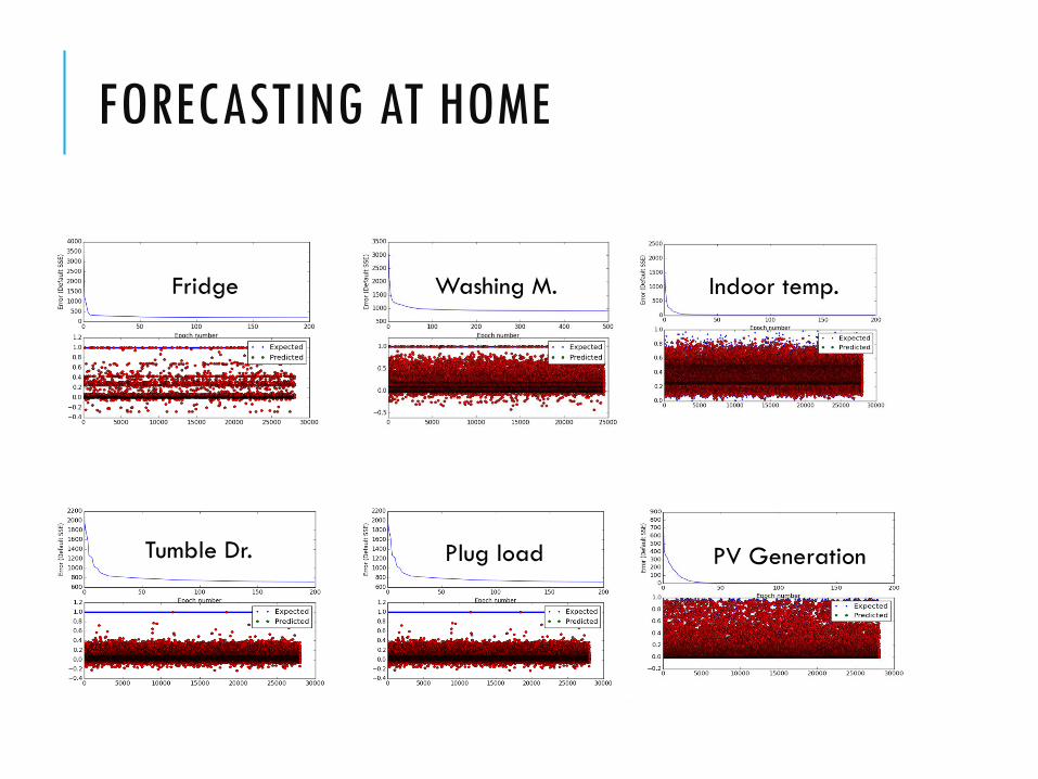
FORECASTING AT HOME
a) The training results of the best performed ANN for the demand of Device 1.
b) The training results of the best performed ANN for the demand of Device 2.
c) The training results of the best performed ANN for the
demand of Device 3.
d) The training results of the best performed ANN for the
demand of Device 4.
e) The training results of the best performed ANN for the Indoor Air Temperature.
f) The training results of the best performed ANN for the PV electricity generation.
Fridge
Tumble Dr.
Washing M.
Plug load PV Generation
Indoor temp.

RESULTS
25% reduction scenario10% reduction scenario
Original
Optimised
Original
Optimised

WIND POWER FORECASTING
0
5
10
15
20
25
30
0
1000
2000
3000
4000
5000
6000
7000
8000
304 305 306 307 308 309 310 311 312 313 314 315 316 317 318 319 320 321 322 323 324
ave watts
max watts
ave m/s
max m/s
0
1000
2000
3000
4000
5000
6000
7000
8000
0 1 2 3 4 5 6 7 8 9 10 11 12 13 14 15 16 17 18
wind m/s
power curve
Cp=0.4
power 240-260 compass
leaflet power
power 210-140 compass
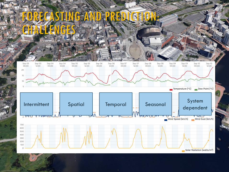
FORECASTING AND PREDICTION: CHALLENGES
Intermittent Spatial Temporal SeasonalSystem
dependent

URBAN AREA FORECASTING - 2
Figure 3 The labels and lcation of the building corners
on Quickbird (0.6 GSD) test image
Figure 4 (a) 3D visualisation of solar angles: Sun
Elevation, Azimuth and Zenith angle with the
formation of a cast shadow of the urban structure, (b)
a shadow pattern of the actual illumination direction
and its opposite direction, which is composed of the
cast direction of the shadow with the geometric angles
of the relationships within the image space
THE EVALUATION OF THE 3D MODEL
OF URBAN STRUCTURES
To evaluate and test the uncertainty in the creation of
a 3D model of detached buildings, we investigated the
area of the base (building footprint) of a 3D solid box
(which is also the same area of the top of a 3D model).
The shape of the buildings mostly represents a
rectangle shape, and therefore the area must be a
regular rectangular shape. This means the geometry of
the 3D solid boxes has right angles in each corner
between each of the two edges (in the 2D plan) within
the area of the base of the model. Accordingly, the
reference data (e.g. the shape of polygon) of each
building of test image was manually prepared by a
qualified human operator using ArcGIS and their areas
were calculated. Essentially, the reference data is the
data that was derived from high precision
measurements of their field measurements or aerial
photography or satellite imagery with a high spatial
resolution, including a local coordinate system and
widely used for comparison. Thereafter, the
comparison was based on an object-based assessment
between two area values of the building footprints of
the reference and computed area values from the
created 3D model were conducted. The results of the
comparison are shown in figure 6, which presents
some discrepancies between the true and measured
values. These discrepancies between the base area of
the 3D model (measured value) and the building
footprint area of the reference of the geometric
building (true value) were taken into account and
corrected using Ecotect software.
Figure 5 3D model of urban structures results of the
proposed approach with different azimuth (Az) and
Elevation (El) of MATLAB visualisation, (a) 3D
buildings visualised by the top view, (b)
Comprehensive view Az:71 & El:28, (c) X-side view
Az:-20, El:36, (d) Y-side view Az:-66, El:36, (e) Back-
sight view Az:147, El:36, (f) Front-sight view Az:7,
El:36
ASSESSMENT OF SOLAR ENERGY
POTENTIAL
The verification of the correct geometry is
implemented for the 3D model of urban structures in
Figure 7a and the true sun path and shadows of
buildings in Figure 7b. We consider the climate data
to assess, simulate and analyse the solar radiation on
building roofs and surfaces in Ecotect software. The
assessment is performed in terms of simulation and
(a)
(b)
(a) (b)
(c) (d)
(e) (f)
calculation of the cumulative values of the incident
solar radiation and total monthly solar exposure in
Figure 8. The total cumulative solar radiation
calculation and simulation were implemented on all
surfaces (rooftops and walls) of buildings across every
month covering the entire year in different directions.
The goal behind this simulation is to calculate and
assess the availability of incident solar radiation
(insolation) on surfaces within our model. To achieve
this goal, we used the weather file of our study area in
Ankara, which was created based on hourly recorded
data. We also consider the overshadowing and shading
calculation for the geometry of the buildings and their
surroundings.
Table 1
Performance results of corner detection of buildings
from the VHR satellite image (Quickbird test image)
Table 2
Performance results of the estimation of buildings
heights from the VHR satellite image (test image)
No.
of
buildings
The
measured
value of
building
height (m)
The
estimated
value of
building
height (m)
Differences
M-E
(m)
1 3.70 3.40 0.30
2 4.80 5.10 -0.30
3 4.00 5.70 -1.70
4 5.60 5.60 0.00
5 4.00 4.10 -0.10
6 5.60 4.80 0.80
7 5.60 4.80 0.80
RMSE -0.20
Mean -0.029 Standard Deviation 0.79
RESULTS AND DICUSSION
We visualise the assessment of the solar energy
potential of urban structures, which are derived from
the Quickbird test image in Figure 9. The extraction of
the 3D model of urban structures demonstrates that
our approach can provide remarkable assessment and
quite representative results. The assessment of the
solar energy potential for rooftops and facades based
on the solar 3D model of urban structures using
Ecotect software provides an opportunity to carry out
a fair quantitative comparison.
Figure 5 Evaluation of the areas of the polygons of the
extracted 3D model of urban buildings and the
reference data. The correction was implemented to the
extracted areas of the 3D model based on restoring
the right angles at the intersection of two
perpendicular straight lines
Figure 6 (a) The modified geometry of the 3D model
of the detached buildings in Ecotect, (b) the setting of
the sun path and the cast shadows of the detached
buildings in Ecotect
Figure 7 Solar radiation assessment for urban
structures (a) in the same direction of the solar
radiation, (b) in the opposite direction of the solar
radiation
According to Figure 9, the results illustrate the
differences between the amount of solar radiation
received by buildings’ roofs and surfaces (walls). The
lower values of incident solar radiation were found
within the buildings’ facades in the north direction in
Figure 9a. The facades in the east and west directions
present convergent values of solar radiation whereas
the inconsistent values were observed within the
facades in the south direction. In contrast, the amount
of received solar radiation by rooftops was higher than
other surfaces which exhibits large values of
insolation due to the fact that the regions of the
rooftops were full exposed to sunlight in Figure 10. In
particular, because the selected study area lacks dense
vegetation cover, such as trees, they receive more
solar radiation and thus have less overshadowing
vegetation cover over the rooftops.
ID
Diff. of
Location
(Pixels)
Accu.
(%)
ID
Diff. of
Location
(Pixels)
Accu.
(%)
1 0 100 15 0 100
2 0 100 16 0 100
3 8.98 91.02 17 0 100
4 2.84 97.16 18 7.25 92.75
5 0 100 19 66.15 33.85
6 0 100 20 65.36 34.65
7 0 100 21 0 100
8 0 100 22 0 100
9 7.40 92.60 23 6.06 93.94
10 3.31 96.69 24 6.06 93.94
11 9.86 90.64 25 0 100
12 7.40 92.60 26 13.80 86.20
13 0 100 27 14.86 85.13
14 0 100 28 5.52 94.48
(b) (a)
(b) (a)
Images Geometry Prediction
Kadhim N, Mourshed M, Bray, M (2015)

THANK YOU


