nanoNS3: Simulating Bacterial Molecular Communication
Based Nanonetworks in Network Simulator 3
⇤
Yubing Jian a, Bhuvana Krishnaswamy a, Caitlin M. Austin b
A. Ozan Bicen a, Jorge E. Perdomo b, Sagar C. Patel b
Ian F. Akyildiz a, Craig R. Forest b and Raghupathy Sivakumar a
a School of Electrical and Computer Engineeringb George W. Woodruff School of Mechanical Engineering
Georgia Institute of Technology, Atlanta, GA, USA
ABSTRACTWe present nanoNS3, a network simulator for modeling Bac-terial Molecular Communication (BMC) networks. nanoNS3is built atop the Network Simulator 3 (ns-3). nanoNS3 isdesigned to achieve the following goals: 1) accurately andrealistically model real world BMC, 2) maintain high com-putational e�ciency, 3) allow newly designed protocols tobe implemented easily. nanoNS3 incorporates the channel,physical (PHY) and medium access control (MAC) layersof the network stack. The simulator has models that accu-rately represents receiver response, microfluidic channel loss,modulation, and amplitude addressing designed specificallyfor BMC networks. We outline the design and architectureof nanoNS3, and then validate the aforementioned featuresthrough simulation and experimental results.
KeywordsBMC Simulator, ns-3, Di↵usion-based Molecular Communi-cation, Experimental-based Simulator
1. INTRODUCTIONMolecular communication is an emerging field of com-
munication between nodes using chemical molecules. It isa multidisciplinary field with concepts from biology, chem-istry, information theory and communication used in tandemto develop molecular communication systems. The commu-nication between nodes can in turn trigger the developmentof sophisticated practical applications that require cooper-ation. The medium for the molecular communication andhence the transceivers di↵er based on the applications, envi-ronment, signals to be sensed, etc. In recent years, bacteriahave emerged as a promising candidate for molecular com-munication nodes or transceivers for biological applications.
⇤This work was supported in part by the National ScienceFoundation under grant CNS-1110947.
Permission to make digital or hard copies of all or part of this work for personal orclassroom use is granted without fee provided that copies are not made or distributedfor profit or commercial advantage and that copies bear this notice and the full cita-tion on the first page. Copyrights for components of this work owned by others thanACM must be honored. Abstracting with credit is permitted. To copy otherwise, or re-publish, to post on servers or to redistribute to lists, requires prior specific permissionand/or a fee. Request permissions from [email protected].
NANOCOM’16, September 28-30, 2016, New York, NY, USAc� 2016 ACM. ISBN 978-1-4503-4061-8/16/09. . . $15.00
DOI: http://dx.doi.org/10.1145/2967446.2967464
Engineered bacteria is used in toxicology to detect metals [1]and arsenic pollution [2]. In this work, we focus on molecu-lar communication with bacteria as transmitter and receivernodes.
There exist many works focusing on the theoretical anal-ysis of BMC. [3] analyzes theoretical limits of informationrate and [4–6] propose mathematical models for the channeland transceiver of BMC. Protocols and algorithms that aredesigned to improve the throughput performance of BMChave been studied in [7, 8]. BMC is a super-slow communi-cation mechanism [8] as it takes 10x to 100x of minutes persignal for the receiver response. Thus, using experimentalanalysis to validate the performance of each state-of-the-art algorithm is extremely time consuming. Also, exactlyreplicating the experimental setup for di↵erent algorithmsis di�cult. Thus, building a computer-based BMC simula-tor to analyze the performance of di↵erent BMC algorithmsis an important problem. In this work, we focus on buildinga network simulator atop ns-3, so that di↵erent algorithmscan be implemented in the simulator and the performance ofthose algorithms can be analyzed and compared with eachother. The easy-to-use layered approach of ns-3 has resultedin it becoming one of the most popular network simulators.
There have been other attempts to build molecular com-munication simulators [9–14]. Accurate modeling of receiverresponse is a key factor in the simulator. Existing simu-lators use a simplified approximation of receiver responsethus a↵ecting the accuracy of the simulation. A detailedanalysis of related work is presented in Section 2. Themajor contributions of this work are thus the following:1) An accurate bacterial receiver response module is builtin nanoNS3. The bacterial receiver response model is val-idated using experimental results. 2) A microfluidic chan-nel loss model is implemented in nanoNS3 with user-definedgeometries and properties. 3) A bit level communicationwith On-O↵ keying modulation scheme is implemented innanoNS3. 4) In nanoNS3, new attributes are added to anew node class in ns-3 to define a bacterial transmitter, abacterial receiver and channel parameters. 5) An ampli-tude addressing mechanism is built in nanoNS3. Based onthe current features in nanoNS3, it is easy to extend thefunctionality of nanoNS3 to incorporate other related BMCresearch. The current version of nanoNS3 is available tobe downloaded at: http://www2.ece.gatech.edu/research/GNAN/ns-allinone-3.24.zip.
The rest of the paper is organized as follows. In Section2, we discuss challenges in building a network simulator for
BMC networks and review existing molecular communica-tion simulators. In Section 3, we describe the architectureof nanoNS3 and in Section 4, we explain briefly the pro-tocols implemented in nanoNS3. Finally, in Section 5, wepresent performance results for nanoNS3, and in Section 6we present some conclusions.
2. BACKGROUND AND RELATED WORKExperimental analysis and verification of BMC networks
are time-consuming [8]. Receiver response to an input chem-ical signal takes few hundred minutes, and hence experi-mental verification of di↵erent algorithms is extremely timeine�cient. Also, since the receiver nodes are live bacteria,it is di�cult to replicate parameters across di↵erent experi-ments. Due to the complexity of the experimental setup andthe time involved, it is di�cult to vary di↵erent parameterslike channel characteristics or characteristics of the trans-mitted signal. A computer-based BMC simulator is thusnecessary to analyze the performance of new or state-of-the-art algorithms developed for BMC networks. The objectiveof nanoNS3 is thus to simulate BMC networks with genet-ically engineered bacterial transceivers in a microfluidic en-vironment. Based on the extensible property of nanoNS3,customized BMC related features can also be implementedin nanoNS3.
Implementing a molecular communication simulator withbacteria as transceivers has the following challenges. 1) Theresponse of a bacterial receiver to chemical molecules in-volves multiple processes [6] and is non-linear. Accuratemodeling of the receiver response is important to simulate amolecular communication network with bacterial transceivers.2) Due to the dynamic nature of the system, algorithms de-veloped for BMC networks di↵er from traditional communi-cation algorithms significantly. Implementing state-of-the-artprotocols is important and is not a trivial extension of thetraditional communication modules. 3) The simulator shouldhave high computational e�ciency in simulating large BMCnetworks and long packet sizes.
In this context, we have developed nanoNS3 that ad-dresses the challenges identified in building a BMC net-work simulator. nanoNS3 is built on top of ns-3, whichis a discrete event based simulator. A discrete event basedsimulator is best suited for simulating processes with longdelays. BMC networks are super-slow networks with verylong transmission delays. Thus, using ns-3 helps nanoNS3to be time e�cient. ns-3 borrows concepts from [15] focus-ing on building a scalable network simulator, so ns-3 is alsoequipped with good scalability performance. Therefore, wechoose to develop our BMC network simulator on top ofns-3 allowing us to address one of the challenges viz., simu-lation time e�ciency and simulating large networks. Someof the advantages of using ns-3 are as follows: 1) good com-putational e�ciency for large networks, and 2) open sourcedavailability and ease of extensibility that enable other usersto implement state-of-art algorithms as needed. nanoNS3 isdeveloped and validated using experiments that rely on ge-netically engineered bacteria in microfluidic environments.
Some of the existing simulators focus on the physical trans-mission and reception of molecules by simulating individualmolecules and tracking their propagation leading to timeine�cient simulation. In contrast, nanoNS3 simulates bit-level transmission and reception instead of molecular leveltransmission and reception. This leads to higher computa-
tional e�ciency. nanoNS3 is able to simulate how transmit-ted bits are modulated to pulses at transmitter side, and howthe concentration of molecules is propagated and attenuatedthrough a microfluidic channel. At receiver side, the biolog-ical response of how N-Acyl homoserine lactone (AHL) dif-fuses through the biofilm material and subsequently acrossthe bacteria membrane is simulated. Then, the receiver canidentify the ID of the transmitter based on the received con-centration. Afterwards, the receiver can demodulate the re-ceived concentration to recover the transmitted information.
There are several existing works focused on simulatingMolecular Communication (MC) [9–13]. These approachesvalidate their respective simulators using numerical analysisor purely simplified theoretical models. Thus, the simula-tors are not verified against real-life behaviors. NanoNSis built on top of Network Simulator 2 (ns-2), and it pro-vides various nanoscale communication paradigms based ona di↵usive MC channel [9]. This work only presents the de-tails of the channel layer, and it simulates the di↵usion andreception process using a single equation, which may notbe accurate in the practical situation. This work simulatesMC using molecules based approach, which is time consum-ing as the molecule scales (for practical cases, the size ofmolecules is immense). Also, this work is based on ns-2which is computationally ine�cient with regards to memoryusage and CPU utilization. Currently, ns-2 is not activelymaintained, and the most recent version of ns-2 was releasedin 2011. In [10], N3Sim is developed based on the di↵usionpropagation channel to model MC networks. N3Sim is builton a customized simulator. Using customized simulator islikely to lose the advantages of dedicated network simula-tors like ns-3 (e.g. scalability and computational e�ciency).Also, network layers higher than the PHY layer is absent inN3Sim. Nano-Sim developed in [11] is also built on top of ns-3, and it provides functions to model Electromagnetic (EM)wave based nanonetworks. Similar like our work, Nano-Simutilizes the framework and advantages of ns-3 to build EM-based nano simulator. The transmission/reception schemein Nano-Sim is orthogonal to the work in this paper. Thus,it is feasible to combine nanoNS3 with Nano-Sim, since theyare both implemented atop ns-3. Other than aforementionedMC simulators, [14] proposes a simulation framework thatis adaptable to any kind of nano bearer and [14] is also vali-dated using experimental analysis in [16], but it is developedusing a customized simulator. Thus, it is likely to lose theadvantages of dedicated network simulators. To the best ofour knowledge, nanoNS3 is the first BMC network simula-tor validated using experimental systems with both channelattenuation and modulation analysis.
3. NETWORK ARCHITECTUREnanoNS3 is developed atop ns-3 [17]. ns-3 is a discrete
event, open source and widely used network simulator forinternet systems, targeted primarily for research and edu-cational use (ns-3 is developed in C++ and python). ns-3is developed based on modules, and each individual mod-ule represents a protocol (e.g. TCP), a technology (e.g.WiFi) or an attribute of networks (e.g. mobility). It enableseasy and convenient upgrade of source code and triggers theease of extensibility in ns-3 by this modular implementationmethod. ns-3 is actively maintained and it is free softwareand licensed under GNU GPLv2 license. ns-3 has the bestoverall performance compared with other popular network
simulators [18]. E.g. ns-3 has the least memory usage forlarge scale network simulations compared with ns-2, OM-NeT++, JiST and SimPy. Implementing nanoNS3 in ns-3has the following major advantages: 1) open sourced avail-ability and ease of implementation for new algorithms, 2)high computational e�ciency for large scale networks, and3) supporting tools from ns-3 can be utilized directly (e.g.ns-3 logging and tracing systems).
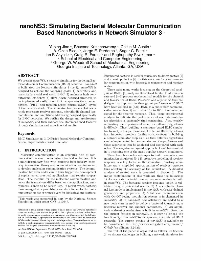
3.1 nanoNS3 Network ArchitectureThe high-level structure of nanoNS3 is shown in Fig. 1.
The name of seven important classes with the structure ofthe corresponding network layers are given in Fig. 1. Thefunctionality of each class is discussed briefly below:
• NanoNetDevice: It is similar to the Network InterfaceCard (NIC), and it can support di↵erent nano commu-nication technologies (e.g. di↵usive or EM wave basednano communication schemes) and corresponding pro-tocols (e.g. amplitude addressing).
• NanoNode: It can be regarded as the physical de-vice, and di↵erent NanoNetDevices can be integratedwith NanoNode to provide corresponding communica-tion technologies and protocols to enable NanoNode tocommunicate with each other.
• NanoMessage: This class is used to set up user de-fined applications for nano communications by control-ling application-related parameters, e.g., packet arriv-ing interval and packet size.
• NanoRouting : This class manages message forwardingby each NanoNode.
• NanoMAC : This class manages channel access of dif-ferent NanoNodes, and it also manages MAC layer ad-dressing mechanism.
• NanoPHY : This class is used to simulate the process oftransmitters and receivers to transmit and receive thenano signals. The corresponding functionality of thisclass includes modulation, demodulation and receiverresponse.
• NanoChannel : This class is used to set up channel con-ditions, and then the channel loss can be calculated tosimulate how the transmitted signals are propagatedand attenuated in the corresponding microfluidic chan-nel.
The parameters for each aforementioned class can be cus-tomized by users. Protocols implemented in NanoMAC,NanoPHY , and NanoChannel will be discussed in Section4.
4. PROTOCOLS IMPLEMENTEDnanoNS3 implements some of the basic protocols to simu-
late BMC networks. The important 4 models implementedin nanoNS3 are: 1) Receiver response model, 2) Channelloss model, 3) On-O↵ Keying model, and 4) Amplitude ad-dressing model.
Figure 1: nanoNS3 Architecture
4.1 Receiver Response ModelAs discussed in Section 2, accurate modeling of receiver
response is important to simulate BMC networks. nanoNS3focuses on simulating BMC networks and hence modeling ofresponse of bacteria to molecular signal is described in thissection. The bacterial receiver implemented in this simu-lator is a population of genetically engineered E. coli bac-teria that generates a Green Fluorescent Protein (GFP) onreceiving AHL molecules. The transceivers are located ina microfluidic device connected by microfluidic pathways.The transmitter transmits molecules that are transportedto the receiver through microfluidic pathways and the re-ceiver emits green fluorescence. The relative fluorescence ofthe receiver bacteria indicates the signal received. [6] reviewsthe existing bacterial receiver models in a microfluidic envi-ronment and proposes a new model. [6] validates the modelusing experiments. In nanoNS3, we implement the followingmodel proposed in [6].
dAHLi
dt= k
c
(AHLe
�AHLi
)�k1AHLi
2LuxR2+k1C1 (1)
dC1
dt= k1AHL
i
2LuxR2 � k1C1 � k2C2PLux
(2)
dC2
dt= k2C1PLux
� k2C2 � ktr
C2 (3)
dLuxR
dt= k
Lc
� 2C1 � 2C2 (4)
dGFPi
dt= k
tr
C2 � kGm
GFPi
� kGd
GFPi
(5)
dGFPm
dt= k
Gm
G+ i� kGd
GFPm
(6)
AHLe
and AHLi
are the external and internal concen-trations of molecules at the receiver. LuxR,C1, C2, andGFP
i
represent internal parameters of the receiver bacteria.

GFPm
represents the concentration of GFP which in turnrepresents the relative fluorescence at the receiver. Vectork = [k
c
, k1, k2, kLc
, ktr
, kGd
, kGm
] represents rate constantsof the processes in the receiver. The equations and corre-sponding derivation are explained in detail in [6].
The above equations are used to model the channel andreceiver response in nanoNS3. The transmitter module gen-erates bits and those bits are input to the modulator andchannel model followed by these equations to simulate theGFP response of the receiver. A numerical inverse of theseequations is used to sample and quantize the received signalwhich is then fed to the demodulator to process. This modelgives a bit level response of the receiver.
4.2 Channel Loss ModelMicrofluidic channel loss model is an important compo-
nent for BMC simulators, which provides insights for howconcentration signals are attenuated while propagating inmircrofluidic channel. [5] provides a comprehensive cover-age of the microfluidic channels with fluid flow for di↵usion-based Flow-induced Molecular Communication (FMC). InFMC, the fluid is flowing through a microfluidic channel andit serves as a communication channel to connect patches ofmolecular transmitter and receiver, such as bacterial habi-tat. In [5], an analytic study of the propagation of themolecules in the form of impulse response is performed in-corporating the physical system parameters. The goal ofthe propagation loss model is to determine the channel losse↵ects caused on the molecular signal with respect to thedistance, fluid flow parameters (pressure drop, flow velocity,microfluidic channel geometry and fluid type), and type ofthe molecule (di↵usion constant). In [5], channel loss mod-els for the basic microfluidic channel shapes (straight andturning) and cross-sections (rectangular, square, elliptical,circular) are developed incorporating the characteristics ofthe fluid flow and mass transport in the microfluidic chan-nels. In nanoNS3, we implement the models presented in [5].In the interest of brevity, we will illustrate rectangular cross-section microfluidic channel loss model in this section, andevaluate the specific microfluidic channel loss model in Sec-tion 5. The governing set of equations for the channel lossin a rectangular microfluidic channel are given as [5].
Grect
=h3w
12µl⇤ (1� 0.63
h
w) (7)
urect
= Grect
⇤ 4p (8)
⌧rect
= l/urect
(9)
TFrect
= e�(k2D+jkurect)⇤⌧rect (10)
where Grect
, urect
are the hydraulic conductance of themicrofluidic channel and area-averaged flow rate, respec-tively. G
rect
is a function of channel cross-section shape,dimensions, and viscosity of the fluid (µ). u
rect
is a functionof pressure drop (4p) and G
rect
. ⌧rect
and TFrect
are thedelay and attenuation of channel, respectively. h and w rep-resent the channel height and width. l and D are the lengthof the straight channel and Taylor dispersion-adjusted di↵u-sion constant. The detailed explanations for all microfluidicchannel loss models are given in [5].
4.3 On-Off Keying (OOK) ModelModulation is the process of varying the properties of a
signal to convey the information. Modulation determinesthe rate of transmission. ns-3 allows users to change mod-ulation by changing the transmission rate. In nanoNS3, weimplement bit level simulation and hence implement a mod-ule for modulation. OOK is one of the simplest modulationtechniques and majority of works on BMC assume OOKas the modulation technique. OOK transmits a rectangu-lar pulse of amplitude/concentration A for a duration of T1
time units to send bit 1 and no signal for T2 time units tosend bit 0. OOK module in nanoNS3 generates a rectangu-lar pulse of a given amplitude and a given duration. Then,the generated rectangular pulse is fed to the channel model.
4.4 Amplitude Addressing ModelThe models mentioned above (receiver response, channel
loss and OOK) model the channel and physical layer of BMCnetworks. A MAC protocol is required in a network withmultiple sources to achieve fairness and reduce collisions.MAC protocols used in wired or wireless networks as imple-mented in ns-3 increase the delay and decrease the through-put in a super-slow network like the BMC network. [7] con-siders a multiple sources and single receiver topology andproposes a MAC protocol to improve the BMC networkthroughput. Multiple sources transmitting to a single re-ceiver is a typical sensing network scenario. [7] proposes alocal addressing mechanism which implicitly performs MAC,and it is implemented in nanoNS3. [7] analyses the advan-tages and disadvantages of various addressing mechanismsand proposes Amplitude Addressing for BMC networks. Am-plitude Addressing assigns distinct amplitudes to each userin a BMC network and each user uses the assigned ampli-tude with OOK to transmit information. The receiver re-ceives the sum of the transmitted amplitudes which are thenresolved to identify the individual amplitude thus solving ad-dressing and MAC in the local network. A global address isrequired to map local address to the source. nanoNS3 doesnot have a global addressing module, but MAC address ofns-3 nodes can be used as a global address module in simu-lations.
5. RESULTSIn this section, we present the evaluation results of nanoNS3
using both simulation-based and experimental-based valida-tion for the 4 models mentioned in Section 4. nanoNS3provides two examples of scenario setup: 1) single Tx andsingle Rx, and 2) multiple Txs and single Rx.
5.1 MethodologyIn this section, we validate nanoNS3 with protocols men-
tioned in Section 4. For the receiver response model, wevalidate the simulation results of nanoNS3 with results fromMATLAB analytic model used in [6] and experiments. Foramplitude addressing model, we validate nanoNS3 with pythonsimulator used in [7]. For channel loss model, we validatenanoNS3 with MATLAB analytical model used in [5]. Un-less otherwise mentioned, the transceivers used are bacteriaand the carrier signal is a molecular signal. To validate theperformance of the aforementioned models in nanoNS3, thefollowing scenarios are used:
• Single Tx and single Rx scenario: It is a single link
Table 1: Simulation Parameters for Receiver Response
Parameters Default SettingsTx sequence 1000100010Modulation OOK
Tx pulses amplitude 15 µMTx pulses width 50min
threshld 7.5µMkc
254/60kGm
1.8/60kGd
39/60ktr
1334/60kLc
1200/60k1 20/60k2 200/60
scenario where one transmitter sends signals to onereceiver. The default transmitted molecular concen-tration is set as 15 µM.
• Multiple Txs and single Rx scenario: Multiple trans-mitters send signals to a single receiver in this scenario.The amplitude assigned to each transmitter is based onthe mechanisms shown in [7], and two examples will begiven in Section 5.4.
5.2 Receiver ResponseWe implement the receiver response model derived in [6].
The set of di↵erential equations presented in [6] defines theGFP response of the receiver bacteria to a given concentra-tion of molecules. We built an Inverse model of the receiverresponse at the receiver to estimate the molecules receivedfrom the receiver GFP response.
We validate nanoNS3 receiver response in two steps. First,we verify the numerical inverse response using simulations.A transmitter sends information using OOK, i.e. rectangu-lar pulses of a fixed amplitude and a fixed duration for bit 1and no signal for bit 0. The rectangular pulses are input toForward response generating receiver GFP response whichis then fed to Inverse response derived numerically that es-timates the signal transmitted based on the GFP response.Second, we compare the forward receiver response obtainedfrom simulator with the response from experiments. We alsoinput the receiver response from experiments to the Inversemodel and compare the estimated signal with the actualtransmitted signal.
5.2.1 Receiver response : simulation validationIn this section, we validate the inverse receiver response
model using OOK. Fig. 2a and Fig. 2b present the trans-mitted and received rectangular pulses for the input bits andforward receiver response, respectively. The correspondingsimulation parameters are shown in Table 1. As we cansee from Fig. 2a, the transmitted rectangular pulses ex-actly match the received rectangular pulses. This result il-lustrates that the receiver can recover the transmitted pulsesin nanoNS3. The corresponding forward receiver responsefor the transmitted rectangular pulses is given in Fig. 2b.
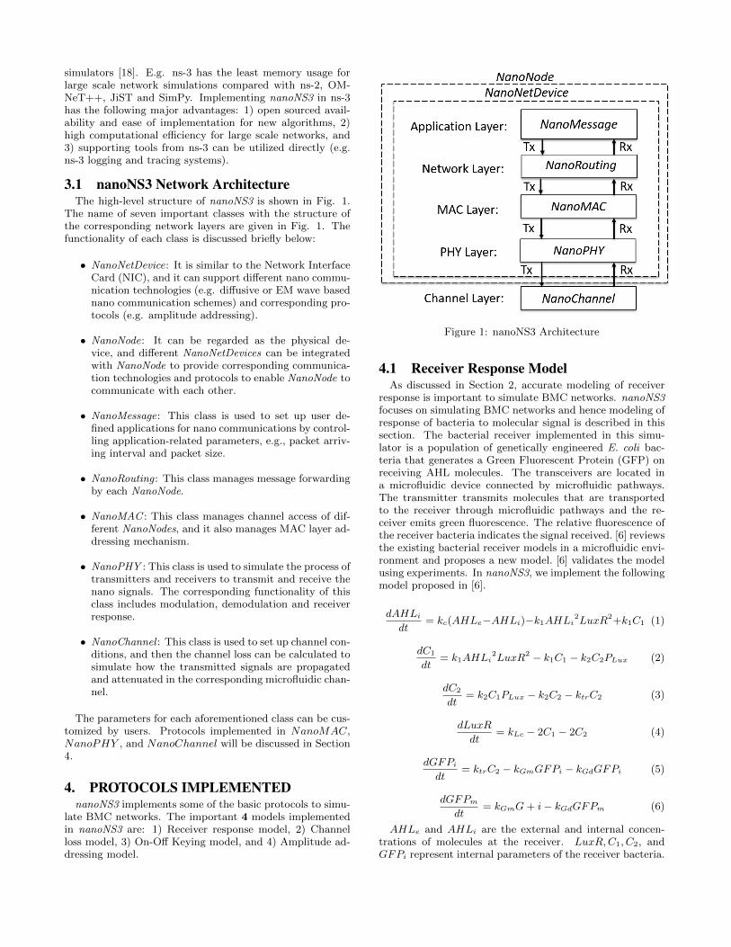
5.2.2 Receiver response : experimental validationIn this section, we validate the receiver response model us-
ing experimental results. Experimental setup used to obtainthese results are the same as explained in [6]. We compare
0 500 1000 1500
0
2
4
6
810
12
14
16
18
Time (minute)
Co
nce
ntr
atio
n (
μM
)
Transmitted rectangular pulses
Received rectangular pulses
(a) Tx/Rx pulses comparison
0 500 1000 1500
0
5
10
15
20
25
30
Time (minute)
Re
lati
ve f
luo
rese
nce
(U
A)
(b) Forward receiver response
Figure 2: Simulation Validation
0
5
10
15
20
0 500 1000 1500
Co
nse
ntr
atio
n (μM
)
Time (minute)
(a) Experimental Tx pulses
0
5
10
15
20
25
30
0 500 1000 1500
Rel
ativ
e fl
uo
rese
nce
(A
U)
Time (minute)
Experimental validation
Simulation
(b) Forward receiver response
Figure 3: Experimental Validation
the receiver response obtained from experiments and sim-ulations. We also verify the inverse of receiver response.The receiver response from experiments is input to the in-verse model and we compare the estimated transmitted sig-nal with the actual transmitted signal.
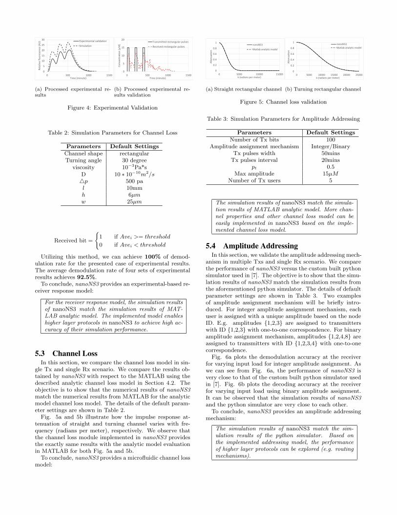
Forward receiver response validationFig. 3a presents the transmitted rectangular pulses. Fig.3b shows the simulation results and experimental results ofthe forward receiver response. It can be observed that thesimulation and experimental results have the similar trends(peaks of each pulse in experimental results can be exactlycaptured by simulation). Four di↵erent Tx sequences with10 bits in each sequence are set as Tx sequence in the ex-perimental apparatus, and each of them shows the similartrend as the presented results.
Inverse receiver response validationBased on the experimental results of forward receiver re-sponse, we validated the inverse of the receiver response.From Fig. 3b, it is clear that experimental results of forwardreceiver response is not as smooth as the simulation resultsof forward receiver response. In order to get rid of noisesand system errors, we use Loess smooth function (with 10%span) in MATLAB to smooth the experimental results. Thecorresponding experimental results are shown in Fig. 4a.Then, we input those smoothed experimental results to theinverse of receiver response model in nanoNS3, and we suc-ceeded to recover the transmitted bits at the receiver side.From Fig. 4b, it can be observed that the peaks of trans-mitted and received pulses match with each other. In orderto demodulate the received pulses, we calculate the aver-age concentration for the pulse duration of each bit, whereaverage concentration for bit i is represented as Ave
i
. Weset a threshold to determine the bit level, where thresholdis set as half of transmitted concentration. Received bit isdetermined by the following equation:
0
5
10
15
20
25
30
0 500 1000 1500
Rel
ativ
e fl
uo
rese
nce
(A
U)
Time (minute)
Experimental validation
Simulation
(a) Processed experimental re-
sults
0
5
10
15
20
0 500 1000 1500
Co
nse
ntr
atio
n (μM
)
Time (minute)
Transmitted rectangular pulses
Received rectangular pulses
(b) Processed experimental re-
sults validation
Figure 4: Experimental Validation
Table 2: Simulation Parameters for Channel Loss
Parameters Default SettingsChannel shape rectangularTurning angle 30 degree
viscosity 10�3Pa*sD 10 ⇤ 10�10m2/s4p 500 pal 10mmh 6µmw 25µm
Received bit =
(1 if Ave
i
>= threshold
0 if Avei
< threshold
Utilizing this method, we can achieve 100% of demod-ulation rate for the presented case of experimental results.The average demodulation rate of four sets of experimentalresults achieves 92.5%.
To conclude, nanoNS3 provides an experimental-based re-ceiver response model:
For the receiver response model, the simulation resultsof nanoNS3 match the simulation results of MAT-LAB analytic model. The implemented model enableshigher layer protocols in nanoNS3 to achieve high ac-curacy of their simulation performance.
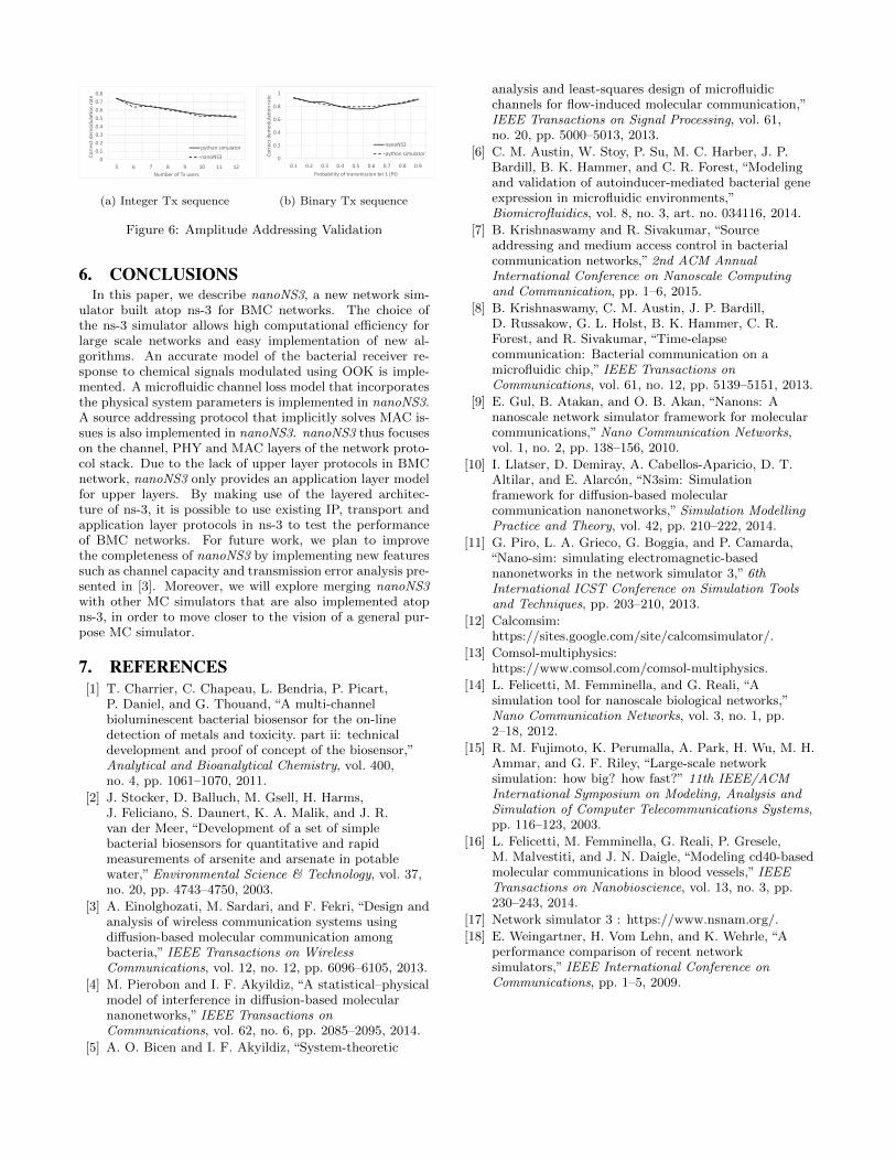
5.3 Channel LossIn this section, we compare the channel loss model in sin-
gle Tx and single Rx scenario. We compare the results ob-tained by nanoNS3 with respect to the MATLAB using thedescribed analytic channel loss model in Section 4.2. Theobjective is to show that the numerical results of nanoNS3match the numerical results from MATLAB for the analyticmodel channel loss model. The details of the default param-eter settings are shown in Table 2.
Fig. 5a and 5b illustrate how the impulse response at-tenuation of straight and turning channel varies with fre-quency (radians per meter), respectively. We observe thatthe channel loss module implemented in nanoNS3 providesthe exactly same results with the analytic model evaluationin MATLAB for both Fig. 5a and 5b.
To conclude, nanoNS3 provides a microfluidic channel lossmodel:
0
0.2
0.4
0.6
0.8
1
0 5000 10000 15000
Att
enu
atio
n
k (radians per meter)
nanoNS3
Matlab analytic model
(a) Straight rectangular channel
0
0.2
0.4
0.6
0.8
1
0 5000 10000 15000 20000 25000
Att
enu
atio
n
k (radians per meter)
nanoNS3
Matlab analytic model
(b) Turning rectangular channel
Figure 5: Channel loss validation
Table 3: Simulation Parameters for Amplitude Addressing
Parameters Default SettingsNumber of Tx bits 100
Amplitude assignment mechanism Integer/BinaryTx pulses width 50minsTx pulses interval 20mins
pt
0.5Max amplitude 15µM
Number of Tx users 5
The simulation results of nanoNS3 match the simula-tion results of MATLAB analytic model. More chan-nel properties and other channel loss model can beeasily implemented in nanoNS3 based on the imple-mented channel loss model.
5.4 Amplitude AddressingIn this section, we validate the amplitude addressing mech-
anism in multiple Txs and single Rx scenario. We comparethe performance of nanoNS3 versus the custom built pythonsimulator used in [7]. The objective is to show that the simu-lation results of nanoNS3 match the simulation results fromthe aforementioned python simulator. The details of defaultparameter settings are shown in Table 3. Two examplesof amplitude assignment mechanism will be briefly intro-duced. For integer amplitude assignment mechanism, eachuser is assigned with a unique amplitude based on the nodeID. E.g. amplitudes {1,2,3} are assigned to transmitterswith ID {1,2,3} with one-to-one correspondence. For binaryamplitude assignment mechanism, amplitudes {1,2,4,8} areassigned to transmitters with ID {1,2,3,4} with one-to-onecorrespondence.
Fig. 6a plots the demodulation accuracy at the receiverfor varying input load for integer amplitude assignment. Aswe can see from Fig. 6a, the performance of nanoNS3 isvery close to that of the custom built python simulator usedin [7]. Fig. 6b plots the decoding accuracy at the receiverfor varying input load using binary amplitude assignment.It can be observed that the simulation results of nanoNS3and the python simulator are very close to each other.
To conclude, nanoNS3 provides an amplitude addressingmechanism:
The simulation results of nanoNS3 match the sim-ulation results of the python simulator. Based onthe implemented addressing model, the performanceof higher layer protocols can be explored (e.g. routingmechanisms).
0
0.1
0.2
0.3
0.4
0.5
0.6
0.7
0.8
5 6 7 8 9 10 11 12
Co
rrec
t d
em
od
ula
tio
n r
ate
Number of Tx users
python simulator
nanoNS3
(a) Integer Tx sequence
0
0.2
0.4
0.6
0.8
1
0.1 0.2 0.3 0.4 0.5 0.6 0.7 0.8 0.9
Co
rre
ct d
em
od
ula
tio
n r
ate
Probability of transmission bit 1 (Pt)
nanoNS3
python simulator
(b) Binary Tx sequence
Figure 6: Amplitude Addressing Validation
6. CONCLUSIONSIn this paper, we describe nanoNS3, a new network sim-
ulator built atop ns-3 for BMC networks. The choice ofthe ns-3 simulator allows high computational e�ciency forlarge scale networks and easy implementation of new al-gorithms. An accurate model of the bacterial receiver re-sponse to chemical signals modulated using OOK is imple-mented. A microfluidic channel loss model that incorporatesthe physical system parameters is implemented in nanoNS3.A source addressing protocol that implicitly solves MAC is-sues is also implemented in nanoNS3. nanoNS3 thus focuseson the channel, PHY and MAC layers of the network proto-col stack. Due to the lack of upper layer protocols in BMCnetwork, nanoNS3 only provides an application layer modelfor upper layers. By making use of the layered architec-ture of ns-3, it is possible to use existing IP, transport andapplication layer protocols in ns-3 to test the performanceof BMC networks. For future work, we plan to improvethe completeness of nanoNS3 by implementing new featuressuch as channel capacity and transmission error analysis pre-sented in [3]. Moreover, we will explore merging nanoNS3with other MC simulators that are also implemented atopns-3, in order to move closer to the vision of a general pur-pose MC simulator.
7. REFERENCES[1] T. Charrier, C. Chapeau, L. Bendria, P. Picart,
P. Daniel, and G. Thouand, “A multi-channelbioluminescent bacterial biosensor for the on-linedetection of metals and toxicity. part ii: technicaldevelopment and proof of concept of the biosensor,”Analytical and Bioanalytical Chemistry, vol. 400,no. 4, pp. 1061–1070, 2011.
[2] J. Stocker, D. Balluch, M. Gsell, H. Harms,J. Feliciano, S. Daunert, K. A. Malik, and J. R.van der Meer, “Development of a set of simplebacterial biosensors for quantitative and rapidmeasurements of arsenite and arsenate in potablewater,” Environmental Science & Technology, vol. 37,no. 20, pp. 4743–4750, 2003.
[3] A. Einolghozati, M. Sardari, and F. Fekri, “Design andanalysis of wireless communication systems usingdi↵usion-based molecular communication amongbacteria,” IEEE Transactions on WirelessCommunications, vol. 12, no. 12, pp. 6096–6105, 2013.
[4] M. Pierobon and I. F. Akyildiz, “A statistical–physicalmodel of interference in di↵usion-based molecularnanonetworks,” IEEE Transactions onCommunications, vol. 62, no. 6, pp. 2085–2095, 2014.
[5] A. O. Bicen and I. F. Akyildiz, “System-theoretic
analysis and least-squares design of microfluidicchannels for flow-induced molecular communication,”IEEE Transactions on Signal Processing, vol. 61,no. 20, pp. 5000–5013, 2013.
[6] C. M. Austin, W. Stoy, P. Su, M. C. Harber, J. P.Bardill, B. K. Hammer, and C. R. Forest, “Modelingand validation of autoinducer-mediated bacterial geneexpression in microfluidic environments,”Biomicrofluidics, vol. 8, no. 3, art. no. 034116, 2014.
[7] B. Krishnaswamy and R. Sivakumar, “Sourceaddressing and medium access control in bacterialcommunication networks,” 2nd ACM AnnualInternational Conference on Nanoscale Computingand Communication, pp. 1–6, 2015.
[8] B. Krishnaswamy, C. M. Austin, J. P. Bardill,D. Russakow, G. L. Holst, B. K. Hammer, C. R.Forest, and R. Sivakumar, “Time-elapsecommunication: Bacterial communication on amicrofluidic chip,” IEEE Transactions onCommunications, vol. 61, no. 12, pp. 5139–5151, 2013.
[9] E. Gul, B. Atakan, and O. B. Akan, “Nanons: Ananoscale network simulator framework for molecularcommunications,”Nano Communication Networks,vol. 1, no. 2, pp. 138–156, 2010.
[10] I. Llatser, D. Demiray, A. Cabellos-Aparicio, D. T.Altilar, and E. Alarcon, “N3sim: Simulationframework for di↵usion-based molecularcommunication nanonetworks,” Simulation ModellingPractice and Theory, vol. 42, pp. 210–222, 2014.
[11] G. Piro, L. A. Grieco, G. Boggia, and P. Camarda,“Nano-sim: simulating electromagnetic-basednanonetworks in the network simulator 3,” 6thInternational ICST Conference on Simulation Toolsand Techniques, pp. 203–210, 2013.
[12] Calcomsim:https://sites.google.com/site/calcomsimulator/.
[13] Comsol-multiphysics:https://www.comsol.com/comsol-multiphysics.
[14] L. Felicetti, M. Femminella, and G. Reali, “Asimulation tool for nanoscale biological networks,”Nano Communication Networks, vol. 3, no. 1, pp.2–18, 2012.
[15] R. M. Fujimoto, K. Perumalla, A. Park, H. Wu, M. H.Ammar, and G. F. Riley, “Large-scale networksimulation: how big? how fast?” 11th IEEE/ACMInternational Symposium on Modeling, Analysis andSimulation of Computer Telecommunications Systems,pp. 116–123, 2003.
[16] L. Felicetti, M. Femminella, G. Reali, P. Gresele,M. Malvestiti, and J. N. Daigle, “Modeling cd40-basedmolecular communications in blood vessels,” IEEETransactions on Nanobioscience, vol. 13, no. 3, pp.230–243, 2014.
[17] Network simulator 3 : https://www.nsnam.org/.[18] E. Weingartner, H. Vom Lehn, and K. Wehrle, “A
performance comparison of recent networksimulators,” IEEE International Conference onCommunications, pp. 1–5, 2009.


