
Comput Methods Biomech Biomed Engin. 2011 Apr 1:1. [Epub ahead of print]
Left ventricular wall stress compendium
L. Zhong1*, D.N. Ghista2, R.S. Tan1
1Department of Cardiology, National Heart Centre Singapore, Mistri Wing 17 Third Hospital Avenue Singapore 1687522Framingham State University, Framingham, Massachusetts, 01701-9101, USA
Correspondence: Dr. Liang Zhong, Department of Cardiology, National Heart Centre Singapore, Mistri Wing 17 Third Hospital Avenue, 168752. Email: z hong [email protected] ; Phone : +65 64367684Fax: +65 62230972 (Received xx Dec 2010; final version received xxx)
Left Ventricular wall stress has intrigued scientists and cardiologists since the time of Lame and Laplace in 1800 (s). The LV is an intriguing organ structure, whose intrinsic design enables it to fill and then contract to eject blood into the aorta. The development of wall stress is then also intriguing to cardiologists and biomedical engineers working in cardiology. The role of LV wall stress in cardiac perfusion and pumping as well as in cardiac pathophysiology is a relatively unexplored phenomenon. But even for us to assess this role, we first need accurate determination of in vivo wall stress. However, at this point, 150 years after Lame estimated LV wall stress using elasticity theory, we are still in the exploratory stage of (i) developing LV models that properly represent LV anatomy and physiology, and (ii) obtaining data on LV dynamics during the cardiac cycle. In this paper, we are responding to the need for a comprehensive survey of LV wall stress models, their mechanics, stress computation, and results. We have provided herein a compendium of major type of wall stress models: thin wall models based on Laplace Law, thick wall shell models, elasticity theory dynamic shape model, thick-wall large deformation models, and finite element models. We have compared the mean stress values of these models as well as the variation of stress across the wall. All of the thin-wall and thick-wall shell models are based on idealized ellipsoidal and spherical shaped geometries. However, the elasticity model’s shape can vary through the cycle, to simulate the more ellipsoidal shape of the LV in the systolic phase. The finite element models have more representative geometries, but are generally based on animal data, which limits their medical relevance. This paper can enable readers to obtain a comprehensive perspective of LV wall stress models, of how to employ them to determine wall stresses, and be cognizant of the assumptions involved in the use of specific models.
Keywords: left ventricular wall stress; shell model, elasticity, large-deformation, finite element model, cardiac mechanics
1. IntroductionIt all started with two great cardiologists Dr Hal Sandler and Dr Harold Dodge
publishing their pioneering paper on left ventricular tension and stress in man in
Circulation Research (1963). This phenomenal paper stirred a huge amount of activity
and enquiry into left ventricular wall stress. As a result, by 1969, three more
1

pioneering works were published by Wong and Rautanharju (1968), Ghista and
Sandler (1969) and Mirsky (1969). From thereon, this activity has kept burgeoning
until today. So, let us recognize and pay tribute to the pioneers Dr Sandler and Dr
Dodge, as we embark on the exotic trail of LV wall stress.
Cardiologist and physiologists has long been interested in quantification of left
ventricular (LV) wall stress. This is because: (1) wall stress has been viewed as an
important stimulus for the remodeling of the failing heart (Mann, 2004; Zhong et al.,
2009); (2) wall stress is one of the determinants of myocardial oxygen consumption
and plays an important role in the mechanical behaviour of the coronary circulation
(Jan et al., 1985); (3) wall stress contributes to adverse consequences for energy
metabolism, gene expression, and arrhythmia risk (Schwitter et al., 1992; Di Napoli et
al., 2003; Alter et al., 2008); (4) Wall stress triggers hypertrophy (Grossman et al.,
1980). Hence, the level and distribution of wall stress and its cyclic variation provide
a quantitative evaluation of the response and adjustment of the LV to heart disease.
The joint use of imaging and modeling of the heart has opened up possibilities
for a better thorough understanding and evaluation of the LV wall stress (see, for
instance, the Physiome Project (Smith et al., 2002; Hunter et al., 2003; Crampin et al.,
2004)). However, still due to the limitations of medical imaging and modeling
capabilities, the application of heart models to employ human in vivo data for their
use in clinical applications still remains a challenge which this paper attempts to
address.
Traditionally, most works on LV wall stress have been based on two- and
three-dimensional models that are represented by simplified idealized geometry
analyses (e.g., a sphere, spheroid, or ellipsoid is used to approximate the shape of the
ventricle) (Wong et al., 1968; Ghista & Sandler 1969; Mirsky et al., 1969; Moriarty
2

1980). The accuracy of these simplified geometry models is compromised because of
the complex geometrical shapes and deformations of the left ventricle (Gould et al.,
1972; Solomon et al., 1998). Finite element analysis (FEA), an engineering technique
utilized to study complex structures, can overcome some of these limitations (Ghista
et al. 1977; Janz 1981; Guccinone et al. 1995; Bovendeerd et al. 1996; Costa et al.
1996). Research in the last two decades has elucidated characteristics of LV wall
stress, and clarified how they should be properly analyzed so that these concepts can
be applied in translational research (Guccione et al., 2003; Dang et al., 2005; Walker
et al., 2005; Wall et al., 2006; Walker et al., 2008).
From the clinical applications consideration, the assessment and relevance of
LV wall stress in heart failure (HF) has been studied by using angiography (Sandler &
Dodge 1963; Ghista et al., 1977; Pouleur et al.,1984; Hayashida et al., 1990),
echocardiography (Douglas et al; 1987; Feiring et al., 1992; Turcani et al., 1997;
Rohde et al., 1999; de Simone et al., 2002) and cardiac magnetic resonance imaging
(MRI) (Fujita et al., 1993; Balzer et al., 1999; Delepine et al., 2003; Prunier et al.,
2008; Zhong et al., 2009). In this regard, due to the different imaging modalities,
some differences may occur in the data on LV geometry. However, most importantly,
in order to properly bring to bear the clinical application of LV wall stress, we also
need a clear understanding of theories and analyses of LV wall stress.
Even, direct measurement of wall force in the intact heart using various types
of strain gauge transducers coupled directed to the myocardium has been attempted
over the years (Hefner et al., 1962; Huisman et al., 1980). Some of the limitations
(e.g., insertion of transducer damages the tissue) and problems associated with these
direct measurement techniques have been extensively discussed by Huisman et al.
(1980). They have demonstrated that much of the uncertainty in the measured values
3

of wall stress was related to the degree of coupling between the transducer and the
muscle wall.
This paper will focus on: (1) biomechanical analyses, analytical and
computational models used to characterize LV wall stress, along with (2) clinical
methods available for monitoring in vivo data to determine LV wall stress. Herein, we
will present the available methods for calculating ventricular wall stress and provide
the reader with enough information to allow evaluation of the trade-off in accuracy
between simplified models and more representative models for the purpose of clinical
evaluation and applications of LV wall stress.
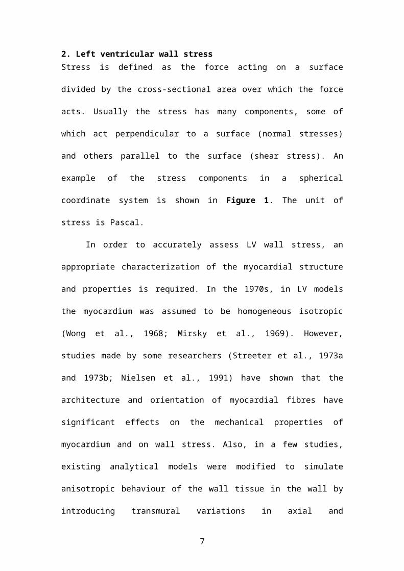
2. Left ventricular wall stressStress is defined as the force acting on a surface divided by the cross-sectional area
over which the force acts. Usually the stress has many components, some of which act
perpendicular to a surface (normal stresses) and others parallel to the surface (shear
stress). An example of the stress components in a spherical coordinate system is
shown in Figure 1. The unit of stress is Pascal.
In order to accurately assess LV wall stress, an appropriate characterization of
the myocardial structure and properties is required. In the 1970s, in LV models the
myocardium was assumed to be homogeneous isotropic (Wong et al., 1968; Mirsky et
al., 1969). However, studies made by some researchers (Streeter et al., 1973a and
1973b; Nielsen et al., 1991) have shown that the architecture and orientation of
myocardial fibres have significant effects on the mechanical properties of
myocardium and on wall stress. Also, in a few studies, existing analytical models
were modified to simulate anisotropic behaviour of the wall tissue in the wall by
introducing transmural variations in axial and circumferential stiffness of the material
(Misra et al., 1985).
4

Figure 1 Stress concept, illustrating the principal directions and corresponding
normal wall stress components in the spherical coordinates system. For the wall
element, R is the meridional radius of curvature and r is the circumferential radius of
curvature. This figure is adopted from Yin et al., Ventricular wall stress. Circ Res;
1981;49:829-841.
Myocardial properties include passive and active components. One of the
simplest approaches for deriving the passive material properties of the myocardium is
the uniaxial tension test. However, due to the three-dimensional constitutive
behaviour of the myocardium, uniaxial stress-strain data are insufficient for the
purpose (Costa et al., 2001). Triaxial testing is considered as the ideal approach, but it
remains a challenging and difficult practice. It is thus the common practice for
researchers (Yin et al., 1987; Huyghe et al., 1991; Nielsen et al., 1991) to characterize
myocardial material properties by biaxial tissue testing. In general, for its constitutive
behaviour, the myocardium is assumed to be hyperelastic with the strain energy
density function formulated from biaxial experimental data. Based on this
consideration, researchers have come up with different constitutive laws to describe
5

the passive myocardial behaviour (Guccoine et al, 1991; Humphrey et al., 1990;
Hunter et al; 1997; Vetter et al., 2000).
Active muscle constitutive law is a relation between stress and strain-rate, and
is based on the sarcomere model of series elastic element, parallel elastic element and
contractile element, which is based on interaction between the actin and myosin
filaments. Many constitutive laws have been proposed, including Hill’s three-
component model (Hill et al., 1950), Huxley’s sliding-filament model (Huxley et al.,
1957), Hunter’s fading memory model (Hunter et al) and Bestel-Clement-Sorine
(BCS) model (Bestel et al., 2001; Arts et al., 2001; Costa et al., 2001; Hunter et al.,
2003) and mechatronic sarcomere contractile model (Ghista et al. 2005). However, up
till now, there is still somewhat lack of reliable constitutive laws to describe the active
properties of the myocardium during the systolic phase.
First paragraph style
2.1 Left ventricular wall stress formulations by Laplace LawDespite its simplicity, the Laplace Law has been widely accepted by many
investigators. With the simultaneous measurement of LV pressure and geometry, it is
possible to quantify LV wall stress. Laplace derived the relationship relating the
pressure inside a membrane to the radii of curvature and wall stress, way back in 1806
(Laplace, 1806). The generalized form of Laplace’s law for a thin-walled prolate
spheroid can be written as (Sandler and Dodge et al., 1963):
, with h R and R (1)
where and are the circumferential and meridional stresses, R and R are the
respective radii of curvature of the endocardial surface, and h is the wall thickness.
Using this equation, Sandler and Dodge derived two formulas for the meridional and
circumferential wall stresses at the equator, based on the following assumptions
6
(Sandler and Dodge et al., 1963): (1) that the ventricle is isotropic and homogeneous,
and (2) that the stress across the wall is constant (a constant stress across the wall
implies that there are no shear forces and bending moments). Their formulas for the
stresses at the equator are:
, (2)
where (i) a and b are the semimajor and semiminor axes of the internal elliptical cross
section, respectively, (ii) , and (iii) .
If we assume that h<<b, then the resulting expressions (for midwall geometry)
are:
, (3)
where a and b are, respectively, the semimajor and semiminor axes of he mid-wall
elliptical cross-section.
For the sphere, a=b, and so, from equation (2), we have
(4a)
where a is the internal radius, and
, for h<<a (4b)
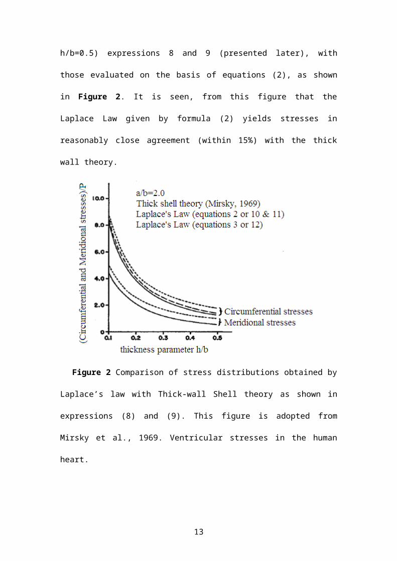
Mirsky (1969) developed expressions for left ventricular stress for a thick prolate
spherioid (which we will present in the subsequent section), using thick shell theory
(Mirsky 1969). He then compared the meridional and circumferential average stresses
in a prolate spheroid obtained from thick shell theory (for h/b=0.5) expressions 8 and
9 (presented later), with those evaluated on the basis of equations (2), as shown in
7
Figure 2. It is seen, from this figure that the Laplace Law given by formula (2) yields
stresses in reasonably close agreement (within 15%) with the thick wall theory.
Figure 2 Comparison of stress distributions obtained by Laplace’s law with
Thick-wall Shell theory as shown in expressions (8) and (9). This figure is adopted
from Mirsky et al., 1969. Ventricular stresses in the human heart.
This Laplace Law can provide a useful and reasonably accurate formula for
calculating average ventricular stresses, which can be employed for determining LV
contractility index (=σ/Pmax), as developed and clinically applied by us (Zhong et al.,
2007 & 2009). The major problem with Laplace Law and thin shell theory is that
there is no variation of stress through the wall. The thick shell theory (and elasticity
theory) provides this variation, which depicts the stress at the endocardial wall
boundary to be maximum. This aspect has a bearing on the reason why myocardial
infarcts are seen to generally occur at the inner wall of the left ventricle.
8
2.2 Left ventricular wall stress based on thick-shell theory In the late 60s, there was a tremendous surge in research work on left ventricular
stresses, inspired by Sandler and Dodge pioneering paper on left ventricular (LV)
stress in Circulation Research in 1963. These works were on the development of LV
stress based on thick shell theory, elasticity theory and large elastic deformation
theory. The thick-wall shell theory enables determination of stress variation across the
LV wall from endocardium to epicardium. It can also include the effects of transverse
normal stress (radial stress) and transverse shear deformation which accompanies
bending stresses. These effects, which are physiologically significant for the left
ventricle, are neglected in the development of Laplace Law. In this section, we will
highlight the two principal works of Wong and Rautharju (1968) and Mirsky (1969).
2.2.1 Wong & Rautharju Model The Wong and Rautharju model analysis (for LV approximated as a thick ellipsoidal
shell) was employed by Hood et al (1969) to determine stress distribution in the LV
wall. Wong and Rautaharju (1968) developed equations which yielded nonlinear
stress distribution across a thick-walled ellipsoidal shell. This made it possible, for the
first time, to compare the mean stresses from thick- and thick-walled ellipsoidal
models. In the Wong and Rautaharju model (1968), the ventricular wall is subjected
to three types of stresses: radial stress (acting perpendicular to the endocardial
surface), longitudinal stress and circumferential stress (acting within the wall at right
angles to each other).
The circumferential stress has been shown to be related to myocardial oxygen
consumption (Graham et al., 1971). Peak systolic circumferential stress has been
adopted as the force factor in the application of the Hill force-velocity concept in
intact man (Gault et al., 1968). Additionally, peak systolic circumferential stress has
been shown to have a bearing on compensatory wall hypertrophy in chronic heart
9

disease (Hood et al., 1969). All these studies employed thin-walled models for
quantifying mean circumferential stress. The validity of thin wall models could only
be resolved after the availability of nonlinear distribution of stress across an
ellipsoidal shell model of LV by Wong and Rautaharju (1968). Although this model is
more sophisticated than that of Sandler and Dodge, it should be emphasized that the
some common same basic assumptions have been made in both models, namely that
wall stress is considered in its passive sense (to be incurred passively form LV
pressure), and the heart myocardial material is an isotropic and homogeneous.
Consequently the factor of fiber orientation and contraction is disregarded. In both
models, other wall forces such as wall shear and bending moments are neglected.
Wong and Rautaharju developed a general equation for stress at any level
from apex to base, whereas Sandler and Dodge solved for stress only at the equator of
the ellipsoidal LV model. Consequently, for the purpose of comparison,
circumferential stress calculations were made only at the equator. Application of
thick-wall theory at the equator permits simplification of the general Wong and
Rautaharju (W&R) equation into an expression using the same terms as that of
equation (2). If is taken to be 0.5, the circumferential stress, at any thickness depth
(T) within the wall in the plane of the equator, is given by (Hood et al., 1969):
(5)
where a=major semiaxis (cm), b=minor semiaxis (cm), P=pressure (dynes/cm2),
and h=wall thickness (cm), Ro= longitudinal radius of curvature at the endocardium =
a2/b, R=Ro+T, n=(2a2+b2)/b2. Hood et al (1969) then employed this W&R equation (5)
to calculate the stress at the endocardium, at the epicardium and at nine evenly spaced
10

points between the endocardium and epicardium. The mean circumferential stress was
then calculated from the following expression:
(6)
which, at the equator becomes:
(7)
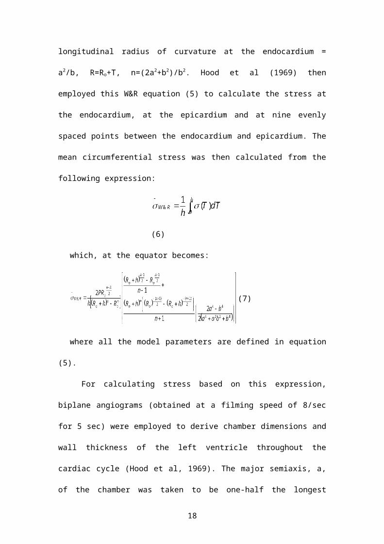
where all the model parameters are defined in equation (5).
For calculating stress based on this expression, biplane angiograms (obtained
at a filming speed of 8/sec for 5 sec) were employed to derive chamber dimensions
and wall thickness of the left ventricle throughout the cardiac cycle (Hood et al,
1969). The major semiaxis, a, of the chamber was taken to be one-half the longest
length measurable within the cavity silhouette on either the antero-posterior or lateral
film. The planimetry silhouette area and measured longest length from each x-ray film
were substituted into the equation for the area of an ellipse, in order to derive the
minor axis. Then the minor axes from each antero-posterior and lateral film pair were
averaged (geometric mean) and divided by two, to give the minor semiaxis (b) of an
idealized prolate ellipsoid. The wall thickness (h) was derived as the average width of
a 4-cm segment of free wall immediately below the equator on each antero-posterior
film. The mean stress based on Sandler & Dodge model and Wong & Rautaharju
model are then compared in terms of the percent error, with the thick-wall stress being
taken as the standard of reference: percent error= .
11

Table 1. Thin-wall versus thick-wall stress analysis (The Table was adopted from Hood et al. Comparison of calculations of left ventricular wall
stress in man from thin-walled and thick-walled ellipsoidal models. Circ Res 1969;XXIV:575-582 )
End-diastole Peak systole End-systoleGroup No
.h/b a/b σS&D σW&R % error h/b a/b σS&D σW&R % error h/b a/b σS&D σW&R % error
Normal left ventricle (EDV=14011)
6 0.350.03
2.10.1
326 295 7.20.8
0.440.03
2.10.1
32624
30424
7.00.8 1.050.09
2.60.1
1230.22
11521
7.80.9
Mitral stenosis (EDV=1218)
9 0.300.02
1.00.1
427 396 7.40.4
0.380.03
2.00.1
35929
33328
8.00.9 0.60.04
2.30.1
19534 18032
8.00.7
Volume overload (EDV=23922)
19 0.310.01
1.80.03
536 485 9.30.5
0.430.03
2.01.0
35419
32818
8.20.5 0.770.09
2.20.03
14720 13018
9.00.6
Pressure overload compensated (EDV=12320)
5 0.430.07
2.00.1
333 313 8.01.0
0.530.05
2.21.0
39343
38541
7.60.7 1.290.28
2.60.1
12238 11336
8.80.7
Pressure or volume overload, decompensated, and primary myocardial disease (EDV=31451)
9 0.350.03
1.70.04
1.70.04
6714
11.20.7
0.380.03
1.70.04
38615
34715
11.60.05
0.520.05
1.80.1
19836 17632
12.30.8
Idiopathic myocardial hypertrophy (EDV=10141)
2 0.820.24
2.00.2
2.00.2
3917
147 1.050.06
2.50.6
17126
1557 11.57.0
2.380.39
2.50.6
6816 5918 18.510.5
12
Selected mean circumferential stress and dimensional data from all subjects
have been summarized in Table 1 (Hood et al., 1969). It can be seen that the degree
of overestimation in terms of percent error usually varies between 5% and 15% in
individual patients and overall averaged about 10% (Table 1).
Comparison of calculated stress at end-diastole shows that the thin-wall
equation overestimates mean thick-wall stress by more than 15%. Furthermore, even
at end-systole when h/b has its maximum value, the percent error between the two
formulae is also around 10%. The Sandler and Dodge formula is simpler and more
convenient to use in clinical application compared to Wong and Rautajarju formula.
However, the Sandler and Dodge formula permits calculation only of mean stress and
only at the equation, whereas, the Wong and Rautaharju analysis permits calculation
of stress at any depth within the wall. It also theoretically allows quantification of
stress at any point on the ventricle, although difficulties in measuring wall thickness
from angiocardiograms in human subjects can limit stress determination to the wall
regions at the equator.
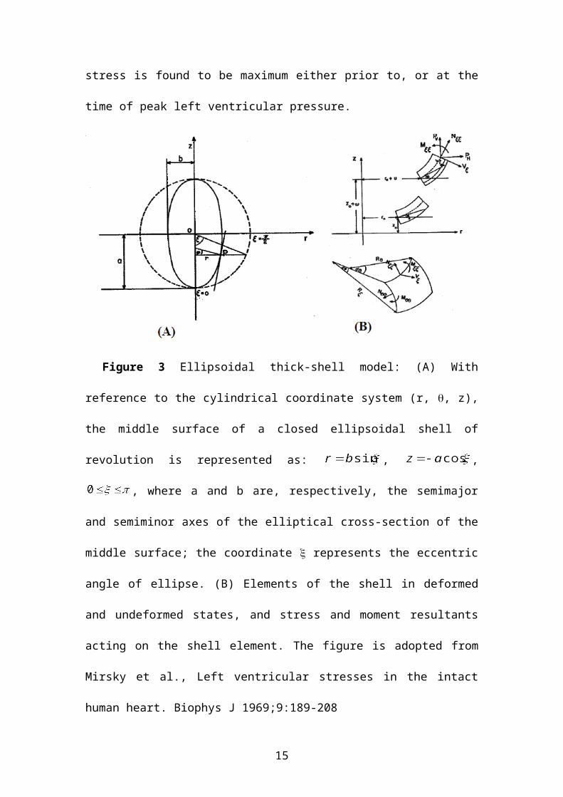
2.2.2 Mirsky thick-shell modelThe Mirsky thick-walled ellipsoidal model, illustrated in Figure 3, includes the effects
of transverse normal stress (radial stress) and transverse shear deformation. The
model presents a system of differential equations for the stress equilibrium in the wall
of the thick-walled prolate spheroid. These equations were derived from the three-
dimensional equations of elasticity, by employing the method of the calculus of
variations. The analysis for the left ventricular stress involves the solution of these
differential equations by numerical integration and asymptotic expansion of
displacement and stress formations. The geometrical data employed in the evaluation
of the stresses was obtained from biplane angiocardiography. The results indicate that
13

maximum stresses occur in the circumferential direction on the endocardial surface at
the equator of the ellipsoid, which we all know now. Also, during a cardiac cycle, this
stress is found to be maximum either prior to, or at the time of peak left ventricular
pressure.
Figure 3 Ellipsoidal thick-shell model: (A) With reference to the cylindrical
coordinate system (r, , z), the middle surface of a closed ellipsoidal shell of
revolution is represented as: , , , where a and b are,
respectively, the semimajor and semiminor axes of the elliptical cross-section of the
middle surface; the coordinate represents the eccentric angle of ellipse. (B)
Elements of the shell in deformed and undeformed states, and stress and moment
resultants acting on the shell element. The figure is adopted from Mirsky et al., Left
ventricular stresses in the intact human heart. Biophys J 1969;9:189-208
For the analysis, the following assumptions were made: (i) the myocardium is
composed of an isotropic and homogeneous elastic material, having the Poisson’s
ratio = 0.5’, (ii) throughout the cardiac cycle, the geometry of the ventricle is
approximated by a prolate spheroid of uniform wall thickness; (iii) instantaneous
14

measurements of geometry and left ventricular pressure were employed in a static
analysis for the evaluation of instantaneous stresses throughout the cardiac cycle; (iv)
ventricular wall stress and deformations are independent of the circumferential
coordinate and are due to the left ventricular pressure only; (v) the effects of
transverse normal stress (radial stress) and transverse shear are included; (vi) the
quasi-static analysis is performed over short intervals of time for which the
deformations are small.
The model coordinate system, the shell element (in deformed and undeformed
states) and the stress and moment resultants are illustrated in Figure 3.
Simplified expressions for the equatorial stresses were obtained as follows:
(8)
where the membrane stresses , , and the bending stresses , are
given by:
(9)
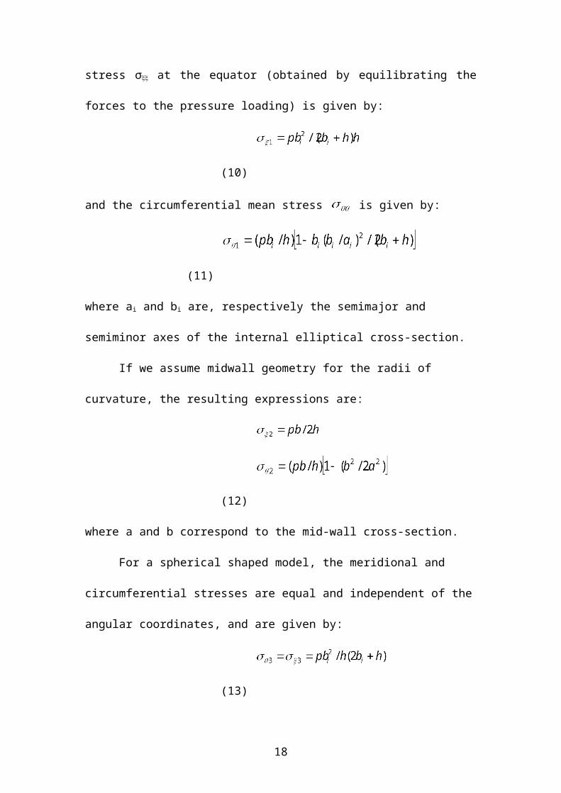
For the purpose of comparison of the stress values obtained by expressions (8
& 9) with those obtained by used of Laplace Law, we will (for the sake of
convenience) again provide the Laplace Law thin shell expressions. For a prolate
15

spheroid, the meridional mean stress σ at the equator (obtained by equilibrating the
forces to the pressure loading) is given by:
(10)
and the circumferential mean stress is given by:
(11)
where ai and bi are, respectively the semimajor and semiminor axes of the internal
elliptical cross-section.
If we assume midwall geometry for the radii of curvature, the resulting
expressions are:
(12)
where a and b correspond to the mid-wall cross-section.
For a spherical shaped model, the meridional and circumferential stresses are
equal and independent of the angular coordinates, and are given by:
(13)
For h<<bi, the stresses at internal wall and midwall are given by:
(14-a)
(14-b)
where bi is the internal radius of the sphere and b is the midwall (or mean) radius.
The exact result for the mean stress is
(15)
where bo is the outer radius of the sphere.
16

For two patients (HW and EWR), the stresses in equations (8 & 9) were
computed from LV biplane angiocardiogram-derived geometry and intra-ventricular
pressure measurements. In Figures 4, the time histories of these two patients HW and
WER are depicted for the maximum (endocardial equatorial) circumferential stress
(σ), along with the circumferential force/unit length (N), in relation to the left
ventricular pressure (LVP). It is seen that the maximum stress occurs either prior to,
or at the time of peak intraventricular pressure. This result demonstrates the
relationship of stress on LV systolic geometry and pressure.
Figure 4. Left ventricular pressure, circumferential stress ( ) and tension/unit
length ( ) versus time for (A) a patient with mild mitral valve insufficiency, (B) a
patient with aortic insufficiently. Note: dynes/cm2=0.1 Pascal. The figure is adopted
from Mirsky et al., Left ventricular stresses in the intact human heart. Biophys J
1969;9:189-208.
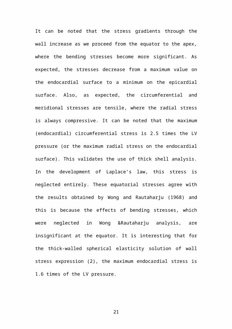
The stress distributions through the wall thickness are depicted in Figure 5 for
three values of (=0, 50 and 90) at the time of maximum stress, for patient WER. It
can be noted that the stress gradients through the wall increase as we proceed from the
equator to the apex, where the bending stresses become more significant. As
17
expected, the stresses decrease from a maximum value on the endocardial surface to a
minimum on the epicardial surface. Also, as expected, the circumferential and
meridional stresses are tensile, where the radial stress is always compressive. It can be
noted that the maximum (endocardial) circumferential stress is 2.5 times the LV
pressure (or the maximum radial stress on the endocardial surface). This validates the
use of thick shell analysis. In the development of Laplace’s law, this stress is
neglected entirely. These equatorial stresses agree with the results obtained by Wong
and Rautaharju (1968) and this is because the effects of bending stresses, which were
neglected in Wong &Rautaharju analysis, are insignificant at the equator. It is
interesting that for the thick-walled spherical elasticity solution of wall stress
expression (2), the maximum endocardial stress is 1.6 times of the LV pressure.
Figure 5: Thick-wall Stress distributions through the wall at three values of for
patient WER. Note: 1 dynes/cm2 = 0.1 Pa. The figure is adopted from Mirsky et al.,
Left ventricular stresses in the intact human heart. Biophys J 1969;9:189-208.
18

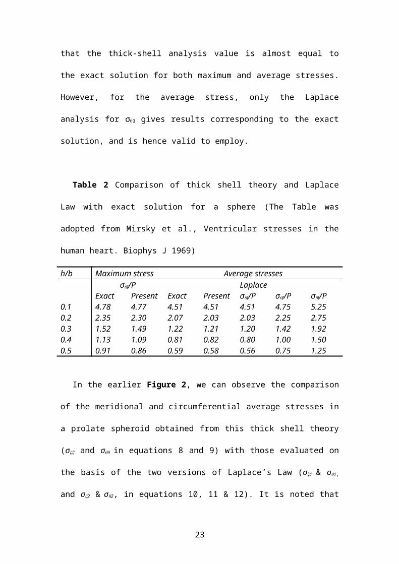
In Table 2, the stresses based on this thick-shell analysis are compared with the
stresses based on (i) the exact solution (15) based on the classical theory of elasticity
for a thick spherical shell (Timoshenko and Goodier, 1951) and (ii) Laplace Law, for
the special case of the sphere. In this table, it is relevant to observe the results for the
realistic case of h/b=0.3. We find that the thick-shell analysis value is almost equal to
the exact solution for both maximum and average stresses. However, for the average
stress, only the Laplace analysis for σ3 gives results corresponding to the exact
solution, and is hence valid to employ.
Table 2 Comparison of thick shell theory and Laplace Law with exact solution for
a sphere (The Table was adopted from Mirsky et al., Ventricular stresses in the human
heart. Biophys J 1969)
h/b Maximum stress Average stressesσI/P Laplace
Exact Present Exact Present σI/P σI/P σI/P0.1 4.78 4.77 4.51 4.51 4.51 4.75 5.250.2 2.35 2.30 2.07 2.03 2.03 2.25 2.750.3 1.52 1.49 1.22 1.21 1.20 1.42 1.920.4 1.13 1.09 0.81 0.82 0.80 1.00 1.500.5 0.91 0.86 0.59 0.58 0.56 0.75 1.25
In the earlier Figure 2, we can observe the comparison of the meridional and
circumferential average stresses in a prolate spheroid obtained from this thick shell
theory (σ and σ in equations 8 and 9) with those evaluated on the basis of the two
versions of Laplace’s Law (σ1 & σ1, and σ2 & σ2, in equations 10, 11 & 12). It is
noted that the modified form of Laplace’ Law based on internal geometry and given
by formulae (10 & 11) are in closer agreement with the thick-wall analysis result. The
meridional stresses are actually identical and the circumferential mean stresses differ
by no more than 15% from the thick-wall theory for relatively thick shells (h/b=0.5).
19

Thus Laplace’s Law formulae, as given by equations (10 & 11), are useful and
reasonably accurate for calculating average (or mean) ventricular wall stress.
The important significance of this thick-shell theory is the variation of
circumferential wall stress through the wall. As seen in Figure 5, the high stress in the
endocardial wall implies that in systole the myocardial oxygen demand is very-high in
the endocardial region. Further the high stress in this region has the effect of
squeezing the coronary vessels in the inner wall region of the LV, which increases the
resistance to coronary flow. This decreases myocardial perfusion in the inner wall
region. Thus, there can arise a situation of oxygen perfusion versus demand
mismatch, resulting in the formation of a myocardial infarct. This is why there is a
preponderance of myocardial infarcts in the inner wall of the LV.
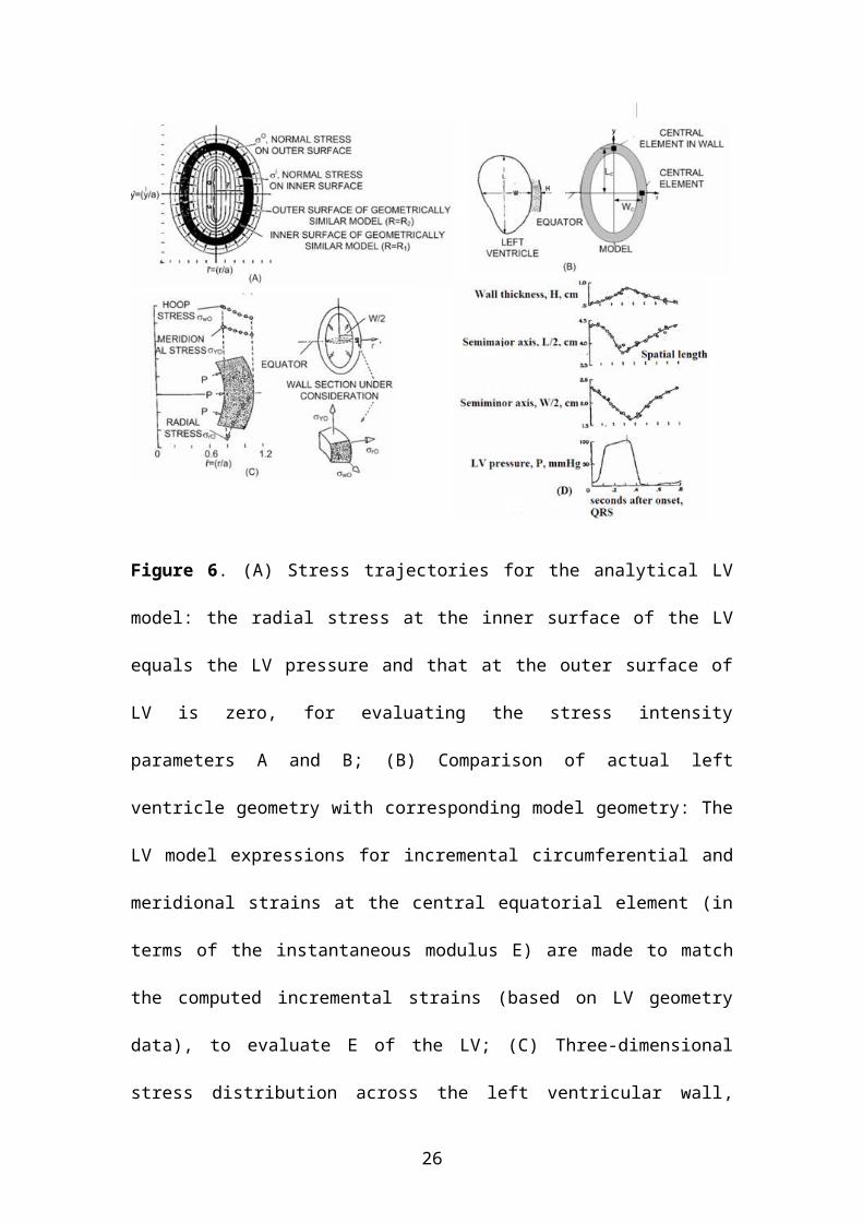
2.3 Left ventricular wall stress formulations from elasticity theoryWe have gone over the 3-dimensional LV models based on thick shell theory of
ellipsoidal shell (Wong et al., 1968; Mirsky 1969), which have certain assumptions
compared to the use of elasticity theory. So we will now study the Ghista and Sandler
3-D elasticity model of the LV. The model simulates the instantaneous 3-D geometry
of the LV by a quasi-ellipsoidal shaped geometry, as depicted in Figure 6 (Ghista et
al., 1969; Ghista et al., 1971). The noteworthy feature of this model is that its shape is
adjustable with the varying shape of the LV, as it becomes more ellipsoidal and
thicker during systole.
20

Figure 6. (A) Stress trajectories for the analytical LV model: the radial stress at the
inner surface of the LV equals the LV pressure and that at the outer surface of LV is
zero, for evaluating the stress intensity parameters A and B; (B) Comparison of actual
left ventricle geometry with corresponding model geometry: The LV model
expressions for incremental circumferential and meridional strains at the central
equatorial element (in terms of the instantaneous modulus E) are made to match the
computed incremental strains (based on LV geometry data), to evaluate E of the LV;
(C) Three-dimensional stress distribution across the left ventricular wall, depicting the
maximum endocardial hoop stress value to be equal to twice the value of chamber
pressure; (D) LV pressure and dimensions during a cardiac cycle, constituting the data
for the model application. These figures are based on the Ghista-Sandler model
(Adapted from Figures of Ghista DN, Sandler H, Med Biol Eng 1975, 13(2):151-160.
21

This model comprises of superposed: (i) Line Dilatation system, over a length “a”
along the longitudinal axis of LV, of amplitude parameter A (Figure 6-A), (ii) and a
hydrostatic stress system, of amplitude parameter B. Incorporating LV catheterization
and cineangiography monitored LV pressure and geometry data in patients, this model
yields (i) the expression for LV wall stresses, (whose variations across the wall are
depicted in Figure 6C), (ii) the principle stress-trajectory surfaces (shown in Figure
6A), having approximately ellipsoidal LV geometry, and (iii) the expressions for the
displacements at these stress-trajectory surfaces. Based on elasticity theory, the model
provides for (i) shear in the ventricular wall, (ii) normal stress in the ventricular wall,
and (iii) variation of stresses across the wall.
For employment of the Ghista-Sandler model, we have first to determine the
shape parameters so that the model’s instantaneous major dimensions (maximum
length L, maximum width W and thickness H) match the corresponding dimensions
of the LV, recorded as shown in Figure 6D.
Shape Parameters of the Model. The analytical model is derived (in
cylindrical coordinates) by superposing a line dilatation force system (obtained by
distributing point dilatations along a portion of length 2a of the Y axis of revolution)
of intensity A, and uniform hydrostatic stress system of intensity B. Stress trajectories
of the combined system are drawn in a plane containing the axis of revolution, with
coordinates , . The two trajectories, whose intercepts’ ratios
, on the axes , equal the ratios of length-to-width of the
inner and outer surfaces of the LV, namely L/W and (L+2H)/(W+2H), are selected to
represent the inner and outer boundaries of the geometrically similar model (See
Figure 6). These intercepts ratios R1 and R2 are referred to as the shape parameters of
the model.
22

Now, to make the geometrically similar model match the actual model in size,
we select the value s of the factor “a” (the size parameter of the model) equal to the
ratio of half-the-width (W/2) of the inner surface LV chamber and the “r” intercept
of the inner boundary of the geometrically similar model. At this stage, the stresses
due to the constituent stress systems of the model are functions of the stress intensity
parameters A and B.
The parameters A and B of the two stress systems are obtained by satisfying
the boundary conditions that (1) the instantaneous change in stress on the inner
surface of the model must equal the instantaneous change in chamber pressure P,
and (2) the stress on the outer surface of the model must be zero. Once the intensity of
parameter A and B are obtained in terms of the data quantities of the LV chamber
pressure and dimensions, the stresses in the model are also expressed completely in
terms of these data quantities.
The stress in the model. The instantaneous stresses in the instantaneous
model of the LV (the instantaneous model simulates the LV at an instant during the
cardiac cycle) are given in dimensionless ( , ) as follows:
23
(16)
where , and .
In the above equations (16), the parameters A and B are given in terms of the
instantaneous values of chamber pressure and dimensions as follow:
(17)
where d1 and d2 are given in terms of the instantaneous width (W) and wall
thickness (H) as follows: ,
We need to note that the stresses given by equation (16) and (17) are due to
the instantaneous changes (P) in pressure P and hence provide instantaneous
changes (σ) in the stresses (equation 16). In order to obtain stress at an instant, we
can sum up the instantaneous stresses (σ) or even put the term P instead of P in
equation (17).
Now, for the central equatorial element shown in Figure 6, the stresses are
given by
24

(18)
where
The Ghista & Sandler (1969) model has added intrinsic features which the
shell models do not have; this is because it is an elasticity model. As can be seen from
Figure 6A, the model resembles a thick-walled ellipsoid of revolution, but allows for
a variation in shape during a cycle as well as for simulation of enlarged LVs of
persons (say, due to regurgitant aortic valve). It can be seen (from the shape of the
stress trajectories) that the model becomes less oval-shaped as the internal cavity gets
bigger as diastolic filling proceeds, and becomes more oval-shaped as its becomes
smaller as during systolic ejection phase. It can also be seen that simulation of
enlarged LV chambers will yield model geometries that are less oval-shaped. This
corresponds to the clinical situation, wherein enlarged LV chambers become less
oval-shaped and more spherically shaped.
This model is hence more representative of the cyclic LV geometry compared
to shell models. This model also then yields a more representative stress distribution
in the LV wall. Further, it being an elasticity model, there is flexibility to make the
model shape even more representative of the LV geometry during the diastole and
systolic phases. For instance, we can shorten the length of the line dilation along the y
axis to make the model more conical in shape. We can also make the model more
innovative by superposing additional stress systems corresponding to a series of
pressurized sphere along the wall, to simulate the pressure of coronary artery vessels
in the wall. We can then study the variation of the size of these coronary artery
25

vessels across the wall thickness, so as to get an idea of how the LV wall stress affects
the wall perfusion.
2.4 Left ventricular wall stress formulations on large deformation theory Thick-wall elasticity and shell models have been developed by Ghista and Sandler
(1969), Wong and Rautaharju (1968) and Mirsky (1969). For thick-wall structures,
the model should include the effects of transverse normal stress (radial stress) and
transverse shear deformation, which always accompanies bending stresses. The
analysis then yields a nonlinear stress distribution through the wall thickness, a result
that can not be predicted by Laplace’s Law.
This far, in the models presented, linear elasticity has been assumed, that is,
deformations of the order 5-10% are assumed to take place. However, during the
contractile and ejection phases, substantial changes in the ventricular dimensions can
occur. For such large deformation, it is more appropriate to apply the large elastic
deformation theory in order to obtain a more accurate description of the stress
distribution.
Mirsky (1973) investigated the specific effect of large deformations on
stresses in the LV, which was approximated by a thick-walled sphere composed of
isotropic, homogeneous, and incompressible material. The stresses at a given pressure
level were calculated from a strain energy density function. Using data from dog
studies (Spotnitz et al; 1966), he evaluated this function at the midwall, based on
strains and cavity and wall volumes at that particular cavity pressure. The nonlinear
relation between stress and strain was assumed to be of exponential form. The major
finding of this study is that inclusion of nonlinear stress-strain properties predicts a
very high stress concentration at the endocardium which is almost 10 times higher
than predicted by linear elasticity theory, as depicted in Figure 7. This stress
26
concentration is noted to increase markedly as the LV cavity pressure is increased,
such as during systole It may well be that such an analysis could provide some insight
into the mechanisms causing ischemia in the endocardial layers of the LV, based on
strain-energy values, evaluated in this region.
Figure 7. The circumferential stress (normalized to the Laplace stress =Pa/2h, based on the classical theory and large deformation theory), is shown plotted as a function of wall thickness. There is a marked difference in the stresses, particularly in the endocardial layer. (The figure is adopted from Mirsky et al., 1973. Review of various theories for the evaluation of left ventricular wall stress. In Cardiac Mechanics, Mirsky I, Ghista DN, Sandler D (eds), pp.381-409)
Another noteworthy contribution to the application of large deformation shell
theory LV is by Chaundhry et al (1995 & 1997), who employed a more realistic
circular-conical shell model (closed at the apical end). Both Mirsky (1973) and
Chaundhry et al used dog studies data of Spontnitz et al (1966) to demonstrate how
LV stresses can be determined.
For the Mirsky LV model, let the spherical coordinate system (R, , ) refer
to the strained state of the model (with its origin at the center of the shell), and (r, ,
27

) coordinate system refer to the unstained state. Denoting the internal and external
radii of the LV shell in the unstrained and strained states by r1, r2 and R1, R2,
respectively, we have the following relations as a based on the incompressibility
condition:
(19)
(20)
The strain energy density function W (the amount of mechanical energy required to
deform a given volume of material) is generally a function of the strain components
rij, namely 11, 22, 33, the radial, circumferential, and meridional strains. However,
for the special case of spherical symmetry with an incompressible material, the strain
energy density function W was taken to be a function of the strain invariant I, given
by:
(21)
so that W is expressed as W=W(I)
The radial and circumferential stresses are given by:
(22-a)
(22-b)
where PH, the hydrostatic pressure, is determined from the equilibrium equation as:
(23)
where and C is a constant of integration to be determined from the
boundary conditions:
on R=R1; on R=R2 (24)
Equations (22, 23 and 24) yield the following relations:
28

(25-a)
where ,
,
,
. (25-b)
The equilibrium condition , given by
(25-b)
serves to determine the deformed radius R1 if the pressure P and the strain energy
density W are known, since R2 can be expressed in terms of R1 via the
incompressibility condition (19).
From the stress expressions (22), is evaluated by employing midwall
values for the stress components ( , ), as obtained from the classical theory of
elasticity for a thick spherical shell (Timoshenko and Goodier, 1951);. These classical
theory stresses are given by:
,
(26)
where V is the left ventricular volume, Vw is the left ventricular wall volume, and the
subscript m denotes the midwall value. Thus, is given by
(27)
29
which can evaluated for each pressure level P if the pressure-volume and pressure-
radii data are known. Now, in order to determine the stress distribution through the
wall of the left ventricle, we require to be expressed as a function of I (which,
as can be seen from equation (20), is a function of the deformed radius R).
For this purpose, for each pressure level, P, the function was
evaluated at the midwall by employing relation (27), and this mid-wall value for
was then plotted against Im, the average of the values for I at the endocardial
and epicardial surface, i.e., . This data were fitted by an exponential
curve: , where A, B, C are constants determined from a nonlinear
regression analysis. These constants were then adjusted until the equilibrium
condition (25-c), , agreed to within 5% of the experimental dog pressure-
radius (P vs R1) data.
Mirsky used pressure-volume data (Table 3) obtained from dog studies by
Spotnitz et al (1966) to obtain:
(28)
With this expression for , the expression (25-c) for K(R2) was computed at 5
mmHg pressure increments over the range 5-30 mmHg, as shown in Table 3. The
calculated K(R2) vs R1 pressure-radius curves matched with the experimental P vs R1
curves.
Table 3 Pressure-volume data and strain-energy density for the left ventricle (The
Table was adopted from Mirsky et al., Ventricular and arterial wall stresses based on
large deformations analysis. Biophys J 1973;13:1141-1159)
P V R1 Rm R2 (әW/әI)m IM
mmHg ml cm mmHg5 31.5 1.96 2.56 3.15 3.73 3.56
30

10 40.0 2.12 2.67 3.22 6.82 3.8615 46.7 2.23 2.74 3.27 9.9 4.120 52.0 2.31 2.80 3.31 13.0 4.2825 56.5 2.38 2.85 3.34 16.1 4.4430 60 2.43 2.90 3.37 19.3 4.56Wall volume Vw=100 ml. At zero pressure, V=12 ml, R1=1.42 cm, R2=2.99cm.
Using this expression, in equation (22), we can determine the stress
distribution through the wall of the LV. Mirsky computed the circumferential and
meridional stresses from equation (22). The earlier Figure 7 depicts LV
circumferential stress ( ) based on both the classical theory (equation 26) and large
deformation theory (equation 22), plotted as a percentage of the wall thickness for a
ventricular pressure P = 20 mmHg. The circumferential stresses are normalized to
(PR1/2h), which is the mean stress as given by the Laplace Law for a sphere (Mirsky
1969). This figure depicts a marked difference in the stress distributions, showing a
10-fold increase in the stress at the endocardial surface over that predicted by the
classical theory.
As we have stated earlier, Mirsky (1973) as well as more recently Chaundhry
et al (1995; 1997) used experimental dog studies data to demonstrate how LV stresses
can be determined by using large deformation theory for thick shells. However, they
did not indicate how this large deformation theory can be applied to human data,
which we will now indicate below.
It can be noticed that for the computation of LV stresses from equation (22),
we need to know the LV undeformed state dimensions r1 and r2 (the inner and outer
dimensions) of the LV at zero internal pressure). It is possible to determine these
dimensions from dog studies for zero internal pressure. However, this can not be done
in human clinical applications. So in human application, in order to determine r1 and
r2, we need to first determine the value of LV volume V0 at zero pressure, from LV
31
geometry and pressure for at least two cardiac cycles. Then from the cyclic pressure-
volume plots, we can determine the volume (V0) at zero pressure by the method
employed by Grossman, Braunwald et al (1977), as illustrated in Figure 8. Herein, it
is seen that V0 can be obtained from two successive values of end-systolic pressure
(Pes) and end-systolic volume (Ves).
As can be seen, the slope of the left ventricular end-systolic pressure volume
relation was relative steep in subjects with normal contractile function (Group A), but
became progressively less steep with greater degrees of impairment in contractile
function. The extrapolated V0 value is small (32 ml/m2) for the group with normal
contractile function, and larger (46 ml/m2 and 10-0 ml/m2) for the groups with
intermediate and poor contractile function, respectively. From the value of V0, we can
determine r1 (the inner radius of the LV model) at zero pressure. The value of r2 (outer
radius of the model) can be thereby obtained from the incompressibility condition of
equation (19).
So, in this way, the Mirsky large-deformation model can be applied to human
data. There is an added application of Figure 8. The parameter m in the equation
Pes=m(Ves-V0) represents the LV systolic elastance Ees, which has an important
bearing on how well an LV matches with the aorta. The ratio of Ees to Ea (aortic
elastance) represents the degree of matching. This LV-aorta matching ratio value is
significantly disturbed for cardiomyopathy LVs. Surgical ventricular restoration
(SVR) is supposed to improve the value of Ees, and the degree to which SVR
improves LV systolic function is based on the improved value of Ees/Ea following
SVR. So in the clinical application, we will see how to noninvasively determine and
clinically apply this LV-aorta matching index (Ees/Ea)
32
Figure 8. Average values for left ventricular end-systolic volume and pressure at
two levels of systolic load are plotted for subjects with normal contractile function
(Group A, ejection fraction >=60%), intermediate function (group B, ejection fraction
= 0.41-0.59), and poor contractile function (group C, ejection fraction <0.40). This
figure is adopted from Grossman et al. Contractile state of the left ventricle in man as
evaluated from end-systolic pressure-volume relations. Circulation 1977;56:845-852.
Now, aside from Mirsky and Chaudhry not applying their work into large-
deformation models to assess in vivo stress, these models also did not incorporate
twisting moments. In fact, the reason why LV is able to generate such a high increase
of pressure (of the order of 50-100mmHg) during ventricular contraction and able to
eject such a high volume of blood into the aorta (of the order of 70-140 ml) is because
of its twisting. This reason for LV twisting when it contracts is because of the
spirally-wound myocardial fibers. It is easy to image how contraction of these
spirally-wound myocardial fibers can cause the LV to twist. Now the LV model to
33
demonstrate these effects of LV twisting, due to contraction of the spirally wound
myocardial fibers, is that of Ghista et al (2009).
2.5 Left ventricular wall stress determination based on precise in-vivo geometry and using finite-element modelling (FEM)
2.5.1 The finite element model trial A more accurate description of the geometry of the heart requires the use of the finite
element model (FEM) for calculation. The FEMs have been developed to incorporate
nonlinear and anisotropic material properties, fiber architecture and nonlinear strains
from animal data. These models were pressurised to simulate the mechanics of the
LV. These LV FEMs provide us useful insights into LV physiology, wall stress
distributions and deformations during diastole and systole.
It is noteworthy that LV models have also been developed to account for the
influence of intramyocardial coronary blood volume upon the stress distribution in the
myocardial tissue (Smith et al., 2000). This is an area that needs extensive work,
because it can provide insights into how wall stress influences intra-myocardial blood
flow and myocardial perfusion, and hence into the formation of myocardial infarcts in
the LV wall.
One of the earliest FEMs of LV was formulated by Gould and Ghista (1972),
who incorporated a realistic longitudinal cross-section of the LV wall into an
axisymmetric FE representation. The effects of the geometric complexity were
examined using rings of isotropic, homogeneous shell elements. The additional
geometric flexibility of this model permitted the wall curvature changes (from
concave to convex inwards) and hence a shift in the location of the peak wall stress
from the endocardium to the epicardium, which idealized geometrical models could
not predict.
34
Janz and Grimm (1972) proposed FE models by incorporating material
anisotropy and heterogeneity, along with more realistic LV geometry. The main
results of this work were that deformations were significantly affected by the degree
of heterogeneity and anisotropy of the myocardium. The isotropic model
underestimated the deformed lumen radius by approximately 8%, and the stress
predicted by the isotropic model differed by factors of two or three from those
predicted by the heterogeneous model. While providing some qualitative insights into
predicted myocardial stress distributions the quantitative accuracy of predicted
stresses was limited by the use of small-strain elasticity theory. Then, Janz et al
(1974) extended their earlier FEM to include large deformation theory.
The earliest 3-D FE model applied to human data was by Ghista and Hamid
(1977). Figure 9 illustrates this model, made up of 20-node, 3-dimensional
isoparametric elements, which precisely simulates the LV geometry. This figure also
displays the stress distributions across the LV wall by both this FE model and that
obtained by Ghista and Sandler elasticity model (Figure 6). It can be seen that the
Ghista and Hamid finite element model yields stress distribution (for radial,
meridonial and hoop stresses) across the wall that very closely match those obtained
analytically by Ghista and Sandler (1969). This gives a measure of confidence into
both the Ghista and Sandler elasticity model and the Ghista & Hamid FE model for
realistic portrayal of the stress distributions in the LV wall.
35
Figure 9. (A) Ghista and Hamid left ventricular finite element model (made up of
20-node, 3-dimensional isoparametric elements), whose irregular shape is developed
from single plane cineangiocardiogram; (B) Comparison of the wall stress
distributions of this finite element model with that obtained from the Ghista and
Sandler elasticity model, indicates close matching of stresses both in magnitude and
distribution across the wall. The figure is adopted from Ghista and Hamid. Finite
element stress analysis of the human left ventricle in Computer Programs in
Biomedicine 1977;7:219-231.
The first non-axisymmetric large deformation FEM of the LV was proposed by
Hunter (1975). This model represented the ventricular myocardium as an
incompressible, transversely isotropic material and incorporated the transmural
distribution of fibre orientations measured by Streeter et al (1973a and 1973b). In this
study, ventricular geometry was measured by mounting silicone filled canine hearts
onto a rig and using a probe to record the radial coordinates of the endocardial and
36

epicardial surfaces at several pre-defined angular and axial locations. Hunter (1975)
used this rig to also measure fibre orientations throughout the ventricular walls, and
this work was subsequently completed by Nielsen et al (1991).
More recent anatomical studies have revealed that the ventricular myocardium
should not be viewed as a uniformly continuous structure, but as a composite of
discrete layers of myocardial muscle fibres bound by endomysial collagen (Le Grice
et al., 1995). It was Nash (1998) who first formulated the anatomically accurate FE
model of ventricular geometry and fibrous structure based on the earlier work of
Nielsen et al (1991). This model incorporated the orthotropic constitutive law, based
on the three-dimensional architecture of myocardium, to account for the nonlinear
material response of the myocardium. The strain results showed good overall
agreement with reported observations from experimental studies of isolated and in-
vivo canine hearts from (Nielsen et al., 1991), which offered credibility to the derived
stress. The computed tensile fiber stress was greatest near the endocardial region of
the apex, while small tensile stresses were obtained for epicardial fibres at the apical
and equatorial regions. Also, smaller fiber stresses were obtained for epicardial
regions near the base.
Later on, other animal FE models were developed from rat (Omens et al.,
1993) and rabbit (Lin et al., 1998; Vetter et al., 2000) were also developed. Figure 10
shows the equibiaxial fiber and cross-fiber stress-strain relations in rabbit, dog and rat.
It showed that rat myocardium is less stiff than the canine myocardium, and that both
materials are stiffer in the fiber direction than in cross-fiber direction, which is to be
expected.
37

Figure 10 Equibiaxial fiber (A) and Cross fiber (B) stress-strain relations from models of the dog (Omens et al., 1993), rat (Omens et al., 1993), rabbit (Lin et al., 1998), and model by Vetter et al., (2000). The material parameters used to model the stress-strain relation in the rat (Omens et al., 1993), dog (Omens et al., 1993) and rabbit (Lin et al., 1998) myocardium and the parameters in Vetter model (2000) are tabulated in (C). The constitutive law, function of the principal strain invariants, is given by:
. The material parameters C, b1, b2, b3 are determined from the myocardial deformation under different loading conditions. This figure is adopted from Vetter et al. Three-dimensional stress and strain in passive rabbit left ventricle: a model study. Annals of Biomedical Engineering 2000;28:781-792.
With the development of modern imaging modalities, some more sophisticated
LV models were developed, which incorporated realistic three-dimensional geometry
38

and fiber architecture, constitutive law for nonlinear anisotropic elastic properties of
myocardium, and boundary conditions of physiologically realistic constrains under
normal or diseased conditions (Guccione et al., 2003; Dang et al., 2005a, 2005b;
Walker et al., 2008). Generally, this kind of finite-element heart modeling includes (1)
in vivo heart geometry from MRI, (2) detailed helical fiber angles from diffusion
tension MRI [Walker et al., 2005b], and (3) myocardial material properties (Moonly
2003). Material properties were generally iteratively determined by comparing the FE
models with experimentally tagged MRI strains measurements.
In fact, in order to develop advanced realistic FE model, connective tissue
[Hooks et al., 2002]; conduction system [Tranum-Jensen et al., 1991] and ventricular
and coronary fluid mechanics [Smith et al., 2000] should also be incorporated. These
physiological processes are interlinked. The electrical activation of the heart initiates
mechanical contraction through intracellular calcium release and is also influenced by
cell stretching in terms of mechano-electric feedback. The supply of oxygen and
metabolic substrates via coronary flow is finely tuned to ATP consumption by cross-
bridges, membrane ion pumps, and other cellular processes. Ventricular fluid inflow
is driven by myocardial diastolic recoil and atrial contraction, and coronary flow is
driven by systolic contraction. The coupling of these processes has been initiated in
the Physiome Project (Hunter et al., 2003; Crampin et al., 2004). A more detailed
account of Physiome Project can be obtained from a recent review by Hunter et al.,
(2003).
2.5.2 Features of constructed finite element models (FEM) Here, we are briefly introducing the framework for the development of advanced FE
models, involving FE geometry determination and computation of stress and strain.
39

Figure 11. (A) Successive series images of the short-axis slices of myocardium cast in dental rubber. After each image was captured, 2-3 mm of the tissue/rubber plug were pressed out of the tube and sliced off exposing the myocardium and rubber of the next image. Successive images are shown in rows stating at the base (upper left) and ending at the apex (lower right); B Segmentation of the ventricular myocardium; (C) The rectangular Cartesian ‘model’ coordinate system is convenient for modeling cardiac geometry. The curvilinear parameters coordinates (1, 2, 3) used in fitting and subsequent analysis, are the local finite element coordinates; (D) Fitted three-dimensional LV geometry with fibre orientation; (E) Schematic of a block cut from a tissue slice, showing the transmural variation in fiber angle and typical images of series cross sections of unstained tissue from the inferior septum with averaging measured fibre angle in the first section is -104 and in the last section is +43; (F) Anterior (left) and posterior lateral (Right) views of the fitted three-dimensional finite element model showing interpolated fiber angles superposed on the epicardial and endocardial surfaces. (the figures are adopted from Vetter FJ, McCulloch AD. Three-dimensional analysis of regional cardiac function: a model of rabbit ventricular anatomy. Progress in Biophysics & Molecular Biolgoy 1998;69:157-183.
40

Finite Element Geometry: To achieve the simulation of cardiac mechanics,
the myocardium geometry and the myocardial fibre orientations are needed as
anatomical inputs into LV models. Figure 11 A-D illustrates the preparation of the 3-
D finite-element model by Vetter et al (1998 & 2000). The excised LV was fixed by
filing its cavity with quick-setting dental rubber, and then its short-axis digital images
were acquired. From these images, the geometrical contours of the rubber-tissue were
segmented (Figure 11A and B) and the geometrical coordinates of the fiducial
markers were recorded by image-processing software (Figure 11C). The LV geometry
was then constructed by fitting a surface through the myocardial contours on tagged
MRI slices, using a prolate spheroidal coordinate system aligned to the central axis of
the LV (Vetter et al., 1998) (Figure 11D).
The transmural variations of the myocardial fibers were measured from the
blocks of tissue cut from the slices (Figure 11E). Most diffusion tensor imaging and
dissection analysis have depicted an elevation angle (angle between the fibre and the
short axis plane) varying from around +70 on the endocardium to around -70 on the
epicardium (Guccione and McCulloch 1991; Hsu and Henriquez 2001), and being
horizontal in the short axis plane at mid-wall. Herein, due to the smoothing in the
discretisation and averaging per tetrahedron, the imaged fiber orientations are seen to
follow a linear variation between +90 to -90 (Figure 11E) (Vetter et al., 1998).
The FE model was then created by placing nodes at equal angular intervals in
the circumferential and longitudinal directions, and by fitting radial coordinates to the
inner and the outer surfaces. The models were subsequently converted into a
rectangular Cartesian coordinate system, with the long axis of the ventricle oriented
along the x-axis and the y-axis directed toward the centre of the right ventricle. The
resulting model consisted of a number finite elements with their geometry
41

interpolated (i) in radial direction using Lagrange basis functions and (ii) in
circumferential and longitudinal direction using cubic Hermite basis functions. The
elements were solid blocks or thin surfaces shells.
The fitted three-dimensional ventricular geometry and fiber angles by Vetter
and McCulloch (1998) are shown in Figure 11F. Over 22500 measurements are
represented by 736 degrees of freedom, with a RMSE of 0.55 mm in the geometric
surface and 19 in the fiber angles. A comparison of the measured fiber angles and
the fitted transmural distribution is shown in Figure 12. The fitted fiber distributions
(by assigning the coordinates) are seen to be in close agreement with the measured
angles and the fitted distribution in the dog (Nielsen et al., 1991).
Figure 12. Measured and fitted fiber angles for the rabbit (crosses and solid lines)
and fitted fiber angles for the dog. Horizontal axes are normalized wall depth (%);
vertical axes are fiber angle (degrees). This figure was adopted from Vetter FJ and
McCulloch AD. Three-dimensional analysis of regional cardiac function: a model of
rabbit ventricular anatomy. Progress in Biophysics & Molecular Biolgoy
1998;69:157-183
42

Computing Stress and Strain using FEA: We have presented the description
of LV FEM construction, based on the work of Vetter and McCullogh (1998). Once
the geometrical construction is done (as per figure 11), the material properties,
boundary, and initial conditions are assigned, and LV pressure simulation can be
carried out. We will now move on to the work of Vetter and McCulogh published in
2000. In this work, the earlier model (Figure 11) was modified to serve as a
computational model for passive LV inflation simulating the control group
experiments of Gallagher et al (1997).
Material Law and Determination of Material Parameters: The
myocardium was modeled (by Vetter and McCulloch, 2000) as a transversely
isotropic, hyperelastic material with an exponential strain energy function (Guccione
et al., 1991; Omens et al., 1993)
,
(29)
where the Lagrangian Green’s strains Ei j are referred to the local fiber coordinate
system consisting of fiber (f), cross fiber (c), and radial (r) coordinate directions. The
material parameters C, b1, b2, and b3 have been described in detail by Guccione et al.
(1991); briefly, the material constant C scales the stress; b1 and b2 scales the material
stiffness in the fiber or cross fiber direction, respectively, and b3 scales the material
rigidity under shear in the fiber-radial and fiber-cross fiber planes.
The LV passive inflation was simulated. The model strains were compared
with experimental measurements, and the material parameters were adjusted to
improve the agreement: b1 and b2 were modified to minimize discrepancies in fiber
and cross fiber strains and b3 was modified according to differences in shear strain.
Vetter and McCulloch computed the root mean squared error (RMSE) of the objective
43
function , where were the model strains and Eij are the epicardial strains
measured by Gallagher et al. (1997) at LV pressures of 5, 10, 15, 20, and 25 mm Hg.
The parameters that minimized the RMSE were accepted as the best estimates of
myocardial material parameters.
Boundary Conditions and Computational Approach: The boundary
conditions were specified by constraining the model displacement degrees-of-
freedom. The model coordinates and their circumferential and transmural derivatives
were constrained at the base on the LV epicardium and RV endocardium. The LV was
passively inflated. The fiber strains and cross-fiber strains distributions are depicted in
Figure 13A.
Figure 13: Part (A) depicts Hammer projection maps of fiber strain (Eff) and cross fiber strain (Ecc) in the LV free wall at 25 mmHg pressure. Contours are drawn at 0.05, 0.10, 0.20 and 0.25 strain levels. Part (B) depicts Cauchy stresses (kPa) resolved in fiber (σff) and cross-fiber (σcc) directions in the LV free wall and apex at 10 mmHg pressure. Contours are drawn at 0, 2, 4, 6, 8 kPa stress levels. These figures are adopted from Vetter FJ and McCulloch AD. Three-dimensional stress and strain in passive rabbit left ventricle: a model study Annals of BioMed Eng 2000;28:781-792.
44

The resulting Cauchy stress distribution is depicted in Figure 13-B. Over the
lateral wall and apex, the Cauchy stress resolved in the fiber direction is seen to be on
an average higher than that in the cross-fiber direction, which can be expected. For the
region shown in Figure 13, the mean fiber stress was 2.913.93 kPa and the mean
cross fiber stress was 1.473.51 kPa. At the midventricle, the fiber stress tended to be
larger than cross fiber stress transmurally. At the epicardium and midwall, the cross-
fiber stress is seen to be more uniform than the fiber stress, while the fiber stress was
greater. The apex and papillary insertions at the subendocardium show the greatest
magnitude and regional variability in both directions, while the negative stresses are
seen to occur predominately at the regions of negative curvature.
2.5.3 Anatomically-accurate bio-elasticity passive-active LV finite element model A representative FE model needs to include the heart’s macroscopic (left and right
ventricular) components and microstructure architecture (of myocardial fibres and
sheets), so as to incorporate the contractile properties of the ventricular myofibers (by
means of the intracellular Ca concentration – fiber tension relationship). This enables
the LV model to simulate (the effect of contractile wave propagation along the
myocardial fibrous network, in terms of) the ventricular apex-to-base twist, which is
the prime factor behind the LV pressure rise during isovolumic contraction to initiate
ejection of blood into the aorta. This is the feature of the Nash model, which was built
up from silicone-filled canine hearts (Nash, 1998).
The model consists of 60 high-order finite-elements and 99 nodes, defined
with respect to a prolate spheroidal coordinate system. The ventricular mechanics
model incorporates the orthotropic pole-zero constitutive law. The nonlinear elastic
properties of passive myocardium were modeled by using 3D orthotropic
45

relationships between the components of the second Piola-Kirchhoff stress tensor and
Green’s strain tensor, to simulate the diastolic phase of the cardiac cycle.
In the model, the contractile forces are generated along the axes of cardiac
fibres and are related to the strain in the fibre. The contractile properties of ventricular
myofibers are approximately by means of a relationship between the fibre extension
ratio, intracellular calcium concentration and active fibre stress. In this way, the LV
model framework incorporated a somewhat realistic model of active myocardial
mechanics.
The ventricular mechanics was analyzed for three of the four main phases of
the heart cycle. The diastolic filling phase inflated the unloaded and residually-
stressed ventricles to physiological end-diastolic LV and RV cavity pressure of 1 kPa
(75 mmHg) and 0.2 kPa (15 mmHg), respectively. During diastolic filling, the LV
volume increased from 32 ml to 52 ml, while the RV volume decreased from 28 ml to
22 ml. This was accompanied by an increase in the LV long axis dimension from 73
mm to 76 mm. The average end-diastolic long-axis rotation (or apex-to-base untwist
angle) was about 5.
Following end-diastole, the level of activation was increased consistently
throughout the myocardium (in terms of Ca concentration) to simulate myofiber
contraction, while the ventricular cavities were held at their end-diastolic volumes. By
the end of this isovolumic contraction phase, the LV and RV cavity pressures
increased to 92 kPa (69 mmHg) and 39 kPa (29 mmHg), respectively, and the LV
long axis dimension decreased to 75 mm.
Ventricular ejection was simulated by decreasing the afterload impedances
imposed on each of the cavities. End-systole occurred when the LV ejection fraction
had reached 44%. At this stage, the LV and RV cavity volumes had decreased to 29
46

ml and 20 ml, respectively, and the LV and RV cavity pressures had decreased to 55
kPa (41 mmHg) and 16 kPa (12 mmHg), respectively. During ejection, the LV long
axis dimension decreased to 69 mm. Ventricular twist was calculated in terms of the
circumferential rotation (relative to the end-diastolic state) with respect to the long
axis coordinate. The rotations were clockwise, when viewed from the apex towards
the base; the mean systolic twist was about 5.
Figure 14A illustrate anterior and posterior views of the computed epicardial
and endocardial end-diastolic fibre stress distributions superimposed on the inflated
ventricles. At end-diastole, due to LV filing pressure, the tensile fibre stress was
greatest near the endocardial region of the apex, while small tensile stresses were
obtained for epicardial fibres at apical and equatorial region. Small compressive fibre
stresses were obtained for the epicardial regions near the base, because of the stiff
constraining effects of the basal ring on the mechanics of the ventricles.
Figure 14 (A) end-diastolic fiber stress distribution superimposed on the inflated ventricles. Fibre stress distributions superimposed on the deformed ventricles at the end of isovolumic contraction (B) and end-ejection (C). Stresses are referred to the unloaded residually stressed state. Lines represent element boundaries of the FE mesh. The figure is adopted from Nash. Mechanics and material properties of the heart using an anatomically accurate mathematical model. 1998.
47

Figures 14B and 14C illustrate anterior and posterior views of the predicted
epicardial and endocardial fibre stress distributions, superimposed on the deformed
ventricles at the end of isovolumic contraction and ejection phases of systole,
respectively. At the end of isovolumic contraction, small compressive stresses were
obtained for the most of the LV endocardium, associated with contraction of the
fibers. At end-systole, small comprehensive stresses were obtained in most of the LV
endocardium.
The ventricular mechanics model’s results of (i) cavity pressure versus volume
relationship, (ii) longitudinal dimension changes, (iii) torsional wall deformations, and
(iv) regional distributions of myocardial strain, during diastolic filling as well as
isovolumic contraction and ejection phases of the cardiac cycle, showed good overall
agreements with observations derived from experimental studies of isolated and in-
vivo canine hearts.
In spite of the physiological useful results of this LV FE model, it can still be
kept in mind that this model has not been applied to human data. Hence, there still
remains the need to demonstrate (i) how the model can be developed form human data
for the important phases of the cardiac cycle (namely, start of diastole, end-diastole,
end isovolumic contraction and end-systole), (ii) how the model deformation can be
monitored (especially LV twist), and (iii) how the LV pressure measurements can be
synchronized with LV geometry and structural measurement. Then only can we
clinically utilize all the features of this model to (i) develop indices for cardiac
contractility, (ii) obtain insight into stress variation across the wall, and (iii) relate LV
fibre structure to LV twist and pressure rise during isovolumic contraction.
48

2.6 Comparison of left ventricular wall stress based on LV models Several geometric models of the LV have been used to estimate cavity volume and
wall volume (Vw) (De Simone et al., 1996; Devereux et al., 1996), the most common
being ellipsoidal and spherical shaped models. With regard to stress calculations,
many formulas have also been proposed.
We will first compare the wall stress distribution values obtained from the
popular thick-wall models of LV. Huisman et al (1980) compared the stresses
predicted from several of the previously presented thick wall models, by using the
same angiographic data obtained in a number of disease states as input to each model
(Wong et al., 1968; Ghista et al., 1969; Mirsky et al., 1969). In each case, the material
was assumed to be isotropic homogeneous, and incompressible. The absolute
magnitude of the calculated wall stress differed, depending on the model used. The
difference in mean stress predicted by a thin sphere compared to a thick-wall sphere
was about 12% at end-diastole and 20% at end-systole.
The stress distribution across the wall for the various models are also
compared (Figure 15). These thick-walled models yield both quantitatively and
qualitatively different results. The circumferential stress gradients predicted by all
models decreased from endocardium to epicardium, but by different amounts.
Without experimental verification, the discrepancy between the thick-walled models
makes it somewhat difficult to compare their accuracy. The longitudinal stress
decreased by 26% from endocardium to epicardium for the Ghista & Sandler model
(1969), but increased by 36% for the Mirsky (1969) model. At the mid- wall, all the
models’ stresses vary by about 16%.
49

Figure 15 Comparison of the stress distribution across the wall for the thick-walled
ellipsoid models demonstrating marked quantitative and qualitative differences
between the models. The WONCO model is a modification of the model of Wong and
Rautaharju (1968) with transverse shear taken into account. (Figure is adopted from
Huisman et al 1980. Comparison of models used to calculate left ventricular wall
force. Med Biol Eng Comput 18:133-144)
Mirsky et al (1990) proposed a simplified analysis for LV stress, based on a
thick spherical shell model, which requires measures or estimates of the cavity
volume V and wall volume Vw. By assuming a spherical geometry for the left
ventricle, the chamber inner radius (Ri), outer radius (Ro), and midwall radius (Rm) are
obtained from relationships.
, , (30)
Then, midwall circumferential stress can be estimated from measured pressure, cavity
volume, wall volume, and Rm according to the following (Mirsky et al., 1990):
50

(31)
Thus, for each value of pressure and volume obtained during the measurement, a
value for and Rm can be obtained from Equations 30 and 31.
We now provide some comparison of stresses obtained from some popular
analytical stress expressions used in cardiology and echocardiography with the
stresses obtained from FE models for (a) spherical, (b) ellipsoidal, (c) anatomic
axisymmetric and (d) anatomic non-axisymmetirc chambers developed by Ingrassia et
al (2008).
The Laplace law for a sphere expresses circumferential stress as a function of
pressure, radius of curvature and thickness, in a simple way as:
(32)
wherein rlong is the longitudinal radius of the curvature and h is the wall thickness
Mirsky (1969) provided the following expression for circumferential stress at
the equator of an ellipsoid (based on Laplace Law):
(33)
where a and b are the midwall semimajor and semiminor axes, respectively. This
formula is a slight modification of the expression given by equation (11).
Janz (1982) proposed a circumferential stress expression, applied to general
axismmetric geometries, as follows:
(34)
wherein rcirc is the circumferential radius of curvature, rlong is the longitudinal radius of
curvature, and is the angle between rlong and the axis of symmetry.
For validation of these expressions, Ingrassia et al (2008) developed a series of
LV FE model chambers (Figure 16 top), to compute and compare the circumferential
stress with the analytical expressions (32-34).
51

The Finite element models developed consisted of 64 incompressible elements
defined in prolate spheroidal coordinates, with hybrid cubic-Hermite linear-Lagrange
tensor product basis functions to yield smooth geometric surfaces and ensure
convergence of regional wall stress. Figure 16 (top) shows examples of the four
levels of geometric complexity: spherical, elliptical, anatomic axisymmtric and
anatomic non-axisymmetric chambers. The anatomic non-axissymmetric shape was
developed from magnetic resonance image slices of an isolated canine LV (Costa et
al., 1996). From this model, the LV anatomic axisymmetric shape was constructed as
a solid of revolution about the long axis, using longitudinal slices through the anterior
papillary muscle. Each LV model shape was scaled to achieve a variety of chamber
sizes and radius-to-thickness ratios, yielding a wider range of stress values for the
analysis. Chamber inflation was simulated by incrementally loading it to cavity
pressure ranging from 1.5 to 3 kPa. Two constitutive laws were used to in the model
to encompass a range of material complexity. The first law concerns the strain energy
potential (W)
(35-a)
expressed as a linear function of the first strain invariant, Ic, with the stiffness
parameter k set to 3 kPa. This represents a hyperelastic, isotropic neo-Hookena
material with a linear stress-strain relationship (Costa et al., 1996). Then, in order to
then model a more realistic complex nonlinear anisotropic relationship, W was
expressed as a Fung-type exponential function of Cauthy-Green strain tensor
components, Eij, referred to fiber coordinates (Guccione et al., 1991),
(35-b)
where ,
52

wherein subscripts R, F and C denote radial, fiber and cross-fiber directions,
respectively. The local muscle fiber angle varied linearly from 83 at the endocardium
to -37 ۫ at the epicardium. The material parameters values (k=0.44 kPa, b1=18.5,
b2=3.58, and b3=1.63) were adopted from Guccione’ work (1991).
The stress values estimated by each of the analytical formulae (32-34) were
compared with the finite element results using linear regression. The resulting values
of R2 and slope were grouped by model geometry and material type, to determine the
range of applicability of each equation. Figure 16B (bottom) summarizes the results
of the regression analysis. All the three analytical expressions for stress yielded
(correlation coefficient) R2 values and slopes (between FEM and analytical equations
32-34) near 1 for the spherical and elliptical geometries (A and B), independent of
material type. However, Laplace’s Law did not work when it was applied to the
anatomically shaped axisymmetric geometry (C), for which the Janz equation was
originally derived. In terms of slope, Janz’s expression (34) was superior to that of
Mirsky’s expression (33), for the anatomic axisymmetric geometry.
However, for the anatomic non-axisymmetric geometry, both Mirsky and Janz
expressions compared favorably in terms of slope, indicating that they give reasonable
approximations of the overall average stress in the FE models. Overall, the results
suggest that the reliability of each of the expressions (32-34) of circumferential wall
stress depends more strongly on the geometry of the chamber than on the complexity
of the material.
53
Figure 16 (Top) Illustration of finite element models for spherical, elliptical,
anatomic axisymmetric, and anatomic non-axisymmetric chambers. Solid surface and
wire mesh represent inner and outer surfaces, respectively. (Bottom) Regression
results R2 values from corrections between stresses obtained from each analytic
equation and the finite element method using (A) linear and (B) exponential material
properties; their corresponding slopes are shown in (C) and (D). The figures are
adopted from Ingrassia CM, Jani SY, Costa KD. 2008. Evaluation of analytic
estimates of ventricular wall stress using the finite element method. Proceedings of
the ASME 2008 SBC, SBC2008-193262)
54

3. DiscussionIn this LV wall stress compendium, we have presented (i) LV thin-wall models for
stress based on Laplace Law, (ii) LV thick-shell ellipsoidal small-strain models, (iii)
LV thick-wall elasticity dynamic-shape model, (iv) LV thick-shell large-deformation
model, and (v) LV FE models. Let us compare the stresses obtained by these models.
Table 1 provides comparison of circumferential wall stress values of subjects
computed by Sandler & Dodge expression (2) for a thin-walled ellipsoidal shell LV
model with the mean stress values computed by Wong & Rautahraju model
expression (7) for a thick-wall ellipsoidal shell. It is seen that the Sandler & Dodge
(1963) expression overestimates the stress by only 10-15% at different values of h/b
at end-diastole, peak systole and end-systole. These stress calculations utilized LV
catheterization and biplane angiogram data.
Table 2 presents comparison of maximum and average stress values computed
by Mirsky thick-shell spherical model expressions (8) and (9) (for b=a) with (i) the
stresses computed from expression (15) based on elasticity theory (in Tinoshenko and
Godier, 1951), and (ii) the stresses computed by Laplace Law expressions (13 and 14)
for various values of h/b. The stresses were computed from monitored biplane
angiography and intraventricular pressure data. It is seen that the discrepancy between
the maximum stress values of thick-shell model and elasticity theory is less than 6%.
There is also close agreement of stresses computed by Laplace Law expression (13)
and that computed by the exact solution (15) based on elasticity theory.
Figure 4 provides the cyclic variation of σ based on Mirsky model (1969),
circumferential with respect to the cyclic variation of LV pressure. In view of σ
being a somewhat complex function of LV pressure and ellipsoidal geometry
parameters, it is interesting to note that σ becomes maximum at the start of the
ejection phase. Mind you, this relationship is still based on the passive stress model.
55

Figure 5 shows the variations across the wall of maximum meridional, circumferential
and radial stresses obtained from Mirsky thick-shell ellipsoidal model. As expected,
the circumferential stresses are maximum on the endocardial surface, and equal to 2.5
times the radial stress on the endocardial surface.
Now, in comparison with the use of fixed-shaped thick-shell models of Wong
& Rantaharju (1968) and Mirsky (1969), Ghista & Sandler (1969) employed elasticity
theory to obtain instantaneous geometries of the LV model corresponding to
monitored angiographic data of LV geometry and stress distributions for monitored
LV chamber pressures. The noteworthy feature of Ghista & Sandler (1969) elasticity
model is that the model shape is more akin to actual LV shape, as the stress
trajectories become less oval shaped for increasing values of r and y. This means that
it is possible to appropriately simulate both more oval-shaped systolic LV geometries
and dilated less oval-shaped LVs as well as dilated LVs due to regurgitant aortic
valve.
Figure 15 provides comparison of the three thick-wall models of Wong &
Rantaharju, Mistry and Ghista & Sandler circumferential and longitudinal stress
variations across the wall. All the models depict this trend of maximum value of
circumferential stress at the endocardial surface decreasing to about 50% of this value
at the epicardial surface. However, because the Ghista & Sandler model has no
restrictive assumptions of shell theory, it can be deemed to be the most representative
of LV shape and stress distribution compared to the other models.
To note the effect of using large-deformation theory, Figure 7 provides
comparison of across-wall variation of LV circumferential stress based on Mirsky
(1973) large-deformation spherical thick-shell model equation (22) and the classical
thick-shell elasticity theory equation (26) (from Timoshenko & Goodier, 1951),
56

normalized with respect to Laplace stress for a sphere (σ=PR/2h). It is seen that the
large-deformation model stress value at the endocardium is over ten times greater than
the stress based on classical theory. These stress computations were based on dog
heart data. For using large deformation theory, it is necessary to know the undeformed
radii (r1 and r2) of the LV at conceptual zero internal pressure. Now, since Mirsky
employed dog pressure-volume data (as depicted in Table 3), it was possible to obtain
these undeformed radii. So to enable application of this large-deformation model to
human data, we have indicated (in figure 8) how we can make use of two successive
values of LV end-systolic pressure-volume values (from two successive cycles) to
extrapolate the values of V0 and thereby obtain the values of r1 and r2 by utilizing the
incompressibility condition.
4. Conclusion and future perspectiveIn this paper, we have comprehensively surveyed left ventricular wall stress models,
based on Laplace Law, thick-shell (small-strain) theory, elasticity theory, thick-shell
large deformation theory, as well as the advanced finite element method (FEM). We
have presented an in-depth analysis of all these models theories, derivations and
results. We have compared the LV wall stress results based on analytical expressions
with those obtained from finite element models. This can now enable the readers to
assess the representativeness of the models, the simplicity vs complexity of the stress
computations, and which model is appropriate for them to use physiologically or
clinically.
There are two comments that we want to make. Firstly, the FE models need to
be based on human data, in order to be assessed to be employable. Then also, the
complexity of their computations needs to be weighed against the relative ease of
employing analytical models. Secondly, these models are all based on simulating LV
57
as passive chamber under pressure, resulting in stresses in the wall. In other words,
the stresses are assumed to result from the pressure in the LV chamber.
Now it is somewhat recognized that LV wall stress can have some association
with cardiac pathophysiology, but that needs unravelling. The pathophysiology is
based on what happens at the sarcomere level. In an infarcted LV, the bioelectrical
wave will skirt the infarcted segments, and also not properly excite the ischemic
segments. As a result, certain sets and segments of myocardial fibers will not be
contracted, and this will reflect on the wall stress distribution. However, all this
requires that we first determine the infarcted segments locations, incorporate them in
the LV FEMs, make the sarcomeres in the infarcted segments not contractile, and
determine the associated wall stress distribution. Then only we will be able to figure
out how wall stresses can reflect pathology based on non-perfused damaged
myocardial segments. This then remains as our future avenue to embark upon.
AcknowledgementsThis work was supported in part by research SERC grants 0921480071 from A*STAR, Singapore, grant NMRC/NIG/1006/2009 from National Medical Research Council, and grant SHF/FG408/2009 from SingHealth Foundation.
Short biographical notes on all contributorsDr. Liang Zhong is a senior research scientist at National Heart Centre Singapore. He obtained his PhD in biomedical engineering at Nanyang Technological University. His research work focuses on cardiac mechanics, involving ventricular diastolic and systolic function, and blood flow vortex in the heart by combining cardiac magnetic resonance (CMR) and computational fluid dynamics (CFD).
Professor Dhanjoo Ghista is a pioneer in biomedical engineering and physics. He has published over 20 books on subjects ranging from cardiovascular physics to physiological mechanics to orthopaedic mechanics. He has developed academic programs at universities in the filed of biomedical engineering, healthcare engineering and management, and sustainable development. He is committed to the advancement of developing countries through educational institutional and sustainable communities development. .
Associate Professor Ru-San Tan is a senior cardiology consultant and director of clinical trial at National Heart Centre Singapore. He is an adjunct associate professor at Duke-NUS University in Singapore. He specializes in non-invasive diagnostic cardiac imaging and has extensive clinical experience in cardiovascular magnetic resonance imaging, echocardiography and nuclear cardiology. His research interests include cardiac imaging in diverse heart diseases, cardiac mechanics, and angiomyogenesis with skeletal myoblasts. References
58

Alter P, Rupp H, Rominger MB, Czerny F, Vollrath A, Klose KJ, Maisch B. 2010. A new method to assess ventricular wall stress in patients with heart failure and its relation to heart rate variability. Int J Cardiol. 139(3):301-303
Arts T, Bovendeerd P, van der Toorn A, Geerts L, Kerckhoffs R, Prinzen F. 2001. Modules in cardiac modeling: mechanics, circulation, and depolariztion wave. In: Functional Imaging and Modeling of the Heart (FIMH’01) No. 2230 in Lecture Notes in Computer Science (LNCS). Pp. 83-90.
Balzer P, Furber A, Delepine S, Rouleau F, Lethimonnier F, Morel O, Tadei A, Jallet P, Geslin P, Le Jeune JJ. 1999. Regional assessment of wall curvature and wall stress in left ventricle with magnetic resonance imaging. Am J Physiol Heart Physiol. 277:H901-H910.
Bestel J, Clement F, Sorine M. 2001. A biomechanical model of muscle contraction. In: Medical Image Computing and Computer-Assisted Intervention (MICCAU’01) Lecture Notes in Computer Science (LNCS) 2208:1159-1161.
Bovendeerd PH, Arts T, Delhaas T, et al. Regional wall mechanics in the ischemic left ventricle: numerical modeling and dog experiments. Am J Physiol. 1996;270:H398–H410.
Chaudhry HR, Bukiet B, Davis AM. 1996. Stresses and strains in the left ventricular wall approximated as a thick conical shell using large deformation theory. J Biol Systems. 4(3):353-372.
Chaudhry HR, Bekiet B, Regan T. 1997. Dynamic stresses and strains in the left ventricular wall based on large deformation theory. Int J Non-linear Mech. 32:621-631.
Costa KD, Holmes JW, McCulloch AD. 2001. Modeling cardiac mechanical properties in three dimensions. Phil Trans R. Soc Lond A. 359:1233-1250
Costa KD et al. 1996a. Three-dimensional FEM for large elastic deformations of ventricular myocardium I: cylindrical and spherical polar coordinates. J Biomech Eng. 118(4):452-463.
Costa KD et al. 1996b. Three-dimensional FEM for large elastic deformations of ventricular myocardium II: prolate spheroidal coordinates. J Biomech Eng. 118(4):464-472.
Crampin EJ, Smith NP, Hunter PJ. 2004. Multi-scale modeling and the IUPS physiome project. J Mol Histol. 35:707-714.
Cupps BP, Moustakidis P, Pomerantz BJ. 2003. Severe aortic insufficiency and normal systolic function: determining regional left ventricular wall stress by finite element analysis. Ann Thorac Surg. 76(3):668-675
Dang AB, Guccione JM, Mishell JM. 2005a. Akinetic myocardial infarcts must contain contracting myocytes: Finite-element model study. Am J Physiol Heart Circ Physiol. 288(4):H1844-H1850.
Dang AB, Guccione JM, Zhang P. 2005b. Effect of ventricular size and patch stiffness in surgical anterior ventricular restoration: A finite element model study. Ann Thorac Surg. 79(1):185-193.
De Simone G, Devereux RB. 2002. Rationale of echocardiographic assessment of left ventricular wall stress and midwall mechanics in hypertensive heart disease. Eur J Echocardiography. 3:192-198.
De Simone G, Devereux RB, Ganau A, Hahn RT, Saba PS, Mureddu GF, Roman MJ, Howard BV. 1996. Estimation of left ventricular chamber and stroke volume by limited M-mode echocardiography and validation by two-dimensional Doppler echocardiography. Am J Cardiol. 78:801-807.
59

Delepine S, Furber AP, Beygui F, Prunier F, Balzer P, Le Jeune JJ, Gesline P. 2003. 3-D MRI assessment of regional left ventricular systolic wall stress in patients with reperfused MI. Am J Physiol Heart Circ Physiol. 284:H1190-H1197.
Devereux RB, Alonso DR, Lutas EM, Gottlieb GJ, Campo E, Saches I, Reichek N. 1996. Echocardiographic assessment of left ventricular hypertrophy: comparison to necropsy findings. Am J Cardiol. 57:450-458.
Di Napoli P, Taccardi AA, Grilli A, Felaco M, Balbone A, Angelucci D. 2003. Left ventricular wall stress as a direct correlate of cardiomyocyte apoptosis in patients with severe dilated cardiomyopathy. Am Heart J. 146:1105-1111.
Douglas P, Reichek N, Plappert P, Muhammad A, Sutton M. 1987. Comparison of echocardiographic methods for assessment of left ventricular shortening and wall stress. J Am Coll Cardiol. 9:945-951.
Feiring A, Rumberger J. 1992. Ultrafast computed tomography analaysis regional radius to wall thickness ratio in normal and volume overloaded human left ventricle. Circulation. 85:1423-1432.
Fujita N, Duerinckx A, Higgins C. 1993. Variation in left ventricular regional wall stress with cine magnetic resonance imaging: normal subjects versus dilated cardiomyopathy. Am Heart J. 125:1337-1345.
Gallagher AM, Omens JH, Chu LL, Covell JW. 1997. Alterations in collagen fibrillar structure and mechanical properties of the healing scar following myocardial infarction. Cardiovasc Pathobiol. 2(1):25-36.
Gault JH, Ross J Jr, Braunwald E. 1968. Contractile state of the left ventricle in man: instantaneous tension-velocity-length relations in patients with and without disease of the left ventricular myocardium. Circ Res. 22:451-463.
Ghista DN, Advani SH, Gaonkar GH, Balachandran K, Brady AJ. 1971. Analysis and physiological monitoring of human left ventricle. J Basic Eng 93:147-161.
Ghista DN, Brady AJ, Ranmakrishnan S. 1973. A three-dimensional analytical (rheological model of the human left ventricle in passive-active states. Biophy J. 13:32-54.
Ghista DN, Hamid S. 1977. Finite element stress analysis of the human left ventricle whose irregular shape is developed from single plane cineangiocardiogram. Comput Programs Biomed. 7(3):219-231.
Ghista DN, Liu L, Chua LP, Zhong L, Tan RS, Tan YS. 2009. Mechanism of left ventricular pressure increase during isovolumic contraction, and determination of its equivalent myocardial fibers orientation. J Mech Med Biol. 9(2):177-198.
Ghista DN, Sandler H. 1969. An analytic elastic-viscoelastic model for the shape and the forces of the left ventricle. J Biomech. 2(1):35-47.
Ghista DN, Sandler H, Vavo WH. 1975. Elastic modulus of the human intact left ventricle determination and physiological interpretation. Med Biol Eng. 13(2):151-160.
Ghista DN, Zhong L, Chua LP, Ng EYK, Lim ST, Chua T. 2005. Systolic modelling of the left ventricle as a mechatronic system: determination of myocardial fiber’s sarcomere contractile characteristics and new performance indices. Mol Cell Biomechan. 2:217-233.
Gould P, Ghista DN, Brombolich L, Mirsky I. 1972. In vivo stresses in the human left ventricular wall: analysis accounting for the irregular 3-dimensional geometry and comparison with idealized geometry analysis. J Biomech. 5(5):521-539.
Graham TP Jr, Jarmakani JM, Canent RV Jr, Anderson PAW. 1971. Evaluation of left ventricular contractile state in children; normal values and observations with a pressure overload. Circulation. 44:1043-1052.
60

Grossman W. 1980. Cardiac hypertrophy: useful adaptation or pathologic process? Am J Med. 69:576-584.
Grossman W, Braunwald E, Mann T, McLaurin L, Green L. 1977. Contractile state of the left ventricle in man as evaluated from end-systolic pressure-volume relations. Circulation. 56:845-852
Guccione JM, Costa KD, McCulloch AD. 1995. Finite element stress analysis of left ventricular mechanics in the beating dog heart. J Biomech. 28:1167–1177.
Guccoine JM, McCulloch AD, Waldman LK. 1991. Passive material properties of the intact ventricular myocardium determined from a cylindrical model. ASME J Biomech Eng. 113:42-55.
Guccione JM, Salahieh A, Moonly SM. 2003. Myosplint decrease wall stress without depressing function in the failing heart: A finite element model study. Ann Thorac Surg. 76(4):1171-1180.
Hayashida WT, Kumada R, Nohara H, Tanio M, Kambayashi N, Ishikawa Y, Nakamura Y, Himura Y, Kawai C. 1990. Left ventricular wall stress in dilated cardiomyopathy. Circulation. 82:2075-2083.
Hefner LL, Sheffield LT, Cobbs GC, Klip W. 1962. Relation between mural force and pressure in the left ventricle of the dog. Circ Res. 11:654-663.
Hill AV. 1950. Mechanics of the contractile element of muscle. Nature 165:415.Hood WP, Thomson WJ, Rachley CE, Rolett EL. 1969. Comparison of calculation of
left ventricular wall stress in man from thin-walled and thick-walled ellipsoidal models. Circ Res. 24:575-585.
Hooks DA, Tomlinson KA, marsden SG, LeGrice IJ, Smaill BH. 2002. Cardiac microstructure: implication for electrical propagation and defibrillation in the heart. Circ Res. 91:331-338.
Hsu E, Henriquez C. 2001. Myocardial fiber orientation mapping using reduced encoding diffusion tensor imaging. J Cardiovas Magn Reson. 3:325-333;
Huisman RM, Elzinga G, Westerhof N, Sipkema P. 1980. Measurement of left ventricular wall stress. Cardiovasc Res. 14:142-153.
Humphrey JD, Strumpf RK, Yin FCP. Determination of a constitutive relation for passive myocardium: I Parameter estimation. J Biomech Eng. 1990;112:340-346.
Hunter 1975. Finite element analysis of cardiac muscle mechanics, PhD thesis, University of Oxford.
Hunter P. 1997. Myocardial constitutive laws for continuum mechanics models of the heart. In Molecular and subcellular cardiology: effect of structure and function. Sideman S and Beyar R (eds), Plenum Press, pp. 303-318.
Hunter P, Pullan A, Smail B. 2003. Modeling total heart function. Ann Rev Biomed Eng. 5:147-177.
Huxley AF. 1957. Muscle structure and theories of contraction. Prog Biophys Chem. 7:255
Huyghe JM, van Campen DH, Arts T, Heethaar RM. 1991. The constitutive behavior of passive heart muscle tissue: A quasi-linear visco-elastic formulation. J Biomech. 24:841-849;
Ingrassia CM, Jani SY, Costa KD. 2008. Evaluation of analytic estimates of ventricular wall stress using the finite element method. Proceedings of the ASME 2008 Summer Bioengineering Conference. SBC2008-193262.
Jan KM. 1985. Distribution of myocardial stress and its influence on coronary blood flow. J Biomech. 18:815-820.
Janz R. 1982. Estimation of local myocardial stress. Am J Physiol Heart Circ Physiol. 242:H875-H881
61

Janz RF, Grimm AF. 1972. Finite-element model for the mechanical behaviour of the left ventricle: prediction of deformation in the potassium-arrested rat heart. Circ Res. 30:244-252.
Laplace PS. 1806. Theorie de I’action capillarie. In Traite de mecanique celeste, Supplement au livre X. Paris, Coarcien.
Le Grice IJ, Smaill BH, Chai LZ, Edgar SG, Gavin JB, Hunter PJ. 1995. Laminar structure of the heart: ventricular myocyte arrangement and connective tissue architecture in the dog. Am J Physiol. 269(38):H571-H582.
Lin DHS, Yin YCP. 1998. A multiaxial constitutive law for mammalian left ventricular myocardium steady-state barium contracture or tetanus. J Biomech Eng. 120(4):504-517.
Mann DL. 2004. Basic mechanisms of left ventricular remodeling: the contribution of wall stress. J Cardiac Fail. 10(6):S202-S206.
Mirsky I. 1969. Left ventricular stresses in the intact human heart. Biophys J. 9:189-208.
Mirsky I. 1974. Review of various theories for the evaluation of left ventricular wall stress. In Cardiac Mechanics. Mirsky I, Ghista DN, Sandler H (eds). John Wiley & Sons INC., New York pp.381-409.
Mirsky I. 1973. Ventricular and arterial wall stresses based on large deformations analyses, Biophy J. 13:1141-1159.
Mirsky I, Pasipoularides A. 1990. Clinical assessment of diastolic function. Prog Cardiovasc Dis. 32:291-318.
Misra JC, Singh SI. 1985. Distribution of stresses in the left ventricular wall of the intact heart. Bull Math Biol. 47:53-70.
Moonly S. 2003. Experimental and computational analysis of left ventricular aneurysm mechanics. University of California, San Francisco with University of California; Berkeley, San Francisco, CA.
Moriarty TF. 1980. The law of Laplace, its limitations as a relation for diastolic pressure, volume or wall stress of the left ventricle. Circ Res. 46:321-331.
Nash M. 1998. Mechanics and material properties of the heart using an anatomically accurate mathematical model. PhD thesis, The University of Auckland, New Zealand.
Nielsen PM, Hunter PJ, Smail BH. 1991. Biaxial testing of membrane biomaterials: testing equipment and procedures. J Biomech Eng. 113:295-300.
Nielsen PMF, LeGrice IJ, Smail BH, Hunter PJ. 1991. A mathematical model of the geometry and fibrous structure of the heart. Am J Physiol. 260:H1365-H1378.
Omens JH, MacKenna DA, McCulloch AD. 1993. Measurement of strain and analysis of stress in resting rat left ventricular myocardium. J Biomech. 26(6):665-676.
Pouleur H, Rousseau M, Van Eyll C, Charlier A. 1984. Assessment of regional left ventricular relaxation in patients with coronary artery disease: importance of geometric factors and changes in wall thickness. Circulation. 69:696-702.
Prunier F, Brette S, Delepine S, Geslin P, Le Jeune JJ, Furber AP. 2008. Three-dimensional MRI assessment of regional wall stress after acute myocardial infarction predicts postdischarge cardiac events. J Magn Reson Imaging. 27(3):516-521.
Rohde LE, Aikawa M, Cheng GC, Sukhova G, Solomon SD, Libby P, Pfeffer J, Pfeffer MA, Lee RT. 1999. Echocardiography-derived left ventricular end-systolic regional wall stress and matrix remodeling after experimental myocardial infarction. J Am Coll Cardiol. 33:835-842.
62

Sandler H, Dodge HT. 1963. Left ventricular tension and stress in man. Circulation. 13:91-101.
Schwitter J, Eberli FR, Ritter M, Turina M, Krayenbuehl HP. 1992. Myocardial oxygen consumption in aortic valve disease with and without left ventricular dysfunction. Br Heart J. 18:815-820.
Smith NP, Mulquiney PJ, Nash MP, Bradley CP, Nickerson DP, Hunter PJ. 2002. Mathematical modeling of the heart: cell to organ. Chaos Solitons and Fractals. 13:1613-1621.
Smith NP, Pullan AJ, Hunter PJ. 2000. Generation of an anatomically based geometric coronary model. Ann Biomed Eng 28;14-25
Solomon SD, Martini M, Rosario L. 1998. Regional wall stress following myocardial infarction estimated by echocardiography-based structural analysis. J Am Soc Echocardiog. 32:1819-1824.
Spontnitz HM, Sonnenclick EH, Spiro D. 1966. Relation of ultrastructure to function in intact heart: sarcomere structure relative to pressure-volume curves of intact left ventricles of dog and cat. Circulation Res 18:49-59
Streeter DD, Hanna WT. 1973a. Engineering mechanics for successive states in canine left ventricular myocardium: I Cavity and wall geometry. Circ Res 33:639-655.
Streeter DD, Hanna WT. 1973b. Engineering mechanics for successive states in canine left ventricular myocardium: II Fibre angle and sarcomere length. Circ Res. 33:656-664.
Timoshenko S, Goodier JN. 1951. Theory of elasticity. McGraw-Hill Book Co., New York.
Tranum-Jensen J, Wilde AAM, Vermeulen JT, Janse MJ. 1991. Morphology of electrophysiologically identified junctions between Purkinje fibres and ventricular muscle in rabbit and pig hearts. Circ Res. 69;429-437.
Turcani M, Rupp H. 1997. Etomoxir improves left ventricular performance of pressure-overloaded rat heart. Circulation. 96:3681-3686.
Vetter FJ, McCulloch AD. 1998. Three-dimensional analysis of regional cardiac anatomy. Prog Biophy Mol Biol. 69:157-184.
Vetter FJ, McCulloch AD. 2000. Three-dimensional stress and strain in passive rabbit left ventricle: a model study. Ann Biomed Eng. 28(7):781-792.
Wall ST, Walker JC, Healy KE, Ratcliffe MB, Guccione JM. 2006. Theoretical impact of the injection of material into the myocardium. Circulation. 114:2627-2635.
Walker JC, Ratcliffer MB, Zhang P, Wallace AW, Fata B, Hsu EW, Saloner D, Guccione JM. 2005. MRI-based finite-element analysis of left ventricular aneurysm. Am J Physiol Heart Circ Physiol. 289(2):H692-H700.
Walker JC, Ratcliffe MB, Zhang P, Wallace AW, Hsu EW, Saloner DA, Guccione JM. 2008. Magnetic resonance imaging-based finite element stress analysis after linear repair of left ventricular aneurysm. J Thorac Cardiovasc Surg. 135(5):1094-1102.
Wong AYK, Rautarharju PM. 1968. Stress distribution within the left ventricular wall approximated as a thick ellipsoidal shell. Am Heart J. 75:649-662.
Yin FC. 1981. Ventricular wall stress. Circ Res. 49:829-842.Yin FCP, Strumpf RK, Chew PH, Zeger SL. 1987. Quantification of the mechanical
properties of noncontracting canine myocardium under simultaneous biaxial loading. J Biomech. 20:577-589;
63

Zhong L, Sola S, Tan RS, Le TT, Ghista DN, Kurra V, Navia JL, Kassab G. 2009a. Effects of surgical ventricular restoration on LV contractility assessed by a novel contractility index in patients with ischemic cardiomyopathy. Am J Cardiol. 103(5):674-679.
Zhong L, SU Y, Yeo SY, Tan RS, Ghista DN, Kassab G. 2009b. Left ventricular regional wall curvedness and wall stress in patients with ischemic dilated cardiomyopathy. Am J Physiol Heart Circ Physiol. 296:H573-H584.
Zhong L, Tan RS, Ghista DN, Ng EYK, Chua LP, Kassab GS. 2007. Validation of a novel noninvasive cardiac index of left ventricular contractility in patients. Am J Physiol Heart Circ Physiol. 292(6):H2764-H2772.
64


