

Newnes MechanicalEngineer’s Pocket Book
H6508-Prelims.qxd 9/23/05 11:43 AM Page i

This page intentionally left blank

Newnes MechanicalEngineer’s Pocket Book
Third edition
Roger L. Timings
AMSTERDAM • BOSTON • HEIDELBERG • LONDON • NEW YORK
OXFORD • PARIS • SAN DIEGO • SAN FRANCISCO • SINGAPORE
• SYDNEY • TOKYO
Newnes is an imprint of Elsevier
H6508-Prelims.qxd 9/23/05 11:43 AM Page iii

NewnesAn imprint of ElsevierLinacre House, Jordan Hill, Oxford OX2 8DP30 Corporate Drive, Burlington, MA 01803
First published 1990Reprinted 1992, 1993, 1995 (twice)Second edition 1997Reprinted 2001Reprinted 2002Third edition 2006
Copyright © 1990, Roger Timings and Tony May. All rights reservedCopyright © 1997, 2006 Roger Timings. All rights reserved
The right of Roger Timings to be identified as the author of this work has been asserted in accordance with the Copyright, Designs and Patents Act 1988
No part of this publication may be reproduced in any material form (including photocopying or storing in any medium by electronic means and whether or not transiently or incidentally to some other use of this publication) without the written permission of the copyright holder except in accordance with the provisions of the Copyright, Designs and Patents Act 1988 or under the terms of a licence issued by the Copyright Licensing Agency Ltd, 90 Tottenham Court Road, London, England W1T 4LP.Applications for the copyright holder’s written permission to reproduce any part of this publication should be addressed to the publisher
Permissions may be sought directly from Elsevier’s Science & Technology Rights Department in Oxford, UK: phone: (�44) 1865 843830, fax: (�44) 1865 853333, e-mail: [email protected]. You may also complete your request on-line via the Elsevier homepage(http://www.elsevier.com), by selecting ‘Customer Support’ and then ‘Obtaining Permissions’
British Library Cataloguing in Publication DataA catalogue record for this book is available from the British Library
Library of Congress Cataloguing in Publication DataA catalogue record for this book is available from the Library of Congress
ISBN-13: 978-0-7506-6508-7ISBN-10: 0-7506-6508-4
Typeset by Charon Tec Pvt. Ltd, Chennai, IndiaPrinted and bound in Great Britain
For information on all Newnes publicationsvisit our website at http://books.elsevier.com
H6508-Prelims.qxd 9/23/05 11:43 AM Page iv

Contents
Foreword xix
Preface xxi
Acknowledgements xxvii
1 Engineering Mathematics 11.1 The Greek alphabet 11.2 Mathematical symbols 11.3 Units: SI 21.3.1 Basic and supplementary units 21.3.2 Derived units 21.3.3 Units: not SI 31.3.4 Notes on writing symbols 41.3.5 Decimal multiples of units 41.4 Conversion factors for units 41.4.1 FPS to SI units 51.4.2 SI to FPS units 51.5 Preferred numbers 61.6 Mensuration 61.6.1 Plane figures 61.6.2 Solid objects 91.7 Powers, roots and reciprocals 131.8 Progressions 161.8.1 Arithmetic progressions 161.8.2 Geometric progressions 161.8.3 Harmonic progressions 171.9 Trigonometric formulae 171.9.1 Basic definitions 171.9.2 Identities 181.9.3 Compound and double angle formulae 181.9.4 ‘Product and sum’ formulae 181.9.5 Triangle formulae 181.10 Circles: some definitions and properties 191.10.1 Circles: areas and circumferences 201.11 Quadratic equations 211.12 Natural logarithms 211.13 Statistics: an introduction 211.13.1 Basic concepts 211.13.2 Probability 22
H6508-Prelims.qxd 9/23/05 11:43 AM Page v

1.13.3 Binomial distribution 221.13.4 Poisson distribution 231.13.5 Normal distribution 231.14 Differential calculus (Derivatives) 241.15 Integral calculus (Standard forms) 261.15.1 Integration by parts 281.15.2 Definite integrals 281.16 Binomial theorem 281.17 Maclaurin’s theorem 281.18 Taylor’s theorem 28
2 Engineering Statics 292.1 Engineering statics 292.2 Mass, force and weight 292.2.1 Mass 292.2.2 Force 292.2.3 Vectors 302.2.4 Weight 312.2.5 Mass per unit volume (density) 312.2.6 Weight per unit volume 312.2.7 Relative density 322.2.8 Pressure (fluids) 332.3 Vector diagrams of forces: graphical solution 342.3.1 Resultant forces 342.3.2 Parallelogram of forces 342.3.3 Equilibrant forces 362.3.4 Resolution of forces 362.3.5 Three forces in equilibrium (triangle of forces) 372.3.6 Polygon of forces: Bow’s notation 372.3.7 Non-concurrent coplanar forces (funicular
link polygon) 392.4 Moments of forces, centre of gravity and
centroids of areas 412.4.1 Moments of forces 412.4.2 Principle of moments (related terminology) 422.4.3 Principle of moments 432.4.4 Equilibrium 452.5 Orders of levers 472.5.1 First-order levers 472.5.2 Second-order levers 482.5.3 Third-order levers 492.6 Centre of gravity, centroids of areas and equilibrium 492.6.1 Centre of gravity (solid objects) 492.6.2 Centre of gravity of non-uniform and composite solids 492.6.3 Centre of gravity (lamina) 51
vi Contents
H6508-Prelims.qxd 9/23/05 11:43 AM Page vi
2.6.4 Centroids of areas 522.6.5 Equilibrium 532.7 Friction 542.7.1 Lubrication 552.7.2 Laws of friction 552.7.3 Coefficient of friction 552.7.4 Angle of friction 572.7.5 Friction on an inclined plane 572.7.6 Angle of repose 582.8 Stress and strain 592.8.1 Direct stress 592.8.2 Shear stress 602.8.3 Direct strain 612.8.4 Shear strain 612.8.5 Modulus of elasticity (Hooke’s law) 612.8.6 Modulus of rigidity 622.8.7 Torsional stress 632.8.8 Hoop stress in thin cylindrical shells 642.8.9 Longitudinal stress in thin cylindrical shells 652.9 Beams 662.9.1 Shearing force 662.9.2 Bending moment 672.9.3 Shearing force and bending moment diagrams 682.9.4 Beams (cantilever) 732.10 Stress, strain and deflections in beams 742.10.1 Bending stress and neutral axis 742.11 Frameworks 782.11.1 Method of sections 792.12 Hydrostatic pressure 832.12.1 Thrust on a submerged surface 842.12.2 Pascal’s law 85
3 Engineering Dynamics 873.1 Engineering dynamics 873.2 Work 873.3 Energy 883.3.1 Conservation of energy 883.4 Power 893.5 Efficiency 893.6 Velocity and acceleration 893.6.1 Speed 903.6.2 Velocity 903.6.3 Acceleration 903.6.4 Equations relating to velocity and acceleration 90
Contents vii
H6508-Prelims.qxd 9/23/05 11:43 AM Page vii

3.6.5 Momentum 903.6.6 Newton’s laws of motion 903.6.7 Gravity 913.6.8 Conservation of momentum 923.6.9 Impact of a fluid jet on a fixed body 923.6.10 Inertia 933.6.11 Resisted motion 933.7 Angular motion 963.7.1 The radian 963.7.2 Angular displacement 973.7.3 Angular velocity 973.7.4 The relationship between angular and linear velocity 973.7.5 Angular acceleration 983.7.6 Torque 983.7.7 Work done by a torque 1003.7.8 Centripetal acceleration and centripetal force 1013.7.9 Centrifugal force 1023.8 Balancing rotating masses 1033.8.1 Balancing co-planar masses (static balance) 1033.8.2 Balancing co-planar masses (dynamic balance) 1033.9 Relative velocities 1063.9.1 Relative velocities (unconnected bodies) 1063.9.2 Relative velocities (connected bodies) 1083.10 Kinematics 1093.10.1 Ballistics 1093.11 Kinetics 1103.11.1 Universal gravitation 1103.11.2 Linear translation 1113.11.3 Translation in a curved path 1113.11.4 Conic pendulum 1113.11.5 Rotation of a body about a fixed axis 1133.11.6 Radius of gyration 1143.11.7 Centre of percussion 1143.11.8 Angular momentum 1143.12 Simple harmonic motion 1163.12.1 Simple pendulum 1173.12.2 Natural vibration 1183.13 Fluid dynamics 1193.13.1 Rate of flow 1193.13.2 Continuity of flow 1203.13.3 Energy of a fluid in motion (Bernoulli’s equation) 1203.13.4 Flow through orifices 1213.13.5 Viscosity 1213.13.6 Poiseulle’s formula 1223.13.7 Stoke’s formula 122
viii Contents
H6508-Prelims.qxd 9/23/05 11:43 AM Page viii
4 Fastenings 1234.1 Screwed fastenings 1234.1.1 Drawing proportions 1234.1.2 Alternative screw heads 1254.1.3 Alternative screw points 1254.1.4 Hexagon socket cap head screw 1264.1.5 Application of screwed fasteners 1264.1.6 Acme thread form 1274.1.7 Square thread form 1274.1.8 Buttress thread form 1274.1.9 V-thread form 1284.1.10 Basic Whitworth (55°) thread form: parallel threads 1284.1.11 ISO metric and ISO 60° unified thread forms 1294.1.12 Introduction to screwed fasteners 1294.1.13 BS EN ISO 4014: 2001 Hexagon head bolts –
product grades A and B 1324.1.14 BS EN ISO 4016: 2001 Hexagon head bolts –
product grade C 1394.1.15 BS EN ISO 4017: 2001 Hexagon head screws –
product grades A and B 1454.1.16 BS EN ISO 4018: 2001 Hexagon head screws –
product grade C 1514.1.17 BS EN ISO 4032: 2001 Hexagon nuts style 1 –
product grades A and B 1584.1.18 BS EN ISO 4033: 2001 Hexagon nuts style 2 –
product grades A and B 1624.1.19 BS EN ISO 4034: 2001 Hexagon nuts style 1 –
product grade C 1654.1.20 BS EN ISO 4035: 2001 Hexagon thin nuts
(chamfered) – product grades A and B 1674.1.21 BS EN ISO 4036: 2001 Hexagon thin nuts
(unchamfered) – product grade B 1694.1.22 BS EN ISO 8765: 2001 Hexagon head bolts with
metric fine pitch threads – product grades A and B 1704.1.23 BS EN ISO 8676: 2001 Hexagon head screws with
metric fine pitch threads – product grades A and B 1774.1.24 BS EN ISO 8673: 2001 Hexagon nuts style 1 with
metric fine pitch threads – product grades A and B 1844.1.25 BS EN ISO 8674: 2001 Hexagon nuts style 2 with
metric fine pitch threads – product grades A and B 1874.1.26 BS EN ISO 8675: 2001 Hexagon thin nuts with
metric fine pitch threads – product grades A and B 1904.1.27 BS 7764: 1994 Hexagon slotted nuts and castle nuts 1924.1.28 BS EN ISO 898-1: 1999 Mechanical properties of
fasteners: bolts, screws and studs 196
Contents ix
H6508-Prelims.qxd 9/23/05 11:43 AM Page ix
4.1.29 BS EN ISO 898-1: 1999 Marking 2054.1.30 BS EN 20898-2: 1994 Mechanical properties of
fasteners: nuts with specified proof load values – coarse thread 209
4.1.31 BS EN ISO 898-6: 1996 Mechanical properties of fasteners: nuts with specified proof load values –fine pitch thread 217
4.1.32 BS EN 20898-7: 1995 Mechanical properties of fasteners: torsional test and minimum torques for bolts and screws with nominal diameters 1–10 mm 221
4.1.33 BS EN ISO 4762: 2004 Metric hexagon sockethead screws 222
4.1.34 BS EN ISO 10642: 2004 Hexagon socket countersunk head screws 230
4.1.35 BS4827 ISO metric screw threads, miniature series 2354.1.36 BS3643-1/2 ISO metric screw threads:
constant pitch series 2364.1.37 BS EN ISO 228-1: 2003 Pipe threads where
pressure-tight joints are not made on the threads 2404.1.38 ISO Pipe threads, tapered: basic sizes 2464.1.39 British Standard Whitworth (BSW) bolts and nuts 2504.1.40 British Standard Fine (BSF) bolts and nuts 2514.1.41 ISO unified precision internal screw threads:
coarse series (UNC) 2524.1.42 ISO unified precision external screw threads:
coarse series (UNC) 2544.1.43 ISO unified precision internal screw threads:
fine series (UNF) 2564.1.44 ISO unified precision external screw threads:
fine series (UNF) 2574.1.45 British Association thread form 2584.1.46 BA internal and external screw threads 2594.1.47 BA threads: tapping and clearance drills 2604.1.48 ISO metric tapping and clearance drills,
coarse thread series 2604.1.49 ISO metric tapping and clearance drills,
fine thread series 2614.1.50 ISO unified tapping and clearance drills,
coarse thread series 2614.1.51 ISO unified tapping and clearance drills,
fine thread series 2624.1.52 ISO metric tapping and clearance drills,
miniature series 2624.1.53 BSW threads, tapping and clearance drills 2634.1.54 BSF threads, tapping and clearance drills 263
x Contents
H6508-Prelims.qxd 9/23/05 11:43 AM Page x
4.1.55 Plain washers, bright: metric series 2634.1.56 Plain washers, black: metric series 2644.1.57 Friction locking devices 2654.1.58 Positive locking devices 2674.1.59 Single coil square section spring washers:
metric series, type A 2694.1.60 Single coil rectangular section spring washers:
metric series, types B and BP 2704.1.61 Double coil rectangular section spring washers:
metric series, type D 2724.1.62 Toothed lock washers, metric 2734.1.63 Serrated lock washers, metric 2764.1.64 ISO metric crinkle washers: general engineering 2794.1.65 T-slot profiles 2804.1.66 Dimensions of T-bolts and T-nuts 2824.1.67 Dimensions of tenons for T-slots 2864.2 Riveted joints 2884.2.1 Typical rivet heads and shanks 2884.2.2 Typical riveted lap joints 2894.2.3 Typical riveted butt joints 2904.2.4 Proportions for hole diameter and rivet length 2914.2.5 Cold forged snap head rivets 2924.2.6 Hot forged snap head rivets 2934.2.7 Tentative range of nominal lengths associated with
shank diameters 2944.2.8 POP® rivets 2954.2.9 POP® range guide 2964.2.10 Good fastening practice 2974.2.11 Selection of POP® (or blind) rivets 2974.2.12 Design guidelines 2984.2.13 POP® ‘F’ series 3024.2.14 Open type aluminium 3.5% magnesium alloy 3054.2.15 Open type carbon steel 3134.2.16 Closed end type aluminium 5% magnesium alloy 3184.2.17 Blind rivet nuts 3204.2.18 POP® Nut Threaded Inserts: application 3214.2.19 POP® Nut Threaded Inserts: installation 3224.2.20 POP® Nut: Steel 3244.3 Self-secured joints 3284.3.1 Self-secured joints 3284.3.2 Allowances for self-secured joints 3294.4 Miscellaneous fasteners 3314.4.1 Taper pins, unhardened 3314.4.2 Circlips, external: metric series 3354.4.3 Circlips, internal: metric series 338
Contents xi
H6508-Prelims.qxd 9/23/05 11:43 AM Page xi
4.5 Adhesive bonding of metals 3414.5.1 Anaerobic adhesives 3414.5.2 Adhesives cured by ultraviolet light 3414.5.3 Adhesives cured by anionic reaction (cyanoacrylates) 3444.5.4 Adhesives cured with activator systems
(modified acrylics) 3444.5.5 Adhesives cured by ambient moisture 3454.5.6 Epoxy adhesives 3454.5.7 Redux process 3494.5.8 Bonded joints 349
5 Power Transmission 3515.1 Power transmission: gear drives 3515.1.1 Some typical gear drives 3515.1.2 Simple spur gear trains 3545.1.3 Compound spur gear train 3555.1.4 The involute curve 3565.1.5 Basic gear tooth geometry 3575.1.6 Gear tooth pitch 3615.1.7 Gear tooth height 3625.1.8 Standard gear tooth elements (in.) 3635.1.9 Fine pitch gear tooth elements (in.) 3645.1.10 Standard stub gear tooth elements (in.) 3655.1.11 Standard gear tooth elements (metric) 3665.1.12 Letter symbols for gear dimensions and calculations 3685.1.13 Basic spur gear calculations 3695.1.14 Basic helical gear equations 3705.1.15 Miscellaneous gear equations 3705.1.16 Straight bevel gear nomenclature 3715.1.17 Worm and worm wheel nomenclature 3725.2 Power transmission: belt drives 3735.2.1 Simple flat-belt drives 3735.2.2 Compound flat-belt drives 3745.2.3 Typical belt tensioning devices 3755.2.4 Typical V-belt and synchronous-belt drive applications 3765.2.5 ULTRAFLEX® narrow-section wrapped V-belts 3805.2.6 FO®-Z heavy-duty cogged raw edge V-belts 3825.2.7 MULTIFLEX® classical-section wrapped V-belts 3845.2.8 MULTIBELT banded V-belts 3865.2.9 V-belt pulleys complying with BS 3790 and
DIN standard 2211 for FO®-Z and ULTRAFLEX® belts.Rz xx refers to surface roughness 388
5.2.10 V-belt pulleys complying with DIN standard 2217Part 1 for FO®-Z and MULTIFLEX® belts 390
xii Contents
H6508-Prelims.qxd 9/23/05 11:43 AM Page xii

5.2.11 Deep-groove pulleys 3925.2.12 Synchronous belt drives: introduction 3945.2.13 Synchronous belt drives: belt types and sizes 3985.2.14 Synchronous belt drives: pulleys 4045.2.15 SYNCHROBELT® HTD 4105.2.16 SYNCHROBELT® HTD synchronous (toothed) belts:
tooth profiles 4115.2.17 Synchronous (toothed) belts: length measurement 4145.2.18 SYNCHROBELT® HTD toothed pulleys: preferred sizes 4155.3 Power transmission: chain drives 4195.3.1 Chain performance 4195.3.2 Wear factors 4215.3.3 Chain types 4225.3.4 International Standards 4235.3.5 Standards reference guide 4245.3.6 Advantages of chain drives 4245.3.7 Chain selection 4265.3.8 Sprocket and chain compatibility 4285.3.9 Drive layout 4315.3.10 Selection method 4335.3.11 Rating chart construction 4405.3.12 European chain rating chart 4415.3.13 ANSI rating chart 4425.3.14 Chain suspension force 4435.3.15 Lubrication 4435.3.16 Lubricating methods 4445.3.17 Lifting applications 4465.3.18 ANSI Xtra range 4485.3.19 Influences on chain life 4485.3.20 Chain extension 4505.3.21 Matching of chain 4515.3.22 To measure chain wear 4525.3.23 Repair and replacement 4535.3.24 Chain adjustment 4545.3.25 Design ideas 4555.3.26 Table of PCD factors 4575.3.27 Simple point to point drives: Example one 4585.3.28 Simple point to point drives: Example two 4605.3.29 Simple point to point drives: Example three 4625.3.30 Safety warnings 4665.4 Power transmission: shafts 4675.4.1 Square and rectangular parallel keys, metric series 4675.4.2 Dimensions and tolerances for square and
rectangular parallel keys 4695.4.3 Square and rectangular taper keys, metric series 471
Contents xiii
H6508-Prelims.qxd 9/23/05 11:43 AM Page xiii

5.4.4 Dimensions and tolerances for square and rectangular taper keys 473
5.4.5 Woodruff keys and keyways, metric series 4755.4.6 Dimensions and tolerances for Woodruff keys 4775.4.7 Shaft ends types: general relationships 4795.4.8 Dimensions and tolerances of cylindrical shaft ends,
long and short series 4805.4.9 Dimensions of conical shaft ends with parallel keys,
long series 4825.4.10 Dimensions of conical shaft ends with diameters
above 220 mm with the keyway parallel to the shaft surface, long series 484
5.4.11 Dimensions of conical shaft ends with parallel keys, short series 485
5.4.12 Transmissible torque values 4875.4.13 Straight-sided splines for cylindrical shafts, metric 4885.5 Tapers 4915.5.1 Self-holding Morse and metric 5% tapers 4915.5.2 Tapers for spindle noses 4995.5.3 Tapers for tool shanks 5055.5.4 Tool shank collars 5075.5.5 Bridgeport R8 taper 5085.6 Fluid power transmission systems 5095.6.1 A typical pneumatic system 5105.6.2 A typical hydraulic system 5115.6.3 Air compressor types 5135.6.4 Hydraulic pumps 5155.6.5 Actuators (linear) 5215.6.6 Actuators (rotary) 5235.6.7 Hybrid actuator systems 5245.6.8 Symbols for fluid power systems 5245.6.9 Fluid power transmission design data
(general formulae) 5275.6.10 Fluid power transmission design data
(hydraulic cylinders) 5295.6.11 Fluid power transmission design data
(hydraulic pipes and hoses) 5315.6.12 Fluid power transmission design data
(hydraulic fluids, seals and contamination control) 5325.6.13 Fluid power transmission design data
(hydraulic accumulators) 5345.6.14 Fluid power transmission design data
(hydraulic cooling and heating) 5365.6.15 Fluid power transmission design data
(pneumatic valve flow) 537
xiv Contents
H6508-Prelims.qxd 9/23/05 11:43 AM Page xiv

5.6.16 Fluid power transmission design data (pneumatic cylinders) 538
5.6.17 Fluid power transmission design data (seals, filtration and lubrication) 540
5.6.18 Fluid power transmission design data (air compressors) 541
5.6.19 Fluid power transmission design data (tables and conversion factors in pneumatics) 542
5.6.20 Guideline documents 546
6 Engineering Materials 5486.1 Mechanical properties 5486.1.1 Tensile strength 5486.1.2 Compressive strength 5486.1.3 Shear strength 5486.1.4 Toughness: impact resistance 5496.1.5 Elasticity 5496.1.6 Plasticity 5496.1.7 Ductility 5506.1.8 Malleability 5506.1.9 Hardness 5516.1.10 Tensile test 5516.1.11 Interpretation of a tensile test: material showing
a yield point 5526.1.12 Interpretation of a tensile test: proof stress 5536.1.13 Interpretation of a tensile test: secant modulus 5546.1.14 Impact testing for toughness: Izod test 5556.1.15 Impact testing for toughness: Charpy test 5556.1.16 Interpretation of impact test results 5566.1.17 Brinell hardness test 5566.1.18 Vickers hardness test 5576.1.19 Rockwell hardness test 5576.1.20 Rockwell superficial hardness test 5586.1.21 Comparative hardness scales 5596.2 Ferrous metals and alloys 5606.2.1 Ferrous metals: plain carbon steels 5606.2.2 Effect of carbon content on the composition,
properties and uses of plain carbon steels 5616.2.3 Ferrous metals: alloying elements 5616.2.4 British standards relating to ferrous metals 5636.2.5 Some typical steels and their applications 5656.2.6 Some typical tool steels 5726.2.7 Flake (grey), cast irons 5746.2.8 BS EN 1561: 1997 Grey cast irons 575
Contents xv
H6508-Prelims.qxd 9/23/05 11:43 AM Page xv
6.2.9 Malleable cast irons 5796.2.10 Spheroidal graphite cast irons 5826.2.11 Alloy cast irons 5846.2.12 Composition, properties and uses of
some typical cast irons 5856.3 Non-ferrous metals and alloys 5866.3.1 Non-ferrous metals and alloys – introduction 5866.3.2 High copper content alloys 5866.3.3 Wrought copper and copper alloys: condition code 5876.3.4 British Standards relating copper and copper alloys 5876.3.5 Copper and copper alloy rods and sections 5886.3.6 Wrought copper and copper alloys 5906.3.7 Wrought copper and copper alloys 5956.3.8 Copper sheet, strip and foil 5976.3.9 Brass sheet, strip and foil: binary alloys of
copper and zinc 5996.3.10 Brass sheet, strip and foil: special alloys and
leaded brasses 6036.3.11 Phosphor bronze sheet, strip and foil 6056.3.12 Aluminium bronze alloys – introduction 6076.3.13 Aluminium bronze sheet, strip and foil 6086.3.14 Copper–nickel (cupro–nickel) sheet, strip and foil 6096.3.15 Nickel–silver sheet, strip and foil 6116.3.16(a) Miscellaneous wrought copper alloys 6136.3.16(b) Miscellaneous wrought copper alloys 6156.3.17(a) Copper alloys for casting: group A 6176.3.17(b) Further copper alloys for casting: group A 6186.3.18(a) Copper alloys for casting: group B 6206.3.18(b) Further copper alloys for casting: group B 6226.3.19(a) Copper alloys for casting: group C 6246.3.19(b) Further copper alloys for casting: group C 6266.3.20 Copper alloys for casting: typical properties and
hardness values 6286.3.21 Aluminium and aluminium alloys 6326.3.22 British Standards 6326.3.23 Unalloyed aluminium plate, sheet and strip 6346.3.24 Aluminium alloy plate, sheet and strip:
non-heat-treatable 6366.3.25 Aluminium alloy plate, sheet and strip: heat-treatable 6396.3.26 Aluminium and aluminium alloy bars, extruded
tube and sections for general engineering: non-heat-treatable 642
6.3.27 Aluminium alloy bars, extruded tube and sections for general engineering: heat-treatable 644
6.3.28 Aluminium alloy castings, group A: general purpose 647
xvi Contents
H6508-Prelims.qxd 9/23/05 11:43 AM Page xvi

6.3.29 Aluminium alloy castings, group B: special purpose 6486.3.30 Aluminium alloy castings, group C: special purpose
and of limited application 6496.3.31 Aluminium alloy castings: mechanical properties 6506.3.32 BS EN 29453: 1993 6516.3.33 Typical uses of soft solders 6536.3.34 Silver soldering (hard soldering) 6536.3.35 Group AG: silver brazing filler metals 6546.4 Metallic material sizes 6556.4.1 Metallic material sizes: introduction to BS 6722: 1986 6556.4.2 Recommended diameters of wires, metric 6566.4.3 Recommended dimensions for bar and flat products 6576.4.4 Recommended widths and lengths of flat products 6576.4.5 Mass of metric round and square bars 6586.4.6 Hexagon bar sizes for screwed fasteners, metric 6606.4.7 Gauge sizes and equivalents 6616.5 Polymeric (plastic) materials 6626.5.1 Polymeric (plastic) materials – introduction 6626.5.2 Some important thermosetting polymers 6646.5.3 Some important thermoplastic polymers 665
7 Linear and Geometric Tolerancing of Dimensions 666
7.1 Linear tolerancing 6667.1.1 Limits and fits 6667.1.2 Classes of fit 6677.1.3 Accuracy 6677.2 Standard systems of limits and fits (introduction) 6687.2.1 Application of tables of limits and fits 6687.2.2 Selection of tolerance grades 6707.3 Geometric tolerancing 6727.3.1 Geometrical tolerance (principles) 6747.3.2 Tolerance frame 6777.3.3 Geometrical tolerance 6777.3.4 Tolerance zone 6787.3.5 Geometrical reference frame 6787.3.6 Applications of geometrical tolerances 6797.4 Virtual size 6817.5 The economics of geometrical tolerancing 682
8 Computer-Aided Engineering 6848.1 Computer numerical control 6848.1.1 Typical applications of computer numerical control 684
Contents xvii
H6508-Prelims.qxd 9/23/05 11:43 AM Page xvii

8.1.2 Advantages and limitations of CNC 6848.1.3 Axes of control for machine tools 6858.1.4 Control systems 6878.1.5 Program terminology and format 6888.1.6 Word (or letter) address format 6888.1.7 Coded information 6898.1.8 Data input 6928.1.9 Tool length offsets: milling 6928.1.10 Cutter diameter compensation: milling 6928.1.11 Programming techniques: milling and drilling 6958.1.12 Programming example: milling 6968.1.13 Tool offsets: lathe 6988.1.14 Tool nose radius compensation: lathe 6998.1.15 Programming techniques: lathe 7008.1.16 Programming example: lathe 7028.1.17 Glossary of terms 7048.2 Computer-aided design 7068.2.1 An introduction to computer-aided design 7068.2.2 CAD system hardware 7088.2.3 CAD system software 7108.2.4 Computer-aided design and manufacture 7118.2.5 Advantages and limitations of CAD 7128.3 Industrial robots 7128.3.1 An introduction to robotics 7128.3.2 Robot control 7138.3.3 Robot arm geometry 713
Appendix 1 BSI Standards: Sales Order and Enquiry Contacts 718Appendix 2 Library Sets of British Standards in the UK 722Appendix 3 Contributing Companies 726Appendix 4 Useful References 728
Index 729
xviii Contents
H6508-Prelims.qxd 9/23/05 11:43 AM Page xviii

Foreword
It is now 14 years since the first edition of the Mechanical Engineer’sPocket Book was published in its present format. Although a second edi-tion was published some 7 years ago to accommodate many updates inthe British Standards incorporated in the text, no changes were made tothe structure of the book.
During the 14 years since the first edition of the Mechanical Engineer’sPocket Book was published, the British Engineering Industry has under-gone many changes, with the emphasis moving from manufacture todesign and development. At the same time manufacturing has beenlargely out-sourced to East Europe, Asia and the Far East in order toreduce operating costs in an increasingly competitive global market.
Therefore, before embarking on this third edition, the Publishers and theAuthor have undertaken an extensive market research exercise. The mainoutcomes from this research have indicated that:
● The demand has changed from an engineering manufacturing drivenpocket book to an engineering design driven pocket book.
● More information was requested on such topic areas as roller chaindrives, pneumatic systems and hydraulic systems in the section onpower transmission.
● More information was requested on selected topic areas concerningengineering statics, dynamics and mathematics.
● Topic areas that have fallen out of favour are those related to cuttingtools. Cutting tool data is considered less important now that the empha-sis has move from manufacture to design. Further, cutting tool data isnow widely available on the web sites of cutting tool manufacturers. Aselection of useful web sites are included in Appendix 4.
Roger L. Timings (2005)
H6508-Prelims.qxd 9/23/05 11:43 AM Page xix

This page intentionally left blank

Preface
As stated in the foreword, this new edition of the Mechanical Engineer’sPocket Book reflects the changing nature of the Engineering Industry in theUK and changes in the related technology. Many of the British Standards(BS) quoted in the previous editions have been amended or withdrawn andreplaced by BS EN and BS EN ISO standards. The British Standards catalogueis no longer available in hard copy but is published on a CD.
Definitions of entries
Catalogue entries are coded as in the example shown below. The variouselements are labelled A–J. The key explains each element. Not all the elem-ents will appear in every Standard.
�A �B �C �D
BS 1361: 1971 (1986) � IEC 269-1Specification for cartridge fuses for a.c. circuits in domestic and similar premises.Requirements, ratings and tests for fuse links, fuse bases andcarriers. Dimensions and time/current zones for fuse links.Type 1-rate 240 V and 5–45 A for replacement by domesticconsumers; Type II-rated 415 V and 60, 80 or 100 A for use bythe supply authority in the incoming unit of domestic andsimilar premises.
AMD 4171, January 1983 (Gr 0) R 00000821AMD 4795, January 1985 (Gr 2) R 00000833 �EAMD 6692, January 1991 (FOC) 00000845
�J A5, 44 pages GR7 PEL/3200000818
�I �H �G �F
H6508-Prelims.qxd 9/23/05 11:43 AM Page xxi
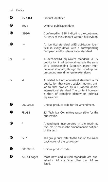
�A BS 1361 Product identifier.
�B 1971 Original publication date.
�C (1986) Confirmed in 1986, indicating the continuingcurrency of the standard without full revision.
�D � An identical standard: a BSI publication iden-tical in every detail with a correspondingEuropean and/or international standard.
or � A (technically) equivalent standard: a BSIpublication in all technical respects the sameas a corresponding European and/or inter-national standard, though the wording andpresenting may differ quite extensively.
or � A related but not equivalent standard: a BSIpublication that covers subject matters simi-lar to that covered by a European and/orinternational standard. The content howeveris short of complete identity or technicalequivalence.
�E 00000833 Unique product code for the amendment.
�F PEL/32 BSI Technical Committee responsible for thispublication.
�G R Amendment incorporated in the reprintedtext. No ‘R’ means the amendment is not partof the text.
�H GR7 The group price: refer to the flap on the insideback cover of the catalogue.
�I 00000818 Unique product code.
�J A5, 44 pages Most new and revised standards are pub-lished in A4 size. Sizes other than A4 arelisted.
xxii Preface
H6508-Prelims.qxd 9/23/05 11:43 AM Page xxii

Amendments
All separate amendments to the date of despatch are included with anymain publication ordered. Prices are available on application. The amend-ment is then incorporated within the next reprint of the publication and thetext carries a statement drawing attention to this, and includes an indica-tion in the margin at the appropriate places on the amended pages.
Review
The policy of the BSI is for every standard to be reviewed by the technicalcommittee responsible not more than 5 years after publication, in order toestablish whether it is still current and, if it is not, to identify and set inhand appropriate action. Circumstances may lead to an earlier review.
When reviewing a standard a committee has four options available:
● Withdrawal: indicating that the standard is no longer current.● Declaration of Obscelence: indicating by amendment that the standard
is not recommended for use in new equipment, but needs to beretained for the servicing of existing equipment that is expected to havea long service life.
● Revision: involving the procedure for new projects.● Confirmation: indicating the continuing currency of the standard with-
out full revision. Following confirmation of a publication, stock of copiesare overstamped with the month and year of confirmation.
The latest issue of standards should always be used in new productdesigns and equipments. However many products are still being manu-factured to obsolescent and obsolete standards to satisfy a still buoyantdemand. This is not only for maintenance purposes but also for currentmanufacture where market forces have not yet demanded an update indesign. This is particularly true of screwed fasteners. For this reason theexisting screw thread tables from the previous editions have beenretained and stand alongside the new BE EN ISO requirements.
The new standards are generally more detailed and prescriptive thanthere predecessors, therefore there is only room to include the essentialinformation tables in this Pocket Book as a guide. Where further informa-tion is required the full standard should always be consulted and a list oflibraries holding up-to-date sets of standards is included in an appendix atthe end of this book. The standards quoted in the Pocket Book are up-to-date at the time of publication but, in view of the BSI’s policy of regularreviews, some may become subject to revision within the life of this book.
Preface xxiii
H6508-Prelims.qxd 9/23/05 11:43 AM Page xxiii

For this reason the validity of the standards quoted should always be veri-fied. The BSI helpline should be consulted.
This Pocket Book has been prepared as an aid to mechanical engineersengaged in the design, development and manufacture of engineeringproducts and equipment. It is also a useful source book for others whorequire a quick, day-to-day reference of engineering information. For easyreference this book is divided into 8 main sections, namely:
1. Mathematics2. Engineering statics3. Engineering dynamics4. Fasteners5. Power transmission6. Materials7. Linear and geometrical tolerancing8. Computer aided engineering.
Within these main sections the material has been assembled in a logicalsequence for easy reference and numbered accordingly. This enables thereader to be lead directly to the item required by means of a comprehen-sive list contents and the inclusion of a comprehensive alphabetical index.
This Pocket Book is not a text book but a compilation of useful informa-tion. Therefore in the sections concerned with mathematics, statics anddynamics worked examples are only included where anomalies might oth-erwise occur. The author is indebted to the British Standards Institutionand to all the industrial and commercial companies in the UK and abroadwho have co-operated in providing up-to-date data in so many technicalareas. Unfortunately, limitations of space have allowed only abstracts to beincluded from amongst the wealth of material provided. Therefore thereader is strongly recommended to consult the complete standards, indus-trial manuals, design manuals or catalogues after an initial perusal of thetables of data found in this book. To this end, an appendix is provided withthe names and addresses of the contributors to this book. They all haveuseful web sites where additional information may be found.
The section on computer-aided manufacture has been deleted from thisedition as it was too brief to be of much use and could not be expandedwith in the page count available. Specialist texts are available on applica-tion from the publishers of this Pocket Book on such topic areas as:
● Computer numerical control● Computer-aided drawing and design● Industrial robots● Flexible manufacturing systems
xxiv Preface
H6508-Prelims.qxd 9/23/05 11:43 AM Page xxiv

● Programmable logic controllers● Manufacturing management● Project management.
Within the constraints of commercial viability, it is the continuing inten-tion of the author and publisher to update this book from time to time.Therefore, the author would appreciate (via the publishers) suggestionsfrom the users of this book for additions and/or deletions to be taken intoaccount when producing new editions.
Roger L. Timings (2005)
Preface xxv
H6508-Prelims.qxd 9/23/05 11:43 AM Page xxv

This page intentionally left blank

Acknowledgements
We would like to thank all the companies who have kindly given permis-sion for their copyright material to be used in this edition:
British Fluid Power Association (BFPA) (Sections 5.6.9–5.6.18, 5.6.20).ContiTech United Kingdom Ltd. (Sections 5.2.4–5.2.18).David Brown Engineering Ltd. (Section 5.1.1).Henkel Loctite Adhesives Ltd. (Sections 4.5.1–4.5.9).IMI Norgren Ltd. (Section 5.6.19).National Broach & Machine Co. (Sections 5.1.4–5.1.17).Renold plc. (Sections 5.3–5.4, 5.3.10–5.3.13, 5.3.16, 5.3.18–5.3.19,
5.3.21–5.3.22, 5.3.27–5.3.30).Emhart Teknologies (Tucker Fasteners Ltd.) (Sections 4.2.8–4.2.18).Butterworth Heinemann for allowing us to reproduce material from
Higgins, R. A., Properties of Materials in Sections 6.2.2, and 6.2.3.Butterworth Heinemann for allowing us to reproduce material from Parr,
Andrew, Hydraulics and Pneumatics in Sections 5.6.1–5.6.4.Newnes for allowing us to reproduce material from Stacey, Chris, Practical
Pneumatics in Section 5.6.3.Pearson Education Ltd., for allowing us to reproduce material from
Timings, R. L., Materials Technology volumes 1 and 2 in Sections6.1.1–6.1.21 and 7.1–7.5.
Extracts from British Standards are reproduced with permission of BSI.Complete copies of these documents can be obtained by post from BSISales, Linford Wood, Milton Keynes, Bucks., MK14 6LE.
Further information concerning the above companies can be found in theAppendix 3 at the end of this Pocket Book.
H6508-Prelims.qxd 9/23/05 11:43 AM Page xxvii

This page intentionally left blank

1Engineering Mathematics
1.1 The Greek alphabet
Name Symbol Examples of use
Capital Lower case
alpha A � Angles, angular acceleration, various coefficientsbeta B � Angles, coefficientsgamma � � Shear strain, surface tension, kinematic viscositydelta � � Differences, damping coefficientepsilon E � Linear strainzeta Z �eta H � Dynamic viscosity, efficiencytheta � � Angles, temperature, volume strainiota I kappa K Compressibilitylambda � � Wavelength, thermal conductivitymu M � Poisson’s ratio, coefficient of frictionnu N Dynamic viscosityxi Ξ �omicron O �pi � � Mathematical constantrho P � Densitysigma � � Normal stress, standard deviation, sum oftau T � Shear stressupsilon Y �phi � � Angles, heat flow rate, potential energychi X �psi � � Helix angle (gears)omega � Angular velocity, solid angle (�) electrical resistance ()
1.2 Mathematical symbols
Is equal to Is not equal to �Is identically equal to � Is approximately equal to �Approaches : Is proportional to �Is smaller than Is larger than �Is smaller than or equal to � Is larger than or equal to �
Magnitude of a |a| a raised to power n an
Square root of a �–a nth root of a n�–aMean value of a a– Factorial a a!Sum � Product �
Complex operator i, j Real part of z Re zImaginary part of z Im z Modulus of z |z|Argument of z arg z Complex conjugate of z z*
H6508-Ch01.qxd 9/12/05 4:39 PM Page 1

a multiplied by b ab, a � b, a � b
a divided by b a/b, b–a, ab�1
Function of x f(x)Variation of x �xFinite increment of x �xLimit to which f(x) tends as x approaches a lim
x: af(x)
Differential coefficient of f(x) with respect to xdx—df , df/dx, f�(x)
Indefinite integral of f(x) with respect to x �f(x)dxIncrease in value of f(x) as x increases from a to b [f(x)]baDefinite integral of f(x) from x a to x b �a
b f(x)dx
Logarithm to the base 10 of x lg x, log10xLogarithm to the base a of x logaxExponential of x exp x, ex
Natural logarithm ln x, logex
Inverse sine of x arcsin xInverse cosine of x arccos xInverse tangent of x arctan xInverse secant of x arcsec xInverse cosecant of x arccosec xInverse cotangent of x arccot x
Inverse hyperbolic sine of x arsinh xInverse hyperbolic cosine of x arcosh xInverse hyperbolic tangent of x artanh xInverse hyperbolic cosecant of x arcosech xInverse hyperbolic secant of x arsech xInverse hyperbolic cotangent of x arcoth x
Vector AMagnitude of vector A |A|, AScalar products of vectors A and B A � BVector products of vectors A and B A � B, A � B
1.3 Units: SI
1.3.1 Basic and supplementary units
The International System of Units (SI) is based on nine physical quantities.
Physical quantity Unit name Unit symbol
Length metre mMass kilogram kgTime second sPlane angle radian radAmount of substance mole molElectric current ampere ALuminous intensity candela cdSolid angle steradian srThermodynamic temperature kelvin K
1.3.2 Derived units
By dimensionally appropriate multiplication and/or division of the units shown above,derived units are obtained. Some of these are given special names.
2 Mechanical Engineer’s Pocket Book
H6508-Ch01.qxd 9/12/05 4:39 PM Page 2

Physical quantity Unit name Unit symbol Derivation
Electric capacitance farad F (A2s4)/(kg m2)Electric charge coulomb C A sElectric conductance siemens S (A2s3)/(kg m2)Electric potential difference volt V (kg m2)/(A s3)Electrical resistance ohm (kg m2)/(A2s3)Energy joule J (kg m2)/s2
Force newton N (kg m)/s2
Frequency hertz Hz 1/sIlluminance lux lx (cd sr)/m2
Inductance henry H (kg m2)/(A2s2)Luminous flux lumen lm cd srMagnetic flux weber Wb (kg m2)/(A s2)Magnetic flux density tesla T kg/(A s2)Power watt W (kg m2)/s3
Pressure pascal Pa kg/(m s2)
Some other derived units not having special names.
Physical quantity Unit Unit symbol
Acceleration metre per second squared m/s2
Angular velocity radian per second rad/sArea square metre m2
Current density ampere per square metre A/m2
Density kilogram per cubic metre kg/m3
Dynamic viscosity pascal second Pa sElectric charge density coulomb per cubic metre C/m3
Electric field strength volt per metre V/mEnergy density joule per cubic metre J/m3
Heat capacity joule per kelvin J/KHeat flux density watt per square metre W/m2
Kinematic viscosity square metre per second m2/sLuminance candela per square metre cd/m2
Magnetic field strength ampere per metre A/mMoment of force newton metre N mPermeability henry per metre H/mPermittivity farad per metre F/mSpecific volume cubic metre per kilogram m3/kgSurface tension newton per metre N/mThermal conductivity watt per metre kelvin W/(m K)Velocity metre per second m/sVolume cubic metre m3
1.3.3 Units: not SI
Some of the units which are not part of the SI system, but which are recognized for con-tinued use with the SI system, are as shown.
Physical quantity Unit name Unit symbol Definition
Angle degree ° (�/180) radAngle minute � (�/10 800) radAngle second � (�/648 000) radCelsius temperature degree Celsius °C K � 273.2 (For K see 1.3.1)Dynamic viscosity poise P 10�1Pa sEnergy calorie cal �4.18 J
Fahrenheit temperature degree Fahrenheit °F (95)°C � 32
continued
Engineering Mathematics 3
H6508-Ch01.qxd 9/12/05 4:39 PM Page 3
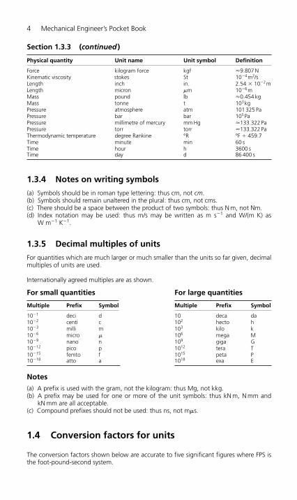
Section 1.3.3 (continued )
Physical quantity Unit name Unit symbol Definition
Force kilogram force kgf �9.807 NKinematic viscosity stokes St 10�4m2/sLength inch in. 2.54 � 10�2mLength micron �m 10�6mMass pound lb �0.454 kgMass tonne t 103kgPressure atmosphere atm 101 325 PaPressure bar bar 105PaPressure millimetre of mercury mm Hg �133.322 PaPressure torr torr �133.322 PaThermodynamic temperature degree Rankine °R °F � 459.7Time minute min 60 sTime hour h 3600 sTime day d 86 400 s
1.3.4 Notes on writing symbols
(a) Symbols should be in roman type lettering: thus cm, not cm.(b) Symbols should remain unaltered in the plural: thus cm, not cms.(c) There should be a space between the product of two symbols: thus N m, not Nm.(d) Index notation may be used: thus m/s may be written as m s�1 and W/(m K) as
W m�1 K�1.
1.3.5 Decimal multiples of units
For quantities which are much larger or much smaller than the units so far given, decimalmultiples of units are used.
Internationally agreed multiples are as shown.
For small quantities For large quantities
Multiple Prefix Symbol Multiple Prefix Symbol
10�1 deci d 10 deca da10�2 centi c 102 hecto h10�3 milli m 103 kilo k10�6 micro � 106 mega M10�9 nano n 109 giga G10�12 pico p 1012 tera T10�15 femto f 1015 peta P10�18 atto a 1018 exa E
Notes(a) A prefix is used with the gram, not the kilogram: thus Mg, not kkg.(b) A prefix may be used for one or more of the unit symbols: thus kN m, N mm and
kN mm are all acceptable.(c) Compound prefixes should not be used: thus ns, not m�s.
1.4 Conversion factors for units
The conversion factors shown below are accurate to five significant figures where FPS isthe foot-pound-second system.
4 Mechanical Engineer’s Pocket Book
H6508-Ch01.qxd 9/12/05 4:39 PM Page 4
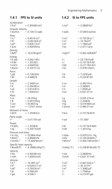
1.4.1 FPS to SI units 1.4.2 SI to FPS units
Acceleration1 ft /s2 0.304 80 m/s2 1 m/s2 3.2808 ft/s2
Angular velocity1 rev/min 0.104 72 rad/s 1 rad/s 9.5493 rev/min
Area1 in.2 6.4516 cm2 1 cm2 0.155 00 in.2
1 ft2 0.092 903 m2 1 m2 10.764 ft2
1 yd2 0.836 13 m2 1 m2 1.1960 yd2
1 acre 0.404 69 ha 1 ha 2.4711 acreDensity1 lb/ft3 16.018 kg/m3 1 kg/m3 0.062 428 lb/ft3
Energy1 ft pdl 0.042 140 J 1 J 23.730 ft pdl1 ft lbf 1.355 82 J 1 J 0.737 56 ft lbf1 k W h 3.6000 MJ 1 MJ 0.277 78 k W h1 therm 0.105 51 GJ 1 GJ 9.4781 thermForce1 pdl 0.138 26 N 1 N 7.2330 pdl1 lbf 4.4482 N 1 N 0.224 81 lbfLength1 in. 2.5400 cm 1 cm 0.393 70 in.1 ft 0.304 80 m 1 m 3.2808 ft1 yd 0.914 40 m 1 m 1.0936 yd1 mi 1.6093 km 1 km 0.621 37 miMass1 oz 28.350 g 1 g 0.035 274 oz1 lb 0.453 59 kg 1 kg 2.2046 lb1 cwt 50.802 kg 1 kg 0.019 684 cwt1 ton 1.0161 tonne 1 tonne 0.984 21 ton
Moment of force1 lbf ft 1.3558 N m 1 N m 0.737 56 lbf ft
Plane angle1° 0.017 45 rad 1 rad 57.296°
Power1 ft lbf/s 1.3558 W 1 W 0.737 56 ft lbf/s1 hp 0.745 70 kW 1 kW 1.3410 hpPressure and stress1 in. Hg 33.864 mbar 1 mbar 0.029 53 in. Hg1 lbf/in.2 6.8948 kPa 1 kPa 0.145 04 lbf/in.2
1 tonf/in.2 15.444 N/mm2 1 N/mm2 0.064 749 tonf/in.2
Specific heat capacity1 Btu/(lb°F) 4.1868 kJ/(kg°C) 1 kJ/(kg °C) 0.238 85 Btu/(lb °F)
Velocity1 ft/s 0.304 80 m/s 1 m/s 3.2808 ft/s1 mi/h 1.6093 km/h 1 km/h 0.621 37 mi/hVolume1 in.3 16.387 cm3 1 cm3 0.061 024 in.3
1 ft3 0.028 317 m3 1 m3 35.315 ft3
1 yd3 0.764 56 m3 1 m3 1.3080 yd3
1 pt 0.568 26 l 1 l 1.7598 pt1 gal 4.5461 l 1 l 0.219 97 gal
Engineering Mathematics 5
H6508-Ch01.qxd 9/12/05 4:39 PM Page 5
1.5 Preferred numbers
When one is buying, say, an electric lamp for use in the home, the normal range of lampsavailable is 15, 25, 40, 60, 100 W and so on. These watt values approximately follow ageometric progression, roughly giving a uniform percentage change in light emissionbetween consecutive sizes. In general, the relationship between the sizes of a commodityis not random but based on a system of preferred numbers.
Preferred numbers are based on R numbers devised by Colonel Charles Renard. The principalseries used are R5, R10, R20, R40 and R80, and subsets of these series. The values within aseries are approximate geometric progressions based on common ratios of 5�–––1–0, 10�–1–0, 20�–1–0,40�–1–0 and 80�–1–0, representing changes between various sizes within a series of 58% for theR5 series, 26% for the R10, 12% for the R20, 6% for the R40 and 3% for the R80 series.
Further details on the values and use of preferred numbers may be found in BS 2045:1965.The rounded values for the R5 series are given as 1.00, 1.60, 2.50, 4.00, 6.30 and 10.00;these values indicate that the electric lamp sizes given above are based on the R5 series.Many of the standards in use are based on series of preferred numbers and these includesuch standards as sheet and wire gauges, nut and bolt sizes, standard currents (A) androtating speeds of machine tool spindles.
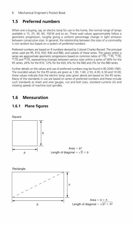
1.6 Mensuration
1.6.1 Plane figures
6 Mechanical Engineer’s Pocket Book
Area b2
Length of diagonal √2 � bb
b
Square
Area b � hLength of diagonal √b2 � h2
Rectangle
b
h
H6508-Ch01.qxd 9/12/05 4:39 PM Page 6

Engineering Mathematics 7
Area b � h
h
Parallelogram
b
Trapeziuma
b
hArea � (a � b) � h1
2
b
h
Triangle
Area � b � h12
Circle
r
Area p � r 2
Perimeter 2 � p � r
H6508-Ch01.qxd 9/12/05 4:39 PM Page 7

8 Mechanical Engineer’s Pocket Book
Sector of circle
s
r
u
aArea p � a � b
Perimeter p � (a � b)
Ellipse
Irregular plane
Datum
r
t
uv
wp
u
d
s
r
x2x1
q
b
Arc length s r � u
(u is in radians)
Area � r 2 � u12
H6508-Ch01.qxd 9/12/05 4:39 PM Page 8

Several methods are used to find the shaded area, such as the mid-ordinate rule, the trapez-oidal rule and Simpson’s rule. As an example of these, Simpson’s rule is as shown. Dividex1x2 into an even number of equal parts of width d. Let p, q, r, … be the lengths of verti-cal lines measured from some datum, and let A be the approximate area of the irregularplane, shown shaded. Then:
In general, the statement of Simpson’s rule is:
where first, last, evens, odds refer to ordinate lengths and d is the width of the equal partsof the datum line.
1.6.2 Solid objects
Approximate area (d/3) [(first last) 4(sum � � � oof evens) 2(sum of odds)]�
Ad
p t q s rd
p t u w v � � � � � � � � �3
[( ) 4( ) 2 ]3
[( ) 4( ) 2
b
lh
Rectangular prism
Total surface area 2(bh � hl � lb)
Volume bhl
Cylinder
Volume pr 2hTotal surface area 2pr (r �h)r
h
Engineering Mathematics 9
H6508-Ch01.qxd 9/12/05 4:39 PM Page 9

10 Mechanical Engineer’s Pocket Book
Cone
Volume (1/3)pr 2hTotal surface area pr (l � r)
hl
r
Sphere
rVolume (4/3) pr 3
Total surface area 4pr 2
Frustrum of cone
Volume (1/3)ph(R 2 � Rr � r 2)Total surface area pl (R � r )�p(R 2 � r 2)
r
hl
R
H6508-Ch01.qxd 9/12/05 4:39 PM Page 10
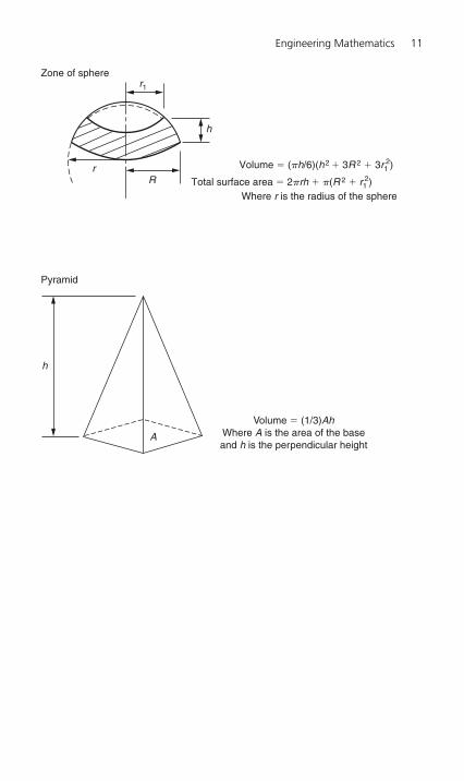
Engineering Mathematics 11
Pyramid
h
A
Volume (1/3)AhWhere A is the area of the baseand h is the perpendicular height
Rr
h
Zone of spherer1
Volume (ph/6)(h2 � 3R 2 � 3r12)
Total surface area 2prh � p(R 2 � r12)
Where r is the radius of the sphere
H6508-Ch01.qxd 9/12/05 4:39 PM Page 11
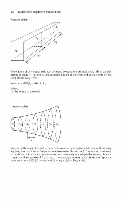
12 Mechanical Engineer’s Pocket Book
Irregular solids
d
A1 A2 A3 A4 A5 A6 A7
Various methods can be used to determine volumes of irregular solids; one of these is byapplying the principles of Simpson’s rule (see earlier this section). The solid is consideredto be divided into an even number of sections by equally spaced, parallel planes, distanced apart and having areas of A1, A2, A3, …. Assuming, say, seven such planes, then approxi-mate volume (d/3) [(A1 � A7) � 4(A2 � A4 � A6) � 2(A3 � A5)].
The volume of any regular solid can be found by using the prismoidal rule. Three parallelplanes of areas A1, A3 and A2 are considered to be at the ends and at the centre of thesolid, respectively. Then:
Where:l is the length of the solid.
Volume ( ( 4 )1 2 3 � �l A A A/ )6
Regular solids
A1
A2
l /2
l /2
A3
H6508-Ch01.qxd 9/12/05 4:39 PM Page 12
Engineering Mathem
atics13
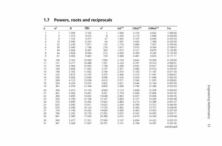
1.7 Powers, roots and reciprocals
n n2 �n–– �10n—–– n3 (n)1/3 (10n)1/3 (100n)1/3 1/n
1 1 1.000 3.162 1 1.000 2.154 4.642 1.000 002 4 1.414 4.472 8 1.260 2.714 5.848 0.500 003 9 1.732 5.477 27 1.442 3.107 6.694 0.333 334 16 2.000 6.325 64 1.587 3.420 7.368 0.250 005 25 2.236 7.071 125 1.710 3.684 7.937 0.200 006 36 2.449 7.746 216 1.817 3.915 8.434 0.166 677 49 2.646 8.367 343 1.913 4.121 8.879 0.142 868 64 2.828 8.944 512 2.000 4.309 9.283 0.125 009 81 3.000 9.487 729 2.080 4.481 9.655 0.111 11
10 100 3.162 10.000 1 000 2.154 4.642 10.000 0.100 0011 121 3.317 10.488 1 331 2.224 4.791 10.323 0.090 9112 144 3.464 10.954 1 738 2.289 4.932 10.627 0.083 3313 169 3.606 11.402 2 197 2.351 5.066 10.914 0.076 9214 196 3.742 11.832 2 744 2.410 5.192 11.187 0.071 4315 225 3.873 12.247 3 375 2.466 5.313 11.447 0.066 6716 256 4.000 12.649 4 096 2.520 5.429 11.696 0.062 5017 289 4.123 13.038 4 913 2.571 5.540 11.935 0.058 8218 324 4.243 13.416 5 832 2.621 5.646 12.164 0.055 5619 361 4.359 13.784 6 859 2.668 5.749 12.386 0.052 63
20 400 4.472 14.142 8 000 2.714 5.848 12.599 0.050 0021 441 4.583 14.491 9 261 2.759 5.944 12.806 0.047 6222 484 4.690 14.832 10 648 2.802 6.037 13.006 0.045 4523 529 4.796 15.166 12 167 2.844 6.127 13.200 0.043 4824 576 4.899 15.492 13 824 2.884 6.214 13.389 0.041 6725 625 5.000 15.811 15 625 2.924 6.300 13.572 0.040 0026 676 5.099 16.125 17 576 2.962 6.383 13.751 0.038 4627 729 5.196 16.432 19 683 3.000 6.463 13.925 0.037 0428 784 5.292 16.733 21 952 3.037 6.542 14.095 0.035 7129 841 5.385 17.029 24 389 3.072 6.619 14.260 0.034 48
30 900 5.477 17.321 27 000 3.107 6.694 14.422 0.033 3331 961 5.568 17.607 29 791 3.141 6.768 14.581 0.032 26
continued
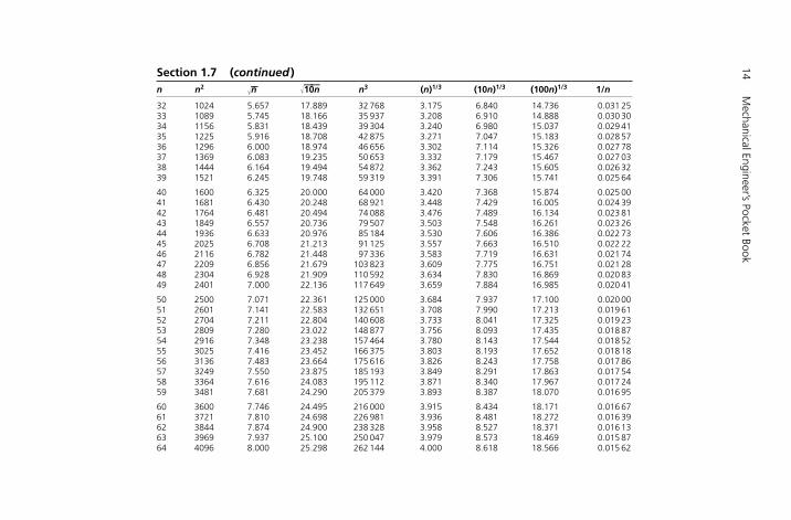
14M
echanical Engineer’s Pocket Book
Section 1.7 (continued )n n2 �n–– �10n—–– n3 (n)1/3 (10n)1/3 (100n)1/3 1/n
32 1024 5.657 17.889 32 768 3.175 6.840 14.736 0.031 2533 1089 5.745 18.166 35 937 3.208 6.910 14.888 0.030 3034 1156 5.831 18.439 39 304 3.240 6.980 15.037 0.029 4135 1225 5.916 18.708 42 875 3.271 7.047 15.183 0.028 5736 1296 6.000 18.974 46 656 3.302 7.114 15.326 0.027 7837 1369 6.083 19.235 50 653 3.332 7.179 15.467 0.027 0338 1444 6.164 19.494 54 872 3.362 7.243 15.605 0.026 3239 1521 6.245 19.748 59 319 3.391 7.306 15.741 0.025 64
40 1600 6.325 20.000 64 000 3.420 7.368 15.874 0.025 0041 1681 6.430 20.248 68 921 3.448 7.429 16.005 0.024 3942 1764 6.481 20.494 74 088 3.476 7.489 16.134 0.023 8143 1849 6.557 20.736 79 507 3.503 7.548 16.261 0.023 2644 1936 6.633 20.976 85 184 3.530 7.606 16.386 0.022 7345 2025 6.708 21.213 91 125 3.557 7.663 16.510 0.022 2246 2116 6.782 21.448 97 336 3.583 7.719 16.631 0.021 7447 2209 6.856 21.679 103 823 3.609 7.775 16.751 0.021 2848 2304 6.928 21.909 110 592 3.634 7.830 16.869 0.020 8349 2401 7.000 22.136 117 649 3.659 7.884 16.985 0.020 41
50 2500 7.071 22.361 125 000 3.684 7.937 17.100 0.020 0051 2601 7.141 22.583 132 651 3.708 7.990 17.213 0.019 6152 2704 7.211 22.804 140 608 3.733 8.041 17.325 0.019 2353 2809 7.280 23.022 148 877 3.756 8.093 17.435 0.018 8754 2916 7.348 23.238 157 464 3.780 8.143 17.544 0.018 5255 3025 7.416 23.452 166 375 3.803 8.193 17.652 0.018 1856 3136 7.483 23.664 175 616 3.826 8.243 17.758 0.017 8657 3249 7.550 23.875 185 193 3.849 8.291 17.863 0.017 5458 3364 7.616 24.083 195 112 3.871 8.340 17.967 0.017 2459 3481 7.681 24.290 205 379 3.893 8.387 18.070 0.016 95
60 3600 7.746 24.495 216 000 3.915 8.434 18.171 0.016 6761 3721 7.810 24.698 226 981 3.936 8.481 18.272 0.016 3962 3844 7.874 24.900 238 328 3.958 8.527 18.371 0.016 1363 3969 7.937 25.100 250 047 3.979 8.573 18.469 0.015 8764 4096 8.000 25.298 262 144 4.000 8.618 18.566 0.015 62
Engineering Mathem
atics15
65 4225 8.062 25.495 274 625 4.021 8.662 18.663 0.015 3866 4356 8.124 25.690 287 496 4.041 8.707 18.758 0.015 1567 4489 8.185 25.884 300 763 4.062 8.750 18.852 0.014 9368 4624 8.246 26.077 314 432 4.082 8.794 18.945 0.014 7169 4761 8.307 26.268 328 509 4.102 8.837 19.038 0.014 49
70 4900 8.367 26.458 343 000 4.121 8.879 19.129 0.014 2971 5041 8.426 26.646 357 911 4.141 8.921 19.220 0.014 0872 5184 8.485 26.833 373 248 4.160 8.963 19.310 0.013 8973 5329 8.544 27.019 389 017 4.179 9.004 19.399 0.013 7074 5476 8.602 27.203 405 224 4.198 9.045 19.487 0.013 5175 5625 8.660 27.386 421 875 4.217 9.086 19.574 0.013 3376 5776 8.718 27.568 438 976 4.236 9.126 19.661 0.013 1677 5929 8.775 27.749 456 533 4.254 9.166 19.747 0.012 9978 6084 8.832 27.928 474 552 4.273 9.205 19.832 0.012 8279 6241 8.888 28.107 493 039 4.291 9.244 19.916 0.012 66
80 6400 8.944 28.284 512 000 4.309 9.283 20.000 0.012 5081 6561 9.000 28.460 531 441 4.327 9.322 20.083 0.012 3582 6724 9.055 28.636 551 368 4.344 9.360 20.165 0.012 2083 6889 9.110 28.810 571 787 4.362 9.398 20.247 0.012 0584 7056 9.165 28.983 592 704 4.380 9.435 20.328 0.011 9085 7225 9.220 29.155 614 125 4.397 9.473 20.408 0.011 7686 7396 9.274 29.326 636 056 4.414 9.510 20.488 0.011 6387 7569 9.327 29.496 658 503 4.431 9.546 20.567 0.011 4988 7744 9.381 29.665 681 472 4.448 9.583 20.646 0.011 3689 7921 9.434 29.833 704 969 4.465 9.619 20.724 0.011 24
90 8100 9.487 30.000 729 000 4.481 9.655 20.801 0.011 1191 8281 9.539 30.166 753 571 4.498 9.691 20.878 0.010 9992 8464 9.592 30.332 778 688 4.514 9.726 20.954 0.010 8793 8649 9.644 30.496 804 357 4.531 9.761 21.029 0.010 7594 8836 9.695 30.659 830 584 4.547 9.796 21.105 0.010 6495 9025 9.747 30.822 857 375 4.563 9.830 21.179 0.010 5396 9216 9.798 30.984 884 736 4.579 9.865 21.253 0.010 4297 9409 9.849 31.145 912 673 4.595 9.899 21.327 0.010 3198 9604 9.899 31.305 941 192 4.610 9.933 21.400 0.010 2099 9801 9.950 31.464 970 299 4.626 9.967 21.472 0.010 10

16 Mechanical Engineer’s Pocket Book
1.8 Progressions
A set of numbers in which one number is connected to the next number by some law iscalled a series or a progression.
1.8.1 Arithmetic progressions
The relationship between consecutive numbers in an arithmetic progression is that they areconnected by a common difference. For the set of numbers 3, 6, 9, 12, 15, …, the series isobtained by adding 3 to the preceding number; that is, the common difference is 3. In gen-eral, when a is the first term and d is the common difference, the arithmetic progression isof the form:
Term 1st 2nd 3rd 4th lastValue a a � d a � 2d a � 3d, … a � (n � 1)d
where: n is the number of terms in the progression.
The sum Sn of all the terms is given by the average value of the terms times the numberof terms; that is:
Sn [(first � last)/2] � (number of terms)
[(a � a � (n � 1)d)/2] � n
(n/2)[2a � (n � 1)d]
1.8.2 Geometric progressions
The relationship between consecutive numbers in a geometric progression is that they areconnected by a common ratio. For the set of numbers 3, 6, 12, 24, 48, …, the series isobtained by multiplying the preceding number by 2. In general, when a is the first termand r is the common ratio, the geometric progression is of the form:
Term 1st 2nd 3rd 4th lastValue a ar ar2 ar3, … arn�1
where:n is the number of terms in the progression.
The sum Sn of all the terms may be found as follows:
Sn a � ar � ar2 � ar3 � … � arn�1 (1)
Multiplying each term of equation (1) by r gives
rSn ar � ar2 � ar3 � … � arn�1 � arn (2)
Subtracting equations (2) from (1) gives:
Sn(1 � r) a � arn (3)Sn [a(1 � rn)]/(1 � r)
H6508-Ch01.qxd 9/12/05 4:39 PM Page 16

Engineering Mathematics 17
Alternatively, multiplying both numerator and denominator by �1 gives:
Sn [a(rn � 1)]/(r � 1) (4)
It is usual to use equation (3) when r 1 and (4) when r � 1.
When �1 � r � 1, each term of a geometric progression is smaller than the precedingterm and the terms are said to converge. It is possible to find the sum of all the terms ofa converging series. In this case, such a sum is called the sum to infinity. The term[a(1 � r n)]/(1 � r) can be rewritten as [a/(1 � r)] � [arn/(1 � r)]. Since r is less than 1, r n
becomes smaller and smaller as n grows larger and larger. When n is very large, rn effect-ively becomes zero, and thus [arn/(1 � r)] becomes zero. It follows that the sum to infin-ity of a geometric progression is a/(1 � r), which is valid when �1 � r � 1.
1.8.3 Harmonic progressions
The relationship between numbers in a harmonic progression is that the reciprocals ofconsecutive terms form an arithmetic progression. Thus for the arithmetic progression 1, 2, 3, 4, 5, …, the corresponding harmonic progression is 1, 1/2, 1/3, 1/4, 1/5, ….
1.9 Trigonometric formulae
1.9.1 Basic definitions
In the right-angled triangle shown below, a is the side opposite to angle A, b is thehypotenuse of the triangle and c is the side adjacent to angle A. By definition:
sin A opp/hyp a/b
cos A adj/hyp c/b
tan A opp/adj a/c
cosec A hyp/opp b/a 1/sin A
sec A hyp/adj b/c 1/cos A
cot A adj/opp c/a 1/tan A
B A
C
aopp
cadj
bhyp
H6508-Ch01.qxd 9/12/05 4:39 PM Page 17
18 Mechanical Engineer’s Pocket Book
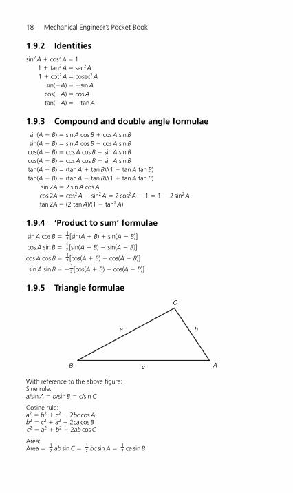
1.9.2 Identities
sin2A � cos2A 11 � tan2A sec2A1 � cot2A cosec2A
sin(�A) �sin Acos(�A) cos Atan(�A) �tan A
1.9.3 Compound and double angle formulae
sin(A � B) sin A cos B � cos A sin Bsin(A � B) sin A cos B � cos A sin Bcos(A � B) cos A cos B � sin A sin Bcos(A � B) cos A cos B � sin A sin Btan(A � B) (tan A � tan B)/(1 � tan A tan B)tan(A � B) (tan A � tan B)/(1 � tan A tan B)
sin 2A 2 sin A cos Acos 2A cos2A � sin2A 2 cos2A � 1 1 � 2 sin2Atan 2A (2 tan A)/(1 � tan2A)
1.9.4 ‘Product to sum’ formulae
sin A cos B [sin(A � B) � sin(A � B)]
cos A sin B [sin(A � B) � sin(A � B)]
cos A cos B [cos(A � B) � cos(A � B)]
sin A sin B � [cos(A � B) � cos(A � B)]
1.9.5 Triangle formulae
12
12
12
12
C
AB c
a b
With reference to the above figure:Sine rule:a/sin A b/sin B c/sin C
Cosine rule:a2 b2 � c2 � 2bc cos Ab2 c2 � a2 � 2ca cos Bc2 a2 � b2 � 2ab cos C
Area:Area ab sin C bc sin A ca sin B
12
12
12
H6508-Ch01.qxd 9/12/05 4:39 PM Page 18

Engineering Mathematics 19
Also:
where:s is the semi-perimeter, that is, (a � b � c)/2.
1.10 Circles: some definitions and properties
For a circle of diameter d and radius r:
The circumference is �d or 2�r.
The area is �d2/4 or �r2.
An arc of a circle is part of the circumference.
A tangent to a circle is a straight line which meets the circle at one point only. A radiusdrawn from the point where a tangent meets a circle is at right angles to the tangent.
A sector of a circle is the area between an arc of the circle and two radii. The area of asector is r2�, where � is the angle in radians between the radii.
A chord is a straight line joining two points on the circumference of a circle. When twochords intersect, the product of the parts of one chord is equal to the products of theparts of the other chord. In the following figure, AE � BE CE � ED.
12
Area ( )( )( ) � � �s s a s a s c
E
B
D
C
A
A
B
A segment of a circle is the area bounded by a chord and an arc. Angles in the same segment of a circle are equal: in the following figure, angle A angle B.
H6508-Ch01.qxd 9/12/05 4:39 PM Page 19
20M
echanical Engineer’s Pocket Book
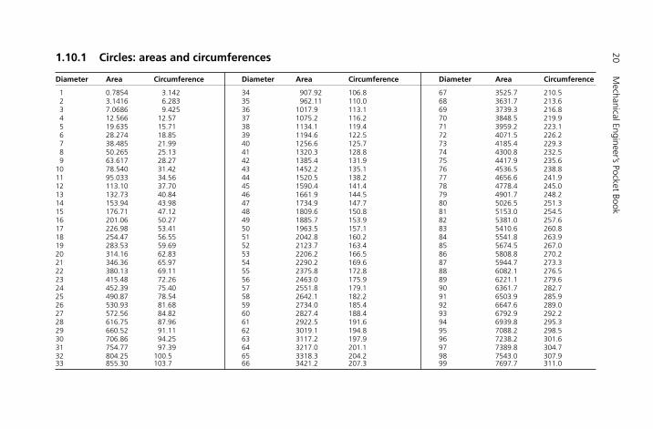
1.10.1 Circles: areas and circumferences
Diameter Area Circumference Diameter Area Circumference Diameter Area Circumference
1 0.7854 3.142 34 907.92 106.8 67 3525.7 210.52 3.1416 6.283 35 962.11 110.0 68 3631.7 213.63 7.0686 9.425 36 1017.9 113.1 69 3739.3 216.84 12.566 12.57 37 1075.2 116.2 70 3848.5 219.95 19.635 15.71 38 1134.1 119.4 71 3959.2 223.16 28.274 18.85 39 1194.6 122.5 72 4071.5 226.27 38.485 21.99 40 1256.6 125.7 73 4185.4 229.38 50.265 25.13 41 1320.3 128.8 74 4300.8 232.59 63.617 28.27 42 1385.4 131.9 75 4417.9 235.6
10 78.540 31.42 43 1452.2 135.1 76 4536.5 238.811 95.033 34.56 44 1520.5 138.2 77 4656.6 241.912 113.10 37.70 45 1590.4 141.4 78 4778.4 245.013 132.73 40.84 46 1661.9 144.5 79 4901.7 248.214 153.94 43.98 47 1734.9 147.7 80 5026.5 251.315 176.71 47.12 48 1809.6 150.8 81 5153.0 254.516 201.06 50.27 49 1885.7 153.9 82 5381.0 257.617 226.98 53.41 50 1963.5 157.1 83 5410.6 260.818 254.47 56.55 51 2042.8 160.2 84 5541.8 263.919 283.53 59.69 52 2123.7 163.4 85 5674.5 267.020 314.16 62.83 53 2206.2 166.5 86 5808.8 270.221 346.36 65.97 54 2290.2 169.6 87 5944.7 273.322 380.13 69.11 55 2375.8 172.8 88 6082.1 276.523 415.48 72.26 56 2463.0 175.9 89 6221.1 279.624 452.39 75.40 57 2551.8 179.1 90 6361.7 282.725 490.87 78.54 58 2642.1 182.2 91 6503.9 285.926 530.93 81.68 59 2734.0 185.4 92 6647.6 289.027 572.56 84.82 60 2827.4 188.4 93 6792.9 292.228 616.75 87.96 61 2922.5 191.6 94 6939.8 295.329 660.52 91.11 62 3019.1 194.8 95 7088.2 298.530 706.86 94.25 63 3117.2 197.9 96 7238.2 301.631 754.77 97.39 64 3217.0 201.1 97 7389.8 304.732 804.25 100.5 65 3318.3 204.2 98 7543.0 307.933 855.30 103.7 66 3421.2 207.3 99 7697.7 311.0

1.11 Quadratic equations
The solutions (roots) of a quadratic equation:
ax2 � bx � c 0
are:
x
1.12 Natural logarithms
The natural logarithm of a positive real number x is denoted by ln x. It is defined to be anumber such that:
eln x x
where:e 2.1782 which is the base of natural logarithms.
Natural logarithms have the following properties:
ln(xy) ln x � ln y
ln(x/y) ln x � ln y
ln yx x ln y
1.13 Statistics: an introduction
1.13.1 Basic concepts
To understand the fairly advanced statistics underlying quality control, a certain basic levelof statistics is assumed by most texts dealing with this subject. The brief introduction givenbelow should help to lead readers into the various texts dealing with quality control.
The arithmetic mean, or mean, is the average value of a set of data. Its value can be foundby adding together the values of the members of the set and then dividing by the num-ber of members in the set. Mathematically:
X (X1 � X2 � … � XN)/N
Thus the mean of the set of numbers 4, 6, 9, 3 and 8 is (4 � 6 � 9 � 3 � 8)/5 6.
The median is either the middle value or the mean of the two middle values of a set ofnumbers arranged in order of magnitude. Thus the numbers 3, 4, 5, 6, 8, 9, 13 and 15have a median value of (6 � 8)/2 7, and the numbers 4, 5, 7, 9, 10, 11, 15, 17 and 19have a median value of 10.
The mode is the value in a set of numbers which occurs most frequently. Thus the set 2,3, 3, 4, 5, 6, 6, 6, 7, 8, 9 and 9 has a modal value of 6.
� � �b b aca
2 42
Engineering Mathematics 21
H6508-Ch01.qxd 9/12/05 4:39 PM Page 21
22 Mechanical Engineer’s Pocket Book
The range of a set of numbers is the difference between the largest value and the smallestvalue. Thus the range of the set of numbers 3, 2, 9, 7, 4, 1, 12, 3, 17 and 4 is 17 � 1 16.
The standard deviation, sometimes called the root mean square deviation, is defined by:
Thus for the numbers 2, 5 and 11, the mean in (2 � 5 � 11)/3, that is 6. The standarddeviation is:
Usually s is used to denote the standard deviation of a population (the whole set of val-ues) and � is used to denote the standard deviation of a sample.
1.13.2 Probability
When an event can happen x ways out of a total of n possible and equally likely ways, theprobability of the occurrence of the event is given by p x/n. The probability of an eventoccurring is therefore a number between 0 and 1. If q is the probability of an event notoccurring it also follows that p � q 1. Thus when a fair six-sided dice is thrown, theprobability of getting a particular number, say a three, is 1/6, since there are six sides andthe number three only appears on one of the six sides.
1.13.3 Binomial distribution
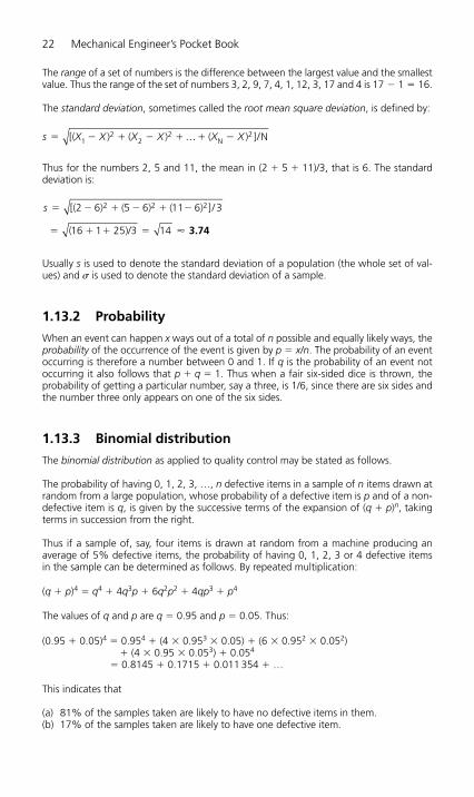
The binomial distribution as applied to quality control may be stated as follows.
The probability of having 0, 1, 2, 3, …, n defective items in a sample of n items drawn atrandom from a large population, whose probability of a defective item is p and of a non-defective item is q, is given by the successive terms of the expansion of (q � p)n, takingterms in succession from the right.
Thus if a sample of, say, four items is drawn at random from a machine producing anaverage of 5% defective items, the probability of having 0, 1, 2, 3 or 4 defective items in the sample can be determined as follows. By repeated multiplication:
(q � p)4 q4 � 4q3p � 6q2p2 � 4qp3 � p4
The values of q and p are q 0.95 and p 0.05. Thus:
(0.95 � 0.05)4 0.954 � (4 � 0.953 � 0.05) � (6 � 0.952 � 0.052)� (4 � 0.95 � 0.053) � 0.054
0.8145 � 0.1715 � 0.011 354 � …
This indicates that
(a) 81% of the samples taken are likely to have no defective items in them.(b) 17% of the samples taken are likely to have one defective item.
� � (16 1 25)/3 14 � 3.74
s � � � � �[( ( (2 5 116) 6) 6) ]/ 32 2 2
s X X X X X X � � � � � �[( ) ( ) ( ) N12
22
N2… ] /
H6508-Ch01.qxd 9/12/05 4:39 PM Page 22

Engineering Mathematics 23
(c) 1% of the samples taken are likely to have two defective items.(d) There will hardly ever be three or four defective items in a sample.
As far as quality control is concerned, if by repeated sampling these percentages areroughly maintained, the inspector is satisfied that the machine is continuing to produceabout 5% defective items. However, if the percentages alter then it is likely that thedefect rate has also altered. Similarly, a customer receiving a large batch of items can, byrandom sampling, find the number of defective items in the samples and by using the binomial distribution can predict the probable number of defective items in the whole batch.
1.13.4 Poisson distribution
The calculations involved in a binomial distribution can be very long when the samplenumber n is larger than about six or seven, and an approximation to them can beobtained by using a Poisson distribution. A statement for this is:
When the chance of an event occurring at any instant is constant and the expectation npof the event occurring is �, then the probabilities of the event occurring 0, 1, 2, 3, 4, …times are given by:
e��, �e��, �2e��/2!, �3e��/3!, �4e��/4!, …
where:e is the constant 2.718 28 … and 2! 2 � 1, 3! 3 � 2 � 1, 4! 4 � 3 � 2 � 1, andso on (where 4! is read ‘four factorial’).
Applying the Poisson distribution statement to the machine producing 5% defectiveitems, used above to illustrate a use of the binomial distribution, gives:
expectation np 4 � 0.05 0.2probability of no defective items is e�� e�0.2 0.8187probability of one defective item is �e�� 0.2e�0.2 0.1637probability of two defective items is �2e��/2! 0.22e�0.2/2 0.0164
It can be seen that these probabilities of approximately 82%, 16% and 2% comparequite well with the results obtained previously.
1.13.5 Normal distribution
Data associated with measured quantities such as mass, length, time and temperature iscalled continuous, that is, the data can have any values between certain limits. Supposethat the lengths of items produced by a certain machine tool were plotted as a graph, asshown in the figure; then it is likely that the resulting shape would be mathematicallydefinable. The shape is given by y (1/�)ez, where z �x2/2�2, � is the standard deviationof the data, and x is the frequency with which the data occurs. Such a curve is called anormal probability or a normal distribution curve.
Important properties of this curve to quality control are:
(a) The area enclosed by the curve and vertical lines at �1 standard deviation from themean value is approximately 67% of the total area.
H6508-Ch01.qxd 9/12/05 4:39 PM Page 23
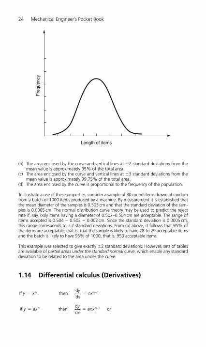
24 Mechanical Engineer’s Pocket Book
(b) The area enclosed by the curve and vertical lines at �2 standard deviations from themean value is approximately 95% of the total area.
(c) The area enclosed by the curve and vertical lines at �3 standard deviations from themean value is approximately 99.75% of the total area.
(d) The area enclosed by the curve is proportional to the frequency of the population.
To illustrate a use of these properties, consider a sample of 30 round items drawn at randomfrom a batch of 1000 items produced by a machine. By measurement it is established thatthe mean diameter of the samples is 0.503 cm and that the standard deviation of the sam-ples is 0.0005 cm. The normal distribution curve theory may be used to predict the rejectrate if, say, only items having a diameter of 0.502–0.504 cm are acceptable. The range ofitems accepted is 0.504 � 0.502 0.002 cm. Since the standard deviation is 0.0005 cm,this range corresponds to �2 standard deviations. From (b) above, it follows that 95% ofthe items are acceptable, that is, that the sample is likely to have 28 to 29 acceptable itemsand the batch is likely to have 95% of 1000, that is, 950 acceptable items.
This example was selected to give exactly �2 standard deviations. However, sets of tablesare available of partial areas under the standard normal curve, which enable any standarddeviation to be related to the area under the curve.
1.14 Differential calculus (Derivatives)
If thendd
or1y axyx
anxn n �
If thendd
1y xyx
nxn n �
Length of items
Fre
quen
cy
H6508-Ch01.qxd 9/12/05 4:39 PM Page 24

Engineering Mathematics 25
If ln thendd
1y x
yx x
If thendd
lny ayx
a ax x
If e thendd
eyyx
aax ax
If e thendd
eyyx
x x
If cosec thendd
1
2 2y
xa
yx
a
x x a �
�
�
If sec thendd
1
2 2y
xa
yx
a
x x a
�
�
If cot thendd
12 2
yxa
yx
a
a x �
��
If tan thendd
12 2
yxa
yx
a
a x
��
If cos thendd
11
2 2y
xa
yx a x
��
�
If sin thendd
11
2 2y
xa
yx a x
�
�
If cosec thendd
cot coseccos
sin2y
y � �u
uu u
u
u
If sec thendd
tan secsin
cos2y
y u
uu u
u
u
If cot thendd
cosec2yy
uu
u
If tan thendd
sec2yy
uu
u
If cos thendd
sinyy
�uu
u
If sin thendd
cosyy
uu
u
If ( ) then ( )f x ax f x anxn n � �1
H6508-Ch01.qxd 9/12/05 4:39 PM Page 25

Product rule
Quotient rule
Function of a function
Successive differentiation
If y f(x) then its first derivative is written or f�(x).
If this expression is differentiated a second time then the second derivative is obtained
and is written or f�(x).
1.15 Integral calculus (Standard forms)
(n � �1)
Where:c the constant of integration.
(n � �1)
cot cosec d cosecu u u u∫ � � c
tan sec d secu u u u∫ � c
cosec d cot2u u u∫ � � c
sec d tan2u u u∫ � c
sin d cosu u u∫ � � c
cos d sinu u u∫ � c
ax xaxn
cnn
∫ d1
1
��
�
x xxn
cnn
∫ d1
1
��
�
d
d
2
2
y
x
ddyx
If is a function of thendd
dd
dd
y xyx
yu
ux
�
If where and are both functions ofyuv
u v , thendd
dd
dd
2x
yx
vux
uvx
v
�
If where and are both functions ofy uv u v , thendd
dd
dd
xyx
uvx
vux
�
26 Mechanical Engineer’s Pocket Book
H6508-Ch01.qxd 9/12/05 4:39 PM Page 26

Engineering Mathematics 27
d 1or
12
ln( )( )2 2
x
a x axa
ca
a xa x
c�
��
��∫ tanh
dcosh or ln
2 2
12 2x
x a
xa
cx x a
ac
� �
���∫
⎡
⎣
⎢⎢⎢
⎤
⎦
⎥⎥⎥
dsinh or ln
2 2
12 2x
a x
xa
cx x a
ac
� �
� ���∫
⎡
⎣
⎢⎢⎢
⎤
⎦
⎥⎥⎥
sech d tanh2∫ x x x c �
cosh d sinh∫ x x x c �
sinh d cosh∫ x x x c �
dln
xx
x c∫ �
a xax
acx∫ d
ln �
eeax
ax
ac∫ �
e d ex xx c∫ �
�
� ��a x
x x a
xa
cd
cosec 1
2 2∫
a x
x x a
xa
cd
sec2
1
� ��
2∫
�
� ��a x
a x
xa
cd
cot 12 2∫
a x
a x
xa
cd
tan 12 2�
��∫
�
� ��d
cos 1x
a x
xa
c2 2∫
dsin 1x
a x
xa
c2 2�
��∫
H6508-Ch01.qxd 9/12/05 4:39 PM Page 27

1.15.1 Integration by parts
1.15.2 Definite integrals
The foregoing integrals contain an arbitrary constant ‘c’ and are called indefinite integrals.
Definite integrals are those to which limits are applied thus: [x]ab (b) � (a), therefore:
Note how the constant of integration (c) is eliminated in a definite integral.
1.16 Binomial theorem
where 3! is factorial 3 and equals 1 � 2 � 3.
1.17 Maclaurin’s theorem
1.18 Taylor’s theorem
For further information on Engineering Mathematics the reader is referred to the followingPocket Book: Newnes Engineering Mathematics Pocket Book, Third Edition, John Bird,0750649925
f x h f x hf xh
f x( ) ( ) ( )2!
( )2
� � � � �� � ……
f x f xfx
f( ) (0) (0)2!
(0)2
� � � �� � ……
( )( 1)
2!( 1)( 2
1 2 2a x a na xn n
a x
n n n
n n n n� � ��
�� �
� �
))3!
3 3a x xn n� � �…
y x xx
c c � �2
1
3 3
1
33
d3
33∫
⎡
⎣
⎢⎢⎢
⎤
⎦
⎥⎥⎥
⎡
⎣
⎢⎢⎢
⎤
⎦
⎥⎥⎥�� �
� � �
13
(9 )13
3c
c c
⎡
⎣
⎢⎢⎢
⎤
⎦
⎥⎥⎥
⎛
⎝⎜⎜⎜⎜
⎞
⎠⎟⎟⎟⎟⎟
8223
u v uv v u cd d � �∫∫
28 Mechanical Engineer’s Pocket Book
H6508-Ch01.qxd 9/12/05 4:39 PM Page 28
2Engineering Statics
2.1 Engineering statics
Engineering mechanics can be divided into statics and dynamics. Basically, statics is thestudy of forces and their effects in equilibrium, whereas dynamics is the study of objectsin motion.
2.2 Mass, force and weight
2.2.1 Mass● Mass is the quantity of matter in a body. It is the sum total of the masses of all the sub-
atomic particles in that body.● Matter occupies space and can be solid, liquid or gaseous.● Unless matter is added to or removed from a body, the mass of that body never varies.
It is constant under all conditions. There are as many atoms in a kilogram of, say, metalon the moon as there are in the same kilogram of metal on planet Earth. However, thatkilogram of metal will weigh less on the moon than on planet Earth (see Section 2.2.4).
● The basic unit of mass is the kilogram (kg). The most commonly used multiple of thisbasic unit is the tonne (1000 kg) and the most commonly used sub-multiple is the gram(0.001 kg).
2.2.2 Force
To understand how mass and weight are related it is necessary to consider the concept offorce. A force or a system of forces cannot be seen; only the effect of a force or a systemof forces can be seen. That is:
● A force can change or try to change the shape of an object.● A force can move or try to move a body that is at rest. If the magnitude of the force is
sufficiently great it will cause the body to move in the direction of the application ofthe force. If the force is of insufficient magnitude to overcome the resistance to move-ment it will still try to move the body, albeit unsuccessfully.
● A force can change or try to change the motion of a body that is already moving. Forexample:1. The force of a headwind can decrease the speed of an aircraft over the ground,
whereas the force of a tailwind can increase the speed of an aircraft over the ground.2. The force of a crosswind can cause a car to swerve off course.
H6508-Ch02.qxd 9/12/05 4:39 PM Page 29
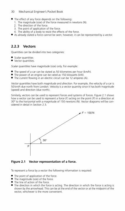
● The effect of any force depends on the following:1. The magnitude (size) of the force measured in newtons (N).2. The direction of the force.3. The point of application of the force.4. The ability of a body to resist the effects of the force.
● As already stated a force cannot be seen; however, it can be represented by a vector.
2.2.3 Vectors
Quantities can be divided into two categories:
● Scalar quantities● Vector quantities.
Scalar quantities have magnitude (size) only. For example:
● The speed of a car can be stated as 50 kilometres per hour (km/h).● The power of an engine can be rated as 150 kilowatts (kW).● The current flowing in an electric circuit can be 12 amperes (A).
Vector quantities have both magnitude and direction. For example, the velocity of a car is50 km/h due north from London. Velocity is a vector quantity since it has both magnitude(speed) and direction (due north).
Similarly, vectors can be used to represent forces and systems of forces. Figure 2.1 showshow a vector can be used to represent a force (F ) acting on the point (P) in a direction at30° to the horizontal with a magnitude of 150 newtons (N). Vector diagrams will be con-sidered in detail in Section 2.3.
30 Mechanical Engineer’s Pocket Book
30°
F � 150 N
P
Figure 2.1 Vector representation of a force.
To represent a force by a vector the following information is required:
● The point of application of the force.● The magnitude (size) of the force.● The line of action of the force.● The direction in which the force is acting. The direction in which the force is acting is
shown by the arrowhead. This can be at the end of the vector or at the midpoint of thevector, whichever is the more convenient.
H6508-Ch02.qxd 9/12/05 4:39 PM Page 30
2.2.4 Weight
A solid, liquid or gas of mass 1 kg will weigh 9.81 N due to the gravitational attraction ofplanet Earth. Since planet Earth is not a perfect sphere a mass of 1 kg will weigh slightlymore at the poles and slightly less at the equator. However, for all practical purposes, theaverage weight of a mass of 1 kg is taken to be 9.81 N on planet Earth:
● The force of gravity attracts the mass of any body (solid, liquid or gas) towards thecentre of planet Earth.
● The weight of a body is the force of gravity acting on that body.● Therefore weight is a force measured in newtons.● The factor 9.81 is the free-fall acceleration of a body due to the force gravity, it is 9.81
metres per second squared (m/s2). Acceleration due to gravity is discussed further inSection 3.6.7.
● Since the weight of a body of mass 1 kg is approximately 9.81 N (average value) onplanet Earth, the weight of that body will change on a planet having a different forceof gravity or when travelling through space. For example, the gravitational attractionof the Moon is approximately 1/6 that of planet Earth. Therefore a mass of 1 kg willweigh 1/6 � 9.81 � 1.64 N on the Moon.
2.2.5 Mass per unit volume (density)
A solid object has a volume of 60 cm3. If the mass of this solid is 600 grams (g) then, byproportion,
1 cm3 has a mass of 600 g/60 cm3 � 10 gram per cm3 (10 g/cm3)
Since 1 cm3 is unit volume in this instance, then the mass per unit volume of the solidshown is 10 g/cm3. Mass per unit volume of any body is also called the density of thatbody. The symbol for density is the Greek letter ‘rho’ (�). The general expression for massper unit volume (density) is:
� � m/V
where:� � densitym � massV � volume
The densities of some common solids, liquids and gases used in engineering are given inTable 2.1.
2.2.6 Weight per unit volume
The weight per unit volume of a substance can be determined by:
(a) direct measurement,(b) conversion calculation from the density of the substance.
(a) Weight per unit volume by direct measurement:
Weight per unit volume (N/m3) � weight (N)/volume (m3) � W/V
Engineering Statics 31
H6508-Ch02.qxd 9/12/05 4:39 PM Page 31
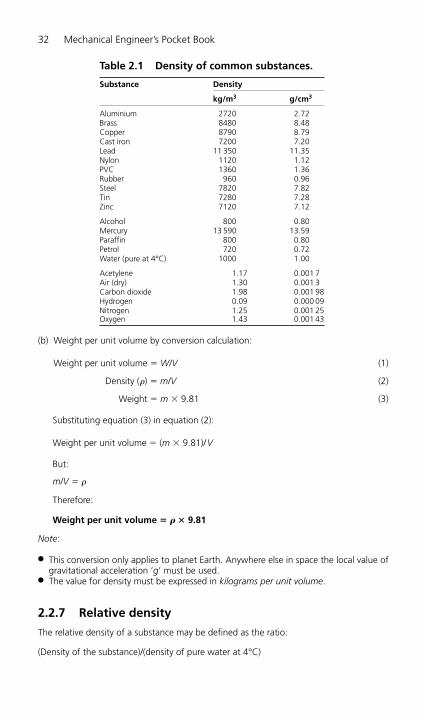
(b) Weight per unit volume by conversion calculation:
Weight per unit volume � W/V (1)
Density (�) � m/V (2)
Weight � m � 9.81 (3)
Substituting equation (3) in equation (2):
Weight per unit volume � (m � 9.81)/V
But:
m/V � �
Therefore:
Weight per unit volume � � � 9.81
Note:
● This conversion only applies to planet Earth. Anywhere else in space the local value ofgravitational acceleration ‘g’ must be used.
● The value for density must be expressed in kilograms per unit volume.
2.2.7 Relative density
The relative density of a substance may be defined as the ratio:
(Density of the substance)/(density of pure water at 4°C)
32 Mechanical Engineer’s Pocket Book
Table 2.1 Density of common substances.
Substance Density
kg/m3 g/cm3
Aluminium 2720 2.72Brass 8480 8.48Copper 8790 8.79Cast iron 7200 7.20Lead 11 350 11.35Nylon 1120 1.12PVC 1360 1.36Rubber 960 0.96Steel 7820 7.82Tin 7280 7.28Zinc 7120 7.12
Alcohol 800 0.80Mercury 13 590 13.59Paraffin 800 0.80Petrol 720 0.72Water (pure at 4°C) 1000 1.00
Acetylene 1.17 0.001 7Air (dry) 1.30 0.001 3Carbon dioxide 1.98 0.001 98Hydrogen 0.09 0.000 09Nitrogen 1.25 0.001 25Oxygen 1.43 0.001 43
H6508-Ch02.qxd 9/12/05 4:39 PM Page 32
or
(Mass of the substance)/(mass of an equal volume of pure water at 4°C)
Since relative density is a ratio there are no units.
The relative densities of some common substances used in engineering are given in Table 2.2.
Engineering Statics 33
Table 2.2 Relative densities of some commonsubstances.
Substance Relative density (d )
Aluminium 2.72Brass 8.48Cadmium 8.57Chromium 7.03Copper 8.79Cast iron 7.20Lead 11.35Nickel 8.73Nylon 1.12PVC 1.36Rubber 0.96Steel 7.82Tin 7.28Zinc 7.12
Alcohol 0.80Mercury 13.95Paraffin 0.80Petrol 0.72Water (pure @ 4°C) 1.00Water (sea) 1.02
Acetylene 0.001 7Air (dry) 0.001 3Carbon dioxide 0.001 98Carbon monoxide 0.001 26Hydrogen 0.000 09Nitrogen 0.001 25Oxygen 0.001 43
2.2.8 Pressure (fluids)
The pressure acting on the surface area of a body is defined as the normal force per unitarea acting on the surface. Normal force means the force acting at right angles to the sur-face. The SI unit of fluid pressure is the pascal (Pa), where 1 Pa is equal to 1 Nm2.
Pressure (p) � F/A
where:p � pressure in pascalsF � force in newtons acting at right angles (normal) to the surfaceA � area of the surface in metres squared
Similarly:
1 MPa � 1 MN/m2 � 1 N/mm2
H6508-Ch02.qxd 9/12/05 4:39 PM Page 33
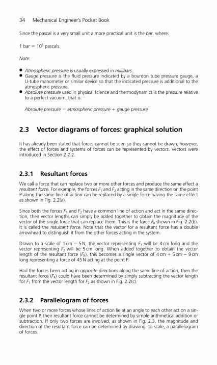
34 Mechanical Engineer’s Pocket Book
Since the pascal is a very small unit a more practical unit is the bar, where:
1 bar � 105 pascals.
Note:
● Atmospheric pressure is usually expressed in millibars.● Gauge pressure is the fluid pressure indicated by a bourdon tube pressure gauge, a
U-tube manometer or similar device so that the indicated pressure is additional to theatmospheric pressure.
● Absolute pressure used in physical science and thermodynamics is the pressure relativeto a perfect vacuum, that is:
Absolute pressure � atmospheric pressure � gauge pressure
2.3 Vector diagrams of forces: graphical solution
It has already been stated that forces cannot be seen so they cannot be drawn; however,the effect of forces and systems of forces can be represented by vectors. Vectors wereintroduced in Section 2.2.2.
2.3.1 Resultant forces
We call a force that can replace two or more other forces and produce the same effect aresultant force. For example, the forces F1 and F2 acting in the same direction on the pointP along the same line of action can be replaced by a single force having the same effectas shown in Fig. 2.2(a).
Since both the forces F1 and F2 have a common line of action and act in the same direc-tion, their vector lengths can simply be added together to obtain the magnitude of thevector of the single force that can replace them. This is the force FR shown in Fig. 2.2(b).It is called the resultant force. Note that the vector for a resultant force has a doublearrowhead to distinguish it from the other forces acting in the system.
Drawn to a scale of 1 cm � 5 N, the vector representing F1 will be 4 cm long and the vector representing F2 will be 5 cm long. When added together to obtain the vectorlength of the resultant force (FR), this becomes a single vector of 4 cm � 5 cm � 9 cmlong representing a force of 45 N acting at the point P.
Had the forces been acting in opposite directions along the same line of action, then theresultant force (FR) could have been determined by simply subtracting the vector lengthfor F1 from the vector length for F2 as shown in Fig. 2.2(c).
2.3.2 Parallelogram of forces
When two or more forces whose lines of action lie at an angle to each other act on a sin-gle point P, their resultant force cannot be determined by simple arithmetical addition orsubtraction. If only two forces are involved, as shown in Fig. 2.3, the magnitude anddirection of the resultant force can be determined by drawing, to scale, a parallelogramof forces.
H6508-Ch02.qxd 9/12/05 4:39 PM Page 34

Engineering Statics 35
P
P
P
9 cm
4 cm 5 cm
(a) Forces F1 and F2 acting on point P
(c) Resultant of forces F1 and F2 acting in opposing directions
(b) Resultant of forces F1 and F2
4 cm
F1 � 20 N
FR � 45 N
F2 � 25 N
F1 � 20 N
FR � 5 N
F2 � 25 N
5 cm
Scale: 1 cm � 5 N
Figure 2.2 Resultant forces.
F1 � 40 NF1 � 40 N
FR � 87 N
F2 � 50 N F2 � 50 N
60°
P
(a) (b)
P C
A B
a
Scale: 1 cm � 10 N
Figure 2.3 Parallelogram of forces.
H6508-Ch02.qxd 9/12/05 4:39 PM Page 35
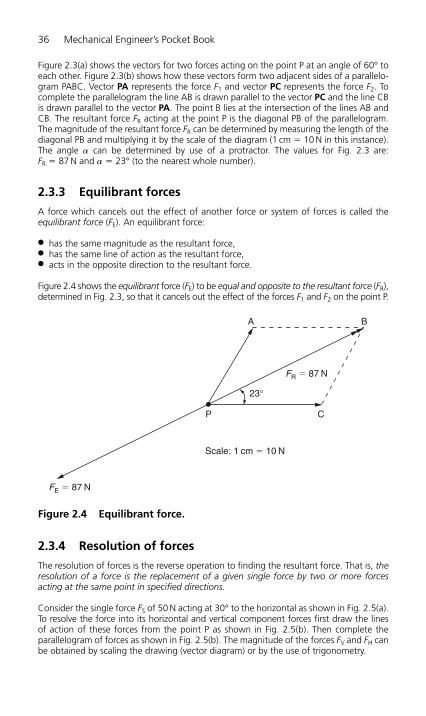
36 Mechanical Engineer’s Pocket Book
Figure 2.3(a) shows the vectors for two forces acting on the point P at an angle of 60° toeach other. Figure 2.3(b) shows how these vectors form two adjacent sides of a parallelo-gram PABC. Vector PA represents the force F1 and vector PC represents the force F2. Tocomplete the parallelogram the line AB is drawn parallel to the vector PC and the line CBis drawn parallel to the vector PA. The point B lies at the intersection of the lines AB andCB. The resultant force FR acting at the point P is the diagonal PB of the parallelogram.The magnitude of the resultant force FR can be determined by measuring the length of thediagonal PB and multiplying it by the scale of the diagram (1 cm � 10 N in this instance).The angle � can be determined by use of a protractor. The values for Fig. 2.3 are:FR � 87 N and � � 23° (to the nearest whole number).
2.3.3 Equilibrant forces
A force which cancels out the effect of another force or system of forces is called theequilibrant force (FE). An equilibrant force:
● has the same magnitude as the resultant force,● has the same line of action as the resultant force,● acts in the opposite direction to the resultant force.
Figure 2.4 shows the equilibrant force (FE) to be equal and opposite to the resultant force (FR),determined in Fig. 2.3, so that it cancels out the effect of the forces F1 and F2 on the point P.
A
P
FE � 87 N
C
B
FR � 87 N
23°
Scale: 1 cm � 10 N
Figure 2.4 Equilibrant force.
2.3.4 Resolution of forces
The resolution of forces is the reverse operation to finding the resultant force. That is, theresolution of a force is the replacement of a given single force by two or more forces acting at the same point in specified directions.
Consider the single force FS of 50 N acting at 30° to the horizontal as shown in Fig. 2.5(a).To resolve the force into its horizontal and vertical component forces first draw the lines of action of these forces from the point P as shown in Fig. 2.5(b). Then complete the parallelogram of forces as shown in Fig. 2.5(b). The magnitude of the forces FV and FH canbe obtained by scaling the drawing (vector diagram) or by the use of trigonometry.
H6508-Ch02.qxd 9/12/05 4:39 PM Page 36
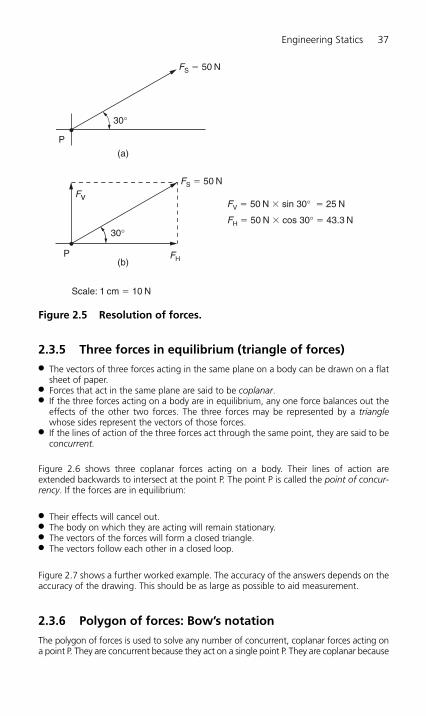
Engineering Statics 37
FS � 50 N
FS � 50 N
FV � 50 N � sin 30° � 25 N
FH � 50 N � cos 30° � 43.3 N
Fv
FH
30°
30°
P
P
(a)
(b)
Scale: 1 cm � 10 N
Figure 2.5 Resolution of forces.
2.3.5 Three forces in equilibrium (triangle of forces)● The vectors of three forces acting in the same plane on a body can be drawn on a flat
sheet of paper.● Forces that act in the same plane are said to be coplanar.● If the three forces acting on a body are in equilibrium, any one force balances out the
effects of the other two forces. The three forces may be represented by a trianglewhose sides represent the vectors of those forces.
● If the lines of action of the three forces act through the same point, they are said to beconcurrent.
Figure 2.6 shows three coplanar forces acting on a body. Their lines of action areextended backwards to intersect at the point P. The point P is called the point of concur-rency. If the forces are in equilibrium:
● Their effects will cancel out.● The body on which they are acting will remain stationary.● The vectors of the forces will form a closed triangle.● The vectors follow each other in a closed loop.
Figure 2.7 shows a further worked example. The accuracy of the answers depends on theaccuracy of the drawing. This should be as large as possible to aid measurement.
2.3.6 Polygon of forces: Bow’s notation
The polygon of forces is used to solve any number of concurrent, coplanar forces acting ona point P. They are concurrent because they act on a single point P. They are coplanar because
H6508-Ch02.qxd 9/12/05 4:39 PM Page 37

38 Mechanical Engineer’s Pocket Book
they lie in the same plane. Figure 2.8(a) shows a space diagram with the spaces between theforces designated by capital letters. The corresponding force diagram is shown in Fig. 2.8(b)with the forces labelled using lower case letters. This is known as Bow’s notation:
● The forces acting on point P should be represented by vectors whose length and anglesmust be drawn to scale as accurately as possible. The spaces between the forces are
F2 � 20 N
F2
F3
F1
F3 � 35 N
Space diagram
Force diagram
Scale: 1 cm � 5 N
F1 � 20 N
P
Figure 2.6 Triangle of forces.
60°
30°
Tie
Force in Tie� 20 kN
Force in Jib� 34.6 kN
Force diagram
Space diagram Scale: 1 cm � 5 kN
Jib
Load20 kN
Load20 kN
Figure 2.7 Forces in a simple jib crane.
H6508-Ch02.qxd 9/12/05 4:39 PM Page 38
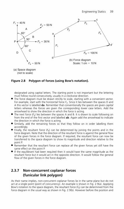
Engineering Statics 39
F1 � 40 N
d�
F2
F1
a
b c
d
F3
F4
F2 � 50 N
FR � 100 N
F3 � 30 N
F4 � 50 N
A
B
CD
(a) Space diagram (not to scale)
(b) Force diagram Scale: 1 cm � 10 N
P
60°
60°
30°
Figure 2.8 Polygon of forces (using Bow’s notation).
designated using capital letters. The starting point is not important but the letteringmust follow round consecutively, usually in a clockwise direction.
● The force diagram must be drawn strictly to scale, starting with a convenient vector.For example, start with the horizontal force F3. Since it lies between the spaces D andA this vector is labelled da. Remember that conventionally the spaces are given capitalletters whereas the forces are given the corresponding lower case letters. Add thearrowhead to show the direction in which the force is acting.
● The next force (F4) lies between the spaces A and B. It is drawn to scale following onfrom the end of the first vector and labelled ab. Again add the arrowhead to indicatethe direction in which the force is acting.
● Similarly, add the remaining forces so that they follow on in order labelling themaccordingly.
● Finally, the resultant force (FR) can be determined by joining the points and in the force diagram. Note that the direction of the resultant force is against the general flowof the given forces in the force diagram. If required, the resultant force can now betransferred to the space diagram to show its magnitude and direction relative to thepoint P.
● Remember that the resultant force can replace all the given forces yet still have thesame effect on the point P.
● If the equilibrant had been required then it would have the same magnitude as theresultant force but it would act in the opposite direction. It would follow the generalflow of the given forces in the force diagram.
2.3.7 Non-concurrent coplanar forces (funicular link polygon)
As their name implies, non-concurrent coplanar forces lie in the same plane but do notact at a single point (point of concurrency). An example is shown in Fig. 2.9(a). ApplyingBow’s notation to the space diagram, the resultant force (FR) can be determined from theforce diagram in the usual way as shown in Fig. 2.9(b). However before the position and
H6508-Ch02.qxd 9/12/05 4:39 PM Page 39
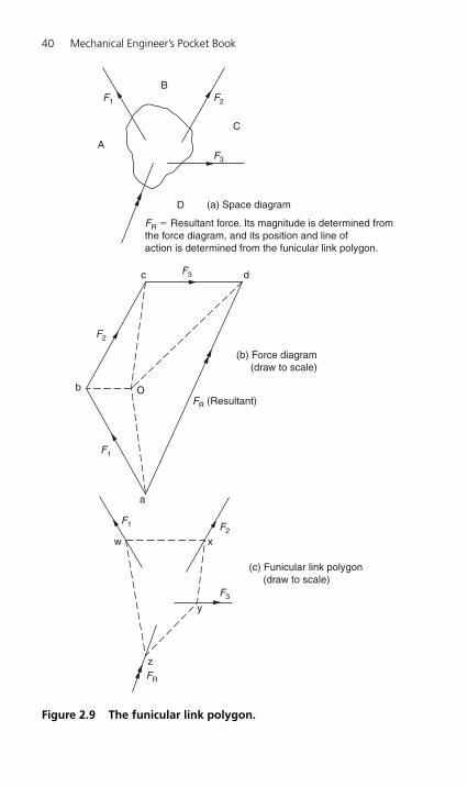
40 Mechanical Engineer’s Pocket Book
B
C
D
A
F1 F2
F3
(a) Space diagram
(b) Force diagram (draw to scale)
(c) Funicular link polygon (draw to scale)
FR � Resultant force. Its magnitude is determined fromthe force diagram, and its position and line ofaction is determined from the funicular link polygon.
F3
FR (Resultant)
F2
F1
F1 F2
FR
F3
x
y
z
w
dc
b
a
O
Figure 2.9 The funicular link polygon.
H6508-Ch02.qxd 9/12/05 4:39 PM Page 40
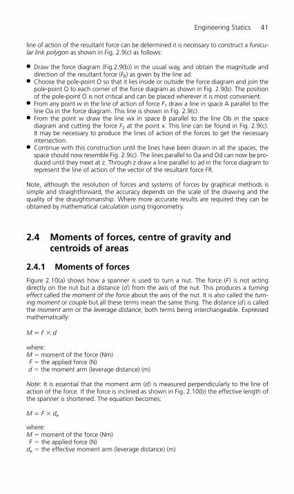
Engineering Statics 41
line of action of the resultant force can be determined it is necessary to construct a funicu-lar link polygon as shown in Fig. 2.9(c) as follows:
● Draw the force diagram (Fig.2.9(b)) in the usual way, and obtain the magnitude anddirection of the resultant force (FR) as given by the line ad.
● Choose the pole-point O so that it lies inside or outside the force diagram and join thepole-point O to each corner of the force diagram as shown in Fig. 2.9(b). The positionof the pole-point O is not critical and can be placed wherever it is most convenient.
● From any point w in the line of action of force F1 draw a line in space A parallel to theline Oa in the force diagram. This line is shown in Fig. 2.9(c).
● From the point w draw the line wx in space B parallel to the line Ob in the space diagram and cutting the force F2 at the point x. This line can be found in Fig. 2.9(c). It may be necessary to produce the lines of action of the forces to get the necessaryintersection.
● Continue with this construction until the lines have been drawn in all the spaces, thespace should now resemble Fig. 2.9(c). The lines parallel to Oa and Od can now be pro-duced until they meet at z. Through z draw a line parallel to ad in the force diagram torepresent the line of action of the vector of the resultant force FR.
Note, although the resolution of forces and systems of forces by graphical methods is simple and straightforward, the accuracy depends on the scale of the drawing and thequality of the draughtsmanship. Where more accurate results are required they can beobtained by mathematical calculation using trigonometry.
2.4 Moments of forces, centre of gravity and centroids of areas
2.4.1 Moments of forces
Figure 2.10(a) shows how a spanner is used to turn a nut. The force (F) is not actingdirectly on the nut but a distance (d ) from the axis of the nut. This produces a turningeffect called the moment of the force about the axis of the nut. It is also called the turn-ing moment or couple but all these terms mean the same thing. The distance (d ) is calledthe moment arm or the leverage distance, both terms being interchangeable. Expressedmathematically:
M � F � d
where:M � moment of the force (Nm)F � the applied force (N)d � the moment arm (leverage distance) (m)
Note: It is essential that the moment arm (d) is measured perpendicularly to the line ofaction of the force. If the force is inclined as shown in Fig. 2.10(b) the effective length ofthe spanner is shortened. The equation becomes:
M � F � de
where:M � moment of the force (Nm)F � the applied force (N)
de � the effective moment arm (leverage distance) (m)
H6508-Ch02.qxd 9/12/05 4:39 PM Page 41
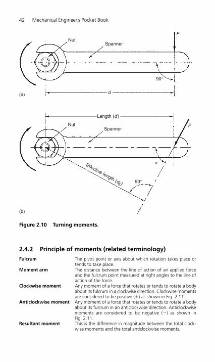
42 Mechanical Engineer’s Pocket Book
2.4.2 Principle of moments (related terminology)
Fulcrum The pivot point or axis about which rotation takes place ortends to take place.
Moment arm The distance between the line of action of an applied forceand the fulcrum point measured at right angles to the line ofaction of the force.
Clockwise moment Any moment of a force that rotates or tends to rotate a bodyabout its fulcrum in a clockwise direction. Clockwise momentsare considered to be positive (�) as shown in Fig. 2.11.
Anticlockwise moment Any moment of a force that rotates or tends to rotate a bodyabout its fulcrum in an anticlockwise direction. Anticlockwisemoments are considered to be negative (�) as shown in Fig. 2.11.
Resultant moment This is the difference in magnitude between the total clock-wise moments and the total anticlockwise moments.
(b)
FSpanner
90°
aEffective length (dE )
Nut
(a)
NutSpanner
90°
F
d
Length (d )
Figure 2.10 Turning moments.
H6508-Ch02.qxd 9/12/05 4:39 PM Page 42

Engineering Statics 43
Anticlockwise(�)
Clockwise(�)
Fulcrum
Figure 2.11 Clockwise and anticlockwise moments.
2.4.3 Principle of moments
The algebraic sum of the moments of a number of forces acting about anypoint is equal to the resultant moment of force about the same point.
Expressed mathematically:
MR � M1 � M2 � (�M3) � … � Mn
where:MR � the resultant moment of force
M1 to Mn � any number of moments acting about the same fulcrum point
Remember: The positive moments will be acting in a clockwise direction, whereas thenegative moments (such as �M3) will be acting in an anticlockwise direction.
2 m
(a)
(b)
F1 � 25 N
FR � 15 N
Fulcrum
F2 � 40 N
F2 � 50 N
2 m
2 m
3 m
Figure 2.12 Application of principle of moments.
H6508-Ch02.qxd 9/12/05 4:39 PM Page 43

Applying the above principles to the lever in Fig. 2.12(a), calculate:
(a) The magnitude of the resultant force.(b) The magnitude of the resultant moment.(c) The position of the line of action of the resultant force.
(a) Since the lines of action of the applied forces acting on the lever shown in Fig. 2.12(a)are parallel to each other, the resultant force (FR) can be obtained by simple additionand subtraction:● Forces F1 and F2 tend to move the lever upwards. They are acting in the same direc-
tion, therefore they can be added together.● Force F3 acts in the opposite direction, therefore it is subtracted from the sum of
F1 and F2.
Therefore:
FR � F1 � F2 � F3
� 25 N � 40 N � 50 N
� 15 N
(b) To find the magnitude of the resultant moment (MR)
Clockwise moments (�):
M1 � F1 � (2 m � 2 m) � 25 N � 4 m � 100 Nm
M2 � F2 � 2 m � 40 N � 2 m � 80 Nm
Anticlockwise moments (�):
M3 � F3 � 3 m � 50 N � 3 m � 150 Nm
Resultant moment:
MR � M1 � M2 � M3 � 100 Nm � 80 Nm � 150 Nm
� 30 Nm
(c) To combine the results of (a) and (b) in order to find the position of the line of actionof the resultant force (FR), refer to Fig. 2.12(b).
MR � FR � d � 30 Nm
Therefore:
30 Nm � 15 N � d
d � 30 Nm/15 N � 2 m
Therefore the forces F1, F2 and F3 can be replaced by the single force FR acting at a point2 m from the fulcrum. Since MR is positive the force FR will move or tend to move the leverin a clockwise direction so the force FR will act in an upwards direction as shown.
44 Mechanical Engineer’s Pocket Book
H6508-Ch02.qxd 9/12/05 4:39 PM Page 44

Engineering Statics 45
2.4.4 Equilibrium
In the previous section, the moments have not acted in equal and opposite directions.This has resulted in a residual, resultant force, causing or tending to cause a rotationabout a pivot point (fulcrum).
Figure 2.13 shows a simple balance scale in which the masses M1 and M2 in the scale pansare of equal magnitude so that the scales balance and the beam is horizontal. Since theforce of gravity acts equally on M1 and M2, the forces F1 and F2 are also equal. The reac-tion force (R) equals the sum of the downward forces.
F1 F2
M2M1
FR
Figure 2.13 Simple balance scale.
The forces are equidistant from the fulcrum, so the turning moments are also equal. Sincethe turning moments act in opposite directions these moments are also in equilibrium.They balance each other and there is no tendency for the scale-beam to rotate. This canbe summarized as follows:
When a body is in a state of equilibrium (balance) under the action of anumber of forces, the clockwise moments about any point is equal to theanticlockwise moments about the same point.
Put more elegantly:
The algebraic sum of the moments about any point is zero.
For a body to be in a state of equilibrium the following conditions must exist:
● The algebraic sum of the horizontal forces acting on the body must equal zero,�FH � 0.
● The algebraic sum of the vertical forces acting on the body must equal zero, �FV � 0.● The algebraic sum of the moments acting on the body must equal zero, �M � 0.
Figure 2.14 shows a lever pivoted at its centre. The line of action of a force F1 is 2 m to theleft of the pivot and tends to impart an anticlockwise moment. The line of action of forceF2 is 3 m to the right of the pivot and tends to impart a clockwise moment. If the magni-tude of F2 is 20 N, calculate:
1. The magnitude of the force F1 required to put the lever into a state of equilibrium.2. The magnitude of the reaction force (FR) at the pivot.
H6508-Ch02.qxd 9/12/05 4:39 PM Page 45

46 Mechanical Engineer’s Pocket Book
2 m
F1 F2 � 20 N
FR
3 m
Figure 2.14 Forces in equilibrium.
For equilibrium:
Clockwise moments � anticlockwise moments(20 N � 3 m) � (F1 � 2 m)
F1 � (20 N � 3 m)/2 m � 30 N
The reaction force FR, acting upwards, is equal and opposite to the sum of F1 and F2 act-ing downwards. Therefore:
R � F1 � F2 � 20 N � 30 N � 50 N
Figure 2.15 shows a simple beam supported at each end. Since it is in equilibrium there isno tendency for it to rotate and the reaction forces RA and RB at the supports can be cal-culated using the principle of moments. This is achieved by taking moments about eachsupport in turn.
600 N
RA RB
3 m 3 m4 m
500 N
Figure 2.15 Calculation of reaction forces.
To determine the magnitude of RA take moments about RB in order to eliminate it fromthe initial calculation so that only one unknown quantity has to be calculated as follows:
Clockwise moments � anticlockwise momentsRA � 10 m � (600 N � 7 m) � (500 N � 3 m)
RA � 10 m � 4200 Nm � 1500 Nm
RA � 10 m � 5700 Nm
RA � 5700 Nm/10 m
RA � 570 N
H6508-Ch02.qxd 9/12/05 4:39 PM Page 46

Similarly to determine the magnitude of RB take moments about RA in order to eliminate itfrom the initial calculation so that only one unknown quantity has to be calculated as follows:
Clockwise moments � anticlockwise moments
(600 N � 3 m) � (500 N � 7 m) � RB � 10 m
1800 Nm � 3500 Nm � RB � 10 m
5300 Nm � RB � 10 m
RB � 5300 Nm/10 m
RB � 530 N
For a system of forces in equilibrium the downward forces must equal the upward forces.
Therefore:
RA � RB � 600 N � 500 N
570 N � 530 N � 600 N � 500 N
1100 N � 1100 N
which is true. Therefore the calculation for RA and RB are correct. Avoid taking the short-cut of calculating on one of the reaction forces and deducting it from the sum of thedownward forces. Any error in the initial calculation will be carried forward and no checkwill be possible.
The above examples ignore the weight of the beam.
The weight of a uniform beam may be considered to be a concentrated forcewhose line of action can be assumed to act through the centre of the length ofthe beam.
2.5 Orders of levers
Figure 2.16 shows the three orders of levers. Applying the principle of moments, the rela-tionship between the load (W ), the distance of the load from the fulcrum (d1) and effort(F ), and the distance of the effort from the fulcrum (d2) is common to all the orders andcan be expressed mathematically as:
W � d1 � F � d2
Therefore:
W � F � d2/d1
And:
F � W � d1/d2
2.5.1 First-order levers● The fulcrum is positioned between the effort and the load.● The effort force is smaller than the load.● The effort moves further than the load.● This order of levers can be considered as a force magnifier.
Engineering Statics 47
H6508-Ch02.qxd 9/12/05 4:39 PM Page 47
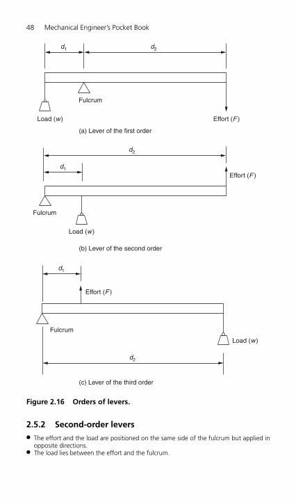
48 Mechanical Engineer’s Pocket Book
2.5.2 Second-order levers● The effort and the load are positioned on the same side of the fulcrum but applied in
opposite directions.● The load lies between the effort and the fulcrum.
Fulcrum
d1 d2
(a) Lever of the first order
Fulcrum
d1
d2
Load (w )
Load (w )
(b) Lever of the second order
Fulcrum
Load (w)
d1
d2
Effort (F )
Effort (F )
Effort (F )
(c) Lever of the third order
Figure 2.16 Orders of levers.
H6508-Ch02.qxd 9/12/05 4:39 PM Page 48
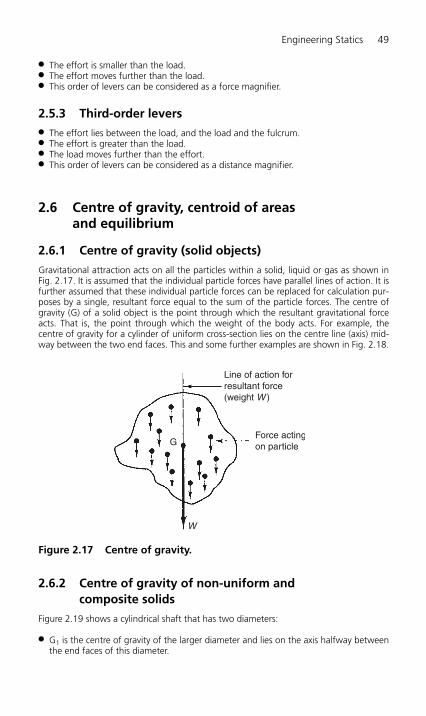
Engineering Statics 49
● The effort is smaller than the load.● The effort moves further than the load.● This order of levers can be considered as a force magnifier.
2.5.3 Third-order levers● The effort lies between the load, and the load and the fulcrum.● The effort is greater than the load.● The load moves further than the effort.● This order of levers can be considered as a distance magnifier.
2.6 Centre of gravity, centroid of areas and equilibrium
2.6.1 Centre of gravity (solid objects)
Gravitational attraction acts on all the particles within a solid, liquid or gas as shown inFig. 2.17. It is assumed that the individual particle forces have parallel lines of action. It isfurther assumed that these individual particle forces can be replaced for calculation pur-poses by a single, resultant force equal to the sum of the particle forces. The centre ofgravity (G) of a solid object is the point through which the resultant gravitational forceacts. That is, the point through which the weight of the body acts. For example, thecentre of gravity for a cylinder of uniform cross-section lies on the centre line (axis) mid-way between the two end faces. This and some further examples are shown in Fig. 2.18.
Line of action forresultant force(weight W )
Force actingon particleG
W
Figure 2.17 Centre of gravity.
2.6.2 Centre of gravity of non-uniform and composite solids
Figure 2.19 shows a cylindrical shaft that has two diameters:
● G1 is the centre of gravity of the larger diameter and lies on the axis halfway betweenthe end faces of this diameter.
H6508-Ch02.qxd 9/12/05 4:39 PM Page 49
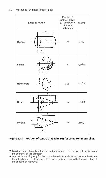
50 Mechanical Engineer’s Pocket Book
● G2 is the centre of gravity of the smaller diameter and lies on the axis halfway betweenthe end faces of this diameter.
● G is the centre of gravity for the composite solid as a whole and lies at a distance dfrom the datum end of the shaft. Its position can be determined by the application ofthe principal of moments.
Shape of volume
Position ofcentre of gravity(G) at distance
x from theend shown
Volume
h
h
h
h /2
h /4
h /4 abh /3
πr 2h
4πr 3/3
2πr 3/3
πr 2h /3
3r /8
r
r
x
x
x
x
x
b
r
r
ra
G
G
G
G
G
Cylinder
Sphere
Hemisphere
Cone
Pyramid
Figure 2.18 Position of centre of gravity (G) for some common solids.
H6508-Ch02.qxd 9/12/05 4:39 PM Page 50

Engineering Statics 51
1. The overall weight of the shaft is the sum of the weights of the two cylinders. That is,10 kN � 5 kN � 15 kN.
2. The total weight of 15 kN will act through the centre of gravity G for the shaft as awhole at some distance d from the datum point P about which moments are taken.
3. For this calculation it is conventionally assumed that the moment of G about the pointP will be the opposite hand to the moments of G1 and G2 about P, despite the fact thatthey all appear to produce clockwise moments.
Clockwise moments � anticlockwise moments
(G1 � 1 m) � (G2 � 4 m) � (G � d)
(10 kN � 1 m) � (5 kN � 3 m) � (15 kN � d)
10 kN m � 15 kN m � 15 kN � d
25 kN m � 15 kN � d
Therefore:
d � 25 kN m/15 kN � 1.67 m
The same technique can be used for composite solids where the densities of the variouselements differ.
2.6.3 Centre of gravity (lamina)
For a thin sheet metal or rigid sheet plastic component of uniform thickness (a lamina)where the thickness is negligible compared with its area, the centre of gravity can be
2.0 m
1.0 m
3 m
10 kNd
G1 G2G
(10 � 5) kN 5 kN
2.0 m
Figure 2.19 To determine the centre of gravity for a non-uniform solid.
H6508-Ch02.qxd 9/12/05 4:39 PM Page 51
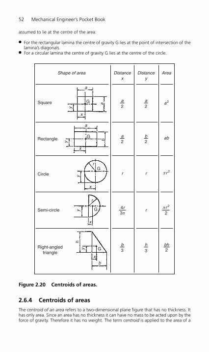
52 Mechanical Engineer’s Pocket Book
assumed to lie at the centre of the area:
● For the rectangular lamina the centre of gravity G lies at the point of intersection of thelamina’s diagonals.
● For a circular lamina the centre of gravity G lies at the centre of the circle.
Shape of area
Square
Rectangle
Circle
Semi-circle
Right-angledtriangle
G
G
G
G
G
ab
a
a
r
r
r r
r
a2
πr 2
x
x
x
x
xb
ab
yy
yy
yh
Distancex
Distancey
Area
a2
a2
b3
h3
bh2
4r3π
πr 2
2
b2
a2
Figure 2.20 Centroids of areas.
2.6.4 Centroids of areas
The centroid of an area refers to a two-dimensional plane figure that has no thickness. Ithas only area. Since an area has no thickness it can have no mass to be acted upon by theforce of gravity. Therefore it has no weight. The term centroid is applied to the area of a
H6508-Ch02.qxd 9/12/05 4:39 PM Page 52

two-dimensional plane figure in much the way that centre of gravity is applied to a solidlamina. Therefore the centroid of an area is the point on a plane figure where the wholearea is considered to be concentrated. Like the centre of gravity, the centroid of an areais also denoted by the letter G. Some examples of centroids are shown in Fig. 2.20.
2.6.5 Equilibrium
Equilibrium was introduced in Section 2.4.4. Consider Fig. 2.21(a) which shows a bar ofmetal of uniform section pivoted at its centre so that it is free to rotate. Figure 2.21(a) alsoshows that the turning moments acting on each arm of the bar, due to force of gravity,are equal and opposite. Therefore, being perfectly balanced the bar should remain in anyposition to which it is turned. The bar is said to be in a state of neutral equilibrium.
In Fig. 2.21(b) the same bar is shown pivoted off-centre so that one arm is longer than theother. With the bar upright as shown in Fig. 2.21(b), the line of action of the vector
Engineering Statics 53
M1
d1
o oP
Pivot
d2
d1 � d2
M1 � M2
M2
G
(a) Neutral or stable equilibrium
o
o
o
GG
P
o
(b) Unstable equilibrium
Figure 2.21 Equilibrium.
H6508-Ch02.qxd 9/12/05 4:39 PM Page 53
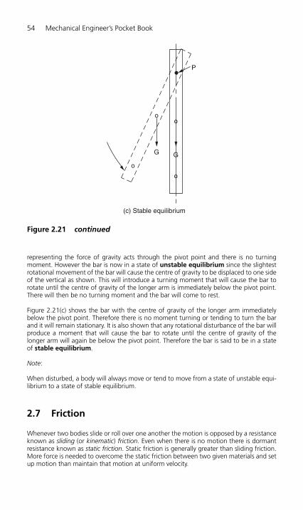
54 Mechanical Engineer’s Pocket Book
representing the force of gravity acts through the pivot point and there is no turningmoment. However the bar is now in a state of unstable equilibrium since the slightestrotational movement of the bar will cause the centre of gravity to be displaced to one sideof the vertical as shown. This will introduce a turning moment that will cause the bar torotate until the centre of gravity of the longer arm is immediately below the pivot point.There will then be no turning moment and the bar will come to rest.
Figure 2.21(c) shows the bar with the centre of gravity of the longer arm immediatelybelow the pivot point. Therefore there is no moment turning or tending to turn the barand it will remain stationary. It is also shown that any rotational disturbance of the bar willproduce a moment that will cause the bar to rotate until the centre of gravity of thelonger arm will again be below the pivot point. Therefore the bar is said to be in a stateof stable equilibrium.
Note:
When disturbed, a body will always move or tend to move from a state of unstable equi-librium to a state of stable equilibrium.
2.7 Friction
Whenever two bodies slide or roll over one another the motion is opposed by a resistanceknown as sliding (or kinematic) friction. Even when there is no motion there is dormantresistance known as static friction. Static friction is generally greater than sliding friction.More force is needed to overcome the static friction between two given materials and setup motion than maintain that motion at uniform velocity.
o
o
o
o
GG
(c) Stable equilibrium
P
Figure 2.21 continued
H6508-Ch02.qxd 9/12/05 4:39 PM Page 54
2.7.1 Lubrication
Friction and wear between sliding or rolling surfaces can be greatly reduced if the surfacesof the materials are separated by a suitable film of lubricant. Oils are generally used tolubricate rapidly moving surfaces subject to relatively light loads and greases are generallyused to lubricate slow moving surfaces subject to heavier loads. If separation of the sur-faces is complete, dry friction is eliminated and there is only the fluid friction or viscosityof the oil which has to be overcome. As well as reducing wear and friction, lubricationalso serves to protect the sliding surfaces against corrosion and reduce the generation ofheat which represents wasted energy. Any heat that is generated tends to be dissipatedby the lubricant.
2.7.2 Laws of friction
The amount of friction between two surfaces sliding or rolling over one another is gov-erned by the following factors:
● The surface texture of the surfaces involved. Smoothness reduces friction; roughnessincreases friction.
● The kind of materials in contact (e.g. steel slides more easily on nylon than it does onrubber).
● The magnitude of the normal (at right angles) reaction forces between the surfaces.● Friction is independent of area.
2.7.3 Coefficient of friction
The coefficient of friction (symbol �) for a pair of surfaces in contact is given by theexpression:
� � (friction force Ff)/(the normal reaction force Fn)
This is shown in Fig. 2.22. Since Ff and Fn are both expressed in the same units, � is ratioand has no units.
Engineering Statics 55
Weight (W )
Frictionforce (Ff)
Normal reaction force (Fn)
Appliedforce (Fa)
Figure 2.22 Friction.
Case 1A block of weight W is pulled along a horizontal surface by an applied force of magnitudeFa as shown in Fig. 2.22. Whilst the block moves at a uniform speed or while it is stationary,
H6508-Ch02.qxd 9/12/05 4:39 PM Page 55
56 Mechanical Engineer’s Pocket Book
a resistance is experienced that is equal and opposite to the applied force Fa. This resistanceis the friction force Ff. This friction force always opposes motion. Thus, in this case:
� � Ff /Fn � Fa/W
● If the friction force equals the applied force the block is stationary or in a state of uni-form motion and the forces acting on it are in equilibrium.
● If the block tends to accelerate then the applied force is greater than the friction force.● The friction force can be less than or equal to the applied force. It can never be greater
than the applied force. That is, Ff is equal to or less than Fa, and Fn is equal to or lessthan W.
Case 2If the applied force (Fa) is inclined at an angle � to the sliding block as shown in Fig. 2.23then the friction force Ff will be equal and opposite to the horizontal component force(Fh), where Fh � Fa cos �. The vertical component force Fv � Fa sin �. And this force isopposing the weight W and, hence, reducing the normal reaction force, Fn. Therefore:
� � Ff /Fn � (Fa cos �)/(W � Fa sin �)
Weight (W )
Frictionforce (Ff)
Fn
Horizontal component force Fh � (Fa cos u)
Vertical componentforce Fv � (Fa sin u)u
Appliedforce (Fa)
Figure 2.23 Friction – applied force inclined.
Thus if the applied force Fa acted downwards towards the horizontal surface, then Fh thenormal reaction force Fn will be increased. Therefore in this instance:
� � Ff /Fn � (Fa cos �)/(W � Fa sin �)
Table 2.3 gives some typical values of the coefficient of friction for various combinationsof sliding surfaces.
Table 2.3 Typical values for coefficients of friction.
Materials (dry) ��
Steel on cast iron 0.20Steel on brass 0.15Cast iron on brass 0.15Leather on cast iron 0.55Brake lining on cast iron 0.60Rubber on asphalt 0.65Rubber on concrete 0.70
H6508-Ch02.qxd 9/12/05 4:39 PM Page 56
Since Ff and Fn are at right angles:
tan � � Ff /Fn
but � � Ff /Fn
therefore:
tan � � �
The angle � reaches a maximum value when Ff is a maximum. This maximum value of � is known as the angle of friction.
2.7.5 Friction on an inclined plane
To determine the applied force Fa to pull a body of weight W up a plane inclined at anangle � to the horizontal when Fa is acting in at an angle � to the inclined plane as shownin Fig. 2.25.
Force Fa is acting at angle � to the plane, as shown in Fig. 2.25, and the normal reactionbetween the plane and the body is Fn. Resolving the forces perpendicular to the inclined plane:
Fn � Fa sin � � W cos �
Fn � W cos � � Fa sin �
The frictional force opposing the motion of the body is:
Ff � �Fn
� �(W cos � � Fa sin �) (1)
Engineering Statics 57
Fr
Fn
Ff
φ
Figure 2.24 Angle of friction.
2.7.4 Angle of friction
The forces Ff and Fn may be added vectorially as shown in Fig. 2.24 to give the resultantreaction Fr at the surface, since they are both exerted on the sliding block which is in con-tact with the horizontal surface.
H6508-Ch02.qxd 9/12/05 4:39 PM Page 57
58 Mechanical Engineer’s Pocket Book
Fa
Fa � Applied force
Fn � Normal (reaction) force
Ff � Friction (reaction) force
W � Weight of body
µ � Coefficient of frictionFnFf
W
u
φ
Figure 2.25 Friction on an inclined plane.
Resolving the forces parallel to the inclined plane:
Fa cos � � Ff � W sin �
Substituting for Ff from equation (1) gives:
Fa cos � � �(W cos � � Fa sin �) � W sin �
Fa cos � � W(� cos � � sin �) � �Fa sin �
Fa(� sin � � cos �) � W(� cos � � sin �)
Fa � [W(� cos � � sin �)]/[(� sin � � cos �)] (2)
(i) When Fa is applied parallel to the plane, then � � 0. Hence sin � � 0 and cos � � 1.Substituting in equation (2):
Fa � [W(� cos � � sin � )]/(1 � 0)
Fa � W(� cos U � sin U)
(ii) When Fa is applied horizontally, then it assists the motion of the body up the plane,then � � ��. Hence:
cos � � cos(�� ) � cos � and
sin � � sin(��) � �sin �
Substituting in equation (2):
Fa � W(� cos � � sin �)/(cos � � sin �)
2.7.6 Angle of repose
A body resting on a rough plane inclined at an angle � to the horizontal as shown in Fig. 2.26 is in a state of equilibrium when the gravitational force tending to slide the body
H6508-Ch02.qxd 9/12/05 4:40 PM Page 58
Engineering Statics 59
W
W cos u
W sin u
Ff
Fn
u
u
Figure 2.26 Angle of repose.
down the inclined plane is balanced by an equal and opposite frictional force acting upthe inclined plane. The angle of inclination of the inclined plane at which the equilibriumconditions apply is called the angle of repose.
The gravitational force acting on the body (W ) can be resolved into its component forcessuch that the component force acting perpendicularly to the inclined plane will be W cos �and the component force acting parallel to the inclined plane will be W sin �. For equilib-rium when the body is just about to slide down the inclined plane:
� � Ff /Fn � (W sin �)/(W cos �) � tan ��
From Section 2.7.4 the angle of friction, � � tan �; therefore for the body to be in a stateof repose, � � �. If � � � the body will slide down the inclined plane. If angle � � � thebody will remain at rest unless an external force is applied to cause motion.
2.8 Stress and strain
2.8.1 Direct stress
Figure 2.27(a) shows a cylindrical bar of cross-sectional area A in tension, whilst Fig. 2.27(b) shows the same bar in compression. The applied forces F are in line and arenormal (perpendicular) to the cross-sectional area of the bar. Therefore the bar is said tobe subject to direct stress. Direct stress is given the symbol � (Greek letter sigma).
Direct stress � � applied force F/cross-sectional area A
H6508-Ch02.qxd 9/12/05 4:40 PM Page 59

60 Mechanical Engineer’s Pocket Book
A
F F
A
F F
(a) Bar in tension – tensile stress
(b) Bar in compression – compressive stress
Figure 2.27 Direct stress.
2.8.2 Shear stress
Figure 2.28 shows a riveted joint. Since the applied forces Q are offset (not in line) the rivet is said to be subjected to shear stress which is given the symbol � (Greek letter tau).
Shear stress � � shear force Q/area in shear A
Direct stress and shear stress are usually of sufficient magnitude to be measured inMN/m2.
Q
Rivet
Q
Figure 2.28 Shear (indirect) stress.
H6508-Ch02.qxd 9/12/05 4:40 PM Page 60
2.8.3 Direct strain
The forces acting on a body that produce direct stress also cause a change in the dimen-sions of that body. For example, a tensile load will produce tensile stress and also cause thebody to stretch as shown in Fig. 2.29(a). Similarly, a compressive load causes the body toshorten as shown in Fig. 2.29(b). Direct strain is given the symbol (Greek letter epsilon).
Direct strain � change in length xloriginal length l
Since both the change in length and the original length are measured in the same units,strain is a ratio and has no units.
Engineering Statics 61
F
F
l
F
x
F
l
x
(a) Direct strain resulting from tensile stress
(b) Direct strain resulting from compressive stress
Figure 2.29 Direct strain.
2.8.4 Shear strain
Shear strain is shown in Fig. 2.30. The applied forces Q are offset and cause material todeform. Shear strain is given the symbol (Greek letter gamma).
Shear strain � deformation x/original dimension l
Again this is a ratio so there are no units.
2.8.5 Modulus of elasticity (Hooke’s law)
Hooke’s law states that within the elastic range for any given material, the deformation isproportional to the applied force producing it. When this law is applied to a spring:
Stiffness of the spring � direct stress �/direct strain
The modulus of elasticity E can be derived from Hooke’s law. Stress is directly proportionalto strain whilst the material is stressed within its elastic range, thus:
Stress strain
H6508-Ch02.qxd 9/12/05 4:40 PM Page 61
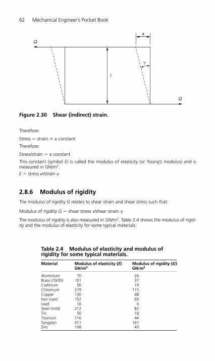
62 Mechanical Engineer’s Pocket Book
Therefore:
Stress � strain � a constant
Therefore:
Stress/strain � a constant
This constant (symbol E) is called the modulus of elasticity (or Young’s modulus) and ismeasured in GN/m2.E � stress �/strain
2.8.6 Modulus of rigidity
The modulus of rigidity G relates to shear strain and shear stress such that:
Modulus of rigidity G � shear stress �/shear strain
The modulus of rigidity is also measured in GN/m2. Table 2.4 shows the modulus of rigid-ity and the modulus of elasticity for some typical materials.
l
x
Q
Q
�
Figure 2.30 Shear (indirect) strain.
Table 2.4 Modulus of elasticity and modulus ofrigidity for some typical materials.
Material Modulus of elasticity (E) Modulus of rigidity (G)GN/m2 GN/m2
Aluminium 70 26Brass (70/30) 101 37Cadmium 50 19Chromium 279 115Copper 130 48Iron (cast) 152 60Lead 16 6Steel (mild) 212 82Tin 50 18Titanium 116 44Tungsten 411 161Zinc 108 43
H6508-Ch02.qxd 9/12/05 4:40 PM Page 62
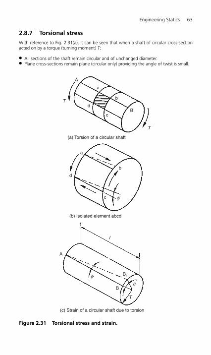
2.8.7 Torsional stress
With reference to Fig. 2.31(a), it can be seen that when a shaft of circular cross-sectionacted on by a torque (turning moment) T:
● All sections of the shaft remain circular and of unchanged diameter.● Plane cross-sections remain plane (circular only) providing the angle of twist is small.
Engineering Statics 63
(a) Torsion of a circular shaft
A
a
d
b
Bc
T
T
(b) Isolated element abcd
a
b
c
d
φ
(c) Strain of a circular shaft due to torsion
A
B
B1
l
T
φ
θ
Figure 2.31 Torsional stress and strain.
H6508-Ch02.qxd 9/12/05 4:40 PM Page 63
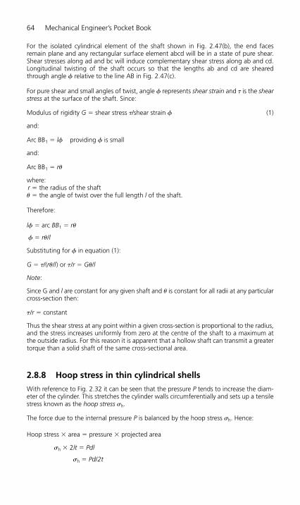
For the isolated cylindrical element of the shaft shown in Fig. 2.47(b), the end facesremain plane and any rectangular surface element abcd will be in a state of pure shear.Shear stresses along ad and bc will induce complementary shear stress along ab and cd.Longitudinal twisting of the shaft occurs so that the lengths ab and cd are shearedthrough angle � relative to the line AB in Fig. 2.47(c).
For pure shear and small angles of twist, angle � represents shear strain and � is the shearstress at the surface of the shaft. Since:
Modulus of rigidity G � shear stress �/shear strain � (1)
and:
Arc BB1 � l� providing � is small
and:
Arc BB1 � r�
where:r � the radius of the shaft� � the angle of twist over the full length l of the shaft.
Therefore:
l� � arc BB1 � r�
� � r�/l
Substituting for � in equation (1):
G � �/(r�/l) or �/r � G�/l
Note:
Since G and l are constant for any given shaft and � is constant for all radii at any particularcross-section then:
�/r � constant
Thus the shear stress at any point within a given cross-section is proportional to the radius,and the stress increases uniformly from zero at the centre of the shaft to a maximum atthe outside radius. For this reason it is apparent that a hollow shaft can transmit a greatertorque than a solid shaft of the same cross-sectional area.
2.8.8 Hoop stress in thin cylindrical shells
With reference to Fig. 2.32 it can be seen that the pressure P tends to increase the diam-eter of the cylinder. This stretches the cylinder walls circumferentially and sets up a tensilestress known as the hoop stress �h.
The force due to the internal pressure P is balanced by the hoop stress �h. Hence:
Hoop stress � area � pressure � projected area
�h � 2lt � Pdl
�h � Pd/2t
64 Mechanical Engineer’s Pocket Book
H6508-Ch02.qxd 9/12/05 4:40 PM Page 64

Engineering Statics 65
2.8.9 Longitudinal stress in thin cylindrical shells
With reference to Fig. 2.33 it can be seen that the internal pressure P is also a tensile stressin the longitudinal direction known as �l. Hence the pressure P acting over the area �d2/4
P
P
Projectedarea
P � pressure acting radiallyon thin shell
t
lsh
sh
sh
sh
sh
sh
sh
sh
d
Figure 2.32 Hoop stress in thin cylindrical shells.
P
P
P
d
tsl
sl
sl
sl
Figure 2.33 Longitudinal stress in thin cylindrical shells.
H6508-Ch02.qxd 9/12/05 4:40 PM Page 65
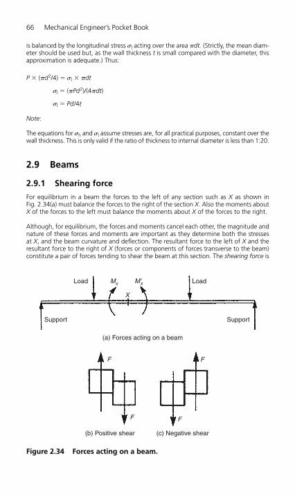
66 Mechanical Engineer’s Pocket Book
is balanced by the longitudinal stress �l acting over the area �dt. (Strictly, the mean diam-eter should be used but, as the wall thickness t is small compared with the diameter, thisapproximation is adequate.) Thus:
P � (�d2/4) � �l � �dt
�l � (�Pd2)/(4�dt)
�l � Pd/4t
Note:
The equations for �h and �l assume stresses are, for all practical purposes, constant over thewall thickness. This is only valid if the ratio of thickness to internal diameter is less than 1:20.
2.9 Beams
2.9.1 Shearing force
For equilibrium in a beam the forces to the left of any section such as X as shown in Fig. 2.34(a) must balance the forces to the right of the section X. Also the moments aboutX of the forces to the left must balance the moments about X of the forces to the right.
Although, for equilibrium, the forces and moments cancel each other, the magnitude andnature of these forces and moments are important as they determine both the stresses at X, and the beam curvature and deflection. The resultant force to the left of X and theresultant force to the right of X (forces or components of forces transverse to the beam)constitute a pair of forces tending to shear the beam at this section. The shearing force is
Load
(a) Forces acting on a beam
Load
Support Support
Mx
X
M�x
(b) Positive shear (c) Negative shear
F
F F
F
Figure 2.34 Forces acting on a beam.
H6508-Ch02.qxd 9/12/05 4:40 PM Page 66
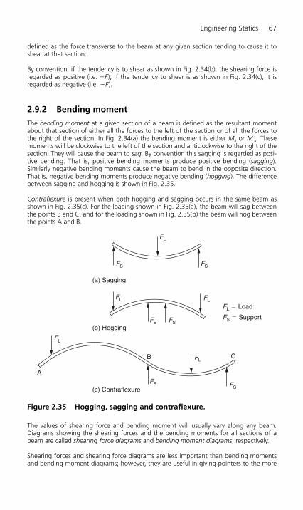
defined as the force transverse to the beam at any given section tending to cause it toshear at that section.
By convention, if the tendency is to shear as shown in Fig. 2.34(b), the shearing force isregarded as positive (i.e. �F); if the tendency to shear is as shown in Fig. 2.34(c), it isregarded as negative (i.e. �F).
2.9.2 Bending moment
The bending moment at a given section of a beam is defined as the resultant momentabout that section of either all the forces to the left of the section or of all the forces tothe right of the section. In Fig. 2.34(a) the bending moment is either Mx or M �x. Thesemoments will be clockwise to the left of the section and anticlockwise to the right of thesection. They will cause the beam to sag. By convention this sagging is regarded as posi-tive bending. That is, positive bending moments produce positive bending (sagging).Similarly negative bending moments cause the beam to bend in the opposite direction.That is, negative bending moments produce negative bending (hogging). The differencebetween sagging and hogging is shown in Fig. 2.35.
Contraflexure is present when both hogging and sagging occurs in the same beam asshown in Fig. 2.35(c). For the loading shown in Fig. 2.35(a), the beam will sag betweenthe points B and C, and for the loading shown in Fig. 2.35(b) the beam will hog betweenthe points A and B.
Engineering Statics 67
FL
FLFL
FL
FL
FL � Load
FS � Support
FSFS
FS
FS FS
FS
(a) Sagging
(b) Hogging
A
B C
(c) Contraflexure
Figure 2.35 Hogging, sagging and contraflexure.
The values of shearing force and bending moment will usually vary along any beam.Diagrams showing the shearing forces and the bending moments for all sections of abeam are called shearing force diagrams and bending moment diagrams, respectively.
Shearing forces and shearing force diagrams are less important than bending momentsand bending moment diagrams; however, they are useful in giving pointers to the more
H6508-Ch02.qxd 9/12/05 4:40 PM Page 67
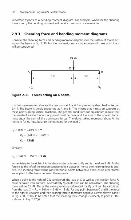
68 Mechanical Engineer’s Pocket Book
important aspects of a bending moment diagram. For example, wherever the shearingforce is zero, the bending moment will be at a maximum or a minimum.
2.9.3 Shearing force and bending moment diagrams
Consider the shearing force and bending moment diagrams for the system of forces act-ing on the beam in Fig. 2.36. For the moment, only a simple system of three point loadswill be considered.
24 kN
CB
3 m5 m
RB
A
RA
Figure 2.36 Forces acting on a beam.
It is first necessary to calculate the reactions at A and B as previously described in Section2.4.4. The beam is simply supported at A and B. This means that it rests on supports atthese points giving vertical reactions. The general conditions for equilibrium require thatthe resultant moment about any point must be zero, and the sum of the upward forcesmust equal the sum of the downward forces. Therefore, taking moments about A, themoment for RB must balance the moment for the load C:
RB � 8 m � 24 kN � 5 m
RB � (24 kN � 5 m)/8 m
RB � 15 kN
Similarly:
RA � 24 kN � 15 kN � 9 kN
Immediately to the right of A the shearing force is due to RA and is therefore 9 kN. As thisforce is to the left of the section considered it is upwards, hence the shearing force is posi-tive. The shearing force will be constant for all points between A and C as no other forcesare applied to the beam between these points.
When a point to the right of C is considered, the load at C as well as the reaction force RBmust be taken into account. Alternatively RB on its own can be considered. The shearingforce will be 15 kN. This is the value previously calculated for RB or it can be calculatedfrom the load C � RA � 24 kN � 9 kN � 15 kN. For any point between C and B the forceto the right is upwards and the shearing force is therefore negative as was shown earlierin Fig. 2.34. It should be noted that the shearing force changes suddenly at point C. Thisis shown in Fig. 2.37(a).
H6508-Ch02.qxd 9/12/05 4:40 PM Page 68
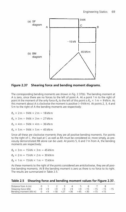
The corresponding bending moments are shown in Fig. 2.37(b). The bending moment atA is zero, since there are no forces to the left of point A. At a point 1 m to the right ofpoint A the moment of the only force RA to the left of this point is RA � 1 m � 9 kN m. Asthis moment about A is clockwise the moment is positive (�9 kN m). At points 2, 3, 4 and5 m to the right of A the bending moments are respectively:
RA � 2 m � 9 kN � 2 m � 18 kN m
RA � 3 m � 9 kN � 3 m � 27 kN m
RA � 4 m � 9 kN � 4 m � 36 kN m
RA � 5 m � 9 kN � 5 m � 45 kN m
Since all these are clockwise moments they are all positive bending moments. For pointsto the right of C, the load at C as well as RA must be considered or, more simply, as pre-viously demonstrated RB alone can be used. At points 5, 6 and 7 m from A, the bendingmoments are respectively:
RB � 3 m � 15 kN � 3 m � 45 kN m
RB � 2 m � 15 kN � 2 m � 30 kN m
RB � 1 m � 15 kN � 1 m � 15 kN m
As these moments to the right of the points considered are anticlockwise, they are all posi-tive bending moments. At B the bending moment is zero as there is no force to its right.The results are summarized in Table 2.5.
Engineering Statics 69
SFdiagram
BMdiagram
A B
9 kN
C
�15 kN
45 kN m
(a)
(b)
Figure 2.37 Shearing force and bending moment diagrams.
Table 2.5 Shearing force and bending moment values for Figure 2.37.
Distance from A (m) 0 1 2 3 4 5 6 7 8Shearing force (kN) �9 �9 �9 �9 �9 �9 �15 �15 �15 �15Bending moment (kN m) 0 �9 �18 �27 �36 �45 �30 �15 �15
H6508-Ch02.qxd 9/12/05 4:40 PM Page 69
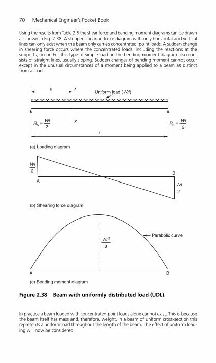
Using the results from Table 2.5 the shear force and bending moment diagrams can be drawnas shown in Fig. 2.38. A stepped shearing force diagram with only horizontal and verticallines can only exist when the beam only carries concentrated, point loads. A sudden changein shearing force occurs where the concentrated loads, including the reactions at the supports, occur. For this type of simple loading the bending moment diagram also con-sists of straight lines, usually sloping. Sudden changes of bending moment cannot occurexcept in the unusual circumstances of a moment being applied to a beam as distinctfrom a load.
70 Mechanical Engineer’s Pocket Book
a x
x
l
Uniform load (W/l)
RB �2
WlRA �
2Wl
(a) Loading diagram
2
Wl
2
Wl
A
B
(b) Shearing force diagram
(c) Bending moment diagram
Parabolic curve
8
Wl 2
A B
Figure 2.38 Beam with uniformly distributed load (UDL).
In practice a beam loaded with concentrated point loads alone cannot exist. This is becausethe beam itself has mass and, therefore, weight. In a beam of uniform cross-section thisrepresents a uniform load throughout the length of the beam. The effect of uniform load-ing will now be considered.
H6508-Ch02.qxd 9/12/05 4:40 PM Page 70

Figure 2.38(a) shows a uniformly loaded beam of length l and weight W. The only pointloads being the reactions at the supports RA and RB. Since the loading is symmetrical RAand RB will both equal W/2. The shear force diagram shows maximum values at the pointsof support and zero shear at the midpoint. This time, however, the line joining the shear-ing force is a sloping line passing through the midpoint.
Take a section XX at a distance a from the left-hand support RA:
The shearing force at XX � (Wl/2) � (W � a)
Since this is the equation of a straight line the shear force diagram is shown in Fig. 2.38(b).Unlike the previous example, this time the bending moment diagram is not made up ofstraight lines but is a continuous curve with a maximum value at the midpoint.
The bending moment Mx at XX � [(Wl/2) � a] � [W � a � (a/2)]
Therefore:
Mx � W/2(la � a2) (1)
This is the equation of a parabola so, its first derivative will be a maximum when:
dMx/da � 0
Differentiating equation (1):
dMx/da � W/2(l � 2a) � 0
When:
a � l/2
The maximum bending moment occurs at the centre of the span which is only to beexpected with symmetrical loading. Hence substituting a � l/2 in equation (1):
Mmax � W/2[(l2/2) � (l2/4)] � Wl2/8
The bending moment diagram is shown in Fig. 2.38(c). Apart from the beam shown inFig. 2.38(a) where the uniform load resulted from gravity acting on the mass of the beamitself, the only other occasion when a beam is uniformly loaded is when it is carrying auniform panel of masonry.
More often, there is a combination of point loads and uniform loading as shown in theloading diagram Fig. 2.39(a).
(a) Calculate reactions RA and RC by taking moments about A:
(45 � 2) � (12 � 9) � 4.5 � (24 � 12) � 9RCThus: RC � 96 kN and RA � 81 kN
(b) Shearing forces (let x be any distance from A):
For 0 � x � 2, shear force � (81 � 12x) kN (1)For 2 � x � 9, shear force � (81 � 12x � 45) � (36 � 12x) kNFor 9 � x � 12, shear force � (81 � 12 � 9 � 45 � 96) � �24 kN
These results are depicted by straight lines as shown in Fig. 2.39(b)
Engineering Statics 71
H6508-Ch02.qxd 9/12/05 4:40 PM Page 71
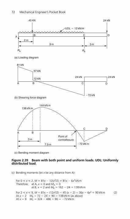
72 Mechanical Engineer’s Pocket Book
(c) Bending moments (let x be any distance from A):
For 0 � x � 2, M � 81x � 12(x2/2) � 81x � 6x2kN mTherefore: at A, x � 0 and MA � 0
at B, x � 2 and MB � 162 � 24 � 138 kN m
For 2 � x � 9, M � 81x � (12x2/2) � 45 (x � 2) � 36x � 6x2 � 90 kN m (2)At x � 2 MB � 72 � 24 � 90 � 138 kN m (as above)At x � 9 MC � 324 � 486 � 90 � �72 kN m
45 kN 24 kN
DCB
(a) Loading diagram
A2 m
RA
3 m9 m
24 kN
�72 kN
�72 kN m
24 kN
3 m
7.9 m
81 kN
57 kN
B
B
A
A
(b) Shearing force diagram
(c) Bending moment diagram
C
C
Point ofcontraflexure
D
D
12 kN
138 kN m144 kN m
RB
UDL � 12 kN/m
Figure 2.39 Beam with both point and uniform loads. UDL: Uniformlydistributed load.
H6508-Ch02.qxd 9/12/05 4:40 PM Page 72

The maximum bending moment occurs between the points B and C where dM/dx � 0.
Note this is the same point that the shearing force is also zero. From equation (2):
dM/dx � 36 � 12x � 0
Therefore:
x � 3 m
Substituting x � 3 in equation (2):
(36 � 3) � (6 � 32) � 90 � 144 kN m.
Thus the maximum bending moment is 144 kN m and it occurs at a point 3 m from A.
Contraflexure will occur when the bending moment is zero. That is, the positive root ofequation (2) when it is equated to zero.
36x � 6x2 � 90 � 0
Therefore:
x � 7.9 m (the only positive solution)
Therefore contraflexure occurs at a point 7.9 m from A.
2.9.4 Beams (cantilever)
As well as being simply supported as in the previous examples, beams may also be in theform of a cantilever. That is, only one end of the beam is supported and the remote endfrom the support is unsupported as shown in Fig. 2.40(a). The supported end of the beammay be built into masonry or it may be a projection from a simply supported beam. A typ-ical shearing force diagram and a typical bending moment diagram for a cantilever beamwith concentrated, point loads are shown in Fig. 2.40(b) and (c).
Engineering Statics 73
W1 W2 W3
l l 3l
(a) Loading diagram
Figure 2.40 Cantilever – point loads only.
H6508-Ch02.qxd 9/12/05 4:40 PM Page 73
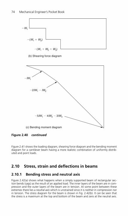
Figure 2.41 shows the loading diagram, shearing force diagram and the bending momentdiagram for a cantilever beam having a more realistic combination of uniformly distrib-uted and point loads.
2.10 Stress, strain and deflections in beams
2.10.1 Bending stress and neutral axis
Figure 2.42(a) shows what happens when a simply supported beam of rectangular sec-tion bends (sags) as the result of an applied load. The inner layers of the beam are in com-pression and the outer layers of the beam are in tension. At some point between theseextremes there lies a neutral axis which is unstrained since it is neither in compression norin tension. The stress diagram for the beam is shown in Fig. 2.42(b). It can be seen thatthe stress is a maximum at the top and bottom of the beam and zero at the neutral axis.
74 Mechanical Engineer’s Pocket Book
�W1
�(W1 � W2)
�(W1 � W2 � W3)
(b) Shearing force diagram
�lW1
�2lW1 � lW2
�5lW1 � 4lW2 � 3lW3
(c) Bending moment diagram
Figure 2.40 continued
H6508-Ch02.qxd 9/12/05 4:40 PM Page 74

Engineering Statics 75
3 m
(b) Shearing force diagram
(c) Bending moment diagram
UDL � 30 kN/m
40 kN
2 m
(a) Loading diagram
�90 kN
�190 kN
�135 kN m
�455 kN m
�130 kN
Figure 2.41 Cantilever – combined point and distributed loads.
Therefore a solid rectangular beam is less efficient than a typical I section beam which hasa much higher strength to weight ratio. In the I section beam the maximum stress is car-ried by the flanges at the top and bottom of the beam, and the lightweight web separ-ating the flanges carries little stress. In fact, to reduce the mass of the beam even furtherthe flange can often be perforated without appreciable loss of strength.
H6508-Ch02.qxd 9/12/05 4:40 PM Page 75
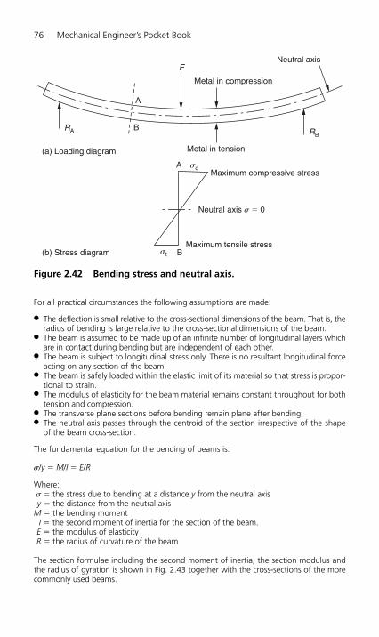
76 Mechanical Engineer’s Pocket Book
For all practical circumstances the following assumptions are made:
● The deflection is small relative to the cross-sectional dimensions of the beam. That is, theradius of bending is large relative to the cross-sectional dimensions of the beam.
● The beam is assumed to be made up of an infinite number of longitudinal layers whichare in contact during bending but are independent of each other.
● The beam is subject to longitudinal stress only. There is no resultant longitudinal forceacting on any section of the beam.
● The beam is safely loaded within the elastic limit of its material so that stress is propor-tional to strain.
● The modulus of elasticity for the beam material remains constant throughout for bothtension and compression.
● The transverse plane sections before bending remain plane after bending.● The neutral axis passes through the centroid of the section irrespective of the shape
of the beam cross-section.
The fundamental equation for the bending of beams is:
�/y � M/I � E/R
Where:� � the stress due to bending at a distance y from the neutral axisy � the distance from the neutral axis
M � the bending momentI � the second moment of inertia for the section of the beam.E � the modulus of elasticityR � the radius of curvature of the beam
The section formulae including the second moment of inertia, the section modulus andthe radius of gyration is shown in Fig. 2.43 together with the cross-sections of the morecommonly used beams.
Neutral axis s � 0
Maximum compressive stress
Metal in tension
B
A
Metal in compression
Neutral axis
B
A
F
RA RB
(a) Loading diagram
(b) Stress diagramMaximum tensile stress
st
sc
Figure 2.42 Bending stress and neutral axis.
H6508-Ch02.qxd 9/12/05 4:40 PM Page 76
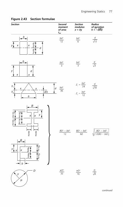
Figure 2.43 Section formulae
Section Second Section Radiusmoment modulus of gyrationof area z � I/y k � ��(I�/�����A�)Ixx
continued
D
8pD3
16
pD4
32
BD bdBD bd
3 3
12�
�( )
⎡
⎣⎢⎢⎢
⎤
⎦⎥⎥⎥
BD bdD
3 3
6�BD bd3 3
12�
Zbd
Zbd
1
2
24
12
�
�
2
2
bd3
36
d
3
bd2
3bd3
3
d
12bd2
6
bd3
12
Engineering Statics 77
y xd
x
b
d–2d–2
xx
b
d/3d
y1
y2
x x
b
B
yD–2
D–2
d–2d–2
P
yD
x
y
xd
b
x x y
B
D–2
D–2
d–2d–2
2b
2b �
d
18
H6508-Ch02.qxd 9/12/05 4:40 PM Page 77
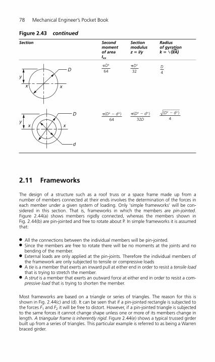
2.11 Frameworks
The design of a structure such as a roof truss or a space frame made up from a number of members connected at their ends involves the determination of the forces ineach member under a given system of loading. Only ‘simple frameworks’ will be con-sidered in this section. That is, frameworks in which the members are pin-jointed. Figure 2.44(a) shows members rigidly connected, whereas the members shown in Fig. 2.44(b) are pin-jointed and free to rotate about P. In simple frameworks it is assumedthat:
● All the connections between the individual members will be pin-jointed.● Since the members are free to rotate there will be no moments at the joints and no
bending of the member.● External loads are only applied at the pin-joints. Therefore the individual members of
the framework are only subjected to tensile or compressive loads● A tie is a member that exerts an inward pull at either end in order to resist a tensile load
that is trying to stretch the member.● A strut is a member that exerts an outward force at either end in order to resist a com-
pressive load that is trying to shorten the member.
Most frameworks are based on a triangle or series of triangles. The reason for this isshown in Fig. 2.44(c) and (d). It can be seen that if a pin-jointed rectangle is subjected tothe forces F1 and F2 it will be free to distort. However, if a pin-jointed triangle is subjectedto the same forces it cannot change shape unless one or more of its members change inlength. A triangular frame is inherently rigid. Figure 2.44(e) shows a typical trussed girderbuilt up from a series of triangles. This particular example is referred to as being a Warrenbraced girder.
78 Mechanical Engineer’s Pocket Book
Figure 2.43 continued
Section Second Section Radiusmoment modulus of gyrationof area z � I/y k � ��(I�/�����A�)Ixx
( )D d2 2
4
� �(D dD
4 4
32) �(D d4 4
64)
D4
D3
32
D4
64y
D
xx
D
xxy
d
H6508-Ch02.qxd 9/12/05 4:40 PM Page 78
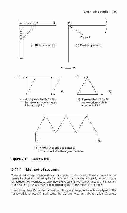
Engineering Statics 79
2.11.1 Method of sections
The main advantage of the method of sections is that the force in almost any member canusually be obtained by cutting the frame through that member and applying the principleof moments. For example, consider how the forces in three members cut by the imaginaryplane XX in Fig. 2.45(a) may be determined by use of the method of sections.
The cutting plane XX divides the truss into two parts. Suppose the right-hand part of theframework is removed. This will cause the left hand to collapse about the joint R1 unless
P
Pin-joint
(b) Flexible, pin-joint(a) Rigid, riveted joint
(c) A pin-jointed rectangular framework module has no inherent rigidity
(e) A Warren girder consisting of a series of linked triangular modules
(d) A pin-jointed triangular framework module is inherently rigid
F1F1
F2 F2
RA RB
Figure 2.44 Frameworks.
H6508-Ch02.qxd 9/12/05 4:40 PM Page 79
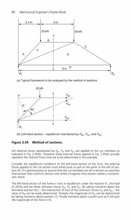
80 Mechanical Engineer’s Pocket Book
the external forces represented by FBF, FFE and FED are applied to the cut members as indicated in Fig. 2.45(b). Therefore these external forces applied in Fig. 2.45(b) actuallyrepresent the internal forces that are to be determined in this example.
Consider the equilibrium conditions of the left-hand section of the truss, the externalforces applied to the cut section must either push or pull on the joints to the left of sec-tion XX. It is good practice to assume that the cut members are all in tension as a positivefinal answer then confirms tension (tie) whilst a negative final answer implies a compres-sion (strut).
The left-hand section of the frame is now in equilibrium under the reaction R1, the loadof 20 kN and the three unknown forces FBF, FFE and FED. By taking moments about the left-hand reaction (R1) – the intersection of two of the unknown forces FFE and FED – thevalue of FBF can be easily determined. Similarly the magnitude of FED can be determinedby taking moments about position (1). Finally moments about a point such as P will givethe magnitude of the force in FE.
2.4 m 3 m
9 m
(a) Typical framework to be analysed by the method of sections
20 kN
B
C
E
FBF
FFE
FED
P
Q
(b) Left-hand section – equilibrium maintained by FBF, FFE, and FED
R1
90°
D
FA
R1 R2
x
x
x
x
30 kN
20 kN
Figure 2.45 Method of sections.
H6508-Ch02.qxd 9/12/05 4:40 PM Page 80
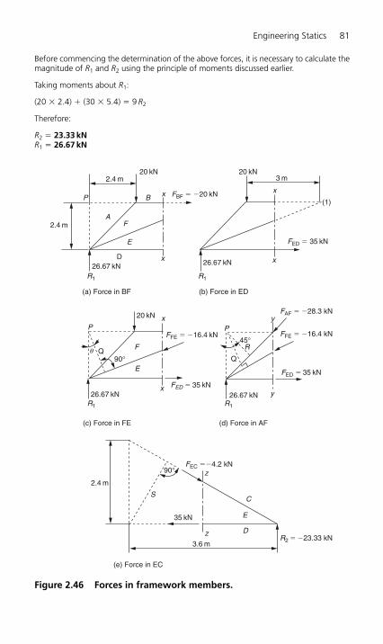
Before commencing the determination of the above forces, it is necessary to calculate themagnitude of R1 and R2 using the principle of moments discussed earlier.
Taking moments about R1:
(20 � 2.4) � (30 � 5.4) � 9 R2
Therefore:
R2 � 23.33 kNR1 � 26.67 kN
Engineering Statics 81
2.4 m20 kN
20 kN
20 kN3 m
(1)
FED � 35 kN
FAF � �28.3 kN
FFE � �16.4 kN
R2 � �23.33 kN
FEC ��4.2 kN
B FBF � �20 kNP
AF
F R
FFE � �16.4 kN
FED � 35 kN
FED � 35 kNE
z
S
z
C
E
D
3.6 m
E
D
P P
R1
R1
R1
R1
2.4 m
26.67 kN
26.67 kN
x
x y
yx
x
x
x26.67 kN
26.67 kN
35 kN
2.4 m
(a) Force in BF
(c) Force in FE
(e) Force in EC
(d) Force in AF
(b) Force in ED
90°
90°
45°Q
Qu
Figure 2.46 Forces in framework members.
H6508-Ch02.qxd 9/12/05 4:40 PM Page 81
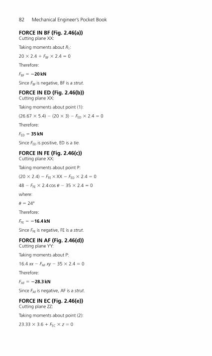
FORCE IN BF (Fig. 2.46(a))Cutting plane XX:
Taking moments about R1:
20 � 2.4 � FBF � 2.4 � 0
Therefore:
FBF � 20 kN
Since FBF is negative, BF is a strut.
FORCE IN ED (Fig. 2.46(b))Cutting plane XX:
Taking moments about point (1):
(26.67 � 5.4) � (20 � 3) � FED � 2.4 � 0
Therefore:
FED � 35 kN
Since FED is positive, ED is a tie.
FORCE IN FE (Fig. 2.46(c))Cutting plane XX:
Taking moments about point P:
(20 � 2.4) � FFE � XX � FED � 2.4 � 0
48 � FFE � 2.4 cos � 35 � 2.4 � 0
where:
� � 24°
Therefore:
FFE � �16.4 kN
Since FFE is negative, FE is a strut.
FORCE IN AF (Fig. 2.46(d))Cutting plane YY:
Taking moments about P:
16.4 xx � FAF xy � 35 � 2.4 � 0
Therefore:
FAF � 28.3 kN
Since FAF is negative, AF is a strut.
FORCE IN EC (Fig. 2.46(e))Cutting plane ZZ:
Taking moments about point (2):
23.33 � 3.6 � FEC � z � 0
82 Mechanical Engineer’s Pocket Book
H6508-Ch02.qxd 9/12/05 4:40 PM Page 82
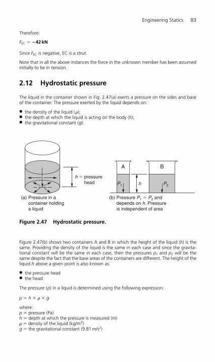
Engineering Statics 83
Therefore:
FEC � �42 kN
Since FEC is negative, EC is a strut.
Note that in all the above instances the force in the unknown member has been assumedinitially to be in tension.
2.12 Hydrostatic pressure
The liquid in the container shown in Fig. 2.47(a) exerts a pressure on the sides and baseof the container. The pressure exerted by the liquid depends on:
● the density of the liquid (�);● the depth at which the liquid is acting on the body (h);● the gravitational constant (g).
h � pressure head
(a) Pressure in a container holding a liquid
(b) Pressure P1 � P2 and depends on h. Pressure is independent of area
P1 P2h
A B
Figure 2.47 Hydrostatic pressure.
Figure 2.47(b) shows two containers A and B in which the height of the liquid (h) is thesame. Providing the density of the liquid is the same in each case and since the gravita-tional constant will be the same in each case, then the pressures p1 and p2 will be thesame despite the fact that the base areas of the containers are different. The height of theliquid h above a given point is also known as:
● the pressure head● the head.
The pressure (p) in a liquid is determined using the following expression:
p � h � � � g
where:p � pressure (Pa)h � depth at which the pressure is measured (m)� � density of the liquid (kg/m3)g � the gravitational constant (9.81 m/s2)
H6508-Ch02.qxd 9/12/05 4:40 PM Page 83

84 Mechanical Engineer’s Pocket Book
ExampleFigure 2.48 shows a container filled with paraffin to a depth of 2 m. Determine the pres-sures p1 and p2, given the density of paraffin � 800 kg/m3 and g � 9.81 m/s2.
p1 � h1 � � � g � 2 m � 800 kg/m3 � 9.81 m/s2 � 15696 Pa or 15.696 kPa
p2 � h2 � � � g � 1 m � 800 kg/m3 � 9.81 m/s2 � 7848 Pa or 7.848 kPa
At the half depth point the pressure is half that at the bottom of the container. At the sur-face the pressure is zero since there is no depth. Therefore the pressure is proportional tothe depth at which it is measured.
P1
P22 m
1 m
Figure 2.48 Factors affecting pressure.
2.12.1 Thrust on a submerged surface
Consider the rectangular container shown in Fig. 2.49. It was shown in the previousexample that the half pressure occurs at the half depth. Since the pressure varies fromzero at the surface to a maximum at the full depth the pressure at the half depth is theaverage pressure (pA). That is:
pA � (p1 � p2)/2 � p2/2 (since p1 � 0)
Therefore the force (thrust) acting on the side of the container will be the submerged areaof the side (AS) multiplied by the average pressure (pA). That is:
FS � pA � AS
where:FS � force (thrust) acting on the side of the container (N)pA � average pressure (Pa)AS � submerged area of the side of the container (m2)
Note:
1. The force is assumed to act at the centre of area of the side of the container.2. The force acting on the bottom of the container is calculated using the maximum pres-
sure and not the average pressure.
ExampleFigure 2.49 shows a rectangular tank with a base area of 9 m2. It is filled with a water toa depth of 2 m. Taking g � 9.81 m/s2, calculate:
(i) The pressure acting on the base of the tank.(ii) The force acting on the base of the tank.(iii) The average pressure acting on the sides of the tank.
H6508-Ch02.qxd 9/12/05 4:40 PM Page 84
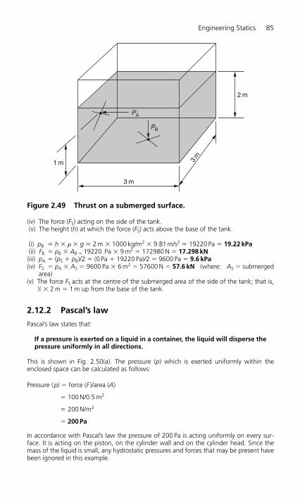
Engineering Statics 85
(iv) The force (FS) acting on the side of the tank.(v) The height (h) at which the force (FS) acts above the base of the tank.
(i) pB � h � � � g � 2 m � 1000 kg/m2 � 9.81 m/s2 � 19220 Pa � 19.22 kPa(ii) FB � pB � AB � 19220 Pa � 9 m2 � 172980 N � 17.298 kN(iii) pA � (pS � pB)/2 � (0 Pa � 19220 Pa)/2 � 9600 Pa � 9.6 kPa(iv) FS � pA � AS � 9600 Pa � 6 m2 � 57600 N � 57.6 kN (where: AS � submerged
area)(v) The force FS acts at the centre of the submerged area of the side of the tank; that is,
1⁄2 � 2 m � 1 m up from the base of the tank.
2.12.2 Pascal’s law
Pascal’s law states that:
If a pressure is exerted on a liquid in a container, the liquid will disperse thepressure uniformly in all directions.
This is shown in Fig. 2.50(a). The pressure (p) which is exerted uniformly within theenclosed space can be calculated as follows:
Pressure (p) � force (F )/area (A)
� 100 N/0.5 m2
� 200 N/m2
� 200 Pa
In accordance with Pascal’s law the pressure of 200 Pa is acting uniformly on every sur-face. It is acting on the piston, on the cylinder wall and on the cylinder head. Since themass of the liquid is small, any hydrostatic pressures and forces that may be present havebeen ignored in this example.
1 m
PA
PB
3 m
2 m
3m
Figure 2.49 Thrust on a submerged surface.
H6508-Ch02.qxd 9/12/05 4:40 PM Page 85
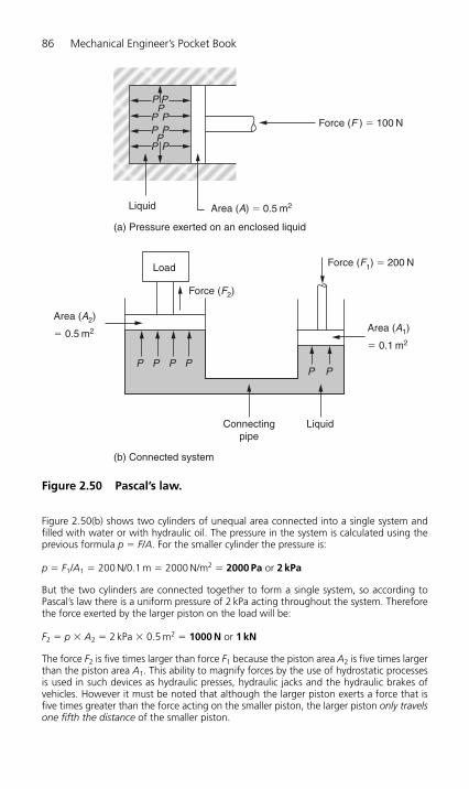
86 Mechanical Engineer’s Pocket Book
Figure 2.50(b) shows two cylinders of unequal area connected into a single system andfilled with water or with hydraulic oil. The pressure in the system is calculated using theprevious formula p � F/A. For the smaller cylinder the pressure is:
p � F1/A1 � 200 N/0.1 m � 2000 N/m2 � 2000 Pa or 2 kPa
But the two cylinders are connected together to form a single system, so according toPascal’s law there is a uniform pressure of 2 kPa acting throughout the system. Thereforethe force exerted by the larger piston on the load will be:
F2 � p � A2 � 2 kPa � 0.5 m2 � 1000 N or 1 kN
The force F2 is five times larger than force F1 because the piston area A2 is five times largerthan the piston area A1. This ability to magnify forces by the use of hydrostatic processesis used in such devices as hydraulic presses, hydraulic jacks and the hydraulic brakes ofvehicles. However it must be noted that although the larger piston exerts a force that isfive times greater than the force acting on the smaller piston, the larger piston only travelsone fifth the distance of the smaller piston.
Liquid Area (A) � 0.5 m2
Force (F2)
Connectingpipe
Liquid
Area (A2)
� 0.5 m2 Area (A1)
� 0.1 m2
Load
Force (F ) � 100 N
(a) Pressure exerted on an enclosed liquid
(b) Connected system
Force (F1) � 200 N
P PP
P PP P
PP
P P P PP P
P
Figure 2.50 Pascal’s law.
H6508-Ch02.qxd 9/12/05 4:40 PM Page 86

3Engineering Dynamics
3.1 Engineering dynamics
As stated at the beginning of Chapter 2, engineering mechanics can be divided into sta-tics and dynamics. Chapter 3 is concerned with dynamics which is the study of objects inmotion.
3.2 Work
When a force is applied to a body so that it causes the body to move, the force is said tobe doing work. The work done is the product of the distance moved in metres (m) andthe applied force in newtons (N) measured in the direction of motion. Therefore the workdone is measured in newton metres and the unit of work is joule (J) where 1 Nm � 1 J.
Figure 3.1(a) shows a body is being moved by a force F along a horizontal plane. Since theforce is acting on the body parallel to the horizontal plane, the work done is product of
F � 50 N
s � 3 m
F � 50 N
FH � 50 cos 30°
s � 3 m
(a)
(b)
a
Figure 3.1 Work. (a) Work done by a force F. (b) Work done by theforce FH.
H6508-Ch03.qxd 9/12/05 4:38 PM Page 87

the force F (N) and the distance s (m). If the force is 50 N and the distance is 3 m, then thework done is:
50 N � 3 m � 150 Nm � 150 J
In Fig. 3.1(b) the force is inclined through the angle � to the direction of motion. In thiscase the force vector has to be resolved into its vertical and horizontal components as shown. The component force that is parallel to the direction of motion of the body is F cos �. Therefore the work done is s � F cos � joules. If the force (F ) is again 50 N, thedistance (s) is again 3 m and the angle � is 30° the work done will be:
W � 3 m � 50 N � 0.866 � 129.9 Nm � 129.9 J
3.3 Energy
Anything capable of doing work is said to posses energy. Energy exists in various formsand may be considered as ‘stored work’ awaiting to be used. For example:
● Chemical energy is absorbed or released when a reaction occurs (e.g. the combustionof fossil fuels).
● Atomic energy is liberated by splitting or combining atomic particles. Splitting atomicparticles is called fission and combining atomic particles is called fusion. These reac-tions produce large amounts of heat energy.
● Heat energy can be subdivided into sensible heat energy and latent heat energy.Sensible heat energy is the energy taken in or given out when a solid, liquid or gas risesin temperature or falls in temperature. Latent heat energy is the energy required tochange the state of a solid, liquid or gas at a constant temperature.
● Mechanical energy can be subdivided into potential energy, kinetic energy and strainenergy:1. Potential energy (also known as conserved energy) is the energy possessed by a
body due to position. For example when work has been done to raise the hammerof a pile driver the work is stored in the hammer as potential energy.
2. Kinetic energy is the energy possessed by a body by virtue of its velocity. For example ifthe hammer of the pile driver is allowed to fall, the potential energy is reduced indirect proportion to the loss of height. The kinetic energy increases in direct pro-portion to the gain in velocity. The potential energy is being converted into kineticenergy due to the motion of the hammer. At the instant of the impact of the ham-mer on the pile all the potential energy is converted into kinetic energy which isused to do work, namely to drive the pile into the ground. Kinetic energy � 1⁄2mv2.
3. Strain energy (also known as conserved energy) is the energy stored in a piece ofstrained elastic material. For example when a metal bar is stretched by a tensileforce, work is done on the bar. Provided that the strain is kept within the elasticrange for the material, the work done in stretching the bar is stored up as strainenergy. This energy can be regained on removal of the straining force. The sameargument applies when a bar is twisted as in a torsion spring.
3.3.1 Conservation of energy
The law of conservation of energy states that: Energy can be neither created nor destroyedbut is convertible from one form to another.
For example, in a power station, the chemical energy of the fuel is released by combustionand is converted into thermal energy which, in turn, produces steam in a boiler. The steam
88 Mechanical Engineer’s Pocket Book
H6508-Ch03.qxd 9/12/05 4:38 PM Page 88

drives a turbine which converts the energy in the steam into mechanical energy. Thismechanical energy is converted into electrical energy by the alternator driven by the turbine.During these conversion processes there will be loss of energy due to the inefficiency of theequipment used. This ‘lost’ energy cannot be destroyed (law of conservation of energy) butis converted into other forms of energy that do not contribute to useful work. For examplework done in overcoming friction by heating the bearing surfaces and the lubricating oil.
3.4 Power
Power is the rate of doing work and can be expressed mathematically as:
Power (W) � work done (J)/time taken (s) � force (N) � velocity (m/s)
The unit of power is the watt (W) where 1 watt equals work done at the rate of 1 J/s.
ExampleA body of weight 5 kN is to be raised through a height of 15 m in 10 s. Calculate thepower required.
Work done � force (weight) � distance moved � 5 kN � 15 m � 75 kNm � 75 kJ
Power required � work done/time � 75 kJ/10 s � 7.5 kW (assuming 100% efficiency).
3.5 Efficiency
Efficiency is the measure of the ‘usefulness’ of a machine, process or operation.
Efficiency (�) � [work (or power) output]/[work (or power) input]
Efficiency can be expressed as a percentage (%) or as a decimal fraction of 1 (per-unit effi-ciency). In practice the efficiency of a device can never achieve 100% or 1.
ExampleIf the efficiency of the hoist in the previous example is 80%, calculate the actual powerrequired.
Efficiency (%) � (power output � 100)/power input
Therefore
80% � 7.5 kW/power input
Hence
Power input � (7.5 � 100)/80
� 9.375 kW
3.6 Velocity and acceleration
● Speed is a scalar quantity since it has magnitude only (e.g. 30 km/h).● Velocity is a vector quantity since it has magnitude and direction (e.g. 30 km/h due north).● Acceleration is the rate of change of velocity.
Engineering Dynamics 89
H6508-Ch03.qxd 9/12/05 4:38 PM Page 89
3.6.1 Speed
Speed is the rate of change of distance. That is: speed � distance/time. Typical units ofspeed are kilometres per hour (km/h) and metres per second (m/s).
Note: s (roman type) stands for seconds; s (italic type) stands for distance. They may bothappear in the same calculation.
3.6.2 Velocity
Velocity is the rate of change of distance in a particular direction. A body moving in astraight line is said to have uniform velocity in a straight line. Uniform velocity occurswhen a body moving in a straight line covers equal distances in equal interval of time.
Velocity � ds/dt in a particular direction
3.6.3 Acceleration
Acceleration is the rate of change of velocity. That is:
● Uniform acceleration occurs when a body experiences equal changes in velocity in equaltime intervals. The basic unit of acceleration � m/s2.
● Retardation or deceleration is the reverse process to acceleration. It is frequently referredto as negative acceleration.
3.6.4 Equations relating to velocity and acceleration
The symbols that will be used in the following equations are:v1 � initial velocity in metres per second (m/s);v2 � the final velocity in metres per second (m/s);a � acceleration in metres per second squared (m/s2);s � the distance travelled in metres (m);t � the time taken in seconds (s).
1. Average velocity � (v1 � v2)/22. Final velocity v2 � v1 � at3. Distance travelled s � (v1 � v2)t/24. Distance travelled s � v1t � 1⁄2at2
5. Acceleration a � (v2 � v1)/t6. Acceleration a � (v2
2 � v12)/2s
3.6.5 Momentum
The linear momentum of a body is defined by:
Momentum � mass � velocity � mv
The basic unit of momentum is kg m/s.
3.6.6 Newton’s laws of motion
1. Newton’s first law states that: a body continues in its state of rest, or uniform motion ina straight line, unless acted upon by a resultant force. That is, a body will not move,change its direction of motion, or accelerate unless it is compelled to by some external
90 Mechanical Engineer’s Pocket Book
H6508-Ch03.qxd 9/12/05 4:38 PM Page 90

force. Therefore a force can be defined as that which changes or tends to change themotion of a body upon which it acts.
2. Newton’s second law states that: the rate of change of momentum of a body is pro-portional to the resultant force applied to that body and takes place in the direction inwhich the force is applied
3. Newton’s third law states that: for every acting force there is an equal and oppositereaction force (see Section 3.6.8).
From Newton’s second law of motion it is apparent that:
The applied force � rate of change of momentum
The applied force � change in momentum/time
Thus if a force F causes a mass m to experience a change in velocity from v1 to v2 in time t, then:
F � (mv2 � mv1)/t
F � m(v2 � v1)/t
F � ma where a � (v2 � v1)/t
Therefore
F � ma � constant
By choosing unit force (N), unit mass (kg) and unit acceleration (m/s2), the constantbecomes 1 and:
F � ma
ExampleA motor car of mass 4000 kg accelerates from 10 to 60 km/h in 10 s. Determine theapplied force required to produce the acceleration.
v2 � v1 � at (equation (2) Section 3.6.4)
Where:v2 � 60 km/h � 16.67 m/sv1 � 10 km/h � 2.78 m/st � 10 s
Then:a � (v2 � v1)/ta � (16.67 � 2.78)/10a � 1.39 m/s2
Since:F � maF � 4000 kg � 1.39 m/s2
F � 5.56 kN
3.6.7 Gravity
Weight is a force. It is the effect of the force of gravity acting on the mass of a body pro-ducing, or trying to produce, an acceleration. Note the acceleration of 9.81 m/s2 is anaverage value on planet earth. It varies slightly from place to place but 9.81 m/s2 is accept-able for all practical purposes. The acceleration due to gravity is given the symbol g, there-fore the expression:
F � ma becomes F � mg in calculations involving gravity.
Engineering Dynamics 91
H6508-Ch03.qxd 9/12/05 4:38 PM Page 91
[On planet earth, the force F exerted by a mass of 5 kg � 5 � 9.81 � 49.05 kN. Since thegravitational attraction of the moon is approximately 1/6 that of the gravitational effectof planet earth, the force F exerted by a mass of 5 kg � 5 � (9.81/6) � 8.175 kN on themoon.]
3.6.8 Conservation of momentum
The Principle of the Conservation of Linear Momentum is derived from Newton’s third lawof motion. That is, for every acting force there is an equal and opposite reaction force.The Principle of Conservation of Linear Momentum states that: the total momentum ofas system, in a given direction, remains constant unless an external force is applied to thesystem in that given direction. This principle enables impact problems involving only inter-nal forces to be easily resolved.
Consider the firing of a projectile from a gun. Equal and opposite forces are acting on theprojectile and the gun will cause the projectile to move forward and the gun to movebackwards. Since there are no external forces involved, if both gun and projectile hadequal masses they would move with equal velocity. Fortunately, in practice, the gun has amuch greater mass than the projectile so that the recoil is much less than the forwardmovement of the projectile.
ExampleA body P of mass 15 kg moving with a velocity of 30 m/s when it collides with a secondbody Q of mass 5 kg which is moving in the same direction at 5 m/s. Determine the com-mon velocity of the two bodies after impact.
By the Principle of the Conservation of Linear Momentum:
Momentum before impact � momentum after impact
Mass � velocity before impact � mass � velocity after impact
15 kg � 30 m/s � 5 kg � 5 m/s � (15 kg � 5 kg)vI where vI � velocity after impact
vI � 23.75 m/s
Figure 3.10(a) shows that had the two bodies been moving in opposite directions beforeimpact then the velocity of the second body Q would be considered as a negative quantityand the calculation would be as follows:
Momentum before impact � momentum after impact
15 kg(�30 m/s) � 5 kg(�5 m/s) � (15 kg � 5 kg)vI
vI � 21.25 m/s
3.6.9 Impact of a fluid jet on a fixed body● If the jet is deflected from its line of motion then, from Newton’s first law, a force must
be acting on it.● If the force that is acting on the jet is proportional to the rate of change of momentum
and acts in the direction of the change of momentum, then Newton’s second law isapplicable.
● If the force exerted by the body on the jet to change its momentum then this forcemust be equal and opposite to the force exerted by the jet on the body.
92 Mechanical Engineer’s Pocket Book
H6508-Ch03.qxd 9/12/05 4:38 PM Page 92

Since this example involves the impact of a fluid jet, then it is concerned with jet flow rateand Newton’s second law of motion can be written as:
Force � rate of change of momentum� (mass � change of velocity)/time taken� mass flow rate � change of velocity in the direction of the force
ExampleA water jet of 50 mm diameter impacts perpendicularly on a fixed body with a velocity of75 m/s. Determine the force acting up the body.
Assume that the jet of water will spray out radially when it impacts on the body; that is,it is deflected through an angle of 90°. Therefore the jet will lose all its momentum atright angles to the body as shown in Fig. 3.2.
Area of jet � (�/4) � (50/1000)2m2 � 6.25� �10�4
Volume flow rate � 6.25� � 10�4m2 � 75 m/s � 0.047� m3/s
Mass flow rate (water) � volume flow rate � density of water
� 0.047� m3/s � 103kg/m3 � 47� kg/s
Force acting on the body � mass flow rate � change in velocity
Note : the change in velocity is from 75 m/s to 0 m/s immediately the jet impacts the body.
Therefore:
Force acting on the body � 47� kg/s � 75 m/s � 3525 N � 3.525 kN
3.6.10 Inertia
Newton’s first law of motion states that a body remains in a state of rest or uniform motionin a straight line unless acted on by an external force. This resistance to change is referredto as the inertia of a body and the amount of inertia depends on the mass of the body.Therefore it takes a great deal more force to accelerate a fully laden heavy goods vehiclefrom rest than the force required to produce the same acceleration in a bicycle from rest.
3.6.11 Resisted motion
The following points should be carefully noted when using the expression F � ma:
● F can refer to both an accelerating force or a retarding force.● It is often necessary to determine the value of an acceleration or a retardation, using the
equations of motion considered earlier, when working out engineering calculations.
Engineering Dynamics 93
∅50 mm
75 m/s
Jet of waterRigid plate
Figure 3.2 Impact of a fluid on a fixed body.
H6508-Ch03.qxd 9/12/05 4:38 PM Page 93

● When a force causing the acceleration of a body is resisted by a force trying to retard(decelerate) the body, the body is said to be subject to resisted motion.
Figure 3.3(a) shows a force P acting on a mass m against a resistance R and producing anacceleration a. The accelerating force Fa � (P � R) and Fa � ma is written P � R � ma.
Figure 3.3(b) shows a suspended body of mass m. Let P be the tension in the rope sus-pending the body:
1. For motion up or down at constant speed, or when the body is at rest, the accelera-tion equals zero therefore the accelerating force (F ) also equals zero.
2. For motion downwards with acceleration a, W is greater than P where W � mg. Thenthe accelerating force F � (W � P) so that (W � P) � ma.
3. For motion upwards with acceleration a, F � (P � W ) so that (P � W ) � ma.
Figure 3.3(c) shows a body on a smooth inclined plane. For this example any friction willbe ignored. The component force of weight W acting down the plane � W sin �, whereW � mg (N):
1. If P is greater than W sin �, the body moves up the plane with acceleration a. Theaccelerating force F � P � W sin � so that P � W sin � � ma.
2. If W sin � is greater than P, the body moves down the plane with acceleration a. Thenthe accelerating force F � W sin � � P so that W sin � � P � ma.
ExampleA body of mass of 600 kg has a resistance to motion of 400 N. Determine the total forceto be applied to the body to produce a uniform acceleration of 3 m/s.
Let the total force required � P.
Then: The accelerating force F � (P � 400)
Since F � ma Then: (P � 400 N) � 600 kg � 3 m/s
Therefore: P � 400 N � 1800 N � 2200 N
ExampleA passenger lift of mass 1500 kg starts from rest and reaches an upward velocity of 5 m/sin a distance of 10 m. Determine the tension in the lift cable if the acceleration is constant.Take g � 9.81 m/s2.
To find the acceleration use the expression (v2)2 � (v1)2 � 2as
Therefore:
52m/s � 0 � 2 m/s � a �10 m
So:
a � 25/(2 �10) � 1.25 m/s2
Whilst the lift is stationary, the tension in the cable is only due to the force of gravity act-ing on the lift (mg) which is equal to 1500 kg � 9.81 m/s2 � 14715 N. Since the lift isaccelerating upwards the tension P is greater than 14715 N.
Let P � the tension in the lift cable.
Then, the accelerating force F � P � 14715 � ma � 1500 � 1.25 m/s2.
Therefore: P � 14715 � 1500 � 1.25 � 16590 N � 16.59 kN.
94 Mechanical Engineer’s Pocket Book
H6508-Ch03.qxd 9/12/05 4:38 PM Page 94

Engineering Dynamics 95
Resistance (R) N Force (P ) N
Acceleration (a) m/s2
Acceleration (a) m/s2
(a)
(b)
Mass (m) kg
Mass (m) kg
Tension (P ) N
Weight W � mg (N)
(c)
Force (P ) N
Mass (m) kg
Acceleration (a) m/s
2
(W sin u) N
u Weight (W � mg) N
Figure 3.3 Resisted motion. (a) Resisted motion in a horizontalplane, (b) Resisted motion of a suspended body, (c) Resisted motionon an inclined plane.
H6508-Ch03.qxd 9/12/05 4:38 PM Page 95
3.7 Angular motion
When a rigid body rotates about a fixed axis all points on the body are constrained tomove in a circular path. Therefore in any given period of time all points on the body willcomplete the same number of revolutions about the axis of rotation; that is, the speed ofrotation is referred to in terms of revolutions per minute (rev/min). However, for manyengineering problems it is often necessary to express the speed of rotation in terms of theangle in radians turned through in unit time.
3.7.1 The radian
A radian is the angle subtended at the centre of a circle by an arc equal in length to theradius of that circle. This is shown in Fig. 3.4(a). The relationship between arc length,radius and angle in radians is shown in Fig. 3.4(b).
96 Mechanical Engineer’s Pocket Book
1 radian
r
r
r
(a)
s
r
r
u
(b)
Figure 3.4 (a) The radian (r � radius of the circle), (b) Relationshipbetween arc length (s), radius (r) and angle (��) in radians.
H6508-Ch03.qxd 9/12/05 4:38 PM Page 96
Where:
s � length of arc� � angle in radiansr � radius of the circle
From the definition of a radian:
s/r � � therefore s � r�
In the expression s � r� if s is equal to the circumference of a circle then:
2�r � r� therefore 2� � �
That is, 1 revolution � 2� radians (�360°)Similarly 1 radian � 360/2� � 57.3° (approximately).
3.7.2 Angular displacement
In linear motion the symbol s represents the distance travelled in a straight line; that is, thelinear displacement. In angular motion, the Greek letter � is the corresponding symbol forthe displacement measured in radians.
3.7.3 Angular velocity
A rigid body rotating about a fixed axis O at a uniform speed of n rev/s turns through 2�radians (rad) in each revolution. Therefore the angular velocity � (Greek letter omega) isgiven by the expression:
� � 2�n rad/s
Further, if the body rotates through an angle of � radians in time t seconds then, if thatmotion is uniform,
The angular velocity � � �/t rad/s
Note that angular velocity has no linear dimensions.
3.7.4 The relationship between angular and linear velocity
Consider the point A on the outer rim of the solid body shown in Fig. 3.5.
If the body rotates through � (rad) in t (seconds), and using length of arc � angle in radians � radius
s � r�
then to obtain the average velocity divide both sides of the expression by t so that:
s/t � r(�/t)
but
s/t � v and �/t � �
Engineering Dynamics 97
H6508-Ch03.qxd 9/12/05 4:38 PM Page 97

Therefore:
v � r� or linear velocity � angular velocity � radius.
Note:
1. The point B on the body has the same angular velocity as A but has a smaller linearvelocity since it has a smaller radius.
2. If the radius r is in metres and the angular velocity � is expressed in rad/s, then the linear velocity v is expressed in m/s. Sometimes the angular velocity is expressed inrev/min. It is necessary to convert rev/min to rad/s before substituting in expressionssuch as v � r�:
N (rev/min) � 2�N (rad/min) � 2�N/60 (rad/s)
3.7.5 Angular acceleration
A similar relationship to that of linear and angular velocity exist between linear and angu-lar acceleration. That is:
a � r�
where:a � linear acceleration, r � radius, � (Greek letter alpha) � angular acceleration.
Section 3.6.4 listed the expressions for the relationships between linear velocity and accel-eration. Similarly there is a set of expression for the relationships between angular velocityand acceleration. These are:
�2 � �1 � �t �1 � initial angular velocity� � [(�1 � �2)/2] � t �2 � final angular velocity� � �1t � 1⁄2 �t2 � � angular acceleration�2
2 � �12 � 2�� � � angle of rotation
� � �2t � 1⁄2 �t2 t � time taken
3.7.6 Torque
Torque is the turning moment of a force. When a force produces the rotation of a bodywithout translation motion, there must be a second force acting upon the body equal and
98 Mechanical Engineer’s Pocket Book
A
r
B
su
v
Figure 3.5 Relationship between angular and linear velocity.
H6508-Ch03.qxd 9/12/05 4:38 PM Page 98
opposite to the first so that the resultant force is zero. That is, the forces are in equilib-rium. Consider the spanner and nut shown in Fig. 3.6(a). When a force F1 is applied to theend of the spanner, an equal and opposite parallel force F2 occurs at the nut. If this werenot so, there would be motion of translation in the direction of force F1. When two equaland opposite forces act on a body they are said to form a couple.
Engineering Dynamics 99
d
F2
F1
(a)
sO
r
A
F
u
(b)
Figure 3.6 (a) Torque (turning moment). (b) Work done by a torque.
H6508-Ch03.qxd 9/12/05 4:38 PM Page 99

Torque (T ) � magnitude of the applied force (F1) � length of the torque arm (d)
Where:
T � torque (Nm)F � force (N) and d � moment arm (m)
3.7.7 Work done by a torque
Consider the work done by a force F (N) acting at right angles to the moment arm OA oflength r (m) and rotating through an angle � rad as shown in Fig. 3.6(b).
Work done � linear distance moved by a force � s � F (Nm or J)
But:
s � r� (m)
Therefore:
work done � r� � F � Fr � �
But:
torque T � Fr
Therefore:
work done � T� (Nm or J)
Work done by a torque � torque � angle of rotation in radians
ExampleA flywheel rotates at 2400 rev/min. It is suddenly subjected to a breaking torque whichresults in an angular retardation (deceleration) of 10 m/s2. Calculate:
(a) the time taken to slow the flywheel down to 600 rev/min;(b) the angular velocity of the flywheel after it has rotated through 300 revolutions from
the start of its deceleration.
(a) Apply the equation:
�2 � �1 � �t (Section 3.7.5)
Where:
�1 � initial angular velocity � (2400 rev/min � 2�) /60 rad/s�2 � angular velocity after time t � (600 � 2�)/60 rad/s� � angular acceleration � �10 m/s2 (the minus sign indicates a deceleration)
Therefore:
(600 � 2�)/60 � (2400 rev/min � 2�)/60 � (�10)t10t � (1800 � 2�)/60
Therefore:
t � 18.8 s
100 Mechanical Engineer’s Pocket Book
H6508-Ch03.qxd 9/12/05 4:38 PM Page 100
(b) Apply equation:
(�2)2 � (�1)2 � 2�� (Section 3.7.5)
Where:
�2 � angular velocity after rotating through 300 rev�1 � (2400 rev/min � 2�)/60 rad/s � 251.33 rad/s� � �10 rad/s2
� � 300 � 2� rad
Then:
�22 � 251.332 � 2 � (�10) � 600�
� 63166.8 � 37699.1
� 159.6 rad/s or
� (159.6 � 60)/2�
� 1524 rev/min
3.7.8 Centripetal acceleration and centripetal force
The dictionary definition of centripetal acceleration states that it is the accelerationdirected towards the centre of curvature of the path of a body which is moving along thatpath with constant speed. Its value is v2/r where v is the speed and r is the radius of curva-ture or its value can be expressed as �2r where � is the angular velocity.
Figure 3.7(a) shows a body of mass m moving along a circular path of radius r and centre Owith a constant angular velocity �. When the body is a point P it possesses an instanta-neous linear velocity v tangential to the circumference of the circle along which it is trav-elling. During an incremental period of time, �t, the body moves along the circumferenceof the circle from P to Q. The angle subtended by this translation from P to Q is ��.Although the body is moving at constant speed, it is not moving along the same line ofaction. Therefore, there is a change in the velocity of the body. Since there is a change ofvelocity with respect to time the body is, by definition, subjected to an acceleration.
Figure 3.7(b) shows the velocity vector diagram where:
● Vector Op represents the velocity (speed and direction) at point P.● Vector Oq represents the velocity at point Q.● Vector pq represents the radial change in velocity during the translation of the body
from P to Q.
The radial change in velocity � pq � v � ��
However:
� � �t
Therefore:
�� � � � �t � (v/r) � �t
Thus:
The vector change in velocity � (v2 � �t)/(r � �t) � v2/r � �2r
Engineering Dynamics 101
H6508-Ch03.qxd 9/12/05 4:38 PM Page 101
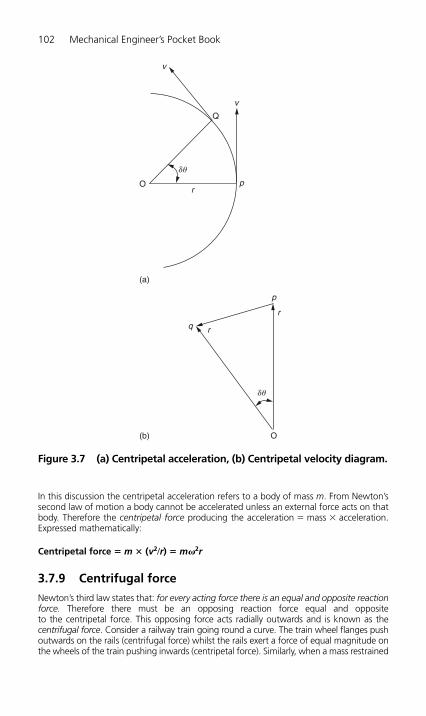
In this discussion the centripetal acceleration refers to a body of mass m. From Newton’ssecond law of motion a body cannot be accelerated unless an external force acts on thatbody. Therefore the centripetal force producing the acceleration � mass � acceleration.Expressed mathematically:
Centripetal force � m � (v2/r) � m�2r
3.7.9 Centrifugal force
Newton’s third law states that: for every acting force there is an equal and opposite reactionforce. Therefore there must be an opposing reaction force equal and opposite to the centripetal force. This opposing force acts radially outwards and is known as the centrifugal force. Consider a railway train going round a curve. The train wheel flanges pushoutwards on the rails (centrifugal force) whilst the rails exert a force of equal magnitude onthe wheels of the train pushing inwards (centripetal force). Similarly, when a mass restrained
102 Mechanical Engineer’s Pocket Book
Q
v
v
p
du
du
Or
r
r
(a)
q
O
p
(b)
Figure 3.7 (a) Centripetal acceleration, (b) Centripetal velocity diagram.
H6508-Ch03.qxd 9/12/05 4:38 PM Page 102
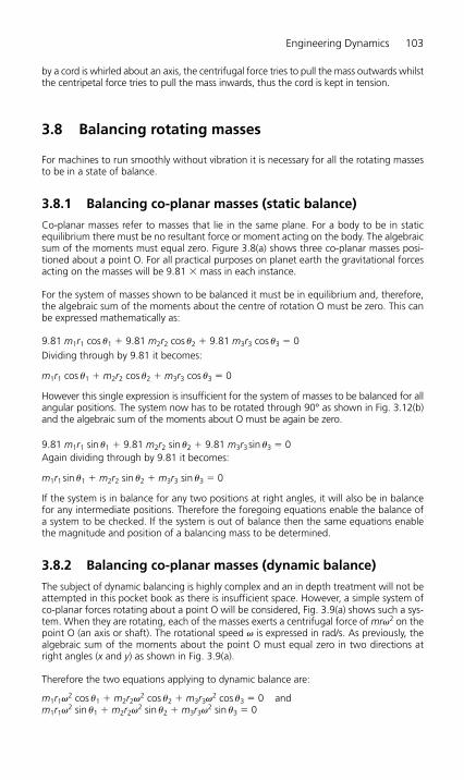
by a cord is whirled about an axis, the centrifugal force tries to pull the mass outwards whilstthe centripetal force tries to pull the mass inwards, thus the cord is kept in tension.
3.8 Balancing rotating masses
For machines to run smoothly without vibration it is necessary for all the rotating massesto be in a state of balance.
3.8.1 Balancing co-planar masses (static balance)
Co-planar masses refer to masses that lie in the same plane. For a body to be in staticequilibrium there must be no resultant force or moment acting on the body. The algebraicsum of the moments must equal zero. Figure 3.8(a) shows three co-planar masses posi-tioned about a point O. For all practical purposes on planet earth the gravitational forcesacting on the masses will be 9.81 � mass in each instance.
For the system of masses shown to be balanced it must be in equilibrium and, therefore,the algebraic sum of the moments about the centre of rotation O must be zero. This canbe expressed mathematically as:
9.81 m1r1 cos �1 � 9.81 m2r2 cos �2 � 9.81 m3r3 cos �3 � 0Dividing through by 9.81 it becomes:
m1r1 cos �1 � m2r2 cos �2 � m3r3 cos �3 � 0
However this single expression is insufficient for the system of masses to be balanced for allangular positions. The system now has to be rotated through 90° as shown in Fig. 3.12(b)and the algebraic sum of the moments about O must be again be zero.
9.81 m1r1 sin �1 � 9.81 m2r2 sin �2 � 9.81 m3r3sin �3 � 0Again dividing through by 9.81 it becomes:
m1r1sin �1 � m2r2 sin �2 � m3r3 sin �3 � 0
If the system is in balance for any two positions at right angles, it will also be in balancefor any intermediate positions. Therefore the foregoing equations enable the balance ofa system to be checked. If the system is out of balance then the same equations enablethe magnitude and position of a balancing mass to be determined.
3.8.2 Balancing co-planar masses (dynamic balance)
The subject of dynamic balancing is highly complex and an in depth treatment will not beattempted in this pocket book as there is insufficient space. However, a simple system ofco-planar forces rotating about a point O will be considered, Fig. 3.9(a) shows such a sys-tem. When they are rotating, each of the masses exerts a centrifugal force of mr�2 on thepoint O (an axis or shaft). The rotational speed � is expressed in rad/s. As previously, thealgebraic sum of the moments about the point O must equal zero in two directions atright angles (x and y) as shown in Fig. 3.9(a).
Therefore the two equations applying to dynamic balance are:
m1r1�2 cos �1 � m2r2�2 cos �2 � m3r3�2 cos �3 � 0 and m1r1�2 sin �1 � m2r2�2 sin �2 � m3r3�2 sin �3 � 0
Engineering Dynamics 103
H6508-Ch03.qxd 9/12/05 4:38 PM Page 103

104 Mechanical Engineer’s Pocket Book
c
d
m1
m2
m3
a
9.81 m2
9.81 m3
9.81 m1
O
bu1
u2
u3
r1
r2
r3
b
a
m3
m1
m2
c
9.81 m1
9.81 m2
9.81 m3
O
d
r3r1
r2
(a)
(b)
Figure 3.8 Static balance of co-planar masses. (a) Co-planar massesin first position. (b) Co-planar masses rotated through 90° to secondposition.
H6508-Ch03.qxd 9/12/05 4:38 PM Page 104
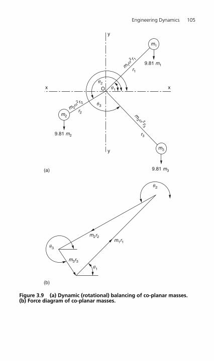
Engineering Dynamics 105
y
y
m 2ω2 r 2
m3 ω 2r
3m 1
ω2 r 1
m1
m2
m3
x
9.81 m2
9.81 m3
9.81 m1
O xu1
u2
u3
u3
u1
u2
r1
r2
r3
(a)
(b)
m3r3
m2r2m1r1
Figure 3.9 (a) Dynamic (rotational) balancing of co-planar masses.(b) Force diagram of co-planar masses.
H6508-Ch03.qxd 9/12/05 4:38 PM Page 105

Dividing through by �2, which is a constant for any given speed of rotation, the equationsbecome identical to the previous ones for static balance. Therefore for any system of co-planar forces the conditions for static and dynamic balance are the same and inde-pendent of the speed of rotation. Figure 3.9(b) shows the vector diagram of forces repre-senting the previous equations.
● If the diagram is closed as shown, then the masses are in balance.● If the diagram does not close then the masses are not in balance and the closing vec-
tor gives the angular position and the mr value of the mass required to achieve balancein the system.
3.9 Relative velocities
3.9.1 Relative velocities (unconnected bodies)
The statement that a body is travelling at 50 km/h means that the body is travelling at50 km/h relative to some other body such as the surface of planet earth. For example, anaircraft whose indicated airspeed is 300 km/h means that its airspeed is relative to thewind speed through which it is flying. The true speed of the aircraft over the ground maybe greater than its airspeed if it has a following (tail) wind, or its speed over the groundwill be less than its airspeed if it is flying into a headwind.
Figure 3.10(a) shows two unconnected bodies represented by the points P and Q. Thesebodies are travelling in opposite directions at 3 and 5 m/s, respectively. Assume that move-ment from left to right is positive and the movement from right to left is negative.
The velocity of Q relative to P � velocity Q � velocity P � (�5 m/s) � (�3 m/s) � �8 m/s
The velocity of Q relative to P is negative because the direction of Q is from right to left.Similarly:
The velocity of P relative to Q � (�3 m/s) � (�5 m/s) � �8 m/s
The velocity of P relative to Q is positive because the direction of P is from left to right. Inthis explanation the choice of direction is arbitrary. The relative directions and the alloca-tion of positive or negative values must be established at the start of each specific problem.
Since the bodies are moving in opposite directions their relative velocity is the closingvelocity. Had the two bodies been moving in the same direction as shown in Fig. 3.10(b).
The velocity of Q relative to P � �5 m/s � (�3 m/s) � �2 m/s
If the two bodies do not travel along the same path their relative velocities cannot bedetermined by simple addition or subtraction. Figure 3.10(c) shows two bodies P and Qmoving in different directions along different paths in the same plane. The velocity of P isvP and the velocity of Q is vQ.
To find the velocity of Q with respect to P it is necessary to find the apparent velocity of Qif P is stationary. To do this it is necessary to apply a velocity of �vP to both bodies asshown in Fig. 3.10(d) in order to bring P to rest. From the vector diagram 3.10(e) it can beseen that the components of the velocity of Q are its true velocity vQ and its superimposedvelocity (�vP). The resultant velocity of body B is represented by the vector QR which represents the velocity of Q relative to P. That is, the apparent movement of body Q as seen
106 Mechanical Engineer’s Pocket Book
H6508-Ch03.qxd 9/12/05 4:38 PM Page 106
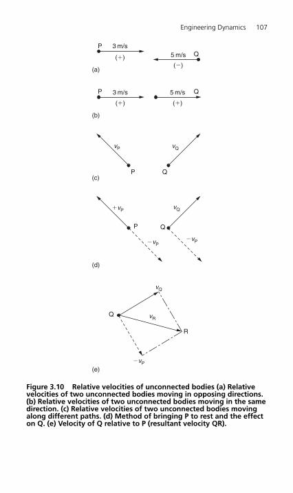
Engineering Dynamics 107
P 3 m/s5 m/s
(�)(�) Q
(a)
vQ�vP
�vP�vP
P Q
(d)
P 3 m/s 5 m/s
(�) (�)
Q
(b)
vQvP
P Q(c)
vR
vQ
�vP
(e)
R
Q
Figure 3.10 Relative velocities of unconnected bodies (a) Relativevelocities of two unconnected bodies moving in opposing directions.(b) Relative velocities of two unconnected bodies moving in the samedirection. (c) Relative velocities of two unconnected bodies movingalong different paths. (d) Method of bringing P to rest and the effecton Q. (e) Velocity of Q relative to P (resultant velocity QR).
H6508-Ch03.qxd 9/12/05 4:38 PM Page 107
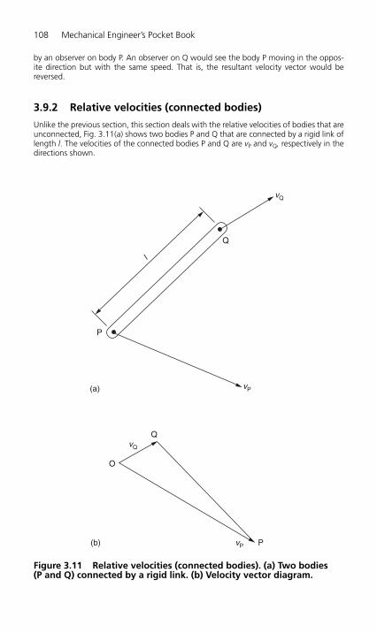
by an observer on body P. An observer on Q would see the body P moving in the oppos-ite direction but with the same speed. That is, the resultant velocity vector would bereversed.
3.9.2 Relative velocities (connected bodies)
Unlike the previous section, this section deals with the relative velocities of bodies that areunconnected, Fig. 3.11(a) shows two bodies P and Q that are connected by a rigid link oflength l. The velocities of the connected bodies P and Q are vP and vQ, respectively in thedirections shown.
108 Mechanical Engineer’s Pocket Book
Q
vQ
vP
P
vQ
Q
O
vP P
l
(a)
(b)
Figure 3.11 Relative velocities (connected bodies). (a) Two bodies (P and Q) connected by a rigid link. (b) Velocity vector diagram.
H6508-Ch03.qxd 9/12/05 4:38 PM Page 108
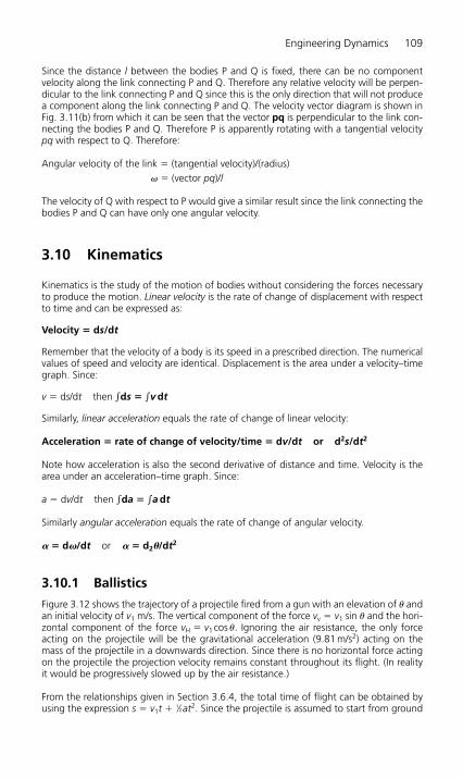
Since the distance l between the bodies P and Q is fixed, there can be no componentvelocity along the link connecting P and Q. Therefore any relative velocity will be perpen-dicular to the link connecting P and Q since this is the only direction that will not producea component along the link connecting P and Q. The velocity vector diagram is shown inFig. 3.11(b) from which it can be seen that the vector pq is perpendicular to the link con-necting the bodies P and Q. Therefore P is apparently rotating with a tangential velocitypq with respect to Q. Therefore:
Angular velocity of the link � (tangential velocity)/(radius)� � (vector pq)/l
The velocity of Q with respect to P would give a similar result since the link connecting thebodies P and Q can have only one angular velocity.
3.10 Kinematics
Kinematics is the study of the motion of bodies without considering the forces necessaryto produce the motion. Linear velocity is the rate of change of displacement with respectto time and can be expressed as:
Velocity � ds/dt
Remember that the velocity of a body is its speed in a prescribed direction. The numericalvalues of speed and velocity are identical. Displacement is the area under a velocity–timegraph. Since:
v � ds/dt then �ds � �v dt
Similarly, linear acceleration equals the rate of change of linear velocity:
Acceleration � rate of change of velocity/time � dv/dt or d2s/dt2
Note how acceleration is also the second derivative of distance and time. Velocity is thearea under an acceleration–time graph. Since:
a � dv/dt then �da � �a dt
Similarly angular acceleration equals the rate of change of angular velocity.
� � d�/dt or � � d2�/dt2
3.10.1 Ballistics
Figure 3.12 shows the trajectory of a projectile fired from a gun with an elevation of � andan initial velocity of v1 m/s. The vertical component of the force vv � v1 sin � and the hori-zontal component of the force vH � v1cos �. Ignoring the air resistance, the only forceacting on the projectile will be the gravitational acceleration (9.81 m/s2) acting on themass of the projectile in a downwards direction. Since there is no horizontal force actingon the projectile the projection velocity remains constant throughout its flight. (In realityit would be progressively slowed up by the air resistance.)
From the relationships given in Section 3.6.4, the total time of flight can be obtained byusing the expression s � v1t � 1⁄2at2. Since the projectile is assumed to start from ground
Engineering Dynamics 109
H6508-Ch03.qxd 9/12/05 4:38 PM Page 109
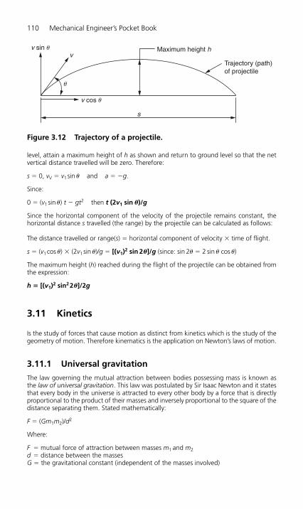
level, attain a maximum height of h as shown and return to ground level so that the netvertical distance travelled will be zero. Therefore:
s � 0, vV � v1sin � and a � �g.
Since:
0 � (v1sin �) t � gt2 then t (2v1 sin �)/g
Since the horizontal component of the velocity of the projectile remains constant, thehorizontal distance s travelled (the range) by the projectile can be calculated as follows:
The distance travelled or range(s) � horizontal component of velocity � time of flight.
s � (v1cos �) � (2v1sin �)/g � [(v1)2 sin 2�]/g (since: sin 2� � 2 sin � cos �)
The maximum height (h) reached during the flight of the projectile can be obtained fromthe expression:
h � [(v1)2 sin22�]/2g
3.11 Kinetics
Is the study of forces that cause motion as distinct from kinetics which is the study of thegeometry of motion. Therefore kinematics is the application on Newton’s laws of motion.
3.11.1 Universal gravitation
The law governing the mutual attraction between bodies possessing mass is known asthe law of universal gravitation. This law was postulated by Sir Isaac Newton and it statesthat every body in the universe is attracted to every other body by a force that is directlyproportional to the product of their masses and inversely proportional to the square of thedistance separating them. Stated mathematically:
F � (Gm1m2)/d2
Where:
F � mutual force of attraction between masses m1 and m2d � distance between the massesG � the gravitational constant (independent of the masses involved)
110 Mechanical Engineer’s Pocket Book
v sin u
u
v cos u
vMaximum height h
Trajectory (path)of projectile
s
Figure 3.12 Trajectory of a projectile.
H6508-Ch03.qxd 9/12/05 4:38 PM Page 110
For any two masses on any planet, including planet earth, the mutually attractive force Fbetween them is negligible compared with the force between each mass and the planeton which they are resting. Since planet earth exerts a force on all other bodies it followsfrom Newton’s second law of motion that this force will produce an acceleration g m/s2.Since:
(GM0M)/r � F � Mg
Therefore:
g � (GM0)/r � 9.81 m/s2
Where:
G � gravitational constant (6.668 � 10�11m3/kg s2)M0 � mass of planet earth (5.98 � 1024kg) assumed to be concentrated at the centre of
the planet.r � mean radius of planet earth (6.375 � 106m)g � mean gravitational acceleration of planet earthF � mutual force of attraction
3.11.2 Linear translation
Any body acted upon by a number of external forces so that the resultant of these forcespasses through the centre of the mass of the body then the resulting motion will be trans-latory. Further, since the resultant force acts through the centre of the mass it will have nomoment and the body will not rotate. Therefore any such motion will be translatory andwill move or tend to move the body from one place to another in a straight line.
3.11.3 Translation in a curved path
When a body moves in a curved path of radius r and at a uniform speed v it is subject toan inward radial acceleration of v2/r as discussed in Section 3.7.8. This is known as thecentripetal acceleration. Newton’s second law of motion states that a body cannot beaccelerated unless it is subjected to an external force. Thus:
Centripetal force � mass � centripetal acceleration � (mv2)/rSince v � r� for uniform circular motion, the centripetal force � m�2r
The centripetal force must be applied externally to the body for example, in the case of acar, by the friction of the tyres in contact with the road or, in the case of a railway rain bythe side-thrust of the rails on the flanges of the wheels of the rolling stock. Newton’s thirdlaw states that there is a reactive force equal and opposite to every active force. Thereforethere must be an equal and opposite force to the centripetal force. This is the centrifugalforce and it acts radially outwards. In the case of the car the car pushes outwards againstthe road surface (centrifugal force) and the road pushes back against the tyres of the car(centripetal force) unless the friction force between the tyres and the road breaks down,then the car will skid.
3.11.4 Conic pendulum
If a mass m is suspended from a pivot P by an arm of length l so that it rotates around a circular path of radius r at a constant velocity �, as shown in Fig. 3.13, then for any
Engineering Dynamics 111
H6508-Ch03.qxd 9/12/05 4:38 PM Page 111
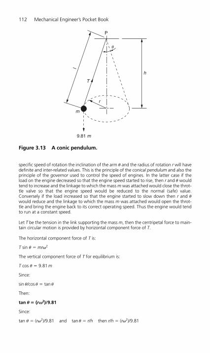
specific speed of rotation the inclination of the arm � and the radius of rotation r will havedefinite and inter-related values. This is the principle of the conical pendulum and also theprinciple of the governor used to control the speed of engines. In the latter case if theload on the engine decreased so that the engine speed started to rise, then r and � wouldtend to increase and the linkage to which the mass m was attached would close the throt-tle valve so that the engine speed would be reduced to the normal (safe) value.Conversely if the load increased so that the engine started to slow down then r and �would reduce and the linkage to which the mass m was attached would open the throt-tle and bring the engine back to its correct operating speed. Thus the engine would tendto run at a constant speed.
Let T be the tension in the link supporting the mass m, then the centripetal force to main-tain circular motion is provided by horizontal component force of T.
The horizontal component force of T is:
T sin � � mr�2
The vertical component force of T for equilibrium is:
T cos � � 9.81 m
Since:
sin �/cos � � tan �
Then:
tan � � (r�2)/9.81
Since:
tan � � (r�2)/9.81 and tan � � r/h then r/h � (r�2)/9.81
112 Mechanical Engineer’s Pocket Book
P
T
h
u
m
r
9.81 m
l
Figure 3.13 A conic pendulum.
H6508-Ch03.qxd 9/12/05 4:38 PM Page 112
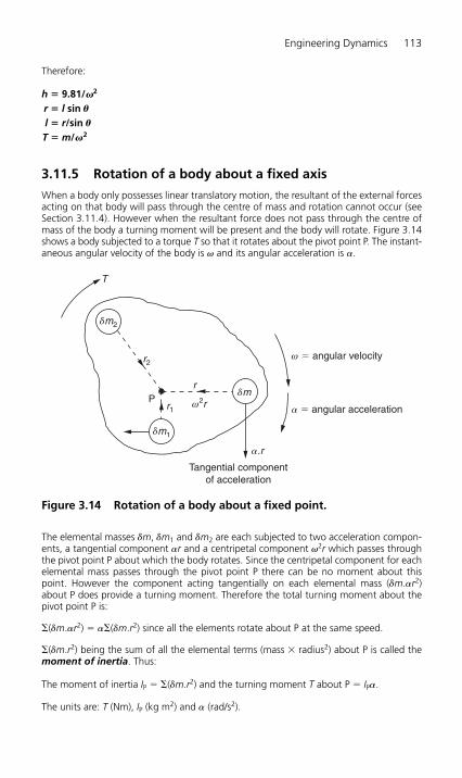
Therefore:
h � 9.81/�2
r � l sin �
l � r/sin �
T � m/�2
3.11.5 Rotation of a body about a fixed axis
When a body only possesses linear translatory motion, the resultant of the external forcesacting on that body will pass through the centre of mass and rotation cannot occur (seeSection 3.11.4). However when the resultant force does not pass through the centre ofmass of the body a turning moment will be present and the body will rotate. Figure 3.14shows a body subjected to a torque T so that it rotates about the pivot point P. The instant-aneous angular velocity of the body is � and its angular acceleration is �.
The elemental masses �m, �m1 and �m2 are each subjected to two acceleration compon-ents, a tangential component �r and a centripetal component �2r which passes throughthe pivot point P about which the body rotates. Since the centripetal component for eachelemental mass passes through the pivot point P there can be no moment about thispoint. However the component acting tangentially on each elemental mass (�m.�r2)about P does provide a turning moment. Therefore the total turning moment about thepivot point P is:
�(�m.�r2) � ��(�m.r2) since all the elements rotate about P at the same speed.
�(�m.r2) being the sum of all the elemental terms (mass � radius2) about P is called themoment of inertia. Thus:
The moment of inertia IP � �(�m.r2) and the turning moment T about P � IP�.
The units are: T (Nm), IP (kg m2) and � (rad/s2).
Engineering Dynamics 113
Tangential componentof acceleration
ω � angular velocity
a � angular acceleration
dm2
dm1
dm
T
r2
r1ω2r
a.r
rP
Figure 3.14 Rotation of a body about a fixed point.
H6508-Ch03.qxd 9/12/05 4:38 PM Page 113

3.11.6 Radius of gyration
Since the sum of the elemental masses equals the total mass of a body (m � ��m) and ifk is the distance from the chosen axis at which the total mass is assumed to be concen-trated, then mk2 � �(�m.r2) then the moment of inertia can be expressed as:
IP � mk2 where k is the radius of gyration about the specified axis of rotation.
3.11.7 Centre of percussion
It is often necessary, in rotational problems, to identify the line of action of the resultantforce F (as shown in Fig. 3.15) where F equals the mass of the body multiplied by theacceleration of the centre of mass. It is assumed that this resultant force F passes throughsome point P on the line RGP where R is the axis of rotation and G is the centre of mass.As explained in Section 3.11.6, only the tangential component of the force F can producea turning moment about R. P is at a position in a body where the moments of all theexternal forces balance out and equal zero. The point P is known as the centre ofpercussion. In cases where the body rotates about its centre of mass (R and G are coin-cident) then:
Torque T � m(kG)2� � IG�
where kG is radius of gyration about G.
When a body rotates about an axis passing through its centre of mass the radius of gyr-ation is at a minimum and, hence, the torque required to rotate the body is a minimum.
114 Mechanical Engineer’s Pocket Book
P
GF
at
atR
a � angular acceleration
ω � angular velocity
Tangential componentof F � mat
r�
l
Figure 3.15 Centre of percussion.
3.11.8 Angular momentum
It was stated in Section 3.6.8 that the linear momentum of a body was its mass multipliedby its linear velocity. The angular momentum of a rotating body is the moment of its lin-ear momentum about the point of rotation. Figure 3.16 shows a body rotating about thepivot point P with an angular velocity � rad/s. Consider the elemental mass, �m, at a dis-tance r from the pivot point P and whose velocity is v m/s.
H6508-Ch03.qxd 9/12/05 4:38 PM Page 114
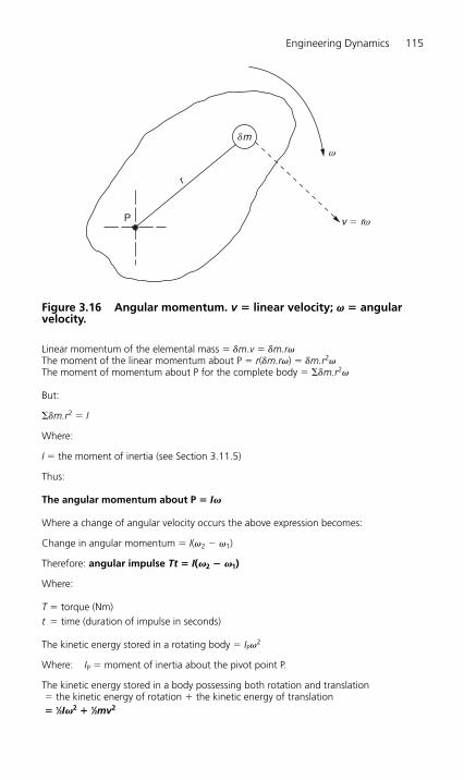
Linear momentum of the elemental mass � �m.v � �m.r�The moment of the linear momentum about P � r(�m.r�) � �m.r2�The moment of momentum about P for the complete body � ��m.r2�
But:
��m.r2 � I
Where:
I � the moment of inertia (see Section 3.11.5)
Thus:
The angular momentum about P � I�
Where a change of angular velocity occurs the above expression becomes:
Change in angular momentum � I(�2 � �1)
Therefore: angular impulse Tt � I(�2 � �1)
Where:
T � torque (Nm)t � time (duration of impulse in seconds)
The kinetic energy stored in a rotating body � IP�2
Where: IP � moment of inertia about the pivot point P.
The kinetic energy stored in a body possessing both rotation and translation� the kinetic energy of rotation � the kinetic energy of translation� 1⁄2I�2 � 1⁄2mv2
Engineering Dynamics 115
P
r
ω
dm
v � rω
Figure 3.16 Angular momentum. v � linear velocity; �� � angularvelocity.
H6508-Ch03.qxd 9/12/05 4:38 PM Page 115
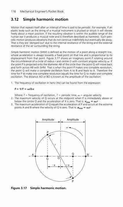
3.12 Simple harmonic motion
Motion that repeats itself after an interval of time is said to be periodic. For example, if anelastic body such as the string of a musical instrument is plucked or struck it will vibratefreely about a mean position. If the resulting vibration is within the audible range of thehuman ear it produces a musical note and is therefore described as harmonic. Such peri-odic motion produces vibrations that do not continue indefinitely but eventually die away.That is they are ‘damped out’ due to the internal resistance of the string and the externalresistance of the air surrounding the string.
Simple harmonic motion (SHM) is defined as the motion of a point along a straight line,whose acceleration is always towards a fixed point on that line and is proportional to itsdisplacement from that point. Figure 3.17 shows an imaginary point P rotating aroundthe circumference of a circle of radius r and centre O with constant angular velocity �. Ifthe point P is projected onto the diameter AB of the circle then the point Q will move backand forth across AB with SHM. That is when the point P makes one complete revolution,the point Q will make a complete oscillation from A to B and back to A. Therefore thetime for P to make one complete revolution equals the time for Q to make one completeoscillation. The distance AO or BO is known as the amplitude of the oscillation:
1. The frequency of oscillation in hertz (Hz) can be found from the expression:
f � 1/T � �/2�
Where: f � frequency of oscillation, T � periodic time, � � angular velocity.2. The maximum velocity of Q occurs at the midpoint when P is immediately above or
below the centre O and the acceleration of X is zero. That is: vmax � �.r3. The maximum acceleration of Q equals the acceleration of P and occurs at the extreme
points A and B where the velocity of Q is zero. That is: amax � �.r
116 Mechanical Engineer’s Pocket Book
Amplitude Amplitude
�x �x
A B
r
P
P
Q
Q O
ω
Figure 3.17 Simple harmonic motion.
H6508-Ch03.qxd 9/12/05 4:38 PM Page 116
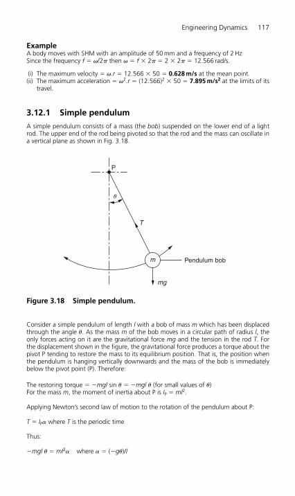
ExampleA body moves with SHM with an amplitude of 50 mm and a frequency of 2 HzSince the frequency f � �/2� then � � f � 2� � 2 � 2� � 12.566 rad/s.
(i) The maximum velocity � �.r � 12.566 � 50 � 0.628 m/s at the mean point.(ii) The maximum acceleration � �2.r � (12.566)2 � 50 � 7.895 m/s2 at the limits of its
travel.
3.12.1 Simple pendulum
A simple pendulum consists of a mass (the bob) suspended on the lower end of a lightrod. The upper end of the rod being pivoted so that the rod and the mass can oscillate ina vertical plane as shown in Fig. 3.18.
Engineering Dynamics 117
m Pendulum bob
mg
T
P
u
Figure 3.18 Simple pendulum.
Consider a simple pendulum of length l with a bob of mass m which has been displacedthrough the angle �. As the mass m of the bob moves in a circular path of radius l, theonly forces acting on it are the gravitational force mg and the tension in the rod T. For the displacement shown in the figure, the gravitational force produces a torque about thepivot P tending to restore the mass to its equilibrium position. That is, the position whenthe pendulum is hanging vertically downwards and the mass of the bob is immediatelybelow the pivot point (P). Therefore:
The restoring torque � �mgl sin � � �mgl � (for small values of �)For the mass m, the moment of inertia about P is IP � ml2.
Applying Newton’s second law of motion to the rotation of the pendulum about P:
T � IP� where T is the periodic time
Thus:
�mgl � � ml2� where � � (�g�)/l
H6508-Ch03.qxd 9/12/05 4:38 PM Page 117
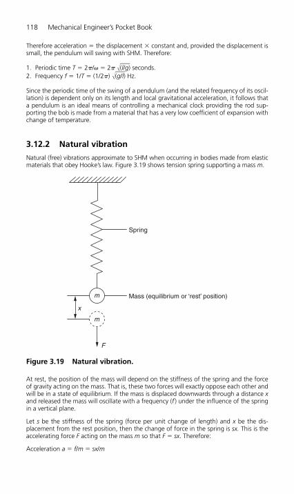
Therefore acceleration � the displacement � constant and, provided the displacement issmall, the pendulum will swing with SHM. Therefore:
1. Periodic time T � 2�/� � 2� �–––(l/g) seconds.
2. Frequency f � 1/T � (1/2�) �–––(g/l) Hz.
Since the periodic time of the swing of a pendulum (and the related frequency of its oscil-lation) is dependent only on its length and local gravitational acceleration, it follows thata pendulum is an ideal means of controlling a mechanical clock providing the rod sup-porting the bob is made from a material that has a very low coefficient of expansion withchange of temperature.
3.12.2 Natural vibration
Natural (free) vibrations approximate to SHM when occurring in bodies made from elasticmaterials that obey Hooke’s law. Figure 3.19 shows tension spring supporting a mass m.
118 Mechanical Engineer’s Pocket Book
m
m
Spring
Mass (equilibrium or ‘rest’ position)
F
x
Figure 3.19 Natural vibration.
At rest, the position of the mass will depend on the stiffness of the spring and the forceof gravity acting on the mass. That is, these two forces will exactly oppose each other andwill be in a state of equilibrium. If the mass is displaced downwards through a distance xand released the mass will oscillate with a frequency (f ) under the influence of the springin a vertical plane.
Let s be the stiffness of the spring (force per unit change of length) and x be the dis-placement from the rest position, then the change of force in the spring is sx. This is theaccelerating force F acting on the mass m so that F � sx. Therefore:
Acceleration a � f/m � sx/m
H6508-Ch03.qxd 9/12/05 4:38 PM Page 118

Therefore the acceleration is directly proportional to the displacement form the rest pos-ition of the mass m and the movement is SHM. The periodic time T of the system in seconds is given by the expression:
T � 2��––––(m/s)
The frequency f of vibration in hertz � 1/T
ExampleA load of 5 kg is hung from a tension spring so that it produces an extension of 12 mmwhen at rest. The load is displaced downwards by a further 15 mm and then release.Ignoring losses due to air resistance and hysteresis losses in the spring material determine:(i) the frequency of vibration, (ii) the maximum velocity of the load, (iii) the maximum accel-eration of the load.
(i) The weight of the load is mg � 5 kg � 9.81 m/s2 � 49.05 NThe stiffness of the spring s � force/extension � 49.05 N/15 mm � 3.27 N/mmNote: 3.27 N/mm � 3.27 kN/mThe frequency of vibration f � 1/T � 1/2� �––––
(s/m)
Therefore:
f � 1/2�� [(3.27 � 103)/5] � 4.07 Hz
(ii) The maximum velocity of the load � �x � 2�fx � 2� � 4.07 � 15 � 383.59 mm/s(iii) The maximum acceleration of the load � �2x � (2�f)2x � (2� � 4.07)2 � 15
� 9809.3 mm/s2 or 9.81 m/s2
3.13 Fluid dynamics
Hydrostatics were dealt with in Section 2.13. This section deals with fluids in motion (fluiddynamics). Fundamentally, steady uniform flow occurs when the molecules of the liquidare assumed to travel in parallel paths and the pressure and velocity of the fluid do notvary with time. Such conditions usually apply to low rates of flow in smooth-walled parallelpipes of ample cross-section.
Steady non-uniform flow occurs when the fluid is flowing through a tapered pipe. As thecross-section of the pipe becomes smaller the velocity of the fluid molecules increases sothat the same volume of fluid can pass through the reduced cross-section in a given time.However, since the velocity and pressure are constant at any particular section of pipe thiscase is still considered as steady flow, despite the fact that the flow is non-uniform alongthe length of the tapered length of pipe.
3.13.1 Rate of flow
The rate of flow or discharge of a liquid passing through a pipe can be determined fromthe following expression:
Q � Av
Engineering Dynamics 119
H6508-Ch03.qxd 9/12/05 4:38 PM Page 119

Where:
Q � rate of discharge (m3/s)A � cross-section area of pipev � velocity of flow.
Mass flow rate can be determined as follows:
�Q � �Av
Where:
� � density of the fluid�Q � mass flow rate (kg/s)
3.13.2 Continuity of flow
The above expressions refer to steady flow in pipes of uniform cross-section. For steadyflow in a tapered (converging) pipe the mass flow rate passing any given cross-section isconstant, Therefore:
�Q � �1A1v1 � �2A2v2
Where:
�Q � mass flow rateA1 and A2 � maximum and minimum cross-sectional areas (m2), respectivelyv1 � velocity of fluid flow at cross-sectional area A1 (m/s)v2 � velocity of fluid flow at cross-sectional area A2 (m/s)�1 � density of the fluid at cross-sectional area A1
�2 � density of the fluid at cross-sectional area A2
This expression is known as the equation of continuity and is applicable for all fluids bethey liquids or gasses.
For incompressible fluids (liquids) � is constant for all cross-sectional areas, therefore:
Q � A1v1 � A2v2
3.13.3 Energy of a fluid in motion (Bernoulli’s equation)
Incompressible fluids (liquids) have three forms of energy, namely:
● Potential energy: mgZ where m � mass (kg), g � 9.81 m/s2 and Z � the height of theliquid above a given datum. The potential energy per unit mass � gZ (J/kg).
● Kinetic energy: 1⁄2mv2 where: m � mass (kg) and v � uniform velocity of the liquid(m/s). The kinetic energy per unit mass � 1⁄2v2 (J/kg)
● Pressure energy: When a liquid flows through a pipe under pressure, work is done inmoving the liquid through each section of pipe against the hydrostatic pressure presentat that section. Therefore:
Work done per unit � pQ/�Q � p/� (J/kg)
120 Mechanical Engineer’s Pocket Book
H6508-Ch03.qxd 9/12/05 4:38 PM Page 120

Where: p � is the pressure, � � density of the liquid, Q � flow rate and p/� is the pres-sure energy of unit mass of the liquid.
Therefore the total energy possessed by unit mass of the liquid will be the sum of itspotential energy, its kinetic energy and its pressure energy.
Total energy per unit mass (J/kg) � gZ � v2/2 � p/�
For steady flow of an incompressible fluid (liquid) the potential, kinetic and pressure ener-gies may vary at different positions along the flow but, according to the principle of theconservation of energy the total energy will remain constant. Therefore according toBernoulli’s equation:
gZ � v2/2 � p/� � constant (K) or Z � v2/2g � p/w � constant (K)
where: w � the weight per unit volume (specific weight).
3.13.4 Flow through orifices
Water flowing from the side of a tank as a horizontal jet has only, that is, a kinetic heador a velocity head – different names for the same thing. Water stored in the tank has aninitial potential head only depending on its height h above the datum level or the meanlevel of the orifice. Therefore:
v2/2g � h v � �––––(2gh)
Since some energy is lost through friction, the jet of liquid issuing from the orifice willhave a velocity slightly less than the theoretical maximum:
Actual velocity of the jet/theoretical velocity of jet � coefficient of velocity (Cv)
The diameter of the jet of liquid issuing from the sharp-edged orifice will, in practice, beless than the actual diameter of the orifice as shown in Fig. 3.20. This is also known as thevena contracta:
Cross-section area of jet/cross-section area of orifice � coefficient of contraction (Cc)
Similarly: The actual rate of discharge/actual discharge � coefficient of discharge (Cd).Therefore:
Cd � Cv � Cc
3.13.5 Viscosity
Fluids in contact with a surface will tend to adhere to that surface. It is convenient to con-sider a fluid as having a series of layers so that the layer in contact with the surface of apipe as being at rest and the remaining layers slide over each other with gradually increas-ing velocity until the layer most remote from the surface of the pipe is moving with max-imum velocity. This is streamline flow and this condition applies when the fluid is subjectto a shear force. For example the lubricant in a bearing separating the rotating shaft fromthe bearing shell. The opposing force is the viscosity of the fluid which results in the dragexperienced when starting a vehicle engine in cold weather when the lubricant increasesin viscosity. Should the velocity increase beyond a critical value, the streamline flow breaksdown and becomes turbulent. The ‘layer’ analogy then no longer applies.
Engineering Dynamics 121
H6508-Ch03.qxd 9/12/05 4:38 PM Page 121
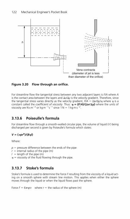
For streamline flow the tangential stress between any two adjacent layers is F/A where Ais the contact area between the layers and �v/�y is the velocity gradient. Therefore, sincethe tangential stress varies directly as the velocity gradient, F/A � (�v/�y)� where � is aconstant called the coefficient of viscosity. Thus: � (F/A)/(v/y) where the units ofviscosity are N s m�2 or kg m�1s�1 since 1 N � 1 kg m s�2.
3.13.6 Poiseulle’s formula
For streamline flow through a smooth-walled circular pipe, the volume of liquid (V ) beingdischarged per second is given by Poiseulle’s formula which states:
V � (�pr4)/(8l)
Where:
p � pressure difference between the ends of the piper � internal radius of the pipe (m)l � length of the pipe (m)� � viscosity of the fluid flowing through the pipe.
3.13.7 Stoke’s formula
Stoke’s formula is used to determine the force F resulting from the viscosity of a liquid act-ing on a smooth sphere with stream line motion. This applies when either the spheremoves through the liquid or when the liquid flows past the sphere.
Force F � 6��rv where r � the radius of the sphere (m)
122 Mechanical Engineer’s Pocket Book
Vena contracta(diameter of jet is less
than diameter of the orifice)
h
Figure 3.20 Flow through an orifice.
H6508-Ch03.qxd 9/12/05 4:38 PM Page 122
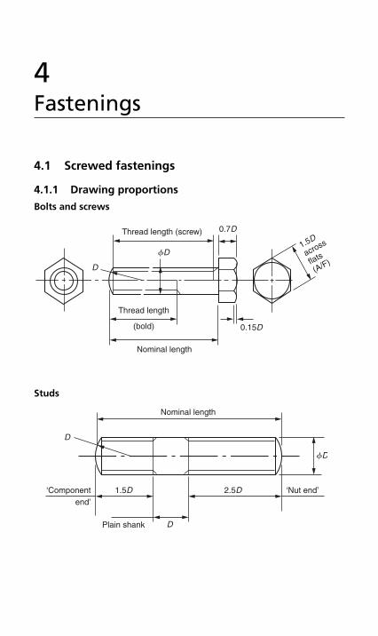
4Fastenings
4.1 Screwed fastenings
4.1.1 Drawing proportions
Bolts and screws
Studs
Thread length
Thread length (screw)
0.15D
fD
0.7D
D
1.5D
across
flats
(A/F)
(bold)
Nominal length
‘Componentend’
Plain shank
1.5D 2.5D
fD
D
D
Nominal length
‘Nut end’
H6508-Ch04.1a.qxd 9/21/05 3:13 PM Page 123
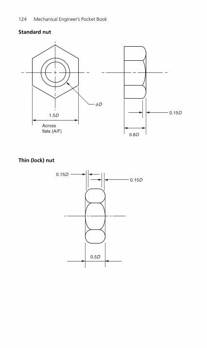
Standard nut
124 Mechanical Engineer’s Pocket Book
1.5D
Acrossflats (A/F)
fD
0.15D
0.8D
0.15D0.15D
0.5D
Thin (lock) nut
H6508-Ch04.1a.qxd 9/21/05 3:13 PM Page 124

4.1.2 Alternative screw heads
4.1.3 Alternative screw points
Fastenings 125
90° slottedcountersunk
Slottedroundhead
Slottedfillister head
Slottedinstrumenthead
Slottedhead
Phillipshead
Hexagonsockethead
Slottedcheese head
Squarehead
Flat Dog Conical Round Cup
Plain washer
f 2D
0.15D
fD
H6508-Ch04.1a.qxd 9/21/05 3:13 PM Page 125
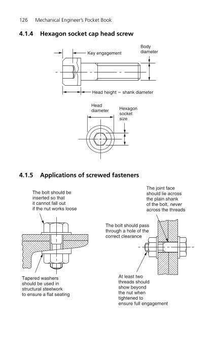
4.1.5 Applications of screwed fasteners
126 Mechanical Engineer’s Pocket Book
The bolt should beinserted so thatit cannot fall outif the nut works loose
The bolt should passthrough a hole of thecorrect clearance
At least twothreads shouldshow beyondthe nut whentightened toensure full engagement
Tapered washersshould be used instructural steelworkto ensure a flat seating
The joint faceshould lie acrossthe plain shankof the bolt, neveracross the threads
Bodydiameter
Head height � shank diameter
Hexagonsocketsize
Headdiameter
Key engagement
4.1.4 Hexagon socket cap head screw
H6508-Ch04.1a.qxd 9/21/05 3:13 PM Page 126
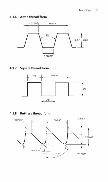
4.1.7 Square thread form
4.1.8 Buttress thread form
Fastenings 127
0.5P � 0.01
0.3707P Pitch P
0.3707P
29°
Pitch P
P/2
P/2
P/2
0.1395P
0.245PPitch P0.2754P
0.8906P
0.1205P45°7°
4.1.6 Acme thread form
H6508-Ch04.1a.qxd 9/21/05 3:13 PM Page 127
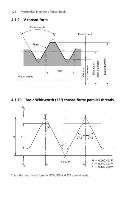
4.1.10 Basic Whitworth (55°) thread form: parallel threads
This is the basic thread form for BSW, BSF and BSP screw threads.
128 Mechanical Engineer’s Pocket Book
27.5°
H � 0.960 491Ph � 0.640 327Pr � 0.137 329P
27.5°
Pitch PHI6
HI6
h
r
r
H
Thread angle
Pitch
Flank
Axis of thread Min
or o
r
root
dia
met
er
Effe
ctiv
e or
pitc
h di
amet
er
Thread depth
Maj
or d
iam
eter
4.1.9 V-thread form
H6508-Ch04.1a.qxd 9/21/05 3:13 PM Page 128
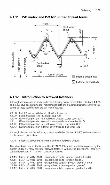
4.1.12 Introduction to screwed fasteners
Although dimensioned in ‘inch’ units the following screw thread tables (Sections 4.1.38to 4.1.43) have been retained for maintenance data and similar applications. Screwed fas-teners to these specifications are still manufactured:
4.1.38 British Standard Whitworth (BSW) bolts and nuts4.1.39 British Standard Fine (BSF) bolts and nuts4.1.40 ISO unified precision internal screw threads: coarse series (UNC)4.1.41 ISO unified precision external screw threads: coarse series (UNC)4.1.42 ISO unified precision internal screw threads: fine series (UNF)4.1.43 ISO unified precision external screw threads: fine series (UNF)
Although obsolescent the following screw thread table (Section 4.1.45) has been retainedfor the reasons given above:
4.1.45 British Association (BA) internal and external screw threads
The tables based on abstracts from the BS EN 24 000 series have been replaced by thecurrent BS EN ISO 4000 series for screwed fasteners with metric dimensions. These newstandards (Sections 4.1.13 to 4.1.21) are as follows:
4.1.13 BS EN ISO 4014: 2001 Hexagon head bolts – product grades A and B4.1.14 BS EN ISO 4016: 2001 Hexagon head bolts – product grade C4.1.15 BS EN ISO 4017: 2001 Hexagon head screws – product grades A and B4.1.16 BS EN ISO 4018: 2001 Hexagon head screws – product grade C4.1.17 BS EN ISO 4032: 2001 Hexagon nuts style 1 – product grades A and B
Fastenings 129
4.1.11 ISO metric and ISO 60° unified thread forms
0.217P
0.86
6P
0.43
3P
0.10
8P
90°
30°
60°
Root radiusof bolt
Pitc
h di
amet
er
Min
or d
iam
eter
Maj
or d
iam
eter
Axis of threadInternal thread (nut)
P/8
P/2
Pitch PRoot radiusof nut
P/4
External thread (bolt)
H6508-Ch04.1a.qxd 9/21/05 3:13 PM Page 129

4.1.18 BS EN ISO 4033: 2001 Hexagon nuts style 2 – product grades A and B4.1.19 BS EN ISO 4034: 2001 Hexagon nuts style 1 – product grade C4.1.20 BS EN ISO 4035: 2001 Hexagon thin nuts (chamfered) – product grades A and B4.1.21 BS EN ISO 4036: 2001 Hexagon thin nuts (unchamfered) – product grade B
All the above standards refer to screwed fasteners with metric dimensions that havecoarse pitch threads. Fine pitch threads will be referred to in due course.
Note:(i) BS EN ISO 4015 refers to hexagon head bolts with their shanks reduced to the effective
(pitch) diameter of their threads. These are for specialized applications and have notbeen included in this pocket book.
(ii) The mechanical property standards that were contained within BS 4190 and BS 3692can now be found in BS EN 20898 Part 1 (bolts) and Part 2 (nuts).
Interpretation of the product grade is as follows:
● Examine the table in Section 4.1.13.● The shank diameter (ds) has a maximum diameter which equals 80 mm, the nominal
diameter and also the minimum diameter.● The minimum diameter can have a product grade A tolerance or a product grade B
tolerance. The grade A tolerance is closer (more accurate) than the grade B tolerance.● Product grade A tolerances apply to fasteners with a size range from M1.6 to M24
inclusive.● Product grade B tolerances apply to fasteners with a size range from M16 to M64.● Therefore sizes M16 to M24 inclusive can have product grade A or B tolerances and the
required tolerance must be specified.● Note that the product grade is not only influenced by the diameter but also by the
length as well.
Example 1An M5 hexagon head bolt will lie within product grade A tolerances and will have a shankdiameter lying between 5.00 and 4.82 mm inclusive.
Example 2An M36 hexagon head bolt will lie within product grade B tolerances and will have ashank diameter lying between 36.00 and 35.38 mm inclusive.
Example 3An M16 hexagon head bolt will have a shank diameter lying between 16 and 15.73 mminclusive if it is to product grade A tolerances. If it is to product grade B tolerances, it willhave a shank diameter lying between 16 and 15.57 mm inclusive.
Note: The above system of tolerancing applies to all the other dimensions for the fasten-ers in these tables:
● Examine the table in Section 4.1.14. All the dimensions in this table refer to screwedfasteners with product grade C tolerances. Comparing this table with the previousexamples shows that the fasteners made to the product grade C specifications have much coarser tolerances than those manufactured to product grades A and B tolerances.
● An M12 bolt to product grade A has a shank diameter (ds) lying between 12 and11.73 mm (a tolerance of 0.27 mm), whereas an M12 bolt made product grade C willhave a shank diameter (ds) lying between 12.77 and 11.3 mm (a tolerance of 1.4 mm).Product grade B does not apply to this size of bolt.
130 Mechanical Engineer’s Pocket Book
H6508-Ch04.1a.qxd 9/21/05 3:13 PM Page 130

Fastenings 131
Note: The old terminology of ‘black’ (hot forged) and ‘bright/precision’ (cold headed or machined from hexagon bar) bolts and nuts no longer applies. However hot forged(black) bolts and nuts made to special order would only have been made to product grade C.
All the previous notes refer to hexagon head bolts, screws and nuts with coarse pitch threads. Bolts have a plain shank between the thread and the head, whereas ascrew is threaded virtually all the way up to the head. The following tables and standards(Sections 4.1.22 to 4.1.26) refer to a corresponding fine pitch series of screwed fasten-ers. These fine pitch series of screwed fasteners are only available in product grades A and B.
4.1.22 BS EN ISO 8765: 2001 Hexagon head bolts with metric fine pitch threads –product grades A and B4.1.23 BS EN ISO 8676: 2001 Hexagon head screws with metric fine pitch threads –product grades A and B4.1.24 BS EN ISO 8673: 2001 Hexagon nuts style 1 with metric fine pitch threads –product grades A and B4.1.25 BS EN ISO 8674: 2001 Hexagon nuts style 2 with metric fine pitch threads –product grades A and B4.1.26 BS EN ISO 8675: 2001 Hexagon thin nuts with metric fine pitch threads – productgrades A and B
H6508-Ch04.1a.qxd 9/21/05 3:13 PM Page 131

132 Mechanical Engineer’s Pocket Book
Example for the designation of a hexagon head bolt with thread M12, nominal lengthl � 80 mm and property class 8.8:
Hexagon head bolt ISO 4014 – M12 � 80 � 8.8
30°15°
Dimension in millimetres
Maximum underhead fillet
0.1Referee datum for dw
X
k
k'
r
r
c
g
lf
ls
d s
d a d wd e
s
l
(b)
X
u (1)
(1) Incomplete thread u � 2 P
lg
Point must be chamfered or for threads � M4may be as-rolled (sheared end)(see ISO 4753)
4.1.13 BS EN ISO 4014: 2001 Hexagon head bolts – productgrades A and B
DimensionsNote: Symbols and descriptions of dimensions are specified in ISO 225.
H6508-Ch04.1a.qxd 9/21/05 3:13 PM Page 132

M1.6
0.35
9
–
–
–
–
–
–
–
–
–
0.1
0.25
2
1.6
1.46
2.27
3.41
0.6
1.1
0.975
1.225
0.68
0.1
3.2
3.02
M2
0.4
10
–
–
–
–
–
–
–
–
–
0.1
0.25
2.6
2
1.86
3.07
4.32
0.8
1.4
1.275
1.525
0.89
0.1
4
3.82
M2.5
0.45
–
–
–
–
–
–
–
–
–
0.1
0.25
3.1
2.5
2.36
4.07
5.45
1
1.7
1.575
1.825
1.1
0.1
5
4.82
M3
0.5
12
–
–
–
–
–
–
–
–
–
0.15
0.4
3.6
3
2.86
4.57
6.01
1
2
1.875
2.125
1.31
0.1
5.5
5.32
M4
0.7
14
–
–
–
–
–
–
–
–
–
0.15
0.4
4.7
4
3.82
5.88
7.66
1.2
2.8
2.675
2.925
1.87
0.2
7
6.78
M5
0.8
16
–
–
–
–
–
–
–
–
–
0.15
0.5
5.7
5
4.82
6.88
8.79
1.2
3.5
3.35
3.65
2.35
0.2
8
7.78
M6
1
18
–
–
–
–
–
–
–
–
–
0.15
0.5
6.8
6
5.82
8.88
11.05
1.4
4
3.85
4.15
2.7
0.25
10
9.78
M8
1.25
22
–
–
–
–
–
–
–
–
–
0.15
0.6
9.2
8
7.78
11.63
14.38
2
5.3
5.15
5.45
3.61
0.4
13
12.73
M10
1.5
26
–
–
0.15
0.6
11.2
10
9.78
–
14.63
–
17.77
–
2
6.4
6.22
6.58
–
–
4.35
–
0.4
16
15.73
–
M12
1.75
30
–
–
0.15
0.6
13.7
12
11.73
–
16.63
–
20.03
–
3
7.5
7.32
7.68
–
–
5.12
–
0.6
18
17.73
–
M16
2
38
44
–
0.2
0.8
17.7
16
15.73
15.57
22.49
22
26.75
26.17
3
10
9.82
10.18
9.71
10.29
6.87
6.8
0.6
24
23.67
23.16
M20
2.5
46
52
–
0.2
0.8
22.4
20
19.67
19.48
28.19
27.7
33.53
32.95
4
12.5
12.285
12.715
12.15
12.85
8.6
8.51
0.8
30
29.67
29.16
M24
3
54
60
73
0.2
0.8
26.4
24
23.67
23.48
33.61
33.25
39.98
39.55
4
15
14.785
15.215
14.65
15.35
10.35
10.26
0.8
36
35.38
35
M30
3.5
66
72
85
0.2
0.8
33.4
30
–
29.48
–
42.75
–
50.85
6
18.7
–
–
18.28
19.12
–
12.8
1
46
–
45
M36
4
–
84
97
0.2
0.8
39.4
36
–
35.38
–
51.11
–
60.79
6
22.5
–
–
22.08
22.92
–
15.46
1
55
–
53.8
M42
4.5
–
96
109
0.3
1
45.6
42
–
41.38
–
59.95
–
71.3
8
26
–
–
25.58
26.42
–
17.91
1.2
65
–
63.1
M48
5
–
108
121
0.3
1
52.6
48
–
47.38
–
69.45
–
82.6
10
30
–
–
29.58
30.42
–
20.71
1.6
75
–
73.1
M56
5.5
–
–
137
0.3
1
63
56
–
55.26
–
78.66
–
93.56
12
35
–
–
34.5
35.5
–
24.15
2
85
–
82.8
M64
6
–
–
153
0.3
1
71
64
–
63.26
–
88.16
–
104.86
13
40
–
–
39.5
40.5
–
27.65
2
95
–
92.8
Dimensions in mmThread size, d
P a
–b
b ref. –c
–d
cmin.
max.
da max.
nom. � max.
dsProduct grade A
Bmin.
Product grade AB
min.dw
e Product grade AB
min.
lf max.
nom.
Product grade A min.max.k
Product grade B min.max.
k� e Product grade AB
min.
r min.
nom. � max.
sProduct grade A
Bmin.
BS EN ISO 4014: 2001 Table 1 Preferred threads
continued

Thread size, d M1.6 M2 M2.5 M3 M4 M5 M6 M8
Product gradeA B ls and lgf, g
lnom. min. max. min. max.
lgmax.
lsmin.
lsmin.
lgmax.
lsmin.
lgmax.
lsmin.
lgmax.
lsmin.
lgmax.
lsmin.
lgmax.
lsmin.
lgmax.
lsmin.
lgmax.
12.35 – 1.2 3
16.35 – 5.2 7 4 6 2.75 5For sizes above the stepped line, marked thus _____, ISO 4017 is recommended.
20.42 – 8 10 6.75 9 5.5 8
25.42 – 11.75 14 10.5 13 7.5 11 5 9
30.42 – 15.5 18 12.5 16 10 14 7 12
– 17.5 21 15 19 12 17
– 22.5 26 20 24 17 22 11.75
25 29 22 27 16.75
– 30 34 27 32 21.75
– 32 37 26.75
– 37 42 31.75
– 36.75
– 41.75
– 51.75
18
23
28
33
38
43
48
58
–
–
111.75
121.75
132
142
152
162
182
12
16
20
25
30
35
40
45
50
55
60
65
70
80
90
100
110
120
130
140
150
160
180
200
34.5
39.5
44.5
49.5
54.4
59.4
64.4
69.4
79.4
89.3
99.3
11.65
15.65
19.58
24.58
29.58
109.3
119.3
129.2
139.2
149.2
–
–
–
35.5
40.5
45.5
50.5
55.6
60.6
65.6
70.0
80.6
90.7
100.7
110.7
120.7
130.8
140.8
150.8
–
–
–
–
–
–
–
–
–
–
––
–
–
–
–
–
–
–
–
108.25
118.25
128
138
148
158
178
197.7 202.3
M10 M12 M16 M20 M24 M30 M36 M42 M48 M56 M64
lsmin.
lgmax.
lsmin.
lgmax.
lsmin.
lgmax.
lsmin.
lgmax.
lsmin.
lgmax.
lsmin.
lgmax.
lsmin.
lgmax.
lsmin.
lgmax.
lsmin.
lgmax.
lsmin.
lgmax.
lsmin.
lgmax.
19
24
29
34
39
44
54
64
11.5
16.5
21.5
26.5
31.5
36.5
46.5
56.5
66.5 74
11.25
16.25
21.25
26.25
31.25
41.25
51.25
61.25
71.25
81.25
20
25
30
35
40
50
60
70
80
90
17
22
32
42
52
62
72
76
86
96
106
27
32
42
52
62
72
82
86
96
106
116
21.5
31.5
41.5
51.5
61.5
65.5
75.5
85.5
95.5
115.5
135.5
34
44
54
64
74
78
88
98
108
128
148
21
31
41
51
55
65
75
85
105
125
36
46
56
66
70
80
90
100
120
140
26.5
36.5
40.5
50.5
60.5
70.5
90.5
110.5
44
54
58
68
78
88
108
128
36
46
56
76
96
56
66
76
96
116
41.5
61.5
81.5
64
84
104
47
67
72
92
Dimensions in mmBS EN ISO 4014: 2001 Table 1 Preferred threads (continued)

220 – – 222.3
240 – – 242.3
260 – – 262.6
280 – – 292.6
300 – – 302.6
320 – – 322.85
340 – – 342.85
360 – – 362.85
380 – – 382.85
400 – – 402.85
420 – – 423.15
440 – – 443.15
460 – – 463.15
480 – – 483.15
500 – –
217.7
237.7
257.4
277.4
297.4
317.15
337.15
357.15
377.15
397.15
416.85
436.85
456.85
476.85
496.85 503.15
f Ig max � Inom � b; Is min � Ig max � 5P.g Ig � minimum grip length.
Note: The popular lengths are defined in terms of lengths Is and Ig:• product grade A above the stepped line, marked thus - - - -.• product grade B below this stepped line.
132 147 117.5 135 103 123 88.5 111 74 99 55.5 83
152 167 137.5 155 123 143 108.5 131 94 119 75.5 103
157.5 175 143 163 128.5 151 114 139 95.5 123 77 107
177.5 195 163 183 148.5 171 134 159 115.5 143 97 127
197.5 215 183 203 168.5 191 154 179 135.5 163 117 147
203 223 188.5 211 174 199 155.5 183 137 167
223 243 208.5 231 194 219 175.5 203 157 187
243 263 228.5 251 214 239 195.5 223 177 207
248.5 271 234 259 215.5 243 197 227
268.5 291 254 279 235.5 263 217 247
288.5 311 274 299 255.5 283 237 267
308.5 331 294 319 275.5 303 257 287
314 339 295.5 323 277 307
334 359 315.5 343 297 327
335.5 363 317 347
aP � pitch of thread.bFor lengths Inom � 125 mm.cFor lengths 125 mm � Inom � 200 mm.dFor lengths Inom � 200 mm.ek�min � 0.7 kmin.

136M
echanical Engineer’s Pocket Book
Thread size, d M3.5 M14 M18 M22 M27 M33 M39 M45 M52 M60
P a 0.6 2 2.5 2.5 3 3.5 4 4.5 5 5.5
–b 13 34 42 50 60 – – – – –
b ref. –c – 40 48 56 66 78 90 102 116 –
–d – – – 69 79 91 103 115 129 145
cmin. 0.15 0.15 0.2 0.2 0.2 0.2 0.3 0.3 0.3 0.3
max. 0.4 0.6 0.8 0.8 0.8 0.8 1 1 1 1
da max. 4.1 15.7 20.2 24.4 30.4 36.4 42.4 48.6 56.6 67
nom. � max. 3.5 14 18 22 27 33 39 46 52 60
dsProduct grade A
Bmin.
3.32 13.73 17.73 21.67 – – – – – –
– – 17.57 21.48 26.48 32.38 38.38 44.38 51.26 59.26
dw Product grade AB
min.5.07 19.37 25.34 31.71 – – – – – –
– – 24.85 31.35 38 46.55 55.86 64.7 74.2 83.41
e Product grade AB
min.6.58 23.36 30.14 37.72 – – – – – –
– – 29.56 37.29 45.2 56.37 66.44 76.95 88.25 99.21
lf max. 1 3 3 4 6 6 6 8 10 12
nom. 2.4 8.8 11.5 14 17 21 25 28 33 38
Product grade A min.max.
2.275 8.62 11.285 13.785 – – – – – –
k 2.525 8.98 11.175 14.215 – – – – – –
Product grade A min.max.
– – 11.15 13.65 16.65 20.58 24.58 27.58 32.5 37.5
– – 11.85 14.35 17.35 21.42 25.42 28.42 33.5 38.5
k�e Product grade AB
min.1.59 6.03 7.9 9.65 – – – – – –
– – 7.81 9.56 11.66 14.41 17.21 19.31 22.75 26.25
r min. 0.1 0.6 0.6 0.8 1 1 1 1.2 1.6 2
nom. � max. 6 21 27 34 41 50 60 70 80 90
sProduct grade A
Bmin.
5.82 20.67 26.67 33.38 – – – – – –
– – 26.16 33 40 49 58.8 68.1 78.1 87.8
BS EN ISO 4014: 2001 Table 2 Non-preferred threads Dimensions in mm

Fastenings137
Product gradeA B
ls and lgf,g
l ls lg ls lg ls lg ls lg ls lg ls lg ls lg ls lg ls lg ls lgnom. min. max. min. max. min. max. min. max. min. max. min. max. min. max. min. max. min. max. min. max. min. max. min. max.
20 19.58 20.42 – – 4 7
25 24.58 25.42 – – 9 12
30 29.58 30.42 – – 14 17
35 34.5 35.5 – – 19 22
40 39.5 40.5 – – For sizes above the stepped line. marked thus ________, ISO 4017 is recommended
45 44.5 45.5 – –
50 49.5 50.5 – –
55 54.4 55.6 – –
60 59.4 60.6 – – 16 26
65 64.4 65.6 – – 21 31
70 69.4 70.6 – – 26 36 15.5 28
80 79.4 80.6 – – 36 46 25.5 38
90 89.3 90.7 – – 46 56 35.5 48 27.5 40
100 99.3 100.7 98.25 101.75 56 66 45.5 58 37.5 50 25 40
110 109.3 110.7 108.25 111.75 66 76 55.5 68 47.5 60 35 50
120 119.3 120.7 118.25 121.75 76 86 65.5 78 57.5 70 45 60
130 129.2 130.8 128 132 80 90 69.5 82 61.5 74 49 64 34.5 52
140 139.2 140.8 138 142 90 100 79.5 92 71.5 84 59 74 44.5 62
150 149.2 150.8 148 152 89.5 102 81.5 94 69 84 54.5 72 40 60
160 – – 158 162 99.5 112 91.5 104 79 94 64.5 82 50 70
180 – – 178 182 119.5 132 111.5 124 99 114 84.5 102 70 90 55.5 78
200 – – 197.7 202.3 131.5 144 119 134 104.5 122 90 110 75.6 98 59 84
220 – – 217.7 222.3 138.5 151 126 141 111.5 129 97 117 82.5 105 66 91
240 – – 237.7 242.3 146 161 131.5 149 117 137 102.5 125 86 111 67.5 95
continued
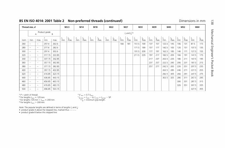
138M
echanical Engineer’s Pocket Book
Thread size, d M3.5 M14 M18 M22 M27 M33 M39 M45 M52 M60
Product gradeA B ls and lgf,g
l ls lg ls lg ls lg ls lg ls lg ls lg ls lg ls lg ls lg ls lgnom. min. max. min. max. min. max. min. max. min. max. min. max. min. max. min. max. min. max. min. max. min. max. min. max.
260 – – 257.4 262.6 166 181 151.5 169 137 157 122.5 145 106 131 87.5 115
280 – – 277.4 282.6 171.5 189 157 177 142.5 165 126 151 107.5 135
300 – – 297.4 302.6 191.5 209 177 197 162.5 185 146 171 127.5 155
320 – – 317.15 322.85 211.5 229 197 217 182.5 205 166 191 147.5 175
340 – – 337.15 342.85 217 237 202.5 225 186 211 167.5 195
360 – – 357.15 362.85 237 257 222.5 245 206 231 187.5 215
380 – – 377.15 382.85 257 277 242.5 265 226 251 207.5 235
400 – – 397.15 402.85 262.5 285 246 271 227.5 255
420 – – 416.85 423.15 282.5 305 266 291 247.5 275
440 – – 436.85 443.15 302.5 325 286 311 267.5 295
460 – – 456.85 463.15 306 331 287.5 315
480 – – 476.85 483.15 326 351 307.5 335
500 – – 496.85 503.15 327.5 355
BS EN ISO 4014: 2001 Table 2 Non-preferred threads (continued ) Dimensions in mm
a P � pitch of thread. e k�min � 0.7 kmin.b For lengths lnom � 125 mm. f lg max � lnom � b; ls min � lg max � 5P.c For lengths 125 mm � lnom � 200 mm. g lg � minimum grip length.d For lengths lnom � 200 mm.
Note: The popular lengths are defined in terms of lengths ls and lg:• product grade A above the stepped line, marked thus – – – –.• product grade B below this stepped line.

4.1.14 BS EN ISO 4016: 2001 Hexagon head bolts – productgrade C
DimensionsNote: Symbols and descriptions of dimensions are specified in ISO 225.
Example for the designation of a hexagon head bolt with thread M12, nominal lengthl � 80 mm and property class 4.6:
Hexagon head bolt ISO 4016 � M12 � 80 � 4.6
Fastenings 139
30°15°
Dimensions in millimetres
0.1Referee datum for dw
X
X
k
k'
r
c
l
(b)lg
ls
d sd a
d a d w
d
u(1)s
End withoutspecial requirements
r
Washer facepermissible
e
k
(1) Incomplete thread u � 2P.
H6508-Ch04.1a.qxd 9/21/05 3:13 PM Page 139

Thread size, d
P a
b ref.
–b
–c
–d
c max.
da max.
dsmax.
min.
dw min.
e min.
k
nom.
min.
max.
k� e min.
r min.
snom. � max.
min.
M5
0.8
16
0.5
6
5.48
4.52
6.74
8.63
3.5
3.125
3.875
2.19
0.2
8
7.64
–
–
M6
1
18
0.5
7.2
6.48
5.52
8.74
10.89
4
3.625
4.375
2.54
0.25
10
9.64
–
–
M8
1.25
22
0.6
10.2
8.58
7.42
11.47
14.2
5.3
4.925
5.675
3.45
0.4
13
12.57
–
–
M10
1.5
26
0.6
12.2
10.58
9.42
14.47
17.59
6.4
5.95
6.85
4.17
0.4
16
15.57
–
–
18
M12
1.75
30
0.6
14.7
12.7
11.3
16.47
19.85
7.5
7.05
7.95
4.94
0.6
17.57
–
–
M16
2
38
44
0.8
18.7
16.7
15.3
22
26.17
10
9.25
10.75
6.48
0.6
24
23.16
–
M20
2.5
46
52
0.8
24.4
20.84
19.16
27.7
32.95
12.5
11.6
13.4
8.12
0.8
30
29.16
–
M24
3
54
60
73
0.8
28.4
24.84
23.16
33.25
39.55
15
14.1
15.9
9.87
0.8
36
35
M30
3.5
66
72
85
0.8
35.4
30.84
29.16
42.75
50.85
18.7
17.65
19.75
12.36
1
46
45
M36
4
–
84
97
0.8
42.4
37
35
51.11
60.79
22.5
21.45
23.55
15.02
1
55
53.8
M42
4.5
–
96
109
1
48.6
43
41
59.95
71.3
26
24.95
27.05
17.47
1.2
65
63.1
M48
5
–
108
121
1
56.6
49
47
69.45
82.6
30
28.95
31.05
20.27
1.6
75
73.1
M56
5.5
–
–
137
1
67
57.2
54.8
78.66
93.56
35
33.75
36.25
23.63
2
85
82.8
M64
6
–
–
153
1
75
65.2
62.8
88.16
104.86
40
38.75
41.25
27.13
2
95
92.8
Dimensions in mmBS EN ISO 4016: 2001 Table 1 Preferred threads
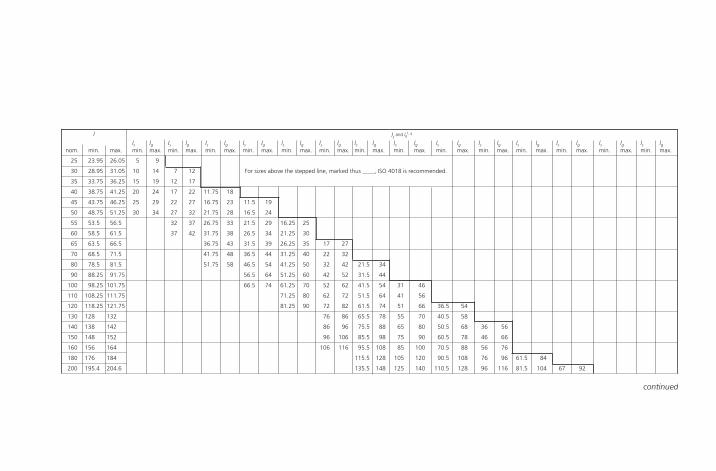
l ls and lgf, g
nom. min. max.
25 26.05 5 9
30 31.05 10 14 7 12 For sizes above the stepped line, marked thus ____, ISO 4018 is recommended.
35 36.25 15 19 12 17
40 41.25 20 24 17 22 11.75 18
45 46.25 25 29 22 27 16.75 23 11.5 19
50
23.95
28.95
33.75
38.75
43.75
48.75 51.25 30 34 27 32 21.75 28 16.5 24
55 53.5 56.5 32 37 26.75 33 21.5 29 16.25 25
60 58.5 61.5 37 42 31.75 38 26.5 34 21.25 30
65 63.5 66.5 36.75 43 31.5 39 26.25 35 17 27
70 68.5 71.5 41.75 48 36.5 44 31.25 40 22 32
80 78.5 81.5 51.75 58 46.5 54 41.25 50 32 42 21.5 34
90 88.25 91.75 56.5 64 51.25 60 42 52 31.5 44
100 98.25 101.75 66.5 74 61.25 70 52 62 41.5 54
110 108.25 111.75 71.25 80 62 72 51.5 64
120 118.25 121.75 81.25 90 72 82 61.5 74
130 128 132 76 86 65.5 78
140 138 142 86 96 75.5 88
150 148 152 96 106 85.5 98
160 156 164 106 116 95.5 108
180 176 184 115.5 128
200 195.4 204.6 135.5 148
lgmax.
lgmax.
lgmax.
lgmax.
lgmax.
lgmax.
lgmax.
lgmax.
lgmax.
lgmax.
lgmax.
lgmax.
lgmax.
lgmax.
lsmin.
lsmin.
lsmin.
lsmin.
lsmin.
lsmin.
lsmin.
lsmin.
lsmin.
lsmin.
lsmin.
lsmin.
lsmin.
lsmin.
31 46
41 56
51 66 36.5 54
55 70 40.5 58
65 80 50.5 68 36 56
75 90 60.5 78 46 66
85 100 70.5 88 56 76
105 120 90.5 108 76 96 61.5 84
125 140 110.5 128 96 116 81.5 104 67 92
continued

f lg max � lnom � b; ls min � lg max � 5P.g lg � minimum grip length.Note: The popular lengths are marked by the shank lengths.
220 215.4 224.6
240 235.4 244.6
260 254.8 265.2
280 274.8 285.2
300 294.8 305.2
320 314.3 325.7
340 334.3 345.7
360 354.3 365.7
380 374.3 385.7
400 394.3 405.7
420 413.7 426.3
440 433.7 446.3
460 453.7 466.3
480 473.7 486.3
500 493.7 506.3
a P � pitch of the thread.b For lengths lnom � 125 mm.c For lengths 125 mm � lnom � 200 mm.d For lengths lnom � 200 mm.e k�min � 0.7 kmin.
Thread size, d M5 M6 M8 M10 M12 M16 M20
l ls and lgf, g
nom. min. max.
M24 M30 M36 M42 M48 M56 M64
107
127
147
167
187
207
227
247
267
287
307
327
347
lgmax.
99
119
139
159
179
199
219
239
259
279
299
319
339
359
lgmax.
111
131
151
171
191
211
231
251
271
291
311
lgmax.
123
143
163
183
203
223
243
263
lgmax.
135
155
175
195
215
lgmax.
147
167
lgmax.
lgmax.
lgmax.
lgmax.
lgmax.
lgmax.
lgmax.
lgmax.
103
123
143
163
183
203
223
243
263
283
303
323
343
363
lgmax.
77
97
117
137
157
177
197
217
237
257
277
297
317
lsmin.
75.5
95.5
115.5
135.5
155.5
175.5
195.5
215.5
235.5
255.5
275.5
295.5
315.5
335.5
lsmin.
74
94
114
134
154
174
194
214
234
254
274
294
314
334
lsmin.
88.5
108.5
128.5
148.5
168.5
188.5
208.5
228.5
248.5
268.5
288.5
lsmin.
103
123
143
163
183
203
223
243
lsmin.
117.5
137.5
157.5
177.5
197.5
lsmin.
132
152
lsmin.
lsmin.
lsmin.
lsmin.
lsmin.
lsmin.
lsmin.
lsmin.
Dimensions in mmBS EN ISO 4016: 2001 Table 1 Preferred threads (continued)
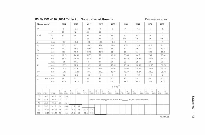
Fastenings143
Thread size, d M14 M18 M22 M27 M33 M39 M45 M52 M60
P a 2 2.5 2.5 3 3.5 4 4.5 5 5.5
–b 34 42 50 60 – – – – –
b ref –c 40 48 56 66 78 90 102 116 –
–d – – 69 79 91 103 115 129 145
c max. 0.6 0.8 0.8 0.8 0.8 1 1 1 1
da max. 16.7 21.2 26.4 32.4 38.4 45.4 52.6 62.6 71
dsmax. 14.7 18.7 22.84 27.84 34 40 46 53.2 61.2
min. 13.3 17.3 21.16 26.16 32 38 44 50.8 58.8
dw min. 19.15 24.85 31.35 38 46.55 55.86 64.7 74.2 83.41
e min. 22.78 29.56 37.29 45.2 55.37 66.44 76.95 88.25 99.21
nom. 8.8 11.5 14 17 21 25 28 33 38
k min. 8.35 10.6 13.1 16.1 19.95 23.95 26.95 31.75 36.75
max. 9.25 12.4 14.9 17.9 22.05 26.05 29.05 34.25 39.25
k�e min. 5.85 7.42 9.17 11.27 13.97 16.77 18.87 22.23 25.73
r min. 0.6 0.6 0.8 1 1 1 1.2 1.6 2
snom. � max. 21 27 34 41 50 60 70 80 90
min. 20.16 26.16 33 40 49 58.8 68.1 78.1 87.8
l ls and lgf,g
ls lg ls lg ls lg ls lg ls lg ls lg ls lg ls lg ls lgnom. min. max. min. max. min. max. min. max. min. max. min. max. min. max. min. max. min. max. min. max.
60 58.5 16 26
65 63.5 21 31 For sizes above the stepped line, marked thus ______, ISO 4018 is recommended.
70 68.5 26 36
80 78.5 36 46 25.5 38
90 88.25 46 56 35.5 48 27.5 40
100 98.25
61.5
66.5
71.5
81.5
91.75
101.75 56 66 45.5 58 37.5 50
continued
Dimensions in mmBS EN ISO 4016: 2001 Table 2 Non-preferred threads
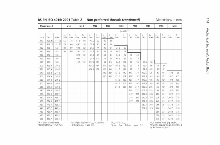
144M
echanical Engineer’s Pocket Book
l ls and lgf,g
ls lg ls lg ls lg ls lg ls lg ls lg ls lg ls lg ls lgnom. min. max. min. max. min. max. min. max. min. max. min. max. min. max. min. max. min. max. min. max.
110 108.25 111.75 66 76 55.5 68 47.5 60 35 50
120 118.25 121.75 76 86 65.5 78 57.5 70 45 60
130 128 132 80 90 69.5 82 61.5 74 49 64 34.5 52
140 138 142 90 100 79.5 92 71.5 84 59 74 44.5 62
150 148 152 89.5 102 81.5 94 69 84 54.5 72 40 60
160 156 164 99.5 112 91.5 104 79 94 64.5 82 50 70
180 176 184 119.5 132 111.5 124 99 114 84.5 102 70 90 55.5 78
200 195.4 204.6 131.5 144 119 134 104.5 122 90 110 75.5 98 59 84
220 215.4 224.6 138.5 151 126 141 111.5 129 97 117 82.5 105 66 91
240 235.4 244.6 146 161 131.5 149 117 137 102.5 125 86 111 67.5 95
260 254.8 265.2 166 181 151.5 167 137 157 122.5 145 106 131 87.5 115
280 274.8 285.2 171.5 189 157 177 142.5 165 126 151 107.5 135
300 294.8 305.2 191.5 209 177 197 162.5 185 146 171 127.5 155
320 314.3 325.7 211.5 229 197 217 182.5 205 166 191 147.5 175
340 334.3 345.7 217 237 202.5 225 186 211 167.5 195
Thread size, d M14 M18 M22 M27 M33 M39 M45 M52 M60
360 354.3 365.7 237 257 222.5 245 206 231 187.5 215
380 374.3 385.7 257 277 242.5 265 226 251 207.5 235
400 394.3 405.7 277 297 262.5 285 246 271 227.5 255
420 413.7 426.3 282.5 305 266 291 247.5 275
440 433.7 446.3 302.5 325 286 311 267.5 295
460 453.7 466.3 306 331 287.5 315
480 473.7 486.3 326 351 307.5 335
500 493.7 506.3 346 371 327.5 355
a P � pitch of the thread.b For lengths lnom � 125 mm.
c For lengths 125 mm � lnom � 200 mm.d For lengths lnom � 200 mm.
e k�min � 0.7 kmin.f lg max � lnom � b; ls min � lg max � 5P.
g lg is the minimum grip length.Note: The popular length are markedby the shank lengths.
Dimensions in mmBS EN ISO 4016: 2001 Table 2 Non-preferred threads (continued)

4.1.15 BS EN ISO 4017: 2001 Hexagon head screws – product grades A and B
DimensionsNote: Symbols and descriptions of dimensions are specified in ISO 225.
Example for the designation of a hexagon head screw with thread size M12, nominallength l � 80 mm and property class 8.8:
Hexagon head screw ISO 4017 � M12 � 80 � 8.8
Fastenings 145
30°15°
X
k
d
l
u (1)
Point must be chamfered or for threads �M4 may beas-rolled (sheared end)(see ISO 4753)
X
s
e
0.1Referee datum for dw
k'
r
c a
d ad w
a
r
d a
d s(2
)
Permissible shape
Dimensions in millimetres
(1) Incomplete thread u � 2P.(2) ds � pitch diameter.
H6508-Ch04.1a.qxd 9/21/05 3:13 PM Page 145
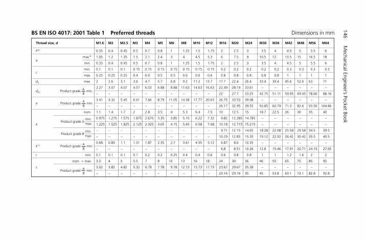
146M
echanical Engineer’s Pocket Book
Thread size, d M1.6 M2 M2.5 M3 M4 M5 M6 M8 M10 M12 M16 M20 M24 M30 M36 M42 M48 M56 M64
P a 0.35 0.4 0.45 0.5 0.7 0.8 1 1.25 1.5 1.75 2 2.5 3 3.5 4 4.5 5 5.5 6
amax.b 1.05 1.2 1.35 1.5 2.1 2.4 3 4 4.5 5.3 6 7.5 9 10.5 12 13.5 15 16.5 18
min. 0.35 0.4 0.45 0.5 0.7 0.8 1 1.25 1.5 1.75 2 2.5 3 3.5 4 4.5 5 5.5 6
cmin. 0.1 0.1 0.1 0.15 0.15 0.15 0.15 0.15 0.15 0.15 0.2 0.2 0.2 0.2 0.2 0.3 0.3 0.3 0.3
max. 0.25 0.25 0.25 0.4 0.4 0.5 0.5 0.6 0.6 0.6 0.8 0.8 0.8 0.8 0.8 1 1 1 1
da max. 2 2.6 3.1 3.6 4.7 5.7 6.8 9.2 11.2 13.7 17.7 22.4 26.4 33.4 39.4 45.6 52.6 63 71
dw Product grade AB
min.2.27 3.07 4.07 4.57 6.03 6.88 8.88 11.63 14.63 16.63 22.49 28.19 33.61 – – – – – –
– – – – – – – – – – 22 27.7 33.25 42.75 51.11 59.95 69.45 78.66 88.16
e Product grade AB
min.3.41 4.32 5.45 6.01 7.66 8.79 11.05 14.38 17.77 20.03 26.75 33.53 39.98 – – – – – –
– – – – – – – – – – 26.17 32.95 39.55 50.85 60.79 71.3 82.6 93.56 104.86
nom. 1.1 1.4 1.7 2 2.8 3.5 4 5.3 6.4 7.5 10 12.5 15 18.7 22.5 26 30 35 40
Product grade A min.max.
0.975 1.275 1.575 1.875 2.675 3.35 3.85 5.15 6.22 7.32 9.82 12.285 14.785 – – – – – –
k 1.225 1.525 1.825 2.125 2.925 3.65 4.15 5.45 6.58 7.68 10.18 12.715 15.215 – – – – – –
Product grade B min.max.
– – – – – – – – – – 9.71 12.15 14.65 18.28 22.08 25.58 29.58 34.5 39.5
– – – – – – – – – – 10.29 12.85 15.35 19.12 22.92 26.42 30.42 35.5 40.5
k� c Product grade AB
min.0.68 0.89 1.1 1.31 1.87 2.35 2.7 3.61 4.35 5.12 6.87 8.6 10.35 – – – – – –
– – – – – – – – – – 6.8 8.51 10.26 12.8 15.46 17.91 20.71 24.15 27.65
r min. 0.1 0.1 0.1 0.1 0.2 0.2 0.25 0.4 0.4 0.6 0.6 0.8 0.8 1 1 1.2 1.6 2 2
nom. � max. 3.2 4 5 5.5 7 8 10 13 16 18 24 30 36 46 55 65 75 85 95
sProduct grade A
Bmin
3.02 3.82 4.82 5.32 6.78 7.78 9.78 12.73 15.73 17.73 23.67 29.67 35.38 – – – – – –
– – – – – – – – – – 23.16 29.16 35 45 53.8 63.1 73.1 82.8 92.8
BS EN ISO 4017: 2001 Table 1 Preferred threads Dimensions in mm
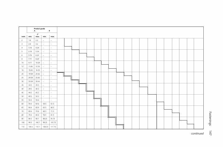
Fastenings147
Product gradeA B
ld
nom. min. max. min. max.
2 1.8 2.2 – –
3 2.8 3.2 – –
4 3.76 4.24 – –
5 4.76 5.24 – –
6 5.76 6.24 – –
8 7.71 8.29 – –
10 9.71 10.29 – –
12 11.65 12.35 – –
16 15.65 16.35 – –
20 19.58 20.42 – –
25 24.58 25.42 – –
30 29.58 30.42 – –
35 34.5 35.5 – –
40 39.5 40.5 – –
45 44.5 45.5 – –
50 49.5 50.5 – –
55 54.4 55.6 – –
60 59.4 60.6 58.5 61.5
65 64.4 65.6 63.5 66.5
70 69.4 70.6 68.5 71.5
80 79.4 80.6 78.5 81.5
90 89.3 90.7 88.25 91.75
100 99.3 100.7 98.25 101.75
110 109.3 110.7 108.25 111.75
continued

148M
echanical Engineer’s Pocket Book
Thread size, d M1.6 M2 M2.5 M3 M4 M5 M6 M8 M10 M12 M16 M20 M24 M30 M36 M42 M48 M56 M64
Product gradeA B
l d
nom. min. max. min. max.
120 119.3 120.7 118.25 121.75
130 129.2 130.8 128 132
140 139.2 140.8 138 142
150 149.2 150.8 148 152
160 – – 158 162
180 – – 178 182
200 – – 197.7 202.3
BS EN ISO 4017: 2001 Table 1 Preferred threads (continued ) Dimensions in mm
a P � pitch of the thread.b Values in accordance with a max., normal series, in ISO 3508.c k�min � 0.7 kmin.d Range of popular lengths between the stepped lines:• Product grade A above the stepped line, marked thus – – – –.• Product grade B below this stepped line.
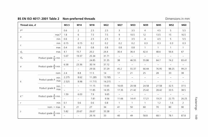
Fastenings149
Thread size, d M3.5 M14 M18 M22 M27 M33 M39 M45 M52 M60
P a 0.6 2 2.5 2.5 3 3.5 4 4.5 5 5.5
amax.b 1.8 6 7.5 7.5 9 10.5 12 13.5 15 16.5
min. 0.6 2 2.5 2.5 3 3.5 4 4.5 5 5.5
cmin. 0.15 0.15 0.2 0.2 0.2 0.2 0.3 0.3 0.3 0.3
max. 0.4 0.6 0.8 0.8 0.8 0.8 1 1 1 1
da max. 4.1 15.7 20.2 24.4 30.4 36.4 42.4 48.6 56.6 67
dw Product grade AB
min.5.07 19.37 25.34 31.71 – – – – – –
– – 24.85 31.35 38 46.55 55.86 64.7 74.2 83.41
e Product grade AB
min.6.58 23.36 30.14 37.72 – – – – – –
– – 29.56 37.29 45.2 55.37 66.44 76.95 88.25 99.21
nom. 2.4 8.8 11.5 14 17 21 25 28 33 38
Product grade A min.max.
2.275 8.62 11.285 13.785 – – – – – –
k 2.525 8.98 11.715 14.215 – – – – – –
Product grade B min.max.
– – 11.15 13.65 16.65 20.58 24.58 27.58 32.5 37.5
– – 11.85 14.35 17.35 21.42 25.42 28.42 33.5 38.5
k� c Product grade AB
min.1.59 6.03 7.9 9.65 – – – – – –
– – 7.81 9.56 11.66 14.41 17.21 19.31 22.75 26.25
r min. 0.1 0.6 0.6 0.8 1 1 1 1.2 1.6 2
nom. � max. 6 21 27 34 41 50 60 70 80 90
sProduct grade A
Bmin.
5.82 20.67 26.67 33.38 – – – – – –
– – 26.16 33 40 49 58.8 68.1 78.1 87.8
BS EN ISO 4017: 2001 Table 2 Non-preferred threads Dimensions in mm
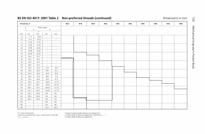
150M
echanical Engineer’s Pocket Book
Thread size, d M3.5 M14 M18 M22 M27 M33 M39 M45 M52 M60
Product gradeA B
l d
nom. min. max. min. max.
8 7.71 8.29 – –
10 9.71 10.29 – –
12 11.65 12.35 – –
16 15.65 16.35 – –
20 19.58 20.42 – –
25 24.58 25.42 – –
30 29.58 30.42 – –
35 34.5 35.5 – –
40 39.5 40.5 – –
45 44.5 45.5 – –
50 49.5 50.5 – –
55 54.4 55.6 53.5 56.5
60 59.4 60.6 58.5 61.5
65 64.4 65.6 63.5 66.5
70 69.4 70.6 68.5 71.5
80 79.4 80.6 78.5 81.5
90 89.3 90.7 88.25 91.75
100 99.3 100.7 98.25 101.75
110 109.3 110.7 108.25 111.75
120 119.3 120.7 118.25 121.75
130 129.2 130.8 128 132
140 139.2 140.8 138 142
150 149.2 150.8 148 152
160 – – 158 162
180 – – 178 182
200 – – 197.7 202.3
a P � pitch of the thread. d Range of popular lengths between the stepped lines:b Values in accordance with a max., normal series, in ISO 3508. • Product grade A above the stopped line, marked thus – – – –.c k�min � 0.7 kmin. • Product grade B below this stepped line.
BS EN ISO 4017: 2001 Table 2 Non-preferred threads (continued) Dimensions in mm
Fastenings 151
4.1.16 BS EN ISO 4018: 2001 Hexagon head screws – product grade C
DimensionsNote: Symbols and descriptions of dimensions are specified in ISO 225.
(1) Incomplete thread u � 2P.(2) ds � pitch diameter.
d a
X
k
d
l
u (1)
Y
k
s
e
k'
r
a
d a
X
rd a
d s(2)
a
Permissible shape
0.1Referee datum for dw
k'
r
c a
d ad w
Y a
r
d s(2
)
Permissible shape
30°15°
End without specialrequirements
Washer facepermissible
Dimensions in millimetres
Example for the designation of a hexagon head screw with thread M12, nominal lengthl � 80 mm and property class 4.6:
Hexagon head screw ISO 4018 – M12 � 80 � 4.6
H6508-Ch04.1b.qxd 9/21/05 3:12 PM Page 151
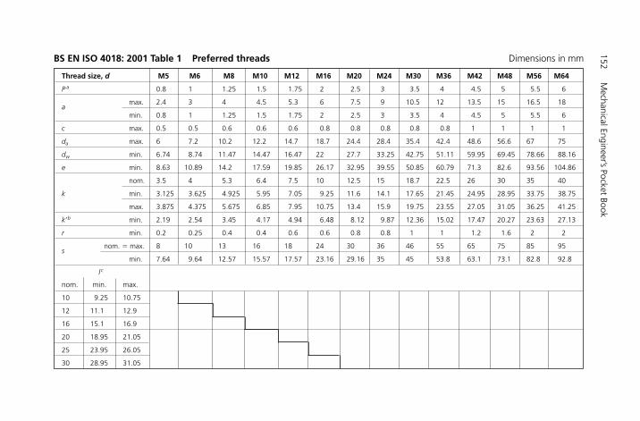
152M
echanical Engineer’s Pocket Book
Thread size, d M5 M6 M8 M10 M12 M16 M20 M24 M30 M36 M42 M48 M56 M64
P a 0.8 1 1.25 1.5 1.75 2 2.5 3 3.5 4 4.5 5 5.5 6
amax. 2.4 3 4 4.5 5.3 6 7.5 9 10.5 12 13.5 15 16.5 18
min. 0.8 1 1.25 1.5 1.75 2 2.5 3 3.5 4 4.5 5 5.5 6
c max. 0.5 0.5 0.6 0.6 0.6 0.8 0.8 0.8 0.8 0.8 1 1 1 1
da max. 6 7.2 10.2 12.2 14.7 18.7 24.4 28.4 35.4 42.4 48.6 56.6 67 75
dw min. 6.74 8.74 11.47 14.47 16.47 22 27.7 33.25 42.75 51.11 59.95 69.45 78.66 88.16
e min. 8.63 10.89 14.2 17.59 19.85 26.17 32.95 39.55 50.85 60.79 71.3 82.6 93.56 104.86
nom. 3.5 4 5.3 6.4 7.5 10 12.5 15 18.7 22.5 26 30 35 40
k min. 3.125 3.625 4.925 5.95 7.05 9.25 11.6 14.1 17.65 21.45 24.95 28.95 33.75 38.75
max. 3.875 4.375 5.675 6.85 7.95 10.75 13.4 15.9 19.75 23.55 27.05 31.05 36.25 41.25
k�b min. 2.19 2.54 3.45 4.17 4.94 6.48 8.12 9.87 12.36 15.02 17.47 20.27 23.63 27.13
r min. 0.2 0.25 0.4 0.4 0.6 0.6 0.8 0.8 1 1 1.2 1.6 2 2
snom. � max. 8 10 13 16 18 24 30 36 46 55 65 75 85 95
min. 7.64 9.64 12.57 15.57 17.57 23.16 29.16 35 45 53.8 63.1 73.1 82.8 92.8
l c
nom. min. max.
10 9.25 10.75
12 11.1 12.9
16 15.1 16.9
20 18.95 21.05
25 23.95 26.05
30 28.95 31.05
BS EN ISO 4018: 2001 Table 1 Preferred threads Dimensions in mm
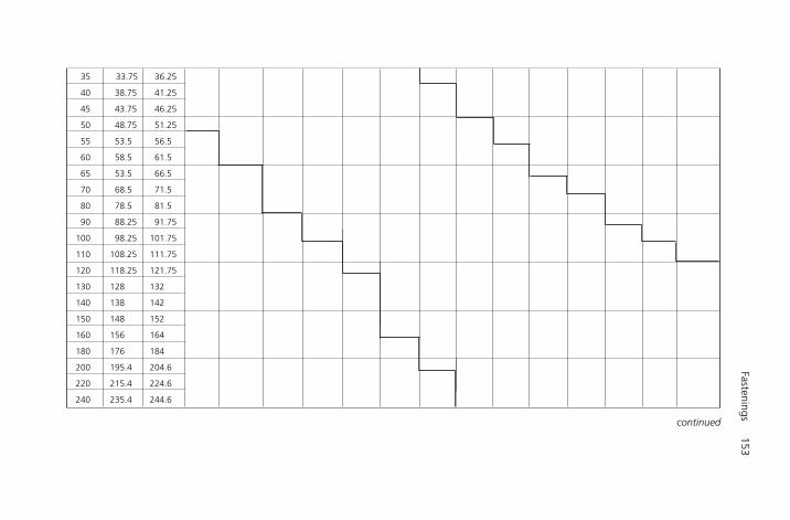
Fastenings153
35 33.75 36.25
40 38.75 41.25
45 43.75 46.25
50 48.75 51.25
55 53.5 56.5
60 58.5 61.5
65 53.5 66.5
70 68.5 71.5
80 78.5 81.5
90 88.25 91.75
100 98.25 101.75
110 108.25 111.75
120 118.25 121.75
130 128 132
140 138 142
150 148 152
160 156 164
180 176 184
200 195.4 204.6
220 215.4 224.6
240 235.4 244.6
continued

154M
echanical Engineer’s Pocket Book
Thread size, d M5 M6 M8 M10 M12 M16 M20 M24 M30 M36 M42 M48 M56 M64
260 254.8 265.2
280 274.8 285.2
300 294.8 305.2
320 314.3 325.7
340 334.3 345.7
360 354.3 365.7
380 374.3 385.7
400 394.3 405.7
420 413.7 426.3
440 433.7 446.3
460 453.7 466.3
480 473.7 486.3
500 493.7 506.3
BS EN ISO 4018: 2001 Table 1 Preferred threads (continued ) Dimensions in mm
aP � pitch of the thread.bk�min � 0.7 kmin.cRange of popular lengths between the stepped lines, marked thus –––.
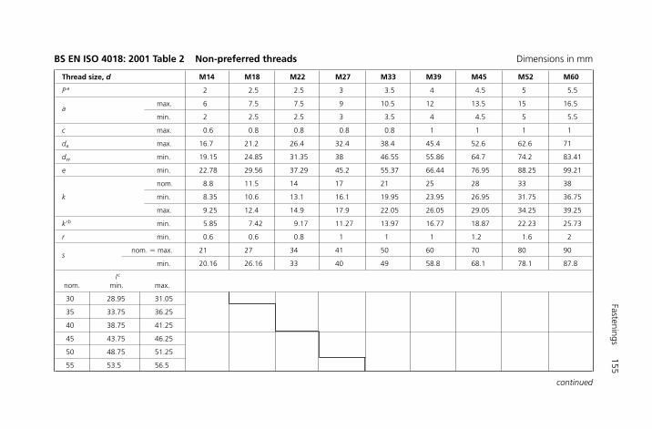
Fastenings155
Thread size, d M14 M18 M22 M27 M33 M39 M45 M52 M60
P a 2 2.5 2.5 3 3.5 4 4.5 5 5.5
amax. 6 7.5 7.5 9 10.5 12 13.5 15 16.5
min. 2 2.5 2.5 3 3.5 4 4.5 5 5.5
c max. 0.6 0.8 0.8 0.8 0.8 1 1 1 1
da max. 16.7 21.2 26.4 32.4 38.4 45.4 52.6 62.6 71
dw min. 19.15 24.85 31.35 38 46.55 55.86 64.7 74.2 83.41
e min. 22.78 29.56 37.29 45.2 55.37 66.44 76.95 88.25 99.21
nom. 8.8 11.5 14 17 21 25 28 33 38
k min. 8.35 10.6 13.1 16.1 19.95 23.95 26.95 31.75 36.75
max. 9.25 12.4 14.9 17.9 22.05 26.05 29.05 34.25 39.25
k�b min. 5.85 7.42 9.17 11.27 13.97 16.77 18.87 22.23 25.73
r min. 0.6 0.6 0.8 1 1 1 1.2 1.6 2
snom. � max. 21 27 34 41 50 60 70 80 90
min. 20.16 26.16 33 40 49 58.8 68.1 78.1 87.8
l c
nom. min. max.
30 28.95 31.05
35 33.75 36.25
40 38.75 41.25
45 43.75 46.25
50 48.75 51.25
55 53.5 56.5
continued
BS EN ISO 4018: 2001 Table 2 Non-preferred threads Dimensions in mm
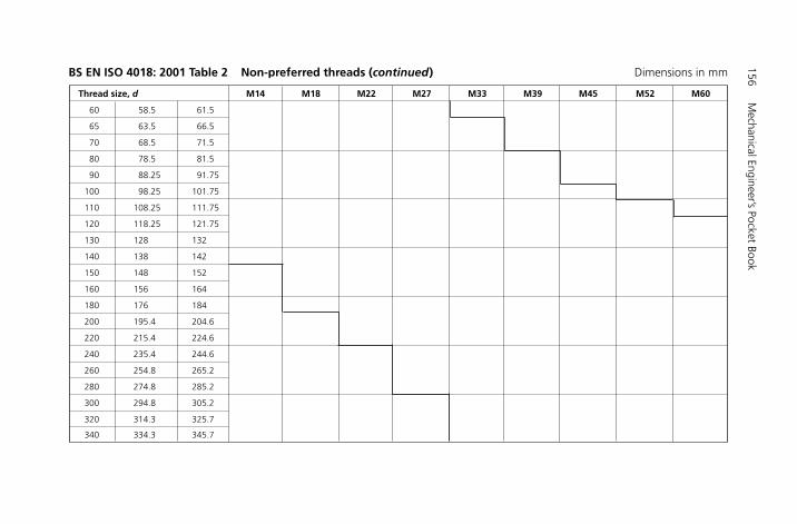
156M
echanical Engineer’s Pocket Book
Thread size, d M14 M18 M22 M27 M33 M39 M45 M52 M60
60 58.5 61.5
65 63.5 66.5
70 68.5 71.5
80 78.5 81.5
90 88.25 91.75
100 98.25 101.75
110 108.25 111.75
120 118.25 121.75
130 128 132
140 138 142
150 148 152
160 156 164
180 176 184
200 195.4 204.6
220 215.4 224.6
240 235.4 244.6
260 254.8 265.2
280 274.8 285.2
300 294.8 305.2
320 314.3 325.7
340 334.3 345.7
BS EN ISO 4018: 2001 Table 2 Non-preferred threads (continued) Dimensions in mm

Fastenings157
360 354.3 365.7
380 374.3 385.7
400 394.3 405.7
420 413.7 426.3
440 433.7 446.3
460 453.7 466.3
480 473.7 486.3
500 493.7 506.3
a P � pitch of the thread.b k�min � 0.7 kmin.c Range of popular lengths between the stepped lines, marked thus ––– .
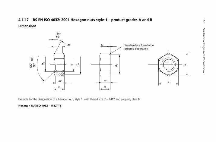
4.1.17 BS EN ISO 4032: 2001 Hexagon nuts style 1 – product grades A and B
Dimensions
158M
echanical Engineer’s Pocket Book
Washer-face form to beordered separately
120° 90
°30°
15°
d a
d wd e
m m
sm' m"
m'
ref.
C
d w
Example for the designation of a hexagon nut, style 1, with thread size d � M12 and property class 8:
Hexagon nut ISO 4032 – M12 – 8
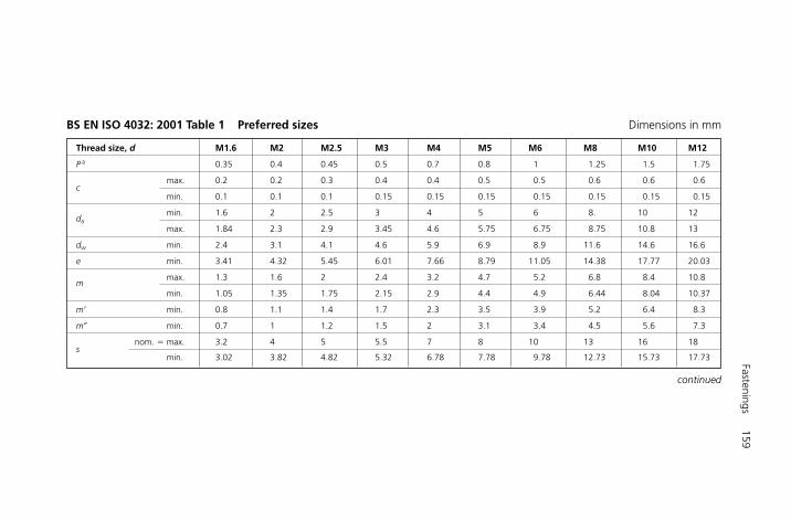
Fastenings159
Thread size, d M1.6 M2 M2.5 M3 M4 M5 M6 M8 M10 M12
P a 0.35 0.4 0.45 0.5 0.7 0.8 1 1.25 1.5 1.75
cmax. 0.2 0.2 0.3 0.4 0.4 0.5 0.5 0.6 0.6 0.6
min. 0.1 0.1 0.1 0.15 0.15 0.15 0.15 0.15 0.15 0.15
damin. 1.6 2 2.5 3 4 5 6 8. 10 12
max. 1.84 2.3 2.9 3.45 4.6 5.75 6.75 8.75 10.8 13
dw min. 2.4 3.1 4.1 4.6 5.9 6.9 8.9 11.6 14.6 16.6
e min. 3.41 4.32 5.45 6.01 7.66 8.79 11.05 14.38 17.77 20.03
mmax. 1.3 1.6 2 2.4 3.2 4.7 5.2 6.8 8.4 10.8
min. 1.05 1.35 1.75 2.15 2.9 4.4 4.9 6.44 8.04 10.37
m� min. 0.8 1.1 1.4 1.7 2.3 3.5 3.9 5.2 6.4 8.3
m� min. 0.7 1 1.2 1.5 2 3.1 3.4 4.5 5.6 7.3
snom. � max. 3.2 4 5 5.5 7 8 10 13 16 18
min. 3.02 3.82 4.82 5.32 6.78 7.78 9.78 12.73 15.73 17.73
BS EN ISO 4032: 2001 Table 1 Preferred sizes Dimensions in mm
continued

160M
echanical Engineer’s Pocket Book
Thread size, d M16 M20 M24 M30 M36 M42 M48 M56 M64
Pa 2 2.5 3 3.5 4 4.5 5 5.5 6
cmax. 0.8 0.8 0.8 0.8 0.8 1 1 1 1
min. 0.2 0.2 0.2 0.2 0.2 0.3 0.3 0.3 0.3
damin. 16 20 24 30 36 42 48 56 64
max. 17.3 21.6 25.9 32.4 38.9 45.4 51.8 60.5 69.1
dw min. 22.5 27.7 33.3 42.8 51.1 60 69.5 78.7 88.2
e min. 26.75 32.95 39.55 50.85 60.79 71.3 82.6 93.56 104.86
mmax. 14.8 18 21.5 25.6 31 34 38 45 51
min. 14.1 16.9 20.2 24.3 29.4 32.4 36.4 43.4 49.1
m� min. 11.3 13.5 16.2 19.4 23.5 25.9 29.1 34.7 39.3
m� min. 9.9 11.8 14.1 17 20.6 22.7 25.5 30.4 34.4
snom. � max. 24 30 36 46 55 65 75 85 95
min. 23.67 29.16 35 45 53.8 63.1 73.1 82.8 92.8
BS EN ISO 4032: 2001 Table 1 Preferred sizes (continued ) Dimensions in mm
aP � pitch of the thread.

Fastenings161
Thread size, d M3.5 M14 M18 M22 M27 M33 M39 M45 M52 M60
P a 0.6 2 2.5 2.5 3 3.5 4 4.5 5 5.5
cmax. 0.4 0.6 0.8 0.8 0.8 0.8 1 1 1 1
min. 0.15 0.15 0.2 0.2 0.2 0.2 0.3 0.3 0.3 0.3
da
min. 3.5 14 18 22 27 33 39 45 52 60
max. 4 15.1 19.5 23.7 29.1 35.6 42.1 48.6 56.2 64.8
dw min. 5 19.6 24.9 31.4 38 46.6 55.9 64.7 74.2 83.4
e min. 6.58 23.35 29.56 37.29 45.2 55.37 66.44 76.95 88.25 99.21
mmax. 2.8 12.8 15.8 19.4 23.8 28.7 33.4 36 42 48
min. 2.55 12.1 15.1 18.1 22.5 27.4 31.8 34.4 40.4 46.4
m� min. 2 9.7 12.1 14.5 18 21.9 25.4 27.5 32.3 37.1
m� min. 1.8 8.5 10.6 12.7 15.8 19.2 22.3 24.1 28.3 32.5
snom. � max. 6 21 27 34 41 50 60 70 80 90
min. 5.82 20.67 26.16 33 40 49 58.8 68.1 78.1 87.8
BS EN ISO 4032: 2001 Table 2 Non-preferred sizes Dimensions in mm
aP � pitch of the thread.

4.1.18 BS EN ISO 4033: 2001 Hexagon nuts style 2 – product grades A and B
Dimensions
162M
echanical Engineer’s Pocket Book
90° t
o 12
0° re
f.
15° to 30°d a d wd e
m m
sm' m'
m' c
dw
Permissiblealternativewasher-facedform
Example for the designation of a hexagon nut with metric thread size d � M12 and property class 9:
Hexagon nut ISO 4033 – M12 – 9

Fastenings163
Thread size, d M5 M6 M8 M10 M12 (M14) M16 M20 M24 M30 M36
P a 0.8 1 1.25 1.5 1.75 2 2 2.5 3 3.5 4
c max. 0.5 0.5 0.6 0.6 0.6 0.6 0.8 0.8 0.8 0.8 0.8
damin. 5 6 8 10 12 14 16 20 24 30 36
max. 5.75 6.75 8.75 10.8 13 15.1 17.3 21.6 25.9 32.4 38.9
dw min. 6.9 8.9 11.6 14.6 16.6 19.6 22.5 27.7 33.2 42.7 51.1
e min. 8.79 11.05 14.38 17.77 20.03 23.35 26.75 32.95 39.55 50.85 60.79
mmax. 5.1 5.7 7.5 9.3 12 14.1 16.4 20.3 23.9 28.6 34.7
min. 4.8 5.4 7.14 8.94 11.57 13.4 15.7 19 22.6 27.3 33.1
m� min. 3.84 4.32 5.71 7.15 9.26 10.7 12.6 15.2 18.1 21.8 26.5
smax. 8 10 13 16 18 21 24 30 36 46 55
min. 7.78 9.78 12.73 15.73 17.73 20.67 23.67 29.16 35 45 53.8
Dimensions in mm
Sizes in brackets should be avoided if possible.aP � pitch of the thread.

164 Mechanical Engineer’s Pocket Book
Nominal thread Width across diameter (mm) flats (mm)
5 8 1.08
6 10 1.44
8 13 1.23
15 0.90
10 16 1.30
17 1.73
1218 0.91
19 1.16
1421 0.96
22 1.24
16 24 1.02
20 30 0.95
24 36 0.86
30 46 1.02
36 55 1.04
BS EN ISO 4033: 2001 Table 1
Annular bearing areaThreadstress area
*
Thread size, d M10 M12 M14
P a 1.5 1.75 2
dw min. 13.6 15.6 17.4 20.4
e min. 16.64 18.90 21.10 24.49
mmax. 10 8.8 11.3 13.13
min. 9.64 8.44 10.87 12.7
m� min. 7.7 6.75 8.7 10.2
smax. 15 17 19 22
min. 14.73 16.73 18.67 21.67
BS EN ISO 4033: 2001 Table 2
* Calculation based on clearance holes ISO 273 (revised), medium series.
aP � pitch of the thread.
H6508-Ch04.1b.qxd 9/21/05 3:12 PM Page 164
Fastenings165
4.1.19 BS EN ISO 4034: 2001 Hexagon nuts style 1 – product grade C
Dimensions30°
d w d e
m
sm'
m'
15°
Countersink atstart of threadpermissible
Thread size, d M5 M6 M8 M10 M12 M16 M20
P a 0.8 1 1.25 1.5 1.75 2 2.5
dw min. 6.7 8.7 11.5 14.5 16.5 22 27.7
e min. 8.63 10.89 14.20 17.59 19.85 26.17 32.95
mmax. 5.6 6.1 7.9 9.5 12.2 15.9 19
min. 4.4 4.6 6.4 8 10.4 14.1 16.9
m� min. 3.5 3.7 5.1 6.4 8.3 11.3 13.5
snom. � max. 8 10 13 16 18 24 30
min. 7.64 9.64 12.57 15.57 17.57 23.16 29.16
BS EN ISO 4034: 2001 Table 1 Preferred sizes Dimensions in mm
Example for the designation of a hexa-gon nut with thread size d � M12 andproperty class 5:
Hexagon nut ISO 4034 – M12 – 5
continued
166M
echanical Engineer’s Pocket Book
Thread size, d M24 M30 M36 M42 M48 M56 M64
P a 3 3.5 4 4.5 5 5.5 6
dw min. 33.3 42.8 51.1 60 69.5 78.7 88.2
e min. 39.55 50.85 60.79 72.02 82.6 93.56 104.86
mmax. 22.3 26.4 31.5 34.9 38.9 45.9 52.4
min. 20.2 24.3 28 32.4 36.4 43.4 49.4
m� min. 16.2 19.5 22.4 25.9 29.1 34.7 39.5
snom.� max. 36 46 55 65 75 85 95
min. 35 45 53.8 63.1 73.1 82.8 92.8
BS EN ISO 4034: 2001 Table 1 Preferred sizes (continued ) Dimensions in mm
aP � pitch of the thread.
Thread size, d M14 M18 M22 M27 M33 M39 M45 M52 M60
P a 2 2.5 2.5 3 3.5 4 4.5 5 5.5
dw min. 19.2 24.9 31.4 38 46.6 55.9 64.7 74.2 83.4
e min. 22.78 29.56 37.29 45.2 55.37 66.44 76.95 88.25 99.21
mmax. 13.9 16.9 20.2 24.7 29.5 34.3 36.9 42.9 48.9
min. 12.1 15.1 18.1 22.6 27.4 31.8 34.4 40.4 46.4
m� min. 9.7 12.1 14.5 18.1 21.9 25.4 27.5 32.3 37.1
snom. � max. 21 27 34 41 50 60 70 80 90
min. 20.16 26.16 33 40 49 58.8 68.1 78.1 87.8
BS EN ISO 4034: 2001 Table 2 Non-preferred sizes Dimensions in mm
aP � pitch of the thread.
Fastenings167
4.1.20 BS EN ISO 4035: 2001 Hexagon thin nuts (chamfered) – product grades A and B
Dimensions
120º
ref
. 9
0º
30°15°
d a d w
d e
m
sm'
m'
Example for the designation of a chamferedthin nut with thread size d � M12 and propertyclass 05:
Hexagon thin nut ISO 4035 – M12 – 05
BS EN ISO 4035: 2001 Table 1 Preferred sizes Dimensions in mm
Thread size, d M1.6 M2 M2.5 M3 M4 M5 M6 M8 M10 M12
Pa 0.35 0.4 0.45 0.5 0.7 0.8 1 1.25 1.5 1.75
damin. 1.6 2 2.5 3 4 5 6 8 10 12
max. 1.84 2.3 2.9 3.45 4.6 5.75 6.75 8.75 10.8 13
dw min. 2.4 3.1 4.1 4.6 5.9 6.9 8.9 11.6 14.6 16.6
e min. 3.41 4.32 5.45 6.01 7.66 8.79 11.05 14.38 17.77 20.03
mmax. 1 1.2 1.6 1.8 2.2 2.7 3.2 4 5 6
min. 0.75 0.95 1.35 1.55 1.95 2.45 2.9 3.7 4.7 5.7
m� min. 0.6 0.8 1.1 1.2 1.6 2 2.3 3 3.8 4.6
snom.� max. 3.2 4 5 5.5 7 8 10 13 16 18
min. 3.02 3.82 4.82 5.32 6.78 7.78 9.78 12.73 15.73 17.73
continued
168M
echanical Engineer’s Pocket Book
BS EN ISO 4035: 2001 Table 1 Preferred sizes (continued) Dimensions in mm
Thread size, d M16 M20 M24 M30 M36 M42 M48 M56 M64
P a 2 2.5 3 3.5 4 4.5 5 5.5 6
da
min. 16 20 24 30 36 42 48 56 64
max. 17.3 21.6 25.9 32.4 38.9 45.4 51.8 60.5 69.1
dw min. 22.5 27.7 33.2 42.8 51.1 60 69.5 78.7 88.2
e min. 26.75 32.95 39.55 50.85 60.79 71.3 82.6 93.56 104.86
mmax. 8 10 12 15 18 21 24 28 32
min. 7.42 9.10 10.9 13.9 16.9 19.7 22.7 26.7 30.4
m� min. 5.9 7.3 8.7 11.1 13.5 15.8 18.2 21.4 24.3
snom.� max. 24 30 36 46 55 65 75 85 95
min. 23.67 29.16 35 45 53.8 63.1 73.1 82.8 92.8
aP � pitch of the thread.
aP � pitch of the thread.
BS EN ISO 4035: 2001 Table 2 Non-preferred sizes Dimensions in mm
Thread size, d M3.5 M14 M18 M22 M27 M33 M39 M45 M52 M60
P a 0.6 2 2.5 2.5 3 3.5 4 4.5 5 5.5
da
min. 3.5 14 18 22 27 33 39 45 52 60
max. 4 15.1 19.5 23.7 29.1 35.6 42.1 48.6 56.2 64.8
dw min. 5.1 19.6 24.9 31.4 38 46.6 55.9 64.7 74.2 83.4
e min. 6.58 23.35 29.56 37.29 45.2 55.37 66.44 76.95 88.25 99.21
mmax. 2 7 9 11 13.5 16.5 19.5 22.5 26 30
min. 1.75 6.42 8.42 9.9 12.4 15.4 18.2 21.2 24.7 28.7
m� min. 1.4 5.1 6.7 7.9 9.9 12.3 14.6 17 19.8 23
snom.� max. 6 21 27 34 41 50 60 70 80 90
min. 5.82 20.67 26.16 33 40 49 58.8 68.1 78.1 87.8
4.1.21 BS EN ISO 4036: 2001 Hexagon thin nuts (unchamfered) – product grade B
Dimensions
Example for the designation of a hexagon thin nut with metric thread d � M6 made fromsteel with HV 110 min. (st):
Hexagon nut ISO 4036 – M6-st
Fastenings 169
d
m s
Dimensions in millimetres
eBS EN ISO 4036: 2001 Table 1
Nominal thread Width across diameter (mm) flats (mm)
5 8 1.08
6 10 1.44
8 13 1.23
15 0.90
10 16 1.30
17 1.73
* Calculation based on clearance holes ISO 273 (revised), medium series.
BS EN ISO 4036: 2001 Table 2
Thread size, d M10
P a 1.5
e min. 16.46 18.73
mmax. 5 5
min. 4.52 4.52
smax. 15 17
min. 14.57 16.57
aP � pitch of the thread.
Annular bearing areaThreadstress area
*
H6508-Ch04.1b.qxd 9/21/05 3:12 PM Page 169

4.1.22 BS EN ISO 8765: 2001 Hexagon head bolts with metric fine pitch threads – product grades A and B
DimensionsNote: Symbols and descriptions of dimensions are specified in ISO 225.
170 Mechanical Engineer’s Pocket Book
30°15° Point must
be chamfered(see ISO 4753)
Dimension in millimetres
Maximum underhead fillet
(1) Incomplete thread u � 2P.
0.1Referee datum for dw
X
X
k
k'
r
r
c
l
(b )lg
lf
ls
d s
d a d wd
u (1)
e
s
H6508-Ch04.1b.qxd 9/21/05 3:12 PM Page 170
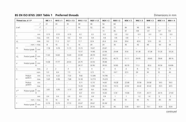
Thread size, d � P M8 � 1 M10 � 1 M12 � 1.5 M16 � 1.5 M20 � 1.5 M24 � 2 M30 � 2 M36 � 3 M42 � 3 M48 � 3 M56 � 4 M64 � 4
–a 22 26 30 38 46 54 66 – – – – –
b ref. –b – – – 44 52 60 72 84 96 108 – –
–c – – – – – 73 85 97 109 121 137 153
cmin. 0.15 0.15 0.15 0.2 0.2 0.2 0.2 0.2 0.3 0.3 0.3 0.3
max. 0.6 0.6 0.6 0.8 0.8 0.8 0.8 0.8 1 1 1 1
da max. 9.2 11.2 13.7 17.7 22.4 26.4 33.4 39.4 45.6 52.6 63 71
nom. � max. 8 10 12 16 20 24 30 36 42 48 56 64
dsProduct grade
A min.
7.78 9.78 11.73 15.73 19.67 23.67 – – – – – –
B – – – 15.57 19.48 23.48 29.48 35.8 41.38 47.38 55.26 63.26
dw Product grade A
min.11.63 14.63 16.63 22.49 28.19 33.61 – – – – – –
B – – – 22 27.7 33.25 42.75 51.11 59.95 69.45 78.66 88.16
e Product grade A
min.14.38 17.77 20.03 26.75 33.53 39.98 – – – – – –
B – – – 26.17 32.95 39.55 50.85 60.79 71.3 82.6 93.56 104.86
lf max. 2 2 3 3 4 4 6 6 8 10 12 13
nom. 5.3 6.4 7.5 10 12.5 15 18.7 22.5 26 30 35 40
Product min. 5.15 6.22 7.32 9.82 12.285 14.785 – – – – – –
kgrade A
max. 5.45 6.58 7.68 10.18 12.715 15.215 – – – – – –
Product min. – – – 9.71 12.15 14.65 18.28 22.08 25.58 29.58 34.5 39.5grade B
max. – – – 10.29 12.85 15.35 19.12 22.92 26.42 30.42 35.5 40.5
k�d Product grade A
min.3.61 4.35 5.12 6.87 8.6 10.35 – – – – – –
B – – – 6.8 8.51 10.26 12.8 15.46 17.91 20.71 24.15 27.65
r min. 0.4 0.4 0.6 0.6 0.8 0.8 1 1 1.2 1.6 2 2
nom. � max. 13 16 18 24 30 36 46 55 65 75 85 95
sProduct grade
A min.
12.73 15.73 17.73 23.67 29.67 35.38 – – – – – –
B – – – 23.16 29.16 35 45 53.8 63.1 73.1 82.8 92.8
BS EN ISO 8765: 2001 Table 1 Preferred threads Dimensions in mm
continued
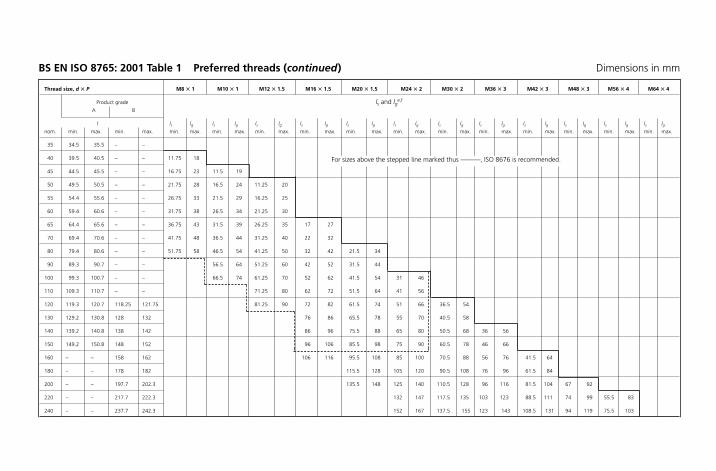
Thread size, d � P M8 � 1 M10 � 1 M12 � 1.5 M16 � 1.5 M20 � 1.5 M24 � 2 M30 � 2 M36 � 3 M42 � 3 M48 � 3 M56 � 4 M64 � 4
Product grade ls and lge,f
A B
l ls lg ls lg ls lg ls lg ls lg ls lg ls lg ls lg ls lg ls lg ls lg ls lgnom. min. max. min. max. min. max. min. max. min. max. min. max. min. max. min. max. min. max. min. max. min. max. min. max. min. max. min. max.
35 34.5 35.5 – –
40 39.5 40.5 – – 11.75 18
45 44.5 45.5 – – 16.75 23 11.5 19
50 49.5 50.5 – – 21.75 28 16.5 24 11.25 20
55 54.4 55.6 – – 26.75 33 21.5 29 16.25 25
60 59.4 60.6 – – 31.75 38 26.5 34 21.25 30
65 64.4 65.6 – – 36.75 43 31.5 39 26.25 35 17 27
70 69.4 70.6 – – 41.75 48 36.5 44 31.25 40 22 32
80 79.4 80.6 – – 51.75 58 46.5 54 41.25 50 32 42 21.5 34
90 89.3 90.7 – – 56.5 64 51.25 60 42 52 31.5 44
100 99.3 100.7 – – 66.5 74 61.25 70 52 62 41.5 54 31 46
110 109.3 110.7 – – 71.25 80 62 72 51.5 64 41 56
120 119.3 120.7 118.25 121.75 81.25 90 72 82 61.5 74 51 66 36.5 54
130 129.2 130.8 128 132 76 86 65.5 78 55 70 40.5 58
140 139.2 140.8 138 142 86 96 75.5 88 65 80 50.5 68 36 56
150 149.2 150.8 148 152 96 106 85.5 98 75 90 60.5 78 46 66
160 – – 158 162 106 116 95.5 108 85 100 70.5 88 56 76 41.5 64
180 – – 178 182 115.5 128 105 120 90.5 108 76 96 61.5 84
200 – – 197.7 202.3 135.5 148 125 140 110.5 128 96 116 81.5 104 67 92
220 – – 217.7 222.3 132 147 117.5 135 103 123 88.5 111 74 99 55.5 83
240 – – 237.7 242.3 152 167 137.5 155 123 143 108.5 131 94 119 75.5 103
BS EN ISO 8765: 2001 Table 1 Preferred threads (continued) Dimensions in mm
For sizes above the stepped line marked thus ———, ISO 8676 is recommended.

260 – – 257.4 262.6 157.5 175 143 163 128.5 151 114 139 95.5 123 77 107
280 – – 277.4 282.6 177.5 195 163 183 148.5 171 134 159 115.5 143 97 127
300 – – 297.4 302.6 197.5 215 183 203 168.5 191 154 179 135.5 163 117 147
320 – – 317.15 322.85 203 223 188.5 211 174 199 155.5 183 137 167
340 – – 337.15 342.85 223 243 208.5 231 194 219 175.5 203 157 187
360 – – 357.15 362.85 243 263 228.5 251 214 239 195.9 223 177 207
380 – – 377.15 382.85 248.5 271 234 259 215.5 243 197 227
400 – – 397.15 402.85 268.5 291 254 279 235.5 263 217 247
420 – – 416.85 423.15 288.5 311 274 299 255.5 283 237 267
440 – – 436.85 443.15 308.5 331 294 319 275.5 303 257 287
460 – – 456.85 463.15 314 339 295.5 323 277 307
480 – – 476.85 483.15 334 359 315.5 343 297 327
500 – – 496.85 503.15 335.5 363 317 347
aFor lengths lnom � 125 mm.bFor lengths 125 mm � lnom � 200 mm.cFor lengths lnom � 200 mm.dk�min � 0.7 kmin.e lg max � lnom � b; ls min � lg max � 5P.P � pitch of the coarse thread, specified in ISO 261.
f lg � the minimum grip length.
Notes:• The popular lengths are defined in terms of lengths ls and lg:
– product grade A above the stepped line, marked thus – – – – –.– product grade B below this stepped line.
• Thread sizes M10 �1 and M12 �1.5 are popular sizes but not included in ISO 262.

Thread size, d � P M10 � 1.25 M12 � 1.25 M14 � 1.5 M18 � 1.5 M20 � 2 M22 � 1.5 M27 � 2 M33 � 2 M39 � 3 M45 � 3 M52 � 4 M60 � 4
–a 26 30 34 42 46 50 60 – – – – –
b ref. –b – – 40 48 52 56 66 78 90 102 116 –
–c – – – – – 69 79 91 103 115 129 145
cmin. 0.15 0.15 0.15 0.2 0.2 0.2 0.2 0.2 0.3 0.3 0.3 0.3
max. 0.6 0.6 0.6 0.8 0.8 0.8 0.8 0.8 1 1 1 1
da max. 11.2 13.7 15.7 20.2 22.4 24.4 30.4 36.4 42.4 48.6 56.6 67
nom. � max. 10 12 14 18 20 22 27 33 39 45 52 60
dsProduct grade
A min.
9.78 11.73 13.73 17.73 19.67 21.67 – – – – – –
B – – – 17.57 19.48 21.48 26.48 32.38 38.38 44.38 51.26 59.26
dw Product grade A
min.14.63 16.63 19.37 25.34 28.19 31.71 – – – – – –
B – – – 24.85 27.7 31.35 38 46.55 55.86 64.7 74.2 83.41
e Product grade A
min.17.77 20.03 23.36 30.14 33.53 37.72 – – – – – –
B – – – 29.56 32.95 37.29 45.2 55.37 66.44 76.95 88.25 99.21
lf max. 2 3 3 3 4 4 6 6 6 8 10 12
nom. 6.4 7.5 8.8 11.5 12.5 14 17 21 25 28 33 38
Product min. 6.22 7.32 8.62 11.285 12.285 13.785 – – – – –
k grade A max. 6.58 7.68 8.98 11.715 12.715 14.215 – – – – – –
Product min. – – – 11.15 12.15 13.65 16.65 20.58 24.58 27.58 32.5 37.5grade B
max. – – – 11.85 12.85 14.35 17.35 21.42 25.42 28.42 33.5 38.5
k�d Product grade A
min.4.35 5.12 6.03 7.9 8.6 9.65 – – – – – –
B – – – 7.81 8.51 9.56 11.66 14.41 17.21 1 9.31 22.75 26.25
r min. 0.4 0.6 0.6 0.6 0.8 0.8 1 1 1. 1.2 1.6 2
nom. � max. 16 18 21 27 30 34 41 50 60 70 80 90
sProduct grade
A min.
15.73 17.73 20.67 26.67 29.67 33.38 – – – – – –
B – – – 26.16 29.16 33 40 49 58.8 68.1 78.1 87.8
BS EN ISO 8765: 2001 Table 2 Non-preferred threads Dimensions in mm
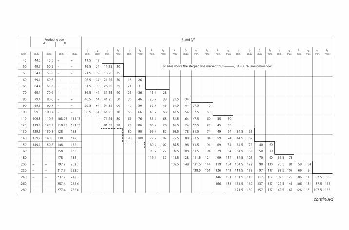
Product grade ls and lge,f
A B
l ls lg ls lg ls lg ls lg ls lg ls lg ls lg ls lg ls lg ls lg ls lg ls lgnom. min. max. min. max. min. max. min. max. min. max. min. max. min. max. min. max. min. max. min. max. min. max. min. max. min. max. min. max.
45 44.5 45.5 – – 11.5 19
50 49.5 50.5 – – 16.5 24 11.25 20
55 54.4 55.6 – – 21.5 29 16.25 25
60 59.4 60.6 – – 26.5 34 21.25 30 16 26
65 64.4 65.6 – – 31.5 39 26.25 35 21 31
70 69.4 70.6 – – 36.5 44 31.25 40 26 36 15.5 28
80 79.4 80.6 – – 46.5 54 41.25 50 36 46 25.5 38 21.5 34
90 89.3 90.7 – – 56.5 64 51.25 60 46 56 35.5 48 31.5 44 27.5 40
100 99.3 100.7 – – 66.5 74 61.25 70 56 66 45.5 58 41.5 54 37.5 50
110 109.3 110.7 108.25 111.75 71.25 80 66 76 55.5 68 51.5 64 47.5 60 35 50
120 119.3 120.7 118.25 121.75 81.25 90 76 86 65.5 78 61.5 74 57.5 70 45 60
130 129.2 130.8 128 132 80 90 69.5 82 65.5 78 61.5 74 49 64 34.5 52
140 139.2 140.8 138 142 90 100 79.5 92 75.5 88 71.5 84 59 74 44.5 62
150 149.2 150.8 148 152 89.5 102 85.5 98 81.5 94 69 84 54.5 72 40 60
160 – – 158 162 99.5 122 95.5 108 91.5 104 79 94 64.5 82 50 70
180 – – 178 182 119.5 132 115.5 128 111.5 124 99 114 84.5 102 70 90 55.5 78
200 – – 197.7 202.3 135.5 148 131.5 144 119 134 104.5 122 90 110 75.5 98 59 84
220 – – 217.7 222.3 138.5 151 126 141 111.5 129 97 117 82.5 105 66 91
240 – – 237.7 242.3 146 161 131.5 149 117 137 102.5 125 86 111 67.5 95
260 – – 257.4 262.6 166 181 151.5 169 137 157 122.5 145 106 131 87.5 115
280 – – 277.4 282.6 171.5 189 157 177 142.5 165 126 151 107.5 135
For sizes above the stepped line marked thus ———, ISO 8676 is recommended.
continued

Thread size, d � P M10 � 1.25 M12 � 1.25 M14 � 1.5 M18 � 1.5 M20 � 2 M22 � 1.5 M27 � 2 M33 � 2 M39 � 3 M45 � 3 M52 � 4 M60 � 4
Product gradeA B
l ls lg ls lg ls lg ls lg ls lg ls lg ls lg ls lg ls lg ls lg ls lg ls lgnom. min. max. min. max. min. max. min. max. min. max. min. max. min. max. min. max. min. max. min. max. min. max. min. max. min. max. min. max.
300 – – 297.4 302.6 191.5 209 177 197 162.5 185 146 171 127.5 155
320 – – 317.15 322.85 211.5 229 197 217 182.5 205 166 191 147.5 175
340 – – 337.15 342.85 217 237 202.5 225 186 211 167.5 195
360 – – 357.15 362.85 237 257 222.5 245 206 231 187.5 215
380 – – 377.15 382.85 257 277 242.5 265 226 251 207.5 235
400 – – 397.15 402.85 262.5 285 246 271 227.5 255
420 – – 416.85 423.15 282.5 305 266 291 247.5 275
440 – – 436.85 443.15 302.5 325 286 311 267.5 295
460 – – 456.85 463.15 306 331 287.5 315
480 – – 476.85 483.15 326 351 307.5 335
500 – – 496.85 503.15 327.5 355
ls and lge,f
BS EN ISO 8765: 2001 Table 2 Non-preferred threads (continued ) Dimensions in mm
aFor lengths lnom � 125 mm.bFor lengths 125 mm � lnom � 200 mm.cFor lengths lnom � 200 mm.dk�min � 0.7 kmin.e lg max � lnom � b; ls min � lg max � 5P.P � pitch of the coarse thread, specified in ISO 261.f lg is the minimum grip length.
Notes: The popular lengths are defined in terms of lengths ls and lg:• product grade A above the stepped line, marked thus – – – – –.• product grade B below this stepped line.
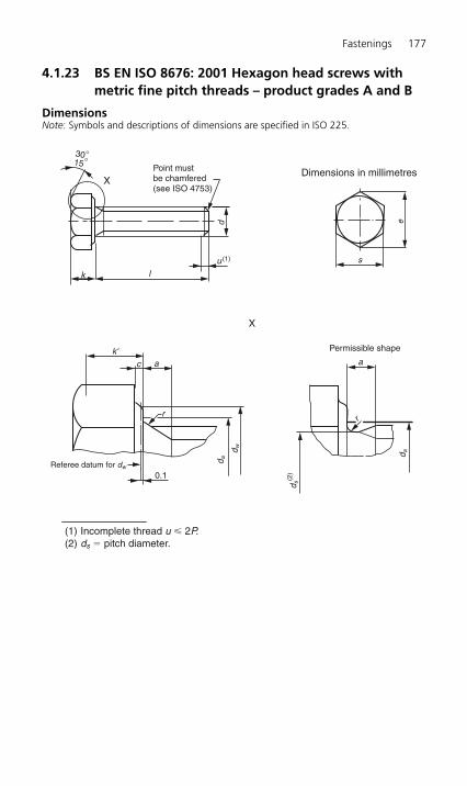
Fastenings 177
4.1.23 BS EN ISO 8676: 2001 Hexagon head screws withmetric fine pitch threads – product grades A and B
DimensionsNote: Symbols and descriptions of dimensions are specified in ISO 225.
X
k
d
l
u (1)
30°15°
X
s
e
0.1Referee datum for dw
k'
r
c a
d a
d ad w
a
r
d s(2
)
Point mustbe chamfered(see ISO 4753)
Permissible shape
Dimensions in millimetres
(1) Incomplete thread u � 2P.(2) ds � pitch diameter.
H6508-Ch04.1c.qxd 9/12/05 4:43 PM Page 177

178M
echanical Engineer’s Pocket Book
Thread size, d � P M8 � 1 M10 � 1 M12 � 1.5 M16 � 1.5 M20 � 1.5 M24 � 2 M30 � 2 M36 � 3 M42 � 3 M48 � 3 M56 � 4 M64 � 4
amax. 3 3 4.5 4.5 6 6 6 9 9 9 12 12
min. 1 1 1.5 1.5 2 2 2 3 3 3 4 4
cmin. 0.15 0.15 0.15 0.2 0.2 0.2 0.2 0.2 0.3 0.3 0.3 0.3
max. 0.6 0.6 0.6 0.8 0.8 0.8 0.8 0.8 1 1 1 1
da max. 9.2 11.2 13.7 17.7 22.4 26.4 33.4 39.4 45.6 52.6 63 71
dw Product grade A–B min.11.63 14.63 16.63 22.49 28.19 33.61 – – – – – –
– – – 22 27.7 33.25 42.75 51.11 59.95 69.45 78.66 88.16
e Product grade A–B min.14.38 17.77 20.03 26.75 33.53 39.98 – – – – – –
– – – 26.17 32.95 39.55 50.85 60.79 71.3 82.6 93.56 104.86
nom. 5.3 6.4 7.5 10 12.5 15 18.7 22.5 26 30 35 40
kProduct min. 5.15 6.22 7.32 9.82 12.285 14.785 – – – – – –
grade A max. 5.45 6.58 7.68 10.18 12.715 15.215 – – – – – –
Product min. – – – 9.71 12.15 14.65 18.28 22.08 25.58 29.58 34.5 39.5
grade B max. – – – 10.29 12.85 15.35 19.12 22.92 26.42 30.42 35.5 40.5
k�a Product grade A–B min.3.61 4.35 5.12 6.87 8.6 10.35 – – – – – –
– – – 6.8 8.51 10.26 12.8 15.46 17.91 20.71 24.15 27.65
r min. 0.4 0.4 0.6 0.6 0.8 0.8 1 1 1.2 1.6 2 2
nom. � max. 13 16 18 24 30 36 46 55 65 75 85 95s
Product grade A–B min.12.73 15.73 17.73 23.67 29.67 35.38 – – – – – –
– – – 23.16 29.16 35 45 53.8 63.1 73.1 82.8 92.8
BS EN ISO 8676: 2001 Table 1 Preferred threads Dimensions in mm
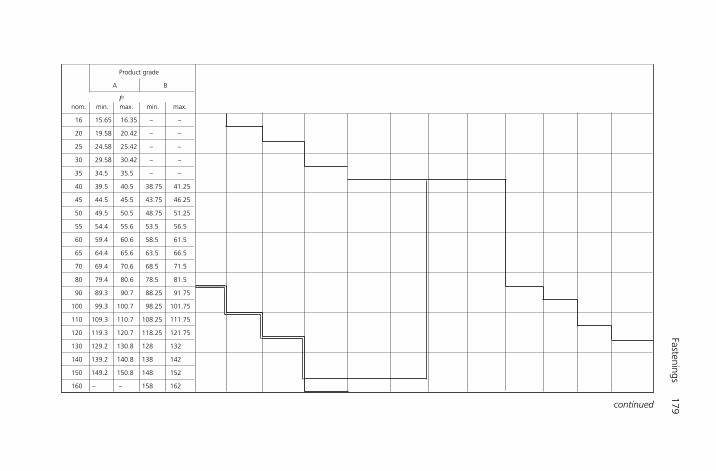
Fastenings179
Product grade
A B
lb
nom. min. max. min. max.
16 15.65 16.35 – –
20 19.58 20.42 – –
25 24.58 25.42 – –
30 29.58 30.42 – –
35 34.5 35.5 – –
40 39.5 40.5 38.75 41.25
45 44.5 45.5 43.75 46.25
50 49.5 50.5 48.75 51.25
55 54.4 55.6 53.5 56.5
60 59.4 60.6 58.5 61.5
65 64.4 65.6 63.5 66.5
70 69.4 70.6 68.5 71.5
80 79.4 80.6 78.5 81.5
90 89.3 90.7 88.25 91.75
100 99.3 100.7 98.25 101.75
110 109.3 110.7 108.25 111.75
120 119.3 120.7 118.25 121.75
130 129.2 130.8 128 132
140 139.2 140.8 138 142
150 149.2 150.8 148 152
160 – – 158 162
continued

180M
echanical Engineer’s Pocket Book
180 – – 178 182
200 – – 197.7 202.3
220 – – 217.7 222.3
240 – – 237.7 242.3
260 – – 257.4 262.6
280 – – 277.4 282.6
300 – – 297.4 302.6
320 – – 317.15 322.85
340 – – 337.15 342.85
360 – – 357.15 362.85
380 – – 377.15 382.85
400 – – 397.15 402.85
420 – – 416.85 423.15
440 – – 436.85 443.15
460 – – 456.85 463.15
480 – – 476.85 483.15
500 – – 496.85 503.15
a k�min � 0.7 kmin.b Range of popular lengths between the stepped line, marked thus –––.
• Product grade A above the stepped line, marked thus – – – – –.• Product grade B below this stepped line.
Note: The threads M10 � 1 and M12 � 1.5 are popular ones but are not included in ISO 262.
Product grade
A B
lb
nom. min. max. min. max.
BS EN ISO 8676: 2001 Table 1 Preferred threads (continued ) Dimensions in mm

Fastenings181
Thread size, d � P M10 � 1.25 M12 � 1.25 M14 � 1.5 M18 � 1.5 M20 � 2 M22 � 1.5 M27 � 2 M33 � 2 M39 � 3 M45 � 3 M52 � 4 M60 � 4
a max. 4 4 4.5 4.5 4.5 4.5 6 6 9 9 12 12
min. 1.25 1.25 1.5 1.5 1.5 1.5 2 2 3 3 4 4
c min. 0.15 0.15 0.15 0.2 0.2 0.2 0.2 0.2 0.3 0.3 0.3 0.3
max. 0.6 0.6 0.6 0.8 0.8 0.8 0.8 0.8 1 1 1 1
da max. 11.2 13.7 15.7 20.2 22.4 24.4 30.4 36.4 42.4 48.6 56.6 67
dw Product gradeA–B min.
14.63 16.63 19.37 25.34 28.19 31.71 – – – – – –
– – – 24.85 27.7 31.35 38 46.55 55.86 64.7 74.2 83.41
e Product gradeA–B min.
17.77 20.03 23.36 30.14 33.53 37.72 – – – – – –
– –
– 29.56 32.95 37.29 45.2 55.37 66.44 76.95 88.25 99.21
nom. 6.4 7.5 8.8 11.5 12.5 14 17 21 25 28 33 38
kProduct min. 6.22 7.32 8.62 11.285 12.285 13.785 – – – – – –
grade A max. 6.58 7.68 8.98 11.715 12.715 14.215 – – – – – –
Product min. – – – 11.15 12.15 13.65 16.65 20.58 24.58 27.58 32.5 37.5
grade B max. – – – 11.85 12.85 14.35 17.35 21.42 25.42 28.42 33.5 38.5
k�a Product gradeA–B min.
4.35 5.12 6.03 7.9 8.6 9.65 – – – – – –
– – – 7.81 8.51 9.56 11.66 14.41 17.21 19.31 22.75 26.25
r min. 0.4 0.6 0.6 0.6 0.8 0.8 1 1 1 1.2 1.6 2
nom. � max. 16 18 21 27 30 34 41 50 60 70 80 90s
Product grade A–B min.
15.73 17.73 20.67 26.67 29.67 33.38 – – – – – –
– – – 26.16 29.16 33 40 49 58.8 68.1 78.1 87.8
BS EN ISO 8676: 2001 Table 2 Non-preferred threads Dimensions in mm
continued

182M
echanical Engineer’s Pocket Book
Thread size, d � P M10 � 1.25 M12 � 1.25 M14 � 1.5 M18 � 1.5 M20 � 2 M22 � 1.5 M27 � 2 M33 � 2 M39 � 3 M45 � 3 M52 � 4 M60 � 4
Product grade
A B
lb
nom. min. max. min. max.
20 19.58 20.42 – –
25 24.58 25.42 – –
30 29.58 30.42 – –
35 34.5 35.5 – –
40 39.5 40.5 – –
45 44.5 45.5 – –
50 49.5 50.5 – –
55 54.4 55.6 53.5 56.5
60 59.4 60.6 58.5 61.5
65 64.4 65.6 63.5 66.5
70 69.4 70.6 68.5 71.5
80 79.4 80.6 78.5 81.5
90 89.3 90.7 88.25 91.75
100 99.3 100.7 98.25 101.75
110 109.3 110.7 108.25 111.75
120 119.3 120.7 118.25 121.75
130 129.2 130.8 128 132
140 139.2 140.8 138 142
150 149.2 150.8 148 152
160 – – 158 162
180 – – 178 182
200 – – 197.7 202.3
220 – – 217.7 222.3
240 – – 237.7 242.3
BS EN ISO 8676: 2001 Table 2 Non-preferred threads (continued) Dimensions in mm

Fastenings183
260 – – 257.4 262.6
280 – – 277.4 282.6
300 – – 297.4 302.6
320 – – 317.15 322.85
340 – – 337.15 342.85
360 – – 357.15 362.85
380 – – 377.15 382.85
400 – – 397.15 402.85
420 – – 416.85 423.15
440 – – 436.85 443.15
460 – – 456.85 463.15
480 – – 476.85 483.15
500 – – 496.85 503.15
a k�min � 0.7 kmin.b Range of popular lengths between the stepped line, marked thus –––:• Product grade A above the stepped line, marked thus – – – – .• Product grade B below this stepped line.
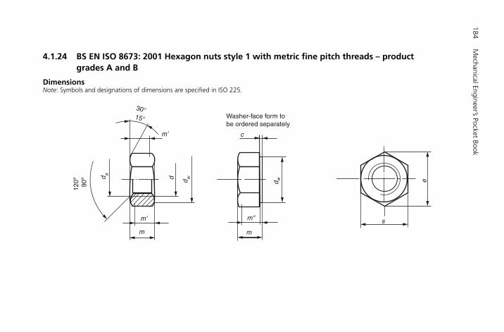
4.1.24 BS EN ISO 8673: 2001 Hexagon nuts style 1 with metric fine pitch threads – product grades A and B
DimensionsNote: Symbols and designations of dimensions are specified in ISO 225.
184M
echanical Engineer’s Pocket Book
120º
90º
30°d a
d wd
m
m'
m'
15°
m
m"
c
d w
Washer-face form tobe ordered separately
e
s
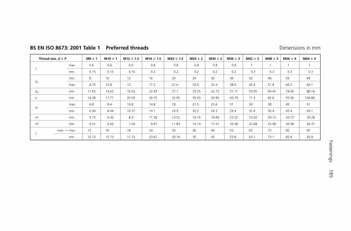
Fastenings185
Thread size, d � P M8 � 1 M10 � 1 M12 � 1.5 M16 � 1.5 M20 � 1.5 M24 � 2 M30 � 2 M36 � 3 M42 � 3 M48 � 3 M56 � 4 M64 � 4
cmax. 0.6 0.6 0.6 0.8 0.8 0.8 0.8 0.8 1 1 1 1
min. 0.15 0.15 0.15 0.2 0.2 0.2 0.2 0.2 0.3 0.3 0.3 0.3
da
min. 8 10 12 16 20 24 30 36 42 48 56 64
max. 8.75 10.8 13 17.3 21.6 25.9 32.4 38.9 45.4 51.8 60.5 69.1
dw min. 11.63 14.63 16.63 22.49 27.7 33.25 42.75 51.11 59.95 69.45 78.66 88.16
e min. 14.38 17.77 20.03 26.75 32.95 39.55 50.85 60.79 71.3 82.6 93.56 104.86
mmax. 6.8 8.4 10.8 14.8 18 21.5 25.6 31 34 38 45 51
min. 6.44 8.04 10.37 14.1 16.9 20.2 24.3 29.4 32.4 36.4 43.4 49.1
m� min. 5.15 6.43 8.3 11.28 13.52 16.16 19.44 23.52 25.92 29.12 34.72 39.28
m� min. 4.51 5.63 7.26 9.87 11.83 14.14 17.01 20.58 22.68 25.48 30.38 34.37
snom. � max. 13 16 18 24 30 36 46 55 65 75 85 95
min. 12.73 15.73 17.73 23.67 29.16 35 45 53.8 63.1 73.1 82.8 92.8
BS EN ISO 8673: 2001 Table 1 Preferred threads Dimensions in mm

186M
echanical Engineer’s Pocket Book
Thread size, d � P M10 � 1.25 M12 � 1.25 M14 � 1.5 M18 � 1.5 M20 � 2 M22 � 1.5 M27 � 2 M33 � 2 M39 � 3 M45 � 3 M52 � 4 M60 � 4
cmax. 0.6 0.6 0.6 0.8 0.8 0.8 0.8 0.8 1 1 1 1
min. 0.15 0.15 0.15 0.2 0.2 0.2 0.2 0.2 0.3 0.3 0.3 0.3
da
min. 10 12 14 18 20 22 27 33 39 45 52 60
max. 10.8 13 15.1 19.5 21.6 23.7 29.1 35.6 42.1 48.6 56.2 64.8
dw min. 14.63 16.63 19.64 24.85 27.7 31.35 38 46.55 55.86 64.7 74.2 83.41
e min. 17.77 20.03 23.36 29.56 32.95 37.29 45.2 55.37 66.44 76.95 88.25 99.21
mmax. 8.4 10.8 12.8 15.8 18 19.4 23.8 28.7 33.4 36 42 48
min. 8.04 10.37 12.1 15.1 16.9 18.1 22.5 27.4 31.8 34.4 40.4 46.4
m� min. 6.43 8.3 9.68 12.08 13.52 14.48 18 21.92 25.44 27.52 32.32 37.12
m� min. 5.63 7.26 8.47 10.57 11.83 12.67 15.75 19.18 22.26 24.08 28.28 32.48
snom. � max. 16 18 21 27 30 34 41 50 60 70 80 90
min. 15.73 17.73 20.67 26.16 29.16 33 40 49 58.8 68.1 78.1 87.8
BS EN ISO 8673: 2001 Table 2 Non-preferred threads Dimensions in mm
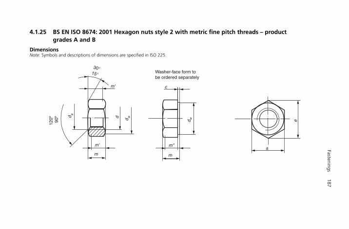
4.1.25 BS EN ISO 8674: 2001 Hexagon nuts style 2 with metric fine pitch threads – product grades A and B
DimensionsNote: Symbols and descriptions of dimensions are specified in ISO 225.
Fastenings187
120º
90º
30°d a
d wd
m
m'
m'
15°
m
m"
c
d w
Washer-face form tobe ordered separately
e
s
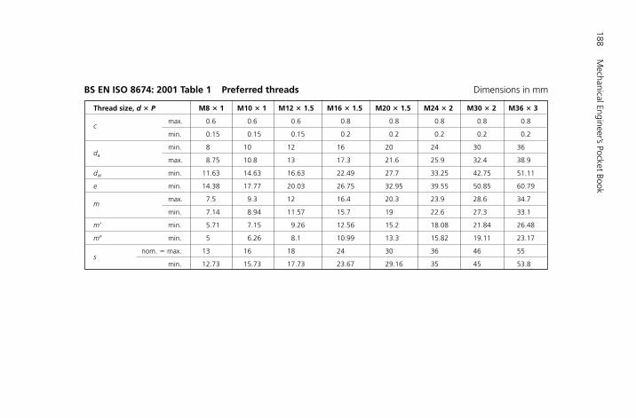
188M
echanical Engineer’s Pocket Book
Thread size, d � P M8 � 1 M10 � 1 M12 � 1.5 M16 � 1.5 M20 � 1.5 M24 � 2 M30 � 2 M36 � 3
cmax. 0.6 0.6 0.6 0.8 0.8 0.8 0.8 0.8
min. 0.15 0.15 0.15 0.2 0.2 0.2 0.2 0.2
da
min. 8 10 12 16 20 24 30 36
max. 8.75 10.8 13 17.3 21.6 25.9 32.4 38.9
dw min. 11.63 14.63 16.63 22.49 27.7 33.25 42.75 51.11
e min. 14.38 17.77 20.03 26.75 32.95 39.55 50.85 60.79
mmax. 7.5 9.3 12 16.4 20.3 23.9 28.6 34.7
min. 7.14 8.94 11.57 15.7 19 22.6 27.3 33.1
m� min. 5.71 7.15 9.26 12.56 15.2 18.08 21.84 26.48
m� min. 5 6.26 8.1 10.99 13.3 15.82 19.11 23.17
snom. � max. 13 16 18 24 30 36 46 55
min. 12.73 15.73 17.73 23.67 29.16 35 45 53.8
BS EN ISO 8674: 2001 Table 1 Preferred threads Dimensions in mm
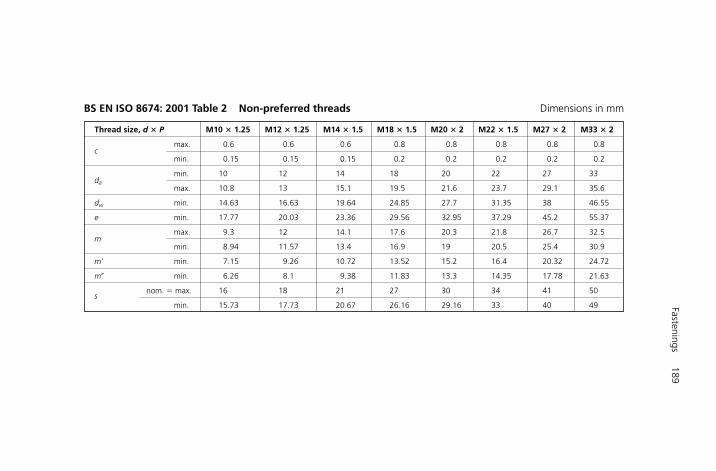
Fastenings189
Thread size, d � P M10 � 1.25 M12 � 1.25 M14 � 1.5 M18 � 1.5 M20 � 2 M22 � 1.5 M27 � 2 M33 � 2
cmax. 0.6 0.6 0.6 0.8 0.8 0.8 0.8 0.8
min. 0.15 0.15 0.15 0.2 0.2 0.2 0.2 0.2
da
min. 10 12 14 18 20 22 27 33
max. 10.8 13 15.1 19.5 21.6 23.7 29.1 35.6
dw min. 14.63 16.63 19.64 24.85 27.7 31.35 38 46.55
e min. 17.77 20.03 23.36 29.56 32.95 37.29 45.2 55.37
mmax. 9.3 12 14.1 17.6 20.3 21.8 26.7 32.5
min. 8.94 11.57 13.4 16.9 19 20.5 25.4 30.9
m� min. 7.15 9.26 10.72 13.52 15.2 16.4 20.32 24.72
m� min. 6.26 8.1 9.38 11.83 13.3 14.35 17.78 21.63
snom. � max. 16 18 21 27 30 34 41 50
min. 15.73 17.73 20.67 26.16 29.16 33 40 49
BS EN ISO 8674: 2001 Table 2 Non-preferred threads Dimensions in mm

4.1.26 BS EN ISO 8675: 2001 Hexagon thin nuts with metric fine pitch threads – product grades A and B
DimensionsNote: Symbols and descriptions of dimensions are specified in ISO 225.
190M
echanical Engineer’s Pocket Book
120º
90º
30°
d a d w
d
m
m'
m'
15°
e
s

Fastenings191
Thread size, d � P M8 � 1 M10 � 1 M12 � 1.5 M16 � 1.5 M20 � 1.5 M24 � 2 M30 � 2 M36 � 3 M42 � 3 M48 � 3 M56 � 4 M64 � 4
damin. 8 10 12 16 20 24 30 36 42 48 56 64
max. 8.75 10.8 13 17.3 21.6 25.9 32.4 38.9 45.4 51.8 60.5 69.1
dw min. 11.63 14.63 16.63 22.49 27.7 33.25 42.75 51.11 59.95 69.45 78.66 88.16
e min. 14.38 17.77 20.03 26.75 32.95 39.55 50.85 60.79 71.3 82.6 93.56 104.86
mmax. 4 5 6 8 10 12 15 18 21 24 28 32
min. 3.7 4.7 5.7 7.42 9.1 10.9 13.9 16.9 19.7 22.7 26.7 30.4
m� min. 2.96 3.76 4.56 5.94 7.28 8.72 11.12 13.52 15.76 18.16 21.36 24.32
snom.�max. 13 16 18 24 30 36 46 55 65 75 85 95
min. 12.73 15.73 17.73 23.67 29.16 35 45 53.8 63.1 73.1 82.8 92.8
BS EN ISO 8675: 2001 Table 1 Preferred threads Dimensions in mm
Thread size, d � P M10 � 1.25 M12 � 1.25 M14 � 1.5 M18 � 1.5 M20 � 2 M22 � 1.5 M27 � 2 M33 � 2 M39 � 3 M45 � 3 M52 � 4 M60 � 4
da
min. 10 12 14 18 20 22 27 33 39 45 52 60
max. 10.8 13 15.1 19.5 21.6 23.7 29.1 35.6 42.1 48.6 56.2 64.8
dw min. 14.63 16.63 19.64 24.85 27.7 31.35 38 46.55 55.86 64.7 74.2 83.41
e min. 17.77 20.03 23.36 29.56 32.95 37.29 45.2 55.37 66.44 76.95 88.25 99.21
mmax. 5 6 7 9 10 11 13.5 16.5 19.5 22.5 26 30
min. 4.7 5.7 6.42 8.42 9.1 9.9 12.4 15.4 18.2 21.2 24.7 28.7
m� min. 3.76 4.56 5.14 6.74 7.28 7.92 9.92 12.32 14.56 16.96 19.76 22.96
snom.�max. 16 18 21 27 30 34 41 50 60 70 80 90
min. 15.73 17.73 20.67 26.16 29.16 33 40 49 58.8 68.1 78.1 87.8
BS EN ISO 8675: 2001 Table 2 Non-preferred threads Dimensions in mm
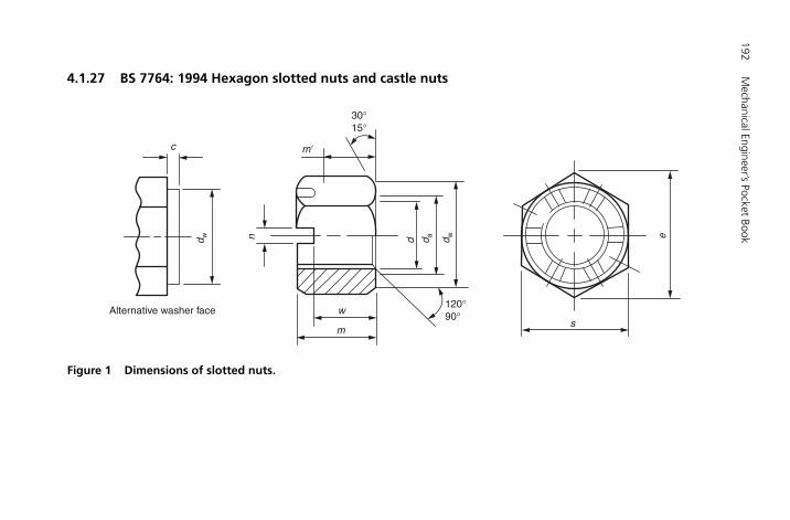
4.1.27 BS 7764: 1994 Hexagon slotted nuts and castle nuts
192M
echanical Engineer’s Pocket Book
Alternative washer face
c
w
ms
e
30°15°
120°90°
m�
u
d w d a d wd
Figure 1 Dimensions of slotted nuts.
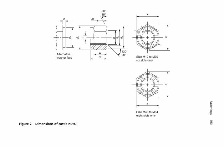
Fastenings193
Size M12 to M39six slots only
c
wm
e
Size M42 to M64eight slots only
e
s
s30°15°
120°Alternativewasher face
90°
m�
u
d w d e d a d wd
Figure 2 Dimensions of castle nuts.

194M
echanical Engineer’s Pocket Book
d M4 M5 M6 M8 M10 M12 (M14) M16 (M18) M20 (M22) M24 (M27) M30 (M33) M36 (M39) M42 (M45) M48 (M52) M56 (M60) M64
p 0.7 0.8 1 1.25 1.5 1.75 2 2 2.5 2.5 2.5 3 3 3.5 3.5 4 4 4.5 4.5 5 5 5.5 5.5 6
c max. 0.4 0.5 0.5 0.6 0.6 0.6 0.6 0.8 0.8 0.8 0.8 0.8 0.8 0.8 0.8 0.8 1 1 1 1 1 1 1 1
da
min. 4 5 6 8 10 12 14 16 18 20 22 24 27 30 33 36 39 42 45 48 52 56 60 64
max. 4.6 5.75 6.75 8.75 10.8 13 15.1 17.3 19.5 21.6 23.7 25.9 29.1 32.4 35.6 38.9 42.1 45.4 48.6 51.8 56.2 60.5 64.8 69.1
de
max. – – – – – 16 19 22 25 28 30 34 38 42 46 50 55 58 62 65 70 75 80 85
min. – – – – – 15.57 18.48 21.48 24.16 27.16 29.16 33 37 41 45 49 53.8 56.8 60.8 63.8 68.8 73.8 78.8 83.8
dw min. 5.9 6.9 8.9 11.6 14.6 16.6 19.6 22.5 24.8 27.7 31.4 33.2 38 42.7 46.6 51.1 55.9 59.9 64.7 69.4 74.2 78.7 83.4 88.2
e min. 7.66 8.79 11.05 14.38 17.77 20.03 23.36 26.75 29.58 32.95 37.29 39.55 45.2 50.85 55.37 60.79 66.44 71.3 76.95 82.6 88.25 93.56 99.21 104.86
mmax. 5 6 7.5 9.5 12 15 16 19 21 22 26 27 30 33 35 38 40 46 48 50 54 57 63 66
min. 4.7 5.7 7.14 9.14 11.57 14.57 15.57 18.48 21.48 21.48 25.48 25.48 29.48 32.38 34.38 37.38 39.38 45.38 47.38 49.38 53.26 56.26 62.26 65.26
m� min. 2.32 3.52 3.92 5.15 6.43 8.3 9.68 11.28 12.08 13.52 14.48 16.16 18 19.44 21.92 23.52 25.44 25.92 27.52 29.12 32.32 34.72 37.12 39.3
nmin. 1.2 1.4 2 2.5 2.8 3.5 3.5 4.5 4.5 4.5 5.5 5.5 5.5 7 7 7 7 9 9 9 9 9 11 11
max. 1.45 1.65 2.25 2.75 3.05 3.8 3.8 4.8 4.8 4.8 5.8 5.8 5.8 7.36 7.36 7.36 7.36 9.36 9.36 9.36 9.36 9.36 11.43 11.43
smax. 7 8 10 13 16 18 21 24 27 30 34 36 41 46 50 55 60 65 70 75 80 85 90 95
min. 6.78 7.78 9.78 12.73 15.73 17.73 20.67 23.67 26.16 29.16 33 35 40 45 49 53.8 58.8 63.1 68.1 73.1 78.1 82.8 87.8 92.8
wmax. 2.9 4 5 6.5 8 10 11 13 15 16 18 19 22 24 26 29 31 34 36 38 42 45 48 51
min. 3.2 3.7 4.7 6.14 7.64 9.64 10.57 12.59 14.57 15.57 17.57 18.48 21.48 23.48 25.48 28.48 30.38 33.38 35.38 37.38 41.38 44.38 47.38 50.26
For product grade A see Table 2 For product grade B see Table 2
BS 7764: 1994 Table 1 Dimensions of hexagon slotted nuts and castle nuts Dimensions in mm
Notes: 1. Non-preferred sizes are shown in brackets.2. Castle nuts shall not be specified below M12.3. Castle nuts above M39 shall have eight slots.

Fastenings195
Characteristic Requirement
Material Steel Stainless steel Non-ferrous metal
Thread tolerance Conforming to class 6H of BS 3643: Part 1: 1981 and BS 3643: Part 2: 1981
Mechanical propertiesa Conforming to material Conforming to material Conforming to BS EN 28839: 1992property class 6, 8 or 10 property class A2-70 of of BS EN 20898-2: 1992 BS 6105: 1981
Permissible dimensional Conforming to product grade A of BS 6322: Part 1: 1982 for thread sizes � M16deviations and deviations Conforming to product grade B of BS 6322: Part 1: 1982 for thread sizes � M16of form
Finish As processed with a As processed, unless As processed, unless otherwise lubricant, unless otherwise otherwise agreed between agreed between the purchaser agreed between the the purchaser and supplierc and supplierc
purchaser and supplierb,c
Acceptability In accordance with BS 6587: 1985
BS 7764: 1994 Table 2 Characteristics of hexagon slotted nuts and castle nuts
a Including the marking requirement.b The lubricant shall contain a rust inhibitor unless otherwise agreed between the purchaser and supplier.c Alternative surface finishes (e.g. electroplating) may be applied, if agreed between the purchaser and supplier.
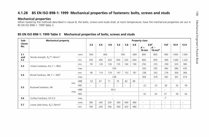
4.1.28 BS EN ISO 898-1: 1999 Mechanical properties of fasteners: bolts, screws and studs
Mechanical propertiesWhen tested by the methods described in clause 8, the bolts, screws and studs shall, at room temperature, have the mechanical properties set out inBS EN ISO 898-1: 1999 Table 3.
196M
echanical Engineer’s Pocket Book
Sub- Mechanical property Property classclause 3.6 4.6 4.8 5.6 5.8 6.8 8.8a 9.8c 10.9 12.9No. d � d �
16 mm 16 mmb
5.1 nom. 300 400 500 600 800 800 900 1 000 1 200and Tensile strength, Rm
d,e, N/mm2
5.2 min. 330 400 420 500 520 600 800 830 900 1 040 1 220
5.3 Vickers hardness, HV, F � 98 Nmin. 95 120 130 155 160 190 250 255 290 320 385
max. 250 320 335 360 380 435
5.4 Brinell hardness, HB, F � 30D2min. 90 114 124 147 152 181 238 242 276 304 366
max. 238 304 318 342 361 414
min.HRB 52 67 71 79 82 89 – – – – –
5.5 Rockwell hardness, HRHRC – – – – – – 22 23 28 32 39
max.HRB 99.5 – – – – –
HRC – 32 34 37 39 44
5.6 Surface hardness, HV 0.3 max. – –f
5.7 Lower yield stress, ReLg, N/mm2
nom. 180 240 320 300 400 480 – – – – –
min. 190 240 340 300 420 480 – – – – –
BS EN ISO 898-1: 1999 Table 3 Mechanical properties of bolts, screws and studs

Fastenings197
a For bolts of property class 8.8 in diameters d � 16 mm, there is an increased risk of nut stripping in the case of inadvertent over-tightening inducting a load in excess of proofing load. Reference to ISO 898.2 is recommended.
b For structural bolting the limit is 12 mm.c Applies only to nominal thread diameters d � 16 mm.d Minimum tensile properties apply to products of nominal length l � 2.5d. Minimum hardness applies to products of length l � 2.5d and other products which cannot
be tensile tested (e.g. due to head configuration).e For testing of full-size bolts, screws and studs, the loads given in BS EN ISO 898-1: 1999 Tables 6 to 9 (of the full standard) shall be applied.f Surface hardness shall not be more than 30 Vickers points above the measured core hardness on the product when readings of both surface and core are carried out atHV 0.3. For property class 10.9, any increase in hardness at the surface which indicates that the surface hardness exceeds 390 HV is not acceptable.
g In cases where the lower yield stress ReL cannot be determined, it is permissible to measure the proof stress Rp0.2.
5.8 Proof stress, Rp0.2, N/mm2nom. – 640 640 720 900 1080
min. – 640 660 720 940 1100
5.9 Stress under proofing load, Sp
Sp/ReL or Sp/Rp0.2 0.94 0.94 0.91 0.93 0.90 0.92 0.91 0.91 0.90 0.88 0.88
N/mm2 180 225 310 280 380 440 580 600 650 830 970
5.10 Elongation after fracture, A min. 25 22 14 20 10 8 12 12 10 9 8
5.11 Strength under wedge loadinge The values for full size bolts and screws (not studs) shall not be smaller than the minimum values for tensile strength shown in 5.2
5.12 Impact strength, J min. – 25 – 30 30 25 20 15
5.13 Head soundness no fracture
5.14
Minimum height of non-decarburized –
1 H12
H13
H1thread zone, E 2 3 4
Maximum depth of complete mm – 0.015decarburization, G

Mechanical properties to be determinedTwo test programmes, A and B, for mechanical properties of bolts, screws and studs, using the methods described in clause 8, are set out in BS EN ISO898-1: 1999 Table 5.
The application of programme B is always desirable, but is mandatory for products with breaking loads less than 500 kN. Programme A is suitable formachined test pieces and for bolts with a shank area less than the stress area.
198M
echanical Engineer’s Pocket Book
Size Bolts and screws with thread Bolts and screws with thread diameter d � 4 mm diameter d � 4 mm or length l � 2.5da and length l � 2.5d
Test decisive for acceptance � �
a Also bolts and screws with special head or shank configurations which are weaker than the threaded section.
BS EN ISO 898-1: 1999 Table 4 Key to test programmes (see BS EN ISO898-1: 1999 Table 5)
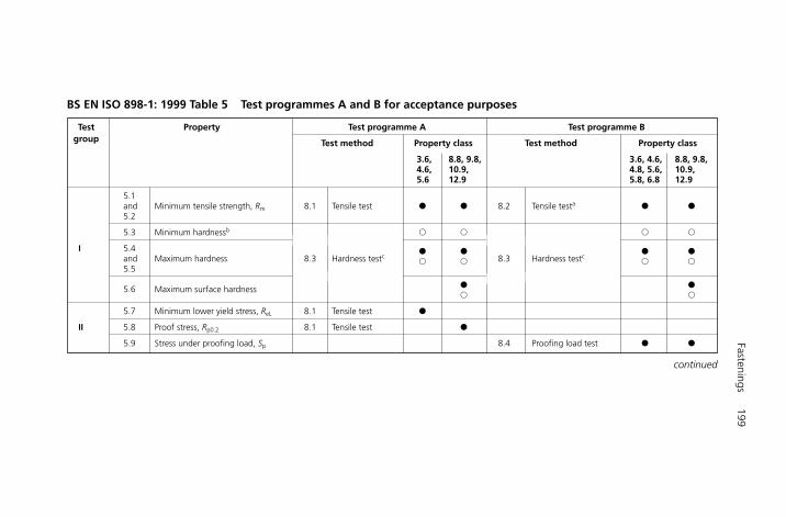
Fastenings199
Test Property Test programme A Test programme Bgroup Test method Property class Test method Property class
3.6, 8.8, 9.8, 3.6, 4.6, 8.8, 9.8, 4.6, 10.9, 4.8, 5.6, 10.9,5.6 12.9 5.8, 6.8 12.9
5.1and Minimum tensile strength, Rm 8.1 Tensile test � � 8.2 Tensile testa � �
5.2
5.3 Minimum hardnessb � � � �
I 5.4 � � � �and Maximum hardness 8.3 Hardness testc 8.3 Hardness testc
5.5� � � �
5.6 Maximum surface hardness � �
� �
5.7 Minimum lower yield stress, ReL 8.1 Tensile test �
II 5.8 Proof stress, Rp0.2 8.1 Tensile test �
5.9 Stress under proofing load, Sp 8.4 Proofing load test � �
BS EN ISO 898-1: 1999 Table 5 Test programmes A and B for acceptance purposes
continued
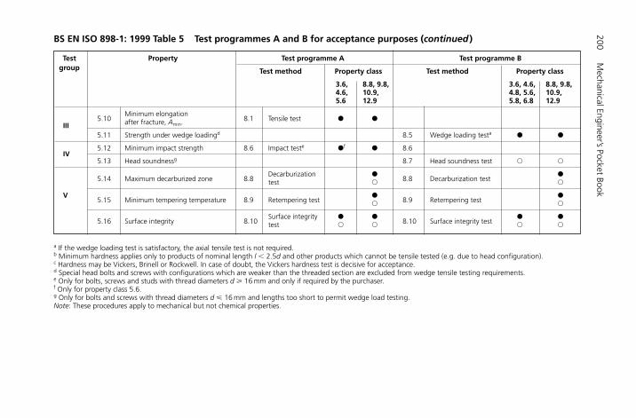
200M
echanical Engineer’s Pocket Book
Test Property Test programme A Test programme Bgroup Test method Property class Test method Property class
3.6, 8.8, 9.8, 3.6, 4.6, 8.8, 9.8, 4.6, 10.9, 4.8, 5.6, 10.9,5.6 12.9 5.8, 6.8 12.9
5.10Minimum elongation
8.1 Tensile test � �after fracture, Amin.III5.11 Strength under wedge loadingd 8.5 Wedge loading testa � �
IV5.12 Minimum impact strength 8.6 Impact teste �f � 8.6
5.13 Head soundnessg 8.7 Head soundness test � �
5.14 Maximum decarburized zone 8.8Decarburization �
8.8 Decarburization test�
test � �
V5.15 Minimum tempering temperature 8.9 Retempering test
�8.9 Retempering test
�
� �
5.16 Surface integrity 8.10Surface integrity � �
8.10 Surface integrity test� �
test � � � �
a If the wedge loading test is satisfactory, the axial tensile test is not required.b Minimum hardness applies only to products of nominal length l � 2.5d and other products which cannot be tensile tested (e.g. due to head configuration).c Hardness may be Vickers, Brinell or Rockwell. In case of doubt, the Vickers hardness test is decisive for acceptance.d Special head bolts and screws with configurations which are weaker than the threaded section are excluded from wedge tensile testing requirements.e Only for bolts, screws and studs with thread diameters d 16 mm and only if required by the purchaser.f Only for property class 5.6.g Only for bolts and screws with thread diameters d � 16 mm and lengths too short to permit wedge load testing.Note: These procedures apply to mechanical but not chemical properties.
BS EN ISO 898-1: 1999 Table 5 Test programmes A and B for acceptance purposes (continued )
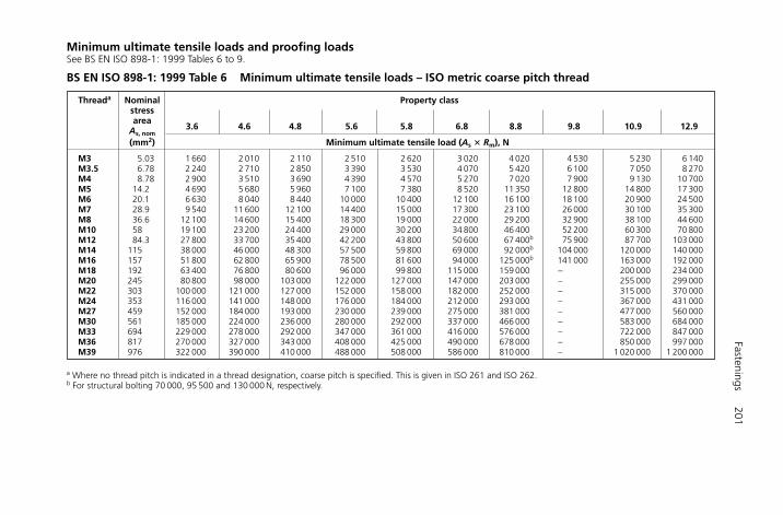
Minimum ultimate tensile loads and proofing loadsSee BS EN ISO 898-1: 1999 Tables 6 to 9.
BS EN ISO 898-1: 1999 Table 6 Minimum ultimate tensile loads – ISO metric coarse pitch thread
Fastenings201
Nominal Property classThreada
stress area
As, nom3.6 4.6 4.8 5.6 5.8 6.8 8.8 9.8 10.9 12.9
(mm2) Minimum ultimate tensile load (As � Rm), N
M3 5.03 1 660 2 010 2 110 2 510 2 620 3 020 4 020 4 530 5 230 6 140M3.5 6.78 2 240 2 710 2 850 3 390 3 530 4 070 5 420 6 100 7 050 8 270M4 8.78 2 900 3 510 3 690 4 390 4 570 5 270 7 020 7 900 9 130 10 700M5 14.2 4 690 5 680 5 960 7 100 7 380 8 520 11 350 12 800 14 800 17 300M6 20.1 6 630 8 040 8 440 10 000 10 400 12 100 16 100 18 100 20 900 24 500M7 28.9 9 540 11 600 12 100 14 400 15 000 17 300 23 100 26 000 30 100 35 300M8 36.6 12 100 14 600 15 400 18 300 19 000 22 000 29 200 32 900 38 100 44 600M10 58 19 100 23 200 24 400 29 000 30 200 34 800 46 400 52 200 60 300 70 800M12 84.3 27 800 33 700 35 400 42 200 43 800 50 600 67 400b 75 900 87 700 103 000M14 115 38 000 46 000 48 300 57 500 59 800 69 000 92 000b 104 000 120 000 140 000M16 157 51 800 62 800 65 900 78 500 81 600 94 000 125 000b 141 000 163 000 192 000M18 192 63 400 76 800 80 600 96 000 99 800 115 000 159 000 – 200 000 234 000M20 245 80 800 98 000 103 000 122 000 127 000 147 000 203 000 – 255 000 299 000M22 303 100 000 121 000 127 000 152 000 158 000 182 000 252 000 – 315 000 370 000M24 353 116 000 141 000 148 000 176 000 184 000 212 000 293 000 – 367 000 431 000M27 459 152 000 184 000 193 000 230 000 239 000 275 000 381 000 – 477 000 560 000M30 561 185 000 224 000 236 000 280 000 292 000 337 000 466 000 – 583 000 684 000M33 694 229 000 278 000 292 000 347 000 361 000 416 000 576 000 – 722 000 847 000M36 817 270 000 327 000 343 000 408 000 425 000 490 000 678 000 – 850 000 997 000M39 976 322 000 390 000 410 000 488 000 508 000 586 000 810 000 – 1 020 000 1 200 000
a Where no thread pitch is indicated in a thread designation, coarse pitch is specified. This is given in ISO 261 and ISO 262.b For structural bolting 70 000, 95 500 and 130 000 N, respectively.

202M
echanical Engineer’s Pocket Book
Nominal Property classThreada
stress area
As,nom3.6 4.6 4.8 5.6 5.8 6.8 8.8 9.8 10.9 12.9
(mm2) Proofing load (As � Sp), N
M3 5.03 910 1 130 1 560 1 410 1 910 2 210 2 920 3 270 4 180 4 880M3.5 6.78 1 220 1 530 2 100 1 900 2 580 2 980 3 940 4 410 5 630 6 580M4 8.78 1 580 1 980 2 720 2 460 3 340 3 860 5 100 5 710 7 290 8 520M5 14.2 2 560 3 200 4 400 3 980 5 400 6 250 8 230 9 230 11 800 13 800M6 20.1 3 620 4 520 6 230 5 630 7 640 8 840 11 600 13 100 16 700 19 500M7 28.9 5 200 6 500 8 960 8 090 11 000 12 700 16 800 18 800 24 000 28 000M8 36.6 6 590 8 240 11 400 10 200 13 900 16 100 21 200 23 800 30 400 35 500M10 58 10 400 13 000 18 000 16 200 22 000 25 500 33 700 37 700 48 100 56 300M12 84.3 15 200 19 000 26 100 23 600 32 000 37 100 48 900b 54 800 70 000 81 800M14 115 20 700 25 900 35 600 32 200 43 700 50 600 66 700b 74 800 95 500 112 000M16 157 28 300 35 300 48 700 44 000 59 700 69 100 91 000b 102 000 130 000 152 000M18 192 34 600 43 200 59 500 53 800 73 000 84 500 115 000 – 159 000 186 000M20 245 44 100 55 100 76 000 68 600 93 100 108 000 147 000 – 203 000 238 000M22 303 54 500 68 200 93 900 84 800 115 000 133 000 182 000 – 252 000 294 000M24 353 63 500 79 400 109 000 98 800 134 000 155 000 212 000 – 293 000 342 000M27 459 82 600 103 000 142 000 128 000 174 000 202 000 275 000 – 381 000 445 000M30 561 101 000 126 000 174 000 157 000 213 000 247 000 337 000 – 466 000 544 000M33 694 125 000 156 000 215 000 194 000 264 000 305 000 416 000 – 570 000 673 000M36 817 147 000 184 000 253 000 229 000 310 000 359 000 490 000 – 678 000 792 000M39 976 176 000 220 000 303 000 273 000 371 000 429 000 586 000 – 810 000 947 000
BS EN ISO 898-1: 1999 Table 7 Proofing loads ISO metric coarse pitch thread
a Where no thread pitch is indicated in a thread designation, coarse pitch is specified. This is given in ISO 261 and ISO 262.b For structural bolting 50 700, 68 800 and 94 500 N, respectively.
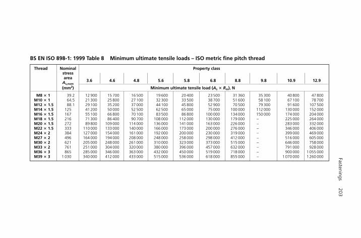
Fastenings203
Nominal Property classThreadstress area
As,nom3.6 4.6 4.8 5.6 5.8 6.8 8.8 9.8 10.9 12.9
(mm2) Minimum ultimate tensile load (As � Rm), N
M8 � 1 39.2 12 900 15 700 16 500 19 600 20 400 23 500 31 360 35 300 40 800 47 800M10 � 1 64.5 21 300 25 800 27 100 32 300 33 500 38 700 51 600 58 100 67 100 78 700M12 � 1.5 88.1 29 100 35 200 37 000 44 100 45 800 52 900 70 500 79 300 91 600 107 500M14 � 1.5 125 41 200 50 000 52 500 62 500 65 000 75 000 100 000 112 000 130 000 152 000M16 � 1.5 167 55 100 66 800 70 100 83 500 86 800 100 000 134 000 150 000 174 000 204 000M18 � 1.5 216 71 300 86 400 90 700 108 000 112 000 130 000 179 000 – 225 000 264 000M20 � 1.5 272 89 800 109 000 114 000 136 000 141 000 163 000 226 000 – 283 000 332 000M22 � 1.5 333 110 000 133 000 140 000 166 000 173 000 200 000 276 000 – 346 000 406 000M24 � 2 384 127 000 154 000 161 000 192 000 200 000 230 000 319 000 – 399 000 469 000M27 � 2 496 164 000 194 000 208 000 248 000 258 000 298 000 412 000 – 516 000 605 000M30 � 2 621 205 000 248 000 261 000 310 000 323 000 373 000 515 000 – 646 000 758 000M33 � 2 761 251 000 304 000 320 000 380 000 396 000 457 000 632 000 – 791 000 928 000M36 � 3 865 285 000 346 000 363 000 432 000 450 000 519 000 718 000 – 900 000 1 055 000M39 � 3 1 030 340 000 412 000 433 000 515 000 536 000 618 000 855 000 – 1 070 000 1 260 000
BS EN ISO 898-1: 1999 Table 8 Minimum ultimate tensile loads – ISO metric fine pitch thread
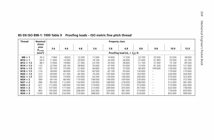
204M
echanical Engineer’s Pocket Book
Nominal Property classThreadstress area
As,nom3.6 4.6 4.8 5.6 5.8 6.8 8.8 9.8 10.9 12.9
(mm2) Proofing load (As � Sp), N
M8 � 1 39.2 7 060 8 820 12 200 11 000 14 900 17 200 22 700 25 500 32 500 38 000M10 � 1 64.5 11 600 14 500 20 000 18 100 24 500 28 400 37 400 41 900 53 500 62 700M12 � 1.5 88.1 15 900 19 800 27 300 24 700 33 500 38 800 51 100 57 300 73 100 85 500M14 � 1.5 125 22 500 28 100 38 800 35 000 47 500 55 000 72 500 81 200 104 000 121 000M16 � 1.5 167 30 100 37 600 51 800 46 800 63 500 73 500 96 900 109 000 139 000 162 000M18 � 1.5 216 38 900 48 600 67 000 60 500 82 100 95 000 130 000 – 179 000 210 000M20 � 1.5 272 49 000 61 200 84 300 76 200 103 000 120 000 163 000 – 226 000 264 000M22 � 1.5 333 59 900 74 900 103 000 93 200 126 000 146 000 200 000 – 276 000 323 000M24 � 2 384 69 100 86 400 119 000 108 000 146 000 169 000 230 000 – 319 000 372 000M27 � 2 496 89 300 112 000 154 000 139 000 188 000 218 000 298 000 – 412 000 481 000M30 � 2 621 112 000 140 000 192 000 174 000 236 000 273 000 373 000 – 515 000 602 000M33 � 2 761 137 000 171 000 236 000 213 000 289 000 335 000 457 000 – 632 000 738 000M36 � 3 865 156 000 195 000 268 000 242 000 329 000 381 000 519 000 – 718 000 839 000M39 � 3 1 030 185 000 232 000 319 000 288 000 391 000 453 000 618 000 – 855 000 999 000
BS EN ISO 898-1: 1999 Table 9 Proofing loads – ISO metric fine pitch thread

Fastenings 205
4.1.29 BS EN ISO 898-1: 1999 Marking
SymbolsMarking symbols are shown in BS EN ISO 898-1: 1999 Table 1.
Identification
Hexagon bolts and screwsHexagon bolts and screws shall be marked with the designation symbol of the propertyclass described in clause 3.
The marking is obligatory for all property classes, preferably on the top of the head byindenting or embossing or on the side of the head by indenting (see Fig. 1).
Marking is required for hexagon bolts and screws with nominal diameters d � 5 mmwhere the shape of the product allows it, preferably on the head.
Hexagon socket head cap screwsHexagon socket head cap screws shall be marked with the designation symbol of theproperty class described in clause 3.
The marking is obligatory for property classes equal to or higher than 8.8, preferably onthe side of the head by indenting or on the top of the head by indenting or embossing(see Fig. 2).
Marking is required for hexagon socket head cap screws with nominal diametersd � 5 mm where the shape of the product allows it, preferably on the head.
The clock-face marking system as given for nuts in ISO 898-2 may be used as an alterna-tive method on small hexagon socket head cap screws.
H6508-Ch04.1d.qxd 9/21/05 3:12 PM Page 205

206M
echanical Engineer’s Pocket Book
12.9
12.9
8.8
8.8
Figure 1 Examples of marking on hexagon bolts andscrews.
Figure 2 Examples of marking on hexagon sockethead cap screws.
Property class 3.6 4.6 4.8 5.6 5.8 6.8 8.8 9.8 10.9 12.9
Marking symbola,b 3.6 4.6 4.8 5.6 5.8 6.8 8.8 9.8 10.9 12.9
BS EN ISO 898-1: 1999 Table 1 Marking symbols
aThe full-stop in the marking symbol may be omitted.bWhen low carbon martensitic steels are used for property class 10.9 (see BS EN ISO 898-1: 1999 Table 2), the symbol 10.9 shall be underlined: 10.9.

StudsStuds shall be marked with the designation symbol of the property class described in clause 3.
The marking is obligatory for property classes equal to or higher than 8.8, preferably onthe extreme end of the threaded portion by indenting (see Fig. 3). For studs with inter-ference fit, the marking shall be at the nut end.
Marking is required for studs with nominal diameters equal to or greater than 5 mm.
The symbols in BS EN ISO 898-1: 1999 Table 2 are permissible as an alternative identifi-cation method.
Other types of bolts and screwsThe same marking system as described in the sections Hexagon bolts and screws, andHexagon socket head cap screws shall be used for other types of bolts and screws ofproperty classes 4.6, 5.6 and all classes equal to or higher than 8.8, as described in theappropriate International Standards or, for special components, as agreed between theinterested parties.
Fastenings 207
Property class 8.8 9.8 10.9 12.9
Identification mark � � � �
BS EN ISO 898-1: 1999 Table 2 Identification marksfor studs
8.8
Figure 3 Marking of stud.
H6508-Ch04.1d.qxd 9/21/05 3:12 PM Page 207
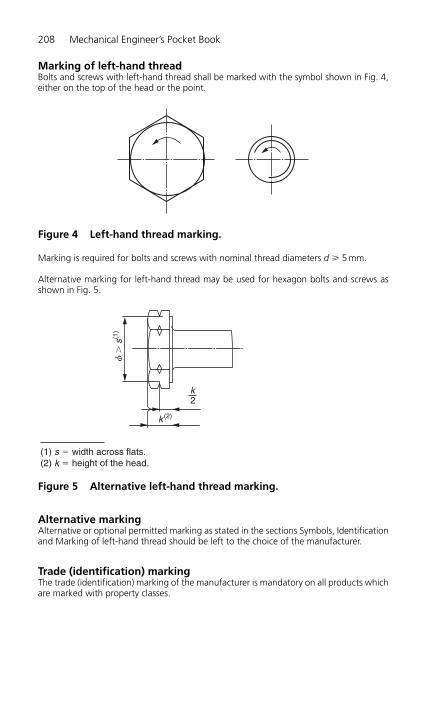
Marking of left-hand threadBolts and screws with left-hand thread shall be marked with the symbol shown in Fig. 4,either on the top of the head or the point.
Marking is required for bolts and screws with nominal thread diameters d � 5 mm.
Alternative marking for left-hand thread may be used for hexagon bolts and screws asshown in Fig. 5.
Alternative markingAlternative or optional permitted marking as stated in the sections Symbols, Identificationand Marking of left-hand thread should be left to the choice of the manufacturer.
Trade (identification) markingThe trade (identification) marking of the manufacturer is mandatory on all products whichare marked with property classes.
208 Mechanical Engineer’s Pocket Book
Figure 4 Left-hand thread marking.
f�
s(1)
k
k (2)
2
(1) s � width across flats.(2) k � height of the head.
Figure 5 Alternative left-hand thread marking.
H6508-Ch04.1d.qxd 9/21/05 3:12 PM Page 208
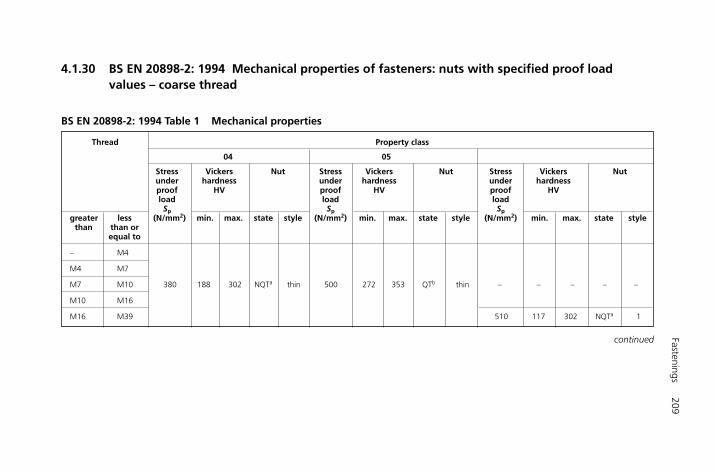
Fastenings209
Thread Property class
04 05
Stress Vickers Nut Stress Vickers Nut Stress Vickers Nutunder hardness under hardness under hardnessproof HV proof HV proof HVload load loadSp Sp Sp
greater less (N/mm2) min. max. state style (N/mm2) min. max. state style (N/mm2) min. max. state stylethan than or
equal to
– M4
M4 M7
M7 M10 380 188 302 NQTa thin 500 272 353 QTb thin – – – – –
M10 M16
M16 M39 510 117 302 NQTa 1
BS EN 20898-2: 1994 Table 1 Mechanical properties
4.1.30 BS EN 20898-2: 1994 Mechanical properties of fasteners: nuts with specified proof load values – coarse thread
continued
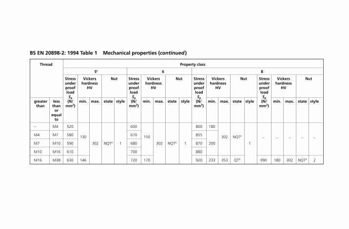
Thread Property class
5c 6 8
Stress Vickers Nut Stress Vickers Nut Stress Vickers Nut Stress Vickers Nutunder hardness under hardness under hardness under hardnessproof HV proof HV proof HV proof HVload load load loadSp Sp Sp Sp
greater less (N/ min. max. state style (N/ min. max. state style (N/ min. max. state style (N/ min. max. state stylethan than mm2) mm2) mm2) mm2)
or equal
to
– M4 520 600 800 180
M4 M7 580 130 670 150 855 302 NQTa – – – – –
M7 M10 590 302 NQTa 1 680 302 NQTa 1 870 200 1
M10 M16 610 700 880
M16 M38 630 146 720 170 920 233 353 QTb 990 180 302 NQTa 2
BS EN 20898-2: 1994 Table 1 Mechanical properties (continued )
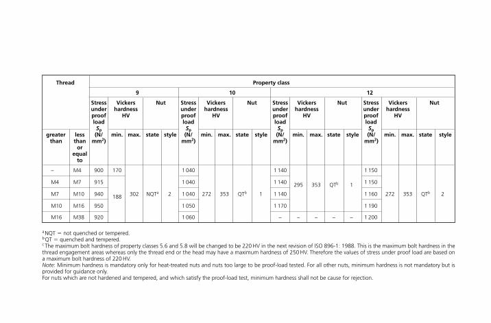
Thread Property class
9 10 12
Stress Vickers Nut Stress Vickers Nut Stress Vickers Nut Stress Vickers Nutunder hardness under hardness under hardness under hardnessproof HV proof HV proof HV proof HVload load load loadSp Sp Sp Sp
greater less (N/ min. max. state style (N/ min. max. state style (N/ min. max. state style (N/ min. max. state stylethan than mm2) mm2) mm2) mm2)
or equal
to
– M4 900 170 1 040 1 140 1 150
M4 M7 915 1 040 1 140 295 353 QTb 1 1 150
M7 M10 940 188 302 NQTa 2 1 040 272 353 QTb 1 1 140 1 160 272 353 QTb 2
M10 M16 950 1 050 1 170 1 190
M16 M38 920 1 060 – – – – – 1 200
aNQT � not quenched or tempered.bQT � quenched and tempered.c The maximum bolt hardness of property classes 5.6 and 5.8 will be changed to be 220 HV in the next revision of ISO 896-1: 1988. This is the maximum bolt hardness in thethread engagement areas whereas only the thread end or the head may have a maximum hardness of 250 HV. Therefore the values of stress under proof load are based ona maximum bolt hardness of 220 HV.Note: Minimum hardness is mandatory only for heat-treated nuts and nuts too large to be proof-load tested. For all other nuts, minimum hardness is not mandatory but isprovided for guidance only.For nuts which are not hardened and tempered, and which satisfy the proof-load test, minimum hardness shall not be cause for rejection.

Proof load valuesProof load values are given in BS EN 20898-2: 1994 Table 2.The nominal stress area As is calculated as follows:
where:
d2 � basic pitch diameter of the external thread (see ISO 724);d3 � minor diameter of the external thread;
where:
d1 � basic minor diameter of the external thread;H � height of the fundamental triangle of the thread.
d dH
3 1� �6
Ad d
s2 3
4 2�
� �⎛
⎝⎜⎜⎜⎜⎜
⎞
⎠
⎟⎟⎟⎟⎟
2
212 Mechanical Engineer’s Pocket Book
H6508-Ch04.1d.qxd 9/21/05 3:12 PM Page 212
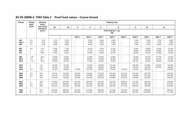
Thread Thread Nominal Property classpitch stress
04 05 4 5 6 8 9 10 12(mm) area of themandrel As
Proof load (As � Sp)(mm2)(N)
style 1 style 1 style 1 style 1 style 2 style 2 style 1 style 1 style 2
M3 0.5 5.03 1 910 2 500 – 2 600 3 000 4 000 – 4 500 5 200 5 700 5 800M3.5 0.6 6.78 2 580 3 400 – 3 550 4 050 5 400 – 6 100 7 050 7 700 7 800M4 0.7 8.78 3 340 4 400 – 4 550 5 250 7 000 – 7 900 9 150 10 000 10 100
M5 0.8 14.2 5 400 7 100 – 8 250 9 500 12 140 – 13 000 14 800 16 200 16 300M6 1 20.1 7 640 10 000 – 11 700 13 500 17 200 – 18 400 20 900 22 900 23 100M7 1 28.9 11 000 14 500 – 16 800 19 400 24 700 – 26 400 30 100 32 900 33 200
M8 1.25 36.6 13 900 18 300 – 21 600 24 900 31 800 – 34 400 38 100 41 700 42 500M10 1.5 58 22 000 29 000 – 34 200 39 400 50 500 – 54 500 60 300 66 100 67 300M12 1.75 84.3 32 000 42 200 – 51 400 59 000 74 200 – 80 100 88 500 98 600 100 300
M14 2 115 43 700 57 500 – 70 200 80 500 101 200 – 109 300 120 800 134 600 136 900M16 2 157 59 700 78 500 – 95 800 109 900 138 200 – 149 200 164 900 183 700 186 800M18 2.5 192 73 000 96 000 97 900 121 000 138 200 176 600 170 900 176 600 203 500 – 230 400
M20 2.5 245 93 100 122 500 125 000 154 400 176 400 225 400 218 100 225 400 259 700 – 294 000M22 2.5 303 115 100 151 500 154 500 190 900 218 200 278 800 269 700 278 800 321 200 – 363 600M24 3 353 134 100 176 500 180 000 222 400 254 200 324 800 314 200 324 800 374 200 – 423 600
M27 3 459 174 400 229 500 234 100 289 200 330 500 422 300 408 500 422 300 486 500 – 550 800M30 3.5 561 213 200 280 500 286 100 353 400 403 900 516 100 499 300 516 100 594 700 – 673 200M33 3.5 694 263 700 347 000 353 900 437 200 499 700 638 500 617 700 638 500 735 600 – 832 800
M36 4 817 310 500 408 500 416 700 514 700 588 200 751 600 727 100 751 600 866 000 – 980 400M39 4 976 370 900 488 000 497 800 614 900 702 700 897 900 868 600 897 900 1 035 000 – 1 171 000
BS EN 20898-2: 1994 Table 2 Proof load values – Coarse thread
Property class
either designationsymbol
aThe marking dot cannot be replaced by the manufacturer’s mark.
or code symbol(clock-face system)
Alt
ern
ativ
e m
arki
ng
4
4
5
5
6
6
8
8
9
9
10 12a
10 12
BS EN 20898-2: 1994 Table 3 Marking symbols for nuts with property classes in accordance with BS EN 20898-2 clause 3.1
BS EN 20898-2: 1994 Table 4 Marking symbols for nuts with propertyclasses in accordance with BS EN 20898-2 clause 3.2
Property class
Marking
04 05
04 05

Marking of left-hand threadNuts with left-hand thread shall be marked as shown in Fig. 1 on one bearing surface ofthe nut by indenting.
Fastenings 215
Figure 1 Left-hand thread marking.
f�
s(1)
(1) s � width across flats.
Figure 2 Alternative left-hand thread marking.
Marking is required for nuts with threads �M5.
The alternative marking for left-hand thread shown in Fig. 2 may also be used.
H6508-Ch04.1d.qxd 9/21/05 3:12 PM Page 215

216 Mechanical Engineer’s Pocket Book
Alternative markingAlternative or optional permitted marking as stated in the sections Symbols, Identifica-tion and Marking of left-hand thread under Section 4.1.29 is left to the choice of themanufacturer.
Trade (identification) markingThe trade (identification) marking of the manufacturer is mandatory on all products covered by the obligatory marking requirements for property classes, provided this is possible for technical reasons. Packages, however, shall be marked in all cases.
H6508-Ch04.1d.qxd 9/21/05 3:12 PM Page 216

Fastenings217
4.1.31 BS EN ISO 898-6: 1996 Mechanical properties of fasteners:nuts with specified proof load values – fine pitch thread
Property class of nut Mating bolts Nuts
Style 1 Style 2
Property class Nominal thread Nominal thread diameter range diameter range (mm)
(mm)
53.6, 4.6, 4.8
d � 39 d � 39 –5.6, 5.8
6 6.8 d � 39 d � 39 –
8 8.8 d � 39 d � 39 d � 16
10 10.9 d � 39 d � 16 d � 39
12 12.9 d � 16 – d � 16
BS EN ISO 898-6: 1996 Table 1 Designation system for nuts with nominalheights �0.8d
Note: In general, nuts of a higher property class can replace nuts of a lower property class. This is advisable for abolt/nut assembly going into a stress higher than the yield stress or the stress under proof load of the bolt.
218 Mechanical Engineer’s Pocket Book
However, should tightening beyond bolt proof load take place, the net design is intendedto ensure at least 10% of the over-tightened assemblies fail through bolt breakage inorder to warn the user that the installation practice is not appropriate.
Note: For more detailed information on the strength of screw thread assemblies and forthe styles of nuts, see ISO 898-2: 1992, Annex A.
Nuts with nominal heights �0.5d and �0.8d (effective heights ofthread �0.4d and �0.6d)Nuts with nominal heights �0.5d and �0.8d (effective height of thread �0.4d and �0.6d)are designated by a combination of two numbers: the second indicates the nominal stressunder proof load on a hardened test mandrel, while the first indicates that the load abilityof a bolt-nut assembly is reduced in comparison with the loadability on a hardened testmandrel and also in comparison with a bolt-nut assembly described in Section 3.1. Theeffective loading capacity is not only determined by the hardness of the nut and the effec-tive height of thread but also by the tensile strength of the bolt with which the nut is assem-bled. BS EN ISO 898-6: 1996 Table 2 gives the designation system and the stresses underproof load of the nuts. Proof loads are shown in BS EN ISO 898-6: 1996 Table 3. A guide forminimum expected stripping strengths of the joints when these nuts are assembled withbolts of various property classes is shown in BS EN ISO 898-6: 1996 Table 4.
Property class Nominal stress Actual stress of nut under proof under proof
load load (N/mm2) (N/mm2)
04 400 380
05 500 500
BS EN ISO 898-6: 1996 Table 2 Designation systemand stresses under proof load for nuts with nominalheights �0.5d and �0.8d
H6508-Ch04.1d.qxd 9/21/05 3:12 PM Page 218
Fastenings219
Thread Nominal Property classsize, stress area 04 05 5 6 8 10 12
d � P of mandrelProof load (As � Sp)As
(N)(mm2)
style 1 style 1 style 1 style 2 style 1 style 2 style 2
M8 �1 39.2 14 900 19 600 27 000 30 200 37 400 34 900 43 100 41 400 47 000M10 �1 64.5 24 500 32 200 44 500 49 700 61 600 57 400 71 000 68 000 77 400M10 �1.25 61.2 23 300 30 600 44 200 47 100 58 400 54 500 67 300 64 600 73 400
M12 �1.25 92.1 35 000 46 000 63 500 71 800 88 000 82 000 102 200 97 200 110 500M12 �1.5 88.1 33 500 44 000 60 800 68 700 84 100 78 400 97 800 92 900 105 700M14 �1.5 125 47 500 62 500 86 300 97 500 119 400 111 200 138 800 131 900 150 000
M16 �1.5 167 63 500 83 500 115 200 130 300 159 500 148 600 185 400 176 200 200 400M18 �1.5 215 81 700 107 500 154 800 187 000 221 500 – – 232 200 –M18 �2 204 77 500 102 000 146 900 177 500 210 100 – – 220 300 –
M20 �1.5 272 103 400 136 000 195 800 236 600 280 200 – – 293 800 –M20 � 2 258 98 000 129 000 185 800 224 500 265 700 – – 278 600 –M22 � 1.5 333 126 500 166 500 239 800 289 700 343 000 – – 359 600 –
M22 � 2 318 120 800 159 000 229 000 276 700 327 500 – – 343 400 –M24 � 2 384 145 900 192 000 276 500 334 100 395 500 – – 414 700 –M27 � 2 496 188 500 248 000 351 100 431 500 510 900 – – 535 700 –
M30 � 2 621 236 000 310 500 447 100 540 300 639 600 – – 670 700 –M33 � 2 761 289 200 380 500 547 900 662 100 783 800 – – 821 900 –M36 � 3 865 328 700 432 500 622 800 804 400 942 800 – – 934 200 –
M39 � 3 1 030 391 400 515 000 741 600 957 900 1 123 000 – – 1 112 000 –
BS EN ISO 898-6: 1996 Table 3 Proof load values
220 Mechanical Engineer’s Pocket Book
MaterialsNuts of property classes 05, 8 (style 1), 10 and 12 shall be hardened and tempered.
Nuts shall be made of steel conforming to the chemical composition limits specified in BS EN ISO 898-6: 1996 Table 5. The chemical composition shall be analysed in accor-dance with relevant International Standards.
Property class Chemical composition limits (check analysis), %
C Mn P Smax. min. max. max.
5a; 6 – 0.50 – 0.060 0.150
8b 04a 0.58 0.25 0.060 0.150
10b 05b 0.58 0.30 0.048 0.058
12b – 0.58 0.45 0.048 0.058
Mechanical propertiesWhen tested by the methods described in clause 8, the nuts shall have the mechanicalproperties set out in BS EN ISO 898-6: 1996 Table 1 under Section 4.1.30.
Proof load valuesProof load values are given in BS EN ISO 898-6: 1996 Table 3.
The nominal stress area As is calculated as follows:
Ad d
s �� �
4 22 3
⎛
⎝
⎜⎜⎜⎜⎜
⎞
⎠
⎟⎟⎟⎟⎟⎟
2
Property Minimum stripping strength of nuts as aclass of percentage of the proof load of bolts withthe nut property classes
6.8 8.8 10.9 12.9
04 85 65 45 40
05 100 85 60 50
BS EN ISO 898-6: 1996 Table 4 Minimum stripping strengthof nuts as a percentage of the proof load of bolts
BS EN ISO 898-6: 1996 Table 5 Limits of chemicalcomposition
aNuts of this property class may be manufactured from free-cutting steel unless otherwise agreed between the purchaserand the manufacturer. In such cases, the following maximumsulphur, phosphorus and lead contents are permissible:
Sulphur 0.34%; phosphorus 0.11%; lead 0.35%bAlloying elements may be added, if necessary to developthe mechanical properties of the nuts.
H6508-Ch04.1d.qxd 9/21/05 3:12 PM Page 220
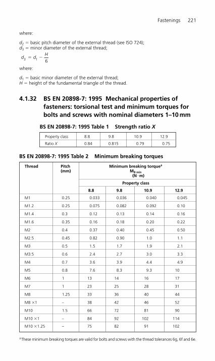
where:
d2 � basic pitch diameter of the external thread (see ISO 724);d3 � minor diameter of the external thread;
where:
d1 � basic minor diameter of the external thread;H � height of the fundamental triangle of the thread.
4.1.32 BS EN 20898-7: 1995 Mechanical properties of fasteners: torsional test and minimum torques forbolts and screws with nominal diameters 1–10 mm
d dH
3 1 6� �
Fastenings 221
Property class 8.8 9.8 10.9 12.9
Ratio X 0.84 0.815 0.79 0.75
BS EN 20898-7: 1995 Table 1 Strength ratio X
BS EN 20898-7: 1995 Table 2 Minimum breaking torques
Thread Pitch Minimum breaking torquea
(mm) MB min(N m)
Property class
8.8 9.8 10.9 12.9
M1 0.25 0.033 0.036 0.040 0.045
M1.2 0.25 0.075 0.082 0.092 0.10
M1.4 0.3 0.12 0.13 0.14 0.16
M1.6 0.35 0.16 0.18 0.20 0.22
M2 0.4 0.37 0.40 0.45 0.50
M2.5 0.45 0.82 0.90 1.0 1.1
M3 0.5 1.5 1.7 1.9 2.1
M3.5 0.6 2.4 2.7 3.0 3.3
M4 0.7 3.6 3.9 4.4 4.9
M5 0.8 7.6 8.3 9.3 10
M6 1 13 14 16 17
M7 1 23 25 28 31
M8 1.25 33 36 40 44
M8 1 – 38 42 46 52
M10 1.5 66 72 81 90
M10 1 – 84 92 102 114
M10 1.25 – 75 82 91 102
aThese minimum breaking torques are valid for bolts and screws with the thread tolerances 6g, 6f and 6e.
H6508-Ch04.1d.qxd 9/21/05 3:12 PM Page 221
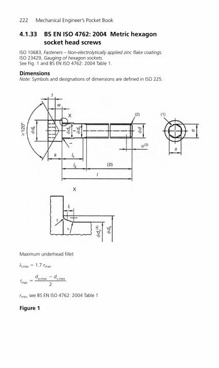
4.1.33 BS EN ISO 4762: 2004 Metric hexagon socket head screws
ISO 10683, Fasteners – Non-electrolytically applied zinc flake coatings.ISO 23429, Gauging of hexagon sockets.See Fig. 1 and BS EN ISO 4762: 2004 Table 1.
DimensionsNote: Symbols and designations of dimensions are defined in ISO 225.
Maximum underhead fillet
lf,max � 1.7 rmax
rmin, see BS EN ISO 4762: 2004 Table 1
Figure 1
rd d
maxa,max s,max�
�
2
222 Mechanical Engineer’s Pocket Book
t
w
�12
0º
fd k
fd a
fd s
(4)
fd a
fd s
fd
k ls
lg
lf
l
(b)
r
r
r
(2) (1)
u (3)s
eX
X
H6508-Ch04.1d.qxd 9/21/05 3:12 PM Page 222

Fastenings 223
t
w
�12
0° r
fd w
fd w
v
v
(6)
(5)
�45°
e/2
(e/2)/3
For broached sockets which are at the maximum limitof size the overcut resulting from drilling shall not exceed1/3 of the length of any flat of the socket which is e/2.
(1) A slight rounding or countersink at the mouth of the socket is permissible.(2) Point chamfered or for sizes M4 and below ‘as rolled’ according to ISO 4753.(3) Incomplete thread u � 2P.(4) ds applies if values of ls,min are specified.(5) Top edge of head may be rounded or chamfered as shown at the option
of the manufacturer.(6) Bottom edge of head may be rounded or chamfered to dw but in every
case shall be free from burrs.
Permissible alternative form of socket Top and bottom edge of the head
Figure 1 continued
H6508-Ch04.1d.qxd 9/21/05 3:12 PM Page 223
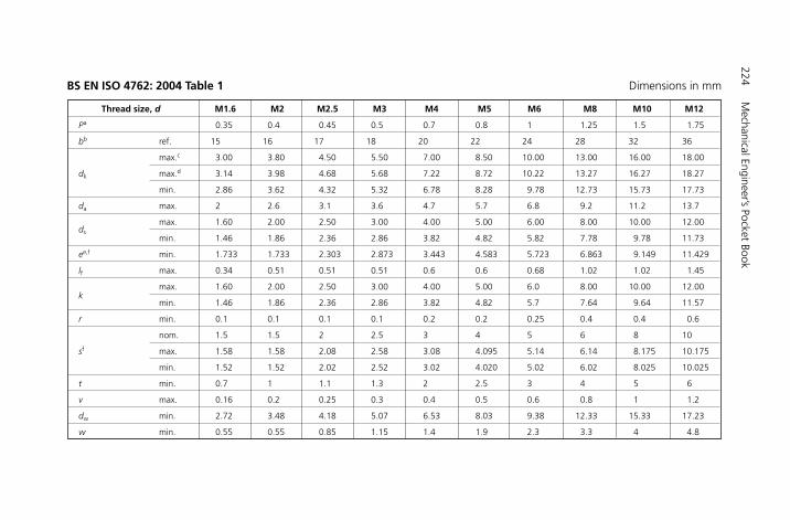
Thread size, d M1.6 M2 M2.5 M3 M4 M5 M6 M8 M10 M12
Pa 0.35 0.4 0.45 0.5 0.7 0.8 1 1.25 1.5 1.75
bb ref. 15 16 17 18 20 22 24 28 32 36
max.c 3.00 3.80 4.50 5.50 7.00 8.50 10.00 13.00 16.00 18.00
dk max.d 3.14 3.98 4.68 5.68 7.22 8.72 10.22 13.27 16.27 18.27
min. 2.86 3.62 4.32 5.32 6.78 8.28 9.78 12.73 15.73 17.73
da max. 2 2.6 3.1 3.6 4.7 5.7 6.8 9.2 11.2 13.7
max. 1.60 2.00 2.50 3.00 4.00 5.00 6.00 8.00 10.00 12.00ds
min. 1.46 1.86 2.36 2.86 3.82 4.82 5.82 7.78 9.78 11.73
ee,f min. 1.733 1.733 2.303 2.873 3.443 4.583 5.723 6.863 9.149 11.429
lf max. 0.34 0.51 0.51 0.51 0.6 0.6 0.68 1.02 1.02 1.45
kmax. 1.60 2.00 2.50 3.00 4.00 5.00 6.0 8.00 10.00 12.00
min. 1.46 1.86 2.36 2.86 3.82 4.82 5.7 7.64 9.64 11.57
r min. 0.1 0.1 0.1 0.1 0.2 0.2 0.25 0.4 0.4 0.6
nom. 1.5 1.5 2 2.5 3 4 5 6 8 10
sf max. 1.58 1.58 2.08 2.58 3.08 4.095 5.14 6.14 8.175 10.175
min. 1.52 1.52 2.02 2.52 3.02 4.020 5.02 6.02 8.025 10.025
t min. 0.7 1 1.1 1.3 2 2.5 3 4 5 6
v max. 0.16 0.2 0.25 0.3 0.4 0.5 0.6 0.8 1 1.2
dw min. 2.72 3.48 4.18 5.07 6.53 8.03 9.38 12.33 15.33 17.23
w min. 0.55 0.55 0.85 1.15 1.4 1.9 2.3 3.3 4 4.8
BS EN ISO 4762: 2004 Table 1 Dimensions in mm
224M
echanical Engineer’s Pocket Book
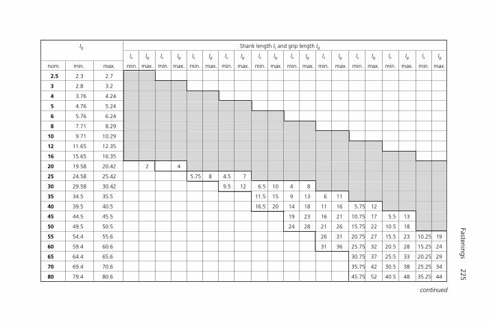
Ig Shank length ls and grip length lg
ls lg ls lg ls lg ls lg ls lg ls lg ls lg ls lg ls lg ls lg
nom. min. max. min. max. min. max. min. max. min. max. min. max. min. max. min. max. min. max. min. max. min. max.
2.5 2.3 2.7
3 2.8 3.2
4 3.76 4.24
5 4.76 5.24
6 5.76 6.24
8 7.71 8.29
10 9.71 10.29
12 11.65 12.35
16 15.65 16.35
20 19.58 20.42 2 4
25 24.58 25.42 5.75 8 4.5 7
30 29.58 30.42 9.5 12 6.5 10 4 8
35 34.5 35.5 11.5 15 9 13 6 11
40 39.5 40.5 16.5 20 14 18 11 16 5.75 12
45 44.5 45.5 19 23 16 21 10.75 17 5.5 13
50 49.5 50.5 24 28 21 26 15.75 22 10.5 18
55 54.4 55.6 26 31 20.75 27 15.5 23 10.25 19
60 59.4 60.6 31 36 25.75 32 20.5 28 15.25 24
65 64.4 65.6 30.75 37 25.5 33 20.25 29
70 69.4 70.6 35.75 42 30.5 38 25.25 34
80 79.4 80.6 45.75 52 40.5 48 35.25 44
Fastenings225
continued

226M
echanical Engineer’s Pocket Book
Ig Shank length ls and grip length lg
ls lg ls lg ls lg ls lg ls lg ls lg ls lg ls lg ls lg ls lg
nom. min. max. min. max. min. max. min. max. min. max. min. max. min. max. min. max. min. max. min. max. min. max.
90 89.3 90.7 50.5 58 45.25 54
100 99.3 100.7 60.5 68 55.25 64
110 109.3 110.7 65.25 74
120 119.3 120.7 75.25 84
130 129.2 130.8
140 139.2 140.8
150 149.2 150.8
160 159.2 160.8
180 179.2 180.8
200 199.075 200.925
220 219.075 220.925
240 239.075 240.925
260 258.95 261.05
280 278.95 281.05
300 298.95 301.05
BS EN ISO 4762: 2004 Table 1 (continued )

Fastenings227
Thread size, d (M14)h M16 M20 M24 M30 M36 M42 M48 M56 M64
Pa 2 2 2.5 3 3.5 4 4.5 5 5.5 6
bb ref. 40 44 52 60 72 84 96 108 124 140
dk max.c 21.00 24.00 30.00 36.00 45.00 54.00 63.00 72.00 84.00 96.00
max.d 21.33 24.33 30.33 36.39 45.39 54.46 63.46 72.46 84.54 96.54
min. 20.67 23.67 29.67 35.61 44.61 53.54 62.54 71.54 83.46 95.46
da max. 15.7 17.7 22.4 26.4 33.4 39.4 45.6 52.6 63 71
ds max. 14.00 16.00 20.00 24.00 30.00 36.00 42.00 48.00 56.00 64.00
min. 13.73 15.73 19.67 23.67 29.67 35.61 41.61 47.61 55.54 63.54
ee,f min. 13.716 15.996 19.437 21.734 25.154 30.854 36.571 41.131 46.831 52.531
lf max. 1.45 1.45 2.04 2.04 2.89 2.89 3.06 3.91 5.95 5.95
k max. 14.00 16.00 20.00 24.00 30.00 36.00 42.00 48.00 56.00 64.00
min. 13.57 15.57 19.48 23.48 29.48 35.38 41.38 47.38 55.26 63.26
r min. 0.6 0.6 0.8 0.8 1 1 1.2 1.6 2 2
sf nom. 12 14 17 19 22 27 32 36 41 46
max. 12.212 14.212 17.23 19.275 22.275 27.275 32.33 36.33 41.33 46.33
min. 12.032 14.032 17.05 19.065 22.065 27.065 32.08 36.08 41.08 46.08
t min. 7 8 10 12 15.5 19 24 28 34 38
v max. 1.4 1.6 2 2.4 3 3.6 4.2 4.8 5.6 6.4
dw min. 20.17 23.17 28.87 34.81 43.61 52.54 61.34 70.34 82.26 94.26
w min. 5.8 6.8 8.6 10.4 13.1 15.3 16.3 17.5 19 22
continued
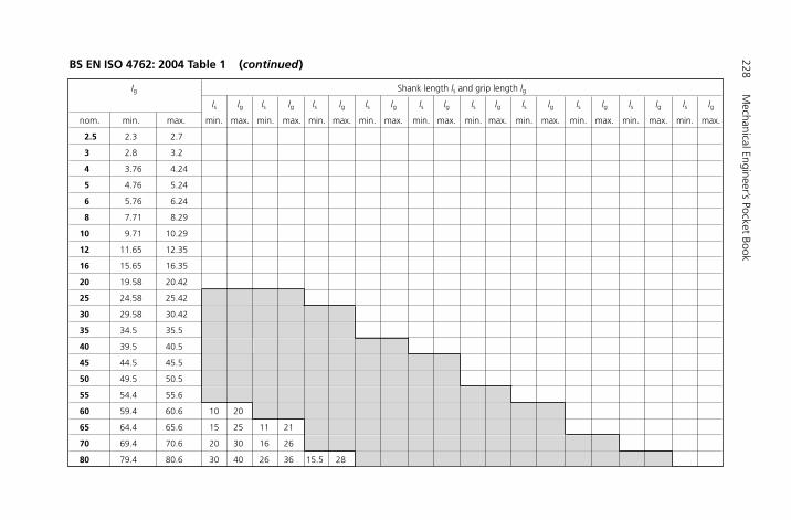
228M
echanical Engineer’s Pocket Book
Ig Shank length ls and grip length lg
ls lg ls lg ls lg ls lg ls lg ls lg ls lg ls lg ls lg ls lg
nom. min. max. min. max. min. max. min. max. min. max. min. max. min. max. min. max. min. max. min. max. min. max.
2.5 2.3 2.7
3 2.8 3.2
4 3.76 4.24
5 4.76 5.24
6 5.76 6.24
8 7.71 8.29
10 9.71 10.29
12 11.65 12.35
16 15.65 16.35
20 19.58 20.42
25 24.58 25.42
30 29.58 30.42
35 34.5 35.5
40 39.5 40.5
45 44.5 45.5
50 49.5 50.5
55 54.4 55.6
60 59.4 60.6 10 20
65 64.4 65.6 15 25 11 21
70 69.4 70.6 20 30 16 26
80 79.4 80.6 30 40 26 36 15.5 28
BS EN ISO 4762: 2004 Table 1 (continued)
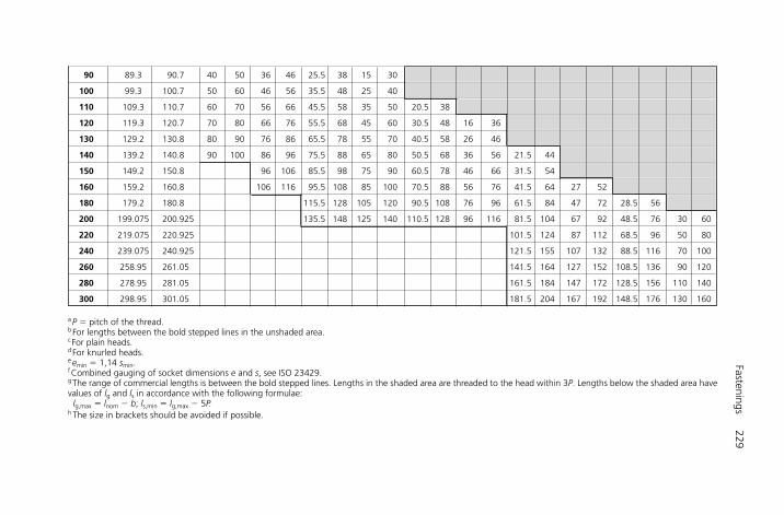
Fastenings229
90 89.3 90.7 40 50 36 46 25.5 38 15 30
100 99.3 100.7 50 60 46 56 35.5 48 25 40
110 109.3 110.7 60 70 56 66 45.5 58 35 50 20.5 38
120 119.3 120.7 70 80 66 76 55.5 68 45 60 30.5 48 16 36
130 129.2 130.8 80 90 76 86 65.5 78 55 70 40.5 58 26 46
140 139.2 140.8 90 100 86 96 75.5 88 65 80 50.5 68 36 56 21.5 44
150 149.2 150.8 96 106 85.5 98 75 90 60.5 78 46 66 31.5 54
160 159.2 160.8 106 116 95.5 108 85 100 70.5 88 56 76 41.5 64 27 52
180 179.2 180.8 115.5 128 105 120 90.5 108 76 96 61.5 84 47 72 28.5 56
200 199.075 200.925 135.5 148 125 140 110.5 128 96 116 81.5 104 67 92 48.5 76 30 60
220 219.075 220.925 101.5 124 87 112 68.5 96 50 80
240 239.075 240.925 121.5 155 107 132 88.5 116 70 100
260 258.95 261.05 141.5 164 127 152 108.5 136 90 120
280 278.95 281.05 161.5 184 147 172 128.5 156 110 140
300 298.95 301.05 181.5 204 167 192 148.5 176 130 160
aP � pitch of the thread.bFor lengths between the bold stepped lines in the unshaded area.cFor plain heads.dFor knurled heads.eemin � 1,14 smin.fCombined gauging of socket dimensions e and s, see ISO 23429.gThe range of commercial lengths is between the bold stepped lines. Lengths in the shaded area are threaded to the head within 3P. Lengths below the shaded area havevalues of lg and ls in accordance with the following formulae:lg,max � lnom � b; ls,min � lg,max � 5P.
h The size in brackets should be avoided if possible.

4.1.34 BS EN ISO 10642: 2004 Hexagon socket countersunkhead screws
Dimensions and gauging of headSee Figs 1 and 2, and BS EN ISO 10642: 2004 Table 1.
DimensionsNote: Symbols and designations of dimensions are defined in ISO 225.
230 Mechanical Engineer’s Pocket Book
k
w
w
fd
(6)
fd
k
fd
t
t
(2)
(3)r
(1)
e
su (5)
(b)
lslg
l
a(4
)
�12
0°
�12
0°
s
Permissible alternative form of socket
Figure 1 Hexagon socket countersunk head screws.
H6508-Ch04.1d.qxd 9/21/05 3:12 PM Page 230
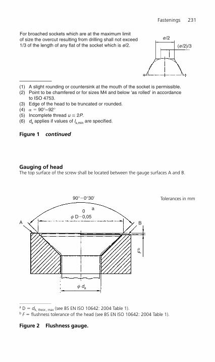
Fastenings 231
Gauging of headThe top surface of the screw shall be located between the gauge surfaces A and B.
90°�0°30'
φ D�0,050
A
a
B
Fb
φ da
a D � dk, theor., max (see BS EN ISO 10642: 2004 Table 1).b F � flushness tolerance of the head (see BS EN ISO 10642: 2004 Table 1).
Figure 2 Flushness gauge.
e /2
(e /2)/3
For broached sockets which are at the maximum limitof size the overcut resulting from drilling shall not exceed1/3 of the length of any flat of the socket which is e/2.
(1) A slight rounding or countersink at the mouth of the socket is permissible.(2) Point to be chamfered or for sizes M4 and below ‘as rolled’ in accordance to ISO 4753.(3) Edge of the head to be truncated or rounded.(4) a � 90°–92°(5) Incomplete thread u � 2P.(6) ds applies if values of ls,min are specified.
Figure 1 continued
Tolerances in mm
H6508-Ch04.1d.qxd 9/21/05 3:12 PM Page 231
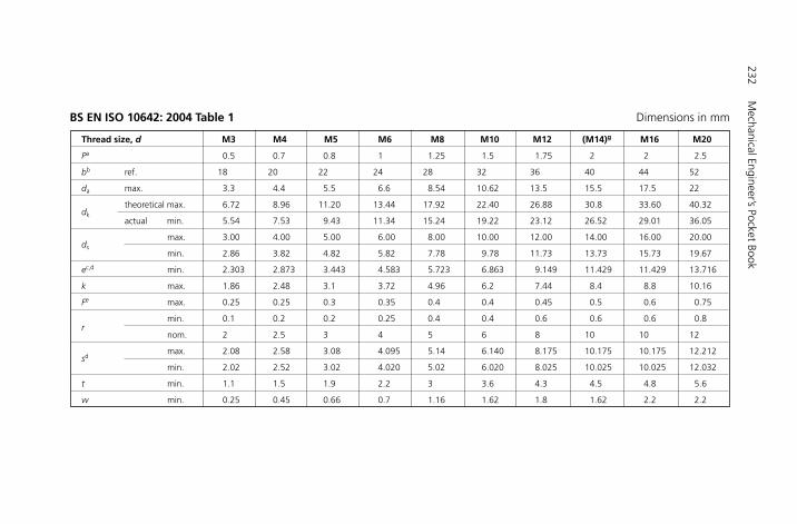
232M
echanical Engineer’s Pocket Book
Thread size, d M3 M4 M5 M6 M8 M10 M12 (M14)g M16 M20
Pa 0.5 0.7 0.8 1 1.25 1.5 1.75 2 2 2.5
bb ref. 18 20 22 24 28 32 36 40 44 52
da max. 3.3 4.4 5.5 6.6 8.54 10.62 13.5 15.5 17.5 22
dk
theoretical max. 6.72 8.96 11.20 13.44 17.92 22.40 26.88 30.8 33.60 40.32
actual min. 5.54 7.53 9.43 11.34 15.24 19.22 23.12 26.52 29.01 36.05
ds
max. 3.00 4.00 5.00 6.00 8.00 10.00 12.00 14.00 16.00 20.00
min. 2.86 3.82 4.82 5.82 7.78 9.78 11.73 13.73 15.73 19.67
ec,d min. 2.303 2.873 3.443 4.583 5.723 6.863 9.149 11.429 11.429 13.716
k max. 1.86 2.48 3.1 3.72 4.96 6.2 7.44 8.4 8.8 10.16
Fe max. 0.25 0.25 0.3 0.35 0.4 0.4 0.45 0.5 0.6 0.75
rmin. 0.1 0.2 0.2 0.25 0.4 0.4 0.6 0.6 0.6 0.8
nom. 2 2.5 3 4 5 6 8 10 10 12
sdmax. 2.08 2.58 3.08 4.095 5.14 6.140 8.175 10.175 10.175 12.212
min. 2.02 2.52 3.02 4.020 5.02 6.020 8.025 10.025 10.025 12.032
t min. 1.1 1.5 1.9 2.2 3 3.6 4.3 4.5 4.8 5.6
w min. 0.25 0.45 0.66 0.7 1.16 1.62 1.8 1.62 2.2 2.2
BS EN ISO 10642: 2004 Table 1 Dimensions in mm
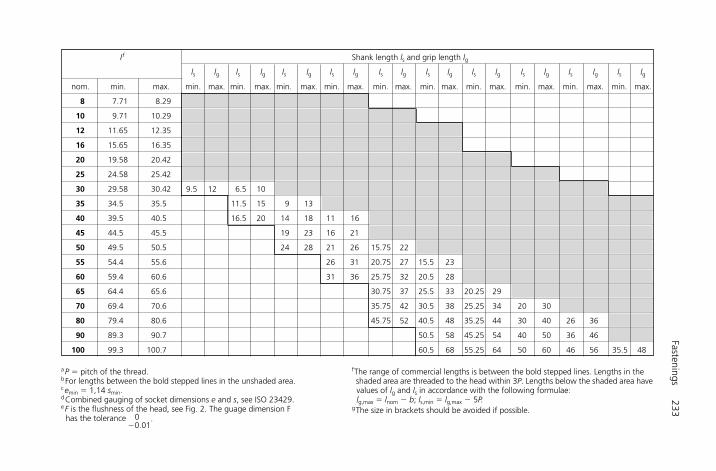
Fastenings233
If Shank length ls and grip length lg
ls lg ls lg ls lg ls lg ls lg ls lg ls lg ls lg ls lg ls lg
nom. min. max. min. max. min. max. min. max. min. max. min. max. min. max. min. max. min. max. min. max. min. max.
8 7.71 8.29
10 9.71 10.29
12 11.65 12.35
16 15.65 16.35
20 19.58 20.42
25 24.58 25.42
30 29.58 30.42 9.5 12 6.5 10
35 34.5 35.5 11.5 15 9 13
40 39.5 40.5 16.5 20 14 18 11 16
45 44.5 45.5 19 23 16 21
50 49.5 50.5 24 28 21 26 15.75 22
55 54.4 55.6 26 31 20.75 27 15.5 23
60 59.4 60.6 31 36 25.75 32 20.5 28
65 64.4 65.6 30.75 37 25.5 33 20.25 29
70 69.4 70.6 35.75 42 30.5 38 25.25 34 20 30
80 79.4 80.6 45.75 52 40.5 48 35.25 44 30 40 26 36
90 89.3 90.7 50.5 58 45.25 54 40 50 36 46
100 99.3 100.7 60.5 68 55.25 64 50 60 46 56 35.5 48
aP � pitch of the thread. fThe range of commercial lengths is between the bold stepped lines. Lengths in thebFor lengths between the bold stepped lines in the unshaded area. shaded area are threaded to the head within 3P. Lengths below the shaded area havecemin � 1,14 smin. values of lg and ls in accordance with the following formulae:dCombined gauging of socket dimensions e and s, see ISO 23429. lg,max � lnom � b; ls,min � lg,max � 5P.eF is the flushness of the head, see Fig. 2. The guage dimension F gThe size in brackets should be avoided if possible.has the tolerance 0
�0.01.
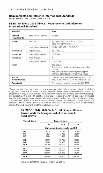
234 Mechanical Engineer’s Pocket Book
Requirements and reference International StandardsSee BS EN ISO 10642: 2004 Tables 2 and 3.
Material Steel
General International Standard ISO 8992requirements
Thread Tolerance 6g for property classes 8.8 and 10.9;5g6g for property class 12.9
International Standards ISO 261, ISO 965-2, ISO 965-3
Mechanical Property classa 8.8, 10.9, 12.9
properties International Standard ISO 898-1
Tolerances Product grade A
International Standard ISO 4759-1
Finish As processedRequirements for electroplating are covered inISO 4042Requirements for non-electrolytically appliedzinc flake coatings are covered in ISO 10683
Surface Limits for surface discontinuities are given in ISOdiscontinuities 6157-1 and ISO 6157-3 for property class 12.9
Acceptability Acceptance procedure is covered in ISO 3269
BS EN ISO 10642: 2004 Table 2 Requirements and referenceInternational Standards
BS EN ISO 10642: 2004 Table 3 Minimum ultimatetensile loads for hexagon socket countersunkhead screws
Thread size, d Property class
8.8 10.9 12.9
Minimum ultimate tensile load (N)
M3 3 220 4 180 4 190M4 5 620 7 300 8 560M5 9 080 11 800 13 800
M6 12 900 16 700 19 600M8 23 400 30 500 35 700M10 37 100 48 200 56 600
M12 53 900 70 200 82 400M14 73 600 96 000 112 000M16 100 000 130 000 154 000
M20 162 000 204 000 239 000
Eighty per cent of the values specified in ISO 898-1.
aBecause of their head configurations, these screws may not meet the minimum ultimate tensile loadfor property classes 8.8, 10.9 and 12.9, specified in ISO 898-1, when tested in accordance with testprogramme B. They shall nevertheless meet the other material and property requirements for prop-erty classes 8.8, 10.9 and 12.9 specified in ISO 898-1. In addition, when full-size screws are loadedwith the head supported on a suitable collar (conical bearing surface) using the type of testing fixtureillustrated in ISO 898-1, they shall withstand, without fracture, the minimum ultimate tensile loadsgiven in BS EN ISO 10642: 2004 Table 3. If tested to failure, the fracture may occur in the threadedsection, the head, the shank or at the head/shank junction.
H6508-Ch04.1d.qxd 9/21/05 3:12 PM Page 234
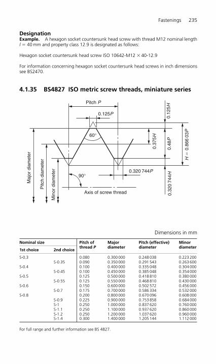
Fastenings 235
DesignationExample. A hexagon socket countersunk head screw with thread M12 nominal lengthl � 40 mm and property class 12.9 is designated as follows:
Hexagon socket countersunk head screw ISO 10642-M12 � 40-12.9
For information concerning hexagon socket countersunk head screws in inch dimensionssee BS2470.
4.1.35 BS4827 ISO metric screw threads, miniature series
Axis of screw thread
Pitch P
0.125P
0.37
5H
0.12
5H
H �
0.8
6603
P
0.32
074
4H0.320 744P
0.48
P
60°
90°
Min
or d
iam
eter
Pitc
h di
amet
er
Maj
or d
iam
eter
Dimensions in mm
Nominal size Pitch of Major Pitch (effective) Minor
1st choice 2nd choicethread P diameter diameter diameter
S-0.3 0.080 0.300 000 0.248 038 0.223 200S-0.35 0.090 0.350 000 0.291 543 0.263 600
S-0.4 0.100 0.400 000 0.335 048 0.304 000S-0.45 0.100 0.450 000 0.385 048 0.354 000
S-0.5 0.125 0.500 000 0.418 810 0.380 000S-0.55 0.125 0.550 000 0.468 810 0.430 000
S-0.6 0.150 0.600 000 0.502 572 0.456 000S-0.7 0.175 0.700 000 0.586 334 0.532 000
S-0.8 0.200 0.800 000 0.670 096 0.608 000S-0.9 0.225 0.900 000 0.753 858 0.684 000S-1 0.250 1.000 000 0.837 620 0.760 000S-1.1 0.250 1.100 000 0.937 620 0.860 000S-1.2 0.250 1.200 000 1.037 620 0.960 000S-1.4 0.300 1.400 000 1.205 144 1.112 000
For full range and further information see BS 4827.
H6508-Ch04.1e.qxd 9/12/05 4:41 PM Page 235
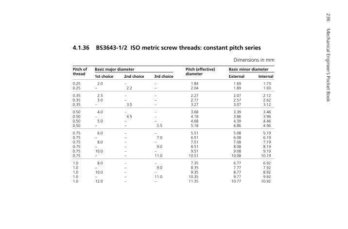
4.1.36 BS3643-1/2 ISO metric screw threads: constant pitch series
236M
echanical Engineer’s Pocket Book
Dimensions in mm
Pitch of Basic major diameter Pitch (effective) Basic minor diameterthread
1st choice 2nd choice 3rd choicediameter
External Internal
0.25 2.0 – – 1.84 1.69 1.730.25 – 2.2 – 2.04 1.89 1.93
0.35 2.5 – – 2.27 2.07 2.120.35 3.0 – – 2.77 2.57 2.620.35 – 3.5 – 3.27 3.07 3.12
0.50 4.0 – – 3.68 3.39 3.460.50 – 4.5 – 4.18 3.86 3.960.50 5.0 – – 4.68 4.39 4.460.50 – – 5.5 5.18 4.86 4.96
0.75 6.0 – – 5.51 5.08 5.190.75 – – 7.0 6.51 6.08 6.190.75 8.0 – – 7.51 7.08 7.190.75 – – 9.0 8.51 8.08 8.190.75 10.0 – – 9.51 9.08 9.190.75 – – 11.0 10.51 10.08 10.19
1.0 8.0 – – 7.35 6.77 6.921.0 – – 9.0 8.35 7.77 7.921.0 10.0 – – 9.35 8.77 8.921.0 – – 11.0 10.35 9.77 9.921.0 12.0 – – 11.35 10.77 10.92

Fastenings237
1.0 – 14.0 – 13.35 12.77 12.921.0 – – 15.0 14.35 13.77 13.921.0 16.0 – – 15.35 14.77 14.921.0 – – 17.0 16.35 15.77 15.921.0 – 18.0 – 17.35 16.77 16.921.0 20.0 – – 19.35 18.77 18.921.0 – 22.0 – 21.35 21.77 21.921.0 24.0 – – 23.35 22.77 22.921.0 – – 25.0 24.35 23.77 23.921.0 – 27.0 – 26.35 25.77 25.921.0 – – 28.0 27.35 26.77 26.921.0 30.0 – – 29.35 28.77 28.92
1.25 10.0 – – 9.19 8.47 8.651.25 12.0 – – 11.19 10.47 10.651.25a – 14.0a – 13.19 12.47 12.65
1.5 12.0 – – 11.03 10.16 10.381.5 – 14.0 – 13.03 12.16 12.381.5 – – 15.0 14.03 13.16 13.381.5 16.0 – – 15.03 14.16 14.381.5 – – 17.0 16.03 15.16 15.381.5 – 18.0 – 17.03 16.16 16.381.5 20.0 – – 19.03 18.16 18.381.5 – 22.0 – 21.03 20.16 20.381.5 24.0 – – 23.03 22.16 22.381.5 – – 25.0 24.03 23.16 23.381.5 – – 26.0 25.03 24.16 24.381.5 – 27.0 – 26.03 25.16 25.381.5 – – 28.0 27.03 26.16 26.381.5 30.0 – – 29.03 28.16 28.38
continued

238M
echanical Engineer’s Pocket Book
Section 4.1.36 (continued ) Dimensions in mm
Pitch of Basic major diameter Pitch (effective) Basic minor diameterthread
1st choice 2nd choice 3rd choicediameter
External Internal
1.5 – – 32.0 31.03 30.16 30.381.5 – 33.0 – 32.03 31.16 31.381.5 – – 35.0 34.03 33.16 33.38The 1.5 mm pitch series continues to a maximum diameter of 80 mm
2.0 – 18.0 – 16.70 15.55 15.842.0 20.0 – – 18.70 17.55 17.842.0 – 22.0 – 20.70 19.55 19.842.0 24.0 – – 22.70 21.55 21.842.0 – – 25.0 23.70 22.55 22.842.0 – – 26.0 24.70 23.55 23.842.0 – 27.0 – 25.70 24.55 24.842.0 – – 28.0 26.70 25.55 25.842.0 30.0 – – 28.70 27.55 27.842.0 – – 32.0 30.70 29.55 29.842.0 – 33.0 – 31.70 30.55 30.842.0 – – 35.0 33.70 32.55 32.84The 2.0 mm pitch series continues to a maximum diameter of 150 mm
3.0 30.0 – – 28.05 26.32 26.753.0 – 33.0 – 31.05 29.32 29.753.0 36.0 – – 34.05 32.32 32.753.0 – – 38.0 36.05 34.32 34.753.0 – 39.0 – 37.05 35.32 35.753.0 – – 40.0 38.05 36.32 36.753.0 42.0 – – 40.05 38.32 38.753.0 – 45.0 – 43.05 41.32 41.753.0 48.0 – – 46.05 44.32 44.75

Fastenings239
3.0 – – 50.0 48.05 46.32 46.753.0 – 52.0 – 50.05 48.32 48.753.0 – – 55.0 53.05 51.32 51.75The 3.0 mm pitch series continues to a maximum diameter of 250 mm
4.0 42.0 – – 39.40 37.09 37.674.0 – 45.0 – 42.40 40.09 40.674.0 48.0 – – 45.40 43.09 43.674.0 – – 50.0 47.40 45.09 45.674.0 – 52.0 – 49.40 47.09 47.674.0 – – 55.0 52.40 50.09 50.674.0 56.0 – – 53.40 51.09 51.674.0 – – 58.0 55.40 53.09 53.674.0 – 60.0 – 57.40 55.09 55.674.0 – – 62.0 59.40 57.09 57.674.0 64.0 – – 61.40 59.09 59.674.0 – – 65.0 62.40 60.09 60.67The 4.0 mm pitch series continues to a maximum diameter of 300 mm
6.0 – – 70.0 66.10 62.64 63.506.0 72.0 – – 68.10 64.64 65.506.0 – 76.0 – 72.10 68.64 69.506.0 80.0 – – 76.10 72.64 73.506.0 – 85.0 – 81.10 77.64 78.506.0 90.0 – – 86.10 82.64 83.506.0 – 95.0 – 91.10 87.64 88.506.0 100.0 – – 96.10 92.64 93.506.0 – 105.0 – 101.10 97.64 98.506.0 110.0 – – 106.10 102.64 103.506.0 – 115.0 – 111.10 107.64 108.506.0 – 120.0 – 116.10 112.64 113.506.0 125.0 – – 121.10 117.64 118.50The 6.0 mm pitch series continues to a maximum diameter of 300 mm
aThis size sparking plugs only.For further information see BS 3643.

4.1.37 BS EN ISO 228-1: 2003 Pipe threads where pressure-tight joints are not made on the threads
Part 1: Dimensions, tolerances and designationScopeThis part of ISO 228 specifies the requirements for thread form, dimensions, tolerancesand designation for fastening pipe threads, thread sizes 1/16 to 6 inclusive. Both internaland external threads are parallel threads, intended for the mechanical assembly of thecomponent parts of fittings, cocks and valves, accessories, etc.
These threads are not suitable as jointing threads where a pressure-tight joint is made onthe thread. If assemblies with such threads must be made pressure-tight, this should beeffected by compressing two tightening surfaces outside the threads, and by interposingand appropriate seal.
Notes:● For pipe threads where pressure-tight joints are made on the threads, see ISO 7-1.● ISO 228-2 gives details of methods for verification of fastening thread dimensions and
form, and recommended gauging systems.
Normative referenceThe following normative document contains provisions which, through reference in thistext, constitute provisions of this part of ISO 228. For dated references, subsequentamendments to, or revisions of, any of these publications do not apply. However, partiesto agreements based on this part of ISO 228 are encouraged to investigate the possibilityof applying the most recent editions of the normative document indicated below. Forundated references, the latest edition of the normative document referred to applies.Members of ISO and IEC maintain registers of currently valid International Standards.
ISO 7-1:1994, Pipe threads where pressure-tight joints are made on the threads – Part 1:Dimensions, tolerances and designation.
SymbolsFor the purposes of this part of ISO 228, the following symbols apply:
A Tighter class of tolerance of external pipe threads where pressure-tight joints are notmade on the threads.
B Wider class of tolerance of external pipe threads where pressure-tight joints are notmade on the threads.
D � d; major diameter of the internal thread.D1 � D � 1,280 654 P � d1; minor diameter of the internal thread.D2 � D � 0,640 327 P � d2; pitch diameter of the internal thread.d Major diameter of the external thread.d1 � d � 1,280 654 P; minor diameter of the external thread.d2 � d � 0,640 327 P; pitch diameter of the external thread.G Pipe thread where pressure-tight joints are not made on the threads.H Height of the fundamental triangle of the thread.h Height of the thread profile with rounded crests and roots.P Pitch.r Radius of rounded crests and roots.TD1 Tolerance on the minor diameter of the internal thread.TD2 Tolerance on the pitch diameter of the internal thread.Td Tolerance on the major diameter of the external thread.Td2 Tolerance on the pitch diameter of the external thread.
240 Mechanical Engineer’s Pocket Book
H6508-Ch04.1e.qxd 9/12/05 4:41 PM Page 240
DimensionsThe profile of these threads is identical with that of the parallel thread specified in ISO 7-1. The internal and external threads covered by this part of ISO 228 are both parallel.
Unless otherwise specified, the thread in accordance with this part of ISO 228 is a right-hand thread. (See also clause 5.)
Threads are normally of the truncated form, with crests truncated to the limits of toler-ance as given in columns 14 and 15 of BS EN ISO 228-1: 2003 Table 1. The exception tothis is on internal threads, where they are likely to be assembled with external threads inaccordance with ISO 7-1, and in which case the thread length shall be equal to or greaterthan that specified in ISO 7-1.
The tolerances on the pitch diameter of the internal threads correspond to the positivedeviation of the diameter tolerances in ISO 7-1, with the exception of those for threadsizes 1/16, 1/8, 1/4 and 3/8, for which slightly higher values are specified.
For external threads, two classes of tolerances on the pitch diameter are specified (see BS EN ISO 228-1: 2003 Table 1).
● Class A (column 10) consists of entirely negative tolerances, each equivalent in value tothe tolerance for the respective internal thread.
● Class B (column 11) consists of entirely negative tolerances, each with a value of twicethat of the respective internal thread.
The choice between class A and class B depends on the conditions of application and shallbe made in product standards where threads in accordance with this part of ISO 228 arespecified.
Pipe thread dimensions, in millimetres, are given in BS EN ISO 228-1: 2003 Table 1.
Fig. 1 shows fastening threads with full-form profiles and their tolerance zones.
Fig. 2 shows fastening threads with truncated profiles and their tolerance zones.
Fastenings 241
H6508-Ch04.1e.qxd 9/12/05 4:41 PM Page 241
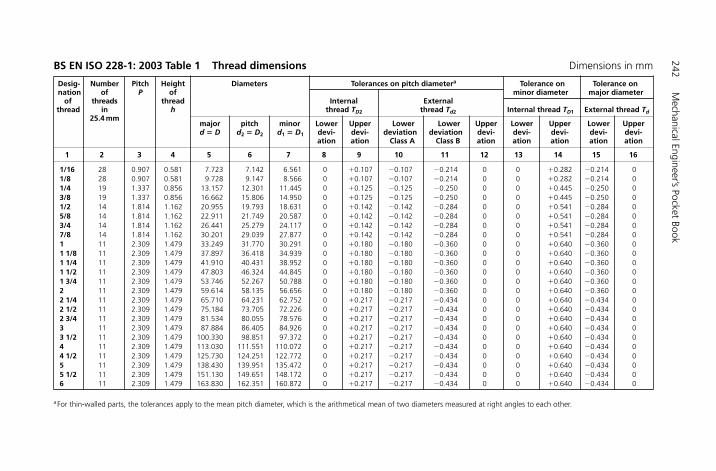
242M
echanical Engineer’s Pocket Book
BS EN ISO 228-1: 2003 Table 1 Thread dimensions Dimensions in mm
Desig- Number Pitch Height Diameters Tolerances on pitch diametera Tolerance on Tolerance on nation of P of minor diameter major diameter
of threads thread Internal External thread in h thread TD2 thread Td2 Internal thread TD1 External thread Td
25.4 mmmajor pitch minor Lower Upper Lower Lower Upper Lower Upper Lower Upper d � D d2 � D2 d1 � D1 devi- devi- deviation deviation devi- devi- devi- devi- devi-
ation ation Class A Class B ation ation ation ation ation
1 2 3 4 5 6 7 8 9 10 11 12 13 14 15 16
1/16 28 0.907 0.581 7.723 7.142 6.561 0 �0.107 �0.107 �0.214 0 0 �0.282 �0.214 01/8 28 0.907 0.581 9.728 9.147 8.566 0 �0.107 �0.107 �0.214 0 0 �0.282 �0.214 01/4 19 1.337 0.856 13.157 12.301 11.445 0 �0.125 �0.125 �0.250 0 0 �0.445 �0.250 03/8 19 1.337 0.856 16.662 15.806 14.950 0 �0.125 �0.125 �0.250 0 0 �0.445 �0.250 01/2 14 1.814 1.162 20.955 19.793 18.631 0 �0.142 �0.142 �0.284 0 0 �0.541 �0.284 05/8 14 1.814 1.162 22.911 21.749 20.587 0 �0.142 �0.142 �0.284 0 0 �0.541 �0.284 03/4 14 1.814 1.162 26.441 25.279 24.117 0 �0.142 �0.142 �0.284 0 0 �0.541 �0.284 07/8 14 1.814 1.162 30.201 29.039 27.877 0 �0.142 �0.142 �0.284 0 0 �0.541 �0.284 01 11 2.309 1.479 33.249 31.770 30.291 0 �0.180 �0.180 �0.360 0 0 �0.640 �0.360 01 1/8 11 2.309 1.479 37.897 36.418 34.939 0 �0.180 �0.180 �0.360 0 0 �0.640 �0.360 01 1/4 11 2.309 1.479 41.910 40.431 38.952 0 �0.180 �0.180 �0.360 0 0 �0.640 �0.360 01 1/2 11 2.309 1.479 47.803 46.324 44.845 0 �0.180 �0.180 �0.360 0 0 �0.640 �0.360 01 3/4 11 2.309 1.479 53.746 52.267 50.788 0 �0.180 �0.180 �0.360 0 0 �0.640 �0.360 02 11 2.309 1.479 59.614 58.135 56.656 0 �0.180 �0.180 �0.360 0 0 �0.640 �0.360 02 1/4 11 2.309 1.479 65.710 64.231 62.752 0 �0.217 �0.217 �0.434 0 0 �0.640 �0.434 02 1/2 11 2.309 1.479 75.184 73.705 72.226 0 �0.217 �0.217 �0.434 0 0 �0.640 �0.434 02 3/4 11 2.309 1.479 81.534 80.055 78.576 0 �0.217 �0.217 �0.434 0 0 �0.640 �0.434 03 11 2.309 1.479 87.884 86.405 84.926 0 �0.217 �0.217 �0.434 0 0 �0.640 �0.434 03 1/2 11 2.309 1.479 100.330 98.851 97.372 0 �0.217 �0.217 �0.434 0 0 �0.640 �0.434 04 11 2.309 1.479 113.030 111.551 110.072 0 �0.217 �0.217 �0.434 0 0 �0.640 �0.434 04 1/2 11 2.309 1.479 125.730 124.251 122.772 0 �0.217 �0.217 �0.434 0 0 �0.640 �0.434 05 11 2.309 1.479 138.430 139.951 135.472 0 �0.217 �0.217 �0.434 0 0 �0.640 �0.434 05 1/2 11 2.309 1.479 151.130 149.651 148.172 0 �0.217 �0.217 �0.434 0 0 �0.640 �0.434 06 11 2.309 1.479 163.830 162.351 160.872 0 �0.217 �0.217 �0.434 0 0 �0.640 �0.434 0
aFor thin-walled parts, the tolerances apply to the mean pitch diameter, which is the arithmetical mean of two diameters measured at right angles to each other.
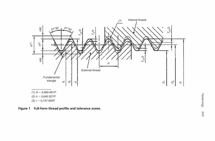
Fastenings243
H/6
Td
2/2
Td/2
TD
1/2
P
D1
D2
Dd 1 d 2 d
TD
2/2
r (3)
h(2)
H(1
)
H/6
27°30� 27°30�
External thread
Internal thread
Fundamentaltriangle
(1) H � 0,960 491P.
(2) h � 0,640 327P.
(3) r � 0,137 329P.
Figure 1 Full-form thread profile and tolerance zones.
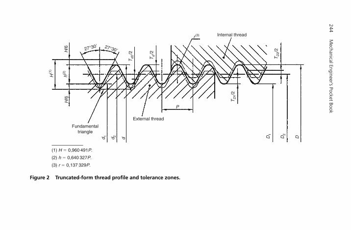
244M
echanical Engineer’s Pocket Book
H/6
Td
2/2
Td/2
TD
1/2
P
D1
D2
Dd 1 d 2 d
TD
2/2
r (3)
h(2)
H(1
)
H/6
27°30� 27°30�
External thread
Internal thread
Fundamentaltriangle
(1) H � 0,960 491P.
(2) h � 0,640 327P.
(3) r � 0,137 329P.
Figure 2 Truncated-form thread profile and tolerance zones.
DesignationThe designation of threads shall consist of the following elements in the given sequence:
(a) Description block: pipe thread.(b) International Standard number block: ISO 228.(c) Individual item block (one of the following, as applicable):
– the letter G followed by the designation of the thread size from column 1 of BS ENISO 228-1: 2003 Table 1 for internal threads (one class of tolerance only); or
– the letter G followed by the designation of the thread size from column 1 of BS ENISO 228-1: 2003 Table 1 and the letter A for class A external threads; or
– the letter G followed by the designation of the thread size from column 1 of BS ENISO 228-1: 2003 Table 1 and the letter B for class B external threads.
(d) For left-hand threads, the letters LH shall be added to the designation. Right-handthreads require no special designation.
Examples. Complete designation for a right-hand thread size 1 1/2:
● Internal thread (one tolerance class only) Pipe thread ISO 228 – G 1 1/2● External thread tolerance class A Pipe thread ISO 228 – G 1 1/2 A
tolerance class B Pipe thread ISO 228 – G 1 1/2 B
Combination with jointing threadCombining an external parallel thread G, tolerance class A or B, in accordance with ISO 228-1, with an internal parallel thread Rp, in accordance with ISO 7-1, needs specialconsideration.
When this combination is necessary, the tolerance of the internal thread in accordancewith ISO 7-1 shall be considered in the relevant product standards, where external parallel threads G are used.
Note:Such a combination of threads does not necessarily achieve a leaktight joint.
Fastenings 245
�
H6508-Ch04.1e.qxd 9/12/05 4:41 PM Page 245
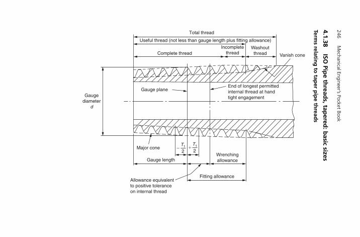
4.1.38ISO
Pipe th
reads, tap
ered: b
asic sizes
Terms relatin
g to
taper p
ipe th
reads
246M
echanical Engineer’s Pocket Book
Allowance equivalentto positive toleranceon internal thread
Major cone
Gauge lengthWrenchingallowance
End of longest permittedinternal thread at handtight engagement
Fitting allowance
Gauge plane
Complete threadIncomplete
threadWashoutthread Vanish cone
Useful thread (not less than gauge length plus fitting allowance)
Gaugediameter
d
Total thread
T1
2�
T1
2�
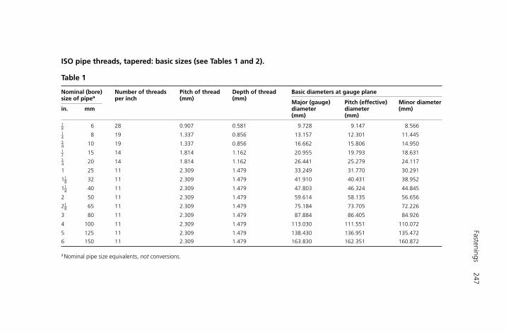
Fastenings247
Table 1
Nominal (bore) Number of threads Pitch of thread Depth of thread Basic diameters at gauge planesize of pipea per inch (mm) (mm)
Major (gauge) Pitch (effective) Minor diameterin. mm diameter diameter (mm)
(mm) (mm)1–8 6 28 0.907 0.581 9.728 9.147 8.5661–4 8 19 1.337 0.856 13.157 12.301 11.4453–8 10 19 1.337 0.856 16.662 15.806 14.9501–2 15 14 1.814 1.162 20.955 19.793 18.6313–4 20 14 1.814 1.162 26.441 25.279 24.117
1 25 11 2.309 1.479 33.249 31.770 30.291
11–8 32 11 2.309 1.479 41.910 40.431 38.952
11–8 40 11 2.309 1.479 47.803 46.324 44.845
2 50 11 2.309 1.479 59.614 58.135 56.656
21–8 65 11 2.309 1.479 75.184 73.705 72.226
3 80 11 2.309 1.479 87.884 86.405 84.926
4 100 11 2.309 1.479 113.030 111.551 110.072
5 125 11 2.309 1.479 138.430 136.951 135.472
6 150 11 2.309 1.479 163.830 162.351 160.872
aNominal pipe size equivalents, not conversions.
ISO pipe threads, tapered: basic sizes (see Tables 1 and 2).
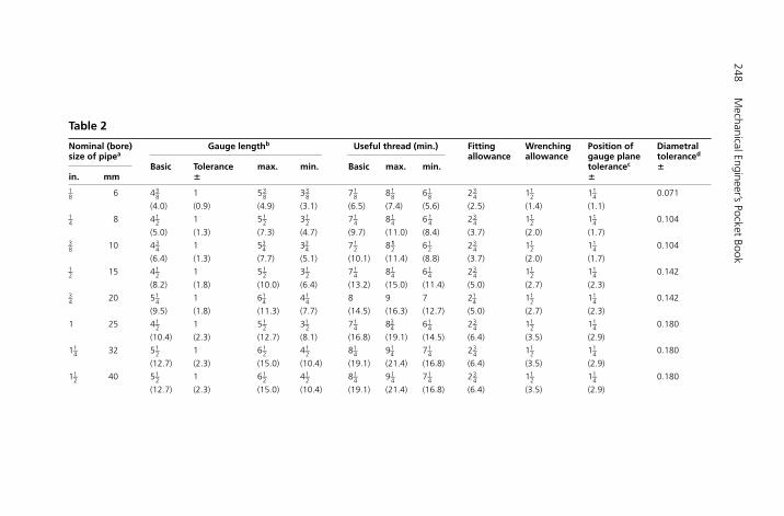
248M
echanical Engineer’s Pocket Book
Table 2
Nominal (bore) Gauge lengthb Useful thread (min.) Fitting Wrenching Position of Diametral size of pipea allowance allowance gauge plane toleranced
Basic Tolerance max. min. Basic max. min. tolerancec �in. mm � �
1–8 6 43–8 1 53–8 33–8 71–8 81–8 61–8 23–4 11–2 11–4 0.071
(4.0) (0.9) (4.9) (3.1) (6.5) (7.4) (5.6) (2.5) (1.4) (1.1)1–4 8 41–2 1 51–2 31–2 71–4 81–4 61–4 23–4 11–2 11–4 0.104
(5.0) (1.3) (7.3) (4.7) (9.7) (11.0) (8.4) (3.7) (2.0) (1.7)3–8 10 43–4 1 53–4 33–4 71–2 811–2 61–2 23–4 11–2 11–4 0.104
(6.4) (1.3) (7.7) (5.1) (10.1) (11.4) (8.8) (3.7) (2.0) (1.7)1–2 15 41–2 1 51–2 31–2 71–4 81–4 61–4 23–4 11–2 11–4 0.142
(8.2) (1.8) (10.0) (6.4) (13.2) (15.0) (11.4) (5.0) (2.7) (2.3)3–4 20 51–4 1 61–4 41–4 8 9 7 21–4 11–2 11–4 0.142
(9.5) (1.8) (11.3) (7.7) (14.5) (16.3) (12.7) (5.0) (2.7) (2.3)
1 25 41–2 1 51–2 31–2 71–4 83–4 61–4 23–4 11–2 11–4 0.180
(10.4) (2.3) (12.7) (8.1) (16.8) (19.1) (14.5) (6.4) (3.5) (2.9)
11–4 32 51–2 1 61–2 41–2 81–4 91–4 71–4 23–4 11–2 11–4 0.180
(12.7) (2.3) (15.0) (10.4) (19.1) (21.4) (16.8) (6.4) (3.5) (2.9)
11–2 40 51–2 1 61–2 41–2 81–4 91–4 71–4 23–4 11–2 11–4 0.180
(12.7) (2.3) (15.0) (10.4) (19.1) (21.4) (16.8) (6.4) (3.5) (2.9)
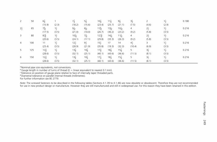
Fastenings249
2 50 67–8 1 77–8 57–8 101–8 111–8 91–8 31–4 2 11–4 0.180
(15.9) (2.3) (18.2) (15.6) (23.4) (25.7) (21.1) (7.5) (4.6) (2.9)
21–2 65 79–-16 11–2 91–-16 61–-16 119–-16 131–-16 101–-16 4 21–2 11–2 0.216
(17.5) (3.5) (21.0) (14.0) (26.7) (30.2) (23.2) (9.2) (5.8) (3.5)
3 80 815–-16 11–2 107–-16 77–-16 1215–-16 147–-16 117–-16 4 21–2 11–2 0.216
(20.6) (3.5) (24.1) (17.1) (29.8) (33.3) (26.3) (9.2) (5.8) (3.5)
4 100 11 11–2 121–2 91–2 151–2 17 14 41–2 3 11–2 0.216
(25.4) (3.5) (28.9) (21.9) (35.8) (19.3) (32.3) (10.4) (6.9) (3.5)
5 125 123–8 11–2 137–8 107–8 173–8 187–8 157–8 5 31–2 11–2 0.216
(28.6) (3.5) (32.1) (25.1) (40.1) (43.6) (36.6) (11.5) (8.1) (3.5)
6 150 123–8 11–2 137–8 107–8 177–8 187–8 157–8 5 31–2 11–2 0.216
(28.6) (3.5) (32.1) (25.1) (40.1) (43.6) (36.6) (11.5) (8.1) (3.5)
aNominal pipe size equivalents, not conversions.bGauge length in number of turns of thread {() � linear equivalent to nearest 0.1 mm}.cTolerance on position of gauge plane relative to face of internally taper threaded parts.dDiametral tolerance on parallel internal threads (millimetres).For further information see BS 2779.
Note: The screwed fasteners to be described in the following tables (Sections 4.1.39 to 4.1.46) are now obsolete or obsolescent. Therefore they are not recommendedfor use in new product design or manufacture. However they are still manufactured and still in widespread use. For this reason they have been retained in this edition.
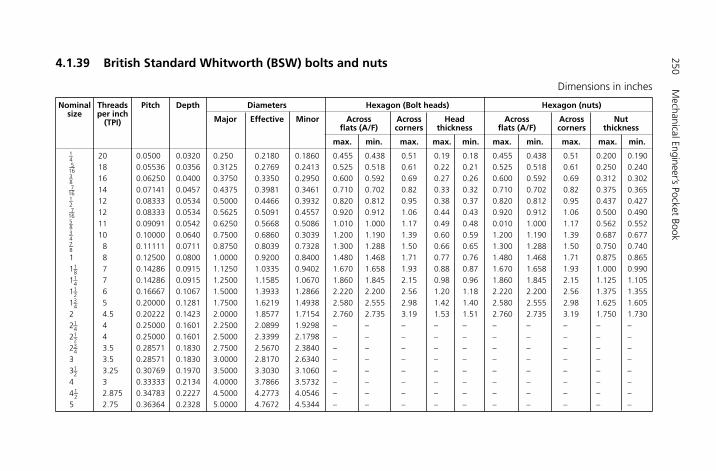
250M
echanical Engineer’s Pocket Book
Dimensions in inches
Nominal Threads Pitch Depth Diameters Hexagon (Bolt heads) Hexagon (nuts)size per inch
Major Effective Minor Across Across Head Across Across Nut (TPI)flats (A/F) corners thickness flats (A/F) corners thickness
max. min. max. max. min. max. min. max. max. min.1–4 20 0.0500 0.0320 0.250 0.2180 0.1860 0.455 0.438 0.51 0.19 0.18 0.455 0.438 0.51 0.200 0.1905–-16 18 0.05536 0.0356 0.3125 0.2769 0.2413 0.525 0.518 0.61 0.22 0.21 0.525 0.518 0.61 0.250 0.2403–8 16 0.06250 0.0400 0.3750 0.3350 0.2950 0.600 0.592 0.69 0.27 0.26 0.600 0.592 0.69 0.312 0.3027–-16 14 0.07141 0.0457 0.4375 0.3981 0.3461 0.710 0.702 0.82 0.33 0.32 0.710 0.702 0.82 0.375 0.3651–2 12 0.08333 0.0534 0.5000 0.4466 0.3932 0.820 0.812 0.95 0.38 0.37 0.820 0.812 0.95 0.437 0.4277–-16 12 0.08333 0.0534 0.5625 0.5091 0.4557 0.920 0.912 1.06 0.44 0.43 0.920 0.912 1.06 0.500 0.4905–8 11 0.09091 0.0542 0.6250 0.5668 0.5086 1.010 1.000 1.17 0.49 0.48 0.010 1.000 1.17 0.562 0.5523–4 10 0.10000 0.0640 0.7500 0.6860 0.3039 1.200 1.190 1.39 0.60 0.59 1.200 1.190 1.39 0.687 0.6777–8 8 0.11111 0.0711 0.8750 0.8039 0.7328 1.300 1.288 1.50 0.66 0.65 1.300 1.288 1.50 0.750 0.7401 8 0.12500 0.0800 1.0000 0.9200 0.8400 1.480 1.468 1.71 0.77 0.76 1.480 1.468 1.71 0.875 0.86511–8 7 0.14286 0.0915 1.1250 1.0335 0.9402 1.670 1.658 1.93 0.88 0.87 1.670 1.658 1.93 1.000 0.99011–4 7 0.14286 0.0915 1.2500 1.1585 1.0670 1.860 1.845 2.15 0.98 0.96 1.860 1.845 2.15 1.125 1.10511–2 6 0.16667 0.1067 1.5000 1.3933 1.2866 2.220 2.200 2.56 1.20 1.18 2.220 2.200 2.56 1.375 1.35513–4 5 0.20000 0.1281 1.7500 1.6219 1.4938 2.580 2.555 2.98 1.42 1.40 2.580 2.555 2.98 1.625 1.6052 4.5 0.20222 0.1423 2.0000 1.8577 1.7154 2.760 2.735 3.19 1.53 1.51 2.760 2.735 3.19 1.750 1.73021–4 4 0.25000 0.1601 2.2500 2.0899 1.9298 – – – – – – – – – –21–2 4 0.25000 0.1601 2.5000 2.3399 2.1798 – – – – – – – – – –23–4 3.5 0.28571 0.1830 2.7500 2.5670 2.3840 – – – – – – – – – –3 3.5 0.28571 0.1830 3.0000 2.8170 2.6340 – – – – – – – – – –31–2 3.25 0.30769 0.1970 3.5000 3.3030 3.1060 – – – – – – – – – –4 3 0.33333 0.2134 4.0000 3.7866 3.5732 – – – – – – – – – –41–2 2.875 0.34783 0.2227 4.5000 4.2773 4.0546 – – – – – – – – – –5 2.75 0.36364 0.2328 5.0000 4.7672 4.5344 – – – – – – – – – –
4.1.39 British Standard Whitworth (BSW) bolts and nuts

Fastenings251
Dimensions in inches
Nominal Threads Pitch Depth Diameters Hexagon (Bolt heads) Hexagon (nuts)size per inch
Major Effective Minor Across Across Head Across Across Nut (TPI)flats (A/F) corners thickness flats (A/F) corners thickness
max. min. max. max. min. max. min. max. max. min.1–4 26 0.03846 0.0246 0.2500 0.2254 0.2008 0.455 0.438 0.51 0.19 0.18 0.455 0.438 0.51 0.200 0.1905–-16 22 0.04545 0.0291 0.3125 0.2834 0.2543 0.525 0.518 0.61 0.22 0.21 0.525 0.518 0.61 0.250 0.2403–8 20 0.05000 0.0320 0.3750 0.3430 0.3110 0.600 0.592 0.69 0.27 0.26 0.600 0.592 0.69 0.312 0.3027–-16 18 0.05556 0.0356 0.4375 0.4019 0.3663 0.710 0.708 0.82 0.33 0.32 0.710 0.706 0.82 0.375 0.3651–2 16 0.06250 0.0400 0.5000 0.4600 0.4200 0.820 0.812 0.95 0.38 0.37 0.820 0.812 0.95 0.437 0.4279–-16 16 0.06250 0.0400 0.5625 0.5225 0.4825 0.920 0.912 1.06 0.44 0.43 0.920 0.912 1.06 0.500 0.4905–8 14 0.07143 0.0457 0.6250 0.5793 0.5335 1.010 1.000 1.17 0.49 0.48 1.010 1.000 1.17 0.562 0.5523–4 12 0.08333 0.0534 0.7500 0.6966 0.6432 1.200 1.190 1.39 0.60 0.59 1.200 1.190 1.39 0.687 0.6777–8 11 0.09091 0.0582 0.8750 0.8168 0.7586 1.300 1.288 1.50 0.66 0.65 1.300 1.288 1.50 0.750 0.740
1 10 0.10000 0.0640 1.0000 0.9360 0.8720 1.480 1.468 1.71 0.77 0.76 1.480 1.468 1.71 0.875 0.865
11–8 9 0.11111 0.0711 1.1250 1.0539 0.9828 1.670 1.658 1.93 0.88 0.87 1.670 1.658 1.93 1.000 0.990
11–4 9 0.11111 0.0711 1.2500 1.1789 1.1078 1.860 1.845 2.15 0.98 0.96 1.860 1.845 2.15 1.125 1.105
13–8 8 0.12500 0.0800 1.1370 1.2950 1.2150 2.050 2.035 2.37 1.09 1.07 2.050 2.035 2.37 1.250 1.230
11–2 8 0.12500 0.0800 1.5000 1.4200 1.3400 2.220 2.200 2.56 1.20 1.18 2.220 2.200 2.56 1.375 1.355
15–8 8 0.12500 0.0800 1.6250 1.5450 1.4650 – – – – – – – – – –
13–4 7 0.14826 0.0915 1.7500 1.6585 1.5670 2.580 2.555 2.98 1.42 1.40 2.580 2.555 2.98 1.625 1.605
2 7 0.14826 0.0915 2.0000 1.9085 1.8170 2.760 2.735 3.19 1.53 1.51 2.760 2.735 3.19 1.750 1.73021–4 6 0.16667 0.1067 2.2500 2.1433 2.0366 – – – – – – – – – –
4.1.40 British Standard Fine (BSF) bolts and nuts
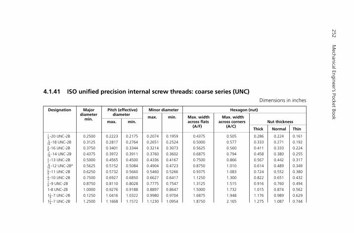
252M
echanical Engineer’s Pocket Book
Dimensions in inches
Designation Major Pitch (effective) Minor diameter Hexagon (nut)diameter diameter
max. min. Max. width Max. width min.max. min. across flats across corners Nut thickness
(A/F) (A/C)Thick Normal Thin
1–4 -20 UNC-2B 0.2500 0.2223 0.2175 0.2074 0.1959 0.4375 0.505 0.286 0.224 0.1615–-16 -18 UNC-2B 0.3125 0.2817 0.2764 0.2651 0.2524 0.5000 0.577 0.333 0.271 0.1923–8 -16 UNC-2B 0.3750 0.3401 0.3344 0.3214 0.3073 0.5625 0.560 0.411 0.333 0.2247–-16 -14 UNC-2B 0.4375 0.3972 0.3911 0.3760 0.3602 0.6875 0.794 0.458 0.380 0.2551–2 -13 UNC-2B 0.5000 0.4565 0.4500 0.4336 0.4167 0.7500 0.866 0.567 0.442 0.3179–-16 -12 UNC-2Ba 0.5625 0.5152 0.5084 0.4904 0.4723 0.8750 1.010 0.614 0.489 0.3495–8 -11 UNC-2B 0.6250 0.5732 0.5660 0.5460 0.5266 0.9375 1.083 0.724 0.552 0.3803–4 -10 UNC-2B 0.7500 0.6927 0.6850 0.6627 0.6417 1.1250 1.300 0.822 0.651 0.4327–8 -9 UNC-2B 0.8750 0.8110 0.8028 0.7775 0.7547 1.3125 1.515 0.916 0.760 0.494
1-8 UNC-2B 1.0000 0.9276 0.9188 0.8897 0.8647 1.5000 1.732 1.015 0.874 0.562
11–8 -7 UNC-2B 0.1250 1.0416 1.0322 0.9980 0.9704 1.6875 1.948 1.176 0.989 0.629
11–4 -7 UNC-2B 1.2500 1.1668 1.1572 1.1230 1.0954 1.8750 2.165 1.275 1.087 0.744
4.1.41 ISO unified precision internal screw threads: coarse series (UNC)
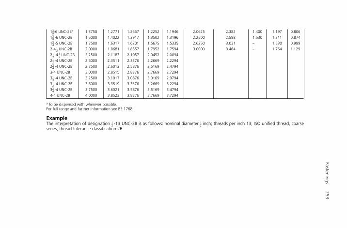
Fastenings253
13–8-6 UNC-2Ba 1.3750 1.2771 1.2667 1.2252 1.1946 2.0625 2.382 1.400 1.197 0.806
13–8 -6 UNC-2B 1.5000 1.4022 1.3917 1.3502 1.3196 2.2500 2.598 1.530 1.311 0.874
13–4 -5 UNC-2B 1.7500 1.6317 1.6201 1.5675 1.5335 2.6250 3.031 – 1.530 0.999
2-41–2 UNC-2B 2.0000 1.8681 1.8557 1.7952 1.7594 3.0000 3.464 – 1.754 1.129
21–4 -41–2 UNC-2B 2.2500 2.1183 2.1057 2.0452 2.0094
21–2 -4 UNC-2B 2.5000 2.3511 2.3376 2.2669 2.2294
23–4 -4 UNC-2B 2.7500 2.6013 2.5876 2.5169 2.4794
3-4 UNC-2B 3.0000 2.8515 2.8376 2.7669 2.7294
31–4 -4 UNC-2B 3.2500 3.1017 3.0876 3.0169 2.9794
31–2 -4 UNC-2B 3.5000 3.3519 3.3376 3.2669 3.2294
33–4 -4 UNC-2B 3.7500 3.6021 3.5876 3.5169 3.4794
4-4 UNC-2B 4.0000 3.8523 3.8376 3.7669 3.7294
a To be dispensed with wherever possible.For full range and further information see BS 1768.
ExampleThe interpretation of designation 1–2 -13 UNC-2B is as follows: nominal diameter 1–2 inch; threads per inch 13; ISO unified thread, coarseseries; thread tolerance classification 2B.
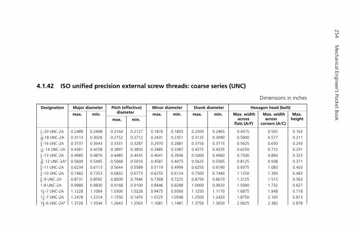
254M
echanical Engineer’s Pocket Book
Dimensions in inches
Designation Major diameter Pitch (effective) Minor diameter Shank diameter Hexagon head (bolt)
max. min. diameter max. min. max. min. Max. width Max. width Max. max. min. across across height
flats (A/F) corners (A/C)
1–4 -20 UNC-2A 0.2489 0.2408 0.2164 0.2127 0.1876 0.1803 0.2500 0.2465 0.4375 0.505 0.1635–-16-18 UNC-2A 0.3113 0.3026 0.2752 0.2712 0.2431 0.2351 0.3125 0.3090 0.5000 0.577 0.2113–4 -16 UNC-2A 0.3737 0.3643 0.3331 0.3287 0.2970 0.2881 0.3750 0.3715 0.5625 0.650 0.2437–-16 -14 UNC-2A 0.4361 0.4258 0.3897 0.3850 0.3485 0.3387 0.4375 0.4335 0.6250 0.722 0.2911–2 -13 UNC-2A 0.4985 0.4876 0.4485 0.4435 0.4041 0.3936 0.5000 0.4960 0.7500 0.866 0.3239–-16 -12 UNC-2Aa 0.5609 0.5495 0.5068 0.5016 0.4587 0.4475 0.5625 0.5585 0.8125 0.938 0.3715–8 -11 UNC-2A 0.6234 0.6113 0.5644 0.5589 0.5119 0.4999 0.6250 0.6190 0.9375 1.083 0.4033–4 -10 UNC-2A 0.7482 0.7353 0.6832 0.6773 0.6255 0.6124 0.7500 0.7440 1.1250 1.300 0.4837–8 -9 UNC-2A 0.8731 0.8592 0.8009 0.7946 0.7368 0.7225 0.8750 0.8670 1.3125 1.515 0.563
1-8 UNC-2A 0.9980 0.9830 0.9168 0.9100 0.8446 0.8288 1.0000 0.9920 1.5000 1.732 0.627
11–8 -7 UNC-2A 1.1228 1.1064 1.0300 1.0228 0.9475 0.9300 1.1250 1.1170 1.6875 1.948 0.718
11–4 -7 UNC-2A 1.2478 1.2314 1.1550 0.1476 1.0725 1.0548 1.2500 1.2420 1.8750 2.165 0.813
13–8 -6 UNC-2Aa 1.3726 1.3544 1.2643 1.2563 1.1681 1.1481 1.3750 1.3650 2.0625 2.382 0.878
4.1.42 ISO unified precision external screw threads: coarse series (UNC)

Fastenings255
11–2 -6 UNC-2A 1.4976 1.4794 1.3893 1.3812 1.2931 1.2730 1.5000 1.4900 2.2500 2.598 0.974
13–4 -5 UNC-2A 1.7473 1.7268 1.6174 1.6085 1.5019 1.4786 1.7500 1.7400 2.6250 3.031 1.134
2-41–2 UNC-2A 1.9971 1.9751 1.8528 1.8433 1.7245 1.6990 2.000 1.9900 3.000 3.464 1.263
21–4 -41–2 UNC-2A 2.2471 2.2251 2.1028 2.0931 1.9745 1.9488
21–2 -4 UNC-2A 2.4969 2.4731 2.3345 2.3241 2.1902 2.1618
23–4 -4 UNC-2A 2.7468 2.7230 2.5844 2.5739 2.4401 2.4116
3-4 UNC-2A 2.9968 2.9730 2.8344 2.8237 2.6901 2.6614
31–4 -4 UNC-2A 3.2467 3.2229 3.0843 3.0734 2.9400 2.9111
31–2 -4 UNC-2A 3.4967 3.4729 3.3343 3.3233 3.1900 3.1610
33–4 -4 UNC-2A 3.7466 3.7228 3.5842 3.5730 3.4399 3.4107
4-4 UNC-2A 3.9966 3.9728 3.8342 3.8229 3.6899 3.6606
a To be dispensed with wherever possible.For full range and further information see BS 1768.
ExampleThe interpretation of designation 1–2 -13 UNC-2A is as follows: nominal diameter 1–2 inch; threads per inch 13; ISO unified thread, coarseseries, thread tolerance classification 2a.
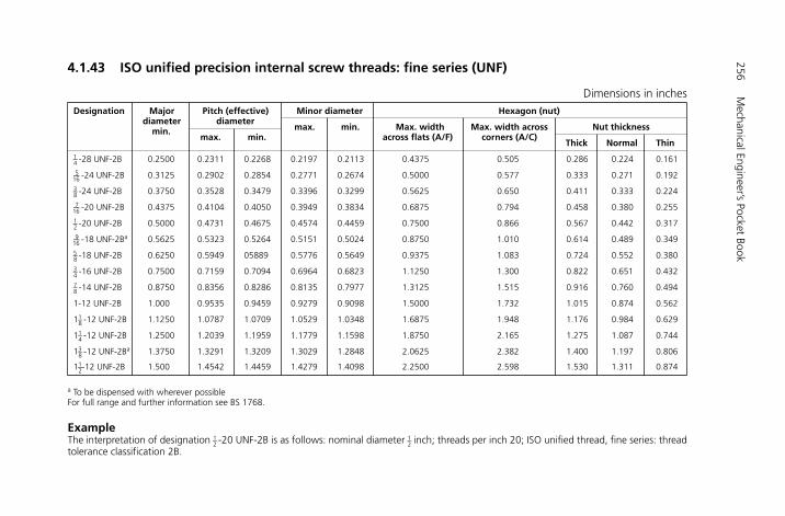
256M
echanical Engineer’s Pocket Book
Dimensions in inchesDesignation Major Pitch (effective) Minor diameter Hexagon (nut)
diameter diametermax. min. Max. width Max. width across Nut thicknessmin.
max. min. across flats (A/F) corners (A/C)Thick Normal Thin
1–4 -28 UNF-2B 0.2500 0.2311 0.2268 0.2197 0.2113 0.4375 0.505 0.286 0.224 0.161
5–-16 -24 UNF-2B 0.3125 0.2902 0.2854 0.2771 0.2674 0.5000 0.577 0.333 0.271 0.192
3–8 -24 UNF-2B 0.3750 0.3528 0.3479 0.3396 0.3299 0.5625 0.650 0.411 0.333 0.224
7–-16 -20 UNF-2B 0.4375 0.4104 0.4050 0.3949 0.3834 0.6875 0.794 0.458 0.380 0.255
1–2 -20 UNF-2B 0.5000 0.4731 0.4675 0.4574 0.4459 0.7500 0.866 0.567 0.442 0.317
9–-16 -18 UNF-2Ba 0.5625 0.5323 0.5264 0.5151 0.5024 0.8750 1.010 0.614 0.489 0.349
5–8 -18 UNF-2B 0.6250 0.5949 05889 0.5776 0.5649 0.9375 1.083 0.724 0.552 0.380
3–4 -16 UNF-2B 0.7500 0.7159 0.7094 0.6964 0.6823 1.1250 1.300 0.822 0.651 0.432
7–8 -14 UNF-2B 0.8750 0.8356 0.8286 0.8135 0.7977 1.3125 1.515 0.916 0.760 0.494
1-12 UNF-2B 1.000 0.9535 0.9459 0.9279 0.9098 1.5000 1.732 1.015 0.874 0.562
11–8 -12 UNF-2B 1.1250 1.0787 1.0709 1.0529 1.0348 1.6875 1.948 1.176 0.984 0.629
11–4 -12 UNF-2B 1.2500 1.2039 1.1959 1.1779 1.1598 1.8750 2.165 1.275 1.087 0.744
13–8 -12 UNF-2Ba 1.3750 1.3291 1.3209 1.3029 1.2848 2.0625 2.382 1.400 1.197 0.806
11–2-12 UNF-2B 1.500 1.4542 1.4459 1.4279 1.4098 2.2500 2.598 1.530 1.311 0.874
a To be dispensed with wherever possibleFor full range and further information see BS 1768.
ExampleThe interpretation of designation 1–2 -20 UNF-2B is as follows: nominal diameter 1–2 inch; threads per inch 20; ISO unified thread, fine series: threadtolerance classification 2B.
4.1.43 ISO unified precision internal screw threads: fine series (UNF)
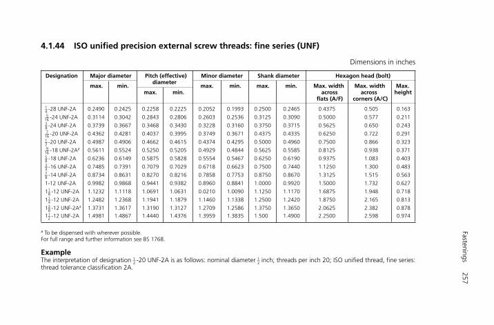
Fastenings257
Dimensions in inches
Designation Major diameter Pitch (effective) Minor diameter Shank diameter Hexagon head (bolt)
max. min.diameter
max. min. max. min. Max. width Max. width Max. max. min. across across height
flats (A/F) corners (A/C)1–4 -28 UNF-2A 0.2490 0.2425 0.2258 0.2225 0.2052 0.1993 0.2500 0.2465 0.4375 0.505 0.1635–-16 -24 UNF-2A 0.3114 0.3042 0.2843 0.2806 0.2603 0.2536 0.3125 0.3090 0.5000 0.577 0.2113–8 -24 UNF-2A 0.3739 0.3667 0.3468 0.3430 0.3228 0.3160 0.3750 0.3715 0.5625 0.650 0.2437–-16 -20 UNF-2A 0.4362 0.4281 0.4037 0.3995 0.3749 0.3671 0.4375 0.4335 0.6250 0.722 0.2911–2 -20 UNF-2A 0.4987 0.4906 0.4662 0.4615 0.4374 0.4295 0.5000 0.4960 0.7500 0.866 0.3239–-16 -18 UNF-2Aa 0.5611 0.5524 0.5250 0.5205 0.4929 0.4844 0.5625 0.5585 0.8125 0.938 0.3715–8 -18 UNF-2A 0.6236 0.6149 0.5875 0.5828 0.5554 0.5467 0.6250 0.6190 0.9375 1.083 0.4033–4 -16 UNF-2A 0.7485 0.7391 0.7079 0.7029 0.6718 0.6623 0.7500 0.7440 1.1250 1.300 0.4837–8 -14 UNF-2A 0.8734 0.8631 0.8270 0.8216 0.7858 0.7753 0.8750 0.8670 1.3125 1.515 0.563
1-12 UNF-2A 0.9982 0.9868 0.9441 0.9382 0.8960 0.8841 1.0000 0.9920 1.5000 1.732 0.627
11–8 -12 UNF-2A 1.1232 1.1118 1.0691 1.0631 0.0210 1.0090 1.1250 1.1170 1.6875 1.948 0.718
11–4 -12 UNF-2A 1.2482 1.2368 1.1941 1.1879 1.1460 1.1338 1.2500 1.2420 1.8750 2.165 0.813
13–8 -12 UNF-2Aa 1.3731 1.3617 1.3190 1.3127 1.2709 1.2586 1.3750 1.3650 2.0625 2.382 0.87811–2 -12 UNF-2A 1.4981 1.4867 1.4440 1.4376 1.3959 1.3835 1.500 1.4900 2.2500 2.598 0.974
a To be dispensed with wherever possible.For full range and further information see BS 1768.
ExampleThe interpretation of designation 1–2 -20 UNF-2A is as follows: nominal diameter 1–2 inch; threads per inch 20; ISO unified thread, fine series:thread tolerance classification 2A.
4.1.44 ISO unified precision external screw threads: fine series (UNF)

258 Mechanical Engineer’s Pocket Book
4.1.45 British Association thread form
British Association (BA) thread forms are obsolete but are still used in repairs and maintenance.
Pitchdiameter
0.268P
1.13
63P
0.268P
Pitch P
0.18P
47 °1–2
H6508-Ch04.1e.qxd 9/12/05 4:41 PM Page 258
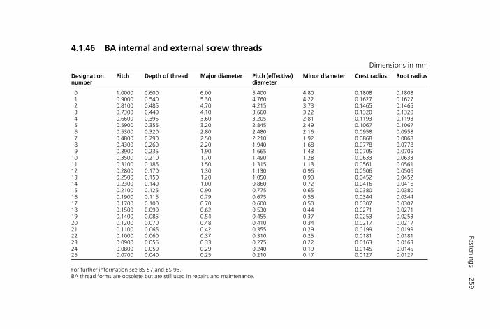
Fastenings259
Dimensions in mmDesignation Pitch Depth of thread Major diameter Pitch (effective) Minor diameter Crest radius Root radiusnumber diameter
0 1.0000 0.600 6.00 5.400 4.80 0.1808 0.18081 0.9000 0.540 5.30 4.760 4.22 0.1627 0.16272 0.8100 0.485 4.70 4.215 3.73 0.1465 0.14653 0.7300 0.440 4.10 3.660 3.22 0.1320 0.13204 0.6600 0.395 3.60 3.205 2.81 0.1193 0.11935 0.5900 0.355 3.20 2.845 2.49 0.1067 0.10676 0.5300 0.320 2.80 2.480 2.16 0.0958 0.09587 0.4800 0.290 2.50 2.210 1.92 0.0868 0.08688 0.4300 0.260 2.20 1.940 1.68 0.0778 0.07789 0.3900 0.235 1.90 1.665 1.43 0.0705 0.0705
10 0.3500 0.210 1.70 1.490 1.28 0.0633 0.063311 0.3100 0.185 1.50 1.315 1.13 0.0561 0.056112 0.2800 0.170 1.30 1.130 0.96 0.0506 0.050613 0.2500 0.150 1.20 1.050 0.90 0.0452 0.045214 0.2300 0.140 1.00 0.860 0.72 0.0416 0.041615 0.2100 0.125 0.90 0.775 0.65 0.0380 0.038016 0.1900 0.115 0.79 0.675 0.56 0.0344 0.034417 0.1700 0.100 0.70 0.600 0.50 0.0307 0.030718 0.1500 0.090 0.62 0.530 0.44 0.0271 0.027119 0.1400 0.085 0.54 0.455 0.37 0.0253 0.025320 0.1200 0.070 0.48 0.410 0.34 0.0217 0.021721 0.1100 0.065 0.42 0.355 0.29 0.0199 0.019922 0.1000 0.060 0.37 0.310 0.25 0.0181 0.018123 0.0900 0.055 0.33 0.275 0.22 0.0163 0.016324 0.0800 0.050 0.29 0.240 0.19 0.0145 0.014525 0.0700 0.040 0.25 0.210 0.17 0.0127 0.0127
For further information see BS 57 and BS 93.BA thread forms are obsolete but are still used in repairs and maintenance.
4.1.46 BA internal and external screw threads
260 Mechanical Engineer’s Pocket Book
4.1.47 BA threads: tapping and clearance drills
4.1.48 ISO metric tapping and clearance drills, coarsethread series
BA no. Tapping size drill Clearance size drill
mm Number or mm Number, letter or fraction size fraction size
0 5.10 8 6.10 D1 4.50 16 5.50 22 4.00 22 4.85 103 3.40 29 4.25 184 3.00 32 3.75 245 2.65 37 3.30 296 2.30 43 2.90 327 2.05 45/46 2.60 368 1.80 50 2.25 419 1.55 53 1.95 45
10 1.40 54 1.75 4911 1.20 56 1.60 5212 1.05 59 1.40 5413 0.98 62 1.30 5514 0.78 68 1.10 5715 0.70 70 0.98 6016 0.60 73 0.88 65
Nominal Tapping drill size (mm) Clearance drill size (mm)size
Recommended Alternative 70% Close Medium Free 80% engagement engagement fit fit fit
M1.6 1.25 1.30 1.7 1.8 2.0M2 1.60 1.65 2.2 2.4 2.6M2.5 2.05 2.10 2.7 2.9 3.1M3 2.50 2.55 3.2 3.4 3.6M4 3.30 3.40 4.3 4.5 4.8M5 4.20 4.30 5.3 5.5 5.8M6 5.00 5.10 6.4 6.6 7.0M8 6.80 6.90 8.4 9.0 10.0M10 8.50 8.60 10.5 11.0 12.0M12 10.20 10.40 13.0 14.0 15.0M14 12.00 12.20 15.0 16.0 17.0M16 14.00 14.25 17.0 18.0 19.0M18 15.50 15.75 19.0 20.0 21.0M20 17.50 17.75 21.0 22.0 24.0M22 19.50 19.75 23.0 24.0 26.0M24 21.00 21.25 25.0 26.0 28.0M27 24.00 24.25 28.0 30.0 32.0M30 26.50 26.75 31.0 33.0 35.0M33 29.50 29.75 34.0 36.0 38.0M36 32.00 – 37.0 39.0 42.0M39 35.00 – 40.0 42.0 45.0M42 37.50 – 43.0 45.0 48.0M45 40.50 – 46.0 48.0 52.0M48 43.00 – 50.0 52.0 56.0M52 47.00 – 54.0 56.0 62.0
H6508-Ch04.1e.qxd 9/12/05 4:41 PM Page 260
Fastenings 261
4.1.49 ISO metric tapping and clearance drills, fine thread series
4.1.50 ISO unified tapping and clearance drills, coarsethread series
Nominal Tapping drill size (mm) Clearance drill size (mm)size
Recommended Alternative 70% Close Medium Free 80% engagement engagement fit fit fit
M6 5.20 5.30 6.4 6.6 7.0M8 7.00 7.10 8.4 9.0 10.0M10 8.80 8.90 10.5 11.0 12.0M12 10.80 10.90 13.0 14.0 15.0M14 12.50 12.70 15.0 16.0 17.0M16 14.50 14.75 17.0 18.0 19.0M18 16.50 16.75 19.0 20.0 21.0M20 18.50 18.75 21.0 22.0 24.0M22 20.50 20.75 23.0 24.0 26.0M24 22.00 22.25 25.0 26.0 28.0M27 25.00 25.25 28.0 30.0 32.0M30 28.00 28.25 31.0 33.0 35.0M33 31.00 31.25 34.0 36.0 38.0M36 33.00 – 37.0 39.0 42.0M39 36.00 – 40.0 42.0 45.0M42 39.00 – 43.0 45.0 48.0
Nominal size Tapping drill size Clearance drill sizein.
mm in. mm Letter or in.1–4 � 20 5.20 13–-64 6.50 F or 17–-645–-16 � 18 6.60 17–-64 8.00 O or 21–-643–4 � 16 8.00 5–-16 9.80 W or 25–-647–-16 � 14 9.40 3–8 11.30 33–-641–2 � 13 10.80 27–-64 13.00 33–-649–-16 � 12 12.20 31–-64 14.75 37–-645–8 � 11 13.50 17–-32 16.25 41–-643–4 � 10 16.50 21–-32 19.50 47–-647–8 � 9 19.25 49–-64 20.25 51–-64
1 � 8 22.25 7–8 25.75 1 1–-64
11–8 � 7 25.00 63–-64 26.00 1 9–-64
11–4 � 7 28.25a 1 7–-64 28.25 117–-64
13–8 � 6 30.50a 113–-64 30.75 125–-64
11–2 � 6 34.00a 121–-64 34.00 133–-64
13–4 � 5 39.50a 135–-64 45.00 149–-64
2 � 41–2 45.50a 125–-64 52.00 2 1–-64
aNearest standard metric size: approximately. 0.25 mm over rec-ommended inch size.
H6508-Ch04.1e.qxd 9/12/05 4:41 PM Page 261
262 Mechanical Engineer’s Pocket Book
4.1.51 ISO unified tapping and clearance drills, fine thread series
Nominal size Tapping drill size Clearance drill sizein.
mm Letter or in. mm Letter or in.1–4 � 28 5.50 7–-32 6.50 F5–-16 � 24 6.90 I 8.00 O3–8 � 24 8.50 R 9.80 W7–-16 � 20 9.90 25–-64 11.30 29–-641–2 � 20 11.50 29–-64 13.00 33–-649–-16 � 18 12.90 33–-64 14.75 37–-645–8 � 18 14.50 37–-64 16.50 41–-643–4 � 16 17.50 11–-16 19.50 49–-647–8 � 14 20.50 13–-16 22.75 57–-64
1 � 12 23.25 59–-64 25.80 1 1–-64
11–8 � 12 26.50 1 3–-64 29.00 1 9–-64
11–4 � 12 29.50 111–-64 32.50 117–-64
13–8 � 12 33.00 119–-64 35.50 125–-64
11–2 � 12 36.00 127–-64 38.50 133–-64
4.1.52 ISO metric tapping and clearance drills, miniature series
Nominal size Pitch Threads Tapping drill size Clearance drill size
ISO ASA B1.10mm per inch
mm Number or mm Number ormm mm fraction fraction
S-0.3 0.30 unm 0.080 318 0.25 – 0.32 –
(S-0.35) (0.35 unm) 0.090 282 0.28 – 0.38 79
S-0.4 0.40 unm 0.100 254 0.35 80 0.45 77
(S-0.45) (0.45 unm) 0.100 254 0.38 79 0.50 76
S-0.5 0.50 unm 0.125 203 0.42 78 0.55 75, 74
(S-0.55) (0.55 unm) 0.125 203 0.45 77 0.60 73
S-0.6 0.60 unm 0.150 169 0.50 76 0.65 72
(S-0.7) (0.70 unm) 0.175 145 0.58 74 0.78 1–-32in.
S-0.8 0.80 unm 0.200 127 0.65 72 0.88 66, 65
(S-0.9) (0.90 unm) 0.225 113 0.72 70 0.98 62
S-1.0 1.00 unm 0.250 102 0.80 1–-32in. 1.10 57
(S-1.1) (1.10 unm) 0.250 102 0.90 65 1.20 3–-64in.
S-1.2 1.20 unm 0.250 102 1.00 61 1.30 55(S-1.4) (1.40 unm) 0.300 85 1.15 3–-64in. 1.50 53
H6508-Ch04.1e.qxd 9/12/05 4:41 PM Page 262
Fastenings 263
4.1.53 BSW threads, tapping and clearance drills
Size TPI Tapping Clearing1–-16 60 58 493–-32 48 49 361–8 40 38 295–-32 32 31 193–-16 24 26 97–-32 24 15 11–4 20 7 G5–-16 18 F P3–8 16 O W7–-16 14 U 29–-641–2 12 27–-64
33–-64
Size T.P.I Tapping Clearing7–-32 28 14 11–4 26 3 G9–-32 26 C M5–-16 22 H P3–8 20 21–-64 W7–-16 18 W 29–-641–2 16 7–-16
33–-64
4.1.54 BSF threads, tapping and clearance drills
4.1.55 Plain washers, bright: metric series
d1
d2 s
H6508-Ch04.1e.qxd 9/12/05 4:41 PM Page 263
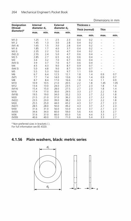
264 Mechanical Engineer’s Pocket Book
4.1.56 Plain washers, black: metric series
d1
d2 ss
Dimensions in mmDesignation Internal External Thickness s(thread diameter d1 diameter d2 Thick (normal) Thindiameter)a
max. min. max. min.max. min. max. min.
M1.0 1.25 1.1 2.5 2.3 0.4 0.2 – –M1.2 1.45 1.3 3.0 2.8 0.4 0.2 – –(M1.4) 1.65 1.5 3.0 2.8 0.4 0.2 – –M1.6 1.85 1.7 4.0 3.7 0.4 0.2 – –M2.0 2.35 2.2 5.0 4.7 0.4 0.2 – –(M2.2) 2.55 2.4 5.0 4.7 0.6 0.4 – –M2.5 2.85 2.7 6.5 6.2 0.6 0.4 – –M3 3.4 3.2 7.0 6.7 0.6 0.4 – –(M3.5) 3.9 3.7 7.0 6.7 0.6 0.4 – –M4 4.5 4.3 9.0 8.7 0.9 0.7 – –(M4.5) 5.0 4.8 9.0 8.7 0.9 0.7 – –M5 5.5 5.3 10.0 9.7 1.1 0.9 – –M6 6.7 6.4 12.5 12.1 1.8 1.4 0.9 0.7(M7) 7.7 7.4 14.0 13.6 1.8 1.4 0.9 0.7M8 8.7 8.4 17.0 16.6 1.8 1.4 1.1 0.9M10 10.9 10.5 21.0 20.5 2.2 1.8 1.45 1.05M12 13.4 13.0 24.0 23.5 2.7 2.3 1.8 1.4(M14) 15.4 15.0 28.0 27.5 2.7 2.3 1.8 1.4M16 17.4 17.0 30.0 29.5 3.3 2.7 2.2 1.8(M18) 19.5 19.0 34.0 33.2 3.3 2.7 2.2 1.8M20 21.5 21.0 37.0 36.2 3.3 2.7 2.2 1.8(M22) 23.5 23.0 39.0 38.2 3.3 2.7 2.2 1.8M24 25.5 25.0 44.0 43.2 4.3 3.7 2.7 2.3(M27) 28.5 28.0 50.0 49.2 4.3 3.7 2.7 2.3M30 31.6 31.0 56.0 55.0 4.3 3.7 2.7 2.3(M33) 34.6 34.0 60.0 59.0 5.6 4.4 3.3 2.7M36 37.6 37.0 66.0 65.0 5.6 4.4 3.3 2.7(M39) 40.6 40.0 72.0 71.0 6.6 5.4 3.3 2.7
a Non-preferred sizes in brackets ( ).For full information see BS 4320.
H6508-Ch04.1e.qxd 9/12/05 4:41 PM Page 264
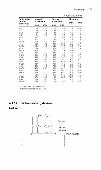
Fastenings 265
4.1.57 Friction locking devices
Lock nut
Lock orjamb nut
Plain washer
Full nut
Dimensions in mmDesignation Internal External Thickness s(thread diameter d1 diameter d2 max. min.diameter)a
max. min. max. min.
M5 5.8 5.5 10.0 9.2 1.2 0.8M6 7.0 6.6 12.5 11.7 1.9 1.3(M7) 8.0 7.6 14.0 13.2 1.9 1.3M8 9.4 9.0 17.0 16.2 1.9 1.3M10 11.5 11.0 21.0 20.2 2.3 1.7M12 14.5 14.0 24.0 23.2 2.8 2.2(M14) 16.5 16.0 28.0 27.2 2.8 2.2M16 18.5 18.0 30.0 29.2 3.6 2.4(M18) 20.6 20.0 34.0 32.8 3.6 2.4M20 22.6 22.0 37.0 35.8 3.6 2.4(M22) 24.6 24.0 39.0 37.8 3.6 2.4M24 26.6 26.0 44.0 42.8 4.6 3.4(M27) 30.6 30.0 50.0 48.8 4.6 3.4M30 33.8 33.0 56.0 54.5 4.6 3.4(M33) 36.8 36.0 60.0 58.5 6.0 4.0M36 39.8 39.0 66.0 64.5 6.0 4.0(M39) 42.8 42.0 72.0 70.5 7.0 5.0M42 45.8 45.0 78.0 76.5 8.2 5.8(M45) 48.8 48.0 85.0 83.0 8.2 5.8M48 53.0 52.0 92.0 90.0 9.2 6.8(M52) 57.0 56.0 98.0 96.0 9.2 6.8M56 63.0 62.0 105.0 103.0 10.2 7.8(M60) 67.0 66.0 110.0 108.0 10.2 7.8M64 71.0 70.0 115.0 113.0 10.2 7.8(M68) 75.0 74.0 120.0 118.0 11.2 8.8
aNon-preferred sizes in brackets ( ).For full information see BS 4320.
H6508-Ch04.1f.qxd 9/12/05 4:44 PM Page 265
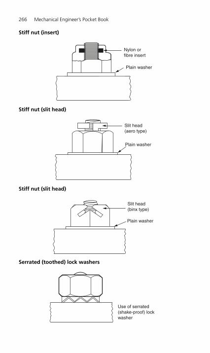
Stiff nut (slit head)
266 Mechanical Engineer’s Pocket Book
Slit head(binx type)
Plain washer
Use of serrated(shake-proof) lockwasher
Serrated (toothed) lock washers
Plain washer
Slit head(aero type)
Stiff nut (slit head)
Plain washer
Nylon orfibre insert
Stiff nut (insert)
H6508-Ch04.1f.qxd 9/12/05 4:44 PM Page 266

Castle nut
Fastenings 267
Split pin
Lock washers, see:Spring washers 4.1.59, 4.1.60, 4.1.61Toothed lock washers 4.1.62Serrated lock washers 4.1.63Crinkle washers 4.1.64
Tab washer
4.1.58 Positive locking devices
Slotted nut
H6508-Ch04.1f.qxd 9/12/05 4:44 PM Page 267
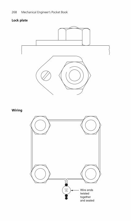
Lock plate
268 Mechanical Engineer’s Pocket Book
Wire endstwistedtogetherand sealed
Wiring
H6508-Ch04.1f.qxd 9/12/05 4:44 PM Page 268
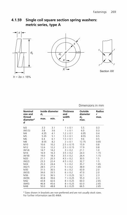
4.1.59 Single coil square section spring washers: metric series, type A
Fastenings 269
s
s
X
X
d2 d1
h � 2s � 15%
r
r
r
r
Section XX
Nominal Inside diameter Thickness Outside Radiussize and d1 and diameter rthread
max. min.width d2 max.
diametera s max.d
M3 3.3 3.1 1 � 0.1 5.5 0.3(M3.5) 3.8 3.6 1 � 0.1 6.0 0.3M4 4.35 4.1 1.2 � 0.1 6.95 0.4M5 5.35 5.1 1.5 � 0.1 8.55 0.5M6 6.4 6.1 1.5 � 0.1 9.6 0.5M8 8.55 8.2 2 � 0.1 12.75 0.65M10 10.6 10.2 2.5 � 0.15 15.9 0.8M12 12.6 12.2 2.5 � 0.15 17.9 0.8(M14) 14.7 14.2 3 � 0.2 21.1 1.0M16 16.9 16.3 3.5 � 0.2 24.3 1.15(M18) 19.0 18.3 3.5 � 0.2 26.4 1.15M20 21.1 20.3 4.5 � 0.2 30.5 1.5(M22) 23.3 22.4 4.5 � 0.2 32.7 1.5M24 25.3 24.4 5 � 0.2 35.7 1.65(M27) 28.5 27.5 5 � 0.2 38.9 1.65M30 31.5 30.5 6 � 0.2 43.9 2.0(M33) 34.6 33.5 6 � 0.2 47.0 2.0M36 37.6 36.5 7 � 0.25 52.1 2.3(M39) 40.8 39.6 7 � 0.25 55.3 2.3M42 43.8 42.6 8 � 0.25 60.3 2.65(M45) 46.8 45.6 8 � 0.25 63.3 2.65M48 50.0 48.8 8 � 0.25 66.5 2.65
a Sizes shown in brackets are non-preferred and are not usually stock sizes.For further information see BS 4464.
Dimensions in mm
H6508-Ch04.1f.qxd 9/12/05 4:44 PM Page 269
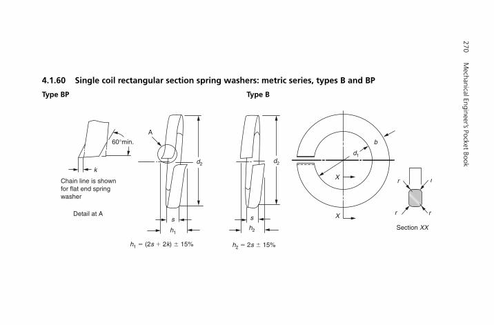
4.1.60 Single coil rectangular section spring washers: metric series, types B and BP
Type BP Type B
270M
echanical Engineer’s Pocket Book
60°min.
Chain line is shownfor flat end springwasher
Detail at A
A
d2 d2
d1
X
X
Section XX
b
r r
rr
h1h2
h1 � (2s � 2k) � 15% h2 � 2s � 15%
s s
k
Fastenings271
Nominal size and Inside diameter d1 Width Thickness Outside diameter Radius r k (type BP only)thread diametera d
max. min.b s d2 max. max.
M1.6 1.9 1.7 0.7 � 0.1 0.4 � 0.1 3.5 0.15 –M2 2.3 2.1 0.9 � 0.1 0.5 � 0.1 4.3 0.15 –(M2.2) 2.5 2.3 1.0 � 0.1 0.6 � 0.1 4.7 0.2 –M2.5 2.8 2.6 1.0 � 0.1 0.6 � 0.1 5.0 0.2 –M3 3.3 3.1 1.3 � 0.1 0.8 � 0.1 6.1 0.25 –(M3.5) 3.8 3.6 1.3 � 0.1 0.8 � 0.1 6.6 0.25 0.15M4 4.35 4.1 1.5 � 0.1 0.9 � 0.1 7.55 0.3 0.15M5 5.35 5.1 1.8 � 0.1 1.2 � 0.1 9.15 0.4 0.15M6 6.4 6.1 2.5 � 0.15 1.6 � 0.1 11.7 0.5 0.2M8 8.55 8.2 3 � 0.15 2 � 0.1 14.85 0.65 0.3M10 10.6 10.2 3.5 � 0.2 2.2 � 0.15 18.0 0.7 0.3M12 12.6 12.2 4 � 0.2 2.5 � 0.15 21.0 0.8 0.4(M14) 14.7 14.2 4.5 � 0.2 3 � 0.15 24.1 1.0 0.4M16 16.9 16.3 5 � 0.2 3.5 � 0.2 27.3 1.15 0.4(M18) 19.0 18.3 5 � 0.2 3.5 � 0.2 29.4 1.15 0.4M20 21.1 20.3 6 � 0.2 4 � 0.2 33.5 1.3 0.4(M22) 23.3 22.4 6 � 0.2 4 � 0.2 35.7 1.3 0.4M24 25.3 24.4 7 � 0.25 5 � 0.2 39.8 1.65 0.5(M27) 28.5 27.5 7 � 0.25 5 � 0.2 43.0 1.65 0.5M30 31.5 30.5 8 � 0.25 6 � 0.25 48.0 2.0 0.8(M33) 34.6 33.5 10 � 0.25 6 � 0.25 55.1 2.0 0.8M36 37.6 36.5 10 � 0.25 6 � 0.25 58.1 2.0 0.8(M39) 40.8 39.6 10 � 0.25 6 � 0.25 61.3 2.0 0.8M42 43.8 42.6 12 � 0.25 7 � 0.25 68.3 2.3 0.8(M45) 46.8 45.6 12 � 0.25 7 � 0.25 71.3 2.3 0.8M48 50.0 48.8 12 � 0.25 7 � 0.25 74.5 2.3 0.8(M52) 54.1 52.8 14 � 0.25 8 � 0.25 82.6 2.65 1.0M56 58.1 56.8 14 � 0.25 8 � 0.25 86.6 2.65 1.0(M60) 62.3 60.9 14 � 0.25 8 � 0.25 90.8 2.65 1.0M64 66.3 64.9 14 � 0.25 8 � 0.25 93.8 2.65 1.0(M68) 70.5 69.0 14 � 0.25 8 � 0.25 99.0 2.65 1.0
a Sizes shown in brackets are non-preferred, and are not usually stock sizes.For further information see BS 4464.
Dimensions in mm
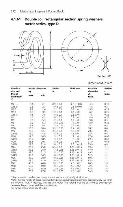
4.1.61 Double coil rectangular section spring washers:metric series, type D
272 Mechanical Engineer’s Pocket Book
r r
rr
d2 d1
h ≈ 5s
s
b
b
x
x
Section XX
Nominal Inside diameter Width Thickness Outside Radiussize and d1 b s diameter rthread
max. min.d2 max.
diametera max.d
M2 2.4 2.1 0.9 � 0.1 0.5 � 0.05 4.4 0.15(M2.2) 2.6 2.3 1.0 � 0.1 0.6 � 0.05 4.8 0.2M2.5 2.9 2.6 1.2 � 0.1 0.7 � 0.1 5.5 0.23M3.0 3.6 3.3 1.2 � 0.1 0.8 � 0.1 6.2 0.25(M3.5) 4.1 3.8 1.6 � 0.1 0.8 � 0.1 7.5 0.25M4 4.6 4.3 1.6 � 0.1 0.8 � 0.1 8.0 0.25M5 5.6 5.3 2 � 0.1 0.9 � 0.1 9.8 0.3M6 6.6 6.3 3 � 0.15 1 � 0.1 12.9 0.33M8 8.8 8.4 3 � 0.15 1.2 � 0.1 15.1 0.4M10 10.8 10.4 3.5 � 0.20 1.2 � 0.1 18.2 0.4M12 12.8 12.4 3.5 � 0.2 1.6 � 0.1 20.2 0.5(M14) 15.0 14.5 5 � 0.2 1.6 � 0.1 25.4 0.5M16 17.0 16.5 5 � 0.2 2 � 0.1 27.4 0.65(M18) 19.0 18.5 5 � 0.2 2 � 0.1 29.4 0.65M20 21.5 20.8 5 � 0.2 2 � 0.1 31.9 0.65(M22) 23.5 22.8 6 � 0.2 2.5 � 0.15 35.9 0.8M24 26.0 25.0 6.5 � 0.2 3.25 � 0.15 39.4 1.1(M27) 29.5 28.0 7 � 0.25 3.25 � 0.15 44.0 1.1M30 33.0 31.5 8 � 0.25 3.25 � 0.15 49.5 1.1(M33) 36.0 34.5 8 � 0.25 3.25 � 0.15 52.5 1.1M36 40.0 38.0 10 � 0.25 3.25 � 0.15 60.5 1.1(M39) 43.0 41.0 10 � 0.25 3.25 � 0.15 63.5 1.1M42 46.0 44.0 10 � 0.25 4.5 � 0.2 66.5 1.5M48 52.0 50.0 10 � 0.25 4.5 � 0.2 72.5 1.5M56 60.0 58.0 12 � 0.25 4.5 � 0.2 84.5 1.5M64 70.0 67.0 12 � 0.25 4.5 � 0.2 94.5 1.5
a Sizes shown in brackets are non-preferred, and are not usually stock sizes.Note: The free height of double coil washers before compression is normally approximately five timesthe thickness but, if required, washers with other free heights may be obtained by arrangementbetween the purchaser and the manufacturer.For further information see BS 4464.
Dimensions in mm
H6508-Ch04.1f.qxd 9/12/05 4:44 PM Page 272

4.1.62 Toothed lock washers, metric
Type A externally toothed
Fastenings 273
d2
s1
d1
min. 2s1
d2s1
d1
min. 2s1
Type J internally toothed
H6508-Ch04.1f.qxd 9/12/05 4:44 PM Page 273

274 Mechanical Engineer’s Pocket Book
Details left unspecified are to be designed as appropriate.
Designation of a toothed lock washer type J with hole diameter d1 � 6.4 mm of springsteel, surface phosphated for protection against rusting (phr): toothed lock washer J 6.4DIN 6797 – phr.
If toothed lock washers are required for left hand threaded bolts, the designation reads:toothed lock washer J 6.4 left DIN 6797 – phr.
Type V countersunk
s2
d1
d3
90°
H6508-Ch04.1f.qxd 9/12/05 4:44 PM Page 274
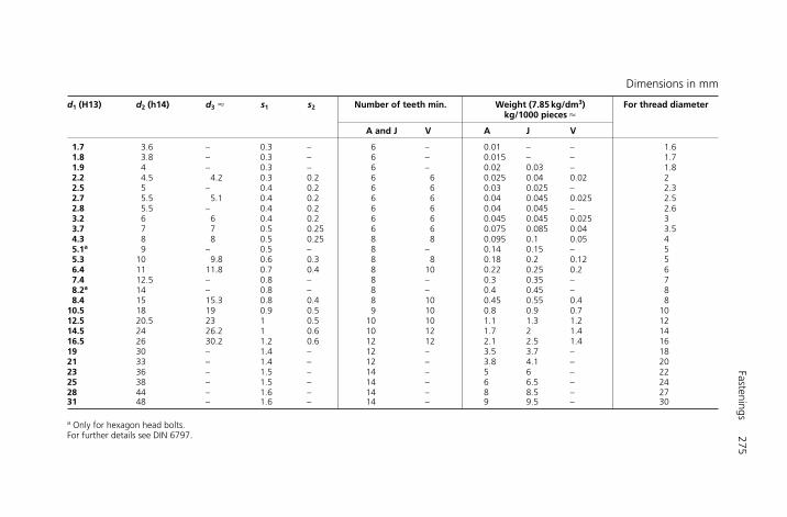
Fastenings275
d1 (H13) d2 (h14) d3 � s1 s2 Number of teeth min. Weight (7.85 kg/dm3) For thread diameterkg/1000 pieces �
A and J V A J V
1.7 3.6 – 0.3 – 6 – 0.01 – – 1.61.8 3.8 – 0.3 – 6 – 0.015 – – 1.71.9 4 – 0.3 – 6 – 0.02 0.03 – 1.82.2 4.5 4.2 0.3 0.2 6 6 0.025 0.04 0.02 22.5 5 – 0.4 0.2 6 6 0.03 0.025 – 2.32.7 5.5 5.1 0.4 0.2 6 6 0.04 0.045 0.025 2.52.8 5.5 – 0.4 0.2 6 6 0.04 0.045 – 2.63.2 6 6 0.4 0.2 6 6 0.045 0.045 0.025 33.7 7 7 0.5 0.25 6 6 0.075 0.085 0.04 3.54.3 8 8 0.5 0.25 8 8 0.095 0.1 0.05 45.1a 9 – 0.5 – 8 – 0.14 0.15 – 55.3 10 9.8 0.6 0.3 8 8 0.18 0.2 0.12 56.4 11 11.8 0.7 0.4 8 10 0.22 0.25 0.2 67.4 12.5 – 0.8 – 8 – 0.3 0.35 – 78.2a 14 – 0.8 – 8 – 0.4 0.45 – 88.4 15 15.3 0.8 0.4 8 10 0.45 0.55 0.4 8
10.5 18 19 0.9 0.5 9 10 0.8 0.9 0.7 1012.5 20.5 23 1 0.5 10 10 1.1 1.3 1.2 1214.5 24 26.2 1 0.6 10 12 1.7 2 1.4 1416.5 26 30.2 1.2 0.6 12 12 2.1 2.5 1.4 1619 30 – 1.4 – 12 – 3.5 3.7 – 1821 33 – 1.4 – 12 – 3.8 4.1 – 2023 36 – 1.5 – 14 – 5 6 – 2225 38 – 1.5 – 14 – 6 6.5 – 2428 44 – 1.6 – 14 – 8 8.5 – 2731 48 – 1.6 – 14 – 9 9.5 – 30
a Only for hexagon head bolts.For further details see DIN 6797.
Dimensions in mm
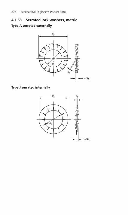
4.1.63 Serrated lock washers, metric
Type A serrated externally
276 Mechanical Engineer’s Pocket Book
�3s1
s1
d1
d2
�3s1
s1d2
d1
Type J serrated internally
H6508-Ch04.1f.qxd 9/12/05 4:45 PM Page 276

Details left unspecified are to be designed as appropriate.
Designation of a serrated lock washer type J with hole diameter d1 � 6.4 mm in springsteel, surface phosphated for protection against rusting (phr): serrated lock washer J 6.4DIN 6798 – phr.
If serrated lock washers are required for left hand threaded bolts, the designation reads:serrated lock washer J 6.4 left DIN 6798 – phr.
Fastenings 277
d1
s2
d3
90°
Type V countersunk
H6508-Ch04.1f.qxd 9/12/05 4:45 PM Page 277
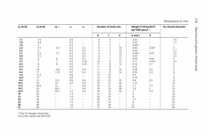
d1 (H13) d2 (h14) d3 � s1 s2 Number of teeth min. Weight (7.85 kg/dm3) For thread diameterkg/1000 pieces �
A J V A and J V
1.7 3.6 0.3 – 9 7 – 0.02 – 1.61.8 3.8 0.3 – 9 7 – 0.02 – 1.71.9 4 0.3 – 9 7 – 0.025 – –2.2 4.5 4.2 0.3 0.2 9 7 10 0.03 0.025 22.5 5 0.4 0.2 9 7 10 0.04 – 2.32.7 5.5 5.1 0.4 0.2 9 7 10 0.045 0.03 2.52.8 5.5 0.4 0.2 9 7 10 0.05 – 2.63.2 6 6 0.4 0.2 9 7 12 0.06 0.04 33.7 7 7 0.5 0.25 10 8 12 0.11 0.075 3.54.3 8 8 0.5 0.25 11 8 14 0.14 0.1 45.1a 9 0.5 – 11 8 – 0.22 – 55.3 10 9.8 0.6 0.3 11 8 14 0.28 0.2 56.4 11 11.8 0.7 0.4 12 9 16 0.36 0.3 67.4 12.5 0.8 – 14 10 – 0.5 – 78.2a 14 0.8 – 14 10 – 0.75 – 88.4 15 15.3 0.8 0.4 14 10 18 0.8 0.5 8
10.5 18 19 0.9 0.5 16 12 20 1.25 1 1012.5 20.5 23 1 0.5 16 12 26 1.7 1.5 1214.5 24 26.2 1 0.6 18 14 28 2.4 2 1416.5 26 30.2 1.2 0.6 18 14 30 3 2.4 1619 30 – 1.4 – 18 14 – 5 – 1821 33 – 1.4 – 20 16 – 6 – 2023 36 – 1.5 – 20 16 – 7.5 – 2225 38 – 1.5 – 20 16 – 8 – 2428 44 – 1.6 – 22 18 – 12 – 2731 48 – 1.6 – 22 18 – 14 – 30
a Only for hexagon head bolts.For further details see DIN 6797.
278M
echanical Engineer’s Pocket Book
Dimensions in mm
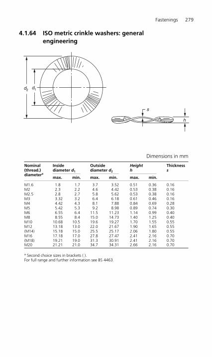
4.1.64 ISO metric crinkle washers: generalengineering
Fastenings 279
d2 d1
h
s
Nominal Inside Outside Height Thickness (thread.) diameter d1 diameter d2 h sdiametera
max. min. max. min. max. min.
M1.6 1.8 1.7 3.7 3.52 0.51 0.36 0.16M2 2.3 2.2 4.6 4.42 0.53 0.38 0.16M2.5 2.8 2.7 5.8 5.62 0.53 0.38 0.16M3 3.32 3.2 6.4 6.18 0.61 0.46 0.16M4 4.42 4.3 8.1 7.88 0.84 0.69 0.28M5 5.42 5.3 9.2 8.98 0.89 0.74 0.30M6 6.55 6.4 11.5 11.23 1.14 0.99 0.40M8 8.55 8.4 15.0 14.73 1.40 1.25 0.40M10 10.68 10.5 19.6 19.27 1.70 1.55 0.55M12 13.18 13.0 22.0 21.67 1.90 1.65 0.55(M14) 15.18 15.0 25.5 25.17 2.06 1.80 0.55M16 17.18 17.0 27.8 27.47 2.41 2.16 0.70(M18) 19.21 19.0 31.3 30.91 2.41 2.16 0.70M20 21.21 21.0 34.7 34.31 2.66 2.16 0.70
a Second choice sizes in brackets ( ).For full range and further information see BS 4463.
Dimensions in mm
H6508-Ch04.1f.qxd 9/12/05 4:45 PM Page 279

4.1.65 T-slot profiles
280M
echanical Engineer’s Pocket Book
Remove sharp corner.0.3 � 45° max.
F
G
KA1
B1
C1
H
P

Fastenings281
Width of throat A1 Width of Depth of Overall Chamfer � 45° Pitch P (avoid pitch
Ordinary For use asrecess recess depth of or radius values in brackets
(H12) tenon (HB)B1 c1 T-slot H
K F Gas they lead to
min. max. min. max. min. max. max. max. max.weakness)
M4 5 �0.12 �0.018 10 11 3.5 4.5 8 10 20 25 32M5 6 0 0 11 12.5 5 6 11 13 25 32 40M6 8 �0.15 �0.022 14.5 16 7 8 15 18 1.0 1.0 32 40 50M8 10 0 0 16 18 7 8 17 21 0.6 40 50 63M10 12 �0.18 �0.027 19 21 8 9 20 25 (40) 50 63 80M12 14 0 0 23 25 9 11 23 28 (50) 63 80 100M16 18 30 32 12 14 30 36
1.61.6 (63) 80 100 125
M20 22 �0.21 �0.033 37 40 16 18 38 45 1.0 (80) 100 125 160M24 28 0 46 50 20 22 48 56 2.5 100 125 160 200M30 36 �0.25 �0.039 56 60 25 28 61 71 125 160 200 250M36 42 0 0 68 72 32 35 74 85
2.51.6 4.0 160 200 250 320
M42 48 80 85 36 40 84 95 200 250 320 400M48 54 �0.30 �0.046 90 95 40 44 94 106 2.0 6.0 250 320 400 500
0 0
Des
ign
atio
ns
of
T-sl
ot
No
min
al
Dimensions in mm
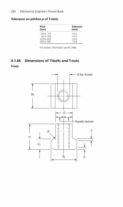
Tolerance on pitches p of T-slots
282 Mechanical Engineer’s Pocket Book
Pitch Tolerance(mm) (mm)
20 to 25 �0.232 to 100 �0.3
125 to 250 �0.5320 to 500 �0.8
For further information see BS 2485.
4.1.66 Dimensions of T-bolts and T-nuts
T-nut
K dia. thread
Equally spaced
B2
B2
G
R F
E
H
C2
H6508-Ch04.1f.qxd 9/12/05 4:45 PM Page 282
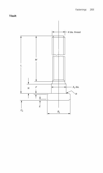
T-bolt
Fastenings 283
K dia. thread
A2 dia.F
R
M
L
E
B2C2
N
H6508-Ch04.1f.qxd 9/12/05 4:45 PM Page 283
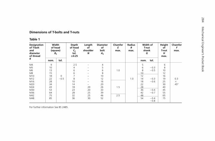
Dimensions of T-bolts and T-nuts
284M
echanical Engineer’s Pocket Book
Table 1
Designation Width Depth Length Diameter Chamfer Radius Width of Height Chamfer of T-bolt of head of head of of E R T-nut of Fand (square) C2 shoulder bolt max. max. shank T-nut max.diameter B2 tol. N A2 G Hof thread �0.25 max.K
nom. tol. nom. tol.
M4 9 2.5 – 4 5 6M5 10 4 – 5 6 �0.3 8M6 13 6 – 6 1.0 8 �0.5 10M8 15 6 – 8 10 12M10 18 0 7 – 10 12 16M12 22 �0.5 8 – 12 1.0 14 �0.3 19 0.3M16 28 10 – 16 18 �0.6 25 �M20 34 14 – 20 22 30 45°M24 43 18 20 26 1.5 28 40M30 53 23 20 33 36 �0.4 45M36 64 28 25 39 42 �0.7 55M42 75 32 25 46 2.5 48 65M48 85 36 30 52 54 �0.4 75
�0.8
For further information See BS 2485.
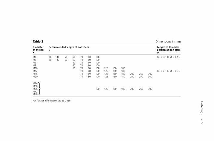
Fastenings285
Table 2 Dimensions in mm
Diameter Recommended length of bolt stem Length of threaded of thread L portion of bolt stemK M
M4 30 40 50 60 70 80 100 For L � 100 M � 0.5 LM5 30 40 50 60 70 80 100M6 60 70 80 100M8 60 70 80 100M10 60 70 80 100 125 160 180M12 70 80 100 125 160 180 For L � 100 M � 0.3 LM16 70 80 100 125 160 180 200 250 300M20 70 80 100 125 160 180 200 250 300
M24M30M36 � 100 125 160 180 200 250 300M42M48
For further information see BS 2485.

4.1.67 Dimensions of tenons for T-slots
286 Mechanical Engineer’s Pocket Book
R
E
D
E
B dia.
A dia.
W
B2
Q
P
L
H6508-Ch04.1f.qxd 9/12/05 4:45 PM Page 286
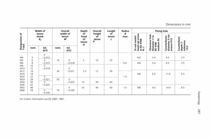
Width of Overall Depth Overall Length Radius Fixing holetenon width of of height of Rshank tenon head of tenon max.
B2 W of tenon Ltenon
nom. tol. nom. tol. Q
P
(h7) (h7)
0M4 5 �0.012 M2 2.4 4.3 2.5M5 6 0 16 0 5 10 25M6 8 �0.015 �0.018 0.6 M3 3.4 6.0 3.5M8 10 0M10 12 �0.018 0M12 14 30 �0.021 5.5 12 30M16 18 M6 6.6 11.0 6.5M20 22 0 1.0M24 28 �0.021 50 0M30 36 0 �0.025 15 30 40M36 42 �0.025M42 48 0 25 40 60 1.5 M8 9.0 14.0 8.5M48 54 0 70 �0.030
�0.030
For further information see BS 2485: 1987.
Fastenings287
Des
ign
atio
n o
fT-
slo
t
To s
uit
so
cket
hea
d c
ap s
crew
to B
S41
68:
Pt1
Cle
aran
ce h
ole
dia
met
erA
toB
S41
86m
ediu
m f
it
Co
un
terb
ore
sd
iam
eter
Bto
l-er
ance
H13
Co
un
terb
ore
dep
th D
tole
ran
ce�
0.2
Dimensions in mm
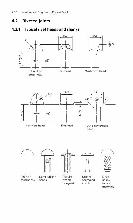
288 Mechanical Engineer’s Pocket Book
4.2 Riveted joints
4.2.1 Typical rivet heads and shanks
2D 2D
Round orsnap head
Leng
th
Pan head Mushroom head
60°D
D
fD
32
2D2D 2D
Leng
th
90°
90° countersunkhead
DfD 4
Flat headConoidal head
Plain orsolid shank
Semi-tubularshank
Tubularshankor eyelet
Split orbifurcatedshank
Driveshankfor softmaterials
H6508-Ch04.2.qxd 9/12/05 4:46 PM Page 288

4.2.2 Typical riveted lap joints
Single row lap joint
Double row (chain) lap joint
Double row (zigzag) lap joint
3D 3D
3D
Lap
6D
Pitc
h
Pitch
1.5D
3D1.5D 3D 3D
3D1.5D
1.5D
Lap
6D
3D 3D
Pitch
3D Pitc
hD � rivet shank diameter3D1.5D
1.5DLa
p 3D
3D 3D
Pitch
Fastenings 289
H6508-Ch04.2.qxd 9/12/05 4:46 PM Page 289

4.2.3 Typical riveted butt joints
Single strap chain riveted butt joint (single row)
Note: This joint may also be double row riveted, chain or zigzag. The strap width � 12Dwhen double riveted (pitch between rows � 3D).
Double strap chain riveted butt joint (double row)
Note: This joint may also be double row zigzag riveted (see Section 4.2.2) or it may be single riveted as above.
1.5D 3D 3D 3D
1.5D
3D1.
5D1.
5D3D
Pitch
Pitc
hP
itch
Str
ap o
r co
ver
plat
e w
idth
= 1
2D
Pitch
Strap orcover plate
1.5D
1.5D
Str
ip w
idth
� 6
D
1.5D
1.5D 3D D � Rivet shank diameter3D3D
290 Mechanical Engineer’s Pocket Book
H6508-Ch04.2.qxd 9/12/05 4:46 PM Page 290
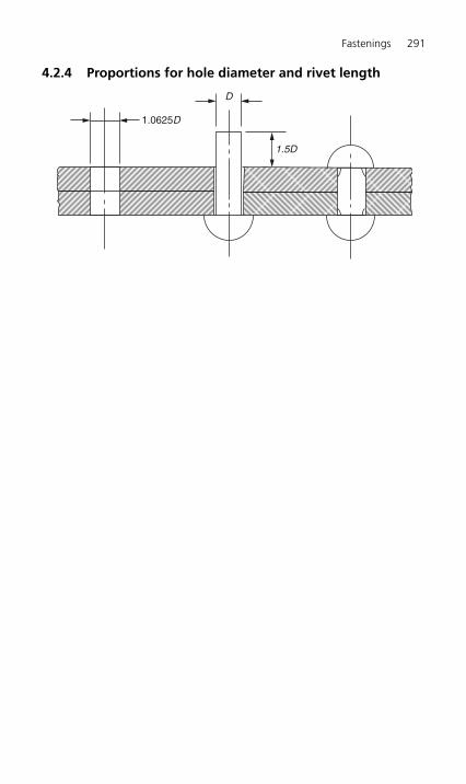
Fastenings 291
4.2.4 Proportions for hole diameter and rivet length
1.0625D
D
1.5D
H6508-Ch04.2.qxd 9/12/05 4:46 PM Page 291

292 Mechanical Engineer’s Pocket Book
Dimensions in mm
Nominal Tolerance Nominal Tolerance Nominal Tolerance Toleranceshank on head on head on head on
diametera diameter diameter diameter depth depth lengthd d D D K K L
1 1.8 0.6 �0.21.2 2.1 �0.2 0.7 �0.01.6 �0.07 2.8 1.02.0 3.5 �0.24 1.2 �0.242.5 4.4 1.5 �0.03.0 5.3 1.8 �0.5
�0.0(3.5) 6.1 �0.29 2.1 �0.294 �0.09 7.0 2.4 �0.05 8.8 3.06 10.5 3.6
�0.35�0.35 �0.0
(7) 12.3 4.2 �0.88 �0.11 14.0 4.8 �0.0
10 18.0 6.012 21.0 �0.42 7.2 �0.42 �1.0(14) �0.14 25.0 8.4 �0.0 �0.016 28.0 9.6
aRivet sizes shown in brackets are non-preferred.For further information see BS 4620: 1970.
4.2.5 Cold forged snap head rivets
d
L
K
D
With d � 16 mm or smallerD � 1.75dK � 0.6dL � length
H6508-Ch04.2.qxd 9/12/05 4:46 PM Page 292
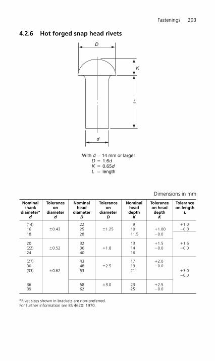
Fastenings 293
Dimensions in mm
Nominal Tolerance Nominal Tolerance Nominal Tolerance Toleranceshank on head on head on head on length
diametera diameter diameter diameter depth depth Ld d D D K K
(14) 22 9 �1.016 �0.43 25 �1.25 10 �1.00 �0.018 28 11.5 �0.0
20 32 13 �1.5 �1.6(22) �0.52 36 �1.8 14 �0.0 �0.024 40 16
(27) 43 17 �2.030 48 �2.5 19 �0.0(33) �0.62 53 21 �3.0
�0.0
36 58 �3.0 23 �2.539 62 25 �0.0
aRivet sizes shown in brackets are non-preferred.For further information see BS 4620: 1970.
4.2.6 Hot forged snap head rivets
D
L
K
d
With d � 14 mm or larger D � 1.6d K � 0.65d L � length
H6508-Ch04.2.qxd 9/12/05 4:46 PM Page 293

294M
echanical Engineer’s Pocket Book
Dimensions in mm
Nominal Nominal length* Lshank
3 4 5 6 8 10 12 14 16 (18) 20 (22) 25 (28) 30 (32) 35 (38) 40 45 50 55diametera d
1.0 � � � � � � � � � �1.2 � � � � � � � � � �1.6 � � � � � � � � � � � �2.0 � � � � � � � � � � � �2.5 � � � � � � � � � � � �3.0 � � � � � � � � � � � �(3.5)4.0 � � � � � � � � �5.0 � � � � � � � � � � � � � �6.0 � � � � � � � � � � � � � � �
aSizes and lengths shown in brackets are non-preferred and should be avoided if possible. The inclusion of dimensional data is not intended to imply that all the productsdescribed are stock production sizes. The purchaser should consult the manufacturer concerning lists of stock production sizes.For the full range of head types and sizes up to and including 39 mm diameter by 160 mm shank length see BS 4620: 1970.
4.2.7 Tentative range of nominal lengths associated with shank diameters
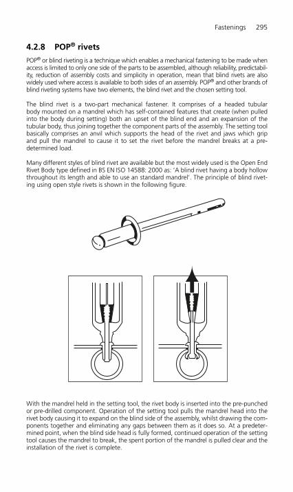
Fastenings 295
4.2.8 POP® rivets
POP® or blind riveting is a technique which enables a mechanical fastening to be made whenaccess is limited to only one side of the parts to be assembled, although reliability, predictabil-ity, reduction of assembly costs and simplicity in operation, mean that blind rivets are alsowidely used where access is available to both sides of an assembly. POP® and other brands ofblind riveting systems have two elements, the blind rivet and the chosen setting tool.
The blind rivet is a two-part mechanical fastener. It comprises of a headed tubular body mounted on a mandrel which has self-contained features that create (when pulledinto the body during setting) both an upset of the blind end and an expansion of thetubular body, thus joining together the component parts of the assembly. The setting toolbasically comprises an anvil which supports the head of the rivet and jaws which grip and pull the mandrel to cause it to set the rivet before the mandrel breaks at a pre-determined load.
Many different styles of blind rivet are available but the most widely used is the Open EndRivet Body type defined in BS EN ISO 14588: 2000 as: ‘A blind rivet having a body hollowthroughout its length and able to use an standard mandrel’. The principle of blind rivet-ing using open style rivets is shown in the following figure.
With the mandrel held in the setting tool, the rivet body is inserted into the pre-punchedor pre-drilled component. Operation of the setting tool pulls the mandrel head into therivet body causing it to expand on the blind side of the assembly, whilst drawing the com-ponents together and eliminating any gaps between them as it does so. At a predeter-mined point, when the blind side head is fully formed, continued operation of the settingtool causes the mandrel to break, the spent portion of the mandrel is pulled clear and theinstallation of the rivet is complete.
H6508-Ch04.2.qxd 9/12/05 4:46 PM Page 295
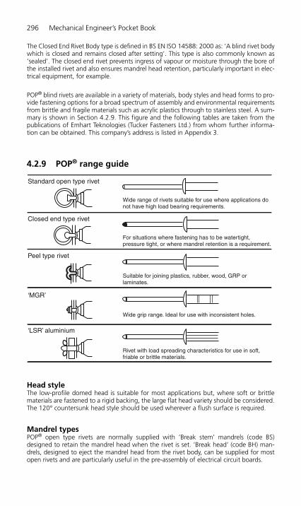
The Closed End Rivet Body type is defined in BS EN ISO 14588: 2000 as: ‘A blind rivet bodywhich is closed and remains closed after setting’. This type is also commonly known as‘sealed’. The closed end rivet prevents ingress of vapour or moisture through the bore ofthe installed rivet and also ensures mandrel head retention, particularly important in elec-trical equipment, for example.
POP® blind rivets are available in a variety of materials, body styles and head forms to pro-vide fastening options for a broad spectrum of assembly and environmental requirementsfrom brittle and fragile materials such as acrylic plastics through to stainless steel. A sum-mary is shown in Section 4.2.9. This figure and the following tables are taken from thepublications of Emhart Teknologies (Tucker Fasteners Ltd.) from whom further informa-tion can be obtained. This company’s address is listed in Appendix 3.
4.2.9 POP® range guide
Head styleThe low-profile domed head is suitable for most applications but, where soft or brittlematerials are fastened to a rigid backing, the large flat head variety should be considered.The 120° countersunk head style should be used wherever a flush surface is required.
Mandrel typesPOP® open type rivets are normally supplied with ‘Break stem’ mandrels (code BS)designed to retain the mandrel head when the rivet is set. ‘Break head’ (code BH) man-drels, designed to eject the mandrel head from the rivet body, can be supplied for mostopen rivets and are particularly useful in the pre-assembly of electrical circuit boards.
Standard open type rivet
Closed end type rivet
Peel type rivet
‘MGR’
‘LSR’ aluminium
Wide range of rivets suitable for use where applications donot have high load bearing requirements.
For situations where fastening has to be watertight,pressure tight, or where mandrel retention is a requirement.
Suitable for joining plastics, rubber, wood, GRP or laminates.
Wide grip range. Ideal for use with inconsistent holes.
Rivet with load spreading characteristics for use in soft,friable or brittle materials.
296 Mechanical Engineer’s Pocket Book
H6508-Ch04.2.qxd 9/12/05 4:46 PM Page 296
Fastenings 297
Finish● Rivet body standard finishes: Steel and nickel-copper rivet bodies are normally supplied
zinc plated.● Paint and other finishes: Rivets with differing surface finishes and paint colours can be
provided on request. Aluminium alloy rivets are available anodized and dyed, matt orgloss for aesthetic and environmental reasons.
4.2.10 Good fastening practice
Blind riveting is a highly reliable and proven method of fixing material together perman-ently. To achieve a superior fastening, the following principles should be considered.
Workpiece materialsWhen materials of different thickness or strengths are being joined, the stronger material –if possible – should be on the blind side. For example, if plastic and metal are to be joined,the plastic sheet should be beneath the rivet head and the metal component should beon the blind side.
Hole size and preparationAchieving a good joint depends on good hole preparation, preferably punched and, ifnecessary, de-burred to the sizes recommended in the POP® blind rivet data tables.
Rivet diameterAs a guide for load-bearing joints, the rivet diameter should be at least equal to the thick-ness of the thickest sheet and not more than three times the thickness of the sheet imme-diately under the rivet head. Refer to data tables for rivet strength characteristics.
Edge distanceRivet holes should be drilled or punched at least two diameters away from an edge – butno more than 24 diameters from that edge.
Rivet pitchAs a guide to the distance between the rivets in load-carrying joint situations, this dis-tance should never exceed three rivet diameters. In butt construction it is advisable toinclude a reinforcing cover strip, fastening it to the underlying sheet by staggered rivets.
Rivet materialChoosing rivets of the correct material normally depends on the strength needed in theriveted joint. When this leads to rivets of material different to the sheets being joined it isimportant to be aware that electrolytic action may cause corrosion. (See Section 4.2.12.)
Setting and safetyThe type of setting tool is usually selected to suit the production environment. The toolmust be cleared of spent materials before setting the next rivet and, in the case of poweroperated tools, must not be operated without the mandrel deflector or mandrel collec-tion system being in position. Safety glasses or goggles should always be worn.
4.2.11 Selection of POP® (or blind) rivets
Joint strengthFirst assess the tensile strength and the shear-load strength required by the joint, both ofwhich can be achieved by the correct number and spacing of fastenings, and by choosinga rivet with a body of the correct material and diameter. The strength columns on the datapages enable a rivet of the correct strength to be chosen.
H6508-Ch04.2.qxd 9/12/05 4:46 PM Page 297

298 Mechanical Engineer’s Pocket Book
Joint thicknessThe next stage is to work out the combined thickness of the materials to be joined,remembering to allow for any air gaps or intermediate layers such as sealants. Then iden-tify the selected rivet in the size with the necessary grip by consulting the data page. It isimportant to do this because a rivet with the incorrect grip range cannot satisfactorily gripthe back of the workpiece or assembly.
Corrosion acceleration (nature of materials)Finally, follow the general rule that the rivet chosen should have the same physical andmechanical properties as the workpiece. A marked difference in properties may cause jointfailure through metal fatigue or galvanic corrosion. Corrosion is accelerated by certaincombinations of materials and environments. Generally, avoid contact between dissimilarmetals. The significance of the letters A, B, C and D in the following chart is as follows:
A The corrosion of the metal considered is not accelerated by the contact metal.B The corrosion of the metal being considered may be slightly accelerated by the contact
metal.C The corrosion of the metal considered may be markedly accelerated by the contact
metal.D When moisture is present, this combination of metal considered and contact metals is
inadvisable, even under mild conditions, without adequate protective measures.
Where two symbols are given (for instance B or C) the acceleration is likely to change withchanges in the environmental conditions or the condition of the metal.
Rivet material Contact metal
Nickel Stainless Copper Steel Aluminium ZincCopper Steel andAlloy Alloys
Nickel Copper Alloy – A A A A AStainless Steel A – A A A ACopper B or C B or C – A A ASteel C C C – B AAluminium and Alloys C B or C D B or C – AZinc C C C C C –
4.2.12 Design guidelines
Soft materials to hardA large flange rivet can be used with the flange on the side of the soft material.Alternatively, POP® LSR type rivets spreads the clamping loads over a wide area so as toavoid damage to soft materials.
Plastics and brittle materialsFor fragile plastics and brittle materials, POP® riveting offers a variety of application solu-tions. Soft-set/All Aluminium rivets offer low setting loads, whereas both the ‘Peel’ and
Large flange
HardSoft
POP® LSR
H6508-Ch04.2.qxd 9/12/05 4:46 PM Page 298
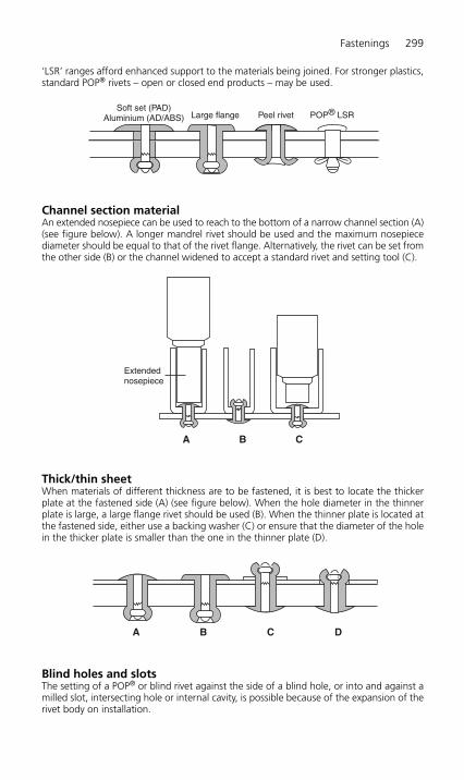
Fastenings 299
‘LSR’ ranges afford enhanced support to the materials being joined. For stronger plastics,standard POP® rivets – open or closed end products – may be used.
Channel section materialAn extended nosepiece can be used to reach to the bottom of a narrow channel section (A)(see figure below). A longer mandrel rivet should be used and the maximum nosepiecediameter should be equal to that of the rivet flange. Alternatively, the rivet can be set fromthe other side (B) or the channel widened to accept a standard rivet and setting tool (C).
Thick/thin sheetWhen materials of different thickness are to be fastened, it is best to locate the thickerplate at the fastened side (A) (see figure below). When the hole diameter in the thinnerplate is large, a large flange rivet should be used (B). When the thinner plate is located atthe fastened side, either use a backing washer (C) or ensure that the diameter of the holein the thicker plate is smaller than the one in the thinner plate (D).
Blind holes and slotsThe setting of a POP® or blind rivet against the side of a blind hole, or into and against amilled slot, intersecting hole or internal cavity, is possible because of the expansion of therivet body on installation.
A B C D
A B C
Extendednosepiece
POP® LSRLarge flange Peel rivetSoft set (PAD)
Aluminium (AD/ABS)
H6508-Ch04.2.qxd 9/12/05 4:46 PM Page 299
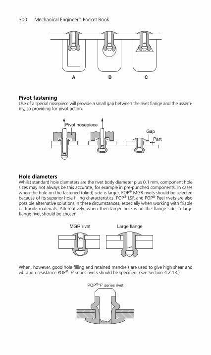
300 Mechanical Engineer’s Pocket Book
Pivot fasteningUse of a special nosepiece will provide a small gap between the rivet flange and the assem-bly, so providing for pivot action.
Hole diametersWhilst standard hole diameters are the rivet body diameter plus 0.1 mm, component holesizes may not always be this accurate, for example in pre-punched components. In caseswhen the hole on the fastened (blind) side is larger, POP® MGR rivets should be selectedbecause of its superior hole filling characteristics. POP® LSR and POP® Peel rivets are alsopossible alternative solutions in these circumstances, especially when working with friableor fragile materials. Alternatively, when then larger hole is on the flange side, a largeflange rivet should be chosen.
When, however, good hole filling and retained mandrels are used to give high shear andvibration resistance POP® ‘F’ series rivets should be specified. (See Section 4.2.13.)
POP® 'F' series rivet
MGR rivet Large flange
Pivot nosepieceGap
Part
A B C
H6508-Ch04.2.qxd 9/12/05 4:46 PM Page 300
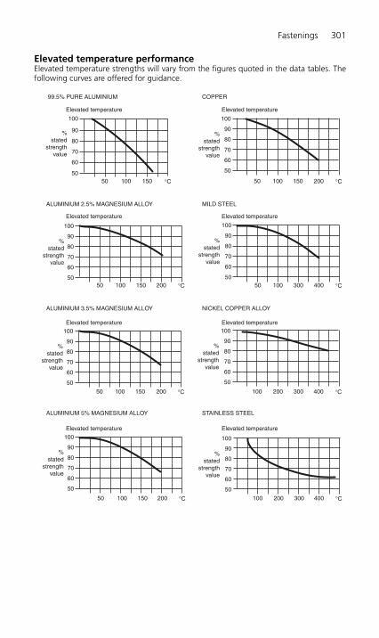
Fastenings 301
Elevated temperature performanceElevated temperature strengths will vary from the figures quoted in the data tables. Thefollowing curves are offered for guidance.
99.5% PURE ALUMINIUM
Elevated temperature
Elevated temperature
Elevated temperature
100
90
80
70
60
50
100
90
80
70
60
50
50 100 150 °C
50 100 150 200 °C
50 100 150 200 °C
%stated
strengthvalue
%stated
strengthvalue
100
90
80
70
60
50
%stated
strengthvalue
Elevated temperature
50 100 150 200 °C
100
90
80
70
60
50
%stated
strengthvalue
Elevated temperature
100 200 300 400 °C
100
90
80
70
60
50
%stated
strengthvalue
Elevated temperature
100 200 300 400 °C
100
90
80
70
60
50
%stated
strengthvalue
Elevated temperature
50 100 300 400 °C
100
90
80
70
60
50
%stated
strengthvalue
Elevated temperature
50 100 150 200 °C
100
90
80
70
60
50
%stated
strengthvalue
ALUMINIUM 2.5% MAGNESIUM ALLOY
ALUMINIUM 3.5% MAGNESIUM ALLOY
ALUMINIUM 5% MAGNESIUM ALLOY STAINLESS STEEL
NICKEL COPPER ALLOY
MILD STEEL
COPPER
H6508-Ch04.2.qxd 9/12/05 4:46 PM Page 301
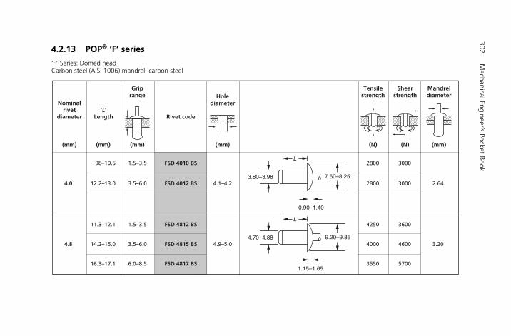
302M
echanical Engineer’s Pocket Book
4.2.13 POP® ‘F’ series
‘F’ Series: Domed headCarbon steel (AISI 1006) mandrel: carbon steel
7.60–8.253.80–3.98
0.90–1.40
L
9.20–9.854.70–4.88
1.15–1.65
L
Rivet code
Tensilestrength
(N)
Shearstrength
(N)
Mandreldiameter
(mm)
Holediameter
(mm)
Nominalrivet
diameter
(mm)
Griprange
(mm)(mm)
‘L’Length
98–10.6 1.5–3.5
12.2–13.0 3.5–6.0
1.5–3.5
3.5–6.0
11.3–12.1
14.2–15.0
16.3–17.1 6.0–8.5
4.0
4.8
4.1–4.2
4.9–5.0
2800 3000
3000
3600
4600
5700
2800
4250
4000
3550
2.64
3.20
FSD 4010 BS
FSD 4012 BS
FSD 4812 BS
FSD 4815 BS
FSD 4817 BS
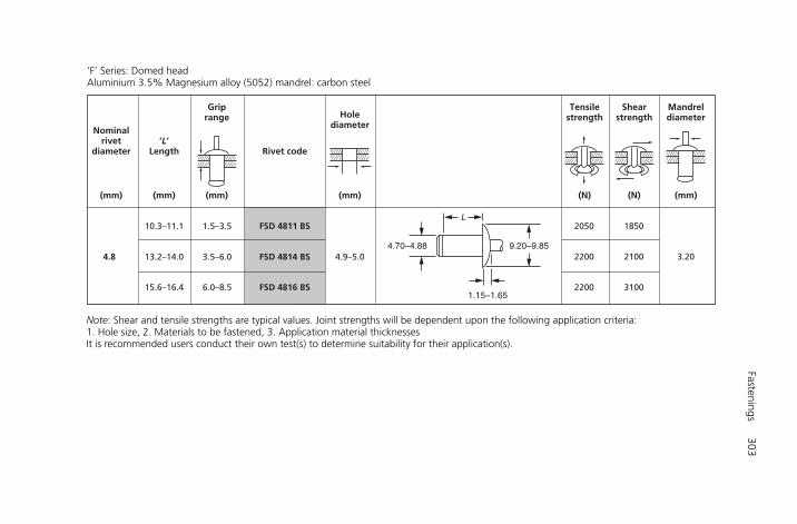
Fastenings303
‘F’ Series: Domed headAluminium 3.5% Magnesium alloy (5052) mandrel: carbon steel
Note: Shear and tensile strengths are typical values. Joint strengths will be dependent upon the following application criteria:1. Hole size, 2. Materials to be fastened, 3. Application material thicknessesIt is recommended users conduct their own test(s) to determine suitability for their application(s).
9.20–9.854.70–4.88
1.15–1.65
L
Rivet code
Tensilestrength
(N)
Shearstrength
(N)
Mandreldiameter
(mm)
Holediameter
(mm)
Nominalrivet
diameter
(mm)
Griprange
(mm)(mm)
‘L’Length
1.5–3.5
3.5–6.0
10.3–11.1
13.2–14.0
15.6–16.4 6.0–8.5
4.8 4.9–5.0
1850
2100
3100
2050
2200
2200
3.20
FSD 4811 BS
FSD 4814 BS
FSD 4816 BS
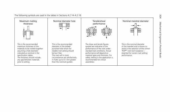
304M
echanical Engineer’s Pocket Book
The following symbols are used in the tables in Sections 4.2.14–4.2.16.
This is the recommended This is the recommended The shear and tensile figures This is the nominal diameter maximum thickness of the diameter of the drilled/ quoted are indicative of the of the mandrel and is shown to materials to be riveted together punched hole which for performance of the rivet under assist in the selection of the correctassuming a hole diameter reliable rivet setting should standard test conditions. Actual ‘POP®’ rivet tool nosepiece – indicated as nominal in the be burr free. performance will depend on essential for correct rivet setting specification tables. The rivet will in most material types and thickness. For performance.The thickness should include circumstances set satisfactorily safety, testing in the application is any gap between materials in holes up to 0.1 mm greater recommended for critical prior to setting. than the nominal quoted. assemblies.
Nominal diameter hole Tensile/shearperformance
Nominal mandrel diameterMaximum rivetingthickness
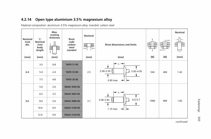
Fastenings305
4.2.14 Open type aluminium 3.5% magnesium alloy
Material composition: aluminium 3.5% magnesium alloy; mandrel: carbon steel
TAPD 31 BS
TAPD 33 BS
TAPD 36 BS
SNAD 3050 BS
SNAD 3065 BS
SNAD 3080 BS
SNAD 3100 BS
SNAD 3120 BS
Rivetcode
carbonsteel
mandrel
Nominal
(mm)
Rivet dimensions and limits
(mm)
Nominal
(mm)
Max.riveting
thickness
(mm)
2.4
3.0
‘L’Nominal
rivetbody
length
(mm)
Nominalrivetdia.
(mm) (N) (N)
3.5
7.5
6.5
2.5
3.1
3.5
5.0
5.0 2.0
4.8
0.8
2.4
8.0
9.0
6.0
5.0
10.0
12.0
3.08–2.90
1.10 max.
6.3–5.7
L
2.48–2.30 5.00–4.00
0.90 max.
L
550
1000 800
400 1.42
1.83
continued
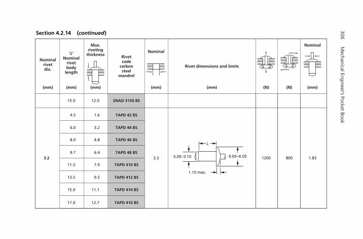
306M
echanical Engineer’s Pocket Book
6.65–6.053.28–3.10
1.10 max.
L
Rivetcode
carbonsteel
mandrel
(N) (N)
Nominal
(mm)
Nominal
(mm)
Rivet dimensions and limits
(mm)
Nominalrivetdia.
(mm)
Max.riveting
thickness
(mm)
‘L’Nominal
rivetbody
length
(mm)
15.0 12.0
4.5 1.6
3.26.0
8.0
9.7
11.5 7.9
13.5 9.5
15.0
17.0
3.2 3.3 1200 800 1.83
12.7
11.1
4.8
6.4
SNAD 3150 BS
TAPD 42 BS
TAPD 44 BS
TAPD 46 BS
TAPD 48 BS
TAPD 410 BS
TAPD 412 BS
TAPD 414 BS
TAPD 416 BS
Section 4.2.14 (continued)
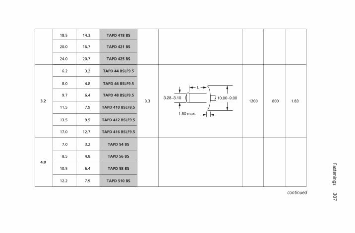
Fastenings307
10.00–9.003.28–3.10
1.50 max.
L
14.3
16.7
20.7
3.2
7.9
9.5
3.2
4.0
3.3 1200 800 1.83
3.2
4.8
6.4
7.9
18.5
20.0
24.0
6.2
8.0
9.7
11.5
13.5
7.0
8.5
10.5
12.2
17.0 12.7
6.4
4.8
TAPD 418 BS
TAPD 421 BS
TAPD 425 BS
TAPD 44 BSLF9.5
TAPD 46 BSLF9.5
TAPD 48 BSLF9.5
TAPD 410 BSLF9.5
TAPD 412 BSLF9.5
TAPD 416 BSLF9.5
TAPD 54 BS
TAPD 56 BS
TAPD 58 BS
TAPD 510 BS
continued
308M
echanical Engineer’s Pocket Book
Rivetcode
carbonsteel
mandrel
Rivet dimensions and limits (mm)
(N) (N)
Nominal
(mm)
Nominal
(mm)
Nominalrivetdia.
(mm)
Max.riveting
thickness
(mm)
‘L’Nominal
rivetbody
length
(mm)
14.0 9.5
15.7 11.1
12.717.5
18.5
20.2
22.5 17.4
24.7 19.8
8.5
10.5
4.0 4.1 1910 1330 2.29
6.4
4.8
13.5
15.9
TAPD 514 BS
TAPD 512 BS
TAPD 516 BS
TAPD 517 BS
TAPD 520 BS
TAPD 522 BS
TAPD 525 BS
TAPD 56 BSLF12
TAPD 58 BSLF12
8.22–7.624.08–3.90
1.35 max.
L
Section 4.2.14 (continued)
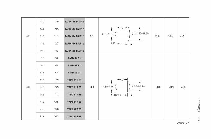
Fastenings309
12.2 7.9
9.514.0
15.7 11.1
17.5 12.7
19.4
7.5
9.2 4.8
11.0 6.4
4.0
4.8 4.9
4.1 1910 1330 2.29
2800 2020 2.6414.7 9.5
16.5 11.1
13.519.0
25.5 19.8
12.7 7.9
3.2
14.3 TAPD 518 BSLF12
TAPD 516 BSLF12
TAPD 514 BSLF12
TAPD 512 BSLF12
TAPD 510 BSLF12
TAPD 64 BS
TAPD 66 BS
TAPD 68 BS
TAPD 610 BS
TAPD 612 BS
TAPD 617 BS
TAPD 614 BS
TAPD 625 BS
TAPD 633 BS32.0 26.2
4.08–3.90
1.60 max.
L
12.150–11.50
4.88–4.70
1.60 max.
L
9.80–9.20
continued
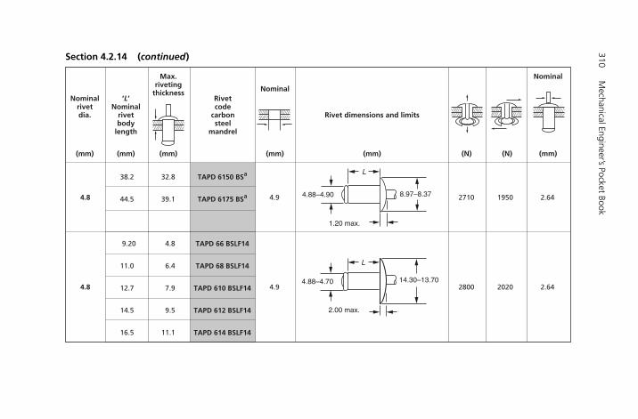
310M
echanical Engineer’s Pocket Book
Rivetcode
carbonsteel
mandrel
(N) (N)
Nominal
(mm)
Rivet dimensions and limits
(mm)
Nominal
(mm)
Nominalrivetdia.
(mm)
Max.riveting
thickness
(mm)
‘L’Nominal
rivetbody
length
(mm)
38.2 32.8
44.5 39.1
9.20
11.0
12.7 7.9
14.5 9.5
16.5
4.8
4.8
4.9
4.9
2710 1950 2.64
2800 2020 2.64
11.1
4.8
6.4
TAPD 6175 BSa
TAPD 6150 BSa
TAPD 66 BSLF14
TAPD 68 BSLF14
TAPD 610 BSLF14
TAPD 612 BSLF14
TAPD 614 BSLF14
4.88–4.70
2.00 max.
L
14.30–13.70
8.97–8.374.88–4.90
1.20 max.
L
Section 4.2.14 (continued)

Fastenings311
19.0
25.5 19.8
3.56.5
8.0 4.5
10.0 6.0
12.0
14.0
16.0 11.5
18.0 13.5
5.0
6.0
5.1 2600 2200 2.64
22.0 17.5
25.0 20.5
3.58.0
20.0 15.5
9.5
7.5
13.5
SNAD 5120 BS
SNAD 5100 BS
SNAD 5080 BS
SNAD 5065 BS
TAPD 625 BSLF14
SNAD 5140 BS
SNAD 5160 BS
SNAD 5180 BS
SNAD 5200 BS
SNAD 5220 BS
SNAD 6080 BS
SNAD 5250 BS
TAPD 617 BSLF14
5.08–4.85
1.60 max.
L
9.30–8.70
continued
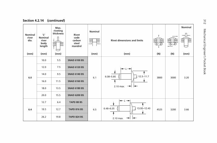
312M
echanical Engineer’s Pocket Book
Rivetcode
carbonsteel
mandrel
(N) (N)
Nominal
(mm)
Rivet dimensions and limits
(mm)
Nominal
(mm)
Nominalriverdia.
(mm)
Max.riveting
thickness
(mm)(mm)
‘L’Nominal
riverbody
length
12.3–11.76.08–5.85
2.10 max.
L
13.00–12.406.48–6.25
2.10 max.
L
3800 3000 3.20
4525 3200 3.66
10.0
12.0
14.0
16.0
18.0
20.0
12.7
12.7
19.8
19.5
26.2
11.5
13.5
15.5
6.4
9.5
7.5
5.5
6.0
6.4
6.1
6.5
SNAD 6100 BS
SNAD 6120 BS
SNAD 6140 BS
SNAD 6160 BS
SNAD 6180 BS
SNAD 6200 BS
TAPD 88 BS
TAPD 816 BS
TAPD 824 BS
Section 4.2.14 (continued)
Fastenings313
4.2.15 Open type carbon steel
Material composition: carbon steel; mandrel: carbon steel
Rivetcode
carbonsteel
mandrel
(N) (N)
Nominal
(mm)
Nominal
(mm)
Rivet dimensions and limits
(mm)
Nominalrivetdia.
(mm)
Max.riveting
thickness
(mm)
‘L’Nominal
rivetbody
length
(mm)
5.84–5.242.88–2.90
1.32 max.
L
6.3–5.73.08–2.90
1.1 max.
L
930 715 1.83
1400 1100 1.83
5.3
5.0
6.5
8.0
7.0
9.0
10.0
12.0
2.0
3.5
5.0
2.92.8
3.0
2.9
3.1
SNSD 3050 BS
SNSD 3080 BS
TSPD 33 BS
SNSD 3100 BS
SNSD 3120 BS
SNSD 3065 BS
continued
314M
echanical Engineer’s Pocket Book
Nominalrivetdia.
Rivetcode
carbonsteel
mandrel
(N) (N)
Nominal
(mm)
Rivet dimensions and limits
(mm)
Nominal
(mm)
Max.riveting
thickness
(mm)
‘L’Nominal
rivetbody
length.
(mm)(mm)
6.65–6.053.28–3.10
1.10 max.
L
1550 1150 1.93
15.0
4.5
6.0
8.0
9.5
11.5
13.5
1.65.0
4.8
6.4
7.9
9.5
3.2
1.6
12.0
3.2 3.3
SNAD 3150 BS*
TSPD 412 BS
TSPD 48 BS
TSPD 42 BS
TSPD 44 BS
TSPD 46 BS
TSPD 410 BS
TSPD 52 BS
3.27.0 TSPD 54 BS
Section 4.2.15 (continued)
Fastenings315
8.12–7.724.08–3.85
1.35 max.
L
9.82–9.224.88–4.65
1.60 max.
L
2500 1730 2.29
3500 2620 2.9
8.5 4.8
6.410.5
12.2 7.9
14.0 9.5
6.5 2.4
9.0 4.8
11.0 6.4
12.7 7.9
14.5 9.5
16.5 11.1
18.3 12.7
19.0 13.5
7.5 3.2
4.0
4.8
4.1
4.9
TSPD 56 BS
TSPD 58 BS
TSPD 510 BS
TSPD 512 BS
TSPD 63 BS
TSPD 64 BS
TSPD 66 BS
TSPD 68 BS
TSPD 610 BS
TSPD 612 BS
TSPD 614 BS
TSPD 616 BS
TSPD 617 BS
15.9 11.1
12.717.6
TSPD 514 BS
TSPD 516 BS
continued
316M
echanical Engineer’s Pocket Book
Rivetcode
carbonsteel
mandrel
(N) (N)
Nominal
(mm)
Rivet dimensions and limits
(mm)
Nominal
(mm)
Nominalrivetdia.
(mm)
Max.riveting
thickness
(mm)
‘L’Nominal
rivetbody
length
(mm)
9.30–8.705.08–4.85
1.6 max.
L
3790 2880 2.95.0 5.1
6.5 2.5 SNSD 5065 BS
8.0 4.0 SNSD 5080 BS
10.0 6.0 SNSD 5100 BS
12.0 8.0 SNSD 5120 BS
14.0 10.0 SNSD 5140 BS
16.0 12.0 SNSD 5160 BS
18.0 14.0 SNSD 5180 BS
4.010.0 SNSD 6100 BS
Section 4.2.15 (continued)

Fastenings317
12.3–11.76.08–5.85
2.1 max.
L
11.15–10.556.51–6.40
1.55 max.
L
5500 4200 3.65
6900 5000 3.86
6.012.0
6.0
6.4 6.5
6.1
SNSD 6120 BS
8.014.0 SNSD 6140 BS
10.016.0 SNSD 6160 BS
12.018.0 SNSD 6180 BS
3.89.5 TSPD 8095 BS
7.613.0 TSPD 8130 BS
12.718.5 TSPD 8185 BS
aBody �5% magnesium alloy.
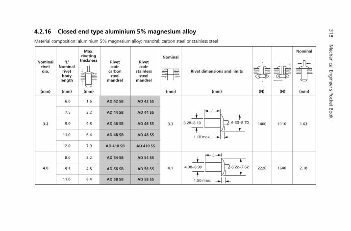
318M
echanical Engineer’s Pocket Book
4.2.16 Closed end type aluminium 5% magnesium alloy
Material composition: aluminium 5% magnesium alloy; mandrel: carbon steel or stainless steel
Rivetcode
carbonsteel
mandrel
Rivetcode
stainlesssteel
mandrel
(N) (N)
Nominal
(mm)
Rivet dimensions and limits
(mm)
Nominal
(mm)
Nominalrivetdia.
(mm)
Max.riveting
thickness
(mm)
‘L’Nominal
rivetbody
length
(mm)
6.30–5.703.28–3.10
1.10 max.
L
8.22–7.624.08–3.90
1.50 max.
L
1400 1110 1.63
2220 1640 2.18
6.0
7.5
9.0
11.0
12.0
8.0
9.5
6.411.0
6.4
7.9
3.2
4.8
4.8
3.2
1.6
3.2
4.0
3.3
4.1
AD 42 SB
AD 44 SB
AD 46 SB
AD 48 SB
AD 410 SB
AD 54 SB
AD 56 SB
AD 58 SB
AD 42 SS
AD 44 SS
AD 46 SS
AD 48 SS
AD 410 SS
AD 54 SS
AD 56 SS
AD 58 SS

Fastenings319
9.85–9.204.88–4.70
1.75 max.
L
3110 2260 2.64
4800 4000 3.66
7.912.5
4.8
6.4
4.9
6.5
AD 510 SB
3.28.30 AD 64 SB
4.810.0 AD 66 SB
6.411.5 AD 68 SB
7.913.0 AD 610 SB
9.514.5 AD 612 SB
12.718.0 AD 616 SB
15.922.0 AD 620 SB
AD 510 SS
AD 64 SS
AD 66 SS
AD 68 SS
AD 610 SS
AD 612 SS
AD 616 SS
AD 620 SS
6.413.0 AD 84 H
9.516.0 AD 86 H
–
–
13.34–12.066.48–6.32
2.51 max.
L
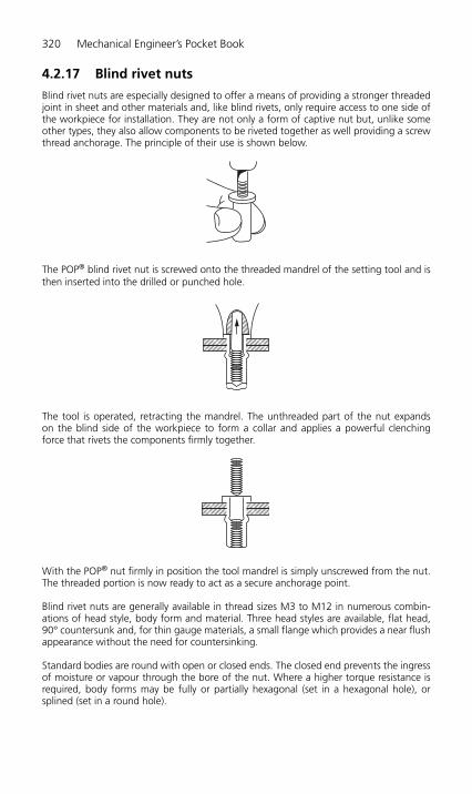
320 Mechanical Engineer’s Pocket Book
4.2.17 Blind rivet nuts
Blind rivet nuts are especially designed to offer a means of providing a stronger threadedjoint in sheet and other materials and, like blind rivets, only require access to one side ofthe workpiece for installation. They are not only a form of captive nut but, unlike someother types, they also allow components to be riveted together as well providing a screwthread anchorage. The principle of their use is shown below.
The POP® blind rivet nut is screwed onto the threaded mandrel of the setting tool and isthen inserted into the drilled or punched hole.
The tool is operated, retracting the mandrel. The unthreaded part of the nut expands on the blind side of the workpiece to form a collar and applies a powerful clenching force that rivets the components firmly together.
With the POP® nut firmly in position the tool mandrel is simply unscrewed from the nut.The threaded portion is now ready to act as a secure anchorage point.
Blind rivet nuts are generally available in thread sizes M3 to M12 in numerous combin-ations of head style, body form and material. Three head styles are available, flat head,90° countersunk and, for thin gauge materials, a small flange which provides a near flushappearance without the need for countersinking.
Standard bodies are round with open or closed ends. The closed end prevents the ingressof moisture or vapour through the bore of the nut. Where a higher torque resistance isrequired, body forms may be fully or partially hexagonal (set in a hexagonal hole), orsplined (set in a round hole).
H6508-Ch04.2.qxd 9/12/05 4:46 PM Page 320
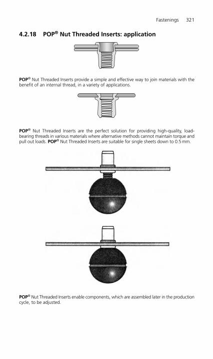
Fastenings 321
4.2.18 POP® Nut Threaded Inserts: application
POP® Nut Threaded Inserts provide a simple and effective way to join materials with thebenefit of an internal thread, in a variety of applications.
POP® Nut Threaded Inserts are the perfect solution for providing high-quality, load-bearing threads in various materials where alternative methods cannot maintain torque andpull out loads. POP® Nut Threaded Inserts are suitable for single sheets down to 0.5 mm.
POP® Nut Threaded Inserts enable components, which are assembled later in the productioncycle, to be adjusted.
H6508-Ch04.2.qxd 9/12/05 4:46 PM Page 321

322 Mechanical Engineer’s Pocket Book
POP® Nut Threaded Inserts are ideally suited to applications where access is only availablefrom one side of the workpiece.
4.2.19 POP® Nut Threaded Inserts: installation
POP® Nut Threaded Inserts are easily installed from one side of the workpiece withoutdamaging surrounding surfaces of previously finished or delicate components and aresuitable for use with all materials in today’s manufacturing environment:
● Available in a variety of materials● Wide range of styles● Complete range of Hand and Power setting tools● Bulk and small pack available.
Install/screw the POP® Nut Threaded Insert to the tool’s threaded mandrel.
Operating the tool then retracts the mandrel. The unthreaded part of the nut then com-presses to form a collar on the blind side of the workpiece, applying a powerful clenchingforce that firmly joins the components together.
H6508-Ch04.2.qxd 9/12/05 4:46 PM Page 322

Fastenings 323
With the POP® Nut Threaded Insert firmly in position, the tool mandrel is simplydemounted/unscrewed from the insert.
The threaded part of the insert then acts as a secure anchorage point for subsequentassembly work.
H6508-Ch04.2.qxd 9/12/05 4:46 PM Page 323
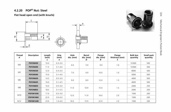
324M
echanical Engineer’s Pocket Book4.2.20 POP® Nut: Steel
Flat head open end (with knurls)
Thread Description Length Grip Hole Barrel Flange Flange Bulk box Small pack d (mm) (mm) dia. (mm) dia. (mm) dia. (mm) thickness (mm) quantity quantity
L e D B S
M4PSFON430 10.0 0.3–3.0
6.0 5.9 9.0 1.010 000 500
PSFON440 11.5 3.1–4.0 10 000 500
M5PSFON530 12.0 0.3–3.0
7.0 6.9 10.0 1.08000 500
PSFON540 15.0 3.1–4.0 5000 500
M6PSFON630 14.5 0.5–3.0
9.0 8.9 12.0 1.54000 500
PSFON645 16.0 3.1–4.5 4000 500
M8PSFON830 16.0 0.5–3.0
11.0 10.9 15.0 1.52000 250
PSFON855 18.5 3.1–5.5 2000 250
M10PSFON1030 17.0 0.5–3.0
12.0 11.9 16.0 2.01500 200
PSFON1060 22.0 3.0–6.0 1500 200
M12 PSFON1240 23.0 1.0–4.0 16.0 15.9 22.0 2.0 1500 200
L
B d D
S
e

Fastenings325
Thread Description Length Grip Hole Barrel Flange Flange Bulk box Small pack d (mm) (mm) dia. (mm) dia. (mm) dia. (mm) thickness (mm) quantity quantity
L e D B S
M5 PSFCN530 18.0 0.3–3.0 7.0 6.9 10.0 1.0 5000 500
M6 PSFCN630 20.5 0.5–3.0 9.0 8.9 12.0 1.5 2000 500
M8 PSFCN830 25.0 0.5–3.0 11.0 10.9 15.0 1.5 1500 250
L
B
S
d D
e
Flat head closed end (with knurls)
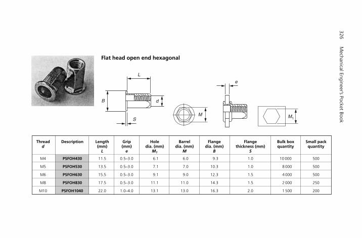
326M
echanical Engineer’s Pocket Book
Flat head open end hexagonal
Thread Description Length Grip Hole Barrel Flange Flange Bulk box Small pack d (mm) (mm) dia. (mm) dia. (mm) dia. (mm) thickness (mm) quantity quantity
L e M1 M B S
M4 PSFOH430 11.5 0.5–3.0 6.1 6.0 9.3 1.0 10 000 500
M5 PSFOH530 13.5 0.5–3.0 7.1 7.0 10.3 1.0 8 000 500
M6 PSFOH630 15.5 0.5–3.0 9.1 9.0 12.3 1.5 4 000 500
M8 PSFOH830 17.5 0.5–3.0 11.1 11.0 14.3 1.5 2 000 250
M10 PSFOH1040 22.0 1.0–4.0 13.1 13.0 16.3 2.0 1 500 200
L
B
S
d
M
e
M1

Fastenings327
Countersunk head open end (with knurls)
Thread Description Length Grip Hole Barrel Flange Flange Bulk box Small pack d (mm) (mm) dia. (mm) dia. (mm) dia. (mm) thickness (mm) quantity quantity
L e D B S
M4 PSKON435 11.5 2.0–3.5 6.0 5.9 9.0 1.5 10 000 500
M5 PSKON540 13.5 2.0–4.0 7.0 6.9 10.0 1.5 8 000 500
M6 PSKON645 16.0 2.0–4.5 9.0 8.9 12.0 1.5 4 000 500
M8 PSKON845 19.0 2.0–4.5 11.0 10.9 14.0 1.5 2 000 250
M10 PSKON1045 21.0 2.0–4.5 12.0 11.9 14.7 1.5 1 500 200
L
B
S
d D90°
e
For further information see the wide range of publications concerning POP® riveting issued by Emhart Teknologies (Tucker Fasteners Ltd) – See Appendix 3.
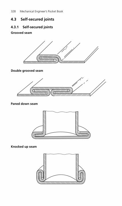
328 Mechanical Engineer’s Pocket Book
4.3 Self-secured joints
4.3.1 Self-secured joints
Grooved seam
Double grooved seam
Paned down seam
Knocked up seam
H6508-Ch04.3.qxd 9/12/05 4:46 PM Page 328
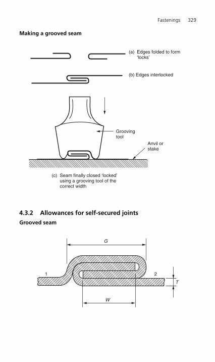
Making a grooved seam
4.3.2 Allowances for self-secured joints
Grooved seam
1 2
G
W
T
(a) Edges folded to form ‘locks’
(b) Edges interlocked
Groovingtool
(c) Seam finally closed ‘locked’ using a grooving tool of the correct width
Anvil orstake
Fastenings 329
H6508-Ch04.3.qxd 9/12/05 4:46 PM Page 329
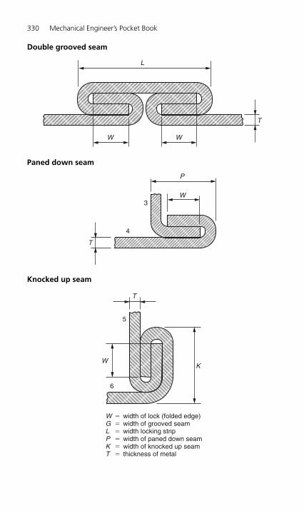
330 Mechanical Engineer’s Pocket Book
Double grooved seam
Paned down seam
Knocked up seam
W
W � width of lock (folded edge)G � width of grooved seamL � width locking stripP � width of paned down seamK � width of knocked up seamT � thickness of metal
K
T
5
6
W
P
T
3
4
W W
L
T
H6508-Ch04.3.qxd 9/12/05 4:46 PM Page 330
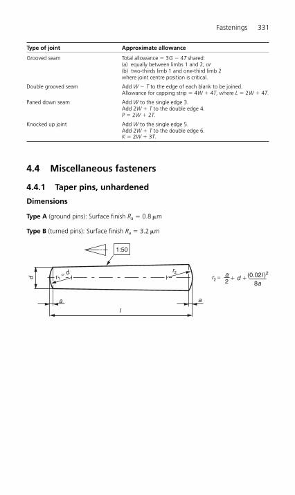
Type of joint Approximate allowance
Grooved seam Total allowance � 3G � 4T shared:(a) equally between limbs 1 and 2; or(b) two-thirds limb 1 and one-third limb 2where joint centre position is critical.
Double grooved seam Add W � T to the edge of each blank to be joined.Allowance for capping strip � 4W � 4T, where L � 2W � 4T.
Paned down seam Add W to the single edge 3.Add 2W � T to the double edge 4.P � 2W � 2T.
Knocked up joint Add W to the single edge 5.Add 2W � T to the double edge 6.K � 2W � 3T.
4.4 Miscellaneous fasteners
4.4.1 Taper pins, unhardened
Dimensions
Type A (ground pins): Surface finish Ra � 0.8 �m
Type B (turned pins): Surface finish Ra � 3.2 �m
1:50
a a
d r1 ≈ d r2
r2 ≈a2 � d �
8a(0.02l )2
l
Fastenings 331
H6508-Ch04.3.qxd 9/12/05 4:46 PM Page 331
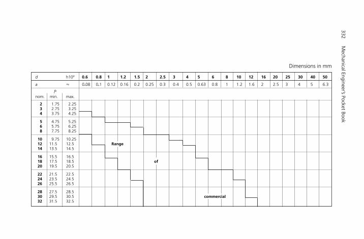
332M
echanical Engineer’s Pocket Book
Dimensions in mm
d h10a 0.6 0.8 1 1.2 1.5 2 2.5 3 4 5 6 8 10 12 16 20 25 30 40 50
a � 0.08 0.1 0.12 0.16 0.2 0.25 0.3 0.4 0.5 0.63 0.8 1 1.2 1.6 2 2.5 3 4 5 6.3
lb
nom. min. max.
2 1.75 2.253 2.75 3.254 3.75 4.25
5 4.75 5.256 5.75 6.258 7.75 8.25
10 9.75 10.2512 11.5 12.5 Range14 13.5 14.5
16 15.5 16.518 17.5 18.5 of20 19.5 20.5
22 21.5 22.524 23.5 24.526 25.5 26.5
28 27.5 28.530 29.5 30.5 commercial32 31.5 32.5

Fastenings333
35 34.5 35.540 39.5 40.545 44.5 45.5
50 49.5 50.555 54.25 55.7560 59.25 60.75
65 64.25 65.7570 69.25 70.75 lengths75 74.25 75.75
80 79.25 80.7585 84.25 85.7590 89.25 90.75
95 94.25 95.75100 99.25 100.75120 119.25 120.75
140 139.25 140.75160 159.25 160.75180 179.25 180.75200 199.25 200.75
aOther tolerances, for example, a11, c11, f8, as agreed between customer and supplier.bFor nominal lengths above 200 mm, steps of 20 mm.

Specifications and reference International Standards
Material St � Free-cutting steel, hardness 125 to 245 HV.Other materials as agreed between customer and supplier.
Surface finish Plain, that is, pins to be supplied in natural finish treated with a rust-preventative lubricant,unless otherwise specified by agreement between customer and supplier.
Preferred coatings are black oxide, phosphate coating or zinc plating with chromate conversioncoating (see ISO 2081 and ISO 4520).Other coatings as agreed between customer and supplier.All tolerances shall apply prior to the application of a plating or coating.
Workmanship Parts shall be uniform in quality and free of irregularities or detrimental defects.No burrs shall appear on any part of the pin.
Taper The taper shall be inspected by use of an adequate optical comparator.
Acceptability The acceptance procedure is covered in ISO 3269.
DesignationExample for the designation of an unhardened steel taper pin, type A, with nominal diameterd � 6 mm and nominal length l � 30 mm:
Taper pin ISO 2339 – A – 6 � 30 – St
334M
echanical Engineer’s Pocket Book
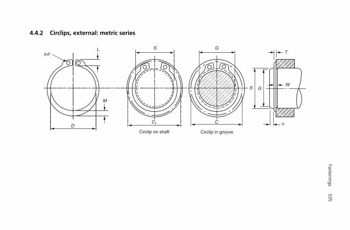
Fastenings335
4.4.2 Circlips, external: metric series
D
M
L S
S
C1 C
G
G
T
W
n
fd
Circlip on shaft Circlip in groove
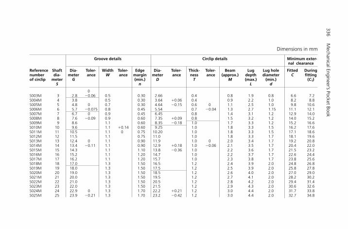
336M
echanical Engineer’s Pocket Book
Dimensions in mm
Groove details Circlip details Minimum exter-nal clearance
Reference Shaft Dia- Toler- Width Toler- Edge Dia- Toler- Thick- Toler- Beam Lug Lug hole Fitted During number dia- meter ance W ance margin meter ance ness ance (approx.) depth diameter C fitting of circlip meter G (min.) D T M (max.) (min.) (C1)
S n L d
0S003M 3 2.8 �0.06 0.5 0.30 2.66 0.4 0.8 1.9 0.8 6.6 7.2S004M 4 3.8 0.5 0.30 3.64 �0.06 0.4 0.9 2.2 1.0 8.2 8.8S005M 5 4.8 0 0.7 0.30 4.64 �0.15 0.6 0 1.1 2.5 1.0 9.8 10.6S006M 6 5.7 �0.075 0.8 0.45 5.54 0.7 �0.04 1.3 2.7 1.15 11.1 12.1S007M 7 6.7 0 0.9 0.45 6.45 0.8 1.4 3.1 1.2 12.9 14.0S008M 8 7.6 �0.09 0.9 0.60 7.35 �0.09 0.8 1.5 3.2 1.2 14.0 15.2S009M 9 8.6 1.1 0.60 8.35 �0.18 1.0 1.7 3.3 1.2 15.2 16.6S010M 10 9.6 1.1 �0.14 0.60 9.25 1.0 1.8 3.3 1.5 16.2 17.6S011M 11 10.5 1.1 0 0.75 10.20 1.0 1.8 3.3 1.5 17.1 18.6S012M 12 11.5 1.1 0.75 11.0 1.0 1.8 3.3 1.7 18.1 19.6S013M 13 12.4 0 1.1 0.90 11.9 1.0 0 2.0 3.4 1.7 19.2 20.8S014M 14 13.4 �0.11 1.1 0.90 12.9 �0.18 1.0 �0.06 2.1 3.5 1.7 20.4 22.0S015M 15 14.3 1.1 1.10 13.8 �0.36 1.0 2.2 3.6 1.7 21.5 23.2S016M 16 15.2 1.1 1.20 14.7 1.0 2.2 3.7 1.7 22.6 24.4S017M 17 16.2 1.1 1.20 15.7 1.0 2.3 3.8 1.7 23.8 25.6S018M 18 17.0 1.3 1.50 16.5 1.2 2.4 3.9 2.0 24.8 26.8S019M 19 18.0 1.3 1.50 17.5 1.2 2.5 3.9 2.0 25.8 27.8S020M 20 19.0 1.3 1.50 18.5 1.2 2.6 4.0 2.0 27.0 29.0S021M 21 20.0 1.3 1.50 19.5 1.2 2.7 4.1 2.0 28.2 30.2S022M 22 21.0 1.3 1.50 20.5 1.2 2.8 4.2 2.0 29.4 31.4S023M 23 22.0 1.3 1.50 21.5 1.2 2.9 4.3 2.0 30.6 32.6S024M 24 22.9 0 1.3 1.70 22.2 �0.21 1.2 3.0 4.4 2.0 31.7 33.8S025M 25 23.9 �0.21 1.3 1.70 23.2 �0.42 1.2 3.0 4.4 2.0 32.7 34.8
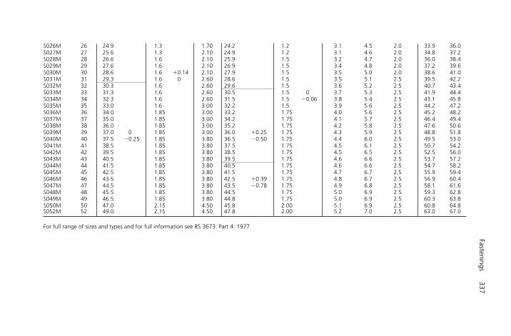
Fastenings337
S026M 26 24.9 1.3 1.70 24.2 1.2 3.1 4.5 2.0 33.9 36.0S027M 27 25.6 1.3 2.10 24.9 1.2 3.1 4.6 2.0 34.8 37.2S028M 28 26.6 1.6 2.10 25.9 1.5 3.2 4.7 2.0 36.0 38.4S029M 29 27.6 1.6 2.10 26.9 1.5 3.4 4.8 2.0 37.2 39.6S030M 30 28.6 1.6 �0.14 2.10 27.9 1.5 3.5 5.0 2.0 38.6 41.0S031M 31 29.3 1.6 0 2.60 28.6 1.5 3.5 5.1 2.5 39.5 42.2S032M 32 30.3 1.6 2.60 29.6 1.5 3.6 5.2 2.5 40.7 43.4S033M 33 31.3 1.6 2.60 30.5 1.5 0 3.7 5.3 2.5 41.9 44.4S034M 34 32.3 1.6 2.60 31.5 1.5 �0.06 3.8 5.4 2.5 43.1 45.8S035M 35 33.0 1.6 3.00 32.2 1.5 3.9 5.6 2.5 44.2 47.2S036M 36 34.0 1.85 3.00 33.2 1.75 4.0 5.6 2.5 45.2 48.2S037M 37 35.0 1.85 3.00 34.2 1.75 4.1 5.7 2.5 46.4 49.4S038M 38 36.0 1.85 3.00 35.2 1.75 4.2 5.8 2.5 47.6 50.6S039M 39 37.0 0 1.85 3.00 36.0 �0.25 1.75 4.3 5.9 2.5 48.8 51.8S040M 40 37.5 �0.25 1.85 3.80 36.5 �0.50 1.75 4.4 6.0 2.5 49.5 53.0S041M 41 38.5 1.85 3.80 37.5 1.75 4.5 6.1 2.5 50.7 54.2S042M 42 39.5 1.85 3.80 38.5 1.75 4.5 6.5 2.5 52.5 56.0S043M 43 40.5 1.85 3.80 39.5 1.75 4.6 6.6 2.5 53.7 57.2S044M 44 41.5 1.85 3.80 40.5 1.75 4.6 6.6 2.5 54.7 58.2S045M 45 42.5 1.85 3.80 41.5 1.75 4.7 6.7 2.5 55.9 59.4S046M 46 43.5 1.85 3.80 42.5 �0.39 1.75 4.8 6.7 2.5 56.9 60.4S047M 47 44.5 1.85 3.80 43.5 �0.78 1.75 4.9 6.8 2.5 58.1 61.6S048M 48 45.5 1.85 3.80 44.5 1.75 5.0 6.9 2.5 59.3 62.8S049M 49 46.5 1.85 3.80 44.8 1.75 5.0 6.9 2.5 60.3 63.8S050M 50 47.0 2.15 4.50 45.8 2.00 5.1 6.9 2.5 60.8 64.8S052M 52 49.0 2.15 4.50 47.8 2.00 5.2 7.0 2.5 63.0 67.0
For full range of sizes and types and for full information see BS 3673: Part 4: 1977.

338M
echanical Engineer’s Pocket Book
4.4.3 Circlips, internal: metric series
D
L
M
B
Circlip in bore Circlip in groove
C1 C
G
G B
T
W
n
fd
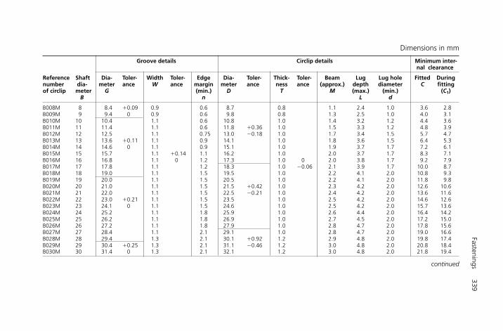
Fastenings339
Dimensions in mm
Groove details Circlip details Minimum inter-nal clearance
Reference Shaft Dia- Toler- Width Toler- Edge Dia- Toler- Thick- Toler- Beam Lug Lug hole Fitted During number dia- meter ance W ance margin meter ance ness ance (approx.) depth diameter C fitting of circlip meter G (min.) D T M (max.) (min.) (C1)
B n L d
B008M 8 8.4 �0.09 0.9 0.6 8.7 0.8 1.1 2.4 1.0 3.6 2.8B009M 9 9.4 0 0.9 0.6 9.8 0.8 1.3 2.5 1.0 4.0 3.1B010M 10 10.4 1.1 0.6 10.8 1.0 1.4 3.2 1.2 4.4 3.6B011M 11 11.4 1.1 0.6 11.8 �0.36 1.0 1.5 3.3 1.2 4.8 3.9B012M 12 12.5 1.1 0.75 13.0 �0.18 1.0 1.7 3.4 1.5 5.7 4.7B013M 13 13.6 �0.11 1.1 0.9 14.1 1.0 1.8 3.6 1.5 6.4 5.3B014M 14 14.6 0 1.1 0.9 15.1 1.0 1.9 3.7 1.7 7.2 6.1B015M 15 15.7 1.1 �0.14 1.1 16.2 1.0 2.0 3.7 1.7 8.3 7.1B016M 16 16.8 1.1 0 1.2 17.3 1.0 0 2.0 3.8 1.7 9.2 7.9B017M 17 17.8 1.1 1.2 18.3 1.0 �0.06 2.1 3.9 1.7 10.0 8.7B018M 18 19.0 1.1 1.5 19.5 1.0 2.2 4.1 2.0 10.8 9.3B019M 19 20.0 1.1 1.5 20.5 1.0 2.2 4.1 2.0 11.8 9.8B020M 20 21.0 1.1 1.5 21.5 �0.42 1.0 2.3 4.2 2.0 12.6 10.6B021M 21 22.0 1.1 1.5 22.5 �0.21 1.0 2.4 4.2 2.0 13.6 11.6B022M 22 23.0 �0.21 1.1 1.5 23.5 1.0 2.5 4.2 2.0 14.6 12.6B023M 23 24.1 0 1.1 1.5 24.6 1.0 2.5 4.2 2.0 15.7 13.6B024M 24 25.2 1.1 1.8 25.9 1.0 2.6 4.4 2.0 16.4 14.2B025M 25 26.2 1.1 1.8 26.9 1.0 2.7 4.5 2.0 17.2 15.0B026M 26 27.2 1.1 1.8 27.9 1.0 2.8 4.7 2.0 17.8 15.6B027M 27 28.4 1.1 2.1 29.1 1.0 2.8 4.7 2.0 19.0 16.6B028M 28 29.4 1.3 2.1 30.1 �0.92 1.2 2.9 4.8 2.0 19.8 17.4B029M 29 30.4 �0.25 1.3 2.1 31.1 �0.46 1.2 3.0 4.8 2.0 20.8 18.4B030M 30 31.4 0 1.3 2.1 32.1 1.2 3.0 4.8 2.0 21.8 19.4
continued
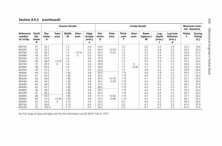
340M
echanical Engineer’s Pocket Book
Groove details Circlip details Minimum inter-nal clearance
Reference Shaft Dia- Toler- Width Toler- Edge Dia- Toler- Thick- Toler- Beam Lug Lug hole Fitted During number dia- meter ance W ance margin meter ance ness ance (approx.) depth diameter C fitting of circlip meter G (min.) D T M (max.) (min.) (C1)
B n L d
B031M 31 32.7 1.3 2.6 33.4 1.2 3.2 5.2 2.5 22.3 19.6B032M 32 33.7 1.3 2.6 34.4 �0.50 1.2 3.2 5.4 2.5 22.9 20.2B033M 33 34.7 1.3 �0.14 2.6 35.5 �0.25 1.2 3.3 5.4 2.5 23.9 21.2B034M 34 35.7 1.6 0 2.6 36.5 1.5 3.3 5.4 2.5 24.9 22.2B035M 35 37.0 1.6 3.0 37.8 1.5 3.4 5.4 2.5 26.2 23.2B036M 36 38.0 �0.25 1.6 3.0 38.8 1.5 3.5 5.4 2.5 27.2 24.2B037M 37 39.0 0 1.6 3.0 39.8 1.5 0 3.6 5.5 2.5 28.0 25.0B038M 38 40.0 1.6 3.0 40.8 1.5 �0.06 3.7 5.5 2.5 29.0 26.0B039M 39 41.0 1.6 3.0 42.0 1.5 3.8 5.6 2.5 29.8 26.8B040M 40 42.5 1.85 3.8 43.5 1.75 3.9 5.8 2.5 30.9 27.4B041M 41 43.5 1.85 3.8 44.5 1.75 4.0 5.9 2.5 31.7 28.2B042M 42 44.5 1.85 3.8 45.5 �0.78 1.75 4.1 5.9 2.5 32.7 29.2B043M 43 45.5 1.85 3.8 46.5 �0.39 1.75 4.2 6.0 2.5 33.5 30.0B044M 44 46.5 1.85 3.8 47.5 1.75 4.3 6.0 2.5 34.5 31.0B045M 45 47.5 1.85 3.8 48.5 1.75 4.3 6.2 2.5 35.1 31.6B046M 46 48.5 1.85 3.8 49.5 1.75 4.4 6.3 2.5 35.9 32.4B047M 47 49.5 1.85 3.8 50.5 1.75 4.4 6.4 2.5 36.7 33.2B048M 48 50.5 1.85 3.8 51.5 �0.92 1.75 4.5 6.4 2.5 37.7 34.2B049M 49 51.5 �0.30 1.85 3.8 52.5 �0.46 1.75 4.5 6.4 2.5 38.7 35.2B050M 50 53.0 0 2.15 4.5 54.2 2.0 4.6 6.5 2.5 40.0 36.0B051M 51 54.0 2.15 4.5 55.2 2.0 4.7 6.5 2.5 41.0 37.0B052M 52 555.0 2.15 4.5 56.2 2.0 4.7 6.7 2.5 41.6 37.6
For full range of sizes and types and for full information see BS 3673: Part 4: 1977.
Section 4.4.3 (continued )

Fastenings 341
4.5 Adhesive bonding of metals
4.5.1 Anaerobic adhesives
These are high-strength adhesives widely used in the engineering industry. Anaerobic adhe-sives are single-compound materials that remain inactive when in contact with oxygen. Theadhesives require two conditions to be present simultaneously in order to cure. That is, theabsence of oxygen and in the presence of metal parts. These adhesives are widely used forthreadlocking, threadsealing, gasketing and retaining (or cylindrical part bonding) at roomtemperature where ideal conditions exist for the adhesive to cure as shown in Fig. 1.
Figure 1 The adhesive flows into the spaces between the gear andthe shaft where it has the ideal conditions to cure (absence of oxygenand metal part activity).
Copper, brass and plain carbon steel are ‘active’ as far as anaerobic adhesives are con-cerned and result in rapid curing at normal room temperatures. Stainless steel, aluminiumand aluminium alloys, and plated products are ‘passive’ and require the use of an activa-tor to ensure a full cure. As a liquid, the adhesive flows into the interstitial spaces betweenthe male and female components of the joint where, devoid of atmospheric oxygen, itcures and becomes ‘keyed’ to the surface roughness. The curing process is also stimulatedby contact between the adhesive and the metal surface that acts as a catalyst in the caseof ‘active’. Once cured to provide a tough thermoset plastic, the adhesive provides up to60% of the torsional strength of the joint as shown in Fig. 2. To ensure a successful jointthe mating surfaces must be mechanically and chemically clean before applying the adhe-sive and any activator necessary – normally to the male component for convenience.Handling strength is achieved within 10–20 min of the joint being achieved and fullstrength is attained in 4–24 h depending on the gap between the mating components,the materials being joined and the temperature. The cured adhesives will resist tempera-tures up to 150°C and are resistant to most chemicals, although some higher tempera-ture versions are available. Typical anaerobic adhesives from the Loctite product range andsome applications are listed in Table 1.
4.5.2 Adhesives cured by ultraviolet light
These are adhesives that are cured by the application of ultraviolet (UV) light. The cure timesdepend on the intensity and wavelength of the UV light which initiates polymerization.
Note: Suitable eye-protection should always be used when working with UV light.
H6508-Ch04.3.qxd 9/12/05 4:47 PM Page 341
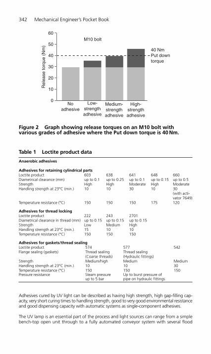
342 Mechanical Engineer’s Pocket Book
Adhesives cured by UV light can be described as having high strength, high gap-filling cap-acity, very short curing times to handling strength, good to very good environmental resistanceand good dispensing capacity with automatic systems as single-component adhesives.
The UV lamp is an essential part of the process and light sources can range from a simplebench-top open unit through to a fully automated conveyor system with several flood
60
50R
elea
se to
rque
(N
m)
40 NmPut downtorque
M10 bolt
40
30
20
10
0No
adhesiveLow-
strengthadhesive
Medium-strengthadhesive
High-strengthadhesive
Figure 2 Graph showing release torques on an M10 bolt with various grades of adhesive where the Put down torque is 40 Nm.
Table 1 Loctite product data
Anaerobic adhesives
Adhesives for retaining cylindrical partsLoctite product 603 638 641 648 660Diametrical clearance (mm) up to 0.1 up to 0.25 up to 0.1 up to 0.15 up to 0.5Strength High High Moderate High ModerateHandling strength at 23°C (min.) 10 10 30 10 30
(with acti-vator 7649)
Temperature resistance (°C) 150 150 150 175 120
Adhesives for thread lockingLoctite product 222 243 2701Diametrical clearance in thread (mm) up to 0.15 up to 0.15 up to 0.15Strength Low Medium HighHandling strength at 23°C (min.) 15 10 10Temperature resistance (°C) 150 150 150
Adhesives for gaskets/thread sealingLoctite product 574 577 542Flange sealing (gaskets) Thread sealing Thread sealing
(Coarse threads) (Hydraulic fittings)Strength Medium/high Medium MediumHandling strength at 23°C (min.) 10 10 30Temperature resistance (°C) 150 150 150Pressure resistance Steam pressure Up to burst pressure of
up to 5 bar pipe on hydraulic fittings
H6508-Ch04.3.qxd 9/12/05 4:47 PM Page 342

lights, incorporating special fixturing to hold the components in place during the curingcycle. UV light guides (or ‘wand’ systems) are often specified for small components asthese units produce high-intensity light over a diameter of about 10 mm. These lightguides ensure that the UV light is directed to the precise area for curing, thus minimizingglare and stray UV light. An example of a light guide is shown in the following figure.
In some applications, it is not always possible to ensure that the entire adhesive is exposedto the UV light and products are available which will cure after the UV cycle. There areseveral options for the secondary cure as follows.
HeatA secondary heat cure will ensure the full cure of many grades of UV adhesives. Cure tem-peratures are typically in the range 100–150°C.
AnaerobicUV anaerobic grades are available for applications where a shadow cure is required. Theseanaerobic adhesives will cure through a depth of 0.2 mm due to contact with metal partsand the absence of oxygen.
MoistureUV silicone products will immobilize after UV cure and then continue to cure over 24 hdue to surrounding atmospheric moisture.
Surface moistureUV curing cyanoacrylates will cure through several millimetres with UV light but also curedue to surface moisture in shadowed areas.
Fastenings 343
A flexible UV light guide unit for curing UV adhesives.
H6508-Ch04.3.qxd 9/12/05 4:47 PM Page 343

344 Mechanical Engineer’s Pocket Book
One of the main reasons why UV adhesives are used is the benefit of ‘cure on demand’(i.e. the ability to cure the product exactly when required once, and not until, the com-ponents are fully aligned).
4.5.3 Adhesives cured by anionic reaction (cyanoacrylates)
Single-component cyanoacrylate adhesives polymerize on contact with slightly alkalinesurfaces. In general, ambient humidity in the air and on the bonding surface is sufficientto initiate curing to handing strength within a few seconds. The best results are achievedwhen the relative humidity value is 40–60% at the workplace at room temperature.Lower humidity leads to slower curing, higher humidity accelerates the curing but inextreme cases may impair the final strength of the bond.
After adhesive application, the parts must be assembled quickly since polymerizationbegins in only a few seconds. The open time is dependent on the relative humidity, thehumidity of the bonding surfaces and the ambient temperature. Due to their very fast cur-ing times, cyanoacrylate adhesives are particularly suitable for bonding small parts. UVcuring grades are also available to improve the cure throughout the depth of the adhesiveand to cure any excess adhesive. Cyanoacrylate adhesives should be applied only to onesurface and the best bond is achieved if only enough adhesive is applied to fill the jointgap. Activators may be used to speed the curing process and to cure any excess adhesive.A further benefit of cyanoacrylates is that they can be used with primers to bond low-energy plastics such as polypropylene and polyethylene.
Features of cyanoacrylate adhesives are:
● very high shear and tensile strength;● very fast curing speed (seconds rather than minutes);● minimum adhesive consumption;● almost all materials may be bonded;● simple dispensing by good ageing resistance of single-component adhesives;● simultaneous sealing effect.
4.5.4 Adhesives cured with activator systems (modified acrylics)
These adhesives cure at room temperature when used with activators which are appliedseparately to the bonding surfaces. These components of the adhesive system are notpre-mixed, so it is not necessary to be concerned about ‘pot life’. The characteristic prop-erties of modified acrylics are:
● very high shear and tensile strengths;● good impact and peel resistance;● wide useful temperature (�55°C to �120°C);● almost all materials can be bonded;● large gap-filling capacity;● good environmental resistance.
H6508-Ch04.3.qxd 9/12/05 4:47 PM Page 344

Fastenings 345
4.5.5 Adhesives cured by ambient moisture
These adhesives/sealants polymerize (in most cases) through a condensation effect thatinvolves a reaction with ambient moisture. There are three types of adhesive in this cat-egory, namely:
● silicones● polyurethanes● modified silanes.
SiliconesThese materials vulcanize at room temperature by reacting with ambient moisture (RTV).The solid rubber silcone is characterized by the following properties:
● Excellent thermal resistance● Flexible, tough, low modulus and high elongation● Effective sealants for a variety of fluid types.
PolyurethanesPolyurethanes are formed through a mechanism in which water reacts (in most cases)with a formulative additive containing isocyanate groups. These products are character-ized by the following properties:
● Excellent toughness and flexibility● Excellent gap filling (up to 5 mm)● Paintable once cured● Can be used with primers to improve adhesion.
Modified silanesThe modified silanes again cure due to reaction with atmospheric moisture and offer thefollowing properties:
● Paintable once cured● Good adhesion to a wide range of substrates● Isocyanate free● Excellent toughness and flexibility.
It has only been possible to give a brief review of the main types of these specialized adhe-sives and the reader is referred to the technical literature published by the Henkel LoctiteAdhesives Limited for detailed information on adhesive types and applications.
4.5.6 Epoxy adhesives
These are based on resins derived from epichlorhydrin and bisphenol-A. They are charac-terized by low shrinkage on polymerization and by good adhesion and high mechanicalstrength. These are usually ‘two-pack’ adhesives that are cured by mixing the adhesive witha catalyst (hardener) immediately prior to use. Curing commences as soon as the catalystis added. However, in some instances the hardener is premixed by the adhesive manufac-turer and is activated by heating to (typically) 150°C for 30 min. Typical epoxy adhesives arefound in the Loctite® Hysol® range. The substrate selector guide is shown in Fig. 1.
Typical Hysol® epoxy adhesives are as follows:
1. General purpose epoxy adhesives:● Multi-purpose adhesives for general bonding applications.● Ultra-clear adhesives for transparent bond lines.● Flexible adhesives for low stress bonding of plastics and dissimilar substrates.
H6508-Ch04.3.qxd 9/12/05 4:47 PM Page 345

346M
echanical Engineer’s Pocket Book
Loctite® Hysol
®
Steel
3421
A&B
3430
A&B
3422
A&B
3423
A&B
9481
A&B
9483
A&B
9484
A&B
9455
A&B
3450
A&B
3455
A&B
3463
A&B
3425
A&B
9450
A&B
9466
A&B
9463
A&B
9461
A&B
9464
A&B
9491
A&B
9492
A&B
9493
A&B
9496
A&B
9514
9502
9509
9489
A&B
9533
Stainless steelZinc dichromate steel
Hot dippedgalvanised steelAluminiumCopperBrassThermoplasticsThermoset plasticsGRP/SMC compositesRubbersGlassCeramicMasonryWood
General purposeEpoxies
Five-minuteEpoxies
ToughenedEpoxies
High temperatureEpoxies
�� Highly recommended� Recommended
· Thermoplastics: ABS, Acrylic, PA, PC, PVC, SAN
��
��
��
��
��
��
��
��
��
��
��
��
��
��
��
��
��
��
��
��
��
��
��
��
��
��
��
�
�
�
�
��
��
��
��
��
��
��
�
�
�
�
� �
�
�
�
�
�
�
�
�
�
�
�
�
��
��
��
��
��
�
�
�
�
�
�
�
��
��
��
��
��
�
�
�
�
�
�
�
�
�
��
��
��
��
�
�
�
�
�
�
�
��
��
��
��
��
��
�
�
�
�
�
�
�
�
�
��
��
��
��
��
��
��
�
�
�
� ��
��
��
��
��
��
��
�
�
�
�
��
��
��
��
��
�
�
�
�
�
�
�
�
�
�
�
�
�
�
�
�
�
�
�
�
�
�
�
�
��
�
�
�
�
�
�
�
��
��
��
��
��
��
��
��
��
�
��
��
��
��
��
��
��
��
�
��
�
�
�
�
�
�
�
��
�
�
�
�
�
�
�
���
�
�
�
�
�
�
��
��
��
�
�
�
�
��
��
��
��
��
��
�
�
�
�
�
�
�
�
�
��
��
��
��
��
��
��
��
��
��
�
�
�
�
�
��
��
��
��
��
��
��
�
�
�
�
��
��
��
��
��
��
��
�
�
�
�
�
�
�
��
��
�
�
�
�
�
�
�
�
�
�
��
��
��
��
��
��
�
�
�
�
�
�
�
�
�
��
��
��
��
��
�
�
�
�
�
�
�
�
�
· Rubbers: Butyl, EPDM, Natural, Neoprene, Nitrile, SBR
· Thermoset plastics: DAP, Epoxy, Phenolic, Polyster
Figure 1 Substrate selector guide.

Fastenings 347
2. Five-minute epoxy adhesives:● Rapid cure for a fast fixture time.● Ultra-clear adhesives for fast transparent bonding.● Emergency repair of metal parts like pipes and tanks.
3. Toughened epoxy resins:● Highest shear and peel strength.● Excellent impact resistance.● Adhesives for bonding high performance composites such as glass-reinforced plas-
tics (GRP) and CFRP.4. High-temperature epoxy resins:
● Resistance to high operating temperatures.● UL94-V0 rating for fire retardant parts.● High thermal conductivity.
5. Metal-filled epoxy resins:● Rebuild and restore worn and damaged metal parts.● Repair metal pipes and castings.● Form moulds, tools, fixtures and models.● Reduce sliding wear on moving parts.
Typical performance characteristics are shown in Fig. 2. The reader is referred to the com-prehensive data published by Henkel Loctite Adhesives Limited who may be contactedat the address given in Appendix 3.
H6508-Ch04.3.qxd 9/12/05 4:47 PM Page 347

General purpose epoxides
Metal-filled epoxides
Steel filled
High temperature epoxides
Aluminium filledMetallic
parts under friction
Shear strength (GBMS)Peel strength (GBMS)Operating temperature
Shear strength (GBMS)Peel strength (GBMS)Operating temperature
Shear strength (GBMS)Compressive strengthOperating temperature
General bonding
17–23 N/mm2
2.7–2.5 N/mmUp to 100°C
Toughened epoxides
Extendedworking life
Mediumworking life
Heatcuring
Heatcuring
Roomtemperature curing
Fireretardant
Thermallyconductive
25–37 N/mm2
20–8.0 N/mmUp to 120°C
22–24 N/mm2
10.0–10.5 N/mmUp to 100°C
29–35 N/mm2
19–25 N/mmUp to 180°C
15–20 N/mm2
4.2–5.1 N/mmUp to 180°C
46 N/mm2
9.5 N/mmUp to 180°C
17 N/mm2
6.8 N/mmUp to 150°C
Putty
20 N/mm2
70 N/mm2
Up to 120°C
Multipurpose
20 N/mm2
70 N/mm2
Up to 120°C
Wear resistant
20 N/mm2
70 N/mm2
Up to 120°C
High temperature resistant
20 N/mm2
90 N/mm2
Up to 190°C
Fast cure
20 N/mm2
60 N/mm2
Up to 120°C
Pourable
25 N/mm2
70 N/mm2
Up to 120°C
20 N/mm2
2.1 N/mmUp to 100°C
19–23 N/mm2
1.0–1.5 N/mmUp to 80°Cto 100°C
Clear bonding
22–25 N/mm2
1.3–2.0 N/mmUp to 100°C
Flexible bonding
16 N/mm2–20 N/mm2
�1 N/mm–1.5 N/mmUp to 80°C
(Flowable) (Toughened)
Multipurpose
6.8 N/mm2–23 N/mm2
�1.0 N/mm–1.5 N/mmUp to 80°C to 100°C
(Gap filling) (Keadablestick)
(Steel filled)
Metal repair
Five-minute epoxides
Figure 2 Typical performance characteristics for epoxy adhesives.

4.5.7 Redux process
A technique developed for bonding primary sheet metal aircraft components with a twocomponent adhesive under closely controlled heat and pressure.
4.5.8 Bonded joints
It has already been stated that correct surface preparation is necessary for optimum bond-ing. Bond strength is determined to a great extent by the adhesion between the adhesiveand the substrate. Therefore joint preparation should remove oil, grease, oxide films anddirt in order to ensure chemical and mechanical cleanliness. Mechanical surface treatmentby grit-blasting or wire brushing ensures good adhesion.
In addition it is necessary to design the joint correctly. Adhesives are relatively strong intension and shear but weak in cleavage and peel. Therefore the joint must be designedwith this in mind and also provide an adequate surface area between the mating parts toensure the required strength. That is, the joint must be designed with adhesive bondingin mind from the start and not just be an adaptation of an existing mechanical/weldedjoint. Fig. 1 below shows a number of correctly and incorrectly designed joints suitable foradhesive bonding.
The author is indebted to Mr Bob Goss, Senior Technology Specialist at Henkel LoctiteAdhesives Limited for his assistance in compiling the above information on adhesive bonding.
Fastenings 349
H6508-Ch04.3.qxd 9/12/05 4:47 PM Page 349

350 Mechanical Engineer’s Pocket Book
Distortion and failure of a simple lap joint
Bad practice
Good practice
Alternatives to the simple lap joint
Onset of cleavage failure
(a)
(b)
(c)
Load
Good practice Bad practice
Load
Load
Load
Joint intension
Load LoadLoad
Load
Load
Load
Load
LoadJoint incompression
Load
Figure 1 Bonded joint design.
H6508-Ch04.3.qxd 9/12/05 4:47 PM Page 350
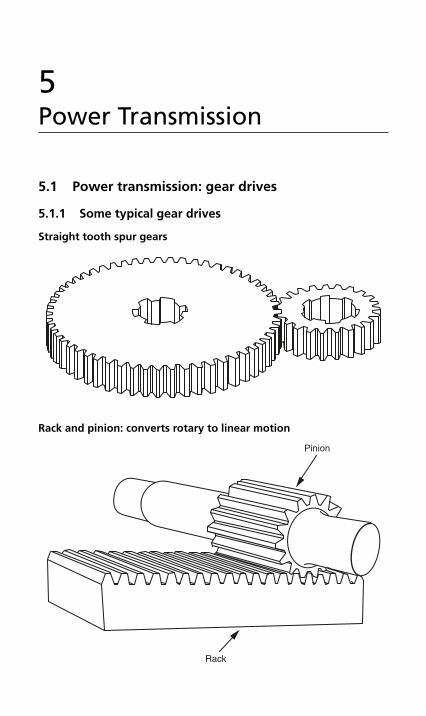
5Power Transmission
5.1 Power transmission: gear drives
5.1.1 Some typical gear drives
Straight tooth spur gears
Rack and pinion: converts rotary to linear motion
Pinion
Rack
H6508-Ch05.1.qxd 9/12/05 4:50 PM Page 351

Single-helical tooth spur gears
Double-helical tooth spur gears
352 Mechanical Engineer’s Pocket Book
H6508-Ch05.1.qxd 9/12/05 4:50 PM Page 352

Straight tooth bevel gears
Worm and worm wheel
Power Transmission 353
H6508-Ch05.1.qxd 9/12/05 4:50 PM Page 353
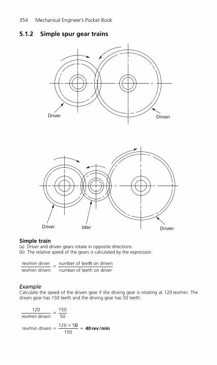
5.1.2 Simple spur gear trains
Simple train(a) Driver and driven gears rotate in opposite directions.(b) The relative speed of the gears is calculated by the expression:
ExampleCalculate the speed of the driven gear if the driving gear is rotating at 120 rev/min. Thedriven gear has 150 teeth and the driving gear has 50 teeth:
120rev/min driven
15050
rev/min driven120 5
�
�� 00
150� 40 rev/min
rev/min driverrev/min driven
number of teet�
hh on drivennumber of teeth on driver
354 Mechanical Engineer’s Pocket Book
Driver Idler Driven
DrivenDriver
H6508-Ch05.1.qxd 9/12/05 4:50 PM Page 354
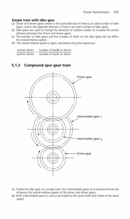
Simple train with idler gear(a) Driver and driven gears rotate in the same direction if there is an odd number of idler
gears, and in the opposite direction if there is an even number of idler gears.(b) Idler gears are used to change the direction of rotation and/or to increase the centre
distance between the driver and driven gears.(c) The number of idler gears and the number of teeth on the idler gears do not affect
the overall relative speed.(d) The overall relative speed is again calculated using the expression:
5.1.3 Compound spur gear train
(a) Unlike the idler gear of a simple train, the intermediate gears of a compound train doinfluence the overall relative speeds of the driver and driven gears.
(b) Both intermediate gears (I1 and I2) are keyed to the same shaft and rotate at the samespeed.
rev/min driverrev/min driven
number of teet�
hh on drivennumber of teeth on driver
Power Transmission 355
Driven gear
Driver gear
Intermediate gear I1
Intermediate gear I2
H6508-Ch05.1.qxd 9/12/05 4:50 PM Page 355

(c) Driver and driven gears rotate in the same direction. To reverse the direction of rota-tion an idler gear has to be inserted either between the driver gear and I1 or betweenI2 and the driven gear.
(d) The overall relative speed can be calculated using the expression:
ExampleCalculate the speed of the driven gear given that: the driver rotates at 600 rev/min andhas 30 teeth; I1 has 60 teeth; I2 has 40 teeth; and the driven gear has 80 teeth:
but speed of driver � 600 rev/min
Therefore:
5.1.4 The involute curve
600 41
60
rev/minrev/min driven
Speed driven
�
�00 14
�
� 150 rev/min
rev/min driverrev/min driven
60 8040
41
��
��
30
rev/min driverrev/min driven
number of teet�
hh on
number of teeth on drivernumber of1I �
teeth on drivennumber of teeth on 2I
356 Mechanical Engineer’s Pocket Book
C
Involutecurve
A
O
Base circle
B
Cord
T (point of tangency)
H6508-Ch05.1.qxd 9/12/05 4:50 PM Page 356
The involute curve is used for the teeth of the majority of industrially produced spur gears.The figure shows that the involute curve can be produced by unwinding an imaginarytaut cord BTC from around a base circle, centre O, commencing with the end of the cordat A. The curve AC which is produced this way has an involute form.
The curvature of AC depends on the radius of the base circle. As the radius of the basecircle increases, the curvature of the involute decreases. For a base circle of infinite radius,the line AC ceases to be a curve and becomes a straight line. Thus a rack gear has teethwith straight sides, since a rack can be considered as part of the circumference of a gearof infinite radius. That is, a rack with straight sided teeth will always mesh satisfactorilywith a spur gear of involute form.
The advantages of the involute form for spur gear teeth are as follows:
(a) Involute form teeth produce smooth running gears capable of transmitting heavyloads at a constant velocity.
(b) Mating teeth of involute form make mainly rolling contact between their flanks asthey move in and out of mesh. Since sliding contact is minimized, scuffing and wearof the flanks of the teeth is also minimized.
(c) Due to the relationship between the involute form and the straight sided rack form, gear teeth can be rapidly and accurately generated using rack type cutters witheasily produced straight flank cutting teeth. This has obvious advantages for toolingcosts.
5.1.5 Basic gear tooth geometry
In order to develop a practical gear tooth form from the basic involute form considered inSection 5.1.4, it is necessary to consider two further geometrical relationships:
(a) A tangent to an involute curve, at any point, is always perpendicular to a tangent tothe base circle drawn from the same point. Reference to Section 5.1.4 shows that theline CT is tangential to the base circle and that such a tangent is perpendicular to atangent drawn to the involute curve at C. It will be shown that the tangent CT is alsothe line of action of a gear teeth.
(b) The length of the line CT is also equal to the length of the arc AT.
Consider two circles touching at the point P as shown overleaf. The point P is called thepitch point, and the circles are called reference circles. If the reference circles were frictiondiscs they would drive each other at the required velocity ratio depending on their relativediameters. However, gears which depended solely on friction to transmit power would bevery limited. In practice they are provided with interlocking teeth to prevent slip. If invo-lute form teeth are used then two additional circles have to be added to the figure asshown. These additional circles are the base circles from which the involutes are drawn(Section 5.1.4). Involutes are now drawn from these base circles so that they touch on theline of action. This line of action is the common tangent to the base circles and is anextension of the line CT (Section 5.1.4).
Power Transmission 357
H6508-Ch05.1.qxd 9/12/05 4:50 PM Page 357
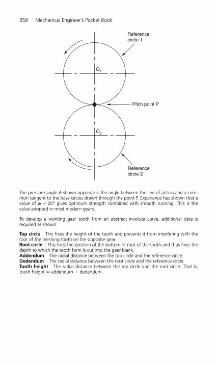
The pressure angle � shown opposite is the angle between the line of action and a com-mon tangent to the base circles drawn through the point P. Experience has shown that avalue of � � 20° gives optimum strength combined with smooth running. This is thevalue adopted in most modern gears.
To develop a working gear tooth from an abstract involute curve, additional data isrequired as shown:
Top circle This fixes the height of the tooth and prevents it from interfering with theroot of the meshing tooth on the opposite gear.Root circle This fixes the position of the bottom or root of the tooth and thus fixes thedepth to which the tooth form is cut into the gear blank.Addendum The radial distance between the top circle and the reference circle.Dedendum The radial distance between the root circle and the reference circle.Tooth height The radial distance between the top circle and the root circle. That is,tooth height � addendum � dedendum.
358 Mechanical Engineer’s Pocket Book
Referencecircle 1
Referencecircle 2
Pitch point P
O1
O2
H6508-Ch05.1.qxd 9/12/05 4:50 PM Page 358
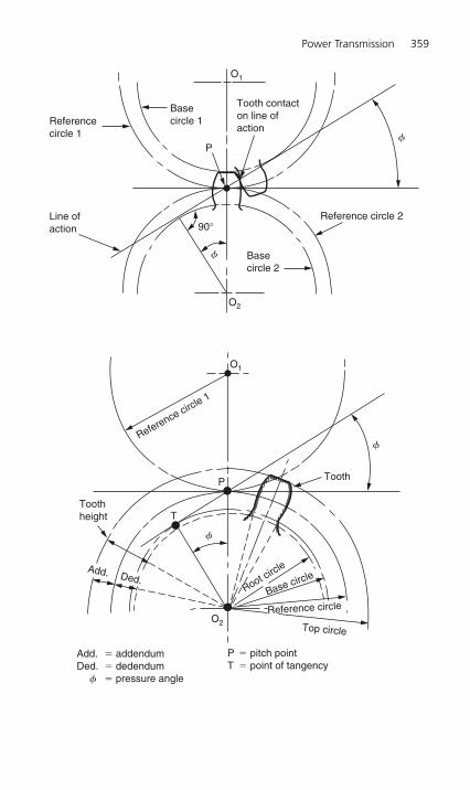
Power Transmission 359
O1
O2
O2
O1
Tooth contacton line ofaction
Basecircle 1
Basecircle 2
P
P
T
Referencecircle 1
Line ofaction 90°
f
f
f
f
Reference circle 2
Reference circle 1
Tooth
Toothheight
Add. Ded.Root circle
Base circle
Reference circle
Top circle
Add. � addendumDed. � dedendum f � pressure angle
P � pitch pointT � point of tangency
H6508-Ch05.1.qxd 9/12/05 4:50 PM Page 359

Note that the involute gear tooth form is an involute from the base circle to the top circle,but has a radial form from the root circle to the base circle as shown in the following figure.
Rack formThe involute relationships applied to the rack tooth are as shown. The rack is the basis forany system of gearing and is, therefore, the starting point from which to build up a seriesof gears.
As shown, the theoretical rack has straight flanks and sharply defined corners. For prac-tical reasons this tooth form is modified by radiusing the tip and replacing the sharp corners at the root with fillets.
360 Mechanical Engineer’s Pocket Book
Add.
Ded.
Involute formfrom base circleto top circle
Radial form frombase circle toroot circle
O2
Add.
Tooth height
Theoretical rack tooth form
Ded.
fP
Reference line2f
H6508-Ch05.1.qxd 9/12/05 4:50 PM Page 360
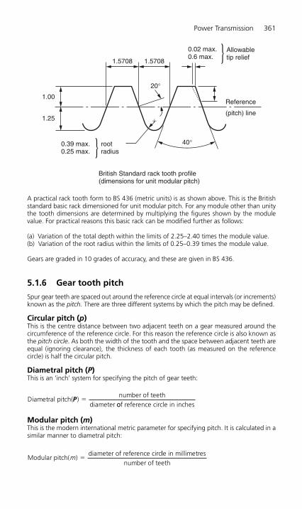
A practical rack tooth form to BS 436 (metric units) is as shown above. This is the Britishstandard basic rack dimensioned for unit modular pitch. For any module other than unitythe tooth dimensions are determined by multiplying the figures shown by the modulevalue. For practical reasons this basic rack can be modified further as follows:
(a) Variation of the total depth within the limits of 2.25–2.40 times the module value.(b) Variation of the root radius within the limits of 0.25–0.39 times the module value.
Gears are graded in 10 grades of accuracy, and these are given in BS 436.
5.1.6 Gear tooth pitch
Spur gear teeth are spaced out around the reference circle at equal intervals (or increments)known as the pitch. There are three different systems by which the pitch may be defined.
Circular pitch (p)This is the centre distance between two adjacent teeth on a gear measured around thecircumference of the reference circle. For this reason the reference circle is also known asthe pitch circle. As both the width of the tooth and the space between adjacent teeth areequal (ignoring clearance), the thickness of each tooth (as measured on the reference circle) is half the circular pitch.
Diametral pitch (P)This is an ‘inch’ system for specifying the pitch of gear teeth:
Modular pitch (m)This is the modern international metric parameter for specifying pitch. It is calculated in asimilar manner to diametral pitch:
Modular pitch( )diameter of reference circ
m �lle in millimetres
number of teeth
Diametral pitch( )number of teeth
diameterP �
oof reference circle in inches
1.00
1.25
0.39 max.0.25 max.
rootradius
British Standard rack tooth profile(dimensions for unit modular pitch)
�
Reference
(pitch) line
20°
40°
1.5708 1.5708
0.02 max.0.6 max.
Allowabletip relief
Power Transmission 361
H6508-Ch05.1.qxd 9/12/05 4:50 PM Page 361
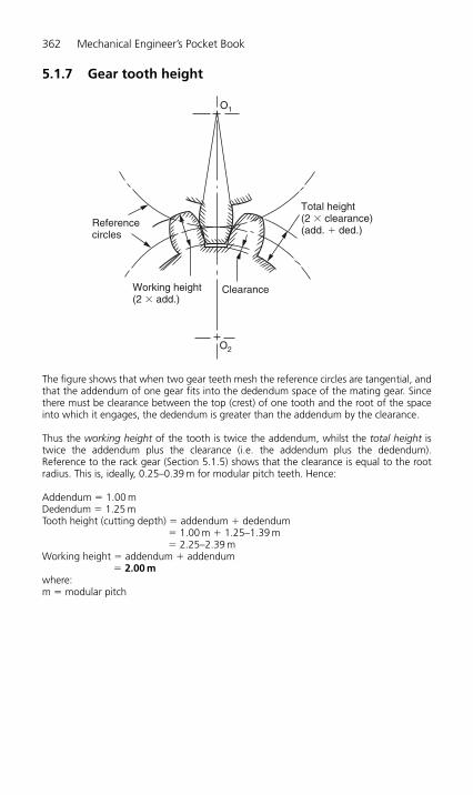
5.1.7 Gear tooth height
The figure shows that when two gear teeth mesh the reference circles are tangential, andthat the addendum of one gear fits into the dedendum space of the mating gear. Sincethere must be clearance between the top (crest) of one tooth and the root of the spaceinto which it engages, the dedendum is greater than the addendum by the clearance.
Thus the working height of the tooth is twice the addendum, whilst the total height istwice the addendum plus the clearance (i.e. the addendum plus the dedendum).Reference to the rack gear (Section 5.1.5) shows that the clearance is equal to the rootradius. This is, ideally, 0.25–0.39 m for modular pitch teeth. Hence:
Addendum � 1.00 mDedendum � 1.25 mTooth height (cutting depth) � addendum � dedendum
� 1.00 m � 1.25–1.39 m� 2.25–2.39 m
Working height � addendum � addendum� 2.00 m
where:m � modular pitch
362 Mechanical Engineer’s Pocket Book
Referencecircles
Working height(2 � add.)
Clearance
O2
O1
Total height(2 � clearance)(add. � ded.)
H6508-Ch05.1.qxd 9/12/05 4:50 PM Page 362

Power Transm
ission363
5.1.8 Standard gear tooth elements (in.)
Normal diametral Normal circular Standard circular Standard Standard Minimum Minimum Total shaving stock pitch pitch tooth thickness addendum work depth clearance* whole depth* on tooth thickness
2.5 1.256637 0.6283 0.4000 0.8000 0.090 0.890 0.0040/0.00503 1.047198 0.5236 0.3333 0.6666 0.083 0.750 0.0040/0.00503.5 0.897598 0.4488 0.2857 0.5714 0.074 0.645 0.0040/0.00504 0.785398 0.3927 0.2500 0.5000 0.068 0.568 0.0035/0.00454.5 0.698132 0.3491 0.2222 0.4444 0.060 0.504 0.0035/0.00455 0.628319 0.3142 0.2000 0.4000 0.056 0.456 0.0035/0.00456 0.523599 0.2618 0.1667 0.3334 0.050 0.383 0.0030/0.00407 0.448799 0.2244 0.1429 0.2858 0.044 0.330 0.0030/0.00408 0.392699 0.1963 0.1250 0.2500 0.040 0.290 0.0030/0.00409 0.349066 0.1745 0.1111 0.2222 0.038 0.260 0.0025/0.0035
10 0.314159 0.1571 0.1000 0.2000 0.035 0.235 0.0025/0.003511 0.285599 0.1428 0.0909 0.1818 0.032 0.214 0.0020/0.003012 0.261799 0.1309 0.0833 0.1666 0.030 0.197 0.0020/0.003014 0.224399 0.1122 0.0714 0.1428 0.026 0.169 0.0020/0.003016 0.196350 0.0982 0.0625 0.1250 0.023 0.148 0.0015/0.002518 0.174533 0.0873 0.0556 0.1112 0.021 0.132 0.0015/0.0025
* Based on standard tip radius on preshaving hobs and shaper cutters. Increase whole depth by approximately 0.005–0.010 in. for crown shaving.
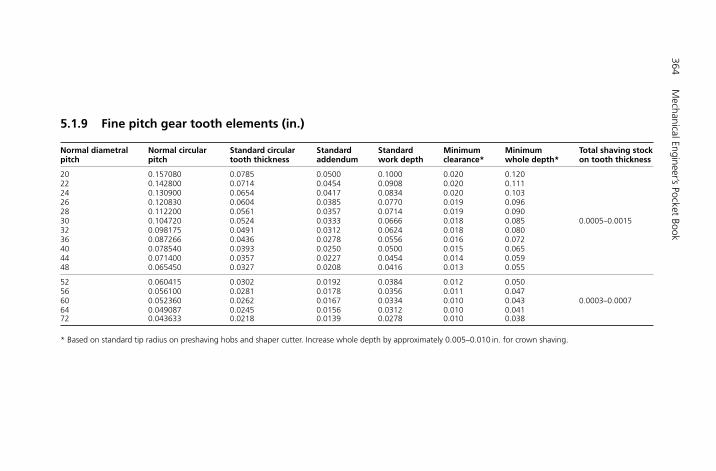
364M
echanical Engineer’s Pocket Book
5.1.9 Fine pitch gear tooth elements (in.)
Normal diametral Normal circular Standard circular Standard Standard Minimum Minimum Total shaving stock pitch pitch tooth thickness addendum work depth clearance* whole depth* on tooth thickness
20 0.157080 0.0785 0.0500 0.1000 0.020 0.12022 0.142800 0.0714 0.0454 0.0908 0.020 0.11124 0.130900 0.0654 0.0417 0.0834 0.020 0.10326 0.120830 0.0604 0.0385 0.0770 0.019 0.09628 0.112200 0.0561 0.0357 0.0714 0.019 0.09030 0.104720 0.0524 0.0333 0.0666 0.018 0.085 0.0005–0.001532 0.098175 0.0491 0.0312 0.0624 0.018 0.08036 0.087266 0.0436 0.0278 0.0556 0.016 0.07240 0.078540 0.0393 0.0250 0.0500 0.015 0.06544 0.071400 0.0357 0.0227 0.0454 0.014 0.05948 0.065450 0.0327 0.0208 0.0416 0.013 0.055
52 0.060415 0.0302 0.0192 0.0384 0.012 0.05056 0.056100 0.0281 0.0178 0.0356 0.011 0.04760 0.052360 0.0262 0.0167 0.0334 0.010 0.043 0.0003–0.000764 0.049087 0.0245 0.0156 0.0312 0.010 0.04172 0.043633 0.0218 0.0139 0.0278 0.010 0.038
* Based on standard tip radius on preshaving hobs and shaper cutter. Increase whole depth by approximately 0.005–0.010 in. for crown shaving.

Power Transm
ission365
5.1.10 Standard stub gear tooth elements (in.)
Normal diametral Normal circular Standard circular Standard Standard Minimum Minimum Total shaving stock pitch pitch tooth thickness addendum work depth clearance* whole depth* on tooth thickness
3/4 1.047198 0.5236 0.2500 0.5000 0.083 0.583 0.0040/0.00504/5 0.785398 0.3927 0.2000 0.4000 0.068 0.468 0.0035/0.00455/7 0.628319 0.3142 0.1429 0.2858 0.056 0.342 0.0035/0.00456/8 0.523599 0.2618 0.1250 0.2500 0.050 0.300 0.0030/0.00407/9 0.448799 0.2244 0.1111 0.2222 0.044 0.266 0.0030/0.00408/10 0.392699 0.1963 0.1000 0.2000 0.040 0.240 0.0030/0.00409/11 0.349066 0.1745 0.0909 0.1818 0.038 0.220 0.0025/0.0035
10/12 0.314159 0.1571 0.0833 0.1666 0.035 0.202 0.0025/0.003512/14 0.261799 0.1309 0.0714 0.1428 0.030 0.173 0.0020/0.003014/18 0.224399 0.1122 0.0556 0.1112 0.026 0.137 0.0020/0.003016/21 0.196350 0.0982 0.0476 0.0952 0.023 0.118 0.0015/0.002518/24 0.174533 0.0873 0.0417 0.0834 0.021 0.104 0.0015/0.002520/26 0.157080 0.0785 0.0385 0.0770 0.020 0.097 0.0010/0.001522/29 0.142800 0.0714 0.0345 0.0690 0.020 0.089 0.0010/0.001524/32 0.130900 0.0654 0.0313 0.0626 0.020 0.083 0.0010/0.001526/35 0.120830 0.0604 0.0286 0.0572 0.019 0.076 0.0010/0.001528/37 0.112200 0.0561 0.0270 0.0540 0.019 0.073 0.0010/0.001530/40 0.104720 0.0524 0.0250 0.0500 0.018 0.068 0.0010/0.001532/42 0.098175 0.0491 0.0238 0.0476 0.018 0.066 0.0010/0.001534/45 0.092400 0.0462 0.0222 0.0444 0.017 0.061 0.0010/0.001536/48 0.087266 0.0436 0.0208 0.0416 0.016 0.058 0.0010/0.001538/50 0.082673 0.0413 0.0200 0.0400 0.016 0.056 0.0010/0.001540/54 0.078540 0.0393 0.0185 0.0370 0.015 0.052 0.0010/0.0015
* Based on standard tip radius on preshaving hobs and shaper cutters. Increase whole depth by approximately 0.005–0.010 in. for crown shaving.
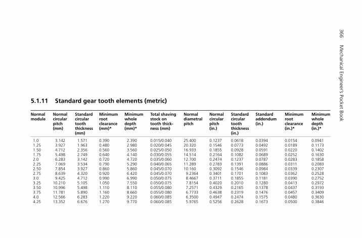
366M
echanical Engineer’s Pocket Book
5.1.11 Standard gear tooth elements (metric)
Normal Normal Standard Minimum Minimum Total shaving Normal Normal Standard Standard Minimum Minimum module circular circular root whole stock on diametral circular circular addendum root whole
pitch tooth clearance depth tooth thick- pitch pitch tooth (in.) clearance depth (mm) thickness (mm)* (mm)* ness (mm) (in.) thickness (in.)* (in.)*
(mm) (in.)
1.0 3.142 1.571 0.390 2.390 0.015/0.040 25.400 0.1237 0.0618 0.0394 0.0154 0.09411.25 3.927 1.963 0.480 2.980 0.020/0.045 20.320 0.1546 0.0773 0.0492 0.0189 0.11731.50 4.712 2.356 0.560 3.560 0.025/0.050 16.933 0.1855 0.0928 0.0591 0.0220 0.14021.75 5.498 2.749 0.640 4.140 0.030/0.055 14.514 0.2164 0.1082 0.0689 0.0252 0.16302.0 6.283 3.142 0.720 4.720 0.035/0.060 12.700 0.2474 0.1237 0.0787 0.0283 0.18582.25 7.069 3.534 0.790 5.290 0.040/0.065 11.289 0.2783 0.1391 0.0886 0.0311 0.20832.50 7.854 3.927 0.860 5.860 0.045/0.070 10.160 0.3092 0.1546 0.0984 0.0339 0.23072.75 8.639 4.320 0.920 6.420 0.045/0.070 9.2364 0.3401 0.1701 0.1083 0.0362 0.25283.0 9.425 4.712 0.990 6.990 0.050/0.075 8.4667 0.3711 0.1855 0.1181 0.0390 0.27523.25 10.210 5.105 1.050 7.550 0.050/0.075 7.8154 0.4020 0.2010 0.1280 0.0413 0.29723.50 10.996 5.498 1.110 8.110 0.055/0.080 7.2571 0.4329 0.2165 0.1378 0.0437 0.31933.75 11.781 5.890 1.160 8.660 0.055/0.080 6.7733 0.4638 0.2319 0.1476 0.0457 0.34094.0 12.566 6.283 1.220 9.220 0.060/0.085 6.3500 0.4947 0.2474 0.1575 0.0480 0.36304.25 13.352 6.676 1.270 9.770 0.060/0.085 5.9765 0.5256 0.2628 0.1673 0.0500 0.3846
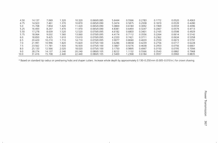
Power Transm
ission367
4.50 14.137 7.069 1.320 10.320 0.060/0.085 5.6444 0.5566 0.2783 0.1772 0.0520 0.40634.75 14.923 7.461 1.370 10.870 0.065/0.090 5.3474 0.5875 0.2938 0.1870 0.0539 0.42805.0 15.708 7.854 1.420 11.420 0.065/0.090 5.0800 0.6184 0.3092 0.1969 0.0559 0.44965.25 16.493 8.247 1.470 11.970 0.065/0.090 4.8381 0.6493 0.3247 0.2067 0.0579 0.47135.50 17.278 8.639 1.520 12.520 0.070/0.095 4.6182 0.6803 0.3401 0.2165 0.0598 0.49295.75 18.064 9.032 1.560 13.060 0.070/0.095 4.4174 0.7112 0.3556 0.2264 0.0614 0.51426.0 18.850 9.425 1.610 13.610 0.070/0.095 4.2333 0.7421 0.3711 0.2362 0.0634 0.53586.5 20.420 10.210 1.710 14.710 0.070/0.095 3.9077 0.8040 0.4020 0.2559 0.0673 0.57917.0 21.991 10.996 1.820 15.820 0.075/0.100 3.6286 0.8658 0.4239 0.2756 0.0717 0.62287.5 23.562 11.781 1.920 16.920 0.075/0.100 3.3867 0.9276 0.4638 0.2953 0.0756 0.66618.0 25.133 12.566 2.020 18.020 0.075/0.100 3.1750 0.9895 0.4947 0.3150 0.0795 0.70949.0 28.274 14.137 2.240 20.240 0.080/0.105 2.8222 1.1132 0.5566 0.3543 0.0882 0.7968
10.0 31.416 15.708 2.440 22.440 0.080/0.105 2.5400 1.2368 0.6184 0.3937 0.0960 0.8835
* Based on standard tip radius on preshaving hobs and shaper cutters. Increase whole depth by approximately 0.130–0.250 mm (0.005–0.010 in.) for crown shaving.
H6508-Ch05.1.qxd 9/12/05 4:50 PM Page 367

368 Mechanical Engineer’s Pocket Book
5.1.12 Letter symbols for gear dimensions and calculations
a addendumb dedendumB backlashBn normal circular backlashc clearanceC centre distanced diameter of measuring pin or ballD pitch diameterDb base diameterDc contact diameterDf form diameterDF fillet diameterDi minor diameter (internal gears)Dm diameter of circle through centre of measuring pins or ballsDMe measurement over pins or balls (external)DMi measurement between pins or balls (internal)Do outside diameter (O/D)Dr rolling or operating pitch diameterDR root diameterDs shaved diameterF face widthhk working depthht whole depthL leadLA total length of line of actionm module (metric system)mF face contact ratio (helical overlap)mn normal modulemp involute contact ratio (involute overlap)mt transverse moduleN number of teeth in gear (NG) or pinion (Np)p circular pitchpb base pitchpn normal circular pitchpt transverse circular pitchpx axial pitchP diametral pitchPn normal diametral pitchPt transverse diametral pitchSAP start of active profileS circular tooth spaceSRP start of radius profileSn normal circular tooth spaceSt transverse circular tooth spacet circular tooth thickness (tn, tt, etc.)tc chordal tooth thickness (tnc, ttc, etc.)Z length of contact
Angles� pressure angle�m pressure angle to centre of measuring pin or ball�n normal pressure angle�r operating pressure angle (�nr, �tr, etc.)�t transverse pressure angle
H6508-Ch05.1.qxd 9/12/05 4:50 PM Page 368
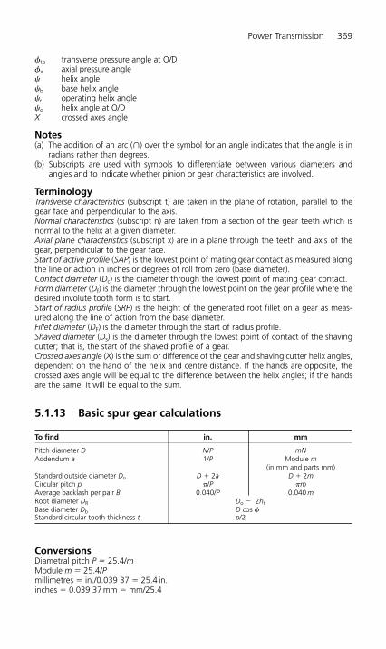
Power Transmission 369
�to transverse pressure angle at O/D�x axial pressure angle� helix angle�b base helix angle�r operating helix angle�o helix angle at O/DX crossed axes angle
Notes(a) The addition of an arc (�) over the symbol for an angle indicates that the angle is in
radians rather than degrees.(b) Subscripts are used with symbols to differentiate between various diameters and
angles and to indicate whether pinion or gear characteristics are involved.
TerminologyTransverse characteristics (subscript t) are taken in the plane of rotation, parallel to thegear face and perpendicular to the axis.Normal characteristics (subscript n) are taken from a section of the gear teeth which isnormal to the helix at a given diameter.Axial plane characteristics (subscript x) are in a plane through the teeth and axis of thegear, perpendicular to the gear face.Start of active profile (SAP) is the lowest point of mating gear contact as measured alongthe line or action in inches or degrees of roll from zero (base diameter).Contact diameter (Dc) is the diameter through the lowest point of mating gear contact.Form diameter (Df) is the diameter through the lowest point on the gear profile where thedesired involute tooth form is to start.Start of radius profile (SRP) is the height of the generated root fillet on a gear as meas-ured along the line of action from the base diameter.Fillet diameter (DF) is the diameter through the start of radius profile.Shaved diameter (Ds) is the diameter through the lowest point of contact of the shavingcutter; that is, the start of the shaved profile of a gear.Crossed axes angle (X) is the sum or difference of the gear and shaving cutter helix angles,dependent on the hand of the helix and centre distance. If the hands are opposite, thecrossed axes angle will be equal to the difference between the helix angles; if the handsare the same, it will be equal to the sum.
5.1.13 Basic spur gear calculations
To find in. mm
Pitch diameter D N/P mNAddendum a 1/P Module m
(in mm and parts mm)Standard outside diameter Do D � 2a D � 2mCircular pitch p �/P �mAverage backlash per pair B 0.040/P 0.040 mRoot diameter DR Do � 2htBase diameter Db D cos �Standard circular tooth thickness t p/2
ConversionsDiametral pitch P � 25.4/mModule m � 25.4/Pmillimetres � in./0.039 37 � 25.4 in.inches � 0.039 37 mm � mm/25.4
H6508-Ch05.1.qxd 9/12/05 4:50 PM Page 369

370 Mechanical Engineer’s Pocket Book
5.1.14 Basic helical gear equations
Transverse diametral pitch Pt � Pn cos �Pitch diameter D � N/PtAddendum a standard � 1/PnOutside diameter Do � D � 2aTransverse pressure angle �t: tan �t � tan �n/cos �Base diameter Db � D cos �tLead L � �D cot � � �D/tan �Normal circular pitch pn � �/PnStandard normal circular tooth thickness tn � pn/2Axial pitch px � �/Pn sin � � pn/sin � � L/NTransverse circular pitch pt � �/Pt � pn/cos �
5.1.15 Miscellaneous gear equations
1. Helix angle �, when given centre distance is standard:
2. Operating pitch diameter (pinion), with non-standard centre distance C:
3. Operating pressure angle �rt, with non-standard centre distance C:
4. Normal diametral pitch:
Pn � Pt sec �
5. Helix angle �:
At any diameter D2:
6. Transverse circular pitch pt2 at any diameter D2:
pD
Nt22�
p
tan 21
1
cc
�D
D2 tan
cos
sin
n
n
c
cp
�
�
NDP
NP L
cos2rt
bp bG
f ��D D
C
DCN
N Nrpp
p G
2�
�
cos2p G
n
c ��N N
p C
H6508-Ch05.1.qxd 9/12/05 4:50 PM Page 370

7. Involute function of pressure angle (function tables are available):
inv � � tan � � �
8. Normal pressure angle (�n):
tan �n � tan �t cos �
9. Transverse pressure angle �t at any diameter D2:
10. Base helix angle �b:
11. Base pitch:
5.1.16 Straight bevel gear nomenclature
pD
Npb
b cos� �p
f
coscos cos
cos
sin
sin
sin
bn
t
n
t
b
cc f
f
f
f
c
� �
��
�
sin cos
tan tan cos
n
b t
c f
c c f
cos t2b
2
f �D
D
Power Transmission 371
Face width
Back angle
Backconeangle
Pitch diameter
Outside diameter
Gear
Back
con
edi
stan
ce
PinionUniformclearance
Shaftangle
Dedendumangle
Addendumangle
Pitch apex(datum)
Cone distance
Pitchangle
Pitch apex to back
Pitch apex to crown Crown to back
Rootangle
Frontangle
H6508-Ch05.1.qxd 9/12/05 4:50 PM Page 371
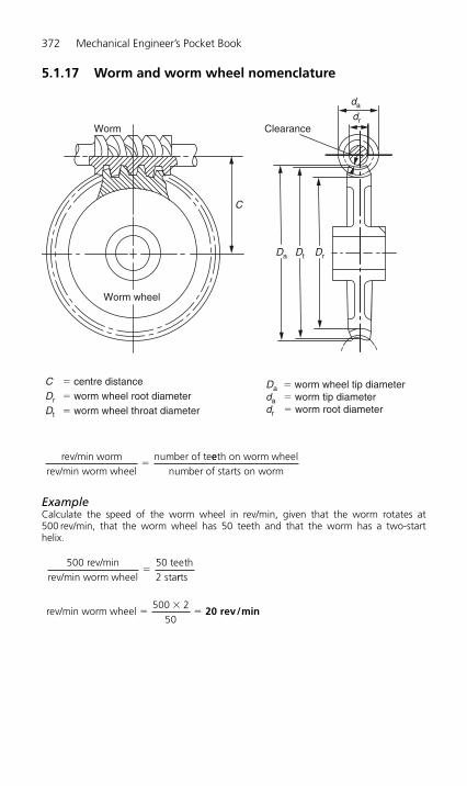
372 Mechanical Engineer’s Pocket Book
5.1.17 Worm and worm wheel nomenclature
ExampleCalculate the speed of the worm wheel in rev/min, given that the worm rotates at500 rev/min, that the worm wheel has 50 teeth and that the worm has a two-start helix.
500 rev/minrev/min worm wheel
50 teeth2 sta
�rrts
rev/min worm wheel500 2
50�
�� 20 rev/min
rev/min wormrev/min worm wheel
number of te�
eeth on worm wheelnumber of starts on worm
Worm Clearance
da
dr
Da Dt Dr
C
Worm wheel
C � centre distanceDr � worm wheel root diameterDt � worm wheel throat diameter
Da � worm wheel tip diameterda � worm tip diameterdr � worm root diameter
H6508-Ch05.1.qxd 9/12/05 4:50 PM Page 372
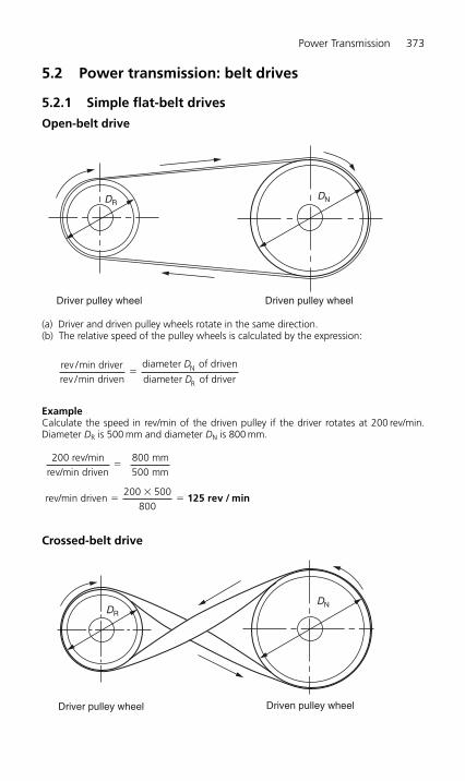
Power Transmission 373
5.2 Power transmission: belt drives
5.2.1 Simple flat-belt drives
Open-belt drive
(a) Driver and driven pulley wheels rotate in the same direction.(b) The relative speed of the pulley wheels is calculated by the expression:
ExampleCalculate the speed in rev/min of the driven pulley if the driver rotates at 200 rev/min.Diameter DR is 500 mm and diameter DN is 800 mm.
Crossed-belt drive
DNDR
Driver pulley wheel Driven pulley wheel
rev/min driven200 500
��
�800
125 rev / min
200500
rev/minrev/min driven
800 mmmm
�
rev /min driverrev /min driven
diameter ofN�D driven
diameter of driverRD
Driver pulley wheel Driven pulley wheel
DNDR
H6508-Ch05.2.qxd 9/12/05 4:49 PM Page 373
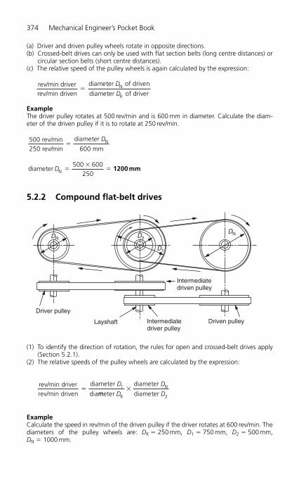
(a) Driver and driven pulley wheels rotate in opposite directions.(b) Crossed-belt drives can only be used with flat section belts (long centre distances) or
circular section belts (short centre distances).(c) The relative speed of the pulley wheels is again calculated by the expression:
ExampleThe driver pulley rotates at 500 rev/min and is 600 mm in diameter. Calculate the diam-eter of the driven pulley if it is to rotate at 250 rev/min.
5.2.2 Compound flat-belt drives
(1) To identify the direction of rotation, the rules for open and crossed-belt drives apply(Section 5.2.1).
(2) The relative speeds of the pulley wheels are calculated by the expression:
ExampleCalculate the speed in rev/min of the driven pulley if the driver rotates at 600 rev/min. Thediameters of the pulley wheels are: DR � 250 mm, D1 � 750 mm, D2 � 500 mm,DN � 1000 mm.
rev/min driverrev/min driven
diameter
dia1�
D
mmeter
diameter
diameterR
N
2D
D
D�
Driver pulley
Layshaft Intermediatedriver pulley
Driven pulley
Intermediatedriven pulley
DN
D1
D2DR
diameter500 600
N ��
�D250
1200 mm
500250 600
rev/minrev/min
diameter
mmN�
D
rev/min driverrev/min driven
diameter ofN�D driven
diameter of driverRD
374 Mechanical Engineer’s Pocket Book
H6508-Ch05.2.qxd 9/12/05 4:49 PM Page 374
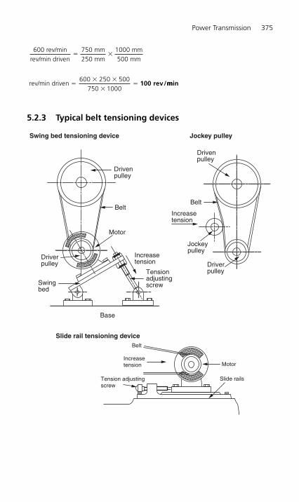
5.2.3 Typical belt tensioning devices
Belt
Increasetension
Tension adjustingscrew
Motor
Slide rails
Slide rail tensioning device
Drivenpulley
Belt
Motor
Driverpulley
Increasetension
Tensionadjustingscrew
Drivenpulley
Belt
Increasetension
Jockeypulley
Driverpulley
Swingbed
Base
Swing bed tensioning device Jockey pulley
rev/min driven600 250 500
1000�
� �
��
750100 rev/mmin
600250
rev/minrev/min driven
750 mmmm
1000� �
mmmm500
Power Transmission 375
H6508-Ch05.2.qxd 9/12/05 4:49 PM Page 375

376 Mechanical Engineer’s Pocket Book
Application FO®-Z ULTRAFLEX® MULTIFLEX®
heavy-duty narrow-section classical-section cogged raw wrapped V-belts wrapped V-beltsedge V-belts
Construction machinery Soil-compacting Concrete mixers Impact crushersequipment
Mining Underground Underground application application
Office equipment Paper shreddersSpeed adjustable gear units Interlocking pulleys
Printing equipment Rotary pressesElectric power generation Emergency
back-up systemsElectric-operated tools Oscillating
grindersConveying Conveyor drives Bucket conveyors
Industrial drives Power Power Power transmissions transmissions transmissions
Large domestic appliancesSmall domestic appliances MixersWoodworking machinery Planing equipment Reciprocating
sawsRubber and plastics processing Extruders
Automotive sector Auxiliary unitsCompressors Piston
compressorsAgricultural equipment Blowers Spreaders Beet liftersMotorcycles
Paper-making machinery Drying cylindersPumps Radial-flow pumpsLawn care and cleaning equipmentTextile machinery Cylindrical dryers
Ventilators Axial-flow blowersInternal combustion engines Auxiliary unitsMetalworking machinery LathesCrushing/grinding machinery
5.2.4 Typical V-belt and synchronous-belt drive applications
H6508-Ch05.2.qxd 9/12/05 4:49 PM Page 376
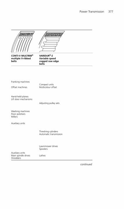
Power Transmission 377
CONTI-V MULTIRIB® VARIDUR®-Z multiple V-ribbed Variable speed belts cogged raw edge
belts
Franking machinesCompact units
Offset machines Multicolour offset
Hand-held planesLift door mechanisms
Adjusting pulley sets
Washing machinesFloor polishersMillers
Auxiliary units
Threshing cylindersAutomatic transmission
Lawnmower drivesSpoolers
Auxiliary unitsMain spindle drives LathesShredders
continued
H6508-Ch05.2.qxd 9/12/05 4:49 PM Page 377

378 Mechanical Engineer’s Pocket Book
Section 5.2.4 (continued )
Application VARIFLEX®-Z variable speed cogged belts
Office equipmentData processingSpeed adjustable gear units
Printing equipment Letterpress printing machines
Electric-operated toolsFilm projectorsConveying
Industrial drives Adjusting pulley setsSmall domestic appliancesWoodworking machinery
Automotive sectorSewing machines
Lawn care and cleaning equipmentRoboticsTextile machinery
VentilatorsInternal combustion enginesPackaging machines
Metalworking machinery
H6508-Ch05.2.qxd 9/12/05 4:49 PM Page 378

Power Transmission 379
SYNCHROBELT® and SYNCHROBELT®
SYNCHROFORCE® synchronous high torque drive beltsdrive belts
Photocopiers TypewritersHard-copy printers Plotters
Rotary presses
Hand-held planes Belt grindersReel drivesLift control systems
Reduction gears Reduction gearDomestic appliances Turbo-brushersAdhesive bonding equipment
Camshaft drives Camshaft drivesLooper drives
CultivatorsPositioning drives Positioning drivesWeaving machines
Main drivesCamshaft drives Camshaft drives
Counters
Power feed drives
All data is supplied by ContiTech P.T.S. Ltd whose technical publications should be consulted for fullproduct range, applications and technical data. (See Appendix 3 for full details.)Note: CONTICORD® flat belts and CON-FLEX® driving belts, are no longer available.
H6508-Ch05.2.qxd 9/12/05 4:49 PM Page 379

5.2.5 ULTRAFLEX® narrow-section wrapped V-belts
380M
echanical Engineer’s Pocket Book
bw
h h
h w h w
bo bo
bw
d p
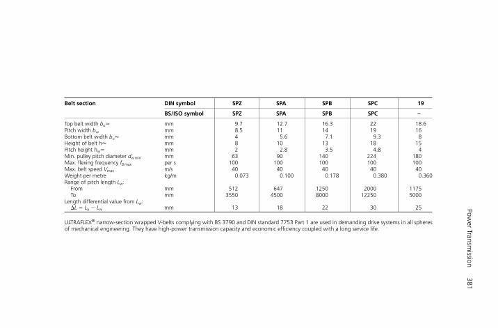
Power Transm
ission381
Belt section DIN symbol SPZ SPA SPB SPC 19
BS/ISO symbol SPZ SPA SPB SPC –
Top belt width bo� mm 9.7 12.7 16.3 22 18.6Pitch width bw mm 8.5 11 14 19 16Bottom belt width bu� mm 4 5.6 7.1 9.3 8Height of belt h� mm 8 10 13 18 15Pitch height hw� mm 2 2.8 3.5 4.8 4Min. pulley pitch diameter dw min mm 63 90 140 224 180Max. flexing frequency fB max per s 100 100 100 100 100Max. belt speed Vmax m/s 40 40 40 40 40Weight per metre kg/m 0.073 0.100 0.178 0.380 0.360Range of pitch length Lw:
From mm 512 647 1250 2000 1175To mm 3550 4500 8000 12250 5000
Length differential value from Lw:�L � La � Lw mm 13 18 22 30 25
ULTRAFLEX® narrow-section wrapped V-belts complying with BS 3790 and DIN standard 7753 Part 1 are used in demanding drive systems in all spheresof mechanical engineering. They have high-power transmission capacity and economic efficiency coupled with a long service life.
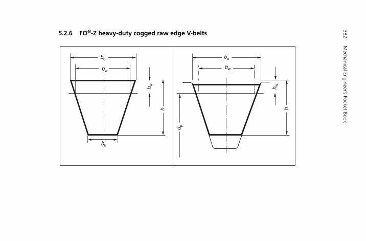
5.2.6 FO®-Z heavy-duty cogged raw edge V-belts
382M
echanical Engineer’s Pocket Book
bw
bu
h h
h w h w
bo bo
bw
d p

Power Transm
ission383
Belt section DIN symbol 5 6 SPZ SPA SPB
BS/ISO symbol – Y SPZ SPA SPB
Top belt width bo� mm 5 6 10 13 16.3Pitch width bw mm 4.2 5.3 8.5 11 14Height of belt h� mm 3 4 8 9 13Pitch height hw� mm 1.3 1.6 2 2.8 3.5Min. pulley pitch diameter dw min mm 16 20 50 63 100Max. flexing frequency fB max per s 120 120 120 120 120Max. belt speed vmax m/s 50 50 50 50 50Weight per metre kg/m 0.015 0.023 0.073 0.100 0.178Range of pitch length Lw:
From mm 171 295 590 590 1250To mm 611 865 3550 3550 3550
Length differential value from Lw:�L � Lw � Li mm 11 15 – – –
FO®-Z heavy-duty cogged V-belts are manufactured in a raw edge type and supplement the proven range of CONTI® V-belts. Theycomply in their dimensions as narrow-section V-belts with DIN standard 7753 Part 1 and BS 3790 and as standard V-belts with DINstandard 2215 and BS 3790.
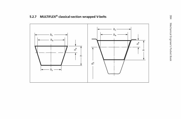
5.2.7 MULTIFLEX® classical-section wrapped V-belts
384M
echanical Engineer’s Pocket Book
bo
bo
bu
b p
bw
bw
h
hh w
h w

Power Transm
ission385
Belt section DIN symbol 8 10 13 17 20 22 25 32 40
BS/ISO – Z A B – C – D Esymbol
Top belt width bo� mm 8 10 13 17 20 22 25 32 40Pitch width bw mm 6.7 8.5 11 14 17 19 21 27 32Bottom belt width bu� mm 4.6 5.9 7.5 9.4 11.4 12.4 14 18.3 22.8Height of belt h� mm 5 6 8 11 12.5 14 16 20 25Pitch height hw� mm 2 2.5 3.3 4.2 4.8 5.7 6.3 8.1 12Min. pulley pitch diameter dw min mm 40 50 80 125 160 200 250 355 500Max. flexing frequency fB max per s 60 60 60 60 60 60 60 60 60Max. belt speed Vmax m/s 30 30 30 30 30 30 30 30 30Weight per metre kg/m 0.040 0.060 0.105 0.170 0.240 0.300 0.430 0.630 0.970Range of pitch length Lw:
From mm 160 375 400 615 900 1150 1400 2080 5080To mm 1250 2500 5000 8763 8000 8000 9000 13460 11280
Length differential value from Li:�L � Lw � Li mm 19 22 30 43 48 52 61 75 82
MULTIFLEX® classical-section wrapped V-belts complying with BS 3790 and DIN standard 2215 are designed for all industrial applications from precision engineering toheavy machine construction.

5.2.8 MULTIBELT banded V-belts
386M
echanical Engineer’s Pocket Book
bobo
d e
h h
e e
Belt dimensions
MULTIBELT banded V-belts form a drive unit combining the advantage of a single-belt with the increasedpower transmission capacity of a multi-groove V-belt set. This drive unit helps solve problems relating to drivesthat formerly involve extensive constructional expenditure.

Power Transm
ission387
Dimensional data
Belt section DIN/ISO symbol 9J SPA 15J 17/B 19 SPC
RMA/ASAE 3V – 5V B/HB – –symbol
Top section width bo� mm 9 12.5 15 16 19 22Height of belt h� mm 11 12 15 13 21 23Lateral rib pitch e mm 10.3 15 17.5 19.05 22 25.5Min. pulley pitch diameter de min mm 67 95.6 180 100 188 265Max. flexing frequency fB max s�1 60 60 60 60 60 60Max. belt speed vmax m/s 30 30 30 30 30 30Weight per rib per metre kg/m 0.115 0.170 0.250 0.240 0.405 0.505Range-outside length La:
From mm 750 1350 1350 1350 2500 2500To mm 2800 2800 5600 5600 5600 5600
Length differential value from La: * – * – – –�L � La � Li mm – – – 62 – –�L � La � Lw mm – 18 – – 25 30
* The reference length La is the designated length for sections 9J and 15J.
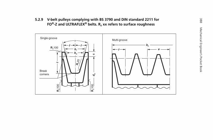
5.2.9 V-belt pulleys complying with BS 3790 and DIN standard 2211 forFO®-Z and ULTRAFLEX® belts. Rz xx refers to surface roughness
388M
echanical Engineer’s Pocket Book
Single-groove
Breakcorners
Multi-groove
Rz1
00
Rz1
00
Rz100
Rz25
bw
b1
b2
c
t
f
f ef
a
dw
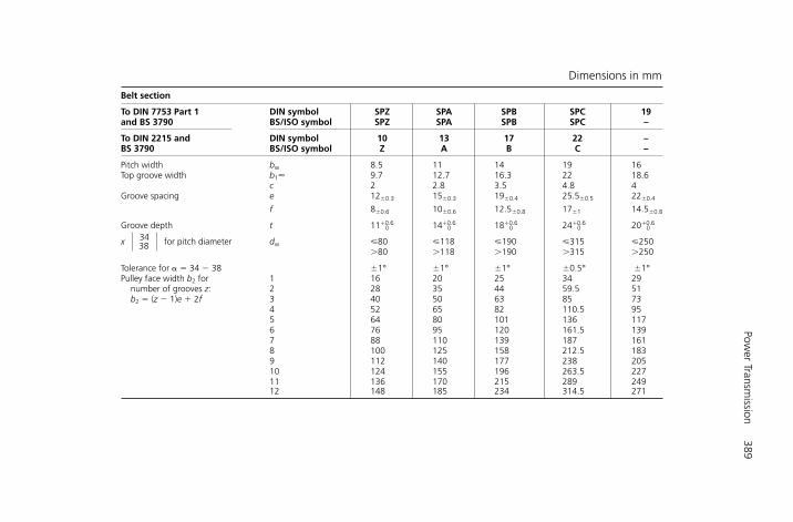
Power Transm
ission389
Belt section
To DIN 7753 Part 1 DIN symbol SPZ SPA SPB SPC 19and BS 3790 BS/ISO symbol SPZ SPA SPB SPC –
To DIN 2215 and DIN symbol 10 13 17 22 –BS 3790 BS/ISO symbol Z A B C –
Pitch width bw 8.5 11 14 19 16Top groove width b1� 9.7 12.7 16.3 22 18.6
c 2 2.8 3.5 4.8 4Groove spacing e 12�0.3 15�0.3 19�0.4 25.5�0.5 22�0.4
f 8�0.6 10�0.6 12.5�0.8 17�1 14.5�0.8
Groove depth t 11�00.6 14�
00.6 18�
00.6 24�
00.6 20�
00.6
x 34 for pitch diameter dw �80 �118 �190 �315 �25038�80 �118 �190 �315 �250
Tolerance for � 34 � 38 �1° �1° �1° �0.5° �1°Pulley face width b2 for 1 16 20 25 34 29
number of grooves z: 2 28 35 44 59.5 51b2 � (z � 1)e � 2f 3 40 50 63 85 73
4 52 65 82 110.5 955 64 80 101 136 1176 76 95 120 161.5 1397 88 110 139 187 1618 100 125 158 212.5 1839 112 140 177 238 20510 124 155 196 263.5 22711 136 170 215 289 24912 148 185 234 314.5 271
Dimensions in mm
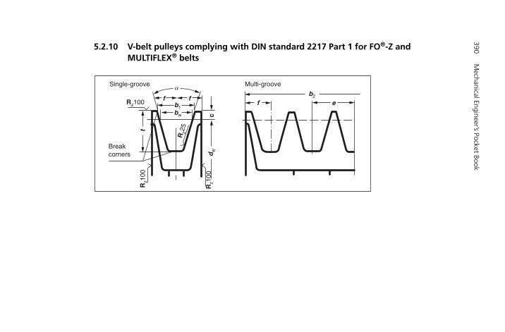
5.2.10 V-belt pulleys complying with DIN standard 2217 Part 1 for FO®-Z and MULTIFLEX® belts
390M
echanical Engineer’s Pocket Book
Multi-groove
Breakcorners
Rz25
dw
Single-groove
Rz100
Rz1
00
Rz1
00
ff e
f
cbw
b1
b2
a
t
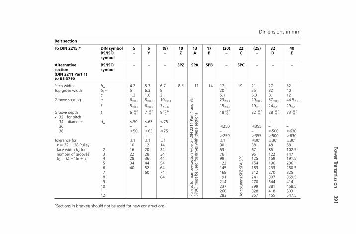
Power Transm
ission391
Belt section
To DIN 2215:* DIN symbol 5 6 (8) 10 13 17 (20) 22 (25) 32 40BS/ISO – Y – Z A B – C – D Esymbol
Alternative BS/ISO – – – SPZ SPA SPB – SPC – – –section symbol (DIN 2211 Part 1) to BS 3790
Pitch width bw 4.2 5.3 6.7 8.5 11 14 17 19 21 27 32Top grove width b1� 5 6.3 8 20 25 32 40
c 1.3 1.6 2 5.1 6.3 8.1 12Groove spacing e 6�0.3 8�0.3 10�0.3 23�0.4 29�0.5 37�0.6 44.5�0.3
f 5�0.5 6�0.5 7�0.6 15�0.8 19�1 24�2 29�2
Groove depth t 6�00.6 7�
00.6 9�
00.6 18�
00.6 22�
00.6 28�
00.6 33�
00.6
x 32 for pitch 34 diameter dw �50 �63 �75 – – – –36 – – – �250 �355 – –38 �50 �63 75 – – �500 �630
– – – �250 �355 �500 �630Tolerance for �1 �1 �1 �1 �30’ �30’ �30’
x � 32 � 38 Pulley 1 10 12 14 30 38 48 58face width b2 for 2 16 20 24 53 67 85 102.5number of grooves: 3 22 28 34 76 96 122 147b2 � (Z �1)e � 2 4 28 36 44 99 125 159 191.5
5 34 44 54 122 154 196 2366 40 52 64 145 183 233 280.57 60 74 168 212 270 3258 84 191 241 307 369.59 214 270 344 414
10 237 299 381 458.511 260 328 418 50312 283 357 455 547.5
*Sections in brackets should not be used for new constructions.
As
colu
mns
SPZ
SPA
SPB
Pulle
ys f
or n
arro
w-s
ectio
n V-
belts
(DIN
221
1 Pa
rt 1
and
BS
3790
) mus
t be
use
d fo
r dr
ives
with
the
se s
ectio
ns
Dimensions in mm

5.2.11 Deep-groove pulleys
392M
echanical Engineer’s Pocket Book
Rz100f
t
f
a
bw
eb1
b2
f
Rz1
00
Rz1
00
Rz2
5
Breakcorners
Single-groove Multi-groove
cd
w

Power Transm
ission393
Belt section
To DIN 7753 Part 1 DIN symbol SPZ SPA SPB SPC 19and BS 3790 BS/ISO symbol SPZ SPA SPB SPC –
To DIN 2215 DIN symbol 10 13 17 22 –and BS 3790 BS/ISO symbol Z A B C –
Pitch width bw 8.5 11 14 19 16
Increased groove width b1� � � 34° 11 15 18.9 26.3 22.1� � 38° 11.3 15.4 19.5 27.3 22.9c 4 6.5 8 12 10
Groove spacing e 14�0.3 18�0.3 23�0.4 31�0.5 27�0.5f 9�0.6 11.5�0.6 14.5�0.8 20�1 17�1
Increased groove depth tmin 13 18 22.5 31.5 26� 34� for pitch diameter dw 63–80 90–118 140–190 224–315 180–250
38� with belts to DIN 7753 1 and BS 3790 �80 �118 �190 �315 �250
� 34� for pitch diameter dw 50–80 71–118 112–190 180–315 –38� with belts to DIN 2215
and BS 3790 �80 �118 �190 �315 �250
Tolerance for � 34°�38° �1° �1° �1° �0.5° �1°Pulley face width b2 for number of 1 18 23 29 40 34grooves z: b2 � (z � 1)e � 2f 2 32 41 52 71 61
3 46 59 75 102 884 60 77 98 133 1155 74 95 121 164 1426 88 113 144 195 1697 102 131 167 226 1968 116 149 190 257 2239 130 167 213 288 25010 144 185 236 319 27711 158 203 259 350 30412 172 221 282 381 331
Minimum pulley diameter must be adhered to. Not to be used for banded V-belts.
Dimensions in mm
5.2.12 Synchronous belt drives: introduction
Synchronous (toothed) belt drives are now widely used in place of traditional, roller chaindrives for many applications. Unlike a flat belt or a V-belt the toothed belt cannot slip,therefore it can be used where the rotation of input (driver) and output (driven) elementsof a system must always be synchronized.
The main advantages of synchronous-belt drives compared with traditional roller chaindrives are as follows:
1. Substantially lower cost.2. Quieter running.3. Ability to operate in environments which would be hostile to a roller chain drive.4. No need for lubrication of the drive.5. The elastomer material from which the belt is made tends to absorb vibrations rather
than transmit them.
Synchronous-belt drive applications are found where their special properties can beexploited. For example:
1. Office equipment where quiet running and lack of lubrication is important.2. Food processing machinery where conventional lubrication, necessary with a chain
drive, might contaminate the foodstuffs being processed.3. Motor vehicle camshaft drives where synchronous, trouble-free, quiet, lubrication-
free, smooth running is required.4. The coupling of stepper motors and servo-motors to the feed mechanisms of computer
controlled machine tools where synchronous, trouble-free, vibration-free, smoothrunning is required.
The following tables of synchronous-belt data and associated toothed pulley data havebeen selected to assist in the design of synchronous-belt drive systems.
Construction
Synchronous-drive belts are composed of:● polychloroprene teeth and backing,● polyamide fabric facing,● glass fibre cords.
Polychloroprene teeth and backingThe teeth and belt backing are made from highly loadable polychloroprene-based elasto-mer materials, firmly bonded to the tension member and fabric facing.
Polychloroprene backing
Polyamide fabric facing
Polychloroprene teeth
Glass fibre cords
394 Mechanical Engineer’s Pocket Book
H6508-Ch05.2.qxd 9/12/05 4:49 PM Page 394
Polyamide fabric facingLasting protection of the teeth is an essential precondition for smooth drive operation anda long belt life. This is guaranteed by using tough, wear-resistant polyamide fabric with alow coefficient of friction.
Glass fibre cordsSynchronous drives call for maximum length stability and tensile strength of the belt. Theserequirements are optimally met by low-stretch glass fibre cords helically wound over theentire belt width. Lateral mistracking is minimized by using S/Z cords arranged in pairs.
PropertiesConstant angular velocity and uniform speed transmissionIn much the same manner as the teeth on a gear, the teeth of the belt make positiveengagement with the mating tooth spaces on the pulleys. The positive-grip drive principleensures synchronous operation and constant circumferential speed.
Freedom from high tensionThe tooth forming principle requires only a very low belt tensioning and so the load onaxles and bearings is kept to a minimum.
High-power transmissionHigh-power transmission is guaranteed by the combination of the extra-stiff teeth and thewear-resistant fabric facing as well as by the tension member’s high resistance to dynamic load.
High-speed ratioReliable drive function is achieved through positive engagement, even with small arcs ofcontact and small pulley diameters.
Minimal space requirementsHigh dynamic loadability and high-power transmission capacity allow the use of smallpulley diameters and short centre distances. This enables designers to design economicaldrives which are not only compact but also light in weight.
High belt speedLow inertia forces and outstanding flex life ensure reliable drive systems up to belt speedsof 60 m/s.
Quiet operationThe supple belt design with fabric-faced rubber teeth in combination with metal or plas-tic pulleys reduces drive noise to a minimum.
Freedom from lubrication and maintenanceSYNCHROBELT® synchronous drive belts are maintenance free. They need no lubricationor retensioning. Constant belt tension is guaranteed by the use of high-strength glassfibre cords as the load-bearing element.
High efficiencyThe flexible and supple belt design as well as optimum dimensional match between the belttoothing and pulley tooth spacing allow virtually friction-free drives with an efficiency of 98%.
CONTI SYNCHROBELT® synchronous drive beltsCONTI SYNCHROBELT® synchronous drive belts have the following standard properties.They are resistant to:
● certain oils● ozone● temperatures ranging from �40°C to 100°C and are● unaffected by tropical climates● insensitive to weathering.
Power Transmission 395
H6508-Ch05.2.qxd 9/12/05 4:49 PM Page 395

DesignationSYNCHROBELT® synchronous drive belts are fully specified by a coding system based onDIN ISO 5296 and showing the following:
● Pitch length in tenths of an inch.● The pitch length of a synchronous drive belt is equal to its overall circumference, meas-
ured along the pitch line which keeps the same length when the belt is bent. The pitchline lies in the centre of the tension member and can only be precisely located with theaid of suitable measuring fixtures. More details are given Section 5.2.17 under ‘Lengthmeasurement’.
● Tooth pitch.● The tooth pitch is the linear distance between two adjacent teeth along the pitch line.● Belt width in hundredths of an inch.● Belt width and belt width reference are identical.
ExampleSYNCHROBELT® synchronous drive belt 1100 H 1001100→pitch length 110 in. � 2794.0 mmH→tooth pitch 0.5 in. � 12.7 mm100→belt width 1 in. � 25.4 mm
The number of teeth z is the function of pitch length Lw and pitch t:
Available sizes
PitchesSYNCHROBELT® synchronous drive belts are supplied in six tooth pitch sizes. They complywith DIN ISO 5296 standard and can be used internationally. Stock pitches and theirdimensions are shown in the above table.
LengthsSYNCHROBELT® synchronous drive belts are available in lengths to cover a broad range ofapplications. In addition, special belt lengths can be furnished on a made-to-order basis.For stock lengths, refer to tables in MXL pitch, XL pitch, L pitch, H pitch, XH pitch and XXHpitch on pages 396–402.
WidthsStock widths are contained in the tables for stock lengths. Non-stock widths are alsoavailable on request.
t
s
y
h t
rr
ra h su
zLwt
�
396 Mechanical Engineer’s Pocket Book
Cross-section of synchronous drive belt.
H6508-Ch05.2.qxd 9/12/05 4:49 PM Page 396

Power Transm
ission397
Parameters
Pitch DIN ISO code MXL XL L H XH XXH
Tooth pitch t mm 2.032 5.080 9.525 12.700 22.225 31.750in. 0.080 0.200 0.375 0.500 0.875 1.250
Flank angle � degrees 40 50 40 40 40 40Belt thickness hs mm 1.14 2.3 3.6 4.3 11.2 15.7Tooth height ht mm 0.51 1.27 1.91 2.29 6.35 9.53Top width of tooth s mm 1.14 2.57 4.65 6.12 12.57 19.05Top radius ra mm 0.13 0.38 0.51 1.02 1.19 1.52Bottom radius rr mm 0.13 0.38 0.51 1.02 1.57 2.29Pitch zone u mm 0.254 0.254 0.381 0.686 1.397 1.524Weight (belt width 25.4 mm) kg/m 0.013 0.016 0.089 0.117 0.235 0.321Range of pitch lengths Lw:
From mm 109.73 152.40 314.33 609.60 1289.05 1778.00To mm 920.50 1473.20 1524.00 4318.00 4445.00 4572.00
Stock widths b:From mm 3.18 6.35 12.7 19.05 50.8 50.8To mm 6.35 25.4 76.2 127.0 177.8 127.0
5.2.13 Synchronous belt drives: belt types and sizes
MXL pitchTooth pitch 2.032 mm (0.080 in.)
Stock lengths
Length code Pitch No. of Length code Pitch No. of length teeth z length teeth z
Lw (mm) Lw (mm)
43.2 MXL 109.73 54 91.2 MXL 231.65 11444.0 MXL 111.76 55 96.0 MXL* 243.84 12044.8 MXL* 113.79 56 97.6 MXL 247.90 12246.4 MXL* 117.86 58 98.4 MXL* 249.94 12348.0 MXL 121.92 60 100.8 MXL 256.06 12654.5 MXL 138.18 68 112.0 MXL* 284.48 14056.0 MXL* 142.24 70 120.0 MXL* 304.80 15056.8 MXL 144.27 71 132.0 MXL* 335.28 16557.6 MXL* 146.30 72 136.0 MXL 345.44 17060.0 MXL* 152.40 75 140.0 MXL 355.60 17564.0 MXL* 162.56 80 144.0 MXL 365.76 18065.6 MXL* 166.62 82 147.2 MXL 373.89 18467.2 MXL 170.69 84 180.0 MXL* 457.20 22568.0 MXL* 172.72 85 188.8 MXL* 479.55 23670.4 MXL* 178.81 88 200.8 MXL* 510.03 25172.0 MXL 182.88 90 204.8 MXL* 520.19 25675.2 MXL 191.01 94 238.4 MXL* 605.54 29877.6 MXL* 197.10 97 277.6 MXL 705.10 34780.0 MXL* 203.20 100 282.4 MXL* 717.30 35380.8 MXL* 205.23 101 292.0 MXL* 741.68 36582.4 MXL* 209.30 103 320.0 MXL* 812.80 40084.0 MXL 213.36 105 347.2 MXL* 881.89 43484.8 MXL* 215.39 106 362.4 MXL* 920.50 45388.0 MXL 223.52 110 370.4 MXL* 940.82 46389.6 MXL* 227.58 112 398.4 MXL* 1011.94 49890.4 MXL 229.62 113 404.0 MXL* 1026.16 505
* Made-to-order belts.
Stock widths
Width reference 012 019 025Width (mm) 3.18 4.76 6.35
1.14
1.14
0.51
2.032
398 Mechanical Engineer’s Pocket Book
Belts with special characteristicsSYNCHROBELT® synchronous drive belts have the standard properties listed on Page 6.Consult our engineers for special types.
H6508-Ch05.2.qxd 9/12/05 4:49 PM Page 398
Power Transmission 399
XL pitchTooth pitch 5.080 mm (0.200 in.)
Stock lengths
Length code Pitch No. of Length Pitch No. of length teeth z code length teeth z
Lw (mm) Lw (mm)
60 XL 152.40 30 136 XL* 345.44 6870 XL 177.80 35 138 XL* 350.62 6980 XL 203.20 40 140 XL 355.60 7086 XL* 218.44 43 148 XL* 376.92 7490 XL 228.60 45 150 XL 381.00 7592 XL* 233.68 46 156 XL* 396.24 7894 XL* 238.76 47 160 XL 406.40 8096 XL* 243.84 48 162 XL* 411.48 81100 XL 254.00 50 168 XL* 426.72 84102 XL* 259.08 51 170 XL 431.80 85106 XL* 269.24 53 174 XL* 441.96 87108 XL* 274.32 54 176 XL* 447.04 88110 XL 279.40 55 178 XL* 452.12 89112 XL* 284.48 56 180 XL 457.20 90116 XL* 294.84 58 182 XL* 462.28 91118 XL* 299.72 59 184 XL* 467.36 92120 XL 304.80 60 188 XL* 477.52 94124 XL* 314.96 62 190 XL 482.60 95126 XL* 320.04 63 196 XL* 497.82 98130 XL 330.20 65 200 XL 508.00 100134 XL* 340.36 67
* Made-to-order belts.
Stock widths
Width reference 025 031 037 050 075 100Width (mm) 6.35 7.94 9.53 12.7 19.05 25.4
2.3
1.27
2.57
5.080
H6508-Ch05.2.qxd 9/12/05 4:49 PM Page 399

XL pitch (continued)Tooth pitch 5.080 mm (0.200 in.)
Stock lengths
Length code Pitch No. of Length Pitch No. of length teeth z code length teeth z
Lw (mm) Lw (mm)
210 XL 533.40 106 322 XL* 817.88 161220 XL 558.80 110 330 XL* 838.20 165230 XL 584.20 115 340 XL* 863.60 170240 XL 609.60 120 344 XL* 873.76 172244 XL* 619.76 122 350 XL* 889.00 175248 XL* 629.92 124 380 XL* 965.20 190250 XL 635.00 125 382 XL* 970.28 191260 XL 660.40 130 388 XL* 985.52 194270 XL* 685.80 135 392 XL* 995.68 196272 XL* 690.88 136 412 XL* 1046.48 206274 XL* 695.96 137 414 XL* 1051.56 207280 XL* 711.20 140 438 XL* 1112.52 219286 XL* 726.44 143 460 XL* 1168.40 230290 XL* 736.60 145 498 XL* 1264.92 249296 XL* 751.84 148 506 XL* 1285.24 253300 XL* 762.00 150 514 XL* 1305.56 257306 XL* 777.24 153 580 XL* 1473.20 290316 XL* 802.64 158 630 XL* 1600.20 315
* Made-to-order belts.
Stock widths
Width reference 025 031 037 050 075 100Width (mm) 6.35 7.94 9.53 12.7 19.05 25.4
5.080
2.57
2.3
1.27
400 Mechanical Engineer’s Pocket Book
H6508-Ch05.2.qxd 9/12/05 4:49 PM Page 400
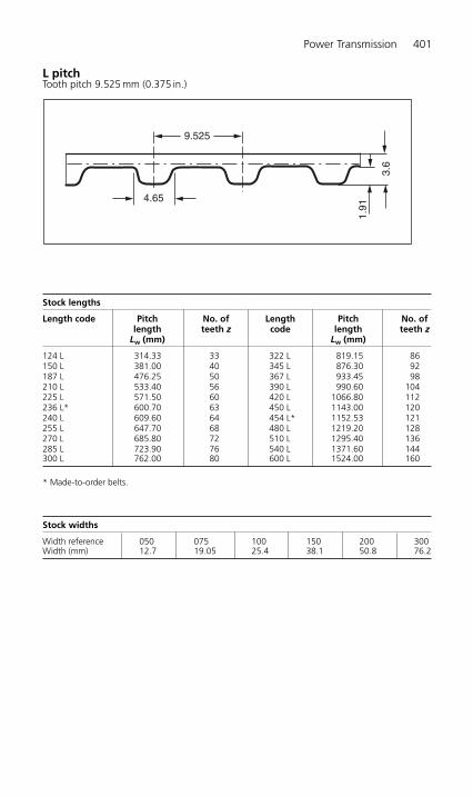
Power Transmission 401
Stock lengths
Length code Pitch No. of Length Pitch No. of length teeth z code length teeth z
Lw (mm) Lw (mm)
124 L 314.33 33 322 L 819.15 86150 L 381.00 40 345 L 876.30 92187 L 476.25 50 367 L 933.45 98210 L 533.40 56 390 L 990.60 104225 L 571.50 60 420 L 1066.80 112236 L* 600.70 63 450 L 1143.00 120240 L 609.60 64 454 L* 1152.53 121255 L 647.70 68 480 L 1219.20 128270 L 685.80 72 510 L 1295.40 136285 L 723.90 76 540 L 1371.60 144300 L 762.00 80 600 L 1524.00 160
* Made-to-order belts.
Stock widths
Width reference 050 075 100 150 200 300Width (mm) 12.7 19.05 25.4 38.1 50.8 76.2
L pitchTooth pitch 9.525 mm (0.375 in.)
3.6
1.91
4.65
9.525
H6508-Ch05.2.qxd 9/12/05 4:49 PM Page 401
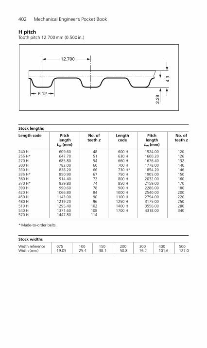
402 Mechanical Engineer’s Pocket Book
H pitchTooth pitch 12.700 mm (0.500 in.)
Stock lengths
Length code Pitch No. of Length Pitch No. of length teeth z code length teeth z
Lw (mm) Lw (mm)
240 H 609.60 48 600 H 1524.00 120255 H* 647.70 51 630 H 1600.20 126270 H 685.80 54 660 H 1676.40 132300 H 782.00 60 700 H 1778.00 140330 H 838.20 66 730 H* 1854.20 146335 H* 850.90 67 750 H 1905.00 150360 H 914.40 72 800 H 2032.00 160370 H* 939.80 74 850 H 2159.00 170390 H 990.60 78 900 H 2286.00 180420 H 1066.80 84 1000 H 2540.00 200450 H 1143.00 90 1100 H 2794.00 220480 H 1219.20 96 1250 H 3175.00 250510 H 1295.40 102 1400 H 3556.00 280540 H 1371.60 108 1700 H 4318.00 340570 H 1447.80 114
* Made-to-order belts.
Stock widths
Width reference 075 100 150 200 300 400 500Width (mm) 19.05 25.4 38.1 50.8 76.2 101.6 127.0
2.29
4.3
6.12
12.700
H6508-Ch05.2.qxd 9/12/05 4:49 PM Page 402
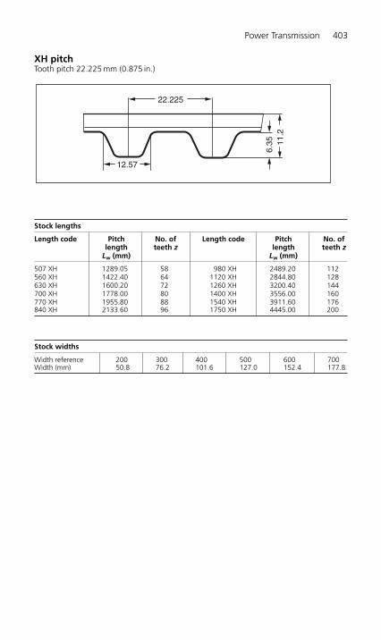
Power Transmission 403
XH pitchTooth pitch 22.225 mm (0.875 in.)
Stock lengths
Length code Pitch No. of Length code Pitch No. of length teeth z length teeth z
Lw (mm) Lw (mm)
507 XH 1289.05 58 980 XH 2489.20 112560 XH 1422.40 64 1120 XH 2844.80 128630 XH 1600.20 72 1260 XH 3200.40 144700 XH 1778.00 80 1400 XH 3556.00 160770 XH 1955.80 88 1540 XH 3911.60 176840 XH 2133.60 96 1750 XH 4445.00 200
Stock widths
Width reference 200 300 400 500 600 700Width (mm) 50.8 76.2 101.6 127.0 152.4 177.8
11.2
6.35
22.225
12.57
H6508-Ch05.2.qxd 9/12/05 4:49 PM Page 403

5.2.14 Synchronous belt drives: pulleys
The right quality and the right choice of pulleys are all-important factors affecting the per-formance of a synchronous-belt drive. They are precision made and machined by specialmilling cutters accurately to pitch so as to ensure precise meshing of the teeth.
Pulleys for synchronous-belt drives should be manufactured to DIN ISO 5294 specifica-tions and can be obtained from your nearest pulley stockist.
Some useful pulley data is given below.
DesignationSYNCHROBELT® pulleys bear the following designation:
● Number of teeth● The number of teeth is calculated from the pitch circumference and the pitch as follows:
Tooth pitchTooth pitch is the distance between two reference points on adjacent teeth at the perimeterof the pitch diameter. The pitch diameter is larger than the outside diameter of the pulley bydouble the pitch zone of the corresponding belt and is located at the pitch line of the belt.
zU
t
d
t� �
�w w
404 Mechanical Engineer’s Pocket Book
XXH pitchTooth pitch 31.750 mm (1.250 in.)
Stock lengths
Length code Pitch length No. of Length code Pitch length No. of Lw (mm) teeth z Lw (mm) teeth z
700 XXH 1778.00 56 1200 XXH 3048.00 96800 XXH 2032.00 64 1400 XXH 3556.00 112900 XXH 2286.00 72 1600 XXH 4064.00 1281000 XXH 2540.00 80 1800 XXH 4572.00 144
Stock widths
Width reference 200 300 400 500Width (mm) 50.8 76.2 101.6 127.0
19.05
15.7
9.53
31.750
H6508-Ch05.2.qxd 9/12/05 4:49 PM Page 404

Power Transmission 405
Pulley width in hundredths of an inchThe width reference indicates the width of the matching belt. Precise pulley widths andtheir corresponding belt widths are contained in the Table in p. 407.
ExampleSYNCHROBELT® pulley 28 H 10028→28 teethH→tooth pitch 0.500 in. � 12.700 mm100→width reference for a 1 in. � 25.4 mm wide synchronous drive belt
MaterialsThe choice of material depends on the size of the pulley and the power to be transmit-ted. The most widely used materials are:
● aluminium alloy: AlCuMgPb F 36 or F 38● steel: St 9 S20K● grey cast iron: GG-25● plastic: PA 6 and 6.6, POM, PBTP, PC
Tooth space measurementsSynchronous-belt drives may be fitted with pulleys with straight tooth flanks or with invo-lute toothing. The type of pulley is determined by the manufacturing process and theintended application.
Table in p. 404 shows the tooth space measurements for pulleys with straight toothflanks. These are not now generally used.
With an involute tooth profile, tooth space measurements may vary depending on thepulley diameter and so an elaborate table would be required to specify involute toothingdimensions. Table in p. 406 therefore shows the hob cutter measurements for pulleys withinvolute toothing.
Pulleys with straight tooth flanks
Tooth space with straight flanks.
r t
r b
bw
h g
t
u
g
d w d a
H6508-Ch05.2.qxd 9/12/05 4:49 PM Page 405

406M
echanical Engineer’s Pocket Book
Pitch MXL XL L H XH XXH
Tooth pitch t 2.032 5.080 9.525 12.700 22.225 31.750
Root width of tooth space bw 0.84�0.05 1.32�0.05 3.05�0.10 4.19�0.13 7.90�0.15 12.17�0.18
Depth of tooth space hg 0.69�00.05 1.65�0
0.08 2.67�0
0.10 3.05�0
0.13 7.14�
00.13 10.31�0
0.13
Angle of tooth space � degrees 40�3 50�3 40�3 40�3 40�3 40�3
Bottom radius rb max 0.25 0.41 1.19 1.60 1.98 3.96
Top radius rt 0.13�00.05 0.64�0
0.05 1.17�0
0.13 1.60�0
0.13 2.39�0
0.13 3.18�0
0.13
2 � pitch zone u 0.508 0.508 0.762 1.372 2.794 3.048
Dimensions in mm
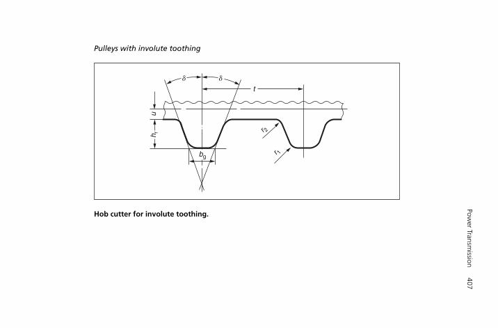
Power Transm
ission407
r 2
r 1bg
t
h ru
dd
Pulleys with involute toothing
Hob cutter for involute toothing.

408M
echanical Engineer’s Pocket Book
Pitch MXL XL L H XH XXH
Tooth pitch t 2.032 5.080 9.525 12.700 22.225 31.750
No. of pulley teeth 1 10–23 10 10 14–19 18 18
2 24 �19
Flank angle 2 � � degrees 1 56 50 40 40 40 40
2 40 40
Bottom width of tooth bg 1 0.61�00.05 1.27�0
0.05 3.10�0
0.05 4.24�0
0.05 7.59�0
0.05 11.61�0
0.05
2 0.67�00.05
Height of tooth hr 0.64�00.05 1.40�0
0.05 2.13�0
0.05 2.59�0
0.05 6.88�0
0.05 10.29�0
0.05
Top radius r1 0.30�0.03 0.61�0.03 0.86�0.03 1.47�0.03 2.01�0.03 2.69�0.03
Bottom radius r2 1 0.23�0.03 0.61�0.03 0.53�0.03 1.04�0.03 1.93�0.03 2.82�0.03
2 0.23�0.03 1.42�0.03
2 � pitch zone u mm 0.508 0.508 0.762 1.372 2.794 3.048
Tolerance for all tooth pitches � �0.003
Dimensions in mm

Power Transmission 409
Pulley widthsWidth references, nominal widths and minimum toothing widths for pulleys with andwithout flanges are listed in following Table. When using pulleys with one flange, theminimum toothing width for pulleys with two flanges is recommended.
Pulley widths (all dimensions in mm)
Pitch Width Nominal Minimum toothing widthreference width
with flanges without flanges
MXL 012 3.2 3.8 5.6018 4.8 5.3 7.1025 6.4 7.1 8.9
XL 025 6.4 7.1 8.9031 7.9 8.6 10.4037 9.5 10.4 12.2
H 075 19.1 20.3 24.8100 25.4 26.7 31.2150 38.1 39.4 43.9200 50.8 52.8 57.3300 76.2 79.0 83.5
XH 200 50.8 56.6 62.6300 76.2 83.8 89.8400 101.6 110.7 116.7
XXH 200 50.8 56.6 64.1300 76.2 83.8 91.3400 101.6 110.7 118.2500 127.0 137.7 145.2
Pulley diametersPitch and outside diameters for SYNCHROBELT® pulleys, together with the number ofteeth are as follows:
Synchrobelt pulleys (MXL pitch) Synchrobelt pulleys (H pitch)Range: 10 teeth: P/D 6.47 mm, Range: 16 teeth: P/D 64.68 mm,O/D 5.96 mm to 150 teeth: P/D O/D 63.61 mm to 150 teeth: P/D97.02 mm, 606.38 mm,O/D 96.51 mm in steps of 1 tooth O/D 605.01 mm in steps of 1 tooth
Synchrobelt pulleys (XL pitch) Synchrobelt pulleys (XH pitch)Range: 10 teeth: P/D 16.17 mm, Range: 20 teeth: P/D 141.49 mm, O/DO/D 15.66 mm to 150 teeth: P/D 138.69 mm to 150 teeth: P/D 242.55 mm, 1061.17 mm,O/D 242.04 mm in steps of 1 tooth O/D 1058.37 mm in steps of 1 tooth
Synchrobelt pulleys (L pitch) Synchrobelt pulleys (XXH pitch)Range: 12 teeth: P/D 36.38 mm, Range: 22 teeth: P/D 222.34 mm, O/DO/D 35.62 mm to 150 teeth: P/D 219.29 mm to 120 teeth: P/D 454.78 mm, 1212.79 mm,O/D 454.02 mm in steps of 1 tooth O/D 1209.71 mm in steps of 1 tooth
(P/D � pitch diameter, O/D � overall diameter)
H6508-Ch05.2.qxd 9/12/05 4:49 PM Page 409
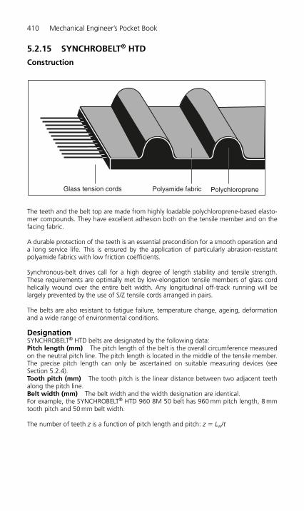
5.2.15 SYNCHROBELT® HTD
Construction
The teeth and the belt top are made from highly loadable polychloroprene-based elasto-mer compounds. They have excellent adhesion both on the tensile member and on thefacing fabric.
A durable protection of the teeth is an essential precondition for a smooth operation anda long service life. This is ensured by the application of particularly abrasion-resistantpolyamide fabrics with low friction coefficients.
Synchronous-belt drives call for a high degree of length stability and tensile strength.These requirements are optimally met by low-elongation tensile members of glass cordhelically wound over the entire belt width. Any longitudinal off-track running will belargely prevented by the use of S/Z tensile cords arranged in pairs.
The belts are also resistant to fatigue failure, temperature change, ageing, deformationand a wide range of environmental conditions.
DesignationSYNCHROBELT® HTD belts are designated by the following data:Pitch length (mm) The pitch length of the belt is the overall circumference measuredon the neutral pitch line. The pitch length is located in the middle of the tensile member.The precise pitch length can only be ascertained on suitable measuring devices (seeSection 5.2.4).Tooth pitch (mm) The tooth pitch is the linear distance between two adjacent teethalong the pitch line.Belt width (mm) The belt width and the width designation are identical.For example, the SYNCHROBELT® HTD 960 8M 50 belt has 960 mm pitch length, 8 mmtooth pitch and 50 mm belt width.
The number of teeth z is a function of pitch length and pitch: z � Lw/t
Glass tension cords Polyamide fabric Polychloroprene
410 Mechanical Engineer’s Pocket Book
H6508-Ch05.2.qxd 9/12/05 4:49 PM Page 410
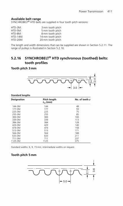
Power Transmission 411
Available belt rangeSYNCHROBELT® HTD belts are supplied in four tooth pitch versions:
HTD-3M: 3 mm tooth pitchHTD-5M: 5 mm tooth pitchHTD-8M: 8 mm tooth pitchHTD-14M: 14 mm tooth pitchHTD-20M: 20 mm tooth pitch
The length and width dimensions that can be supplied are shown in Section 5.2.11. Therange of pulleys is illustrated in Section 5.2.16.
5.2.16 SYNCHROBELT® HTD synchronous (toothed) belts:tooth profiles
Tooth pitch 3 mm
Standard lengths
Designation Pitch length No. of teeth zLw (mm)
144-3M 144 48177-3M 177 59225-3M 225 75255-3M 255 85300-3M 300 100339-3M 339 113384-3M 384 128420-3M 420 140474-3M 474 158513-3M 513 171564-3M 564 188633-3M 633 211711-3M 711 237
1125-3M 1125 375
Standard widths: 6, 9, 15 mm; intermediate widths on request.
Tooth pitch 5 mm
3.6
2.1
5.0
2.4
1.2
3.0
H6508-Ch05.2.qxd 9/12/05 4:49 PM Page 411
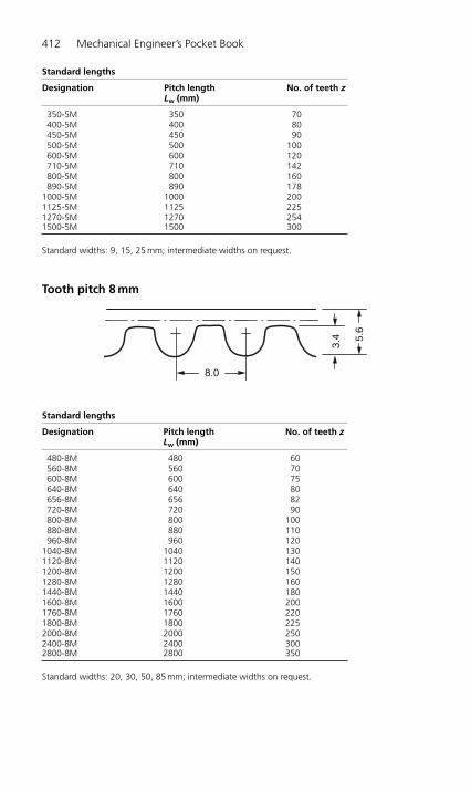
Standard lengths
Designation Pitch length No. of teeth zLw (mm)
350-5M 350 70400-5M 400 80450-5M 450 90500-5M 500 100600-5M 600 120710-5M 710 142800-5M 800 160890-5M 890 178
1000-5M 1000 2001125-5M 1125 2251270-5M 1270 2541500-5M 1500 300
Standard widths: 9, 15, 25 mm; intermediate widths on request.
Tooth pitch 8 mm
Standard lengths
Designation Pitch length No. of teeth zLw (mm)
480-8M 480 60560-8M 560 70600-8M 600 75640-8M 640 80656-8M 656 82720-8M 720 90800-8M 800 100880-8M 880 110960-8M 960 120
1040-8M 1040 1301120-8M 1120 1401200-8M 1200 1501280-8M 1280 1601440-8M 1440 1801600-8M 1600 2001760-8M 1760 2201800-8M 1800 2252000-8M 2000 2502400-8M 2400 3002800-8M 2800 350
Standard widths: 20, 30, 50, 85 mm; intermediate widths on request.
5.6
3.4
8.0
412 Mechanical Engineer’s Pocket Book
H6508-Ch05.2.qxd 9/12/05 4:49 PM Page 412
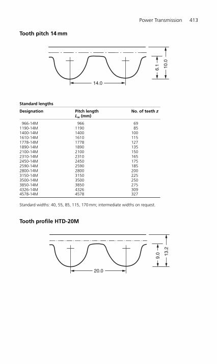
Power Transmission 413
Tooth pitch 14 mm
Standard lengths
Designation Pitch length No. of teeth zLw (mm)
966-14M 966 691190-14M 1190 851400-14M 1400 1001610-14M 1610 1151778-14M 1778 1271890-14M 1890 1352100-14M 2100 1502310-14M 2310 1652450-14M 2450 1752590-14M 2590 1852800-14M 2800 2003150-14M 3150 2253500-14M 3500 2503850-14M 3850 2754326-14M 4326 3094578-14M 4578 327
Standard widths: 40, 55, 85, 115, 170 mm; intermediate widths on request.
Tooth profile HTD-20M
13.2
9.0
20.0
10.0
6.1
14.0
H6508-Ch05.2.qxd 9/12/05 4:49 PM Page 413
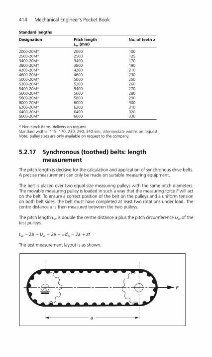
Standard lengths
Designation Pitch length No. of teeth zLw (mm)
2000-20M* 2000 1002500-20M* 2500 1253400-20M* 3400 1703800-20M* 3800 1904200-20M* 4200 2104600-20M* 4600 2305000-20M* 5000 2505200-20M* 5200 2605400-20M* 5400 2705600-20M* 5600 2805800-20M* 5800 2906000-20M* 6000 3006200-20M* 6200 3106400-20M* 6400 3206600-20M* 6600 330
* Non-stock items, delivery on request.Standard widths: 115, 170, 230, 290, 340 mm; intermediate widths on request.Note: pulley sizes are only available on request to the company.
5.2.17 Synchronous (toothed) belts: length measurement
The pitch length is decisive for the calculation and application of synchronous drive belts.A precise measurement can only be made on suitable measuring equipment.
The belt is placed over two equal size measuring pulleys with the same pitch diameters.The movable measuring pulley is loaded in such a way that the measuring force F will acton the belt. To ensure a correct position of the belt on the pulleys and a uniform tensionon both belt sides, the belt must have completed at least two rotations under load. Thecentre distance a is then measured between the two pulleys.
The pitch length Lw is double the centre distance a plus the pitch circumference Uw of thetest pulleys:
Lw � 2a � Uw � 2a � �dw � 2a � zt
The test measurement layout is as shown.
F
a
414 Mechanical Engineer’s Pocket Book
H6508-Ch05.2.qxd 9/12/05 4:49 PM Page 414

Power Transmission 415
5.2.18 SYNCHROBELT® HTD toothed pulleys: preferredsizes
Tooth pitch 3 mm
Dimensions in mm
No. of Pitch Outside Flanged Stock Finished bore teeth diameter diameter pulley bore diameter z dw da diameter db diameter dv dF max
10 9.55 8.79 12 3 312 11.46 10.70 14 3 414 13.37 12.61 16 3 615 14.32 13.56 16 3 616 15.28 14.52 18 3 817 16.23 15.47 20 4 818 17.19 16.43 20 4 819 18.14 17.38 21 4 820 19.10 18.34 23 4 1022 21.01 20.25 25 4 1024 22.94 22.16 26 4 1226 24.83 24.07 28 4 1428 26.74 25.98 30 4 1530 28.65 27.89 33 6 1732 30.56 29.80 34 6 1934 32.47 31.71 36 6 2036 34.38 33.62 38 6 2038 36.29 35.53 42 6 2540 38.20 37.44 42 6 2544 42.02 41.26 47 8 2850 47.75 46.99 51 8 3256 53.48 52.72 59 8 3662 59.21 58.45 64 8 4272 68.75 67.99 73 8 50
The relationship between standard belt width and pulley width.
Dimensions in mm
Standard belt Pulley width � Toothed width for width b toothing width w/o flanged pulleys
flanged pulleys
6 11 �99 14 �12
15 20 �18
H6508-Ch05.2.qxd 9/12/05 4:49 PM Page 415
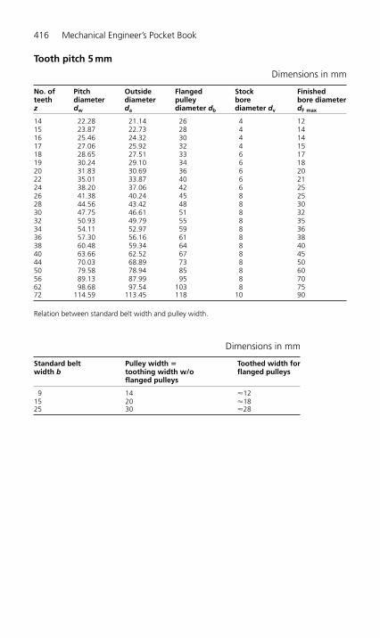
Tooth pitch 5 mm
Dimensions in mm
No. of Pitch Outside Flanged Stock Finished teeth diameter diameter pulley bore bore diameter z dw da diameter db diameter dv dF max
14 22.28 21.14 26 4 1215 23.87 22.73 28 4 1416 25.46 24.32 30 4 1417 27.06 25.92 32 4 1518 28.65 27.51 33 6 1719 30.24 29.10 34 6 1820 31.83 30.69 36 6 2022 35.01 33.87 40 6 2124 38.20 37.06 42 6 2526 41.38 40.24 45 8 2528 44.56 43.42 48 8 3030 47.75 46.61 51 8 3232 50.93 49.79 55 8 3534 54.11 52.97 59 8 3636 57.30 56.16 61 8 3838 60.48 59.34 64 8 4040 63.66 62.52 67 8 4544 70.03 68.89 73 8 5050 79.58 78.94 85 8 6056 89.13 87.99 95 8 7062 98.68 97.54 103 8 7572 114.59 113.45 118 10 90
Relation between standard belt width and pulley width.
Dimensions in mm
Standard belt Pulley width � Toothed width for width b toothing width w/o flanged pulleys
flanged pulleys
9 14 �1215 20 �1825 30 �28
416 Mechanical Engineer’s Pocket Book
H6508-Ch05.2.qxd 9/12/05 4:49 PM Page 416
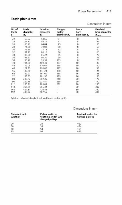
Power Transmission 417
Tooth pitch 8 mm
Dimensions in mm
No. of Pitch Outside Flanged Stock Finished teeth diameter diameter pulley bore bore diameter z dw da diameter db diameter dv dF max
22 56.02 54.65 61 8 3824 61.12 59.75 67 8 4526 66.21 64.84 75 8 5028 71.30 70.08 80 8 5530 76.39 75.13 82 8 6032 81.49 80.16 86 8 6034 86.58 85.22 95 8 7036 91.67 90.30 99 8 7538 96.77 95.39 103 8 7540 101.86 100.49 107 10 8044 112.05 110.67 118 10 9048 122.23 120.86 127 10 9856 142.60 141.23 150 10 12464 162.97 161.60 168 16 13872 183.35 181.97 189 16 15580 203.72 202.35 210 20 17090 229.18 227.81 235 20 190
112 285.21 283.83 292 20 250144 366.69 365.32 – 30 300168 427.81 426.44 – 30 350192 488.92 487.55 – 30 400
Relation between standard belt width and pulley width.
Dimensions in mm
Standard belt Pulley width � Toothed width for width b toothing width w/o flanged pulleys
flanged pulleys
20 26 �2230 38 �3450 58 �5485 94 �90
H6508-Ch05.2.qxd 9/12/05 4:49 PM Page 417
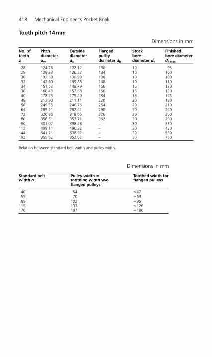
Tooth pitch 14 mm
Dimensions in mm
No. of Pitch Outside Flanged Stock Finished teeth diameter diameter pulley bore bore diameter z dw da diameter db diameter dv dF max
28 124.78 122.12 130 10 9529 129.23 126.57 134 10 10030 133.69 130.99 138 10 10032 142.60 139.88 148 10 11034 151.52 148.79 156 16 12036 160.43 157.68 166 16 13040 178.25 175.49 184 16 14548 213.90 211.11 220 20 18056 249.55 246.76 254 20 21064 285.21 282.41 290 20 24072 320.86 318.06 326 30 26080 356.51 353.71 362 30 29090 401.07 398.28 – 30 330
112 499.11 496.32 – 30 420144 641.71 638.92 – 30 550192 855.62 852.62 – 30 750
Relation between standard belt width and pulley width.
Dimensions in mm
Standard belt Pulley width � Toothed width for width b toothing width w/o flanged pulleys
flanged pulleys
40 54 �4755 70 �6385 102 �95
115 133 �126170 187 �180
418 Mechanical Engineer’s Pocket Book
H6508-Ch05.2.qxd 9/12/05 4:49 PM Page 418
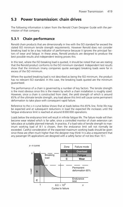
Power Transmission 419
5.3 Power transmission: chain drives
The following information is taken from the Renold Chain Designer Guide with the per-mission of that company.
5.3.1 Chain performance
Renold chain products that are dimensionally in line with the ISO standard far exceed thestated ISO minimum tensile strength requirements. However Renold does not considerbreaking load to be a key indicator of performance because it ignores the principal fac-tors of wear and fatigue. In these areas, Renold products are designed to produce thebest possible results and independent testing proves this.
In this text, where the ISO breaking load is quoted, it should be noted that we are statingthat the Renold product conforms to the ISO minimum standard. Independent test resultsshow that the minimum (many companies quote averages) breaking loads were far inexcess of the ISO minimum.
Where the quoted breaking load is not described as being the ISO minimum, the producthas no relevant ISO standard. In this case, the breaking loads quoted are the minimumguaranteed.
The performance of a chain is governed by a number of key factors. The tensile strengthis the most obvious since this is the means by which a chain installation is roughly sized.However, since a chain is constructed from steel, the yield strength of which is around65% of the ultimate tensile strength, any load above this limit will cause some permanentdeformation to take place with consequent rapid failure.
Reference to the s–n curve below shows that at loads below this 65% line, finite life maybe expected and at subsequent reductions in load the expected life increases until thefatigue endurance limit is reached at around 8 000 000 operations.
Loads below the endurance limit will result in infinite fatigue life. The failure mode will thenbecome wear related which is far safer, since a controlled monitor of chain extension cantake place at suitable planned intervals. In practice, if a load ratio of tensile strength to max-imum working load of 8:1 is chosen, then the endurance limit will not normally beexceeded. Careful consideration of the expected maximum working loads should be givensince these are often much higher than the designer may think! It is also a requirement thatany passenger lift applications are designed with a safety factor of not less than 10:1.
s–n curve
Breakingload
Cycles to failure
Endurancelimit
1 8.0 � 106
Permanentdeformation 65%
Zone Failure mode
Load B
A
C
B
A
Fatigue
Overload
WearC
s
n
H6508-Ch05.3.qxd 9/12/05 4:48 PM Page 419

In most applications the failure mode is designed to be wear and therefore some consid-eration of how a chain behaves in this mode are shown below.
Examination of the wear characteristics graph below shows that chain tends to wear in three distinct phases. The first phase, shown as ‘bedding in’, is a very rapid change inchain length associated with components adjusting to the loads imposed on them. Thedegree of this initial movement will depend to a large extent on the quality of chain used.For example, good component fits, chain preloaded at manufacture, plates assembledsquarely, etc. Renold chain has many features that minimise the degree of bedding in.
The second phase, shown as ‘initial wear’, might also be described as secondary ‘beddingin’. This is caused firstly by the rapid abrasion of local high spots between the mating sur-faces of the pin and bush, and secondly by displacement of material at the bush ends.This is explained more clearly by the inner link assembly diagram shown, where it may beseen that in order to ensure good fatigue life, the bush and plate have a high degree ofinterference fit resulting in a tendency of the bush ends to collapse inwards slightly. Thislocalised bulge will wear rapidly until the pin bears equally along the length of the bush.Renold limits this effect by introducing special manufacturing techniques. Some manu-facturers maintain cylindricity by reducing the interference fit to a very low level. Thisreduces fatigue performance.
d2
d1d1 � d2
Tendency of bush to collapse at assembly
Wear characteristics
Elapsed time (h)
Bedding in Adjust tension
Initial wear
100 200
Projected life 15 000 h
Elo
ng
atio
n (
%)
Steady state wear
420 Mechanical Engineer’s Pocket Book
H6508-Ch05.3.qxd 9/12/05 4:48 PM Page 420

The final steady state of wear will continue at a very low rate until the chain needs renewal. Ina correctly designed and lubricated system, 15 000 h continuous running should be normal.
The reason that wear takes place at all is demonstrated with reference to the Stribeck dia-gram below. It may be seen from this that where two mating surfaces are in contact, thecoefficient of friction is very high at the point of initial movement, known as static fric-tion. The reason for this is that the surface irregularities of the two bodies are interlockedwith little or no separating lubrication layer. As the surface speeds increase, lubricant isdrawn between the two surfaces and friction takes place with some surface contact. Thiscondition is known as ‘mixed friction’. These two conditions result in material loss overtime. With a continuing increase in surface speed, hydrodynamic friction takes place, acondition where there is no metal to metal contact.
If we consider the action of the mating surfaces of the bush and pin during one cycle of atwo sprocket system, it will quickly be realised that these components are stationary withrespect to each other during travel from one sprocket to the other, and accelerate rapidlythrough a very small angle when engaging with the sprocket before coming to rest oncemore. This means that the pin/bush combination is operating between the static and mixedfriction states and that lubrication will therefore be an important aspect of system design.
5.3.2 Wear factors
As already shown, wear takes place from the friction between the mating of the pin andbush. The rate of wear is primarily determined by the bearing area and the specific pres-sure on these surfaces. The hardened layers of the pin and bush are eroded in such a waythat the chain will become elongated.
Elongation may amount to a Maximum of 2% of the nominal length of the chain. Above2% elongation, there can be problems with the chain riding up and jumping the sprocketteeth.
Elongation should be limited to 1% when:
● A sprocket in the system has 90 teeth or more.● Perfect synchronization is required.● Centre distances are greater than recommended and not adjustable.
Stribeck diagram
Rotational speed
Co
effi
cien
t o
f fr
icti
on
Boundary friction
Hydrodynamic frictionMixedfriction
Static friction
Power Transmission 421
H6508-Ch05.3.qxd 9/12/05 4:48 PM Page 421
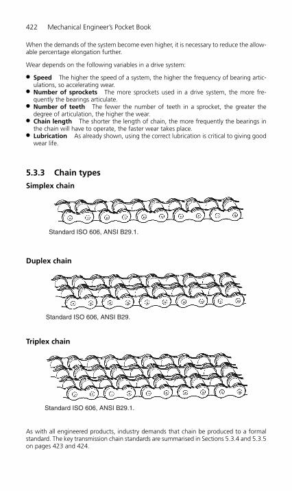
When the demands of the system become even higher, it is necessary to reduce the allow-able percentage elongation further.
Wear depends on the following variables in a drive system:
● Speed The higher the speed of a system, the higher the frequency of bearing artic-ulations, so accelerating wear.
● Number of sprockets The more sprockets used in a drive system, the more fre-quently the bearings articulate.
● Number of teeth The fewer the number of teeth in a sprocket, the greater thedegree of articulation, the higher the wear.
● Chain length The shorter the length of chain, the more frequently the bearings inthe chain will have to operate, the faster wear takes place.
● Lubrication As already shown, using the correct lubrication is critical to giving goodwear life.
5.3.3 Chain types
Simplex chain
Duplex chain
Triplex chain
As with all engineered products, industry demands that chain be produced to a formalstandard. The key transmission chain standards are summarised in Sections 5.3.4 and 5.3.5on pages 423 and 424.
Standard ISO 606, ANSI B29.1.
Standard ISO 606, ANSI B29.
Standard ISO 606, ANSI B29.1.
422 Mechanical Engineer’s Pocket Book
H6508-Ch05.3.qxd 9/12/05 4:48 PM Page 422

5.3.4 International Standards
European StandardChains manufactured to the above standards are covered by ISO 606 and DIN 8187.These standards cover three versions:
● Simplex● Duplex● Triplex
The range of pitch sizes can vary between 4 mm, (0.158 in.) to 114.3 mm, (4.500 in.).
They are characterised by a large pin diameter, especially for the larger pitch sizes. Thisresults in better wear resistance due to the greater bearing area.
The ISO Standard has a simple form of part numbering, for example 1/2 in. pitch duplexchain would be 08B-2.
● The first two digits are the pitch size in 1/16’s of an inch, therefore 08 � 8/16 or 1/2 in.● The letter ‘B’ indicates European Standard.● The suffix two indicates the number of strands in the chain, in this case a duplex chain.
American StandardAmerican Standard chains are covered by ISO 606, ANSI B29.1 and DIN 8188 and eightversions are covered.
● Simplex, duplex and triplex as for the European Standard chains● Quadruplex, 4 strands● Quintuplex, 5 strands● Sextuplex, 6 strands● Octuplex, 8 strands● Decuplex, 10 strands.
The pitch sizes covered by this standard are 1/4 to 3 in. pitch.
American Standard chains have a smaller pin diameter than their European Standardequivalent. Wear resistance is therefore reduced when compared with European Standardchains with the one exception, 5/8 in. pitch. In this case the pin and bush diameter islarger in an American Standard chain.
American Standard chains are normally referred to under the ANSI Standard numberingsystem, for example a 1/2 in. pitch duplex chain would be, ANSI 40-2.
The ANSI numbering system works as follows:
● The first number is the pitch size in 1/8 in.; that is, 4/8 � 1/2 in. pitch.● The second number refers to the chain being a roller chain, 0 � roller chain. A 5 replac-
ing the 0 would indicate a bush chain.● The suffix, as with European Standard chain, refers to the number of strands in the
chain, that is 2 � duplex chain.
ANSI chain is also available in heavy duty options with thicker plates (H) and throughhardened pins (V). An ANSI heavy chain would be specified using these suffixes. That is,
ANSI 140-2HV Duplex, thick plates, through hardened pinANSI 80H Simplex, thick plates
Range of applicationThe transmission chain market worldwide is divided between these two chain standards,based on the economic and historical influences within their regions.
Power Transmission 423
H6508-Ch05.3.qxd 9/12/05 4:48 PM Page 423
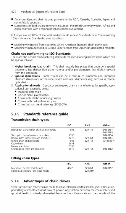
● American Standard chain is used primarily in the USA, Canada, Australia, Japan andsome Asiatic countries.
● European Standard chains dominate in Europe, the British Commonwealth, Africa andAsian countries with a strong British historical involvement.
In Europe around 85% of the total market uses European Standard chain. The remaining15% is American Standard chains found on:
● Machinery imported from countries where American Standard chain dominates.● Machinery manufactured in Europe under licence from American dominated markets.
Chain not conforming to ISO StandardsThere are also Renold manufacturing standards for special or engineered chain which canbe split as follows:
1. Higher breaking load chain This chain usually has plates that undergo a specialtreatment, has thicker side plate material and/or pin diameters that slightly deviatefrom the standards.
2. Special dimensions Some chains can be a mixture of American and EuropeanStandard dimensions or the inner width and roller diameters vary, such as in motor-cycle chains.
3. Applicational needs Special or engineered chain is manufactured for specific appli-cational use, examples being:● Stainless steel chain● Zinc or nickel plated chain● Chain with plastic lubricating bushes● Chains with hollow bearing pins● Chain that can bend sideways (SIDEBOW).
5.3.5 Standards reference guide
Transmission chain types
ISO ANSI Other
Short pitch transmission chain and sprockets 606 B29.1M DIN 8187DIN 8188
Short pitch bush chains and sprockets 1395 DIN 8154Double pitch roller chain and sprockets 1275 B29.3M DIN 8181Oilfield chain and sprockets 606 B29.1M API Spec 7FCycle chains 9633Motorcycle chains 10190Cranked link chain and sprockets 3512 B29.1M DIN 8182
Lifting chain types
ISO ANSI Other
Leaf chain, clevises and sheaves 4347 B29.8M DIN 8152Roller load chains for overhead hoists B29.24M
5.3.6 Advantages of chain drives
Steel transmission roller chain is made to close tolerances with excellent joint articulation,permitting a smooth efficient flow of power. Any friction between the chain rollers andsprocket teeth is virtually eliminated because the rollers rotate on the outside of the
424 Mechanical Engineer’s Pocket Book
H6508-Ch05.3.qxd 9/12/05 4:48 PM Page 424

bushes, independent of bearing pin articulation inside the bush. As a result, very littleenergy is wasted and tests have shown chain to have an efficiency of between 98.4% and98.9%.
This high level of efficiency, achieved by a standard stock chain drive under the correctconditions of lubrication and installation, is equalled only by gears of the highest standardwith teeth ground to very close tolerances.
Roller chain offers a positive, non-slip driving medium. It provides an accurate pitch bypitch positive drive which is essential on synchronised drives such as those to automobileand marine camshafts, packaging and printing machinery. Under conditions of highspeed and peak load when efficiency is also required, the roller chain has proved consist-ently quiet and reliable.
Centre distances between shafts can range from 50 mm up to more than 9 m in a verycompact installation envelope. Drives can be engineered so that the sprocket teeth justclear each other or so that a considerable span is traversed by the chain. In this later cat-egory, double pitch chain comes into its own.
Roller chain has a certain degree of inherent elasticity and this, plus the cushioning effectof an oil film in the chain joints, provides good shock absorbing properties. In addition,the load distribution between a chain and sprocket takes place over a number of teeth,which assists in reducing wear. When, after lengthy service, it becomes necessary toreplace a chain, this is simple and does not normally entail sprocket or bearing removal.
Roller chain minimises loads on the drive motor and driven shaft bearings since no pre-load is required to tension the chain in the static condition.
One chain can drive several shafts simultaneously and in almost any configuration of centredistance or layout. Its adaptability is not limited to driving one or more shafts from a com-mon drive point. It can be used for an infinite variety of devices including reciprocation,racks, cam motions, internal or external gearing, counterbalancing, hoisting or weightsuspension. Segmental tooth or ‘necklace’ chain sprocket rims can be fitted to largediameter drums.
Since there are no elastomeric components involved, chain is tolerant of a wide variety ofenvironmental conditions, including extremes of temperature. Chain is used successfullyin such harsh environments as chemical processing, mining, baking, rock drilling andwood processing. Special coatings can easily be applied for further enhancement.
Roller chain can also be fitted with link plate attachments and extended bearing pins,etc., which allow them to be used for mechanical handling equipment and the operationof mechanisms.
Roller chain drives are available for ratios up to 9:1 and to transmit up to 520 kW at550 rev/min. Beyond this, four matched strands of triplex chain can achieve 3200 kW at300 rev/min.
Roller chain does not deteriorate with the passage of time, the only evidence of age beingelongation due to wear which normally is gradual and can be accommodated by centredistance adjustment or by an adjustable jockey sprocket. Provided a chain drive is selectedcorrectly, properly installed and maintained, a life of 15 000 h can be expected withoutchain failure either from fatigue or wear.
Where complete reliability and long life are essential, chains can be selected on theirassured performance for applications such as hoists for control rods in nuclear reactorsand control systems for aircraft.
Power Transmission 425
H6508-Ch05.3.qxd 9/12/05 4:48 PM Page 425
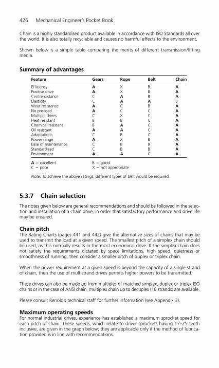
Chain is a highly standardised product available in accordance with ISO Standards all overthe world. It is also totally recyclable and causes no harmful effects to the environment.
Shown below is a simple table comparing the merits of different transmission/liftingmedia.
Summary of advantages
5.3.7 Chain selection
The notes given below are general recommendations and should be followed in the selec-tion and installation of a chain drive, in order that satisfactory performance and drive lifemay be ensured.
Chain pitchThe Rating Charts (pages 441 and 442) give the alternative sizes of chains that may beused to transmit the load at a given speed. The smallest pitch of a simplex chain shouldbe used, as this normally results in the most economical drive. If the simplex chain doesnot satisfy the requirements dictated by space limitations, high speed, quietness orsmoothness of running, then consider a smaller pitch of duplex or triplex chain.
When the power requirement at a given speed is beyond the capacity of a single strandof chain, then the use of multistrand drives permits higher powers to be transmitted.
These drives can also be made up from multiples of matched simplex, duplex or triplex ISOchains or in the case of ANSI chain, multiplex chain up to decuplex (10 strands) are available.
Please consult Renold’s technical staff for further information (see Appendix 3).
Maximum operating speedsFor normal industrial drives, experience has established a maximum sprocket speed foreach pitch of chain. These speeds, which relate to driver sprockets having 17–25 teethinclusive, are given in the graph below; they are applicable only if the method of lubrica-tion provided is in line with recommendations.
Feature Gears Rope Belt Chain
Efficiency A X B APositive drive A X B ACentre distance C A B AElasticity C A A BWear resistance A C B ANo pre-load A C C AMultiple drives C X C AHeat resistant B B C AChemical resistant B A C AOil resistant A A C AAdaptations C B C APower range A X B AEase of maintenance C B B AStandardized C B B AEnvironment A A C A
A � excellent B � goodC � poor X � not appropriate
Note: To achieve the above ratings, different types of belt would be required.
426 Mechanical Engineer’s Pocket Book
H6508-Ch05.3.qxd 9/12/05 4:48 PM Page 426
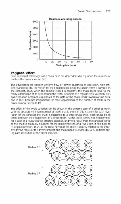
Polygonal effectFour important advantages of a chain drive are dependent directly upon the number ofteeth in the driver sprocket (Z1).
The advantages are smooth uniform flow of power, quietness of operation, high effi-ciency and long life, the reason for their dependence being that chain forms a polygon onthe sprocket. Thus, when the sprocket speed is constant, the chain speed (due to themany sided shape of its path around the teeth) is subject to a regular cyclic variation. Thiscyclic variation becomes less marked as the path of the chain tends towards a true circleand in fact, becomes insignificant for most applications as the number of teeth in thedriver sprocket exceeds 19.
The effect of this cyclic variation can be shown in the extreme case of a driver sprocketwith the absolute minimum number of teeth; that is, three. In this instance, for each revo-lution of the sprocket the chain is subjected to a three-phase cycle; each phase beingassociated with the engagement of a single tooth. As the tooth comes into engagement,for a sixth of a revolution the effective distance, or driving radius from the sprocket centreto the chain is gradually doubled; for the remaining sixth of a revolution, it falls back toits original position. Thus, as the linear speed of the chain is directly related to the effec-tive driving radius of the driver sprocket, the chain speed fluctuates by 50% six times dur-ing each revolution of the driver sprocket.
Radius 1R
Radius 2R
Maximum operating speeds6000
5000
4000
3000
2000
1000
010
Sp
eed
(re
v/m
in)
20 30 40 50 60 70 80Chain pitch (mm)
Power Transmission 427
H6508-Ch05.3.qxd 9/12/05 4:48 PM Page 427

As the graph below shows, the percentage of cyclic speed variation decreases rapidly asmore teeth are added. With the driver sprocket of 19 teeth, therefore, this cyclic speedvariation is negligible; hence we recommend that driver sprockets used in normal appli-cation drives running at medium to maximum speeds, should have not less than 19 teeth.
There are, however, applications where space saving is a vital design requirement and thespeed/power conditions are such that the smaller numbers of teeth (i.e. below 17) giveacceptable performance so that a compact, satisfactory drive is achieved; for example,office machinery, hand operated drives, mechanisms, etc.
The limiting conditions with steady loading for using small numbers of teeth are:
5.3.8 Sprocket and chain compatibility
Most drives have an even number of pitches in the chain and by using a driver sprocketwith an odd number of teeth, uniform wear distribution over both chain and sprocketteeth is ensured. Even numbers of teeth for both the driver and driven sprockets can beused, but wear distribution on both the sprocket teeth and chain is poor.
Number of teethThe maximum number of teeth in any driven sprocket (Z2) should not exceed 114. Thislimitation is due to the fact that for a given elongation of chain due to wear, the workingpitch diameter of the chain on the sprocket increases in relation to the nominal pitchdiameter; that is, chain assumes a high position on the sprocket tooth. The allowable safechain wear is considered to be in the order of 2% elongation over nominal length.
A simple formula for determining how much chain elongation a sprocket can accommo-date is 200/N expressed as percentage where N is the number of teeth on the largestsprocket in the drive system.
No. of teeth Percentage of maximum Percentage of maximum rated speed rated power
11 20 3013 30 4015 50 6017 80 90
No. of teeth
Cyc
lic s
pee
d v
aria
tio
n (
%)
50
40
30
20
10
05 10 15 20 25
428 Mechanical Engineer’s Pocket Book
H6508-Ch05.3.qxd 9/12/05 4:48 PM Page 428
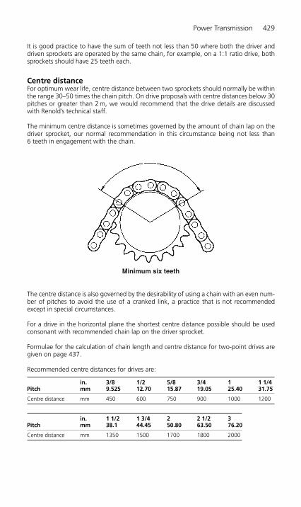
It is good practice to have the sum of teeth not less than 50 where both the driver anddriven sprockets are operated by the same chain, for example, on a 1:1 ratio drive, bothsprockets should have 25 teeth each.
Centre distanceFor optimum wear life, centre distance between two sprockets should normally be withinthe range 30–50 times the chain pitch. On drive proposals with centre distances below 30pitches or greater than 2 m, we would recommend that the drive details are discussedwith Renold’s technical staff.
The minimum centre distance is sometimes governed by the amount of chain lap on thedriver sprocket, our normal recommendation in this circumstance being not less than 6 teeth in engagement with the chain.
The centre distance is also governed by the desirability of using a chain with an even num-ber of pitches to avoid the use of a cranked link, a practice that is not recommendedexcept in special circumstances.
For a drive in the horizontal plane the shortest centre distance possible should be usedconsonant with recommended chain lap on the driver sprocket.
Formulae for the calculation of chain length and centre distance for two-point drives aregiven on page 437.
Recommended centre distances for drives are:
in. 3/8 1/2 5/8 3/4 1 1 1/4Pitch mm 9.525 12.70 15.87 19.05 25.40 31.75
Centre distance mm 450 600 750 900 1000 1200
in. 1 1/2 1 3/4 2 2 1/2 3Pitch mm 38.1 44.45 50.80 63.50 76.20
Centre distance mm 1350 1500 1700 1800 2000
Minimum six teeth
Power Transmission 429
H6508-Ch05.3.qxd 9/12/05 4:48 PM Page 429
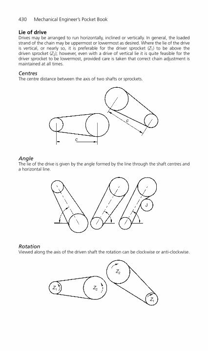
Lie of driveDrives may be arranged to run horizontally, inclined or vertically. In general, the loadedstrand of the chain may be uppermost or lowermost as desired. Where the lie of the driveis vertical, or nearly so, it is preferable for the driver sprocket (Z1) to be above the driven sprocket (Z2); however, even with a drive of vertical lie it is quite feasible for thedriver sprocket to be lowermost, provided care is taken that correct chain adjustment ismaintained at all times.
CentresThe centre distance between the axis of two shafts or sprockets.
AngleThe lie of the drive is given by the angle formed by the line through the shaft centres anda horizontal line.
RotationViewed along the axis of the driven shaft the rotation can be clockwise or anti-clockwise.
Z1
Z1
Z2
Z2
J
c
c
430 Mechanical Engineer’s Pocket Book
H6508-Ch05.3.qxd 9/12/05 4:48 PM Page 430

5.3.9 Drive layout
One chain can be used for driving a number of shafts and due to the ability of roller chainsto gear on either face, individual shafts in the same drive can be made to rotate in the sameor opposite directions by arranging the driven sprockets to gear in different faces of thechain. The number of driven sprockets permissible in any one drive depends on the layout.
A selection of possible drive layouts is shown below.
Drives with variable shaft positions
Floating countershaft and floating jockey
Chain lap: Recommended 120°. Minimum of 90° permissible for sprockets of 27 teeth or over.Centres: Pitch of chain multiplied by 30–50.
Drives with abnormally long centres
For slow and medium chain speed applications up to 150 m/min.
Or supporting jockeys
Z1
J
J
Z2
Could incorporate countershafts
Z1Z2
Z2Z2
Z1
JJZ1
�
Power Transmission 431
H6508-Ch05.3.qxd 9/12/05 4:48 PM Page 431
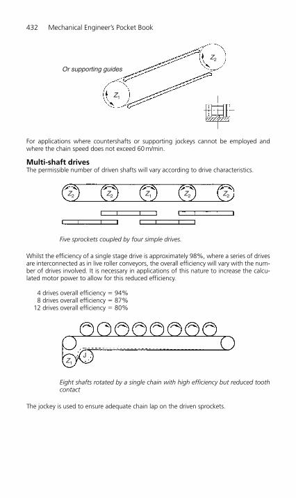
For applications where countershafts or supporting jockeys cannot be employed andwhere the chain speed does not exceed 60 m/min.
Multi-shaft drivesThe permissible number of driven shafts will vary according to drive characteristics.
Five sprockets coupled by four simple drives.
Whilst the efficiency of a single stage drive is approximately 98%, where a series of drivesare interconnected as in live roller conveyors, the overall efficiency will vary with the num-ber of drives involved. It is necessary in applications of this nature to increase the calcu-lated motor power to allow for this reduced efficiency.
4 drives overall efficiency � 94%8 drives overall efficiency � 87%
12 drives overall efficiency � 80%
Eight shafts rotated by a single chain with high efficiency but reduced toothcontact
The jockey is used to ensure adequate chain lap on the driven sprockets.
Z1
J
Z2 Z2 Z2 Z2Z1
Or supporting guides
Z1
Z2
432 Mechanical Engineer’s Pocket Book
H6508-Ch05.3.qxd 9/12/05 4:48 PM Page 432
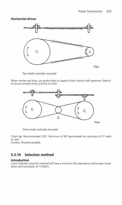
Horizontal drives
Two shafts vertically mounted
When centres are long, use guide strips to support chain strands with generous ‘lead-in’to ensure smooth entry and exit of chain.
Three shafts vertically mounted
Chain lap: Recommended 120°. Minimum of 90° permissable for sprockets of 27 teeth or over.Centres: Shortest possible.
5.3.10 Selection method
IntroductionChain selected using this method will have a minimum life expectancy with proper instal-lation and lubrication of 15 000 h.
Z2
Z1
Plan
Z2
Z2 Z1
Plan
Power Transmission 433
H6508-Ch05.3.qxd 9/12/05 4:48 PM Page 433

WarningThe rating charts pages 441 and 442 exceed the minimum standards and selection ofchain using the figures quoted in this section is only valid for Renold chain.
Use Renold’s interactive Chain Selector on www.renold.com.
Symbols, terms and unitsZ1 � number of teeth on drive sprocket.Z2 � number of teeth on driven sprocket.C � centre distance (mm).P � chain pitch (mm).i � drive ratio.L � chain length (pitches).
In order to select a chain drive the following essential information must be known:
● The power in kilowatts to be transmitted.● The speed of the driving and driven shafts.● The characteristics of the drive.● Centre distance.
From this base information, the selection power to be applied to the ratings chart isderived.
Selection summary1 Select drive ratio and sprockets Z1 � 19 teeth minimum 4342 Establish selection application factors f1 takes account of dynamic loads
Tooth factor f2 (19/Z1) 4353 Calculate selection power � power � f1 � f2 (kW) 4364 Select chain drive.
Use rating charts 437/441/4425 Calculate chain length using formulae 4376 Calculate exact centre distance 437
Finally, choose lubrication method.
Select drive and ratioChart 1 may be used to choose a ratio based on the standard sprocket sizes available. itis best to use an odd number of teeth combined with an even number of chain pitches.
Ideally, chain sprockets with a minimum of 19 teeth should be chosen. If the chain driveoperates at high speed or is subjected to impulsive loads, the smaller sprockets shouldhave at least 25 teeth and should be hardened.
It is recommended that chain sprockets should have a maximum of 114 teeth.
Drive ratio can otherwise be calculated using the formula:
For large ratio drives, check that the angle of lap of Z1 is not less than 120°.
i �Z
Z2
1
434 Mechanical Engineer’s Pocket Book
H6508-Ch05.3.qxd 9/12/05 4:48 PM Page 434

Select drive ratio and sprockets �
Chain reduction ratios to one using preferred sprockets
No. of teeth No. of teeth drive sprocket Z1driven
15 17 19 21 23 25sprocket Z2
25 – – – – – 1.0038 2.53 2.23 2.00 1.80 1.65 1.5257 3.80 3.35 3.00 2.71 2.48 2.2876 5.07 4.47 4.00 3.62 3.30 3.0495 6.33 5.59 5.00 4.52 4.13 3.80
114 7.60 6.70 6.00 5.43 4.96 4.56
For recommended centre distances see page 437
Establish selection factorsThe following factors will be used later on to determine the selection power.
Application factor f1Factor f1 takes account of any dynamic overloads depending on the chain operating con-ditions. The value of factor f1 can be chosen directly or by analogy using chart 2.
Driversprocket
Z1
Driven sprocketZ2
Centre distance
C
Z
Z2
1
120°min
Driver sprocket (Z1)
Power Transmission 435
H6508-Ch05.3.qxd 9/12/05 4:48 PM Page 435

Characteristics of driverDriven machine
Smooth running Slight shocks Moderate characteristics
Electric motors, Internal shocks steam and gas combustion Internal
turbines, internal engines with combustion combustion six cycles or engines with
engines with more with less than six hydraulic mechanical cycles with coupling coupling, electric mechanical
motors with couplingfrequent starts
Smooth Centrifugal pumps and 1 1.1 1.3running compressors, printing
machines, paper calanders, uniformly loaded conveyors, escalators, liquid agitators and mixers, rotary driers, fans
Moderate Pumps and compressors 1.4 1.5 1.7shocks (3� cycles), concrete
mixing machines, non uniformly loaded conveyors, solid agitators and mixers
Heavy Planers, excavators, roll 1.8 1.9 2.1shocks and ball mills, rubber
processing machines, presses and shears one and two cycle pumps and compressors, oil drilling rigs
Tooth factor f2The use of a tooth factor further modifies the final power selection. The choice of asmaller diameter sprocket will reduced the maximum power capable of being transmittedsince the load in the chain will be higher.
Tooth factor f2 is calculated using the formula
Note that this formula arises due to the fact that selection rating curves shown in the rat-ing charts (see pages 441 and 442) are those for a 19 tooth sprocket.
f2 factors for standard sprocket sizes
Z1 f2
15 1.2717 1.1219 1.0021 0.9123 0.8325 0.76
Calculate the selection powerMultiply the power to be transmitted by the factors obtained from step two.
Selection power � Power to be transmitted � f1 � f2 (kW).
fZ2 �19
1
436 Mechanical Engineer’s Pocket Book
H6508-Ch05.3.qxd 9/12/05 4:48 PM Page 436

This selection power can now be used with the appropriate rating chart, see pages 441and 442.
Select chain driveFrom the rating chart, select the smallest pitch of simplex chain to transmit the selectionpower at the speed of the driving sprocket Z1.
This normally results in the most economical drive selection. If the selection power is nowgreater than that shown for the simplex chain, then consider a multiplex chain of thesame pitch size as detailed in the ratings chart.
Calculate chain lengthTo find the chain length in pitches (L) for any contemplated centre distance of a two pointdrive, use the formula below:
The calculated number of pitches should be rounded up to a whole number of evenpitches. Odd numbers of pitches should be avoided because this would involve the use ofa cranked link which is not recommended. If a jockey sprocket is used for adjustment pur-poses, two pitches should be added to the chain length (L).
C is the contemplated centre distance in mm and should generally be between 30 and 50pitches.
For example, for 1 in. pitch chain C � 1.5 � 25.4 � 40 � 1524 mm.
Calculate exact centre distanceThe actual centre distance for the chain length (L) calculated by the method above, will ingeneral be greater than that originally contemplated. The revised centre distance can becalculated from the formula below.
where:P � chain pitch (mm)L � chain length (pitches)Z1 � number of teeth in driver sprocketZ2 � number of teeth in driven sprocket
Drive with multiple sprocketsWhen designing a drive with multiple sprockets, the chain length calculation becomesmore complicated. Most CAD systems, however, can be used to calculate chain length by
CP
L Z Z L Z Z Z Z� � � � � � � �8
2 2 212 1 2 1 2
2
3.88( )( )
p⎛
⎝⎜⎜⎜⎜⎜
⎞
⎠⎟⎟⎟⎟⎟
⎡
⎣
⎢⎢⎢⎢
⎤
⎦
⎥⎥⎥⎥
12
Length ( )2
2P
21 2
2 1
LZ Z
��
� �
�
C
Z Z
p
⎛
⎝⎜⎜⎜⎜⎜
⎞
⎠
⎟⎟⎟⎟⎟
22
� P
C
Power Transmission 437
H6508-Ch05.3.qxd 9/12/05 4:48 PM Page 437
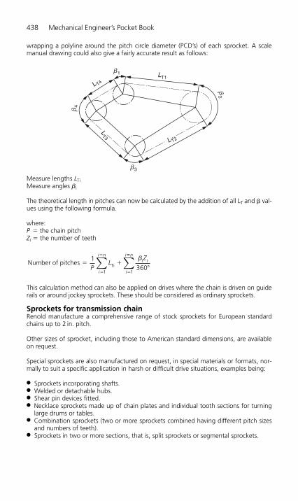
wrapping a polyline around the pitch circle diameter (PCD’s) of each sprocket. A scalemanual drawing could also give a fairly accurate result as follows:
Measure lengths LTiMeasure angles �i
The theoretical length in pitches can now be calculated by the addition of all LT and � val-ues using the following formula.
where:P � the chain pitchZi � the number of teeth
This calculation method can also be applied on drives where the chain is driven on guiderails or around jockey sprockets. These should be considered as ordinary sprockets.
Sprockets for transmission chainRenold manufacture a comprehensive range of stock sprockets for European standardchains up to 2 in. pitch.
Other sizes of sprocket, including those to American standard dimensions, are availableon request.
Special sprockets are also manufactured on request, in special materials or formats, nor-mally to suit a specific application in harsh or difficult drive situations, examples being:
● Sprockets incorporating shafts.● Welded or detachable hubs.● Shear pin devices fitted.● Necklace sprockets made up of chain plates and individual tooth sections for turning
large drums or tables.● Combination sprockets (two or more sprockets combined having different pitch sizes
and numbers of teeth).● Sprockets in two or more sections, that is, split sprockets or segmental sprockets.
Number of pitches1
360Ti1
i i� ��
�
�
�P
LZ
i
i n
i
i
∑ b
1
��n
∑
L T4
LT1b1
b3
b2
b4
LT3
L T2
438 Mechanical Engineer’s Pocket Book
H6508-Ch05.3.qxd 9/12/05 4:48 PM Page 438
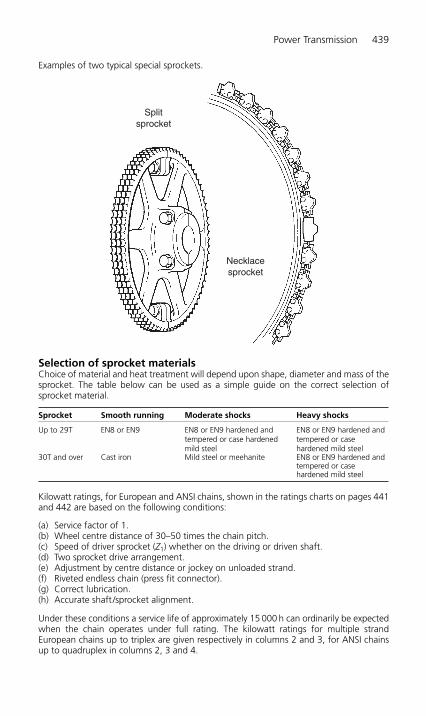
Examples of two typical special sprockets.
Selection of sprocket materialsChoice of material and heat treatment will depend upon shape, diameter and mass of thesprocket. The table below can be used as a simple guide on the correct selection ofsprocket material.
Sprocket Smooth running Moderate shocks Heavy shocks
Up to 29T EN8 or EN9 EN8 or EN9 hardened and EN8 or EN9 hardened and tempered or case hardened tempered or case mild steel hardened mild steel
30T and over Cast iron Mild steel or meehanite EN8 or EN9 hardened and tempered or case hardened mild steel
Kilowatt ratings, for European and ANSI chains, shown in the ratings charts on pages 441and 442 are based on the following conditions:
(a) Service factor of 1.(b) Wheel centre distance of 30–50 times the chain pitch.(c) Speed of driver sprocket (Z1) whether on the driving or driven shaft.(d) Two sprocket drive arrangement.(e) Adjustment by centre distance or jockey on unloaded strand.(f) Riveted endless chain (press fit connector).(g) Correct lubrication.(h) Accurate shaft /sprocket alignment.
Under these conditions a service life of approximately 15 000 h can ordinarily be expectedwhen the chain operates under full rating. The kilowatt ratings for multiple strandEuropean chains up to triplex are given respectively in columns 2 and 3, for ANSI chainsup to quadruplex in columns 2, 3 and 4.
Splitsprocket
Necklacesprocket
Power Transmission 439
H6508-Ch05.3.qxd 9/12/05 4:48 PM Page 439

5.3.11 Rating chart construction
The rating charts at first sight look complicated, however, they are constructed from threesimple lines. From this it may be seen that at lower speeds the failure mode is likely to beplate fatigue if the maximum power recommendation is exceeded. However, pin gallingwill occur due to boundary lubrication break down at very high speeds. At the intersec-tion of these lines the bush and roller fatigue curve comes into a play and accounts forthe rounded tops to each of the selection curves.
Bearing pressuresWhen a chain has been correctly selected, the mode of failure over a very long period oftime is most likely to be wear.
The subject of wear, which depends on many factors, has been addressed earlier in thisguide, however, a very useful indicator of the likely wear performance is the magnitudeof pressure between the key mating surfaces, that is, pin and bush.
This pressure is known as the bearing pressure, and is obtained by dividing the workingload by the bearing area. Bearing areas for standard chains are quoted in the designerdata at the end of this guide.
The following table gives an indication of the implications of various bearing pressuresbut should not be used without reference to the other chain selection methods given inthis guide.
80
Sim
plex
Sim
ple
Sim
ple
Mul
tiple
x
Mul
tiple
x
Mul
tiple
x
60
40
20
Contact Renold
Reduced life
Good lifeexpectancy
Slow HighMedium
Chain velocity (m/s)
Bea
ring
pres
sure
(N
/mm
2 )
Rating chart construction
Speed
Bush and rollerfatigue
Pin gallingLink plate fatigue
Pow
er
440 Mechanical Engineer’s Pocket Book
H6508-Ch05.3.qxd 9/12/05 4:48 PM Page 440
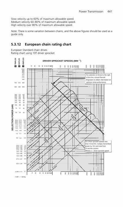
Slow velocity up to 60% of maximum allowable speed.Medium velocity 60–80% of maximum allowable speed.High velocity over 80% of maximum allowable speed.
Note: There is some variation between chains, and the above figures should be used as aguide only.
5.3.12 European chain rating chart
European Standard chain drivesRating chart using 19T driver sprocket
For selection of drives to the right
of this line, consult Renold
Engineers to obtain information on
optimum drive performance.
DRIVER SPROCKET SPEEDS (MIN�1)
15
1000900800700600
500
400
300510750
340500 200
170250 100153225 90
5175 30
3450 20
17.025.0 10.015.322.5 9.0
8.512.5 5.0
6.810.0 4.0
5.17.5 3.0
3.45.0 2.0
1.702.50 1.0
1.021.50 0.6
0.851.25 0.5
0.681.00 0.4
0.510.75 0.3
0.340.50 0.2
0.170.250
1 kW � 1.34 hp.
0.1
1.191.75 0.71.362.00 0.81.532.25 0.9
10.215.0 6.011.917.5 7.013.620.0 8.0
68100 40
85125 50
102150 60119175 70136200 80
20 30 40 50 60 70 80 90 100
200
300
400
500
600
700
800
900
1000
2000
3000
4000
5000
6000
7000
8000
9000
1000
0
15 20 30 40 50 60 70 80 90 200
300
400
500
600
700
800
900
2000
3000
4000
5000
6000
7000
8000
9000
For driver sprocket speeds lessthan 10 rev/min, multiply transmittedpower by 10/n and read from10 rev/min column.Where n � driver sprocket speed.
TR
IPL
EX
DU
PL
EX
SIM
PL
EX
8"mm pitc
h
3/8" (9,525 mm) p
itch
1/2" (12,70 mm) p
itch
5/8" (15,875 mm) p
itch
3/4" (19,05 mm) p
itch
1" (25,40 mm) p
itch
11/4" (3
1,75 mm) pitc
h11/2"
(38,10 mm) p
itch
13/4" (4
4,45 mm) pitc
h
2" (50,80 mm) p
itch
21/2" (6
3,50 mm) pitc
h3" (76,20 mm) p
itch
SE
LE
CT
ION
PO
WE
R (
kW) OIL STREAM
TYPE 4
OIL BATH
TYPE 3
DRIP FEED
TYPE 2
MANUAL
TYPE 1
3 2 1
Power Transmission 441
H6508-Ch05.3.qxd 9/12/05 4:48 PM Page 441
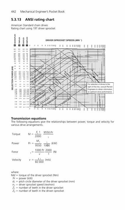
5.3.13 ANSI rating chart
American Standard chain drivesRating chart using 19T driver sprocket
Transmission equationsThe following equations give the relationships between power, torque and velocity forvarious drive arrangements.
where:Md � torque of the driver sprocket (Nm)
Pr � power (kW)d1 � pitch circle diameter of the driver sprocket (mm)n1 � driver sprocket speed (rev/min)Z1 � number of teeth in the driver sprocketZ2 � number of teeth in the driven sprocket
Torque M1
20009550.Pr
Power Pr9550 10
1
1 1
�
�
F
M1
000(kW)
Force1000 Pr
N
Velocity
1 �
�
v
v
20001
( )
11 1
60 000m/s( )
DRIVER SPROCKET SPEEDS (MIN�1)
10 15 20 30 40 50 60 70 80 90 100
150
200
300
400
500
600
700
800
900
1000
1500
2000
3000
4000
5000
6000
7000
8000
9000
1000
0
For selection of drives to theright of this line, consult RenoldEngineers to obtain informationon optimum drive performance.
10 15 20 30 40 50 60 70 80 90 100
150
200
300
400
500
600
700
800
900
1000
1500
2000
3000
4000
5000
6000
7000
8000
9000
1000
0
660
495
330297264231198165132
99
66
50
33.029.726.423.119.816.513.2
9.9
6.6
5.0
SE
LE
CT
ION
PO
WE
R (
kW)
25.022.520.017.515.012.510.0
7.5
5.0
3.8
2.502.252.001.751.501.251.00
0.75
0.50
0.38
0.250.33
0.50
0.66
0.99
1.321.611.982.312.642.973.30
17.015.313.611.910.2
8.56.8
9.08.07.06.05.04.0
5.1 3.0
2.0
1.5
3.4
2.6
1.70 1.000.900.800.700.600.500.40
0.30
0.20
0.15
0.100.17
0.26
0.34
0.51
0.68
1.531.361.191.020.85
10.0
375
250225200175150125100
75
50
38
255
170153136119102
8568
51
34
26
150
100908070605040
40
20
15
500 340 200
QU
AD
UP
LE
X
TR
IPL
EX
DU
PL
EX
SIM
PL
EX
4 3 2 1
1/4" (6,35 mm) p
itch
3/8" (9,525 mm) p
itch
1/2" (12,70 mm) p
itch
5/8" (15,875 mm) p
itch
3/4" (19,05 mm) p
itch
1" (25,40 mm) p
itch
11/4" (31,75mm) p
itch
11/2" (38,10 mm) p
itch
13/4" (44,45 mm) p
itch
2" (50,80 mm) p
itch
21/2" (63,50 mm) p
itch
OIL STREAM
TYPE 4
OIL BATHTYPE 3
DRIP FEED
TYPE 2
MANUALTYPE 1
442 Mechanical Engineer’s Pocket Book
H6508-Ch05.3.qxd 9/12/05 4:48 PM Page 442

v � linear speed of the chain (m/s)F1 � chain pull (N)P � pitch of the chain (mm)
Centripetal accelerationCentripetal acceleration affecting parts of the chain engaged on the sprockets is deter-mined by:
F2 � q �v2 (N)
where:F2 � force (N)q � mass of the chain (kg/m)
From this formula we can see that at high speed, this force is not negligible and is themain reason for speed limitation.
5.3.14 Chain suspension force
The force acting between one link and the next due to the mass of the chain is small andis internally balanced within the chain. This will do no more than cause the chain to adopta sagging catenery shape between the sprockets.
Allowance will need to be made in the installation for the slightly different posturesadopted by the chain between zero and maximum load.
5.3.15 Lubrication
Chain drives should be protected against dirt and moisture and be lubricated with goodquality non-detergent mineral based oil. A periodic change of oil is desirable. Heavy oilsand greases are generally too stiff to enter the chain working surfaces and should not be used.
Care must be taken to ensure that the lubricant reaches the bearing areas of the chain.This can be done by directing the oil into the clearances between the inner and outer linkplates, preferably at the point where the chain enters the sprocket on the bottom strand.
The table below indicates the correct lubricant viscosity for various ambient temperatures.
Ambient temperature Lubricant rating
°C SAE BS 4231
�5 to �5 20 46 to 685 to 40 30 100
40 to 50 40 150 to 22050 to 60 50 320
For the majority of applications in the above temperature range, a multigrade SAE 20/50oil would be suitable.
Power Transmission 443
H6508-Ch05.3.qxd 9/12/05 4:48 PM Page 443
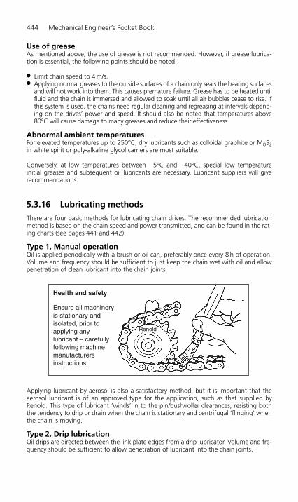
Use of greaseAs mentioned above, the use of grease is not recommended. However, if grease lubrica-tion is essential, the following points should be noted:
● Limit chain speed to 4 m/s.● Applying normal greases to the outside surfaces of a chain only seals the bearing surfaces
and will not work into them. This causes premature failure. Grease has to be heated untilfluid and the chain is immersed and allowed to soak until all air bubbles cease to rise. Ifthis system is used, the chains need regular cleaning and regreasing at intervals depend-ing on the drives’ power and speed. It should also be noted that temperatures above80°C will cause damage to many greases and reduce their effectiveness.
Abnormal ambient temperaturesFor elevated temperatures up to 250°C, dry lubricants such as colloidal graphite or MOS2in white spirit or poly-alkaline glycol carriers are most suitable.
Conversely, at low temperatures between �5°C and �40°C, special low temperature initial greases and subsequent oil lubricants are necessary. Lubricant suppliers will giverecommendations.
5.3.16 Lubricating methods
There are four basic methods for lubricating chain drives. The recommended lubricationmethod is based on the chain speed and power transmitted, and can be found in the rat-ing charts (see pages 441 and 442).
Type 1, Manual operationOil is applied periodically with a brush or oil can, preferably once every 8 h of operation.Volume and frequency should be sufficient to just keep the chain wet with oil and allowpenetration of clean lubricant into the chain joints.
Applying lubricant by aerosol is also a satisfactory method, but it is important that theaerosol lubricant is of an approved type for the application, such as that supplied byRenold. This type of lubricant ‘winds’ in to the pin/bush/roller clearances, resisting boththe tendency to drip or drain when the chain is stationary and centrifugal ‘flinging’ whenthe chain is moving.
Type 2, Drip lubricationOil drips are directed between the link plate edges from a drip lubricator. Volume and fre-quency should be sufficient to allow penetration of lubricant into the chain joints.
Health and safety
Ensure all machineryis stationary andisolated, prior toapplying anylubricant – carefullyfollowing machinemanufacturersinstructions.
Renold
444 Mechanical Engineer’s Pocket Book
H6508-Ch05.3.qxd 9/12/05 4:48 PM Page 444

Type 3, Bath or disc lubricationWith oil bath lubrication the lower strand of chain runs through a sump of oil in the drivehousing. The oil level should cover the chain at its lowest point whilst operating.
With slinger disc lubrication an oil bath is used, but the chain operates above the oil level.A disc picks up oil from the sump and deposits it on the chain by means of deflectionplates. When such discs are employed they should be designed to have peripheral speedsbetween 180 and 2440 m/min.
Type 4, Stream lubricationA continuous supply of oil from a circulating pump or central lubricating system isdirected onto the chain. It is important to ensure that the spray holes from which the oilemerges are in line with the chain edges. The spray pipe should be positioned so that theoil is delivered onto the chain just before it engages with the driver sprocket.
Oil feedto chain
Spray pipe
Power Transmission 445
H6508-Ch05.3.qxd 9/12/05 4:48 PM Page 445

This ensures that the lubricant is centrifuged through the chain and assists in cushioningroller impact on the sprocket teeth. Stream lubrication also provides effective cooling andimpact damping at high speeds.
Effect of temperatureAn important factor to control in a drive system is the chain and chaincase temperaturesduring operation. Depending on the severity of the drive service, continuity of use, etc.,special attention to the lubrication method may be required.
Chain temperatures above 100°C should be avoided if possible due to lubrication limita-tions, although chain can generally give acceptable performance up to around 250°C insome circumstances. A way of improving the effectiveness of the lubrication and its cool-ing effect is to increase the oil volume (up to 4.5 l/min per chain strand) and incorporatea method of external cooling for the oil.
5.3.17 Lifting applications
This section covers applications, such as lifting and moving, where the loads involved aregenerally static. Obviously, dynamic loads are also involved in most applications and thedesigner needs to take due consideration of these. The machinery designer should alsorefer to DTI Publication INDY J1898 40 M which summarises legislation in place from 1st January 1993 to 1st January 1995 regarding machinery product standards.
Chain for lifting applications falls into two main categories:
● Leaf chains.● Bush and roller chains.
Leaf chainLeaf chain is generally used for load balancing type lifting applications as illustratedbelow. They must be anchored at either end since there is no means of geared engage-ment in the chain itself.
Safety factorsA safety factor of 7:1 is normal for steady duty reciprocating motion, for example, fork lifttrucks. For medium shock loads, 9:1 and for heavy shock loads, 11:1.
Operating speedApplications should not exceed a maximum chain speed of 30 m/min.
446 Mechanical Engineer’s Pocket Book
H6508-Ch05.3.qxd 9/12/05 4:48 PM Page 446

Applications1. Machine tools – planers, drills, milling heads, machine centres.2. Fork lift trucks, lifts, hoists.3. Counterweight balances – jacks, doors, gates, etc.
Bush and Roller chainsBush and roller chains can be used for lifting and moving purposes, and have the advan-tage over leaf chain in that they may be geared into a suitable driving sprocket. Rollerchain has a better wear resistance than leaf chain and may be used at higher speeds.
Safety factorsApplications vary widely in the nature of loads applied and it is therefore recommendedthat factors of safety are applied which allow for some degree of abuse:
● A factor of safety of 8:1 in non-passenger applications.● A factor of safety of 10:1 in passenger applications.
Lower factors of safety than these may be used (except for passenger applications), wherecareful consideration of the maximum loads and health and safety implications have beenmade. For comments on this see the section ‘Influences on chain life’.
Operating speedsApplications should not normally exceed a maximum chain speed of 45 m/min. Forspeeds higher than this, consider selection as if the chain were in a power transmissionapplication converting the chain load to power using the following formula:
Power � FV (kW)
where:F � Load (kN)V � Velocity of chain (m/s)
Then apply selection power factors as shown in step two of ‘Drive Selection’.
Calculate equivalent rev/min by using the smallest sprocket in the system where
speed �
where:P � Chain pitch (mm)Z � No of teeth in sprocket
Select lubrication methods also from the selection chart.
60 000 VPZ
Power Transmission 447
H6508-Ch05.3.qxd 9/12/05 4:48 PM Page 447

5.3.18 ANSI Xtra range
Transmission chain is also available in heavy duty versions of the ANSI standard range ofchain.
These chains are suitable where frequent or impulsive load reversals are involved. Typicalapplications are in primary industries, such as mining, quarrying, rock drilling, forestry andconstruction machinery.
In order to accommodate these higher fatigue inducing loads, material for inner andouter plates is increased in thickness by approximately 20%.
This modification does not improve the tensile strength since the pin then becomes theweakest component. However, heavy duty chains with higher tensile strength are avail-able. This is achieved by through hardening instead of case hardening the pin, but unfor-tunately this action reduces wear performance due to the lower pin hardness.
Renold ANSI Xtra chains are available as follows:
● Xtra H range Thicker plates● Xtra V range Through hardened pins● Xtra HV range Thicker plates and through hardened pins.
The H and HV chains are not suitable or appropriate for high speed transmission applications.
The following points should also be noted:
● The V range of chains are totally interchangeable with standard ANSI chain.● Simple chains of standard, H or HV designs all have identical gearing dimensions and
therefore can operate on the same sprockets as for standard chains. The thicker plateswill require a larger chain track and it may be desirable to use sprockets with heattreated teeth. Multiplex chain requires an increased transverse pitch of the teeth butother gearing dimensions are the same.
● The only reason to use H or HV chains is where fatigue life is a problem. We do notmake any cranked (offset) links or slip-fit connecting links for this range, since thesehave a lower fatigue resistance.
● Detachable (cottered) versions can be produced if required as could triplex or widerchains.
5.3.19 Influences on chain life
Factors of safetyAll Renold chain is specified by its minimum tensile strength. To obtain a design workingload it is necessary to apply a ‘factor of safety’ to the breaking load. However, before con-sidering this, the following points should be noted:
● Most chain side plates are manufactured from low to medium carbon steel and aresized to ensure they have adequate strength and also ductility to resist shock loading.
● These steels have yield strengths around 65% of their ultimate tensile strength. Whatthis means is that if chains are subjected to loads of greater than this, depending onthe material used in the side plates, then permanent pitch extension will occur.
● Most applications are subjected to transient dynamic loads well in excess of the max-imum static load and usually greater than the designer’s estimate.
448 Mechanical Engineer’s Pocket Book
H6508-Ch05.3.qxd 9/12/05 4:48 PM Page 448

● Motors, for example, are capable of up to 200% full load torque output for a shortperiod.
The consequences of these points are that chain confidently selected with a factor of safetyof 8:1 on breaking load is, in effect, operating with a factor of safety of around 5:1 on yieldand much less than this when the instantaneous overload on the drive is considered.
A further consideration when applying a factor of safety to a chain application is therequired chain life.
In a properly maintained application a life of 8 000 000 cycles or 15 000 h, whichevercomes first, is normal. Wear will be the usual mode of failure.
In applications where low factors of safety are required, the life will reduce accordingly.
The maximum working load is obtained by dividing the chain minimum tensile strengthby the factor of safety.
The table below gives a rough indication of life for various factors of safety.
Factor Cycles maximum Type of application
Simple Multiplex
5.0 6.0 1 000 000 Dynamic load does not exceed working load6.0 7.2 2 000 0008.0 8.0 8 000 000 Dynamic loads can occasionally exceed working
load by 20%10.0 10.0 8 000 000 All passenger lifts
Safety factors
Harsh environments
passenger lifts
Transmission
High cycle lifting
Low cycle lifting
Not normally usedAxi
al b
reak
ing
forc
e/m
axim
um w
orki
ng lo
ad
Saf
ety
criti
cal
12
11
10
9
8
7
6
5
4321
Power Transmission 449
H6508-Ch05.3.qxd 9/12/05 4:48 PM Page 449
It should be noted that at factors below 8:1, bearing pressures increase above the max-imum recommended, with the result that increased wear will arise unless special attentionis taken with lubrication, for example:
● More frequent lubrication.● Higher performance lubricants.● Better methods of applying lubrication.
Important noteFor factors of 5:1 the resulting bearing pressure is 50% higher than recommended andchain working under these conditions will wear prematurely, whatever type of lubricationregime is used.
Harsh environmentsIn anything other than a clean and well lubricated environment, the factor of safetyshould be adjusted if some detriment to the working life of the chain is to be avoided.Low temperatures will also decrease working life, especially if shock loads are involved.
The following tables give a general guide to the appropriate safety factors for differentapplications for a target life of 8 000 000 cycles.
Cleanliness
Lubrication Clean Moderately clean Dirty/abrasive
Regular 8 10 12Occasional 10 12 14None 12 12 14
Temperature (°C)
Lubrication �10 to 150 150 to 200 200 to 300
Regular 8 10 12Occasional 10 12 14None 12 12 14
Load regime
Temperature (°C) Smooth Moderate shocks Heavy shocks
�10 to �150 8 11 150 to �10 10 15 19�20 to 0 12 20 25�40 to �20 15 25 33
5.3.20 Chain extension
When designing lifting applications it can be useful to know how much a chain willextend under a given load.
The approximate elongation of a chain under a given load can be measured by using thefollowing formulae:
● Simplex Chain
● Duplex Chain �� ��
LL
PF
(9.72) 10 5
2 1
�� ��
LL
PF
(14.51) 10 5
2 1
450 Mechanical Engineer’s Pocket Book
H6508-Ch05.3.qxd 9/12/05 4:48 PM Page 450
● Triplex Chain
where:L � change in chain length (mm)
L � original length of the chain (mm)P � pitch of the chain (mm)
F1 � average load in the chain.
5.3.21 Matching of chain
Any application in which two or more strands of transmission chain are required to operateside by side in a common drive, or conveying arrangement, may involve the need for eitherpairing or matching. Such applications generally fall into one of the following categories:
Length matching for conveying and similar applicationsWherever length matching of transmission chain is necessary it is dealt with as follows:
● The chains are accurately measured in handling lengths between 3 m and 8 m asappropriate and then selected to provide a two (or more) strand drive having overalllength uniformity within close limits. However, such length uniformity will not neces-sarily apply to any intermediate sections along the chains, but the actual length of allintermediate sections, both along and across the drive, will not vary more than our nor-mal manufacturing limits. However, adapted transmission chains are usually manufac-tured to specific orders which are generally completed in one production run so that itis reasonable to assume that length differences of intermediate sections will be small.
● Chains are supplied in sets which are uniform in overall length within reasonably finelimits and will be within our normal manufacturing limits. It should be noted that chainsets supplied against different orders at different times may not have exactly the samelengths to those supplied originally, but will vary by no more than our normal toleranceof 0.0%, �0.15%.
Pitch matching transmission drive chainsPitch matched chains are built up from shorter subsections (usually 300 to 600 mmlengths) which are first measured and then graded for length. All subsections in eachgrade are of closely similar length and those forming any one group across the set ofchains are selected from the same length grade.
The requisite number of groups are then connected to form a pitch matched set ofchains, or alternatively, if this is too long for convenient handling, a set of handling sec-tions for customer to assemble as a final set of pitch matched chain. Suitable tags arefixed to the chains to ensure they are connected together in the correct sequence.
Identification of handling lengths
Handling lengths
1 2 3
A strand A–A1 A1–A2 A2–A3B strand B–B1 B1–B2 B2–B3C strand C–C1 C1–C2 C2–C3
Long chains are made up in sections, each section being numbered on end links. Sectionsshould be so joined up that end links with similar numbers are connected. Where chainsare to run in sets of two or more strands, each strand is stamped on end links of each
�� ��
LL
PF
(7.26) 10 5
2 1
Power Transmission 451
H6508-Ch05.3.qxd 9/12/05 4:48 PM Page 451

section with a letter, in addition to being numbered. Correct consecutive sections for eachstrand must be identified from the end links and joined up as indicated.
By these means, the actual length of any intermediate portion of one strand (as measuredfrom any one pitch point to any other) will correspond closely with that of the transverselyequivalent portion on the other strands, generally within 0.05 mm, depending on thechain pitch size.
Pitch matching adapted transmission chains (when attachments are fitted to chains)With the sole exception of extended bearing pins, it is not possible to match the pitch ofholes in attachments themselves to within very fine limits, due to the additional tolerancesto be contended with (bending, holing, etc.).
Colour codingFor customers who wish to match their chains, perhaps in order to fit special attachmentsin situ, Renold colour code short lengths of chain within specified tolerance bands. Thesewill normally be red, yellow or green paint marks to indicate lower, mid and upper thirdsof the tolerance band. For even finer tolerance bands additional colours can be used, butnormally a maximum of five colours will be more than adequate.
Colour Red 0.05%Yellow 0.10%Green 0.15%Blue For finerWhite Tolerances
5.3.22 To measure chain wear
A direct measure of chain wear is the extension in excess of the nominal length of thechain. the chain wear can therefore be ascertained by length measurement in line withthe instructions given below:
● Lay the chain, which should terminate at both ends with an inner link (part No 4), ona flat surface, and, after anchoring it at one end, attach to the other end a turnbuckleand a spring balance suitably anchored.
● Apply a tension load by means of the turnbuckle amounting to:
Simplex chain P2 � 0.77 (N)Duplex chain P2 � 1.56 (N)Triplex chain P2 � 2.33 (N)
where P is the pitch in mm.
In the case of double pitch chains (e.g. chains having the same breaking load and twicethe pitch) apply measuring loads as for the equivalent short pitch chains.
As an alternative, the chain may be hung vertically and the equivalent weight attached tothe lower end.
M
452 Mechanical Engineer’s Pocket Book
H6508-Ch05.3.qxd 9/12/05 4:48 PM Page 452
● Measure length ‘M’ (see diagram above) in millimetres from which the percentageextension can be obtained from the following formula:
where:N � Number of pitches measuredP � Pitch
● As a general rule, the useful life of the chain is terminated and the chain should bereplaced when extension reaches 2% (1% in the case of double pitch chains). Fordrives with no provision for adjustment, the rejection limit is lower, dependent on thespeed and layout. A usual figure is between 0.7% and 1.0% extension.
Renold chain wear guideA simple-to-use chain wear guide is available from Renold chain for most popular sizes ofchain pitch. Please contact your Sales Office for details.
5.3.23 Repair and replacement
SprocketsExamination of both flanks will give an indication of the amount of wear which hasoccurred. Under normal circumstances this will be evident as a polished worn strip aboutthe pitch circle diameter of the sprocket tooth.
If the depth of this wear ‘X’ has reached an amount equal to 10% of the ‘Y’ dimension,then steps should be taken to replace the sprocket. Running new chain on sprockets hav-ing this amount of tooth wear will cause rapid chain wear.
It should be noted that in normal operating conditions, with correct lubrication theamount of wear ‘X’ will not occur until several chains have been used.
ChainChain repair should not as a rule be necessary. A correctly selected and maintained chainshould gradually wear out over a period of time (approximately 15 000 h), but it shouldnot fail. Please refer to the Installation and Maintenance section, which gives an indica-tion of the service life remaining.
If a transmission chain sustains damage due to an overload, jam-up, or by riding over thesprocket teeth, it should be carefully removed from the drive and given a thorough visualexamination. Remove the lubricating grease and oil to make the job easier.
Depending on the damage, it may be practicable to effect temporary repairs usingreplacement links. However, it is not a guarantee that the chain has not been over
Depthof wear
PCDPCD X
X �
Y
Y10
Percentage extension M(N )N
100� ��
��
PP
Power Transmission 453
H6508-Ch05.3.qxd 9/12/05 4:48 PM Page 453

stressed and so made vulnerable to a future failure. The best policy, therefore, is toremove the source of trouble and fit a new chain. This should be done for the followingreasons:
1. The cost of down time to the system or machine can often outweigh the cost ofreplacing the chain.
2. A new or even used portion of chain or joints assembled into the failed chain willcause whipping and load pulsation. This can, and probably will, produce rapid failureof the chain and will accelerate wear in both the chain and its sprockets.
If a chain has failed two or more times, it is certain the chain will fail again in time. If no replacement is immediately available, repair the chain, but replace it at the earliestopportunity.
5.3.24 Chain adjustment
To obtain full chain life, some form of chain adjustment must be provided, preferably bymoving one of the shafts. If shaft movement is not possible, an adjustable jockey sprocketengaging with the unloaded strand of the chain is recommended. Generally the jockeyshould have the same number of teeth as the driver sprocket and care should be taken toensure the speed does not exceed the maximum shown in the rating charts (see pages437 and 438).
The chain should be adjusted regularly so that, with one strand tight, the slack strand canbe moved a distance ‘A’ at the mid point (see diagram below). To cater for any eccentri-cities of mounting, the adjustment of the chain should be tried through a complete revo-lution of the large sprocket.
A � total movement
C � horizontal centre distance
Total movement ‘A’ (mm) �
where:K � 25 for smooth drives
50 for shock drives
For vertical drives please consult the installation and maintenance section, which givesmore details on chain adjustment.
C
A
CK(mm)
454 Mechanical Engineer’s Pocket Book
H6508-Ch05.3.qxd 9/12/05 4:48 PM Page 454
5.3.25 Design ideas
A variety of applications.
Conveying, indexing, lifting and pulling, power transmission and timing.
Power Transmission 455
H6508-Ch05.3.qxd 9/12/05 4:48 PM Page 455
A variety of industries.
Aircraft, automotive, marine, mechanical handling, motorcycle, nuclear oilfield.
456 Mechanical Engineer’s Pocket Book
H6508-Ch05.3.qxd 9/12/05 4:48 PM Page 456

5.3.26 Table of PCD factors
To obtain PCD of any sprocket with 9 to 150 teeth, multiply chain pitch by appropriatefactor.
For example, the PCD of a 38T sprocket of 3/4 in. (19.05 mm) pitch � 19.05 � 12.110 �230.70 mm.
Power Transmission 457
9 2.92410 3.23611 3.54912 3.86413 4.17914 4.49415 4.81016 5.12617 5.44218 5.75919 6.07620 6.39221 6.70922 7.02723 7.34424 7.66125 7.97926 8.29627 8.61428 8.93129 9.24930 9.56731 9.88532 10.20233 10.52034 10.83835 11.15636 11.47437 11.79238 12.11039 12.42840 12.74641 13.06342 13.38243 13.70044 14.01845 14.33646 14.65447 14.97248 15.29049 15.60850 15.92651 16.24452 16.56253 16.88054 17.19855 17.51756 17.835
57 18.15358 18.47159 18.78960 19.10761 19.42662 19.74463 20.06264 20.38065 20.69866 21.01667 21.33568 21.65369 21.97170 22.28971 22.60772 22.92673 23.24474 23.56275 23.88076 24.19877 24.51778 24.83579 25.15380 25.47181 25.79082 26.10883 26.42684 26.74485 27.06386 27.38187 27.69988 28.01789 28.33590 28.65491 28.97292 29.29093 29.60894 29.92795 30.24596 30.56397 30.88198 31.20099 31.518
100 31.836101 32.154102 32.473103 32.791104 33.109
105 33.428106 33.746107 34.064108 34.382109 34.701110 35.019111 35.337112 35.655113 35.974114 36.292115 36.610116 36.928117 37.247118 37.565119 37.883120 38.202121 38.520122 38.838123 39.156124 39.475125 39.793126 40.111127 40.429128 40.748129 41.066130 41.384131 41.703132 42.021133 42.339134 42.657135 42.976136 43.294137 43.612138 43.931139 44.249140 44.567141 44.885142 45.204143 45.522144 45.840145 46.159146 46.477147 46.795148 47.113149 47.432150 47.750
No. of teeth PCD factor No. of teeth PCD factor No. of teeth PCD factor
H6508-Ch05.3.qxd 9/12/05 4:48 PM Page 457

5.3.27 Simple point to point drives: Example one
The following worked examples give simple step-by-step guidance on selecting varioustypes of chain drive systems. Renold technical staff are available to advise on any chainselection problems.
For details of transmission equations see page 442.
Example one: Rotary pump driveGiven:
● Pump speed 360 rev/min● Power absorbed 7.5 kW● Driver Electric motor at 1440 rev/min● Constraints Centre distance approximately 458 mm
Adjustment by shaft movement
Selection parameters● Use Z1 � 19T● No polygonal effect● Satisfactory for smooth drives
Calculate the drive ratio as follows:
Therefore the driven number of teeth
Z2 � 4 � Z1 � 4 �19 � 76T
Selection factorsApplication factor f1 � 1 (driver and driven sprockets smooth running):
Tooth factor
Selection power � 7.5 � 1 � 1 � 7.5 kW
Select chainThe chain can now be selected using charts 3 and 4 and cross referencing power tospeed, giving the following possibilities:
0.5 BS Simplex (approximately 81% of rated capacity)0.375 BS Duplex (approximately 98% of rated capacity)0.5 ANSI Simplex (approximately 83% of rated capacity)0.375 ANSI Duplex (approximately 84% of rated capacity)
0.375 ANSI Duplex chain is unsuitable as it is a bush chain.
Note: The approximation percentage of rated capacity is calculated by dividing the selec-tion power at 1440 rev/min by the chains maximum capacity at 1440 rev/min.
For this example we will choose 0.5 European Simplex.
fZ219 19
191� � �
1
Drive ratio iZ
Z
N
N� � � � �2
1
2
1
1440360
4
458 Mechanical Engineer’s Pocket Book
H6508-Ch05.3.qxd 9/12/05 4:48 PM Page 458

Installation parametersLubrication European chain rating chart (see page 441) clearly indicates the chainneeds oilbath lubrication. The chain will need to be enclosed and run in a sump of oil.
We now calculate the chain length:
Round up to the nearest number of even pitches, that is, 122.
Centre distance calculationThe centre distance of the drive can now be calculated using the formula shown below:
� 458.6 mm
AdjustmentProvide for chain wear of 2% or two pitches, whichever is smaller, in this case,(122 � 1.02) � 122 � 2.44 pitches.
Therefore use two pitches and recalculate using:
L � 124 in the above equation. This givesC � 471.7 mm
that is, total adjustment of 13.1 mm.
Note that in practice, some negative adjustment will facilitate assembly and will be essen-tial if it is intended to assemble chain which is pre-joined into an endless loop.
Other data
Chain velocity N P Z� �
�� �
�1
60 600001440 12.7 19
0005.79 m/s
� � � � � � � � �12.7
8122 76 19 2 122 76 19
3.82
2( )( ) ( )( ) �
8876 19� �( )
⎡
⎣
⎢⎢⎢
⎤
⎦
⎥⎥⎥
2
� � � � � � � �P
L Z Z L Z Z Z Z8
23.882 1 2 1 12
2
2
2( ) ( )⎡
⎣
⎢⎢⎢
⎤�
⎦⎦
⎥⎥⎥
L ��
��
�
��
19 762
2 45812.7
12.776 19
2�
⎛
⎝⎜⎜⎜⎜
⎞
⎠⎟⎟⎟⎟⎟⎟
2
458� 121.9
LZ Z C
P
PZ Z
C�
�� �
��
1 2
2 1
22 2�
⎛
⎝⎜⎜⎜⎜⎜
⎞
⎠
⎟⎟⎟⎟⎟
2
Power Transmission 459
H6508-Ch05.3.qxd 9/12/05 4:48 PM Page 459
Load in chain due to power transmitted �(where Q � Selection power (kW))
Load in chain due to centripetal acceleration � Chain mass/metre � velocity2
� 0.68 � 5.792
� 23 NTotal chain working load � 1318 N
Note the load in the chain due to centripetal acceleration becomes much more significantat higher speeds since the square of the chain velocity is in the equation:
Chain axial breaking force � 19 000 N
Chain safety factor �
Chain bearing area � 50 mm2
Bearing pressure �
5.3.28 Simple point to point drives: Example two
The following worked examples give simple step-by-step guidance on selecting varioustypes of chain drive systems. Renold technical staff are available to advise on any chainselection problems.
For details of transmission equations see page 442.
Example two: 4-cylinder compressor
Given:
● Pump speed 250 rpm● Power absorbed 250 kW● Driver Electric motor at 960 rpm● Constraints Centre distance approx. 1500 mm
Selection parametersUse a 25T sprocket for an impulsive drive (see page 434 selection of drive ratio and sprockets:
Number of teeth Z2 � 3.84 � Z1 � 3.84 � 25 � 95T
Drive ratioZ
Z
N
N2� � � �1
2
1
960250
3.84
Working loadBearing area
131850
� � 23.36N/mm2
19001318
� 14.4
��
�7.5 1000
5.791295N
Q 1000v
�
460 Mechanical Engineer’s Pocket Book
H6508-Ch05.3.qxd 9/12/05 4:48 PM Page 460

Selection factorsApplication factor f1 � 1.5 (driver and driven sprocket medium impulsive):
Tooth factor f2
Selection power � Transmitted power � f1 � f2 (kW)Selection power � 250 � 1.5 � 0.76 � 285 kW
Select chainThe chain can now be selected using European Chain Rating Chart (see page 441) bycross referencing the power (285 kW on the vertical axis) and speed (960 rev/min on thehorizontal axis).
Two matched strands of 1.25” pitch European triplex chains could be used with a heattreated 25 tooth steel driver and a 95 tooth driven sprocket to give a drive ratio of 3.8:1.
Installation parametersLubrication European chain rating chart (see page 441) clearly shows that an oilstreamsystem is required on this drive. The chain should run in an enclosure with a pump andsump arrangement.
We will now calculate the chain length:
Round up to the nearest number of even pitches that is, 158.
Centre distance calculationThe centre distance of the drive can now be calculated using the standard formula below:� 1514.44 mm
AdjustmentChain velocity
Load in the chain
Load in the chain due to centripetal acceleration � 11.65 � 2 � 12.7 � 12.7 � 3758 N
Total chain working load � 26027 N
Bearing pressure �
Chain safety factor �Breaking loadWorking load
2 94 2002� � �
26 02722.66
Working loadBearing area
23 272885 2
��
� 14.7N/mmm2
285 100012 7�
�.
22 440N
960 31 75 2560 000
� ��
.12.7m/s
C � � � � � � � � �31.75
8158 95 25 2 158 95 25
32
2( )( ) ( )( ) �
..8895 25�( )
⎡
⎣
⎢⎢⎢
⎤
⎦
⎥⎥⎥
2
L ��
��
�
�
25 952
2 150031.75
31.7595 25
2�
⎛
⎝⎜⎜⎜⎜
⎞
⎠⎟⎟⎟⎟⎟⎟
2
1500� 157.12
� � �19 19
251Z0.76
Power Transmission 461
H6508-Ch05.3.qxd 9/12/05 4:48 PM Page 461
Multi-shaft drives
Shafts in seriesThis arrangement shows the driving of live roller conveyors.
The choice of the chain is based on the slipping torque between the rollers and the mater-ial to be transported. The safety factor to be applied for this type of drive is typically:
Safety factor � 5 for one direction drives
Safety factor � 8 for reversible drives
Every roller except the last comprises two simple sprockets, or one special sprocket to beused with two simple chains. At low speeds or in reversible drives, sprockets with hard-ened teeth should be used.
Roller conveyors with less than 10 rollers can be driven from one of the ends of the track.When the number of rollers is higher, it is recommended that the driving arrangement isin the middle of the conveyor in order to have a better distribution of the power and thehighest overall efficiency.
If we assume that a drive operating under ideal conditions such as a clean environmentand correct lubrication achieves an efficiency of R%, then the overall efficiency of a rollerconveyor with X rollers will be:
If the individual drive efficiency R is equal to 98%, then the drive of a roller conveyor with30 rollers will therefore only have an overall efficiency of 55%.
Consequently, it is recommended that no more than 30 rollers per drive are used. Forroller conveyors with more than 30 rollers, use multiple drives.
The drive should be able to develop a torque corresponding to the slipping torque of theloaded rollers.
5.3.29 Simple point to point drives: Example three
The following worked examples give simple step-by-step guidance on selecting varioustypes of chain drive systems. Renold technical staff are available to advise on any chainselection problems.
100100
R RX
X
X
⎛
⎝⎜⎜⎜⎜
⎞
⎠⎟⎟⎟⎟⎟
��100( 1)
462 Mechanical Engineer’s Pocket Book
H6508-Ch05.3.qxd 9/12/05 4:48 PM Page 462

For details of transmission equations see page 438.
Example threeGiven:
● Moving a stack of steel plates.● 20 rollers with a diameter of 150 mm.● Shafts with a diameter of 60 mm on ball bearings.● Weight of one roller 1900 N.● There are two stacks on the conveyor at any one time.● One stack weighs 17 500 N with a length of 1500 mm.● Total nett load: 35 000 N (two stacks).● Centre distance of the rollers: 300 mm.● Linear speed: 15 m/min.● PCD of the sprockets: 140 mm.● Impulsive load: 30 starts per hour, in one direction.
Assumptions● A drive is placed in the middle with 10 rollers on each side.● The rolling resistance of the rollers is 0.05.● The friction resistance between the rollers and the load is 0.25.● The efficiency per drive is 98%.
Selection calculationsEvery stack of steel is 17 500 N and is conveyed by:
or 10 rollers for the total nett load.
If a nett load of 35 000 N is added to the total weight of 10 bearing rollers (19 000 N),then this gives a gross load of 54 000 N. The tangential force for 10 rollers is: 54 000 �0.05 � 2700 N and the corresponding torque is:
Note: where d � shaft diameter.
For each group of 10 rollers the efficiency will be:
The effective torque then becomes:
For sprockets with a pitch circle diameter of 140 mm, the pull in the chain will be:
2000 ��
��
Md 2000 991401d
1414 N
Actual torqueEfficiency
810.817
� � 99 Nm
98
100
10
9� 81.7%
F d� � � � �(force distance) 27000.06
281 Nm
Stack lengthCentre distance of rollers
1500�
3300� 5rollers
Power Transmission 463
H6508-Ch05.3.qxd 9/12/05 4:48 PM Page 463
The friction force for a friction coefficient of 0.25 is 35 000 � 0.25 � 8750 N.
The corresponding torque is equal to:
Note: Where d � radius of shaft.
The total drive torque is 656 � 81 � 737 Nm
The effective torque is therefore:
The pull in the chain then becomes:
Per drive we can now evaluate chain ISO 16B-1 or Renold chain 1 10 088 running withtwo sprockets with 17 teeth and a pitch circle diameter of 138 mm.
In normal use:
The safety factor
Bearing pressure
When slipping they are:
The safety factor
Bearing pressure
The linear speed of the chain is:
Note: Where d1 � PCD of sprocket in metres.
For each group of 10 rollers the power is: F1 V�
1000
stack speed
roller dia1
6011�
�d ⎛
⎝⎜⎜⎜⎜
⎞
⎠⎟⎟⎟⎟⎟
55 0.1380.15 60
�
�� 0.23 m/sec
Chain pullBearing area
12 886207
� � 62.26 N/mm2
Axial breaking forcePull in chain
67 00012
�8886
� 5.2
Working loadBearing area
1414207
� � 6.83 N/mm2
Axial breaking forceWorking load
67 0001414
� �� 47.4
2000140
��
��
M 2000 902
1
dd
12 886 N
7370 817.
� 902 Nm
F d� � � � �(force distance) 87500.15
2656 Nm
464 Mechanical Engineer’s Pocket Book
H6508-Ch05.3.qxd 9/12/05 4:48 PM Page 464
Under normal working conditions
when the rollers are slipping.
● Taking the efficiency of the gear until into account and adding a factor of 25% to thistotal power, 3.7 kW will be necessary.
Note: At higher linear speeds, we should also take into account other additional factorssuch as the moment of inertia of the rollers and the power needed to accelerate the var-ious components of the system.
Shafts in parallel
Drives of this type will only be used when:
● There is a steady load, preferably divided evenly over the sprocket system.● At linear speeds not higher than 1.5 m/sec.● It is driven in one direction only.
The efficiency of this driving method is higher than for the series drive because there isreduced tooth contact.
Every drive needs special attention with regard to the positioning of the driver sprocket,the jockey and the reversing pinions.
The layout of the sprockets, the support and the guidance of the chain determine to alarge extent, the service life of the chain.
The chain in most cases is quite long and a good grip on the driver sprocket is only pos-sible when a degree of pre-tensioning is applied. This should never exceed half the normalpulling load of the application.
The method of selection is the same as for that detailed under Shafts in Series.
Chain pull linear speed 12 886 0.23��
�
1000 1000�� 2.96 kW
Working load linear speed 1414 0.23��
�
1000 1000�� 0.33kW
Power Transmission 465
H6508-Ch05.3.qxd 9/12/05 4:48 PM Page 465

Drives mounted as in bottom figure have an efficiency under normal conditions of:
● 94% with 5 rollers● 89% with 10 rollers● 84% with 15 rollers● 79% with 20 rollers● 75% with 25 rollers.
5.3.30 Safety warnings
Connecting linksNo. 11 or 26 joints (slip fit) should not be used where high speed or arduous conditionsare encountered. In these or equivalent circumstances where safety is essential, a rivetinglink No. 107 (interference fit) must be used.
Wherever possible, driver should have sufficient overall adjustment to ensure the use ofan even number of pitches throughout the useful life of the chain. A cranked link joint(No. 12 or 30) should only be used as a last resource and restricted to light duty, non-criticalapplications.
Chain maintenanceThe following precautions must be taken before disconnecting and removing a chainfrom a drive prior to replacement, repair or length alteration.
1. Always isolate the power source from the drive or equipment.2. Always wear safety glasses.3. Always wear appropriate protective clothing, hats, gloves and safety shoes, as war-
ranted by the circumstances.4. Always ensure tools are in good working condition and used in the proper manner.5. Always loosen tensioning devices.6. Always support the chain to avoid sudden unexpected movement of chain or com-
ponents.7. Never attempt to disconnect or reconnect a chain unless the method of safe working
is fully understood.8. Make sure correct replacement parts are available before disconnecting the chain.9. Always ensure that directions for current use of any tools is followed.
10. Never re-use individual components.11. Never re-use a damaged chain or chain part.12. On light duty drives where a spring clip (No. 26) is used, always ensure that the clip
is fitted correctly in relation to direction of travel.
For further information on:
● BS and ANSI products and dimensions,● chain installation and maintenance,● designer guide,● industry applications.
Consult the web site of Renold Power Transmission Ltd. www.renold.com
See also their general catalogue obtainable from the address in Appendix 3.
466 Mechanical Engineer’s Pocket Book
H6508-Ch05.3.qxd 9/12/05 4:48 PM Page 466

Power Transmission 467
5.4 Power transmission: shafts
5.4.1 Square and rectangular parallel keys, metric series
continued
Section X–XX
X
d � t1
h
h
/
/
2
2
Enlarged detailof key and keyways
t2
t1
r
h
b t2 t1
d � t2d
H6508-Ch05.4.qxd 9/12/05 4:50 PM Page 467
468M
echanical Engineer’s Pocket Book
Shaft Key Keyway
Nominal (see Width (b)diameter section
(d) 5.4.2) Tolerance for class of fit Depthsection (b � h) Free Normal Close Shaft Hub Radiuswidth and t1 t2 r
� inter-thickness ference
Over Incl. Nom. Shaft Hub Shaft Hub Shaft Nom. Tol. Nom. Tol. Max. Min.(H9) (D10) (N9) (Js9) and
hub (P9)
6 8 2 � 2 2 �0.025 �0.060 �0.004 �0.012 �0.006 1.2 1.0 0.16 0.088 10 3 � 3 3 0 �0.020 �0.029 �0.012 �0.031 1.8 1.4 0.16 0.08
10 12 4 � 4 4 2.5 �0.1 1.8 �0.1 0.16 0.0812 17 5 � 5 5 �0.030 �0.078 0 �0.015 �0.012 3.0 0 2.3 0 0.25 0.1617 22 6 � 6 6 0 �0.080 �0.030 �0.015 �0.042 3.5 2.8 0.25 0.1622 30 8 � 7 8 �0.036 �0.095 0 �0.018 �0.015 4.0 �0.2 3.3 �0.2 0.25 0.1630 38 10 � 8 10 0 �0.040 �0.036 �0.018 �0.051 5.0 0 3.3 0 0.40 0.2538 44 12 � 8 12 5.0 3.3 0.40 0.2544 50 14 � 9 14 �0.043 �0.120 0 �0.021 �0.018 5.5 3.8 0.40 0.2550 58 16 � 10 16 0 �0.050 �0.043 �0.021 �0.061 6.0 �0.2 4.3 �0.2 0.40 0.2558 65 18 � 11 18 7.0 0 4.4 0 0.40 0.2565 75 20 � 12 20 7.5 4.9 0.60 0.4075 85 22 � 14 22 �0.052 �0.149 0 �0.026 �0.022 9.0 5.4 0.60 0.4085 95 25 � 14 25 0 �0.065 �0.052 �0.026 �0.074 9.0 5.4 0.60 0.4095 110 28 � 16 28 10.0 6.4 0.60 0.40
110 130 32 � 18 32 11.0 7.4 0.60 0.40130 150 36 � 20 36 �0.062 �0.180 0 �0.031 �0.025 12.0 8.4 1.00 0.70150 170 40 � 22 40 0 �0.080 �0.062 �0.031 �0.088 13.0 �0.3 9.4 �0.3 1.00 0.70170 200 45 � 25 45 13.0 0 10.4 0 1.00 0.70
For full range and further information see BS 4235: Part 1: 1972.
Section 5.4.1 (continued ) Dimensions in mm

5.4.2 Dimensions and tolerances for square and rectangular parallel keys
Section X–X
45°
X
X
X X
XX
h
b
h
b
b/2
b/2
Form B Form C
Form As
l
l
l
Power Transmission 469
H6508-Ch05.4.qxd 9/12/05 4:50 PM Page 469

470 Mechanical Engineer’s Pocket Book
Width (b) Thickness (h) Chamfer (s) Range of lengths (l*)
Nom. Tol. (h9) Nom. Tol. (h9) Min. Max. From Incl.
2 0 2 0 0.16 0.25 6 203 �0.025 3 �0.025 0.16 0.25 6 36
4 0 4 0 0.16 0.25 8 455 �0.030 5 �0.030 0.25 0.40 10 566 6 0.25 0.40 14 70
8 0 7 Tol. (h11) 0.25 0.40 18 9010 �0.036 8 0 0.40 0.60 22 11012 8 �0.090 0.40 0.60 28 14014 0 9 0.40 0.60 36 16016 �0.043 10 0.40 0.60 45 18018 11 0.40 0.60 50 20020 12 0.60 0.80 56 22022 0 14 0 0.60 0.80 63 25025 �0.052 14 �0.110 0.60 0.80 70 28028 16 0.60 0.80 80 32032 18 0.60 0.80 90 36036 0 20 1.00 1.20 100 40040 �0.062 22 0 1.00 1.20 – –45 25 �0.130 1.00 1.20 – –50 28 1.00 1.20 – –
56 32 1.60 2.00 – –63 0 32 1.60 2.00 – –70 �0.074 36 0 1.60 2.00 – –80 40 �0.160 2.50 3.00 – –90 0 45 2.50 3.00 – –
100 �0.087 50 2.50 3.00 – –
For full range and further information see BS 4235: Part 1: 1972.*For preferred sizes see BS 4235: Table 9.
H6508-Ch05.4.qxd 9/12/05 4:50 PM Page 470

Power Transm
ission471
Basic taper 1 in 100
Section X–XX X
h
bt2
t2
t1
r
XX
Enlarged view of key and keyway on section X–X
h
d � t1
d �t2d
t1
5.4.3 Square and rectangular taper keys, metric series

472M
echanical Engineer’s Pocket Book
Shaft Key Keyway
Nominal Section Width (b), Depth Radius (r)diameter (d) (b � h) shaft and hub
width � Shaft (t1) Hub (t2)thickness
Over Incl. Nom. Tol. (D10) Nom. Tol. Nom. Tol. Max. Min.
6 8 2 � 2 2 �0.060 1.2 0.5 0.16 0.088 10 3 � 3 3 �0.020 1.8 �0.1 0.9 �0.1 0.16 0.08
10 12 4 � 4 4 �0.078 2.5 0 1.2 0 0.16 0.0812 17 5 � 5 5 �0.030 3.0 1.7 0.25 0.1617 22 6 � 6 6 3.5 2.2 0.25 0.1622 30 8 � 7 8 �0.098 4.0 2.4 0.25 0.1630 38 10 � 8 10 �0.040 5.0 2.4 0.40 0.2538 44 12 � 8 12 5.0 2.4 0.40 0.2544 50 14 � 9 14 �0.120 5.5 2.9 0.40 0.2550 58 16 � 10 16 �0.050 6.0 �0.2 3.4 �0.2 0.40 0.2558 65 18 � 11 18 7.0 0 3.4 0 0.40 0.2565 75 20 � 12 20 7.5 3.9 0.60 0.4075 85 22 � 14 22 �0.149 9.0 4.4 0.60 0.4085 95 25 � 14 25 �0.065 9.0 4.4 0.60 0.4095 110 28 � 16 28 �0.065 �0.149 10.0 �0.2 5.4 �0.2 0.60 0.40
110 130 32 � 18 32 11.0 0 6.4 0 0.60 0.70130 150 36 � 20 36 �0.180 12.0 7.1 1.00 0.70150 170 40 � 22 40 �0.080 13.0 8.1 1.00 0.70170 200 45 � 25 45 15.0 9.1 1.00 0.70200 230 50 � 28 50 17.0 �0.3 10.1 �0.3 1.00 0.70230 260 56 � 32 56 20.0 0 11.1 0 1.60 1.20260 290 63 � 32 63 �0.220 20.0 11.1 1.60 1.20290 330 70 � 36 70 �0.120 22.0 13.1 1.60 1.20330 380 80 � 40 80 25.0 14.1 2.50 2.00380 440 90 � 45 90 �0.260 28.0 16.1 2.50 2.00440 500 100 � 50 100 �0.120 31.0 18.1 2.50 2.00
For full range and further information see BS 4235: Part 1: 1972.
Dimensions in mm
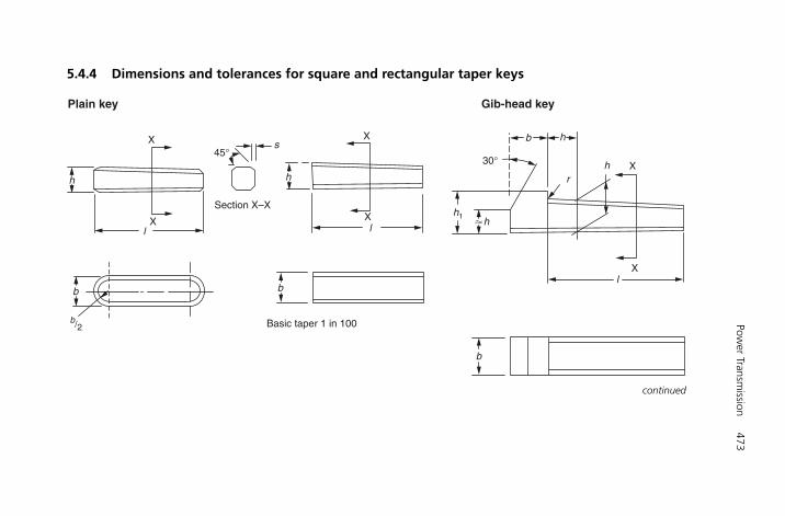
5.4.4 Dimensions and tolerances for square and rectangular taper keys
Power Transm
ission473
Section X–X
Plain key Gib-head key
Basic taper 1 in 100
X X
X
X
XX
45°
l l
l
b/2
b
h h
b
b
b
r
h
h
h�h1
s
30°
continued
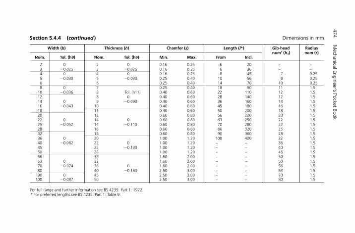
474M
echanical Engineer’s Pocket Book
Width (b) Thickness (h) Chamfer (s) Length (l*) Gib-head Radius nom� (h1) nom (r)
Nom. Tol. (h9) Nom. Tol. (h9) Min. Max. From Incl.
2 0 2 0 0.16 0.25 6 20 – –3 �0.025 3 �0.025 0.16 0.25 6 36 – –4 0 4 0 0.16 0.25 8 45 7 0.255 �0.030 5 �0.030 0.25 0.40 10 56 8 0.256 6 0.25 0.40 14 70 10 0.258 0 7 0.25 0.40 18 90 11 1.5
10 �0.036 8 Tol. (h11) 0.40 0.60 22 110 12 1.512 8 0 0.40 0.60 28 140 12 1.514 0 9 �0.090 0.40 0.60 36 160 14 1.516 �0.043 10 0.40 0.60 45 180 16 1.518 11 0.40 0.60 50 200 18 1.520 12 0.60 0.80 56 220 20 1.522 0 14 0 0.60 0.80 63 250 22 1.525 �0.052 14 �0.110 0.60 0.80 70 280 22 1.528 16 0.60 0.80 80 320 25 1.532 18 0.60 0.80 90 360 28 1.536 0 20 1.00 1.20 100 400 32 1.540 �0.062 22 0 1.00 1.20 – – 36 1.545 25 �0.130 1.00 1.20 – – 40 1.550 28 1.00 1.20 – – 45 1.556 32 1.60 2.00 – – 50 1.563 0 32 1.60 2.00 – – 50 1.570 �0.074 36 0 1.60 2.00 – – 56 1.580 40 �0.160 2.50 3.00 – – 63 1.590 0 45 2.50 3.00 – – 70 1.5
100 �0.087 50 2.50 3.00 – – 80 1.5
For full range and further information see BS 4235: Part 1: 1972.* For preferred lengths see BS 4235: Part 1: Table 9.
Section 5.4.4 (continued ) Dimensions in mm
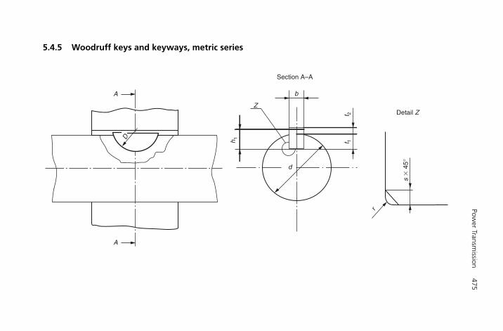
5.4.5 Woodruff keys and keyways, metric series
Power Transm
ission475
A
Z
b
r
D
t 2t 1h 1
Section A–A
Detail Z
A
s �
45°
d
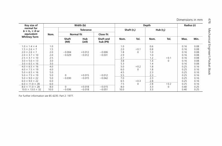
476M
echanical Engineer’s Pocket Book
Key size of Width (b) Depth Radius (r)normal for
Tolerance Shaft (t1) Hub (t2)b � h1 � D orNom. Normal fit Close fitequivalent
Shaft Hub Shaft and Nom. Tol. Nom. Tol. Max. Min.Whitney form
(N9) (Js9) hub (P9)
1.0 � 1.4 � 4 1.0 1.0 0.6 0.16 0.081.5 � 2.6 � 7 1.5 2.0 �0.1 0.8 0.16 0.082.0 � 2.6 � 7 2.0 �0.004 �0.012 �0.006 1.8 0 1.0 0.16 0.082.0 � 3.7 � 10 2.0 �0.029 �0.012 �0.031 2.9 1.0 0.16 0.082.5 � 3.7 � 10 2.5 2.7 1.2 �0.1 0.16 0.083.0 � 5.0 � 13 3.0 3.8 1.4 0 0.16 0.083.0 � 6.5 � 16 3.0 5.3 1.4 0.16 0.084.0 � 6.5 � 16 4.0 5.0 �0.2 1.8 0.25 0.164.0 � 7.5 � 19 4.0 6.0 0 1.8 0.25 0.165.0 � 6.5 � 16 5.0 4.5 2.3 0.25 0.165.0 � 7.5 � 19 5.0 0 �0.015 �0.012 5.5 2.3 0.25 0.165.0 � 9.0 � 22 5.0 �0.030 �0.015 �0.042 7.0 2.3 0.25 0.166.0 � 9.0 � 22 6.0 6.5 �0.3 2.8 0.25 0.166.0 � 11.0 � 28 6.0 7.5 0 2.8 �0.2 0.25 0.168.0 � 11.0 � 28 8.0 0 �0.018 �0.015 8.0 3.3 0 0.40 0.2510.0 � 13.0 � 32 10.0 �0.036 �0.018 �0.051 10.0 3.3 0.40 0.25
For further information see BS 4235: Part 2: 1977.
Dimensions in mm

5.4.6 Dimensions and tolerances for Woodruff Keys
Normal form
Whitney form
X X
s � 45°
s � 45°
X � Sharp edges removed
X � Sharp edges removed
X X
X X
b
dd
h 1h 2
b
Power Transmission 477
H6508-Ch05.4.qxd 9/12/05 4:50 PM Page 477
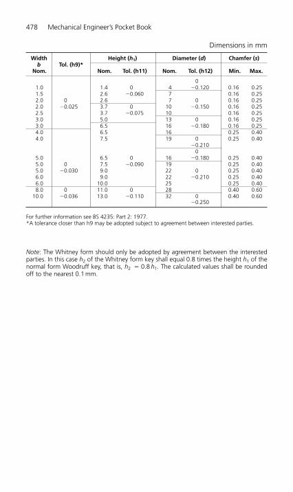
478 Mechanical Engineer’s Pocket Book
Width Height (h1) Diameter (d) Chamfer (s)b
Nom.Tol. (h9)*
Nom. Tol. (h11) Nom. Tol. (h12) Min. Max.
01.0 1.4 0 4 �0.120 0.16 0.251.5 2.6 �0.060 7 0.16 0.252.0 0 2.6 7 0 0.16 0.252.0 �0.025 3.7 0 10 �0.150 0.16 0.252.5 3.7 �0.075 10 0.16 0.253.0 5.0 13 0 0.16 0.253.0 6.5 16 �0.180 0.16 0.254.0 6.5 16 0.25 0.404.0 7.5 19 0 0.25 0.40
�0.2100
5.0 6.5 0 16 �0.180 0.25 0.405.0 0 7.5 �0.090 19 0.25 0.405.0 �0.030 9.0 22 0 0.25 0.406.0 9.0 22 �0.210 0.25 0.406.0 10.0 25 0.25 0.408.0 0 11.0 0 28 0.40 0.60
10.0 �0.036 13.0 �0.110 32 0 0.40 0.60�0.250
For further information see BS 4235: Part 2: 1977.*A tolerance closer than h9 may be adopted subject to agreement between interested parties.
Dimensions in mm
Note: The Whitney form should only be adopted by agreement between the interestedparties. In this case h2 of the Whitney form key shall equal 0.8 times the height h1 of thenormal form Woodruff key, that is, h2 � 0.8 h1. The calculated values shall be roundedoff to the nearest 0.1 mm.
H6508-Ch05.4.qxd 9/12/05 4:50 PM Page 478

5.4.7 Shaft ends types: general relationships
Cylindrical
Conical
Cylindrical
Short shaft ends
Conical
Long shaft ends
Power Transmission 479
H6508-Ch05.4.qxd 9/12/05 4:50 PM Page 479

5.4.8 Dimensions and tolerances of cylindrical shaft ends, long and short series
480M
echanical Engineer’s Pocket Book
X X
l1 l1
d1d1
Detail X: undercut grooves for tool relief and blendina radii are still under consideration in ISO. Details are not yet available.
Diameter (d1) Lengths (l1) Diameter (d1) Lengths (l1)
Nom. Tol. Long Short Nom. Tol. Long Shortseries series series series
j6�0.006
6 �0.002 100m6
�0.0357
16 –110 �0.013 210 165
8 j6�0.007 120
9 �0.002 20 –125
Dimensions in mm
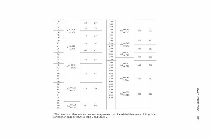
Power Transm
ission481
10 13011
23 20*140
1230 25*
15014
j6�0.008 160
m6�0.040
16 �0.003 170 �0.015250 200
18 40 28 18019 19020
50 36
200 300 24022 220
m6�0.046
24j6
�0.009 240 �0.01725 �0.004
60 42250 350 280
28 26030 280 m6
�0.052
32 300�0.020
410 33035 80 58 32038 34040
k6�0.018 360 m6
�0.057550 450
42 �0.002 380�0.021
45 40048 110 82 42050 44055 450 m6
�0.063650 540
56 460�0.023
60 48063
m6�0.030 500
65 �0.011140 105 530
70 560m6
�0.07071 600 �0.026
800 680
75 630808590 m6
�0.035 170 13095 �0.013
* The dimensions thus indicated are not in agreement with the related dimensions of long series conical shaft ends. See BS4506 Table 2 and Clause 2.
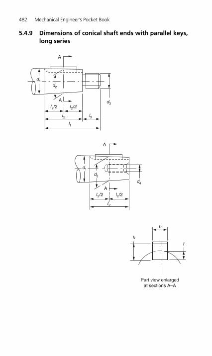
5.4.9 Dimensions of conical shaft ends with parallel keys,long series
A
A
A
A
b
ht
Part view enlargedat sections A–A
d3
d4
d2
d1
d2
d1
l3
l1
l2
l2
l2/2 l2/2
l2/2 l2/2
482 Mechanical Engineer’s Pocket Book
H6508-Ch05.4.qxd 9/12/05 4:50 PM Page 482
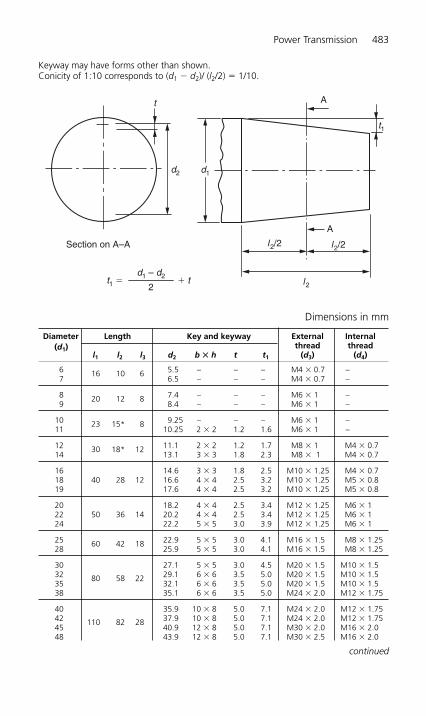
Power Transmission 483
Diameter Length Key and keyway External Internal thread thread (d1)
l1 l2 l3 d2 b � h t t1 (d3) (d4)
6 16 10 6 5.5 – – – M4 � 0.7 –7 6.5 – – – M4 � 0.7 –
8 20 12 8 7.4 – – – M6 � 1 –9 8.4 – – – M6 � 1 –
10 23 15* 8 9.25 – – – M6 � 1 –11 10.25 2 � 2 1.2 1.6 M6 � 1 –
12 30 18* 12 11.1 2 � 2 1.2 1.7 M8 � 1 M4 � 0.714 13.1 3 � 3 1.8 2.3 M8 � 1 M4 � 0.7
16 14.6 3 � 3 1.8 2.5 M10 � 1.25 M4 � 0.718 40 28 12 16.6 4 � 4 2.5 3.2 M10 � 1.25 M5 � 0.819 17.6 4 � 4 2.5 3.2 M10 � 1.25 M5 � 0.8
20 18.2 4 � 4 2.5 3.4 M12 � 1.25 M6 � 122 50 36 14 20.2 4 � 4 2.5 3.4 M12 � 1.25 M6 � 124 22.2 5 � 5 3.0 3.9 M12 � 1.25 M6 � 1
25 60 42 18 22.9 5 � 5 3.0 4.1 M16 � 1.5 M8 � 1.2528 25.9 5 � 5 3.0 4.1 M16 � 1.5 M8 � 1.25
30 27.1 5 � 5 3.0 4.5 M20 � 1.5 M10 � 1.532 80 58 22 29.1 6 � 6 3.5 5.0 M20 � 1.5 M10 � 1.535 32.1 6 � 6 3.5 5.0 M20 � 1.5 M10 � 1.538 35.1 6 � 6 3.5 5.0 M24 � 2.0 M12 � 1.75
40 35.9 10 � 8 5.0 7.1 M24 � 2.0 M12 � 1.7542 110 82 28 37.9 10 � 8 5.0 7.1 M24 � 2.0 M12 � 1.7545 40.9 12 � 8 5.0 7.1 M30 � 2.0 M16 � 2.048 43.9 12 � 8 5.0 7.1 M30 � 2.5 M16 � 2.0
continued
Dimensions in mm
Keyway may have forms other than shown. Conicity of 1:10 corresponds to (d1 � d2)/ (l2/2) � 1/10.
Section on A–A
t
d2 d1
t1
t1 � � td1 – d2
2
l2/2
A
A
l2/2
l2
H6508-Ch05.4.qxd 9/12/05 4:50 PM Page 483
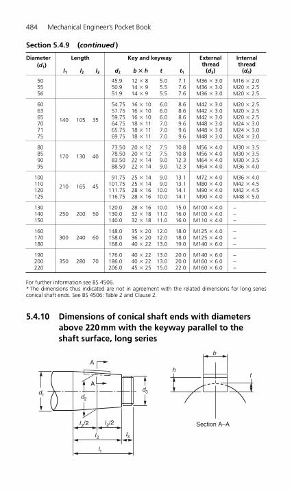
484 Mechanical Engineer’s Pocket Book
Diameter Length Key and keyway External Internal thread thread (d1)
l1 l2 l3 d2 b � h t t1 (d3) (d4)
50 45.9 12 � 8 5.0 7.1 M36 � 3.0 M16 � 2.055 50.9 14 � 9 5.5 7.6 M36 � 3.0 M20 � 2.556 51.9 14 � 9 5.5 7.6 M36 � 3.0 M20 � 2.5
60 54.75 16 � 10 6.0 8.6 M42 � 3.0 M20 � 2.563 57.75 16 � 10 6.0 8.6 M42 � 3.0 M20 � 2.565 140 105 35 59.75 16 � 10 6.0 8.6 M42 � 3.0 M20 � 2.570 64.75 18 � 11 7.0 9.6 M48 � 3.0 M24 � 3.071 65.75 18 � 11 7.0 9.6 M48 � 3.0 M24 � 3.075 69.75 18 � 11 7.0 9.6 M48 � 3.0 M24 � 3.0
80 73.50 20 � 12 7.5 10.8 M56 � 4.0 M30 � 3.585 170 130 40 78.50 20 � 12 7.5 10.8 M56 � 4.0 M30 � 3.590 83.50 22 � 14 9.0 12.3 M64 � 4.0 M30 � 3.595 88.50 22 � 14 9.0 12.3 M64 � 4.0 M36 � 4.0
100 91.75 25 � 14 9.0 13.1 M72 � 4.0 M36 � 4.0110 210 165 45 101.75 25 � 14 9.0 13.1 M80 � 4.0 M42 � 4.5120 111.75 28 � 16 10.0 14.1 M90 � 4.0 M42 � 4.5125 116.75 28 � 16 10.0 14.1 M90 � 4.0 M48 � 5.0
130 120.0 28 � 16 10.0 15.0 M100 � 4.0 –140 250 200 50 130.0 32 � 18 11.0 16.0 M100 � 4.0 –150 140.0 32 � 18 11.0 16.0 M110 � 4.0 –
160 148.0 35 � 20 12.0 18.0 M125 � 4.0 –170 300 240 60 158.0 36 � 20 12.0 18.0 M125 � 4.0 –180 168.0 40 � 22 13.0 19.0 M140 � 6.0 –
190 176.0 40 � 22 13.0 20.0 M140 � 6.0 –200 350 280 70 186.0 40 � 22 13.0 20.0 M160 � 6.0 –220 206.0 45 � 25 15.0 22.0 M160 � 6.0 –
For further information see BS 4506.* The dimensions thus indicated are not in agreement with the related dimensions for long seriesconical shaft ends. See BS 4506: Table 2 and Clause 2.
5.4.10 Dimensions of conical shaft ends with diametersabove 220 mm with the keyway parallel to the shaft surface, long series
A
Section A–A
d3
b
ht
d2d1
l3
l2/2 l2/2
l2
l1
A
Section 5.4.9 (continued )
H6508-Ch05.4.qxd 9/12/05 4:50 PM Page 484
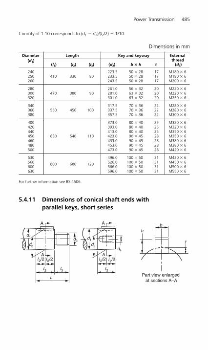
Power Transmission 485
Conicity of 1:10 corresponds to (d1 � d2)/(l2/2) � 1/10.
Dimensions in mm
Diameter Length Key and keyway Externalthread (d1)
(l1) (l2) (l3) (d2) b � h t (d3)
240 223.5 50 � 28 17 M180 � 6250 410 330 80 233.5 50 � 28 17 M180 � 6260 243.5 50 � 28 17 M200 � 6
280 261.0 56 � 32 20 M220 � 6300 470 380 90 281.0 63 � 32 20 M220 � 6320 301.0 63 � 32 20 M250 � 6
340 317.5 70 � 36 22 M280 � 6360 550 450 100 337.5 70 � 36 22 M280 � 6380 357.5 70 � 36 22 M300 � 6
400 373.0 80 � 40 25 M320 � 6420 393.0 80 � 40 25 M320 � 6440 413.0 80 � 40 25 M350 � 6450 650 540 110 423.0 90 � 45 28 M350 � 6460 433.0 90 � 45 28 M380 � 6480 453.0 90 � 45 28 M380 � 6500 473.0 90 � 45 28 M420 � 6
530 496.0 100 � 50 31 M420 � 6560 800 680 120 526.0 100 � 50 31 M450 � 6600 566.0 100 � 50 31 M500 � 6630 596.0 100 � 50 31 M550 � 6
For further information see BS 4506.
5.4.11 Dimensions of conical shaft ends with parallel keys, short series
A A
AA
l2 l2
l1
l3
d2
d1 d3d1
d2d4
l2/2 l2/2 l2/2 l2/2
Part view enlarged at sections A–A
bh
t
H6508-Ch05.4.qxd 9/12/05 4:50 PM Page 485

Keyway may have forms other than shown.Conicity of 1:10 corresponds to (d1 � d2)/(l2/2) � 1/10.
t
d2 d1
t1
t1 � � td1 – d2
2
l2/2
A
A
l2/2
l2
486 Mechanical Engineer’s Pocket Book
Diameter Length Key and key way External Internal thread thread (d1)
(l1) (l2) (l3) (l2) b � h t t1 (d3) (d4)
16 15.2 3 � 3 1.8 M10 � 1.25 M4 � 0.718 28 16 12 17.2 4 � 4 2.5 M10 � 1.25 M5 � 0.819 18.2 4 � 4 2.5 M10 � 1.25 M5 � 0.8
20 18.9 4 � 4 2.5 M12 � 1.25 M6 � 1.022 36 22 14 20.9 4 � 4 2.5 M12 � 1.25 M6 � 1.024 22.9 5 � 5 3.0 M12 � 1.25 M6 � 1.0
25 42 24 18 23.8 5 � 5 3.0 M16 � 1.5 M8 � 1.2528 26.8 5 � 5 3.0 M16 � 1.5 M8 � 1.25
30 28.2 5 � 5 3.0 M20 � 1.5 M10 � 1.532 58 36 22 30.2 6 � 6 3.5 M20 � 1.5 M10 � 1.535 33.2 6 � 6 3.5 M20 � 1.5 M10 � 1.538 36.2 6 � 6 3.5 M24 � 2.0 M12 � 1.75
40 37.3 10 � 8 5.0 M24 � 2 M12 � 1.7542 39.3 10 � 8 5.0 M24 � 2 M12 � 1.7545 42.3 12 � 8 5.0 M30 � 2 M16 � 2.048 82 54 28 45.3 12 � 8 5.0 M30 � 2 M16 � 2.050 47.3 12 � 8 5.0 M36 � 3 M16 � 2.055 52.3 14 � 9 5.5 M36 � 3 M20 � 2.556 53.3 14 � 9 5.5 M36 � 3 M20 � 2.5
60 56.5 16 � 10 6.0 M42 � 3 M20 � 2.563 59.5 16 � 10 6.0 M42 � 3 M20 � 2.565 105 70 35 61.5 16 � 10 6.0 M42 � 3 M20 � 2.570 66.5 18 � 11 7.0 M48 � 3 M24 � 3.071 67.5 18 � 11 7.0 M48 � 3 M24 � 3.075 71.5 18 � 11 7.0 M48 � 3 M24 � 3.0
Dimensions in mm
continued
H6508-Ch05.4.qxd 9/12/05 4:50 PM Page 486
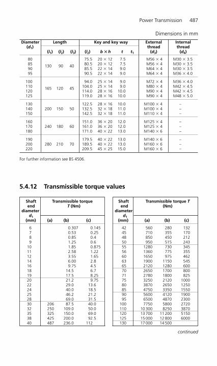
Power Transmission 487
Diameter Length Key and key way External Internal thread thread (d1)
(l1) (l2) (l3) (l2) b � h t t1 (d3) (d4)
80 75.5 20 � 12 7.5 M56 � 4 M30 � 3.585 130 90 40 80.5 20 � 12 7.5 M56 � 4 M30 � 3.590 85.5 22 � 14 9.0 M64 � 4 M30 � 3.595 90.5 22 � 14 9.0 M64 � 4 M36 � 4.0
100 94.0 25 � 14 9.0 M72 � 4 M36 � 4.0110 165 120 45 104.0 25 � 14 9.0 M80 � 4 M42 � 4.5120 114.0 28 � 16 10.0 M90 � 4 M42 � 4.5125 119.0 28 � 16 10.0 M90 � 4 M48 � 5.0
130 122.5 28 � 16 10.0 M100 � 4 –140 200 150 50 132.5 32 � 18 11.0 M100 � 4 –150 142.5 32 � 18 11.0 M110 � 4 –
160 151.0 36 � 20 12.0 M125 � 4 –170 240 180 60 161.0 36 � 20 12.0 M125 � 4 –180 171.0 40 � 22 13.0 M140 � 6 –
190 179.5 40 � 22 13.0 M140 � 6 –200 280 210 70 189.5 40 � 22 13.0 M160 � 6 –220 209.5 45 � 25 15.0 M160 � 6 –
For further information see BS 4506.
Dimensions in mm
continued
Shaft Transmissible torque end T (Nm)
diameterd1
(mm) (a) (b) (c)
6 0.307 0.1457 0.53 0.258 0.85 0.49 1.25 0.6
10 1.85 0.87511 2.58 1.2212 3.55 1.6514 6.00 2.816 9.75 4.518 14.5 6.719 17.5 8.2520 21.2 9.7522 29.0 13.624 40.0 18.525 46.2 21.228 69.0 31.530 206 87.5 40.032 250 109.0 50.035 325 150.0 69.038 425 200.0 92.540 487 236.0 112
Shaft Transmissible torque Tend (Nm)
diameterd1
(mm) (a) (b) (c)
42 560 280 13245 710 355 17048 850 450 21250 950 515 24355 1280 730 34556 1360 775 35560 1650 975 46263 1900 1150 54565 2120 1280 60070 2650 1700 80071 2780 1800 82575 3250 2120 100080 3870 2650 125085 4750 3350 155090 5600 4120 190095 6500 4870 2300
100 7750 5800 2720110 10 300 8250 3870120 13 700 11 200 5150125 15 000 12 800 6000130 17 000 14 500
5.4.12 Transmissible torque values
H6508-Ch05.4.qxd 9/12/05 4:50 PM Page 487
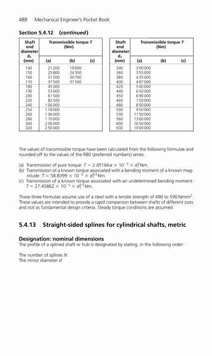
488 Mechanical Engineer’s Pocket Book
The values of transmissible torque have been calculated from the following formulae androunded off to the values of the R80 (preferred numbers) series:
(a) Transmission of pure torque: T � 2.45166� � 10�3 � d13Nm.
(b) Transmission of a known torque associated with a bending moment of a known mag-nitude: T � 58.8399 � 10�5 � d1
3.5Nm.(c) Transmission of a known torque associated with an undetermined bending moment:
T � 27.45862 � 10�5 � d13.5Nm.
These three formulae assume use of a steel with a tensile strength of 490 to 590 N/mm2.These values are intended to provide a rapid comparison between shafts of different sizesand not as fundamental design criteria. Steady torque conditions are assumed.
5.4.13 Straight-sided splines for cylindrical shafts, metric
Designation: nominal dimensionsThe profile of a splined shaft or hub is designated by stating, in the following order:
The number of splines NThe minor diameter d
Shaft Transmissible torque Tend (Nm)
diameterd1
(mm) (a) (b) (c)
140 21 200 19 000150 25 800 24 300160 31 500 30 700170 37 500 37 500180 45 000190 53 000200 61 500220 82 500240 1 06 000250 1 18 000260 1 36 000280 1 70 000300 2 06 000320 2 50 000
Shaft Transmissible torque Tend (Nm)
diameterd1
(mm) (a) (b) (c)
340 3 00 000360 3 55 000380 4 25 000400 4 87 000420 5 60 000440 6 50 000450 6 90 000460 7 50 000480 8 50 000500 9 50 000530 11 50 000560 13 60 000600 16 50 000630 19 00 000
Section 5.4.12 (continued )
H6508-Ch05.4.qxd 9/12/05 4:50 PM Page 488

Power Transmission 489
The outside diameter D.For example, shaft (or hub) 6 � 23 � 26.
D
d B
d Light series Medium series(mm)
Designation N D B Designation N D B(mm) (mm) (mm) (mm)
11 6 � 11 � 14 6 14 313 6 � 13 � 16 6 16 3.516 6 � 16 � 20 6 20 418 6 � 18 � 22 6 22 5
21 6 � 21 � 25 6 25 523 6 � 23 � 26 6 26 6 6 � 23 � 28 6 28 626 6 � 26 � 30 6 30 6 6 � 26 � 32 6 32 628 6 � 28 � 32 6 32 7 6 � 28 � 34 6 34 7
32 8 � 32 � 36 8 36 6 8 � 32 � 38 8 38 636 8 � 36 � 40 8 40 7 8 � 36 � 42 8 42 742 8 � 42 � 46 8 46 8 8 � 42 � 48 8 48 846 8 � 46 � 50 8 50 9 8 � 46 � 54 8 54 9
52 8 � 52 � 58 8 58 10 8 � 52 � 60 8 60 1056 8 � 56 � 62 8 62 10 8 � 56 � 65 8 65 1062 8 � 62 � 68 8 68 12 8 � 62 � 72 8 72 12
72 10 � 72 � 78 10 78 12 10 � 72 � 82 10 82 1282 10 � 82 � 88 10 88 12 10 � 82 � 92 10 92 1292 10 � 92 � 98 10 98 14 10 � 92 � 102 10 102 14
102 10 � 102 � 108 10 108 16 10 � 102 � 112 10 112 16112 10 � 112 � 120 10 120 18 10 � 112 � 125 10 125 18
Section 5.4.13 (continued )
H6508-Ch05.4.qxd 9/12/05 4:50 PM Page 489
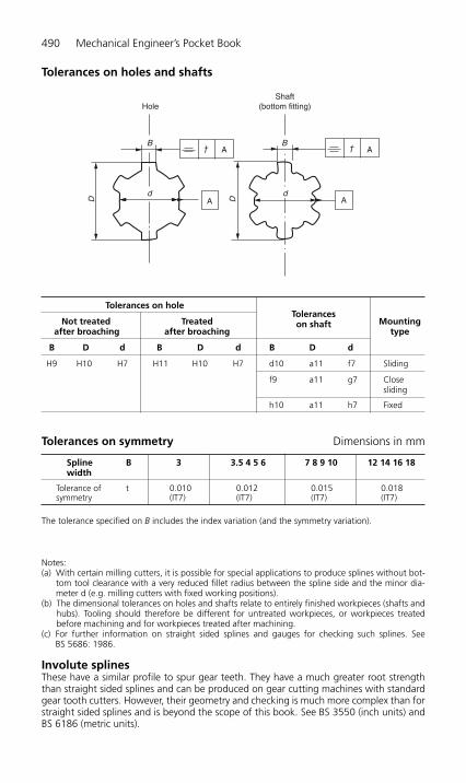
Tolerances on holes and shafts
B B
dA
Shaft(bottom fitting)Hole
A
AD D
†A†
d
490 Mechanical Engineer’s Pocket Book
Tolerances on hole
Not treated Treated Tolerances
Mountingafter broaching after broaching
on shafttype
B D d B D d B D d
H9 H10 H7 H11 H10 H7 d10 a11 f7 Sliding
f9 a11 g7 Close sliding
h10 a11 h7 Fixed
Tolerances on symmetry Dimensions in mm
Spline B 3 3.5 4 5 6 7 8 9 10 12 14 16 18width
Tolerance of t 0.010 0.012 0.015 0.018 symmetry (IT7) (IT7) (IT7) (IT7)
The tolerance specified on B includes the index variation (and the symmetry variation).
Notes:(a) With certain milling cutters, it is possible for special applications to produce splines without bot-
tom tool clearance with a very reduced fillet radius between the spline side and the minor dia-meter d (e.g. milling cutters with fixed working positions).
(b) The dimensional tolerances on holes and shafts relate to entirely finished workpieces (shafts andhubs). Tooling should therefore be different for untreated workpieces, or workpieces treatedbefore machining and for workpieces treated after machining.
(c) For further information on straight sided splines and gauges for checking such splines. See BS 5686: 1986.
Involute splinesThese have a similar profile to spur gear teeth. They have a much greater root strengththan straight sided splines and can be produced on gear cutting machines with standardgear tooth cutters. However, their geometry and checking is much more complex than forstraight sided splines and is beyond the scope of this book. See BS 3550 (inch units) andBS 6186 (metric units).
H6508-Ch05.4.qxd 9/12/05 4:50 PM Page 490
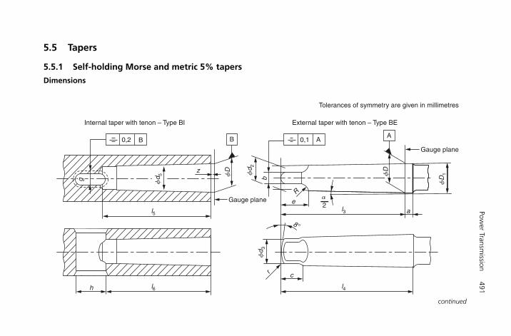
Power Transm
ission491
5.5 Tapers
5.5.1 Self-holding Morse and metric 5% tapers
Dimensions
fD
1fd 2
fd 3
fD
fd 5 f
D
0,2 B
Internal taper with tenon – Type BI External taper with tenon – Type BE
Tolerances of symmetry are given in millimetres
0,1
2
AB
Gauge plane
Gauge plane
z
l6h
l5 l3
l4
b
e
cr
aR
A
a
8°
g
continued
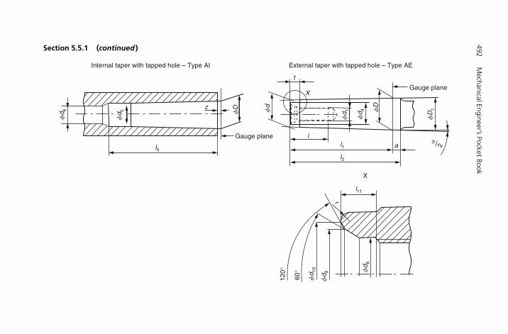
492M
echanical Engineer’s Pocket Book
fD fd
fd 1
fd 1
0 fd 8
fd 9
fd 4 f
D
fD
1z
i
X
X
a
r
l1
l2
l11
t
l5
fd 5
fd 6
Gauge plane
Internal taper with tapped hole – Type AI External taper with tapped hole – Type AE
Gauge plane
�2
60°
120°
Section 5.5.1 (continued )
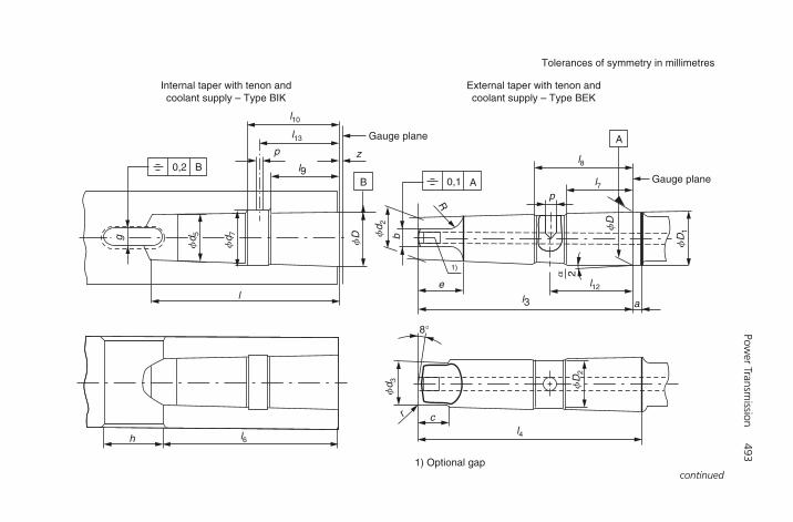
Power Transm
ission493
Tolerances of symmetry in millimetres
External taper with tenon andcoolant supply – Type BEK
Internal taper with tenon andcoolant supply – Type BIK
Gauge plane
Gauge plane
l10
l13
l9
l3
l12
al
l6l4
l8
l7
z
g
B
A
B
b
p
p
h
a 2
e
cr
1)
1) Optional gap
8°
0,2
A
R
0,1
fd 2
fd 3
fD
fD
fD
1
fd 5
fd 7
fD
2
continued
494M
echanical Engineer’s Pocket Book
Internal taper with tapped holeand coolant supply – Type AIK Gauge plane
Gauge plane
External taper with tapped holeand coolant supply – Type AEK
z
t
i
X
X
a — 2
fd 6
fd 5
fd 7
fd 4
l8
a
r
l1l2
l11
l12
l7
fd 1
fd 8fd 1
0
fd 9
fD
1fD
fd
fD
p
l10
l13
l9
l5
120°
60°
p
fD
2
Section 5.5.1 (continued )
Metric Designation tapers Morse tapers Metric tapers
4 6 0 1 2 3 4 5 6 80 100 120 160 200
Taper ratio 1:20 0.624 6:12 0.598 58:12 0.599 41:12 0.602 35:12 0.623 26:12 0.631 51:12 0,62565:12 1:20 � 0,05� 0,05 � 1:19.212 � 1:20.047 � 1:20.02 � 1:19.922 � 1:19.254 � 1:19.002 � 1:19.18
� 0.052 05 � 0.049 88 � 0.049 95 � 0.050 2 � 0.051 94 � 0.052 63 � 0.052 14
External D 4 6 9.045 12.065 17.78 23.825 31.267 44.399 63.348 80 100 120 160 200taper a 2 3 3 3.5 5 5 6.5 6.5 8 8 10 12 16 20
D1 (1) 4.1 6.2 9.2 12.2 18 24.1 31.6 44.7 63.8 80.4 100.5 120.6 160.8 201D2 – – – – 15 21 26 40 56 – – – – –d (1) 2.9 4.4 6.4 9.4 14.6 19.8 25.9 37.6 53.9 70.2 88.4 106.6 143 179.4d1 (2) – – – M6 M10 M12 M16 M20 M24 M30 M36 M36 M48 M48d2 (1) – – 6.1 9 14 19.1 25.2 36.5 52.4 69 87 105 141 177d3 max. – – 6 8.7 13.5 18.5 24.5 35.7 51 67 85 102 138 174d4 max. 2.5 4 6 9 14 19 25 35.7 51 67 85 102 138 174d8 – – – 6.4 10.5 13 17 21 26 – – – – –d9 – – – 8 12.5 15 20 26 31 – – – – –d10 max. – – – 8.5 13.2 17 22 30 11.5 – – – – –l1 max. 23 32 50 53.5 64 81 102.5 129.5 182 196 232 268 340 412l2 max. 25 35 53 57 69 86 109 136 190 204 242 280 356 432l3 0
�0.1 – – 56.5 62 75 94 117.5 149.5 210 220 260 300 380 460l4 max. – – 59.5 65.5 80 99 124 156 218 228 270 312 396 480l7 0
�0.1 – – – – 20 29 39 51 81 – – – – –l8 0
0.1 – – – – 34 43 55 69 99 – – – – –l11 – – – 4 5 5.5 8.2 10 11.5 – – – – –l12 – – – – 27 36 47 60 90 – – – – –p – – – 3.3 4.2 5 6.8 8.5 10.2 – – – – –b h13 – – 3.9 5.2 6.3 7.9 11.9 15.9 19 26 32 38 50 62c (3) – – 6.5 8.5 10 13 16 19 27 24 28 32 40 48e max. – – 10.5 13.5 16 20 24 29 40 48 58 68 88 108
continued
Numbers 0–6 Morse tapers and 5% metric tapers Dimensions in mm
DesignationMetric tapers Morse tapers Metric tapers
4 6 0 1 2 3 4 5 6 80 100 120 160 200
Taper ratio 1:20 0.624 6:12 0.598 58:12 0.599 41:12 0.602 35:12 0.623 26:12 0.631 51:12 0.62565:12 1:20 � 0,05� 0.05 � 1:19,212 � 1:20.047 � 1:20,02 � 1:19.922 � 1:19.254 � 1:19.002 � 1:19.18
� 0,052 05 � 0.049 88 � 0.049 95 � 0.050 2 � 0.051 94 � 0.052 63 � 0.052 14
i min. – – – 16 24 24 32 40 47 59 70 70 92 92R max. – – 4 5 6 7 8 12 18 24 30 36 48 60r – – 1 1.2 1.6 2 2.5 3 4 5 5 6 8 10t max. 2 3 4 5 5 7 9 10 16 24 30 36 48 60
Internal d5 H11 3 4.6 6.7 9.7 14.9 20.2 26.5 38.2 54.8 71.5 90 108.5 145.5 182.5taper d6 min. – – – 7 11.5 14 18 23 27 33 39 39 52 52
d7 – – – – 19.5 24.5 32 44 63 – – – – –l5 min. 25 34 52 56 67 84 107 135 188 202 240 276 350 424l6 21 29 49 52 62 78 98 125 177 186 220 254 321 388l9 – – – – 22 31 41 53 83 – – – – –l10 – – – – 32 41 53 67 97 – – – – –l13 – – – – 27 36 47 60 90 – – – – –g A13 2.2 3.2 3.9 5.2 6.3 7.9 11.9 15.9 19 26 32 38 50 62h 8 12 15 19 22 27 32 38 47 52 60 70 90 110p – – – – 4.2 5 6.8 8.5 10.2 – – – – –z (4) 0.5 0.5 1 1 1 1 1 1 1 1.5 1.5 1.5 2 2
(1) For D1 and d or d2, approximate values are given for guidance. (The actual values result from the actual values of a and l1 or l3 respectively, taking into account the taper ratio and the basic size D.)
(2) d1 is the nominal thread diameter, either a metric thread M with standard pitch or, if expressly stated, a UNC thread (see table ‘Numbers 1–6 Morse tapers and Numbers1–3 (Brown & Sharpe tapers’ for inch sizes). In every case, the appropriate symbol M or UNC shall be marked on the component.
(3) It is permissible to increase the length c over which the tenon is turned to diameter d3, but without exceeding e.(4) z is the maximum permissible deviation, outwards only, of the position of the gauge plane related to the basic size D from the nominal position of coincidence with the
leading face.
Section 5.5.1 (continued) Dimensions in mm

DesignationBrown & Sharpe tapers Morse tapers
1 2 3 1 2 3 4 5 6
Taper ratio 0.502:12 0.502:12 0.502:12 0.598 58:12 0.599 41:12 0.602 35:12 0.623 26:12 0.631 51:12 0.625 65:12� 1:23,904 � 1:23,904 � 1:23,904 � 1:20,047 � 1:20,02 � 1:19,922 � 1:19,254 � 1:19,002 � 1:19,18� 0.041 83 � 0.041 83 � 0.041 83 � 0.049 88 � 0.049 95 � 0.050 2 � 0.051 94 � 0.052 63 � 0.052 14
External D 0.239 22 0.299 68 0.375 25 0.475 0.7 0.938 1.231 1.748 2.494taper a 3/32 3/32 3/32 1/8 3/16 3/16 1/4 1/4 1/16
D1 (1) 0.243 14 0.303 6 0.379 17 0.481 2 0.709 4 0.947 4 1.244 1.761 2 2.510 3D2 – – – 0.393 7 0.590 6 0.826 8 1.102 4 1.574 8 2.204 7d (1) 0.2 0.25 0.312 5 0.369 0.572 0.778 1.02 1.475 2.116d1 (2) – – – UNC 1/4 UNC 3/8 UNC 1/2 UNC 5/8 UNC 5/8 UNC 1d2 (1) 0.189 54 0.236 93 0.296 81 0.353 4 0.553 3 0.752 9 0.990 8 1.438 8 2.063 9d3 max. 11/64 7/32 9/32 11/32 17/32 23/32 31/32 1 13/32 2d4 max. 11/64 7/32 9/32 11/32 17/32 23/32 31/32 1 13/32 2d8 – – – 0.251 97 0.413 38 0.511 81 0.669 29 0.826 77 1.023 62d9 – – – 0.314 96 0.492 12 0.590 55 0.787 4 1.023 62 1.220 47d10 max. – – – 0.334 64 0.519 68 0.689 29 0.866 14 1.181 1 1.417 32l1 max. 15/16 1 3/16 1 1/2 2 1/8 2 9/16 3 3/16 4 1/16 5 3/16 7 1/4l2 max. 1 1/32 1 9/32 1 19/32 2 1/4 2 3/4 3 3/8 4 5/16 5 7/16 7 9/16l3 0
�0.004 1 3/16 1 1/2 1 7/8 2 7/16 2 15/16 3 11/16 4 5/8 5 7/8 8 1/4l4 max. 1 9/32 1 19/32 1 31/32 2 9/16 3 1/8 3 7/8 4 7/8 6 1/8 8 9/16l7 0
�0.004 – – – 19/32 25/32 1 9/64 1 17/32 2 3 3/16l8 0
�0.004 – – – 1 3/16 1 11/32 1 19/64 2 3/16 2 23/32 3 29/32l11 – – – 0.157 48 0.196 85 0.216 53 0.322 83 0.393 7 0.452 75l12 – – – – 1.062 99 1.417 32 1.850 39 2.362 2 3.543 3p – – – 1/8 11/64 13/64 9/32 21/64 13/32b h12 0.125 0.156 2 0.187 5 0.203 1 0.25 0.312 5 0.468 7 0.625 0.75
continued
Numbers 1–6 Morse tapers and Nos 1–3 Brown & Sharpe tapers Dimensions in mm
DesignationBrown & Sharpe tapers Morse tapers
1 2 3 1 2 3 4 5 6
Taper ratio 0.502:12 0.502:12 0.502:12 0.598 58:12 0.599 41:12 0.602 35:12 0.623 26:12 0.631 51:12 0.625 65:12� 1:23,904 � 1:23,904 � 1:23,904 � 1:20,047 � 1:20,02 � 1:19,922 � 1:19,254 � 1:19,002 � 1:19,18� 0.041 83 � 0.041 83 � 0.041 83 � 0.049 88 � 0.049 95 � 0.050 2 � 0,051 94 � 0.052 63 � 0.052 14
c (3) 1/4 5/16 3/8 11/32 13/32 17/32 5/8 3/4 1 1/16e max. 0.381 0.455 0.532 0.52 0.66 0.83 0.96 1.15 1.58i min. – – – 1/2 3/4 0.944 88 1 1/4 1 1/4 1.850 4R max. 3/16 3/16 3/16 3/16 1/4 9/32 5/16 0.472 44 0.708 66r 1/32 1/32 3/64 3/64 1/16 5/64 3/32 1/8 5/32t max. 1/8 1/8 1/8 3/16 3/16 1/4 1/4 5/16 3/8
Internal d5 H11 0.203 0.255 0.319 0.378 0.588 0.797 1.044 1.502 2.157 48taper d6 min. – – – 9/32 7/16 9/16 11/16 11/16 1 1/8
d7 – – – 17/32 49/64 31/32 1 17/64 1 47/64 2 31/64l5 min. 1 1 1/4 1 9/16 2 3/16 2 21/32 3 9/32 4 5/32 5 5/16 7 3/8l6 29/32 1 1/8 1 13/32 2 1/16 2 1/2 3 1/16 3 7/8 4 15/16 7l9 – – – 43/64 7/8 17/32 1 39/64 2 3/32 3 17/64l10 – – – 1 1/16 1 17/64 1 39/64 2 3/32 2 41/64 3 13/16l13 – – – – 1.062 99 1.417 32 1.850 39 2.362 2 3.543 3g H12 0.141 0.172 0.203 0.223 0.27 0.333 0.493 0.65 0.78h 13/32 9/16 23/32 3/4 7/8 1 1/8 1 1/4 1 1/2 1 7/8p – – – 1/8 11/64 13/64 9/32 21/64 13/32z (4) 0.04 0.04 0.04 0.039 3 0.039 3 0.039 3 0.039 3 0.039 3 0.039 3
Section 5.5.1 (continued) Dimensions in mm
(1) For D1 and d or d2, approximate values are given for guidance.(The actual values result from the actual values of a and l1 or l3 respectively, taking into account the taper ratio and the basic size D.)
(2) d1 is the nominal thread diameter: either a UNC thread or, if expressly stated, a metric thread M with standard pitch (see table ‘Numbers 1–6 Morse tapers and 5% metrictapers’ for metric sizes). In every case, the appropriate symbol UNC or M shall be marked on the component.
(3) It is permissible to increase the length c over which the tenon is turned to diameter d3, but without exceeding e.(4) z is the maximum permissible deviation, outwards only, of the position of the gauge plane related to the basic size D from the nominal position of coincidence with the
leading face.
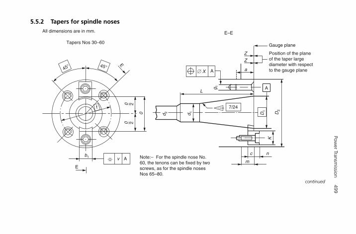
Power Transm
ission499
All dimensions are in mm.
Tapers Nos 30–60
E
f
45° 45°
0
0 – 20 – 2
b1
E
A Note:– For the spindle nose No.60, the tenons can be fixed by twoscrews, as for the spindle nosesNos 65–80.
v–—–
Z
Z
a
Gauge plane
Position of the planeof the taper largediameter with respectto the gauge plane
A
7/24
D1
D2
d 1
g 1
L
d 2
K
nc
m
� X A
E–E
5.5.2 Tapers for spindle noses
continued
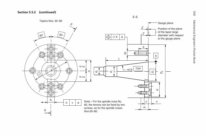
500M
echanical Engineer’s Pocket Book
Tapers Nos. 65–80
30° 30°
f
E
v A
A
A
E
0 – 2
0
0 – 2
–—–b1
d 1 D1
D2
Z
Z
c n
m
K
d 2
Note:– For the spindle nose No.60, the tenons can be fixed by twoscrews, as for the spindle nosesNos 65–80.
7/24
L
Gauge plane
Position of the planeof the taper largediameter with respectto the gauge plane� X
E–E
a
g 1
Section 5.5.2 (continued )

Power Transm
ission501
DesignationTaper Recess (2) Tenon External centring
No. D1 (1) z d1 L d2 b1 v c n O/2 K D2 m f g1 a xH12 min. min. (3) min. max. min. max. h5 min. (4) min.
30 31.75 0.4 17.4 73 17 15.9 0.06 8 8 16.5 16.5 69.832 12.5 54 M10 16 0.1540 44.45 0.4 25.3 100 17 15.9 0.06 8 8 23 19.5 88.882 16 66.7 M12 20 0.1545 57.15 0.4 32.4 120 21 19 0.06 9.5 9.5 30 19.5 101.6 18 80 M12 20 0.1550 69.85 0.4 39.6 140 27 25.4 0.08 12.5 12.5 36 26.5 128.57 19 101.6 M16 25 0.255 88.9 0.4 50.4 178 27 25.4 0.08 12.5 12.5 48 26.5 152.4 25 120.6 M20 30 0.260 107.95 0.4 60.2 220 35 25.4 0.08 12.5 12.5 61 45.5 221.44 38 177.8 M20 30 0.265 133.35 0.4 75 265 42 32 0.1 16 16 75 58 280 38 220 M24 36 0.2570 165.1 0.4 92 315 42 32 0.1 20 20 90 68 335 50 265 M24 45 0.2575 203.2 0.4 114 400 56 40 0.1 25 25 108 86 400 50 315 M30 56 0.3280 254 0.4 140 500 56 40 0.1 31.5 31.5 136 106 500 50 400 M30 63 0.32
(1) D1: Basic diameter defining the gauge plane.(2) Opening for traction bar.(3) Assembly of the tenon in the slot: M6-h5 fit.(4) Thread diameter g1: this is either a metric thread M with coarse pitch or, if expressly stated, a UN thread according to table ‘on thread specification’. In every case,
the appropriate symbol M or UN shall be marked on the component.
Designation and dimensions

502M
echanical Engineer’s Pocket Book
Designation 30 40 45 50 55 60 65 70 75 80No.
g1 UN UN UN UN UN UN UN UN UN UN 0,375-16 0,500-13 0,500-13 0,625-11 0,750-10 0,750-10 1,000-8 1,000-8 1,250-7 1,250-7
Thread specification
Installation of tenons
Noses Nos 65–80
Tenons
� �
��
b1
l6
ug 2 d 5
d 4
s � 45°
30°
K
h
e
q
Note:– For spindle nose No. 60, the tenons can be fixed by two screws, as for the spindle noses Nos 65–80.
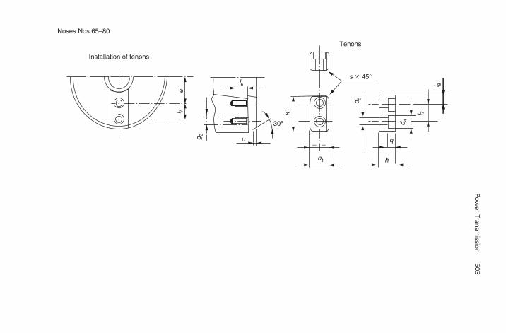
Power Transm
ission503
Installation of tenons
Noses Nos 65–80
Tenons
b1
l6
g 2
l 7
d 5
d 4
l 7
l 8
s � 45°
30º
K
h
e
u q� �

504M
echanical Engineer’s Pocket Book
Designation Tenon Slot Chamfer
No. b1 h k d5 d4 q l7 l8 s e � 0.2 g2 l6 l7 Screws ISO 4762 umax. max. max.
30 16 16.5 6.4 10.4 7 – – 1.6 25 M6 9 – M6 � 16 240 16 19.5 6.4 10.4 7 – – 1.6 33 M6 9 – M6 � 16 245 19 19.5 8.4 13.4 9 – – 1.6 40 M8 12 – M8 � 20 250 25 26.5 13 19 13 – – 2 49.5 M12 18 – M12 � 25 355 25 26.5 13 19 13 – – 2 61.5 M12 18 – M12 � 25 360 25 45.5 13 19 13 – – 2 84 M12 18 – M12 � 25 3
25 45.5 13 19 13 22 11.7 2 73 M12 18 22 M12 � 25 365 32 58 17 25 17 28 15 2.5 90 M16 25 28 M16 � 35 470 40 68 17 25 17 36 16 2.5 106 M16 25 36 M16 � 45 475 50 86 21 31 21 42 22 2.5 130 M20 30 42 M20 � 55 480 63 106 21 31 21 58 24 2.5 160 M20 30 58 M20 � 65 4
See
Tabl
e 1(
a)
Complementary dimensions
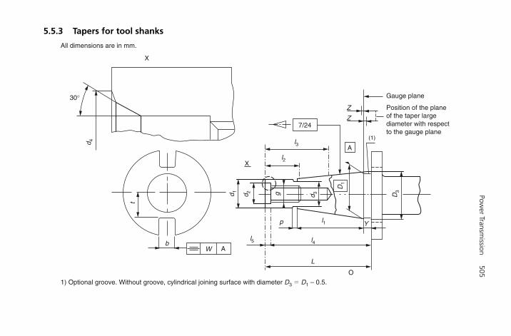
Power Transm
ission505
All dimensions are in mm.
Gauge plane
Position of the planeof the taper largediameter with respectto the gauge plane
X
X
7/24
30°
Y
A
(1)
d 4
d 2
D1
D3
d 1
l2
l3
l5 l4
l1p
L
O
W Ab
t
g d 3
1) Optional groove. Without groove, cylindrical joining surface with diameter D3 � D1 – 0.5.
Z
Z
5.5.3 Tapers for tool shanks
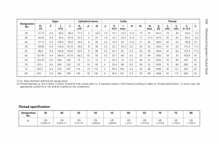
506M
echanical Engineer’s Pocket Book
DesignationTaper Cylindrical tenon Collar Thread
No. D1 Z L l1 d1 p d3 y b t w d2 d4 g l2 l3 l4 l5(1) h12 a10 H12 max. max. (2) min. min. 0�0.5
30 31.75 0.4 68.4 48.4 17.4 3 16.5 1.6 16.1 16.2 0.12 13 16 M12 24 34 62.9 5.5
40 44.45 0.4 93.4 65.4 25.3 5 24 1.6 16.1 22.5 0.12 17 21.5 M16 32 43 85.2 8.2
45 57.15 0.4 106.8 82.8 32.4 6 30 3.2 19.3 29 0.12 21 26 M20 40 53 96.8 10
50 69.85 0.4 126.8 101.8 39.6 8 38 3.2 25.7 35.3 0.2 26 32 M24 47 62 115.3 11.5
55 88.9 0.4 164.8 126.8 50.4 9 48 3.2 25.7 45 0.2 26 36 M24 47 62 153.3 11.5
60 107.95 0.4 206.8 161.8 60.2 10 58 3.2 25.7 60 0.2 32 44 M30 59 76 192.8 14
65 133.35 0.4 246 202 75 12 72 4 32.4 72 0.3 38 52 M36 70 89 230 16
70 165.1 0.4 296 252 92 14 90 4 32.4 86 0.3 38 52 M36 70 89 280 16
75 203.2 0.4 370 307 114 16 110 5 40.5 104 0.3 50 68 M48 92 115 350 20
80 254 0.4 469 394 140 18 136 6 40.5 132 0.3 50 68 M48 92 115 449 20
Designation 30 40 45 50 55 60 65 70 75 80No.
g UN UN UN UN UN UN UN UN UN UN 0,500-13 0,625-11 0,75-10 1,000-8 1,000-8 1,25-7 1,375-6 1,375-6 1,750-5 1,750-5
Thread specification
(1) D1: Basic diameter defining the gauge plane.(2) Thread diameter g: this is either a metric thread M with coarse pitch or, if expressly stated, a UN thread according to table on ‘thread specification’. In every case, the
appropriate symbol M or UN shall be marked on the component.

Power Transmission 507
5.5.4 Tool shank collars
Designation and dimensions
Gauge plane
All dimensions are in mm.
End of taper
7/24D
1
D4
D
i
j
Designation D1 ia,b D D4b jb,c
No. � 0,1 max. min.
30 31.75 9.6 50 36 9
40 44.45 11.6 63 50 11
45 57.1515.2
80 68 13
50 69.85 97.5 78
55 88.9 17.2 130 110 16
60 107.95 19.2 156 136
65 133.35 22 195
70 165.1 24 230
75 203.2 27 280
80 254 34 350
By agreement between customer
and supplier
aThe distance between the front face of the collar and the gaugeplane having the basic diameter D1 (and not the great base plane ofthe taper).bThese values are only prescribed for those tools that are intended forattachment on the collar front face.cTool fixing area.
H6508-Ch05.5.qxd 9/12/05 4:49 PM Page 507
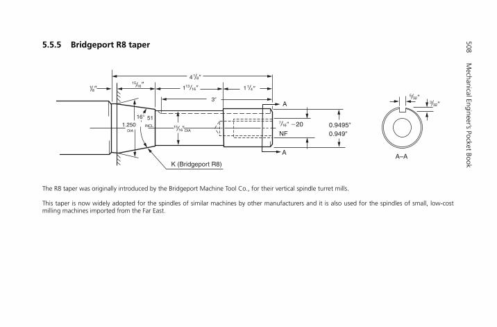
508M
echanical Engineer’s Pocket Book
1 1615
8��
1615 �
16
81
13 �
�
41 �1
1.2505116°
1
167 � �20
4
3�
DIA DIAINCL
A
0.9495�
0.949�
A
NF
K (Bridgeport R8)
325 �
323 �
A–A
5.5.5 Bridgeport R8 taper
The R8 taper was originally introduced by the Bridgeport Machine Tool Co., for their vertical spindle turret mills.
This taper is now widely adopted for the spindles of similar machines by other manufacturers and it is also used for the spindles of small, low-costmilling machines imported from the Far East.

Power Transmission 509
5.6 Fluid power transmission systems
Mechanical power transmission systems depend on such devices as shafts, universaljoints, gears, belts, chains, etc., to transmit energy and motion from one part of a systemto another. As such they tend to be relatively inflexible. Fluid power systems, although lessefficient in the use of energy, are extremely flexible and controllable. The following tablecompares electrical, hydraulic and pneumatic systems.
Comparisons of electrical, hydraulic and pneumatic systems
Electrical Hydraulic Pneumatic
Energy source Usually from outside Electric motor or Electric motor or supplier diesel driven diesel driven
Energy storage Limited (batteries) Limited (accumulator) Good (reservoir)
Distribution system Excellent, with Limited basically a Goodminimal loss local facility Can be treated as a plant
wide service
Energy cost Lowest Medium Highest
Rotary actuators AC and DC motors Low speed Wide speed rangeGood control on DC Good control Accurate speed control motors difficultAC motors cheap Can be stalled
Linear actuator Short motion via Cylinders CylinderssolenoidOtherwise via Very high force Medium forcemechanical conversion
Controllable force Possible with solenoid Controllable high Controllable medium and DC motors force forceComplicated by need for cooling
Points to note Danger from electric Leakage dangerous Noiseshock and unsightly
Fire hazard
Source: Table 1.1 in Hydraulics & Pneumatics, 2nd edn. Andrew Parr: B/Heinemann.
This section is concerned only with fluid power transmission, that is pneumatic (gases: usu-ally air) and hydraulic (liquids: mainly oil or water). The main advantages and disadvantagesof such systems arise out of the different characteristics of low density compressible gasesand (relatively) high density incompressible liquids. A pneumatic system, for example,tends to have a ‘softer’ action than a hydraulic system which is more positive. A pneumaticsystem also exhausts to the atmosphere and this simplifies the pipework since no returncircuit is required. A liquid-based hydraulic system can operate at much higher pressuresand can provide much higher forces. Hydraulic systems employ water as the operating fluidwhere large volumes are required as in operating the raising and lowering mechanism ofTower Bridge in London or in the lift bridges employed mainly on the canal systems andwaterways of continental Europe. However for most industrial purposes the hydraulic fluidis oil which is self-lubricating and does not cause corrosion.
H6508-Ch05.6.qxd 9/12/05 4:47 PM Page 509
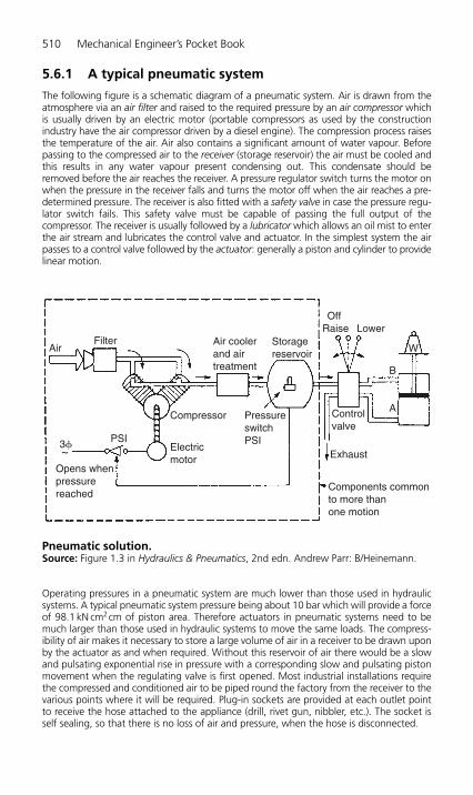
5.6.1 A typical pneumatic system
The following figure is a schematic diagram of a pneumatic system. Air is drawn from theatmosphere via an air filter and raised to the required pressure by an air compressor whichis usually driven by an electric motor (portable compressors as used by the constructionindustry have the air compressor driven by a diesel engine). The compression process raisesthe temperature of the air. Air also contains a significant amount of water vapour. Beforepassing to the compressed air to the receiver (storage reservoir) the air must be cooled andthis results in any water vapour present condensing out. This condensate should beremoved before the air reaches the receiver. A pressure regulator switch turns the motor onwhen the pressure in the receiver falls and turns the motor off when the air reaches a pre-determined pressure. The receiver is also fitted with a safety valve in case the pressure regu-lator switch fails. This safety valve must be capable of passing the full output of thecompressor. The receiver is usually followed by a lubricator which allows an oil mist to enterthe air stream and lubricates the control valve and actuator. In the simplest system the airpasses to a control valve followed by the actuator: generally a piston and cylinder to providelinear motion.
510 Mechanical Engineer’s Pocket Book
Compressor
Electricmotor
PSI
Opens whenpressurereached
B
W
A
Air coolerand airtreatment
PressureswitchPSI
FilterAir
Storagereservoir
Off Raise Lower
Controlvalve
Exhaust3�
Components commonto more thanone motion
~
Pneumatic solution.Source: Figure 1.3 in Hydraulics & Pneumatics, 2nd edn. Andrew Parr: B/Heinemann.
Operating pressures in a pneumatic system are much lower than those used in hydraulicsystems. A typical pneumatic system pressure being about 10 bar which will provide a forceof 98.1 kN cm2cm of piston area. Therefore actuators in pneumatic systems need to bemuch larger than those used in hydraulic systems to move the same loads. The compress-ibility of air makes it necessary to store a large volume of air in a receiver to be drawn uponby the actuator as and when required. Without this reservoir of air there would be a slowand pulsating exponential rise in pressure with a corresponding slow and pulsating pistonmovement when the regulating valve is first opened. Most industrial installations requirethe compressed and conditioned air to be piped round the factory from the receiver to thevarious points where it will be required. Plug-in sockets are provided at each outlet pointto receive the hose attached to the appliance (drill, rivet gun, nibbler, etc.). The socket isself sealing, so that there is no loss of air and pressure, when the hose is disconnected.
H6508-Ch05.6.qxd 9/12/05 4:47 PM Page 510
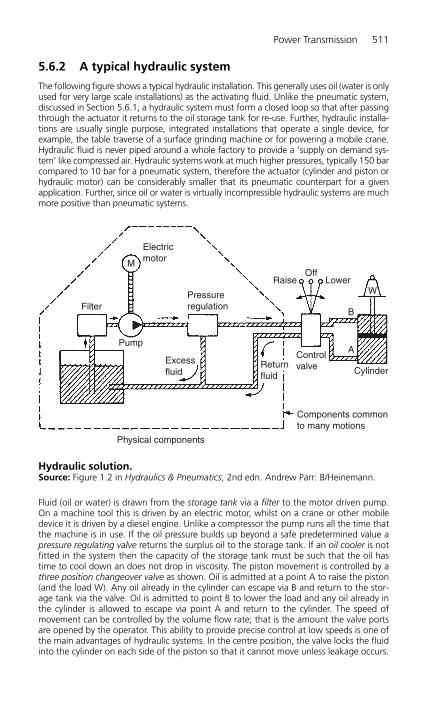
5.6.2 A typical hydraulic system
The following figure shows a typical hydraulic installation. This generally uses oil (water is onlyused for very large scale installations) as the activating fluid. Unlike the pneumatic system,discussed in Section 5.6.1, a hydraulic system must form a closed loop so that after passingthrough the actuator it returns to the oil storage tank for re-use. Further, hydraulic installa-tions are usually single purpose, integrated installations that operate a single device, forexample, the table traverse of a surface grinding machine or for powering a mobile crane.Hydraulic fluid is never piped around a whole factory to provide a ‘supply on demand sys-tem’ like compressed air. Hydraulic systems work at much higher pressures, typically 150 barcompared to 10 bar for a pneumatic system, therefore the actuator (cylinder and piston orhydraulic motor) can be considerably smaller that its pneumatic counterpart for a givenapplication. Further, since oil or water is virtually incompressible hydraulic systems are muchmore positive than pneumatic systems.
Fluid (oil or water) is drawn from the storage tank via a filter to the motor driven pump.On a machine tool this is driven by an electric motor, whilst on a crane or other mobiledevice it is driven by a diesel engine. Unlike a compressor the pump runs all the time thatthe machine is in use. If the oil pressure builds up beyond a safe predetermined value apressure regulating valve returns the surplus oil to the storage tank. If an oil cooler is notfitted in the system then the capacity of the storage tank must be such that the oil hastime to cool down an does not drop in viscosity. The piston movement is controlled by athree position changeover valve as shown. Oil is admitted at a point A to raise the piston(and the load W). Any oil already in the cylinder can escape via B and return to the stor-age tank via the valve. Oil is admitted to point B to lower the load and any oil already inthe cylinder is allowed to escape via point A and return to the cylinder. The speed ofmovement can be controlled by the volume flow rate; that is the amount the valve portsare opened by the operator. This ability to provide precise control at low speeds is one ofthe main advantages of hydraulic systems. In the centre position, the valve locks the fluidinto the cylinder on each side of the piston so that it cannot move unless leakage occurs.
Power Transmission 511
Electricmotor
Pressureregulation
Excess fluid
Pump
Filter
Returnfluid
Controlvalve
Components commonto many motions
Physical components
RaiseOff
Lower
Cylinder
A
B
W
M
Hydraulic solution.Source: Figure 1.2 in Hydraulics & Pneumatics, 2nd edn. Andrew Parr: B/Heinemann.
H6508-Ch05.6.qxd 9/12/05 4:47 PM Page 511

The regulator bypasses the excess oil still being pumped back to the storage tank. Whenoil is used as the actuating fluid the system is self-lubricating.
For large scale systems, particularly when using water to reduce costs, very large volumesof water are required at very high pressures for example when raising and lowering TowerBridge in London. Since this operation is only required at relatively infrequent intervals itwould be uneconomical to employ a pump big enough to drive the operating ramsdirectly. The solution is to install a hydraulic accumulator as shown in following figurebetween the pump and the operating valve and rams. The hydraulic accumulator consistsof a large cylinder and ram carrying a heavy mass to provide the required pressure. Thesize of the cylinder and ram depends on the volume of fluid required to operate the actu-ating rams of (in this example) the bridge. The pressure is controlled by the mass bearingdown on the accumulator. A relatively small and economic pump providing the hydraulicfluid at the required pressure but at a low delivery volume rate is used to raise the accu-mulator when the system is not being used. The accumulator, alone, provides the pres-sure fluid on demand to actuate the operating rams.
512 Mechanical Engineer’s Pocket Book
K
H
F
EDA
T
Accumulator
Hydraulicpump
Press
B
C
Water is forced by a pump past the valve A into the cylinder B. This raises the heavilyloaded ram C. Meantime valve D is closed. The water cannot escape from B by the valveA, for the pressure upon the top closes it. So water under pressure is stored in the accu-mulator. When it is desired to work the press the valve D is opened and the water isforced from cylinder B into E. This raises the ram F, and compresses the bale of cotton,or whatever it may be, between the faces H and K.
Hydraulic press and accumulator.
H6508-Ch05.6.qxd 9/12/05 4:47 PM Page 512
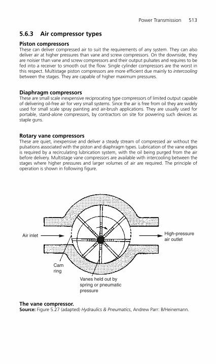
5.6.3 Air compressor types
Piston compressorsThese can deliver compressed air to suit the requirements of any system. They can alsodeliver air at higher pressures than vane and screw compressors. On the downside, theyare noisier than vane and screw compressors and their output pulsates and requires to befed into a receiver to smooth out the flow. Single cylinder compressors are the worst inthis respect. Multistage piston compressors are more efficient due mainly to intercoolingbetween the stages. They are capable of higher maximum pressures.
Diaphragm compressorsThese are small scale inexpensive reciprocating type compressors of limited output capableof delivering oil-free air for very small systems. Since the air is free from oil they are widelyused for small scale spray painting and air-brush applications. They are usually used forportable, stand-alone compressors, by contractors on site for powering such devices as staple guns.
Rotary vane compressorsThese are quiet, inexpensive and deliver a steady stream of compressed air without thepulsations associated with the piston and diaphragm types. Lubrication of the vane edgesis required by a recirculating lubrication system, with the oil being purged from the airbefore delivery. Multistage vane compressors are available with intercooling between thestages where higher pressures and larger volumes of air are required. The principle ofoperation is shown in following figure.
Power Transmission 513
Camring
Vanes held out byspring or pneumaticpressure
High-pressureair outlet
Air inlet
The vane compressor.Source: Figure 5.27 (adapted) Hydraulics & Pneumatics, Andrew Parr: B/Heinemann.
H6508-Ch05.6.qxd 9/12/05 4:47 PM Page 513
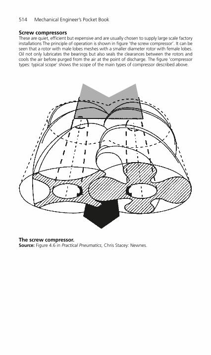
514 Mechanical Engineer’s Pocket Book
The screw compressor.Source: Figure 4.6 in Practical Pneumatics, Chris Stacey: Newnes.
Screw compressorsThese are quiet, efficient but expensive and are usually chosen to supply large scale factoryinstallations The principle of operation is shown in figure ‘the screw compressor’. It can beseen that a rotor with male lobes meshes with a smaller diameter rotor with female lobes.Oil not only lubricates the bearings but also seals the clearances between the rotors andcools the air before purged from the air at the point of discharge. The figure ‘compressortypes: typical scope’ shows the scope of the main types of compressor described above.
H6508-Ch05.6.qxd 9/12/05 4:47 PM Page 514
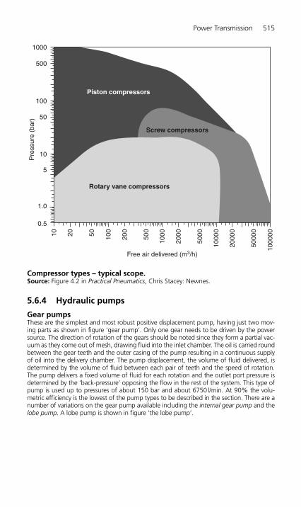
5.6.4 Hydraulic pumps
Gear pumpsThese are the simplest and most robust positive displacement pump, having just two mov-ing parts as shown in figure ‘gear pump’. Only one gear needs to be driven by the powersource. The direction of rotation of the gears should be noted since they form a partial vac-uum as they come out of mesh, drawing fluid into the inlet chamber. The oil is carried roundbetween the gear teeth and the outer casing of the pump resulting in a continuous supplyof oil into the delivery chamber. The pump displacement, the volume of fluid delivered, isdetermined by the volume of fluid between each pair of teeth and the speed of rotation.The pump delivers a fixed volume of fluid for each rotation and the outlet port pressure isdetermined by the ‘back-pressure’ opposing the flow in the rest of the system. This type ofpump is used up to pressures of about 150 bar and about 6750 l/min. At 90% the volu-metric efficiency is the lowest of the pump types to be described in the section. There are anumber of variations on the gear pump available including the internal gear pump and thelobe pump. A lobe pump is shown in figure ‘the lobe pump’.
Power Transmission 515
10
10
20 50
50
100
100
200
500
500
1000
1000
2000
5000
1000
0
2000
0
5000
0
1000
00
Free air delivered (m3/h)
Rotary vane compressors
Screw compressors
Piston compressors
5
1.0
0.5
Pre
ssur
e (b
ar)
Compressor types – typical scope.Source: Figure 4.2 in Practical Pneumatics, Chris Stacey: Newnes.
H6508-Ch05.6.qxd 9/12/05 4:47 PM Page 515
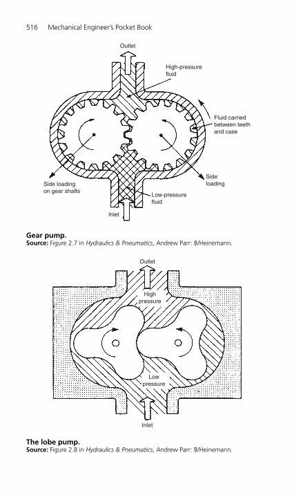
516 Mechanical Engineer’s Pocket Book
Outlet
High-pressurefluid
Fluid carriedbetween teethand case
Sideloading
Low-pressurefluid
Inlet
Side loadingon gear shafts
Gear pump.Source: Figure 2.7 in Hydraulics & Pneumatics, Andrew Parr: B/Heinemann.
Outlet
Lowpressure
Inlet
Highpressure
The lobe pump.Source: Figure 2.8 in Hydraulics & Pneumatics, Andrew Parr: B/Heinemann.
H6508-Ch05.6.qxd 9/12/05 4:47 PM Page 516
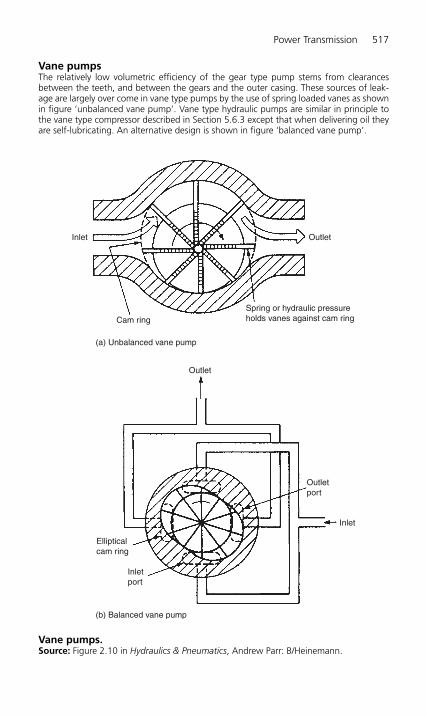
Power Transmission 517
Vane pumpsThe relatively low volumetric efficiency of the gear type pump stems from clearancesbetween the teeth, and between the gears and the outer casing. These sources of leak-age are largely over come in vane type pumps by the use of spring loaded vanes as shownin figure ‘unbalanced vane pump’. Vane type hydraulic pumps are similar in principle tothe vane type compressor described in Section 5.6.3 except that when delivering oil theyare self-lubricating. An alternative design is shown in figure ‘balanced vane pump’.
Inlet
Cam ring
Outlet
Outletport
Inlet
Inletport
Ellipticalcam ring
(b) Balanced vane pump
(a) Unbalanced vane pump
Spring or hydraulic pressureholds vanes against cam ring
Outlet
Vane pumps.Source: Figure 2.10 in Hydraulics & Pneumatics, Andrew Parr: B/Heinemann.
H6508-Ch05.6.qxd 9/12/05 4:47 PM Page 517

Piston pumpsReciprocating force pumps are only used on very large scale applications in conjunction withan accumulator to smooth out the pulsations. Nowadays, for most applications requiringmultiple piston pumps, the pistons and cylinders are arranged radially as shown in figure‘radial piston pump’. The pump consists of several hollow pistons inside a stationary cylin-der block. Each piston has spring loaded inlet and outlet valves. As the cam rotates, fluid istransferred relatively smoothly from the inlet port to the outlet port. The pump shown in fig-ure ‘piston pump with stationary can and rotating block’ is similar in principle but uses a sta-tionary cam and a rotating cylinder block. This arrangement removes the need for multipleinlet and outlet valves and is consequently more simple, reliable and cheaper to manufac-ture and maintain, hence this is the more commonly used type.
518 Mechanical Engineer’s Pocket Book
Fixedcasing
Outlet
Rotating cam
Slidingpiston
Outlet valves
Inlet valves
Inlet
Fixedcylinderblock
Radial piston pump.
H6508-Ch05.6.qxd 9/12/05 4:47 PM Page 518
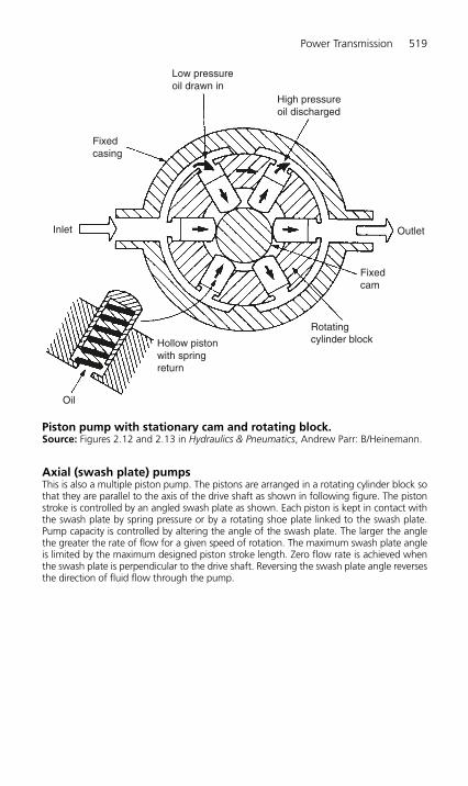
Power Transmission 519
Axial (swash plate) pumpsThis is also a multiple piston pump. The pistons are arranged in a rotating cylinder block sothat they are parallel to the axis of the drive shaft as shown in following figure. The pistonstroke is controlled by an angled swash plate as shown. Each piston is kept in contact withthe swash plate by spring pressure or by a rotating shoe plate linked to the swash plate.Pump capacity is controlled by altering the angle of the swash plate. The larger the anglethe greater the rate of flow for a given speed of rotation. The maximum swash plate angleis limited by the maximum designed piston stroke length. Zero flow rate is achieved whenthe swash plate is perpendicular to the drive shaft. Reversing the swash plate angle reversesthe direction of fluid flow through the pump.
Low pressureoil drawn in
Fixedcasing
High pressureoil discharged
Rotatingcylinder blockHollow piston
with springreturn
Oil
Fixedcam
OutletInlet
Piston pump with stationary cam and rotating block.Source: Figures 2.12 and 2.13 in Hydraulics & Pneumatics, Andrew Parr: B/Heinemann.
H6508-Ch05.6.qxd 9/12/05 4:47 PM Page 519

All types of piston pumps have very high volumetric efficiency and can be used at thehighest hydraulic pressures. They are more complex than vane and gear pumps and are,therefore more expensive in first cost and to maintain. The following table compares theadvantages and limitations of various types of hydraulic pumps.
Comparison of hydraulic pump types
Type Maximum Maximum Variable Positive pressure (bar) flow (l/min) displacement displacement
Centrifugal 20 3000 No NoGear 175 300 No YesVane 175 500 Yes YesAxial piston (port-plate) 300 500 Yes YesAxial piston (valved) 700 650 Yes YesIn-line piston 1000 100 Yes Yes
Specialist pumps are available for pressures up to about 7000 bar at low flows. The delivery from cen-trifugal and gear pumps can be made variable by changing the speed of the pump motor with a vari-able frequency (VF) drive.Source: Table 2.1 in Hydraulics & Pneumatics, Andrew Parr: B/Heinemann.
520 Mechanical Engineer’s Pocket Book
Shoe plate
Angled circular swash plate
Input shaft
Shoe plate
Swash plate
Drive shaft
Swash angledetermines stroke
Cylinderblock
Fixedblock
Piston
Outlet
Inlet
Pistons stroked by ballsmoving on swash plate
Axial pump with swash plate.Source: Figure 2.14 in Hydraulics & Pneumatics, Andrew Parr: B/Heinemann.
H6508-Ch05.6.qxd 9/12/05 4:47 PM Page 520
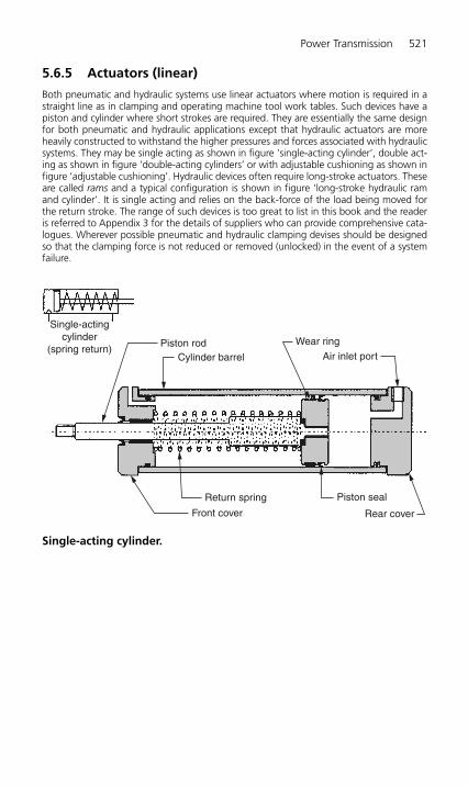
Power Transmission 521
5.6.5 Actuators (linear)
Both pneumatic and hydraulic systems use linear actuators where motion is required in astraight line as in clamping and operating machine tool work tables. Such devices have apiston and cylinder where short strokes are required. They are essentially the same designfor both pneumatic and hydraulic applications except that hydraulic actuators are moreheavily constructed to withstand the higher pressures and forces associated with hydraulicsystems. They may be single acting as shown in figure ‘single-acting cylinder’, double act-ing as shown in figure ‘double-acting cylinders’ or with adjustable cushioning as shown infigure ‘adjustable cushioning’. Hydraulic devices often require long-stroke actuators. Theseare called rams and a typical configuration is shown in figure ‘long-stroke hydraulic ramand cylinder’. It is single acting and relies on the back-force of the load being moved forthe return stroke. The range of such devices is too great to list in this book and the readeris referred to Appendix 3 for the details of suppliers who can provide comprehensive cata-logues. Wherever possible pneumatic and hydraulic clamping devises should be designedso that the clamping force is not reduced or removed (unlocked) in the event of a systemfailure.
Single-actingcylinder
(spring return)Piston rod
Cylinder barrel
Return spring Piston seal
Rear coverFront cover
Wear ring
Air inlet port
Single-acting cylinder.
H6508-Ch05.6.qxd 9/12/05 4:47 PM Page 521
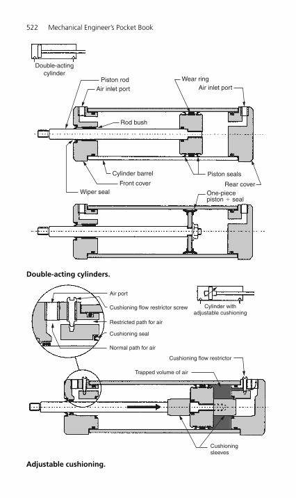
522 Mechanical Engineer’s Pocket Book
Air port
Cushioning flow restrictor screw
Cushioning flow restrictor
Cushioningsleeves
Trapped volume of air
Restricted path for air
Cushioning seal
Cylinder withadjustable cushioning
Normal path for air
Adjustable cushioning.
Double-actingcylinder
Piston rodAir inlet port
Piston seals
Rear coverOne-piecepiston � seal
Rod bush
Cylinder barrel
Front coverWiper seal
Wear ringAir inlet port
Double-acting cylinders.
H6508-Ch05.6.qxd 9/12/05 4:47 PM Page 522
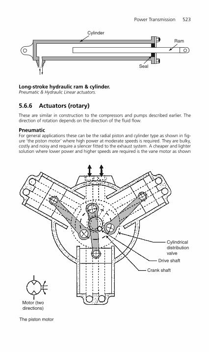
Power Transmission 523
5.6.6 Actuators (rotary)
These are similar in construction to the compressors and pumps described earlier. Thedirection of rotation depends on the direction of the fluid flow.
PneumaticFor general applications these can be the radial piston and cylinder type as shown in fig-ure ‘the piston motor’ where high power at moderate speeds is required. They are bulky,costly and noisy and require a silencer fitted to the exhaust system. A cheaper and lightersolution where lower power and higher speeds are required is the vane motor as shown
Cylinder
Seal
Ram
Long-stroke hydraulic ram & cylinder.Pneumatic & Hydraulic Linear actuators.
Motor (twodirections)
The piston motor
Crank shaft
Drive shaft
Cylindricaldistributionvalve
H6508-Ch05.6.qxd 9/12/05 4:47 PM Page 523
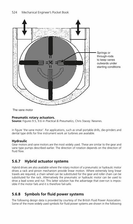
in figure ‘the vane motor’. For applications, such as small portable drills, die-grinders anddental type drills for fine instrument work air turbines are available.
HydraulicGear motors and vane motors are the most widely used. These are similar to the gear andvane type pumps described earlier. The direction of rotation depends on the direction offluid flow.
5.6.7 Hybrid actuator systems
Hybrid drives are also available where the rotary motion of a pneumatic or hydraulic motordrives a rack and pinion mechanism provide linear motion. Where extremely long lineartravels are required, a chain wheel can be substituted for the gear and roller chain can besubstituted for the rack. Alternatively the pneumatic or hydraulic motor can be used todrive a lead screw and nut. This latter solution has the advantage that over-run is impos-sible if the motor fails and it is therefore fail-safe.
5.6.8 Symbols for fluid power systems
The following design data is provided by courtesy of the British Fluid Power Association.Some of the more widely used symbols for fluid power systems are shown in the following
524 Mechanical Engineer’s Pocket Book
Pneumatic rotary actuators.Source: Figures 9.5, 9.6 in Practical & Pneumatics, Chris Stacey: Newnes.
The vane motor
Springs orthrough-rodsto keep vanesoutwards understarting conditions
H6508-Ch05.6.qxd 9/12/05 4:47 PM Page 524
Power Transmission 525
Source of energy –Hydraulic
Source of energy – Pneumatic
Hydraulic pump Fixed displacement One flow direction
Hydraulic pump Variable displacement Two flow directions
Hydraulic motor Fixed displacement One flow direction
Hydraulic motor Variable displacement Two flow directions ofrotation
Air compressor
Pneumatic motor Fixed displacement One flow direction
Accumulator – Gas loaded
Air receiver
Hydraulic cylinder – Double-acting
Pneumatic cylinder – Double-acting
Cylinder– Double-acting– Double-endedPiston rod Hydraulic
Pneumatic cylinder– Single-acting– Spring return
Cylinder– Double-acting– Adjustable cushions
both ends Pneumatic
Pressure intensifier– Single fluid– Hydraulic
Semi-rotary actuator– Double-acting– Hydraulic
Semi-rotary actuator– Single-acting– Spring return– Pneumatic
Telescopic cylinder– Double-acting– Hydraulic
Electric motor (from IEC 617)
Hydraulic and pneumatic symbols.
Symbol Description Symbol Description
H6508-Ch05.6.qxd 9/12/05 4:47 PM Page 525
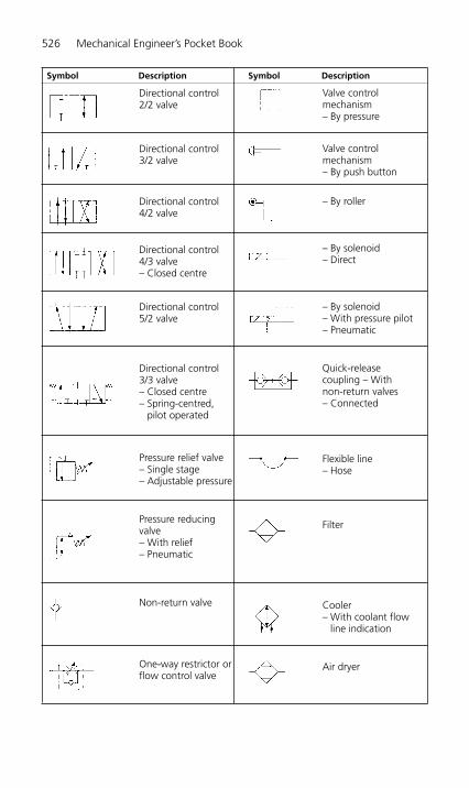
526 Mechanical Engineer’s Pocket Book
Directional control 2/2 valve
Directional control 3/2 valve
Directional control 4/2 valve
Directional control 4/3 valve– Closed centre
Directional control 5/2 valve
Directional control 3/3 valve– Closed centre– Spring-centred,
pilot operated
Pressure relief valve– Single stage– Adjustable pressure
Pressure reducingvalve– With relief– Pneumatic
Non-return valve
One-way restrictor orflow control valve
Valve control mechanism– By pressure
Valve control mechanism– By push button
– By roller
– By solenoid– Direct
– By solenoid– With pressure pilot– Pneumatic
Quick-release coupling – With non-return valves – Connected
Flexible line– Hose
Filter
Cooler– With coolant flow
line indication
Air dryer
Symbol Description Symbol Description
H6508-Ch05.6.qxd 9/12/05 4:48 PM Page 526

Power Transmission 527
figure. For the full range of graphic symbols the reader is referred to ISO 1219-1 asamended in 1991. For the rules relating to circuit layout see ISO 1219-2. For port identi-fication and operator marking see ISO 9461 (hydraulic) or CETOP RP68P (pneumatic) orISO 5599 (pneumatic).
5.6.9 Fluid power transmission design data (general formulae)
Hydraulic(a) Pumps and motors
Flow rate (l/min)
Shaft torque (Nm)
Shaft power (kW)
Hydraulic power (kW)
For a quick calculation
(b) Cylinders
Pressure (N/m2)
Flow rate (l/min) Q � 60.A.v.103
F � force (N)A � area (m2)v � velocity (m/s)p � pressure (bar)D � displacement (cm3/rev)n � rev/min
pFA
�
Power (kW) P tonnes mm/sec100
� �
PQ p
� �
600
PT n
� �
9554
TD p
� �
20p
QD n
� �
1000
H6508-Ch05.6.qxd 9/12/05 4:48 PM Page 527

(c) Flow
Flow (l/min)
�p � pressure change (bar)
That is, if you double the flow you get 4 times the pressure change
Pressure loss in pipes
This chart gives the approximate pressure drop in smooth bore straight pipes, in bar per 3 m length.Bends and fittings will increase the above pressure losses and manufacturers should be consulted formore accurate figures.
Pneumatic(a) Flow through pipes
where:�p � pressure drop (bar)Q � free air flow (m3/s) � l/s � 10�3
L � pipe length (m)d � internal diameter of pipe
(b) Velocity through pipes
vQ
p d�
�
1273
( 1) 2
� �� � � � �
�
� �
pL
d p
1.6 10 (Q 10 ) 108 3 1.85 3
5
Flow in Tube bore size (mm)l/min 5 7 10 13 16 21 25 30 36
1 0.69 0.222 1.38 0.443 2.07 0.66 0.175 4.14 1.24 0.247.5 6.55 1.72 0.31
10 3.10 0.38 0.1415 5.38 0.69 0.21 0.0820 1.10 0.30 0.1430 2.21 0.69 0.25 0.0440 1.17 0.45 0.08 0.0450 0.59 0.12 0.07 0.0375 1.31 0.23 0.14 0.06 0.02
100 0.41 0.22 0.13 0.03150 0.45 0.23 0.06200 0.41 0.10250 0.16
Q p� �
528 Mechanical Engineer’s Pocket Book
H6508-Ch05.6.qxd 9/12/05 4:48 PM Page 528

Power Transmission 529
where:v � flow velocity (m/s)p � initial pressure (bar)d � inside pipe diameter (mm)
If the free air flow is known, the minimum inside diameter to keep velocity below 6 m/s,can be found from:
For normal installations, where the pressure is about seven bar gauge, this can be simpli-fied to:
d (mm) should be greater than
Source: Pages 14 &15 BFPA Data books.
5.6.10 Fluid power transmission design data (hydraulic cylinders)
Output force and maximum rod lengthsExample: Knowing the output force required (200 kN) and the pressure of the system(160 bar), connect Output force through pressure to cut cylinder diameter.
Answer: 125 mm.
To find the maximum length of a piston rod. Connect output force required (200 kN)through rod diameter (70 mm) to cut the maximum rod length scale; this gives you the(Lm) dimensions.
Answer: 2800 mm.
To find the actual length stroke (LA) for a specific mounting use formulae below.
Maximum stroke lengths for specific mounting casesFoot mounted, eye rod end ............................ LA � Lm � 0.8Foot mounted, rigidly supported rod .............. LA � LmFront flange, eye rod end ............................... LA � Lm � 0.8Front flange, rigidly supported rod ................ LA � LmRear flange, eye rod end ................................ LA � Lm � 0.4Real flange, rigidly supported rod ................... LA � Lm � 0.8Rear eye, eye rod end ..................................... LA � Lm � 0.3Trunnion head end, eye rod end ..................... LA � Lm � 0.3Trunnion gland end, eye rod end .................... LA � Lm � 0.6Trunnion gland end, rigidly supported end ..... LA � Lm � 0.8
For intermediate trunnion positions scaled multiplier factors must be taken. Clevis andspherical eye mountings have the same factor as eye mountings.
Example: Having found Lm (2800 mm) for rear flange mount with eye rod endLA � Lm � 0.4 � 2800 � 0.4 � 1120 mm.
5 � Q
d (mm)212( 1)
��
�
Qp
H6508-Ch05.6.qxd 9/12/05 4:48 PM Page 529
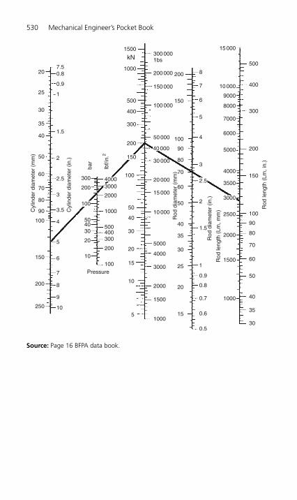
530 Mechanical Engineer’s Pocket Book
20
1500
1000200
150
10 000
15 000
9000
8000
7000
6000
5000
4000
3500
2500
1500
1000
3000
2000
100
90
80
70
60
50
40
35
25
1535
30
40
50
60
70
80
90
100
200
300
400
500
150
30
20
500
400
300
200
150
50
40
30
20
15
10
51000
0.5
0.6
0.7
0.8
0.9
1
1.5
3
4
5
6
7
1500
2000
3000
4000
5000
10 000
20 000
30 000
40 000
50 000
100 000
200 000
300 0001bs
150 000
15 000
100
kN7.50.8
0.9
1
2
2.5
Cyl
inde
r di
amet
er (
mm
)
Rod
dia
met
er (
mm
)
Rod
dia
met
er (
in.)
Rod
leng
th (
Lm, m
m) R
od le
ngth
(Lm
, in.
)
Cyl
inde
r di
amet
er (
in.)
3
40003000
2000
1000
500400300
200
100
4
5
6
7
8
9
10
3.5
1.5
30
40
50
60300
bar
lbf/i
n.2
200
100
504030
20
10
Pressure
70
80
90
100
150
250
200
25
35
2.5
2
8
Source: Page 16 BFPA data book.
H6508-Ch05.6.qxd 9/12/05 4:48 PM Page 530
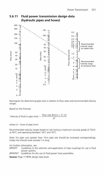
Power Transmission 531
5.6.11 Fluid power transmission design data (hydraulic pipes and hoses)
Nomogram for determining pipe sizes in relation to flow rates and recommended velocityranges.
Based on the formula:
where d � bore of pipe (mm)
Recommended velocity ranges based on oils having a maximum viscosity grade of 70cStat 40°C and operating between 18°C and 70°C.
Note: For pipe runs greater than 10 m pipe size should be increased correspondingly.Intake line should never exceed 1 m long.
For further information, see:BFPA/P7 Guidelines to the selection and application of tube couplings for use in fluid
power systems.BFPA/P47 Guidelines for the use of fluid power hose assemblies.
Source: Page 17 BFPA design data book.
Velocity of fluid in pipe (m/s)Flow rate (
�ll/min) 21.22
2
�
d
400
300
200
150
150
100
50
40
30
20
15
1098765
4
32.5
100
50
40
30
20
15
1098765
4
3
2
Flo
w (
l/min
)
Bor
e (m
m)
Flo
w–v
eloc
ity (
m/s
)
0.3
0.4
0.50.60.70.80.9
1.5
Recommendedvelocity rangefor intake lines
Recommendedvelocity rangefor pressure lines
1
2
3
4
56789
10
H6508-Ch05.6.qxd 9/12/05 4:48 PM Page 531

5.6.12 Fluid power transmission design data (hydraulic fluids, seals and contamination control)
Fluids
ISO Classification of Hydraulic Fluids – BS ISO 6743-4HH Non inhibited refined mineral oilsHL Refined mineral oils with improved anti-rust and anti-oxidation propertiesHM Oils of HL type with improved anti-wear propertiesHV Oils of HM type with improved viscosity/temperature propertiesHFAE Oil in water emulsionsHFAS Chemical solutions in waterHFB Water-in-oil emulsionsHFC Water polymer solutionsHFDR Synthetic fluids of the phosphate ester type
Ecologically acceptable hydraulic fluidsHETG TryglyceridesHEPG PolyglycolsHEES Synthetic EstersHEPR Polyalphaclefins
Viscosity Classification of Hydraulic Fluids – ISO 3448 (BS 4231)Each viscosity grade is designated by the nearest whole number to its mid-point kinematicviscosity in centistokes at 40°C. It is abbreviated ISOVG … Common viscosity grades ofhydraulic fluids are VG5, 10, 22, 32, 46, 68, 100, 150, 220 and 320.
Thus HM32 is a mineral oil with improved anti-rust, anti-oxidation and anti-wear proper-ties having a viscosity of approximately 32 centistokes at 40°C.
For further details of specific fluids see BFPA/P12, Mineral oil data sheets and BFPA/P13, Fireresistant fluids data sheets, BFPA/P67 Ecologically acceptable hydraulic fluids data sheets.
SealsSeal material Recommended forAcrylonitrile butadiene (NBR) air, oil, water, water/glycolPolyacrylate rubber (ACM) air, oilPolyurethane (AU, EU) air, oilFluorocarbon rubber (FKM) air, oil water, water/glycol, chlorinated hydro-
carbons, triaryl phosphatesSilicone (VOM) air, oil, chlorinated hydrocarbonsStyrene Butadiene (SBR) air, water, water/glycolEthylene propylene diene (EPDM) air, water, water/glycol, phosphate esterPolytetrafluorethylene (PTFE) air, oil, water, water/glycol, phosphate ester
For full details of seal compatibilities, see ISO 6072: Hydraulic fluid power, compatibilitybetween elastomeric materials and fluids or BS 7714: Guide for care and handling of sealsfor fluid power applications. For recommendation of O-ring seal standards, see BFPA/P22‘Industrial O-ring Standards – Metric vs Inch.’
Source: Pages 18–20 inclusive, BFPA data book.
Fluid cleanlinessThe presence of particulate contamination (‘dirt’) is the single most important factor gov-erning the life and reliability of fluid power systems. Operating with clean fluids is essen-tial. Advice on contamination control can be gained from guide line document BFPA/P5.
532 Mechanical Engineer’s Pocket Book
H6508-Ch05.6.qxd 9/12/05 4:48 PM Page 532

Power Transmission 533
Contamination control
Specification of Degree of Filtration – ISO 4572 (BS 6275/1)The multipass test, ISO 4572 (BS 6275/1), was introduced to overcome the difficulties incomparing the performance of filters. The element is subjected to a constant circulationof oil during which time fresh contaminant (ISO Test Dust) is injected into the test rig. Thecontaminant that is not removed by the element under test is recirculated thereby simu-lating service conditions.
The filtration ratio of the filter is obtained by the analysis of fluid samples extracted fromupstream and downstream of the test filter, thus
The rating of a filter element is stated as the micrometer size where �x is a high value (e.g.100 or 200)
Fluid cleanliness standardsThe preferred method of quoting the number of solid contaminant particles in a sampleis the use of BS ISO 4406.
The code is constructed from the combination of two range numbers selected from thefollowing table. The first range number represents the number of particles in a millilitresample of the fluid that are larger than 5 m, and the second number represents thenumber of particles that are larger than 15 m.
b xx
�number of particles larger than upstreaam of the filter
number of particles larger than downstream of the filterx
Number of particles per millilitreScale number
More than up to and including
10 000 20 000 215 000 10 000 202 500 5000 191 300 2500 18
640 1300 17320 640 16160 320 1580 160 1440 80 1320 40 1210 20 115 10 102.5 5 91.3 2.5 80.64 1.3 7
For example code 18/13 indicates that there are between 1300 and 2500 particles largerthan 5 m and between 40 and 80 particles larger than 15 m.
For further details and comparisons of ISO 4406 with other cleanliness classes, seeBFPA/P5 – Guidelines to contamination control in fluid power systems.
H6508-Ch05.6.qxd 9/12/05 4:48 PM Page 533
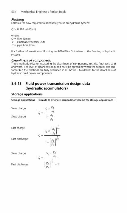
FlushingFormula for flow required to adequately flush an hydraulic system:
Q � 0.189 vd (l/min)
where:Q � flow (l/min)v � kinematic viscosity (cSt)d � pipe bore (mm)
For further information on flushing see BFPA/P9 – Guidelines to the flushing of hydraulicsystems.
Cleanliness of componentsThree methods exist for measuring the cleanliness of components: test rig, flush test, stripand wash. The level of cleanliness required must be agreed between the supplier and cus-tomer but the methods are fully described in BFPA/P48 – Guidelines to the cleanliness ofhydraulic fluid power components.
5.6.13 Fluid power transmission design data (hydraulic accumulators)
Storage applications
Storage applications Formula to estimate accumulator volume for storage applications
V
Vp
p
p
p
1
a3
1
2
11.4
�
�
3 1⎛
⎝
⎜⎜⎜⎜⎜
⎞
⎠
⎟⎟⎟⎟⎟⎟−
Slow charge
Fast discharge
V
Vp
p
p
p
1
a2
1
3
�
�⎛
⎝
⎜⎜⎜⎜⎜
⎞
⎠
⎟⎟⎟⎟⎟⎟
−⎛
⎝
⎜⎜⎜⎜⎜
⎞
11 4
21
.
⎠⎠
⎟⎟⎟⎟⎟⎟
11.4
Fast charge
Fast discharge
V
Vp
p
p
p
1
a2
1
2
3
1
�
�
�
Slow charge
Slow charge
534 Mechanical Engineer’s Pocket Book
H6508-Ch05.6.qxd 9/12/05 4:48 PM Page 534
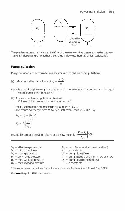
Power Transmission 535
The precharge pressure is chosen to 90% of the min. working pressure. n varies between1 and 1.4 depending on whether the charge is slow (isothermal) or fast (adiabatic).
Pump pulsation
Pump pulsation and Formula to size accumulator to reduce pump pulsations.
(a)
Note: It is good engineering practice to select an accumulator with port connection equalto the pump port connection.
(b) To check the level of pulsation obtained.Volume of fluid entering accumulator � D � C
For pulsation damping precharge pressure P1 � 0.7 � P2and assuming change from P1 to P2 is isothermal, then V2 � 0.7 � V1
V3 � V2 � (D � C)
Hence: Percentage pulsation above and below mean is
V1 � effective gas volume Va � V3 � V2 � working volume (fluid)V2 � min. gas volume k � a constant*V3 � max. gas volume Q � pump flow (l/min)p1 � pre charge pressure n � pump speed (rpm) if n � 100 use 100p2 � min. working pressure D � pump displacement (l/rev)p3 � max. working pressure C � a constant*
* Dependent on no. of pistons. For multi-piston pumps �3 pistons. k � 0.45 and C � 0.013.
Source: Page 21 BFPA data book.
P P
P2 3
2
100�⎛
⎝
⎜⎜⎜⎜⎜
⎞
⎠
⎟⎟⎟⎟⎟⎟
P PV
V3 32
3
1.4
�⎛
⎝
⎜⎜⎜⎜⎜
⎞
⎠
⎟⎟⎟⎟⎟⎟
Minimum effective volume (l) 1Vk Q
n�
�
P1 P2
P3
Useablevolume of
fluid
H6508-Ch05.6.qxd 9/12/05 4:48 PM Page 535

5.6.14 Fluid power transmission design data (hydraulic cooling and heating)
CoolingThe tank cools the oil through radiation and convection.
where:k � 12 at normally ventilated space
24 W/m2 °C at forced ventilation6 at poor air circulation
Required volume of water flow through the cooler:
HeatingHeating is most necessary if the environmental temperature is essentially below 0°C.
Requisite heating effect:
Energy
J � M � C � �T
where:M � Mass (kg)C � Specific heat capacity J/kg°C�T1 � temperature difference (°C) fluid/air�T2 � increase in fluid temperature (°C)�t � time (min)Note: 1 MJ � 0.2777 kW/h.
Heat equivalent of hydraulic power
Change of volume at variation of temperature
Change or volume �V � 6.3 � 10�4 � V � �T
Change of pressure at variation of temperatureNote: With an infinite stiff cylinder.Change of pressure �p � 11.8 � �T (in general, affected by many variables)
kJ/sflow (l/min) pressure (bar)
600kW�
��
PV T
t�
� �
� �2
35in kW
QT
� ��
860power loss
water1/h
PT A k
�� � �1
1000
536 Mechanical Engineer’s Pocket Book
H6508-Ch05.6.qxd 9/12/05 4:48 PM Page 536

Power Transmission 537
Example: The temperature variation of the cylinder oil from nighttime (10°C) to daytime/solar radiation (50°C) gives:
�P � 11.8 � 40 � 472 bar
Key
�T � temperature change (°C)P � power (kW)k � heating coefficient (W/m2 °C)A � area of tank excluding base (m2)�t � time change (min)�p � change in pressure (bar)C � specific heat capacity (J/kg°C)V � volume (l)
Source: Page 22 BFPA data book.
5.6.15 Fluid power transmission design data (pneumatic valve flow)
Valve flow performance is usually indicated by a flow factor of some kind, such as ‘C’, ‘b’,‘Cv’, ‘Kv’, and others.
The most accurate way of determining the performance of a pneumatic valve is throughits values of ‘C’ (conductance) and ‘b’ (critical pressure ratio).
These figures are determined by testing the valve to the CETOP RP50P recommendations.
The tests will result typically in a set of curves as shown below.
From these the critical pressure ratio ‘b’ can be found. ‘b’ represents the ratio of P2 to P1at which the flow velocity goes sonic (the limiting speed of air). Also the conductance ‘C’which represents the flow ‘dm3/s /bar absolute’ at this point.
If a set of curves are not available the value of flow for other pressure drops can be cal-culated from:
where:P1 � upstream pressure barC � conductance dm3/s/bar aQ � flow dm3/sP2 � downstream pressure barb � critical pressure ratio
Q CP
P
Pb
b� �
�
�1
2
1
2
11
⎡
⎣
⎢⎢⎢⎢⎢
⎤
⎦
⎥⎥⎥⎥⎥
H6508-Ch05.6.qxd 9/12/05 4:48 PM Page 537

ISO 6538/CETOP RP50P method
Source: Page 23 (part) BFPA data book.
5.6.16 Fluid power transmission design data (pneumatic cylinders)
Some factors to consider when selecting and using pneumatic linear actuators, air cylinders
Mode of actionThree basic types
● Single-acting, spring return: Movement and force by air pressure in one direction,return movement by internal spring force, usually sprung to outstroke position butoccasionally the reverse is available.
● Double-acting: Air pressure required to produce force and movement in both direc-tions of travel.
● Double-acting, through rod: Double-ended piston rod which acts as a normal double-acting cylinder, but mechanical connections can be made to both ends of through rod.
Source: Page 23 (part) BFPA data book.
Rodless cylindersWhere space is at a premium and there are potential loading and alignment problems, avariety of rodless cylinder designs are available. The range of available bore sizes is limited(e.g. 16–100 mm).
Quality classesBasically three qualities of unit available
35 Critical pressure ratio b � 0.36
Downstream pressure P2 bar gauge
Conductancec � 4.0 dm3/s/bar aFor horizontal partof the curve only
P2P1
30
20
Flo
w d
m3 /s
free
air
10
25
15
5
00 1 2 3 4 5 6 7
538 Mechanical Engineer’s Pocket Book
H6508-Ch05.6.qxd 9/12/05 4:48 PM Page 538

Power Transmission 539
● Light duty and compact cylinders: Limited range of bore sizes, up to 100 mm. Notcushioned at stroke ends, or cushion pads only. Check manufacturers data sheets forserviceability and susceptibility to corrosion.
● Medium duty/standard: For normal factory environments. Some degree of corrosionresistance. Serviceable. Cushioned at both ends. Usually double-acting. Bore sizerange, 32 mm and greater.
● Heavy duty: Rugged construction. Serviceable. Non-corrodible materials. superior cush-ioning, thicker piston rods and heavy duty mountings. Bore size range 32 mm and greater.
For interchangeability and standard mounting dimensions, see ISO 6432, 8–25 mm bore,ISO 6431, 32–320 bore: standard duty, double-acting, metric dimensions.
Standard bore sizes
● Double-acting: 8, 10, 12, 16, 20, 25, 32, 40 50, 63, 80, 100, 125, 160, 200, 250 and320 mm.
Standard, stocked strokes
● Double-acting: 25, 50, 80, 100, 125, 160, 200, 250 and 320 mm.
Cylinder thrustTo calculate the theoretical thrust of a double-acting cylinder, use the formula:
● Thrust � Newton
where D � diameter of piston (mm), P � Gauge pressure (bar).
Pull will be less, due to area of piston rod.
● Pull � Newton
where d � diameter of piston rod (mm).
For static loading, that is, where full thrust is only required when the cylinder comes to rest(e.g. clamping), use the above calculation.
For dynamic loading, that is, where thrust is required throughout the piston travel,allowance has to be made for the exhaust back-pressure, friction, changes in driving pres-sure, etc., add 30% to the thrust figure required, for normal speeds. For higher speedsadd as much as 100%.
Cylinder speedsWith normal loading, valving and pressure: 5–7 bar, the important factor is the relationshipbetween the bore area of the cylinder and the actual bore area of the cylinder inlet ports.Conventionally this is in the order of 100:1 and would result in speeds of 0.3–0.5 m/s. Fornormal speeds, use a directional control valve and piping of the same size as the cylinderports. For higher speeds use a cylinder of larger bore size than necessary plus larger valveand pipework but be careful of cushioning problems.
Stroke lengthsFor static loading use any convenient standard, stocked stroke length as cushioning is notimportant. For dynamic loading, order the correct required stroke length as the use ofexternal stops affects cushioning potential.
p( )4
2 2D d P� �⎡
⎣
⎢⎢⎢
⎤
⎦
⎥⎥⎥
� �D P2
4
⎛
⎝⎜⎜⎜⎜⎜
⎞
⎠
⎟⎟⎟⎟⎟
H6508-Ch05.6.qxd 9/12/05 4:48 PM Page 539
With long stroke lengths, that is, more than 15 � bore diameter, care must be taken toavoid side-loading on bearing, etc., use pivot type mountings. Check diameter of pistonrod to avoid buckling under load. If necessary use a larger bore size cylinder than normalas this will probably have a longer bearing and a thicker piston rod.
5.6.17 Fluid power transmission design data (seals, filtration and lubrication)
SealsSome miniature pneumatic components and heavy duty valves employ metal to metalsealing. Most equipment uses flexible seals manufactured from synthetic rubber mater-ials. These are suitable for ambient temperatures up to 80°C. Fluorocarbon rubber os sil-icon rubber (Viton) seals are used for temperatures up to 150°C.
Synthetic seals are resistant to mineral-based hydraulic oils but specific types of oil mustbe checked with the equipment manufacturer to avoid problems arising from additives(see Section 5.6.12).
Good wear resistance ensures a reasonable performance, even with a relatively wet anddirty air supply. However, to ensure safe operation, with a satisfactory service life, systemfiltration and some form of lubrication is necessary.
FiltrationGood filtration starts at the compressor with correct siting of the air intake and an intakefilter. Error sat this stage cause problems throughout the subsequent installation. Aftercoolers and dryers ensure that the supply enters the ring main in good condition, but con-densation and dirt can be picked up on the way to the point of use. Individual filters arenecessary at each major application point.
For general industrial purposes, filters with a 40 m element are satisfactory. For instru-ment pneumatics, air gauging, spraying, etc., a filter of 5 m or better is required. Highquality filters are often called coalescers. Filters are available with manual, automatic orsemi-automatic drain assemblies.
To alleviate the problem of dirt entering open exhaust ports use an exhaust port silencerwhich also avoids noise problems. Simple exhaust port filters are also available, whichoffer a reasonable level of silencing, with little flow resistance.
Lubrication/modern equipment is often designed to run without lubricationHowever, most industrial air supplies contain a little moisture. All pneumatic componentsare greased on assembly, unless specifically requested otherwise. This provides significantlubrication and ensures that the equipment performs satisfactorily for several millioncycles, particularly if used frequently.
An airline lubricator is included in many industrial applications.
Conditioning unitsIt is estimated that 90% of failures in pneumatic systems are due to poor quality of the airsupply. Contamination is drawn in at the compressor from the atmosphere. The level ofcontamination is effectively concentrated by the compression. Any contamination willattack the system components.
Modern pneumatic systems will include some form of air conditioning unit comprising adryer to remove moisture, a filter to remove contamination and perhaps a form of lubrication.
540 Mechanical Engineer’s Pocket Book
H6508-Ch05.6.qxd 9/12/05 4:48 PM Page 540

Power Transmission 541
Every application requires careful consideration on the type of conditioning to specify tomeet the required operating condition.
Source: Page 26 BFPA data book.
5.6.18 Fluid power transmission design data (air compressors)
As most industrial factory and machine-shop type pneumatic equipment operates atabout 6 bar, it is usual to select a compressor installation delivering 7 bar in to the mains,to allow for pipe losses.
Types of compressor
● Displacement compressors: Air is compressed by contracting the space containing airtaken in at atmospheric pressure (e.g. reciprocating compressors – piston or diaphragmtype; rotary compressors – sliding vane, gear, screw). Roots blower.
● Dynamic compressors: Compression is achieved by converting the air inlet rate into apressure (e.g. centrifugal compressors – radial impeller, blade type, axial compressors).
Overlap occurs between the various types in terms of capacity and pressure range butsome generalisation can be made. Use reciprocating compressors if very high pressures,up to 1000 bar are required. Rotary vane types are used for medium pressures, up to 7bar and low capacity. Blowers are used for large volumes of low pressure air, up to 1 bar.
SizesFor industrial applications compressors can be classified:
Small – up to 40 l/sMedium – 40 to 300 l/sLarge – above 300 l/s
InstallationThree types of installation dependant on application:
● Portable: Paint spraying, tyre inflation, etc.● Mobile: Road/rock drills, rammers, emergency stand-by sets, etc.● Fixed: Machines, factory, workshop, etc.
Prime moversSelection of correct drive unit is essential to obtain efficient and economical supply. Threebasic types – Electric motors are used for compactness and ease of control; IC engine(diesel, petrol, gas) for mobile units, emergency stand-by sets or where an electrical sup-ply is not available; Turbine (gas, steam) can be incorporated into the total energy systemof a plant using existing steam or gas supplies.
Selection factors
● Delivery pressure: Must be high enough for all existing and potential future require-ments. If there is a special requirement for a large volume of either high or low air pres-sure, it may be better to install a separate unit for that purpose.
● Capacity: Calculate not only the average air consumption but also maximum instant-aneous demands, for example, large bore cylinders and air motors, operating at highspeeds. Determine use factors. Frequently users add to existing airlines indiscriminatelyand run out of air.
● Intake siting: Intake air should be as clean and as cold as possible for maximum efficiency.
H6508-Ch05.6.qxd 9/12/05 4:48 PM Page 541

● Intake filter: High capacity to remove abrasive materials which could lead to rapid wear.
● Air quality: Study air quality requirements throughout the system or plant. The correctcombinations of separators, aftercoolers, outlet filters and dryers should be deter-mined. The problem of water removal should not be left to the airline filters associatedwith individual plant and systems.
● Stand-by capacity: What would happen in an emergency or when an individual com-pressor requires servicing.
● Air receiver: The system must have adequate storage requirements, not only to meetdemand, but also to ensure efficient running of the prime mover.
● Air main capacity: A large bore ring main acts as a useful receiver, reduces pressuredrops and operating costs. The cost of larger size of pipework is only a small propor-tion of the installation costs.
Source: Page 26 BFPA data book.
5.6.19 Fluid power transmission design data (tables andconversion factors in pneumatics)
The tables on this and the subsequent pages can be used to answer frequently askedquestions in pneumatics concerning air quality, cylinder forces loading and bending, airconsumption plus valve flow and lubrication.
Air qualityISO 8573-1 specifies quality classes for compressed air. A class number is made up fromthe individual maximum allowable contents of solid particles, water and oil in air, and canbe used to specify air quality for use with valves and other pneumatic applications.
Class Solids Water Oil
Particle size Concentration Max. pressure Concentration max. (�m) max. (mg/m3) dew point (°C) (mg/m3)
1 0.1 0.1 �70 0.012 1 1 �40 0.13 5 5 �20 14 15 8 �3 55 40 10 �7 256 – – �10 –
For general applications where ambient temperature is between �5°C and �35°C, airquality to ISO8573-1 class 5.6.4 is normally sufficient. This is 40 m filtration, �10°Cmaximum pressure dew point and 5 mg/m3 maximum oil content. Pressure dew point isthe temperature to which compressed air must be cooled before water vapour in the airstarts to condense into water particles.
Air consumptionFor cylinders with the bore and rod sizes shown, the values of consumption are for aninlet pressure of 6 bar and only 1 mm of stroke. To find the consumption for a singlestroke or one complete cycle take the value from the appropriate column and multiply bythe cylinder stroke length in mm. To adjust the value for a different inlet pressure divideby 7 and multiply by the required (absolute) pressure (e.g. gauge pressure in bar �1).
Cylinder forcesThe theoretical thrust and pull is related to the effective piston area and the pressure. Thetables show the theoretical forces in Newton for single and double-acting cylinders at
542 Mechanical Engineer’s Pocket Book
H6508-Ch05.6.qxd 9/12/05 4:48 PM Page 542

Power Transmission 543
6 bar inlet to the cylinder. For forces at other pressures divide the figures by 6 and multi-ply by the required pressure in bar gauge.
Load and bucklingFor applications with high side loading, use pneumatic slide actuators or standard cylin-ders fitted with guide units. Alternatively external guide bearings should be installed.
When a long stroke length is specified, care must be taken to ensure the rod length iswithin the limits for prevention of buckling. The table shows the maximum stroke lengthfor a variety of installation arrangements.
Table of thrust and pulls, single-acting cylinders.
Cylinder Thrust Min pull of bore (mm) (N at 6 bar) spring (N)
10 37 312 59 416 105 720 165 1425 258 2332 438 2740 699 3950 1102 4863 1760 6780 2892 86
100 4583 99
Table of thrust and pulls, double-acting cylinders.
Cylinder Piston rod Thrust Pull bore diameter (N at (N at mm (in.) mm (in.) 6 bar) 6 bar)
8 3 30 2510 4 47 3912 6 67 5016 6 120 10320 8 188 15825 10 294 24632 12 482 41440 16 753 63344.45 (1.75) 16 931 81050 20 1178 98963 20 1870 168176.2 (3) 25 2736 244180 25 3015 2721
100 25 4712 4418125 32 7363 6881152.4 (6) (11⁄2) 10 944 10 260160 40 12 063 11 309200 40 18 849 18 095250 50 29 452 28 274304.8 (12) (21⁄4) 43 779 42 240320 63 48 254 46 384355.6 (14) (21⁄4) 59 588 58 049
Table of air consumption.
Bore (mm) Rod (mm) Push stroke Pull stroke Combined consumption consumption consumption (dm3/mm of (dm3/mm of (dm3/mm of stroke at 6 bar) stroke at 6 bar) stroke/cycle)
10 4 0.00054 0.00046 0.0010012 6 0.00079 0.00065 0.0014416 6 0.00141 0.00121 0.0026220 8 0.00220 0.00185 0.0040525 10 0.00344 0.00289 0.0063332 12 0.00563 0.00484 0.0104740 16 0.00880 0.00739 0.0161950 20 0.01374 0.01155 0.0252963 20 0.02182 0.01962 0.0414480 25 0.03519 0.03175 0.06694
100 25 0.05498 0.05154 0.10652125 32 0.08590 0.08027 0.16617160 40 0.14074 0.13195 0.27269200 40 0.21991 0.21112 0.43103250 50 0.34361 0.32987 0.67348
H6508-Ch05.6.qxd 9/12/05 4:48 PM Page 543
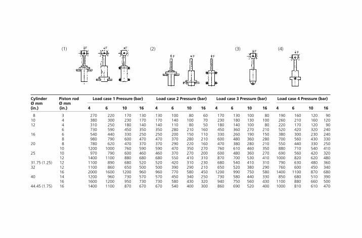
Cylinder Piston rod Load case 1 Pressure (bar) Load case 2 Pressure (bar) Load case 3 Pressure (bar) Load case 4 Pressure (bar)Ø mm Ø mm (in.) (in.) 4 6 10 16 4 6 10 16 4 6 10 16 4 6 10 16
8 3 270 220 170 130 130 100 80 60 170 130 100 80 190 160 120 9010 4 380 300 230 170 170 140 100 70 230 180 130 100 260 210 160 12012 4 310 250 180 140 140 110 80 50 180 140 100 80 220 170 120 90
6 730 590 450 350 350 280 210 160 450 360 270 210 520 420 320 24016 6 540 440 330 250 250 200 150 110 330 260 190 150 380 300 230 240
8 980 790 600 470 470 370 280 210 600 480 360 280 700 560 430 33020 8 780 620 470 370 370 290 220 160 470 380 280 210 550 440 330 250
10 1200 1000 760 590 590 470 350 270 760 610 460 350 880 710 540 41025 10 970 790 600 460 460 370 270 200 600 480 360 270 690 560 420 320
12 1400 1100 880 680 680 550 410 310 870 700 530 410 1000 820 620 48031.75 (1.25) 12 1100 890 680 520 520 420 310 230 680 540 410 310 790 630 480 36032 12 1100 860 650 500 500 390 290 210 650 520 380 290 760 600 450 340
16 2000 1600 1200 960 960 770 580 450 1200 990 750 580 1400 1100 870 68040 14 1200 960 730 570 570 450 340 250 730 580 440 330 850 680 510 390
16 1600 1200 950 730 730 580 430 320 940 750 560 430 1100 880 660 50044.45 (1.75) 16 1400 1100 870 670 670 540 400 300 860 690 520 400 1000 810 610 470
F(4)
F(3)
F F F
(2)F F F(1)

50 20 2000 1600 1200 930 930 740 550 420 1200 960 720 550 1400 1100 840 64050.8(2) 20 1900 1600 1200 930 930 740 550 420 1200 960 720 550 1400 1100 840 64063 20 1500 1200 930 720 720 570 420 310 930 740 550 420 1100 860 650 49063.5 (2.5) 25 2400 2000 1500 1200 1200 930 700 530 1500 1200 900 690 1700 1400 1100 81076.2 (3) 25 2000 1600 1200 950 950 760 560 420 1200 980 740 560 1400 1100 860 66080 25 1900 1500 1100 880 880 700 510 380 1100 910 680 510 1300 1100 800 600100 25 1500 1200 880 670 670 520 380 270 880 690 510 370 1000 820 600 450101.6 (4) 32 2400 2000 1500 1100 1100 910 670 500 1500 1200 890 670 1700 1400 1000 790125 32 2000 1600 1200 910 910 710 520 380 1200 940 690 520 1400 1100 820 620127 (5) 38.1 (1.5) 2800 2200 1700 1300 1300 1000 760 570 1700 1300 1000 760 2000 1600 1200 900152.4 (6) 38.1 (1.5) 2300 1800 1400 1100 1100 830 610 440 1400 1100 810 600 1600 1300 950 720160 40 2400 1900 1500 1100 1100 880 640 480 1400 1200 860 640 1700 1400 1000 760200 40 1900 1500 1100 860 860 670 480 350 1100 890 650 480 1300 1000 770 580203.2 (8) 44.45 (1.75) 2300 1900 1400 1100 1100 840 610 440 1400 1100 810 600 1600 1300 960 720250 50 2400 1900 1400 1100 1100 850 620 440 1400 1100 830 610 1700 1300 980 730254 (10) 57.15 (2.25) 3100 2500 1900 1400 1400 1100 840 620 1900 1500 1100 830 2200 1700 1300 990304.8 (12) 57.15 (2.25) 2500 2000 1500 1200 1200 920 660 480 1500 1200 890 660 1800 1400 1100 790320 63 3000 2400 1800 1400 1400 1100 780 570 1800 1400 1000 780 2100 1700 1200 930355.6 (14) 57.15 (2.25) 2100 1700 1300 970 970 760 540 380 1300 1000 730 540 1500 1200 870 650

Valve flowThere are a variety of standards and methods for the measurement and display of valveflow performance. These can give rise to confusion and difficulty when comparing thepublished performance of different valves. The table below provides conversion factors asa guide to expressing valve performance in different units.
Flow factor conversion table
Factors Flow* Orifice Size
Cv Kv C m3/h l/min A S†Cv 1 0.869 4.08 59.1 985 16.3 21.5Kv 1.15 1 4.69 67.9 1132 18.7 24.7C 0.245 0.213 1 14.5 241 4.11 5.27M3/h 0.017 0.015 0.069 1 16.67 0.276 0.364l/min 0.001 0.0088 0.0041 0.06 1 0.016 0.022A 0.061 0.053 0.243 3.62 60.4 1 1.31S 0.046 0.040 0.189 2.75 45.8 0.761 1
* Flow parameters are 6 bar inlet and 5 bar outlet at 20°C, 1013 mbar and 65% humidity.† ‘Cv’ is specified by ANSI/NFPA.Source: IMI Norgen Ltd.
How to useSelect the unit of measurement that is known in the left hand column and multiply by thefactor given in the column of the required unit of measurement:
‘Cv’ is specified by ANSI/NFPA.‘Kv’ used in Germany and based on water flow.‘C’ sonic conductance in dm3/s/bar specified by ISO 6358.‘A’ effective area in mm2 specified by ISO 6358.‘S’ effective area in mm2 according to the Japanese standard JIS B 8375.
A further measurement is the NW value. This gives the equivalent diameter in mm2 of thesmallest path through a valve. This is non-comparable and not in the table.
LubricantsWhen to lubricate, via an oil-fog or micro-fog lubricator, is generally explained in this cat-alogue. However, the oil recommended is very much dependant on the local conditionsand not least availability of various brands and labels.
In each country Norgren can recommend equivalent products, based on the informationfrom the suppliers.
5.6.20 Guideline documents
546 Mechanical Engineer’s Pocket Book
BFPA/P3 1995 Guidelines for the SafeApplication of Hydraulic andPneumatic Fluid PowerEquipment
BFPA/P4 1986 Guidelines for the Design ofQuieter Hydraulic FluidPower Systems (Third Edition)
BFPA/P5 1999 Guidelines to ContaminationControl in Hydraulic FluidPower Systems
BFPA/P7 2004 Guidelines to the Design,Installation andCommissioning of PipedSystems Part 1 – Hydraulics
BFPA/P9 1992 Guidelines for the Flushingof Hydraulic Systems
BFPA/P12 1995 Hydraulic Fluids Mineral OilData Sheets
BFPA/P13 1996 Fire-Resistant HydraulicFluids Data Sheets
continued
H6508-Ch05.6.qxd 9/12/05 4:48 PM Page 546

Power Transmission 547
BFPA/P22 2003 Guidelines on Selection ofIndustrial O-Rings (Metric &Inch)
BFPA/P27 1993 Guidelines onUnderstanding the ElectricalCharacteristics of Solenoidsfor Fluid Power ControlValves & their Application inPotentially ExplosiveAtmospheres
BFP/P28 1994 Guidelines for Errors andAccuracy of Measurementsin the Testing of Hydraulic &Pneumatic Fluid PowerComponents
BFPA/P29 1987 General conditions for thePreparation of Terms andConditions of Sale of UKFluid Power EquipmentManufacturers and Suppliers
BFPA/P41 1995 Guidelines to Hydraulic FluidPower Control Components
BFPA/P44 1995 Index of BS/ISO StandardsRelating to Fluid Power
BFPA/P47 2004 Guidelines to the Use ofHydraulic Fluid Power Hoseand Hose Assemblies
BFPA/P48 1998 Guidelines to theCleanliness of HydraulicFluid Power Components
BFPA/P49 1995 Guidelines to Electro-hydraulic Control Systems
BFPA/P52 1997 Guidelines to the Pluggingof Hydraulic Manifolds andComponents
BFPA/P53 2002 Fluid Power at the Forefront
BFPA/P54 2003 Guidelines to the PressureSystem Safety Regulations2000 and their Applicationto Gas-loaded Accumulators
BFPA/P55 1993 Guidelines for theComparison of ParticleCounters and CountingSystems for the Assessmentof Solid Particles in Liquid
BFPA/P56 2004 BFPA Fluid Power, Engineer’sData Booklet
BFPA/P57 1993 Guidelines to the Use ofEcologically AcceptableHydraulic Fluids in HydraulicFluid Power Systems
BFPA/P58 2003 The Making of Fluid PowerStandards
BFPA/P59 1993 Proceedings of the 1993BFPA Leak-Free HydraulicsSeminar
BFPA/P60 1994 Leak-Free for HydraulicConnections
BFPA/P61 1998 A Guide to the Use of CEMark
BFPA/P65 1995 VDMA 24 568 & 24 569Rapidly BiologicallyDegradable Hydraulic FluidsMinimum TechnicalRequirements & Conversionfrom Fluids based onMineral Oils
BFPA/P66 1995 BFPA Survey on EcologicallyAcceptable Hydraulic Fluids
BFPA/P67 1996 Ecologically AcceptableHydraulic Fluids Data Sheets
BFPA/P68 1995 Machinery DirectiveManufacturers Declarations
BFPA/P83 2003 The World of Fluid Power2003 CD Rom (Edition 3)
BFPA/P95 2003 Principles of HydraulicSystem Design
BFPA/P100 2003 Guidelines for the Proof &Burst Pressure Testing ofFluid Power Components
BFPDA/D2 1994 Technical Guidelines forDistributors of HydraulicFluid Power Equipment
Available from British fluid power associationSource: Page 27 BFPA hand book.
For further information relating to fluid power transmission equipment the reader isreferred to the companies and associations listed in Appendix 3.
Section 5.6.20 (continued )
H6508-Ch05.6.qxd 9/12/05 4:48 PM Page 547
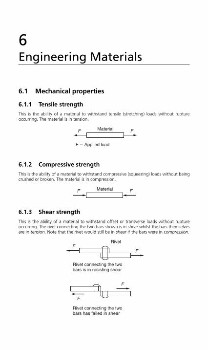
6Engineering Materials
6.1 Mechanical properties
6.1.1 Tensile strength
This is the ability of a material to withstand tensile (stretching) loads without ruptureoccurring. The material is in tension.
6.1.2 Compressive strength
This is the ability of a material to withstand compressive (squeezing) loads without beingcrushed or broken. The material is in compression.
6.1.3 Shear strength
This is the ability of a material to withstand offset or transverse loads without ruptureoccurring. The rivet connecting the two bars shown is in shear whilst the bars themselvesare in tension. Note that the rivet would still be in shear if the bars were in compression.
FRivet
F
F
Rivet connecting the twobars is in resisting shear
Rivet connecting the twobars has failed in shear
F
F Material F
F Material F
F � Applied load
H6508-Ch06.1.qxd 9/12/05 4:52 PM Page 548
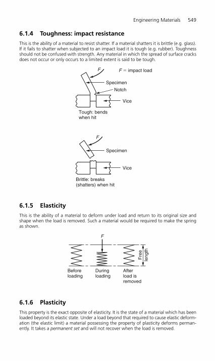
Engineering Materials 549
6.1.4 Toughness: impact resistance
This is the ability of a material to resist shatter. If a material shatters it is brittle (e.g. glass).If it fails to shatter when subjected to an impact load it is tough (e.g. rubber). Toughnessshould not be confused with strength. Any material in which the spread of surface cracksdoes not occur or only occurs to a limited extent is said to be tough.
6.1.5 Elasticity
This is the ability of a material to deform under load and return to its original size andshape when the load is removed. Such a material would be required to make the springas shown.
6.1.6 Plasticity
This property is the exact opposite of elasticity. It is the state of a material which has beenloaded beyond its elastic state. Under a load beyond that required to cause elastic deform-ation (the elastic limit) a material possessing the property of plasticity deforms perman-ently. It takes a permanent set and will not recover when the load is removed.
Beforeloading
Duringloading
Afterload isremoved
Fre
ele
ngth
F
Vice
Specimen
Notch
Tough: bendswhen hit
F F � impact load
Vice
Specimen
Brittle: breaks(shatters) when hit
F
H6508-Ch06.1.qxd 9/12/05 4:52 PM Page 549
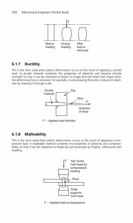
6.1.7 Ductility
This is the term used when plastic deformation occurs as the result of applying a tensileload. A ductile material combines the properties of plasticity and tenacity (tensilestrength) so that it can be stretched or drawn to shape and will retain that shape whenthe deforming force is removed. For example, in wire drawing the wire is reduced in diam-eter by drawing it through a die.
6.1.8 Malleability
This is the term used when plastic deformation occurs as the result of applying a com-pressive load. A malleable material combines the properties of plasticity and compress-ibility, so that it can be squeezed to shape by such processes as forging, rolling and rivetheading.
F � Applied load (compressive)
Rivet
F ‘Set’ formsrivet head bycompressiveloading
‘Dolly’supportsrivet head
Die
Wire
Ductilematerial
Directionof draw
F � Applied load (tensile)
F
Beforeloading
Duringloading
Afterload isremoved
F
550 Mechanical Engineer’s Pocket Book
H6508-Ch06.1.qxd 9/12/05 4:52 PM Page 550

Engineering Materials 551
6.1.9 Hardness
This is the ability of a material to withstand scratching (abrasion) or indentation byanother hard body. It is an indication of the wear resistance of a material.
Processes which increase the hardness of materials also increase their tensile strength. Atthe same time the toughness of the material is reduced as it becomes more brittle.
Hardenability must not be confused with hardness. Hardenability is the ability of a metalto respond to the heat treatment process of quench hardening. To harden it, the hotmetal must be chilled at a rate in excess of its critical cooling rate. Since any material coolsmore quickly at the surface than at the centre there is a limit to the size of bar which can cool quickly enough at its centre to achieve uniform hardness throughout. This is theruling section for the material. The greater its hardenability the greater will be its rulingsection.
6.1.10 Tensile test
The tensile test is widely used for determining the strength and ductility of a material. Thetest involves loading a standard specimen axially as shown. The load is increased at a con-stant rate mechanically or hydraulically. The specimen increases in length until it finallyfractures. During the test the specimen is gripped at each end to ensure simple uniaxialloading and freedom of bending. The extension is measured from the gauge length. Themid-portion of the specimen is reduced in diameter as shown to ensure fracture occurswithin the gauge length.
Same prescribed load
Soft material: greaterindentation for same load
Prescribed load
Hard material:little indentation
Hardenedball indenter
Materialbeing tested
H6508-Ch06.1.qxd 9/12/05 4:52 PM Page 551
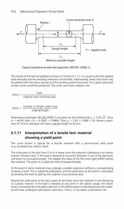
The results of the test are plotted as shown in Section 6.1.11; it is usual to plot the appliedload vertically and the resulting extension horizontally. Alternatively, stress and strain maybe plotted with the stress vertical and the resulting strain horizontal. For a given specimensimilar curves would be produced. The stress and strain relations are:
Proportional specimens (BS EN 10002-1) are given by the relationship L0 � 5.65�––A . Since
A � �d2/4, then �––A � d�––––
(�)/2 � 0.886d. Thus L0 � 5.65 � 0.886 � 5d. Hence a speci-men of 10-mm diameter will have a gauge length of 50 mm.
6.1.11 Interpretation of a tensile test: material showing a yield point
The curve shown is typical for a ductile material with a pronounced yield point (e.g. annealed low carbon steel).
The initial part of the plot from O to A is linear since the material is behaving in an elasticmanner (Hooke’s law). If the load is released at any point between O and A the specimenwill return to its original length. The steeper the slope of OA the more rigid (stiffer) will bethe material. The point A is called the limit of proportionality.
At the point A some materials may undergo a sudden extension without a correspondingincrease in load. This is called the yield point, and the yield stress at this point is calculatedby dividing the load at yield by the original cross-sectional area.
Beyond the yield point A the plot ceases to be linear since the material is now behavingin a plastic manner. If the load is released at any point in the plastic range, the elasticstrain is recovered but the plastic element of the deformation is maintained and the mater-ial will have undergone permanent extension. That is, it has taken a permanent set.
Strainincrease in length under load
origina�
ll length
Stressload
original cross-sectional area�
Radius rCross-sectional area A
Gauge length
Minimum parallel length
Typical cylindrical tensile test specimen (BS EN 10002-1)
F � Applied load
FFfd
L0
Lc
552 Mechanical Engineer’s Pocket Book
H6508-Ch06.1.qxd 9/12/05 4:52 PM Page 552
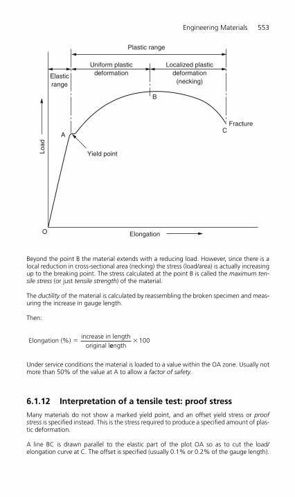
Beyond the point B the material extends with a reducing load. However, since there is alocal reduction in cross-sectional area (necking) the stress (load/area) is actually increasingup to the breaking point. The stress calculated at the point B is called the maximum ten-sile stress (or just tensile strength) of the material.
The ductility of the material is calculated by reassembling the broken specimen and meas-uring the increase in gauge length.
Then:
Under service conditions the material is loaded to a value within the OA zone. Usually notmore than 50% of the value at A to allow a factor of safety.
6.1.12 Interpretation of a tensile test: proof stress
Many materials do not show a marked yield point, and an offset yield stress or proofstress is specified instead. This is the stress required to produce a specified amount of plas-tic deformation.
A line BC is drawn parallel to the elastic part of the plot OA so as to cut the load/elongation curve at C. The offset is specified (usually 0.1% or 0.2% of the gauge length).
Elongation (%)increase in length
original l�
eength100�
Elongation
Yield pointLoad
Fracture
Localized plasticdeformation
(necking)
Uniform plasticdeformationElastic
range
Plastic range
A
B
C
O
Engineering Materials 553
H6508-Ch06.1.qxd 9/12/05 4:52 PM Page 553
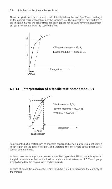
The offset yield stress (proof stress) is calculated by taking the load F1 at C and dividing itby the original cross-sectional area of the specimen A0. The material will have fulfilled itsspecification if, after the proof stress has been applied for 15 s and removed, its perman-ent set is not greater than the specified offset.
6.1.13 Interpretation of a tensile test: secant modulus
Some highly ductile metals such as annealed copper and certain polymers do not show alinear region on the tensile test plot, and therefore the offset yield stress (proof stress)cannot be determined.
In these cases an appropriate extension is specified (typically 0.5% of gauge length) andthe yield stress is specified as the load to produce a total extension of 0.5% of gaugelength divided by the original cross-section area A0.
In place of an elastic modulus the secant modulus is used to determine the elasticity ofthe material.
Elongation
Load
A
BO
Yield stress � F1/A0
Secant modulus � (L0/A0)S
Where S � OA/OB
0.5% ofgauge length
F1
Slo
pe �
S
Elongation
Load
A
BO
C
Offset yield stress � F1/A0
Elastic modulus � slope of BC
Offset
F1
554 Mechanical Engineer’s Pocket Book
H6508-Ch06.1.qxd 9/12/05 4:52 PM Page 554

Engineering Materials 555
6.1.14 Impact testing for toughness: Izod test
In the Izod impact test a 10-mm square notched test piece is used. It is supported as acantilever in the vice of the testing machine and struck with a kinetic energy of 162.72 Jat a velocity of 3.8 m/s. The energy absorbed in deforming or breaking the test piece is itstoughness factor. BS 131 (metals), BS 2782-350 (plastics).
6.1.15 Impact testing for toughness: Charpy test
R 1.0
R 1.0
R 1.0
2.0
u = 22½°u u
V-notch
3 or 5
2, 3 or 5
2.0
Key holenotch
U-notch
Standard Charpy notches
Dimensionsin mm
Section throughtest piece (at notch)
Test pieceStriker
2.0–2.5
R 0.25
R 1.0–1.5
1830°22½°
22½°
78–80°
810
10
Vice
Tes
t pie
ce
Dimensions in mm
5°
10°22½°
228
70
22
22½°Striker
Root radius0.25
Detailsof notch
108
10
Section of testpiece at notch
H6508-Ch06.1.qxd 9/12/05 4:52 PM Page 555

556 Mechanical Engineer’s Pocket Book
In the Charpy impact test a 10-mm square specimen is supported as a beam and struckwith a kinetic energy of 298.3 J at a velocity of 5 m/s. The energy absorbed in bending or breaking the test piece is its toughness factor. BS EN 10045 (metals), BS 131-6 and BS 131-7 (metals), BS 2782-359 (plastics).
6.1.16 Interpretation of impact test results
Brittle metals There is a clean break with little reduction in cross-sectional area. Thefractured surfaces show a granular structure.
Ductile metals The fracture is rough and fibrous. In very ductile metals the fracturemay not be complete: the test piece bends over and only shows slight tearing from thenotch. There will also be some reduction in cross-sectional area at the point of fracture orbending.
Brittle polymers There is a clean break showing smooth, glassy fractured surfaceswith some splintering.
Ductile polymers There is no distinctive appearance to the fracture if one occurs at all.There will be a considerable reduction in cross-sectional area and some tearing at the notch.
Crack spread Since the Izod and Charpy tests both use notched test pieces, usefulinformation can be obtained regarding the resistance of a material to the spread of acrack. Such a crack may originate from a point of stress concentration and indicates theneed to avoid sharp corners, undercuts, sudden changes in sections and machining marks.
6.1.17 Brinell hardness test
In this test a hardened steel ball is pressed into the surface of the test piece using a pre-scribed load. The combination of load and ball diameter have to be related to the mater-ial under test to avoid errors of distortion. The test piece hardness should be limited toHB � 500, otherwise the ball indenter will tend to flatten and introduce errors (BS 240).
where:P � load (kg)D � diameter of indenter (mm)k � 30 for ferrous metals
� 10 for copper and copper alloys
PD
k2
�
Load P
Test piece
fD
fd
Ballindenter
H6508-Ch06.1.qxd 9/12/05 4:52 PM Page 556

Engineering Materials 557
� 5 for aluminium and aluminium alloys� 1 for lead, tin, white-bearing metals
6.1.18 Vickers hardness test
In this test a diamond indenter is used in the form of a square-based pyramid with anangle of 136° between facets. Since diamond has a hardness of 6000 HB, this test can beused for testing very hard materials. Only one size of indenter is used and the load is var-ied. Standard loads are 5, 10, 20, 30, 50 and 100 kg. It is necessary to state the test loadwhen specifying a Vickers hardness number (e.g. HD(50) � 200).
where:P � load (kg)D � diagonal length of indentation (average)
BS 427, BS EN 23878 (hard metals), BS 411-6 (metallic coatings) BS 6479 (case-hardenedsteels), BS 6481 (flame and induction hardened steels), DD ENV 843-4 (monolithic ceramics).
6.1.19 Rockwell hardness test
This test uses either a hard steel ball for softer materials or a 120° diamond cone indenter for harder materials. The test compares the differences in depth of penetrationbetween a minor initial load (98 N) and a major additional load. The result of the test isread directly from the machine scale.
Hardness value 1.844D 2H
P
D�
D1
D2
D �D1 � D2
2
Appearance of indentation
�� �
P
D D D dp( /2)[ ( ) ]2 2
Hardness number ( )load
spherical area ofBH �iindentation
H6508-Ch06.1.qxd 9/12/05 4:52 PM Page 557
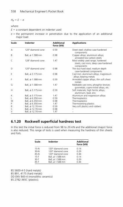
558 Mechanical Engineer’s Pocket Book
HR � E � e
where:E � a constant dependent on indenter used
e � the permanent increase in penetration due to the application of an additional major load
Scale Indenter Additional Applicationsforce (kN)
A 120° diamond cone 0.59 Sheet steel; shallow case-hardened components
B Ball, � 1.588 mm 0.98 Copper alloys; aluminium alloys; annealed low-carbon steels
C 128° diamond cone 1.47 Most widely used range; hardened steels; cast irons; deep case-hardened components
D 120° diamond cone 0.98 Thin but hard steel; medium depth case-hardened components
E Ball, � 3.175 mm 0.98 Cast iron; aluminium alloys, magnesium alloys; bearing metals
F Ball, � 1.588 mm 0.59 Annealed copper alloys; thin soft sheet metals
G Ball, � 1.588 mm 1.47 Malleable cast irons; phosphor bronze; gunmetals; cupro-nickel alloys, etc.
H Ball, � 3.175 mm 0.59 Soft materials; high ferritic alloys; aluminium; lead; zinc
K Ball, � 3.175 mm 1.47 Aluminium and magnesium alloysL Ball, � 6.350 mm 0.59 ThermoplasticsM Ball, � 6.350 mm 0.98 ThermoplasticsP Ball, � 6.350 mm 1.47 Thermosetting plasticsR Ball, � 12.70 mm 0.59 Very soft plastics and rubbersS Ball, � 12.70 mm 0.98 –V Ball, � 12.70 mm 1.47 –
6.1.20 Rockwell superficial hardness test
In this test the initial force is reduced from 98 to 29.4 N and the additional (major) forceis also reduced. This range of tests is used when measuring the hardness of thin sheetsand foils.
BS 5600-4-5 (hard metals)BS 891, 4175 (hard metals)DD ENV 843-4 (monolithic ceramics)BS 2782-365C (plastics).
Scale Indenter Additional force (kN)
15-N 120° diamond cone 0.1430-N 120° diamond cone 0.2945-N 120° diamond cone 0.4415-T Ball, � 1.588 mm 0.1430-T Ball, � 1.588 mm 0.2945-T Ball, � 1.588 mm 0.44
H6508-Ch06.1.qxd 9/12/05 4:52 PM Page 558
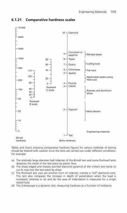
Engineering Materials 559
6.1.21 Comparative hardness scales
Tables and charts showing comparative hardness figures for various methods of testingshould be treated with caution since the tests are carried out under different conditions.For example:
(a) The relatively large diameter ball indenter of the Brinell test and some Rockwell testsdisplaces the metal of the test piece by plastic flow.
(b) The sharp edged and sharply pointed diamond pyramid of the Vickers test tends tocut its way into the test piece by shear.
(c) The Rockwell test uses yet another form of indenter, namely a 120° diamond cone.This test also compares the increase in depth of penetration when the load isincreased, whereas in (a) and (b) the area of indentation is measured for a singlestated load.
(d) The Scleroscope is a dynamic test, measuring hardness as a function of resilience.
10 000
5000
2000
1000
500
200
100
100
110
50
20
20
20
0
0
40
40
60
60
80
80
10
10
5
9
8
7
6
5
43
2
1Brinellhardness
RockwellB scale
RockwellC scale
Diamond
Corundum orsapphire
Topaz
Quartz
Orthoclase
Apatite
FluoriteCalcite
Gypsum
Talc
Mohs hardness
Nitrided steels
Cutting tools
File hard
Machinable steels (usingHSS tool)
Brasses and aluminiumalloys
Most plastics
Engineering materials
H6508-Ch06.1.qxd 9/12/05 4:52 PM Page 559

560 Mechanical Engineer’s Pocket Book
6.2 Ferrous metals and alloys
6.2.1 Ferrous metals: plain carbon steels
Ferrous metals are based on the metallic element iron (Latin ferrum � iron). The iron isassociated with carbon, either as a solid solution or as the chemical compound iron car-bide (cementite). In the case of cast irons, some amount of carbon may be uncombined(free) in the form of flake graphite. In addition to carbon, other elements may also bepresent. These may be impurities such as sulphur and phosphorus which weaken themetal and are kept to a minimum. Alloying elements are added to enhance the perform-ance of the metal (e.g. chromium and nickel).
Plain carbon steels consist mainly of iron and carbon, and are the simplest of the ferrousmetals. Some manganese will also be present to neutralize the deleterious effects of thesulphur and to enhance the grain structure. It is not present in sufficient quantity to beconsidered as an alloying element.
The amount of carbon present affects the properties of the steel as shown in 6.2.3. Themaximum amount of carbon which can remain combined with the iron at all tempera-tures is 1.7%. In practice an upper limit of 1.2–1.4% is set to ensure a margin of safety.A steel, by definition, must contain no free carbon.
Low-carbon steelsThese have a carbon content 0.1–0.3% plus impurities, plus some manganese to neutralizethe effect of any sulphur content left over from the extraction process. Such steels cannotbe directly hardened by heat treatment, but they can be readily carburized and case hard-ened. The lower-carbon steels in this category are used for steel sheets for pressing out suchcomponents as motorcar body panels as they have a high ductility. The lower-carbon steelsin this category are also made into drawn wire rod and tube. The higher-carbon steels in thiscategory are stiffer and less ductile, and are used for general workshop bars, plates and gird-ers. Low-carbon steels are substantially stronger than wrought iron which is no longer considered to be a structural material.
Medium-carbon steels
(a) Carbon content 0.3–0.5%: Such steels can be toughened by heat treatment (heatingto red heat and quenching – rapid cooling – in water). They are used for crankshaftand axle forgings where cost is important and the service requirements do not war-rant stronger but more expensive alloy steels.
(b) Carbon content 0.5–0.8%: These are used for vehicle leaf springs and garden tools.Such steels can be quench hardened by heat treatment as above.
High-carbon steelsAll high carbon steels can be hardened to a high degree of hardness by heating to a dullred heat and quenching. The hardness and application depend on the carbon content,the rate of cooling from the hardening temperature and the degree of tempering afterhardening:
(a) Carbon content 0.8–1.0%; used for coil springs and wood chisels.(b) Carbon content 1.0–1.2%; used for files, drills, taps and dies.(c) Carbon content 1.2–1.4%; used for fine-edge tools (knives, etc.).
H6508-Ch06.2.qxd 9/21/05 10:04 AM Page 560

6.2.2 Effect of carbon content on the composition, properties and uses of plain carbon steels
1000
800
600
400
200
0
TinplateScrewsR.S.J.
Motorcar bodiesRivetsNailsWire
Conn. rodsAxlesShaftsGears Screw
driversRails
Cold chiselsShear bladesSome hand tools
DiesTapsDrills
ReamersBroachesKnivesFiles
RazorsSaws
70
60
50
40
30
20
10
0
Cha
rpy
impa
ct v
alue
(J)
30
20
10
0 0.2 0.4 0.6 0.8 1.0 1.2 1.4
150
200
250
300
35050
40
Carbon (%)
Brin
ell h
ardn
ess
Elo
ngat
ion
(%)
Ten
sile
str
engt
h (N
/mm
2 )
Elongation %
Tensile st
rength
Brinell h
ardness
Charpy impact
6.2.3 Ferrous metals: alloying elements
Alloy steels are carbon steels containing less than 1% carbon but to which other metalshave been added in sufficient quantities to alter the properties of the steel significantly.The more important alloying elements are as follows:
Aluminium Up to 1% aluminium in alloy steels enables them to be given a hard, wear-resistant skin by the process of nitriding.
Chromium The presence of small amounts of chromium stabilizes the formation ofhard carbides. This improves the response of the steel to heat treatment. The presence oflarge amounts of chromium improves the corrosion resistance and heat resistance of thesteel (e.g. stainless steel). Unfortunately, the presence of chromium in a steel leads tograin growth (see nickel ).
Engineering Materials 561
H6508-Ch06.2.qxd 9/21/05 10:04 AM Page 561

Cobalt Cobalt induces sluggishness into the response of a steel to heat treatment. Intool steels it allows them to operate at high-level temperatures without softening. It is animportant alloying element in some high-speed steels.
Copper Up to 0.5% copper improves the corrosion resistance of alloy steels.
Lead The presence of up to 0.2% lead improves the machinability of steels, but at theexpense of reduced strength and ductility.
Manganese This alloying element is always present in steels up to a maximum of 1.5%to neutralize the deleterious effects of impurities carried over from the extraction process.It also promotes the formation of stable carbides in quench-hardened steels. In largerquantities (up to 12.5%) manganese improves the wear resistance of steels by spontan-eously forming a hard skin when subject to abrasion (self-hardening steels).
Molybdenum This alloying element raises the high-temperature creep resistance ofsteels; stabilizes their carbides; improves the high-temperature performance of cutting toolmaterials; and reduces the susceptibility of nickel–chrome steels to ‘temper brittleness’.
Nickel The presence of nickel in alloy steels results in increased strength and grainrefinement. It also improves the corrosion resistance of the steel. Unfortunately it tends tosoften the steel by graphitizing any carbides present. Since nickel and chromium haveopposite properties they are frequently combined together (nickel–chrome steels). Theiradvantages are complementary, whilst their undesirable effects are cancelled out.
Phosphorus This is a residual element from the extraction process. It causes weaknessin the steel, and usually care is taken to reduce its presence to below 0.05%. Nevertheless,it can improve machinability by acting as an internal lubricant. In larger quantities it alsoimproves the fluidity of cast steels and cast irons.
Silicon The presence of up to 0.3% silicon improves the fluidity of casting steels andcast irons without the weakening effects of phosphorus. Up to 1% silicon improves theheat resistance of steels. Unfortunately, like nickel, it is a powerful graphitizer and is neveradded in large quantities to high-carbon steels. It is used to enhance the magnetic prop-erties of ‘soft’ magnetic materials as used for transformer laminations and the stampingsfor electric motor stators and rotors.
Sulphur This is also a residual element from the extraction process. Its presence greatlyweakens steel, and every effort is made to refine it out; in addition, manganese is alwayspresent in steels to nullify the effects of any residual sulphur. Nevertheless, sulphur issometimes deliberately added to low-carbon steels to improve their machinability wherea reduction in component strength can be tolerated (sulphurized free-cutting steels).
Tungsten The presence of tungsten in alloy steels promotes the formation of very hardcarbides and, like cobalt, induces sluggishness into the response of the steel to heat treat-ment. This enables tungsten steels (high-speed steels) to retain their hardness at hightemperatures. Tungsten alloys form the bases of high-duty tool and die steels.
Vanadium This element enhances the effects of the other alloying elements presentand has many and varied effects on alloy steels:
(a) Its presence promotes the formation of hard carbides.(b) It stabilizes the martensite in quench-hardened steels and thus improves hardenabil-
ity and increases the limiting ruling section of the steel.(c) It reduces grain growths during heat treatment and hot-working processes.(d) It enhances the ‘hot hardness’ of tool steels and die steels.(e) It improves the fatigue resistance of steels.
562 Mechanical Engineer’s Pocket Book
H6508-Ch06.2.qxd 9/21/05 10:04 AM Page 562

Engineering Materials 563
6.2.4 British standards relating to ferrous metals
Although BS 970 is now obsolescent, it is still widely used but should not be quoted whenspecifying wrought steels for new designs and products. It has now been superceded bythe BS EN 10 000 series of specifications which are English language versions and com-patible with the Continental ISO specifications.
One advantage of BS 970: 1991 is that it changed the random numbering system of theearlier version and designates the steels by an alphanumeric code that indicates the actualcomposition of the material in a logical manner. The designation code of each steel is builtup as follows:
(a) The first three symbols are a number code indicating the type of steel:000 to 199 are carbon and manganese steels. The numbers represent the manganesecontent � 100.200 to 240 are free-cutting steels. The second and third numbers indicate the sulphurcontent � 100.250 are silicon manganese valve steels.300 to 499 are stainless and heat-resisting steels.500 to 999 are alloy steels.
(b) The fourth symbol is a letter code:A The steel is supplied to a chemical composition determined by chemical analysis
of a batch sample.H The steel is supplied to a hardenability specification.M The steel is supplied to a mechanical property specification.S The material is a stainless steel.
(c) The fifth and sixth symbol comprise a number code indicating the actual carbon content � 100
The following are examples of the BS 970: 1991 six-figure code:070M20 A plain carbon steel with a composition of 0.7% manganese and 0.2%
carbon. The M indicates that the steel has a prescribed mechanical propertyspecification.
230M07 A low-carbon, free-cutting steel with a sulphur content of 0.3% and a carboncontent of 0.7%.
080A15 A plain carbon steel with a manganese content of 0.8% and a carbon contentof 0.15%. The A indicates that the steel must meet a prescribed chemical com-position specification.
Unfortunately for alloy steels coded between 500 and 999 the logicality of the first three digits breaks down. In addition to the six-figure grading code, a condition code isapplied. The code letter indicates the tensile strength range for a given steel after heattreatment. The final factor to be considered in the coding of wrought steels is the limiting ruling section. As explained in Section 6.1.9 this is the maximum diameter of barof a given composition which, after heat treatment, will attain the specified mechanicalproperties.
For example, a plain carbon steel of composition 070M55(R) containing 0.7% manganeseand 0.55% carbon can attain condition (R) after heat treatment providing it is not greaterthan 100-mm diameter, however if it is to attain condition (S) then its maximum diametermust not exceed 63 mm. In the first example the limiting ruling section is 100 mm and inthe second example the limiting ruling section is 63 mm in diameter. This letter/strengthrelationship code is listed in Table 6.1. The condition code is applied in brackets after thesix-symbol code as shown above.
In addition to the standard chemical symbols used to denote the composition of a metal(e.g. C � carbon, Mn � manganese, P � phosphorus, S � sulphur, etc.), the symbols
H6508-Ch06.2.qxd 9/21/05 10:04 AM Page 563

564 Mechanical Engineer’s Pocket Book
used in tables of mechanical properties are as follows:
Tensile propertiesRm Tensile strengthRe Yield strengthA Percentage elongation after fractureSo Original cross-sectional area of the gauge lengthRp02 0.2% proof stress (non-proportional elongation)Rp1.0 1.0% proof stress (non-proportional elongation)Rt0.5 0.5% proof stress (total elongation)Rt1.0 1.0% proof stress (total elongation)ReH Upper yield stress
Impact propertiesKCV Charpy V-notch impact value
HardnessHB Brinell hardnessHV Vickers hardnessHRC Rockwell hardness (C scale)
OtherLRS the limiting ruling section.
Note that the specifications for the chemical composition and mechanical properties forplain carbon and alloy steels are now being superceded by the BS EN 10000 series of stand-ards. For example:
● BS EN 10277-2 1999 deals with the composition and mechanical properties of plaincarbon bright steel products.
● BS EN 10277-3 deals with the composition and mechanical properties of free-cutting steels.● BS EN 10277-4 deals with the chemical composition and mechanical properties of
case-hardening steels.● BS EN 10277-5 deals with non-alloy and alloy steels suitable for quench hardening and
tempering.
The steels are now designated by a steel name and a steel number. For example a plaincarbon steel containing 0.13–0.18% carbon and 0.7–0.9% manganese would be desig-nated 080A15 in BS 970 it is now designated: steel name C15 and steel number1.0401 in BS EN 10277-2.
BS EN 10277 and related standards for steels are highly detailed and comprehensive, andit is not physically possible to reproduce them in this Pocket Book. These standards shouldbe consulted together with BS Guide Lines PD 970:2005 when selecting a suitable steelfor a new product design and manufacture. Some examples of typical steels and theirapplications are listed in Section 6.2.5 and some examples of typical tool and die steelsare listed in Section 6.2.6.
Table 6.1 Code letter/strength relationship
Condition Tensile strength (MPa) Condition Tensile strength (MPa)code letter
min. max.code letter
min. max.
P 550 700 V 1000 1150Q 620 770 W 1080 1240R 700 850 X 1150 1300S 770 930 Y 1240 1400T 850 1000 Z 1540 –U 930 1080
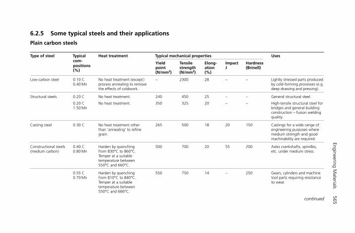
Engineering Materials
565
6.2.5 Some typical steels and their applications
Plain carbon steels
Type of steel Typical Heat treatment Typical mechanical properties Usescom- Yield Tensile Elong- Impact Hardness positions point strength ation J (Brinell)(%) (N/mm2) (N/mm2) (%)
Low-carbon steel 0.10 C No heat treatment (except ) – 2300 28 – – Lightly stressed parts produced 0.40 Mn process annealing to remove by cold-forming processes (e.g.
the effects of coldwork. deep drawing and pressing).
Structural steels 0.20 C No heat treatment. 240 450 25 – – General structural steel.
0.20 C No heat treatment. 350 325 20 – – High-tensile structural steel for 1.50 Mn bridges and general building
construction – fusion welding quality.
Casting steel 0.30 C No heat treatment other 265 500 18 20 150 Castings for a wide range of than ‘annealing’ to refine engineering purposes where grain. medium strength and good
machinability are required.
Constructional steels 0.40 C Harden by quenching 500 700 20 55 200 Axles crankshafts, spindles, (medium carbon) 0.80 Mn from 830°C to 860°C. etc. under medium stress.
Temper at a suitable temperature between 550°C and 660°C.
0.55 C Harden by quenching 550 750 14 – 250 Gears, cylinders and machine 0.70 Mn from 810°C to 840°C. tool parts requiring resistance
Temper at a suitable to wear.temperature between 550°C and 666°C.
continued
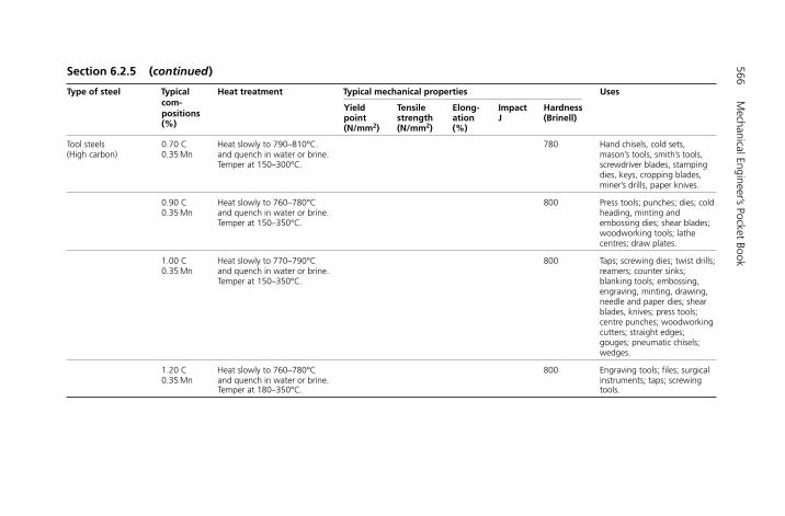
566M
echanical Engineer’s Pocket Book
Type of steel Typical Heat treatment Typical mechanical properties Usescom- Yield Tensile Elong- Impact Hardness positions point strength ation J (Brinell)(%) (N/mm2) (N/mm2) (%)
Tool steels 0.70 C Heat slowly to 790–810°C. 780 Hand chisels, cold sets, (High carbon) 0.35 Mn and quench in water or brine. mason’s tools, smith’s tools,
Temper at 150–300°C. screwdriver blades, stamping dies, keys, cropping blades, miner’s drills, paper knives.
0.90 C Heat slowly to 760–780°C 800 Press tools; punches; dies; cold 0.35 Mn and quench in water or brine. heading, minting and
Temper at 150–350°C. embossing dies; shear blades; woodworking tools; lathe centres; draw plates.
1.00 C Heat slowly to 770–790°C 800 Taps; screwing dies; twist drills; 0.35 Mn and quench in water or brine. reamers; counter sinks;
Temper at 150–350°C. blanking tools; embossing, engraving, minting, drawing, needle and paper dies; shear blades, knives; press tools; centre punches; woodworking cutters; straight edges; gouges; pneumatic chisels; wedges.
1.20 C Heat slowly to 760–780°C 800 Engraving tools; files; surgical 0.35 Mn and quench in water or brine. instruments; taps; screwing
Temper at 180–350°C. tools.
Section 6.2.5 (continued)
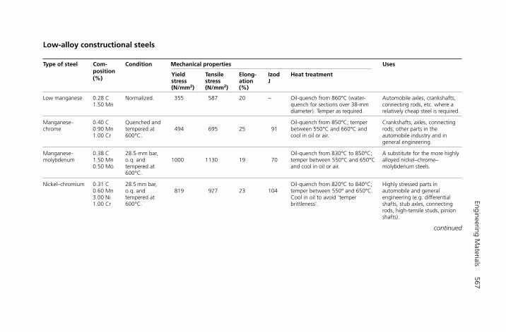
Engineering Materials
567
Low-alloy constructional steels
Type of steel Com- Condition Mechanical properties Usesposition Yield Tensile Elong- Izod Heat treatment(%) stress stress ation J
(N/mm2) (N/mm2) (%)
Low manganese 0.28 C Normalized. 355 587 20 – Oil-quench from 860°C (water- Automobile axles, crankshafts,1.50 Mn quench for sections over 38-mm connecting rods, etc. where a
diameter). Temper as required. relatively cheap steel is required.
Manganese– 0.40 C Quenched and Oil-quench from 850°C; temper Crankshafts, axles, connecting chrome 0.90 Mn tempered at 494 695 25 91 between 550°C and 660°C and rods; other parts in the
1.00 Cr 600°C. cool in oil or air. automobile industry and in general engineering.
Manganese– 0.38 C 28.5-mm bar, Oil-quench from 830°C to 850°C; A substitute for the more highly molybdenum 1.50 Mn o.q. and 1000 1130 19 70 temper between 550°C and 650°C alloyed nickel–chrome–
0.50 Mo tempered at and cool in oil or air. molybdenum steels.600°C.
Nickel–chromium 0.31 C 28.5 mm bar, Oil-quench from 820°C to 840°C; Highly stressed parts in 0.60 Mn o.q. and 819 927 23 104 temper between 550° and 650°C. automobile and general 3.00 Ni tempered at Cool in oil to avoid ‘temper engineering (e.g. differential 1.00 Cr 600°C. brittleness’. shafts, stub axles, connecting
rods, high-tensile studs, pinion shafts).
continued
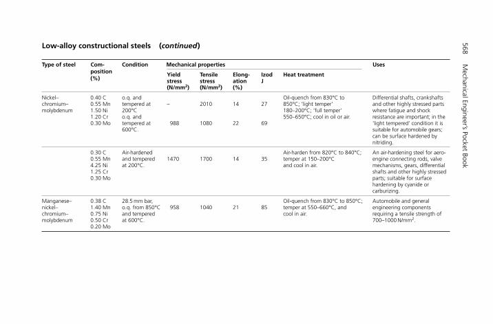
568M
echanical Engineer’s Pocket Book
Low-alloy constructional steels (continued)
Type of steel Com- Condition Mechanical properties Usesposition Yield Tensile Elong- Izod Heat treatment(%) stress stress ation J
(N/mm2) (N/mm2) (%)
Nickel– 0.40 C o.q. and Oil-quench from 830°C to Differential shafts, crankshafts chromium– 0.55 Mn tempered at – 2010 14 27 850°C; ‘light temper’ and other highly stressed parts molybdenum 1.50 Ni 200°C 180–200°C; ‘full temper’ where fatigue and shock
1.20 Cr o.q. and 550–650°C; cool in oil or air. resistance are important; in the 0.30 Mo tempered at 988 1080 22 69 ‘light tempered’ condition it is
600°C. suitable for automobile gears; can be surface hardened by nitriding.
0.30 C Air-hardened Air-harden from 820°C to 840°C; An air-hardening steel for aero-0.55 Mn and tempered 1470 1700 14 35 temper at 150–200°C engine connecting rods, valve 4.25 Ni at 200°C. and cool in air. mechanisms, gears, differential 1.25 Cr shafts and other highly stressed 0.30 Mo parts; suitable for surface
hardening by cyanide or carburizing.
Manganese– 0.38 C 28.5 mm bar, Oil-quench from 830°C to 850°C; Automobile and general nickel– 1.40 Mn o.q. from 850°C 958 1040 21 85 temper at 550–660°C, and engineering components chromium– 0.75 Ni and tempered cool in air. requiring a tensile strength of molybdenum 0.50 Cr at 600°C. 700–1000 N/mm2.
0.20 Mo
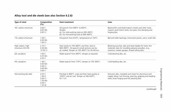
Engineering Materials
569
Alloy tool and die steels (see also Section 6.2.6)
Type of steel Composition Heat treatment Uses(%)
‘60’ carbon-chromium 0.60 C Oil-quench from 800°C to 850°C. Blacksmith’s and boilermaker’s chisels and other tools; 0.65 Mn Temper: mason’s and miner’s tools; vice jaws; hot stamping and 0.65 Cr (a) For cold-working tools at 200–300°C. forging dies.
(b) For hot-working tools at 400–600°C.
1% carbon-chromium 1.00 C Oil-quench from 810°C; temperature at 150°C. Ball and roller bearings; instrument pivots; cams; small rolls.0.45 Mn1.40 Cr
High carbon, high 2.10 C Heat slowly to 750–800°C and then raise to Blanking punches, dies and shear blades for hard, thin chromium (HCCR) 0.30 Mn 960–990°C. Oil-quench (small sections can be materials; dies for moulding abrasive powders, (e.g.
12.50 Cr air cooled). Temper at 150–400°C for 30–60 min. ceramics; master gauges; thread rolling dies).
1–4% vanadium 1.00 C Water-quench from 850°C; temper as required. Cold-drawing dies, etc.0.25 Mn0.20 V
4% vanadium 1.40 C Water-quench from 770°C; temper at 150–300°C. Cold-heading dies, etc.0.40 Mn0.40 Cr0.40 Mo3.60 V
Hot-working die steel 0.35 C Pre-heat to 800°C, soak and then heat quickly to Extrusion dies, mandrels and noses for aluminium and 1.00 Si 1020°C and air cool. Temper at 540–620°C copper alloys; hot forming, piercing, gripping and heading 5.00 Cr for 11⁄2 h. tools; brass forging and hot pressing dies.1.50 Mo0.40 V1.35 W
continued
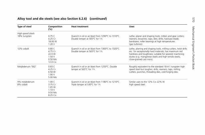
570M
echanical Engineer’s Pocket Book
Alloy tool and die steels (see also Section 6.2.6) (continued)
Type of steel Composition Heat treatment Uses(%)
High-speed steels18% tungsten 0.75 C Quench in oil or air blast from 1290°C to 1310°C. Lathe, planer and shaping tools; millers and gear cutters;
4.25 Cr Double temper at 565°C for 1 h. reamers; broaches; taps; dies; drills; hacksaw blade; 18.00 W bandsaws; roller bearings at high temperatures 1.20 V (gas turbines).
12% cobalt 0.80 C Quench in oil or air blast from 1300°C to 1320°C. Lathe, planing and shaping tools, milling cutters, twist drills 4.75 Cr Double temper at 565°C for 1 h. etc. for exceptionally hard materials; has maximum red 22.0 W hardness and toughness; suitable for severest machining 1.50 V duties (e.g. manganese steels and high tensile steels, 0.50 Mo close-grained cast irons).12.0 Co
Molybdenum ‘562’ 0.83 C Quench in oil or air blast from 1250°C. Double Roughly equivalent to the standard 18-4-1 tungsten high 4.25 Cr temper at 565°C for 1 h. speed steel but tougher; drills, reamers, taps, milling 6.50 W cutters, punches, threading dies, cold forging dies.1.90 V5.00 Mo
9% molybdenum 1.00 C Quench in oil or air blast from 1180°C to 1210°C. Similar uses to the 12% Co–22% W 8% cobalt 3.75 Cr Triple temper at 530°C for 1 h. high speed steel.
1.65 W1.10 V9.50 Mo8.25 Co
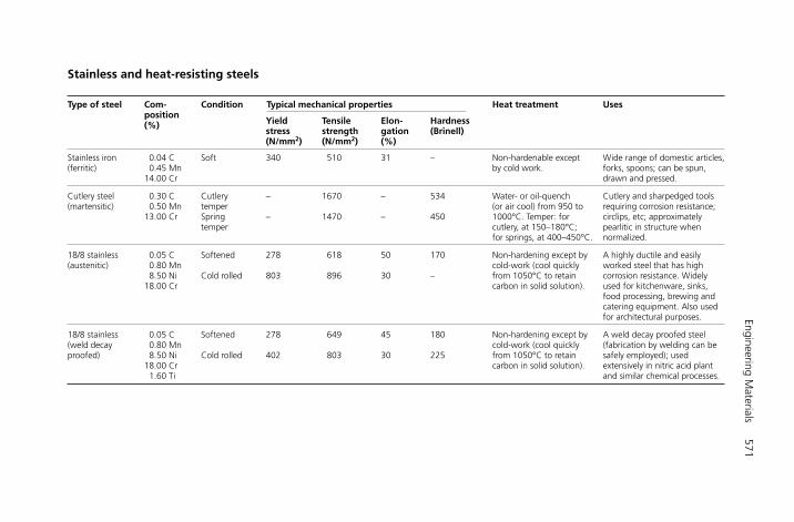
Engineering Materials
571
Stainless and heat-resisting steels
Type of steel Com- Condition Typical mechanical properties Heat treatment Usesposition
Yield Tensile Elon- Hardness (%)stress strength gation (Brinell)(N/mm2) (N/mm2) (%)
Stainless iron 0.04 C Soft 340 510 31 – Non-hardenable except Wide range of domestic articles, (ferritic) 0.45 Mn by cold work. forks, spoons; can be spun,
14.00 Cr drawn and pressed.
Cutlery steel 0.30 C Cutlery – 1670 – 534 Water- or oil-quench Cutlery and sharpedged tools (martensitic) 0.50 Mn temper (or air cool) from 950 to requiring corrosion resistance;
13.00 Cr Spring – 1470 – 450 1000°C. Temper: for circlips, etc; approximately temper cutlery, at 150–180°C; pearlitic in structure when
for springs, at 400–450°C. normalized.
18/8 stainless 0.05 C Softened 278 618 50 170 Non-hardening except by A highly ductile and easily (austenitic) 0.80 Mn cold-work (cool quickly worked steel that has high
8.50 Ni Cold rolled 803 896 30 – from 1050°C to retain corrosion resistance. Widely 18.00 Cr carbon in solid solution). used for kitchenware, sinks,
food processing, brewing and catering equipment. Also used for architectural purposes.
18/8 stainless 0.05 C Softened 278 649 45 180 Non-hardening except by A weld decay proofed steel (weld decay 0.80 Mn cold-work (cool quickly (fabrication by welding can be proofed) 8.50 Ni Cold rolled 402 803 30 225 from 1050°C to retain safely employed); used
18.00 Cr carbon in solid solution). extensively in nitric acid plant 1.60 Ti and similar chemical processes.
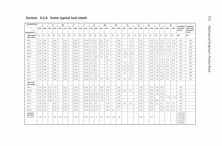
572M
echanical Engineer’s Pocket Book
Composition
Designation
C Si Mn P S Cr Mo
min. max. min. max. min. max. min. max. min. max. min. max. min. max.
High-speed % % % % % % % % % % % % % %tool steels
BM1 0.75 0.85 0.40 0.40 0.035 0.035 3.75 4.5 8.0 9.0
BM2 0.82 0.92 0.40 0.40 0.035 0.035 3.75 4.5 4.75 5.5
BM4 1.25 1.40 0.40 0.40 0.035 0.035 3.75 4.5 4.25 5.0
BM15 1.45 1.60 0.40 0.40 0.035 0.035 4.5 5.0 2.75 3.25
BM35 0.85 0.95 0.40 0.40 0.035 0.035 3.75 4.5 4.75 5.25
BM42 1.0 1.10 0.40 0.40 0.035 0.035 3.5 4.25 9.0 10.0
BT1 0.70 0.80 0.40 0.40 0.035 0.035 3.75 4.5 – 0.70
BT4 0.70 0.80 0.40 0.40 0.035 0.035 3.75 4.5 – 1.0
BT5 0.75 0.85 0.40 0.40 0.035 0.035 3.75 4.5 – 1.0
BT6 0.75 0.85 0.40 0.40 0.035 0.035 3.75 4.5 – 1.0
BT15 1.40 1.60 0.40 0.40 0.035 0.035 4.25 5.0 – 1.0
BT21 0.60 0.70 0.40 0.40 0.035 0.035 3.5 4.25 – 0.7
BT42 1.25 1.40 0.40 0.40 0.035 0.035 3.75 4.5 2.75 3.50
Hot work tool steels
BH10 0.30 0.40 0.75 1.10 0.40 0.035 0.035 2.8 3.2 2.65 2.95
BH10A 0.30 0.40 0.75 1.10 0.40 0.035 0.035 2.8 3.2 2.65 2.95
BH11 0.32 0.42 0.85 1.15 0.40 0.035 0.035 4.75 5.25 1.25 1.75
BH12 0.30 0.40 0.85 1.15 0.40 0.035 0.035 4.75 5.25 1.25 1.75
BH13 0.32 0.42 0.85 1.15 0.40 0.035 0.035 4.75 5.25 1.25 1.75
BH19 0.35 0.45 0.40 0.40 0.035 0.035 4.0 4.5 – 0.45
BH21 0.25 0.35 0.40 0.40 0.035 0.035 2.25 3.25 – 0.60
BH21A 0.20 0.30 0.40 0.40 0.035 0.035 2.25 3.25 – 0.60
Hammer die steelBH 224/5 0.49 0.57 0.35 1.00 0.030 0.025 0.70 1.10 0.25 0.40
–
–
–
–
–
–
–
–
–
–
–
–
–
–
–
–
–
–
–
–
–
–
–
–
–
–
–
–
–
–
–
–
–
–
–
–
–
–
–
–
–
–
–
–
–
–
–
–
–
–
–
–
–
–
–
–
–
–
–
–
–
Section 6.2.6 Some typical tool steels
Ni Co Cu Sn V WAnnealed Hardness
min. max. min. max. min. max. min. max. min. max. min. max. hardness after heat(max.)* treatment
(min.)
% % % % % % % % % % % % HB HV
0.40 1.0† 0.20 0.05 1.0 1.25 1.0 2.0
0.40 1.0† 0.20 0.05 1.75 2.05 6.0 6.75
0.40 1.0† 0.20 0.05 3.75 4.25 5.75 6.5
0.40 4.5 5.5 0.20 0.05 4.75 5.25 6.25 7.0
0.40 4.60 5.20 0.20 0.05 1.75 2.15 6.0 6.75
0.40 7.5 8.5 0.20 0.05 1.0 1.3 1.0 2.0
0.40 1.0† 0.20 0.05 1.0 1.25 17.5 18.5
0.40 4.5 5.5 0.20 0.05 1.0 1.25 17.5 18.5
0.40 9.0 10.0† 0.20 0.05 1.75 2.05 18.5 19.5
0.40 11.25 12.25 0.20 0.05 1.25 1.75 20.0 21.0
0.40 4.5 5.5 0.20 0.05 4.75 5.25 12.0 13.0
0.40 1.0† 0.20 0.05 0.40 0.60 13.5 14.5
0.40 9.0 10.0 0.20 0.05 2.75 3.25 8.5 9.5
0.40 0.20 0.05 0.30 0.50
0.40 2.8 3.2 0.20 0.05 0.30 1.10
0.40 0.20 0.05 0.30 0.50
0.40 0.20 0.05 – 0.50 1.25 1.75
0.40 0.20 0.05 0.90 1.10
0.40 4.0 4.5 0.20 0.05 2.0 2.4 4.0 4.5
0.40 0.20 0.05 – 0.40 8.5 10.0
2.0 2.5 0.20 0.05 – 0.50 8.5 10.0
241
248
255
277
269
269
255
277
290
302
290
255
277
229
241
229
229
229
248
235
255
823
836
849
869
869
897
823
849
869
869
890
798
912
–
–
–
–
–
–
–
–
–
A*444/447A 401/429
1.25 1.80 0.20 0.05 – – B 363/388C 331/352 D 302/321 E 269/293
–
–
–
–
–
–
–
–
–
–
–
–
–
–
–
–
–
–
–
–
–
–
–
–
–
–
–
–
–
–
–
–
–
–
–
–
–
–
–
–
–
–
–
–
–
–
–
–
–
–
–
–
–
–
–
–
–
–
–
–
–
–
–
–
–
–
–
–
–
–
–
–
–
–
–
–
–
–
–
–
–
–
–
–
–
–
–
–
–
–
–
–
–0.70
–
–
–
–
–
–
–
–
–
–
–
–
–
–
–
–
–
–
–
–
–
H6508-Ch06.2.qxd 9/21/05 10:04 AM Page 572
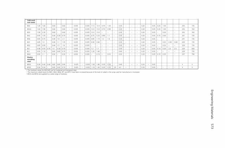
Engineering Materials
573
BD2
BD2A
BD3
BA2
BA6
BO1
BO2
BS1
Cold-worktool steels
* The hardness values for BH224/5 are for hardened and tempered steel.† The maximum cobalt levels for BM1, BM2, BM4, BT1 and BT21 have been increased because of the level of cobalt in the scrap used for manufacture is increased.‡ BP20 and BP30 are supplied to a wide range of hardness.
Plasticsmouldingsteel
BP20
BP30
BL1
BW2
1.40
1.60
1.90
0.95
0.65
0.85
0.85
0.48
0.28
0.26
0.95
0.95
1.60
1.90
2.30
1.05
0.75
1.0
0.95
0.55
0.40
0.34
1.10
1.1
–
–
–
–
–
–
–
0.70
0.40
–
–
–
0.60
0.60
0.60
0.40
0.40
0.40
0.40
1.0
0.60
0.40
0.40
0.30
–
–
–
0.30
1.8
1.1
1.5
0.30
0.65
0.45
0.40
–
0.60
0.60
0.60
0.70
2.1
1.35
1.8
0.70
0.95
0.70
0.70
0.35
–
–
–
–
–
–
–
–
–
–
–
–
0.035
0.035
0.035
0.035
0.035
0.035
0.035
0.035
0.025
0.025
0.035
0.035
–
–
–
–
–
–
–
–
–
–
–
–
0.035
0.035
0.035
0.035
0.035
0.035
0.035
0.035
0.025
0.025
0.035
0.035
11.5
12.0
12.0
4.75
0.85
0.40
–
1.2
1.50
1.10
1.20
–
12.5
13.0
13.0
5.25
1.15
0.60
–
1.7
1.80
1.40
1.60
0.15
1.20
0.90
–
1.1
1.6
–
–
–
0.55
0.35
–
0.10
–
–
–
–
–
–
–
–
–
–
–
–
–
–
–
–
–
–
–
–
–
–
–
–
0.20
0.20
0.20
0.20
0.20
0.20
0.20
0.20
0.25
0.20
0.20
0.20
–
–
–
–
–
–
–
–
–
–
–
–
1.00
1.00
0.50
0.40
–
0.25
0.25
0.30
–
–
0.35
0.40
–
–
–
–
–
–
2.0
–
–
–
0.60
–
–
–
–
–
–
2.5
–
–
–
255
255
255
241
241
229
229
229
‡
‡
229
207
735
763
763
735
735
735
735
600
‡
‡
735
790
–
–
–
–
–
–
–
–
–
3.9
–
–
0.40
0.40
0.40
0.40
0.40
0.40
0.40
0.40
0.40
4.3
0.40
0.20
–
–
–
–
–
–
–
–
–
–
–
–
0.05
0.05
0.05
0.05
0.05
0.05
0.05
0.05
0.05
0.05
0.05
0.05
–
0.25
0.25
–
0.15
–
–
–
0.10
–
0.15
0.70
0.70
–
0.90
1.2
–
–
–
0.35
0.20
–
–

574 Mechanical Engineer’s Pocket Book
6.2.7 Flake (grey), cast irons
Cast iron is the name given to those ferrous metals containing more than 1.7% carbon.Since the maximum amount of carbon which can be held in solid solution as austenite (�-phase) is 1.7%, there will be excess carbon in all cast irons. This can be either taken upby the iron as cementite (combined carbon) or precipitated out as free carbon in the formof graphite flakes (uncombined carbon).
Slow cooling results in coarse gains of ferrite and large flakes of graphite.
More rapid cooling results in both ferrite and pearlite being present together with finerand more uniformly dispersed flakes of graphite. This results in a stronger, tougher andharder cast iron.
Rapid cooling results in very fine flake graphite dispersed throughout a matrix of pearlite.This results in a further increase in strength and hardness.
It is the grey appearance of the freshly fractured surface of cast iron, resulting from theflake graphite, that gives ferritic and pearlitic cast irons the name grey cast irons.
Very rapid cooling and a reduction in silicon content results in all the carbon remainingcombined as pearlite and cementite. Since no grey carbon is visible in the fractured surface,such cast iron is referred to as white cast iron. It is too hard and brittle to be of immediateuse, but white iron castings are used as a basis for the malleable cast irons (see 6.2.11).
As well as iron and carbon the following elements are also present in cast irons:
Silicon This softens the cast iron by promoting the formation of uncombined carbon(graphite) at the expense of combined carbon (cementite). The silicon content is increasedin small castings, which tend to cool rapidly, to promote the formation of ferrite andpearlite, and prevent the formation of excess cementite.
Phosphorus This is a residual impurity from the extraction process. Its presence causesembrittlement and hardness. However, its presence is desirable in complex, decorativecastings, where strength and shock resistance is relatively unimportant, as it increases thefluidity of molten iron.
Sulphur This is also a residual impurity. It stabilizes the cementite and prevents the for-mation of flake graphite, thus hardening the iron. The presence of iron sulphide (FeS)causes embrittlement.
Manganese This is added in small quantities to neutralize the effects of the sulphur. It also refines the grain of the cast iron and so increases its strength. Since excess man-ganese stabilizes the cementite and promotes hardness, the manganese content must bebalanced with the silicon content.
A typical composition for a grey cast iron could be as follows (see also Section 6.2.8):
Carbon 3.3%Silicon 1.5%Manganese 0.75%Sulphur 0.05%Phosphorus 0.5%Iron remainder
H6508-Ch06.2.qxd 9/21/05 10:04 AM Page 574

Engineering Materials 575
6.2.8 BS EN 1561: 1997 Grey cast irons
BS EN 1561 specifies the requirements of seven grades of grey cast iron. Unlike earlierstandards it does not specify the composition or its processing in the foundry. BS EN 1561specifies the properties, test conditions and quality control of the castings. How these areattained are left to the foundry in consultation with the customer. In addition the cus-tomer may specify or require:
(a) a mutually agreed chemical composition;(b) casting tolerances, machining locations;(c) test bars and/or test certificates;(d) whether testing and inspection is to be carried out in the presence of the customer’s
representative;(e) any other requirement such as hardness tests and their locations, non-destructive
tests, and quality assurance.
The main properties of grey cast irons as specified in BS EN 1561 are given in the table onpage 576. Note that for grey cast iron, hardness is not related to tensile strength butvaries with casting section thickness and materials composition.
H6508-Ch06.2.qxd 9/21/05 10:04 AM Page 575
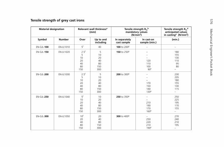
576M
echanical Engineer’s Pocket Book
Material designation Relevant wall thicknessa Tensile strength Rmb Tensile strength Rm
d
(mm) mandatory values anticipated values (N/mm2) in castinge (N/mm2)
Symbol Number Over Up to and In separately In cast-on (min.)including cast sample sample (min.)
EN-GJL-100 EN-JL1010 5f 40 100 to 200g – –
EN-GJL-150 EN-JL1020 2.5f 5 150 to 250g – 1805 10 – 155
10 20 – 13020 40 120 11040 80 110 9580 150 100 80
150 300 90e –
EN-GJL-200 EN-JL1030 2.5f 5 200 to 300g – 2305 10 – 205
10 20 – 18020 40 170 15540 80 150 13080 150 140 115
150 300 130e –
EN-GJL-250 EN-JL1040 5f 10 250 to 350g – 25010 20 – 22520 40 210 19540 80 190 17080 150 170 155
150 300 160e –
EN-GJL-300 EN-JL1050 10f 20 300 to 400g – 27020 40 250 24040 80 220 21080 150 210 195
150 300 190e –
Tensile strength of grey cast irons
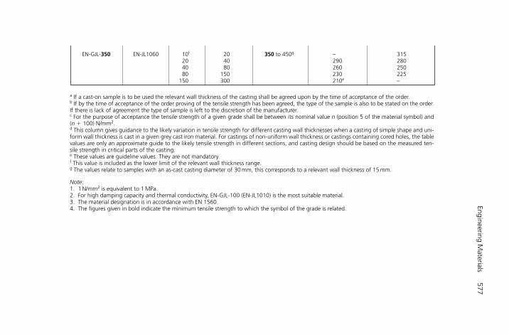
Engineering Materials
577
EN-GJL-350 EN-JL1060 10f 20 350 to 450g – 31520 40 290 28040 80 260 25080 150 230 225
150 300 210e –
a If a cast-on sample is to be used the relevant wall thickness of the casting shall be agreed upon by the time of acceptance of the order.b If by the time of acceptance of the order proving of the tensile strength has been agreed, the type of the sample is also to be stated on the order.If there is lack of agreement the type of sample is left to the discretion of the manufacturer.c For the purpose of acceptance the tensile strength of a given grade shall be between its nominal value n (position 5 of the material symbol) and(n � 100) N/mm2.d This column gives guidance to the likely variation in tensile strength for different casting wall thicknesses when a casting of simple shape and uni-form wall thickness is cast in a given grey cast iron material. For castings of non-uniform wall thickness or castings containing cored holes, the tablevalues are only an approximate guide to the likely tensile strength in different sections, and casting design should be based on the measured ten-sile strength in critical parts of the casting.e These values are guideline values. They are not mandatory.f This value is included as the lower limit of the relevant wall thickness range.g The values relate to samples with an as-cast casting diameter of 30 mm, this corresponds to a relevant wall thickness of 15 mm.
Note: 1. 1 N/mm2 is equivalent to 1 MPa.2. For high damping capacity and thermal conductivity, EN-GJL-100 (EN-JL1010) is the most suitable material.3. The material designation is in accordance with EN 1560.4. The figures given in bold indicate the minimum tensile strength to which the symbol of the grade is related.

578 Mechanical Engineer’s Pocket Book
Material designation Relevant wall thickness (mm) Brinell hardnessa,b
(HB 30)
Symbol Number Over Up to and min. max.including
EN-GJL-HB155 EN-JL2010 40c 80 – 15520 40 – 16010 20 – 1705 10 – 1852.5 5 – 210
EN-GJL-HB175 EN-JL2020 40c 80 100 17520 40 110 18510 20 125 2055 10 140 2252.5 5 170 260
EN-GJL-HB195 EN-JL2030 40c 80 120 19520 40 135 21010 20 150 2305 10 170 2604 5 190 275
EN-GJL-HB215 EN-JL2040 40c 80 145 21520 40 160 23510 20 180 2555 10 200 275
EN-GJL-HB235 EN-JL2050 40c 80 165 23520 40 180 25510 20 200 275
EN-GJL-HB255 EN-JL2060 40c 80 185 25520 40 200 275
Brinell hardness of castings of grey cast iron, mandatory and anticipated values at the agreed test position
a For each grade, Brinell hardness decreases with increasing wall thickness.b By agreement between the manufacturer and the purchaser a narrower hardness range may beadopted at the agreed position on the casting, provided that this is not less than 40 Brinell hardnessunits. An example of such a circumstance could be castings for long series production.c Reference relevant wall thickness for the grade.
Note:1. Information on the relationship between Brinell hardness and tensile strength is indicated in Figure
B.1 and the relationship between Brinell hardness and relevant wall thickness in Figure C.2 ofAnnexes B and C, respectively (see: BS EN 1561).
2. The material designation is in accordance with EN 1560.3. The figures given in bold indicate the minimum and maximum Brinell hardness, to which the sym-
bol of the grade is related and the corresponding reference relevant wall thickness range limits.
H6508-Ch06.2.qxd 9/21/05 10:04 AM Page 578
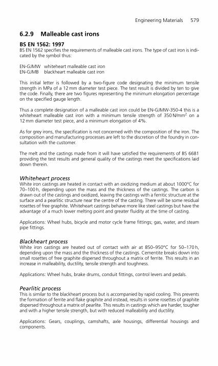
Engineering Materials 579
6.2.9 Malleable cast irons
BS EN 1562: 1997BS EN 1562 specifies the requirements of malleable cast irons. The type of cast iron is indi-cated by the symbol thus:
EN-GJMW whiteheart malleable cast ironEN-GJMB blackheart malleable cast iron
This initial letter is followed by a two-figure code designating the minimum tensilestrength in MPa of a 12 mm diameter test piece. The test result is divided by ten to givethe code. Finally, there are two figures representing the minimum elongation percentageon the specified gauge length.
Thus a complete designation of a malleable cast iron could be EN-GJMW-350-4 this is awhiteheart malleable cast iron with a minimum tensile strength of 350 N/mm2 on a12 mm diameter test piece, and a minimum elongation of 4%.
As for grey irons, the specification is not concerned with the composition of the iron. Thecomposition and manufacturing processes are left to the discretion of the foundry in con-sultation with the customer.
The melt and the castings made from it will have satisfied the requirements of BS 6681providing the test results and general quality of the castings meet the specifications laiddown therein.
Whiteheart processWhite iron castings are heated in contact with an oxidizing medium at about 1000°C for70–100 h, depending upon the mass and the thickness of the castings. The carbon isdrawn out of the castings and oxidized, leaving the castings with a ferritic structure at thesurface and a pearlitic structure near the centre of the casting. There will be some residualrosettes of free graphite. Whiteheart castings behave more like steel castings but have theadvantage of a much lower melting point and greater fluidity at the time of casting.
Applications: Wheel hubs, bicycle and motor cycle frame fittings; gas, water, and steampipe fittings.
Blackheart processWhite iron castings are heated out of contact with air at 850–950°C for 50–170 h,depending upon the mass and the thickness of the castings. Cementite breaks down intosmall rosettes of free graphite dispersed throughout a matrix of ferrite. This results in anincrease in malleability, ductility, tensile strength and toughness.
Applications: Wheel hubs, brake drums, conduit fittings, control levers and pedals.
Pearlitic processThis is similar to the blackheart process but is accompanied by rapid cooling. This preventsthe formation of ferrite and flake graphite and instead, results in some rosettes of graphitedispersed throughout a matrix of pearlite. This results in castings which are harder, tougherand with a higher tensile strength, but with reduced malleability and ductility.
Applications: Gears, couplings, camshafts, axle housings, differential housings and components.
H6508-Ch06.2.qxd 9/21/05 10:04 AM Page 579

580 Mechanical Engineer’s Pocket Book
Mechanical properties of whiteheart malleable cast irons
Material designation Nominal Tensile Elongation 0.2% Brinell diameter strength A3.4 (%) proof hardness
of Rm min. stress (for test (N/mm2) Rp0.2 information
piece min. (N/mm2) only)Symbol Number d (mm) min. HB max.
6 270 10 –9 310 5 –
EN-GJMW-350-4 EN-JM1010 12 350 4 – 23015 360 3 –
6 280 16 –a
9 320 15 170EN-GJMW-360-12b EN-JM1020b 12 360 12 190 200
15 370 7 200
6 300 12 –a
9 360 8 200EN-GJMW-400-5 EN-JM1030 12 400 5 220 220
15 420 4 230
6 330 12 –a
9 400 10 230EN-GJMW-450-7 EN-JM1040 12 450 7 260 220
15 480 4 280
6 – – –a
9 490 5 310EN-GJMW-550-4 EN-JM1050 12 550 4 340 250
15 570 3 350
a Due to the difficulty in determining the proof stress of small test pieces, the values and the methodof measurement shall be agreed between the manufacturer and the purchaser at the time of accept-ance of the order.b Material most suitable for welding.
Note:1. 1 N/mm2 is equivalent to 1 MPa.2. The material designation is in accordance with EN 1560.3. The figures given in bold indicate the minimum tensile strength and minimum elongation A3.4
to which the symbol of the grade is related, and the preferred nominal diameter of the test pieceand the corresponding minimum 0.2% proof stress.
H6508-Ch06.2.qxd 9/21/05 10:04 AM Page 580

Engineering Materials
581
Material designation Nominal Tensile Elongation 0.2% proof Brinell hardness diameter of strength A3.4 (%) min. stress Rp0.2 (for informationtest piecea Rm (N/mm2) (N/mm2) min. only) HB
Symbol Number d (mm) min.
EN-GJMB-300-6b EN-JM1110b 12 or 15 300 6 – 150 maximum
EN-GJMB-350-10 EN-JM1130 12 or 15 350 10 200 150 maximum
EN-GJMB-450-6 EN-JM1140 12 or 15 450 6 270 150 to 200
EN-GJMB-500-5 EN-JM1150 12 or 15 500 5 300 165 to 215
EN-GJMB-550-4 EN-JM1160 12 or 15 550 4 340 180 to 230
EN-GJMB-600-3 EN-JM1170 12 or 15 600 3 390 195 to 245
EN-GJMB-650-2 EN-JM1180 12 or 15 650 2 430 210 to 260
EN-GJMB-700-2 EN-JM1190 12 or 15 700 2 530 240 to 290
EN-GJMB-800-1 EN-JM1200 12 or 15 800 1 600 270 to 320
a Where a 6 mm diameter test piece is representative of the relevant wall thickness of a casting, this size of the test piece may be used byagreement between the manufacturer and the purchaser at the time of acceptance of the order. The minimum properties given in this tableshall apply.b Material intended particularly for applications in which pressure tightness is more important than a high degree of strength and ductility.
Note: 1. 1 N/mm2 is equivalent to 1 MPa.2. The material designation is in accordance with EN 1560.3. The figures given in bold are related to the minimum tensile strength and minimum elongation A3.4 of the grade.
Mechanical properties of blackheart malleable cast irons

582 Mechanical Engineer’s Pocket Book
6.2.10 Spheroidal graphite cast irons
Spheroidal graphite cast iron is also known as nodular cast iron, ductile cast iron, high-duty cast iron, etc.
The addition of magnesium or cerium to molten grey cast iron prevents the formation offlake graphite upon cooling and solidification. Instead, the uncombined carbon is distrib-uted as fine spheroids throughout the mass of the casting. This results in a more homoge-neous structure having greater strength and ductility and less susceptibility to fatigue failure.
BS EN 1563: 1997: Spheroidal graphite cast ironsBS EN 1563 specifies the requirements for spheroidal or nodular graphite cast irons. Again,the standard does not specify the chemical composition of the iron, its method of manu-facture or any subsequent heat treatment. The standard is solely concerned with the prop-erties, testing and quality control of the finished castings. How this is attained is left to thediscretion of the foundry in consultation with the customer. It is a very comprehensive stan-dard and it is only possible to review briefly some of its more important points within thescope of this chapter. The standard itself should be consulted for more detailed study.
Mechanical properties measured on test pieces machined from separately cast samples
Material designation Tensile 0.2% s Elongationstrength proof stress A
Rm Rp0.2 (%)Symbol Number (N/mm2) (N/mm2) min.
min. min.
EN-GJS-350-22-LTa EN-JS1015 350 220 22
EN-GJS-350-22-RTb EN-JS1014 350 220 22
EN-GJS-350-22 EN-JS1010 350 220 22
EN-GJS-400-18-LTa EN-JS1025 400 240 18
EN-GJS-400-18-RTb EN-JS1024 400 250 18
EN-GJS-400-18 EN-JS1020 400 250 18
EN-GJS-400-15 EN-JS1030 400 250 15
EN-GJS-450-10 EN-JS1040 450 310 10
EN-GJS-500-7 EN-JS1050 500 320 7
EN-GJS-600-3 EN-JS1060 600 370 3
EN-GJS-700-2 EN-JS1070 700 420 2
EN-GJS-800-2 EN-JS1080 800 480 2
EN-GJS-900-2 EN-JS1090 900 600 2
a LT for low temperature.b RT for room temperature.
Note:1. The values for these materials apply to castings cast in sand moulds of comparable thermal dif-
fusivity. Subject to amendments to be agreed upon in the order, they can apply to castingsobtained by alternative methods.
2. Whatever the method used for obtaining the castings, the grades are based on the mechanicalproperties measured on test pieces taken from samples separately cast in a sand mould or amould of comparable thermal diffusivity.
3. 1 N/mm2 is equivalent to 1 MPa.4. The material designation is in accordance with EN 1560.
H6508-Ch06.2.qxd 9/21/05 10:04 AM Page 582
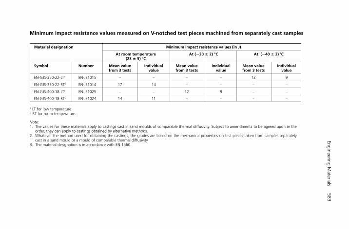
Engineering Materials
583
Minimum impact resistance values measured on V-notched test pieces machined from separately cast samples
Material designation Minimum impact resistance values (in J)
At room temperature At (�20 � 2) °C At (�40 � 2) °C(23 � 5) °C
Symbol Number Mean value Individual Mean value Individual Mean value Individual from 3 tests value from 3 tests value from 3 tests value
EN-GJS-350-22-LTa EN-JS1015 – – – – 12 9
EN-GJS-350-22-RTb EN-JS1014 17 14 – – – –
EN-GJS-400-18-LTa EN-JS1025 – – 12 9 – –
EN-GJS-400-18-RTb EN-JS1024 14 11 – – – –
a LT for low temperature.b RT for room temperature.
Note:1. The values for these materials apply to castings cast in sand moulds of comparable thermal diffusivity. Subject to amendments to be agreed upon in the
order, they can apply to castings obtained by alternative methods.2. Whatever the method used for obtaining the castings, the grades are based on the mechanical properties on test pieces taken from samples separately
cast in a sand mould or a mould of comparable thermal diffusivity.3. The material designation is in accordance with EN 1560.

584 Mechanical Engineer’s Pocket Book
6.2.11 Alloy cast ironsThe alloying elements in cast irons are similar to those in alloy steels:
Nickel is used for grain refinement, to add strength and to promote the formation of freegraphite. Thus it toughens the casting.
Chromium stabilizes the combined carbon (cementite) present and thus increases thehardness and wear resistance of the casting. It also improves the corrosion resistance ofthe casting, particularly at elevated temperatures. As in alloy steels, nickel and chromiumtend to be used together. This is because they have certain disadvantages when used sep-arately which tend to offset their advantages. However, when used together the disad-vantages are overcome whilst the advantages are retained.
Copper is used very sparingly as it is only slightly soluble in iron. However, it is useful inreducing the effects of atmospheric corrosion.
Vanadium is used in heat-resisting castings as it stabilizes the carbides and reduces theirtendency to decompose at high temperatures.
Molybdenum dissolves in the ferrite and, when used in small amounts (0.5%), itimproves the impact strength of the casting. It also prevents ‘decay’ at high temperaturesin castings containing nickel and chromium. When molybdenum is added in largeramounts it forms double carbides, increases the hardness of castings with thick sections,and also promotes uniformity of the microstructure.
Martensitic cast irons contain between 4% and 6% nickel and approximately 1%chromium (e.g. Ni-hard cast iron). This is naturally martensitic in the cast state but, unlikealloys with rather less nickel and chromium, it does not need to be quench hardened, thusreducing the possibility of cracking and distortion. It is used for components which needto resist abrasion. It can only be machined by grinding.
Austenitic cast irons contain between 11% and 20% nickel and up to 5% chromium.These alloys are corrosion resistant, heat resistant, tough, and non-magnetic.
Since the melting temperatures of alloy cast irons can be substantially higher than those forcommon grey cast irons, care must be taken in the selection of moulding sands and thepreparation of the surfaces of the moulds. Increased venting of the moulds is also required asthe higher temperatures cause more rapid generation of steam and gases. The furnace andcrucible linings must also be suitable for the higher temperatures and the inevitable increasein maintenance costs is also a significant factor when working with high alloy cast irons.
The growth of cast irons is caused by the breakdown of pearlitic cementite into ferrite andgraphite at approximately 700°C. This causes an increase in volume. This increase in vol-ume is further aggravated by hot gases penetrating the graphite cavities and oxidizing theferrite grains. This volumetric growth causes warping and the setting up of internalstresses leading to cracking, particularly at the surface. Therefore, where castings arecalled upon to operate at elevated temperatures, alloy cast irons should be used. A lowcost alloy is Silal which contains 5% silicon and a relatively low carbon content. The lowcarbon content results in a structure which is composed entirely of ferrite and graphitewith no cementite present. Unfortunately Silal is rather brittle because of the high siliconcontent. A more expensive alloy is Nicrosilal. This is an austenitic nickel-chromium alloywhich is much superior in all respects for use at elevated temperatures.
Three typical alloy cast irons are listed in Section 6.2.12 together with their properties,composition and some uses.
H6508-Ch06.2.qxd 9/21/05 10:04 AM Page 584

Engineering Materials 585
6.2.12 Composition, properties and uses of some typical cast irons
Type of iron Composition Representative mechanical properties(%)
Tensile strength Hardness Uses(N/mm2) (Brinell)
Grey iron 3.30 C Strengths vary Motor vehicle 1.90 Si with sectional brake drums.0.65 Mn thickness but are 0.10 S generally in the range 0.15 P 150–350 N/mm2.
Grey iron 3.25 C – Motor vehicle 2.25 Si cylinders and 0.65 Mn pistons.0.10 S0.15 P
Grey iron 3.25 C Strengths vary with – Heavy machine 1.25 Si sectional thickness castings.0.50 Mn but are generally 0.10 S in the range 10.35 P 50–350 N/mm2.
Phosphoric 3.60 C – Light and medium grey iron 1.75 Si water pipes.
0.50 Mn0.10 S0.80 P
Chromidium 3.20 C 275 230 Cylinder blocks, 2.10 Si brake drums, 0.80 Mn clutch casings, etc.0.05 S0.17 P0.32 Cr
Wear and 2.90 C 450 300 Crankshafts for shock 2.10 Si diesel and petrol resistant 0.70 Mn engines (good
0.05 S strength, shock 0.10 P resistance and 1.75 Ni vibration damping 0.10 Cr capacity).0.80 Mo0.15 Cu
Ni-resist 2.90 C 215 130 Pump castings 2.10 Si handling 1.00 Mn concentrated 0.05 S chloride solutions: 0.10 P an austenitic
15.00 Ni corrosion resistant 2.00 Cr alloy.6.00 Cu
�
H6508-Ch06.2.qxd 9/21/05 10:04 AM Page 585

586 Mechanical Engineer’s Pocket Book
6.3 Non-ferrous metals and alloys
6.3.1 Non-ferrous metals and alloys – introduction
Non-ferrous metals are all the known metals other than iron. Few of these metals areused in the pure state by engineers because of their relatively low strengths; two notableexceptions are copper and aluminium. Mostly they are used as the bases and alloying elem-ents in both ferrous and non-ferrous alloys. Some non-ferrous metals are used for corro-sion resistant coatings: for example, galvanized iron (zinc coated, low-carbon steel) andtinplate (tin coated, low-carbon steel).
It is not possible within the scope of this book to consider the composition and propertiesof the very large range of non-ferrous materials available. The following sections are,therefore, only an introduction to the composition and properties of some of the morewidely used non-ferrous metals and alloys. For further information the wide range ofBritish Standards relating to non-ferrous metals and alloys should be consulted, as shouldbe the comprehensive manuals published by the metal manufacturers and their tradeassociations (e.g. Copper Development Association).
Only a limited number of non-ferrous alloys can be hardened by heat treatment. Themajority can only be work-hardened by processing (e.g. cold rolling). Thus the conditionof the metal, as the result of processing, has an important effect upon its properties, aswill be shown in the following sections.
Other notable non-ferrous alloys, which are not included in this section, but which shouldbe considered are:
Magnesium alloys (Elektron): used for ultra-lightweight castings.Nickel alloys (Nimonic): high-temperature-resistant alloys, used in jet engines and gas turbines.Zinc-based alloys (Mazak): used for pressure die-casting alloys.
6.3.2 High copper content alloys
Silver copperThe addition of 0.1% silver to high-conductivity copper raises the annealing temperatureby 150°C with minimal loss of conductivity. This avoids hard drawn copper componentssoftening when conductors are being soldered to them.
Cadmium copperLike silver, cadmium has little effect upon the conductivity of the copper. Cadmiumstrengthens, toughens, and raises the tempering temperature of copper. Cadmium cop-per is widely used for medium- and low-voltage overhead conductors, overhead tele-phone and telegraph wires, and the overhead conductors for electrified railways. In theannealed condition it has high flexibility and is used for aircraft wiring where its ability towithstand vibration without failing in fatigue is an important safety factor.
Chromium copperA typical alloy contains 0.5% chromium. It is one of the few non-ferrous alloys which canbe heat treated. Thus it can be manipulated and machined in the ductile condition andsubsequently hardened and strengthened by heating to 500°C for approximately 2 h. Ithas a relatively low conductivity compared with silver copper and cadmium copper.
Tellurium copperThe addition of 0.5% tellurium makes the copper as machineable as free-cutting brasswhilst retaining its high conductivity. It also improves the very high corrosion resistance ofcopper. Tellurium copper is widely used in electrical machines and switchgear in hostileenvironments such as mines, quarries and chemical plants. The addition of traces nickeland silicon makes tellurium copper heat treatable, but with some loss of conductivity.
H6508-Ch06.3a.qxd 9/12/05 4:54 PM Page 586

Beryllium copperThis is used where mechanical rather than electrical properties are required. Beryllium copperis softened by heating it to 800°C and quenching it in water. In this condition it is soft andductile and capable of being extensively cold worked. It can be hardened by reheating to300–320°C for upwards of 2 h. The resulting mechanical properties will depend on the extentof the processing (cold working) received prior to reheating. Beryllium copper is widely usedfor instrument springs, flexible metal bellows and corrugated diaphragms for aneroid barom-eters and altimeters, and for the Bourdon tubes in pressure gauges. Hand tools made fromberyllium copper are almost as strong as those made from steel, but will not strike sparksfrom other metals or from flint stones. Thus tools made from beryllium copper alloy are usedwhere there is a high risk of explosion (e.g. mines, oil refineries, oil rigs and chemical plants).
6.3.3 Wrought copper and copper alloys: condition code
O Material in the annealed condition (soft)M Material in the ‘as-manufactured’ condition1⁄4H Material with quarter-hard temper (due to cold working)1⁄2H Material with half-hard temperH Material with fully hard temperEH Material with extra-hard temperSH Material with spring-hard temperESH Material with extra-spring-hard temper.
The above are listed in order of ascending hardness.
Materials which have acquired a hard temper due to cold working can have their hardnessreduced and their ductility increased by heat treatment (e.g. annealing or solution treatment).
Chemical symbols used in the following tables:Al aluminium Co cobalt Ni nickel Si siliconAr arsenic Cr chromium P phosphorus Sn tinBe beryllium Cu copper Pb lead Te telleriumBi bismuth Fe iron S sulphur Ti titaniumC calcium Mg magnesium Sb antimony Zn zincCd cadmium Mn manganese Se selenium Zr zirconium
6.3.4 British Standards relating copper and copper alloys
British Standard BS 2874 Copper and copper alloy rods and sections (chemical compos-ition and mechanical properties) relating to copper and copper alloys is now obsolescentand should not be specified for new designs although the materials listed within thisStandard will continue to be available and be used for some time to come.
The replacement standards are as follows. They are very detailed and comprehensive andit is not physically possible to reproduce them within the confines of this Pocket Book.
● BS EN 12163: 1998 – Copper and copper alloys (rod for general purposes).● BS EN 12167: 1998 – Copper and copper alloys for profiles and rectangular bar for
general purposes.● BS EN 1652: 1997 – Copper and copper alloys for plate, sheet and circles for general
purposes.● BS EN 1653: 1998 – Copper and copper alloys for plate sheet and circles for boilers,
pressure vessels and hot water storage units.● BS EN 1982: 1998 – Copper and copper alloys for ingots and casting.
The following copper and copper alloy materials listed in Sections 6.3.5–6.3.26 inclusiveare for guidance only.
Engineering Materials 587
H6508-Ch06.3a.qxd 9/12/05 4:54 PM Page 587
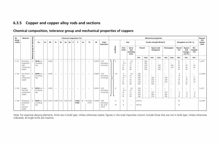
BS Material Chemical composition (%) Mechanical properties Nearest desig- ISO nation Cu Sn Pb Fe Ni As Sb S P Se Te Bi Total Size Tensile strength (N/mm2) Elongation on 5.65 �So design-
impurities ation
Over Up to Round Square and Rectangular Round Square Rec-(mm) and hexagonal (%) and tangular
Including hexago- (%)(mm) nal (%)
min. max. min. max. min. max. min. min. min.
C 101 Electrolytic I 99.90 min. – 0.005 – – – – – – – – 0.0010 0.03 0 4 6.3 – 260 – – – – 32 – – Cu-ETPtough pitch (including (excluding 6.3 10 – 250 – – – – 32 – –high- Ag) 0 and Ag) 10 12 – 240 – 240 – 240 40 40 40conductivity 12 50 – 230 – 230 – 230 45 45 45copper 50 80 – 230 – 230 – – 45 45 –
C 102 Fire refined I 99.90 min. – 0.005 – – – – – – – – 0.0025 0.04 1⁄2H 4 6.3 290 – – – – – 4 – – Cu-FRHChigh- (including (excluding 6.3 10 280 – – – – – 8 – –conductivity Ag) O and Ag) 10 12 260 – 260 – 250 – 12 12 12copper 12 25 250 – 250 – 230 – 18 18 18
25 50 230 – 230 – 230 – 22 22 1850 80 230 – 230 – – – 22 22 –
C 103 Oxygen- I 99.95 min. – 0.005 – – – – – – – – 0.0010 0.03 H 4 6.3 350 – – – – – – – – Cu-OFfree high- (including (excluding 6.3 10 350 – – – – – – – –conductivity Ag) O and Ag) 10 12 320 – 310 – 270 – 6 6 6copper 12 25 290 – 280 – 260 – 8 8 8
25 50 260 – 250 – 250 – 12 12 10
C 106 Phosphorus I 99.85 min. 0.01 0.010 0.030 0.10 0.05 0.01 – 0.013– Se � Te 0.020– 0.0030 0.06 O 6 – 210 min. 33 Cu-DHPdeoxidized (including 0.050 0.010 (excludingnon- Ag) Ag. As Ni M 6 – 230 min. 13arsenical and P)copper
Mat
eria
l gro
up
fo
r to
lera
nce
s
Co
nd
itio
n
6.3.5 Copper and copper alloy rods and sections
Chemical composition, tolerance group and mechanical properties of coppers
� �Note: For essential alloying elements, limits are in bold type. Unless otherwise stated, figures in the total impurities column include those that are not in bold type. Unless otherwiseindicated, all single limits are maxima.

BS Material Material Chemical composition (%) Mechanical properties Nearestdesig- group of ISOnation tolerances Cu Ni P Te Cr Co Be Zr Bi Fe Sb Si S Sn Total Cond- Size Tensile 0.2% Elongation designa-
impurities ition strength proof on 5.65 tion(N/mm2) stress �
___So
(N/mm2)
Over Up to and min. min. min.(mm) including
(mm)
C 109 Copper I Rem. – – 0.30– – – – – – – – – – – 0.2 O 6 – 210 – 28 CuTetellurium 0.70
M 6 50 260 – 850 – 240 – 8
C 111 Copper– I Rem. – – – – – – – – – – – 0.3–0.6 – 0.2 O 6 – 210 – 28 CuSsulphur
M 6 50 260 – 850 – 240 – 8
C 112 Copper– II Rem. Ni � Fe – – – 2.0– 0.4– – – 0.10 – 0.2 – – 0.05 cobalt– 0.5 2.8 0.7 (excluding TH – – 690 – 9 CuCo2Beberyllium Fe, Ni and
Si)
C 113 Copper– II Rem. 0.8– 0.16– – – – – – – – – – 0.2 – 0.03 TH – 25 410 – 18nickel– 1.2 0.25 (excluding 25 – 390 – 20phosphorus S)
CC 101 Copper– II Rem. 0.02 0.01 – 0.3– – – – 0.001 0.08 0.002 0.2 0.08 0.008 0.05 TH – 25 410 – 15 CuCr1chromium 1.4 (excluding 25 – 370 – 15
Fe, Si andS)
CC 102 Copper– II Rem. 0.02 0.01 – 0.5– – – 0.02– 0.001 0.08 0.002 0.2 – 0.008 0.05 TH – 25 410 – 15 CuCr1Zrchromium– 1.4 0.2 (excluding 25 – 370 – 15zirconium Fe and Si)
Chemical composition, tolerance group and mechanical properties of alloyed coppers (continued )
Note: For essential alloying elements, limits are in bold type. Unless otherwise stated, figures in the total impurities column include those that are not in bold type. Unless otherwise indi-cated, all single limits are maxima.
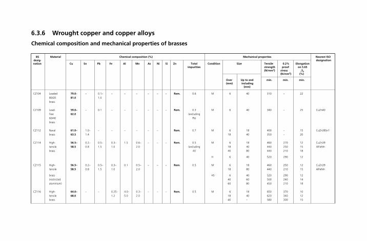
BS Material Chemical composition (%) Mechanical properties Nearest ISO desig- designationnation Cu Sn Pb Fe Al Mn As Ni Si Zn Total Condition Size Tensile 0.2% Elongation
impurities strength proof on 5.65(N/mm2) stress �So
(N/mm2) (%)
Over Up to and min. min. min.(mm) including
(mm)
CZ104 Leaded 79.0– – 0.1– – – – – – – Rem. 0.6 M 6 40 310 – 22
80/20 81.0 1.0
brass
CZ109 Lead- 59.0– – 0.1 – – – – – – Rem. 0.3 M 6 40 340 – 25 CuZn40
free 62.0 (excluding
60/40 Pb)
brass
CZ112 Naval 61.0– 1.0– – – – – – – Rem. 0.7 M 6 18 400 – 15 CuZn38Sn1
brass 63.5 1.4 18 40 350 – 20
CZ114 High- 56.5– 0.2– 0.5– 0.3– 1.5 0.6– – – – Rem. 0.5 M 6 18 460 270 12 CuZn39
tensile 58.5 0.8 1.5 1.0 2.0 (excluding 18 40 440 250 15 AlFeMn
brass Al) 40 80 440 210 18
H 6 40 520 290 12
CZ115 High- 56.5– 0.2– 0.5– 0.3– 0.1 0.5– – – – Rem. 0.5 M 6 18 460 250 12 CuZn39
tensile 58.5 0.8 1.5 1.0 2.0 18 80 440 210 15 AlFeMn
brass HS 6 40 520 290 12
(restricted 40 60 500 240 14
aluminium) 60 80 450 210 18
CZ116 High- 64.0– – – 0.25– 4.0– 0.3– – – – Rem. 0.5 M 6 18 650 370 10
tensile 68.0 1.2 5.0 2.0 18 40 620 340 12
brass 40 – 580 300 15
6.3.6 Wrought copper and copper alloys
Chemical composition and mechanical properties of brasses
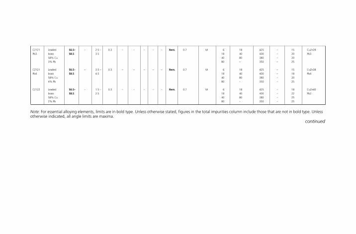
CZ121 Leaded 56.5– – 2.5 – 0.3 – – – – – Rem. 0.7 M 6 18 425 – 15 CuZn39
Pb3 brass 58.5 3.5 18 40 400 – 20 Pb3
58% Cu 40 80 380 – 20
3% Pb 80 – 350 – 25
CZ121 Leaded 56.5– – 3.5 – 0.3 – – – – – Rem. 0.7 M 6 18 425 – 15 CuZn38
Pb4 brass 58.5 4.5 18 40 400 – 18 Pb4
58% Cu 40 80 380 – 20
4% Pb 80 – 350 – 25
CZ122 Leaded 56.5– – 1.5 – 0.3 – – – – – Rem. 0.7 M 6 18 425 – 18 CuZn40
brass 58.5 2.5 18 40 400 – 22 Pb2
58% Cu 40 80 380 – 25
2% Pb 80 – 350 – 25
Note: For essential alloying elements, limits are in bold type. Unless otherwise stated, figures in the total impurities column include those that are not in bold type. Unlessotherwise indicated, all angle limits are maxima.
continued
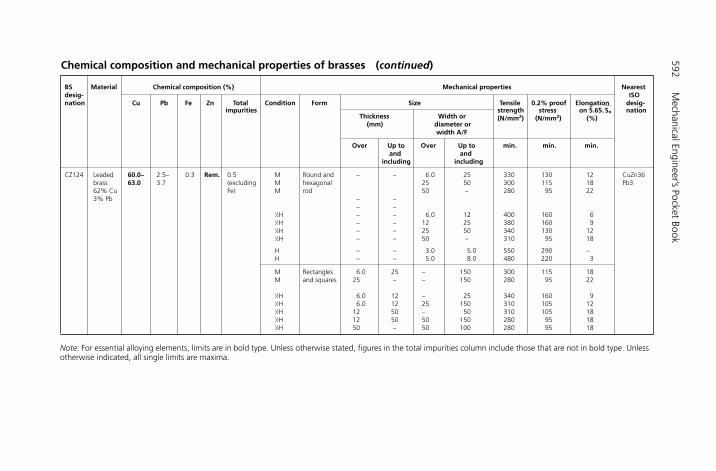
592M
echanical Engineer’s Pocket Book
BS Material Chemical composition (%) Mechanical properties Nearestdesig- ISOnation Cu Pb Fe Zn Total Condition Form Size Tensile 0.2% proof Elongation desig-
impuritiesThickness Width or
strength stress on 5.65�__So nation
(mm) diameter or(N/mm2) (N/mm2) (%)
width A/F
Over Up to Over Up to min. min. min.and and
including including
CZ124 Leaded 60.0– 2.5– 0.3 Rem. 0.5 M Round and – – 6.0 25 330 130 12 CuZn36brass 63.0 3.7 (excluding M hexagonal 25 50 300 115 18 Pb362% Cu Fe) M rod 50 – 280 95 223% Pb – –
– –1⁄2H – – 6.0 12 400 160 61⁄2H – – 12 25 380 160 91⁄4H – – 25 50 340 130 121⁄2H – – 50 – 310 95 18
H – – 3.0 5.0 550 290 –H – – 5.0 8.0 480 220 3
M Rectangles 6.0 25 – 150 300 115 18M and squares 25 – – 150 280 95 22
1⁄2H 6.0 12 – 25 340 160 91⁄2H 6.0 12 25 150 310 105 121⁄2H 12 50 – 50 310 105 181⁄2H 12 50 50 150 280 95 181⁄2H 50 – 50 100 280 95 18
Chemical composition and mechanical properties of brasses (continued)
Note: For essential alloying elements, limits are in bold type. Unless otherwise stated, figures in the total impurities column include those that are not in bold type. Unlessotherwise indicated, all single limits are maxima.
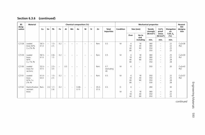
Engineering Materials
593
Section 6.3.6 (continued)
BS Material Chemical composition (%) Mechanical properties Nearestdesig- ISOnation Cu Sn Pb Fe AI Mn As Ni Si Zn Total Condition Size (mm) Tensile 0.2% Elongation designa-
impurities strength proof on tion
Over Up to(N/mm2) stress 5.65�So
and (N/mm2) (%)
including min. min. min.
CZ128 Leaded 58.5– – 1.5– 0.2 – – – – – Rem. 0.5 M 6 18 380 – 22 CuZn38brass 60% 61.0 2.5 18 40 380 – 22 Pb2Cu 2% Pb 40 80 350 – 25
80 – 350 – 25
CZ129 Leaded 58.5– – 0.8– 0.2 – – – – – Rem. 0.5 M 6 18 380 – 25 CuZn39brass 61.0 1.5 18 40 380 – 25 Pb160% 40 80 350 – 28Cu 1% Pb 80 – 350 – 28
CZ130 Leaded 55.5– – 2.5– – 0.5 – – – Rem. 0.7 M 6 – 350 – 20 CuZn43brass for 57.5 3.5 (excluding Pb2sections Al)
CZ131 Leaded 61.0– – 1.5– 0.2 – – – – – Rem. 0.5 M 6 18 350 – 22 CuZn37brass 63.0 2.5 18 40 350 – 25 Pb262% Cu 40 80 350 – 282% Pb 80 – 330 – 28
CZ132 Dezincification Rem. 0.2 1.7– 0.2 – – 0.08– – – 35.0– 0.5 O 6 – 280 – 30resistant 2.8 0.15 37.0brass M 6 18 380 – 20
18 40 350 – 2240 80 350 – 25
continued
594M
echanical Engineer’s Pocket Book
BS Material Chemical composition (%) Mechanical properties Nearestdesig- ISOnation Cu Sn Pb Fe AI Mn As Ni SI Zn Total Condition Size (mm) Tensile 0.2% Elongation designa-
impurities strength proof on tion
Over Up to(N/mm2) stress 5.65�So
and (N/mm2) (%)
including min. min. min.
CZ133 Naval 59.0– 0.50– 0.20 0.10 – – – – – Rem. 0.4 M 6 18 400 170 20brass 62.0 1.0 18 40 350 150 25(uninhibited)
CZ134 Naval 59.0– 0.50– 1.3– 0.10 – – – – – Rem. 0.2 M 6 18 400 170 15brass 62.0 1.0 2.2 18 40 350 150 20(high leaded)
CZ135 High-tensile 57.0– 0.3 0.8 0.5 1.0– 1.5– – 0.2 0.3– Rem. 0.5 M 6 40 550 270 12 CuZn37brass with 60.0 2.0 3.5 1.3 (excluding Mn3 Al2Sisilicon) Sn, Pb,
Fe and Ni)
CZ136 Manganese 56.0– – 3.0 – – 0.5– – – – Rem. 0.7 M 6 18 380 – 20brass 59.0 1.5 (excluding 18 40 350 – 25
Pb)
CZ137 Leaded 58.5– – 0.3– 0.2 – – – – – Rem. 0.5 M 6 40 380 – 25 CuZn40Pbbrass 61.0 0.8 40 – 350 – 2860% Cu0.5% Pb
NS101 Leaded 10% 44.0– – 1.0– 0.4 – 0.2– – 9.0– – Rem. 0.3 M 6 80 460 – 8 CuNi10nickel brass 47.0 2.5 0.5 11.0 (excluding Zn42Pb2
Fe)
Note: For essential alloying elements, limits are in bold type. Unless otherwise stated, figures in the total impurities column include those that are not in bold type. Unlessotherwise indicated, all single limits are maxima.
Section 6.3.6 (continued)
BS Material Chemical composition (%) Mechanical properties Nearestdesign- ISO
ation Cu Sn Pb Fe AI Mn P Ni Si Zn S C Total Con- Size (mm) Tensile 0.2% Elongation designationimpurities dition strength proof on
(N/mm2) stress 5.65�So
(N/mm2) (%)
Over Up to and min. min. min. including
CA104 10% Rem. 0.10 0.05 4.0– 8.5– 0.50 – 4.0– 0.2 0.40 – – 0.5 M 6 18 700 400 10 CuAl10Ni5aluminium 5.5 11.0 5.5 (excluding 18 80 700 370 12 Fe4bronze Mn) 80 – 650 320 12(copper–aluminium–iron-nickel)
CA107 Copper– Rem. 0.10 0.05* 0.5– 6.0– 0.10 – 0.10 2.0– 0.40 – – 0.5 M 6 40 520 270 20 CuAl7Si2aluminium– 0.7 6.4 2.4 40 – 520 230 20silicon
1⁄2H 6 18 630 350 1018 40 600 310 1240 – 550 250 15
CN102 90/10 Rem. – 0.01 1.00– – 0.50– – 10.0– – – 0.05 0.05 0.30 M 6 – 280 – 27 CuNi10copper– 2.00 1.00 11.0 Fe1Mnnickel iron
CN107 70/30 Rem. – 0.01 0.40– – 0.50– – 30.0– – – 0.08 0.06 0.30 M 6 – 310 – 27 CuNi30copper– 1.00 1.50 32.0 Mn1Fenickel iron
6.3.7 Wrought copper and copper alloys
Chemical composition and mechanical properties of bronze alloys
continued

BS Material Chemical composition (%) Mechanical properties Nearestdesign- ISOation Cu Sn Pb Fe AI Mn P Ni SI Zn S C Total Con- Size (mm) Tensile 0.2% Elongation designstion
impurities dition strength proof on 5.65�__So
(N/mm2) stress (%)(N/mm2)
Over Up to and min. min. min. including
CS101 Copper– Rem. – – 0.25 – 0.75– – – 2.75– – – – 0.5 M 6 18 470 – 15silicon 1.25 3.25 (excluding 18 40 400 – 20
Fe) 40 80 380 – 25
PB102 5% phosphor Rem. 4.0– 0.02 0.1 – – 0.02– 0.3 – 0.30 – – 0.5 M 6 18 500 410 12 CuSn5bronze 5.5 0.40 18 40 460 380 12(copper–tin– 40 60 380 320 16phosphorus) 60 80 350 250 18
80 100 320 200 20100 120 280 120 22120 – 260 80 25
PB104 8% Rem. 7.5– 0.05 0.1 – – 0.02– 0.3 – 0.30 – – 0.3 M 6 18 550 400 15 CuSn8phosphor 9.0 0.40 18 40 500 360 18bronze 40 80 450 300 20(copper–tin–phosphorus)
Note: For essential alloying elements, limits are in bold type. Unless otherwise stated, figures in the total impurities column include those that are not in bold type. Unless other-wise indicated, all single limits are maxima.* For welding, lead to be 0.01 max.
Chemical composition and mechanical properties of bronze alloys (continued)
Engineering Materials
597
Desig- Material Copper Total Complies with nation including impurities or falls within
silver (%) ISO(%)
C101 Electrolytic 99.90 – 0.005 – – – – 0.001 – – – – 0.03 (excluding Cu-ETP tough pitch (min.) oxygen and (ISO 1337)high- silver)conductivity copper
C102 Fine-refined 99.90 – 0.005 – – – – 0.0025 – – – – 0.04 (excluding Cu-FRHC tough pitch (min.) oxygen and (ISO 1337)high- silver)conductivity copper
C103 Oxygen-free 99.95 – 0.005 – – – – 0.001 – – – – (excluding Cu-OF high- oxygen and (ISO 1337)conductivity silver)copper
C104 Tough pitch 99.85 0.01 0.01 0.01 0.05 0.02 0.005 0.003 – 0.10 0.02 0.01 0.05 (excluding Cu-FRTP non-arsenical nickel, (ISO 1337)copper oxygen and
silver)
C106 Phosphorus 99.85 0.01 0.01 0.03 0.10 0.05 0.01 0.003 0.013/ – Se � Te 0.01 0.06 (excluding Cu-DHP deoxidized 0.050 0.20 silver, arsenic, (ISO 1337)non-arsenical nickel and copper phosphorus)
6.3.8 Copper sheet, strip and foil
Tin
(%
)
Lead
(%
)
An
tim
on
y (%
)
Bis
mu
th (
%)
Pho
sph
oru
s (%
)
Oxy
gen
(%
)
Sele
niu
m (
%)
Tellu
riu
m (
%)
Iro
n (
%)
Nic
kel (
%)
Ars
enic
(%
)
598M
echanical Engineer’s Pocket Book
Condition Thickness Tensile strength Elongation Hardness Bend teston 50 mm HV
Over Up to and Up to and Over (min.) (%) Transverse bend Longitudinal bend(mm) including including 450 mm
Angle Radius Angle Radius(mm) 450 mm wide degrees degreeswide (min.) (min.)
(N/mm2) (N/mm2)
O 0.5 10.0 210 210 35 55 (max.) 180 Close 180 Close
M 3.0 10.0 210 210 35 65 (max.) 180 Close 180 Close1⁄2H 0.5 2.0 240 240 10 70/95 180 t 180 t
2.0 10.0 240 240 15 70/95 180 t 180 t0.5 2.0 310 280 – 90 min. 90 t 90 t
H 2.0 10.0 290 280 – – – – – –
Based on BS 2870:1980, which should be consulted for full information.For essential alloying elements, limits are in bold type. Unless otherwise stated, figures in total impurities column include those in lighter type. Unless otherwise indicated,all limits are maxima.Note: N/mm2 � MPa.
These properties are common to C101, C102, C103, C104 and C106 as listed above
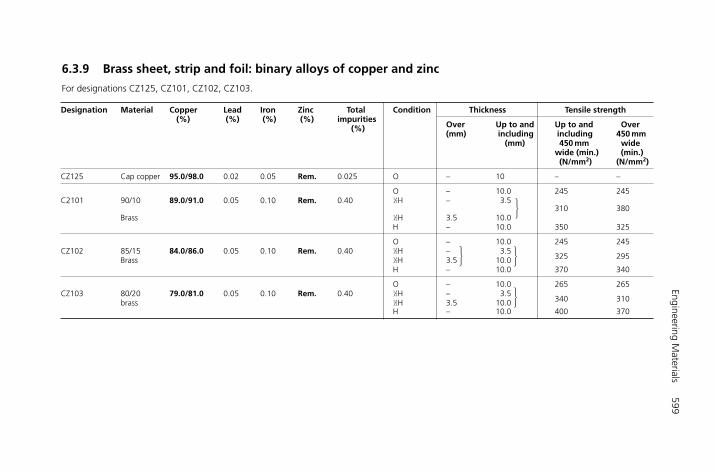
Engineering Materials
599
Designation Material Copper Lead Iron Zinc Total Condition Thickness Tensile strength(%) (%) (%) (%) impurities
Over Up to and Up to and Over (%)(mm) including including 450 mm
(mm) 450 mm wide wide (min.) (min.)(N/mm2) (N/mm2)
CZ125 Cap copper 95.0/98.0 0.02 0.05 Rem. 0.025 O – 10 – –
O – 10.0 245 245C2101 90/10 89.0/91.0 0.05 0.10 Rem. 0.40 1⁄2H – 3.5
310 380Brass 1⁄2H 3.5 10.0
H – 10.0 350 325
O – 10.0 245 245CZ102 85/15 84.0/86.0 0.05 0.10 Rem. 0.40 1⁄2H – 3.5
325 295Brass 1⁄2H 3.5 10.0H – 10.0 370 340
O – 10.0 265 265CZ103 80/20 79.0/81.0 0.05 0.10 Rem. 0.40 1⁄2H – 3.5
340 310brass 1⁄2H 3.5 10.0H – 10.0 400 370
6.3.9 Brass sheet, strip and foil: binary alloys of copper and zinc
For designations CZ125, CZ101, CZ102, CZ103.
�
�
�
�

600M
echanical Engineer’s Pocket Book
Elongation Vickers hardness (HV) Bend teston 50 mm
Up to and including Over 450 mm wide Transverse bend Longitudinal bend Complies min. (%)450 mm wide with or
falls within ISO
min. max. min. max. Angle Radius Angle Radius(degree) (degree)
CZ125 – – 75 – 75 180 Close 180 Close –
CZ101 35 – 75 – 75 180 Close 180 Close ISO 426/1
7 95 – 85 – 180 Close 180 Close Cu Zn 10180 t 180 t
3 110 – 100 – 90 2t 90 t
CZ102 35 – 75 – 75 180 Close 180 Close ISO 426/1180 Close 180 Close Cu Zn 15
7 95 – 85 – 180 t 180 t3 110 – 100 – 90 2t 90 t
CZ103 40 – 80 – 80 180 Close 180 Close ISO 426/1180 Close 180 Close Cu Zn 20
10 95 – 85 – 180 t 180 t5 120 – 110 – 90 2t 90 t
Further properties for the materials listed aboveD
esig
nat
ion
�
�
�
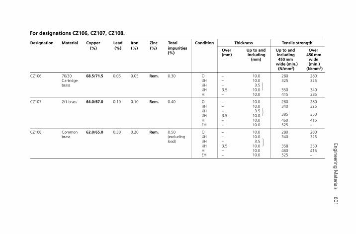
Engineering Materials
601
Designation Material Copper Lead Iron Zinc Total Condition Thickness Tensile strength(%) (%) (%) (%) impurities Over Up to and Up to and Over
(%) (mm) including including 450 mm (mm) 450 mm wide
wide (min.) (min.)(N/mm2) (N/mm2)
CZ106 70/30 68.5/71.5 0.05 0.05 Rem. 0.30 O – 10.0 280 280Cartridge 1⁄4H – 10.0 325 325brass 1⁄2H – 3.5
1⁄2H 3.5 10.0 350 340H – 10.0 415 385
CZ107 2/1 brass 64.0/67.0 0.10 0.10 Rem. 0.40 O – 10.0 280 2801⁄4H – 10.0 340 3251⁄2H – 3.51⁄2H 3.5 10.0 385 350
H – 10.0 460 415EH – 10.0 525 –
CZ108 Common 62.0/65.0 0.30 0.20 Rem. 0.50 O – 10.0 280 280brass (excluding 1⁄4H – 10.0 340 325
lead) 1⁄2H – 3.51⁄2H 3.5 10.0 358 350H – 10.0 460 415EH – 10.0 525 –
For designations CZ106, CZ107, CZ108.
�
�
�
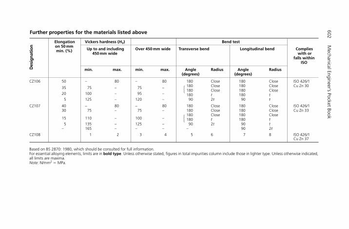
602M
echanical Engineer’s Pocket Book
Elongation Vickers hardness (HV) Bend teston 50 mm
Up to and including Over 450 mm wide Transverse bend Longitudinal bend Complies min. (%)450 mm wide with or
falls within ISO
min. max. min. max. Angle Radius Angle Radius(degrees) (degrees)
CZ106 50 – 80 – 80 180 Close 180 Close ISO 426/1
35 75 – 75 – 180 Close 180 Close Cu Zn 30180 Close 180 Close
20 100 – 95 – 180 t 180 t5 125 – 120 – 90 2t 90 t
CZ107 40 – 80 – 80 180 Close 180 Close ISO 426/130 75 – 75 – 180 Close 180 Close Cu Zn 33
15 110 – 100 –180 Close 180 Close180 t 180 t
5 135 – 125 – 90 2t 90 t– 165 – – – – 90 2t
CZ108 1 2 3 4 5 6 7 8 ISO 426/1 Cu Zn 37
Based on BS 2870: 1980, which should be consulted for full information.For essential alloying elements, limits are in bold type. Unless otherwise stated, figures in total impurities column include those in lighter type. Unless otherwise indicated,all limits are maxima.Note: N/mm2 � MPa.
Further properties for the materials listed aboveD
esig
nat
ion
�
�

Engineering Materials
603
Designation Material Copper Tin Lead Iron Zinc Aluminium Arsenic Total Condition Thickness (%) (%) (%) (%) (%) (%) (%) impurities up to and
(%) including (mm)
CZ110 Aluminium brass 76.0/78.0 – 0.04 0.06 Rem. 1.80/2.30 0.02/0.05 0.30 M 10.0O 10.0
CZ112 Naval brass 61.0/63.5 1.0/1.4 – – Rem. – – 0.75 M or O 10.0H 10.0
CZ118 Leaded brass 63.0/66.0 – 0.75/1.5 – Rem. – – 0.30 1⁄2H 6.064% Cu 1% Pb H 6.0
EH 6.0
CZ119 Leaded brass 61.0/64.0 – 1.0/2.5 – Rem. – – 0.30 1⁄2H 6.062% Cu 2% Pb H 6.0
EH 6.0
CZ120 Leaded brass 58.0/60.0 – 1.5/2.5 – Rem. – – 0.30 1⁄2H 6.059% Cu 2% Pb H 6.0
EH 6.0
CZ123 60/40 low lead 59.0/62.0 – 0.3/0.8 – Rem. – – 0.30 M 10.0brass: stamping brass
6.3.10 Brass sheet, strip and foil: special alloys and leaded brasses

604M
echanical Engineer’s Pocket Book
Tensile Elongation Vickers hardness Bend teststrength on 50 mm (HV)
Transverse bend Longitudinal bend(min.) (min.) (%)Complies with or(N/mm2)falls within ISO
min. max. Angle Radius Angle Radius(degrees) (degrees)
CZ110 340 45 – – – – – – ISO 462/2310 50 – 80 180 Close 180 Close Cu Zn 20/A12
CZ112 340 25 – – 180 t 180 t –400 20 – – – – 90 t
CZ118 370 10 110 140 – – – –430 5 140 165 – – – – –510 3 165 190 – – – –
CZ119 370 10 110 140 – – – –430 5 140 165 – – – – –510 3 165 190 – – – –
CZ120 – 10 110 140 – – – – ISO 426/2510 5 140 165 – – – – Cu Zn 39/Pb 2575 3 165 190 – – – –
CZ123 370 – 20 – – – – – ISO 426/2 Cu Zn 40/Pb
Based on BS 2870: 1980, which should be consulted for full information.For essential alloying elements, limits are in bold type. Unless otherwise stated, figures in total impurities column include those in lighter type. Unless otherwise indicated,all limits are maxima.Note: N/mm2 � MPa.
Des
ign
atio
nProperties for the materials listed above

Engineering Materials
605
Designation Material Copper Tin Lead Phosphorus Zinc Total Condition Thickness Tensile strength(%) (%) (%) (%) (%) impurities up to and
Up to and Over 450 mm(%) includingincluding wide min.(mm)450 mm (N/mm2)
wide min.
(N/mm2)
PB101 4% phosphor O 10.0 295 259bronze (copper– 1⁄4H 10.0 340 340tin–phosphorus) Rem. 3.5/4.5 0.2 0.02/0.40 0.30 0.50 1⁄2H 10.0 430 400
H 6.0 510 495EH 6.0 620 –
PB102 5% phosphor O 10.0 310 310bronze (copper– 1⁄4H 10.0 350 350tin–phosphorus) Rem. 4.5/5.5 0.02 0.02/0.40 0.30 0.50 1⁄2H 10.0 495 460
H 6.0 570 525EH 6.0 645 –SH 0.9 – –
PB103 7% phosphor O 10.0 340 340bronze (copper– 1⁄4H 10.0 385 385tin–phosphorus) 1⁄2H 10.0 525 460
Rem. 5.5/7.5 0.02 0.02/0.40 0.30 0.50 H 6.0 620 540EH 6.0 695 –SH 0.9 – –ESH 0.6 – –
6.3.11 Phosphor bronze sheet, strip and foil
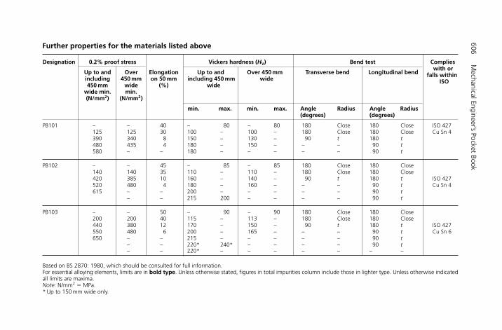
606M
echanical Engineer’s Pocket Book
Designation 0.2% proof stress Vickers hardness (HV) Bend test Complies
Up to and Over Elongation Up to and Over 450 mm Transverse bend Longitudinal bendwith or
including 450 mm on 50 mm including 450 mm widefalls within
450 mm wide (%) wideISO
wide min. min.(N/mm2) (N/mm2)
min. max. min. max. Angle Radius Angle Radius(degrees) (degrees)
PB101 – – 40 – 80 – 80 180 Close 180 Close ISO 427125 125 30 100 – 100 – 180 Close 180 Close Cu Sn 4390 340 8 150 – 130 – 90 t 180 t480 435 4 180 – 150 – – – 90 t580 – – 180 – – – – – 90 t
PB102 – – 45 – 85 – 85 180 Close 180 Close140 140 35 110 – 110 – 180 Close 180 Close420 385 10 160 – 140 – 90 t 180 t ISO 427520 480 4 180 – 160 – – – 90 t Cu Sn 4615 – – 200 – – – – – 90 t
– – 215 200 – – – – 90 t
PB103 – – 50 – 90 – 90 180 Close 180 Close200 200 40 115 – 113 – 180 Close 180 Close440 380 12 170 – 150 – 90 t 180 t ISO 427550 480 6 200 – 165 – – – 90 t Cu Sn 6650 – – 215 – – – – – 90 t
– – 220* 240* – – – – 90 t– – 220* – – – – – – –
Based on BS 2870: 1980, which should be consulted for full information.For essential alloying elements, limits are in bold type. Unless otherwise stated, figures in total impurities column include those in lighter type. Unless otherwise indicatedall limits are maxima.Note: N/mm2 � MPa.* Up to 150 mm wide only.
Further properties for the materials listed above

Engineering Materials 607
6.3.12 Aluminium bronze alloys – introduction
Despite their name, these are copper-based alloys containing up to 10% (nominal) alu-minium. They combine relatively high strength with excellent corrosion resistance at hightemperatures. These alloys can be grouped into two categories.
Single-phase alloysThe single phase, or �-alloys, contain up to 5% aluminium. They are highly ductile andcorrosion resistant. As the colour of the �-alloys resembles 18 carat gold, this alloy iswidely used in the manufacture of costume jewellery. This range of alloys are also widelyused in engineering, particularly for pipework where corrosion resistance at high temper-atures is required.
Duplex-phase alloysThese alloys contain approximately 10% aluminium and can be heat treated in a similarmanner to plain carbon steels. Heating followed by slow cooling anneals this alloy givinga primary �-phase (analogous to ferrite) in a eutectoid matrix of � � �2 (analogous topearlite). This results in the alloy becoming relatively soft and ductile. Heating followed byrapid cooling (quenching) produces a hard �� structure (analogous to martensite). Anexample of the composition and properties of a typical duplex-phase alloy is given in thefollowing table.
The duplex-phase alloys are also used for both sand- and die-casting where high strengthcombined with corrosion resistance and pressure tightness is required. However, thesealloys are not easy to cast as the aluminium content tends to oxidize at their relatively highmelting temperatures. Special precautions have to be taken to overcome this difficultyand these increase the cost of the process.
H6508-Ch06.3a.qxd 9/12/05 4:55 PM Page 607
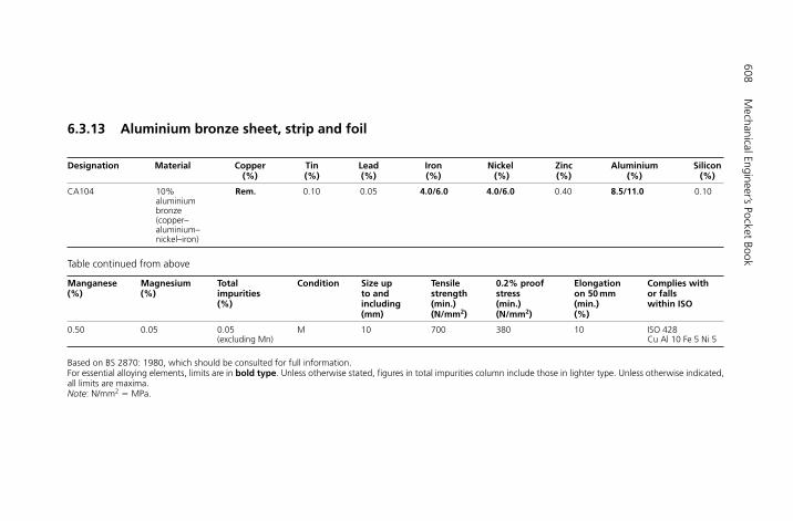
608M
echanical Engineer’s Pocket Book
6.3.13 Aluminium bronze sheet, strip and foil
Designation Material Copper Tin Lead Iron Nickel Zinc Aluminium Silicon (%) (%) (%) (%) (%) (%) (%) (%)
CA104 10% Rem. 0.10 0.05 4.0/6.0 4.0/6.0 0.40 8.5/11.0 0.10aluminium bronze (copper–aluminium–nickel–iron)
Table continued from above
Manganese Magnesium Total Condition Size up Tensile 0.2% proof Elongation Complies with(%) (%) impurities to and strength stress on 50 mm or falls
(%) including (min.) (min.) (min.) within ISO(mm) (N/mm2) (N/mm2) (%)
0.50 0.05 0.05 M 10 700 380 10 ISO 428 (excluding Mn) Cu Al 10 Fe 5 Ni 5
Based on BS 2870: 1980, which should be consulted for full information.For essential alloying elements, limits are in bold type. Unless otherwise stated, figures in total impurities column include those in lighter type. Unless otherwise indicated,all limits are maxima.Note: N/mm2 � MPa.
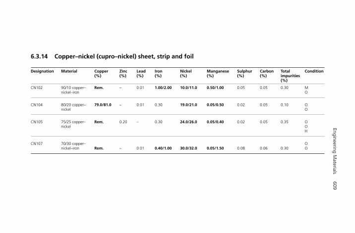
Engineering Materials
609
6.3.14 Copper–nickel (cupro–nickel) sheet, strip and foil
Designation Material Copper Zinc Lead Iron Nickel Manganese Sulphur Carbon Total Condition(%) (%) (%) (%) (%) (%) (%) (%) impurities
(%)
CN102 90/10 copper– Rem. – 0.01 1.00/2.00 10.0/11.0 0.50/1.00 0.05 0.05 0.30 Mnickel–iron O
CN104 80/20 copper– 79.0/81.0 – 0.01 0.30 19.0/21.0 0.05/0.50 0.02 0.05 0.10 Onickel O
CN105 75/25 copper– Rem. 0.20 – 0.30 24.0/26.0 0.05/0.40 0.02 0.05 0.35 Onickel O
H
CN107 70/30 copper– Onickel–iron Rem. – 0.01 0.40/1.00 30.0/32.0 0.05/1.50 0.08 0.06 0.30 O

610M
echanical Engineer’s Pocket Book
Designation Thickness Tensile Elongation Bend test: longitudinal Vickers Complies with strength on 50 mm and transverse bend hardness or falls within
min. (%) (HV) ISO(N/mm2)
Over Up to and Angle Radius(mm) including (degrees)
min. (mm)
CN102 – 10.0 310 30 – – 90 (max.) ISO 429– 10.0 280 40 – – Cu Ni 10 Fe 1 Mn
CN104 0.6 2.0 310 35 180 Close – ISO 4292.0 10.0 310 38 180 Close Cu Ni 20
CN105 0.6 2.0 340 30 180 Close – ISO 4292.0 10.0 340 35 180 Close – Cu Ni 250.6 10.0 – – – – 155 (min.)
CN107 0.6 2.0 370 30 180 Close ISO 4292.0 10.0 370 35 180 Close – Cu Ni 30 Mn 1 Fe
Based on BS 2870: 1980, which should be consulted for full information.For essential alloying elements, limits are in bold type. Unless otherwise stated, figures in total impurities column include those in lighter type. Unless otherwise indicated,all limits are maxima.Note: N/mm2 � MPa.
Table continued from above
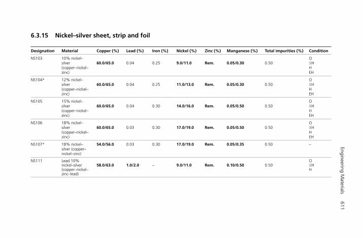
Engineering Materials
611
6.3.15 Nickel–silver sheet, strip and foil
Designation Material Copper (%) Lead (%) Iron (%) Nickel (%) Zinc (%) Manganese (%) Total impurities (%) Condition
NS103 10% nickel– Osilver 60.0/65.0 0.04 0.25 9.0/11.0 Rem. 0.05/0.30 0.50 1⁄2H(copper–nickel– Hzinc) EH
NS104* 12% nickel– Osilver 60.0/65.0 0.04 0.25 11.0/13.0 Rem. 0.05/0.30 0.50 1⁄2H(copper–nickel– Hzinc) EH
NS105 15% nickel– Osilver 60.0/65.0 0.04 0.30 14.0/16.0 Rem. 0.05/0.50 0.50 1⁄2H(copper–nickel– Hzinc) EH
NS106 18% nickel– Osilver 60.0/65.0 0.03 0.30 17.0/19.0 Rem. 0.05/0.50 0.50 1⁄2H(copper–nickel– Hzinc) EH
NS107* 18% nickel– 54.0/56.0 0.03 0.30 17.0/19.0 Rem. 0.05/0.35 0.50 –silver (copper–nickel–zinc)
NS111 Lead 10% Onickel–silver 58.0/63.0 1.0/2.0 – 9.0/11.0 Rem. 0.10/0.50 0.50 1⁄2H(copper–nickel– Hzinc–lead)

612M
echanical Engineer’s Pocket Book
Designation Bend test Vickers hardness (HV) Thickness up to Complies with or
Transverse bend Longitudinal bendand including falls within ISO
(mm)
Angle degrees Radius Angle degrees Radius min. max.
NS103 180 t 180 t – 100 10.0180 t 180 t 125 – 10.0 –90 t 90 t 160 – 10.0
– – 90 t 185 – 10.0
NS104* 180 t 180 t – 100 10.0180 t 180 t 130 – 10.090 t 90 t 160 – 10.0 –
– – 90 t 190 – 10.0
NS105 180 t 180 t – 105 10.0180 t 180 t 135 – 10.0 –90 t 90 t 165 – 10.0
– – 90 t 195 – 10.0
NS106 180 t 180 t – 110 10.0 ISO 430180 t 180 t 135 – 10.0 Cu Ni 18 Zn 2090 t 90 t 170 – 10.0
– – 90 t 200 – 10.0
NS107* – – – – – – – ISO 430 Cu Ni 18 Zn 27
NS111 – – – – – 100 –– – – – 150 180 – –– – – – 160 – –
Based on BS 2870: 1980, which should be consulted for full information.For essential alloying elements, limits are in bold type. Unless otherwise stated, figures in total impurities column include those in lighter type. Unless otherwise indicated,all limits are maxima.* For special requirements relevant to particular applications, see BS 2870: 1980, Section 4.
Table continued from above
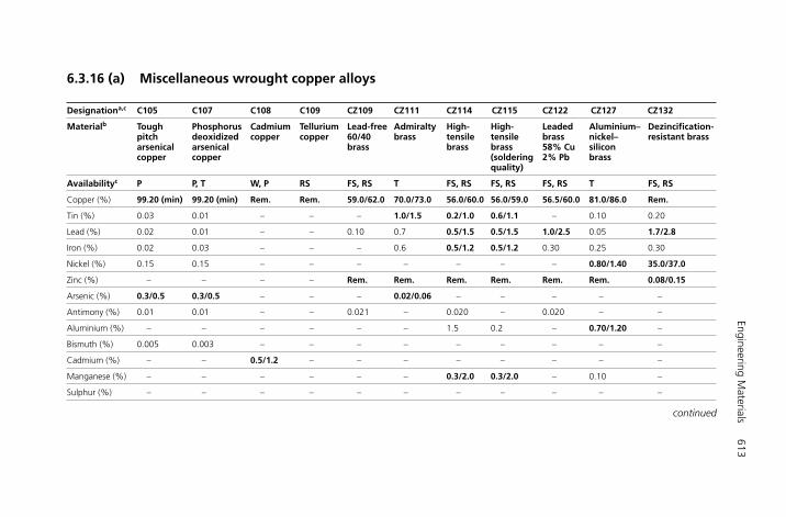
Engineering Materials
613
6.3.16 (a) Miscellaneous wrought copper alloys
Designationa,c C105 C107 C108 C109 CZ109 CZ111 CZ114 CZ115 CZ122 CZ127 CZ132
Materialb Tough Phosphorus Cadmium Tellurium Lead-free Admiralty High- High- Leaded Aluminium– Dezincification-pitch deoxidized copper copper 60/40 brass tensile tensile brass nickel– resistant brassarsenical arsenical brass brass brass 58% Cu silicon copper copper (soldering 2% Pb brass
quality)
Availabilityc P P, T W, P RS FS, RS T FS, RS FS, RS FS, RS T FS, RS
Copper (%) 99.20 (min) 99.20 (min) Rem. Rem. 59.0/62.0 70.0/73.0 56.0/60.0 56.0/59.0 56.5/60.0 81.0/86.0 Rem.
Tin (%) 0.03 0.01 – – – 1.0/1.5 0.2/1.0 0.6/1.1 – 0.10 0.20
Lead (%) 0.02 0.01 – – 0.10 0.7 0.5/1.5 0.5/1.5 1.0/2.5 0.05 1.7/2.8
Iron (%) 0.02 0.03 – – – 0.6 0.5/1.2 0.5/1.2 0.30 0.25 0.30
Nickel (%) 0.15 0.15 – – – – – – – 0.80/1.40 35.0/37.0
Zinc (%) – – – – Rem. Rem. Rem. Rem. Rem. Rem. 0.08/0.15
Arsenic (%) 0.3/0.5 0.3/0.5 – – – 0.02/0.06 – – – – –
Antimony (%) 0.01 0.01 – – 0.021 – 0.020 – 0.020 – –
Aluminium (%) – – – – – – 1.5 0.2 – 0.70/1.20 –
Bismuth (%) 0.005 0.003 – – – – – – – – –
Cadmium (%) – – 0.5/1.2 – – – – – – – –
Manganese (%) – – – – – – 0.3/2.0 0.3/2.0 – 0.10 –
Sulphur (%) – – – – – – – – – – –
continued

614M
echanical Engineer’s Pocket Book
Designationa,c C105 C107 C108 C109 CZ109 CZ111 CZ114 CZ115 CZ122 CZ127 CZ132
Materialb Tough Phosphorus Cadmium Tellurium Lead-free Admiralty High- High- Leaded Aluminium– Dezincification-pitch deoxidized copper copper 60/40 brass tensile tensile brass nickel– resistant brassarsenical arsenical brass brass brass 58% Cu silicon copper copper (soldering 2% Pb brass
quality)
Availabilityc P P, T W, P RS FS, RS T FS, RS FS, RS FS, RS T FS, RS
Silicon (%) – – – – – – – – – 0.80/1.30 –
Oxygen (%) 0.70 – – – – – – – – – –
Phosphorus (%) – 0.013/0.050 – – – – – – – – –
Tellurium (%) Se � Te 0.010 – 0.3/0.7 – – – – – – –0.03 Se � Te
0.20
Total – 0.07 0.05 – 0.30 0.30 0.50 0.50 0.75 0.50 0.60impurities (%) (excluding (excluding (excluding
silver, arsenic, lead) tin, lead,nickel, iron, phosphorus) manganese)
For essential alloying elements, limits are in bold type. Unless otherwise stated, figures in total impurities column include those in lighter type. Unless otherwise indicated,all limits are maxima.aThese alloys are not included in BS 2870, except in Appendix A of that standard, but are available in other product forms and other BS specifications.bOxygen-free high-conductivity copper for special applications (C110) is found in BS 1433, BS 1977, BS 3839 and BS 4608. This material is used for conductors in elec-trical and electronic applications.cAvailability: T � tube, FS � forging stock, W � wire, RS � rods, sections, P � plate.
Section 6.3.16(a) (continued)
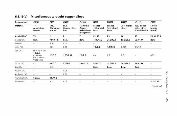
Engineering Materials
615
6.3.16(b) Miscellaneous wrought copper alloys
Designationa CA102 C105 CN101 CN108 NS101 NS102 NS109 NS112 CS101
Material 7% 10% 95/5 66/30/2/2 Leaded Leaded 25% nickel– 15% leaded Silicon–Aluminium– Aluminium– Copper–nickel– Copper– 10% nickel– 14% nickel– silver nickel–silver bronzebronze bronze iron nickel–iron– brass brass (Cu–Ni–Zn–Pb) (Cu–Si)
manganese
Availabilityb T, P P P T FS, RS RS W RS FS, W, RS, P
Copper (%) Rem. 78.0/85.0 Rem. Rem. 44.0/47.0 34.0/42.0 55.0/60.0 60.0/63.0 Rem.
Tin (%) – 0.10 0.01 – – – – – –
Lead (%) – 0.05 0.01 – 1.0/2.5 1.0/2.25 0.025 0.5/1.0 –
Iron (%) Ni � Fe � Mn1.0/2.5 (optional) 1.5/3.5 1.05/1.35 1.7/2.3 0.4 0.3 0.3 – 0.25but betweenthese limits
Nickel (%) – 4.0/7.0 5.0/6.0 29.0/32.0 9.0/11.0 13.0/15.0 24.0/26.0 14.0/16.0 –
Zinc (%) – 0.40 – – Rem. Rem. Rem. Rem. –
Arsenic (%) – – 0.05 – – – – – –
Antimony (%) – – 0.01 – – – – – –
Aluminium (%) 6.0/7.5 8.5/10.5 – – – – – – –
Silicon (%) – 0.15 0.05 – – – – – 3.15/3.25
continued
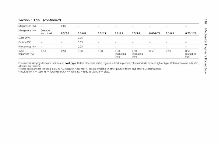
616M
echanical Engineer’s Pocket Book
Section 6.3.16 (continued)
Magnesium (%) – 0.05 – – – – – – –
Manganese (%) See iron and nickel 0.5/2.0 0.3/0.8 1.5/2.5 0.2/0.5 1.5/3.0 0.05/0.75 0.1/0.5 0.75/1.25
Sulphur (%) – – 0.05 – – – – – –
Carbon (%) – – 0.05 – – – – – –
Phosphorus (%) – – 0.03 – – – – – –
Total 0.50 0.50 0.30 0.30 0.30 0.30 0.50 0.50 0.50 impurities (%) (excluding (excluding (excluding
iron) iron) iron)
For essential alloying elements, limits are in bold type. Unless otherwise stated, figures in total impurities column include those in lighter type. Unless otherwise indicated,all limits are maxima.a These alloys are not included in BS 2870, except in Appendix A, but are available in other product forms and other BS specifications.b Availability: T � tube, FS � forging stock, W � wire, RS � rods, sections, P � plate.

Engineering Materials
617
6.3.17(a) Copper alloys for casting: group A
Designation PB4 LPB1 LB2 LB4 LG1 LG2
Material Phosphor Leaded Leaded Leaded Leaded Leaded bronze phosphor bronze bronze gunmetal gunmetal
(copper–tin– bronzephosphorus)
Nominal Cu Sn 10 Pb P Cu Sn 7 Pb P Cu Sn 10 Pb 10 Cu Sn 5 Pb 9 Cu Sn 3 Pb 5 Zn 8 Cu Sn 5 Pb 5 Zn 5composition
Elements min. max. min. max. min. max. min. max. min. max. min. max.(%) (%) (%) (%) (%) (%) (%) (%) (%) (%) (%) (%)
Copper Remainder Remainder Remainder Remainder Remainder RemainderTin 9.5 11.0 6.5 8.5 9.0 11.0 4.0 6.0 2.0 3.5 4.0 6.0Zinc – 0.5 – 2.0 – 1.0 – 2.0 7.0 9.5 4.0 6.0
Lead – 0.75 2.0 5.0 8.5 11.0 8.0 10.0 4.0 6.0 4.0 6.0Phosphorus 0.4 1.0 0.33 – – 0.1 – 0.1a – – – –Nickel – 0.5 – 1.0 – 2.0 – 2.0 – 2.0 – 2.0
Iron – – – – – 0.15 – 0.25 – – – –Aluminium – – – – – 0.01 – 0.01 – 0.01 – 0.01Manganese – – – – – 0.20 – 0.20 – – – –
Antimony – – – 0.25 – 0.5 – 0.5 – – – –Arsenic – – – – – – – – – – – –Iron � arsenic � – – – – – – – – – 0.75 – 0.5antimony
Silicon – – – – – 0.02 – 0.02 – 0.02 – 0.02Bismuth – – – – – – – – – 0.10 – 0.05Sulphur – 0.1 – 0.1 – 0.1 – 0.1 – 0.10 – –
Total impurities – 0.5 – 0.5 – 0.5 – 0.5 – 1.0 – 0.80
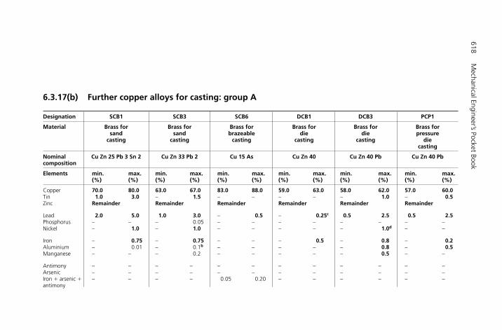
618M
echanical Engineer’s Pocket Book
Designation SCB1 SCB3 SCB6 DCB1 DCB3 PCP1
Material Brass for Brass for Brass for Brass for Brass for Brass forsand sand brazeable die die pressure
casting casting casting casting casting diecasting
Nominal Cu Zn 25 Pb 3 Sn 2 Cu Zn 33 Pb 2 Cu 15 As Cu Zn 40 Cu Zn 40 Pb Cu Zn 40 Pbcomposition
Elements min. max. min. max. min. max. min. max. min. max. min. max.(%) (%) (%) (%) (%) (%) (%) (%) (%) (%) (%) (%)
Copper 70.0 80.0 63.0 67.0 83.0 88.0 59.0 63.0 58.0 62.0 57.0 60.0Tin 1.0 3.0 – 1.5 – – – – – 1.0 – 0.5Zinc Remainder Remainder Remainder Remainder Remainder Remainder
Lead 2.0 5.0 1.0 3.0 – 0.5 – 0.25c 0.5 2.5 0.5 2.5Phosphorus – – – 0.05 – – – – – – – –Nickel – 1.0 – 1.0 – – – – – 1.0d – –
Iron – 0.75 – 0.75 – – – 0.5 – 0.8 – 0.2Aluminium – 0.01 – 0.1b – – – – – 0.8 – 0.5Manganese – – – 0.2 – – – – – 0.5 – –
Antimony – – – – – – – – – – – –Arsenic – – – – – – – – – – – –Iron � arsenic � – – – – 0.05 0.20 – – – – – –antimony
6.3.17(b) Further copper alloys for casting: group A

Engineering Materials
619
Silicon – – – 0.05 – – – – – 0.05 – –Bismuth – – – – – – – – – – – –Sulphur – – – – – – – – – – – –
Total – 1.0 – 1.0 – 1.0 – 0.75 – 2.0 – 0.5impurities (including (excluding
lead) Ni � Pb � Al)
For full range of alloys and further information, see BS 1400.For essential alloying elements, limits are in bold type. Unless otherwise stated, figures in total impurities column include those in lighter type. Unless otherwise indicated,all limits are maxima.aFor continuous casting, phosphorus content may be increased to a maximum of 1.5% and alloy coded with suffix /L.bFor pressure tight castings in SCB3 the aluminium content should not be greater than 0.02.cDCB1: 0.1% lead if required.dDCB3: nickel to be counted as copper.
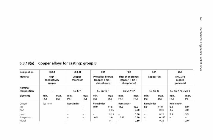
620M
echanical Engineer’s Pocket Book
Designation HCC1 CC1-TF PB1 PB2 CT1 LG4
Material High- Copper– Phosphor bronze Phosphor bronze Copper–tin 87/7/3/3conductivity chromium (copper � tin � (copper � tin � Leaded
copper phosphorus) phosphorus) gunmetal
Nominalcomposition – Cu Cr 1 Cu Sn 10 P Cu Sn 11 P Cu Sn 10 Cu Sn 7 PB 3 Zn 3
Elements min. max. min. max. min. max. min. max. min. max. min. max.(%) (%) (%) (%) (%) (%) (%) (%) (%) (%) (%) (%)
Copper See notea Remainder Remainder Remainder Remainder RemainderTin – – 10.0 11.5 11.0 13.0 9.0 11.0 6.0 8.0c
Zinc – – – 0.05 – 0.30 – 0.03 1.5 3.0
Lead – – – 0.25 – 0.50 – 0.25 2.5 3.5Phosphorus – – 0.5 1.0 0.15 0.60 – 0.15b – –Nickel – – – 0.1 – 0.50 – 0.25 – 2.0c
6.3.18(a) Copper alloys for casting: group B
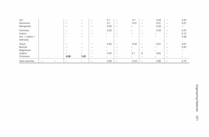
Engineering Materials
621
Iron – – – 0.1 – 0.1 – 0.20 – 0.20Aluminium – – – 0.1 – 0.01 – 0.01 – 0.01Manganese – – – 0.05 – – – 0.20 – –
Antimony – – – 0.05 – – – 0.20 – 0.25Arsenic – – – – – – – – – 0.15Iron � arsenic � – – – – – – – – – 0.40antimony
Silicon – – – 0.02 – 0.02 – 0.01 – 0.01Bismuth – – – – – – – – – 0.05Magnesium – – – – – – – – – –Sulphur – – – 0.05 – 0.1 0 0.05 – –Chromium 0.50 1.25 – – – – – – – –
Total impurities – – – – – 0.60 – 0.20 – 0.80 – 0.70
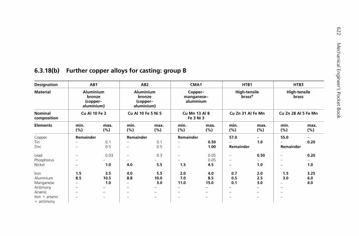
622M
echanical Engineer’s Pocket Book
Designation AB1 AB2 CMA1 HTB1 HTB3
Material Aluminium Aluminium Copper– High-tensile High-tensile bronze bronze manganese– brassd brass
(copper– (copper– aluminiumaluminium) aluminium)
Nominal Cu Al 10 Fe 3 Cu Al 10 Fe 5 Ni 5 Cu Mn 13 Al 8 Cu Zn 31 Al Fe Mn Cu Zn 28 Al 5 Fe Mncomposition Fe 3 Ni 3
Elements min. max. min. max. min. max. min. max. min. max.(%) (%) (%) (%) (%) (%) (%) (%) (%) (%)
Copper Remainder Remainder Remainder 57.0 – 55.0 –Tin – 0.1 – 0.1 – 0.50 – 1.0 – 0.20Zinc – 0.5 – 0.5 – 1.00 Remainder Remainder
Lead – 0.03 – 0.3 – 0.05 – 0.50 – 0.20Phosphorus – – – – – 0.05 – – – –Nickel – 1.0 4.0 5.5 1.5 4.5 – 1.0 – 1.0
Iron 1.5 3.5 4.0 5.5 2.0 4.0 0.7 2.0 1.5 3.25Aluminium 8.5 10.5 8.8 10.0 7.0 8.5 0.5 2.5 3.0 6.0Manganese – 1.0 – 3.0 11.0 15.0 0.1 3.0 – 4.0Antimony – – – – – – – – –Arsenic – – – – – – – – –Iron � arsenic – – – – – – – – –� antimony
6.3.18(b) Further copper alloys for casting: group B
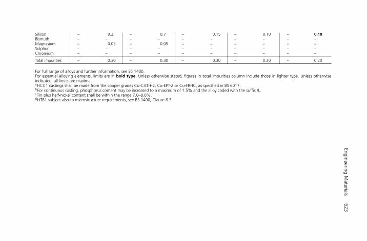
Engineering Materials
623
Silicon – 0.2 – 0.7 – 0.15 – 0.10 – 0.10Bismuth – – – – – – – – – –Magnesium – 0.05 – 0.05 – – – – – –Sulphur – – – – – – – – – –Chromium – – – – – – – – – –
Total impurities – 0.30 – 0.30 – 0.30 – 0.20 – 0.20
For full range of alloys and further information, see BS 1400.For essential alloying elements, limits are in bold type. Unless otherwise stated, figures in total impurities column include those in lighter type. Unless otherwise indicated, all limits are maxima.aHCC1 castings shall be made from the copper grades Cu-CATH-2, Cu-EPT-2 or Cu-FRHC, as specified in BS 6017.bFor continuous casting, phosphorus content may be increased to a maximum of 1.5% and the alloy coded with the suffix /L.cTin plus half-nickel content shall be within the range 7.0–8.0%.dHTB1 subject also to microstructure requirements, see BS 1400, Clause 6.3.
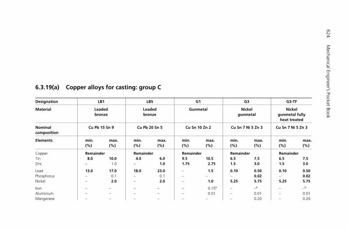
624M
echanical Engineer’s Pocket Book
Designation LB1 LB5 G1 G3 G3-TF
Material Leaded Leaded Gunmetal Nickel Nickel bronze bronze gunmetal gunmetal fully
heat treated
Nominal Cu Pb 15 Sn 9 Cu Pb 20 Sn 5 Cu Sn 10 Zn 2 Cu Sn 7 Ni 5 Zn 3 Cu Sn 7 Ni 5 Zn 3composition
Elements min. max. min. max. min. max. min. max. min. max.(%) (%) (%) (%) (%) (%) (%) (%) (%) (%)
Copper Remainder Remainder Remainder Remainder RemainderTin 8.0 10.0 4.0 6.0 9.5 10.5 6.5 7.5 6.5 7.5Zinc – 1.0 – 1.0 1.75 2.75 1.5 3.0 1.5 3.0
Lead 13.0 17.0 18.0 23.0 – 1.5 0.10 0.50 0.10 0.50Phosphorus – 0.1 – 0.1 – – – 0.02 – 0.02Nickel – 2.0 – 2.0 – 1.0 5.25 5.75 5.25 5.75
Iron – – – – – 0.15b – –b – –b
Aluminium – – – – – 0.01 – 0.01 – 0.01Manganese – – – – – – – 0.20 – 0.20
6.3.19(a) Copper alloys for casting: group C
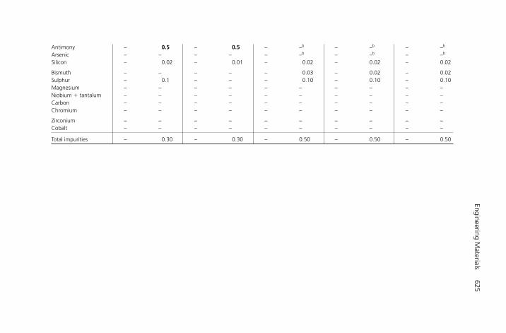
Engineering Materials
625
Antimony – 0.5 – 0.5 – –b – –b – –b
Arsenic – – – – – –b – –b – –b
Silicon – 0.02 – 0.01 – 0.02 – 0.02 – 0.02
Bismuth – – – – – 0.03 – 0.02 – 0.02Sulphur – 0.1 – – – 0.10 – 0.10 – 0.10Magnesium – – – – – – – – – –Niobium � tantalum – – – – – – – – – –Carbon – – – – – – – – – –Chromium – – – – – – – – – –
Zirconium – – – – – – – – – –Cobalt – – – – – – – – – –
Total impurities – 0.30 – 0.30 – 0.50 – 0.50 – 0.50
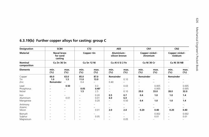
626M
echanical Engineer’s Pocket Book
Designation SCB4 CT2 AB3 CN1 CN2
Material Naval brass Copper–tin Aluminium– Copper–nickel– Copper–nickel–for sand silicon bronze chromium niobiumcasting
Nominal Cu Zn 36 Sn Cu Sn 12 Ni Cu Al 6 Si 2 Fe Cu Ni 30 Cr Cu Ni 30 NBcomposition
Elements min. max. min. max. min. max. min. max. min. max.(%) (%) (%) (%) (%) (%) (%) (%) (%) (%)
Copper 60.0 63.0 85.0 87.0 Remainder Remainder RemainderTin 1.0 1.5 11.0 13.0 – 0.10 – – – –Zinc Remainder – 0.4 – 0.40 – – – – –
Lead – 0.50 – 0.3 – 0.03 – 0.005 – 0.005Phosphorus – – 0.05 0.40a – – – 0.005 – 0.005Nickel – – 1.5 2.5 – 0.10 29.0 33.0 28.0 32.0
Iron – – – 0.20 0.5 0.7 0.4 1.0 1.0 1.4Aluminium – 0.01 – 0.01 6.0 6.4 – – – –Manganese – – – 0.20 – 0.50 0.4 1.0 1.0 1.4
Antimony – – – – – – – – – –.Arsenic – – – – – – – – – –Silicon – – – 0.01 2.0 2.4 0.20 0.40 0.20 0.40
Bismuth – – – – – – – 0.002 – 0.002Sulphur – – – 0.05 – – – 0.01 – 0.01Magnesium – – – – – 0.05 – – – –
6.3.19(b) Further copper alloys for casting: group C
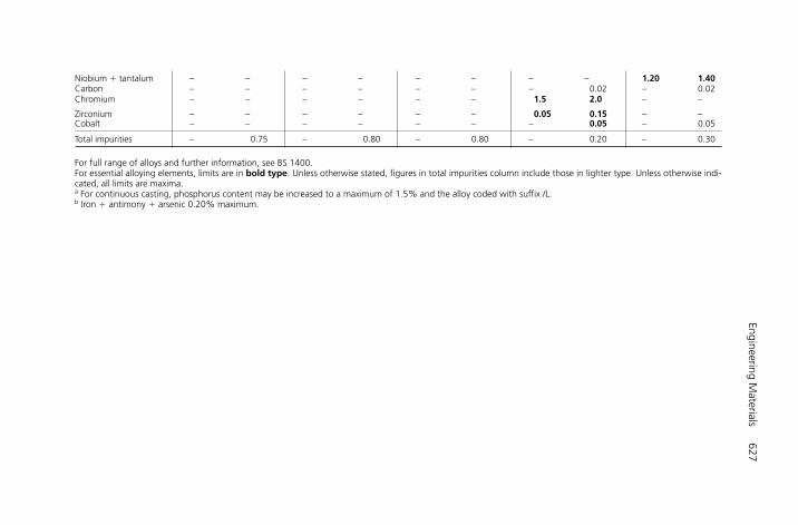
Engineering Materials
627
Niobium � tantalum – – – – – – – – 1.20 1.40Carbon – – – – – – – 0.02 – 0.02Chromium – – – – – – 1.5 2.0 – –
Zirconium – – – – – – 0.05 0.15 – –Cobalt – – – – – – – 0.05 – 0.05
Total impurities – 0.75 – 0.80 – 0.80 – 0.20 – 0.30
For full range of alloys and further information, see BS 1400.For essential alloying elements, limits are in bold type. Unless otherwise stated, figures in total impurities column include those in lighter type. Unless otherwise indi-cated, all limits are maxima.a For continuous casting, phosphorus content may be increased to a maximum of 1.5% and the alloy coded with suffix /L.b Iron � antimony � arsenic 0.20% maximum.
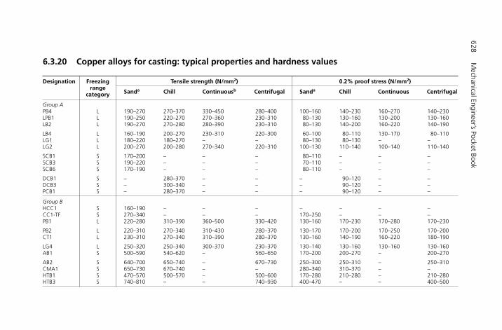
628M
echanical Engineer’s Pocket Book
Designation Freezing Tensile strength (N/mm2) 0.2% proof stress (N/mm2)range
Sanda Chill Continuousb Centrifugal Sanda Chill Continuous Centrifugalcategory
Group APB4 L 190–270 270–370 330–450 280–400 100–160 140–230 160–270 140–230LPB1 L 190–250 220–270 270–360 230–310 80–130 130–160 130–200 130–160LB2 L 190–270 270–280 280–390 230–310 80–130 140–200 160–220 140–190
LB4 L 160–190 200–270 230–310 220–300 60–100 80–110 130–170 80–110LG1 L 180–220 180–270 – – 80–130 80–130 – –LG2 L 200–270 200–280 270–340 220–310 100–130 110–140 100–140 110–140
SCB1 S 170–200 – – – 80–110 – – –SCB3 S 190–220 – – – 70–110 – – –SCB6 S 170–190 – – – 80–110 – – –
DCB1 S – 280–370 – – – 90–120 – –DCB3 S – 300–340 – – – 90–120 – –PCB1 S – 280–370 – – – 90–120 – –
Group BHCC1 S 160–190 – – – – – – –CC1-TF S 270–340 – – – 170–250 – – –PB1 L 220–280 310–390 360–500 330–420 130–160 170–230 170–280 170–230
PB2 L 220–310 270–340 310–430 280–370 130–170 170–200 170–250 170–200CT1 L 230–310 270–340 310–390 280–370 130–160 140–190 160–220 180–190
LG4 L 250–320 250–340 300–370 230–370 130–140 130–160 130–160 130–160AB1 S 500–590 540–620 – 560–650 170–200 200–270 – 200–270
AB2 S 640–700 650–740 – 670–730 250–300 250–310 – 250–310CMA1 S 650–730 670–740 – – 280–340 310–370 – –HTB1 S 470–570 500–570 – 500–600 170–280 210–280 – 210–280HTB3 S 740–810 – – 740–930 400–470 – – 400–500
6.3.20 Copper alloys for casting: typical properties and hardness values

Engineering Materials
629
Group CLB1 L 170–230 200–270 230–310 220–300 80–110 130–160 130–190 130–160LB5 L 160–190 170–230 190–270 190–270 60–100 80–110 100–160 80–110
G1 L 270–340 230–310 300–370 250–340 130–160 130–170 140–190 130–170G3 L 280–340 – 340–370 – 140–160 – 170–190 –G3-TF L 430–480 – 430–500 – 280–310 – 280–310 –
SCB4 S 250–310 – – – 70–110 – – –CT2 L 280–330 – 300–350 300–350 160–180 – 180–210 180–210AB3 S 460–500 – – – 180–190 – – –
CN1 S 480–540 – – – 300–320 – – –CN2 S 480–540 – – – 300–320 – – –
continued
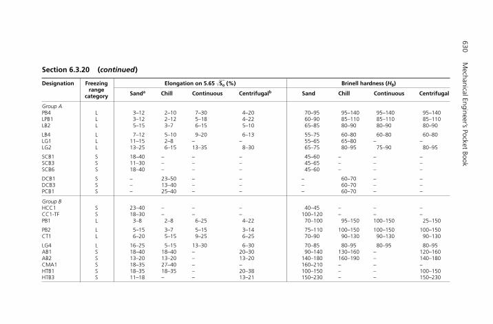
630M
echanical Engineer’s Pocket Book
Designation Freezing Elongation on 5.65 �__So (%) Brinell hardness (HB)
rangeSanda Chill Continuous Centrifugalb Sand Chill Continuous Centrifugalcategory
Group APB4 L 3–12 2–10 7–30 4–20 70–95 95–140 95–140 95–140LPB1 L 3–12 2–12 5–18 4–22 60–90 85–110 85–110 85–110LB2 L 5–15 3–7 6–15 5–10 65–85 80–90 80–90 80–90
LB4 L 7–12 5–10 9–20 6–13 55–75 60–80 60–80 60–80LG1 L 11–15 2–8 – – 55–65 65–80 – –LG2 L 13–25 6–15 13–35 8–30 65–75 80–95 75–90 80–95
SCB1 S 18–40 – – – 45–60 – – –SCB3 S 11–30 – – – 45–65 – – –SCB6 S 18–40 – – – 45–60 – – –
DCB1 S – 23–50 – – – 60–70 – –DCB3 S – 13–40 – – – 60–70 – –PCB1 S – 25–40 – – – 60–70 – –
Group BHCC1 S 23–40 – – – 40–45 – – –CC1-TF S 18–30 – – – 100–120 – – –PB1 L 3–8 2–8 6–25 4–22 70–100 95–150 100–150 25–150
PB2 L 5–15 3–7 5–15 3–14 75–110 100–150 100–150 100–150CT1 L 6–20 5–15 9–25 6–25 70–90 90–130 90–130 90–130
LG4 L 16–25 5–15 13–30 6–30 70–85 80–95 80–95 80–95AB1 S 18–40 18–40 – 20–30 90–140 130–160 – 120–160AB2 S 13–20 13–20 – 13–20 140–180 160–190 – 140–180CMA1 S 18–35 27–40 – – 160–210 – – –HTB1 S 18–35 18–35 – 20–38 100–150 – – 100–150HTB3 S 11–18 – – 13–21 150–230 – – 150–230
Section 6.3.20 (continued)

Engineering Materials
631
Group CLB1 L 4–10 3–7 9–10 4–10 50–70 70–90 70–90 70–90LB5 L 5–10 5–12 8–16 7–15 45–65 50–70 50–70 50–70
G1 L 13–25 3–8 9–25 5–16 70–95 85–130 90–130 70–95G3 L 16–25 – 18–25 – 70–95 – 90–130 –G3-TF L 3–5 – 3–7 – 160–180 – 160–180 –
SCB4 S 18–40 – – – 50–75 – – –CT2 L 12–20 – 8–15 10–15 75–110 – 100–150 100–150AB3 S 20–30 – – – – – – –
CN1 S 18–25 – – – 170–200 – – –CN2 S 18–25 – – – 170–200 – – –
aOn separately cast test bars.bValues apply to samples cut from centrifugal castings made in metallic moulds. Minimum properties of centrifugal castings made in sand moulds are the same as for sandcastings.

632 Mechanical Engineer’s Pocket Book
6.3.21 Aluminium and aluminium alloys
Pure aluminium has a low mechanical strength and is usually alloyed with other metals toproduce a wide range of useful, lightweight materials. The aluminium alloys can be dividedup into four categories:
● Wrought alloys that can be heat treated.● Wrought alloys that cannot be heat treated.● Cast alloys that can be heat treated.● Cast alloys that cannot be heat treated.
Like most non-ferrous metals and their alloys, aluminium and aluminium alloys depend oncold-working processes such as rolling and drawing to enhance their properties. Only a relatively few aluminium alloys containing copper and other alloying elements respondto heat treatment. An example of a general-purpose light-alloy originally developed for highly stressed aircraft components is duralumin. This alloy has the following composition:
Copper (Cu) 4.0%Silicon (Si) 0.2%Manganese (Mn) 0.7%Magnesium (Mg) 0.8%Aluminium (Al) Remainder
It can be softened by heating the alloy to 480°C and quenching this is known as solutiontreatment since the alloying elements form a solid solution with the aluminium renderingthe metal ductile and suitable for cold working without cracking. However, it starts to re-harden immediately by a natural process called age hardening and becomes fully hard-ened only after 4 days. During age hardening the unstable supersaturated solution of thealloying elements breaks down with the precipitation of the intermetallic compoundCuAl2. The precipitate will be in the form of fine particles throughout the mass of themetal to give greater strength and hardness.
Another alloy that is even stronger has the following composition:
Copper (Cu 1.6%Titanium (Ti) 0.3%Magnesium (Mg) 2.5%Zinc (Zn) 0.2%Aluminium (Al) Remainder
This alloy can also be softened by solution treatment by heating it to 465°C and quench-ing. Again hardening occurs by natural ageing. If the natural ageing process is speededup by reheating the alloy to 165°C for about 10 h, the process is called precipitation agehardening or artificial ageing. The age-hardening process can be retarded after solutiontreatment by refrigeration.
6.3.22 British Standards
Some useful British Standards relating to wrought and cast aluminium and aluminiumalloys – both heat-treatable and non-heat-treatable are as follows:
● BS EN 485-2: 2004 Aluminium and Aluminium alloys – sheet, strip and plate – chemicalcomposition.
● BS EN 485-2: 2004 Aluminium and aluminium alloys – sheet, strip and plate – mechanicalproperties.
H6508-Ch06.3b.qxd 9/21/05 4:32 PM Page 632

● BS EN 573: 1995 (four parts) – wrought products:(a) Part 1: Numerical designation system.(b) Part 2: Chemical symbol-based designation system.(c) Part 3: Chemical composition.(d) Part 4: Forms of products.
● BS EN 1559-4: 1999 Founding – additional requirements for aluminium and alu-minium alloy castings.
● BS 1706: 1998 Aluminium and aluminium alloy castings – chemical composition andmechanical properties.
These are highly detailed and comprehensive standards, and it is not physically possible toreproduce them within the confines of this Pocket Book. However, they should be con-sulted when selecting materials for a new product design and manufacture.
Some typical examples of wrought and cast aluminium and aluminium alloy products arelisted in tables in the following sections. They are for guidance only.
Engineering Materials 633
H6508-Ch06.3b.qxd 9/21/05 4:32 PM Page 633
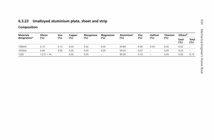
634M
echanical Engineer’s Pocket Book
6.3.23 Unalloyed aluminium plate, sheet and strip
Composition
Materials Silicon Iron Copper Manganese Magnesium Aluminiumc Zinc Gallium Titanium Othersb
designationa (%) (%) (%) (%) (%) (%) (%) (%) (%)Each Total(%) (%)
1080(A) 0.15 0.15 0.03 0.02 0.02 99.80 0.06 0.03 0.02 0.02 –
1050(A) 0.40 0.05 0.05 0.05 0.05 99.50 0.07 – 0.05 0.03 –
1200 1.0 Si � Fe 0.05 0.05 – 99.00 0.10 – 0.05 0.05 0.15
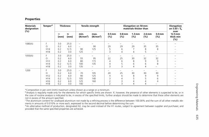
Engineering Materials
635
Properties
Materials Temperd Thickness Tensile strength Elongation on 50 mm: Elongation designation materials thicker than on 5.65���So(%) over
� � min. max. 0.5 mm 0.8 mm 1.3 mm 2.6 mm 3.0 mm 12.5 mm (mm) (mm) (N/mm2) (N/mm2) (%) (%) (%) (%) (%) thick min
(%)
1080(A) F 3.0 25.0 – – – – – – – –O 0.2 6.0 – 90 29 29 29 35 35 –H14 0.2 12.5 90 125 5 6 7 8 8 –H18 0.2 3.0 125 – 3 4 4 5 – –
1050(A) F 3.0 25.0 – – – – – – – –O 0.2 6.0 55 95 22 25 30 32 32 –H12 0.2 6.0 80 115 4 6 8 9 9 –H14 0.2 12.5 100 135 4 5 6 6 8 –H18 0.2 3.0 135 – 3 3 4 4 – –
1200 F 3.0 25.0 – – – – – – – –O 0.2 6.0 70 105 20 25 30 30 30 –H12 0.2 6.0 90 125 4 6 8 9 9 –H14 0.2 12.5 105 140 3 4 5 5 6 –H16 0.2 6.0 125 160 2 3 4 4 4 –H18 0.2 3.0 140 – 2 3 4 4 – –
aComposition in per cent (m/m) maximum unless shown as a range or a minimum.bAnalysis is regularly made only for the elements for which specific limits are shown. If, however, the presence of other elements is suspected to be, or inthe case of routine analysis is indicated to be, in excess of the specified limits, further analysis should be made to determine that these other elements arenot in excess of the amount specified.cThe aluminium content for unalloyed aluminium not made by a refining process is the difference between 100.00% and the sum of all other metallic ele-ments in amounts of 0.010% or more each, expressed to the second decimal before determining the sum.dAn alternative method of production, designated H2, may be used instead of the H1 routes, subject to agreement between supplier and purchaser, andprovided that the same specified properties are achieved.
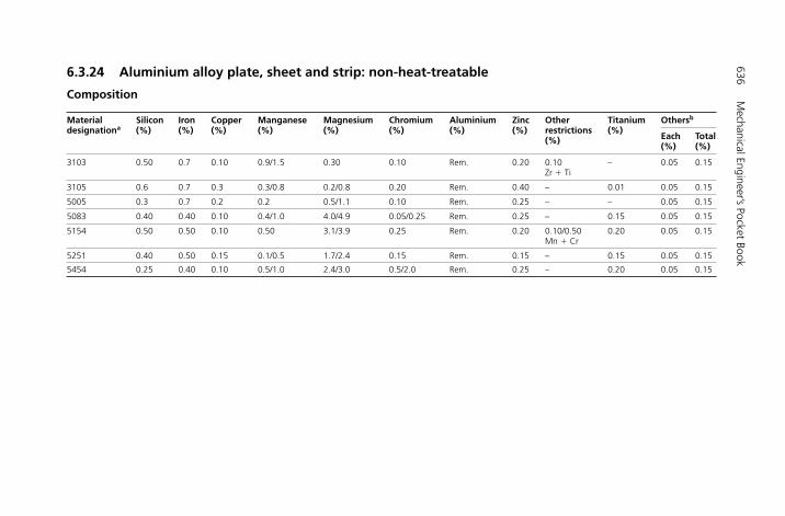
636M
echanical Engineer’s Pocket Book
6.3.24 Aluminium alloy plate, sheet and strip: non-heat-treatable
Composition
Material Silicon Iron Copper Manganese Magnesium Chromium Aluminium Zinc Other Titanium Othersb
designationa (%) (%) (%) (%) (%) (%) (%) (%) restrictions (%)Each Total(%)(%) (%)
3103 0.50 0.7 0.10 0.9/1.5 0.30 0.10 Rem. 0.20 0.10 – 0.05 0.15Zr � Ti
3105 0.6 0.7 0.3 0.3/0.8 0.2/0.8 0.20 Rem. 0.40 – 0.01 0.05 0.15
5005 0.3 0.7 0.2 0.2 0.5/1.1 0.10 Rem. 0.25 – – 0.05 0.15
5083 0.40 0.40 0.10 0.4/1.0 4.0/4.9 0.05/0.25 Rem. 0.25 – 0.15 0.05 0.15
5154 0.50 0.50 0.10 0.50 3.1/3.9 0.25 Rem. 0.20 0.10/0.50 0.20 0.05 0.15Mn � Cr
5251 0.40 0.50 0.15 0.1/0.5 1.7/2.4 0.15 Rem. 0.15 – 0.15 0.05 0.15
5454 0.25 0.40 0.10 0.5/1.0 2.4/3.0 0.5/2.0 Rem. 0.25 – 0.20 0.05 0.15
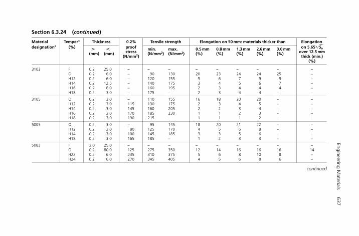
Engineering Materials
637
Material Temperc Thickness 0.2% Tensile strength Elongation on 50 mm: materials thicker than Elongation designationa (%) � � proof min. max. 0.5 mm 0.8 mm 1.3 mm 2.6 mm 3.0 mm on 5.65���S�o
(mm) (mm) stress (N/mm2) (N/mm2) (%) (%) (%) (%) (%) over 12.5 mm(N/mm2) thick (min.)
(%)
3103 F 0.2 25.0 – – – – – – – – –O 0.2 6.0 – 90 130 20 23 24 24 25 –H12 0.2 6.0 – 120 155 5 6 7 9 9 –H14 0.2 12.5 – 140 175 3 4 5 6 7 –H16 0.2 6.0 – 160 195 2 3 4 4 4 –H18 0.2 3.0 – 175 – 2 3 4 4 – –
3105 O 0.2 3.0 – 110 155 16 18 20 20 – –H12 0.2 3.0 115 130 175 2 3 4 5 – –H14 0.2 3.0 145 160 205 2 2 3 4 – –H16 0.2 3.0 170 185 230 1 1 2 3 – –H18 0.2 3.0 190 215 – 1 1 1 2 – –
5005 O 0.2 3.0 – 95 145 18 20 21 22 – –H12 0.2 3.0 80 125 170 4 5 6 8 – –H14 0.2 3.0 100 145 185 3 3 5 6 – –H18 0.2 3.0 165 185 – 1 2 3 3 – –
5083 F 3.0 25.0 – – – – – – – – –O 0.2 80.0 125 275 350 12 14 16 16 16 14H22 0.2 6.0 235 310 375 5 6 8 10 8 –H24 0.2 6.0 270 345 405 4 5 6 8 6 –
continued
Section 6.3.24 (continued)
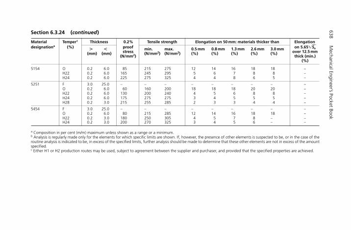
638M
echanical Engineer’s Pocket Book
Material Temperc Thickness 0.2% Tensile strength Elongation on 50 mm: materials thicker than Elongation designationa (%) � � proof min. max. 0.5 mm 0.8 mm 1.3 mm 2.6 mm 3.0 mm on 5.65���S�o
(mm) (mm) stress (N/mm2) (N/mm2) (%) (%) (%) (%) (%) over 12.5 mm(N/mm2) thick (min.)
(%)
5154 O 0.2 6.0 85 215 275 12 14 16 18 18 –H22 0.2 6.0 165 245 295 5 6 7 8 8 –H24 0.2 6.0 225 275 325 4 4 8 6 5 –
5251 F 3.0 25.0 – – – – – – – – –O 0.2 6.0 60 160 200 18 18 18 20 20 –H22 0.2 6.0 130 200 240 4 5 6 8 8 –H24 0.2 6.0 175 275 275 3 4 5 5 5 –H28 0.2 3.0 215 255 285 2 3 3 4 4 –
5454 F 3.0 25.0 – – – – – – – – –O 0.2 6.0 80 215 285 12 14 16 18 18 –H22 0.2 3.0 180 250 305 4 5 7 8 – –H24 0.2 3.0 200 270 325 3 4 5 6 – –
a Composition in per cent (m/m) maximum unless shown as a range or a minimum.b Analysis is regularly made only for the elements for which specific limits are shown. If, however, the presence of other elements is suspected to be, or in the case of theroutine analysis is indicated to be, in excess of the specified limits, further analysis should be made to determine that these other elements are not in excess of the amountspecified.c Either H1 or H2 production routes may be used, subject to agreement between the supplier and purchaser, and provided that the specified properties are achieved.
Section 6.3.24 (continued)

Engineering Materials
639
6.3.25 Aluminium alloy plate, sheet and strip: heat-treatable
Composition
Material Silicon Iron Copper Manganese Magnesium Chromium Nickel Zinc Other Titanium Aluminium Othersb
designationa (%) (%) (%) (%) (%) (%) (%) (%) restrictions (%) (%)Each Total(%)(%) (%)
2014A 0.5/0.9 0.50 3.9/5.0 0.4/1.2 0.2/0.8 0.10 0.10 0.25 0.20 Zr � Ti 0.15 Rem. 0.05 0.15
Clad 2014Ac 0.5/0.9 0.50 3.0/5.0 0.4/1.2 0.2/0.8 0.10 0.10 0.25 0.20 Zr � Ti 0.15 Rem. 0.05 0.15
2024 0.50 0.50 3.8/4.4 0.3/0.9 1.2/1.8 0.10 – 0.25 – 0.15 Rem. 0.05 0.15
Clad 2024c 0.50 0.50 3.8/4.4 0.3/0.9 1.2/1.8 0.10 – 0.25 – 0.15 Rem. 0.05 0.15
6082 0.7/1.3 0.50 0.10 0.4/1.0 0.6/1.2 0.25 – 0.20 – 0.10 Rem. 0.05 0.15
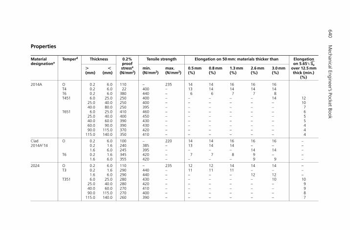
640M
echanical Engineer’s Pocket Book
Properties
Material Temperd Thickness 0.2% Tensile strength Elongation on 50 mm: materials thicker than Elongationdesignationa proof on 5.65���S�o
� � stresse over 12.5 mm(mm) (mm) (N/mm2)
min. max. 0.5 mm 0.8 mm 1.3 mm 2.6 mm 3.0 mmthick (min.) (N/mm2) (N/mm2) (%) (%) (%) (%) (%)
(%)
2014A O 0.2 6.0 110 – 235 14 14 16 16 16T4 0.2 6.0 22 400 – 13 14 14 14 14T6 0.2 6.0 380 440 – 6 6 7 7 8T451 6.0 25.0 250 400 – – – – – 14 12
25.0 40.0 250 400 – – – – – – 1040.0 80.0 250 395 – – – – – – 7
T651 6.0 25.0 410 460 – – – – – – 625.0 40.0 400 450 – – – – – – 540.0 60.0 390 430 – – – – – – 560.0 90.0 390 430 – – – – – – 490.0 115.0 370 420 – – – – – – 4
115.0 140.0 350 410 – – – – – – 4
Clad O 0.2 6.0 100 – 220 14 14 16 16 16 –2014AcT4 0.2 1.6 240 385 – 13 14 14 – – –
1.6 6.0 245 395 – – – – 14 14 –T6 0.2 1.6 345 420 – 7 7 8 9 – –
1.6 6.0 355 420 – – – – 9 9 –
2024 O 0.2 6.0 110 – 235 12 12 14 14 14 –T3 0.2 1.6 290 440 – 11 11 11 – – –
1.6 6.0 290 440 – – – – 12 12 –T351 6.0 25.0 280 430 – – – – – 10 10
25.0 40.0 280 420 – – – – – – 940.0 60.0 270 410 – – – – – – 990.0 115.0 270 400 – – – – – – 8
115.0 140.0 260 390 – – – – – – 7
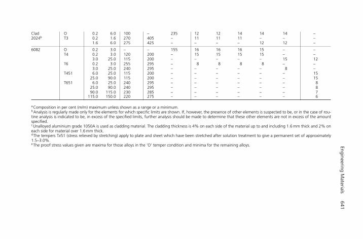
Engineering Materials
641
Clad O 0.2 6.0 100 – 235 12 12 14 14 14 –2024b T3 0.2 1.6 270 405 – 11 11 11 – – –
1.6 6.0 275 425 – – – – 12 12 –
6082 O 0.2 3.0 – – 155 16 16 16 15 – –T4 0.2 3.0 120 200 – 15 15 15 15 – –
3.0 25.0 115 200 – – – – – 15 12T6 0.2 3.0 255 295 – 8 8 8 8 – –
3.0 25.0 240 295 – – – – – 8 –T451 6.0 25.0 115 200 – – – – – – 15
25.0 90.0 115 200 – – – – – – 15T651 6.0 25.0 240 295 – – – – – – 8
25.0 90.0 240 295 – – – – – – 890.0 115.0 230 285 – – – – – – 7
115.0 150.0 220 275 – – – – – – 6
aComposition in per cent (m/m) maximum unless shown as a range or a minimum.bAnalysis is regularly made only for the elements for which specific limits are shown. If, however, the presence of other elements is suspected to be, or in the case of rou-tine analysis is indicated to be, in excess of the specified limits, further analysis should be made to determine that these other elements are not in excess of the amountspecified.cUnalloyed aluminium grade 1050A is used as cladding material. The cladding thickness is 4% on each side of the material up to and including 1.6 mm thick and 2% oneach side for material over 1.6 mm thick.dThe tempers Tx51 (stress relieved by stretching) apply to plate and sheet which have been stretched after solution treatment to give a permanent set of approximately1.5–3.0%.eThe proof stress values given are maxima for those alloys in the ‘O’ temper condition and minima for the remaining alloys.
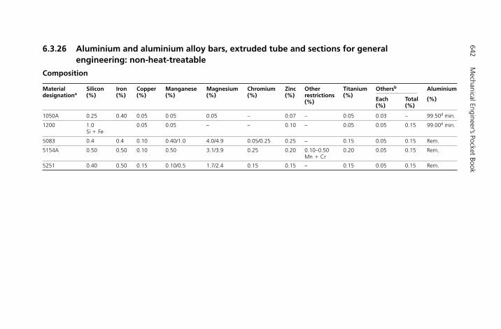
642M
echanical Engineer’s Pocket Book
6.3.26 Aluminium and aluminium alloy bars, extruded tube and sections for general engineering: non-heat-treatable
Composition
Material Silicon Iron Copper Manganese Magnesium Chromium Zinc Other Titanium Othersb Aluminiumdesignationa (%) (%) (%) (%) (%) (%) (%) restrictions (%)
Each Total (%)(%)(%) (%)
1050A 0.25 0.40 0.05 0.05 0.05 – 0.07 – 0.05 0.03 – 99.50d min.
1200 1.0 0.05 0.05 – – 0.10 – 0.05 0.05 0.15 99.00d min.Si � Fe
5083 0.4 0.4 0.10 0.40/1.0 4.0/4.9 0.05/0.25 0.25 – 0.15 0.05 0.15 Rem.
5154A 0.50 0.50 0.10 0.50 3.1/3.9 0.25 0.20 0.10–0.50 0.20 0.05 0.15 Rem.Mn � Cr
5251 0.40 0.50 0.15 0.10/0.5 1.7/2.4 0.15 0.15 – 0.15 0.05 0.15 Rem.

Engineering Materials
643
Properties
Material Temperc Diameter 0.2% Tensile strength Elongationdesignation (bar) or proof on on
thickness stress 5.65��So 50 mm(tube/sections)� � min. min. max. min. min.(mm) (mm) (N/mm2) (N/mm2) (N/mm2) (%) (%)
1050A F – – – (60) – (25) (23)
1200 F – – – (65) – (20) (18)
5083 O – 150e 125 275 – 14 13F – 150 (130) (280) – (12) (11)
5154A O – 150e 85 215 275 18 16F – 150 (100) (215) – (16) (14)
5251 F – 150 (60) (170) – (16) (14)
a Composition in per cent (m/m) maximum unless shown as a range or a minimum.b Analysis is regularly carried out for the elements for which specific limits are shown. If, however, the presence of other elem-ents is suspected to be, or in the course of routine analysis is indicated to be, in excess of specified limits, further analysisshould be made to determine that these other elements are not in excess of the amount specified.c No mechanical properties are specified for materials in the F condition. The bracketed values shown for proof stress, tensilestrength and elongation are typical properties, and are given for information only.d The aluminium content for unalloyed aluminium not made by a refining process is the difference between 100% and thesum of all other metallic elements present in amounts of 0.10% or more each, expressed to the second decimal before deter-mining the sum.e No mechanical properties are specified for tube and hollow sections having a wall thickness greater than 75 mm (see BS1474: 1987, Clause 6).
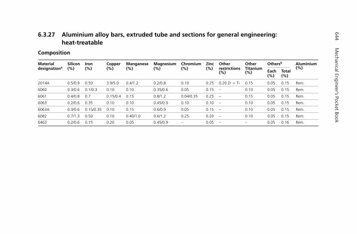
644M
echanical Engineer’s Pocket Book
6.3.27 Aluminium alloy bars, extruded tube and sections for general engineering: heat-treatable
Composition
Material Silicon Iron Copper Manganese Magnesium Chromium Zinc Other Other Othersb Aluminiumdesignationa (%) (%) (%) (%) (%) (%) (%) restrictions Titanium
Each Total(%)
(%) (%)(%) (%)
2014A 0.5/0.9 0.50 3.9/5.0 0.4/1.2 0.2/0.8 0.10 0.25 0.20 Zr � Ti 0.15 0.05 0.15 Rem.
6060 0.3/0.6 0.1/0.3 0.10 0.10 0.35/0.6 0.05 0.15 – 0.10 0.05 0.15 Rem.
6061 0.4/0.8 0.7 0.15/0.4 0.15 0.8/1.2 0.04/0.35 0.25 – 0.15 0.05 0.15 Rem.
6063 0.2/0.6 0.35 0.10 0.10 0.45/0.9 0.10 0.10 – 0.10 0.05 0.15 Rem.
6063A 0.3/0.6 0.15/0.35 0.10 0.15 0.6/0.9 0.05 0.15 – 0.10 0.05 0.15 Rem.
6082 0.7/1.3 0.50 0.10 0.40/1.0 0.6/1.2 0.25 0.20 – 0.10 0.05 0.15 Rem.
6463 0.2/0.6 0.15 0.20 0.05 0.45/0.9 – 0.05 – – 0.05 0.16 Rem.

Engineering Materials
645
Properties
Material Temperc Diameter 0.2% Tensile strength Elongationdesignationa (bar) or proof
thickness stress on on (tube/sections)d 5.65��So 50 mm
� � min. min. max. min. min.
(mm) (mm) (N/mm2) (N/mm2) (N/mm2) (%) (%)
2014A T4 – 20 230 370 – 11 1020 75 250 390 – 11 –75 150 250 390 – 8 –
T6 150 200 230 370 – 8 –– 20 370 435 – 7 6
20 75 435 480 – 7 –T6510 75 150 420 465 – 7 –
150 200 390 435 – 7 –
6060 T4 – 150 60 120 – 15 –
T5 – 150 100 145 – 8 –
T6 – 150 150 190 – 8 –
6061 T4 – 150 115 190 – 16 14
T6T6510
– 150 240 280 – 8 7
6063 O – 200 – – 140 15 13
F – 200 – (100) – (13) (12)
T4– 150 70 130 – 16 14150 200 70 120 – 13 –
T5 – 25 110 150 – 8 7
T6– 150 160 195 – 8 750 200 130 150 – 6 –
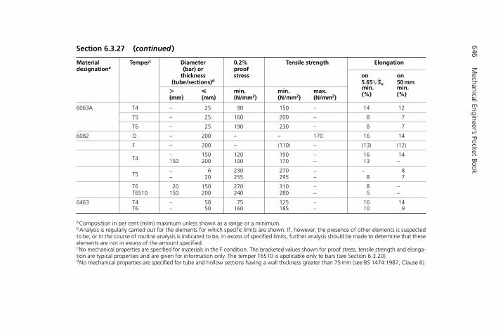
646M
echanical Engineer’s Pocket Book
Material Temperc Diameter 0.2% Tensile strength Elongationdesignationa (bar) or proof
thickness stress on on (tube/sections)d 5.65��So 50 mm
� � min. min. max. min. min.
(mm) (mm) (N/mm2) (N/mm2) (N/mm2) (%) (%)
6063A T4 – 25 90 150 – 14 12
T5 – 25 160 200 – 8 7
T6 – 25 190 230 – 8 7
6082 O – 200 – – 170 16 14
F – 200 – (110) – (13) (12)
T4– 150 120 190 – 16 14150 200 100 170 – 13 –
T5– 6 230 270 – – 8– 20 255 295 – 8 7
T6 20 150 270 310 – 8 –T6510 150 200 240 280 – 5 –
6463 T4 – 50 75 125 – 16 14T6 – 50 160 185 – 10 9
aComposition in per cent (m/m) maximum unless shown as a range or a minimum.bAnalysis is regularly carried out for the elements for which specific limits are shown. If, however, the presence of other elements is suspectedto be, or in the course of routine analysis is indicated to be, in excess of specified limits, further analysis should be made to determine that theseelements are not in excess of the amount specified.cNo mechanical properties are specified for materials in the F condition. The bracketed values shown for proof stress, tensile strength and elonga-tion are typical properties and are given for information only. The temper T6510 is applicable only to bars (see Section 6.3.20).dNo mechanical properties are specified for tube and hollow sections having a wall thickness greater than 75 mm (see BS 1474:1987, Clause 6).
Section 6.3.27 (continued )

Engineering Materials
647
6.3.28 Aluminium alloy castings, group A: general purpose
Designation LM2 LM4 LM6 LM20 LM24 LM25 LM27
Nominal Al–Si 10 Cu 2 Al–Si 5 Cu 3 Al–Si 12 Al–Si 12 Al–Si 8 Cu 3.5 Al–Si 7 Mg 0.5 Al–Si 7 Cu 2 composition Mn 0.5 Mn 0.5
Nearest alloy(s) – Al–Si 5 Cu 3 Al–Si 12 Al–Si 12 Cu Al–Si 8 Cu 3 Fe Al–Si 7 Mg Al–Si 5 Cu 3in ISO 3522 Al–Si 12 Fe Al–Si 12 Cu Fe
Elements min. max. min. max. min. max. min. max. min. max. min. max. min. max.(%) (%) (%) (%) (%) (%) (%) (%) (%) (%) (%) (%) (%) (%)
Aluminium Remainder Remainder Remainder Remainder Remainder Remainder RemainderCopper 0.7 2.5 2.0 4.0 – 0.1 – 0.4 3.0 4.0 – 0.20 1.5 2.5Magnesium – 0.3 – 0.2 – 0.1 – 0.2 – 0.30 0.2 0.6 – 0.35Silicon 9.0 11.5 4.0 6.0 10.0 13.0 10.0 13.0 7.5 9.5 6.5 7.5 6.0 8.0Iron – 1.0 – 0.8 – 0.6 – 1.0 – 1.3 – 0.5 – 0.8Manganese – 0.5 0.2 0.6 – 0.5 – 0.5 – 0.5 – 0.3 0.2 0.6Nickel – 0.5 – 0.3 – 0.1 – 0.1 – 0.5 – 0.1 – 0.3Zinc – 2.0 – 0.5 – 0.1 – 0.2 – 3.0 – 0.1 – 1.0Lead – 0.3 – 0.1 – 0.1 – 0.1 – 0.3 – 0.1 – 0.2Tin – 0.2 – 0.1 – 0.05 – 0.1 – 0.2 – 0.05 – 0.1Titanium – 0.2 – 0.2 – 0.2 – 0.2 – 0.2 – 0.2a – 0.2
Each other elementb – – – 0.05 – 0.05 – 0.05 – – – 0.05 – 0.05Total other elements – 0.5 – 0.15 – 0.15 – 0.20 – 0.5 – 0.15 – 0.15
Specified impurities are in light type. Analysis is required to verify that the contents of the specified impurities are less than the limits given in the table.Analysis for other elements is made when their presence is suspected to be in excess of the ‘each other element’ limit.a If titanium alone is used for grain refining, the amount present shall not be less than 0.05%.b In cases where alloys are required in the modified condition, the level of modifying element(s) present is not limited by the specified maximum value for other elements.
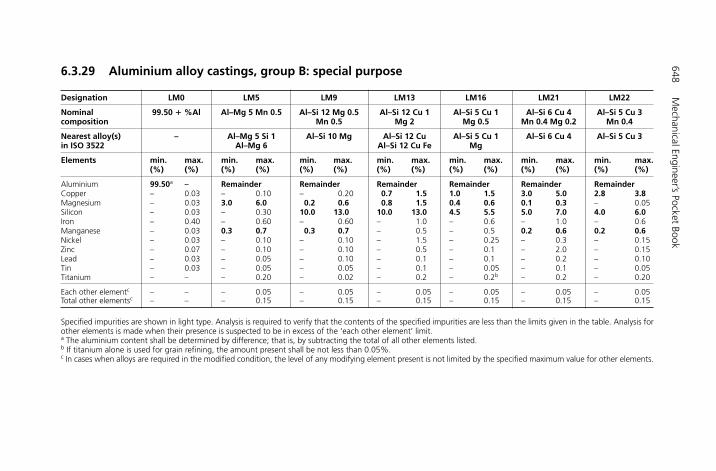
648M
echanical Engineer’s Pocket Book
6.3.29 Aluminium alloy castings, group B: special purpose
Designation LM0 LM5 LM9 LM13 LM16 LM21 LM22
Nominal 99.50 � %Al Al–Mg 5 Mn 0.5 Al–Si 12 Mg 0.5 Al–Si 12 Cu 1 Al–Si 5 Cu 1 Al–Si 6 Cu 4 Al–Si 5 Cu 3 composition Mn 0.5 Mg 2 Mg 0.5 Mn 0.4 Mg 0.2 Mn 0.4
Nearest alloy(s) – Al–Mg 5 Si 1 Al–Si 10 Mg Al–Si 12 Cu Al–Si 5 Cu 1 Al–Si 6 Cu 4 Al–Si 5 Cu 3in ISO 3522 Al–Mg 6 Al–Si 12 Cu Fe Mg
Elements min. max. min. max. min. max. min. max. min. max. min. max. min. max.(%) (%) (%) (%) (%) (%) (%) (%) (%) (%) (%) (%) (%) (%)
Aluminium 99.50a – Remainder Remainder Remainder Remainder Remainder RemainderCopper – 0.03 – 0.10 – 0.20 0.7 1.5 1.0 1.5 3.0 5.0 2.8 3.8Magnesium – 0.03 3.0 6.0 0.2 0.6 0.8 1.5 0.4 0.6 0.1 0.3 – 0.05Silicon – 0.03 – 0.30 10.0 13.0 10.0 13.0 4.5 5.5 5.0 7.0 4.0 6.0Iron – 0.40 – 0.60 – 0.60 – 1.0 – 0.6 – 1.0 – 0.6Manganese – 0.03 0.3 0.7 0.3 0.7 – 0.5 – 0.5 0.2 0.6 0.2 0.6Nickel – 0.03 – 0.10 – 0.10 – 1.5 – 0.25 – 0.3 – 0.15Zinc – 0.07 – 0.10 – 0.10 – 0.5 – 0.1 – 2.0 – 0.15Lead – 0.03 – 0.05 – 0.10 – 0.1 – 0.1 – 0.2 – 0.10Tin – 0.03 – 0.05 – 0.05 – 0.1 – 0.05 – 0.1 – 0.05Titanium – – – 0.20 – 0.02 – 0.2 – 0.2b – 0.2 – 0.20
Each other elementc – – – 0.05 – 0.05 – 0.05 – 0.05 – 0.05 – 0.05Total other elementsc – – – 0.15 – 0.15 – 0.15 – 0.15 – 0.15 – 0.15
Specified impurities are shown in light type. Analysis is required to verify that the contents of the specified impurities are less than the limits given in the table. Analysis forother elements is made when their presence is suspected to be in excess of the ‘each other element’ limit.a The aluminium content shall be determined by difference; that is, by subtracting the total of all other elements listed.b If titanium alone is used for grain refining, the amount present shall be not less than 0.05%.c In cases when alloys are required in the modified condition, the level of any modifying element present is not limited by the specified maximum value for other elements.
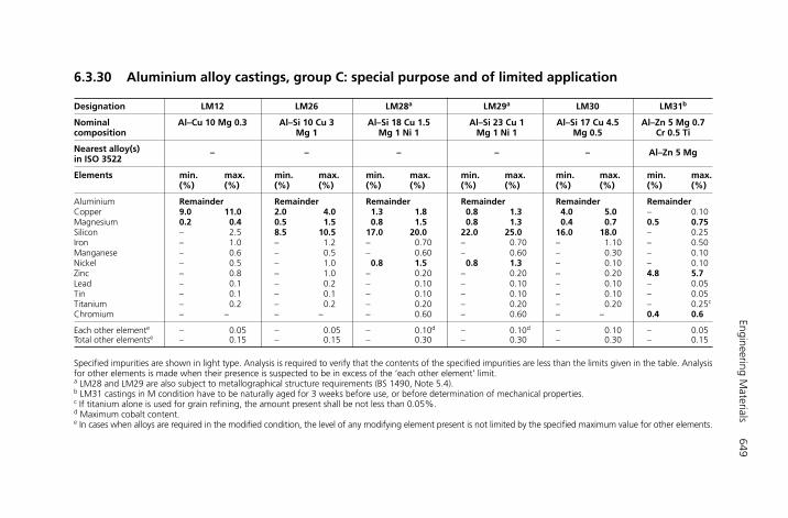
Engineering Materials
649
6.3.30 Aluminium alloy castings, group C: special purpose and of limited application
Designation LM12 LM26 LM28a LM29a LM30 LM31b
Nominal Al–Cu 10 Mg 0.3 Al–Si 10 Cu 3 Al–Si 18 Cu 1.5 Al–Si 23 Cu 1 Al–Si 17 Cu 4.5 Al–Zn 5 Mg 0.7 composition Mg 1 Mg 1 Ni 1 Mg 1 Ni 1 Mg 0.5 Cr 0.5 Ti
Nearest alloy(s) – – – – – Al–Zn 5 Mgin ISO 3522
Elements min. max. min. max. min. max. min. max. min. max. min. max.(%) (%) (%) (%) (%) (%) (%) (%) (%) (%) (%) (%)
Aluminium Remainder Remainder Remainder Remainder Remainder RemainderCopper 9.0 11.0 2.0 4.0 1.3 1.8 0.8 1.3 4.0 5.0 – 0.10Magnesium 0.2 0.4 0.5 1.5 0.8 1.5 0.8 1.3 0.4 0.7 0.5 0.75Silicon – 2.5 8.5 10.5 17.0 20.0 22.0 25.0 16.0 18.0 – 0.25Iron – 1.0 – 1.2 – 0.70 – 0.70 – 1.10 – 0.50Manganese – 0.6 – 0.5 – 0.60 – 0.60 – 0.30 – 0.10Nickel – 0.5 – 1.0 0.8 1.5 0.8 1.3 – 0.10 – 0.10Zinc – 0.8 – 1.0 – 0.20 – 0.20 – 0.20 4.8 5.7Lead – 0.1 – 0.2 – 0.10 – 0.10 – 0.10 – 0.05Tin – 0.1 – 0.1 – 0.10 – 0.10 – 0.10 – 0.05Titanium – 0.2 – 0.2 – 0.20 – 0.20 – 0.20 – 0.25c
Chromium – – – – – 0.60 – 0.60 – – 0.4 0.6
Each other elemente – 0.05 – 0.05 – 0.10d – 0.10d – 0.10 – 0.05Total other elementse – 0.15 – 0.15 – 0.30 – 0.30 – 0.30 – 0.15
Specified impurities are shown in light type. Analysis is required to verify that the contents of the specified impurities are less than the limits given in the table. Analysisfor other elements is made when their presence is suspected to be in excess of the ‘each other element’ limit.a LM28 and LM29 are also subject to metallographical structure requirements (BS 1490, Note 5.4).b LM31 castings in M condition have to be naturally aged for 3 weeks before use, or before determination of mechanical properties.c If titanium alone is used for grain refining, the amount present shall be not less than 0.05%.d Maximum cobalt content.e In cases when alloys are required in the modified condition, the level of any modifying element present is not limited by the specified maximum value for other elements.
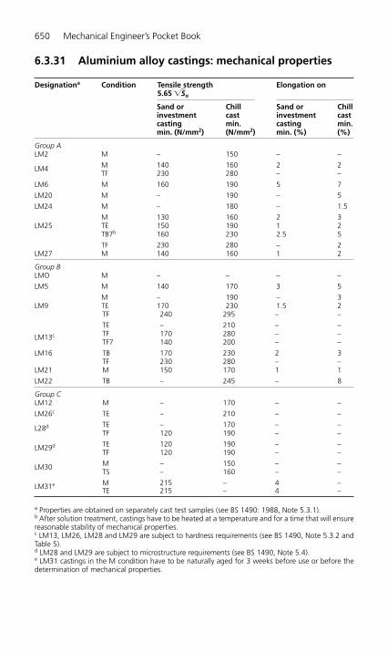
650 Mechanical Engineer’s Pocket Book
6.3.31 Aluminium alloy castings: mechanical properties
Designationa Condition Tensile strength Elongation on5.65 ��So
Sand or Chill Sand or Chill investment cast investment castcasting min. casting min.min. (N/mm2) (N/mm2) min. (%) (%)
Group ALM2 M – 150 – –
LM4 M 140 160 2 2TF 230 280 – –
LM6 M 160 190 5 7
LM20 M – 190 – 5
LM24 M – 180 – 1.5
M 130 160 2 3LM25 TE 150 190 1 2
TB7b 160 230 2.5 5
TF 230 280 – 2LM27 M 140 160 1 2
Group BLMO M – – – –
LM5 M 140 170 3 5
M – 190 – 3LM9 TE 170 230 1.5 2
TF 240 295 – –
TE – 210 – –
LM13c TF 170 280 – –TF7 140 200 – –
LM16 TB 170 230 2 3TF 230 280 – –
LM21 M 150 170 1 1
LM22 TB – 245 – 8
Group CLM12 M – 170 – –
LM26c TE – 210 – –
L28d TE – 170 – –TF 120 190 – –
LM29d TE 120 190 – –TF 120 190 – –
LM30 M – 150 – –TS – 160 – –
LM31e M 215 – 4 –TE 215 – 4 –
a Properties are obtained on separately cast test samples (see BS 1490: 1988, Note 5.3.1).b After solution treatment, castings have to be heated at a temperature and for a time that will ensurereasonable stability of mechanical properties.c LM13, LM26, LM28 and LM29 are subject to hardness requirements (see BS 1490, Note 5.3.2 andTable 5).d LM28 and LM29 are subject to microstructure requirements (see BS 1490, Note 5.4).e LM31 castings in the M condition have to be naturally aged for 3 weeks before use or before thedetermination of mechanical properties.
H6508-Ch06.3b.qxd 9/21/05 4:32 PM Page 650
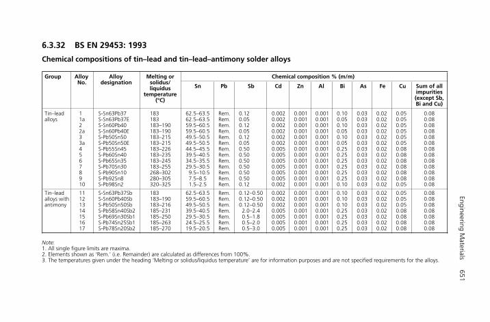
Engineering Materials
651
6.3.32 BS EN 29453: 1993
Chemical compositions of tin–lead and tin–lead–antimony solder alloys
Group Alloy Alloy Melting or Chemical composition % (m/m)No. designation solidus/
Sn Pb Sb Cd Zn Al Bi As Fe Cu Sum of all liquidus impurities temperature (except Sb, (°C)Bi and Cu)
Tin–lead 1 S-Sn63Pb37 183 62.5–63.5 Rem. 0.12 0.002 0.001 0.001 0.10 0.03 0.02 0.05 0.08alloys 1a S-Sn63Pb37E 183 62.5–63.5 Rem. 0.05 0.002 0.001 0.001 0.05 0.03 0.02 0.05 0.08
2 S-Sn60Pb40 183–190 59.5–60.5 Rem. 0.12 0.002 0.001 0.001 0.10 0.03 0.02 0.05 0.082a S-Sn60Pb40E 183–190 59.5–60.5 Rem. 0.05 0.002 0.001 0.001 0.05 0.03 0.02 0.05 0.083 S-Pb50Sn50 183–215 49.5–50.5 Rem. 0.12 0.002 0.001 0.001 0.10 0.03 0.02 0.05 0.083a S-Pb50Sn50E 183–215 49.5–50.5 Rem. 0.05 0.002 0.001 0.001 0.05 0.03 0.02 0.05 0.084 S-Pb55Sn45 183–226 44.5–45.5 Rem. 0.50 0.005 0.001 0.001 0.25 0.03 0.02 0.08 0.085 S-Pb60Sn40 183–235 39.5–40.5 Rem. 0.50 0.005 0.001 0.001 0.25 0.03 0.02 0.08 0.086 S-Pb65Sn35 183–245 34.5–35.5 Rem. 0.50 0.005 0.001 0.001 0.25 0.03 0.02 0.08 0.087 S-Pb70Sn30 183–255 29.5–30.5 Rem. 0.50 0.005 0.001 0.001 0.25 0.03 0.02 0.08 0.088 S-Pb90Sn10 268–302 9.5–10.5 Rem. 0.50 0.005 0.001 0.001 0.25 0.03 0.02 0.08 0.089 S-Pb92Sn8 280–305 7.5–8.5 Rem. 0.50 0.005 0.001 0.001 0.25 0.03 0.02 0.08 0.0810 S-Pb98Sn2 320–325 1.5–2.5 Rem. 0.12 0.002 0.001 0.001 0.10 0.03 0.02 0.05 0.08
Tin–lead 11 S-Sn63Pb37Sb 183 62.5–63.5 Rem. 0.12–0.50 0.002 0.001 0.001 0.10 0.03 0.02 0.05 0.08alloys with 12 S-Sn60Pb40Sb 183–190 59.5–60.5 Rem. 0.12–0.50 0.002 0.001 0.001 0.10 0.03 0.02 0.05 0.08antimony 13 S-Pb50Sn50Sb 183–216 49.5–50.5 Rem. 0.12–0.50 0.002 0.001 0.001 0.10 0.03 0.02 0.05 0.08
14 S-Pb58Sn40Sb2 185–231 39.5–40.5 Rem. 2.0–2.4 0.005 0.001 0.001 0.25 0.03 0.02 0.08 0.0815 S-Pb69Sn30Sb1 185–250 29.5–30.5 Rem. 0.5–1.8 0.005 0.001 0.001 0.25 0.03 0.02 0.08 0.0816 S-Pb74Sn25Sb1 185–263 24.5–25.5 Rem. 0.5–2.0 0.005 0.001 0.001 0.25 0.03 0.02 0.08 0.0817 S-Pb78Sn20Sb2 185–270 19.5–20.5 Rem. 0.5–3.0 0.005 0.001 0.001 0.25 0.03 0.02 0.08 0.08
Note:1. All single figure limits are maxima.2. Elements shown as ‘Rem.’ (i.e. Remainder) are calculated as differences from 100%.3. The temperatures given under the heading ‘Melting or solidus/liquidus temperature’ are for information purposes and are not specified requirements for the alloys.
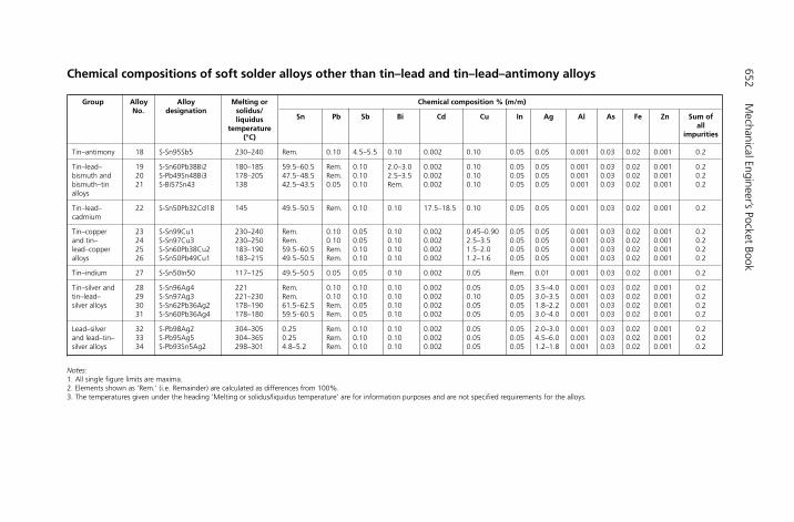
652M
echanical Engineer’s Pocket Book
Group Alloy Alloy Melting or Chemical composition % (m/m)No. designation solidus/
Sn Pb Sb Bi Cd Cu In Ag Al As Fe Zn Sum of liquidusall temperature
impurities(°C)
Tin–antimony 18 S-Sn95Sb5 230–240 Rem. 0.10 4.5–5.5 0.10 0.002 0.10 0.05 0.05 0.001 0.03 0.02 0.001 0.2
Tin–lead– 19 S-Sn60Pb38Bi2 180–185 59.5–60.5 Rem. 0.10 2.0–3.0 0.002 0.10 0.05 0.05 0.001 0.03 0.02 0.001 0.2bismuth and 20 S-Pb49Sn48Bi3 178–205 47.5–48.5 Rem. 0.10 2.5–3.5 0.002 0.10 0.05 0.05 0.001 0.03 0.02 0.001 0.2bismuth–tin 21 S-Bi57Sn43 138 42.5–43.5 0.05 0.10 Rem. 0.002 0.10 0.05 0.05 0.001 0.03 0.02 0.001 0.2alloys
Tin–lead– 22 S-Sn50Pb32Cd18 145 49.5–50.5 Rem. 0.10 0.10 17.5–18.5 0.10 0.05 0.05 0.001 0.03 0.02 0.001 0.2cadmium
Tin–copper 23 S-Sn99Cu1 230–240 Rem. 0.10 0.05 0.10 0.002 0.45–0.90 0.05 0.05 0.001 0.03 0.02 0.001 0.2and tin– 24 S-Sn97Cu3 230–250 Rem. 0.10 0.05 0.10 0.002 2.5–3.5 0.05 0.05 0.001 0.03 0.02 0.001 0.2lead–copper 25 S-Sn60Pb38Cu2 183–190 59.5–60.5 Rem. 0.10 0.10 0.002 1.5–2.0 0.05 0.05 0.001 0.03 0.02 0.001 0.2alloys 26 S-Sn50Pb49Cu1 183–215 49.5–50.5 Rem. 0.10 0.10 0.002 1.2–1.6 0.05 0.05 0.001 0.03 0.02 0.001 0.2
Tin–indium 27 S-Sn50In50 117–125 49.5–50.5 0.05 0.05 0.10 0.002 0.05 Rem. 0.01 0.001 0.03 0.02 0.001 0.2
Tin–silver and 28 S-Sn96Ag4 221 Rem. 0.10 0.10 0.10 0.002 0.05 0.05 3.5–4.0 0.001 0.03 0.02 0.001 0.2tin–lead– 29 S-Sn97Ag3 221–230 Rem. 0.10 0.10 0.10 0.002 0.10 0.05 3.0–3.5 0.001 0.03 0.02 0.001 0.2silver alloys 30 S-Sn62Pb36Ag2 178–190 61.5–62.5 Rem. 0.05 0.10 0.002 0.05 0.05 1.8–2.2 0.001 0.03 0.02 0.001 0.2
31 S-Sn60Pb36Ag4 178–180 59.5–60.5 Rem. 0.05 0.10 0.002 0.05 0.05 3.0–4.0 0.001 0.03 0.02 0.001 0.2
Lead–silver 32 S-Pb98Ag2 304–305 0.25 Rem. 0.10 0.10 0.002 0.05 0.05 2.0–3.0 0.001 0.03 0.02 0.001 0.2and lead–tin– 33 S-Pb95Ag5 304–365 0.25 Rem. 0.10 0.10 0.002 0.05 0.05 4.5–6.0 0.001 0.03 0.02 0.001 0.2silver alloys 34 S-Pb93Sn5Ag2 298–301 4.8–5.2 Rem. 0.10 0.10 0.002 0.05 0.05 1.2–1.8 0.001 0.03 0.02 0.001 0.2
Chemical compositions of soft solder alloys other than tin–lead and tin–lead–antimony alloys
Notes:1. All single figure limits are maxima.2. Elements shown as ‘Rem.’ (i.e. Remainder) are calculated as differences from 100%.3. The temperatures given under the heading ‘Melting or solidus/liquidus temperature’ are for information purposes and are not specified requirements for the alloys.
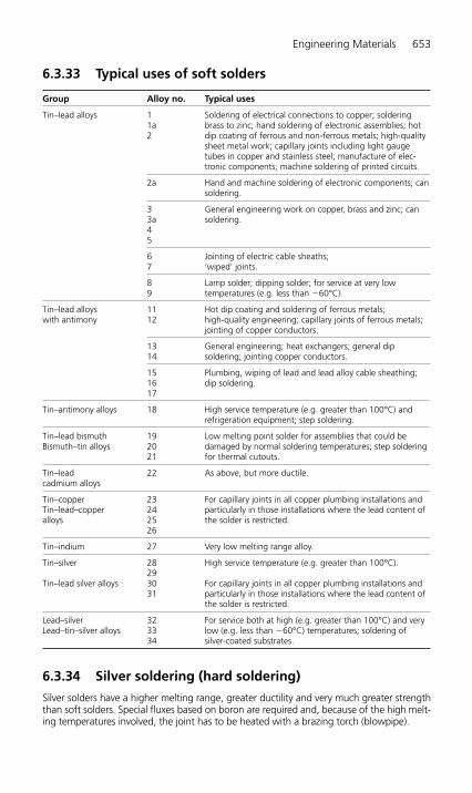
6.3.33 Typical uses of soft solders
Group Alloy no. Typical uses
Tin–lead alloys 1 Soldering of electrical connections to copper; soldering 1a brass to zinc; hand soldering of electronic assemblies; hot 2 dip coating of ferrous and non-ferrous metals; high-quality
sheet metal work; capillary joints including light gaugetubes in copper and stainless steel; manufacture of elec-tronic components; machine soldering of printed circuits.
2a Hand and machine soldering of electronic components; cansoldering.
3 General engineering work on copper, brass and zinc; can 3a soldering.45
6 Jointing of electric cable sheaths;7 ‘wiped’ joints.
8 Lamp solder; dipping solder; for service at very low 9 temperatures (e.g. less than �60°C).
Tin–lead alloys 11 Hot dip coating and soldering of ferrous metals; with antimony 12 high-quality engineering; capillary joints of ferrous metals;
jointing of copper conductors.
13 General engineering; heat exchangers; general dip 14 soldering; jointing copper conductors.
15 Plumbing, wiping of lead and lead alloy cable sheathing; 16 dip soldering.17
Tin–antimony alloys 18 High service temperature (e.g. greater than 100°C) andrefrigeration equipment; step soldering.
Tin–lead bismuth 19 Low melting point solder for assemblies that could be Bismuth–tin alloys 20 damaged by normal soldering temperatures; step soldering
21 for thermal cutouts.
Tin–lead 22 As above, but more ductile.cadmium alloys
Tin–copper 23 For capillary joints in all copper plumbing installations andTin–lead–copper 24 particularly in those installations where the lead content of alloys 25 the solder is restricted.
26
Tin–indium 27 Very low melting range alloy.
Tin–silver 28 High service temperature (e.g. greater than 100°C).29
Tin–lead silver alloys 30 For capillary joints in all copper plumbing installations and 31 particularly in those installations where the lead content of
the solder is restricted.
Lead–silver 32 For service both at high (e.g. greater than 100°C) and very Lead–tin–silver alloys 33 low (e.g. less than �60°C) temperatures; soldering of
34 silver-coated substrates.
6.3.34 Silver soldering (hard soldering)
Silver solders have a higher melting range, greater ductility and very much greater strengththan soft solders. Special fluxes based on boron are required and, because of the high melt-ing temperatures involved, the joint has to be heated with a brazing torch (blowpipe).
Engineering Materials 653
H6508-Ch06.3b.qxd 9/21/05 4:32 PM Page 653

654M
echanical Engineer’s Pocket Book
Type Composition (% by mass) Melting range (approximately)
Silver Copper Zinc Cadmiuma Tin Manganese Nickel Impurity limits applicable Solidus Liquidusto all types
min. max. min. max. min. max. min. max. min. max. min. max. min. max. max. (°C) (°C)
AG1 49.0 51.0 14.0 16.0 14.0 18.0 18.0 20.0 – – – – – – Aluminium 0.0010 620 640AG2 41.0 43.0 16.0 18.0 14.0 18.0 24.0 26.0 – – – – – – Beryllium 0.0005 610 620AG3 37.0 39.0 19.0 21.0 20.0 24.0 19.0 21.0 – – – – – – Bismuth 0.005 605 650AG11 33.0 35.0 24.0 26.0 18.0 22.0 20.0 22.0 – – – – – – Lead 0.025 610 670AG12 29.0 31.0 27.0 29.0 19.0 23.0 20.0 22.0 – – – – – – Phosphorus 0.008 600 690
Silicon 0.05AG14 54.0 56.0 20.0 22.0 21.0 23.0 – 0.025 1.7 2.3 – – – – Titanium 0.002 630 660AG20b 39.0 41.0 29.0 31.0 27.0 29.0 – 0.025 1.7 2.3 – – – – Zirconium 0.002 650 710AG21b 29.0 31.0 35.0 37.0 31.0 33.0 – 0.025 1.7 2.3 – – – – 665 755
Total of all impurities 0.25AG5 42.0 44.0 36.0 38.0 18.0 22.0 – 0.025 – – – – – – 690 770AG7c 71.0 73.0 27.0 29.0 – – – 0.025 – – – – – – 780 780AG9 49.0 51.0 14.5 16.5 13.5 17.5 15.0 17.0 – – – – 2.5 3.5 635 655AG13 59.0 61.0 25.0 27.0 12.0 16.0 – 0.025 – – – – – – 695 730AG18 48.0 50.0 15.0 17.0 21.0 25.0 – 0.025 – – 6.5 8.5 4.0 5.0 680 705AG19 84.0 86.0 – – – – – 0.025 – – 14.0 16.0 – – 960 970
6.3.35 Group AG: silver brazing filler metals
aFiller metals containing cadmium produce fumes during brazing that, if inhaled, can be dangerous to health. In view of the low-threshold limit value (TLV) for cadmium oxide, 0.05 mg/m2, it is recommendedthat a local extraction system is used during brazing.bAttention is drawn to the fact that it is claimed that AG20 and AG21 are the subject of British patent No. 1436943 and No. 1532879, respectively, copies of which can be obtained from the Patent Office, 25 Southampton Buildings, London WC2A 1AY. BSI takes no position as to the validity of the patents or whether they are still in force. The patents are irrevocably endorsed ‘licences of right’ under Section 46of the Patents Act 1977 (or Section 35(2)(a) of the Patents Act 1949 if applicable), which states:
‘(3) Where such an entry is made in respect of a patent:
(a) any person shall, at any time after the entry is made, be entitled as of right to a licence under the patent on such terms as may be settled by agreement or, in default of agreement, by the Comptrolleron the application of the proprietor of the patent or the person requiring the licence.’
Licence details may be obtained from the registered proprietors of the patents.cSuitable for vacuum applications. For the full range of filler metals (spelters) for brazing, see BS 1845.

Engineering Materials 655
6.4 Metallic material sizes
6.4.1 Metallic material sizes: introduction to BS 6722: 1986
British Standard BS 6722 supersedes BS 4229 Parts 1 and 2, BS 4391 and DD5 which arenow withdrawn.
In the case of wire, the dimensions recommended are those previously given in BS 4391,since they are firmly and logically established in the wire and associated industries.
For other products where a clear pattern of sizes does not exist, and where availability anddemand vary from one sector of industry to another, it was considered that a list of rec-ommended dimensions based on the rounded R20 series (BS 2045) should be establishedwithout any attempt to distinguish between product types or between ferrous and non-ferrous materials. Suitable dimensions may then be drawn from this list to establish arange of sizes to meet best the pattern of demand.
The detailed recommendations for bar shapes previously given in BS 4229 have not there-fore been included. In a similar way, the recommendations previously given in DD5 forplate and sheet have been rationalized and the recommendations for thickness of sheetand plate are now referenced as for bar dimensions. Details of preferred sizes for hexa-gon bars are given in BS 3692.
It is recommended that applicable British Standards for metallic materials should includecombinations of dimensions recommended in BS 6722: 1986. BS 6722 gives recom-mended dimensions for use as a basis for establishing the sizes of metallic materials in theform of wires, bars (excluding hexagon bars) and flat products including sheet and plate:
Wires The diameters of wires should be selected from the recommended dimensionsgiven in Section 6.4.2.
Bars The diameters of round bars and the thickness and widths of bars of rectangularor square cross section should be selected from the recommended dimensions given inSection 6.4.3.
Flat products The widths and/or lengths for flat products (sheet, strip and plate)should be selected from the recommended dimensions given in Section 6.4.4. The thick-nesses for flat products should be selected from the recommended dimensions given inSection 6.4.3.
H6508-Ch06.4.qxd 9/12/05 4:51 PM Page 655
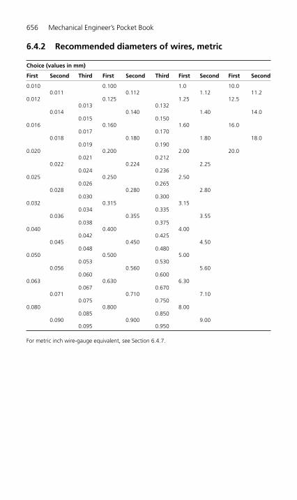
656 Mechanical Engineer’s Pocket Book
Choice (values in mm)
First Second Third First Second Third First Second First Second
0.010 0.100 1.0 10.00.011 0.112 1.12 11.2
0.012 0.125 1.25 12.50.013 0.132
0.014 0.140 1.40 14.00.015 0.150
0.016 0.160 1.60 16.00.017 0.170
0.018 0.180 1.80 18.00.019 0.190
0.020 0.200 2.00 20.00.021 0.212
0.022 0.224 2.250.024 0.236
0.025 0.250 2.500.026 0.265
0.028 0.280 2.800.030 0.300
0.032 0.315 3.150.034 0.335
0.036 0.355 3.550.038 0.375
0.040 0.400 4.000.042 0.425
0.045 0.450 4.500.048 0.480
0.050 0.500 5.000.053 0.530
0.056 0.560 5.600.060 0.600
0.063 0.630 6.300.067 0.670
0.071 0.710 7.100.075 0.750
0.080 0.800 8.000.085 0.850
0.090 0.900 9.000.095 0.950
For metric inch wire-gauge equivalent, see Section 6.4.7.
6.4.2 Recommended diameters of wires, metric
H6508-Ch06.4.qxd 9/12/05 4:51 PM Page 656

Engineering Materials 657
6.4.3 Recommended dimensions for bar and flat products
Choice (values in mm)
First Second First Second First Second First Second
0.10 1.0 10.0 1000.11 1.1 11.0 110
0.12 1.2 12.0 1200.14 1.4 14.0 140
0.16 1.6 16.0 1600.18 1.8 18.0 180
0.20 2.0 20.0 2000.22 2.2 22.0 220
0.25 2.5 25.0 2500.28 2.8 28.0 280
0.30 3.0 30.0 3000.35 3.5 35.0
0.40 4.0 40.00.45 4.5 45.0
0.50 5.0 50.00.55 5.5 55.0
0.60 6.0 60.00.70 7.0 70.0
0.80 8.0 80.00.90 9.0 90.0
6.4.4 Recommended widths and lengths of flat products
Width (mm) Length (mm)
400 2500500 3000600 4000800 5000
1000 60001200 80001250 1000015002000
H6508-Ch06.4.qxd 9/12/05 4:51 PM Page 657
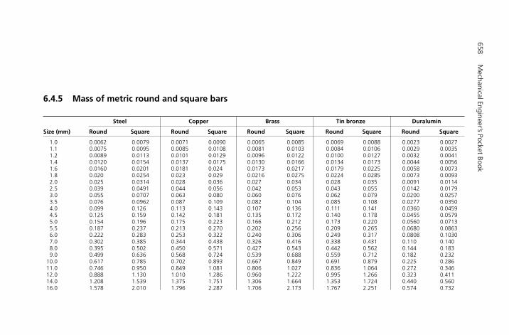
658M
echanical Engineer’s Pocket Book
6.4.5 Mass of metric round and square bars
Steel Copper Brass Tin bronze Duralumin
Size (mm) Round Square Round Square Round Square Round Square Round Square
1.0 0.0062 0.0079 0.0071 0.0090 0.0065 0.0085 0.0069 0.0088 0.0023 0.00271.1 0.0075 0.0095 0.0085 0.0108 0.0081 0.0103 0.0084 0.0106 0.0029 0.00351.2 0.0089 0.0113 0.0101 0.0129 0.0096 0.0122 0.0100 0.0127 0.0032 0.00411.4 0.0120 0.0154 0.0137 0.0175 0.0130 0.0166 0.0134 0.0173 0.0044 0.00561.6 0.0160 0.0201 0.0181 0.024 0.0173 0.0217 0.0179 0.0225 0.0058 0.00731.8 0.020 0.0254 0.023 0.029 0.0216 0.0275 0.0224 0.0285 0.0073 0.00932.0 0.025 0.0314 0.028 0.036 0.027 0.034 0.028 0.035 0.0091 0.01142.5 0.039 0.0491 0.044 0.056 0.042 0.053 0.043 0.055 0.0142 0.01793.0 0.055 0.0707 0.063 0.080 0.060 0.076 0.062 0.079 0.0200 0.02573.5 0.076 0.0962 0.087 0.109 0.082 0.104 0.085 0.108 0.0277 0.03504.0 0.099 0.126 0.113 0.143 0.107 0.136 0.111 0.141 0.0360 0.04594.5 0.125 0.159 0.142 0.181 0.135 0.172 0.140 0.178 0.0455 0.05795.0 0.154 0.196 0.175 0.223 0.166 0.212 0.173 0.220 0.0560 0.07135.5 0.187 0.237 0.213 0.270 0.202 0.256 0.209 0.265 0.0680 0.08636.0 0.222 0.283 0.253 0.322 0.240 0.306 0.249 0.317 0.0808 0.10307.0 0.302 0.385 0.344 0.438 0.326 0.416 0.338 0.431 0.110 0.1408.0 0.395 0.502 0.450 0.571 0.427 0.543 0.442 0.562 0.144 0.1839.0 0.499 0.636 0.568 0.724 0.539 0.688 0.559 0.712 0.182 0.232
10.0 0.617 0.785 0.702 0.893 0.667 0.849 0.691 0.879 0.225 0.28611.0 0.746 0.950 0.849 1.081 0.806 1.027 0.836 1.064 0.272 0.34612.0 0.888 1.130 1.010 1.286 0.960 1.222 0.995 1.266 0.323 0.41114.0 1.208 1.539 1.375 1.751 1.306 1.664 1.353 1.724 0.440 0.56016.0 1.578 2.010 1.796 2.287 1.706 2.173 1.767 2.251 0.574 0.732
Engineering Materials
659
18.0 1.998 2.543 2.274 2.894 2.160 2.749 2.238 2.848 0.727 0.92620.0 2.466 3.140 2.806 3.573 2.666 3.394 2.762 3.517 0.898 1.14325.0 3.853 4.906 4.385 5.583 4.165 5.303 4.315 5.495 1.402 1.78630.0 5.158 7.065 5.870 8.040 5.876 7.637 5.777 7.913 1.878 2.57235.0 7.553 9.616 8.595 10.943 8.165 10.395 8.459 10.770 2.749 3.50040.0 9.865 12.56 11.23 14.29 10.66 13.58 11.05 14.07 3.590 4.57245.0 12.48 15.90 14.20 18.09 13.49 17.19 13.98 17.81 4.542 5.78850.0 15.41 19.63 17.54 22.34 16.66 21.22 17.26 21.99 5.609 7.14555.0 18.65 23.75 21.22 27.03 20.16 25.67 20.89 26.60 6.789 8.64560.0 22.20 28.26 25.26 32.16 24.00 30.55 24.86 31.65 8.081 10.2970.0 30.21 38.47 34.38 43.78 32.66 41.59 33.84 43.09 11.00 14.0080.0 39.46 50.24 44.91 57.17 42.66 54.31 44.20 56.27 14.36 18.2990.0 49.94 63.59 56.83 72.37 53.99 68.74 55.93 71.22 18.18 23.15
100.0 61.65 78.50 70.16 89.33 66.64 84.86 69.05 87.92 22.44 28.57120.0 88.78 113.04 101.03 128.64 95.97 122.20 99.43 126.60 32.32 41.15160.0 167.84 200.96 191.00 228.69 181.44 217.24 187.98 225.08 61.09 73.15200.0 246.60 314.00 280.63 319.36 266.58 339.43 276.19 351.68 89.76 114.30250.0 385.31 490.63 438.48 558.34 416.52 530.37 431.55 549.51 140.25 178.59300.0 554.80 706.50 631.36 804.00 599.74 763.73 621.38 791.28 201.95 257.17
Values in kg/m.

660 Mechanical Engineer’s Pocket Book
6.4.6 Hexagon bar sizes for screwed fasteners, metric
Choice Nominal size Hexagon bar sizes (mm) Mass (kg/m) of thread A/F A/C (max. bar size:
max. min. max. min.steel)
M1.6 3.2 3.08 3.7 3.48 0.07M2 4.0 3.88 4.6 4.38 0.11M2.5 5.0 4.88 5.8 5.51 0.17
First M3 5.5 5.38 6.4 6.08 0.21(preferred) M4 7.0 6.85 8.1 7.74 0.33
M5 8.0 7.85 9.2 8.87 0.44M6 10.0 9.78 11.5 11.05 0.68M8 13.0 12.73 15.0 14.38 1.15M10 17.0 16.73 19.6 18.90 1.97M12 19.0 18.67 21.9 21.10 2.45M16 24.0 23.67 27.7 26.75 3.62M20 30.0 29.67 34.6 33.53 6.12M24 36.0 35.38 41.6 39.98 8.81M30 46.0 45.38 53.1 51.28 14.40M36 55.0 54.26 63.5 61.31 20.52M42 65.0 64.26 75.1 72.61 28.67M48 75.0 74.26 86.6 83.91 35.15M56 85.0 84.13 98.1 95.07 49.00M64 95.0 94.13 109.7 106.37 61.22
M14 22.0 21.67 25.4 24.49 3.29M18 27.0 26.67 31.2 30.14 4.95
Second M22 32.0 31.61 36.9 35.74 6.96(non-preferred) M27 41.0 40.38 47.3 45.63 11.43
M33 50.0 49.38 57.7 55.80 17.00M39 60.0 59.26 69.3 66.96 24.42M45 70.0 69.26 80.8 78.26 32.23M52 80.0 79.26 92.4 89.56 43.41M60 90.0 89.13 103.9 100.72 55.00M68 100.0 99.13 115.5 112.02 67.84
The mass of common non-ferrous hexagon bars can be determined by multiplying themass of a corresponding steel bar by one of the following conversion factors:
Brass � 1.081Bronze � 1.120Duralumin � 0.364.
For example, the mass of a hexagonal steel bar 30 mm across flats (A/F) is 6.12 kg/m. Thusthe mass of a hexagonal brass bar 30 mm A/F is 6.12 � 1.081 � 6.616 kg/m.
A/F: across flats; A/C: across corners.
H6508-Ch06.4.qxd 9/12/05 4:51 PM Page 660
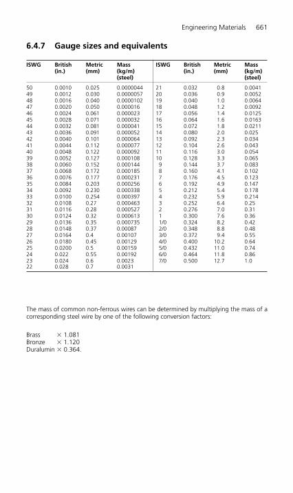
Engineering Materials 661
6.4.7 Gauge sizes and equivalents
ISWG British Metric Mass ISWG British Metric Mass (in.) (mm) (kg/m) (in.) (mm) (kg/m)
(steel) (steel)
50 0.0010 0.025 0.0000044 21 0.032 0.8 0.004149 0.0012 0.030 0.0000057 20 0.036 0.9 0.005248 0.0016 0.040 0.0000102 19 0.040 1.0 0.006447 0.0020 0.050 0.000016 18 0.048 1.2 0.009246 0.0024 0.061 0.000023 17 0.056 1.4 0.012545 0.0028 0.071 0.000032 16 0.064 1.6 0.016344 0.0032 0.081 0.000041 15 0.072 1.8 0.021143 0.0036 0.091 0.000052 14 0.080 2.0 0.02542 0.0040 0.101 0.000064 13 0.092 2.3 0.03441 0.0044 0.112 0.000077 12 0.104 2.6 0.04340 0.0048 0.122 0.000092 11 0.116 3.0 0.05439 0.0052 0.127 0.000108 10 0.128 3.3 0.06538 0.0060 0.152 0.000144 9 0.144 3.7 0.08337 0.0068 0.172 0.000185 8 0.160 4.1 0.10236 0.0076 0.177 0.000231 7 0.176 4.5 0.12335 0.0084 0.203 0.000256 6 0.192 4.9 0.14734 0.0092 0.230 0.000338 5 0.212 5.4 0.17833 0.0100 0.254 0.000397 4 0.232 5.9 0.21432 0.0108 0.27 0.000463 3 0.252 6.4 0.2531 0.0116 0.28 0.000527 2 0.276 7.0 0.3130 0.0124 0.32 0.000613 1 0.300 7.6 0.3629 0.0136 0.35 0.000735 1/0 0.324 8.2 0.4228 0.0148 0.37 0.00087 2/0 0.348 8.8 0.4827 0.0164 0.4 0.00107 3/0 0.372 9.4 0.5526 0.0180 0.45 0.00129 4/0 0.400 10.2 0.6425 0.0200 0.5 0.00159 5/0 0.432 11.0 0.7424 0.022 0.55 0.00192 6/0 0.464 11.8 0.8623 0.024 0.6 0.0023 7/0 0.500 12.7 1.022 0.028 0.7 0.0031
The mass of common non-ferrous wires can be determined by multiplying the mass of acorresponding steel wire by one of the following conversion factors:
Brass � 1.081Bronze � 1.120Duralumin � 0.364.
H6508-Ch06.4.qxd 9/12/05 4:51 PM Page 661
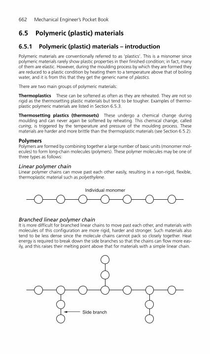
662 Mechanical Engineer’s Pocket Book
6.5 Polymeric (plastic) materials
6.5.1 Polymeric (plastic) materials – introduction
Polymeric materials are conventionally referred to as ‘plastics’. This is a misnomer sincepolymeric materials rarely show plastic properties in their finished condition; in fact, manyof them are elastic. However, during the moulding process by which they are formed theyare reduced to a plastic condition by heating them to a temperature above that of boilingwater, and it is from this that they get the generic name of plastics.
There are two main groups of polymeric materials:
Thermoplastics These can be softened as often as they are reheated. They are not sorigid as the thermosetting plastic materials but tend to be tougher. Examples of thermo-plastic polymeric materials are listed in Section 6.5.3.
Thermosetting plastics (thermosets) These undergo a chemical change duringmoulding and can never again be softened by reheating. This chemical change, calledcuring, is triggered by the temperature and pressure of the moulding process. Thesematerials are harder and more brittle than the thermoplastic materials (see Section 6.5.2).
PolymersPolymers are formed by combining together a large number of basic units (monomer mol-ecules) to form long-chain molecules (polymers). These polymer molecules may be one ofthree types as follows:
Linear polymer chainLinear polymer chains can move past each other easily, resulting in a non-rigid, flexible,thermoplastic material such as polyethylene.
Branched linear polymer chainIt is more difficult for branched linear chains to move past each other, and materials withmolecules of this configuration are more rigid, harder and stronger. Such materials alsotend to be less dense since the molecule chains cannot pack so closely together. Heatenergy is required to break down the side branches so that the chains can flow more eas-ily, and this raises their melting point above that for materials with a simple linear chain.
Individual monomer
Side branch
H6508-Ch06.5.qxd 9/12/05 4:53 PM Page 662

Engineering Materials 663
Cross-linked polymerThe cross-linked molecular chain is typical of the thermosetting plastics. Thermosets arerigid and tend to be brittle once the cross-links are formed by ‘curing’ the material duringthe moulding process. The elastomers are an intermediate group of materials whichexhibit the toughness and resilience of rubber. This is achieved by a more limited cross-linking than that of the rigid thermosets.
Reinforced polymeric materialsIn this group of materials synthetic, polymeric materials are used to bond together strongreinforcing materials to produce high-strength composites.
Glass-reinforced plastics (GRP)High-strength glass fibres are bonded together using polyester or epoxide resins. The fibresmay be in the form of rovings (ropes), woven cloth or chopped strand mat. GRP are usedfor a wide range of products, including: printed circuit boards for high-quality electronicequipment, safety helmets, and boat hulls and superstructures.
Laminated plasticsSheets of paper, cotton cloth, woollen cloth or woven glass fibre are impregnated with anappropriate synthetic resin and then stacked between polished metal sheets in a hydraulicpress. The combined heat and pressure cause the laminates to bond together and to cure.The moulded sheets, rods, tubes and other sections produced by the process have highstrength and can be machined on conventional machined tools into screwed fastenings,bushes, gears, etc. in a manner similar to metals. A typical range of such materials is avail-able under the trade name of Tufnol.
AdhesivesFor detail, see Section 4.5.
Cross-link Cross-link
H6508-Ch06.5.qxd 9/12/05 4:53 PM Page 663

664 Mechanical Engineer’s Pocket Book
6.5.2 Some important thermosetting polymers
Material Relative Tensile Elongation Impact Maximum density strength (%) strength service
(N/mm2) (J) temperature (°C)
Phenol formaldehydea 1.35 35–55 1.0 0.3–1.5 75Urea formaldehydeb 1.50 50–75 1.0 0.3–0.5 75Melamine formaldehydeb 1.50 56–80 0.7 0.2–0.4 100Casein (cross-linked 1.34 55–70 2.5–4.0 1.5–2.0 150
with formaldehyde)Epoxidesc 1.15 35–80 5.0–10.0 0.5–1.5 200Polyesters (unsaturated) 1.12 50–60 2.0 0.7 220Polyesters (alkyd resins) 2.00 20–30 0.0 0.25 150Silicones 1.88 35–45 30–40 0.4 450
a With wood flour filler.b With cellulose filler.c Rigid, unfilled.
AdditivesPlasticizers These reduce the rigidity and brittleness of polymeric materials and improvetheir flow properties during moulding.
Fillers These are bulking agents which not only reduce the cost of the moulding pow-der, but have a considerable influence on the properties of a moulding produced from agiven polymeric material. Fillers improve the impact strength and reduce shrinkage duringmoulding. Typical fillers are:
Glass fibre: good electrical properties.Wood flour, calcium carbonate: low cost, high bulk, low strength.Aluminium powder: expensive but high strength and wear resistance.Shredded paper (cellulose), shredded cloth: good mechanical strength with reason-able electrical insulation properties.Mica granules: good heat resistance and good electrical insulation properties.
Stabilizers These are added to prevent or reduce degradation, and include antioxi-dants, antiozonants and ultraviolet ray absorbants.
Colourants These can be subdivided into dyestuffs, organic pigments and inorganic pig-ments. Dyestuffs are used for transparent and translucent plastics. Pigments have greateropacity, colour stability and heat stability than dyestuffs. They are unsuitable for transparentplastics.
Antistatic agents These provide improved surface conductivity so that static electricalcharges can leak away, thus reducing the attraction of dust particles, the risk of electricshock and the risk of explosion in hazardous environments caused by the spark associatedwith an electrical discharge.
H6508-Ch06.5.qxd 9/12/05 4:53 PM Page 664
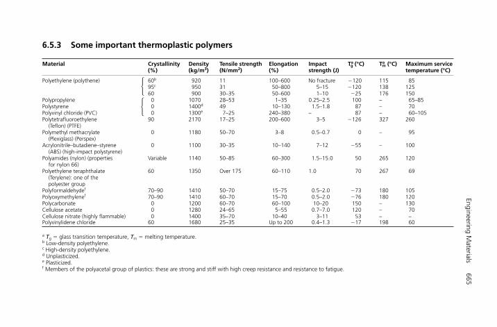
Engineering Materials
665
6.5.3 Some important thermoplastic polymers
Material Crystallinity Density Tensile strength Elongation Impact Tag (°C) Ta
m (°C) Maximum service(%) (kg/m3) (N/mm2) (%) strength (J) temperature (°C)
Polyethylene (polythene) 60b 920 11 100–600 No fracture �120 115 8595c 950 31 50–800 5–15 �120 138 12560 900 30–35 50–600 1–10 �25 176 150
Polypropylene 0 1070 28–53 1–35 0.25–2.5 100 – 65–85Polystyrene 0 1400d 49 10–130 1.5–1.8 87 – 70Polyvinyl chloride (PVC) 0 1300e 7–25 240–380 – 87 – 60–105Polytetrafluoroethylene 90 2170 17–25 200–600 3–5 �126 327 260
(Teflon) (PTFE)Polymethyl methacrylate 0 1180 50–70 3–8 0.5–0.7 0 – 95
(Plexiglass) (Perspex)Acrylonitrile–butadiene–styrene 0 1100 30–35 10–140 7–12 �55 – 100
(ABS) (high-impact polystyrene)Polyamides (nylon) (properties Variable 1140 50–85 60–300 1.5–15.0 50 265 120
for nylon 66)Polyethylene teraphthalate 60 1350 Over 175 60–110 1.0 70 267 69
(Terylene): one of the polyester group
Polyformaldehydef 70–90 1410 50–70 15–75 0.5–2.0 �73 180 105Polyoxymethylenef 70–90 1410 60–70 15–70 0.5–2.0 �76 180 120Polycarbonate 0 1200 60–70 60–100 10–20 150 – 130Cellulose acetate 0 1280 24–65 5–55 0.7–7.0 120 – 70Cellulose nitrate (highly flammable) 0 1400 35–70 10–40 3–11 53 – –Polyvinylidene chloride 60 1680 25–35 Up to 200 0.4–1.3 �17 198 60
a Tg � glass transition temperature, Tm � melting temperature.b Low-density polyethylene.c High-density polyethylene.d Unplasticized.e Plasticized.f Members of the polyacetal group of plastics: these are strong and stiff with high creep resistance and resistance to fatigue.
��
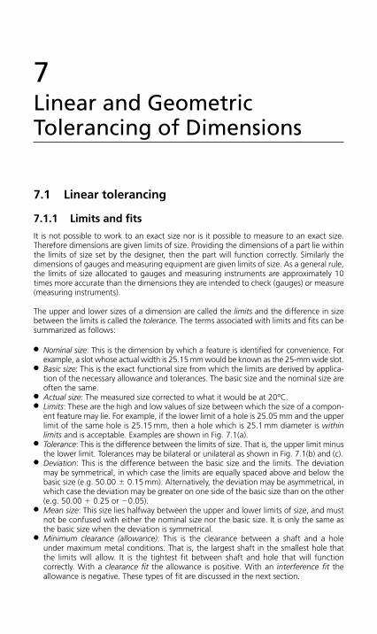
7Linear and GeometricTolerancing of Dimensions
7.1 Linear tolerancing
7.1.1 Limits and fits
It is not possible to work to an exact size nor is it possible to measure to an exact size.Therefore dimensions are given limits of size. Providing the dimensions of a part lie withinthe limits of size set by the designer, then the part will function correctly. Similarly thedimensions of gauges and measuring equipment are given limits of size. As a general rule,the limits of size allocated to gauges and measuring instruments are approximately 10times more accurate than the dimensions they are intended to check (gauges) or measure(measuring instruments).
The upper and lower sizes of a dimension are called the limits and the difference in sizebetween the limits is called the tolerance. The terms associated with limits and fits can besummarized as follows:
● Nominal size: This is the dimension by which a feature is identified for convenience. Forexample, a slot whose actual width is 25.15 mm would be known as the 25-mm wide slot.
● Basic size: This is the exact functional size from which the limits are derived by applica-tion of the necessary allowance and tolerances. The basic size and the nominal size areoften the same.
● Actual size: The measured size corrected to what it would be at 20°C.● Limits: These are the high and low values of size between which the size of a compon-
ent feature may lie. For example, if the lower limit of a hole is 25.05 mm and the upperlimit of the same hole is 25.15 mm, then a hole which is 25.1 mm diameter is withinlimits and is acceptable. Examples are shown in Fig. 7.1(a).
● Tolerance: This is the difference between the limits of size. That is, the upper limit minusthe lower limit. Tolerances may be bilateral or unilateral as shown in Fig. 7.1(b) and (c).
● Deviation: This is the difference between the basic size and the limits. The deviationmay be symmetrical, in which case the limits are equally spaced above and below thebasic size (e.g. 50.00 � 0.15 mm). Alternatively, the deviation may be asymmetrical, inwhich case the deviation may be greater on one side of the basic size than on the other(e.g. 50.00 � 0.25 or �0.05).
● Mean size: This size lies halfway between the upper and lower limits of size, and mustnot be confused with either the nominal size nor the basic size. It is only the same asthe basic size when the deviation is symmetrical.
● Minimum clearance (allowance): This is the clearance between a shaft and a holeunder maximum metal conditions. That is, the largest shaft in the smallest hole thatthe limits will allow. It is the tightest fit between shaft and hole that will function correctly. With a clearance fit the allowance is positive. With an interference fit theallowance is negative. These types of fit are discussed in the next section.
H6508-Ch07.qxd 9/12/05 4:53 PM Page 666
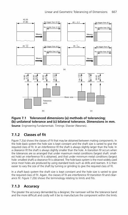
Linear and Geometric Tolerancing of Dimensions 667
7.1.2 Classes of fit
Figure 7.2(a) shows the classes of fit that may be obtained between mating components. Inthe hole basis system the hole size is kept constant and the shaft size is varied to give therequired class of fit. In an interference fit the shaft is always slightly larger than the hole. Ina clearance fit the shaft is always slightly smaller than the hole. A transition fit occurs whenthe tolerances are so arranged that under maximum metal conditions (largest shaft: small-est hole) an interference fit is obtained, and that under minimum metal conditions (largesthole: smallest shaft) a clearance fit is obtained. The hole basis system is the most widely usedsince most holes are produced by using standard tools such as drills and reamers. It is theneasier to vary the size of the shaft by turning or grinding to give the required class of fit.
In a shaft basis system the shaft size is kept constant and the hole size is varied to give the required class of fit. Again, the classes of fit are interference fit transition fit and clear-ance fit. Figure 7.2(b) shows the terminology relating to limits and fits.
7.1.3 Accuracy
The greater the accuracy demanded by a designer, the narrower will be the tolerance bandand the more difficult and costly will it be to manufacture the component within the limits
Basic size
Tolerancezone
(b)
(a)
(c)
19.
95�
0.10
20.0
019
.90
20.
00�
0.10
20�
0.05
20.0
219
.92
20�
0.15
�0.
05
20�
0.08
�0.
02
45 �0.3�0.2 35 0
�0.05
42.2541.80 No bigger than 42.25 No bigger than 40.140 � 0.1
No smaller than 41.80
No bigger than 45.3
No smaller than 44.8
No bigger than 35
No smaller than 34.95
No smaller than 39.9
MeansMeans
MeansMeans
Figure 7.1 Toleranced dimensions (a) methods of tolerancing; (b) unilateral tolerance and (c) bilateral tolerance. Dimensions in mm.Source: Engineering Fundamentals: Timings: Elsevier (Newnes).
H6508-Ch07.qxd 9/12/05 4:53 PM Page 667
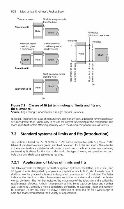
specified. Therefore, for ease of manufacture at minimum cost, a designer never specifies anaccuracy greater than is necessary to ensure the correct functioning of the component. Themore important factors affecting accuracy when measuring components are as follows.
7.2 Standard systems of limits and fits (introduction)
This section is based on BS EN 20286-2: 1993 and is compatible with ISO 286-2: 1988tables of standard tolerance grades and limit deviations for holes and shafts. These tablesin these standards are suitable for all classes of work from the finest instruments to heavyengineering. It allows for the size of the work, the type of work, and provides for bothhole basis and shaft basis systems as required.
7.2.1 Application of tables of limits and fits
The tables provide for 28 types of shaft designated by lower-case letters, a, b, c, etc., and28 types of hole designated by upper-case (capital) letters A, B, C, etc. To each type ofshaft or hole the grade of tolerance is designated by a number 1–18 inclusive. The letterindicates the position of the tolerance relative to the basic size and is called the funda-mental deviation. The number indicates the magnitude of the tolerance and is called thefundamental tolerance. A shaft is completely defined by its basic size, letter and number(e.g. 75 mm h6). Similarly a hole is completely defined by its basic size, letter and number,for example: 75 mm H7. Table 7.1 shows a selection of limits and fits for a wide range ofhole and shaft combinations for a variety of applications.
668 Mechanical Engineer’s Pocket Book
Shaft is always smallerthan the hole
Tolerance zone
Clearance fit
Transition fit
Interference fit
Hole
Hole
Hole
Hole
Shaft
Shaft
Shaft
Shaft
Shaft
Minimum metalcondition givesa clearance fit
Maximum metalcondition gives aninterference fit
Shaft is always largerthan the hole
(a)
Upp
er li
mit
of s
ize
Low
er li
mit
of s
ize
Allowance(Minimum clearance)
Tolerance
Low
er li
mit
of s
ize
Upp
er li
mit
of s
ize
Tolerance
(b)
Figure 7.2 Classes of fit (a) terminology of limits and fits and (b) allowance.Source: Engineering Fundamentals: Timings: Elsevier (Newnes).
H6508-Ch07.qxd 9/12/05 4:53 PM Page 668
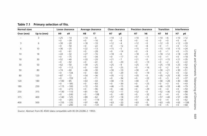
Linear and Geom
etric Tolerancing of Dim
ensions669
Table 7.1 Primary selection of fits.
Normal sizes Loose clearance Average clearance Close clearance Precision clearance Transition Interference
Over (mm) Up to (mm) H9 e9 H8 f7 H7 g6 H7 h6 H7 k6 H7 p6
– 3 �25 �14 �14 �6 �10 �2 �10 �0 �10 �6 �10 �12�0 �39 �0 �16 �0 �8 �0 �6 �0 �0 �0 �6
3 6 �30 �20 �18 �10 �12 �4 �12 �0 �12 �9 �12 �20�0 �50 �0 �22 �0 �12 �0 �8 �0 �1 �0 �12
6 10 �36 �25 �22 �13 �15 �5 �15 �0 �15 �10 �15 �24�0 �61 �0 �28 �0 �14 �0 �9 �0 �1 �0 �15
10 18 �43 �32 �27 �16 �18 �6 �18 �0 �18 �12 �18 �29�0 �75 �0 �34 �0 �17 �0 �11 �0 �1 �0 �18
18 30 �52 �40 �33 �20 �21 �7 �21 �0 �21 �15 �21 �35�0 �92 �0 �41 �0 �20 �0 �13 �0 �2 �0 �22
30 50 �62 �50 �39 �25 �25 �9 �25 �0 �25 �18 �25 �42�0 �112 �0 �50 �0 �25 �0 �16 �0 �2 �0 �26
50 80 �74 �60 �46 �30 �30 �10 �30 �0 �30 �21 �30 �51�0 �134 �0 �60 �0 �29 �0 �19 �0 �2 �0 �32
80 120 �87 �72 �54 �36 �35 �12 �35 �0 �35 �25 �35 �59�0 �159 �0 �71 �0 �34 �0 �22 �0 �3 �0 �37
120 180 �100 �85 �63 �43 �40 �14 �40 �0 �40 �28 �40 �68�0 �185 �0 �83 �0 �39 �0 �25 �0 �3 �0 �43
180 250 �115 �100 �72 �50 �46 �15 �46 �0 �46 �33 �46 �79�0 �215 �0 �96 �0 �44 �0 �29 �0 �4 �0 �50
250 315 �130 �110 �81 �56 �52 �17 �52 �0 �52 �36 �52 �88�0 �240 �0 �108 �0 �49 �0 �32 �0 �4 �0 �56
315 400 �140 �125 �89 �62 �57 �18 �57 �0 �57 �40 �57 �98�0 �265 �0 �119 �0 �54 �0 �36 �0 �4 �0 �62
400 500 �155 �135 �97 �68 �63 �20 �63 �0 �63 �45 �63 �108�0 �290 �0 �131 �0 �60 �0 �40 �0 �5 �0 �68
Source: Abstract from BS 4500 (data compatible with BS EN 20286-2: 1993).
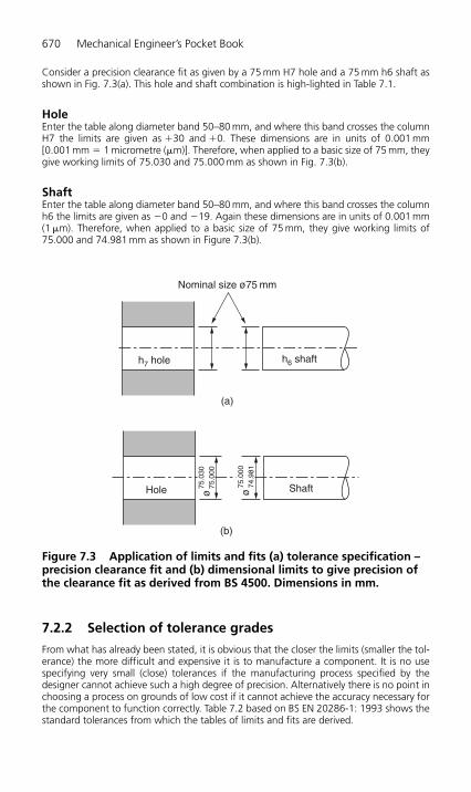
670 Mechanical Engineer’s Pocket Book
Consider a precision clearance fit as given by a 75 mm H7 hole and a 75 mm h6 shaft asshown in Fig. 7.3(a). This hole and shaft combination is high-lighted in Table 7.1.
HoleEnter the table along diameter band 50–80 mm, and where this band crosses the columnH7 the limits are given as �30 and �0. These dimensions are in units of 0.001 mm[0.001 mm � 1 micrometre (�m)]. Therefore, when applied to a basic size of 75 mm, theygive working limits of 75.030 and 75.000 mm as shown in Fig. 7.3(b).
ShaftEnter the table along diameter band 50–80 mm, and where this band crosses the columnh6 the limits are given as �0 and �19. Again these dimensions are in units of 0.001 mm(1 �m). Therefore, when applied to a basic size of 75 mm, they give working limits of75.000 and 74.981 mm as shown in Figure 7.3(b).
Nominal size ø75 mm
h7 hole h6 shaft
(a)
ShaftHole ø75
.030
75.0
00
ø75
.000
74.9
81
(b)
Figure 7.3 Application of limits and fits (a) tolerance specification –precision clearance fit and (b) dimensional limits to give precision ofthe clearance fit as derived from BS 4500. Dimensions in mm.
7.2.2 Selection of tolerance grades
From what has already been stated, it is obvious that the closer the limits (smaller the tol-erance) the more difficult and expensive it is to manufacture a component. It is no usespecifying very small (close) tolerances if the manufacturing process specified by thedesigner cannot achieve such a high degree of precision. Alternatively there is no point inchoosing a process on grounds of low cost if it cannot achieve the accuracy necessary forthe component to function correctly. Table 7.2 based on BS EN 20286-1: 1993 shows thestandard tolerances from which the tables of limits and fits are derived.
H6508-Ch07.qxd 9/12/05 4:53 PM Page 670
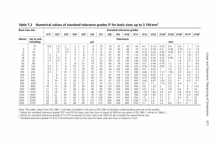
Linear and Geom
etric Tolerancing of Dim
ensions671
Table 7.2 Numerical values of standard tolerance grades IT for basic sizes up to 3 150 mm1
Basic size mm Standard tolerance grades
IT12 IT22 IT32 IT42 IT52 IT6 IT7 IT8 IT9 IT10 IT11 IT12 IT13 IT143 IT153 IT163 IT173 IT183
Above Up to and Tolerancesincluding �m mm
– 33 0.8 1.2 2 3 4 6 10 14 25 40 60 0.1 0.14 0.25 0.4 0.6 1 1.43 6 1 1.5 2.5 4 5 8 12 18 30 48 75 0.12 0.18 0.3 0.48 0.75 1.2 1.86 10 1 1.5 2.5 4 6 9 15 22 36 58 90 0.15 0.22 0.36 0.58 0.9 1.5 2.2
10 18 1.2 2 3 5 8 11 18 27 43 70 110 0.18 0.27 0.43 0.7 1.1 1.8 2.718 30 1.5 2.5 4 6 9 13 21 33 52 84 130 0.21 0.33 0.52 0.84 1.3 2.1 3.330 50 1.5 2.5 4 7 11 16 25 39 62 100 160 0.25 0.39 0.62 1 1.6 2.5 3.950 80 2 3 5 8 13 19 30 46 74 120 190 0.3 0.46 0.74 1.2 1.9 3 4.680 120 2.5 4 6 10 15 22 35 54 87 140 220 0.35 0.54 0.87 1.4 2.2 3.5 5.4
120 180 3.5 5 8 12 18 25 40 63 100 160 250 0.4 0.63 1 1.6 2.5 4 6.3180 250 4.5 7 10 14 20 29 46 72 115 185 290 0.46 0.72 1.15 1.85 2.9 4.6 7.2250 315 6 8 12 16 23 32 52 81 130 210 320 0.52 0.81 1.3 2.1 3.2 5.2 8.1315 400 7 9 13 18 25 36 57 89 140 230 360 0.57 0.89 1.4 2.3 3.6 5.7 8.9400 500 8 10 15 20 27 40 63 97 155 250 400 0.63 0.97 1.55 2.5 4 6.3 9.7500 6302 9 11 16 22 32 44 70 110 175 280 440 0.7 1.1 1.75 2.8 4.4 7 11630 8002 10 13 18 25 36 50 80 125 200 320 500 0.8 1.25 2 3.2 5 8 12.5800 10002 11 15 21 28 40 56 90 140 230 360 560 0.9 1.4 2.3 3.6 5.6 9 14
1000 12502 13 18 24 33 47 66 105 165 260 420 660 1.05 1.65 2.6 4.2 6.6 10.5 16.51250 16002 15 21 29 39 55 78 125 195 310 500 780 1.25 1.95 3.1 5 7.8 12.5 19.51600 20002 18 25 35 46 65 92 150 230 370 600 920 1.5 2.3 3.7 6 9.2 15 232000 25002 22 30 41 55 78 110 175 280 440 700 1100 1.75 2.8 4.4 7 11 17.5 282500 31502 26 36 50 68 96 135 210 330 540 860 1350 2.1 3.3 5.4 8.6 13.5 21 33
Note: This table, taken from ISO 286-1, has been included in this part of ISO 286 to facilitate understanding and use of the system.1 Values for standard tolerance grades IT01 and IT0 for basic sizes less than or equal to 500 mm are given in ISO 286-1, Annex A, Table 5.2 Values for standard tolerance grades IT1 to IT5 (inclusive) for basic sizes over 500 mm are included for experimental use.3 Standard tolerance grades IT14 to IT18 (inclusive) shall not be used for basic sizes less than or equal to 1 mm.
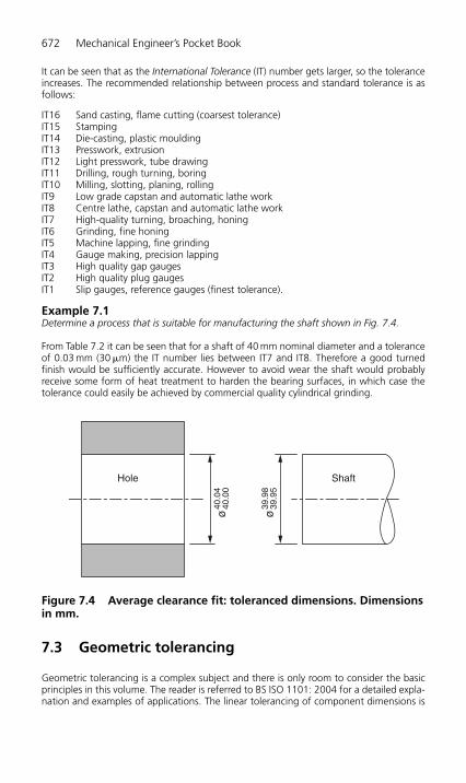
672 Mechanical Engineer’s Pocket Book
It can be seen that as the International Tolerance (IT) number gets larger, so the toleranceincreases. The recommended relationship between process and standard tolerance is asfollows:
IT16 Sand casting, flame cutting (coarsest tolerance)IT15 StampingIT14 Die-casting, plastic mouldingIT13 Presswork, extrusionIT12 Light presswork, tube drawingIT11 Drilling, rough turning, boringIT10 Milling, slotting, planing, rollingIT9 Low grade capstan and automatic lathe workIT8 Centre lathe, capstan and automatic lathe workIT7 High-quality turning, broaching, honingIT6 Grinding, fine honingIT5 Machine lapping, fine grindingIT4 Gauge making, precision lappingIT3 High quality gap gaugesIT2 High quality plug gaugesIT1 Slip gauges, reference gauges (finest tolerance).
Example 7.1Determine a process that is suitable for manufacturing the shaft shown in Fig. 7.4.
From Table 7.2 it can be seen that for a shaft of 40 mm nominal diameter and a toleranceof 0.03 mm (30 �m) the IT number lies between IT7 and IT8. Therefore a good turned finish would be sufficiently accurate. However to avoid wear the shaft would probablyreceive some form of heat treatment to harden the bearing surfaces, in which case thetolerance could easily be achieved by commercial quality cylindrical grinding.
Hole Shaft
ø40
.04
40.0
0
ø39
.98
39.9
5
Figure 7.4 Average clearance fit: toleranced dimensions. Dimensionsin mm.
7.3 Geometric tolerancing
Geometric tolerancing is a complex subject and there is only room to consider the basicprinciples in this volume. The reader is referred to BS ISO 1101: 2004 for a detailed expla-nation and examples of applications. The linear tolerancing of component dimensions is
H6508-Ch07.qxd 9/12/05 4:53 PM Page 672
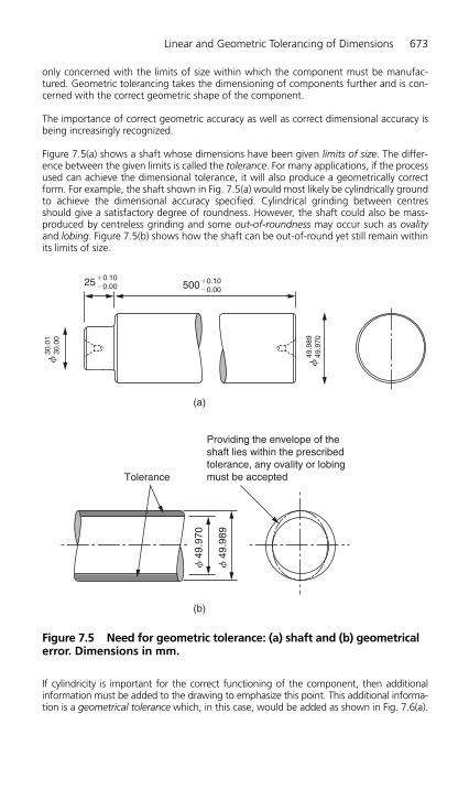
Linear and Geometric Tolerancing of Dimensions 673
only concerned with the limits of size within which the component must be manufac-tured. Geometric tolerancing takes the dimensioning of components further and is con-cerned with the correct geometric shape of the component.
The importance of correct geometric accuracy as well as correct dimensional accuracy isbeing increasingly recognized.
Figure 7.5(a) shows a shaft whose dimensions have been given limits of size. The differ-ence between the given limits is called the tolerance. For many applications, if the processused can achieve the dimensional tolerance, it will also produce a geometrically correctform. For example, the shaft shown in Fig. 7.5(a) would most likely be cylindrically groundto achieve the dimensional accuracy specified. Cylindrical grinding between centresshould give a satisfactory degree of roundness. However, the shaft could also be mass-produced by centreless grinding and some out-of-roundness may occur such as ovalityand lobing. Figure 7.5(b) shows how the shaft can be out-of-round yet still remain withinits limits of size.
25 �0.10�0.00
f30
.01
30.0
0
f49
.989
49.9
70
f 4
9.97
0
f 4
9.98
9
500
(a)
(b)
Providing the envelope of theshaft lies within the prescribedtolerance, any ovality or lobingmust be acceptedTolerance
�0.10�0.00
Figure 7.5 Need for geometric tolerance: (a) shaft and (b) geometricalerror. Dimensions in mm.
If cylindricity is important for the correct functioning of the component, then additionalinformation must be added to the drawing to emphasize this point. This additional informa-tion is a geometrical tolerance which, in this case, would be added as shown in Fig. 7.6(a).
H6508-Ch07.qxd 9/12/05 4:53 PM Page 673
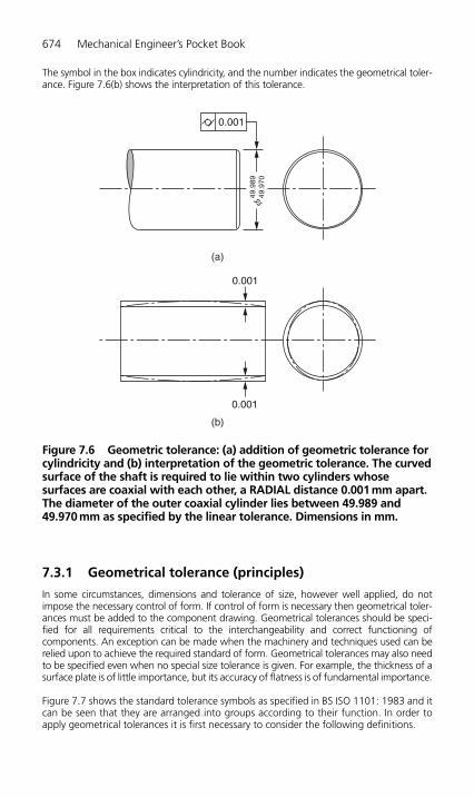
674 Mechanical Engineer’s Pocket Book
The symbol in the box indicates cylindricity, and the number indicates the geometrical toler-ance. Figure 7.6(b) shows the interpretation of this tolerance.
f49
.989
49.9
70
0.001
0.001
0.001
(a)
(b)
Figure 7.6 Geometric tolerance: (a) addition of geometric tolerance forcylindricity and (b) interpretation of the geometric tolerance. The curvedsurface of the shaft is required to lie within two cylinders whose surfaces are coaxial with each other, a RADIAL distance 0.001 mm apart.The diameter of the outer coaxial cylinder lies between 49.989 and49.970 mm as specified by the linear tolerance. Dimensions in mm.
7.3.1 Geometrical tolerance (principles)
In some circumstances, dimensions and tolerance of size, however well applied, do notimpose the necessary control of form. If control of form is necessary then geometrical toler-ances must be added to the component drawing. Geometrical tolerances should be speci-fied for all requirements critical to the interchangeability and correct functioning ofcomponents. An exception can be made when the machinery and techniques used can berelied upon to achieve the required standard of form. Geometrical tolerances may also needto be specified even when no special size tolerance is given. For example, the thickness of asurface plate is of little importance, but its accuracy of flatness is of fundamental importance.
Figure 7.7 shows the standard tolerance symbols as specified in BS ISO 1101: 1983 and itcan be seen that they are arranged into groups according to their function. In order toapply geometrical tolerances it is first necessary to consider the following definitions.
H6508-Ch07.qxd 9/12/05 4:53 PM Page 674
Linear and Geom
etric Tolerancing of Dim
ensions675
Features and tolerances Toleranced characteristics Symbols Subclauses
Straightness 14.1
14.2
14.3
14.4
14.5
14.6
14.7
14.8
14.9
14.10
14.11
14.12
14.13
14.14
Flatness
Circularity
Cylindricity
Profile of any line
Profile of any surface
Parallelism
Perpendicularity
Angularity
Position
Concentricity and coaxiality
Symmetry
Circular run-out
Total run-out
Form tolerances
Orientation tolerances
Location tolerances
Run-out tolerances
Single features
Single or related features
Related features
Figure 7.7 Geometrical tolerancing symbols (a) symbols for toleranced characteristics.
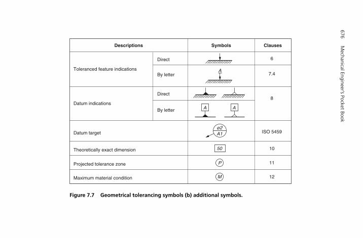
676M
echanical Engineer’s Pocket Book
Descriptions
Direct
Direct
By letter
By letter
Toleranced feature indications
Datum indications
Datum target
Theoretically exact dimension
Projected tolerance zone
Maximum material condition
Symbols
A
A
Clauses
6
8
10
11
12
ISO 5459
7.4
A
A1ø2
50
P
M
Figure 7.7 Geometrical tolerancing symbols (b) additional symbols.
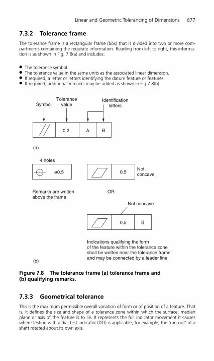
Linear and Geometric Tolerancing of Dimensions 677
7.3.2 Tolerance frame
The tolerance frame is a rectangular frame (box) that is divided into two or more com-partments containing the requisite information. Reading from left to right, this informa-tion is as shown in Fig. 7.8(a) and includes:
● The tolerance symbol.● The tolerance value in the same units as the associated linear dimension.● If required, a letter or letters identifying the datum feature or features.● If required, additional remarks may be added as shown in Fig.7.8(b).
Symbol
4 holes
Remarks are writtenabove the frame
OR
Notconcave
Not concave
Indications qualifying the formof the feature within the tolerance zoneshall be written near the tolerance frameand may be connected by a leader line.
(a)
(b)
Tolerancevalue
Identificationletters
0.2
ø0.5
A B
0.5
0.5 B
Figure 7.8 The tolerance frame (a) tolerance frame and (b) qualifying remarks.
7.3.3 Geometrical tolerance
This is the maximum permissible overall variation of form or of position of a feature. Thatis, it defines the size and shape of a tolerance zone within which the surface, medianplane or axis of the feature is to lie. It represents the full indicator movement it causeswhere testing with a dial test indicator (DTI) is applicable, for example, the ‘run-out’ of ashaft rotated about its own axis.
H6508-Ch07.qxd 9/12/05 4:53 PM Page 677

678 Mechanical Engineer’s Pocket Book
7.3.4 Tolerance zone
This is the zone within which the feature has to be contained. Thus, according to thecharacteristic that is to be toleranced and the manner in which it is to be dimensioned,the tolerance zone is one of the following:
● A circle or a cylinder.● The area between two parallel lines or two parallel straight lines.● The space between two parallel surfaces or two parallel planes.● The space within a parallelepiped.
NoteThe tolerance zone, once established, permits any feature to vary within that zone. If it isconsidered necessary to prohibit sudden changes in surface direction, or to control therate of change of a surface within this zone, this should be additionally specified.
7.3.5 Geometrical reference frame
This is the diagram composed of the constructional dimensions that serve to establish thetrue geometrical relationships between positional features in any one group as shown inFig. 7.9. For example, the symbol indicates that the hole centre may lie anywhere withina circle of 0.02 mm diameter that is itself centred upon the intersection of the frame. Thedimension indicates that the reference frame is a geometrically perfect square of sidelength 40 mm.
ø0.02
ø0.02 Tolerance zone(centre of hole A may lieanywhere within or onthe circumference of thiscircle)
Geometric reference frame(a perfect geometric squareof 40 mm side)
4 holesø6 H12
A A
A
15.515.0 15
.515
.0
40
(a) (b)
A
40
40
40
Figure 7.9 The geometric tolerance diagram (a) drawing requirementand (b) reference frame. Dimensions in mm.
H6508-Ch07.qxd 9/12/05 4:53 PM Page 678
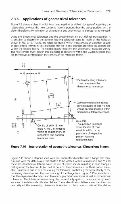
Linear and Geometric Tolerancing of Dimensions 679
7.3.6 Applications of geometrical tolerances
Figure 7.9 shows a plate in which four holes need to be drilled. For ease of assembly, therelationship between the hole-centres is more important than the group position on theplate. Therefore a combination of dimensional and geometrical tolerances has to be used.
Using the dimensional tolerances and the boxed dimension that defines true position, itis possible to determine the pattern locating tolerance zone for each of the holes asshown in Fig. 7.10. That is, the reference frame (which must always by a perfect squareof side length 40 mm in this example) may lie in any position providing its corners arewithin the shaded boxes. The shaded boxes represent the dimensional tolerance zones.The hole centres may then (in this example) lie anywhere within the 0.02 mm circles thatare themselves centred upon the corners of the reference frame.
40
Pattern locating tolerancezone determined bydimensional tolerances
Geometric tolerance frame:perfect square of side 40 mmwhose corners must lie withindimensional tolerance zones
ø0.2 mm –True position tolerancezone. Centre of zonemust lie within, or onperiphery of respectivepattern locatingtolerance zone
Centre of ø6 H12 hole(hole A, fig. 7.5) must liewithin or on periphery ofrespective true positiontolerance zone
40
40
40
15.5
0.25
0.25
0.25
15.5
15.0
0.25
15.0
Figure 7.10 Interpretation of geometric tolerances. Dimensions in mm.
Figure 7.11 shows a stepped shaft with four concentric diameters and a flange that mustrun true with the datum axis. The shaft is to be located within journals at X and Y, andthese are identified as datums. Note the use of leader lines terminating in solid trianglesresting upon the features to be used as datums. The common axis of these datum diam-eters is used as a datum axis for relating the tolerances controlling the concentricity of theremaining diameters and the true running of the flange face. Figure 7.11(a) also showsthat the dependent diameters and face carry geometric tolerances as well as dimensionaltolerances. The tolerance frames carry the concentricity symbol, the concentricity toler-ance and the datum identification letters. These identification letters show that the con-centricity of the remaining diameters is relative to the common axis of the datum
H6508-Ch07.qxd 9/12/05 4:53 PM Page 679
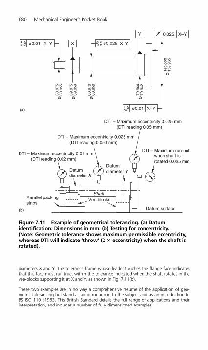
680 Mechanical Engineer’s Pocket Book
diameters X and Y. The tolerance frame whose leader touches the flange face indicatesthat this face must run true, within the tolerance indicated when the shaft rotates in thevee-blocks supporting it at X and Y, as shown in Fig. 7.11(b).
These two examples are in no way a comprehensive resume of the application of geo-metric tolerancing but stand as an introduction to the subject and as an introduction toBS ISO 1101:1983. This British Standard details the full range of applications and theirinterpretation, and includes a number of fully dimensioned examples.
ø0.01 X–Y X ø0.025 X–Y
ø0.01 X–Y
0.025 X–YY
ø30
.975
30.9
55
ø39
.975
39.9
59
ø60
.970
60.9
50
ø79
.964
79.9
42
ø16
0.00
015
9.96
5
(a)
DTI – Maximum eccentricity 0.025 mm (DTI reading 0.05 mm)
DTI – Maximum run-out when shaft is rotated 0.025 mm
Datum surface
Datumdiameter YDatum
diameter X
Parallel packingstrips
ShaftVee blocks
DTI – Maximum eccentricity 0.025 mm (DTI reading 0.050 mm)
DTI – Maximum eccentricity 0.01 mm (DTI reading 0.02 mm)
(b)
Figure 7.11 Example of geometrical tolerancing. (a) Datum identification. Dimensions in mm. (b) Testing for concentricity. (Note: Geometric tolerance shows maximum permissible eccentricity,whereas DTI will indicate ‘throw’ (2 � eccentricity) when the shaft isrotated).
H6508-Ch07.qxd 9/12/05 4:53 PM Page 680
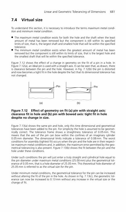
Linear and Geometric Tolerancing of Dimensions 681
7.4 Virtual size
To understand this section, it is necessary to introduce the terms maximum metal condi-tion and minimum metal condition.
● The maximum metal condition exists for both the hole and the shaft when the leastamount of metal has been removed but the component is still within its specified limits of size, that is, the largest shaft and smallest hole that will lie within the specifiedtolerance.
● The minimum metal condition exists when the greatest amount of metal has beenremoved but the component is still within its limits of size, that is the largest hole andthe smallest shaft that will lie within the specified tolerance.
Figure 7.12 shows the effect of a change in geometry on the fit of a pin in a hole. InFigure 7.12(a), an ideal pin is used with a straight axis. It can be seen that, as drawn, thereis clearance between the pin and the hole. However, in Fig. 7.12(b) the pin is distortedand now becomes a tight fit in the hole despite the fact that its dimensional tolerance hasnot changed.
Figure 7.13(a) shows the same pin and hole, only this time dimensional and geometricaltolerances have been added to the pin. For simplicity the hole is assumed to be geomet-rically correct. The tolerance frame shows a straightness tolerance of 0.05 mm. Thismeans that the axis of the pin can bow within the confines of an imaginary cylinder0.05 mm diameter. The dimensional limits indicate a tolerance of 0.08 mm. The worstconditions for assembly (tightest fit) occurs when the pin and the hole are in their respect-ive maximum metal conditions and, in addition, the maximum error permitted by the geo-metrical tolerancing is also present. Figure 7.13(b) shows the fit between the pin and thehole under these conditions.
Under such conditions the pin will just enter a truly straight and cylindrical hole equal tothe pin diameter under maximum metal conditions (25.00 mm) plus the geometrical tol-erance of 0.05 mm, that is a hole diameter of 25.05 mm. This theoretical hole diameter of25.05 mm is referred to as the virtual size for the pin.
Under minimum metal conditions, the geometrical tolerance for the pin can be increasedwithout altering the fit of the pin in the hole. As shown in Fig. 7.13(c), the geometric tol-erance can now be increased to 0.13 mm without any increase in the virtual size or thechange of fit.
Pin
(a) (b)
Pin
Figure 7.12 Effect of geometry on fit (a) pin with straight axis: clearance fit in hole and (b) pin with bowed axis: tight fit in holedespite no change in size.
H6508-Ch07.qxd 9/12/05 4:53 PM Page 681
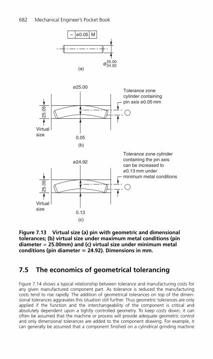
682 Mechanical Engineer’s Pocket Book
7.5 The economics of geometrical tolerancing
Figure 7.14 shows a typical relationship between tolerance and manufacturing costs forany given manufactured component part. As tolerance is reduced the manufacturingcosts tend to rise rapidly. The addition of geometrical tolerances on top of the dimen-sional tolerances aggravates this situation still further. Thus geometric tolerances are onlyapplied if the function and the interchangeability of the component is critical andabsolutely dependent upon a tightly controlled geometry. To keep costs down, it canoften be assumed that the machine or process will provide adequate geometric controland only dimensional tolerances are added to the component drawing. For example, itcan generally be assumed that a component finished on a cylindrical grinding machine
– ø0.05
(a)
(b)
(c)
ø25.0024.92
ø25.00
ø24.92
Tolerance zonecylinder containingpin axis ø0.05 mm
Tolerance zone cylindercontaining the pin axiscan be increased toø0.13 mm underminimum metal conditions
0.05
0.13
Virtualsize
Virtualsize
25.0
5
M
25.0
5
Figure 7.13 Virtual size (a) pin with geometric and dimensional tolerances; (b) virtual size under maximum metal conditions (pindiameter � 25.00mm) and (c) virtual size under minimum metal conditions (pin diameter � 24.92). Dimensions in mm.
H6508-Ch07.qxd 9/12/05 4:53 PM Page 682

between centres will be straight and cylindrical to a high degree of geometrical accuracy.However, current trends in quality control and just-in-time (JIT) scheduling tends toincrease the demand for closer dimensional and geometrical control to ensure no holdups occur during assembly and that any quality specifications are met first time withoutthe need for corrective action or rejection by the customer.
Linear and Geometric Tolerancing of Dimensions 683
Uni
t pro
duct
ion
cost
Combined tolerancingGeometric tolerance
Tolerance0
Dimensional tolerancing
Figure 7.14 Cost of tolerancing.
H6508-Ch07.qxd 9/12/05 4:53 PM Page 683

8Computer-Aided Engineering
8.1 Computer numerical control
8.1.1 Typical applications of computer numerical control
Computer numerical control (CNC) is applied to a wide range of production processes inmany industries. In the engineering industries it is applied to such processes as:
(a) Machine tools, including– Milling machines and machining centres– Centre lathes and turning centres– Drilling machines– Precision, grinding machines– Electro-discharge machining (EDM) (spark erosion) machines– Die sinking machines
(b) Sheet metal working machines, including– Turret punching machines– Riveting machines– Forming machines
(c) Fabrication equipment, including– Flame cutting machines– Welding machines– Tube bending machines
(d) Inspection machines for checking three-dimensionally (3D) contoured components.
8.1.2 Advantages and limitations of CNC
It is evident from the wide and increasing use of computer numerically controlledmachines in manufacturing industry that the advantages substantially outweigh the limitations.
AdvantagesHigh productivity Although the cutting speeds and feeds for CNC machines are thesame as for manually operated machines, much time is saved by rapid traversing and pos-itioning between operations. Also a wider range of operations is possible on a CNCmachine, avoiding the necessity to pass the work from one machine to another for, say,each of drilling, milling and boring. This reduces the need for expensive jigs and fixtures,and avoids reserves of work in progress between operations. In addition, CNC machinesdo not become tired and they maintain a constant rate of productivity. If the work is robotfed, they can work ‘lights out’ through the night.
H6508-Ch08.qxd 9/12/05 4:52 PM Page 684

Computer-Aided Engineering 685
Design flexibility Complex shapes are easily produced on CNC machines. In addition,contoured solids can be produced on CNC machines which cannot be produced on con-ventional, manually operated machines.
Management control Production rates, reduced scrap and improved quality comesunder management control with CNC machines and is not influenced by operator performance.
Quality CNC machines have a higher accuracy and better repeatability than conven-tional machines. If the machine is fitted with adaptive control it will even sense tool fail-ure or other variations in performance and either stop the machine or, if fitted withautomatic tool changing, select backup tooling from the tool magazine before scrap isproduced or the machine damaged.
Reduced lead time The lead time for CNC machines is much less than for other auto-matic machines. There are no complex and expensive cams and form tools; it is necessarysimply to write a part program and load it into the machine memory. Complex profiles aregenerated using standard tooling.
LimitationsCapital cost The initial cost of CNC machines is substantially higher than for manuallyoperated machines of the same type. However, in recent years, the cost differential hascome down somewhat.
Tooling cost To exploit the production potential of CNC machine tools, specialized cut-ting tools are required. Although the initial cost is high, this largely reflects the cost of thetool shanks and tool holding devices which do not have to be replaced. The cost ofreplacement tool tips is no higher than for conventional machines.
Maintenance Due to the complexity of CNC machine tools, few small and mediumcompanies will have the expertise to carry out more than very basic maintenance andrepairs. Therefore, maintenance contracts are advisable. These are expensive, approxi-mately 10% of the capital cost per annum.
Training Programmer/operator training is required. This is usually provided by theequipment manufacturer but can be time consuming and costly.
Depreciation As with all computer-based devices, CNC controllers rapidly becomeobsolescent. Therefore, CNC machines should be amortized over a shorter period than is usual with manually operated machines and should be replaced approximately every 5 years.
8.1.3 Axes of control for machine tools
There are a number of axis configurations for CNC machine tools; the most common areused with vertical/horizontal milling machines and lathes as shown. Note that:
(a) The Z-axis is always the main spindle axis.(b) The X-axis is always horizontal and perpendicular to the Z-axis.(c) The Y-axis is perpendicular to both the X- and Z-axis.
H6508-Ch08.qxd 9/12/05 4:52 PM Page 685
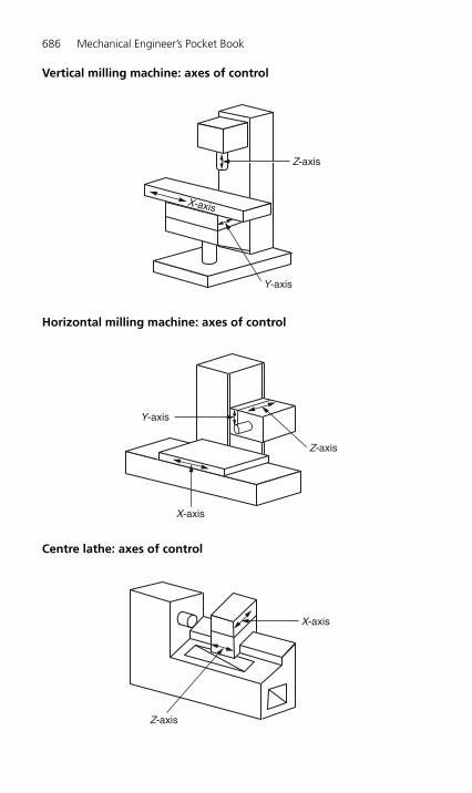
686 Mechanical Engineer’s Pocket Book
Vertical milling machine: axes of control
Z-axis
Y-axis
X-axis
Horizontal milling machine: axes of control
Z-axis
Y-axis
X-axis
Centre lathe: axes of control
Z-axis
X-axis
H6508-Ch08.qxd 9/12/05 4:52 PM Page 686

Computer-Aided Engineering 687
8.1.4 Control systems
Control systems for CNC machine tools broadly fall into two categories as follows.
Open-loop controlThis system derives its name from the fact that there is no feedback in the system, andhence no comparison between input and output. The system uses stepper motors to drivethe positioning mechanism, and these have only limited torque compared with more con-ventional servo motors. Further, if the drag of the mechanism causes the motor to stalland miss a step, no corrective action is taken by the system.
Inputsignal
Convertedsignal
Inputdevice
Manual data inputPunch paper tapeMagnetic tape
Controlsystem Amplifier
Control unitM/C tool slide
Output
Closed-loop controlThe following figure explains closed-loop control system:
Input signal
Inputdevice
Controlsystem
Converted signal
Amplifier
Manual data inputPunch paper tapeMagnetic tape
Action Output
FeedbackMeasuring
device
Position measuringtransducer
Control unitM/C tool slide
H6508-Ch08.qxd 9/12/05 4:52 PM Page 687

688 Mechanical Engineer’s Pocket Book
In a closed-loop control system the feedback continuously influences the action of thecontroller and corrects any positional errors. This system allows the use of servo motors todrive the positioning mechanism, and these have a much higher torque than the steppermotors used with the open-loop control system.
8.1.5 Program terminology and format
CharacterA character is a number, letter or other symbol which is recognized by the controller. Anassociated group of characters makes a word.
WordA word is a group of characters which defines one complete element of information (e.g.N100). There are two types of word as follows.
Dimensional wordsThese are any words related to a linear dimension; that is, any word commencing with thecharacters X, Y, Z, I, J, K or any word in which these characters are inferred.
The letters X, Y, Z refer to dimensions parallel to the corresponding machine axes, asexplained in Section 8.1.3.
The letters I, J, K refer to arcs of circles. The start and finish positions of the arcs aredefined by X, Y, Z dimensions, whilst the centre of radius of the arc is defined using I, J, Kdimensions, with:
I dimensions corresponding to X dimensionsJ dimensions corresponding to Y dimensionsK dimensions corresponding to Z dimensions.
Current practice favours the use of the decimal point in specifying dimension words. Thus,a machine manual may stipulate that an X dimension word has the form X4, 3, whichmeans that the X dimension may have up to 4 digits in front of the decimal point and up to3 digits behind the decimal point. Some older systems, still widely in use, do not use the deci-mal point but use leading and trailing zeros; for example, 25.4 would be written 0025400.
Management wordsThese are any words which are not related to a dimension; that is, any word commencingwith the characters N, G, F, S, T, M or any word in which the above characters are inferred.Examples of management words may be as follows:
N4 Sequence number: the character N followed by up to four digits (i.e. N1 … N9999).G2 Preparatory function: the character G followed by up to two digits (i.e. G0 … G99).F4 Feed rate command: the character F followed by up to four digits.S4 Spindle speed command: the character S followed by up to four digits.T2 Tool identifier: the character T followed by up to two digits.M2 Miscellaneous commands: the character M followed by up to two digits.
Note that N, G, T and M commands may require leading zeros to be programmed onsome older but still widely used systems (e.g. G0 would be G00, G1 would be G01, etc.).
8.1.6 Word (or letter) address format
This is, currently, the most widely used format. Each word commences with a letter char-acter called an address. Hence, a word is identified by its letter character and not by itsposition in the block (in contrast to the fixed block system described below). Thus in a
H6508-Ch08.qxd 9/12/05 4:52 PM Page 688

Computer-Aided Engineering 689
word (or letter) address format, instructions which remain unchanged from a previousblock may be omitted from subsequent blocks.
A typical letter address format, as given by a maker’s handbook, could be:
Metric N4 G2 X4, 3 Y4, 3 Z4, 3 I4, 3 J4, 3 K4, 3 F3 S4 T2 M2Inch N4 G2 X3, 4 Y3, 4 Z3, 4 I3, 4 J3, 4 K3, 4 F3 S4 T2 M2
8.1.7 Coded information
A CNC program contains the information for the manufacture of a component part. TheCNC controller regulates the signals and sequence to the various drive units.
CodesBlock numbers NPreparatory functions GDimensional data X, Y, Z, I, J, KFeed rates FSpindle speeds STool numbers TMiscellaneous functions M
A sample of a CNC program could look like this:
N5 G90 G71 G00 X25.0 Y25.0 T01 M06N10 X100.0 Y100.0 S1250N15 G01 Z25.0 F125 M03
Block numbersThe block number is usually the first word which appears in any block. Blocks are numberedin steps of 5 or 10 so that additional blocks can be easily inserted in the event of an omission.
Preparatory functions (G)These are used to inform the machine controller of the functions required for the nextoperation. Standardized preparatory functions are shown in the following table. In prac-tice, the actual codes used will depend on the control system and the machinetype. The codes that one system uses can vary from those of another, so refer-ence to the relevant programming manual is essential.
Code number Functiona
G00 Rapid positioning, point to point (M)G01 Positioning at controlled feed rate, normal dimensions (M)G02 Circular interpolation, normal dimensions (M)G03 Circular interpolation counter clockwise (CCW), normal dimensions (M)G04 Dwell for programmed durationG05 � Hold: cancelled by operatorG06 Reserved for future standardization: notG07 normally usedG08 Programmed slide accelerationG09 Programmed slide decelerationG10 Linear interpolation, long dimensions (M)G11 Linear interpolation, short dimensions (M)G12 3D interpolation (M)G13–G16 Axis selection (M)G17 XY plane selection (M)G18 ZX plane selection (M)G19 YZ plane selection (M)G20 Circular interpolation clockwise (CW), long dimensions (M)G21 Circular interpolation CW, short dimensions (M)
continued
H6508-Ch08.qxd 9/12/05 4:52 PM Page 689
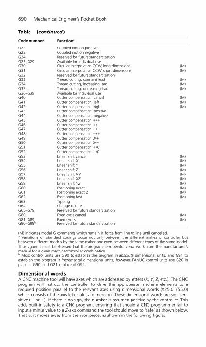
690 Mechanical Engineer’s Pocket Book
Table (continued )
Code number Functiona
G22 Coupled motion positiveG23 Coupled motion negativeG24 Reserved for future standardizationG25–G29 Available for individual useG30 Circular interpolation CCW, long dimensions (M)G31 Circular interpolation CCW, short dimensions (M)G32 Reserved for future standardizationG33 Thread cutting, constant lead (M)G34 Thread cutting, increasing lead (M)G35 Thread cutting, decreasing lead (M)G36–G39 Available for individual useG40 Cutter compensation, cancel (M)G41 Cutter compensation, left (M)G42 Cutter compensation, right (M)G43 Cutter compensation, positiveG44 Cutter compensation, negativeG45 Cutter compensation �/�G46 Cutter compensation �/�G47 Cutter compensation �/�G48 Cutter compensation �/�G49 Cutter compensation 0/�G50 Cutter compensation 0/�G51 Cutter compensation �/0G52 Cutter compensation �/0G53 Linear shift cancel (M)G54 Linear shift X (M)G55 Linear shift Y (M)G56 Linear shift Z (M)G57 Linear shift XY (M)G58 Linear shift XZ (M)G59 Linear shift YZ (M)G60 Positioning exact 1 (M)G61 Positioning exact 2 (M)G62 Positioning fast (M)G63 TappingG64 Change of rateG65–G79 Reserved for future standardizationG80 Fixed cycle cancel (M)G81–G89 Fixed cycles (M)G90–G99b Reserved for future standardization
(M) indicates modal G commands which remain in force from line to line until cancelled.a Variations on standard codings occur not only between the different makes of controller butbetween different models by the same maker and even between different types of the same model.Thus again it must be stressed that the programmer/operator must work from the manufacturer’smanual for a given machine/controller combination.b Most control units use G90 to establish the program in absolute dimensional units, and G91 toestablish the program in incremental dimensional units, however. FANUC control units use G20 inplace of G90, and G21 in place of G92.
Dimensional wordsA CNC machine tool will have axes which are addressed by letters (X, Y, Z, etc.). The CNCprogram will instruct the controller to drive the appropriate machine elements to arequired position parallel to the relevant axes using dimensional words (X25.0 Y55.0)which consists of the axis letter plus a dimension. These dimensional words are sign sen-sitive (� or �). If there is no sign, the number is assumed positive by the controller. Thisadds built-in safety to a CNC program, ensuring that should a CNC programmer fail toinput a minus value to a Z-axis command the tool should move to ‘safe’ as shown below.That is, it moves away from the workpiece, as shown in the following figure.
H6508-Ch08.qxd 9/12/05 4:52 PM Page 690

Computer-Aided Engineering 691
30
Tool retracts30 mm from datumif Z30 is programmed
Tool penetrateswork by 30 mmif Z-30.0 isprogrammed
30 Workpiece
ToolDirection of toolmovement alongZ-axis
Datumnormally Z0
�
�
Consider a line of program N10 G01 X25.0 Y25.0 Z30.0. This would result in the toolmoving to the coordinates X25, Y25, Z30. However, since the Z word is positive the toolwill go up and not down 30 mm from the datum. To drill the component to a depth of30 mm the line of program should read N10 G01 X25.0 Y25.0 Z-30.0.
Feed rate (F)Words commencing with F indicate to the controller the desired feed rate for machining.There are a number of ways of defining the feed rate:
(a) Millimetres/minute: F30 � 30 mm/min.(b) Millimetres/revolution: F0.2 � 0.2 mm/rev.(c) Feed rate number 1–20 indicates feed rates predetermined by the manufacture in
rev/min or mm/min as appropriate. To use this system the feed rate command is pref-aced by a G code. Only a few older machines use this system.
Spindle speed (S)Words commencing with the letter S indicate to the controller the desired spindle speedfor machining. Once again there are a number of ways of defining the spindle speed,each selected by use of the appropriate G code:
(a) Spindle speed in revolutions /minute (r.p.m.).(b) Cutting speed in metres /minute.(c) Constant cutting speed in metres /minute.
Tool numbers (T)Each tool used during the machining of a part will have its own number (e.g. T01 for tool1, T19 for tool 19). Most CNC machine controllers can hold information about 20 tools ormore. This tool information will take the form of a tool length offset (TLO) and a tool diam-eter/radius compensation (see Sections 8.1.9 and 8.1.10). Where the machine is fitted withautomatic tool changing it will also identify the position of the tool in the tool magazine.
Miscellaneous functions (M)Apart from preparatory functions there are a number of other functions that are requiredthroughout the program (e.g. ‘switch spindle on’, ‘switch coolant on’, etc). These func-tions have been standardized and are popularly known as M codes. The address letter Mis followed by two digits. The most commonly used M codes are as follows:
M00 Program stop M04 Spindle on CCW M08 Flood coolant onM01 Optional stop M05 Spindle off M09 Coolant offM02 End program M06 Tool change M30 End of tapeM03 Spindle on CW M07 Mist coolant on
H6508-Ch08.qxd 9/12/05 4:52 PM Page 691
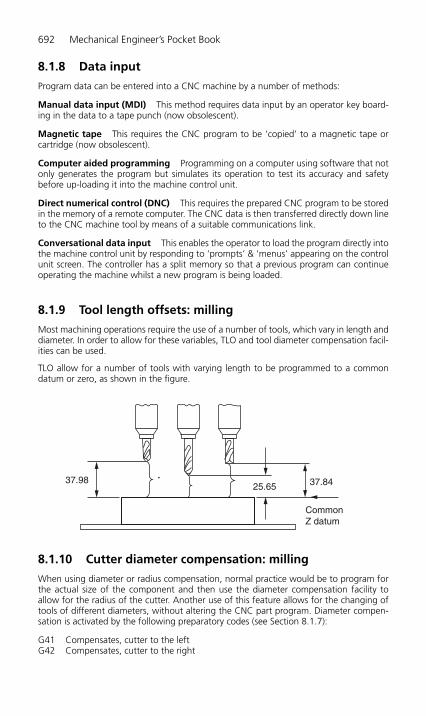
692 Mechanical Engineer’s Pocket Book
8.1.8 Data input
Program data can be entered into a CNC machine by a number of methods:
Manual data input (MDI) This method requires data input by an operator key board-ing in the data to a tape punch (now obsolescent).
Magnetic tape This requires the CNC program to be ‘copied’ to a magnetic tape orcartridge (now obsolescent).
Computer aided programming Programming on a computer using software that notonly generates the program but simulates its operation to test its accuracy and safetybefore up-loading it into the machine control unit.
Direct numerical control (DNC) This requires the prepared CNC program to be storedin the memory of a remote computer. The CNC data is then transferred directly down lineto the CNC machine tool by means of a suitable communications link.
Conversational data input This enables the operator to load the program directly intothe machine control unit by responding to ‘prompts’ & ‘menus’ appearing on the controlunit screen. The controller has a split memory so that a previous program can continueoperating the machine whilst a new program is being loaded.
8.1.9 Tool length offsets: milling
Most machining operations require the use of a number of tools, which vary in length anddiameter. In order to allow for these variables, TLO and tool diameter compensation facil-ities can be used.
TLO allow for a number of tools with varying length to be programmed to a commondatum or zero, as shown in the figure.
37.9825.65 37.84
CommonZ datum
8.1.10 Cutter diameter compensation: milling
When using diameter or radius compensation, normal practice would be to program forthe actual size of the component and then use the diameter compensation facility toallow for the radius of the cutter. Another use of this feature allows for the changing oftools of different diameters, without altering the CNC part program. Diameter compen-sation is activated by the following preparatory codes (see Section 8.1.7):
G41 Compensates, cutter to the leftG42 Compensates, cutter to the right
H6508-Ch08.qxd 9/12/05 4:52 PM Page 692

Computer-Aided Engineering 693
G41 Compensation to the leftThe cutter is always to the left of the surface being machined when looking along thepath of the cutter, as indicated by the arrows in the figure.
Direction of tool movement
Workpiece
Cutting tool
G41
G42 Compensation to the rightThe cutter is always to the right of the surface being machined when looking along thepath of the cutter, as indicated by the arrows in the figure.
Direction of tool movement
Workpiece
Cutting tool
G42
H6508-Ch08.qxd 9/12/05 4:52 PM Page 693
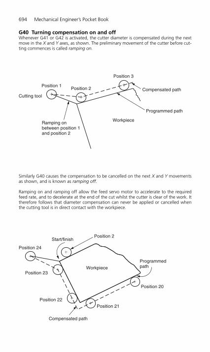
694 Mechanical Engineer’s Pocket Book
G40 Turning compensation on and offWhenever G41 or G42 is activated, the cutter diameter is compensated during the nextmove in the X and Y axes, as shown. The preliminary movement of the cutter before cut-ting commences is called ramping on.
Cutting tool ��
�Position 1Position 2
Position 3
Programmed path
Compensated path
Ramping onbetween position 1and position 2
Workpiece
Similarly G40 causes the compensation to be cancelled on the next X and Y movementsas shown, and is known as ramping off.
Ramping on and ramping off allow the feed servo motor to accelerate to the requiredfeed rate, and to decelerate at the end of the cut whilst the cutter is clear of the work. Ittherefore follows that diameter compensation can never be applied or cancelled whenthe cutting tool is in direct contact with the workpiece.
Position 24
Position 23
Position 22Position 21
Position 20
Position 2Start/finish
Programmedpath
Compensated path
Workpiece
�
��
�
��
H6508-Ch08.qxd 9/12/05 4:52 PM Page 694
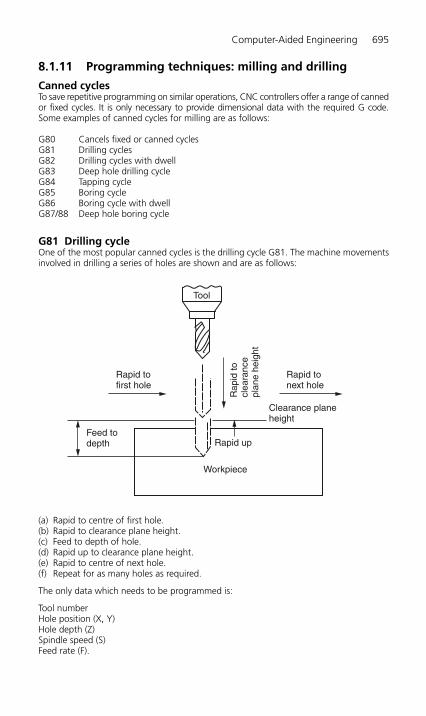
Computer-Aided Engineering 695
8.1.11 Programming techniques: milling and drilling
Canned cyclesTo save repetitive programming on similar operations, CNC controllers offer a range of cannedor fixed cycles. It is only necessary to provide dimensional data with the required G code.Some examples of canned cycles for milling are as follows:
G80 Cancels fixed or canned cyclesG81 Drilling cyclesG82 Drilling cycles with dwellG83 Deep hole drilling cycleG84 Tapping cycleG85 Boring cycleG86 Boring cycle with dwellG87/88 Deep hole boring cycle
G81 Drilling cycleOne of the most popular canned cycles is the drilling cycle G81. The machine movementsinvolved in drilling a series of holes are shown and are as follows:
Tool
Rapid tonext hole
Rapid tofirst hole
Rap
id to
clea
ranc
epl
ane
heig
ht
Clearance planeheight
Feed todepth Rapid up
Workpiece
(a) Rapid to centre of first hole.(b) Rapid to clearance plane height.(c) Feed to depth of hole.(d) Rapid up to clearance plane height.(e) Rapid to centre of next hole.(f) Repeat for as many holes as required.
The only data which needs to be programmed is:
Tool numberHole position (X, Y)Hole depth (Z)Spindle speed (S)Feed rate (F).
H6508-Ch08.qxd 9/12/05 4:52 PM Page 695
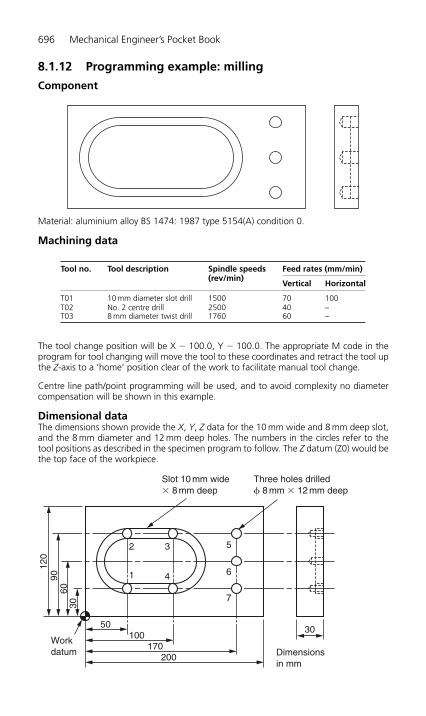
696 Mechanical Engineer’s Pocket Book
Material: aluminium alloy BS 1474: 1987 type 5154(A) condition 0.
Machining data
Tool no. Tool description Spindle speeds Feed rates (mm/min)(rev/min)
Vertical Horizontal
T01 10 mm diameter slot drill 1500 70 100T02 No. 2 centre drill 2500 40 –T03 8 mm diameter twist drill 1760 60 –
The tool change position will be X � 100.0, Y � 100.0. The appropriate M code in theprogram for tool changing will move the tool to these coordinates and retract the tool upthe Z-axis to a ‘home’ position clear of the work to facilitate manual tool change.
Centre line path/point programming will be used, and to avoid complexity no diametercompensation will be shown in this example.
Dimensional dataThe dimensions shown provide the X, Y, Z data for the 10 mm wide and 8 mm deep slot,and the 8 mm diameter and 12 mm deep holes. The numbers in the circles refer to thetool positions as described in the specimen program to follow. The Z datum (Z0) would bethe top face of the workpiece.
Dimensionsin mm
200170
10050 30
7
6
532
1 4
3060
9012
0
Workdatum
Slot 10 mm wide� 8 mm deep
Three holes drilled� 8 mm � 12 mm deep
8.1.12 Programming example: milling
Component
H6508-Ch08.qxd 9/12/05 4:52 PM Page 696

Specimen programThe format of the following program example would be suitable for the Bridgeport BOSS6 software. When evaluating the program, reference should be made to the coded infor-mation given in Section 8.1.7.
CNC listing Description
% Per cent symbol � start of program/tape.
N5 G90 G71 G00 G75 Set up default preparatory codes. G75 is special to BOSS 6 software.
N10 X � 100.0 Y � 100.0 S1500 Rapid move to tool change (home) position. Set spindle speed T01 M06 (rev/min). Select tool required and insert first tool (slot drill). Stop
control for tool change.
N15 X50.0 Y30.0 Restart control. Rapid move to position 1.
N20 Z1.0 M03 Rapid tool move to 1.0 mm above workpiece. Start up spindle (speed set in block N10).
N25 G01 Z � 8.0 F70 M07 Linear feed rate move to required depth (70 mm/min). Mist coolant on.
N30 G02 X50.0 Y90.0 150.0 Circular interpolation to X and Y coordinates at position 2, using J60.0 F100 I and J coordinates for interpolation centers. Increase feed rate
(horizontal) to 100 mm/min.
N35 G01 X100.0 Y90.0 Linear feed rate move as set in block N30 to position 3.
N40 G02 X100.0 Y30.0 Circular interpolation to X and Y coordinates at position 4 at feed 100.0 J60.0 rate set in block N30.
N45 G01 X50.0 Y30.0 Linear feed rate move as set in block N30 to position 1.
N50 G00 Z1.0 Rapid move tool clear of workpiece along Z-axis.
N55 X � 100.0 Y � 100.0 S2500 Rapid move to tool change (home) position and stop spindle. T02 M06 Remove tool 1 and insert tool 2 (center drill). Set spindle speed to
2500 rev/min ready for drilling.
N60 X170.0 Y90.0 Restart control. Rapid move to position 5.
N65 Z1.0 M03 Rapid move to 1.0 mm above workpiece. Start up spindle (speed set to 2500 rev/min in block N55).
N70 G81 X170.0 Y90.0 Z � 5.0 Start drilling cycle (see Section 8.1.11) and centre drill first hole F40 M07 (position 5) to depth at 40 mm/min feed rate. Mist coolant on.
N75 X170.0 Y60.0 C/drill second hole (position 6).
N80 X170.0 Y30.0 C/drill third hole (position 7).
N85 G80 Cancel drilling cycle.
N90 G00 � X100.0 Y � 100.0 Rapid move to tool change (home) position and stop spindle. S1760 T03 M06 Remove tool 2. Insert tool 3 (twist drill). Set spindle speed to
1760 rev/min ready for drilling.
N95 X170.0 Y90.0 Rapid move to position 5.
N100 Z1.0 M03 Rapid move tool to 1 mm above workpiece. Start spindle.
N105 G81 X170.0 Y90.0 Z � Start drilling cycle and drill first hole to depth (12 mm) at position 12.0 F60 M07 5 with 60 mm/min feed rate. Mist coolant on.
N110 X170.0 Y60.0 Drill second hole (position 6).
N115 X170.0 Y30.0 Drill third hole (position 7).
N120 G80 Turn spindle off.
N125 G00 X � 100.0 Y � Return tool to tool change (home) position and stop spindle. 100.0 M06 Ready for repeat of program.
N130 M02 End or program.
N135 M30 End of tape.
Computer-Aided Engineering 697
H6508-Ch08.qxd 9/12/05 4:52 PM Page 697

698 Mechanical Engineer’s Pocket Book
8.1.13 Tool offsets: lathe
On a CNC lathe, to keep a common datum with all the tools on the turret, TLO arerequired in both the X- and Z-axis as shown.
Workpiece
Work datumx0z0
X offset
Z offset
Cutting tool
Turret
Tool change (home)position
Tool no. 1Finish turning tool
Tool no. 4
Tool no. 3
Tool no. 2Screw cuttingtool
U/cutpart-off tool
Roughing turning tool
Direction ofturret rotation
H6508-Ch08.qxd 9/12/05 4:52 PM Page 698

Computer-Aided Engineering 699
On a CNC centre lathe the turret will hold a number of different tools. Each tool will have its own X and Z offset, which will become operative when the tool is called into theprogram. When the turret is indexed all the tools will take up a different position relativeto the workpiece. As can be seen in the diagram, since the various tools protrude fromthe turret by different distances in terms of X and Z, different TLO will need to be set foreach tool.
8.1.14 Tool nose radius compensation: lathe
Tool nose radius compensation (TNRC) is used in a similar manner to diameter compen-sation when milling. Consequently the same preparatory codes (G codes) are used to acti-vate and deactivate TNRC. TNRC reduces the complex and repetitive calculations requiredfor tool paths. The programmer can program as if sharp pointed tools were being used.The codes are as follows:
G41 Compensates tool nose radius to the leftG42 Compensates tool nose radius to the rightG40 Cancels tool nose radius compensation
G41 Compensation to the left
H6508-Ch08.qxd 9/12/05 4:52 PM Page 699
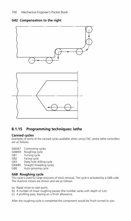
700 Mechanical Engineer’s Pocket Book
G42 Compensation to the right
8.1.15 Programming techniques: lathe
Canned cyclesExamples of some of the canned cycles available when using CNC centre lathe controllersare as follows:
G66/67 Contouring cyclesG68/69 Roughing cycleG81 Turning cycleG82 Facing cycleG83 Deep hole drilling cycleG84/85 Straight threading cyclesG88 Auto grooving cycle
G68 Roughing cycleThis cycle is used for large amounts of stock removal. The cycle is activated by a G68 code.The machine moves are shown and are as follows:
(a) Rapid move to start point.(b) A number of linear roughing passes (the number varies with depth of cut).(c) A profiling pass, leaving on a finish allowance.
After the roughing cycle is completed the component would be finish turned to size.
H6508-Ch08.qxd 9/12/05 4:52 PM Page 700
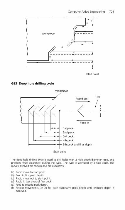
Computer-Aided Engineering 701
G83 Deep hole drilling cycle
Start point
Workpiece
Workpiece
Rapid outDrill
Feed in
1st peck
2nd peck
3rd peck
4th peck
5th peck and final depth
Start point
The deep hole drilling cycle is used to drill holes with a high depth/diameter ratio, andprovides ‘flute clearance’ during the cycle. The cycle is activated by a G83 code. Themoves involved are shown and are as follows:
(a) Rapid move to start point.(b) Feed to first peck depth.(c) Rapid move out to start point.(d) Rapid in just short of first peck.(e) Feed to second peck depth.(f) Repeat movements (c)–(e) for each successive peck depth until required depth is
achieved.
H6508-Ch08.qxd 9/12/05 4:52 PM Page 701

702 Mechanical Engineer’s Pocket Book
8.1.16 Programming example: lathe
An example CNC program follows. The program is to:
(a) Rough turn leaving 0.5 mm on diameters and faces(b) Finish turn the part to size(c) Part off to length.
Component
Work datumX0Z0
Stock
038 036 034 031.5
15
30
45
Dimensions in mm
Material: aluminium alloy BS 1474: 1987 type 5154(A) condition 0.
Tool and machining data
Tool no. Tool description Spindle speed Feed rates (mm/rev)
T101 Turning tool for roughing 130 m/min 0.2T202 Turning tool for finishing 2500 rev/min 0.05T303 Part off tool 120 m/min 0.05
Specimen program(a) The format of the program would be suitable for a GE 1050 CNC controller.(b) Diameter programming is used in this example.(c) Tool change position (home position) is X177.8 Z254.
CNC program listing Description
% Start of program/tape.
N0010 G71 Metric input.
N0020 G95 Feed rate, mm/rev.
N0030 G97 S1000 M03 Direct rev/min spindle speed. 1000 rev/min switch on spindle.
N0040 G00 M08 Rapid move set. Switch on coolant.
N0050 G53 X177.8 Z254.0 T0 Cancels work offset. Moves turret to home position. Cancels tool offsets.
N0060 T100 Rotates turret to position 1.
continued
H6508-Ch08.qxd 9/12/05 4:52 PM Page 702

Table (continued )
CNC program listing Description
N0070 G54 X00 Z2.0 T101 Activates work offset. Rapid move to coordinates. Activates tool offset number 1 with tool number 1.
N0080 G92 R0 S2000 Sets up parameters for constant surface cutting speed (CSS) (maximum 2000 rev/min).
N0090 G96 S130 Activates CSS at 130 m/min.
N0100 G01 X0.0 Z0.5 F0.2 Linear feed rate move at 0.2 mm/rev.
N0110 X36.5 Linear feed rate move at 0.2 mm/rev.
N0120 Z50.0 Turning beyond end of component to reduce diameter for parting off. Linear feed rate moves at 0.2 mm/rev.
N0130 G00 X37.0 Rapid move of tool off workpiece.
N0140 Z0.5 Rapid move of tool off workpiece.
N0150 X34.5 Rapid move of tool off workpiece.
N0160 G01 Z � 29.5 Linear feed rate move.
N170 G00 X35.0 Rapid move.
N0180 Z0.5 Rapid move.
N0190 X32.0 Rapid move.
N0200 G01 Z � 14.5 Linear feed rate move.
N0120 G00 Rapid move.
N0220 G53 X177.8 Z254.0 T0 Cancels work and tool offsets and moves turret to home position.
N0230 T200 Rotates turret to position 2.
N0240 G54 X10.0 Z10.0 T202 Activates work offset. Rapid move to coordinates. Activates tool offset number 2 with tool number 2.
N0250 G41 X0.0 Z0.05 Moves to coordinates and activates TNRC.
N0260 G97 S2500 Direct rev/min, 2500 rev/min.
N0270 G01 Z0.0 F0.05 Linear feed rate move at 0.05 mm/rev.
N0280 X31.5 Linear feed rate moves to profile part to size.
N0290 Z � 15.0
N0300 X34.0
N0310 Z � 30.0
N0320 X36.0
N0330 Z � 45.0
N0340 G40 Cancels TNRC.
N0350 G00 Rapid move.
N0360 G53 X177.8 Z254.0 T0 Cancels work offset. Rapid move to home position. Cancelstool offsets.
N0370 T300 Rotates turret to position 3.
N0380 G54 X38.0 Z � 45 T303 Activates work offset. Rapid move to coordinates. Activates tool offset number 3 with tool number 3.
N0390 G92 R38 S1000 Sets up parameters for CSS.
N0400 G96 S120 Activates CSS at 120 m/min.
N0410 G01 X � 2.0 F0.05 Linear feed rate move.
N0420 G00 X38.0 M05 Rapid clear of work. Switch off spindle.
N0430 G53 X177.8 Z254.0 T0 Cancels work and tool offsets. Rapid to home position.
N0440 M02 End of program.
Computer-Aided Engineering 703
H6508-Ch08.qxd 9/12/05 4:52 PM Page 703

704 Mechanical Engineer’s Pocket Book
8.1.17 Glossary of terms
Absolute programming A system of programming where all positional dimensionsare related to a common datum.
Adaptive control A system of sensors which changes speeds/feeds in response tochanges in cutting loads. Also provides for in-process gauging and size correction.
Address In programming, a symbol which indicates the significance of the informationimmediately following that symbol.
Backlash ‘Wasted’ movements between interacting mechanical parts due to wearand/or manufacturing tolerance.
Binary coded decimal A method of representing decimal numbers by a series ofbinary numbers.
Binary number A number system with a base of 2.
Bit An abbreviation of ‘binary digit’.
Block A line or group of words which contains all the instructions for one operation.
Byte A group of 8 bits.
CAM Computer-aided manufacture.
Canned cycle An operation which has been preprogrammed and which can be calledup by a single instruction.
Circular interpolation A type of contouring control which uses the information con-tained in a single instruction to produce movement along the arc of a circle.
CLF Cutter location file.
Closed-loop control A system in which a signal depending on the output is fed backto a comparing device so that the output can be compared with the input, and a correct-ive signal generated if necessary.
Continuous path system A system in which the tool path results from the coord-inated simultaneous motion of the work and/or cutter along two or more axes.
Cutter compensation An adjustment which compensates for the difference betweenthe actual and programmed cutter diameters. See also Tool length offset (TLO).
Datum The reference position from which all absolute coordinates are taken.
DNC Direct numerical control.
DO loop A loop back to a repeated instruction in a program.
Encoder A device which is used to convert the position of a moving device into an elec-tronic signal.
H6508-Ch08.qxd 9/12/05 4:52 PM Page 704

Feed rate The rate at which the cutting tool is advanced into the workpiece.
Incremental system A system by which each positional dimension is measured fromthe preceding position.
In-process gauging A system of gauging built into the machine which gauges thework whilst it is being manufacture so that any errors due to tool wear can be compen-sated for automatically. In the event of tool failure the machine will automatically change to back-up tooling. Thus the machine can be used unattended in a ‘lightsout’environment. Used in conjunction with adaptive control.
Interpolation The joining up of programmed points to make a smooth curve by computation.
Linear path system A point-to-point system in which the tool or work moves only instraight lines.
Manual data input (MDI) A means of manually entering instructions to a controller,usually via a key panel.
Numerical control Control of machine movements by the direct insertion of numeri-cal data.
Open-loop system A system where there is a single forward path between the inputinstruction and the output signal with no feedback.
Parallel path system A point-to-point system in which the tool or work moves only instraight lines parallel to any axis.
Parity A checking method to help determine if the tape has been prepared correctly.The standard for even parity is that of the International Standards Organization (ISO),whereas the standard for odd parity is that of the Electronic Industries Association (EIA).
Part program A program in machine control language and format required to accom-plish a given task.
Point-to-point system A system in which the controlled motion is required only toreach a given end point, with no path control during the movements from one point tothe next.
Post-processor A set of computer instructions which transforms tool centre line datainto machine movement commands using the tape code and format required by a spe-cific machine tool control system.
Rapid traverse Movements at a high traverse rate, normally used to save time whenpositioning the cutter before cutting commences.
Servo system An automatic control system, incorporating power amplification andfeedback, designed to make a machine table follow the programmed route.
Spindle speed The rotational speed of the cutting tool or workpiece.
Subroutine A sequence of instructions or statements used to perform an operationwhich is frequently required. It is prepared by the part programmer and temporarily storedin the controller memory.
Computer-Aided Engineering 705
H6508-Ch08.qxd 9/12/05 4:52 PM Page 705

706 Mechanical Engineer’s Pocket Book
Tape punch A device for transferring instructions to a punched tape by perforating itwith holes.
Tape reader A device for sensing and transmitting the instructions recorded on apunched or magnetic tape.
Tool length offset (TLO) An instruction which adjusts the position of the spindlealong the Z-axis of a milling machine to take account of different lengths of cutting tool.On a lathe, offset is parallel to both the X- and Z-axis.
Word A set of characters which give a single complete instruction to a machine’s con-trol system.
Word address A block of characters preceded by a literal symbol to identify them.
8.2 Computer-aided design
8.2.1 An introduction to computer-aided design
Computer-aided design (CAD) is the application of a computer system which can be usedto solve or enhance the solution of design and draughting problems. It not only eases thework of the draughtsperson in preparing drawings in both 2D and 3D, but it can beextended to provide:
● Geometric modelling: wire frame and solid modelling.● Finite element analysis techniques to solve thermal and mechanical stress problems.● Testing.● Documentation.● CNC programming.
For the architect and civil engineer, the ability to draw not only individual buildings butwhole estates and complexes in 3D and then change the viewpoint at the touch of a but-ton is of inestimable value. The use of virtual reality techniques enables the designer to‘walk through’ an estate or complex.
By far the most widely used application of CAD in small- and medium-engineering com-panies is as a draughting aid. The capabilities of a typical draughting system could be:
● The production of ‘library symbols’ such as BS 308 conventions, pneumatic symbols,hydraulic symbols, electrical symbols and electronic symbols.
● The production of three view orthographical drawings using these symbols, to avoidhaving to repeatedly draw small details (e.g. screwed fastenings).
● The automatic production of isometric an oblique drawings from orthographical draw-ings and the ability to change the viewpoint at will.
● Drawing can be speeded up by such commands as: mirror imaging, rotation, copying,move, zoom, scaling, fillets, rectangles and polygons.
● The automatic shading or hatching of section drawings.● The facility to make major or minor changes to a drawing without redrawing.● The production of printed circuit board (PCB) layouts.● The production of plant layouts.● The production of parts lists, bills of materials, etc., directly from the digitized drawing data.● Ease of storage on floppy disks.
Some typical examples of drawings are shown below. These were produced on DesignCADand are reproduced by courtesy of P.M.S (Instruments) Ltd.
H6508-Ch08.qxd 9/12/05 4:52 PM Page 706
Computer-Aided Engineering 707
H6508-Ch08.qxd 9/12/05 4:52 PM Page 707
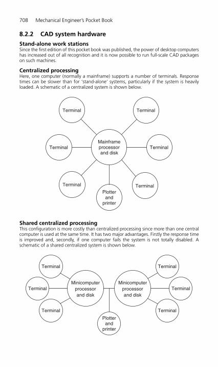
708 Mechanical Engineer’s Pocket Book
8.2.2 CAD system hardware
Stand-alone work stationsSince the first edition of this pocket book was published, the power of desktop computershas increased out of all recognition and it is now possible to run full-scale CAD packageson such machines.
Centralized processingHere, one computer (normally a mainframe) supports a number of terminals. Responsetimes can be slower than for ‘stand-alone’ systems, particularly if the system is heavilyloaded. A schematic of a centralized system is shown below.
Terminal Terminal
Terminal
Terminal Terminal
Terminal
Plotterand
printer
Mainframeprocessorand disk
Shared centralized processingThis configuration is more costly than centralized processing since more than one centralcomputer is used at the same time. It has two major advantages. Firstly the response timeis improved and, secondly, if one computer fails the system is not totally disabled. Aschematic of a shared centralized system is shown below.
Plotterand
printer
Terminal
TerminalTerminal
Minicomputerprocessorand disk
Minicomputerprocessorand disk
TerminalTerminal
Terminal
H6508-Ch08.qxd 9/12/05 4:52 PM Page 708
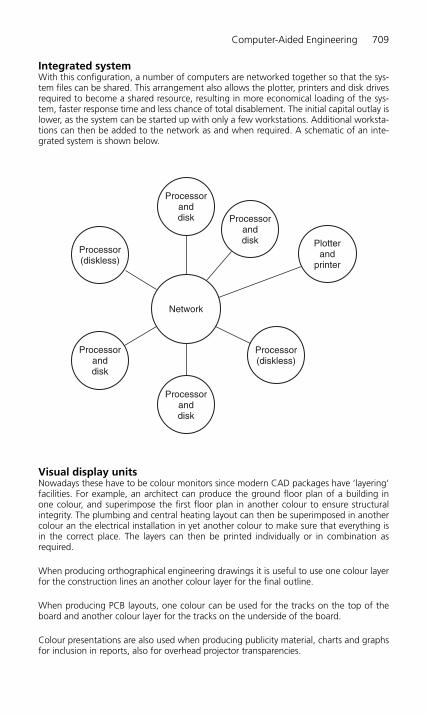
Computer-Aided Engineering 709
Integrated systemWith this configuration, a number of computers are networked together so that the sys-tem files can be shared. This arrangement also allows the plotter, printers and disk drivesrequired to become a shared resource, resulting in more economical loading of the sys-tem, faster response time and less chance of total disablement. The initial capital outlay islower, as the system can be started up with only a few workstations. Additional worksta-tions can then be added to the network as and when required. A schematic of an inte-grated system is shown below.
Network
Processor(diskless)
Processor(diskless)
Processoranddisk
Processoranddisk
Processoranddisk Processor
anddisk Plotter
andprinter
Visual display unitsNowadays these have to be colour monitors since modern CAD packages have ‘layering’facilities. For example, an architect can produce the ground floor plan of a building in one colour, and superimpose the first floor plan in another colour to ensure structuralintegrity. The plumbing and central heating layout can then be superimposed in anothercolour an the electrical installation in yet another colour to make sure that everything is in the correct place. The layers can then be printed individually or in combination asrequired.
When producing orthographical engineering drawings it is useful to use one colour layerfor the construction lines an another colour layer for the final outline.
When producing PCB layouts, one colour can be used for the tracks on the top of theboard and another colour layer for the tracks on the underside of the board.
Colour presentations are also used when producing publicity material, charts and graphsfor inclusion in reports, also for overhead projector transparencies.
H6508-Ch08.qxd 9/12/05 4:52 PM Page 709

710 Mechanical Engineer’s Pocket Book
Input devicesKeyboards These are familiar to all computer operators and are user friendly. These areused to input commands, text and parameter values.
Digitizer tablet The data tablet detects the position of a mechanical scanning or hand-held cursor. The tablet contains an electromagnetic, electrostatic or electroresistive gridwhich corresponds to the resolution of the visual display unit (VDU). Thus, X and Y coord-inates on the tablet can be mapped directly on to the screen.
Joystick This is a two-axes control for providing a rapid movement of the cursor. It isfamiliar to players of video games. When used with CAD systems it allows more rapid cur-sor movement than is possible from the keyboard. However, the positional accuracy is lowand is dependent on operator skill.
Mouse The mouse is now widely used in place of the joystick and is essential whenusing Windows versions of CAD software. The ‘click’ keys on the mouse allow the com-mand to be entered quickly and easily once the cursor has been positioned.
Output devicesHard copy can be printed from digitized data in a number of ways.
Flat bed plotter The paper is held to the flat bed of the machine by suction. The penmoves along the X- and Y-axis to draw the image. The carriage moves along the X-axisand the penhead moves along the Y-axis bridge which is located on the carriage. There isalso a ‘home’ position to which the penhead is parked at the start and finish of the draw-ing. This allows the paper to be inserted and the finished drawing removed without foul-ing the pen. The penhead also returns to the ‘home’ position when the pen has to bechanged to accommodate a different line thickness and/or colour. The pens are located ina magazine and are selected on command from the computer.
Drum or roller bed plotter The bed rotates to provide the X-axis movement and thepen carriage moves along the Y-axis parallel to the drum axis of rotation. This arrange-ment allows large drawings to be produced, yet little floor space is required. These plot-ters are not quite so accurate as flat bed plotters due to paper stretch and slip. They arealso more limited in the range of materials that they will accept.
For small-scale drawings, conventional dot matrix, laser jet and electrostatic printers asused for normal text hard copy printing are suitable.
8.2.3 CAD system software
There are now many CAD packages available. These may be in 2D or 3D. Generally, a 2Dpackage will do anything that can be done manually using a drawing board and T-squaretogether with conventional drawing instruments. You can also produce isometric andoblique ‘pictorial’ representations. To save time it is possible to purchase ‘libraries’ of stand-ard symbols. Some companies provide library information of their products on disk fortheir customers to use. For example, manufacturers of bathroom and kitchen fittings pro-vide scale drawings of their product range on disk for architects to import directly intotheir designs. Some users will build up their own libraries of frequently used componentsusing ‘block’ commands.
3D software is necessary when you require:
● Wire frame modelling This described the corners and edges of a model as shownbelow. It can lead to a view looking ambiguous.
H6508-Ch08.qxd 9/12/05 4:52 PM Page 710

Computer-Aided Engineering 711
● Surface models These are usually used when components have a complex surface,such as a car or an aircraft panel. Information relating to the surface can be extractedfrom the shaded surface model.
● Solid models These provide detailed information concerning areas, volumes andcentre of gravity of a component part. Solid models can be built up from standard 3Dshapes and modified to get the desired result.
All CAD software in current use is configured to run in a Windows environment but someversions are available for use with Mackintosh computers. There is a wide range of soft-ware packages available configured for use by engineering designers, architects, interiordesigners, nautical architects and others. They invariably have provision for customisingby the user to suit specific applications and are supported by ‘libraries’ of data and sym-bols that can be selected as required. Although requiring massive computer power com-pared with earlier versions, the latest, modern desk-top and lap-top computers can stillsupport most of the packages in common use.
8.2.4 Computer-aided design and manufacture
The integration of CAD with computer-aided manufacture (CAM) involves the sharing ofa database between these distinct elements. The advantages of such a system are:
● There is consistent reliability of information relating to design and manufacture with-out the possibility of copying errors.
● CNC programmes can be constructed directly from the digitized data of the drawingin much shorter times.
● Complex parts are programmed without the need for lengthy calculations.
H6508-Ch08.qxd 9/12/05 4:52 PM Page 711

● On-screen proofing of CNC program tool paths reduces the possibility of scrappedcomponents and damaged cutting tools.
● The reduction of lead time between the design stage and the completion of manufacture.
8.2.5 Advantages and limitations of CAD
Advantages● There are substantial improvements in productivity during the design and draughting
process.● Drawings can be produced to very high levels of accuracy and consistent house styles.● Product design can be improved.● It is easy to make modifications without completely redrawing.● The storing of digitized data on disk is simple and storage space is reduced compared
with tracings.● Colour coded hard copy can be produced whereas conventional dyeline prints are
monochrome.● Digitized data can be used for: costing and estimating, purchasing, production plan-
ning and control, control of labour costs, quality control.● Digitized CAD data can be integrated with CNC machines (CAD/CAM) and also with
robots to provide flexible manufacturing systems (FMS).
Limitations● Hardware and software costs for CAD can be very high. Although the cost of individual
components may be reduced, the continual increase in the complexity and sophistica-tion of the software demands greater and greater memory capacity and greater powerand speed from the CPU. This overtakes any cost reductions in individual components.
● Powerful CAD systems require regular maintenance, although they are becoming verymuch more reliable and maintenance contracts are available.
● Initial set-up and staff training can be expensive whilst libraries of conventions an sym-bols are prepared and digitized to suit company products.
● A suitable ergonomic environment is required to avoid operator fatigue and ensureeconomic use of the system.
8.3 Industrial robots
8.3.1 An introduction to robotics
An industrial robot is a general purpose, programmable machine possessing certainanthropomorphic (human-like) characteristics. The most typical anthropomorphic charac-teristic of a robot is its arm. This arm, together with the robot’s capability to be pro-grammed, makes it ideally suited to a variety of production tasks, including machineloading, spot welding, spray painting and assembly. The robot can be programmed to per-form a sequence of mechanical motions, and it can repeat that motion sequence indefin-itely until reprogrammed to perform some other job.
Manufacturers use robots mostly to reduce manning levels. Robots, used either withother robots or with other machines, have two major advantages compared with trad-itional machines. First, they allow almost total automation of production processes, lead-ing to increased rates of production better quality control and an increased response tovarying demand. Second, they permit the adaptability, at speed, of the production unit.The production line can be switched rapidly from one product to another similar product,for example from one model of car to another. Again, when a breakdown immobilizesone element in the production unit, that element’s function can be replaced quickly.
712 Mechanical Engineer’s Pocket Book
H6508-Ch08.qxd 9/12/05 4:52 PM Page 712

Computer-Aided Engineering 713
Adaptable production units are known as FMS. A flexible unit would comprise a small num-ber of robots and computer-controlled machine tools working together to produce or part-produce a particular component or assembly. The logical development of such systems is tointegrate a number of these flexible cells into a fully automated workshop or factory.
It must be remembered that the robot, although a highly sophisticated device, cannot byitself solve all the problems that can be solved by the human operator. It must thereforebe associated with additional techniques (e.g. CAM).
The term robotics has two currently accepted meanings:
(a) In the strictest sense of the word, it implies the further development of automation byimproving the robot as we know it at present.
(b) In the broader sense, it involves the development not only of the robot itself, but alsoprocesses associated with the robot (e.g. CAD) or the consideration of the robot as amachine with special properties in association with other machines (e.g. flexible manu-facturing cells or systems).
8.3.2 Robot control
An industrial robot shares many attributes in common with a CNC machine tool. The type of technology used to operate CNC machine tools is also used to actuate the robot’smechanical arm. However, the uses of the robot are more general, typically involving thehandling of work parts. Robots can be programmed from a computer on-line or off-line.Alternatively, the robot can be guided through a sequence of movements from a remotekey pad coupled to the robot by a trailing lead. Thirdly, the robot can be guided manuallythrough a sequence of movements as when spray painting, with the human operatorholding and directing the robot’s spray gun. The instructions are retained in the robot’selectronic memory. In spite of these differences, there are definite similarities betweenrobots and CNC machine tools in terms of power drive technologies, feedback systems,the use of computer control and even some of the industrial applications.
8.3.3 Robot arm geometry
A robot must be able to reach workpieces and tools. This requires a combination of anarm and a wrist subassembly, plus a ‘hand’, usually called the end effector. The robot’ssphere of influence is based on the volume into which the robot’s arm can deliver thewrist subassembly. A variety of geometric configurations have been researched and theirrelative kinematic capabilities appraised. To date, the robot manufacturers have special-ized in the following geometric configurations:
(a) Cartesian coordinates: three linear axes.(b) Cylindrical coordinates: two linear axes and one rotary axis.(c) Spherical coordinates: one linear axis and two rotary axes.(d) Revolute coordinates: three rotary axes.
Cartesian coordinate robotsCartesian coordinate robots consist of three orthogonal linear sliding axes, the manipula-tor hardware and the interpolator. The control algorithms are similar to those of CNCmachine tools. Therefore, the arm resolution and accuracy will also be of the order ofmagnitude of machine tool resolution.
An important feature of a cartesian robot is its equal and constant spatial resolution; thatis, the resolution is fixed in all axes of motions and throughout the work volume of therobot arm. This is not the case with other coordinate systems.
H6508-Ch08.qxd 9/12/05 4:52 PM Page 713
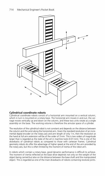
714 Mechanical Engineer’s Pocket Book
Cylindrical coordinate robotsCylindrical coordinate robots consist of a horizontal arm mounted on a vertical column,which in turn is mounted on a rotary base. The horizontal arm moves in and out, the car-riage moves vertically up and down on the column, and these two units rotate as a singleassembly on the base. The working volume is therefore the annular space of a cylinder.
The resolution of the cylindrical robot is not constant and depends on the distance betweenthe column and the wrist along the horizontal arm. Given the standard resolution of an incre-mental digital encoder on the rotary axis and arm length of only 1 m, then the resolution atthe hand at full arm extension will be of the order of 3 mm. This is two orders of magnitudelarger than is regarded as the state of the art in machine tools (0.01 mm). This is one of thedrawbacks of cylindrical robots as compared to those with cartesian frames. Cylindricalgeometry robots do offer the advantage of higher speed at the end of the arm provided bythe rotary axis, but this is often limited by the moment of inertia of the robot arm.
In robots which contain a rotary base, good dynamic performance is difficult to achieve.The moment of inertia reflected at the base drive depends not only on the weight of theobject being carried but also on the distance between the base shaft and the manipulatedobject. This is regarded as one of the main drawbacks of robots containing revolute joints.
ZY
X
H6508-Ch08.qxd 9/12/05 4:52 PM Page 714
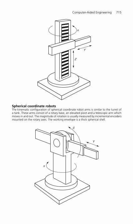
Computer-Aided Engineering 715
Z
Y
u
Spherical coordinate robotsThe kinematic configuration of spherical coordinate robot arms is similar to the turret ofa tank. These arms consist of a rotary base, an elevated pivot and a telescopic arm whichmoves in and out. The magnitude of rotation is usually measured by incremental encodersmounted on the rotary axes. The working envelope is a thick spherical shell.
Y
b
u
H6508-Ch08.qxd 9/12/05 4:52 PM Page 715
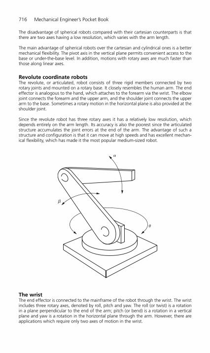
716 Mechanical Engineer’s Pocket Book
The disadvantage of spherical robots compared with their cartesian counterparts is thatthere are two axes having a low resolution, which varies with the arm length.
The main advantage of spherical robots over the cartesian and cylindrical ones is a bettermechanical flexibility. The pivot axis in the vertical plane permits convenient access to thebase or under-the-base level. In addition, motions with rotary axes are much faster thanthose along linear axes.
Revolute coordinate robotsThe revolute, or articulated, robot consists of three rigid members connected by tworotary joints and mounted on a rotary base. It closely resembles the human arm. The endeffector is analogous to the hand, which attaches to the forearm via the wrist. The elbowjoint connects the forearm and the upper arm, and the shoulder joint connects the upperarm to the base. Sometimes a rotary motion in the horizontal plane is also provided at theshoulder joint.
Since the revolute robot has three rotary axes it has a relatively low resolution, whichdepends entirely on the arm length. Its accuracy is also the poorest since the articulatedstructure accumulates the joint errors at the end of the arm. The advantage of such astructure and configuration is that it can move at high speeds and has excellent mechan-ical flexibility, which has made it the most popular medium-sized robot.
a
b
u
The wristThe end effector is connected to the mainframe of the robot through the wrist. The wristincludes three rotary axes, denoted by roll, pitch and yaw. The roll (or twist) is a rotationin a plane perpendicular to the end of the arm; pitch (or bend) is a rotation in a verticalplane and yaw is a rotation in the horizontal plane through the arm. However, there areapplications which require only two axes of motion in the wrist.
H6508-Ch08.qxd 9/12/05 4:52 PM Page 716
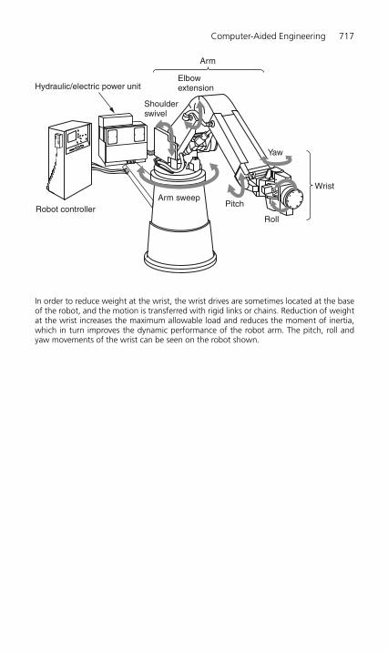
Computer-Aided Engineering 717
In order to reduce weight at the wrist, the wrist drives are sometimes located at the baseof the robot, and the motion is transferred with rigid links or chains. Reduction of weightat the wrist increases the maximum allowable load and reduces the moment of inertia,which in turn improves the dynamic performance of the robot arm. The pitch, roll andyaw movements of the wrist can be seen on the robot shown.
Robot controllerArm sweep
Pitch
Roll
Wrist
Yaw
Arm
Elbowextension
Shoulderswivel
Hydraulic/electric power unit
H6508-Ch08.qxd 9/12/05 4:52 PM Page 717

Appendix 1
BSI Standards: Sales Order and Enquiry Contacts
BSI standards provides a variety of products and services to help standards users to man-age their collection and to make standards work for their organization. The following is abrief summary of the services available and appropriate contact numbers.
Customer services
Tel.: 0181 996 7000Fax: 0181 996 7001
– for identifying, price quotations andordering British and Foreign standardsand other publications
– “PLUS” – private list updating service
Information centre
Tel.: 0181 996 7111Fax: 0181 996 7048
– for detailed information and searcheson British and overseas standards
– technical help to exporters– certification and testing requirements
overseas– EC standardization developments
Membership services
Tel.: 0181 996 7002Fax: 0181 996 7001
– members help desk– membership administration
Translations and languageservices
Tel.: 0181 996 7222Fax: 0181 996 7047
– for technical, standards and commercialtranslations
Copyright
Tel.: 0181 996 7070Fax: 0181 996 7400
– copyright licences and enquiries
Library services
Tel.: 0181 996 7004Fax: 0181 996 7005
– library services and enquiries
Electronic products helpdesk
Tel.: 0181 996 7333Fax: 0181 996 7047
– perinorm– electronic product development
H6508-App1.qxd 9/12/05 4:36 PM Page 718

Appendix 1: BSI Standards 719
Ordering BSI publications
Orders can be placed by post, phone, faxor telex through BSI customer services.Post: BSI customer services
BSI Standards389 Chiswick High RoadLondon W4 4AL
Tel.: 0181 996 7000Fax: 0181 996 7001
The hours of opening are 8.30 am to 5.30 pm Mondays to Fridays except publicholidays
PLUSPrivate list updating service
Contact: Tel.: 0181 996 7398Fax: 0181 996 7001
Electronic media and databases – Helpdesk
Contact: Fax: 0181 996 7047
Copyright licencesContact: Pamela Danvers
Tel.: 0181 996 7070Fax: 0181 996 7001
Non-members
Non-members should send remittance withorder, based on the prices given, or paydirectly by credit card.
Members
Members will be invoiced in the usual wayand will receive the appropriate discounts.
Prices
The group (Gr) number of each entry, inconjunction with the key below, indicates
the UK price of the document. Postageand packing is included
Group Non- Membersno. members
0 2.60 1.301 2.60 1.302 6.70 3.353 12.00 6.004 17.50 8.755 26.00 13.006 32.60 16.307 47.00 23.508 61.50 30.759 72.50 36.25
10 86.50 43.2511 92.00 46.0012 104.00 52.0013 116.50 58.2514 127.50 63.7515 130.00 65.00
The above prices are for guidance and may besubject to variation.
Members’ order hotline
Tel.: 0181 996 7003
For members who know exactly what theywant to order.
Speeds up the placing of telephone orders.
Priority service
Urgent orders received before 12.00 h, byphone, fax or telex can be sent by priorityservice and will be despatched on thesame day by first class mail (orders for thepriority service should be clearly marked ).
The charge for this service is 10% ofinvoice value, with a minimum charge of£1.00 and a maximum charge of £50.00.
Sales outlets
See the BSI catalogue for a full list of BSIsales outlets
H6508-App1.qxd 9/12/05 4:36 PM Page 719

720 Mechanical Engineer’s Pocket Book
Information centre
For detailed information and searches onBritish and overseas standards;
– certification and testing requirementsoverseas;
– technical help to exporters;– EC development re. standardization
Tel.: 0181 996 7021Electrical
Tel.: 0181 996 7022Consumer products
Tel.: 0181 996 7023Construction
Tel.: 0181 996 7024Mechanical
Fax: 0181 996 7048
– Library loans International and foreignstandards and related technical docu-ments are available for loan to BSI mem-bers. The current price of tokens is£35.00 per book for orders or 10 ormore books (please quote token num-bers when requesting items for loan).Library contact:
Tel.: 0181 996 7004Fax: 0181 996 7005
BSi News Updatecompiled and edited by
Kay WestlakeTel.: 0181 996 7060Fax: 0181 996 7089
Membership services
Tel.: 0181 996 7002Fax: 0181 996 7001
Translations and language services
Tel: 0181 996 7222Fax: 0181 996 7047
– for technical, standards and commercialtranslations
Copyright
Copyright subsists in all BSI publications. BSI also holds the copyright, in the UK,of the publications of the international standardization bodies. Except as permittedunder the Copyright, Design and PatentsAct 1988 no extract may be reproduced,stored in a retrieval system or transmitted inany form or by any means – electronic, pho-tocopying, recording or otherwise – withoutprior written permission from BSI. If permis-sion is granted, the terms may include roy-alty payments or a licensing agreement.
Details and advice can be obtained from the:
Copyright Manager,BSI, 389 Chiswick High Road,London W4 4AL
Tel.: 0181 996 7070
BSI print on demand policy
● BSI has revised its production processesfollowing intensive investment andprocess redesign enabling the rapid pro-duction of products on a variety of mediafrom paper to electronic books.
● Increasingly, all British, European andInternational standards you order will beprinted on demand from images storedin electronic files.
● By providing standards as looseleaf, hole-punched documents, amendments canbe integrated more easily as replacementpages to provide improved, up-to-dateand complete working documentation.Eventually the messy and time-consumingcut-and-paste methods will no longer benecessary to update your standards.
● During the transition phase from exist-ing processes the product may arrive invarious formats. We apologize for thisand also for the quality of original mate-rial we have to use until the changeoveris complete. We hope to start receivinglive files from our international col-leagues over the next 12 months whichwill significantly improve the print qual-ity of BS, ISOs and BS EN ISOs.
H6508-App1.qxd 9/12/05 4:36 PM Page 720

Appendix 1: BSI Standards 721
● All of the new-format standards areprinted on special watermarked paperwith the words ‘licenced copy’ inside thepaper, so that you can show that youown the official standard supplied by BSI.
BSI standards
389 Chiswick High RoadLondon W4 4AL
Tel.: 0181 996 9000Fax: 0181 996 7400
Customer services
Tel.: 0181 996 7000Fax: 0181 996 7001
Membership administration
Tel.: 0181 996 7002Fax: 0181 996 7001
Information centre
Tel.: 0181 996 7111Fax: 0181 996 7048
BSI quality assurance
Tel.: 01908 220908Fax: 01908 220671
BSI testing
Tel.: 01442 230442Fax: 01442 321442
BSI product certification
Tel.: 01908 312636Fax: 01908 695157
BSI training services
Tel.: 0181 996 7055Fax: 0181 996 7364
– Materials and chemicals– Health and environment– Consumer products– Engineering– Electrotechnical– Management systems– Information technology– Building and civil engineering
● British standards● Corresponding international standards● European standards● Handbooks and other publications
BSI global
Web site: www.bsi.global.comE-mail: [email protected]
H6508-App1.qxd 9/12/05 4:36 PM Page 721

Appendix 2
Library Sets of British Standards in the UK
The following libraries hold full sets of British standards in either paper, CD-ROM or micro-fiche formats. The names of public libraries are shown in italics. For other libraries, it is advis-able to make prior written application in order to ascertain the hours and conditions foraccess. These sets are for reference only and attention is drawn to Copyright Law.
ENGLANDAvonBath Central Library
University of BathBristol Commercial Library
BedfordshireBedford Central LibraryCranfield Cranfield UniversityLeighton Buzzard Public LibraryLuton Central Library
University of Luton
BerkshireReading Central Library
University of ReadingReading College
Slough Central Library
BuckinghamshireAylesbury County HallHigh Wycombe College of H & EMilton Keynes Central Library
CambridgeshireCambridge Central LibraryPeterborough Central Library
CheshireCrewe Central LibrarySouth Wirral Ellesmere Port
LibraryStockport Central LibraryWarrington Central Library
ClevelandCleveland County Library
Hartlepool Reference LibraryMiddlesbrough University of Teesside
CornwallRedruth Cornwall College of
Further & HigherEducation
Truro Reference Library
CumbriaBarrow-in-Furness County LibraryCarlisle County LibraryKendal County Library
DerbyshireChesterfield Central LibraryDerby University of Derby
DevonBarnstaple Central LibraryExeter Central LibraryPlymouth Reference Library
DorsetPoole Reference Library,
The Dolphin Centre
DurhamDarlington College of
TechnologyDurham County Library
University LibraryNew College
EssexBarking Central Library
H6508-App2.qxd 9/12/05 4:37 PM Page 722

Appendix 2: Library Sets of British Standards in the UK 723
Chelmsford Central LibraryAnglia PolytechnicUniversity
Colchester LibraryIlford Central LibraryRomford Central LibrarySouthend-on-Sea College of Arts &
TechnologySouthend Library
GloucestershireCheltenham County Library
HampshireBasingstoke Public LibraryFarnborough Public LibraryPortsmouth Central Library
Highbury College ofTechnologyUniversity Library ofPortsmouth
Southampton Central LibraryWinchester County Library
Hereford & WorcesterRedditch Redditch Library
HertfordshireHatfield Central Library
University ofHertfordshire
Stevenage Central LibraryWatford Central Library
HumbersideGrimsby Central LibraryHull Central LibraryScunthorpe Central Library
JerseySt Helier The Jersey Library
KentBexley Heath Central LibraryBromely Central LibraryChatham Central LibraryMaidstone County LibraryMargate Public LibraryTonbridge Central Library
LancashireBlackburn Central LibraryBolton Central Library
Institute of HigherEducation
Preston Central LibraryLancashirePolytechnic
LeicestershireLeicester De Montfort
UniversityInformation CentreUniversity ofLeicester
Loughborough University ofTechnology
LincolnshireLincoln Central Library
Greater LondonBattersea Reference LibraryChiswick BSI LibraryCity University Reference LibraryGower Street University College
LondonHammersmith Central LibraryHaringey Middx University,
Bounds GreenCentral Library
Hendon The BurroughsHolborn The British LibraryIslington Central LibraryKensington Imperial College of
ScienceEducational Libraries
Kingston Kingston UniversityPalmers Green Reference LibrarySouthwark South Bank UniversityStratford Newham
Community CollegeReference Library
Swiss Cottage Reference LibraryWaltham Forest Waltham CollegeWestminster University of
WestminsterWestminster Libraries
Woolwich Woolwich CentralLibrary
Greater ManchesterAshton-under-Lyne Public LibraryManchester John Rylands
University LibraryMetro UniversityLibraryPublic LibraryUMIST LibraryUniversity ofManchester
Oldham Reference LibrarySalford College of
TechnologyUniversity of Salford
H6508-App2.qxd 9/12/05 4:37 PM Page 723

724 Mechanical Engineer’s Pocket Book
Wigan Wigan & LeighCollege
MerseysideBirkenhead Central LibraryLiverpool Central Reference
LibraryJohn MooresUniversityUniversity, HaroldCohen Library
St Helens Gamble Institute
MiddlesexUxbridge Brunel University
W MidlandsBirmingham Aston University
Chamberlain SquareUniversity ofBirminghamUniversity of CentralEngland
Coventry Central LibraryCoventry UniversityLanchesterUniversity LibraryUniversity ofWarwick
Dudley Reference LibrarySolihull Central LibraryWalsall Central LibraryWest Bromwich Central LibraryWolverhampton Central Library
NorfolkNorwich County Hall
NorthamptonshireNorthampton Central Library
NorthumberlandAshington College of Arts &
Technology
NottinghamshireNottingham County Library
Trent UniversityLibraryUniversity ofNottingham
OxfordshireDidcot Rutherford Appleton
LaboratoryOxford Central Library
Oxford BrookesUniversity
ShropshireTelford St Quentin Gate
SomersetBridgewater County Library
StaffordshireHanley Library
SuffolkIpswich County LibraryLowestoft Central Library
SurreyCroydon Central LibraryGuildford College of
TechnologySutton Central LibraryWoking Public Library
E SussexBrighton Reference Library
W SussexBrighton University of
BrightonCrawley Public Library
Tyne and WearGateshead Central LibraryNewcastle Central Library
Polytechnic Universityof Newcastle
North Shields Central LibrarySouth Shields Central Library
South TynesideCollege
Sunderland County LibraryUniversity ofSunderland
Washington Central Library
WarwickshireRugby Central Library
WiltshireTrowbridge Public Library
N YorkshireNorthallerton County LibraryYork Askham Bryan
CollegeCentral Library
S YorkshireBarnsley Central LibraryDoncaster Central Library
H6508-App2.qxd 9/12/05 4:37 PM Page 724

Appendix 2: Library Sets of British Standards in the UK 725
Rotherham Central LibrarySheffield Central Library
City PolytechnicLibraryUniversity ofSheffield
W YorkshireBradford Public Library
University LibraryHuddersfield Central Library
University ofHuddersfield
Leeds Central LibraryMetropolitanUniversityUniversity, EdwardBoyle Library
Wakefield Library Headquarters
N IRELANDAntrimBallymena Area LibraryBelfast Central Library
College ofTechnologyScience Library,Queens University
Newtonabbey University of Ulster
ArmaghArmagh Southern Education &
Library Board
DownBallynahinch South Eastern
Education & LibraryBoard
TyroneOmagh County Library
SCOTLANDGrampianAberdeen Central Library
LanarkshireHamilton Bell College of
Technology
LothianEdinburgh Central Library
Heriot-WattUniversityNapier PolytechnicUniversity,Engineering Library
StrathclydeEast Kilbride Central LibraryGlasgow Glasgow University
LibraryThe Mitchell LibraryStrathclydeUniversity Library
TaysideDundee Central Library
Institute ofTechnology
Forfar Forfar Central Library
WALESClwydMold County Civic Centre
DyfedLlanelli Public Library
S GlamorganCardiff Central Library
W GlamorganSwansea Central Library
University Library
H6508-App2.qxd 9/12/05 4:37 PM Page 725

Appendix 3
Contributing Companies
● British Fluid Power AssociationCheriton HouseCromwell ParkChipping NortonOxfordshire OX7 5SR
Tel.: 01608-647900Fax: 01608-647919e-mail: [email protected] site: www.bfpa.co.uk
● ContiTech United Kingdom LtdPower TransmissionsPO Box 26,Wigan, WN2 4WZ
Tel.: 01942-52500Fax: 01942-524000web site: www.contitech.de
● David Brown Engineering LtdPark Gear WorksLockwoodHuddersfield HD4 5DD
Tel.: 01484-465500Fax: 01484-465501e-mail: [email protected] site: www.tyextron PT.com
● Emhart Teknologies, Tucker Fasteners LtdWalsall RoadBirmingham B42 1BP
Tel.: 0121-356-4611Fax: 0121-356-1598web site: www.emhart.com
● IMI Norgren LtdBrookside Business ParkGreen gateMiddletonManchester M24 1GS
Tel.: 0161-655-7300Fax: 0161-655-770web site: www.norgren.com
H6508-App3.qxd 9/12/05 4:37 PM Page 726

Appendix 3: Contributing Companies 727
● Henkel Loctite Adhesives LtdTechnologies HouseWood Lane EndHemel HemsteadHertfordshire HP2 4RQ
Tel.: 01442-278000Fax: 01442-278071web site: www.loctite.com
● National Broach and Machine Co17500 Twenty three Mile RoadMt ClemensMichigan 48044 USA
Tel.: 313-263-0100Fax: 313-263-4571
● Renold plcRenold HouseStyal RoadWythenshaweManchester M22 5WL
Tel.: 0161-498-4500Fax: 0161-437-7782e-mail: [email protected] site: www.renol.com
● Sandvik Coromant UKManor WayHalesowenWest Midlands B62 8QZ
Tel.: 0121-550-4700Fax: 0121-550-0977
● Tucker Fasteners LtdEmhart Fastening TechnologiesWalsall RoadBirmingham B42 1BP
Tel.: 0121-356-4811Fax: 0121-356-1598
H6508-App3.qxd 9/12/05 4:37 PM Page 727

Appendix 4
Useful References
(a) Carbide tooling: Sandvik Coromant UK, Manor Way Halesowen,West Midlands, B62 8QZ. Tel: 0121-504-5000, Fax: 0121-504-5555. Web site:www.sandvik.com
(b) Highspeed steel tooling: British Standards:Twist drill sizes – metric: BS 328Hand reamers – metric: BS 328: Pt 4Long flute machine reamers: BS 328: Pt 4Machine chucking reamers with MT shanks: BS 328: Pt 4Shell reamers with taper bores and arbors for shell reamers: BS 328: Pt 4: Appendix BTaper pin reamers: BS 328: Pt 4: Appendix BCounterbores with parallel shanks and integral pilots: BS 328Counterbores with MT shanks and detachable pilots: BS 328: Pt 5Countersinks with parallel shanks and MT shanks: BS 328: Pt 5Single point cutting tools: butt welded HSS: BS 1296: Pts 1 to 4Milling cutters for horizontal milling machines: BS 4500T-slot milling cutters with MT shanks: BS 122: Pt 3Shell-end milling cutters: BS 122: Pt 3Screwed shank end mills and slot drills: BS 122: Pt 4
(c) Bonded abrasive (grinding) wheels: BS 4481: Pts 1 to 3
H6508-App4.qxd 9/12/05 4:38 PM Page 728

INDEX
Acceleration 90Acceleration, angular 98Acceleration, centripetal 101Acme thread form 127Actuators, hybrid 524Actuators, linear 521Actuators, rotary 523Adhesives
anaerobic 341bonded joints 349cured with activator systems (modified
acrylics) 344cured by ambient moisture (modified
silanes) 345cured by ambient moisture
(polyurethanes) 345cured by ambient moisture (silicones) 345cured by ambient moisture (modified
silanes) 345cured by anionic reactions 344cured by ultraviolet light 341epoxy resins, typical performance
characteristics for 348Loctite product data 342Redux process 349substrate selector guide 366
Air compressors 541diaphragm compressors 513piston compressors 513prime movers for 541rotary vane compressors 513screw compressors 514selection factors 541sizes of 541types of 541
Alloy cast irons 584Alloying elements (ferrous metals) 561
aluminium 561chromium 561cobalt 562copper 562lead 562manganese 562molybdenum 562nickel 562phosphorus 562silicon 562sulphur 562
tungsten 562vanadium 562
Aluminium bronze alloys (introduction) 607Aluminium bronze sheet strip and foil 608Angle of friction 57Angle of repose 58Angular acceleration 98Angular and linear velocity, the
relationship between 97Angular displacement 97Angular momentum 114Angular motion 96Angular velocity 97Anticlockwise moments 43Applications of screwed fastenings 126Arithmetic progressions 16Austenitic cast irons 584
Balancing coplanar masses (dynamicbalancing) 103
Balancing coplanar masses (staticbalancing) 103
Balancing rotating masses 103Balistics 109Basic units 2Beams, bending moments of 67Beams, bending stress in 74Beams
bending moment diagrams 68cantilever 73neutral axis 74section formulae 77shearing force 66
Belt tensioning devices 375Bernoulli’s equation 120Binomial distribution 22Binomial theorem 28Blackheart malleable cast irons 581Blackheart process, the 579Bolts, nuts and washers see: screwed
fasteningsBonded joints 349Bow’s notation 37Bridgeport R8 taper 508
Calculusdifferential 24integral 26
H6508-Index.qxd 9/12/05 4:55 PM Page 729

730 Index
Cap head screws see: screwed fasteningsCast irons, composition, properties and
uses of some typical 585Cast irons: flake (grey) 574Centre of gravity
lamina 51non-uniform and composite solids 49solid objects 49spheroidal graphite
Centrifugal force 102Centripetal acceleration 101Centripetal force 101Centroids of area 52Chain drives
adjustment 454American standards 423ANSI Xtra range 448applications (leaf chain) 446advantages of 424bearing pressure 440centripetal acceleration 443chain extension 450chain not conforming to ISO
standards 424chain repair and replacement 453chain suspension force 443colour coding 452design ideas 455example 1 458example 2 460example 4 462handling lengths 451identification of 451international standards (European) 423length matching for conveying and
similar applications 451life, influences on 448lifting applications (bush and roller
chains) 447lubrication 443lubrication (abnormal ambient
temperatures) 444lubrication (bath or disc) 445lubrication (drip) 444lubrication (manual) 444lubrication (stream) 445lubrication (temperature, effects of)
448lubrication (use of grease) 444matching 452PCD factors, table of 457pitch matching for adapted
transmission chains 452pitch matching for standard
transmission chains 451power adjustment 419
range of applications 423rating chart (ANSI) 442rating chart: construction 440rating chart: European 441safety warnings 466sprocket repair and replacement 453standard reference guide 424wear factors 421wear measurement 452
Chain drive selection 433centre distance calculation 437chain length calculation 437chain performance 419chain pitch 426chain selection 426chain type selection 422, 437drive and ratio 434drive with multiple sprockets 437establishment of selection factors 435lifting chain types 424maximum operating speeds 426polygonal effect 427power, calculation of 436sprocket materials 434sprockets for transmission chain 438standard reference guide: transmission
chain types 424symbols, terms and units 434Transmission equations 442
Chromium 561Circles 7
areas and circumferences 20definitions and properties of 19
Circlipsexternal: metric series 335internal: metric series 338
Clockwise moments 42Cobalt 562Coefficient of friction 55Compound and double angle formulae
(trigonometry) 18Computer aided design (CAD)
advantages 712limitations 712introduction to 706
Computer aided design and manufacture 711
Computer aided design: system hardwarecentralized printing 708input devices: digitizer tablet 710input devices: joystick 710input devices: keyboards 710input devices: mouse 710input devices: integrated system 709shared centralized processing 708stand alone work stations 708
H6508-Index.qxd 9/12/05 4:55 PM Page 730

output devices: drum and roller bedplotter 710
output devices: flat bed plotter 710visual display unit 709
Computer aided design: system softwaresolid models 711surface models 711wire frame modelling 710
Computer numerical control (CNC) 684advantages and limitations 684axes of control 685canned cycles 695canned cycles (lathe) 700coded information 689compensation to the left (G41) 693compensation to the right (G42) 693compensation, turning off and on
(G40) 694control systems: closed loop 687control systems: open loop 687cutter diameter compensation
(milling) 692data input 692deep hole drilling cycle (lathe) 701dimensional words 690drilling cycle (milling) 695feed rate (F) 691glossary of terms 704miscellaneous functions (M) 691programming example (lathe) 700programming example (milling) 696program terminology and format 682roughing cycle lathe 700spindle speed (S) 691tool length offset (milling) 692tool nose radius compensation
(lathe) 699tool number 691tool offsets (lathe) 698word (or letter) address format 688
Cone 10Cone, frustum of a 10Conic pendulum 111Conservation of energy 88Cantilever beam 73Continuity of flow 120Cotraflexure, point of 72Conversion factors for units 4Coplanar masses, static balancing
of 103Coplanar forces, non-concurrent 39Copper 562Copper and copper alloys
rods and sections 588wrought brass alloys 590wrought bronze alloys 595
Crinkle washers: ISO metric: generalengineeing 279
Cylinder 9
Decimal multiples of units 4Definite integrals 28Density (mass per unit volume) 31Density, relative 32Derived units 2Differential calculus (derivatives) 24Differentiation, successive 26Displacement, angular 97Double grooved seam 328Direct strain 61Direct stress 59
Efficiency 89Elasticity, modulus of 61Ellipse 8Energy 88Energy, conservation of 88Energy of fluid in motion 120Engineering dynamics 87Engineering materials 548 et seq.Engineering mathematics 1Engineering statics 29Equations, quadratic 21Equilibrium 45, 53Equilibrant force 36
Ferrous metalsalloying elements for see: alloying
elementsBritish standards relating to 563carbon content, the effects of on the
composition and properties of plaincarbon steels 561
high carbon steels 560low carbon steels 560medium carbon steels 560plain carbon steels 560
First order levers 47Flat belt drives
compound 374crossed, simple 378open, simple 373
Flowcontinuity of 120rate of 119through orifices 121
Fluiddynamics 119impact of a jet on a fixed body 92in motion, energy of 120
Fluid power transmission systems, generalformulae for 527
Index 731
H6508-Index.qxd 9/12/05 4:55 PM Page 731

Fluid power transmission systems(pneumatic) 509
air compressors, data for 541conditioning units, data for 540air consumption 542air quality 542cylinder forces 542filtration, data for 540guide line documents for 546load and buckling 543lubricants for 546lubrication, data for 540pneumatic cylinders, design data
for 538pneumatic valve flow 537seals 540symbols for 525valve flow and valve factor conversion
table 546Fluid power transmission systems
(hydraulic)change of pressure at variations of
temperature, data for 536change of volume at variations of
temperature, data for 536cooling 536hydraulic cylinders, design data for 529heating 536hydraulic accumulators 534hydraulic energy 536hydraulic fluids, seals and
contamination control of 532hydraulic power, heat equivalent
of 531pump pulsation 535
Fluid pressure 33Force 29
centrifugal 102centripetal 101equilibrant 38resultant 34
Forcesin equilibrium 37moments of 41parallelogram of 34polygon of 37resolution of 36triangle of 37
Formulaecompound and double angle 18product and sum 18triangle 18trigonometry 17
Friction 54angle of 57coefficient of 55
laws of 55on an inclined plane 57
Frame works 78Frustum of a cone 10Fulcrum 42Function of a function 26Funicular link polygon 39
Gear dimensions and calculationsbasic helical equations 370basic spur equations 369letters and symbols for 368miscellaneous equations 370
Gear drivesdouble helical spur gears 352rack and pinion 351spur gears 352single helical spur gears 352straight tooth bevel gears 353straight tooth spur gears 351worm and worm wheel 353
Gear nomenclature 371worm and worm wheel 372
Gear tooth elementsfine pitch (inch) 364standard (metric) 366standard (inch) 363standard stub tooth 365
Gear tooth geometryaddendum 358basic 357dedendum 358involute curve, the 356point of tangency 359practical tooth form 360rack tooth form 360reference circle and pitch circle 358top circle 358root circle 358tooth height 358
Gear tooth heights 362fine pitch elements (inch) 364standard (inch) 363
Gear tooth pitchcircular 361diametral 361modular 361
Gear trainscompound 355simple spur 354
Geometric progression 16Geometric tolerancing 672Geometrical reference frame 678Geometrical tolerances 677
applications of 679economics of 682
732 Index
H6508-Index.qxd 9/12/05 4:55 PM Page 732

principles of 674symbols for tolerance characteristics 675tolerance frame, the 677virtual size 681
Gravity 91Geek alphabet, the 1Grey cast iron
Brinell hardness of 578BS EN 1561 575tensile strength of 575
Grooved seam 328making a 329
Gyration, radius of 114
Hardness testingBrinell 556comparative hardness scales 559Rockwell 557Rockwell: superficial test 558Vickers 557
Hard solders see: silver brazing filler metalsHarmonic motion, simple 116Harmonic progression 17Hooke’s law 16Hoop stress 64Hydraulic accumulator 512Hydraulic pumps
axial (swash plate) pumps 519gear pumps 515lobe pumps 516piston pumps 518vane pumps 517
Hydraulic system, a typical 511Hydrostatic pressure 83
Identities 18Impact of a fluid jet on a fixed body 92Impact (toughness) testing
interpretation of test results 556Charpy test 555Izod test 555
Industrial robotsintroduction to 712robot control 713wrist, the 716
Inertia 93Integral calculus 26Integrals, definite 28Integration by parts 28Involute curve, the 356Irregular plane, area of an 8Irregular solids, volume of 12
Keyssquare and rectangular, dimensions and
tolerances for 473
square and rectangular parallel keys,dimensions and tolerances for 469
square and rectangular parallel keys:metric series 467
square and rectangular taper keys:metric series 471
Woodruff keys, dimensions andtolerances for 477
Woodruff keys and keyways: metricseries 475
Kinematics 109Kinetics 110Knocked up seam 328
Lead 562Levers, order of 47Linear tolerancing
accuracy 667claases of fit 667limits and fits 666numerical values of standard tolerance
grades 671primary selection of limits and fits 669standard systems of limits and fits 668tolerance grades, selection of 670
Linear translation 111Locking devices (friction)
locknut 265serrated (toothed) lock washer 266stiff nut (insert) 266stiff nut (slit head: aero type) 266stiif nut (slit head: Binx type) 265
Locking devices (positive)castle nut 267lock plate 268slotted nut 267tab washer 267wiring 268
Logarithms, natural 21Longitudinal stress in thin cylindrical
shells 65Lubrication 55
Maclaurin’s theorem 28Malleable cast iron: BS EN 1522:1997
579Manganese 562Mass 29Mass per unit volume (density) 31Mathematical symbols 1Mathematics, engineering 1Mechanical properties
compressive strength 548ductility 550elasticity 549hardness 551
Index 733
H6508-Index.qxd 9/12/05 4:55 PM Page 733

Mechanical properties (contd )malleability 550plasticity 549shear strength 548tensile strength 548toughness (impact strength) 549mensuration 6
Metallic material sizesgauge sizes and equivalents 661hexagon bar sizes for screwed
fasteners: metric 660introduction to BS 6722: 1986 655mass of metric round and square
bars 658recommended diameters of wires:
metric 652recommended dimensions for bar and
flat products 657recommended widths and lengths of
flat products 657Method of sections 79Modulus of elasticity 61Modulus of rigidity 62Molybdenum 562Moment arm 42Moments of forces 41Moments, principles of 42Momentum 90
angular 114conservation of 92
Martensitic cast iron 584Motion, angular 96Motion, Newton’s laws of 90Motion, resisted 93Motion, simple harmonic 116
Natural logarithms 21Natural vibration 118Newton’s laws of motion 90Nickel 562Non-concurrent coplanar forces 39Non-ferrous metals and alloys
aluminium alloy bars, extruded tubesand sections for general engineering:heat treatable 644
aluminium alloy castings: group A:general purpose 647
aluminium alloy castings: group B:special purpose 648
aluminium alloy castings: group C:special purpose and of limitedapplication 649
aluminium castings: mechanicalproperties 650
aluminium and aluminium alloys 632
aluminium and aluminium alloys, Britishstandards for 632
aluminium and aluminium bars, tubesand sections for general engineering:non-heat treatable 642
aluminium alloy plate, sheet and strip:heat treatable 639
aluminium alloy plate, sheet and strip:non-heat treatable 636
aluminium alloy plate, sheet and strip:unalloyed 634
beryllium copper 587brass sheet and strip 599brass sheet strip and foil: special alloys
and leaded brasses 603cadmium copper 586chromium copper 586copper alloys for casting: group A
617copper alloys for casting: group B 620copper alloys for casting: group C 624copper alloys for casting: further
group A 618copper alloys for casting: further
group B 622copper alloys for casting: further
group C 626copper alloys for casting: typical
properties and hardness values628
copper and copper alloys, Britishstandards relating to 587
copper-nickel (cupro-nickel) alloys:sheet strip and foil 609
copper sheet strip and foil 597introduction 586miscellaneous wrought copper
alloys 613nickel-silver: sheet strip and foil 611phosphor bronze: sheet, strip and
foil 605soft solder alloys, ordinary tin-lead and
tin-lead-antimony: chemicalcomposition of 651
soft solder alloys other than tin-leadand tin-lead-antimony, chemicalcomposition of 652
tellurium copper 586wrought copper and copper alloys:
condition code 587Normal distribution 23Numbers, preferred 6
Orders of levers 47Orifices, flow through 121
734 Index
H6508-Index.qxd 9/12/05 4:55 PM Page 734

Paned down seam 328Parallelogram 7Parallelogram of forces 34Pascal’s law 85Pearlitic process (malleable cast iron) 579Pendulum (conic) 111Pendulum (simple) 117Phosphorus 562Pipe threads (metric) where pressure tight
joints are not made on the threads:BS EN ISO 288-1:2003 240
Pipe threads (tapered0, basic sizes of 246Plain washers, properties of 125Plane figures 6Pneumatic cylinders
cylinder thrust 539cylinder speed 539mode of action 538quality classes 538rodless 538standard taper sizes 539standard stocked strokes 539stroke length 539
Pneumatic system, a typical 570Poiseulle’s formula 122Poisson distribution 23Polygon of forces 37Polymeric plastic materials
branched linear polymer chain 662cross-linked polymer chain 663introduction 662linear polymer chain 662reinforced (laminated plastics) 663
POP® rivets 295blind holes and slots 299blind rivet nuts 320channel section material 299closed type: aluminium 5% magnesium
alloy 318corrosion acceleration 298design guide lines 298edge distance 297elevated temperature performance 301‘F’ series data 302finish 297good fastening practice 297head style 296hole diameters 300hole size and preparation 297joining plastics and brittle
materials 298joining soft materials to hard 298joint strength 297joint thickness 298mandrel types 296
nut, steel, countersunk head open endwith knurl 327
nut, steel, flat head closed end withknurl 325
nut, steel, flat head closed endhexagonal 326
nut, steel, flat head open end withknurl 324
open type: aluminium 4.5%magnesium alloy 305
open type: carbon steel 313pivot fastening 300range guide 296rivet diameter 297rivet material 297rivet pitch 297safety 297selection of 297setting 297thick/thin sheet joining 299threaded inserts and applications 321threaded inserts and installation 322workpiece materials 297
Power 89Powers, roots and reciprocals 13Preferred numbers 6Pressure (fluids) 33Pressure (hydrostatic) 83Probability 22Product and sum formulae 18Product rule 22Progressions 16Pyramid 11Principle of moments 42
Quadractic equations 21Quotient rule 26
Radian, the 96Radius of gyration 114Rate of flow 119Rectangle 6Rectangular prism 9Rectangular solids 12Reference frame 678Relative density 32Relative velocities
connected bodies 108unconnected bodies 106
Repose, angle of 58Resisted motion 93Resultant moment 42Resolution of forces 36Resultant force 34Rigidity, modulus of 62
Index 735
H6508-Index.qxd 9/12/05 4:55 PM Page 735

Rivet head and shank types 288Riveted joints
double row (chain) lap joint 289double row (zig-zag) lap joint 289double strap chain riveted butt joint
(double row) 290single row lap joint 289single strap chain riveted butt joint
(single row) 290Rivets (other than POP®)
cold forged snap head 292hot forged snap head 293lengths associated with shank
diameter 294proportions for hole diameter and rivet
head 291Robot arm geometry
cartesian coordinate 713cylindrical coordinate 714revolute coordinate 716spherical coordinate 718
Rotating masses 103Rotation of a body about a fixed axis 113
Screw thread formAcme 127buttress 127square 127unified 127V-thread 128Whitworth 128
Screwed fastenersalternative screw heads 125alternative screw points 125applications of 126drawing proportions 123introduction 129
Screwed fasteners (metric)hexagon head bolts: product grade A
and B (BS EN 4014: 2001) 132hexagon head bolts: product grade C
(BS EN ISO 4016: 2001) 139hexagon head bolts with fine pitch
threads: product grade A and B(BS EN ISO 8765: 2001) 170
hexagon head screws: product grade Aand B (BS EN ISO 4017: 2001) 145
hexagon head screws: product grade C(BS EN ISO 4018:2001) 151
hexagon head screws with fine pitchthreads: product grade A and B(BS EN ISO 8676: 2001) 177
hexagon nuts style 1: product grade Aand B (BS EN ISO 4032: 2001) 158
hexagon nuts style 2: product grade Aand B (BS EN ISO 4033: 2001) 162
hexagon nuts style 1: product grade C(BS EN ISO 4034:2001) 165
hexagon nuts style 1 with fine pitchthreads product grade A and B(BS EN ISO 8673: 2001) 184
hexagon nuts style 2 with fine pitchthreads: product grade A and B(BS EN ISO 8674: 2001) 187
hexagon slotted nuts and castle nuts(BS 7764: 1994) 192
hexagon slotted nuts and castle nuts,characteristics of 195
hexagon socket cap head screws 126hexagon socket countersunk head
screws (BS EN ISO 10642:2004) 230hexagon socket head screws, metric,
(BS EN ISO 4762: 2004) 222hexagon thin nuts with fine pitch
threads: product grade A and B(BS EN ISO 8675:2001) 190
hexagon thin nuts (chamfered): productgrade A and B (BS EN ISO4035:2001) 167
hexagon thin nuts (unchamfered):product grade B (BS EN ISO 4036:2001) 169
ISO miniature series (BS 4827) 235marking: right hand threads (BS EN ISO
898-1:1999) 205marking: left hand threads 215marking symbols for nuts with
property classes in accordance withBS EN 20898-2 clause 3.1 and 3.2 214
mechanical properties of fasteners:torsional tests and minimum torquesfor bolts and screws with nominaldiameters 1 mm to 10 mm (BS EN20898-7: 1995) 221
mechanical properties of bolts, screwsand studs (BS EN ISO: 898-1:1999)196
mechanical properties of nuts withspecified proof load values: fine pitch threads (BS EN ISO 898-6:1996) 217
mechanical properties of nuts withspecified proof load values: coarsepitch threads (BS EN ISO 20898-2:1994) 209
minimum ultimate tensile loads forhexagon socket countersunk headscrews 234
nuts with nominal heights � 0.5 dand � 0.8 d (effective heights ofthread � 0.4 d and � 0.6 d) 218
736 Index
H6508-Index.qxd 9/12/05 4:55 PM Page 736

requirements of and reference tointernational standards 234
Screwed fasteners (inch units)British standard fine (BSF) 251British standard Whitworth (BSW) 250unified precision external screw threads
ISO coarse series (UNC) 254unified precision external screw threads
ISO fine series (UNF) 257unified precision internal screw threads
ISO fine series (UNF) 256unified precision internal screw threads
ISO coarse series (UNC) 252Second order of levers 48Section formula 77Sector of a circle 8Self-secured joints
allowances for double grooved seam 330
allowances for a grooved seam 329allowances for a knocked-up seam 330allowances for a paned-down
seam 330double grooved seam 328grooved seam 328grooved seam, making a 329knocked-up seam 328paned down seam 328
Serrated lock washers (metric): serratedinternally (type J) and serratedexternally (type A) 276
Serrated lock washers (metric):countersunk (type V) 277
Shaft end types 479conical, diameter above 220 mm with
keyway parallel to the shaft surface:long series: dimensions of 484
conical, with parallel keys: long series,dimensions of 482
conical with parallel keys: short series,dimensions of 485
cylindrical: long and short series 480involute splines 490straight sided splines 488transmissible torque values 487shafts (power transmission) 467
Shearing force 66Shearing force diagrams 68Shear strain 61Shear stress 60Silicon 562Silver brazing filler metal: group AG
654Simple harmonic motion 116Simple pendulum 117SI units 2
Soft solders, typical uses of 653Solids, irregular 12Solid objects 9Solids, rectangular 12Speed 90Sphere 10Sphere, zone of 11Spheroidal graphite cast irons (BS EN
1563:1997), mechanical propertiesof 582
Spring washersdouble coil rectangular section: metric
series: type D 272single coil rectangular section: metric
series: types B & BP 270single coil square section: metric series:
type A 269Sprocket and chain compatibility 428
drive layout 431horizontal drives 433lie of drive 430multishaft drives 432number of teeth 428
Square 6Statistics, basic concepts of 21Statics, engineering 29Steels (see also ferrous metals)
alloy tool and die 569applications of some typical 565low alloy constructional 567stainless and heat resisting 571tool, some typical 572
Stoke’ formula 122Strain, direct 61Strain, shear 61Stress
direct 59in thin cylindrical shells 64, 65shear 60torsional 63
Submerged surface, thrust on a 84Successive differentiation 26Sulphur 562Supplementary units 2SYNCHROBELT® HTD
construction of 410designation 410tooth profiles: 3 mm pitch 411tooth profiles: 5 mm pitch 411tooth profiles: 8 mm pitch 412tooth profiles: 14 mm pitch 413tooth profiles: 20 mm pitch 413toothed pulleys: preferred sizes:
pitch 3 mm 415toothed pulleys: preferred sizes:
pitch 5 mm 416
Index 737
H6508-Index.qxd 9/12/05 4:55 PM Page 737

SYNCHROBELT® HTD (contd )toothed pulleys: preferred sizes: pitch
8 mm 417toothed pulleys: preferred sizes: pitch
14 mm 418Synchronous belt drives
belt length measurement 414construction 394introduction 394parameters 397properties 395pulley diameters 409pulley materials and measurements 404pulley widths 409pulleys with involute toothing 407types and sizes: H pitch 402types and sizes: L pitch 401types and sizes: MXL pitch 398types and sizes: XH pitch 403types and sizes: XL pitch 399types and sizes: XXH pitch 404typical applications 376
Symbols, notes on writing 4
TapersBridgeport R8 508Morse tapers (numbers 0 to 6) and 5%
metric tapers 495Morse tapers (numbers 1 to 6) and
Browne & Sharpe tapers (numbers 1to 4) 497
Self-holding Morse and 5% metrictapers 491
Tapers fortool shanks 505spindle noses 499
Taper pins: specifications and referenceinternational standards 334
Taper pins, unhardened 331Tapping and clearance drills
British Association (BA) threads 260British standard fine (BSF) 263British standard Whitworth (BSW) 263ISO metric coarse thread series 260ISO metric fine thread series 261ISO metric miniature series 262Unified coarse thread series (UNC) 261Unified fine thread series (UNF) 262
Taylor’s theorem 28T-bolts, dimensions of 284T-nuts, dimension of 282T-slot pitches, tolerances for 282T-slot profiles 280T-slot tenons, dimensions for 286Tensile test 551
interpretation of a 552material showing a yield point 552
proof stress, interpretation of 553secant modulus, interpretation
of 554Thermoplastics 662
some important 665Thermosetting plastics (thermosets) 662
some important 664Third order levers 49Thrust on a submerged surface 84Tolerance frame 677Tolerance zone 678Tool shank collars 507Toothed lock washers: metric 273Toothed lock washers: countersunk:
metric 274Torque 98
work done by a 100Torsional stress 63Translation in a curved path 111Translation, linear 111Trapezium 7Triangle 7
formulae 18Triangle of forces 37Trigonometric formulae (basic
definitions) 17Tungsten 562
Unitsbasic 2conversion factors for 4decimal multiples of 4derived 2FPS to SI 5not SI 4SI 2SI to FPS 5supplementary 2
Universal gravitation 110
V-belt pulleyscomplying with BS 3790 and DIN2211
for FO®-Z and ULTRAFLEX® belts388
complying with DIN 2217 (Part 1) for FO®-Z and MULTIFLEX® belts390
deep groove 392V-belts
drive applications, typical 376FO®-Z heavy-duty cogged raw edge
382MULTIBELT® bonded 386MULTIFLEX® classical section wrapped
384ULTRAFLEX® narrow section wrapped
380
738 Index
H6508-Index.qxd 9/12/05 4:55 PM Page 738

Vanadium 562Vector diagrams of forces 34Vectors 30Velocities, relative 106Velocity 90Velocity and acceleration, equations
relating to 90Velocity, angular 97Vena contracta 122Vibration, natural 118Virtual size 681Viscosity 121
Washers, plain black, metric series 264Washers, plain bright, metric series 263Washers, spring see: spring washersWeight 31Weight per unit volume 21Whiteheart malleable cast iron, properties
of 580Whiteheart process, the 579Woodruff keys see: keysWork done by a torque 100
Zone of sphere 11
Index 739
H6508-Index.qxd 9/12/05 4:55 PM Page 739


