Download - Non-Bayesian Inference and Prediction
Non-Bayesian Inference and Prediction
Di Xiao
Submitted in partial fulfillment of the
requirements for the degree
of Doctor of Philosophy
in the Graduate School of Arts and Sciences
COLUMBIA UNIVERSITY
2017

c© 2017
Di Xiao
All Rights Reserved

ABSTRACT
Non-Bayesian Inference and Prediction
Di Xiao
In this thesis, we first propose a coherent inference model that is obtained by
distorting the prior density in Bayes’ rule and replacing the likelihood with a so-called
pseudo-likelihood. This model includes the existing non-Bayesian inference models
as special cases and implies new models of base-rate neglect and conservatism. We
prove a sufficient and necessary condition under which the coherent inference model
is processing consistent, i.e., implies the same posterior density however the samples
are grouped and processed retrospectively. We show that processing consistency does
not imply Bayes’ rule by proving a sufficient and necessary condition under which the
coherent inference model can be obtained by applying Bayes’ rule to a false stochastic
model. We then propose a prediction model that combines a stochastic model with
certain parameters and a processing-consistent, coherent inference model. We show
that this prediction model is processing consistent, which states that the prediction
of samples does not depend on how they are grouped and processed prospectively, if
and only if this model is Bayesian. Finally, we apply the new model of conservatism
to a car selection problem, a consumption-based asset pricing model, and a regime-
switching asset pricing model.

Table of Contents
List of Figures iv
List of Tables vii
Keywords and Codes x
1 Non-Bayesian Inference Model 5
1.1 Introduction . . . . . . . . . . . . . . . . . . . . . . . . . . . . . . . . 5
1.2 A Coherent Inference Model . . . . . . . . . . . . . . . . . . . . . . . 11
1.2.1 Model . . . . . . . . . . . . . . . . . . . . . . . . . . . . . . . 11
1.2.2 Processing Consistency . . . . . . . . . . . . . . . . . . . . . . 19
1.3 Examples . . . . . . . . . . . . . . . . . . . . . . . . . . . . . . . . . 25
1.3.1 False-Bayesian Models . . . . . . . . . . . . . . . . . . . . . . 25
1.3.2 Model of Base-Rate Neglect . . . . . . . . . . . . . . . . . . . 27
1.3.3 Model of Conservatism . . . . . . . . . . . . . . . . . . . . . . 29
1.3.4 Hybrid Models . . . . . . . . . . . . . . . . . . . . . . . . . . 37
1.3.5 Non-Belief in the Law of Large Numbers . . . . . . . . . . . . 37
1.4 Processing Consistency Does Not Imply Bayes’ Rule . . . . . . . . . . 39
1.5 Conclusions . . . . . . . . . . . . . . . . . . . . . . . . . . . . . . . . 43
i

2 Processing Consistency in Prediction 44
2.1 Introduction . . . . . . . . . . . . . . . . . . . . . . . . . . . . . . . . 44
2.2 Model . . . . . . . . . . . . . . . . . . . . . . . . . . . . . . . . . . . 47
2.3 Example: Normal Samples with Known Variance . . . . . . . . . . . 51
2.4 Consumption Choice Problem . . . . . . . . . . . . . . . . . . . . . . 54
2.4.1 One-off Purchase of Signals . . . . . . . . . . . . . . . . . . . 54
2.4.2 Sequential Purchase of Signals . . . . . . . . . . . . . . . . . . 60
2.5 Conclusion . . . . . . . . . . . . . . . . . . . . . . . . . . . . . . . . . 63
3 Asset Pricing Applications 65
3.1 Introduction . . . . . . . . . . . . . . . . . . . . . . . . . . . . . . . . 65
3.2 Consumption-Based Asset Pricing Model . . . . . . . . . . . . . . . . 67
3.2.1 Model . . . . . . . . . . . . . . . . . . . . . . . . . . . . . . . 67
3.2.2 Numerical Simulation . . . . . . . . . . . . . . . . . . . . . . . 69
3.3 BSV Model with Learning . . . . . . . . . . . . . . . . . . . . . . . . 73
3.3.1 Model . . . . . . . . . . . . . . . . . . . . . . . . . . . . . . . 73
3.3.2 Numerical Simulation . . . . . . . . . . . . . . . . . . . . . . . 77
3.4 Conclusion . . . . . . . . . . . . . . . . . . . . . . . . . . . . . . . . . 83
Bibliography 84
Appendix 88
A Proofs 89
A.1 Proofs in Chapter 1 . . . . . . . . . . . . . . . . . . . . . . . . . . . . 89
A.2 Proofs in Chapter 2 . . . . . . . . . . . . . . . . . . . . . . . . . . . . 99
B Coherence 107
ii

C The Two-Element Case 112
C.1 Main Results in Chapter 1 . . . . . . . . . . . . . . . . . . . . . . . . 112
C.2 Generic Inference Model . . . . . . . . . . . . . . . . . . . . . . . . . 115
C.3 Main Results in Chapter 2 . . . . . . . . . . . . . . . . . . . . . . . . 116
iii

List of Figures
1.1 Dynamic inference model. Sample points x1, x2, . . . , xm have been pro-
cessed and the updated belief then is represented by π. Subsequence n
sample points, xm+1, xm+2, . . . xm+n, are processed as a group and the
updated belief after processing these n samples is represented by πm,n. 12
2.1 Maximum price the agent is willing to pay for the signals. That is, E[max(ZN , 1−
ZN )]−E[max(Z0, 1−Z0)] under two different updating schemes. The num-
ber of signals N = 5. The prior distribution of θ is Beta(1,1). The solid line
stands for the maximum price the agent is willing to pay for the signals if
he processes them as a group prospectively. The dashed line represents the
price when the agent processes the signals one by one prospectively. . . . . 60
iv
2.2 Upper and lower boundaries z∗,un and z∗,dn of the stopping region of
the consumer’s signal purchasing problem. The consumer stops to
purchase signals when his estimate Zn of the probability θ that Volvo
is better hits one of the two boundaries. a and b are set to be 1 so
that the prior belief of θ is the uniform distribution. The unit cost of
purchasing a signal is set to be 0.01 in the left panel and 0.0001 in the
right panel. In each panel, β takes three values: 0.5, 1, and 3. ‘Max’
stands for the lowest number n such that given n signals have been
purchased, the consumer will not purchase the next signal even if his
current estimate of θ is 0.5. . . . . . . . . . . . . . . . . . . . . . . . 63
3.1 Risk-free gross return as a function of∑t
i=1 xi. Here, we set ρ = 0.9,
γ = 2, y = 0.1, z = −0.1, and t = 10. β takes three values: 0.5, 1, and 3. 70
3.2 Price-dividend ratio as a function of β (left panel) and as a function of∑ti=1 xi (right panel). Here, we set ρ = 0.9, γ = 2, y = 0.1, z = −0.1,
and t = 10.∑t
i=1 xi takes five values: 1, 3, 5, 7, and 9 in the left panel
and β takes three values: 0.5, 1, and 3 in the right panel. . . . . . . . 71
3.3 Risk Premium as a function of∑t
i=1 xi. Here, we set ρ = 0.9, γ = 2,
y = 0.1, z = −0.1, and t = 10. β takes three values: 0.5, 1, and 3. . . 72
3.4 Conditional variance of one-period stock return as a function∑t
i=1 xi.
Here, we set ρ = 0.9, γ = 2, y = 0.1, z = −0.1, and t = 10. β takes
three values: 0.5, 1, and 3. . . . . . . . . . . . . . . . . . . . . . . . . 73
v

3.5 Posterior means of πL and πH with respect to the number of consecutive
positive signals. We set λ1 and λ2 to be 0.1 and 0.3, respectively, and
the prior distributions of πL and πH to be uniform distributions on
[0, 0.5] and on [0.5, 1], respectively. We choose three values for β: 0.5, 1,
and 3, corresponding to conservatism, Bayesian, and overextrapolation,
respectively. . . . . . . . . . . . . . . . . . . . . . . . . . . . . . . . . 78
3.6 Posterior means of πL and πH with respect to the number of consecutive
negative signals. We set λ1 and λ2 to be 0.1 and 0.3, respectively, and
the prior distributions of πL and πH to be uniform distributions on
[0, 0.5] and on [0.5, 1], respectively. We choose three values for β: 0.5, 1,
and 3, corresponding to conservatism, Bayesian, and overextrapolation,
respectively. . . . . . . . . . . . . . . . . . . . . . . . . . . . . . . . . 78
3.7 Posterior means of πL and πH with respect to the number of alternating
signals. We set λ1 and λ2 to be 0.1 and 0.3, respectively, and the
prior distributions of πL and πH to be uniform distributions on [0, 0.5]
and on [0.5, 1], respectively. We choose three values for β: 0.5, 1,
and 3, corresponding to conservatism, Bayesian, and overextrapolation,
respectively. . . . . . . . . . . . . . . . . . . . . . . . . . . . . . . . . 79
vi

List of Tables
1.1 True prior density π and distorted prior density π ∝ πα for some α ≥
0. Beta(a, b) stands for Beta distribution with density π(z) ∝ za−1(1 −
z)b−1, z ∈ (0, 1). Norm(µ, σ2) stands for normal likelihood f(x), where
f(x) = 1√2πσ2
exp[− (x−µ)2
2σ2
], x ∈ R. Gamma(a, b) stands for Gamma dis-
tribution with density π(z) ∝ za−1e−bz, x ≥ 0. . . . . . . . . . . . . . . 29
1.2 Posterior distribution in the model of conservatism/over-inference (1.7).
Suppose the observed sample points are x1, . . . , xn. Denote x := 1n
∑ni=1 xi.
Bino(m, p) stands for the binomial likelihood f(x) =(mx
)px(1− p)m−x, x =
0, 1, . . . ,m. NBino(r, p) stands for the negative binomial likelihood f(x) =(x+r−1x
)px(1− p)r, x ∈ Z+. Poisson(λ) stands for Poisson likelihood f(x) =
λxe−λ/x!, x ∈ Z+. Exp(λ) stands for exponential likelihood f(x) = λe−λx, x ≥
0. Norm(µ, σ2) stands for normal likelihood f(x) = 1√2πσ2
exp[− (x−µ)2
2σ2
], x ∈
R. Beta(a, b) stands for Beta distribution with density π(z) ∝ za−1(1 −
z)b−1, z ∈ (0, 1). Gamma(a, b) stands for Gamma distribution with density
π(z) ∝ za−1e−bz, x ≥ 0. . . . . . . . . . . . . . . . . . . . . . . . . . . 32
3.1 Transition matrices in two regimes of the earning process believed by
the representative agent. . . . . . . . . . . . . . . . . . . . . . . . . 74
vii
3.2 Transition matrices in two regimes of the earning process believed by
the representative agent. . . . . . . . . . . . . . . . . . . . . . . . . 74
3.3 Agent’s estimate of the probability, qn, that the market is under Regime
1 after observing n consecutive positive signals. We set λ1 and λ2 to
be 0.1 and 0.3, respectively, and the prior distributions of πL and πH
to be uniform distributions on [0, 0.5] and on [0.5, 1], respectively. We
choose three values for β: 0.5, 1, and 3, corresponding to conservatism,
Bayesian, and overextrapolation, respectively. . . . . . . . . . . . . . 80
3.4 Agent’s estimate of the probability, qn, that the market is under Regime
1 after observing n consecutive negative signals. We set λ1 and λ2 to
be 0.1 and 0.3, respectively, and the prior distributions of πL and πH
to be uniform distributions on [0, 0.5] and on [0.5, 1], respectively. We
choose three values for β: 0.5, 1, and 3, corresponding to conservatism,
Bayesian, and overextrapolation, respectively. . . . . . . . . . . . . . 80
3.5 Agent’s estimate of the probability, qn, that the market is under Regime
1 after observing n alternating negative signals. We set λ1 and λ2 to
be 0.1 and 0.3, respectively, and the prior distributions of πL and πH
to be uniform distributions on [0, 0.5] and on [0.5, 1], respectively. We
choose three values for β: 0.5, 1, and 3, corresponding to conservatism,
Bayesian, and overextrapolation, respectively. . . . . . . . . . . . . . 81
3.6 Difference in Returns of a portfolio of firms with n consecutive positive
earnings and a portfolio of firms with n consecutive negative earnings.
β takes three values: 0.5, 1, 3 and 10, corresponding to conservatism,
Bayesian, and overextrapolation (for β = 3, 10), respectively. . . . . . 82
viii

3.7 Difference in returns of a sample of firms with n consecutive positive
earnings and a sample of firms with n consecutive negative earnings.
The sample comes from yearly stock returns in the U.S. stock market
from 1980 to 2015 . . . . . . . . . . . . . . . . . . . . . . . . . . . . . 83
ix

Key words: Non-Bayesian inference and prediction, processing consistency, distor-
tion, pseudo-likelihood, false-Bayesian models, conservatism, base-rate neglect, con-
sumer choice, asset pricing
JEL Codes: D03, D83, G02
x

Acknowledgments
Seven years ago, when I first came to Columbia with an undergraduate background
in finance and economics, it is impossible for me to imagine composing a purely
quantitative thesis on Behavioral Modeling. After 7 years of training in IEOR, I have
realized my initial goal of envisioning the finance world in a purely mathematical
approach and contributing to the research world my original ideas. This thesis would
be impossible without the support and help of many people from IEOR department,
my friends and my family.
I would like to first thank my supervisor Dr. Xuedong He.
In addition, I would like to thank my committee members: Dr. Karl Sigman, Dr.
Xunyu Zhou, Dr. Agostino Capponi, Dr. Olympia Hadjiliadis.
Thanks Miguel Garrido Garcia, Zhipeng Liu, Xiao Xu, Lin Chen, Jing Guo and
Xingye Wu.
Thanks my family.
xi

To My Family
xii

Introduction
In various contexts, individuals need to infer unknown parameters or unknown
probabilities of certain events from historical data. A rational model for such infer-
ences is Bayes’ rule, which states that the posterior probability density of an unknown
parameter is proportional to the likelihood of the parameter given the historical data
multiplied the prior probability density of the parameter. However, abundant ex-
perimental evidence reveals that individuals often violate or ignore Bayes’ rule when
attempting to reach an inference. Examples of non-Bayesian behavior include, but are
not limited to, representativeness [Tversky and Kahneman, 1974], conservatism [Ed-
wards, 1968], and base-rate neglect [Bar-Hillel, 1980]. Such violation and ignorance
are systematic and exhibit certain patterns, making it possible to model them.
Several non-Bayesian inference models have been proposed to describe particular
non-Bayesian behavior. For example, Rabin [2002] proposes a model to describe the
law of small numbers. Rabin and Vayanos [2010] propose a model for the gambler’s
and hot-hand fallacies. Recently, Benjamin et al. [2016] propose a model of non-belief
in the law of large numbers (NBLLN). However, all these models are ad hoc in the
sense that they are built for describing particular non-Bayesian behaviors and have
some limitations. Indeed, the models proposed by Rabin [2002] and Benjamin et
al. [2016] are applied only to binary samples. The random samples in the model of
Rabin and Vayanos [2010] are time series with random noises following the normal1
2
distribution.
The first goal of this thesis is to propose a general non-Bayesian inference model,
which we refer to as the coherent inference model. This model is constructed by
applying distortion to the prior density in Bayes’ rule and replacing the likelihood
with a pseudo-likelihood. Moreover, this model is dynamic: part of a sample sequence
can be processed first to obtain an updated density of the parameter, and this updated
density serves the prior density when processing the next piece of the sample sequence.
The coherent inference model is general in three respects: First, it includes, as special
cases, the aforementioned non-Bayesian inference models from the literature. Second,
it allows any types of samples, including non-i.i.d. samples. Third, it implies new
models of conservatism and base-rate neglect. These new models are tractable and
thus widely applicable to many economic and financial problems.
The second goal of this thesis is to understand whether the means of individ-
uals’ processing data affects the inference result. In Bayes’ rule, after the sample
points are observed, whether they are processed retrospectively as a group or one by
one does not affect the posterior density of the parameters, a property referred to
as processing consistency. Benjamin et al. [2016], however, find that the model of
NBLLN is processing inconsistent. Moreover, some experimental studies have also
revealed processing-inconsistent behavior [Shu and Wu, 2003; Kraemer and Weber,
2004]. Two theoretical questions then arise: First, can we find an easy condition
to check whether a non-Bayesian inference model is processing consistent? Second,
does processing consistency imply Bayes’ rule? In this thesis, we attempt to answer
these questions. More precisely, we provide a sufficient and necessary condition under
which the coherent inference model is processing consistent.
The third goal of this thesis is to study whether processing consistency in inference
is equivalent to the use of Bayes’ rule. Note that Bayes’ rule can be applied to a false
3
stochastic model, leading to a false-Bayesian model. We provide a sufficient and
necessary condition under which the coherent inference model is essentially a false-
Bayesian model. Moreover, we provide examples that are processing consistent but
not false Bayesian. These examples show clearly that processing consistency does not
imply Bayes’ rule.
In addition to processing sample points retrospectively after they are observed, in
many situations individuals also need to process sample points prospectively before
they are observed so as to predict them. Thus, processing inconsistency can arise not
only in retrospective data processing (leading to inference) but also in prospective data
processing (leading to prediction). The fourth goal of this thesis is to study when
individuals are processing consistent in prediction. More precisely, we consider an
individual who needs to predict incoming sample points based on historical samples.
The individual has a stochastic model for the dynamics of the sample points with
an unknown parameter and also has an inference model for the parameter. The
individual then predicts incoming sample points by combining his inference model
and prediction model with known parameter, leading to a general prediction model.
We prove that this prediction model is processing consistent if and only if it uses the
Bayes’ updating rule.
Finally, we apply non-Bayesian inference models to various economic problems.
We first apply the model of conservatism to a consumer choice problem in which an
agent needs to decide whether to purchase consumer reports that signal the quality
of cars in two brands and then decide which car to purchase. We find that when the
agent becomes more conservative, he tends to under-infer more the quality of the cars
from the purchased reports and thus are less willing to pay of the reports. We then
apply the model of conservatism to asset pricing in a standard consumption-based
asset pricing framework. We find that when the representative agent becomes more
4
conservative, the risk-free return and the price-dividend ratio become less sensitive to
the number of good signals in the historical dividend data. Finally, we combine the
model of conservatism with a regime-switching asset pricing model in Barberis et al.
[1998] and find that the more conservative the agent is, the less profound the effect
of short-term momentum and long-term reversal.
The remainder of the thesis is organized as follows. In Chapter 1, we achieve the
first three goals of the thesis. In Chapter 2, we achieve the fourth goal and study
the car selection problem. In Chapter 3, we consider the two asset pricing problems.
All proofs are placed in Appendix A. Appendices B and C provide additional results
regarding to the coherent inference model and processing consistency.
Chapter 1
Non-Bayesian Inference Model
1.1 Introduction
Bayes’ rule is regarded as a rational model for statistical inference regarding un-
known parameters of a stochastic model. In this rule, the posterior density of an
unknown parameter is proportional to its likelihood given the observed sample multi-
plied by the prior density of the parameter. However, abundant experimental evidence
reveals that individuals often violate or ignore Bayes’ rule when attempting to reach
an inference. Examples of non-Bayesian behavior include, but are not limited to, rep-
resentativeness [Tversky and Kahneman, 1974], conservatism [Edwards, 1968], and
base-rate neglect [Bar-Hillel, 1980].
Several non-Bayesian inference models have been proposed to describe particular
non-Bayesian behavior. For example, Rabin [2002] proposes a model to describe the
law of small numbers. Rabin and Vayanos [2010] propose a model for the gambler’s
and hot-hand fallacies. Recently, Benjamin et al. [2016] propose a model of non-belief
in the law of large numbers (NBLLN). Note that the models proposed by Rabin [2002]
and Benjamin et al. [2016] are applied only to binary samples. The random samples
5
CHAPTER 1. NON-BAYESIAN INFERENCE MODEL 6
in the model of Rabin and Vayanos [2010] are time series with random noises following
the normal distribution.
Inference, as understood here, refers to the process of inferring unknown parame-
ters of a stochastic model after observing sample points. In Bayes’ rule, whether the
sample points are processed retrospectively as a group or one by one does not affect the
posterior density of the parameters, a property referred to as processing consistency.
Benjamin et al. [2016], however, find that the model of NBLLN is processing inconsis-
tent. Moreover, some experimental studies have also revealed processing-inconsistent
behavior [Shu and Wu, 2003; Kraemer and Weber, 2004]. Two theoretical questions
then arise: First, can we find an easy condition to check whether a non-Bayesian
inference model is processing consistent? Second, does processing consistency imply
Bayes’ rule? The present paper attempts to answer these questions.
First, we propose a general non-Bayesian inference model, which we refer to as
the coherent inference model. This model is constructed by applying distortion to
the prior density in Bayes’ rule and replacing the likelihood with a pseudo-likelihood.
Moreover, this model is dynamic: part of a sample sequence can be processed first
to obtain an updated density of the parameter, and this updated density serves the
prior density when processing the next piece of the sample sequence. The coherent
inference model is general in three respects: First, it includes, as special cases, the
aforementioned non-Bayesian inference models from the literature. Second, it allows
any types of samples, including non-i.i.d. samples. Third, it implies new models of
conservatism and base-rate neglect.
We then provide a sufficient and necessary condition under which the coherent
inference model is processing consistent. Literally, this condition states that (i) one
cannot distort prior densities that are obtained after processing part of a sample se-
quence and (ii) the information contained in a sample sequence, which is measured by

CHAPTER 1. NON-BAYESIAN INFERENCE MODEL 7
the log pseudo-likelihood ratio, is additive when the sequence is divided into multiple
components that can be processed sequentially. This sufficient and necessary condi-
tion is easy to verify and thus helps us to check whether a non-Bayesian inference
model is processing consistent. Moreover, this condition highlights two causes of pro-
cessing inconsistency: First, individuals indirectly distort the information contained
in part of a sample sequence through distorting the density that is obtained after pro-
cessing this part and used to process subsequent parts. Second, individuals measure
the information contained in a sample sequence when it is processed as a whole to
be different from the aggregate information contained in multiple components of the
sample sequence that are processed sequentially.
Using the sufficient and necessary condition, we find that the models proposed
by Rabin [2002] and Rabin and Vayanos [2010] are processing consistent. Indeed,
these two models are obtained by applying Bayes’ rule to particular false underlying
stochastic models. Such models are called false-Bayesian models, and they constitute
special cases of the coherent inference model. Due to Bayes’ rule, false-Bayesian
models are processing consistent. On the other hand, we confirm the observation by
Benjamin et al. [2016] that the model of NBLLN is processing inconsistent, and show
that the inconsistency arises from the non-additivity of the sample information.
By applying power distortion to the prior density and retaining the likelihood,
we obtain a model of base-rate neglect. By using a power transformation of the
likelihood as the pseudo-likelihood and not distorting the prior density, we obtain a
new model of conservatism. These two models are again special cases of the coherent
inference model. Moreover, the model of base-rate neglect is processing inconsistent
if the distortion is also applied to prior densities that are obtained after processing
part of a sample sequence. Consequently, the inconsistency in this case arises from
distorting sample information indirectly through prior densities. On the other hand,

CHAPTER 1. NON-BAYESIAN INFERENCE MODEL 8
the model of conservatism is processing consistent. Compared to other models that
can describe conservatism, such as those proposed by Rabin [2002], Benjamin et al.
[2016], and Epstein et al. [2010], this model, although it is incapable of generating
both under- and over-inference simultaneously, has the advantage of being tractable
and general enough to allow for all types of samples; see the detailed discussion in
Section 1.3.3.4.
The aforementioned examples of the coherent inference model can be combined to
generate new examples. For instance, if we combine the models of base-rate neglect
and conservatism, we obtain a new inference model, which is the same one implied
by the regression analysis performed by Grether [1980] in his experimental test of
representativeness.
Finally, we study whether processing consistency implies Bayes’ rule. Note that
Bayes’ rule can be applied to a false stochastic model, leading to a false-Bayesian
model. We introduce the following notions: The coherent inference model is false
Bayesian in the strong sense if there exists a false-Bayesian model such that these two
models imply the same posterior density for any prior density and sample; it is false
Bayesian in the weak sense if, for any prior density, there exist a false prior density
and a false-Bayesian model such that these two models imply the same posterior
density for any sample. We provide sufficient and necessary conditions under which
the coherent inference model is false Bayesian both in the strong sense and in the
weak sense. Moreover, we provide examples that are processing consistent but not
false Bayesian in the weak sense, false Bayesian in the weak sense but not in the
strong sense, and false Bayesian in the strong sense, respectively. These examples
show clearly that processing consistency does not imply Bayes’ rule.
To summarize, the contribution of our work is three-fold: First, we propose the
coherent inference model, which is general enough to allow for arbitrary types of
CHAPTER 1. NON-BAYESIAN INFERENCE MODEL 9
samples, to cover the existing non-Bayesian inference models, and to imply new in-
ference models. Second, we provide a sufficient and necessary condition under which
the coherent inference model is processing consistent, and this condition helps us to
understand the causes of processing inconsistency and to easily check whether an
inference model is processing consistent. Third, by proving a sufficient and necessary
condition under which the coherent inference model is false Bayesian, we show that
processing consistency does not imply Bayes’ rule.
The coherent inference model is descriptive rather than normative; i.e., it is built
directly to describe individuals’ behavior in inference rather than obtained from a
set of normative axioms on individuals’ preferences. Descriptive models have been
used frequently in the literature to study non-Bayesian inference; see, among others,
Rabin and Schrag [1999], Rabin [2002], Rabin and Vayanos [2010], Benjamin et al.
[2016], Mullainathan [2002], Gennaioli and Shleifer [2010]. The coherent inference
model is formulated by applying distortion to the prior density in the Bayes’ rule and
replacing the likelihood with a pseudo-likelihood. This formulation allows us to study
processing consistency analytically, but at a cost of not being able to nest all non-
Bayesian inference models in the literature. However, the coherent inference model
is still general enough in the sense that it extends some of those existing models
and implies new descriptive models for non-Bayesian inference. Thus, the results
obtained in this chapter are useful because (i) they provide analytical tools to verify
processing consistency and whether a processing consistent model is false Bayesian
in a large class of non-Bayesian inference models that can be nested in the coherent
inference model, and (ii) they highlight that processing inconsistency might be caused
by the indirect distortion of information through distortion of prior beliefs and by the
nonadditivity of the measurement of the information contained in different pieces of
a sample sequence.
CHAPTER 1. NON-BAYESIAN INFERENCE MODEL 10
Non-Bayesian inference has also been studied in the literature based on decision-
theoretic models; see for instance Epstein [2006], Epstein et al. [2008], and Ortoleva
[2012]. In this approach, the preferences of an individual are assumed to follow a set
of axioms from which a preference model is derived, and the individual’s inference
about random events is embedded in her preference model. Consequently, the individ-
ual’s non-Bayesian inference behavior is explained by her preferences. The coherent
inference model proposed in this chapter is descriptive of some observed non-Bayesian
behaviors and we do not attempt to explain why individuals exhibit these behaviors.
Rather, we focus on the issue of when processing consistency holds in this model.
Another difference of the coherent inference model from the those decision-theoretic
models in the literature lies in that the former is mainly in the setting of objective risk
where the true prior probability can be manipulated by the experimenters and thus
agreed by the subjects. In the latter models, however, the prior probability is subjec-
tive and can be different across agents. Thus, the coherent inference model cannot
be directly compared to the decision-theoretic models; in particular, the former does
not nest the latter.
The remainder of the chapter is organized as follows. In Section 1.2, we propose
the coherent inference model and study the issue of when this model is processing
consistent. In Section 1.3, we provide several non-Bayesian inference models that
can be nested in the coherent inference model. In Section 1.4, we prove a sufficient
and necessary condition under which the coherent inference model is false Bayesian.
Section 1.5 concludes and all proofs are in Appendix A.
CHAPTER 1. NON-BAYESIAN INFERENCE MODEL 11
1.2 A Coherent Inference Model
1.2.1 Model
Suppose that an individual observes a sequence of sample points and infers an
unknown parameter from this sequence. The sample sequence can be processed in
various ways. For instance, the individual can process the sequence as a whole or
divide it into two subsequences and process them one by one. In the following, we
propose an inference model that is dynamic in the sense that how many sample points
have been processed previously and how many sample points will be processed next
as a whole are recorded.
We use a standard and general setting. Assume that sample points take values in a
topologically complete and separate metric space X.1 Denote Xn as the product space
of n copies of X, which stands for the space of sample sequences of size n, and denote
X∞ as the product space of countably infinite copies of X. The sample distribution is
parameterized by θ, which lives in a topologically complete and separate metric space
Θ and is unknown.
From a Bayesian perspective, parameter θ is random and has a prior distribution,
and the estimation of θ is achieved by computing the posterior distribution of θ
given an observed sample sequence. We consider only distributions of θ that are
absolutely continuous with respect to a given σ-finite measure ν on Θ. As a result,
any distribution of θ can be characterized by its density π with respect to ν.
We introduce the following notations that will be frequently used in the paper:
for each x = (x1, x2, . . . ) ∈ X∞ and for each m ≥ 0 and n ≥ 1, denote xm,n :=
1A metric space is separable if it has a countable dense subset. A metric space with metric d istopologically complete if there exists another metric d′ which defines the same topology as d andrenders the space complete.
CHAPTER 1. NON-BAYESIAN INFERENCE MODEL 12
0 m m+ n
belief πobs. x0:m := (x1, . . . , xm) obs. xm:n := (xm+1, . . . , xm+n)
process xm+1, . . . , xm+n as a group
belief πm,n
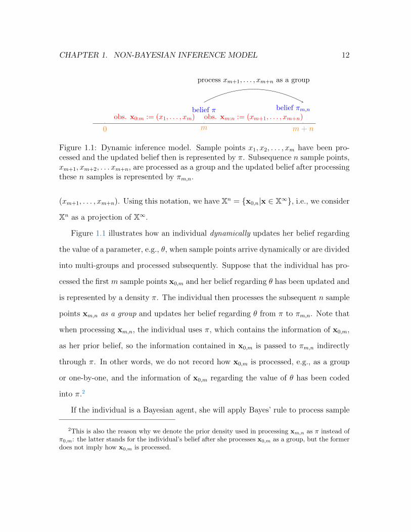
Figure 1.1: Dynamic inference model. Sample points x1, x2, . . . , xm have been pro-cessed and the updated belief then is represented by π. Subsequence n sample points,xm+1, xm+2, . . . xm+n, are processed as a group and the updated belief after processingthese n samples is represented by πm,n.
(xm+1, . . . , xm+n). Using this notation, we have Xn = x0,n|x ∈ X∞, i.e., we consider
Xn as a projection of X∞.
Figure 1.1 illustrates how an individual dynamically updates her belief regarding
the value of a parameter, e.g., θ, when sample points arrive dynamically or are divided
into multi-groups and processed subsequently. Suppose that the individual has pro-
cessed the first m sample points x0,m and her belief regarding θ has been updated and
is represented by a density π. The individual then processes the subsequent n sample
points xm,n as a group and updates her belief regarding θ from π to πm,n. Note that
when processing xm,n, the individual uses π, which contains the information of x0,m,
as her prior belief, so the information contained in x0,m is passed to πm,n indirectly
through π. In other words, we do not record how x0,m is processed, e.g., as a group
or one-by-one, and the information of x0,m regarding the value of θ has been coded
into π.2
If the individual is a Bayesian agent, she will apply Bayes’ rule to process sample
2This is also the reason why we denote the prior density used in processing xm,n as π instead ofπ0,m: the latter stands for the individual’s belief after she processes x0,m as a group, but the formerdoes not imply how x0,m is processed.
CHAPTER 1. NON-BAYESIAN INFERENCE MODEL 13
points; i.e.,
πm,n(θ | x) =`m,n(θ|x)π(θ)∫
Θ`m,n(θ|x)π(θ)ν(dθ)
, θ ∈ Θ, (1.1)
where `m,n(θ|x) is the likelihood of θ given the first m sample points x0,m and the
subsequent n sample points xm,n. In other words, if she is using Bayes’ rule to
process xm,n as a whole, the posterior density πm,n, which stands for the agent’s
belief regarding θ after processing xm,n, is proportional to the likelihood of θ times
the prior density π, which stands for the agent’s belief regarding θ before processing
xm,n. In other words, π stands for the agent’s belief regarding θ after processing the
first m sample points, i.e., is the posterior density obtained by processing the first m
sample points.
In Bayesian theory, `m,n(θ|x) is nothing but the conditional probability density
of xm,n given θ and x0,m. Formally, for each parameter θ, a measure Πθ is defined
on X∞, representing the distribution of sample sequences under θ. Thus, we have
defined a mapping from Θ to the space of probability measures on X∞, which maps θ
to Πθ, and we assume this mapping to be one-to-one and measurable. It is commonly
assumed in the Bayesian literature that there exists a σ-finite measure νX on X such
that for any θ ∈ Θ and any n ≥ 1 the projection of Πθ onto Xn, which represents the
distributions of sample sequences of size n, is absolutely continuous with respect to
νnX , the product measure of νX on Xn. Then, `m,n(θ|x) is the density of the conditional
distribution of xm,n given θ and x0,m with respect to νnX .
When the individual believes that sample points are i.i.d. given parameter θ,
`m,n(θ|x) does not depend on x0,m. Nonetheless, πm,n in (1.1) still reflects the infor-
mation contained in x0,m because this information has been coded into π and thus
passed to πm,n.
CHAPTER 1. NON-BAYESIAN INFERENCE MODEL 14
Bayes’ rule (1.1) constitutes a rational model in the sense that the posterior density
is computed from a probabilistic model: the posterior density stands for the condi-
tional distribution of the unknown parameter given the observed samples. Given
the likelihood, however, Bayes’ rule can be regarded as a mapping from the space
of probability densities and sample sequences to the space of probability densities.
Formally, denote P(Θ) as the set of probability densities on Θ.3 Then, Bayes’ rule
can be represented by mappings IBm,n,m ≥ 0, n ≥ 1 from X∞×P(Θ) to P(Θ), where,
for each x ∈ X∞ and π ∈ P(Θ), πm,n(·|x) := IBm,n(x, π) is defined through (1.1).
Now, we propose a new inference model, named coherent inference model. Again,
suppose the individual has processed x0,m and her belief has been updated to π. She is
then processing subsequent sample points xm,n as a whole and her belief will become
πm,n afterwards. In the coherent inference model,
πm,n(θ|x) =qm,n(θ|x)gm(π(θ))∫
Θqm,n(θ|x)gm(π(θ))ν(dθ)
, θ ∈ Θ. (1.2)
We represent the coherent inference model as the set of mappings ICm,n, m ≥ 0, n ≥ 1
from X∞ × P(Θ) to P(Θ): For each x ∈ X∞ and π ∈ P(Θ), ICm,n(x, π) = πm,n(·|x)
where πm,n is defined as in (1.2).
We discuss the three key components of the coherent inference model one by one.
First, the model is dynamic, consisting of mappings indexed by m and n. Here, m
stands for the number of sample points that have been processed previously and n
stands for the number of subsequent data points that are being processed as a whole.
The dynamic setting is necessary in order to study how different ways of processing
samples affect the inference of unknown parameters.
3One may replace P(Θ) with a subset of P(Θ). When all bounded densities with support onfinite-measured sets are under consideration, all the results in this chapter remain true.
CHAPTER 1. NON-BAYESIAN INFERENCE MODEL 15
Second, after processing x0,m, the individual’s belief is represented by π and it
is used as the prior belief when processing the subsequent sample points xm,n. A
distortion function gm is applied to the prior density π when processing xm,n. Note
that the distortion function does not depend on sample points, but it can depend on
m, i.e., the number of sample points that have been processed.
Third, qm,n(θ|x) is the pseudo-likelihood of θ given x0,m that has been processed
and xm,n that is being processed. The pseudo-likelihood can be regarded as the carrier
of the information of observed samples on parameters, but it can be different from
the likelihood in the Bayesian model.
In short, compared to the Bayesian model, the coherent inference model imposes
distortion on prior densities and replaces the likelihood with a pseudo-likelihood, so it
includes the Bayesian model as a special case. The coherent inference model, however,
does not have a probabilistic interpretation; it can only be understood as mappings
that take samples and prior densities as input and posterior densities as output. The
pseudo-likelihood qm,nm≥0,n≥1 and the distortion functions gmm≥0 can then be
regarded as the parameters of these mappings.
The motivation of the coherent inference model is two-fold: First, this model is
general enough to accommodate many non-Bayesian inference models in the literature
and to describe some non-Bayesian behavior; see the examples in Section 1.3. Second,
this model is a consequence of assuming coherence and separability. An inference
model is coherent if the resulting posterior density is indeed a probability density. In
the coherent inference model, with nonrestrictive assumptions on qm,n and gm that
we will present shortly, the posterior density πm,n satisfies πm,n(θ|x) ≥ 0,∀θ ∈ Θ and∫Θπm,n(θ|x)ν(dθ) = 1, showing that πm,n is a probability density. On the other hand,
CHAPTER 1. NON-BAYESIAN INFERENCE MODEL 16
in the coherent inference model, for any θ1, θ2 ∈ Θ, we have
πm,n(θ1|x)
πm,n(θ2|x)=qm,n(θ1|x)
qm,n(θ2|x)× gm(π(θ1))
gm(π(θ2)), (1.3)
provided the denominators are nonzero. Thus, the posterior odds of θ1 in favor of
θ2 are equal to the pseudo-likelihood ratio multiplied by the distorted prior odds.
In other words, the prior density and the observed sample determine the posterior
density separately.4
Before we proceed, we make the following assumption, which will be in force
throughout the paper.
Assumption 1 1. The number of elements of Θ is more than two and the support
of ν is Θ. Furthermore, Aµ := θ|ν(θ) > 0 is a closed set and ν has no
atom on Θ/Aµ.
2. For each m ≥ 0, gm is continuous and strictly increasing and satisfies gm(0) = 0.
3. For each m ≥ 0, n ≥ 1, (a) for each θ ∈ Θ, qm,n(θ|x) depends on x0,m+n only
and is measurable in x, and, for each x ∈ X∞, qm,n(θ|x) is continuous in θ;
and (b) for each x ∈ X∞, qm,n(θ|x) > 0 for ν-almost everywhere (a.e.) θ ∈ Θ
and∫
Θqm,n(θ|x)gm(π(θ))ν(dθ) < +∞ for any π ∈ P(Θ).
Let us comment on this assumption. Because in most inference problems Θ contains
4Coherence and separability may not always apply when individuals make inferences. Indeed,Marks and Clarkson [1972] and Teigen [1974] found that subjects’ estimates of posterior probabilitiesin their experiments were not coherent. Nevertheless, these two properties are convenient in inferencemodeling, and the coherent inference model satisfying them is general enough to accommodate manynon-Bayesian inference models, so we do not explore, in this chapter, cases in which these twoproperties fail. To have a model without the coherence property, one can generalize the coherentinference model by imposing distortion on posterior densities as well. Indeed, we can prove that thisgeneralized model is coherent if and only if there is no distortion on posterior densities; proofs canbe found in Appendix B.
CHAPTER 1. NON-BAYESIAN INFERENCE MODEL 17
more than two elements, for convenience we exclude the case in which Θ contains only
two elements.5 On the other hand, it is nonrestrictive to assume that the support of
ν is the whole space Θ. Otherwise, we can replace Θ with the support of ν because all
the prior distributions under consideration are dominated by ν. The set Aµ contains
all the singletons in Θ with positive measures, i.e., contains all the atoms of ν, and
is countable. Thus, it is nonrestrictive to assume that ν has no atom on Θ/Aν .
Assuming Aν to be closed is of technical importance, but it is not restrictive: in
many inference models, Aµ is either the empty set or Θ and thus is closed.
The monotonicity and continuity of gm are reasonable assumptions because this
function represents distortion on the prior density. On the other hand, gm(0) = 0 if
and only if πm,n(θ|x) = 0 for any θ ∈ Θ such that π(θ) = 0. Thus, the assumption
gm(0) = 0 essentially stipulates that if a particular θ is impossible under the prior
belief, then it is also impossible under the posterior belief.
Part 3-(a) of Assumption 1 is standard. On the other hand, to make the coherent
inference model (1.2) well-defined, we need to assume that 0 <∫
Θqm,n(θ|x)gm(π(θ))ν(dθ) <
+∞ for any prior density π and any sample x. Note that∫
Θqm,n(θ|x)gm(π(θ))ν(dθ) >
0 for any prior density π if and only if qm,n(θ|x) > 0 for ν-a.e. θ ∈ Θ. This assumption
is satisfied by many interesting examples; see Section 1.3.3.3. However, it also fails in
some cases. For instance, let Θ = [0, 1] and X = [0, 1], and for each θ ∈ Θ, samples
are i.i.d. and follow the uniform distribution on [0, θ]. Then, the likelihood function
5In some inference models, such as the model of confirmatory bias proposed by Rabin and Schrag[1999], Θ contains two elements θ1 and θ2 only. In this case, Proposition 1 still holds with condition(i) replaced by the one that gm(x)/gm(y) = g′m(x)/g′m(y) for any x, y > 0 such that xν(θ1) +yν(θ2) = 1. Theorem 1 still holds with condition (i) replaced by the one that gm(x)/gm(y) = x/yfor any x, y > 0 such that xν(θ1) + yν(θ2) = 1 and any m ≥ 1. In addition, Theorem 2 alsoholds with the condition that g0 is a linear function in part (i) of the theorem is replaced by the onethat g0(x)/g0(y) = x/y for any x, y > 0 such that xν(θ1) + yν(θ2) = 1. Note that the conditiongm(x)/gm(y) = x/y stipulates that the distortion gm does not affect the prior odds of θ1 in favor ofθ2. Note also that this condition does not imply that gm is a linear function. Proofs can be foundin Appendix C.

CHAPTER 1. NON-BAYESIAN INFERENCE MODEL 18
is 1θ1[0,θ](x). Given x, the likelihood is zero for θ ∈ [0, x).
It worth noting that the coherent inference model is general enough to nest many
existing non-Bayesian inference models and imply new models of conservatism and
base-rate neglect (see Section 1.3), but at the same time this model has its restrictions
on belief updating. Indeed, as discussed above, in the coherent inference model, the
prior density and the observed sample determine the posterior density separably. Due
to such separability, the distortion applied to the prior probability is independent of
the observed sample points. This is in contrast to the model proposed by Epstein
[2006] and the model proposed by Ortoleva [2012] in which the prior density in the
Bayes’ rule is replaced by another density that can depend on the observed sample
points.6 Another restriction of the coherent inference model is that an impossible
parameter value under the prior belief is also impossible under the posterior belief.
In the model proposed by Ortoleva [2012], however, an impossible event under the
initial prior belief chosen by the agent can become possible under the posterior belief
after observing a sample point.
Before we proceed, let us define the effective domain of gm. One can see that
the prior density, which appears as the argument of gm in the coherent inference
model (1.2), may not be able to take all nonnegative real values. For instance, if
Θ = θ1, . . . , θn and ν(θi) > 0, i = 1, . . . , n, the maximum value that a density
can take is max1/ν(θi)|i = 1, . . . , n. Therefore, in this case the definition of
6The preference models proposed by Epstein [2006] and by Ortoleva [2012] are based on severalaxioms of individuals’ preferences, so they cannot be directly compared to the coherence inferencemodel, which is a descriptive model of individuals’ inference behavior. The interpretation of thepreference models therein, however, suggests that these models can imply inference behavior thatcannot be nested in the coherent inference model. In the model proposed by Epstein [2006], theagent retroactively applies a posterior probability measure that can be arbitrary, and this measuremay not result from the coherent inference model. In the model proposed by Ortoleva [2012], theagent abandons the initial prior she chooses if this prior fails to pass a test. In this case, the agentchooses a new prior, and this choice depends on the observed sample points.
CHAPTER 1. NON-BAYESIAN INFERENCE MODEL 19
gm(z) for z beyond this maximum value is irrelevant, so the effective domain of gm is
from 0 to this maximum value. In general, one can see that the effective domain of
gm is [0,M ] ∩ [0,+∞), where M := max1/ν(θ)|θ ∈ Θ with 1/0 := +∞.
Proposition 1 For any fixed m ≥ 0 and n ≥ 1, consider two pairs of pseudo-
likelihood and distortion, (qm,n(θ|x), gm) and (q′m,n(θ|x), g′m), that satisfy Assumption
1. Then, (qm,n(θ|x), gm) and (q′m,n(θ|x), g′m) lead to the same posterior density πm,n
in the coherent inference model (1.2) for any prior density π and any sample sequence
x if and only if (i) there exists Cm > 0 such that gm(z) = Cmg′m(z) for all z in the
effective domain of gm and g′m, and (ii) for any x ∈ X∞, there exists Cm,n(x) > 0
such that qm,n(θ|x) = Cm,n(x)q′m,n(θ|x) for all θ ∈ Θ.
Proposition 1 shows that if the inference behavior of an individual can be rep-
resented by the coherent inference model (1.2), the distortion gm and the pseudo-
likelihood qm,n in this representation are uniquely determined up to a positive scaling
constant.
1.2.2 Processing Consistency
Imagine that the daily return rates of a stock are i.i.d. and the mean of the return
rates is to be estimated. Suppose the daily returns in the past ten days are available.
These daily returns can be processed in different ways to lead to the posterior estimate
of the mean. For instance, one investor processes the ten returns as a group, i.e.,
simultaneously, to obtain his posterior belief while another investor processes them
one by one, i.e., sequentially updates his belief after observing each return. In the
Bayesian model, these two methods of data-processing result in the same posterior
belief. However, this is not necessarily the case in the coherent inference model or in
other non-Bayesian models.
CHAPTER 1. NON-BAYESIAN INFERENCE MODEL 20
The issue of consistency across various methods of data-processing is also observed
by Benjamin et al. [2016] in the discussion of non-belief in the law of large numbers
(NBLLN). As mentioned by Benjamin et al. [2016], there is little experimental ev-
idence to show whether or not individuals are consistent when processing data in
different ways; the only published findings of which we are aware of are those of
Shu and Wu [2003] and Kraemer and Weber [2004], where the experimental results
indicate inconsistency.
If an individual is processing inconsistent when making an inference, various is-
sues can arise. In particular, it becomes relevant to model how the individual groups
the data she received; see a full discussion in Section 5 and Appendix A of Benjamin
et al. [2016].7 In this chapter, we attempt to provide a characterization of process-
ing consistency for the coherent inference model. Because of the various issues and
increased modeling complexity, such as the modeling of how individuals group and
process data, that arise from processing inconsistency, one might want to look for
a processing-consistent non-Bayesian inference model that is able to describe some
non-Bayesian behavior to some extent and at the same time retains tractability. In
this case, the characterization of processing consistency becomes useful.
We first define processing consistency formally:
Definition 1 The coherent inference model (1.2) is processing consistent if for each
m ≥ 1, n ≥ 1, any π ∈ P(Θ), and any x ∈ X∞,
π0,m+n(θ|x) = πm,n(θ|x), ν-a.e. θ ∈ Θ,
7We consider only the case in which the individual groups and processes the data retrospectively.Benjamin et al. [2016] consider also how the individual processes the data prospectively so as topredict them. Inconsistency can also arise when the individual predicts the data. Because we areonly concerned about inference, we focus on retrospective data processing.
CHAPTER 1. NON-BAYESIAN INFERENCE MODEL 21
where π0,m+n := IC0,m+n(x, π) and πm,n := ICm,n(x, IC0,m(x, π)).
According to Definition 1, if the coherent inference model is processing consistent,
then for any sample x0,m+n, processing the whole sample sequence simultaneously or
dividing the sequence into two groups x0,m and xm,n and processing them consecu-
tively will result in the same posterior distribution. One can see that dividing the
sequence into multiple groups and processing them consecutively will lead to the same
posterior distribution as well.
Note that here we assume samples points arrive or are arranged in order. An
individual can partition a sample sequence in multiple pieces but cannot shuffle the
sample points. This assumption is reasonable if the individual believes that the data
are the sample points of a time series. When the data are i.i.d. sample points, such
as the outcomes of repeated experiments, it is valid to discuss whether the individual
is processing consistent if she can even shuffle the sample points. In this chapter, we
focus on the case in which the individual cannot shuffle the sample points.
Theorem 1 The coherent inference model (1.2) is processing consistent if and only
if
(i) for each m ≥ 1, gm is a linear function in its effective domain, i.e., there exists
constant Km > 0 such that gm(z) = Kmz for all z in its effective domain; and
(ii) for each m ≥ 1 and n ≥ 1 and any x ∈ X∞, there exists Cm,n(x) > 0 such that
q0,m+n(θ|x) = Cm,n(x)q0,m(θ|x)qm,n(θ|x), ∀θ ∈ Θ. (1.4)
Let us explain conditions (i) and (ii) in Theorem 1 one by one. Condition (i)
stipulates that the density that is obtained after processing part of a sample se-
quence and used as the prior density when processing the subsequent parts of the
CHAPTER 1. NON-BAYESIAN INFERENCE MODEL 22
sequence cannot be distorted. To understand this condition, fix a sample sequence
x0,m+n and consider two scenarios of processing it: processing x0,m and xm,n subse-
quently and processing x0,m+n as a whole. The difference in the posterior densities
in these two scenarios arises from 1) the difference in the pseudo-likelihood, i.e.,
q0,m(θ|x)qm,n(θ|x)/q0,m+n(θ|x) and 2) the difference in whether or not distortion gm
is applied, i.e., gm(π0,m(θ|x)
)/π0,m(θ|x) is a constant or not. To have processing con-
sistency, these two sources of difference must offset each other. For fixed x0,m+n, the
difference in the pseudo-likelihood is also fixed, so the second source of difference,
i.e., gm(π0,m(θ|x)
)/π0,m(θ|x), should be the same for any initial prior density π0 (i.e.,
the individual’s belief before observing x0,m+n) and thus the same for any π0,m. In
consequence, gm must be a linear function.
To further understand condition (i), we consider Θ = 1/4, 1/2, 3/4 and i.i.d. 0-1
samples points such that the probability that each sample point takes value 1 is θ.
Assume the pseudo-likelihood in the coherent inference model to be the true likelihood
and gm(z) =√z, m ≥ 0. Suppose that two sample points, 0 and 1, are observed and
the prior density π0 before observing them is flat, i.e., π0(1/4) = π0(1/2) = π0(3/4) =
1/3. If the two sample points are processed as a group, then the posterior density is
π0,2(1/2) =1/4
(3/16) + (1/4) + (3/16)=
2
5, π0,2(1/4) = π0,2(3/4) =
3
10.
Intuitively, π0 is flat so the distortion applied on it has no effect. In consequence, the
two sample points indicate that θ = 1/2 is most likely. On the other hand, if the two
sample points are processed subsequently, then the belief after processing the first
sample point becomes
π0,1(1/4) =3/4
(3/4) + (1/2) + (1/4)=
1
2, π0,1(1/2) =
1
3, π0,1(3/4) =
1
6.
CHAPTER 1. NON-BAYESIAN INFERENCE MODEL 23
After processing the second sample point, the belief is further updated to
π0,2(1/4) =(1/4)
√1/2
(1/4)√
1/2 + (1/2)√
1/3 + (3/4)√
1/6=
√3√
3 + 2√
2 + 3,
π0,2(1/2) =2√
2√3 + 2
√2 + 3
, π0,2(3/4) =3√
3 + 2√
2 + 3.
Thus, when processing the two sample points separately, the individual believes that
θ = 3/4 is most likely. The intuition is as follows: when processing the two sample
points separately, the information of the first sample point, 0, is passed to the final
posterior density π0,2 through π0,1 and thus is discounted due to the distortion g1.
In consequence, the agent underestimates the information of the first sample point
0 and thus overestimates the chance of θ = 3/4. By contrast, when processing the
two sample points, 0 and 1, as a whole, their information is processed directly and
correctly, so the individual finds that θ = 1/2 is most likely.
We have showed that to have processing consistency, the density that is obtained
after processing a part of a sample sequence and used as the prior density when pro-
cessing the subsequent parts of the sequence cannot be distorted because it contains
the information of the sequence. Note, however, that the initial prior density before
processing any part of a sample sequence can be distorted because it does not contain
any information of the sample sequence. Indeed, distorting initial prior density π
with distortion function g0 is equivalent to using the following prior density without
distorting it:
π(θ) :=g0(π(θ))∫
Θg0(π(θ))ν(dθ)
, θ ∈ Θ. (1.5)
Thus, one cannot distinguish between the distortion and the use of a false prior
density.
CHAPTER 1. NON-BAYESIAN INFERENCE MODEL 24
Next, we explain part (ii) of the sufficient and necessary condition in Theorem
1, which is a product rule for the pseudo-likelihood. According to (1.2), the infor-
mation contained in x0,m+n determining the odds of θ1 in favor of θ2 is quantified
as the log pseudo-likelihood ratio log[q0,m+n(θ1|x)/q0,m+n(θ2|x)] if x0,m+n is processed
as a whole. On the other hand, when x0,m and xm,n are processed sequentially,
the information contained in x0,m is quantified as log[q0,m(θ1|x)/q0,m(θ2|x)] and the
information contained xm,n is quantified as log[qm,n(θ1|x)/qm,n(θ2|x)]. As already dis-
cussed, to achieve processing consistency, we cannot have distortion on the prior
density when processing xm,n. Consequently, the information contained in x0,m
is transferred without distortion in the determination of the posterior odds given
x0,m+n. As a result, the total information of x0,m+n is log[q0,m(θ1|x)/q0,m(θ2|x)] +
log[qm,n(θ1|x)/qm,n(θ2|x)]. To acheive processing consistency, this information should
be the same as log[q0,m+n(θ1|x)/q0,m+n(θ2|x)]. One can see that this is true for any
θ1 and θ2 if and only if the product rule (1.4) holds.
To summarize, an individual can manifest processing inconsistency for two reasons.
First, she believes that the information contained in a sample sequence regarding the
odds of a parameter value in favor of another one, which is subjectively measured
by the individual in the coherent inference model as the log pseudo-likelihood ratio
of these two parameter values, is not additive; i.e., the information contained in
the sample sequence as a whole is not equal to the aggregate information contained
in multiple pieces of the sequence that are processed sequentially. Second, when
processing a sample sequentially, the individual distorts the odds of a parameter
value in favor of another given part of the sample, and this leads indirectly to the
distortion of the sample information.
Finally, the Bayesian model is processing consistent because there is no distortion
on prior densities and the likelihood satisfies the product rule. Indeed, likelihood
CHAPTER 1. NON-BAYESIAN INFERENCE MODEL 25
`m,n(θ|x) stands for the conditional probability density of xm,n given θ and x0,m, so
it must satisfy the product rule as a result of the conditional probability formula.
1.3 Examples
1.3.1 False-Bayesian Models
If one replaces the true likelihood `m,n in the Bayesian model (1.1) with the likeli-
hood ˜m,n of a “false” model of the underlying stochastic process driving the random
samples, the resulting model is a special case of the coherent inference model and is
processing consistent. We call such a model a false-Bayesian model. It turns out that
many models in the literature fall in this category, as illustrated in the following.
Barberis et al. [1998] propose a model of predicting future dividend payments
from historical dividend payments in order to depict investors’ short-term under-
reaction and long-term over-reaction to market news and to explain the medium-term
momentum and long-term reversal of equity prices. The true underlying model of the
dividend payments is a random walk, but the investors believe that the dividend
payments follow a regime switching process with two modes, namely, mean reverting
and trend following. Assuming the investors to believe in this false model, the authors
are able to explain the momentum and reversal effects. Although the model proposed
by Barberis et al. [1998] does not involve the inference of model parameters, the use
of a false model is in the same flavor of a false-Bayesian inference model.
Rabin [2002] proposes a false-Bayesian inference model for the law of small num-
bers. More precisely, an urn contains red balls and blue balls and the percentage
of red balls θ is the parameter to infer after a sequence of balls is drawn, with re-
placement, from the urn. Therefore, the true underlying model of the drawn balls
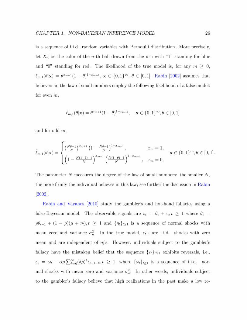
CHAPTER 1. NON-BAYESIAN INFERENCE MODEL 26
is a sequence of i.i.d. random variables with Bernoulli distribution. More precisely,
let Xn be the color of the n-th ball drawn from the urn with “1” standing for blue
and “0” standing for red. The likelihood of the true model is, for any m ≥ 0,
`m,1(θ|x) = θxm+1(1 − θ)1−xm+1 , x ∈ 0, 1∞, θ ∈ [0, 1]. Rabin [2002] assumes that
believers in the law of small numbers employ the following likelihood of a false model:
for even m,
˜m,1(θ|x) = θxm+1(1− θ)1−xm+1 , x ∈ 0, 1∞, θ ∈ [0, 1]
and for odd m,
˜m,1(θ|x) =
(Nθ−1N
)xm+1(1− Nθ−1
N
)1−xm+1, xm = 1,(
1− N(1−θ)−1N
)xm+1(N(1−θ)−1
N
)1−xm+1
, xm = 0,
x ∈ 0, 1∞, θ ∈ [0, 1].
The parameter N measures the degree of the law of small numbers: the smaller N ,
the more firmly the individual believes in this law; see further the discussion in Rabin
[2002].
Rabin and Vayanos [2010] study the gambler’s and hot-hand fallacies using a
false-Bayesian model. The observable signals are st = θt + εt, t ≥ 1 where θt =
ρθt−1 + (1 − ρ)(µ + ηt), t ≥ 1 and ηtt≥1 is a sequence of normal shocks with
mean zero and variance σ2η. In the true model, εt’s are i.i.d. shocks with zero
mean and are independent of ηt’s. However, individuals subject to the gambler’s
fallacy have the mistaken belief that the sequence εtt≥1 exhibits reversals, i.e.,
εt = ωt − αρ∑∞
k=0(δρ)kεt−1−k, t ≥ 1, where ωtt≥1 is a sequence of i.i.d. nor-
mal shocks with mean zero and variance σ2ω. In other words, individuals subject
to the gambler’s fallacy believe that high realizations in the past make a low re-
CHAPTER 1. NON-BAYESIAN INFERENCE MODEL 27
alization more likely today. The parameter α measures the strength of the gam-
bler’s fallacy and δ measures the relative influence of recent realizations. Note that
the observable signals take values in X := R. The parameter to be estimated is
θ := (ρ, µ, σ2η, σ
2ω) ∈ Θ := [0, 1] × R × R+ × R+. Using Kalman filtering, the likeli-
hoods of the true model and of the false model can be computed explicitly and are
actually normal densities.
1.3.2 Model of Base-Rate Neglect
Base-rate neglect is the tendency to overlook base rates, i.e., prior probabilities;
see for instance Bar-Hillel [1980, 1983]. Although base-rate neglect is related to the
representativeness heuristic [Tversky and Kahneman, 1974], the former is not neces-
sarily caused by the latter. In addition, although in some situations base-rate neglect
can be explained by the confusion between posterior probabilities and conditional
probabilities (i.e., likelihood), not all experimental results showing base-rate neglect
can be accounted for by such a confusion. There are many factors that contribute
to base-rate neglect, such as causality, specificity, and vividness; see the detailed
discussion in Bar-Hillel [1983].
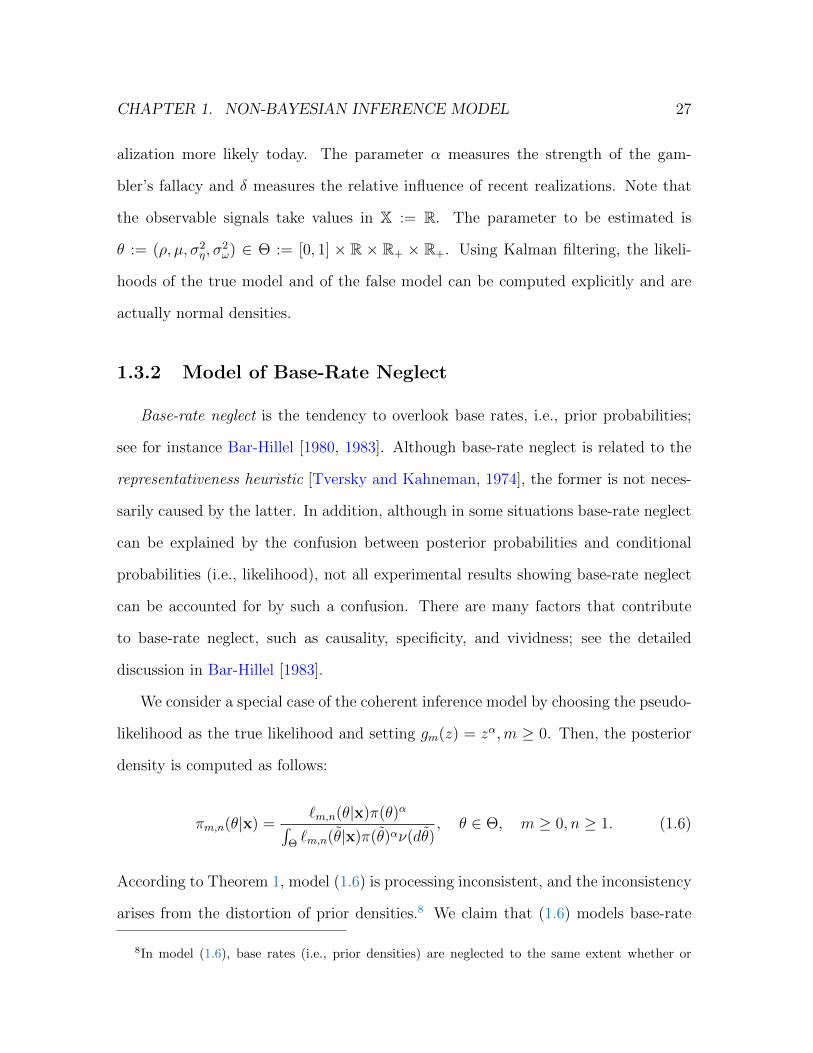
We consider a special case of the coherent inference model by choosing the pseudo-
likelihood as the true likelihood and setting gm(z) = zα,m ≥ 0. Then, the posterior
density is computed as follows:
πm,n(θ|x) =`m,n(θ|x)π(θ)α∫
Θ`m,n(θ|x)π(θ)αν(dθ)
, θ ∈ Θ, m ≥ 0, n ≥ 1. (1.6)
According to Theorem 1, model (1.6) is processing inconsistent, and the inconsistency
arises from the distortion of prior densities.8 We claim that (1.6) models base-rate
8In model (1.6), base rates (i.e., prior densities) are neglected to the same extent whether or
CHAPTER 1. NON-BAYESIAN INFERENCE MODEL 28
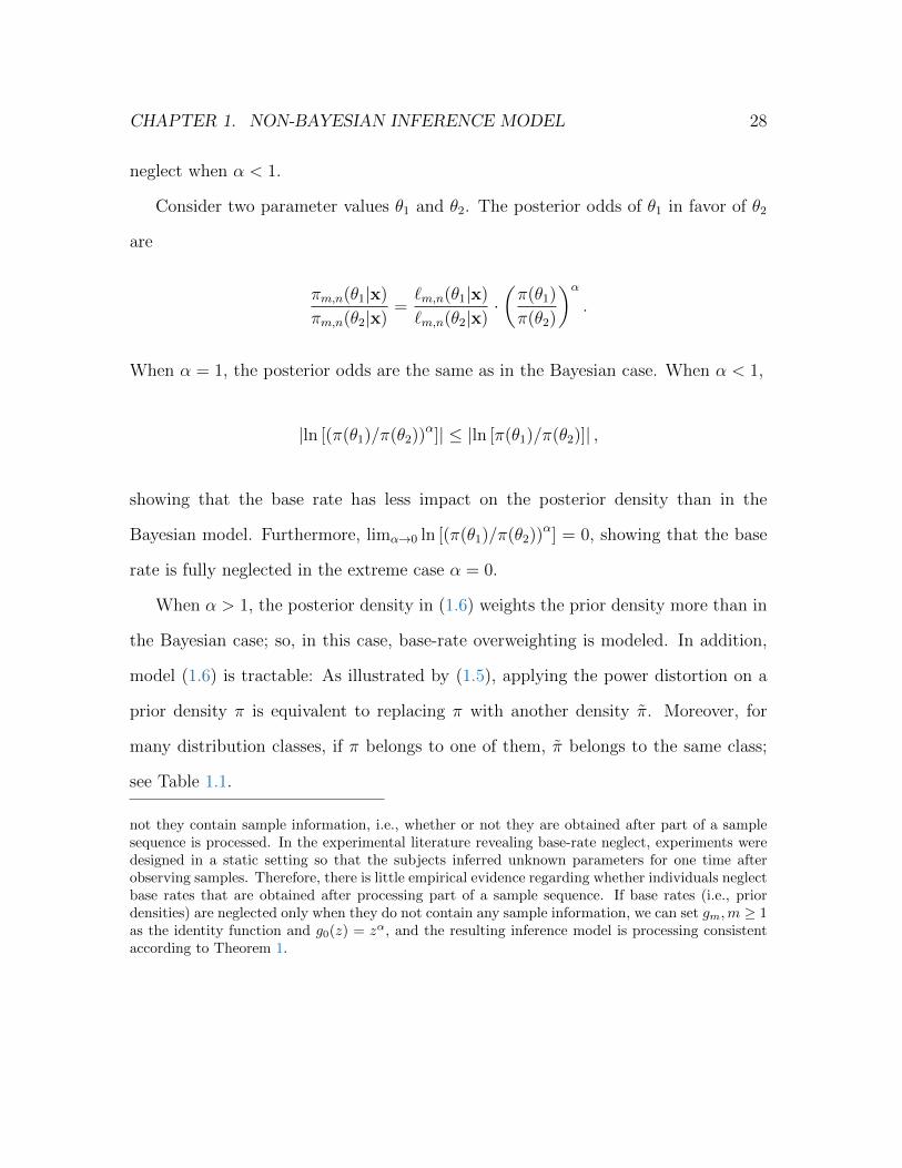
neglect when α < 1.
Consider two parameter values θ1 and θ2. The posterior odds of θ1 in favor of θ2
are
πm,n(θ1|x)
πm,n(θ2|x)=`m,n(θ1|x)
`m,n(θ2|x)·(π(θ1)
π(θ2)
)α.
When α = 1, the posterior odds are the same as in the Bayesian case. When α < 1,
|ln [(π(θ1)/π(θ2))α]| ≤ |ln [π(θ1)/π(θ2)]| ,
showing that the base rate has less impact on the posterior density than in the
Bayesian model. Furthermore, limα→0 ln [(π(θ1)/π(θ2))α] = 0, showing that the base
rate is fully neglected in the extreme case α = 0.
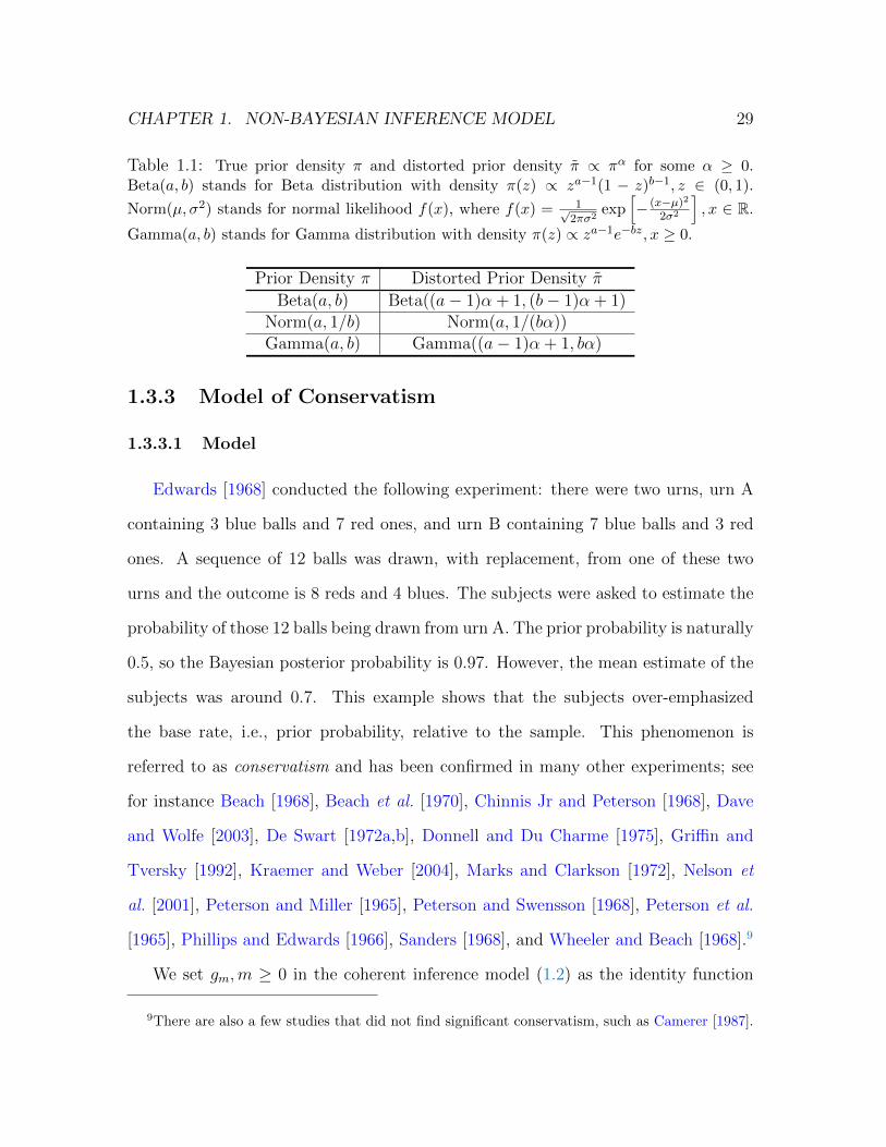
When α > 1, the posterior density in (1.6) weights the prior density more than in
the Bayesian case; so, in this case, base-rate overweighting is modeled. In addition,
model (1.6) is tractable: As illustrated by (1.5), applying the power distortion on a
prior density π is equivalent to replacing π with another density π. Moreover, for
many distribution classes, if π belongs to one of them, π belongs to the same class;
see Table 1.1.
not they contain sample information, i.e., whether or not they are obtained after part of a samplesequence is processed. In the experimental literature revealing base-rate neglect, experiments weredesigned in a static setting so that the subjects inferred unknown parameters for one time afterobserving samples. Therefore, there is little empirical evidence regarding whether individuals neglectbase rates that are obtained after processing part of a sample sequence. If base rates (i.e., priordensities) are neglected only when they do not contain any sample information, we can set gm,m ≥ 1as the identity function and g0(z) = zα, and the resulting inference model is processing consistentaccording to Theorem 1.
CHAPTER 1. NON-BAYESIAN INFERENCE MODEL 29
Table 1.1: True prior density π and distorted prior density π ∝ πα for some α ≥ 0.Beta(a, b) stands for Beta distribution with density π(z) ∝ za−1(1 − z)b−1, z ∈ (0, 1).
Norm(µ, σ2) stands for normal likelihood f(x), where f(x) = 1√2πσ2
exp[− (x−µ)2
2σ2
], x ∈ R.
Gamma(a, b) stands for Gamma distribution with density π(z) ∝ za−1e−bz, x ≥ 0.
Prior Density π Distorted Prior Density π
Beta(a, b) Beta((a− 1)α + 1, (b− 1)α + 1)Norm(a, 1/b) Norm(a, 1/(bα))Gamma(a, b) Gamma((a− 1)α + 1, bα)
1.3.3 Model of Conservatism
1.3.3.1 Model
Edwards [1968] conducted the following experiment: there were two urns, urn A
containing 3 blue balls and 7 red ones, and urn B containing 7 blue balls and 3 red
ones. A sequence of 12 balls was drawn, with replacement, from one of these two
urns and the outcome is 8 reds and 4 blues. The subjects were asked to estimate the
probability of those 12 balls being drawn from urn A. The prior probability is naturally
0.5, so the Bayesian posterior probability is 0.97. However, the mean estimate of the
subjects was around 0.7. This example shows that the subjects over-emphasized
the base rate, i.e., prior probability, relative to the sample. This phenomenon is
referred to as conservatism and has been confirmed in many other experiments; see
for instance Beach [1968], Beach et al. [1970], Chinnis Jr and Peterson [1968], Dave
and Wolfe [2003], De Swart [1972a,b], Donnell and Du Charme [1975], Griffin and
Tversky [1992], Kraemer and Weber [2004], Marks and Clarkson [1972], Nelson et
al. [2001], Peterson and Miller [1965], Peterson and Swensson [1968], Peterson et al.
[1965], Phillips and Edwards [1966], Sanders [1968], and Wheeler and Beach [1968].9
We set gm,m ≥ 0 in the coherent inference model (1.2) as the identity function
9There are also a few studies that did not find significant conservatism, such as Camerer [1987].
CHAPTER 1. NON-BAYESIAN INFERENCE MODEL 30
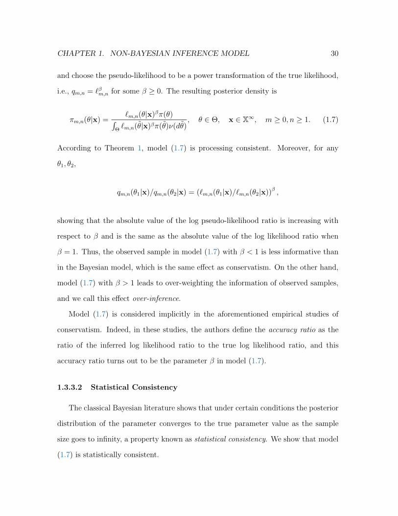
and choose the pseudo-likelihood to be a power transformation of the true likelihood,
i.e., qm,n = `βm,n for some β ≥ 0. The resulting posterior density is
πm,n(θ|x) =`m,n(θ|x)βπ(θ)∫
Θ`m,n(θ|x)βπ(θ)ν(dθ)
, θ ∈ Θ, x ∈ X∞, m ≥ 0, n ≥ 1. (1.7)
According to Theorem 1, model (1.7) is processing consistent. Moreover, for any
θ1, θ2,
qm,n(θ1|x)/qm,n(θ2|x) = (`m,n(θ1|x)/`m,n(θ2|x))β ,
showing that the absolute value of the log pseudo-likelihood ratio is increasing with
respect to β and is the same as the absolute value of the log likelihood ratio when
β = 1. Thus, the observed sample in model (1.7) with β < 1 is less informative than
in the Bayesian model, which is the same effect as conservatism. On the other hand,
model (1.7) with β > 1 leads to over-weighting the information of observed samples,
and we call this effect over-inference.
Model (1.7) is considered implicitly in the aforementioned empirical studies of
conservatism. Indeed, in these studies, the authors define the accuracy ratio as the
ratio of the inferred log likelihood ratio to the true log likelihood ratio, and this
accuracy ratio turns out to be the parameter β in model (1.7).
1.3.3.2 Statistical Consistency
The classical Bayesian literature shows that under certain conditions the posterior
distribution of the parameter converges to the true parameter value as the sample
size goes to infinity, a property known as statistical consistency. We show that model
(1.7) is statistically consistent.
CHAPTER 1. NON-BAYESIAN INFERENCE MODEL 31
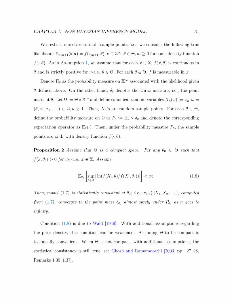
We restrict ourselves to i.i.d. sample points; i.e., we consider the following true
likelihood: `m,m+1(θ|x) = f(xm+1, θ),x ∈ X∞, θ ∈ Θ,m ≥ 0 for some density function
f(·, θ). As in Assumption 1, we assume that for each x ∈ X, f(x, θ) is continuous in
θ and is strictly positive for ν-a.e. θ ∈ Θ. For each θ ∈ Θ, f is measurable in x.
Denote Πθ as the probability measure on X∞ associated with the likelihood given
θ defined above. On the other hand, δθ denotes the Dirac measure, i.e., the point
mass, at θ. Let Ω := Θ×X∞ and define canonical random variables Xn(ω) := xn, ω =
(θ, x1, x2, . . . ) ∈ Ω, n ≥ 1. Then, Xn’s are random sample points. For each θ ∈ Θ,
define the probability measure on Ω as Pθ := Πθ × δθ and denote the corresponding
expectation operator as Eθ(·). Then, under the probability measure Pθ, the sample
points are i.i.d. with density function f(·, θ).
Proposition 2 Assume that Θ is a compact space. Fix any θ0 ∈ Θ such that
f(x, θ0) > 0 for νX-a.e. x ∈ X. Assume
Eθ0[supθ∈Θ| ln(f(Xi, θ)/f(Xi, θ0))|
]<∞. (1.8)
Then, model (1.7) is statistically consistent at θ0; i.e., π0,n(·|X1, X2, . . . ), computed
from (1.7), converges to the point mass δθ0 almost surely under Pθ0 as n goes to
infinity.
Condition (1.8) is due to Wald [1949]. With additional assumptions regarding
the prior density, this condition can be weakened. Assuming Θ to be compact is
technically convenient. When Θ is not compact, with additional assumptions, the
statistical consistency is still true; see Ghosh and Ramamoorthi [2003, pp. 27–28,
Remarks 1.35–1.37].
CHAPTER 1. NON-BAYESIAN INFERENCE MODEL 32
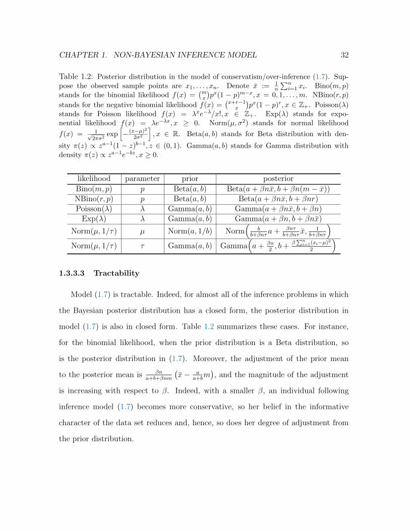
Table 1.2: Posterior distribution in the model of conservatism/over-inference (1.7). Sup-pose the observed sample points are x1, . . . , xn. Denote x := 1
n
∑ni=1 xi. Bino(m, p)
stands for the binomial likelihood f(x) =(mx
)px(1 − p)m−x, x = 0, 1, . . . ,m. NBino(r, p)
stands for the negative binomial likelihood f(x) =(x+r−1x
)px(1 − p)r, x ∈ Z+. Poisson(λ)
stands for Poisson likelihood f(x) = λxe−λ/x!, x ∈ Z+. Exp(λ) stands for expo-nential likelihood f(x) = λe−λx, x ≥ 0. Norm(µ, σ2) stands for normal likelihood
f(x) = 1√2πσ2
exp[− (x−µ)2
2σ2
], x ∈ R. Beta(a, b) stands for Beta distribution with den-
sity π(z) ∝ za−1(1 − z)b−1, z ∈ (0, 1). Gamma(a, b) stands for Gamma distribution withdensity π(z) ∝ za−1e−bz, x ≥ 0.
likelihood parameter prior posterior
Bino(m, p) p Beta(a, b) Beta(a+ βnx, b+ βn(m− x))NBino(r, p) p Beta(a, b) Beta(a+ βnx, b+ βnr)Poisson(λ) λ Gamma(a, b) Gamma(a+ βnx, b+ βn)
Exp(λ) λ Gamma(a, b) Gamma(a+ βn, b+ βnx)
Norm(µ, 1/τ) µ Norm(a, 1/b) Norm(
bb+βnτ
a+ βnτb+βnτ
x, 1b+βnτ
)Norm(µ, 1/τ) τ Gamma(a, b) Gamma
(a+ βn
2, b+
β∑ni=1(xi−µ)2
2
)1.3.3.3 Tractability
Model (1.7) is tractable. Indeed, for almost all of the inference problems in which
the Bayesian posterior distribution has a closed form, the posterior distribution in
model (1.7) is also in closed form. Table 1.2 summarizes these cases. For instance,
for the binomial likelihood, when the prior distribution is a Beta distribution, so
is the posterior distribution in (1.7). Moreover, the adjustment of the prior mean
to the posterior mean is βna+b+βnm
(x− a
a+bm), and the magnitude of the adjustment
is increasing with respect to β. Indeed, with a smaller β, an individual following
inference model (1.7) becomes more conservative, so her belief in the informative
character of the data set reduces and, hence, so does her degree of adjustment from
the prior distribution.
CHAPTER 1. NON-BAYESIAN INFERENCE MODEL 33
1.3.3.4 Comparison to the Literature
Several models of conservatism have been proposed in the literature. Rabin [2002]
proposes a false-Bayesian model of the law of small numbers. In this model, the sam-
ples are i.i.d. Bernoulli signals (taking either value a or value b), and the probability
of a signal taking value a is to be estimated. When the observed sample contains the
same number of a’s and b’s, Rabin [2002, Proposition 2] shows that conservatism is
present as a result of the law of small numbers.
In the model of NBLLN by Benjamin et al. [2016], on average, the agent with
NBLLN will under-infer when the sample size is larger than one, thus showing con-
servatism. However, under certain realizations, the agent may over-infer from the
samples.10
Unlike the models proposed by Rabin [2002] and Benjamin et al. [2016], the in-
ference model (1.7) with β < 1 leads to under-inference from samples, i.e., to con-
servatism, under all realizations. Let us emphasize that empirical findings show that
individuals do not under-infer in any realization and, indeed, in some situations they
over-infer. Thus, the models proposed by Rabin [2002] and Benjamin et al. [2016] are
descriptively more accurate than the conservatism model (1.7) in this chapter. We
regard our model as a convenient choice of conservatism modeling because it offers
tractability, as seen in Section 1.3.3.3, and because it separates conservatism from
other non-Bayesian behavior. Moreover, unlike the models of Rabin [2002] and Ben-
jamin et al. [2016], which can be applied only to i.i.d. Bernoulli samples, our model
can be applied to all types of samples.
10Although the models proposed by Rabin [2002] and Benjamin et al. [2016] can imply under-inference under certain realizations, these two models are more than describing conservatism. Indeed,they capture two fundamental non-Bayesian behaviors in inference, i.e., the law of small numberand the non-belief in the law of large number. Under-inference can be regarded as a consequence ofthese two behaviors.
CHAPTER 1. NON-BAYESIAN INFERENCE MODEL 34
Based on the decision-theoretic models proposed by Epstein [2006] and Epstein
et al. [2008], Epstein et al. [2010] consider non-Bayesian belief updating due to in-
dividuals’ over-weighting of prior beliefs, and thus to their under-reacting to new
samples, which they designate as under-reaction. These authors also consider the
opposite of under-reaction, namely over-reaction. Note that under-reaction is sim-
ilar to conservatism, while over-reaction is similar to over-inference in the context
of our investigation. Epstein et al. [2010] propose the following model of under-
reaction/over-reaction: the posterior distribution Πt+1 at time t + 1 is calculated as
Πt+1 = (1 − γt)BU(Πt;xt+1) + γtΠt, where Πt is the belief in the previous period
(i.e., at time t), xt+1 is the sample observed in the current period, BU(Πt;xt+1) is
the Bayesian posterior belief obtained from Πt and xt+1, and γt is a number less than
or equal to one. In other words, the posterior distribution is a weighted average of
the Bayesian posterior belief and the prior distribution. When γt = 0, this model
becomes a Bayesian model. When γt < 0, the posterior distribution places excess
weight on the Bayesian posterior, so over-reaction is modeled. When 0 < γt ≤ 1,
excess weight is placed on the prior distribution, so under-reaction is modeled.
Our model of conservatism/over-inference differs from and has some advantage
over the model proposed by Epstein et al. [2010]. First, our model has tractability
in the computation of posterior distributions, but theirs does not. For instance,
consider i.i.d. 0-1 Bernoulli samples with the probability of the sample taking 1 to
be estimated. If we assume the prior distribution to be a Beta distribution, then
the Bayesian posterior is also a Beta distribution. However, a linear combination of
two Beta distributions does not belong to any known distribution class. Secondly,
the output of our model is always a probability density, while γt in their model must
not be excessively negative so that Πt+1 remains a probability measure, and such
restriction is too tight in some applications. For instance, consider i.i.d. normal
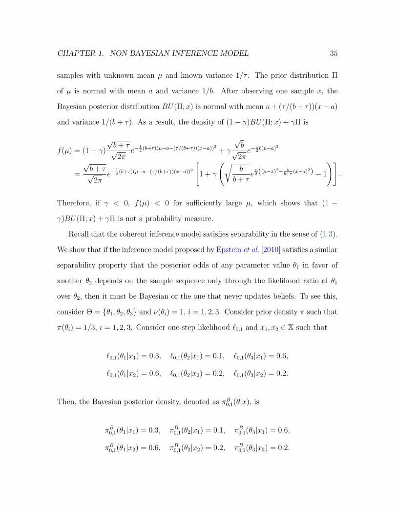
CHAPTER 1. NON-BAYESIAN INFERENCE MODEL 35
samples with unknown mean µ and known variance 1/τ . The prior distribution Π
of µ is normal with mean a and variance 1/b. After observing one sample x, the
Bayesian posterior distribution BU(Π;x) is normal with mean a+ (τ/(b+ τ))(x− a)
and variance 1/(b+ τ). As a result, the density of (1− γ)BU(Π;x) + γΠ is
f(µ) = (1− γ)
√b+ τ√2π
e−12
(b+τ)(µ−a−(τ/(b+τ))(x−a))2 + γ
√b√
2πe−
12b(µ−a)2
=
√b+ τ√2π
e−12
(b+τ)(µ−a−(τ/(b+τ))(x−a))2
[1 + γ
(√b
b+ τeτ2 ((µ−x)2− b
b+τ(x−a)2) − 1
)].
Therefore, if γ < 0, f(µ) < 0 for sufficiently large µ, which shows that (1 −
γ)BU(Π;x) + γΠ is not a probability measure.
Recall that the coherent inference model satisfies separability in the sense of (1.3).
We show that if the inference model proposed by Epstein et al. [2010] satisfies a similar
separability property that the posterior odds of any parameter value θ1 in favor of
another θ2 depends on the sample sequence only through the likelihood ratio of θ1
over θ2, then it must be Bayesian or the one that never updates beliefs. To see this,
consider Θ = θ1, θ2, θ3 and ν(θi) = 1, i = 1, 2, 3. Consider prior density π such that
π(θi) = 1/3, i = 1, 2, 3. Consider one-step likelihood `0,1 and x1, x2 ∈ X such that
`0,1(θ1|x1) = 0.3, `0,1(θ2|x1) = 0.1, `0,1(θ3|x1) = 0.6,
`0,1(θ1|x2) = 0.6, `0,1(θ2|x2) = 0.2, `0,1(θ3|x2) = 0.2.
Then, the Bayesian posterior density, denoted as πB0,1(θ|x), is
πB0,1(θ1|x1) = 0.3, πB0,1(θ2|x1) = 0.1, πB0,1(θ3|x1) = 0.6,
πB0,1(θ1|x2) = 0.6, πB0,1(θ2|x2) = 0.2, πB0,1(θ3|x2) = 0.2.
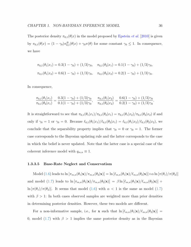
CHAPTER 1. NON-BAYESIAN INFERENCE MODEL 36
The posterior density π0,1(θ|x) in the model proposed by Epstein et al. [2010] is given
by π0,1(θ|x) = (1 − γ0)πB0,1(θ|x) + γ0π(θ) for some constant γ0 ≤ 1. In consequence,
we have
π0,1(θ1|x1) = 0.3(1− γ0) + (1/3)γ0, π0,1(θ2|x1) = 0.1(1− γ0) + (1/3)γ0,
π0,1(θ1|x2) = 0.6(1− γ0) + (1/3)γ0, π0,1(θ2|x2) = 0.2(1− γ0) + (1/3)γ0.
In consequence,
π0,1(θ1|x1)
π0,1(θ2|x1)=
0.3(1− γ0) + (1/3)γ0
0.1(1− γ0) + (1/3)γ0
,π0,1(θ1|x2)
π0,1(θ2|x2)=
0.6(1− γ0) + (1/3)γ0
0.2(1− γ0) + (1/3)γ0
.
It is straightforward to see that π0,1(θ1|x1)/π0,1(θ2|x1) = π0,1(θ1|x2)/π0,1(θ2|x2) if and
only if γ0 = 1 or γ0 = 0. Because `0,1(θ1|x1)/`0,1(θ2|x1) = `0,1(θ1|x2)/`0,1(θ2|x2), we
conclude that the separability property implies that γ0 = 0 or γ0 = 1. The former
case corresponds to the Bayesian updating rule and the latter corresponds to the case
in which the belief is never updated. Note that the latter case is a special case of the
coherent inference model with qm,n ≡ 1.
1.3.3.5 Base-Rate Neglect and Conservatism
Model (1.6) leads to ln [πm,n(θ1|x)/πm,n(θ2|x)] = ln [`m,n(θ1|x)/`m,n(θ2|x)]+α ln [π(θ1)/π(θ2)]
and model (1.7) leads to ln [πm,n(θ1|x)/πm,n(θ2|x)] = β ln [`m,n(θ1|x)/`m,n(θ2|x)] +
ln [π(θ1)/π(θ2)]. It seems that model (1.6) with α < 1 is the same as model (1.7)
with β > 1: In both cases observed samples are weighted more than prior densities
in determining posterior densities. However, these two models are different.
For a non-informative sample, i.e., for x such that ln [`m,n(θ1|x)/`m,n(θ2|x)] =
0, model (1.7) with β > 1 implies the same posterior density as in the Bayesian
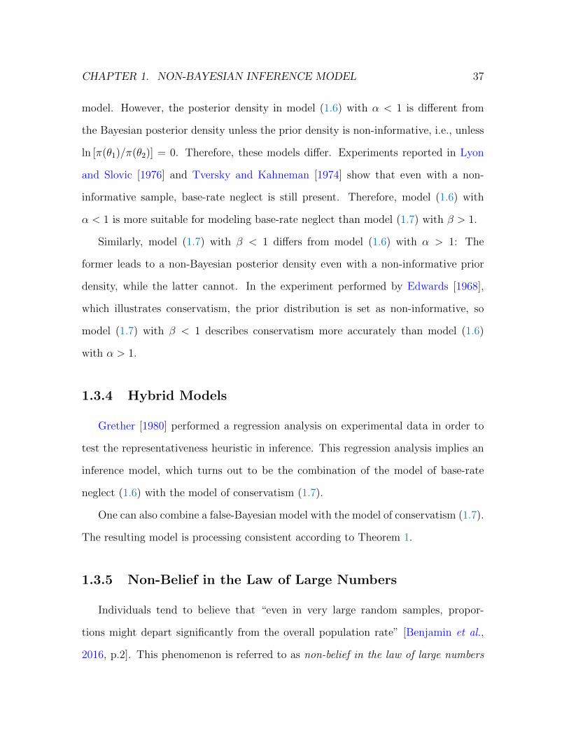
CHAPTER 1. NON-BAYESIAN INFERENCE MODEL 37
model. However, the posterior density in model (1.6) with α < 1 is different from
the Bayesian posterior density unless the prior density is non-informative, i.e., unless
ln [π(θ1)/π(θ2)] = 0. Therefore, these models differ. Experiments reported in Lyon
and Slovic [1976] and Tversky and Kahneman [1974] show that even with a non-
informative sample, base-rate neglect is still present. Therefore, model (1.6) with
α < 1 is more suitable for modeling base-rate neglect than model (1.7) with β > 1.
Similarly, model (1.7) with β < 1 differs from model (1.6) with α > 1: The
former leads to a non-Bayesian posterior density even with a non-informative prior
density, while the latter cannot. In the experiment performed by Edwards [1968],
which illustrates conservatism, the prior distribution is set as non-informative, so
model (1.7) with β < 1 describes conservatism more accurately than model (1.6)
with α > 1.
1.3.4 Hybrid Models
Grether [1980] performed a regression analysis on experimental data in order to
test the representativeness heuristic in inference. This regression analysis implies an
inference model, which turns out to be the combination of the model of base-rate
neglect (1.6) with the model of conservatism (1.7).
One can also combine a false-Bayesian model with the model of conservatism (1.7).
The resulting model is processing consistent according to Theorem 1.
1.3.5 Non-Belief in the Law of Large Numbers
Individuals tend to believe that “even in very large random samples, propor-
tions might depart significantly from the overall population rate” [Benjamin et al.,
2016, p.2]. This phenomenon is referred to as non-belief in the law of large numbers
CHAPTER 1. NON-BAYESIAN INFERENCE MODEL 38
(NBLLN) and is modeled in Benjamin et al. [2016].
In this model, the sample points are i.i.d. Bernoulli random variables, so X =
0, 1. The probability of a sample point taking value 1 is θ, which is to be inferred
from observed samples, so Θ = [0, 1]. The true likelihood is
`m,n(θ|x) =
[f
(1
n
m+n∑i=m+1
xi, θ
)]n, x ∈ X∞, θ ∈ Θ,m ≥ 0, n ≥ 1,
where f(a, θ) := θa(1 − θ)1−a. An individual with NBLLN believes in the following
pseudo-likelihood:
qm,n(θ|x) =
∫Θ
[f
(1
n
m+n∑i=m+1
xi, θ
)]nh(θ|θ)dθ, (1.9)
where, for each fixed θ, h(·|θ) is a probability density on Θ such that∫
Θθh(θ|θ)dθ = θ.
In other words, the individual pretends that the parameter value is a random variable
with mean θ. The individual then applies this pseudo-likelihood and sets gm,m ≥ 0
as the identity function in the coherent inference model (1.2) in order to calculate the
posterior density. This is the model of NBLLN proposed by Benjamin et al. [2016].
Benjamin et al. [2016] observe that the model of NBLLN is processing inconsistent.
The authors thus discuss several plausible ways of grouping samples; see discussions
in Benjamin et al. [2016]. With the help of the sufficient and necessary condition in
Theorem 1, we are able to prove the processing inconsistency of the model of NBLLN
for any density h(·|θ).
Proposition 3 The model of NBLLN is not processing consistent.
Note that prior densities are not distorted in the model of NBLLN. Thus, the pro-
cessing inconsistency of this model arises because the pseudo-likelihood does not sat-
CHAPTER 1. NON-BAYESIAN INFERENCE MODEL 39
isfy the product rule (1.4), i.e., because sample information contained in the pseudo-
likelihood is not additive.
1.4 Processing Consistency Does Not Imply Bayes’
Rule
We have shown that false-Bayesian models are processing consistent because
Bayes’ rule is applied in these models. Next, we study whether a processing-consistent
inference model is false Bayesian. It is interesting to clarify whether processing con-
sistency fully characterizes Bayes’ rule and to draw out their difference if not.
Recall that we represent the coherent inference model (1.2) as a family of map-
pings ICm,nm≥0,n≥1. Similarly, we can represent a false-Bayesian model with a false
underlying stochastic model (with likelihood ˜m,n) as IBm,nm≥0,n≥1.
Definition 2 (i) The coherent inference model (1.2) is false Bayesian in the strong
sense if there exists a false-Bayesian model IBm,nm≥0,n≥1 such that ICm,n(x, π) =
IBm,n(x, π), m ≥ 0, n ≥ 1 for any x ∈ X∞ and π ∈ P(Θ).
(ii) The coherent inference model (1.2) is false Bayesian in the weak sense if, for any
π ∈ P(Θ), there exist a false-Bayesian model IBm,nm≥0,n≥1 and a false prior density
π ∈ P(Θ) such that ICm,n(x, π) = IBm,n(x, π), m ≥ 0, n ≥ 1 for any x ∈ X∞.
In most contexts, only one prior density is involved, and it is unobservable and sub-
jective. Thus, when an observer tries to tell whether an individual uses the Bayesian
model to make an inference, she has no knowledge of the prior density used by the
individual. In this case, if the coherent inference model is false Bayesian in the weak
sense, it cannot be distinguished from a false-Bayesian model. On the other hand,
the examination of whether the coherent inference model is false Bayesian in the
CHAPTER 1. NON-BAYESIAN INFERENCE MODEL 40
strong sense is of theoretical interest. In addition, this examination is relevant in
experimental contexts where prior densities can be controlled.
Theorem 2 Denote the one-step pseudo-likelihood qm,1(θ|x) in the coherent inference
model as qm,1(θ|x0,m, xm+1).
(i) The coherent inference model (1.2) is false Bayesian in the strong sense if and
only if it is processing consistent, g0 is a linear function in its effective domain,
and, for each m ≥ 0, there exists a measurable function ϕm(x0,m, x) > 0,x0,m ∈
Xm, x ∈ X such that
∫Xϕm(x0,m, x)qm,1(θ|x0,m, x)νX(dx) = 1, ν-a.e. θ ∈ Θ, ∀x0,m ∈ Xm.
(1.10)
(ii) The coherent inference model (1.2) is false Bayesian in the weak sense if and
only if it is processing consistent and, for each m ≥ 1, there exists a measurable
function ϕm(x0,m, x) > 0,x0,m ∈ Xm, x ∈ X such that (1.10) holds.
Theorem 2 provides sufficient and necessary conditions under which the coherent
inference model (1.2) is false Bayesian in both the strong and the weak sense. First,
in both cases, processing consistency is necessary. As a result, the posterior density
can be calculated by processing sample points one by one. Second, for the coherent
inference model to be false Bayesian, one must be able to recast the quasi-likelihood in
a way that it can be interpreted probabilistically. Mathematically, it means that the
one-step pseudo-likelihood can be normalized into a likelihood, which is equivalent
to condition (1.10). Third, if the coherent inference model is false Bayesian only in
the weak sense, the initial prior density can be distorted and the one-step pseudo-
likelihood used to process the first sample point can be arbitrary because the resulting
CHAPTER 1. NON-BAYESIAN INFERENCE MODEL 41
posterior density cannot be differentiated from one that is obtained by using a false
prior density. If the coherent inference model is false Bayesian in the strong sense,
however, it results in the same posterior density as a false Bayesian model for any
prior density. In consequence, the initial prior density cannot be distorted and one
must be able to interpret the one-step pseudo-likelihood used to process the first
sample point probabilistically.
Condition (1.10) is easy to verify, as the following two examples illustrate. More-
over, these two examples show that processing consistency does not imply a false-
Bayesian model even in the weak sense.
Example 1 Let X = 0, 1 and let the samples be i.i.d. Bernoulli random variables.
The probability of each sample point taking value 1 is θ ∈ Θ := [0, 1], which is to
be estimated. The measure νX defined on X is the discrete measure, i.e., νX(0) =
νX(1) = 1, and the measure ν on Θ is the Lebesgue measure. In this case, the true
likelihood is
`m,n(θ|x) = θ∑m+ni=m+1 xi(1− θ)n−
∑m+ni=m+1 xi , x ∈ X∞, θ ∈ [0, 1].
The pseudo-likelihood in model (1.7) then becomes
qm,n(θ|x) = `m,n(θ|x)β = θβ∑m+ni=m+1 xi(1− θ)β(n−
∑m+ni=m+1 xi), x ∈ X∞, θ ∈ [0, 1].
This model is processing consistent.
Suppose there exists ϕm(x0,m, x) such that∫X ϕm(x0,m, x)qm,1(θ|x0,m, x)νX(dx) =
1 for ν-a.e. θ ∈ Θ. Then, we have ϕm(x0,m, 1)θβ + ϕm(x0,m, 0)(1 − θ)β = 1 for
ν-a.e. θ ∈ Θ. This is impossible, so model (1.7) with Bernoulli likelihood, although
processing consistent, is not false Bayesian in the weak sense.

CHAPTER 1. NON-BAYESIAN INFERENCE MODEL 42
Example 2 Set X = R and set the samples to be i.i.d. normal random variables
with variance σ2 and mean θ ∈ Θ := R. The mean θ is to be estimated. Both νX
and ν are the Lebesgue measure. In this case, the true likelihood is
`m,n(θ|x) = (2πσ2)−n/2 exp
[− 1
2σ2
m+n∑i=m+1
(xi − θ)2
], x ∈ X∞, θ ∈ Θ.
The pseudo-likelihood in model (1.7) then becomes
qm,n(θ|x) = `m,n(θ|x)β = (2πσ2)−βn/2 exp
[− β
2σ2
m+n∑i=m+1
(xi − θ)2
], x ∈ X∞, θ ∈ Θ.
This model is false Bayesian in the strong sense. Indeed, g0 is the identify function
in this model, and, by choosing ϕm ≡ (2πσ2)(β−1)/2β1/2, we have
∫Xϕm(x0,m, x)qm,1(θ|x0,m, x)νX(dx) =
∫X(2πσ2/β)−1/2 exp
[−β(x− θ)2
2σ2
]νX(dx) = 1.
Therefore, according to Theorem 2, this model is false Bayesian in the strong sense.
Indeed, the likelihood of the corresponding false-Bayesian model is
˜m,1(θ|x) =
(2πσ2
β
)−1/2
exp
[−β(xm+1 − θ)2
2σ2
], x ∈ X∞, θ ∈ Θ.
In other words, given the mean θ, the variance of the sample changes from σ2 in the
true model to σ2/β in the false model.
Finally, if we apply a nonlinear distortion g0 to the prior density as well, the
resulting model is false Bayesian in the weak but not in the strong sense.
CHAPTER 1. NON-BAYESIAN INFERENCE MODEL 43
1.5 Conclusions
In this chapter we have proposed a dynamic coherent inference model that is
sufficiently general to include the existing non-Bayesian inference models as special
cases and to imply new models of base-rate neglect and conservatism. The coherent
inference model is constructed by distorting the prior density in Bayes’ rule and
replacing the likelihood with the pseudo-likelihood.
We have proved a sufficient and necessary condition under which the coherent
inference model is processing consistent, i.e., the posterior density in the model is
invariant to how the samples are grouped and processed. This condition can be
used to check whether an inference model is processing consistent and also helps us
to understand the causes of processing inconsistency: Individuals can be processing
inconsistent if they distort sample information indirectly through prior densities or if
they measure sample information in a non-additive way.
We have proved sufficient and necessary conditions for the coherent inference
model to be false Bayesian, i.e., to be obtained by applying Bayes’ rule to a false
stochastic model, both in the strong and in the weak sense. Moreover, we have
provided examples of inference models that are processing consistent but not false
Bayesian. As a result, we have shown that processing consistency does not imply
Bayes’ rule.
Chapter 2
Processing Consistency in
Prediction
2.1 Introduction
Inference refers to the process of inferring unknown parameters of a stochastic
model after observing sample points. Processing consistency in inference refers to the
property that the inference of the unknown parameters does not depend on however
the observed sample points are processed retrospectively. In many situations, individ-
uals need to process sample points prospectively before they are observed, a process
named prediction. For instance, when deciding whether to purchase a group of sample
points from some data vendor, an individual needs to predict the sample points he
might receive from the vendor. In the Chapter 1, we proposed a general framework
for non-Bayesian inference, named coherent inference model, and showed that this
inference model is processing consistent if and only if (i) the individual cannot distort
the prior density that is obtained by processing part of a sample sequence and (ii)
the information contained in a sample sequence is additive when the sequence is di-44
CHAPTER 2. PROCESSING CONSISTENCY IN PREDICTION 45
vided into multiple pieces. In this chapter, we study when an individual’s prediction
is processing consistent, i.e., when the individual’s prediction of a group of sample
points does not depend on how he processes them prospectively.
In a related work, Epstein and Le Breton [1993] show that a preference relation
that satisfies certain axioms on decision under risk and the so-called dynamic consis-
tency axiom must be represented by expected utility under a subjective probability
measure, and this implies that the individual with this preference relation must use
the Bayes’ rule to update his belief. Our study is different from theirs in that we do
not consider a decision-theoretic framework; indeed, we consider a setting in which
the agent can make non-Bayesian inferences. In another related work, Benjamin et
al. [2016] show that in the model of NBLLN, individuals are processing inconsistent
in prediction. Compared to their work, we consider a general framework of predic-
tion with unknown parameters and study the issue of processing consistency in this
framework.
Imagine that an investor believes that the monthly returns of a stock follow a
distribution with an unknown parameter, such as the mean of the return. The investor
wants to predict the stock return in the following month based on historical data.
Because he knows the distribution of the stock return as long as the parameter is
known, it is natural for him to first estimate the parameter using the historical data
and then use the estimate to predict the stock return in the following month. We
formalize the investor’s thinking as a general prediction model.
More precisely, we consider an individual who needs to predict incoming sample
points based on historical samples. The individual has a stochastic model for the dy-
namics of the sample points with a known parameter. In other words, the individuals
has a prediction model with known parameter for the sample points; i.e., given the
parameter value, the individual knows the distribution of the sample points. The in-
CHAPTER 2. PROCESSING CONSISTENCY IN PREDICTION 46
dividual also has an inference model for the parameter. The individual then predicts
incoming sample points by combining his inference model and prediction model with
known parameter, leading to a general prediction model.
In the above prediction model, at each time, the agent needs to process the histori-
cal sample points retrospectively so as to make an inference of the unknown parameter
and process the incoming sample points prospectively so as to predict these sample
points. Inconsistency can arise in both the retrospective data processing period and
the prospective data processing period; the former leads to inconsistency in inference
and the latter leads to inconsistency in prediction. In this chapter, we focus on the
issue of processing consistency in prediction. To single out this issue, we assume
that the individual uses a processing consistent inference model. More precisely, we
assume that the individuals uses the processing-consistent, coherent inference model
(1.2) when processing data retrospectively. Note that because of Theorem 1, this in-
ference model is fully characterized by quasi-likelihood and distortion of initial priors,
and the quasi-likelihood satisfies the product rule (1.4).
The main result in this chapter shows that the above prediction model is pro-
cessing consistent, i.e., the prediction of sample points do not depend on how they
are processed prospectively, if and only if the quasi-likelihood in the inference model
is proportional to likelihood implied by the stochastic model of the data process. In
other words, the prediction model is processing consistent if and only if the individual
uses the same likelihood in inference and prediction, which means that the prediction
model must be described by a probabilistic model and thus the individual uses Bayes’
update to predict sample points.
The above result shows that individuals must be processing inconsistent in pre-
diction when they do not use the Bayes’ rule. Given that non-Bayesian behavior
is commonly observed in experimental and field studies, our result shows that how-
CHAPTER 2. PROCESSING CONSISTENCY IN PREDICTION 47
ever individuals process sample points prospectively matters. Then, when applying
non-Bayesian prediction models, we need to specify the way of individuals processing
data, and in many situations, this depends on how individuals perceive the way that
the data is passed to them.
In the second part of this chapter, we consider a consumer choice model to study
the impact of conservatism on consumer choices. In this model, we need to describe
how individuals process data prospectively. More precisely, we consider a car selection
problem in which an agent decides between two car brands. The agent can choose
to purchase reviewer reports from Consumer Report to gain information about the
quality of the cars in these two brands. After receiving the data, the agent decides
which brand to choose. We consider two cases: in the first case, the agent decides
whether to purchase a fixed amount of reports at one time. In the second case,
the agent can purchase one report each time and decide when to stop purchasing
additional reports. In the first case, the agent perceives that he will receive certain
number of reports at one time, so when predicting these reports in order to assess
their values, he tends to process them as a group. In the second case, the agent
perceives that he will receive just one report every time, so he tends to process the
incoming reports one by one. In both cases, we find that when the agent becomes
more conservative, he tends to under-infer the quality of the cars from the purchased
reports and thus (i) are less likely to revise his initial assessment of the car quality
when deciding which car to choose and (ii) are less willing to pay of the reports.
2.2 Model
Following the setting in Chapter 1, we assume that sample points take values in a
topologically complete and separate metric space X. Denote Xn as the product space
CHAPTER 2. PROCESSING CONSISTENCY IN PREDICTION 48
of n copies of X, and denote X∞ as the product space of countably infinite copies of
X. Assume that there exists a σ-finite measure νX on X and denote νnX as the product
measure of νX on Xn. The sample distribution is parametrized by θ, which is in a
topologically complete and separate metric space Θ and is unknown. θ has a prior
distribution, and estimation of θ is achieved by computing the posterior distribution
of θ given an observed sample sequence. We consider only the distribution of θ that is
absolutely continuous with respect to a given σ−finite measure ν on Θ. As a result,
any distribution of θ can be characterized by its density π with respect to ν.
We consider the following dynamic prediction model: suppose the agent already
observed sample points x0,m := (x1, . . . , xm) and attempts to predict the following
n sample points xm,n := (xm+1, . . . , xm+n). We assume that the agent believes in a
stochastic model of the dynamics of the sample points parameterized by θ; conse-
quently, he knows the distribution of the sample points to arrive if he knows θ. The
agent also has an inference model for θ, which leads to a distribution θ based on the
sample points he already observed. Then, the agent combines the inference model and
the stochastic model to form the prediction of sample points to arrive. To study the is-
sue of the means of prospective data-processing on prediction, we further assume that
the agent is processing consistent when making the inference of θ. More precisely, we
assume that the inference of θ follows the coherent inference model in Chapter 1 and
is processing consistent. Consequently, we can simply denote the posterior density of
θ as πm(θ|x) without recording the means by which the agent processes x0,m (e.g., as
a group or one by one). Moreover, πm is associated with a quasi-likelihood function q
that satisfies the product rule as in (1.4) and a possibly distorted prior density π0; see
(1.5). On the other hand, given θ, the agent believes that the sample points follow
a stochastic process parameterized by θ. Consequently, given θ and x0,m, the agent
believes that the density of xm,n (with respect to νnX) is `m,n(θ|x). Note that given θ,
CHAPTER 2. PROCESSING CONSISTENCY IN PREDICTION 49
`m,n represents the conditional probability density of xm,n give x0,m, so when fixing x,
we can view `m,n as a likelihood function; consequently, ` satisfies the product rule.
Now, suppose the agent processes xm,n prospectively as a group, we assume that
his prediction of xm,n given x0,m is based on his inference of θ given x0,m and his
prediction of xm,n given x0,m and θ. More precisely, the agent predicts that the
density of xm,n is
µm,n(x) =
∫Θ
`m,n(θ|x)πm(θ|x)ν(dθ). (2.1)
It is clear that given x0,m, µm,n is a probability density on Xn.
Definition 3 Given a processing-consistent, coherent inference model πm associ-
ated with quasi-likelihood ratio qm,n and distortion g0(·) on initial priors π0, and
a likelihood function `m,n that is used for prediction with known parameters, the
prediction model (2.1) is processing consistent if for any m ≥ 0, n1 ≥ 1, n2 ≥ 1, any
initial prior π0 ∈ P(Θ), and any x ∈ X∞, we have
µm,n1+n2(x) = µm,n1(x)µm+n1,n2(x). (2.2)
Note that given x0,m, the left-hand side of (2.2) stands for the density of xm,n1+n2
that is predicted by the agent when he processes xm,n1+n2 as a group prospectively.
On the right-hand side, µm,n1(x) stands for the density of xm,n1 conditioning on x0,m
that is predicted by the agent when he processes xm,n1 as a group prospectively.
Similarly, µm+n1,n2(x) stands for the density of xm+n1,n2 conditioning on x0,m+n1 that
is predicted by the agent when he processes xm+n1,n2 as a group prospectively. Thus,
the right-hand side of (2.2) represents the agent’s prediction of xm,n1+n2 when he
divides the sequence as two subsequences, xm,n1 and xm+n1,n2 , and process them
CHAPTER 2. PROCESSING CONSISTENCY IN PREDICTION 50
sequentially. Then, for the prediction model to be processing consistent, (2.1) needs
to hold for any x, π0, m, n1, and n2.
Let the following assumption be in force in this section:
Assumption 2 Suppose
(i) Assumption 1 holds.
(ii) The inference model is processing consistent; i.e., (i) and (ii) in Theorem 1
hold.
(iii) For each m ≥ 0, n ≥ 1, and x ∈ X∞, `m,n(θ|x) depends on x0,m+n only, is
continuous in θ, and `m,n(θ|x) > 0 for ν-almost everywhere (a.e.) θ ∈ Θ.
Moreover, for any ν-a.e. θ1 6= θ2, `m,n(θ1|x)/`m,n(θ2|x) is not a constant in x.
(iv) `m,n is a likelihood; i.e., `m,n satisfies the product rule (1.4) and
∫X`m,m+1(θ|x)νX(dxm,m+1) = 1, ∀θ ∈ Θ,x0,m ∈ Xm, m ≥ 0.
We have the following main theorem:
Theorem 3 The prediction model (2.1) is processing consistent if and only if for any
m ≥ 0, and x, there exists C0,m(x) > 0 such that
q0,m(θ|x) = C0,m(x)l0,m(θ|x). (2.3)
Note that when (2.3) holds, the inference πm is the same as the one obtained in a
Bayesian model with likelihood function to be `m,n. Consequently, Theorem 3 shows
that the prediction model is processing consistent if and only it is a Bayesian model,
i.e., if and only if µm,n is the conditional probability density of xm,n conditioning
CHAPTER 2. PROCESSING CONSISTENCY IN PREDICTION 51
on x0,m in the canonical probability space (Ω,F ,P), where Ω = X∞, F is the Borel
product of countably infinite copies the Borel σ-algebra of X, and
P =
∫Θ
Pθν(dθ),
where Pθ is the probability measure on (Ω,F) induced by the likelihood function
`m,n(θ|x).
2.3 Example: Normal Samples with Known Vari-
ance
Next, we illustrate Theorem 3 by an example. Suppose that the samples are i.i.d.
having normal distribution with unknown mean θ and known variance 1/τ . The prior
distribution of θ is Normal with mean a and variance 1/b. Suppose the agent uses
the model of conservatism/over-inference (1.7) to infer θ from sample points. Given
θ, the agent knows that the samples are i.i.d. and normally distributed with mean
θ and variance 1/τ . Then, the agent applies (2.1) to make predictions. Suppose
the agent already observed m sample points x1, . . . , xm and attempts to predict the
distribution of the following n sample points, xm+1, . . . , xm+n, as a group. Then,
according to Table 1.2, the posterior distribution of θ, denoted as πm, is normal
distribution with mean
b
b+ βmτa+
βmτ
b+ βmτx0,m,
CHAPTER 2. PROCESSING CONSISTENCY IN PREDICTION 52
where x0,m :=∑m
i=1 xi/m, and variance
1
b+ βmτ.
Consequently,
µm,n(x) =
∫Θ
`m,n(θ|x)πm(θ|x)dθ
=
∫Θ
(√τ
2π
)ne−
τ2
∑nj=1(xj−θ)2
√b+ βmτ
2πe−
b+βmτ2
(θ− bb+βmτ
a− βmτb+βmτ
x0,m)2dθ.
By the property of normal distribution, we conclude that µm,n(x) follows normal
distribution with mean vector
(b
b+ βmτa+
βmτ
b+ βmτx0,m
)1n,
where 1n stands for the n-dimensional column vector with all its components to be
1, and covariance matrix
1
b+ βmτ1n1
>n +
1
τIn,
where In stands for the n-dimensional identity matrix.
Now, suppose x0,m has already been observed and the agent predicts xm,n1+n2 by
processing it as a group, then, he believes that the distribution of xm,n1+n2 is
µm,n1+n2(x) ∼ N((
b
b+ βmτa+
βmτ
b+ βmτx0,m
)1n1+n2 ,
1
b+ βmτ1n1+n21
>n1+n2
+1
τIn1+n2
),
where N (d,C) denotes the normal distribution with mean vector d and covariance
matrix C. On the other hand, if the agent predicts xm,n1 first, which yields the
CHAPTER 2. PROCESSING CONSISTENCY IN PREDICTION 53
following distribution of xm,n1 given x0,m
µm,n1(x) ∼ N((
b
b+ βmτa+
βmτ
b+ βmτx0,m
)1n1 ,
1
b+ βmτ1n11
>n1
+1
τIn1
),
and then predicts xm+n1,n2 , which yields the following distribution of xm+n1,n2 given
x0,m+n1
µm+n1,n2(x) ∼ N((
b
b+ β(m+ n1)τa+
β(m+ n1)τ
b+ β(m+ n1)τx0,m+n1
)1n2 ,
1
b+ β(m+ n1)τ1n21
>n2
+1
τIn2
).
Consequently, when processing xm,n1 and xm+n1,n2 sequentially, the agent predicts
xm,n1+n2 , given x0,m, by the following distribution
µm,n1(x)µm+n1,n2(x) ∼ N((
b
b+ βmτa+
βmτ
b+ βmτx0,m
)1n1+n2 ,
1
b+ βmτ1n1+n21
>n1+n2
+1
τIn1+n2 −D
),
where
D =
0 1−βb+βmτ
1n11>n2,
1−βb+βmτ
1n21>n1, β(1−β)
(b+βmτ)(b+β(m+n1)τ)In2
.
We can observe that µm,n1+n2(x) and µm,n1(x)µm+n1,n2(x) have the same mean,
but differ in the covariance matrix by D. Consequently, they are the same if and
only if β = 1, which corresponds to the Bayesian updating case. We further observe
that with conservatism, which is modeled by setting β < 1, processing xm,n1 and
xm+n1,n2 sequentially reduces the covariance between xm,n1 and xm+n1,n2 and the
variance of xm+n1,n2 compared to processing xm,n1 and xm+n1,n2 as a group. This
CHAPTER 2. PROCESSING CONSISTENCY IN PREDICTION 54
can be explained as follows: when processing xm,n1 and xm+n1,n2 sequentially, the
agent first infers the unknown mean θ from xm,n1 . Because of conservatism, the agent
under-infers, meaning that he underestimates the information regarding θ contained in
xm,n1 ; consequently, he underestimates the information contained in xm,n1 regarding
the distribution of xm+n1,n2 , thus underestimating (i) the covariance between xm,n1
and xm+n1,n2 and (ii) the variability of xm+n1,n2 due to the variability of xm,n1 .
2.4 Consumption Choice Problem
We consider two variants of the consumer choice model in Benjamin et al. [2016]
to illustrate the impact of conservatism on consumer choice and how the way of
prospectively processing data affects consumer choices.
2.4.1 One-off Purchase of Signals
Consider an agent who wants to buy a car and chooses between two brands: Lada
and Volvo. A typical Volvo car is better than a typical Lada car with probability
θ. Denote ω = 1 as the case in which the Volvo car the agent is about to choose is
better than the Lada car and denote ω = 0 as the case in which the Lada car is better.
Denote µ = 1 as the action of the agent to choose Volvo and µ = 0 as the action of the
agent to choose Lada. Assume the utility of the agent is u(µ, ω) = µω+(1−µ)(1−ω).
In other words, if the agent chooses the car which turns out to be the better one, he
has one unit of utility; otherwise, he has zero utility.
The agent cannot observe θ, but he can purchase signals Xn’s about the qualities
of these two cars from Consumer Reports. The agent can decide whether to purchase
a bunch of N signals for cost C > 0. To solve this decision problem, we need to model
the agent’s belief of the distribution of the signals.
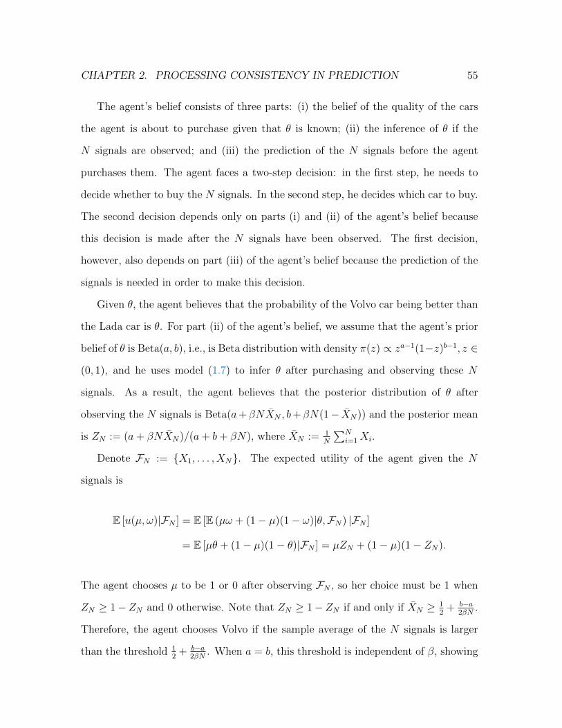
CHAPTER 2. PROCESSING CONSISTENCY IN PREDICTION 55
The agent’s belief consists of three parts: (i) the belief of the quality of the cars
the agent is about to purchase given that θ is known; (ii) the inference of θ if the
N signals are observed; and (iii) the prediction of the N signals before the agent
purchases them. The agent faces a two-step decision: in the first step, he needs to
decide whether to buy the N signals. In the second step, he decides which car to buy.
The second decision depends only on parts (i) and (ii) of the agent’s belief because
this decision is made after the N signals have been observed. The first decision,
however, also depends on part (iii) of the agent’s belief because the prediction of the
signals is needed in order to make this decision.
Given θ, the agent believes that the probability of the Volvo car being better than
the Lada car is θ. For part (ii) of the agent’s belief, we assume that the agent’s prior
belief of θ is Beta(a, b), i.e., is Beta distribution with density π(z) ∝ za−1(1−z)b−1, z ∈
(0, 1), and he uses model (1.7) to infer θ after purchasing and observing these N
signals. As a result, the agent believes that the posterior distribution of θ after
observing the N signals is Beta(a+βNXN , b+βN(1− XN)) and the posterior mean
is ZN := (a+ βNXN)/(a+ b+ βN), where XN := 1N
∑Ni=1 Xi.
Denote FN := X1, . . . , XN. The expected utility of the agent given the N
signals is
E [u(µ, ω)|FN ] = E [E (µω + (1− µ)(1− ω)|θ,FN) |FN ]
= E [µθ + (1− µ)(1− θ)|FN ] = µZN + (1− µ)(1− ZN).
The agent chooses µ to be 1 or 0 after observing FN , so her choice must be 1 when
ZN ≥ 1−ZN and 0 otherwise. Note that ZN ≥ 1−ZN if and only if XN ≥ 12
+ b−a2βN
.
Therefore, the agent chooses Volvo if the sample average of the N signals is larger
than the threshold 12
+ b−a2βN
. When a = b, this threshold is independent of β, showing
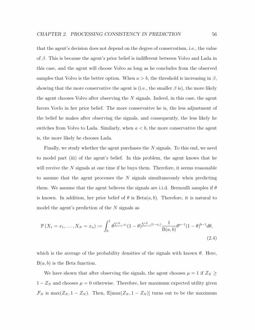
CHAPTER 2. PROCESSING CONSISTENCY IN PREDICTION 56
that the agent’s decision does not depend on the degree of conservatism, i.e., the value
of β. This is because the agent’s prior belief is indifferent between Volvo and Lada in
this case, and the agent will choose Volvo as long as he concludes from the observed
samples that Volvo is the better option. When a > b, the threshold is increasing in β,
showing that the more conservative the agent is (i.e., the smaller β is), the more likely
the agent chooses Volvo after observing the N signals. Indeed, in this case, the agent
favors Vovlo in her prior belief. The more conservative he is, the less adjustment of
the belief he makes after observing the signals, and consequently, the less likely he
switches from Volvo to Lada. Similarly, when a < b, the more conservative the agent
is, the more likely he chooses Lada.
Finally, we study whether the agent purchases the N signals. To this end, we need
to model part (iii) of the agent’s belief. In this problem, the agent knows that he
will receive the N signals at one time if he buys them. Therefore, it seems reasonable
to assume that the agent processes the N signals simultaneously when predicting
them. We assume that the agent believes the signals are i.i.d. Bernoulli samples if θ
is known. In addition, her prior belief of θ is Beta(a, b). Therefore, it is natural to
model the agent’s prediction of the N signals as
P (X1 = x1, . . . , XN = xn) :=
∫ 1
0
θ∑Ni=1 xi(1− θ)
∑Ni=1(1−xi) 1
B(a, b)θa−1(1− θ)b−1dθ,
(2.4)
which is the average of the probability densities of the signals with known θ. Here,
B(a, b) is the Beta function.
We have shown that after observing the signals, the agent chooses µ = 1 if ZN ≥
1−ZN and chooses µ = 0 otherwise. Therefore, her maximum expected utility given
FN is max(ZN , 1 − ZN). Then, E[max(ZN , 1 − ZN)] turns out to be the maximum
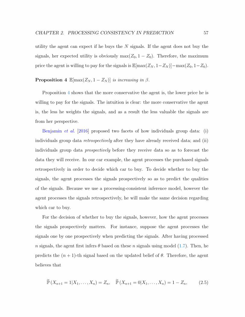
CHAPTER 2. PROCESSING CONSISTENCY IN PREDICTION 57
utility the agent can expect if he buys the N signals. If the agent does not buy the
signals, her expected utility is obviously max(Z0, 1 − Z0). Therefore, the maximum
price the agent is willing to pay for the signals is E[max(ZN , 1−ZN)]−max(Z0, 1−Z0).
Proposition 4 E[max(ZN , 1− ZN)] is increasing in β.
Proposition 4 shows that the more conservative the agent is, the lower price he is
willing to pay for the signals. The intuition is clear: the more conservative the agent
is, the less he weights the signals, and as a result the less valuable the signals are
from her perspective.
Benjamin et al. [2016] proposed two facets of how individuals group data: (i)
individuals group data retrospectively after they have already received data; and (ii)
individuals group data prospectively before they receive data so as to forecast the
data they will receive. In our car example, the agent processes the purchased signals
retrospectively in order to decide which car to buy. To decide whether to buy the
signals, the agent processes the signals prospectively so as to predict the qualities
of the signals. Because we use a processing-consistent inference model, however the
agent processes the signals retrospectively, he will make the same decision regarding
which car to buy.
For the decision of whether to buy the signals, however, how the agent processes
the signals prospectively matters. For instance, suppose the agent processes the
signals one by one prospectively when predicting the signals. After having processed
n signals, the agent first infers θ based on these n signals using model (1.7). Then, he
predicts the (n+ 1)-th signal based on the updated belief of θ. Therefore, the agent
believes that
P (Xn+1 = 1|X1, . . . , Xn) = Zn, P (Xn+1 = 0|X1, . . . , Xn) = 1− Zn, (2.5)
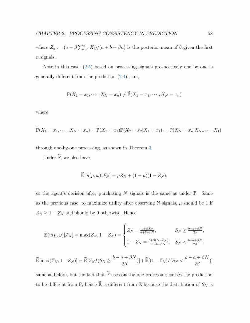
CHAPTER 2. PROCESSING CONSISTENCY IN PREDICTION 58
where Zn := (a + β∑n
i=1Xi)/(a + b + βn) is the posterior mean of θ given the first
n signals.
Note in this case, (2.5) based on processing signals prospectively one by one is
generally different from the prediction (2.4)., i.e.,
P(X1 = x1, · · · , XN = xn) 6= P(X1 = x1, · · · , XN = xn)
where
P(X1 = x1, · · · , XN = xn) = P(X1 = x1)P(X2 = x2|X1 = x1) · · · P(XN = xn|XN−1 · · ·X1)
through one-by-one processing, as shown in Theorem 3.
Under P, we also have
E [u(µ, ω)|FN ] = µZN + (1− µ)(1− ZN),
so the agent’s decision after purchasing N signals is the same as under P. Same
as the previous case, to maximize utility after observing N signals, µ should be 1 if
ZN ≥ 1− ZN and should be 0 otherwise. Hence
E(u(µ, ω)|FN ] = max(ZN , 1− ZN) =
ZN = a+βSN
a+b+βN, SN ≥ b−a+βN
2β,
1− ZN = b+β(N−SN )a+b+βN
, SN < b−a+βN2β
.
E[max(ZN , 1−ZN)] = E[ZNI(SN ≥b− a+ βN
2β)] + E[(1−ZN)I(SN <
b− a+ βN
2β)]
same as before, but the fact that P uses one-by-one processing causes the prediction
to be different from P, hence E is different from E because the distribution of SN is
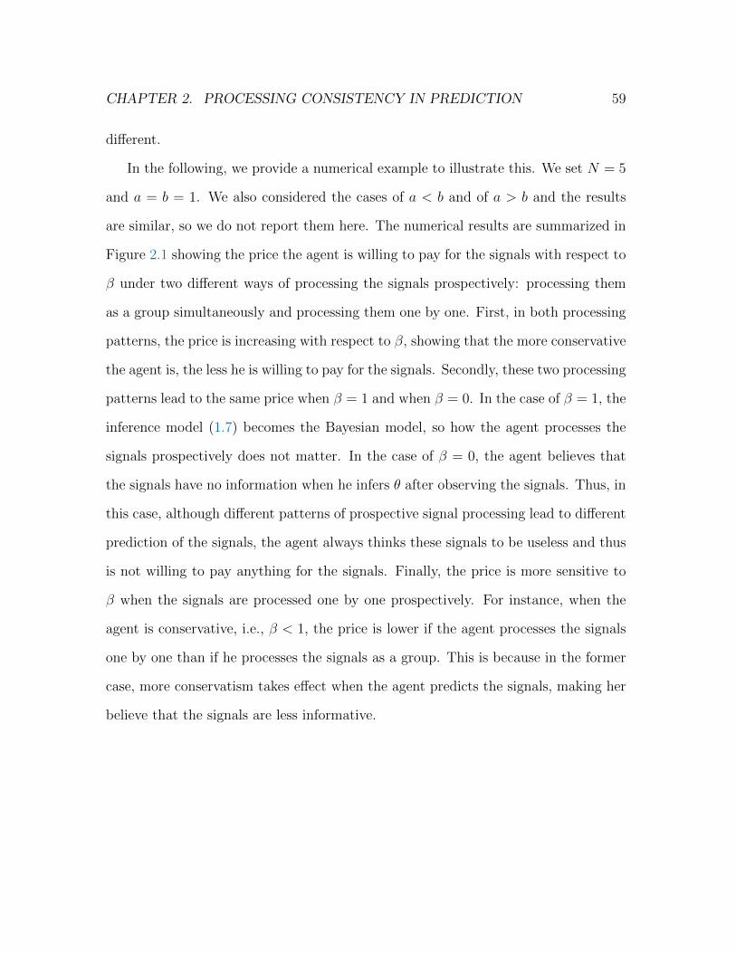
CHAPTER 2. PROCESSING CONSISTENCY IN PREDICTION 59
different.
In the following, we provide a numerical example to illustrate this. We set N = 5
and a = b = 1. We also considered the cases of a < b and of a > b and the results
are similar, so we do not report them here. The numerical results are summarized in
Figure 2.1 showing the price the agent is willing to pay for the signals with respect to
β under two different ways of processing the signals prospectively: processing them
as a group simultaneously and processing them one by one. First, in both processing
patterns, the price is increasing with respect to β, showing that the more conservative
the agent is, the less he is willing to pay for the signals. Secondly, these two processing
patterns lead to the same price when β = 1 and when β = 0. In the case of β = 1, the
inference model (1.7) becomes the Bayesian model, so how the agent processes the
signals prospectively does not matter. In the case of β = 0, the agent believes that
the signals have no information when he infers θ after observing the signals. Thus, in
this case, although different patterns of prospective signal processing lead to different
prediction of the signals, the agent always thinks these signals to be useless and thus
is not willing to pay anything for the signals. Finally, the price is more sensitive to
β when the signals are processed one by one prospectively. For instance, when the
agent is conservative, i.e., β < 1, the price is lower if the agent processes the signals
one by one than if he processes the signals as a group. This is because in the former
case, more conservatism takes effect when the agent predicts the signals, making her
believe that the signals are less informative.
CHAPTER 2. PROCESSING CONSISTENCY IN PREDICTION 60
0 0.5 1 1.5 20
0.05
0.1
0.15
0.2
0.25
0.3
0.35
β
Willin
gnes
s−to−
Pay f
or the
Sign
als
one−by−one processinggroup processing
Figure 2.1: Maximum price the agent is willing to pay for the signals. That is,E[max(ZN , 1−ZN )]−E[max(Z0, 1−Z0)] under two different updating schemes. The num-ber of signals N = 5. The prior distribution of θ is Beta(1,1). The solid line stands for themaximum price the agent is willing to pay for the signals if he processes them as a groupprospectively. The dashed line represents the price when the agent processes the signalsone by one prospectively.
2.4.2 Sequential Purchase of Signals
In the previous setting, the agent decides whether to purchase a given number of
signals at one time, so it is natural for the agent to process the signals he is about
to buy as a group. If the agent can purchase the signals one by one, however, it is
reasonable for him to process the signals one by one.
Consider a variant of the car selection problem in the previous section. We assume
that the agent can purchase signals one by one at unit price c > 0 and decide at any
time whether to stop purchasing additional signals. In this case, it is natural for
the agent to infer the car quality based on the signals he already purchased and
then decide whether to purchase the next signal. Thus, the agent predicts signals
by processing them one by one; i.e., the agent uses one-step transition probability to
update his belief. Consequently, given the n signals the consumer already purchased,
the agent predicts the distribution of the next signal Xn+1 to follow the distribution
CHAPTER 2. PROCESSING CONSISTENCY IN PREDICTION 61
as given in (2.5).
The consumer needs to decide the number of signals τ , which is a stopping time,
he wants to purchase. At each time n, i.e., after already purchasing n signals, the
consumer decides whether to stop purchasing the next signal or not. If he chooses not
to purchase, then based on the n signals, the consumer believes that the probability
that Volvo is better is Zn, and the economic value of this information is max(Zn, 1−
Zn). If the consumer decides to purchase, then with new signal Xn+1, the believes
the probability that Volvo is better is Zn+1, and denote the continuation value as
f(n + 1, Zn+1). On the other hand, the purchase incurs a cost c. Assume that the
consumer is risk neutral. Then, the consumer’s problem is
f(n, Zn) := max
max(Zn, 1− Zn), E[f(n+ 1, Zn+1)|Fn]− c.
Recalling that
Zn+1 =a+ βSn+1
a+ b+ β(n+ 1)
=a+ β(Sn +Xn+1)
a+ b+ β(n+ 1)
=a+ βSna+ b+ βn
a+ b+ βn
a+ b+ β(n+ 1)+
β
a+ b+ β(n+ 1)Xn+1
=(1− wn+1)Zn + wn+1Xn+1,
where wn = βa+b+βn
, and the distribution of Xn+1 given by (2.5), we have
E[f(n+ 1, Zn+1)|Fn] = f(n+ 1, (1− wn+1)Zn + wn+1)Zn
+f(n+ 1, (1− wn+1)Zn)(1− Zn).
CHAPTER 2. PROCESSING CONSISTENCY IN PREDICTION 62
Therefore, the consumer solves the following dynamic programming equation
f(n, Zn) = max
max(Zn, 1− Zn),
f(n+ 1, (1− wn+1)Zn + wn+1)Zn + f(n+ 1, (1− wn+1)Zn)(1− Zn)− c.
(2.6)
Note that when (i) Zn = 0 or Zn = 1 or (ii) n → +∞, an additional signal does
not change the assessment of θ, so the optimal decision in this case must be to stop
purchasing signals and, consequently, we have
f(n, 0) = f(n, 1) = 1, ∀n ≥ 0, (2.7)
limn→+∞
f(n, z) = max(z, 1− z), ∀z ∈ [0, 1]. (2.8)
We solve (2.6)–(2.8) numerically and plot the resulting stopping region, which
consists of two boundaries, z∗,un and z∗,dn , n ≥ 0: the optimal stopping time is
τ ∗ := infn ≥ 0 | Zn ≥ z∗,un or Zn ≤ z∗,dn .
Setting a = b = 1, which implies that the prior belief of θ is the uniform distribution,
we plot the boundaries of the stopping region in Figure 2.2, with the left panel
corresponding to the case in which c = 0.01 and the right panel corresponding to the
case in which c = 0.0001. In each panel, we consider three values of β: 0.5, 1, and 3.
We have the following observations: First, the closer to 0 or 1 the current estimate
of θ is, the less likely the consumer purchases the next signal. This is because the
consumer is more certain about the quality of the cars, so the value of an additional
signal becomes smaller. Second, a higher cost makes the consumer purchase less
signals. Third and most importantly, the smaller β is, the less signals the consumer
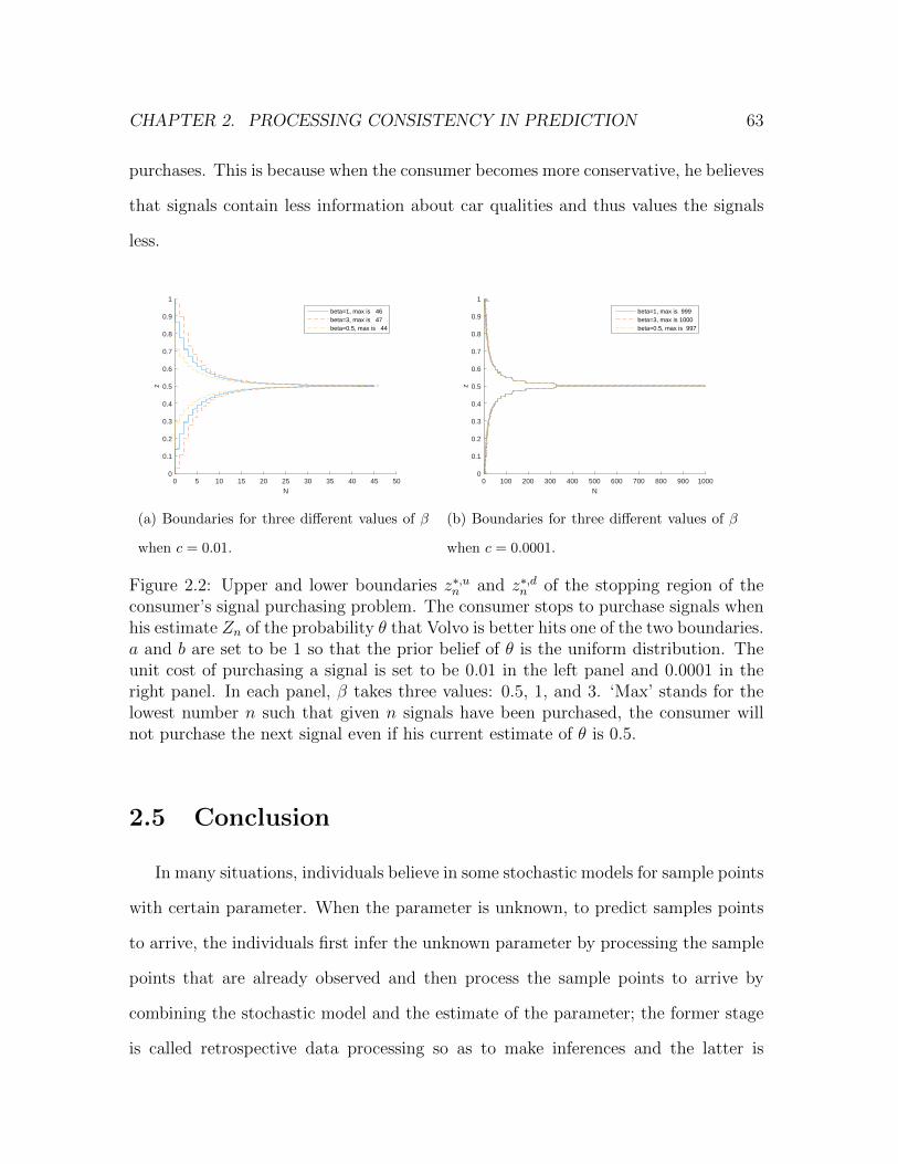
CHAPTER 2. PROCESSING CONSISTENCY IN PREDICTION 63
purchases. This is because when the consumer becomes more conservative, he believes
that signals contain less information about car qualities and thus values the signals
less.
0 5 10 15 20 25 30 35 40 45 50
N
0
0.1
0.2
0.3
0.4
0.5
0.6
0.7
0.8
0.9
1
z
beta=1, max is 46beta=3, max is 47beta=0.5, max is 44
(a) Boundaries for three different values of β
when c = 0.01.
0 100 200 300 400 500 600 700 800 900 1000
N
0
0.1
0.2
0.3
0.4
0.5
0.6
0.7
0.8
0.9
1
z
beta=1, max is 999beta=3, max is 1000beta=0.5, max is 997
(b) Boundaries for three different values of β
when c = 0.0001.
Figure 2.2: Upper and lower boundaries z∗,un and z∗,dn of the stopping region of theconsumer’s signal purchasing problem. The consumer stops to purchase signals whenhis estimate Zn of the probability θ that Volvo is better hits one of the two boundaries.a and b are set to be 1 so that the prior belief of θ is the uniform distribution. Theunit cost of purchasing a signal is set to be 0.01 in the left panel and 0.0001 in theright panel. In each panel, β takes three values: 0.5, 1, and 3. ‘Max’ stands for thelowest number n such that given n signals have been purchased, the consumer willnot purchase the next signal even if his current estimate of θ is 0.5.
2.5 Conclusion
In many situations, individuals believe in some stochastic models for sample points
with certain parameter. When the parameter is unknown, to predict samples points
to arrive, the individuals first infer the unknown parameter by processing the sample
points that are already observed and then process the sample points to arrive by
combining the stochastic model and the estimate of the parameter; the former stage
is called retrospective data processing so as to make inferences and the latter is

CHAPTER 2. PROCESSING CONSISTENCY IN PREDICTION 64
prospective data processing so as to make predictions. In this chapter, assuming
processing consistency in retrospective data processing, we prove that the individuals’
prediction is processing consistent if and only if they use a probabilistic model, i.e.,
uses the Bayes’ rule to make predictions. This result highlights the need of modeling
the means of data processing in a non-Bayesian prediction model.
We then consider a car selection model in which an agent needs to decide whether
to purchase reports that signal the quality of cars in two brands and then decide which
brand to choose. We assume that the agent is conservative when making inferences.
We consider two cases: in the first case, the agent needs to make a one-off purchase
of a certain number of reports; in the second case, the agent can purchase one signal
at one time and decides when to stop purchasing additional signals. Thus, in the
first case, the agent processes reports he is about to purchase as a group and in the
second case, he processes reports one by one. We find that due to conservatism, the
consumer undervalues the signals and thus pay less for the signals or purchase fewer
signals.

Chapter 3
Asset Pricing Applications
3.1 Introduction
In traditional consumption-based asset pricing models, it is assumed that the
distributions of the consumption and dividend streams are known to investors. In
practice, however, such distributions are unknown. For instance, investors may not
know the mean of the growth rate of the dividend of a stock and have to estimate it
from historical data. Thus, statistical inference necessarily plays a role in investors’
portfolio selection and thus affects asset prices. In this chapter, we consider two asset
pricing models in which some model parameters are unknown and thus must be learnt
by the investors from historical data. The investors can be irrational, e.g., subject to
the conservatism bias, when learning the parameters, and we study the impact of the
irrationality on asset prices.
In the first model, we generalize the classical consumption-based asset pricing
model by assuming the mean of the consumption and dividend growth rates to be
unknown. The representative agent in the market must learn the mean from the
historical data, but he may be conservative when making the inference. By assuming
65
CHAPTER 3. ASSET PRICING APPLICATIONS 66
Bernoulli distribution for the dividend growth rates with unknown mean, we solve the
equilibrium asset prices in closed form. We find that when the representative agent
becomes more conservative, the risk-free return and the price-dividend ratio become
less sensitive to the number of good signals in the historical dividend data, and the
risk premium becomes lower.
In the second model, we generalize the asset pricing model in Barberis et al.
[1998] by assuming some of the model parameters to be unknown. More precisely, as
in Barberis et al. [1998], we assume that the true model of the earnings of a stock
is a random walk, but the representative investor in the market wrongly believes in
a regime switching model: one is a trending regime and the other one is a mean-
reverting regime. Unlike Barberis et al. [1998], however, we assume that the model
parameters, i.e., the probability of generating a good earning in these two regimes and
the transition probability from one regime to the other, are unknown. We assume that
the agent uses the model of conservatism to infer the parameters and then evaluate
the stock price by the standard dividend discount model. We compute the stock
price in closed form and study whether this model generates short-term momentum
and long-term reversal as in Barberis et al. [1998] where the model parameters are
known. We find that the more conservative the agent is, the less profound the effect
of short-term momentum and long-term reversal. Also, by comparing with the results
of historical simulation using annual return and net income data of U.S. stocks from
1974 to 2016, we find that investors over-extrapolate the signals in annual income
when making an inference.
CHAPTER 3. ASSET PRICING APPLICATIONS 67
3.2 Consumption-Based Asset Pricing Model
3.2.1 Model
We consider a representative agent whose preferences for discrete-time consump-
tion stream Ct is represented by expected utility; i.e., the preference value at time
t of the consumption stream Cs, s ≥ t is
Vt(C) := Et
[∞∑s=t
ρs−tu(Cs)
],
where Et stands for the expectation conditioning on the information at time t, β is
the discount rate, and the utility function
u(x) :=
x1−γ−1
1−γ , γ 6= 1,
log(x), γ = 1,
for some γ > 0 that represents the degree of relative risk aversion of the agent.
We assume that the agent can trade a stock with price Pt at time t and a risk-free
asset with gross return rate in period t to t+1 to be Rf,t+1. The stock pays a dividend
Dt at time t, so the gross return of holding the stock in period t to t+ 1 is
Rt+1 =Pt+1 +Dt+1
Pt.
We assume that there is no endowment other than the stock dividend in the
market, so the aggregate consumption must be the same as the stock dividend in
equilibrium. We assume that the log dividend growth rates dt+1 := ln (Dt+1/Dt),
t ≥ 0 are i.i.d., but the distribution is unknown to the agent. More precisely, we
assume that dt+1 follows Bernoulli distribution that takes two values y and z with

CHAPTER 3. ASSET PRICING APPLICATIONS 68
probabilities p and 1−p, respectively, and y > z. We assume that y are z are known,
but p is unknown and thus must be learnt by the agent using historical data.
When p is known, the risk-free return and the stock price can be computed by the
Euler equations. More precisely, the risk-free rate in period t to t+1 given parameter
p is
Rf,t+1(p) =
(Et
[ρ
(Ct+1
Ct
)−γ| p
])−1
=(Et[ρe−γdt+1 | p
])−1
=(ρ(e−γyp+ e−γz(1− p)
))−1.
The stock price given p is
Pt(p) = Et
[∞∑j=1
ρj(Ct+jCt
)−γ(Dt+j
Dt
)Dt | p
]
= Dt
∞∑j=1
ρj(E[(Ct+1
Ct)−γ(
Dt+1
Dt
) | p])j
= Dt
∞∑j=1
ρj(E[e(1−γ)dt+1 | p
])j= Dt
ρ[e(1−γ)yp+ e(1−γ)z(1− p))]1− ρ[e(1−γ)yp+ e(1−γ)z(1− p))]
.
When p is unknown, the agent estimates p from the historical data. We assume
that the agent’s prior distribution of p is Beta with parameter (a, b) and the agent
uses the model of conservatism (1.7) to infer p. Consequently, the asset prices are
Rf,t+1 = Et [Rf,t+1(p)] , (3.1)
PtDt
= Et[
ρ[e(1−γ)yp+ e(1−γ)z(1− p))]1− ρ[e(1−γ)yp+ e(1−γ)z(1− p))]
], (3.2)
CHAPTER 3. ASSET PRICING APPLICATIONS 69
where p follows the agent’s posterior distribution of p given the information at time
t. More precisely, according to Table 1.2, the distribution of p is
Beta
(a+ β
t∑i=1
xi, b+ β(t−t∑i=1
xi)
)(3.3)
where
xi :=
1, di = y,
0, di = z.
Note that p can take any values in [0, 1], so for the stock price to be well defined,
we need the make the following assumption on the dividend growth rate:
Assumption 3 ρe(1−γ)y < 1 and ρe(1−γ)z > 1.
3.2.2 Numerical Simulation
Next, we study the impact of conservatism on asset pricing. We set ρ = 0.9, γ = 2,
y = 0.1, and z = −0.1. We assume that the agent’s prior belief of p is Beta(1,1), i.e.,
the uniform distribution, and he observed t = 10 signals, among which∑t
i=1 xi are
good signals.
3.2.2.1 Risk-free Return
We plot the risk-free gross return Rf,t+1 as a function of∑t
i=1 xi, the number of
good signals, for three values of β, 0.5, 1, and 3, in Figure 3.1. We can see that
conservatism (β < 1) leads to a higher risk-free rate when most of the signals are
bad but to a lower risk-free rate when most of the signals are good; in other words,
the risk-free rate is less sensitive with respect to the signals. Intuitively, this is the
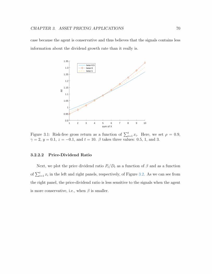
CHAPTER 3. ASSET PRICING APPLICATIONS 70
case because the agent is conservative and thus believes that the signals contains less
information about the dividend growth rate than it really is.
1 2 3 4 5 6 7 8 9 10
sum of X
0.9
0.95
1
1.05
1.1
1.15
1.2
1.25
1.3
1.35R
f
beta=0.5beta=3beta=1
Figure 3.1: Risk-free gross return as a function of∑t
i=1 xi. Here, we set ρ = 0.9,γ = 2, y = 0.1, z = −0.1, and t = 10. β takes three values: 0.5, 1, and 3.
3.2.2.2 Price-Dividend Ratio
Next, we plot the price dividend ratio Pt/Dt as a function of β and as a function
of∑t
i=1 xi in the left and right panels, respectively, of Figure 3.2. As we can see from
the right panel, the price-dividend ratio is less sensitive to the signals when the agent
is more conservative, i.e., when β is smaller.
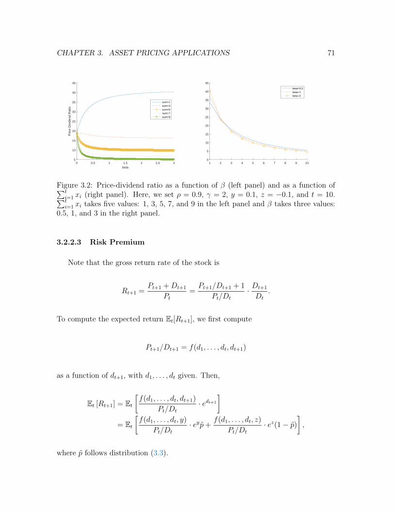
CHAPTER 3. ASSET PRICING APPLICATIONS 71
0 0.5 1 1.5 2 2.5 3
beta
5
10
15
20
25
30
35
40
45
Pric
e D
ivid
end
Rat
io
sum=1sum=3sum=5sum=7sum=9
1 2 3 4 5 6 7 8 9 100
5
10
15
20
25
30
35
40
45
beta=0.5beta=1beta=3
Figure 3.2: Price-dividend ratio as a function of β (left panel) and as a function of∑ti=1 xi (right panel). Here, we set ρ = 0.9, γ = 2, y = 0.1, z = −0.1, and t = 10.∑ti=1 xi takes five values: 1, 3, 5, 7, and 9 in the left panel and β takes three values:
0.5, 1, and 3 in the right panel.
3.2.2.3 Risk Premium
Note that the gross return rate of the stock is
Rt+1 =Pt+1 +Dt+1
Pt=Pt+1/Dt+1 + 1
Pt/Dt
· Dt+1
Dt
.
To compute the expected return Et[Rt+1], we first compute
Pt+1/Dt+1 = f(d1, . . . , dt, dt+1)
as a function of dt+1, with d1, . . . , dt given. Then,
Et [Rt+1] = Et[f(d1, . . . , dt, dt+1)
Pt/Dt
· edt+1
]= Et
[f(d1, . . . , dt, y)
Pt/Dt
· eyp+f(d1, . . . , dt, z)
Pt/Dt
· ez(1− p)],
where p follows distribution (3.3).
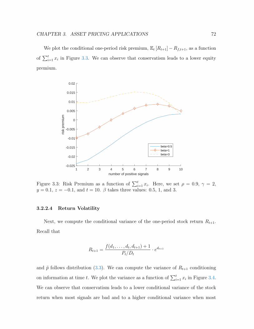
CHAPTER 3. ASSET PRICING APPLICATIONS 72
We plot the conditional one-period risk premium, Et [Rt+1]−Rf,t+1, as a function
of∑t
i=1 xi in Figure 3.3. We can observe that conservatism leads to a lower equity
premium.
1 2 3 4 5 6 7 8 9 10
number of positive signals
-0.025
-0.02
-0.015
-0.01
-0.005
0
0.005
0.01
0.015
0.02
risk
prem
ium
beta=0.5beta=1beta=3
Figure 3.3: Risk Premium as a function of∑t
i=1 xi. Here, we set ρ = 0.9, γ = 2,y = 0.1, z = −0.1, and t = 10. β takes three values: 0.5, 1, and 3.
3.2.2.4 Return Volatility
Next, we compute the conditional variance of the one-period stock return Rt+1.
Recall that
Rt+1 =f(d1, . . . , dt, dt+1) + 1
Pt/Dt
· edt+1
and p follows distribution (3.3). We can compute the variance of Rt+1 conditioning
on information at time t. We plot the variance as a function of∑t
i=1 xi in Figure 3.4.
We can observe that conservatism leads to a lower conditional variance of the stock
return when most signals are bad and to a higher conditional variance when most
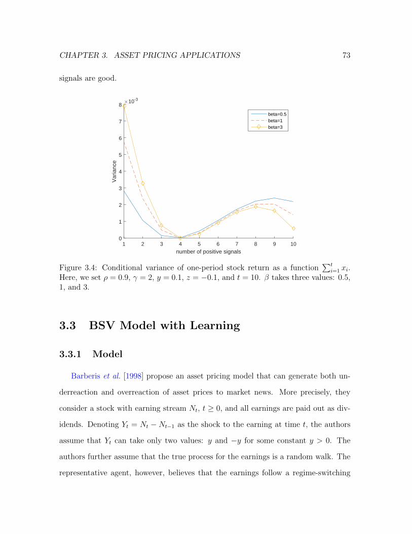
CHAPTER 3. ASSET PRICING APPLICATIONS 73
signals are good.
1 2 3 4 5 6 7 8 9 10
number of positive signals
0
1
2
3
4
5
6
7
8
Var
ianc
e
×10-3
beta=0.5beta=1beta=3
Figure 3.4: Conditional variance of one-period stock return as a function∑t
i=1 xi.Here, we set ρ = 0.9, γ = 2, y = 0.1, z = −0.1, and t = 10. β takes three values: 0.5,1, and 3.
3.3 BSV Model with Learning
3.3.1 Model
Barberis et al. [1998] propose an asset pricing model that can generate both un-
derreaction and overreaction of asset prices to market news. More precisely, they
consider a stock with earning stream Nt, t ≥ 0, and all earnings are paid out as div-
idends. Denoting Yt = Nt − Nt−1 as the shock to the earning at time t, the authors
assume that Yt can take only two values: y and −y for some constant y > 0. The
authors further assume that the true process for the earnings is a random walk. The
representative agent, however, believes that the earnings follow a regime-switching
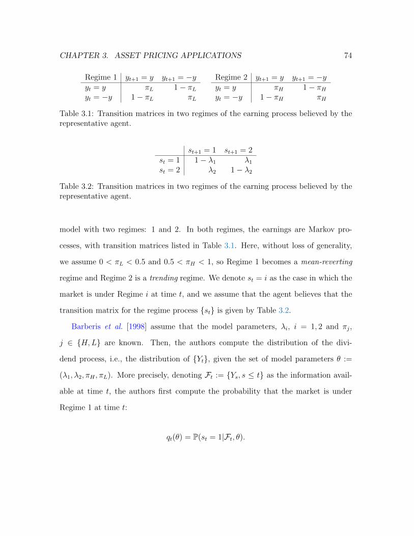
CHAPTER 3. ASSET PRICING APPLICATIONS 74
Regime 1 yt+1 = y yt+1 = −yyt = y πL 1− πLyt = −y 1− πL πL
Regime 2 yt+1 = y yt+1 = −yyt = y πH 1− πHyt = −y 1− πH πH
Table 3.1: Transition matrices in two regimes of the earning process believed by therepresentative agent.
st+1 = 1 st+1 = 2st = 1 1− λ1 λ1
st = 2 λ2 1− λ2
Table 3.2: Transition matrices in two regimes of the earning process believed by therepresentative agent.
model with two regimes: 1 and 2. In both regimes, the earnings are Markov pro-
cesses, with transition matrices listed in Table 3.1. Here, without loss of generality,
we assume 0 < πL < 0.5 and 0.5 < πH < 1, so Regime 1 becomes a mean-reverting
regime and Regime 2 is a trending regime. We denote st = i as the case in which the
market is under Regime i at time t, and we assume that the agent believes that the
transition matrix for the regime process st is given by Table 3.2.
Barberis et al. [1998] assume that the model parameters, λi, i = 1, 2 and πj,
j ∈ H,L are known. Then, the authors compute the distribution of the divi-
dend process, i.e., the distribution of Yt, given the set of model parameters θ :=
(λ1, λ2, πH , πL). More precisely, denoting Ft := Ys, s ≤ t as the information avail-
able at time t, the authors first compute the probability that the market is under
Regime 1 at time t:
qt(θ) = P(st = 1|Ft, θ).
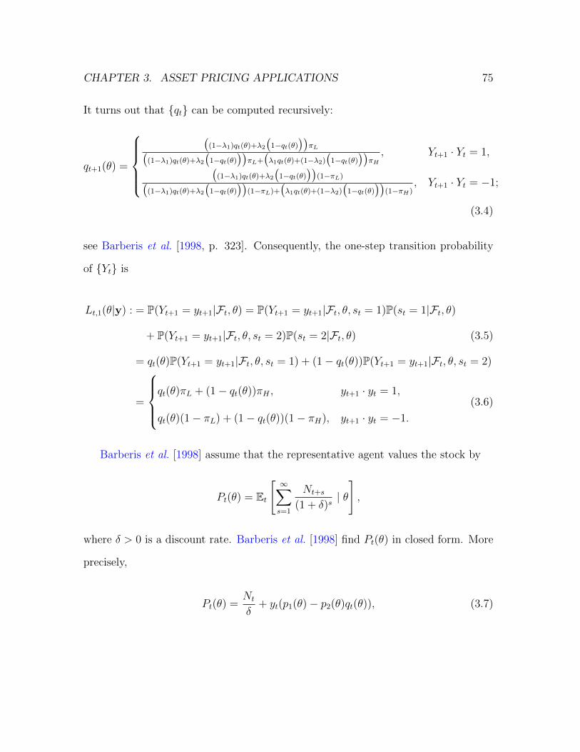
CHAPTER 3. ASSET PRICING APPLICATIONS 75
It turns out that qt can be computed recursively:
qt+1(θ) =
(
(1−λ1)qt(θ)+λ2
(1−qt(θ)
))πL(
(1−λ1)qt(θ)+λ2
(1−qt(θ)
))πL+(λ1qt(θ)+(1−λ2)
(1−qt(θ)
))πH, Yt+1 · Yt = 1,(
(1−λ1)qt(θ)+λ2
(1−qt(θ)
))(1−πL)(
(1−λ1)qt(θ)+λ2
(1−qt(θ)
))(1−πL)+
(λ1qt(θ)+(1−λ2)
(1−qt(θ)
))(1−πH)
, Yt+1 · Yt = −1;
(3.4)
see Barberis et al. [1998, p. 323]. Consequently, the one-step transition probability
of Yt is
Lt,1(θ|y) : = P(Yt+1 = yt+1|Ft, θ) = P(Yt+1 = yt+1|Ft, θ, st = 1)P(st = 1|Ft, θ)
+ P(Yt+1 = yt+1|Ft, θ, st = 2)P(st = 2|Ft, θ) (3.5)
= qt(θ)P(Yt+1 = yt+1|Ft, θ, st = 1) + (1− qt(θ))P(Yt+1 = yt+1|Ft, θ, st = 2)
=
qt(θ)πL + (1− qt(θ))πH , yt+1 · yt = 1,
qt(θ)(1− πL) + (1− qt(θ))(1− πH), yt+1 · yt = −1.
(3.6)
Barberis et al. [1998] assume that the representative agent values the stock by
Pt(θ) = Et
[∞∑s=1
Nt+s
(1 + δ)s| θ
],
where δ > 0 is a discount rate. Barberis et al. [1998] find Pt(θ) in closed form. More
precisely,
Pt(θ) =Nt
δ+ yt(p1(θ)− p2(θ)qt(θ)), (3.7)
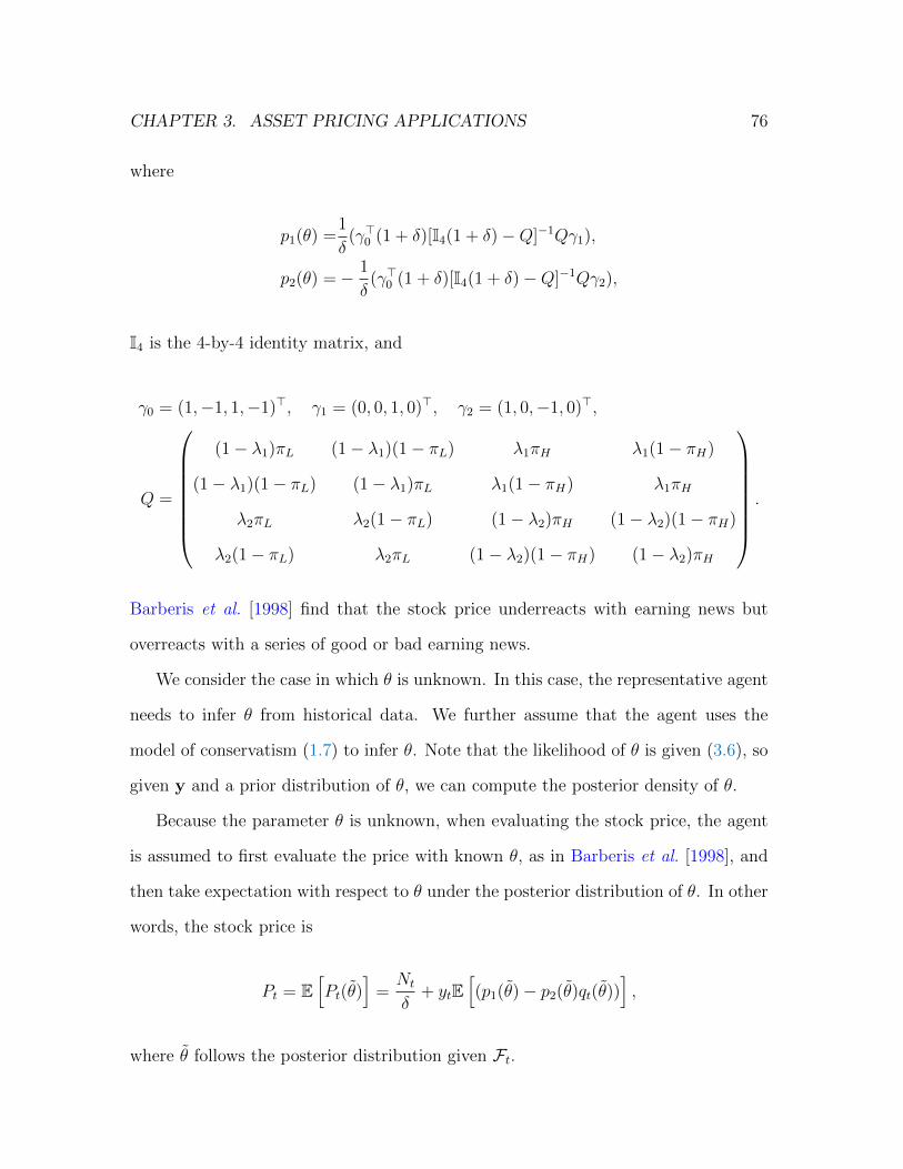
CHAPTER 3. ASSET PRICING APPLICATIONS 76
where
p1(θ) =1
δ(γ>0 (1 + δ)[I4(1 + δ)−Q]−1Qγ1),
p2(θ) =− 1
δ(γ>0 (1 + δ)[I4(1 + δ)−Q]−1Qγ2),
I4 is the 4-by-4 identity matrix, and
γ0 = (1,−1, 1,−1)>, γ1 = (0, 0, 1, 0)>, γ2 = (1, 0,−1, 0)>,
Q =
(1− λ1)πL (1− λ1)(1− πL) λ1πH λ1(1− πH)
(1− λ1)(1− πL) (1− λ1)πL λ1(1− πH) λ1πH
λ2πL λ2(1− πL) (1− λ2)πH (1− λ2)(1− πH)
λ2(1− πL) λ2πL (1− λ2)(1− πH) (1− λ2)πH
.
Barberis et al. [1998] find that the stock price underreacts with earning news but
overreacts with a series of good or bad earning news.
We consider the case in which θ is unknown. In this case, the representative agent
needs to infer θ from historical data. We further assume that the agent uses the
model of conservatism (1.7) to infer θ. Note that the likelihood of θ is given (3.6), so
given y and a prior distribution of θ, we can compute the posterior density of θ.
Because the parameter θ is unknown, when evaluating the stock price, the agent
is assumed to first evaluate the price with known θ, as in Barberis et al. [1998], and
then take expectation with respect to θ under the posterior distribution of θ. In other
words, the stock price is
Pt = E[Pt(θ)
]=Nt
δ+ ytE
[(p1(θ)− p2(θ)qt(θ))
],
where θ follows the posterior distribution given Ft.
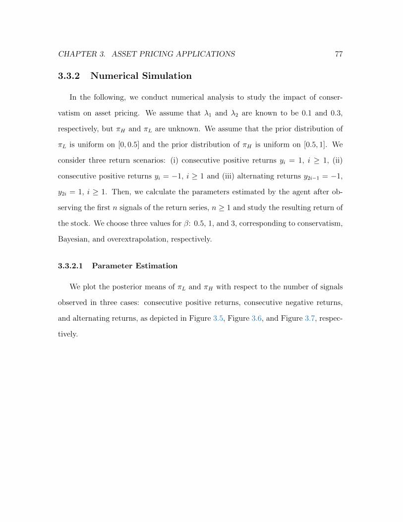
CHAPTER 3. ASSET PRICING APPLICATIONS 77
3.3.2 Numerical Simulation
In the following, we conduct numerical analysis to study the impact of conser-
vatism on asset pricing. We assume that λ1 and λ2 are known to be 0.1 and 0.3,
respectively, but πH and πL are unknown. We assume that the prior distribution of
πL is uniform on [0, 0.5] and the prior distribution of πH is uniform on [0.5, 1]. We
consider three return scenarios: (i) consecutive positive returns yi = 1, i ≥ 1, (ii)
consecutive positive returns yi = −1, i ≥ 1 and (iii) alternating returns y2i−1 = −1,
y2i = 1, i ≥ 1. Then, we calculate the parameters estimated by the agent after ob-
serving the first n signals of the return series, n ≥ 1 and study the resulting return of
the stock. We choose three values for β: 0.5, 1, and 3, corresponding to conservatism,
Bayesian, and overextrapolation, respectively.
3.3.2.1 Parameter Estimation
We plot the posterior means of πL and πH with respect to the number of signals
observed in three cases: consecutive positive returns, consecutive negative returns,
and alternating returns, as depicted in Figure 3.5, Figure 3.6, and Figure 3.7, respec-
tively.
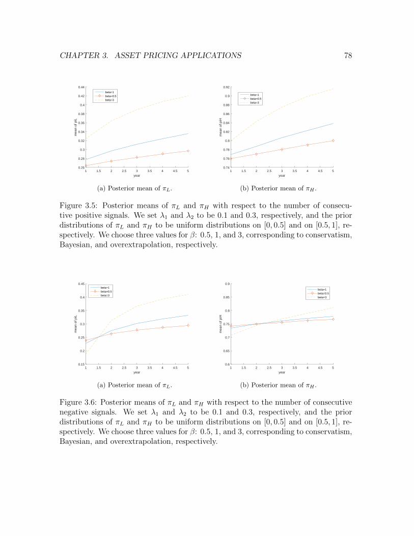
CHAPTER 3. ASSET PRICING APPLICATIONS 78
1 1.5 2 2.5 3 3.5 4 4.5 5
year
0.26
0.28
0.3
0.32
0.34
0.36
0.38
0.4
0.42
0.44
mea
n of
piL
beta=1beta=0.5beta=3
(a) Posterior mean of πL.
1 1.5 2 2.5 3 3.5 4 4.5 5
year
0.74
0.76
0.78
0.8
0.82
0.84
0.86
0.88
0.9
0.92
mea
n of
piH
beta=1beta=0.5beta=3
(b) Posterior mean of πH .
Figure 3.5: Posterior means of πL and πH with respect to the number of consecu-tive positive signals. We set λ1 and λ2 to be 0.1 and 0.3, respectively, and the priordistributions of πL and πH to be uniform distributions on [0, 0.5] and on [0.5, 1], re-spectively. We choose three values for β: 0.5, 1, and 3, corresponding to conservatism,Bayesian, and overextrapolation, respectively.
1 1.5 2 2.5 3 3.5 4 4.5 5
year
0.15
0.2
0.25
0.3
0.35
0.4
0.45
mea
n of
piL
beta=1beta=0.5beta=3
(a) Posterior mean of πL.
1 1.5 2 2.5 3 3.5 4 4.5 5
year
0.6
0.65
0.7
0.75
0.8
0.85
0.9
mea
n of
piH
beta=1beta=0.5beta=3
(b) Posterior mean of πH .
Figure 3.6: Posterior means of πL and πH with respect to the number of consecutivenegative signals. We set λ1 and λ2 to be 0.1 and 0.3, respectively, and the priordistributions of πL and πH to be uniform distributions on [0, 0.5] and on [0.5, 1], re-spectively. We choose three values for β: 0.5, 1, and 3, corresponding to conservatism,Bayesian, and overextrapolation, respectively.
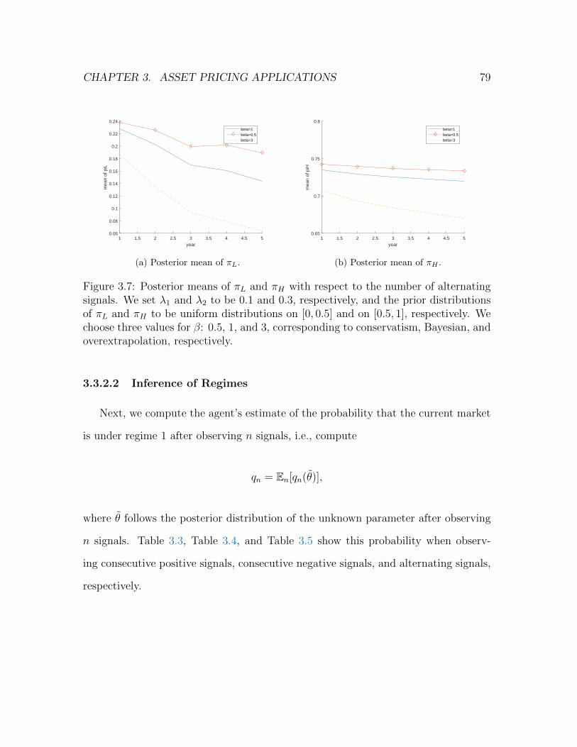
CHAPTER 3. ASSET PRICING APPLICATIONS 79
1 1.5 2 2.5 3 3.5 4 4.5 5
year
0.06
0.08
0.1
0.12
0.14
0.16
0.18
0.2
0.22
0.24
mea
n of
piL
beta=1beta=0.5beta=3
(a) Posterior mean of πL.
1 1.5 2 2.5 3 3.5 4 4.5 5
year
0.65
0.7
0.75
0.8
mea
n of
piH
beta=1beta=0.5beta=3
(b) Posterior mean of πH .
Figure 3.7: Posterior means of πL and πH with respect to the number of alternatingsignals. We set λ1 and λ2 to be 0.1 and 0.3, respectively, and the prior distributionsof πL and πH to be uniform distributions on [0, 0.5] and on [0.5, 1], respectively. Wechoose three values for β: 0.5, 1, and 3, corresponding to conservatism, Bayesian, andoverextrapolation, respectively.
3.3.2.2 Inference of Regimes
Next, we compute the agent’s estimate of the probability that the current market
is under regime 1 after observing n signals, i.e., compute
qn = En[qn(θ)],
where θ follows the posterior distribution of the unknown parameter after observing
n signals. Table 3.3, Table 3.4, and Table 3.5 show this probability when observ-
ing consecutive positive signals, consecutive negative signals, and alternating signals,
respectively.
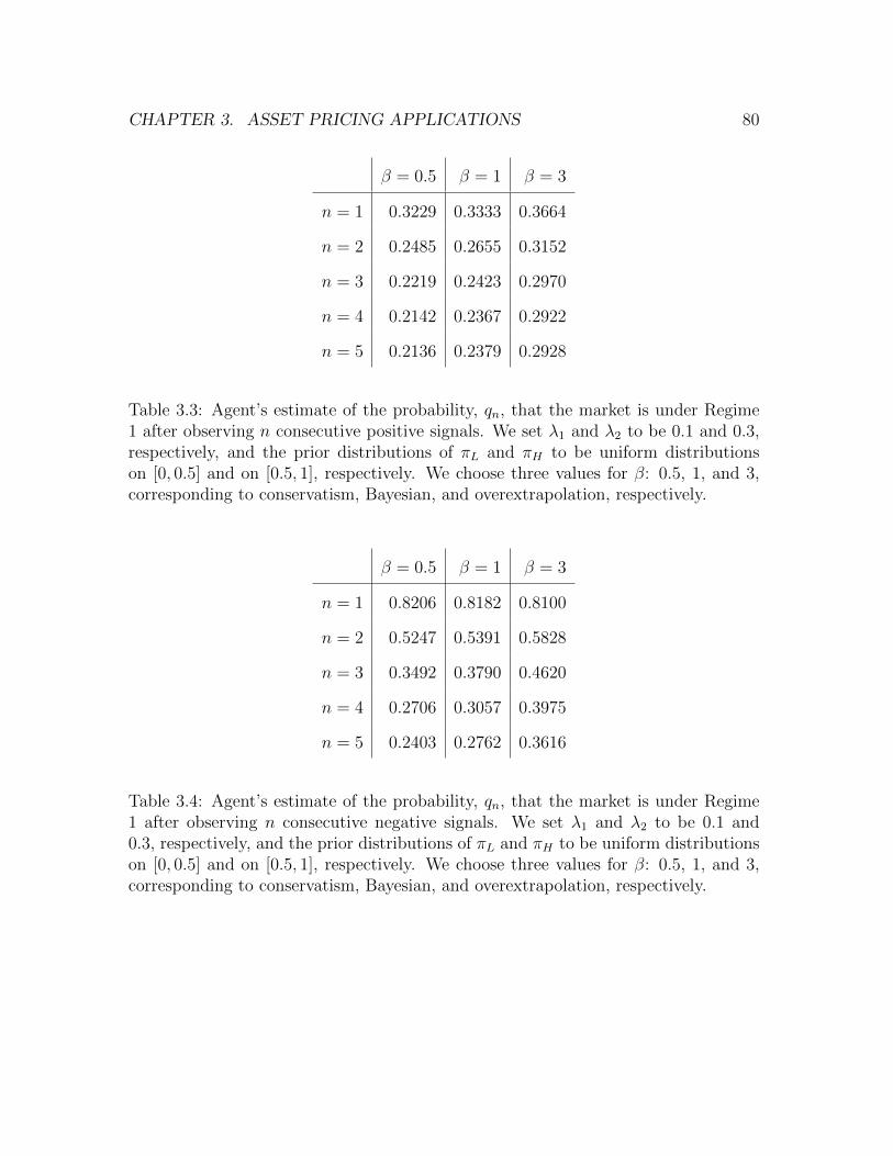
CHAPTER 3. ASSET PRICING APPLICATIONS 80
β = 0.5 β = 1 β = 3
n = 1 0.3229 0.3333 0.3664
n = 2 0.2485 0.2655 0.3152
n = 3 0.2219 0.2423 0.2970
n = 4 0.2142 0.2367 0.2922
n = 5 0.2136 0.2379 0.2928
Table 3.3: Agent’s estimate of the probability, qn, that the market is under Regime1 after observing n consecutive positive signals. We set λ1 and λ2 to be 0.1 and 0.3,respectively, and the prior distributions of πL and πH to be uniform distributionson [0, 0.5] and on [0.5, 1], respectively. We choose three values for β: 0.5, 1, and 3,corresponding to conservatism, Bayesian, and overextrapolation, respectively.
β = 0.5 β = 1 β = 3
n = 1 0.8206 0.8182 0.8100
n = 2 0.5247 0.5391 0.5828
n = 3 0.3492 0.3790 0.4620
n = 4 0.2706 0.3057 0.3975
n = 5 0.2403 0.2762 0.3616
Table 3.4: Agent’s estimate of the probability, qn, that the market is under Regime1 after observing n consecutive negative signals. We set λ1 and λ2 to be 0.1 and0.3, respectively, and the prior distributions of πL and πH to be uniform distributionson [0, 0.5] and on [0.5, 1], respectively. We choose three values for β: 0.5, 1, and 3,corresponding to conservatism, Bayesian, and overextrapolation, respectively.
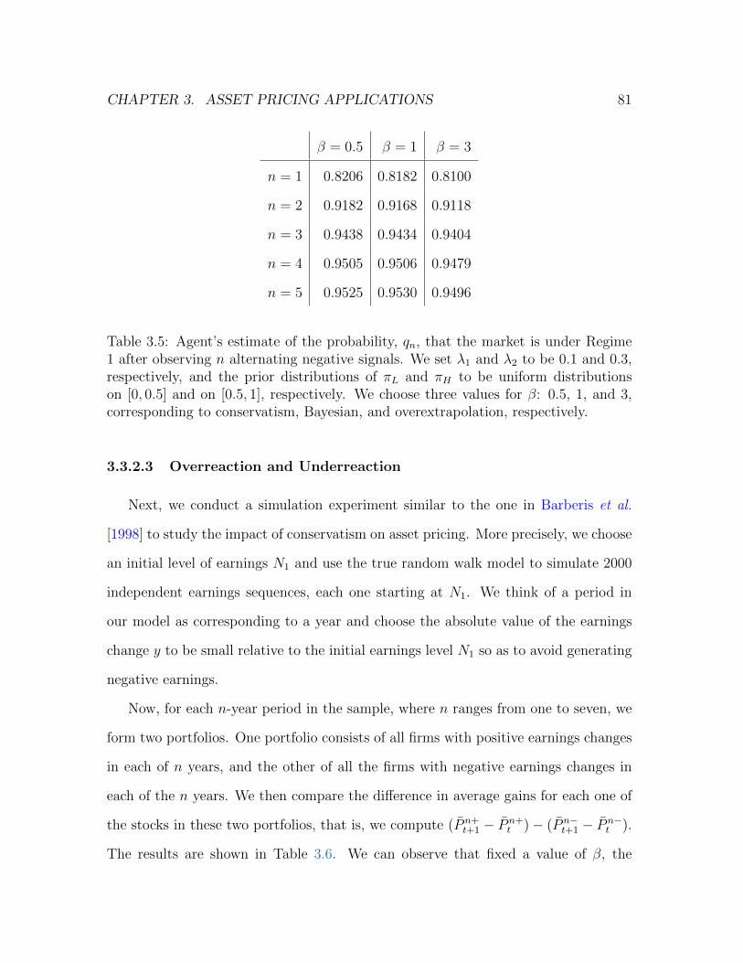
CHAPTER 3. ASSET PRICING APPLICATIONS 81
β = 0.5 β = 1 β = 3
n = 1 0.8206 0.8182 0.8100
n = 2 0.9182 0.9168 0.9118
n = 3 0.9438 0.9434 0.9404
n = 4 0.9505 0.9506 0.9479
n = 5 0.9525 0.9530 0.9496
Table 3.5: Agent’s estimate of the probability, qn, that the market is under Regime1 after observing n alternating negative signals. We set λ1 and λ2 to be 0.1 and 0.3,respectively, and the prior distributions of πL and πH to be uniform distributionson [0, 0.5] and on [0.5, 1], respectively. We choose three values for β: 0.5, 1, and 3,corresponding to conservatism, Bayesian, and overextrapolation, respectively.
3.3.2.3 Overreaction and Underreaction
Next, we conduct a simulation experiment similar to the one in Barberis et al.
[1998] to study the impact of conservatism on asset pricing. More precisely, we choose
an initial level of earnings N1 and use the true random walk model to simulate 2000
independent earnings sequences, each one starting at N1. We think of a period in
our model as corresponding to a year and choose the absolute value of the earnings
change y to be small relative to the initial earnings level N1 so as to avoid generating
negative earnings.
Now, for each n-year period in the sample, where n ranges from one to seven, we
form two portfolios. One portfolio consists of all firms with positive earnings changes
in each of n years, and the other of all the firms with negative earnings changes in
each of the n years. We then compare the difference in average gains for each one of
the stocks in these two portfolios, that is, we compute (P n+t+1 − P n+
t )− (P n−t+1 − P n−
t ).
The results are shown in Table 3.6. We can observe that fixed a value of β, the
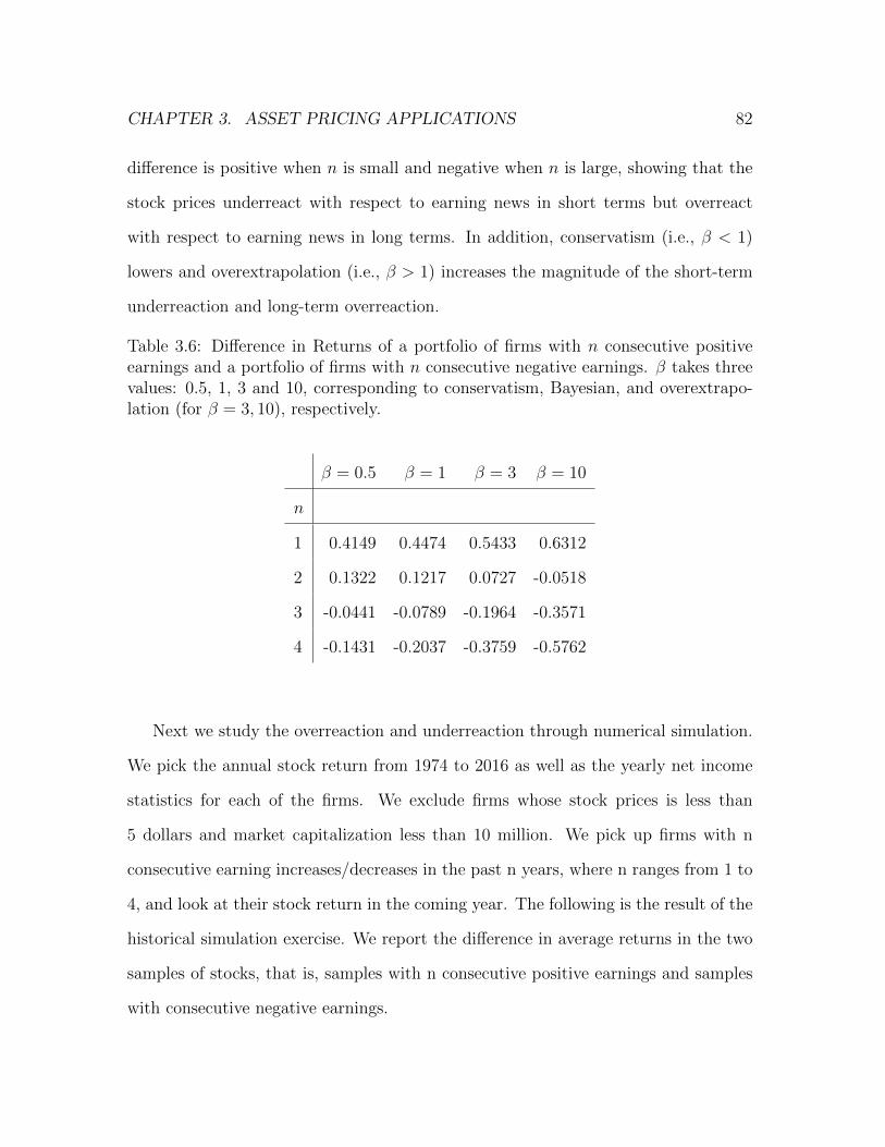
CHAPTER 3. ASSET PRICING APPLICATIONS 82
difference is positive when n is small and negative when n is large, showing that the
stock prices underreact with respect to earning news in short terms but overreact
with respect to earning news in long terms. In addition, conservatism (i.e., β < 1)
lowers and overextrapolation (i.e., β > 1) increases the magnitude of the short-term
underreaction and long-term overreaction.
Table 3.6: Difference in Returns of a portfolio of firms with n consecutive positiveearnings and a portfolio of firms with n consecutive negative earnings. β takes threevalues: 0.5, 1, 3 and 10, corresponding to conservatism, Bayesian, and overextrapo-lation (for β = 3, 10), respectively.
β = 0.5 β = 1 β = 3 β = 10
n
1 0.4149 0.4474 0.5433 0.6312
2 0.1322 0.1217 0.0727 -0.0518
3 -0.0441 -0.0789 -0.1964 -0.3571
4 -0.1431 -0.2037 -0.3759 -0.5762
Next we study the overreaction and underreaction through numerical simulation.
We pick the annual stock return from 1974 to 2016 as well as the yearly net income
statistics for each of the firms. We exclude firms whose stock prices is less than
5 dollars and market capitalization less than 10 million. We pick up firms with n
consecutive earning increases/decreases in the past n years, where n ranges from 1 to
4, and look at their stock return in the coming year. The following is the result of the
historical simulation exercise. We report the difference in average returns in the two
samples of stocks, that is, samples with n consecutive positive earnings and samples
with consecutive negative earnings.
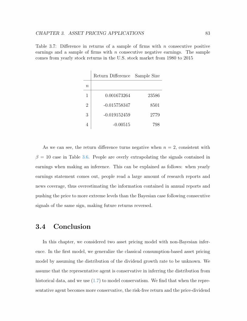
CHAPTER 3. ASSET PRICING APPLICATIONS 83
Table 3.7: Difference in returns of a sample of firms with n consecutive positiveearnings and a sample of firms with n consecutive negative earnings. The samplecomes from yearly stock returns in the U.S. stock market from 1980 to 2015
Return Difference Sample Size
n
1 0.001673264 23586
2 -0.015758347 8501
3 -0.019152459 2779
4 -0.00515 798
As we can see, the return difference turns negative when n = 2, consistent with
β = 10 case in Table 3.6. People are overly extrapolating the signals contained in
earnings when making an inference. This can be explained as follows: when yearly
earnings statement comes out, people read a large amount of research reports and
news coverage, thus overestimating the information contained in annual reports and
pushing the price to more extreme levels than the Bayesian case following consecutive
signals of the same sign, making future returns reversed.
3.4 Conclusion
In this chapter, we considered two asset pricing model with non-Bayesian infer-
ence. In the first model, we generalize the classical consumption-based asset pricing
model by assuming the distribution of the dividend growth rate to be unknown. We
assume that the representative agent is conservative in inferring the distribution from
historical data, and we use (1.7) to model conservatism. We find that when the repre-
sentative agent becomes more conservative, the risk-free return and the price-dividend

CHAPTER 3. ASSET PRICING APPLICATIONS 84
ratio become less sensitive to the number of good signals in the historical dividend
data, and the risk premium becomes lower.
In the second model, we generalize the regime-switching asset pricing model in
Barberis et al. [1998] by assuming some of the model parameters to be unknown.
Again, we assume that the representative agent is conservatism in inferring the pa-
rameters. We find that this model can generate short-term momentum and long-term
reversal, similar to the model in Barberis et al. [1998] where the model parameters
are known. We also find that the more conservative the agent is, the less profound
the effect of short-term momentum and long-term reversal. We finally compare the
numerical result with the data on U.S. stock returns and find that people tend to
overextrapolate the information contained in annual reports when making an infer-
ence.

Bibliography
Maya Bar-Hillel. The base-rate fallacy in probability judgments. Acta Psychologica,
44(3):211–233, 1980.
Maya Bar-Hillel. The base rate fallacy controversy. Decision making under uncer-
tainty, pages 39–61, 1983.
Nicholas Barberis, Andrei Shleifer, and Robert Vishny. A model of investor sentiment.
Journal of Financial Economics, 49(3):307 – 343, 1998.
Lee Roy Beach, James A Wise, and Scott Barclay. Sample proportions and subjective
probability revisions. Organizational Behavior and Human Performance, 5(2):183–
190, 1970.
Lee R Beach. Probability magnitudes and conservative revision of subjective proba-
bilities. Journal of Experimental Psychology, 77(1):57–63, 1968.
Daniel J. Benjamin, Matthew Rabin, and Collin Raymond. A model of non-belief
in the law of large numbers. Journal of the European Economics Association,
14(2):515–544, 2016.
Colin F Camerer. Do biases in probability judgment matter in markets? experimental
evidence. American Economic Review, pages 981–997, 1987.
James O Chinnis Jr and Cameron R Peterson. Inference about a nonstationary
process. Journal of Experimental Psychology, 77(4):620–625, 1968.
Chetan Dave and Katherine W Wolfe. On confirmation bias and deviations from
bayesian updating. Working Paper, 2003.
JH De Swart. Conservatism as a function of bag composition. Acta Psychologica,
36(3):197–206, 1972.
85
BIBLIOGRAPHY 86
JH De Swart. Effects of diagnosticity and prior odds on conservatism in a bookbag-
and-pokerchip situation. Acta Psychologica, 36(1):16–31, 1972.
Michael L Donnell and Wesley M Du Charme. The effect of bayesian feedback on
learning in an odds estimation task. Organizational Behavior and Human Perfor-
mance, 14(3):305–313, 1975.
Ward Edwards. Conservatism in human information processing. In Benjamin Klein-
muntz, editor, Formal representation of human judgment, pages 17–52. Wiley, New
York, 1968.
Larry G Epstein and Michel Le Breton. Dynamically consistent beliefs must be
bayesian. Journal of Economic Theory, 61(1):1–22, 1993.
Larry G Epstein, Jawwad Noor, and Alvaro Sandroni. Non-bayesian updating: a
theoretical framework. Theoretical Economics, 3:193–229, 2008.
Larry G Epstein, Jawwad Noor, and Alvaro Sandroni. Non-Bayesian learning. B.E.
Journal of Theoretical Economics, 10(1):1–20, 2010.
Larry G Epstein. An axiomatic model of non-bayesian updating. Review of Economic
Studies, 73(2):413–436, 2006.
Hans Follmer and Alexander Schied. Stochastic Finance: An Introduction in Discrete
Time. Walter de Gruyter, Berlin, 2nd edition, 2004.
Nicola Gennaioli and Andrei Shleifer. What comes to mind. Quarterly Journal of
Economics, 125(4):1399–1433, 2010.
Jayanta K Ghosh and RV Ramamoorthi. Bayesian nonparametrics. Springer, New
York, 2003.
David M. Grether. Bayes rule as a descriptive model: The representativeness heuristic.
Quarterly Journal of Economics, 95(3):537–557, 1980.
Dale Griffin and Amos Tversky. The weighing of evidence and the determinants of
confidence. Cognitive Psychology, 24(3):411–435, 1992.
Carlo Kraemer and Martin Weber. How do people take into account weight, strength
and quality of segregated vs. aggregated data? experimental evidence. Journal of
Risk and Uncertainty, 29(2):113–142, 2004.
BIBLIOGRAPHY 87
Don Lyon and Paul Slovic. Dominance of accuracy information and neglect of base
rates in probability estimation. Acta Psychologica, 40(4):287–298, 1976.
DF Marks and JK Clarkson. An explanation of conservatism in the bookbag-and-
pokerchips situation. Acta Psychologica, 36(2):145–160, 1972.
Sendhil Mullainathan. Thinking through categories. available at
https://www.chicagobooth.edu/research/workshops/theoryoforg/archive/PDF
/mullainathan.pdf, 2002.
Mark W Nelson, Robert Bloomfield, Jeffrey W Hales, and Robert Libby. The effect of
information strength and weight on behavior in financial markets. Organizational
Behavior and Human Decision Processes, 86(2):168–196, 2001.
Pietro Ortoleva. Modeling the change of paradigm: Non-bayesian reactions to unex-
pected news. American Economic Review, 102(6):2410–2436, 2012.
Cameron R Peterson and Alan J Miller. Sensitivity of subjective probability revision.
Journal of Experimental Psychology, 70(1):117–121, 1965.
Cameron R Peterson and Richard G Swensson. Intuitive statistical inferences about
diffuse hypotheses. Organizational Behavior and Human Performance, 3(1):1–11,
1968.
Cameron R Peterson, Robert J Schneider, and Alan J Miller. Sample size and the
revision of subjective probabilities. Journal of Experimental Psychology, 69(5):522–
527, 1965.
Lawrence D Phillips and Ward Edwards. Conservatism in a simple probability infer-
ence task. Journal of Experimental Psychology, 72(3):346–354, 1966.
Matthew Rabin and Joel L. Schrag. First impressions matter: A model of confirma-
tory bias. Quarterly Journal of Economics, 114(1):37–82, 1999.
Matthew Rabin and Dimitri Vayanos. The gambler’s and hot-hand fallacies: Theory
and applications. Review of Economic Studies, 77(2):730–778, 2010.
Matthew Rabin. Inference by believers in the law of small numbers. Quarterly Journal
of Economics, 117(3):775–816, 2002.
AF Sanders. Choice among bets and revision of opinion. Acta Psychologica, 28:76–83,
1968.

BIBLIOGRAPHY 88
Suzanne Shu and George Wu. Belief bracketing: Can partitioning information change
consumer judgments? Working Paper, Oct. 2003.
Karl Halvor Teigen. Subjective sampling distributions and the additivity of estimates.
Scandinavian Journal of Psychology, 15(1):50–55, 1974.
Amos Tversky and Daniel Kahneman. Judgement under uncertainty: Heuristics and
biases. Science, 185:1124–1131, Sep. 1974.
Abraham Wald. Note on the consistency of the maximum likelihood estimate. Annals
of Mathematical Statistics, 20(4):595–601, 1949.
Gloria Wheeler and Lee Roy Beach. Subjective sampling distributions and conser-
vatism. Organizational Behavior and Human Performance, 3(1):36–46, 1968.
Appendix A
Proofs
A.1 Proofs in Chapter 1
Proof of Proposition 1 The sufficiency is trivial, so we only prove the necessity. We
first prove that there exists Cm > 0 such that gm(z) = Cmg′m(z) for all z in the
effective domain of gm and g′m.
We consider the case in which Θ/Aν 6= ∅ first. In this case, the effective domain
of gm and g′m is [0,+∞). Thus, we only need to show that for any z1 > z2 > 0,
gm(z1)/g′m(z1) = gm(z2)/g′m(z2).
Fix any x ∈ X∞. Because qm,n and q′m,n satisfy Assumption 1, there exists θ0 ∈Θ/Aν and a neighbourhood of θ0, denoted as N , such that (i) N ⊂ Θ/Aν , (ii)
ν(N ) > 0, and (iii) qm,n(θ|x) > 0, q′m,n(θ|x) > 0 for all θ ∈ N . Because ν is σ-finite,
we can find N0 ⊂ N such that 0 < ν(N0) < +∞.
We then choose two different elements in N0 and construct their neighbourhoods
N1 and N2, respectively, such that N1 ∩N2 = ∅, Ni ⊂ N0, and 0 < ν(Ni) < 1/(2z1),
i = 1, 2. Such a construction is possible because ν has no atom on Θ/Aµ; see for
instance Follmer and Schied [2004] Proposition A.27. Define
π(θ) : = z11N1 + z21N2 +1− z1ν(N1)− z2ν(N2)
ν(N0/(N1 ∪N2))1N0/(N1∪N2),
π(θ) : = z11N1∪N2 +1− z1ν(N1 ∪N2)
ν(N0/(N1 ∪N2))1N0/(N1∪N2).
Then, π and π are two probability densities on Θ.
Denote the posterior densities resulted from (1.2) with the prior density π and the
pairs of pseudo-likelihood and distortion (qm,n(θ|x), gm) and (q′m,n(θ|x), g′m) as πm,n
89
APPENDIX A. PROOFS 90
and π′m,n, respectively. Define πm,n and π′m,n similarly. Then, we have πm,n(θ|x) =
π′m,n(θ|x) and πm,n(θ|x) = π′m,n(θ|x) for ν-almost surely θ ∈ Θ. Because ν(N1) >
0, ν(N2) > 0, there exist θ1 ∈ N1 and θ2 ∈ N2 such that πm,n(θi|x) = π′m,n(θi|x) and
πm,n(θi|x) = π′m,n(θi|x), i = 1, 2. In consequence, we have πm,n(θ1|x)/πm,n(θ2|x) =
π′m,n(θ1|x)/π′m,n(θ2|x), which yields
qm,n(θ1|x)gm(π(θ1))
qm,n(θ2|x)gm(π(θ2))=q′m,n(θ1|x)g′m(π(θ1))
q′m,n(θ2|x)g′m(π(θ2))
Because π(θ1) = z1 and π(θ2) = z2, we conclude from the above equation that
qm,n(θ1|x)q′m,n(θ2|x)
qm,n(θ2|x)q′m,n(θ1|x)=gm(z2)g′m(z1)
g′m(z2)gm(z1).
Similarly, we can conclude from πm,n(θi|x) = π′m,n(θi|x), i = 1, 2 that
qm,n(θ1|x)q′m,n(θ2|x)
qm,n(θ2|x)q′m,n(θ1|x)= 1.
As a result, gm(z1)/g′m(z1) = gm(z2)/g′m(z2).
Next, we consider the case in which Aν = Θ. Fix arbitrary θ1, θ2, θ3 ∈ Aµ that are
mutually different. Without loss of generality, we assume that ν(θ1) ≥ ν(θ2) ≥ν(θ3). We first show that gm(z)/g′m(z) is constant for z ∈ (0, 1/ν(θ2, θ3)]. Fix
any z1 < z2 in this interval. Define
π(θ) : = z11θ2 + z21θ3 +1− z1ν(θ2)− z2ν(θ3)
ν(θ1)1θ1,
π(θ) : = z11θ2,θ3 +1− z1ν(θ2, θ3)
ν(θ1)1θ1.
Note that π(·) and π(·) are well-defined probability densities because 0 < z1 < z2 ≤1/ν(θ2, θ3). The same argument as in the case Θ/Aν 6= ∅ yields gm(z1)/g′m(z1) =
gm(z2)/g′m(z2), so gm(z)/g′m(z) is constant for z ∈ (0, 1/ν(θ2, θ3)].Next, for any z2 < 1/ν(θ3), we can always find z1 ∈ (0, 1/ν(θ2, θ3)] such that
both π(·) and π(·) defined above are probability densities. Repeating the previous
argument, we conclude that gm(z2)/g′m(z2) = gm(z1)/g′m(z1), so gm(z)/g′m(z) is con-
stant in (0, 1/ν(θ3)]. Because θi’s are arbitrarily chosen, gm(z)/g′m(z) is constant
in the effective domain of gm and g′m.
Finally, because ν is σ-finite, we can find a probability density π such that π(θ) >
APPENDIX A. PROOFS 91
0, θ ∈ Θ. Because the posterior densities obtained from this prior and the two pairs
(qm,n(θ|x), gm) and (q′m,n(θ|x), g′m) are the same, we conclude, for any x ∈ X∞,
qm,n(θ|x)gm(π(θ))∫Θqm,n(θ|x)gm(π(θ))ν(dθ)
=q′m,n(θ|x)g′m(π(θ))∫
Θq′m,n(θ|x)g′m(π(θ))ν(dθ)
for ν-almost surely θ ∈ Θ, which then holds for any θ ∈ Θ due to the continuity of
qm,n and q′m,n in θ. Because we already showed that gm = Cmg′m for some Cm > 0,
we conclude that
qm,n(θ|x) =Cm∫
Θqm,n(θ|x)gm(π(θ))ν(dθ)∫
Θq′m,n(θ|x)g′m(π(θ))ν(dθ)
q′m,n(θ|x) =: Cm,n(x)q′m,n(θ|x)
for any θ ∈ Θ.
Proof of Theorem 1 We first prove the sufficiency. For any x ∈ X∞ and prior density
π, denote π0,m := IC0,m(x, π), πm,n := ICm,n(x, π0,m), and π0,m+n := IC0,m+n(x, π). On
the one hand,
πm,n(θ|x) =qm,n(θ|x)gm(π0,m(θ|x))∫
Θqm,n(θ|x)gm(π0,m(θ|x))ν(dθ)
=qm,n(θ|x)π0,m(θ|x)∫
Θqm,n(θ|x)π0,m(θ|x)ν(dθ)
=qm,n(θ|x)q0,m(θ|x)g0(π(θ))∫
Θqm,n(θ|x)q0,m(θ|x)g0(π(θ))ν(dθ)
,
where the second equality is the case because gm(z) = Kmz and the third equality
follows from the definition of π0,m. On the other hand,
π0,m+n(θ|x) =q0,m+n(θ|x)g0(π(θ))∫
Θq0,m+n(θ|x)g0(π(θ))ν(dθ)
=qm,n(θ|x)q0,m(θ|x)g0(π(θ))∫
Θqm,n(θ|x)q0,m(θ|x)g0(π(θ))ν(dθ)
,
where the second equality follows from (1.4). Therefore, πm,n(θ|x) = π0,m+n(θ|x) for
all θ ∈ Θ.
Next, we prove the necessity. We first prove condition (i). We consider first
the case in which Θ/Aν 6= ∅. We only need to show that for each fixed m ≥ 1,
gm(z1)/z1 = gm(z2)/z2 for any z1, z2 > 0.
Fix any z1 > z2 > 0 and any x ∈ X∞. Choose θ0 ∈ Θ/Aν such that q0,m+n(θ0|x) >
0, q0,m(θ0|x) > 0, and qm,n(θ0|x) > 0. Choose a neighbourhood N of θ0 such that
N ⊂ Θ/Aν and q0,m+n(θ|x), q0,m(θ|x), qm,n(θ|x) ∈ [ 1C, C],∀θ ∈ N for some C > 0.
Because ν is σ-finite with support Θ, we can findN0 ⊂ N such that 0 < ν(N0) < +∞.
APPENDIX A. PROOFS 92
We first show that, for any bounded probability density p that is null outside N0,
we can find a prior density π such that
p(θ) =q0,m(θ|x)g0(π(θ))∫
Θq0,m(θ|x)g0(π(θ))ν(dθ)
, θ ∈ Θ. (A.1)
To this end, for each δ ≥ 0, define hδ(θ) := g−10
(δp(θ)/q0,m(θ|x)
)1N0(θ), θ ∈ Θ,
where g−10 (y) := +∞ for y ≥ limz→+∞ g0(z). Because 1/C ≤ q0,m(θ|x) ≤ C for all
θ ∈ N0, hz is well-defined. Furthermore, because ν(N0) < +∞ and p is bounded,
the monotone convergence theorem leads to the continuity of λ(δ) :=∫
Θhδ(θ)ν(dθ).
Because g0(0) = 0, we have λ(0) = 0. On the other hand, because ν(N0) > 0, we have
limδ→+∞ λ(δ) = +∞. As a result, there exists δ0 > 0 such that λ(δ0) = 1. Define
π(θ) = hδ0(θ), θ ∈ Θ, then π is a probability density. Furthermore, because gm(0) = 0
and p(θ) ∝ q0,m(θ|x)g0(π(θ)), (A.1) holds.
Now, choose two different elements in N0 and construct their neighbourhoods N1
and N2, respectively, such that N1 ∩ N2 = ∅, Ni ⊂ N0, and 0 < ν(Ni) < 1/(2z1),
i = 1, 2. Such a construction is possible because ν has no atom on Θ/Aµ; see for
instance Follmer and Schied [2004]. Define
p(θ) : = z11N1 + z21N2 +1− z1ν(N1)− z2ν(N2)
ν(N0/(N1 ∪N2))1N0/(N1∪N2).
It is clear that p is a bounded probability density and is null outside N0. Therefore,
we can construct a prior density π such that (A.1) holds. Similarly, for density
p(θ) : = z11N1∪N2 +1− z1ν(N1 ∪N2)
ν(N0/(N1 ∪N2))1N0/(N1∪N2),
we can construct a prior density π such that p and π are related through (A.1).
Next, denote
π0,m := IC0,m(x, π), πm,n := ICm,n(x, π0,m), π0,m+n := IC0,m+n(x, π),
π0,m := IC0,m(x, π), πm,n := ICm,n(x, π0,m), π0,m+n := IC0,m+n(x, π).
Then, π0,m = p and π0,m = p. Due to processing consistency, π0,m+n(θ|x) = πm,n(θ|x)
and π0,m+n(θ|x) = πm,n(θ|x) for ν-almost surely θ ∈ Θ. Because ν(N1) > 0, ν(N2) >
0, there exist θ1 ∈ N1 and θ2 ∈ N2 such that π0,m+n(θi|x) = πm,n(θi|x) and π0,m+n(θi|x) =
πm,n(θi|x), i = 1, 2. Furthermore, because π0,m(θi|x) = p(θi) > 0 and π0,m(θi|x) =
p(θi) > 0, i = 1, 2, and q0,m+n(θ|x) > 0, q0,m(θ|x) > 0, qm,n(θ|x) > 0 for any θ ∈ N0,
APPENDIX A. PROOFS 93
we conclude that π0,m+n(θi|x) = πm,n(θi|x) > 0 and π0,m+n(θi|x) = πm,n(θi|x) > 0,
i = 1, 2. Therefore, we have
π0,m+n(θ1|x)
π0,m+n(θ2|x)=πm,n(θ1|x)
πm,n(θ2|x),
π0,m+n(θ1|x)
π0,m+n(θ2|x)=πm,n(θ1|x)
πm,n(θ2|x)
which leads to
q0,m+n(θ1|x)(p(θ1)/q0,m(θ1|x)
)q0,m+n(θ2|x)
(p(θ2)/q0,m(θ2|x)
) =qm,n(θ1|x)gm(p(θ1))
qm,n(θ2|x)gm(p(θ2)),
q0,m+n(θ1|x)(p(θ1)/q0,m(θ1|x)
)q0,m+n(θ2|x)
(p(θ2)/q0,m(θ2|x)
) =qm,n(θ1|x)gm(p(θ1))
qm,n(θ2|x)gm(p(θ2)).
Because p(θ1) = z1, p(θ2) = z2, and p(θ1) = p(θ2) = z1, we conclude that
q0,m+n(θ1|x)/(q0,m(θ1|x)qm,n(θ1|x)
)q0,m+n(θ2|x)/
(q0,m(θ2|x)qm,n(θ2|x)
) =gm(p(θ1))/p(θ1)
gm(p(θ2))/p(θ2)=gm(z1)/z1
gm(z2)/z2
,
q0,m+n(θ1|x)/(q0,m(θ1|x)qm,n(θ1|x)
)q0,m+n(θ2|x)/
(q0,m(θ2|x)qm,n(θ2|x)
) =gm(p(θ1))/p(θ1)
gm(p(θ2))/p(θ2)=gm(z1)/z1
gm(z1)/z1
= 1.
As a result, gm(z1)/z1 = gm(z2)/z2.
We next consider the case Aν = Θ. Fix arbitrary θ1, θ2, θ3 ∈ Aµ that are mutually
different. Without loss of generality, we assume that ν(θ1) ≥ ν(θ2) ≥ ν(θ3).We first show that gm(z)/z is constant for z ∈ (0, 1/ν(θ2, θ3)]. Fix any z1 < z2 in
this interval. As in the case Θ/Aν 6= ∅, we can show that, for any bounded probability
density p(·) with support within θi|i = 1, 2, 3, we can find a prior density π such
that (A.1) holds. Construct prior densities π and π to generate densities p and p,
respectively, where
p(θ) : = z11θ2 + z21θ3 +1− z1ν(θ2)− z2ν(θ3)
ν(θ1)1θ1,
p(θ) : = z11θ2,θ3 +1− z1ν(θ2, θ3)
ν(θ1)1θ1.
Note that p(·) and p(·) are well-defined probability densities because 0 < z1 < z2 ≤1/ν(θ2, θ3). The same argument as in the case Θ/Aν 6= ∅ yields gm(z1)/z1 =
gm(z2)/z2, so gm(z)/z is constant for z ∈ (0, 1/ν(θ2, θ3)].Next, for any z2 < 1/ν(θ3), we can always find z1 ∈ (0, 1/ν(θ2, θ3)] such
that both p(·) and p(·) defined above are probability densities. Repeating the pre-
APPENDIX A. PROOFS 94
vious argument, we conclude that gm(z2)/z2 = gm(z1)/z1, so gm(z)/z is constant in
(0, 1/ν(θ3)]. Because θi’s are arbitrarily chosen, gm(z)/z is constant in the effective
domain of gm, i.e., condition (i) holds.
Finally, we prove condition (ii). Again, for any x ∈ X∞ and prior density π,
denote π0,m := IC0,m(x, π), πm,n := ICm,n(x, π0,m), and π0,m+n := IC0,m+n(x, π). Because
gm(z) = Kmz, z ≥ 0 for some Km > 0, we have
πm,n(θ|x) =qm,n(θ|x)π0,m(θ|x)∫
Θqm,n(θ|x)π0,m(θ|x)ν(dθ)
=qm,n(θ|x)q0,m(θ|x)g0(π(θ))∫
Θqm,n(θ|x)q0,m(θ|x)g0(π(θ))ν(dθ)
.
On the other hand, we have
π0,m+n(θ|x) =q0,m+n(θ|x)g0(π(θ))∫
Θq0,m+n(θ|x)g0(π(θ))ν(dθ)
.
As a result, for ν-a.e. θ ∈ Θ, we have
qm,n(θ|x)q0,m(θ|x)g0(π(θ))∫Θqm,n(θ|x)q0,m(θ|x)g0(π(θ))ν(dθ)
=q0,m+n(θ|x)g0(π(θ))∫
Θq0,m+n(θ|x)g0(π(θ))ν(dθ)
.
Because ν is σ-finite, we can construct a prior density π such that π(θ) > 0, ∀θ ∈ Θ.
As a result,
q0,m+n(θ|x) = Cm,n(x)qm,n(θ|x)q0,m(θ|x), ν-a.e. θ ∈ Θ
where
Cm,n(x) =
∫Θq0,m+n(θ|x)g0(π(θ))ν(dθ)∫
Θqm,n(θ|x)q0,m(θ|x)g0(π(θ))ν(dθ)
.
Because q0,m, q0,m+n, and qm,n are continuous in θ, we conclude that condition (ii)
holds.
Proof of Proposition 2 Denote T (x, θ) := ln(f(x, θ)/f(x, θ0)) and µ(θ) := Eθ0 [T (Xi, θ)].
Then, because of (1.8) and the dominated convergence theorem, we conclude that µ
is continuous. Furthermore, µ(θ) ≤ 0 for all θ ∈ Θ. In addition, because θ → Πθ is a
one-to-one mapping, µ(θ) = 0 if and only if θ = θ0.
Fix any open neighbourhood U of θ0 and define K := Θ/U . Then, K is closed
and thus compact. For sufficiently small δ, define Vδ := θ|µ(θ) ≥ −δ. Because µ
is continuous, Vδ is closed and thus compact. Define A1 := infθ∈Vδ µ(θ) and A2 :=
APPENDIX A. PROOFS 95
supθ∈K µ(θ). Because µ is continuous, µ(θ0) = 0, and µ(θ) < 0 for any θ 6= θ0, we can
choose δ > 0 such that Vδ ⊂ U and A1 > A2.
For notational simplicity, denote Zn(θ) := 1n
∑ni=1 T (Xi, θ). According to Ghosh
and Ramamoorthi [2003, Theorem 1.3.3], limn→+∞ supθ∈Θ
∣∣Zn(θ)−µ(θ)∣∣ = 0 for Pθ0-
a.s. ω.1 Therefore, for any 0 < ε < (A1 − A2)/2 there exists n0(ω), ω ∈ Ω such that
for Pθ0-a.s. ω, |Zn(θ)− µ(θ)| < ε for any n ≥ n0(ω) and θ ∈ Vδ ∪K. As a result,
∫U
π0,n(θ|X1, X2, . . . )ν(dθ) =
∫U
(∏ni=1 f(Xi, θ)
β)π(θ)ν(dθ)∫
Θ
(∏ni=1 f(Xi, θ)β
)π(θ)ν(dθ)
=
∫U
exp(βnZn(θ)
)π(θ)ν(dθ)∫
Θexp
(βnZn(θ)
)π(θ)ν(dθ)
= 1−
∫K
exp(βnZn(θ)
)π(θ)ν(dθ)∫
Θexp
(βnZn(θ)
)π(θ)ν(dθ)
≥ 1− 1/∫Vδ exp
(βnZn(θ)
)π(θ)ν(dθ)∫
Kexp
(βnZn(θ)
)π(θ)ν(dθ)
+ 1
≥ 1− 1
/(exp (βn(A1 − ε))∫Vδπ(θ)ν(dθ)
exp (βn(A2 + ε))+ 1
),
which goes to 1 as n goes to infinity. Thus, model (1.7) is statistically consistent at
θ0.
Proof of Proposition 3 We use the following notations for the pseudo-likelihood:
q0,1(θ|x1), q0,2(θ|x1, x2), and q1,1(θ|x1, x2) for x1, x2 ∈ X.
If the model of NBLLN is processing consistent, by Theorem 1, there exists
C(x1, x2) > 0 such that
q0,2(θ|x1, x2) = C(x1, x2)q0,1(θ|x1)q1,1(θ|x1, x2), x1, x2 ∈ X, θ ∈ Θ. (A.2)
For each θ, denote Zθ as a random variable living in some probability space and taking
values in Θ with probability density h(·|θ). Then, we have E [Zθ] = θ. Furthermore,
q0,1(θ|x1) = E [f(x1, Zθ)] , q1,1(θ|x1, x2) = E [f(x2, Zθ)] , q0,2(θ|x1, x2) = E [f(x1, Zθ)f(x2, Zθ)] .
1In Ghosh and Ramamoorthi [2003, Theorem 1.3.3], it is assumed that Xi’s take real values.However, this assumption is not needed in the proof of the theorem.
APPENDIX A. PROOFS 96
Set x1 = x2 = 1 and denote C1 := C(1, 1). In this case, we have
q0,1(θ|1) = E[Zθ] = θ, q1,1(θ|1, 1) = E[Zθ] = θ, q0,2(θ|1, 1) = E[Z2θ ].
Then, (A.2) leads to E[Z2θ ] = C1(E[Zθ])
2 = C1θ2. Because of Jensen’s inequality, we
must have C1 > 1.
On the other hand, set x1 = 1, x2 = 0 and denote C2 := C(1, 0). In this case, we
have
q0,1(θ|1) = E[Zθ] = θ, q1,1(θ|1, 0) = E[1− Zθ] = 1− θ, q0,2(θ|1, 0) = E[Zθ(1− Zθ)] = θ − E[Z2θ ].
Then, from (A.2), we have θ − E[Z2θ ] = C2(θ − θ2). Recalling that E[Z2
θ ] = C1θ2, we
conclude
(1− C2)θ − (C1 − C2)θ2 = 0, ∀θ ∈ Θ.
This is true if and only if C1 = C2 = 1, and is contradicted because C1 > 1. Thus,
the pseudo-likelihood in the model of NBLLN does not satisfy the product rule (1.4),
and, as a result, the model of NBLLN is not processing consistent.
Proof of Theorem 2 Part (i): We first prove the sufficiency. For each m ≥ 0, define
˜m,1(θ|x0,m, x) := ϕm(x0,m, x)qm,1(θ|x0,m, x), x0,m ∈ Xm, x ∈ X, θ ∈ Θ (A.3)
and ˜m,n :=
∏m+ni=m+1
˜i−1,1. Because of (1.10), for anym ≥ 0,
∫X
˜m,1(θ|x0,m, x)νX(dx) =
1 for ν-a.e. θ ∈ Θ. Therefore, ˜m,nm≥0,n≥1 is the likelihood of some stochastic model.
Denote the corresponding false-Bayesian model as IBm,nm≥0,n≥1. Because the coher-
ent inference model is assumed to be processing consistent and the false-Bayesian
model is also processing consistent, we only need show that for any x ∈ X∞ and
π ∈ P(Θ), IBn−1,1(x, IB0,n−1(x, π)) = ICn−1,1(x, IC0,n−1(x, π)) for any n ≥ 1. Because g0
is a linear function, we have
IB0,1(x, π)(θ) =˜0,1(θ|x1)π(θ)∫
Θ˜0,1(θ|x1)π(θ)ν(dθ)
=q0,1(θ|x1)π(θ)∫
Θq0,1(θ|x1)π(θ)ν(dθ)
= IC0,1(x, π)(θ)
for ν-a.e. θ ∈ Θ, where the second inequality is the case due to (A.3). The standard
mathematical induction then completes the proof.
Next, we prove the necessity. Suppose there exists a false-Bayesian model IBm,nm≥0,n≥1
with likelihood ˜m,nm≥0,n≥1 such that IBm,n(x, π) = ICm,n(x, π) for any x ∈ X∞,
APPENDIX A. PROOFS 97
π ∈ P(Θ), and m ≥ 0, n ≥ 1. Then, it is clear that ICm,n is processing consistent.
Setting m = 0 and n = 1, we have
˜0,1(θ|x)π(θ)∫
Θ˜0,1(θ|x)π(θ)ν(dθ)
=q0,1(θ|x)g0(π(θ))∫
Θq0,1(θ|x)g0(π(θ))ν(dθ)
, ν-a.e. θ ∈ Θ
for any x ∈ X and π ∈ P(Θ). Using a similar argument to that employed in the proof
of Theorem 1, we can show that g0 is a linear function in its effective domain. As a
result, we have
˜0,1(θ|x)π(θ)∫
Θ˜0,1(θ|x)π(θ)ν(dθ)
=q0,1(θ|x)π(θ)∫
Θq0,1(θ|x)π(θ)ν(dθ)
, ν-a.e. θ ∈ Θ
for any x ∈ X and π ∈ P(Θ). Because ν is σ-finite, we can construct a prior density π
such that π(θ) > 0,∀θ ∈ Θ. Plugging this density into the previous equality, setting
ϕ0(x) :=
∫Θ
˜0,1(θ|x)π(θ)ν(dθ)∫
Θq0,1(θ|x)π(θ)ν(dθ)
, x ∈ X,
and noting that∫X
˜0,1(θ|x)νX(dx) = 1 for any θ ∈ Θ, we immediately conclude that
(1.10) holds for m = 0.
Finally, due to processing consistency, we have
ICn,1(x, IC0,n(x, π)) = IC0,n+1(x, π) = IB0,n+1(x, π) = IBn,1(x, IB0,n(x, π)).
Furthermore, if IC0,n(x, π)(θ) and IB0,n(x, π)(θ) are positive for ν-a.e. θ ∈ Θ, so are
ICn,1(x, IC0,n(x, π))(θ) and IBn,1(x, IB0,n(x, π))(θ). Then, the standard mathematical in-
duction shows that (1.10) holds for any m ≥ 0.
Part (ii): We first prove the necessity. Suppose for any π ∈ P(Θ) there exist a false-
Bayesian model IBm,nm≥0,n≥1 with likelihood ˜m,nm≥0,n≥1 and a false prior density
π such that IBm,n(x, π) = ICm,n(x, π) for any x ∈ X∞ and m ≥ 0, n ≥ 1. Then, it is
clear that ICm,n is processing consistent.
Choose any π ∈ P(Θ) such that π(θ) > 0 for ν-a.e. θ ∈ Θ. By assumption,
IB0,1(x, π) = IC0,1(x, π). Furthermore, we have IC0,1(x, π)(θ) > 0, ν-a.e. θ ∈ Θ. Because
for any m ≥ 1
ICm,1(x, IC0,m(x, π)) = IC0,m+1(x, π) = IB0,m+1(x, π) = IBm,1(x, IB0,m(x, π))
holds for any x ∈ X∞, following the same proof as for part (i) of this theorem, we
APPENDIX A. PROOFS 98
conclude (1.10) holds for any m ≥ 1.
Next, we prove the sufficiency. Fix any π ∈ P(Θ). Because νX is σ-finite
and 0 <∫
Θq0,1(θ|x)g0(π(θ))ν(dθ) < +∞ for each x ∈ X, we can find a count-
able partition An, n ≥ 1 of X and a sequence of positive numbers an, n ≥ 1 such
that∫
Θq0,1(θ|x)g0(π(θ))ν(dθ) ≤ an, x ∈ An and νX(An) ≤ an, n ≥ 1. Define
h0(x) :=∑∞
n=11
2na2n1An(x), x ∈ X. Then,∫
X
∫Θ
h0(x)q0,1(θ|x)g0(π(θ))ν(dθ)νX(dx)
=
∫Xh0(x)
∫Θ
q0,1(θ|x)g0(π(θ))ν(dθ)νX(dx)
=∞∑n=1
∫An
h0(x)
∫Θ
q0,1(θ|x)g0(π(θ))ν(dθ)νX(dx)
≤∞∑n=1
1
2na2n
anν(An) ≤ 1 < +∞.
Consequently, g0(π(θ))∫X h0(x)q0,1(θ|x)νX(dx) < +∞ for ν-a.e. θ ∈ Θ. Denote Θ0 :=
θ ∈ Θ|π(θ) = 0. For any θ ∈ Θ\Θ0, g0(π(θ)) > 0, so∫X h0(x)q0,1(θ|x)νX(dx) <
+∞. As a result, for any θ ∈ Θ\Θ0, we can define
π(θ) :=g0(π(θ))
∫X h0(x)q0,1(θ|x)νX(dx)∫
X
∫Θh0(x)q0,1(θ|x)g0(π(θ))ν(dθ)νX(dx)
, ˜0,1(θ|x) :=
h0(x)q0,1(θ|x)∫X h0(x)q0,1(θ|x)νX(dx)
.
For θ ∈ Θ0, define π(θ) = 0 and ˜0,1(θ|x) = p(x), x ∈ X for an arbitrarily chosen p
such that p(x) ≥ 0, x ∈ X and∫X p(x)νX(dx) = 1.
Now, define ˜m,1 for m ≥ 1 as in (A.3) and define ˜
m,n :=∏m+n
i=m+1˜i−1,1 for m ≥ 0
and n ≥ 1. One can verify that∫X
˜m,1(θ|x0,m, x)νX(dx) = 1 for any x0,m ∈ Xm,
θ ∈ Θ, and m ≥ 0, so ˜m,n is the likelihood of a false model. Denote by IBm,n the
false-Bayesian model associated with this false likelihood. Then, we have
IB0,1(x, π)(θ) =˜0,1(θ|x1)π(θ)∫
Θ˜0,1(θ|x1)π(θ)ν(dθ)
=h0(x1)q0,1(θ|x1)g0(π(θ))∫
Θh0(x1)q0,1(θ|x1)g0(π(θ))ν(dθ)
=q0,1(θ|x1)g0(π(θ))∫
Θq0,1(θ|x1)g0(π(θ))ν(dθ)
= IC0,1(x, π)(θ), ν-a.e. θ ∈ Θ.
Finally, using the same argument as in the proof of part (i) of the theorem, we can
APPENDIX A. PROOFS 99
conclude that for any m ≥ 1
IC0,m+1(x, π) = ICm,1(x, IC0,m(x, π)) = IBm,1(x, IB0,m(x, π)) = IB0,m+1(x, π).
A.2 Proofs in Chapter 2
Proof of Theorem 3 We first prove the sufficiency; i.e., suppose (2.3) holds and we
prove that (2.2) holds. To this end, we only need to prove that (2.2) holds for any
m ≥ 0 and n1 = n2 = 1. In the following proof, when m = 0, πm stands for the
distorted prior as defined in (1.5).
Because both `m,n and qm,n satisfy the product rule and (2.3) holds, there
exists Cm(x) > 0 that is independent of θ such that
qm,1(θ|x) = Cm(x)`m,1(θ|x), θ ∈ Θ.
Consequently,
µm,1(x)µm+1,1(x) =
∫Θ
`m,1(θ|x)πm(θ|x)ν(dθ)
∫Θ
`m+1,1(θ|x)πm,1(θ|x)ν(dθ)
=
∫Θ
`m,1(θ|x)πm(θ|x)ν(dθ)
∫Θ
`m+1,1(θ|x)qm,1(θ|x)πm(θ|x)∫
Θqm,1(θ|x)πm(θ|x)ν(dθ)
ν(dθ)
=
∫Θ
`m,1(θ|x)πm(θ|x)ν(dθ)
∫Θ
`m+1,1(θ|x)`m,1(θ|x)πm(θ|x)∫
Θ`m,1(θ|x)πm(θ|x)ν(dθ)
ν(dθ)
=
∫Θ
`m+1,1(θ|x)`m,1(θ|x)πm(θ|x)ν(dθ)
=
∫Θ
`m,2(θ|x)πm(θ|x)ν(dθ)
= µm,2(x).
Next, we prove the necessity. We first consider the case in which Aν = Θ. In
this case, consider any θ1, θ2 ∈ Θ. Fixing m ≥ 0 and x0,m ∈ Xm, for any y ≥ 0 and
z ≥ 0 such that ν(θ1)y + ν(θ2)z = 1, we can find a prior density πm such that
APPENDIX A. PROOFS 100
πm(θ1|x) = y and πm(θ2|x) = z; see the proof of Theorem 1. Then,
πm+1(θ1|x) =qm,1(θ1|x)y
qm,1(θ1|x)ν(θ1)y + qm,1(θ2|x)ν(θ2)z,
πm+1(θ2|x) =qm,1(θ2|x)z
qm,1(θ1|x)ν(θ1)y + qm,1(θ2|x)ν(θ2)z.
Consequently, because (2.2) holds for n1 = n2 = 1, we have
`m,2(θ1|x)ν(θ1)y + `m,2(θ2|x)ν(θ2)z=(`m,1(θ1|x)ν(θ1)y + `m,1(θ2|x)ν(θ2)z
)× `m+1,1(θ1|x)qm,1(θ1|x)ν(θ1)y + `m+1,1(θ2|x)qm,1(θ2|x)ν(θ2)z
qm,1(θ1|x)ν(θ1)y + qm,1(θ2|x)ν(θ2)z,
which, together with ν(θ1)y + ν(θ2)z = 1, implies
[`m,2(θ1|x)ν(θ1)y + `m,2(θ2|x)(1− ν(θ1)y)][qm,1(θ1|x)ν(θ1)y + qm,1(θ2|x)(1− ν(θ1)y)]
=[`m,1(θ1|x)ν(θ1)y + `m,1(θ2|x)(1− ν(θ1)y)]×[`m+1,1(θ1|x)qm,1(θ1|x)ν(θ1)y + `m+1,1(θ2|x)qm,1(θ2|x)(1− ν(θ1)y)].
Note that the above equation holds for any y such that ν(θ1)y ∈ [0, 1], so each of
the y2 term, y term, and constant term in the above equation must be zero. This
implies
qm,1(θ1|x)`m,2(θ2|x) + qm,1(θ2|x)`m,2(θ1|x)
=`m,1(θ2|x)qm,1(θ1|x)`m+1,1(θ1|x) + `m,1(θ1|x)qm,1(θ2|x)`m+1,1(θ2|x). (A.4)
Because `m,2(θ|x) = `m,1(θ|x)`m+1,1(θ|x) for any θ ∈ Θ, (A.4) yields
`m,1(θ1|x)`m+1,1(θ1|x)qm,1(θ2|x) + qm,1(θ1|x)`m,1(θ2|x)`m+1,1(θ2|x)
=`m,1(θ1|x)`m+1,1(θ2|x)qm,1(θ2|x) + `m,1(θ2|x)`m+1,1(θ1|x)qm,1(θ1|x). (A.5)
Now, define LRm+1,1(θ1, θ2|x) = `m+1,1(θ1|x)
`m+1,1(θ2|x), QRm,1(θ1, θ2|x) = qm,1(θ1|x)
qm,1(θ2|x), LRm,1(θ1, θ2|x) =
`m,1(θ1|x)
`m,1(θ2|x). Dividing both sides of (A.5) by `m+1,1(θ2|x)`m,1(θ2|x)qm,1(θ2|x), we obtain
LRm,1(θ1, θ2|x)LRm+1,1(θ1, θ2|x) +QRm,1(θ1, θ2|x)
= LRm,1(θ1, θ2|x) + LRm+1,1(θ1, θ2|x)QRm,1(θ1, θ2|x),
APPENDIX A. PROOFS 101
which implies
(LRm+1,1(θ1, θ2|x)− 1)(LRm,1(θ1, θ2|x)−QRm,1(θ1, θ2|x)) = 0. (A.6)
We claim that (A.6) implies that LRm,1(θ1, θ2|x) = QRm,1(θ1, θ2|x). Suppose for the
sake of contradiction that LRm,1(θ1, θ2|x) 6= QRm,1(θ1, θ2|x). Then, we must have
LRm+1,1(θ1, θ2|x) = 1. Note that LRm,1(θ1, θ2|x) and QRm,1(θ1, θ2|x) depend on xm+1
only, but LRm+1,1(θ1, θ2|x) depends on xm+1,1. Because given xm+1, LRm+1,1(θ1, θ2|x)
cannot be constant with respect to xm+1,1, we conclude that LRm+1,1(θ1, θ2|x) cannot
be equal to 1. Consequently, we have LRm,1(θ1, θ2|x) = QRm,1(θ1, θ2|x).
We have shown that for any θ1, θ2 ∈ Θ = Aν , LRm,1(θ1, θ2|x) = QRm,1(θ1, θ2|x).
It is straightforward to see that this is equivalent to the existence of Cm,1(x) > 0 such
that
qm,1(θ|x) = Cm,1(x)`0,1(θ|x), , θ ∈ Θ.
Because both qm,n and `m,n satisfy the product rule, we conclude (2.3) holds for
any m.
Next, we consider the general case. Again, we only need to prove that for m ≥ 0,
any x ∈ X∞, and any θ1, θ2 ∈ Θ, LRm,1(θ1, θ2|x) = QRm,1(θ1, θ2|x).
Given m ≥ 0, for the sake of contradiction, suppose that there exists x and
θ1, θ2 ∈ Θ such that LRm,1(θ1, θ2|x) 6= QRm,1(θ1, θ2|x). We can find x such that (i)
x0,m+1 = x0,m+1, which implies that `m,1(θ|x) = `m,1(θ|x) and qm,1(θ|x) = qm,1(θ|x)
for any θ ∈ Θ, and (ii) LRm+1,1(θ1, θ2|x) 6= LRm+1,1(θ1, θ2|x).
If θi ∈ Aν , we define Ni := θi. If θi /∈ Aν , for any ε > 0, with Assumption
2 in place, we can find a neighbourhood Ni of θi such that (i) ν(Ni) ∈ (0, ε), (ii)
N1∩N2 = ∅, (iii) |`m,1(θ|x)−`m,1(θi|x)| < ε, |qm,1(θ|x)−qm,1(θi|x)| < ε, |`m+1,1(θ|x)−`m+1,1(θi|x)| < ε, |`m+1,1(θ|x)− `m+1,1(θi|x)| < ε, ∀θ ∈ Ni.
Now, for any y ≥ 0 and z ≥ 0 such that ν(N1)y+ ν(N2)z = 1, we can find a prior
density π0 such that πm(θ|x) = y, θ ∈ N1 and πm(θ|x) = z, θ ∈ N2; see the proof of
Theorem 1. Then,
πm+1(θ|x) =qm,1(θ|x)y1N1 + qm,1(θ|x)z1N2
y∫N1qm,1(θ|x)ν(dθ) + z
∫N2qm,1(θ|x)ν(dθ)
.
APPENDIX A. PROOFS 102
Consequently, because (2.2) holds for n1 = n2 = 1, we have
y
∫N1
`m,2(θ|x)ν(dθ) + z
∫N2
`m,2(θ|x)ν(dθ) =y∫N1`m,1(θ|x)ν(dθ) + z
∫N2`m,1(θ|x)ν(dθ)
y∫N1qm,1(θ|x)ν(dθ) + z
∫N2qm,1(θ|x)ν(dθ)
×(y
∫N1
`m+1,1(θ|x)qm,1(θ|x)ν(dθ) + z
∫N2
`m+1,1(θ|x)qm,1(θ|x)ν(dθ)
),
which, together with ν(N1)y + ν(N2)z = 1, implies
(
∫N1
`m,2(θ|x)ν(dθ)
∫N1
qm,1(θ|x)ν(dθ)−∫N1
`m,1(θ|x)ν(dθ)
∫N1
`m+1,1(θ|x)qm,1(θ|x)ν(dθ))y2
+ (
∫N2
`m,2(θ|x)ν(dθ)
∫N1
qm,1(θ|x)ν(dθ) +
∫N1
`m,2(θ|x)ν(dθ)
∫N2
qm,1(θ|x)ν(dθ)
−∫N1
`m,1(θ|x)ν(dθ)
∫N2
`m+1,1(θ|x)qm,1(θ|x)ν(dθ)
−∫N1
`m+1,1(θ|x)qm,1(θ|x)ν(dθ)
∫N2
`m,1(θ|x)ν(dθ))1− yν(N1)
ν(N2)y
+
(∫N2
qm,1(θ|x)ν(dθ)
∫N2
`m,2(θ|x)ν(dθ)−∫N2
`m,1(θ|x)ν(dθ)
∫N2
`m+1,1(θ|x)qm,1(θ|x)ν(dθ)
)× (1− yν(N1))2
ν(N2)2= 0
The above equation holds for any y > 0 such that ν(N1)y ≤ 1, so each of the y2, y,
APPENDIX A. PROOFS 103
and constant terms should be zero. Thus, we have the following three equations:∫N1
`m,2(θ|x)ν(dθ)
∫N1
qm,1(θ|x)ν(dθ)−∫N1
`m,1(θ|x)ν(dθ)
∫N1
`m+1,1(θ|x)qm,1(θ|x)ν(dθ)
− ν(N1)
ν(N2)
[ ∫N2
`m,2(θ|x)ν(dθ)
∫N1
qm,1(θ|x)ν(dθ) +
∫N1
`m,2(θ|x)ν(dθ)
∫N2
qm,1(θ|x)ν(dθ)
−∫N1
`m,1(θ|x)ν(dθ)
∫N2
`m+1,1(θ|x)qm,1(θ|x)ν(dθ)
−∫N2
`m,1(θ|x)ν(dθ)
∫N1
`m+1,1(θ|x)qm,1(θ|x)ν(dθ)
]+
(ν(N1)
ν(N2)
)2 [ ∫N2
qm,1(θ|x)ν(dθ)
∫N2
`m,2(θ|x)ν(dθ)
−∫N2
`m,1(θ|x)ν(dθ)
∫N2
`m+1,1(θ|x)qm,1(θ|x)ν(dθ)
]= 0, (A.7)
− 2ν(N1)
ν(N2)2
[ ∫N2
qm,1(θ|x)ν(dθ)
∫N2
`m,2(θ|x)ν(dθ)
−∫N2
`m,1(θ|x)ν(dθ)
∫N2
`m+1,1(θ|x)qm,1(θ|x)ν(dθ)
]+
1
ν(N2)
[ ∫N2
`m,2(θ|x)ν(dθ)
∫N1
qm,1(θ|x)ν(dθ) +
∫N1
`m,2(θ|x)ν(dθ)
∫N2
qm,1(θ|x)ν(dθ)
−∫N1
`m,1(θ|x)ν(dθ)
∫N2
`m+1,1(θ|x)qm,1(θ|x)ν(dθ)
−∫N2
`m,1(θ|x)ν(dθ)
∫N1
`m+1,1(θ|x)qm,1(θ|x)ν(dθ)
]= 0, (A.8)
1
ν(N2)2
[ ∫N2
qm,1(θ|x)ν(dθ)
∫N2
`m,2(θ|x)ν(dθ)
−∫N2
`m,1(θ|x)ν(dθ)
∫N2
`m+1,1(θ|x)qm,1(θ|x)ν(dθ)
]= 0. (A.9)
Note that (A.9) is equivalent to ∫N2
qm,1(θ|x)ν(dθ)
∫N2
`m,2(θ|x)ν(dθ)
−∫N2
`m,1(θ|x)ν(dθ)
∫N2
`m+1,1(θ|x)qm,1(θ|x)ν(dθ) = 0. (A.10)
APPENDIX A. PROOFS 104
Plugging (A.10) into (A.8), we obtain∫N2
`m,2(θ|x)ν(dθ)
∫N1
qm,1(θ|x)ν(dθ) +
∫N1
`m,2(θ|x)ν(dθ)
∫N2
qm,1(θ|x)ν(dθ)
−∫N1
`m,1(θ|x)ν(dθ)
∫N2
`m+1,1(θ|x)qm,1(θ|x)ν(dθ)
−∫N2
`m,1(θ|x)ν(dθ)
∫N1
`m+1,1(θ|x)qm,1(θ|x)ν(dθ) = 0.
(A.11)
Plugging (A.11) and (A.10) into (A.7), we obtain∫N1
`m,2(θ|x)ν(dθ)
∫N1
qm,1(θ|x)ν(dθ)
−∫N1
`m,1(θ|x)ν(dθ)
∫N1
`m+1,1(θ|x)qm,1(θ|x)ν(dθ) = 0. (A.12)
We then conclude from (A.12) and (A.10) the following:∫Ni `m+1,1(θ|x)qm,1(θ|x)ν(dθ)∫
Ni `m,2(θ|x)ν(dθ)=
∫Ni qm,1(θ|x)ν(dθ)∫Ni `m,1(θ|x)ν(dθ)
, i = 1, 2. (A.13)
Dividing both sides of (A.11) by∫N2`m,1(θ|x)ν(dθ)
∫N2qm,1(θ|x)ν(dθ), we obtain∫
N1qm,1(θ|x)ν(dθ)∫
N2qm,1(θ|x)ν(dθ)
+
∫N1`m,2(θ|x)ν(dθ)∫
N2`m,2(θ|x)ν(dθ)
=
∫N1`m,1(θ|x)ν(dθ)
∫N2`m+1,1(θ|x)qm,1(θ|x)ν(dθ)∫
N2`m,2(θ|x)ν(dθ)
∫N2qm,1(θ|x)ν(dθ)
+
∫N2`m,1(θ|x)ν(dθ)
∫N1`m+1,1(θ|x)qm,1(θ|x)ν(dθ)∫
N2`m,2(θ|x)ν(dθ)
∫N2qm,1(θ|x)ν(dθ)
,
which, together with (A.13), implies∫N1qm,1(θ|x)ν(dθ)∫
N2qm,1(θ|x)ν(dθ)
+
∫N1`m,2(θ|x)ν(dθ)∫
N2`m,2(θ|x)ν(dθ)
=
∫N1`m,1(θ|x)ν(dθ)∫
N2`m,1(θ|x)ν(dθ)
+
∫N1`m+1,1(θ|x)qm,1(θ|x)ν(dθ)∫
N2`m+1,1(θ|x)qm,1(θ|x)ν(dθ)
. (A.14)
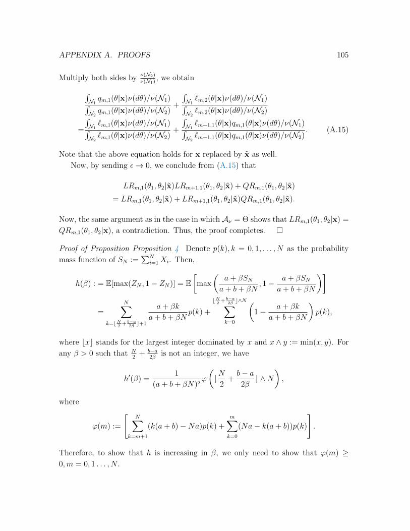
APPENDIX A. PROOFS 105
Multiply both sides by ν(N2)ν(N1)
, we obtain∫N1qm,1(θ|x)ν(dθ)/ν(N1)∫
N2qm,1(θ|x)ν(dθ)/ν(N2)
+
∫N1`m,2(θ|x)ν(dθ)/ν(N1)∫
N2`m,2(θ|x)ν(dθ)/ν(N2)
=
∫N1`m,1(θ|x)ν(dθ)/ν(N1)∫
N2`m,1(θ|x)ν(dθ)/ν(N2)
+
∫N1`m+1,1(θ|x)qm,1(θ|x)ν(dθ)/ν(N1)∫
N2`m+1,1(θ|x)qm,1(θ|x)ν(dθ)/ν(N2)
. (A.15)
Note that the above equation holds for x replaced by x as well.
Now, by sending ε→ 0, we conclude from (A.15) that
LRm,1(θ1, θ2|x)LRm+1,1(θ1, θ2|x) +QRm,1(θ1, θ2|x)
= LRm,1(θ1, θ2|x) + LRm+1,1(θ1, θ2|x)QRm,1(θ1, θ2|x).
Now, the same argument as in the case in which Aν = Θ shows that LRm,1(θ1, θ2|x) =
QRm,1(θ1, θ2|x), a contradiction. Thus, the proof completes.
Proof of Proposition Proposition 4 Denote p(k), k = 0, 1, . . . , N as the probability
mass function of SN :=∑N
i=1 Xi. Then,
h(β) : = E[max(ZN , 1− ZN)] = E[max
(a+ βSNa+ b+ βN
, 1− a+ βSNa+ b+ βN
)]
=N∑
k=bN2
+ b−a2βc+1
a+ βk
a+ b+ βNp(k) +
bN2
+ b−a2βc∧N∑
k=0
(1− a+ βk
a+ b+ βN
)p(k),
where bxc stands for the largest integer dominated by x and x ∧ y := min(x, y). For
any β > 0 such that N2
+ b−a2β
is not an integer, we have
h′(β) =1
(a+ b+ βN)2ϕ
(bN
2+b− a2βc ∧N
),
where
ϕ(m) :=
[N∑
k=m+1
(k(a+ b)−Na)p(k) +m∑k=0
(Na− k(a+ b))p(k)
].
Therefore, to show that h is increasing in β, we only need to show that ϕ(m) ≥0,m = 0, 1 . . . , N .
APPENDIX A. PROOFS 106
Note that
N∑k=0
k(a+ b)p(k) = E[(a+ b)SN ] = (a+ b)E[SN ] = (a+ b)Na
a+ b= aN.
Thus, denoting Y := (a+ b)SN , we have
ϕ(m) = E[(Y − E[Y ])1Y >(a+b)m
]+ E
[(E[Y ]− Y )1Y≤(a+b)m
]= E [Y − E[Y ]] + 2E
[(E[Y ]− Y )1Y≤(a+b)m
]= 2E
[(E[Y ]− Y )1Y≤(a+b)m
].
It is obvious that φ(y) := E [(E[Y ]− Y )1Y≤y] is increasing when y ≤ E[Y ] and
decreasing when y ≥ E[Y ]. Because φ(−∞) = φ(+∞) = 0, we conclude that φ(y) ≥ 0
for any y. Consequently, ϕ(m) ≥ 0 for any m.
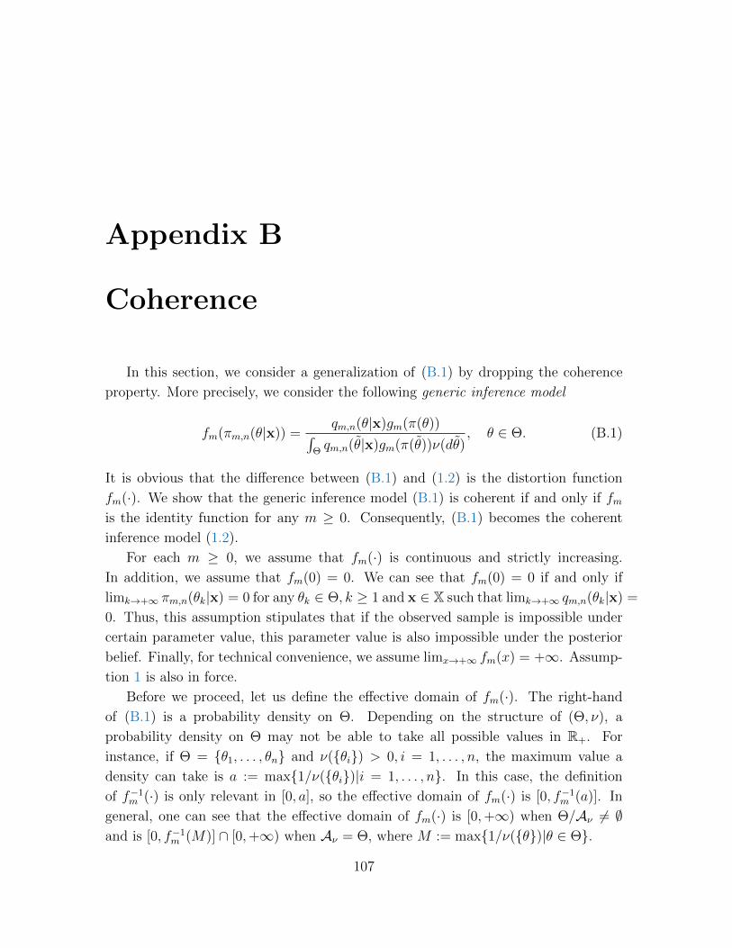
Appendix B
Coherence
In this section, we consider a generalization of (B.1) by dropping the coherence
property. More precisely, we consider the following generic inference model
fm(πm,n(θ|x)) =qm,n(θ|x)gm(π(θ))∫
Θqm,n(θ|x)gm(π(θ))ν(dθ)
, θ ∈ Θ. (B.1)
It is obvious that the difference between (B.1) and (1.2) is the distortion function
fm(·). We show that the generic inference model (B.1) is coherent if and only if fmis the identity function for any m ≥ 0. Consequently, (B.1) becomes the coherent
inference model (1.2).
For each m ≥ 0, we assume that fm(·) is continuous and strictly increasing.
In addition, we assume that fm(0) = 0. We can see that fm(0) = 0 if and only if
limk→+∞ πm,n(θk|x) = 0 for any θk ∈ Θ, k ≥ 1 and x ∈ X such that limk→+∞ qm,n(θk|x) =
0. Thus, this assumption stipulates that if the observed sample is impossible under
certain parameter value, this parameter value is also impossible under the posterior
belief. Finally, for technical convenience, we assume limx→+∞ fm(x) = +∞. Assump-
tion 1 is also in force.
Before we proceed, let us define the effective domain of fm(·). The right-hand
of (B.1) is a probability density on Θ. Depending on the structure of (Θ, ν), a
probability density on Θ may not be able to take all possible values in R+. For
instance, if Θ = θ1, . . . , θn and ν(θi) > 0, i = 1, . . . , n, the maximum value a
density can take is a := max1/ν(θi)|i = 1, . . . , n. In this case, the definition
of f−1m (·) is only relevant in [0, a], so the effective domain of fm(·) is [0, f−1
m (a)]. In
general, one can see that the effective domain of fm(·) is [0,+∞) when Θ/Aν 6= ∅and is [0, f−1
m (M)] ∩ [0,+∞) when Aν = Θ, where M := max1/ν(θ)|θ ∈ Θ.
107
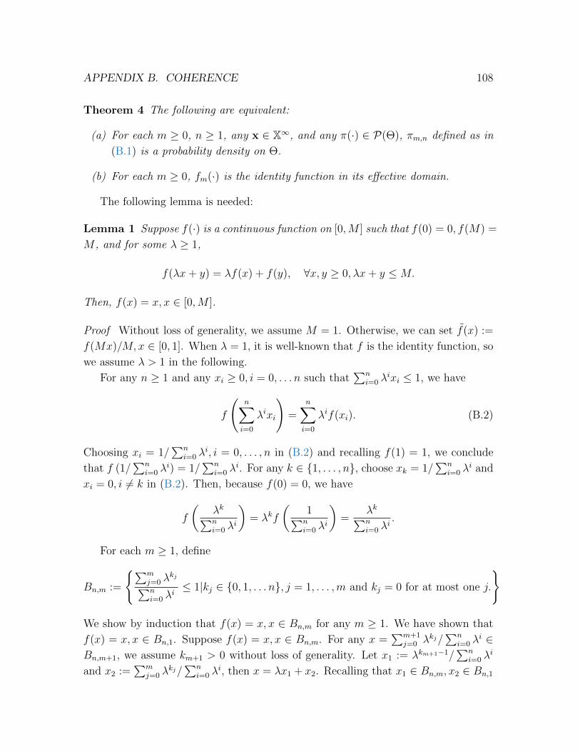
APPENDIX B. COHERENCE 108
Theorem 4 The following are equivalent:
(a) For each m ≥ 0, n ≥ 1, any x ∈ X∞, and any π(·) ∈ P(Θ), πm,n defined as in
(B.1) is a probability density on Θ.
(b) For each m ≥ 0, fm(·) is the identity function in its effective domain.
The following lemma is needed:
Lemma 1 Suppose f(·) is a continuous function on [0,M ] such that f(0) = 0, f(M) =
M , and for some λ ≥ 1,
f(λx+ y) = λf(x) + f(y), ∀x, y ≥ 0, λx+ y ≤M.
Then, f(x) = x, x ∈ [0,M ].
Proof Without loss of generality, we assume M = 1. Otherwise, we can set f(x) :=
f(Mx)/M, x ∈ [0, 1]. When λ = 1, it is well-known that f is the identity function, so
we assume λ > 1 in the following.
For any n ≥ 1 and any xi ≥ 0, i = 0, . . . n such that∑n
i=0 λixi ≤ 1, we have
f
(n∑i=0
λixi
)=
n∑i=0
λif(xi). (B.2)
Choosing xi = 1/∑n
i=0 λi, i = 0, . . . , n in (B.2) and recalling f(1) = 1, we conclude
that f (1/∑n
i=0 λi) = 1/
∑ni=0 λ
i. For any k ∈ 1, . . . , n, choose xk = 1/∑n
i=0 λi and
xi = 0, i 6= k in (B.2). Then, because f(0) = 0, we have
f
(λk∑ni=0 λ
i
)= λkf
(1∑ni=0 λ
i
)=
λk∑ni=0 λ
i.
For each m ≥ 1, define
Bn,m :=
∑mj=0 λ
kj∑ni=0 λ
i≤ 1|kj ∈ 0, 1, . . . n, j = 1, . . . ,m and kj = 0 for at most one j.
We show by induction that f(x) = x, x ∈ Bn,m for any m ≥ 1. We have shown that
f(x) = x, x ∈ Bn,1. Suppose f(x) = x, x ∈ Bn,m. For any x =∑m+1
j=0 λkj/∑n
i=0 λi ∈
Bn,m+1, we assume km+1 > 0 without loss of generality. Let x1 := λkm+1−1/∑n
i=0 λi
and x2 :=∑m
j=0 λkj/∑n
i=0 λi, then x = λx1 + x2. Recalling that x1 ∈ Bn,m, x2 ∈ Bn,1
APPENDIX B. COHERENCE 109
and f(λx1 + x2) = λf(x1) + f(x2), we conclude that
f(x) = f(λx1 + x2) = λf(x1) + f(x2) = λx1 + x2 = x.
We have shown that f(x) = x for all x ∈ B := ∪∞n=0Bn where B0 := 0, 1 and
Bn := ∪∞m=1Bn,m, n ≥ 1. Next, we show that B is dense in [0, 1]. For any x0 ∈ [0, 1]
and any ε > 0, choose n ≥ 1 such that λ∑ni=0 λ
i < ε. If x0 ≤ 1∑ni=0 λ
i , then |x0 − 0| < ε.
Otherwise, let k1 be the largest k such that λk∑ni=0 λ
i ≤ x0. Denote x1 := λk1∑ni=0 λ
i , then
x1 ∈ Bn and x0 − x1 ≥ 0. If k1 = 0, then x0 − x1 ≤ λ∑ni=0 λ
i . Otherwise, let k2
be the largest k such that λk∑ni=0 λ
i ≤ x0 − x1 and denote x2 := x1 + λk2∑ni=0 λ
i . Then,
x2 ∈ Bn and x0 − x2 ≥ 0. If k2 = 0, then x0 − x2 ≤ λ∑ni=0 λ
i . Otherwise, let k3 be the
largest k such that λk∑ni=0 λ
i ≤ x0 − x2 and denote x3 := x2 + λk3∑ni=0 λ
i . Repeating this
construction, after finite number of steps, e.g., `, we must have k` = 0. As a result,
0 ≤ x0 − x` ≤ λ∑ni=0 λ
i < ε and x` ∈ Bn. Thus, B is dense in [0, 1].
Because f(x) = x, x ∈ B, B is dense in [0, 1], and f(·) is continuous on [0, 1], we
have f(x) = x, x ∈ [0, 1].
Proof of Theorem 4 The direction (b)⇒(a) is obvious, so we only need to prove
(a)⇒(b). Let us fix m ≥ 0. We first consider the case in which Θ/Aν 6= ∅. In
this case, ν(Θ/Aµ) ∈ (0,+∞] because Θ/Aµ is open and the support of ν is Θ.
Fix any x ∈ X∞, then we can find θ0 ∈ Θ/Aν such that qm,n(θ0|x) > 0. Because
qm,n is continuous in θ, we can find a neighbourhood of θ0, denoted as N0, such that
N0 ⊂ Θ/Aν and 1/C ≤ qm,n(θ|x) ≤ C, ∀θ ∈ N0 for some C > 0. Because the support
of ν is Θ, we have ν(N0) ∈ (0,+∞]. Because ν is σ-finite, we can find N1 ⊂ N0 such
that ν(N1) ∈ (0,+∞).
Next, we show that for any bounded density function p(·) on Θ (i.e., 0 ≤ p(θ) ≤K, ∀θ ∈ Θ for some K > 0 and
∫Θp(θ)ν(dθ) = 1) such that p(θ) = 0, θ ∈ Θ/N1, we
can construct a prior density π(·) such that
p(θ) =qm,n(θ|x)gm(π(θ))∫
Θqm,n(θ|x)gm(π(θ))ν(dθ)
, ∀θ ∈ Θ. (B.3)
To this end, for each z ≥ 0, define
hz(θ) := g−1m
(zp(θ)
qm,n(θ|x)
)1N1(θ), θ ∈ Θ.
Because 1/C ≤ qm,n(θ|x) ≤ C, ∀θ ∈ N1, hz(·) is well-defined. Furthermore, because
APPENDIX B. COHERENCE 110
ν(N1) < +∞ and p(·) is bounded, the monotone convergence theorem shows that
λ(z) :=∫
Θhz(θ)ν(dθ) is continuous in z. Because gm(0) = 0, we have λ(0) = 0.
On the other hand, because ν(N1) > 0, we have limz→+∞ λ(z) = +∞. As a result,
there exist z0 > 0 such that λ(z0) = 1. Define π(θ) = hz0(θ), θ ∈ Θ, then π is a
probability density. Furthermore, thanks to gm(0) = 0, one can check that p(θ) ∝qm,n(θ|x)gm(π(θ)) and thus (B.3) holds.
It is assumed that πm,n defined as in (B.1) is a probability density for any π ∈P(Θ). In addition, any bounded density function p(·) such that p(θ) = 0, θ ∈ Θ/N1
can be constructed in the form of (B.3) from some prior density π. Therefore, we
conclude that for any such p(·), the function πm,n solved from
fm(πm,n(θ|x)) = p(θ), θ ∈ Θ (B.4)
must satisfy∫
Θπm,n(θ|x)ν(dθ) = 1.
Now, for any y ≥ 1/ν(N1), because ν has no atom on Θ/Aν , we can find N2 ⊂ N1
such that ν(N2) = 1/y; see for instance Follmer and Schied [2004, Proposition A.27].
Define p(θ) := y1N2(θ), θ ∈ Θ. One can see that p(·) is a bounded density on Θ and
takes zero outside N2. Thanks to fm(0) = 0, πm,n(θ|x) defined as in (B.4) can be
solved as follows:
πm,n(θ|x) = f−1m (p(θ)) = f−1
m (y)1N2(θ), θ ∈ Θ.
As a result,
1 =
∫Θ
πm,n(θ|x)ν(dθ) = f−1m (y)ν(N2) = f−1
m (y)/y,
which shows that f−1m (y) = y.
For y ∈ (0, 1/ν(N1)), consider p(θ) := y1N2(θ) + y1N1/N2(θ), θ ∈ Θ, where N2 is
chosen to be a subset of N1 such that ν(N2) = 12ν(N1) and y := 2
ν(N1)− y. One can
verify that p(·) is a bounded density function. Furthermore, because y < 1/ν(N1),
we have y > 1/ν(N1) and thus f−1m (y) = y. Consider the corresponding πm,n(θ|x)
defined through (B.4). One can calculate that
πm,n(θ|x) = f−1m (p(θ)) = f−1
m (y)1N2(θ) + f−1m (y)1N1/N2(θ), θ ∈ Θ.
APPENDIX B. COHERENCE 111
Then,
1 =
∫Θ
πm,n(θ|x)ν(dθ) = f−1m (y)ν(N2) + f−1
m (y)ν(N1/N2) =ν(N1)
2(f−1m (y) + f−1
m (y)).
As a result,
f−1m (y) =
2
ν(N1)− f−1
m (y) =2
ν(N1)− y =
2
ν(N1)−(
2
ν(N1)− y)
= y.
To summarize, we have shown that when Θ/Aµ 6= ∅, f−1m (y) = y for any y > 0,
i.e., fm(·) is the identity function.
Next, we consider the case in which Aµ = Θ. Fixing any x ∈ X∞ and any
mutually different θ1, θ2, θ3, we have qm,n(θi|x0,m) > 0, i = 1, 2, 3. Applying a similar
argument to the one used in the case in which Θ/Aν 6= ∅, we can show that for any
bounded density p(·) with support on θ1, θ2, θ3, there exist a prior density π such
that (B.3) holds. As a result, for any such p(·), πm,n(θ|x) solved through (B.4) must
satisfy∫
Θπm,n(θ|x)ν(dθ) = 1. Consequently, for any pi ≥ 0, i = 1, 2, 3 such that∑3
i=1 piν(θi) = 1, by setting p(θi) = pi, i = 1, 2, 3, we have
1 =
∫Θ
πm,n(θ|x)ν(dθ) =
∫Θ
f−1m (p(θ))ν(dθ) =
3∑i=1
f−1m (pi)ν(θi). (B.5)
In particular, f−1m
(1
ν(θi)
)= 1, i = 1, 2, 3. Without loss of generality, we assume
1ν(θ1) ≤
1ν(θ2) ≤
1ν(θ3) . In the following, we show that f−1
m (y) = y, 0 ≤ y ≤ 1ν(θ3) .
For any x and y such that xν(θ2)+yν(θ3) ≤ 1, by setting p1 = 1−xν(θ2)−yν(θ3)ν(θ1) ,
p2 = x, p3 = y, p1 = 1−xν(θ2)−yν(θ3)ν(θ1) , p2 = 0, and p3 = ν(θ2)
ν(θ3)x+ y, we have
f−1m (x)ν(θ2) + f−1
m (y)ν(θ3) = 1− f−1m
(1− xν(θ2)− yν(θ3)
ν(θ1)
)= f−1
m
(ν(θ2)ν(θ3)
x+ y
)ν(θ3).
Defining λ := ν(θ2)ν(θ3) , we conclude that for any x, y ≥ 0 such that λx + y ≤ 1
ν(θ3) ,
f−1m (λx+ y) = λf−1
m (x) + f−1m (y). Lemma 1 shows that f−1
m (·) is the identity function
on[0, 1
ν(θ3)
]. Because θi, i = 1, 2, 3 are arbitrarily chosen in Aν , fm(·) is the identity
function in its effective domain.
Appendix C
The Two-Element Case
In this chapter, we assume that Θ = θ1, θ2 and Assumption 1-(ii) and (iii) hold.
C.1 Main Results in Chapter 1
Corollary 1 For any fixed m ≥ 0 and n ≥ 1, consider two pairs of pseudo-likelihood
and distortion, (qm,n(θ|x), gm) and (q′m,n(θ|x), g′m), that satisfy Assumption 1. Then,
(qm,n(θ|x), gm) and (q′m,n(θ|x), g′m) lead to the same posterior density πm,n in the co-
herent inference model (1.2) for any prior density π and any sample sequence x if
and only if (i) gm(x)/gm(y) = g′m(x)/g′m(y) for any x, y > 0 such that xν(θ1) +
yν(θ2) = 1 and (ii) for any x ∈ X∞, there exists Cm,n(x) > 0 such that qm,n(θ|x) =
Cm,n(x)q′m,n(θ|x) for all θ ∈ Θ.
Proof Because Θ = θ1, θ2, the distribution of θ is simply determined by the odds of
θ1 in favor of θ2 under this distribution. The posterior odds in the coherent inference
model is
Om,n(x) :=πm,n(θ1|x)
πm,n(θ1|x)=qm,n(θ1|x)gm(π(θ1))
qm,n(θ1|x)gm(π(θ2)).
We first prove sufficiency. Denote Om,n(x) and O′m,n(x) as the posterior odds in
112
APPENDIX C. THE TWO-ELEMENT CASE 113
(1.2) with (qm,n(θ|x), gm) and (q′m,n(θ|x), g′m), respectively. Then,
Om,n(x) =qm,n(θ1|x)gm(π(θ1))
qm,n(θ1|x)gm(π(θ2))
=Cm,n(x)q′m,n(θ1|x)g′m(π(θ1))
Cm,n(x)q′m,n(θ2|x)g′m(π(θ2))
= O′m,n(x).
Next, we prove the necessity. For Om,n(x) and O′m,n(x) to be equal for any x and
any π, we must have
gm(π(θ1))
gm(π(θ2))/g′m(π(θ1))
g′m(π(θ2))=q′m,n(θ1|x)
q′m,n(θ2|x)/qm,n(θ1|x)
qm,n(θ1|x)
for any π. Because fixing x, (π(θ1), π(θ2)) can take any pair of values (x, y) such that
x, y > 0 such that xν(θ1) + yν(θ2) = 1, and the right-hand side does not depend
on (x, y), we immediately conclude that
gm(x)
gm(y)/g′m(x)
g′m(y)= C, ∀x > 0, y > 0 such that xν(θ1) + yν(θ2) = 1
for some constant C. By setting x = y, we immediately conclude that C = 1. This
further implies that
q′m,n(θ1|x)
q′m,n(θ2|x)/qm,n(θ1|x)
qm,n(θ1|x)= 1, ∀x,
which is equivalent to condition (ii) in the Corollary.
Corollary 2 The coherent inference model (1.2) is processing consistent if and only
if
(i) for each m ≥ 1, gm(x)/gm(y) = x/y for any x, y > 0 such that xν(θ1) +
yν(θ2) = 1; and
(ii) for each m ≥ 1 and n ≥ 1 and any x ∈ X∞, there exists Cm,n(x) > 0 such that
(1.4) holds.
Proof Because Θ = θ1, θ2, the distribution of θ is simply determined by the odds of
θ1 in favor of θ2 under this distribution. The posterior odds in the coherent inference
APPENDIX C. THE TWO-ELEMENT CASE 114
model is
Om,n(x) :=πm,n(θ1|x)
πm,n(θ1|x)=qm,n(θ1|x)gm(π(θ1))
qm,n(θ1|x)gm(π(θ2)).
We first prove sufficiency. Denote Om,n(x; π0) and O0,m+n(x; π0), respectively as
the posterior odds in (1.2) when processing x0,m and xm,n sequentially and when
processing x0,m+n as a group. Denote π0,m(θ|x; π0) as the posterior density obtained
after processing x0,m as a group. Then,
Om,n(x; π0) =qm,n(θ1|x)gm(π0,m(θ1|x; π0))
qm,n(θ1|x)gm(π0,m(θ2|x; π0))
=qm,n(θ1|x)π0,m(θ1|x; π0)
qm,n(θ1|x)π0,m(θ2|x; π0)
=qm,n(θ1|x)q0,m(θ1|x)g0(π0(θ1))
qm,n(θ1|x)q0,m(θ1|x)g0(π0(θ2))
=Cm,n(x)−1q0,m+n(θ1|x)g0(π0(θ1))
Cm,n(x)−1q0,m+n(θ2|x)g0(π0(θ2))
= O0,m+n(x; π0).
Next, we prove necessity. For Om,n(x; π0) and O0,m+n(x; π0) to be equal for any
π0, we must have
qm,n(θ1|x)gm(π0,m(θ1|x; π0))
qm,n(θ1|x)gm(π0,m(θ2|x; π0))=q0,m+n(θ1|x)g0(π0(θ1))
q0,m+n(θ2|x)g0(π0(θ2))
for any π0, which is the case if and only if
qm,n(θ1|x)q0,m(θ1|x)gm(π(θ1))
qm,n(θ1|x)q0,m(θ1|x)gm(π(θ2))=q0,m+n(θ1|x)π(θ1)
q0,m+n(θ2|x)π(θ2)(C.1)
holds for any density π because (i)
π0,m(θ1|x; π0)
π0,m(θ2|x; π0)=q0,m(θ1|x)g0(π0(θ1))
q0,m(θ2|x)g0(π0(θ2))
and (ii) for any fixed x and any density π, we can find π0 such that π0,m(θ|x; π0) =
π(θ),∀θ ∈ Θ. Note that (C.1) holds for any π if and only if
qm,n(θ1|x)q0,m(θ1|x)
qm,n(θ1|x)q0,m(θ1|x)/q0,m+n(θ1|x)
q0,m+n(θ2|x)=π(θ1)
π(θ2)/gm(π(θ1))
gm(π(θ2))
APPENDIX C. THE TWO-ELEMENT CASE 115
for any density π. Because fixing x,(π(θ1), π(θ2)
)can take pair of values (x, y) for
any x, y such that x > 0, y > 0, and xν(θ1) + yν(θ2) = 1, we immediately
conclude that
x
y/gm(x)
gm(y)= C, ∀x > 0, y > 0 such that xν(θ1) + yν(θ2) = 1.
for some constant C. By setting x = y, we further conclude C = 1, thus obtaining
the necessary condition (i). We further conclude that
qm,n(θ1|x)q0,m(θ1|x)
qm,n(θ1|x)q0,m(θ1|x)/q0,m+n(θ1|x)
q0,m+n(θ2|x)= 1
for any x, and this is the case if and only if the necessary condition (ii) holds.
Corollary 3 Denote the one-step pseudo-likelihood qm,1(θ|x) in the coherent infer-
ence model as qm,1(θ|x0,m, xm+1).
(i) The coherent inference model (1.2) is false Bayesian in the strong sense if and
only if it is processing consistent, g0(x)/g0(y) = x/y for any x, y > 0 such
that xν(θ1) + yν(θ2) = 1, and, for each m ≥ 0, there exists a measurable
function ϕm(x0,m, x) > 0,x0,m ∈ Xm, x ∈ X such that (1.10) holds.
(ii) The coherent inference model (1.2) is false Bayesian in the weak sense if and
only if it is processing consistent and, for each m ≥ 1, there exists a measurable
function ϕm(x0,m, x) > 0,x0,m ∈ Xm, x ∈ X such that (1.10) holds.
Proof The proof of this Corollary follows from the proof of Corollary 2 and the proof
of Theorem 2.
C.2 Generic Inference Model
Next, we study the issue of when the generic inference model B.1 is coherent in
the two-element case.
Corollary 4 The generic inference model B.1 is coherent, i.e., for each m ≥ 0,
n ≥ 1, any x ∈ X∞, and any π(·) ∈ P(Θ), πm,n defined as in (B.1) is a probability
density on Θ, if and only if for each m ≥ 0 and x > 0, y > 0 such that xν(θ1) +
yν(θ2) = 1, we have f−1m (x)ν(θ1) + f−1
m (y)ν(θ2) = 1.
APPENDIX C. THE TWO-ELEMENT CASE 116
Proof Following the proof of Theorem 4, we can show that for any density p, we can
find a prior density π such that (B.3) holds. Consequently, model B.1 is coherent if
and only if∫
Θf−1m (p(θ))ν(dθ) = 1 for any density p. Because Θ = θ1, θ2, the proof
completes.
Let us comment that the condition that f−1m (x)ν(θ1) + f−1
m (y)ν(θ2) = 1 for
any x > 0, y > 0 such that xν(θ1) + yν(θ2) = 1 does not imply that fm is the
identity function. For example, suppose ν(θ1) = ν(θ2) = 1, the above condition
is satisfied by f on [0, 1] such that f(x) = f(1− x), x ∈ [0, 1/2].
C.3 Main Results in Chapter 2
Finally, we comment that the necessary condition (i) in Corollary 2 stipulates that
the distortion gm does not affect the prior odds of θ1 in favor of θ2. Thus, even in
the case in which Θ = θ1, θ2, we can assume without loss of generality that in a
processing-consistent, coherent inference model, gm is a linear function for any m ≥ 1,
i.e., the necessary condition (i) in Theorem 1 holds. Consequently, all the results in
Section 2.2 still hold in this case.


