/ee/lecceq.tex
Nuclei beyond the independent particle description:
The importance of correlations
Ingo Sick
Historical development of nuclear physics
strongly influenced by mean-field ideas
till today main approach to describe nuclei
Main assumption: nucleons move in mean field
field created by average interaction with all other nucleons
individual nucleon moves independently of others
residual interactions incorporated perturbatively
Consequences:
nuclei have many similarities to atoms
appearance of shells, magic numbers, ..
existence of quasi-particle (QP) orbits
Mean field description
reasonably successful
when use fitted effective interactions, fitted mean field
can explain many features of nuclei
amazing that works, given properties of N-N-interaction
But: fitted parameters, limited to selected observables
for new observable need different parameters
connection to underlying N-N interaction remote
”easy” calculations, but not very satisfactory
More fundamental approach: start from N-N interaction
solve Schrodinger equation for A nucleons interacting with VNN
Difficulty:
N-N interaction very complicated
spin- and (angular)-momentum dependent
has strong short range repulsion
⇒ solution of n-body Schrodinger equation very difficult
Exact (numerical) solution for known VNN :
feasible for infinite nuclear matter (NM)
Bethe-Bruckner-Goldstone theory
Correlated Basis Function (CBF) theory
feasible for light nuclei (A<12)
Faddeev, Hyperspherical, Variational MC
gradually also feasible for heavier nuclei
Fermi Hypernetted Chain calculations
Advantage:
basis = N-N interaction known from N-N scattering
applicable to a priori all nuclei
no free parameters
decisive for predictions at higher densities as occur e.g. in stars
Main difference to mean-field
account for short-range N-N correlations
short-range interactions leads to scattering of N to orbits E ≫ EFshort-range interactions leads to scattering of N to orbits k ≫ kFpartial depletion for E < EF , k < kF
for quantitative understanding
correlations absolutely crucial

Ideal approach to expose correlations: CBF theory
appear explicitly as variational functions f(rij) in wave function
|N) = G|N ], G = S∏
j>i
F (i, j), F (i, j) =∑
nfn(rij)O
n(i, j)
Effect of correlations
on components of potential on f(rij)
|N ] = MF state
O = operators of VNNf = correlation
functions
variationally det.
correlation hole for some components, short-range enhancements for others
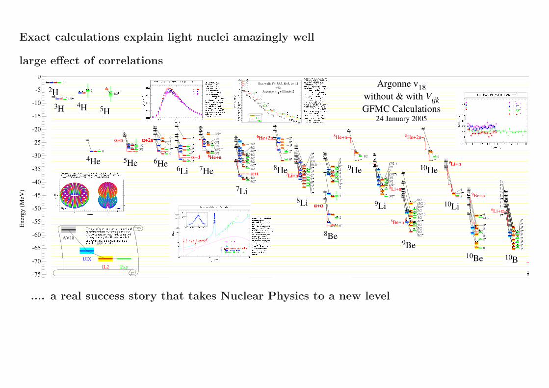
Exact calculations explain light nuclei amazingly well
large effect of correlations
.... a real success story that takes Nuclear Physics to a new level

Important difference quasi-particle ↔ correlated strength
QP wave functions: R(k) falls quickly at large k
correlated strength: has long tail towards large k
example: 4He from Variational Monte Carlo
i.e. exact calculation for realistic NN-interaction
2222 QP orbital, observed e.g. in 4He(e, e′p)3H
drops off rapidly at large k
3333 correlated strength in continuum at large E
falls off much less quickly, dominates large-k totally
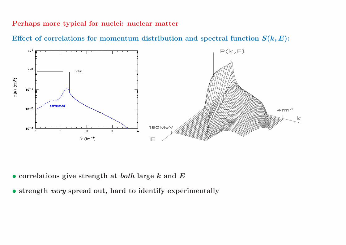
Perhaps more typical for nuclei: nuclear matter
Effect of correlations for momentum distribution and spectral function S(k,E):
• correlations give strength at both large k and E
• strength very spread out, hard to identify experimentally
• correlated N have ∼20% probability (NM),
but give 37% of removal energy
47% of kinetic energy
(CBF calculation of Benhar, Fabrocini, Fantoni 1989)
⇒ mean-field approach cannot work
exception(?): differences of energies, spect. factors
insight for time being lost on shell-model community
calculations of ever increasing sophistication
ignoring 20% of nucleons
e.g. review Talmi, ”50 years of shell model”, 275pages
not one word on 20%, 37%, 47%
correlated N even more crucial for:
2N-dependent processes, MEC
enhancement of integrated transverse (e,e’) strength
NM study of A. Fabrocini
transverse sum rule in 3He, 4He, J.Carlson et al.
effect of MEC with correlations 8 times larger
only with correlations can explain data
Analogous studies of liquid Helium
calculation easier, no spin-dependence
Lennard-Jones potential, r−12 − r−6, even more repulsive at small r
⇒ even stronger correlations
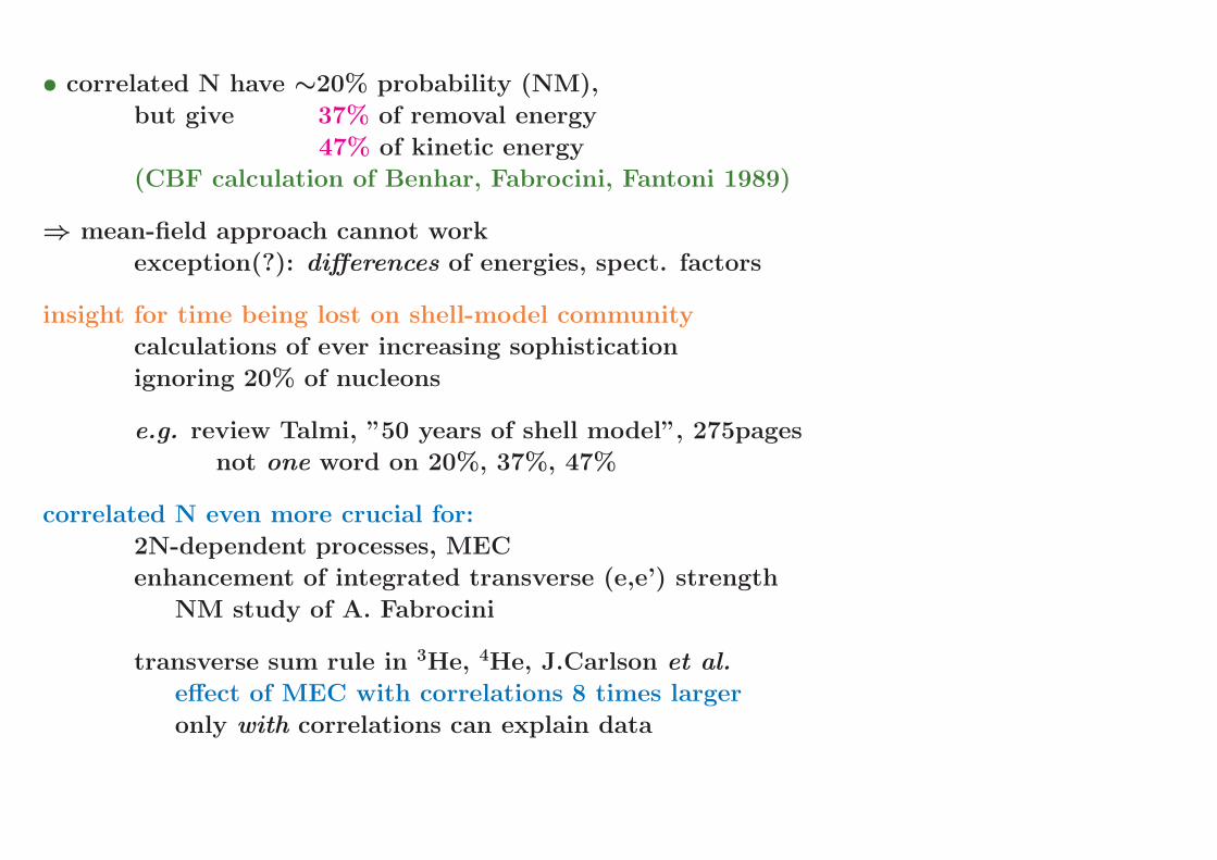
But
find quasi-particle states for k < kFwith much reduced occupation
occupation of MF states ∼ 30%
= size of discontinuity at kFrest moved to k > kF mainly
”depopulation” of MF states
= main consequence for MF
Shown by Moroni et al.
via calculations for L3He and L4He
depopulation similar for bosonic/fermionic systems
mainly consequence of short-range VNN , not Pauli principle
Finite systems
more complicated
”occupation” requires concept of ”orbit”
not a priori obvious which one:
mean field, overlap, natural, ....?
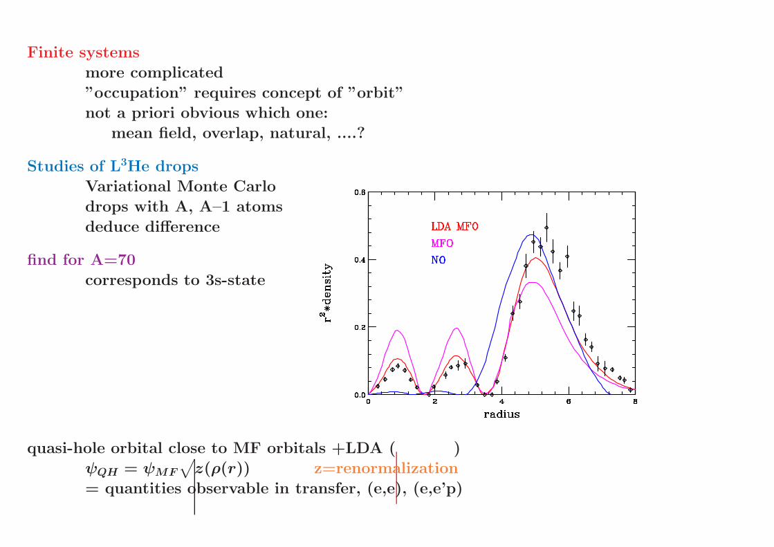
Studies of L3He drops
Variational Monte Carlo
drops with A, A–1 atoms
deduce difference
find for A=70
corresponds to 3s-state
quasi-hole orbital close to MF orbitals +LDA ( )
ψQH = ψMF
√
z(ρ(r)) z=renormalization
= quantities observable in transfer, (e,e), (e,e’p)
main message
in nuclei and LHe find orbits ∼ quasi-particle states
R(r), R(k) ± as given by mean-field models
observed in transitions to E < 10 MeV
but
single particle states have partial occupation
spectroscopic factors (= overlap with IPSM wave functions) <1
rest of strength at very large k,E
large effect of correlated strength on Ekin, Eint
experimental observation of depopulation?
long in coming
suitable experiments not available

Traditional tools used to measure spectroscopic factors s:
(d,3He), (p,d), ..., (p,2p), ..., (e,e’p)
most extensive source of information: transfer reactions
What do they really measure?
consider radial sensitivity of probes, for Pb
sensitivity of (e,e) flat, (p,2p) further outside than (e,e’p) [more absorption],
transfer reactions measure asymptotic norm, not s
should really only quote this quantity! ... but somehow people want s

Why want s?
better intuitive meaning than asymptotic norm
(typical) HO-based calculations only give s
If want s from transfer: suffer from strong dependence on R(r)
s typically changes 10% for a 1% change in rms-radius of R(r)
since rms-radius not known → s rather arbitrary
Past prejudice
∑
i
si, summed over final states i, gives occupation np,h (pickup, transfer)
nparticle + nhole = 1, i.e. 2j+1 particles in state j
chose R(r) such as to get 1
Result
find small values for nhfind np close to 1
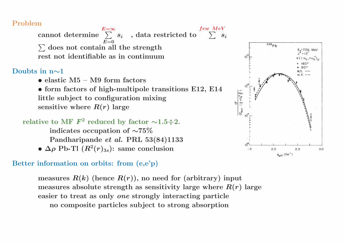
Problem
cannot determineE=∞∑
E=0
si , data restricted tofew MeV
∑
si∑
does not contain all the strength
rest not identifiable as in continuum
Doubts in n∼1
• elastic M5 – M9 form factors
• form factors of high-multipole transitions E12, E14
little subject to configuration mixing
sensitive where R(r) large
relative to MF F 2 reduced by factor ∼1.5÷2.
indicates occupation of ∼75%
Pandharipande et al. PRL 53(84)1133
• ∆ρ Pb-Tl (R2(r)3s): same conclusion
Better information on orbits: from (e,e’p)
measures R(k) (hence R(r)), no need for (arbitrary) input
measures absolute strength as sensitivity large where R(r) large
easier to treat as only one strongly interacting particle
no composite particles subject to strong absorption

Data
early results from Saclay:
find orbits with R(k) ∼ MF
MF also applicable to nuclear interior
find occupation n ∼0.7
n not taken very seriously
doubts about DWBA treatment
... which however was OK
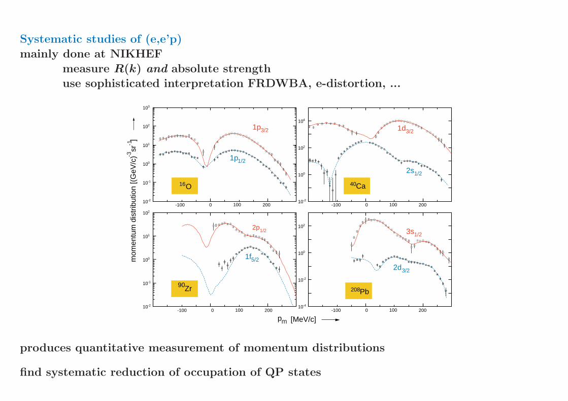
Systematic studies of (e,e’p)
mainly done at NIKHEF
measure R(k) and absolute strength
use sophisticated interpretation FRDWBA, e-distortion, ...
10-2
10-1
100
101
102
103
1p3/2
1p1/2
16O
10-2
100
102
104
1d3/2
2s1/2
-100 0 20010-2
10-1
100
101
102
p [MeV/c]
mom
entu
m d
istr
ibut
ion
[(G
eV/c
) s
r ]
2p1/2
1f5/2
10-4
10-2
100
102
208Pb
3s1/2
2d3/2
90Zr
40Ca
100 -100 0 200100
-100 0 200100 -100 0 200100
m
-3-1
produces quantitative measurement of momentum distributions
find systematic reduction of occupation of QP states
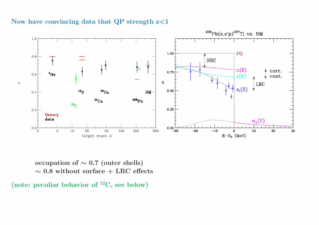
Now have convincing data that QP strength z<1
occupation of ∼ 0.7 (outer shells)
∼ 0.8 without surface + LRC effects
(note: peculiar behavior of 12C, see below)
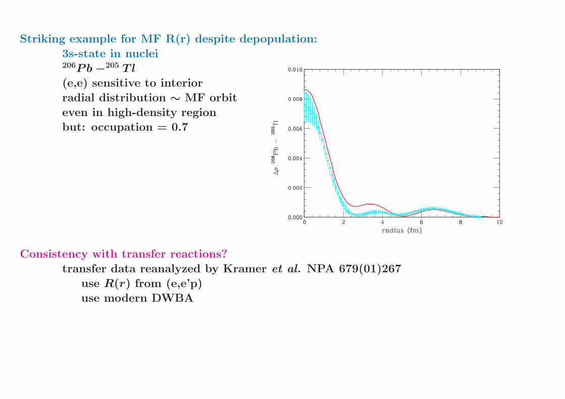
Striking example for MF R(r) despite depopulation:
3s-state in nuclei206Pb−205 T l
(e,e) sensitive to interior
radial distribution ∼ MF orbit
even in high-density region
but: occupation = 0.7
Consistency with transfer reactions?
transfer data reanalyzed by Kramer et al. NPA 679(01)267
use R(r) from (e,e’p)
use modern DWBA
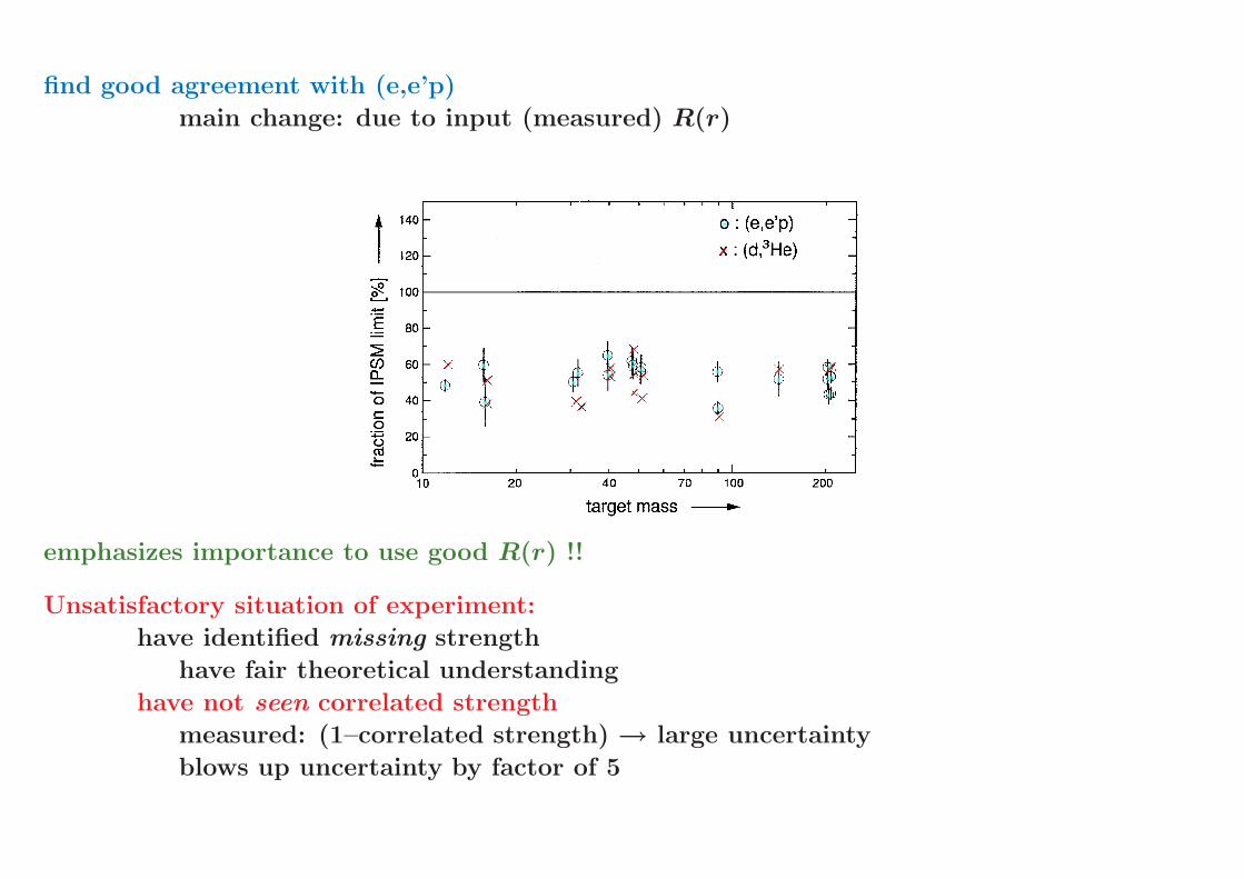
find good agreement with (e,e’p)
main change: due to input (measured) R(r)
emphasizes importance to use good R(r) !!
Unsatisfactory situation of experiment:
have identified missing strength
have fair theoretical understanding
have not seen correlated strength
measured: (1–correlated strength) → large uncertainty
blows up uncertainty by factor of 5

Past attempts to identify strength at large k
• reactions of type (x,p)
low momentum transfer from x, observe high momentum p
e.g. (γ,p), (p,p) with high-momentum backward p
problem: Amado+Woloshyn, 1977
• in limit q→0 FSI cancels IA term from high-k component (orthogonality!)
no quantitative interpretation possible
(applies also to (p,2p), .. )
• (e,e’) at large q, low ω
~k
~q~k + ~q
idea: small ω ∼ (~k + ~q)2/2m, large ~q → ~k ∼ −~q, large
problem: FSI (e.g. 3He(e,e’), PWIA = )
• see Benhar, Fabrocini, Fantoni,... (1991)
provide first treatment of FSI using Glauber, find that dominates
but: not entirely satisfactory, still in the works
for either case: cannot address large k anyway as strength is at large E
... an insight that has yet to sink in
Best tool to measure strength at large k and large E:
(e,e′p) at large q
can minimize effect FSI
can treat reliably via Glauber
complications:
• must look at large E
not large k and small E as done initially and ± all existing experiments
• strength spread out over 100-200MeV
small in given (k,E)-bin
very hard to observe
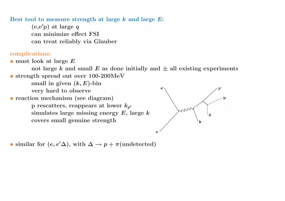
• reaction mechanism (see diagram)
p rescatters, reappears at lower kp′
simulates large missing energy E, large k
covers small genuine strength
• similar for (e, e′∆), with ∆ → p+ π(undetected)
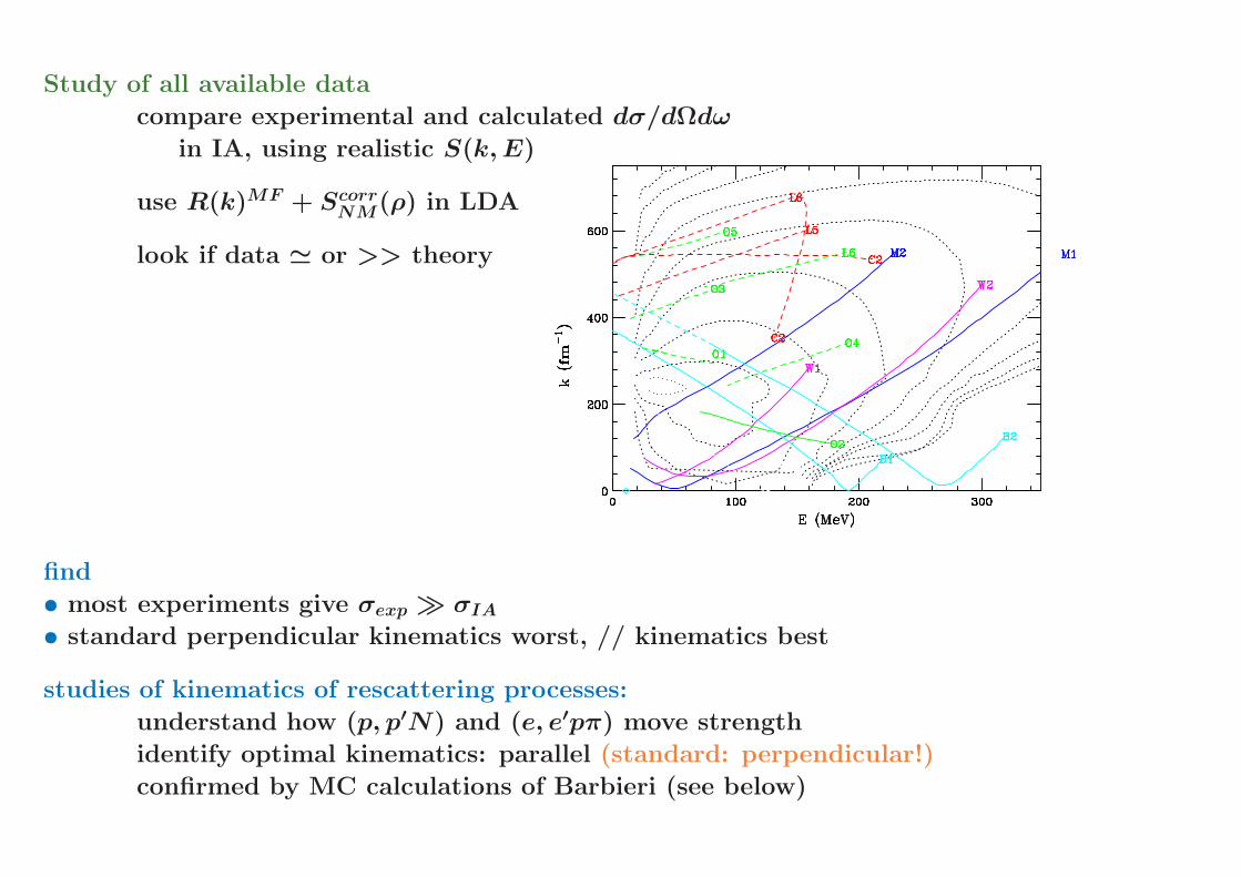
Study of all available data
compare experimental and calculated dσ/dΩdω
in IA, using realistic S(k,E)
use R(k)MF + ScorrNM(ρ) in LDA
look if data ≃ or >> theory
find
• most experiments give σexp ≫ σIA• standard perpendicular kinematics worst, // kinematics best
studies of kinematics of rescattering processes:
understand how (p, p′N) and (e, e′pπ) move strength
identify optimal kinematics: parallel (standard: perpendicular!)
confirmed by MC calculations of Barbieri (see below)
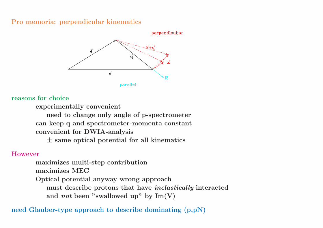
Pro memoria: perpendicular kinematics
reasons for choice
experimentally convenient
need to change only angle of p-spectrometer
can keep q and spectrometer-momenta constant
convenient for DWIA-analysis
± same optical potential for all kinematics
However
maximizes multi-step contribution
maximizes MEC
Optical potential anyway wrong approach
must describe protons that have inelastically interacted
and not been ”swallowed up” by Im(V)
need Glauber-type approach to describe dominating (p,pN)

Detector stack:
2 drift chambers 4 scintillator planes 1 Cerenkov
HMS
SOS
Q Q Q D
D
D
e
e′
p′
3.2 GeV
0.85-1.7 GeV/c
2.05-2.75 GeV/c
Target spectrometer
(e,e’p) experiment
JLab hall C:
Daniela Rohe et al.

Can achieve with JLab:
large q → low FSI, treatable with Glauber
acceptable true/accidental ratio
despite unfavorable (//) kinematics
Tests
in single-particle region, kinematics with same Ep′ as production runs
use: T=0.6... (Benhar+Pieper), integrate over E <80MeV
find: occupation agrees with CBF S(k,E)

Results for correlated region
0.1 0.2 0.3 0.4E
m (GeV)
1e-13
1e-12
1e-11
1e-10
S(E
m,p
m)
[MeV
-4 s
r-1]
0.1700.2100.2500.2900.3300.3700.4100.4500.4900.5300.1700.2100.5700.6100.650
Spectral function for C using ccparallel: kin3, kin4, kin5
pm
(GeV/c)Em
= p2
m2 M
p
main observation on E-dependence
maximum of S(k,E) of theories at too large E
understood by recent calculation of Muther+Polls?
selfconsistent GF, ladder approximation, finite T

Momentum dependence
0.2 0.4 0.6p
m [GeV/c]
10-3
10-2
10-1
n(p m
) [f
m3 s
r-1]
parallel
CBF theoryGreens function approachexp. using cc1(a)exp. using cc
⇒ theory and experiment ± agree
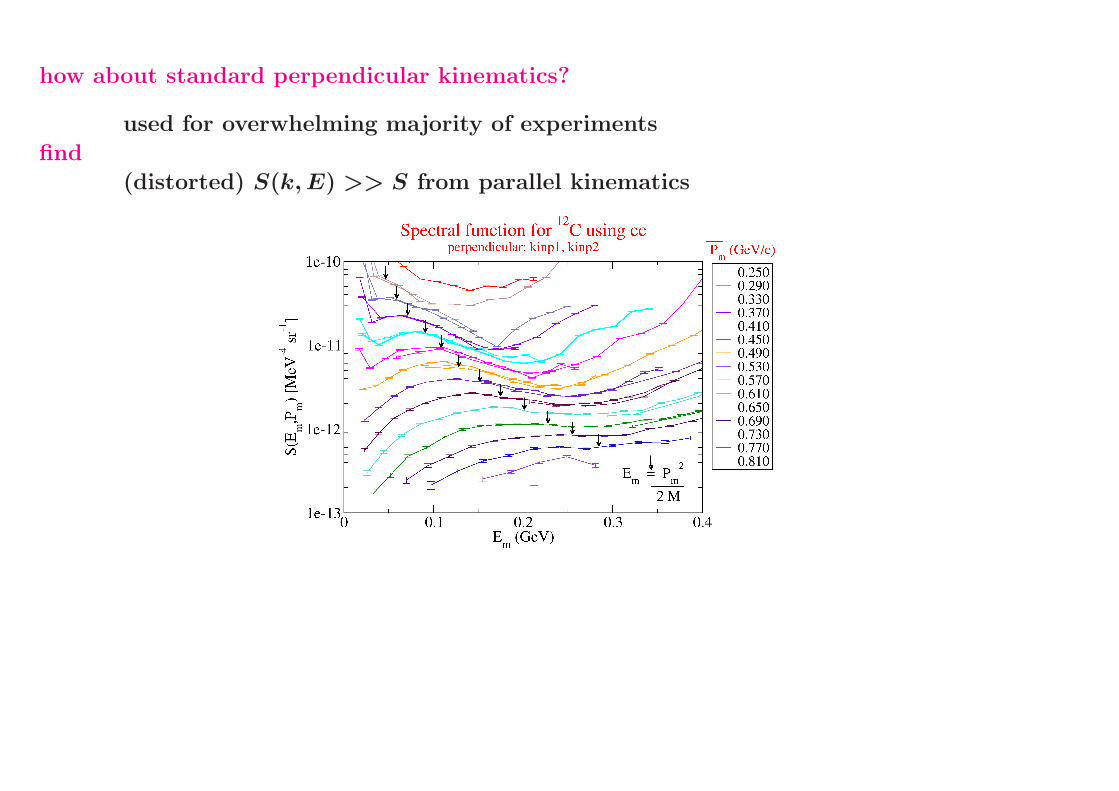
how about standard perpendicular kinematics?
used for overwhelming majority of experiments
find
(distorted) S(k,E) >> S from parallel kinematics
ckp1p2_e01trec16n_cc1on_nice.agr
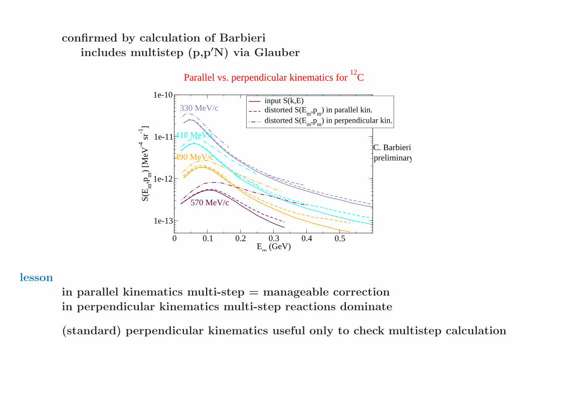
confirmed by calculation of Barbieri
includes multistep (p,p′N) via Glauber
0 0.1 0.2 0.3 0.4 0.5E
m (GeV)
1e-13
1e-12
1e-11
1e-10
S(E
m,p
m)
[MeV
-4 s
r-1]
input S(k,E) distorted S(E
m,p
m) in parallel kin.
distorted S(Em
,pm
) in perpendicular kin.
Parallel vs. perpendicular kinematics for 12
C
330 MeV/c
410 MeV/c
490 MeV/c
570 MeV/c
C. Barbieri,preliminary
lesson
in parallel kinematics multi-step = manageable correction
in perpendicular kinematics multi-step reactions dominate
(standard) perpendicular kinematics useful only to check multistep calculation
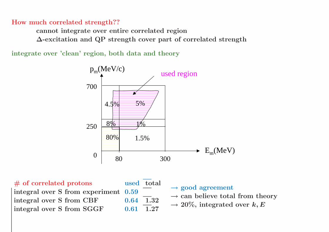
How much correlated strength??
cannot integrate over entire correlated region
∆-excitation and QP strength cover part of correlated strength
integrate over ’clean’ region, both data and theory
80%
250
80 300
1.5%
5%
700
0
4.5%
8% 1%
Em(MeV)
pm(MeV/c)used region
# of correlated protons used total
integral over S from experiment 0.59
integral over S from CBF 0.64 1.32
integral over S from SGGF 0.61 1.27
→ good agreement
→ can believe total from theory
→ 20%, integrated over k,E

heavier nuclei
experiment performed for C, Al, Fe, Au
interest in A>>
→ nuclear matter
ratio to C of correlated strength
0 50 100 150 200mass number A
11.21.41.61.8
22.22.4
spec
tral
rat
io
parallel kinematicsperpendicular
Ratio Al, Fe, Au to C spectral functionintegrated over correlated region
∆-resonance!
enhancement for Au
not yet understood
consequence of n-p correlations as N > Z??, rescattering ??
would like to get S(k,E) for N6=Z
overall
• have now experiment with optimized kinematics
to minimize multi-step contributions
• have identified strength at large k,E
• theory produces S(k,E) with ± correct strength
SGFT, CBF+LDA
E-dependence does not entirely agree
strength at too low E
enhancement for large A not understood
• would want kinematics more strictly parallel
rather restrictive kinematics
unfavorable true/accidental ratio
but it’s worth it!
for details:
see habilitation work of Daniela Rohe
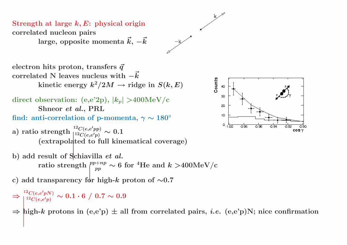
Strength at large k,E: physical origin
correlated nucleon pairs
large, opposite momenta ~k, −~k
electron hits proton, transfers ~q
correlated N leaves nucleus with −~k
kinetic energy k2/2M → ridge in S(k,E)
direct observation: (e,e’2p), |kp| >400MeV/c
Shneor et al., PRL
find: anti-correlation of p-momenta, γ ∼ 180
a) ratio strength12C(e,e′pp)12C(e,e′p)
∼ 0.1
(extrapolated to full kinematical coverage)
b) add result of Schiavilla et al.
ratio strength pp+nppp
∼ 6 for 4He and k >400MeV/c
c) add transparency for high-k proton of ∼0.7
⇒12C(e,e′pN)12C(e,e′p)
∼ 0.1 · 6 / 0.7 ∼ 0.9
⇒ high-k protons in (e,e’p) ± all from correlated pairs, i.e. (e,e’p)N; nice confirmation
Basic insight: need S(k,E) to describe nuclei
n(k) not sufficient!
Example: role of interaction in DIS
use only momentum distribution
parton distribution functions
i.e. ignore energy of initial state parton
also ignore final-state interaction of recoiling parton
Importance of interaction:
binding in case of DIS must be important
nuclear binding explains EMC-effect!
E for correlated N much larger than EMF
final state interaction plays role
claimed erroneously to disappear for Q2 = ∞
Brodsky et al. show that this is wrong
→ response functions are not distribution functions
will need to be improved upon
what is spectral function of quarks in nucleons?
Orthogonal look:
where correlated strength in r-space?
motivation: difficulties with QP-R(r)
• QP radial wave functions fitted to ρ(r)
poorly explain F(q) of QP-dominated transitions
• QP wave functions poorly explain ρ(r) at small r
reason: ρ(r) contains correlated contribution
presumably correlated radial shape 6= QP shape
⇒ question: radial distribution of correlated strength = ?
Two opposing tendencies:
• large E pulls correlated strength to small r
• higher (angular) momenta tend to shift it to larger r
which wins?
2 independent answers:
• study via selfconsistent Green’s function theory SGFT
H. Muther
• determine from (e,e) and (e,e′p)
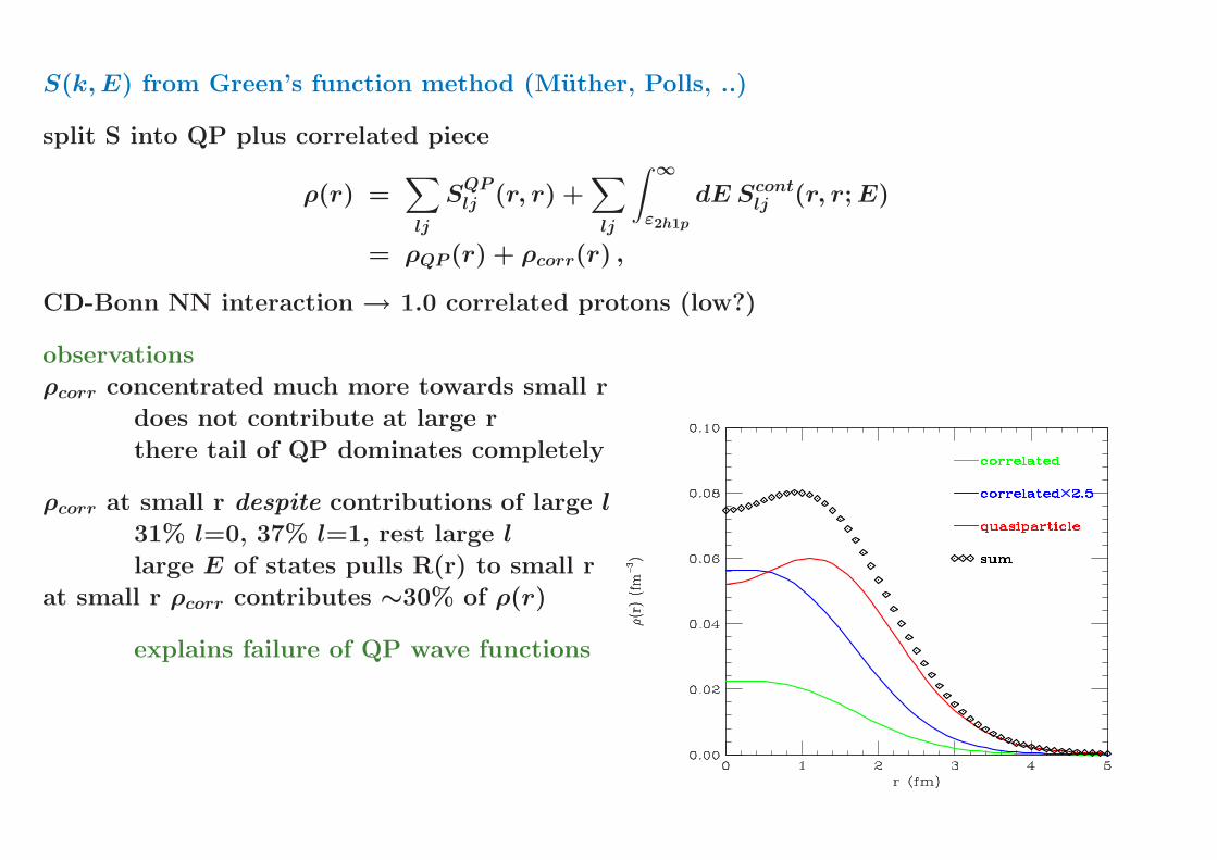
S(k,E) from Green’s function method (Muther, Polls, ..)
split S into QP plus correlated piece
ρ(r) =∑
lj
SQPlj (r, r) +∑
lj
∫ ∞
ε2h1p
dE Scontlj (r, r;E)
= ρQP (r) + ρcorr(r) ,
CD-Bonn NN interaction → 1.0 correlated protons (low?)
observations
ρcorr concentrated much more towards small r
does not contribute at large r
there tail of QP dominates completely
ρcorr at small r despite contributions of large l
31% l=0, 37% l=1, rest large l
large E of states pulls R(r) to small r
at small r ρcorr contributes ∼30% of ρ(r)
explains failure of QP wave functions
ρcorr from (e,e)+(e,e′p) data
ρcorr(r) = ρ(r)point −∑
QP−orbits
FBT (RQP (k))2
point density of C
have very precise (e,e) data up to large q
have µ-X-ray data
do modelindependent analysis (SOG)
→ charge density with small δρ
unfold nucleon size to get point density
QP wave functions from (e,e′p)
extensive set of (e,e′p) data
• low-q from NIKHEF, Saclay
analyzed with DWBA
optical potentials from (p,p)
• high-q data from SLAC, JLAB
analyzed with theoretical transparencies
confirmed by data
compilation: L. Lapikas et al., PRC61, 64325
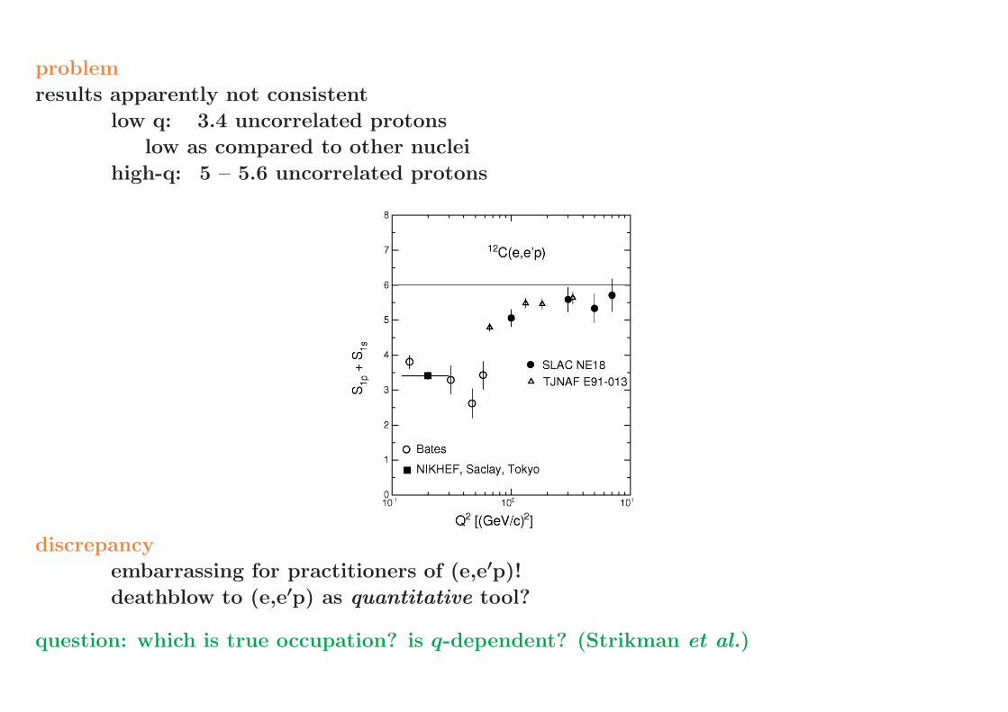
problem
results apparently not consistent
low q: 3.4 uncorrelated protons
low as compared to other nuclei
high-q: 5 – 5.6 uncorrelated protons
discrepancy
embarrassing for practitioners of (e,e′p)!
deathblow to (e,e′p) as quantitative tool?
question: which is true occupation? is q-dependent? (Strikman et al.)
issues: quality optical potentials, role MEC’s,
coupled-channel effects, value of T
one reason for difference obvious: sloppy interpretation
low-q data:
E ≤ 50MeV , k ≤ 180MeV/c
high-q data:
E ≤ 80MeV , k ≤ 300MeV/c
integrate over part of correlated strength, must remove before comparing!
correction of high-q result
use analysis of QP region of Rohe et al.
agrees with previous SLAC/JLAB data, uses most reliable T
calculate correlated contribution using theory, remove
result:
high-q: 4.5 uncorrelated protons
low-q: 3.4 uncorrelated protons
⇒ discrepancy much reduced
but: still larger than desirable, larger than believed ±10%
my choice: (corrected) high-q result
low-q for 12C anomalously low
(remember figure occupations)
low-q have significant MEC effects
Boffi: up to 20%
low-q would imply unrealistic correlated strength
would disagree with Rohe et al.
use high-q result
choice confirmed by consistency check, see below
further adjustment needed
1s fitted to data E < 50MeV
this region contains already some correlated strength
R(k)corr falls less quickly than R(k)QPmust correct shape of Lapikas R(k)1s
correction of shape:
• can do using QP and correlated S(k,E) from theory
• can analyze Rohe data with QP+correlated parts
find same result:
R(k) compressed by 11%
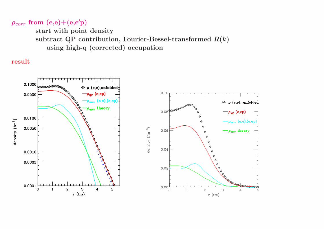
ρcorr from (e,e)+(e,e′p)
start with point density
subtract QP contribution, Fourier-Bessel-transformed R(k)
using high-q (corrected) occupation
result

observations
ρcorr concentrated towards small r
as was seen in theory
ρcorr gives ∼30% contribution at small r
explains failure of QP models
reasonable agreement with theory
(uncertainty of ρcorr ∼20%)
in exp. density perhaps more l > 1 strength
important consistency check: large r
perfect agreement ρQP ... ρpointshould occur as ρcorr cannot contribute
large-r = the region where MF ± OK
conclusions of r-space study
shape of ρcorr differs strongly from shape of ρQP
ρcorr gives 30% contribution in nuclear interior
explains failure of QP models, cannot be ’compensated’ using eeff , etc.
reasonable agreement with Green’s function theory
Conclusions
have finally data on correlated strength
... some 15 years after CBF calculation
± agrees with modern many-body theories
... which were amazingly good!
for quantitative understanding of nuclei:
must go beyond mean-field, include correlated nucleons
for good S(k,E) of finite nuclei
look forward to results from Fermi Hypernetted Chain calculations


