Periodicals of Engineering and Natural Sciences ISSN 2303-4521
Vol.6, No.1, June 2018, pp. 332~347
Available online at: http://pen.ius.edu.ba
DOI: 10.21533/pen.v6i1.275 332
Optimal and Efficient Time Series Classification with Burrows-
Wheeler Transform and Spectral Window Based Transformation
T. Karthikeyan 1, T. Sitamahalakshmi
2,
1 Departement of Electrical and Computer Engineering, Knowledge Institute of Technology, Salem, Tamilnadu, India. 2 Department of Computer Science and Engineering, GITAM University, Visakhapatnam, Andhra Pradesh, India.
Article Info ABSTRACT
Article history:
Received Dec 12th, 2017
Revised May 20th, 2018
Accepted Jun 7th, 2018
With the progressing amount of data every day, Time series classification acts
as a vital role in the real life environment. Raised data volume for the time
periods will make hard for the researchers to examine as well as assess the
data. Therefore time series classification is taken as a significant research
problem for the examining as well as identifying the time series dataset. On
the other hand the previous research might carry out low in case of existence
of weak classifiers. It is solved by introducing the Weak Classifier aware
Time Series Data Classification Algorithm (WCTSD). In this proposed
technique, with the help of the Burrows-Wheeler Transform (BWT), primarily
frequency domain based data transformation is carried out. After that, by
means of presenting the technique called spectral window based
transformation, time series based data transformation is performed. With the
help of the Hybrid K Nearest Neighbour, Hybrid decision tree algorithm,
Linear Multiclass Support Vector Machine, these transformed data is
classified. Here, to enhance the classification accuracy, the weak classifier is
eliminated by utilizing hybrid particle swarm with firefly algorithm. In the
MATLAB simulation environment, the total implementation of the presented
research technique is carried out and it is confirmed that the presented
research technique WCTSD results in providing the best possible outcome
compared to the previous research methods.
Keyword:
Time series classification, Burrows-Wheeler Transform, spectral window based
transformation, firefly algorithm, weak classifier,
Corresponding Author:
Third Author,
Departement of Electrical and Computer Engineering,
National Chung Cheng University,
168 University Road, Minhsiung Township, Chiayi County 62102, Taiwan, ROC.
Email: [email protected]
1. Introduction
Time series data is omnipresent [1]. Human activities as well as nature generates time series (data)
day by day and all over the place, such as financial recordings, weather readings, industrial observations and
physiological signals [2]. Since the modest kind of time series data, univariate time series offers a sensibly
good starting point to analyze these temporal signals [3]. The representation learning as well as classification
research has identified numerous possible applications in the areas such as industry, finance, and health care.
On the other hand, learning representations as well as classifying time series are even now fascinating more
consideration [4]. Since the earliest baseline, distance-based approaches work openly on raw time series with
certain pre-defined similarity measures for instance Euclidean distance or Dynamic time warping (DTW) to
T. Karthikeyan et al. PEN Vol. 6, No. 1, 2018, pp. 332 – 347
333
do classification [5]. The grouping of DTW as well as the k-nearest neighbor’s classifier is an effective
method as a golden standard in the last epoch [6].
The issue of time-series clustering as well as classification has been stated by means of describing a
distance metric amid time series, which includes matching up the sequential values directly [7]. By means of
utilizing a wide database of algorithms for computing thousands of diverse time-series properties, outcomes
prove that common feature based representations of time series could be utilized to handle classification
problems in time-series data mining. The method is obviously significant for numerous applications crosswise
the quantitative sciences where unprecedented volumes of data are being produced as well as maintained, and
as well for applications in industry (for instance categorizing irregularities on a production line), finance (for
example characterizing share price fluctuations), business (for instance identifying fake credit card
transactions), surveillance (for instance examining numerous sensor recordings), and medicine (for example
diagnosing heart beat recordings)[8].
Two foremost difficulties of time-series classification are: (i) choosing a suitable depiction of the time
series, and (ii) choosing an appropriate measure of dissimilarity or distance amid time series. The literature on
depictions as well as distance measures for time-series clustering and classification is broad [9]. Possibly the
most forth right depiction of a time series is its time-domain form, afterwards distances amid time series
associate with dissimilarities among the time-ordered measurements themselves [10]. While short time series
encode significant patterns, which must be matched up, novel time series could be categorized by comparing
them to identical instances of time series with a known classification [11].
This kind of problem has conventionally been the attention of the time series data mining community,
and we denote this method as instance-based classification [12]. An alternate method comprises signifying
time series utilizing a collection of derived properties, or features, and by this means transmuting the temporal
issue to a static one. An extremely simple example encompasses signifying a time series utilizing simply its
mean and variance, by this means transmuting time-series objects of any length into short vectors, which
includes these two properties [13]. Here we present an automated technique for creating these feature-based
representations of time series utilizing a huge database of time-series features. Not all approaches fit precisely
into these two types of instance-based as well as feature-based classification. E.g., time-series shapelet
categorize novel time series in keeping with the least distance of specific time-series subsequences (or
‘shapelet’) to that time series. Even if this technique utilizes distances computed in the time-domain as a
foundation for classification (not features), novel time series don’t want to be matched up with a huge amount
of training instances (as in instance-based classification).
By means of presenting the Weak Classifier aware Time Series Data Classification Algorithm
(WCTSD), this problem is solved in the presented research, in which, by means of presenting the Burrows-
Wheeler Transform (BWT), primarily frequency domain based data transformation is carried out. After that,
with the help of spectral window based transformation, time series based data transformation is carried out.
Afterwards, by means of the Hybrid K Nearest Neighbour, Hybrid decision tree algorithm, Linear Multiclass
Support Vector Machine, these transformed data is categorized. Here the weak classifier is eliminated to
enhance the classification accuracy by means of utilizing hybrid particle swarm with firefly algorithm.
2. Related works
Taktak et al [14]proposed a guesstimate of derivative, which needs merely one recursive computation
of the longest common subsequence (LCSS) (dis)similarity measure to attain 1 Nearest Neighbour(1NN)
classification with ideal memory requirement. Therefore, we present a set of advanced Symbolic Aggregate
approXimation (SAX) representation with LCSS amid compressed series of symbols. By means of using
T. Karthikeyan et al. PEN Vol. 6, No. 1, 2018, pp. 332 – 347
334
Piecewise Linear Regression, Advanced SAX focuses on including symbolic trend info. Gong et al [15]
presented a multiobjective learning technique for time series approximation as well as classification, named
MultiObjective Model-Metric (MOMM) learning in which a recurrent network is used as the temporal filter,
dependent upon which, a generative model is learned for every time series as a depiction of that series.
Hamdi et al [16] taken out time series samples of these Active Region parameters and propose a flare
prediction technique dependent upon the k-NN classification of the univariate time series. It is identified that,
for classification task, by utilizing a statistical summarization on the time series of a single Active Region
parameter, known as over-all unsigned current helicity, outdoes the usage of all Active Region parameters at a
single instant of time.
Li & Lin [17] presented a parameter-free time series classification technique, which contains a linear
time complexity. The method is assessed on the entire 85 datasets in the well-known University of California,
Riverside (UCR) time series classification archive. The outcomes prove that the novel technique attains
improved total classification accurateness performance compared to the extensively utilized benchmark.
Hong & Yoon [18] used the Internet-of-things (IoT) sensors for accurate as well as adequate data collection
and a hybrid of Deep Belief Network (DBN) and Long Short-Term Memory (LSTM) was presented for
precise sleep patterns classification.
Tamura &Ichimura [19] presented novel depiction for the time series classification using the
recurrence plot method. Moving Average Convergence Divergence (MACD) histogram is the speeding up of
time, which denotes the features of time series. So, the research technique is dependent upon MACD
histogram. Especially, a recurrence plot made from MACD histogram is known as a MACD-Histogram-based
recurrence plot (MHRP).
Karim et al [20] presented the augmentation of completely convolutional networks with Long Short
Term Memory Recurrent Neural Network (LSTM RNN) sub-modules for time series classification. The
presented models considerably improve the performance of completely convolutional networks with an
insignificant rise in model size as well as need minimal preprocessing of the data set.
Ye et al [21] presented a shape based similarity measure. By means of presenting a shape coefficient
into the traditional weighted dynamic time warping algorithm, an improved version, Shape based Weighted
Dynamic Time Warping (SWDTW) algorithm is introduced. Precisely, the means to compute univariate as
well as multivariate time series similarity with SWDTW are provided. Therefore time series classification
regarded to be more significant research problem for examining as well as identifying the time series dataset.
On the other hand the previous research might do low in case of existence of weak classifiers.
3. Optimal and efficient time series classification
In this presented technique, primarily frequency domain based data transformation is carried out by
means of presenting the Burrows-Wheeler Transform (BWT). Afterwards, by means of presenting the
technique called spectral window based transformation, time series based data transformation is carried out.
With the help of the Hybrid K Nearest Neighbour, Hybrid decision tree algorithm, Linear Multiclass Support
Vector Machine, these transformed data is categorized. Here, to improve the classification accuracy, the weak
classifier is eliminated by utilizing hybrid particle swarm with firefly algorithm.
3.1. Burrows-wheeler transform (BWT) for frequency domain
T. Karthikeyan et al. PEN Vol. 6, No. 1, 2018, pp. 332 – 347
335
In this research, to do the frequency domain analysis, Burrows-Wheeler Transform (BWT) is
presented [22].The BWT considers a block of data as well as reorganizes it with the help of a sorting
algorithm. The ensuing output block encompasses precisely the alike data elements that it initiated with,
opposing only in their ordering. The transformation is adjustable; signifying the real ordering of the data
elements could be reinstated without any loss of fidelity. The BWT is carried out on a whole block of data
simultaneously. Numerous today's famous lossless compression algorithms work in streaming mode, reading a
single byte or a small number of bytes all at once. On the other hand with this novel transform, we must work
on the biggest chunks of data possible. The Burrows-Wheeler Transform (BWT) does a permutation of the
characters in the text, with the intension that characters with identical lexical contexts in the text would be
clustered together. Consider T = t1t2 ...tn be the input text, where every character ti,1 ≤ i ≤ n is taken from a
finite ordered alphabet Σ. The forward BWT is carried out in the following steps:
1) Regularly rotate T to build n permutations of T. The permutations create a n × n matrix MM’, with
every row in MM’ signifying one permutation of T;
2) Sort the rows of MM’ lexicographically to create another matrix MM. MM (and MM’) comprises T
as one among its rows;
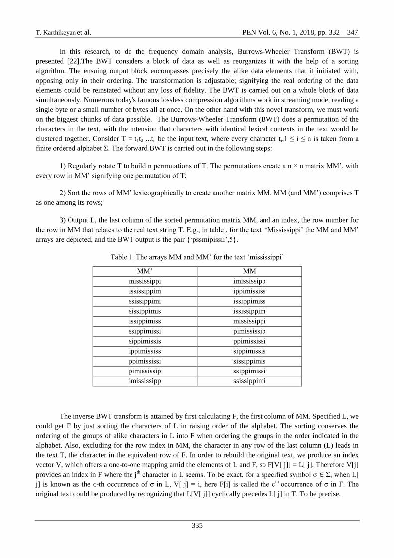
3) Output L, the last column of the sorted permutation matrix MM, and an index, the row number for
the row in MM that relates to the real text string T. E.g., in table , for the text ‘Mississippi’ the MM and MM’
arrays are depicted, and the BWT output is the pair {‘pssmipissii’,5}.
Table 1. The arrays MM and MM’ for the text ‘mississippi’
MM’ MM
mississippi imississipp
ississippim ippimississ
ssissippimi issippimiss
sissippimis ississippim
issippimiss mississippi
ssippimissi pimississip
sippimissis ppimississi
ippimississ sippimissis
ppimississi sissippimis
pimississip ssippimissi
imississipp ssissippimi
The inverse BWT transform is attained by first calculating F, the first column of MM. Specified L, we
could get F by just sorting the characters of L in raising order of the alphabet. The sorting conserves the
ordering of the groups of alike characters in L into F when ordering the groups in the order indicated in the
alphabet. Also, excluding for the row index in MM, the character in any row of the last column (L) leads in
the text T, the character in the equivalent row of F. In order to rebuild the original text, we produce an index
vector V, which offers a one-to-one mapping amid the elements of L and F, so F[V[ j]] = L[ j]. Therefore V[j]
provides an index in F where the jth character in L seems. To be exact, for a specified symbol σ ∈ Σ, when L[
j] is known as the c-th occurrence of σ in L, V[ j] = i, here F[i] is called the cth occurrence of σ in F. The
original text could be produced by recognizing that L[V[ j]] cyclically precedes L[ j] in T. To be precise,

T. Karthikeyan et al. PEN Vol. 6, No. 1, 2018, pp. 332 – 347
336
(1)
Here V1 [index] = index; and V
i+1 [s] = V[V
i [s]],1 ≤ s ≤ n. The seminal BWT gives an algorithm to do the
inverse BWT operation in linear time by creating an initial pass through the encoded string counting
characters.
3.2. Spectral window based transformation methods for time domain
A simple but effective switching framework is proposed that can alternate between both tools after
analyzing the input signal using spectrum sensing techniques. The first step involves spectrum sensing that
determines the orientation of the signal on the spectrum using the normalized power spectral density . The
expectation and standard deviation is extracted from as
(2)
(3)
where Ai is the amplitude of normalized Power Spectral Density (PSD) . The expectation returns
the frequency where PSD is concentrated. Together with , both give information about the distribution of the
PSD. A signal would be considered narrow band when is smaller than a user defined threshold . An
optimum threshold can be selected empirically such that smearing effect is minimized. After the analysis of
known narrow and wide-band signals, the value of is set to be 1500. The signals having less than 1500 are
considered as narrow band signal and the appropriate tool; that is, STFT is selected. As mentioned earlier,
Short Time Fourier Transform (STFT) is computationally less expensive and the smearing effect is not
prominent in case of narrow band signals. Signals having greater than 1500 are considered wide-band
signal. In such scenario, the proposed method will adopt Constant Q Transform (CQT) tool. Unlike the STFT,
CQT will minimize the smearing effect for wideband signal and improve the visualization of spectrogram.
The check will result in the selection of either the STFT or the CQT method as
(4)
Upon selection of STFT, the next step is to select an appropriate window size, where two closest
sinusoids can be distinguished. However, non-stationary signals may involve a large number of sinusoids in
close proximity. This results in a very small Δ and consequently a large window. This makes the STFT very
similar to the Fourier transform and will hamper temporal resolution. In order to select an appropriate window
size a novel empirical model is proposed that adaptively selects a window size by
(5)
Equation (5) will adopt an appropriate window size which does not lose any temporal information
after the transform, where the size of the main lobe of the window can be set to 2 for a rectangular, 4 for a
Hamming/Hanning, and 6 for a Blackman window. In this work, Hamming window is used and the value of
is set as 4.
3.3. Classification of time series data
In this section classifiers used for the time series data classification is discussed

T. Karthikeyan et al. PEN Vol. 6, No. 1, 2018, pp. 332 – 347
337
3.3.1. Hybrid K nearest Neighbour
In this work Fuzzy Relative transformation based K-local Hyper plane distance Nearest Neighbor
(FRHKNN) classifier is introduced to tackle the noises present in the input features. FRHKNN first generates
the balance training set to tackle the unbalance problem. Then, the relative transformation is adopted by
FRHKNN to avoid the effect of noisy data. In the following, FRHKNN constructs the local hyperplane and
calculates the local hyperplane distance for each class. Finally, the fuzzy membership function is used to
summarize the local hyperplane distance and predicts the label of the query vector. Specifically, assume that:
1) v is a query feature vector; 2) F = {f1, f2,..., fn} is the set of training feature vectors (where n is the number
of training feature vectors), and Y = {y1, y2,..., yn} is the corresponding set of the labels with respect to F
(where yi∈ {1, 2,..., k}, i ∈ {1,..., n}); 3) each class is denoted as Cj ( j ∈ {1,..., k}), and the number of feature
vectors in each class Cj is represented by nj; 4) ε is the size of the neighborhood in the classification process
(where ε is an integer); and 5) β is the penalty parameter for classification. In the first step, FRHKNN first
constructs a local environment for the query feature vector v, which is defined as ε nearest neighbors of the
query feature vector v in each class Cj based on the Euclidean distance, and generates a new balance training
set Fas follows
F = ∪jFj(ε, v) (6)
Fj(ε, v) = {fi∈Cj | φ(fi, v) ≤ φεj} (7)
where φ denotes the Euclidean distance function, and φεj denotes the Euclidean distance between the
query vector v and the ε nearest neighbor in the class Cj. The local environment enables FRHKNN to avoid
the effect of the unbalanced problem. And the balance training set treats all the classes equally, which is able
to avoid the class boundary biased in favor of the class with more feature vectors.
3.3.2. Hybrid decision tree algorithm
In this segment, we define the foremost characteristics of technique for managing with the issue of
small disjuncts. This is a hybrid technique, which unites decision trees as well as genetic algorithms. The
fundamental notion is to utilize a decision tree algorithm to categorize examples be the property of huge
disjuncts and utilize a genetic algorithm to find out rules categorizing examples be a member of small
disjuncts. The technique finds rules in two training phases. In the primary stage, it runs C4.5, a famous
decision tree induction algorithm. The persuaded, pruned tree is transmuted into a collection of rules. This rule
set is considered as stated in disjunctive normal form, with the intension that every rule relates to a disjunct.
Every rule is taken as a small disjunct or as a ‘‘large’’ (non-small) disjunct, based upon whether or not its
coverage (the no of examples covered by the rule) is lesser than or equivalent to a specified threshold. The
second phase utilizing a genetic algorithm to find out rules covering the examples be a member of small
disjuncts. If not––that is to say the leaf node is a small disjunct––the example is allotted the class of one
among the small-disjunct rules found by the GA.
3.3.3. Linear Multiclass Support Vector Machine
The multi-class SVM with the linear kernel is introduced in keeping with the selected feature. Instead
of creating numerous binary classifiers, a proper way is to examine complete classes in a single optimization
processing. For a k-class problem, these techniques design an individual objective function for directing
complete k-binary SVMs all at once and prolong the margins from each class to the remaining classes. Given
with a labeled training set represented by of cardinality l, here ∈ and ∈
, the formulation is provided in this manner:

T. Karthikeyan et al. PEN Vol. 6, No. 1, 2018, pp. 332 – 347
338
∈ ∈ ∈
(8)
Cause to undergo
(9)
, ∈ (10)
The resultant decision function is
(11)
As the kernel matrix would be positive as well as semi-definite, their product helps in enhancing the
accurateness of classification. Consequently, the single variant time series data could be efficiently
categorized with the help of the presented Multi-class SVM.
3.4. Weak classifier removal using cross validation
In the present research, so as to enhance the TSC performance through ensembling, ensemble
classifier is presented. Even if the value of ensembling is known, former method is rare in that we add
diversity by accepting a heterogeneous ensemble instead of utilizing resampling techniques with weak
learners. Owing to weak learners in the classification model they contain certain drawbacks
The complete accuracy of the complete time series classification system would reduce.
Albeit the accuracy of the classifier is decreased it needs extra time to confirm the classification
system, to improve accuracy.
The weaker learners is confirmed by utilizing numerous statistical test functions with numerous
number of iteration, on the other hand still to attain improved performance for weaker learners turn out to be
insoluble. With the intension of resolving the aforesaid problems in this proposed method provides a novel
classifier or presents an efficient cross validation schema, which compute the precision of the classifier with
the error value of the system that eliminates the weaker learners during training phase. This improves the
outcomes of the classifiers as well as enhances the execution time of the heterogeneous classification
ensemble schema or classifiers to time series dataset samples. In this research, with the help of the Hybrid
Particle Swarm Optimization with FireFly Algorithm (PSO-FFA), weak classifier removal is carried out.
The presented PSO-FFA is a technique of uniting the benefits of quicker computation of Particle
Swarm Optimization with sturdiness of FFA with the intention of improving the global search ability. The
PSO algorithm begins with a collection of solutions and dependent on the survival of fittest principle, merely
the finest solution moves from one phase two other. This process is recurrent till any of the convergence
conditions is attained. Finally, the ideal solution is the one with the least total cost out of the collection of
solutions. The time of convergence of PSO based on the values of the arbitrarily set control parameters. FFA

T. Karthikeyan et al. PEN Vol. 6, No. 1, 2018, pp. 332 – 347
339
algorithm begins with a primary operating solution and till the convergence criteria is attained, each iteration
enhances the solution. The ideal solution attained from FFA algorithm based on the quality of the primary
solution presented. The initial solution given to FFA is the best possible solution got from PSO algorithm. So,
the best possible solution attained from this Hybrid approach is superior to the solution got from PSO or FFA
algorithms. A portion of PSO is utilized in the FFA to improve convergence and as well to improve its ability
for not fall into the local minimum. The PSO-FFA has precisely the similar steps as the FFA with the
exclusion that the position vector of FFA is changed in this manner: In the PSO-FFA, the distance amid xi and
pbesti , is the Cartesian distance
(12)
The distance amid xi and gbesti, is the Cartesian distance
(13)
The position vectors xi of the FFPSO is arbitrarily mutated by means of utilizing Eq. (14)
(14)
Here acceleration coefficients for personal best as well as global best, w be the property of
inertia weight, randomization value.
Procedure of PSO-FFA
1. Generate the initial population randomly.
2. Initialize pbest and gbest.
3. Calculate the fitness of initial population based on light intensity of fireflies.
4. While (stopping criteria is satisfied)
5. For i=1:p ( p fireflies)
6. For j=1:p
6.1. Light intensity I is determined classification accuracy
6.2. Distance between pbest-xi and gbest-xi is calculated using eqs. (12) and (13).
6.3. If (I(i)<I(j))
Firefly i is moved towards firefly j using eq. (14)
6.4. Else
Firefly i is moved randomly towards firefly j using eq (14)
6.5. End If
7. Calculate the new solutions and update the light intensity value
8. Update pbest and gbest.
9. End for j
10. End for i
11. Sort the fireflies in descending order based on their light intensity
12. End while

T. Karthikeyan et al. PEN Vol. 6, No. 1, 2018, pp. 332 – 347
340
In the recommended method, the light intensity attraction step of every particle gets changed by a
PSO operator. Now, every particle is arbitrarily fascinated in the direction of the gbest position in the
complete population. Local search in diverse areas is carried by the altered attraction step of the PSO-FFA
algorithm. The foremost goal of PSO-FFA feature selection phase is to decrease the features of the issue
beforehand the supervised neural network classification. Amongst all the wrapper algorithms utilized, PSO-
FFA that resolves optimization problems utilizing the approaches of flashing behavior of fireflies, has
progressed as a hopeful one.
4. Results and discussion
The performance of the presented Weak Classifier aware Time Series Data Classification Algorithm
(WCTSD) is assessed as well as matched up in this segment. ECG 200 & ECG 5000 dataset is used for the
evaluation. In MATLAB, the assessments are carried out with the performance parameters called specificity,
sensitivity, recall, precision, g-mean,f-measure and accuracy. The assessment is done amid the approaches
called SVM, KNN and hybrid Decision Tree algorithm for the changing amount of input samples.
The ECG200 dataset contains 200 ECG signals, all contains 96 measured values (every time series
reproduces 1 heartbeat). The dataset is categorized as 100 training signals as well as 100 testing signals.
Amongst 200 time series, 133 were termed as normal when the remaining 67 are termed as abnormal. Time
series are segments of a long ECG signal; subsequently the experimentations on this dataset mimic the
situation while the automatic recognition system is preferred to hold the doctor when she or he is searching
irregular portions of a long ECG signal. The real dataset for "ECG5000" is downloaded from Physionet,
which is a 20-hour long ECG. The name is BIDMC Congestive Heart Failure Database (CHFDB) and it is
record "chf07". It pre-processed the data by the following two steps: (1) Drew-out each heartbeat, (2) produce
each heartbeat of equivalent length by using the interpolation. This dataset is used in paper" A common
framework for never-ending learning from time series streams", DAMI 29(6). Afterward,5,000 heartbeats are
selected arbitrarily and utilize this ECG5000 with 5 classes. The dataset is separated into 500 training signals
as well as 4500 testing signals.
Precision and recall
Precision is the positive predictive value (PPV) and Recall is the true positive rate or sensitivity, [23-24]
(15)
(16)
Specificity (alias true negative rate) computes the ratio of real negatives, which are appropriately
identified as such (for instance the ratio of healthy people appropriately found as not containing the
condition).
(17)
T. Karthikeyan et al. PEN Vol. 6, No. 1, 2018, pp. 332 – 347
341
F-measure
The weighted harmonic mean of precision and recall [24]
(18)
G-mean
It is the geometric mean. For vectors, geomean(x) is known as the geometric mean of the elements in
x.
(19)
Accuracy
It is the whole precision of the model and is computed as the total actual classification parameters
( that is divided by the total of the classification parameters ( It is calculated like
this:
(20)
Evaluation made with former approaches for instance COTE, TSF, MSVM -KNN and presented
WCTSD classifier is depicted in the figures and conversed details dependent upon their performance measure
values. In the table 1, the numerical values attained for these methods are depicted.
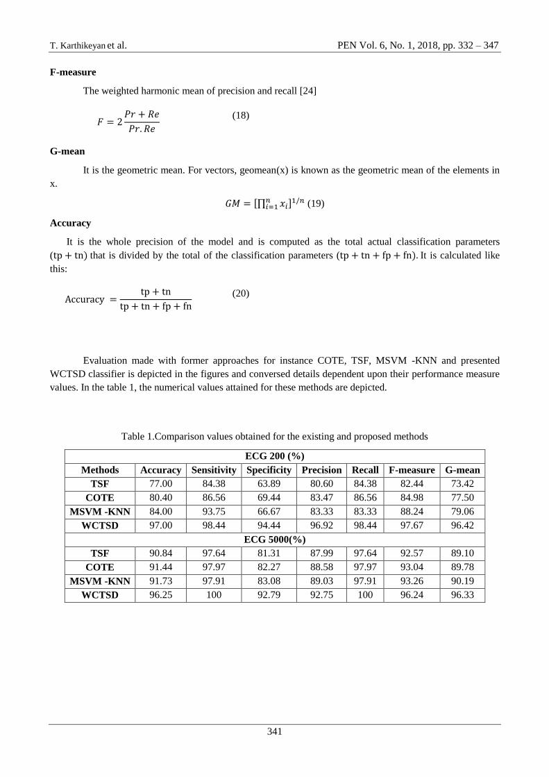
Table 1.Comparison values obtained for the existing and proposed methods
ECG 200 (%)
Methods Accuracy Sensitivity Specificity Precision Recall F-measure G-mean
TSF 77.00 84.38 63.89 80.60 84.38 82.44 73.42
COTE 80.40 86.56 69.44 83.47 86.56 84.98 77.50
MSVM -KNN 84.00 93.75 66.67 83.33 83.33 88.24 79.06
WCTSD 97.00 98.44 94.44 96.92 98.44 97.67 96.42
ECG 5000(%)
TSF 90.84 97.64 81.31 87.99 97.64 92.57 89.10
COTE 91.44 97.97 82.27 88.58 97.97 93.04 89.78
MSVM -KNN 91.73 97.91 83.08 89.03 97.91 93.26 90.19
WCTSD 96.25 100 92.79 92.75 100 96.24 96.33
T. Karthikeyan et al. PEN Vol. 6, No. 1, 2018, pp. 332 – 347
342
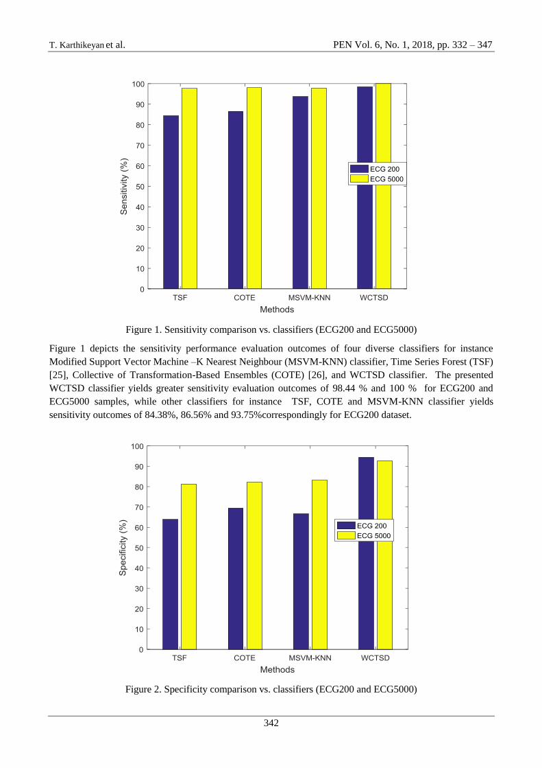
Figure 1. Sensitivity comparison vs. classifiers (ECG200 and ECG5000)
Figure 1 depicts the sensitivity performance evaluation outcomes of four diverse classifiers for instance
Modified Support Vector Machine –K Nearest Neighbour (MSVM-KNN) classifier, Time Series Forest (TSF)
[25], Collective of Transformation-Based Ensembles (COTE) [26], and WCTSD classifier. The presented
WCTSD classifier yields greater sensitivity evaluation outcomes of 98.44 % and 100 % for ECG200 and
ECG5000 samples, while other classifiers for instance TSF, COTE and MSVM-KNN classifier yields
sensitivity outcomes of 84.38%, 86.56% and 93.75%correspondingly for ECG200 dataset.
Figure 2. Specificity comparison vs. classifiers (ECG200 and ECG5000)

T. Karthikeyan et al. PEN Vol. 6, No. 1, 2018, pp. 332 – 347
343
Figure 2 depicts the specificity performance evaluation outcomes of four diverse classifiers for instance
COTE, TSF , MSVM-KNN classifier and WCTSD classifier. The presented WCTSD classifier yields greater
specificity outcomes of 94.44 % and 92.79 % for ECG200 and ECG5000 samples, while other classifiers for
instance TSF, COTE and MSVM-KNN classifier yields specificity outcomes of 63.89%, 69.44% and 66.67%
correspondingly for ECG200 dataset.
Figure 3. Precision comparison vs. classifiers(ECG200 and ECG5000)
Figure 3 depicts the precision evaluation outcomes of four diverse classifiers for instance TSF, COTE,
MSVM-KNN classifier and WCTSD classifier. The WCTSD classifier yields greater precision evaluation
outcomes of 96.92 % and 92.75 % for ECG200 and ECG5000 samples, while other classifiers for instance
TSF, COTE and MSVM-KNN classifier yields precision outcomes of 80.60%, 83.47% and 83.33%
correspondingly for ECG200 dataset.
Figure 4. Recall comparison vs. classifiers (ECG200 and ECG5000)

T. Karthikeyan et al. PEN Vol. 6, No. 1, 2018, pp. 332 – 347
344
Figure 4 depicts the recall outcomes of four different classifiers for instance TSF, COTE, MSVM-KNN
classifier and WCTSD classifier. The WCTSD classifier yields greater recall outcomes of 98.44 % and
100.00 % for ECG200 and ECG5000 samples, while other classifiers for instance TSF, COTE and MSVM-
KNN classifier yields recall outcomes of 84.38%, 86.56% and 83.33% correspondingly for ECG200 dataset.
Figure 5. F-measure comparison vs. classifiers(ECG200 and ECG5000)
Figure 5 depicts the f-measure outcomes of four diverse classifiers for instance TSF, COTE, MSVM-KNN
classifier and WCTSD classifier. The WCTSD classifier yields greater f-measure outcomes of 97.67 % and
96.24 % for ECG200 and ECG5000 samples, while other classifiers for instance TSF, COTE and MSVM-
KNN classifier yields f-measure outcomes of 82.44%, 84.98% and 88.24% correspondingly for ECG200
dataset.
Figure 6. G-mean comparison vs. classifiers(ECG200 and ECG5000)
T. Karthikeyan et al. PEN Vol. 6, No. 1, 2018, pp. 332 – 347
345
Figure 6 depicts the G-mean outcomes of four diverse classifiers for instance TSF, COTE, MSVM-KNN
classifier and WCTSD classifier. The WCTSD classifier yields greater G-mean comparison outcomes of
96.42 % and 96.33 % for ECG200 and ECG5000 samples, while other classifiers for instance TSF, COTE
and MSVM-KNN classifier yields G-mean outcomes of 73.42%, 77.5% and 79.06%correspondingly for
ECG200 dataset.
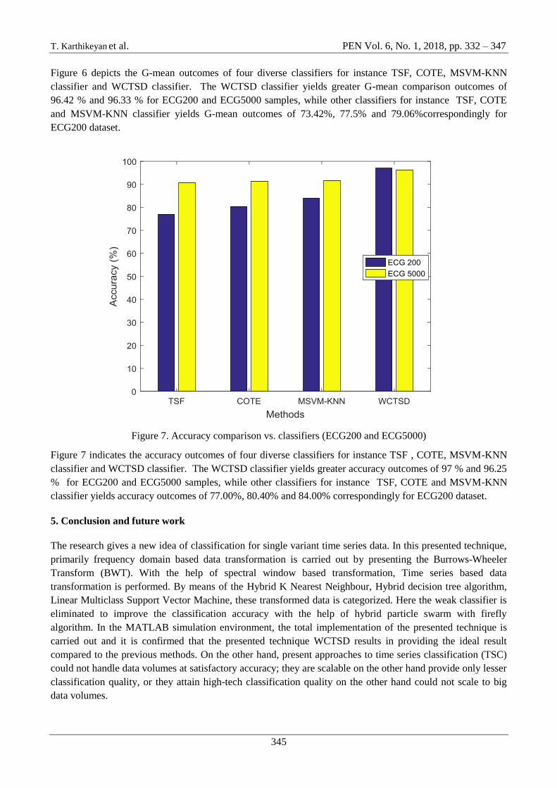
Figure 7. Accuracy comparison vs. classifiers (ECG200 and ECG5000)
Figure 7 indicates the accuracy outcomes of four diverse classifiers for instance TSF , COTE, MSVM-KNN
classifier and WCTSD classifier. The WCTSD classifier yields greater accuracy outcomes of 97 % and 96.25
% for ECG200 and ECG5000 samples, while other classifiers for instance TSF, COTE and MSVM-KNN
classifier yields accuracy outcomes of 77.00%, 80.40% and 84.00% correspondingly for ECG200 dataset.
5. Conclusion and future work
The research gives a new idea of classification for single variant time series data. In this presented technique,
primarily frequency domain based data transformation is carried out by presenting the Burrows-Wheeler
Transform (BWT). With the help of spectral window based transformation, Time series based data
transformation is performed. By means of the Hybrid K Nearest Neighbour, Hybrid decision tree algorithm,
Linear Multiclass Support Vector Machine, these transformed data is categorized. Here the weak classifier is
eliminated to improve the classification accuracy with the help of hybrid particle swarm with firefly
algorithm. In the MATLAB simulation environment, the total implementation of the presented technique is
carried out and it is confirmed that the presented technique WCTSD results in providing the ideal result
compared to the previous methods. On the other hand, present approaches to time series classification (TSC)
could not handle data volumes at satisfactory accuracy; they are scalable on the other hand provide only lesser
classification quality, or they attain high-tech classification quality on the other hand could not scale to big
data volumes.

T. Karthikeyan et al. PEN Vol. 6, No. 1, 2018, pp. 332 – 347
346
6. References
1. Cohen, M. X. (2014). Analyzing neural time series data: theory and practice.MIT press, pp.1-11.
2. Izakian, H., Pedrycz, W., & Jamal, I. (2015). Fuzzy clustering of time series data using dynamic time
warping distance. Engineering Applications of Artificial Intelligence, 39, 235-244.
3. Nazaripouya, H., Wang, B., Wang, Y., Chu, P., Pota, H. R., &Gadh, R. (2016). Univariate time series
prediction of solar power using a hybrid wavelet-ARMA-NARX prediction method. In Transmission and
Distribution Conference and Exposition (T&D), pp. 1-5.
4. Fulcher, B. D., & Jones, N. S. (2014). Highly comparative feature-based time-series classification. IEEE
Transactions on Knowledge and Data Engineering, 26(12), 3026-3037.
5. Fard, M.J., Pandya, A.K., Chinnam, R.B., Klein, M.D. and Ellis, R.D., 2017. Distance‐ based time series
classification approach for task recognition with application in surgical robot autonomy. The International
Journal of Medical Robotics and Computer Assisted Surgery, 13(3), p.e1766.
6. González, M., Bergmeir, C., Triguero, I., Rodríguez, Y., &Benítez, J. M. (2016). On the stopping criteria
for k-nearest neighbor in positive unlabeled time series classification problems. Information Sciences, 328,
42-59.
7. Aghabozorgi, S., Shirkhorshidi, A. S., &Wah, T. Y. (2015). Time-series clustering–A decade
review. Information Systems, 53, 16-38.
8. Yang, J., Nguyen, M. N., San, P. P., Li, X., &Krishnaswamy, S. (2015). Deep Convolutional Neural
Networks on Multichannel Time Series for Human Activity Recognition.In IJCAI , pp. 3995-4001.
9. Längkvist, M., Karlsson, L., &Loutfi, A. (2014). A review of unsupervised feature learning and deep
learning for time-series modeling. Pattern Recognition Letters, 42, 11-24.
10. Weigend, A. S. (2018). Time series prediction: forecasting the future and understanding the past.
Routledge.
11. Shokoohi-Yekta, M., Chen, Y., Campana, B., Hu, B., Zakaria, J., & Keogh, E. (2015, August). Discovery
of meaningful rules in time series.In Proceedings of the 21th ACM SIGKDD international conference on
knowledge discovery and data mining , pp. 1085-1094.
12. Salama, K. M., Abdelbar, A. M., Helal, A. M., &Freitas, A. A. (2017). Instance-based classification with
ant colony optimization. Intelligent Data Analysis, 21(4), 913-944.
13. Grzeszczuk, R., Chandrasekhar, V., Takacs, G., &Girod, B. (2017). U.S. Patent No. 9,710,492.
Washington, DC: U.S. Patent and Trademark Office.
14. Taktak, M., Triki, S., &Kamoun, A. (2017). SAX-based representation with longest common subsequence
dissimilarity measure for time series data classification. IEEE/ACS 14th International Conference on
In Computer Systems and Applications (AICCSA), pp. 821-828.
15. Gong, Z., Chen, H., Yuan, B. and Yao, X., 2018. Multiobjective Learning in the Model Space for Time
Series Classification. IEEE Transactions on Cybernetics, (99), pp.1-15.
16. Hamdi, S. M., Kempton, D., Ma, R., Boubrahimi, S. F., &Angryk, R. A. (2017). A time series
classification-based approach for solar flare prediction. IEEE International Conference onBig Data (Big
Data), pp. 2543-2551.
17. Li, X., & Lin, J. (2017). Linear Time Complexity Time Series Classification with Bag-of-Pattern-Features.
IEEE International Conference onData Mining (ICDM), pp. 277-286.
18. Hong, J., & Yoon, J. (2017). Multivariate time-series classification of sleep patterns using a hybrid deep
learning architecture. International Conference on e-Health Networking, Applications and Services
(Healthcom), pp. 1-6.
T. Karthikeyan et al. PEN Vol. 6, No. 1, 2018, pp. 332 – 347
347
19. Tamura, K., &Ichimura, T. (2017). MACD-histogram-based recurrence plot: A new representation for
time series classification. International Workshop on Computational Intelligence and Applications (IWCIA),
pp. 135-140.
20. Karim, F., Majumdar, S., Darabi, H., & Chen, S. (2018). LSTM fully convolutional networks for time
series classification. IEEE Access, 6, 1662-1669.
21. Ye, Y., Niu, C., Jiang, J., Ge, B., & Yang, K. (2017). A Shape Based Similarity Measure for Time Series
Classification with Weighted Dynamic Time Warping Algorithm. 4th International Conference on
Information Science and Control Engineering (ICISCE), pp. 104-109.
22. Burrows, M., & Wheeler, D. J. (1994). A block-sorting lossless data compression algorithm.
23. Sokolova, M. and Lapalme, G., 2009. A systematic analysis of performance measures for classification
tasks. Information Processing & Management, 45(4), pp.427-437.
24. García, S., Fernández, A., Luengo, J. and Herrera, F., 2009. A study of statistical techniques and
performance measures for genetics-based machine learning: accuracy and interpretability. Soft Computing,
13(10), pp.959-977.
25. Deng, H., Runger, G., Tuv, E. and Vladimir, M. A time series forest for classification and feature
extraction. Inf. Sci. 239 (2013) 142–153.
26. Bagnall, A., Lines, J., Hills, J. and Bostrom, A. Time-series classification with COTE: the collective of
transformation-based ensembles. IEEE Transactions on Knowledge and Data Engineering27(9) (2015) 2522-
2535.


