
I
Optimal design of a CO2 absorption unit and
assessment of solvent degradation
PhD Thesis
Mid-Term Report
June 2011
Grégoire Léonard

II

III
Table of content
1 INTRODUCTION ................................................................................................................. 1
1.1 CONTEXT OF THIS WORK .................................................................................................... 1
1.2 POST-COMBUSTION CO2 CAPTURE ..................................................................................... 1
2 OBJECTIVES ....................................................................................................................... 3
3 MODELING .......................................................................................................................... 4
3.1 EQUILIBRIUM MODEL ......................................................................................................... 4
3.2 RATE-BASED MODEL.......................................................................................................... 4
3.2.1 Advantages of the rate-based model ......................................................................... 4
3.2.2 Description of the rate-based model ......................................................................... 6
3.3 SIMULATION RESULTS ....................................................................................................... 8
3.3.1 Sensitivity study of process parameters .................................................................... 8
3.3.2 Model improvements ............................................................................................... 10
3.4 PERSPECTIVES ................................................................................................................. 14
4 DEGRADATION ................................................................................................................ 15
4.1 LITERATURE REVIEW ...................................................................................................... 16
4.1.1 Degradation mechanisms ........................................................................................ 16
4.1.2 Degradation products ............................................................................................. 16
4.1.3 Research groups ...................................................................................................... 17
4.2 DESCRIPTION OF THE DEGRADATION TEST RIG AT THE UNIVERSITY OF LIÈGE ............... 19
4.2.1 Degradation reactor ................................................................................................ 19
4.2.2 Gas supply system ................................................................................................... 20
4.2.3 Water balance control ............................................................................................. 21
4.2.4 Gas outlet ................................................................................................................ 21
4.2.5 Control Panel .......................................................................................................... 22
4.3 ANALYTICAL METHODS ................................................................................................... 22
4.3.1 High-Pressure Liquid Chromatography (HPLC) ................................................... 23
4.3.2 Gas Chromatography (GC) ..................................................................................... 28
4.3.3 Fourier Transformed Infra Red analysis (FTIR) .................................................... 30
4.3.4 Ion analysis ............................................................................................................. 33
4.3.5 Karl-Fischer titration of water ................................................................................ 33
4.4 RESULTS SUMMARY OF THE FIRST TESTS PERFORMED ...................................................... 34
4.4.1 Description of the experiments ................................................................................ 34

IV
4.4.2 Experimental feed-back ........................................................................................... 36
4.4.3 HPLC Quantification of MEA degradation ............................................................ 37
4.4.4 GC spectra of degraded MEA ................................................................................. 39
4.4.5 Ion analysis results .................................................................................................. 47
4.4.6 Karl-Fischer titration results .................................................................................. 48
5 CONCLUSION AND PERSPECTIVES ........................................................................... 50
6 BIBLIOGRAPHY ............................................................................................................... 51
7 ABBREVIATION LIST ..................................................................................................... 54
8 APPENDICES ..................................................................................................................... 55

V
Figure Index
Figure 1.1: Flowsheet of the chemical absorption process (IPCC, 2005) .................................. 1
Figure 3.1: Complexity levels while modeling the CO2 reactive absorption (Lawal et al.,
2008) ................................................................................................................................... 5
Figure 3.2: Representation of the gas-liquid interface ............................................................... 6
Figure 3.3: Influence of the solvent flow rate on the process energy requirement .................... 9
Figure 3.4 a and b : Influence of stripper pressure and solvent concentration on process energy
requirement ....................................................................................................................... 10
Figure 3.5: Process improvement on the CO2 capture flowsheet ............................................. 11
Figure 3.6: Influence of the intercooler location on the regeneration energy requirement ...... 12
Figure 3.7: Absorber temperature profiles for different intercooler locations ......................... 12
Figure 3.8: Determination of the optimal split flow return stage ............................................. 13
Figure 3.9: Optimization of the solvent flow rate in the split-flow configuration ................... 13
Figure 4.1 : Degradation products of MEA .............................................................................. 17
Figure 4.2: Flow sheet diagram of the Degradation Test Rig .................................................. 19
Figure 4.3: Reactor and hollow shaft agitator .......................................................................... 20
Figure 4.4: Description of the reactor head .............................................................................. 20
Figure 4.5: Bottle rack and gas supply ..................................................................................... 21
Figure 4.6: Water balance control (saturator and condenser) .................................................. 21
Figure 4.7: Connecting schema of the gas system ................................................................... 22
Figure 4.8: HPLC apparatus ..................................................................................................... 23
Figure 4.9: C18 Pyramid stationary phase ............................................................................... 24
Figure 4.10 : Nucleosil SA stationary phase ............................................................................ 24
Figure 4.11: HPLC calibration curve for MEA ........................................................................ 25
Figure 4.12: HPLC spectra of degraded MEA, Nucleosil SA column .................................... 26
Figure 4.13 : HILIC stationary phase ....................................................................................... 26
Figure 4.14: HPLC spectra of degraded MEA, Kinetex HILIC column .................................. 27
Figure 4.15: Gas chromatograph .............................................................................................. 28
Figure 4.16: GC spectrum of the main standards ..................................................................... 29
Figure 4.17: GC spectrum of MEA with internal standard ...................................................... 30
Figure 4.18 : FTIR analyser ..................................................................................................... 31
Figure 4.19: syringe pump and heated plate ............................................................................ 31
Figure 4.20: FTIR spectrum of a CO2-H2O sample ................................................................. 32

VI
Figure 4.21: FTIR spectrum of a MEA-H2O sample ............................................................... 32
Figure 4.22: FTIR spectrum of a NH3-H2O sample ................................................................. 33
Figure 4.23: Guide with PTFE bushing for the agitator support .............................................. 37
Figure 4.24: MEA concentrations measured during the degradation experiments .................. 38
Figure 4.25: GC spectrum of Experiment 1, final sample, diluted 1:10 .................................. 40
Figure 4.26 : GC spectrum of Experiment 2, final sample, diluted 1:10 ................................. 40
Figure 4.27 : GC spectrum of Experiment 3, final sample, diluted 1:10 ................................. 41
Figure 4.29 : GC spectrum of Experiment 5, final sample, diluted 1:10 ................................. 42
Figure 4.30 : GC spectrum of Experiment 6, final sample, diluted 1:10 ................................. 43
Figure 4.31 : GC spectrum of Experiment 7, final sample, diluted 1:10 ................................. 44
Figure 4.32 : GC spectrum of Experiment 8, final sample, diluted 1:10 ................................. 45
Figure 4.33 : GC spectrum of Experiment 9, final sample, diluted 1:10 ................................. 45
Figure 4.34 : GC spectrum of Experiment 10, final sample, diluted 1:10 ............................... 46
Figure 4.35: Results of the KF analysis and comparison with mass balance results ............... 49

VII
Table index
Table 1.1: Chemical reactions of CO2 absorption with MEA .................................................... 2
Table 3.1: Kinetics constants for the rate-based model ............................................................. 7
Table 3.2: Constants for the calculation of equilibrium constants ............................................. 7
Table 3.3: Rate-based model parameters ................................................................................... 7
Table 3.4: Optimization of process parameters ........................................................................ 10
Table 3.5: Comparison of different process improvements ..................................................... 14
Table 4.1: Literature review of recent MEA degradation studies ............................................ 18
Table 4.2: Characteristics of the C18 Pyramid HPLC column ................................................ 24
Table 4.3: Characteristics of the Nucleosil SA HPLC column ................................................ 25
Table 4.4 : Characteristics of the Kinetex HILIC HPLC column ............................................ 27
Table 4.5 : Characteristics of the OPTIMA-35 MS GC column .............................................. 28
Table 4.6: GC Characteristic of standard degradation products .............................................. 29
Table 4.7: Characteristic absorption wavelength for FTIR analysis ........................................ 32
Table 4.8: Analysis methods of ions ........................................................................................ 33
Table 4.9: Operating conditions of the degradation experiments ............................................ 35
Table 4.10: MEA concentration at the experiments’ end ......................................................... 38
Table 4.11: Main degradation products in Experiment 1 ......................................................... 40
Table 4.12: Main degradation products in Experiment 2 ......................................................... 40
Table 4.13: Main degradation products in Experiment 3 ......................................................... 41
Table 4.14: Main degradation products in Experiment 4 ......................................................... 42
Table 4.15: Main degradation products in Experiment 5 ......................................................... 42
Table 4.16: Main degradation products in Experiment 6 ......................................................... 43
Table 4.17: Main degradation products in Experiment 7 ......................................................... 44
Table 4.18: Main degradation products in Experiment 8 ......................................................... 45
Table 4.19: Main degradation products in Experiment 9 ......................................................... 45
Table 4.20: Main degradation products in Experiment 10 ....................................................... 46
Table 4.21: Degradation products in each experiment ............................................................. 46
Table 4.22: Evolution of ion concentrations in solution, in ppm ............................................. 47
Table 4.23: Results of the KF analysis and comparison with mass balance results ................ 48

1 Introduction
1
1 Introduction
1.1 Context of this work
Global climate change is a fact and the influence of human activity on this change through
greenhouse gases’ emission is widely recognized by the international scientific community.
The largest emitted greenhouse gas is CO2, and fossil fuel power plants are amongst the
largest CO2 emitters.
Regulatory frameworks, public opinions and scientific community all agree on the importance
of acting now to reduce CO2 emissions. The best way to do so is first to encourage energy
savings and reduce energy losses. Then, the development of renewable energies has to be
enhanced in order to become a large part of the future energy mix.
Many studies report that coal combustion will remain one of the largest power sources in the
next decades (among others, see the World Energy Outlook, 2010). Three main solutions can
contribute to the reduction of CO2 emissions in coal power plants: continuous improvement of
energy efficiency, which has already been performed to a large extent, biomass co-
combustion and carbon capture and storage.
In this framework, Carbon Capture and Storage (CCS) technologies for power plants are a
necessary technical development. They should perform the transition between our carbon-
based society with its greenhouse gases emissions concerns and a society based on sustainable
energy systems.
1.2 Post-combustion CO2 capture
This work focuses on the post-combustion capture process. It is based on the reactive
absorption of CO2 with an amine solvent, most commonly an aqueous solution of 30 wt-%
monoethanolamine (MEA, NH2-CH2-CH2-OH, C2H7NO). The principle of this process is
represented in figure 1.1.
Figure 1.1: Flowsheet of the chemical absorption process (IPCC, 2005)

1 Introduction
2
In the case of a coal power plant, the flue gas contains in volume approximately 14% CO2,
6% O2, 12% H2O and 68% N2. Some impurities (NOx, SOx, HCl, …) are still present in the
flue gas, so that different gas purification steps are necessary, like FGD (flue gas
desulfurization), SCR (selective catalytic reduction), and a wet pre-scrubbing treatment to
remove the remaining SO2 and achieve the desired temperature. After purification, the flue
gas enters the absorption column (also named “absorber”). Carbon dioxide is absorbed with a
chemical solvent at temperatures varying between 40 and 60°C depending on the solvent
(55°C in the case of MEA). The main reactions taking place during the absorption are listed in
table 1.1 for the MEA case.
Table 1.1: Chemical reactions of CO2 absorption with MEA
2 H2O <--> H3O+ + OH
-
C2H7NO + H3O+ <--> C2H8NO
+ + H2O
CO2 + 2 H2O <--> H3O+ + HCO3
-
HCO3- + H2O <--> H3O
+ + CO3
2-
C2H7NO + HCO3- <--> C3H6NO3
- + H2O
After CO2 absorption, the treated flue gas usually flows through a water-wash section and a
demister in which the entrained solvent droplets are separated from the gas. The CO2-loaded
solvent (also referred to as “rich solvent”) is pumped to a regeneration column (also named
“stripper”) via an heat-exchanger where the rich solvent is pre-heated.
In the stripper, the solvent is regenerated at temperatures varying between 100 and 140°C
(120°C in the case of MEA). The purpose of the reboiler at the stripper bottom is to supply
heat for the solvent regeneration. At this temperature, the absorption reaction is counter-
balanced by the desorption reaction, so that CO2 is released from the solvent. The regenerated
solvent (“lean solvent”) is fed back to the absorber via the rich-lean heat exchanger where it
gives its energy to pre-heat the rich solvent. A further heat exchanger cools the regenerated
solvent down to the right absorber entrance temperature.
The gaseous CO2 stream at the exit of the desorption column contains some water that is
removed in the condenser, so that the final product may reach a CO2-purity of 99% by
volume. The objective that is generally pursued in post-combustion processes is the removal
of 90% of the CO2 present in the power plant flue gas stream.

2 Objectives
3
2 Objectives
Based on a master thesis written in 2009, this PhD thesis in the field of chemical engineering
has been launched at the University of Liège in an industrial partnership with the company
Laborelec, part of the GDF SUEZ group.
The first sub-topics of this PhD thesis is the simulation and the optimization of the CO2 post-
combustion capture process with amines. The Aspen Plus® software (Advanced System for
Process Engineering) has been chosen as a performing simulation tool to simulate the CO2
capture process. Once the model is built, the first goal is to identify process parameters that
have the largest influence on the energy requirement of the CO2 capture, to study their
influence on the process, and to optimize them. This has already been performed based on a
sensitivity analysis for which results are presented in chapter 3. The second goal of the
simulation part is to dispose of a precise model that describes a pilot CO2 capture installation
for which Laborelec has been associated to the development. This model – the same that has
undergone the optimization procedure – should be validated using experimental data from the
pilot installation as soon as those will be available.
The second sub-topic of the thesis concerns the degradation of amine solvents used for CO2
capture. It is detailed in chapter 4. Since amine degradation is due to chemical reactions with
slow kinetics, a degradation test rig has been constructed at the University of Liège for the
experimental study of accelerated degradation under high pressure and high temperature
conditions. This equipment allows the study of amine degradation in batch mode as well as in
semi-batch mode, by which a gas continuously flows through the solvent solution. A
particular interest will be devoted to the degradation of MEA solutions, since MEA is the
most widely used amine for CO2 capture. However, some alternative solvents should also be
tested. The influence of different parameters (temperature, pressure, gas composition and
mass flow) on solvent degradation will be identified and quantified. Furthermore, since
corrosion and degradation inhibitors are commonly used in industrial processes, their impact
will be studied as well.
The innovative contribution of this thesis is the development of a link between those sub-
topics. Indeed, degradation as well as process modeling are performed in different research
groups. However, the construction of a simulation model including process efficiency criteria
as well as degradation-related influence factors has not been performed yet. Using this model,
a multi-objective optimization will be conducted in order to propose optimal operating
conditions for the CO2 capture process regarding energy efficiency as well as degradation and
environmental performance. This model should give a better understanding of the complex
relations between degradation and process efficiency. It will furthermore help to find and
optimum between economical concerns (process efficiency) and environmental ones
(emission of degradation products).

3 Modeling
4
3 Modeling
The first sub-topic of the PhD thesis is the modeling of the post-combustion CO2 capture with
amine solvents. The first objective of this simulation work is to highlight the key process
parameters and their influence on the process efficiency through a sensitivity analysis and
without running long and costly experiments. Moreover, the influence of some process
technical improvements can be studied at low cost expense thanks to simulation. Then, the
second objective is to validate a CO2 capture model developed to simulate a particular pilot
plant for which the industrial partner Laborelec has been associated to the development
The models developed in this work simulate a steady state carbon capture process with
monoethanolamine (MEA) as absorption solvent. The flue gas treated comes from a typical
coal power plant and corresponds to one train of operation of the pilot developed in
collaboration with Laborelec (2500Nm³/h with flue gas volume composition of 14% CO2, 6%
O2, 12% H2O and 68% N2). The energy requirement at the stripper reboiler is adjusted in
order to insure a capture rate of 90% (which corresponds to a capture rate of about 1 ton
CO2/h).
This chapter will first shortly consider the equilibrium model available at the beginning of this
PhD thesis and then describe the rate-based model that has been developed to take into
account the kinetics and mass transfer limitations in the columns. Simulation results are
presented in section 3.3, considering first a sensitivity study of the main process parameters
on the process energy requirement and second the influence of some process flowsheet
modifications. Finally, some perspectives are evocated at the end of this chapter. The
validation process is not described in this work since it has still to be performed as soon as
experimental results will be available.
3.1 Equilibrium model
The first model that has been developed at the University of Liège is an equilibrium model
based on a previous work made at the University of Delft in collaboration with the TNO
institute (Abu Zahra, 2009). In this model, the absorber and the stripper are modeled using
the assumption that each theoretical column stage is at a state of thermodynamic and chemical
equilibrium. It means that the vapor leaving each theoretical stage of the column is in a
perfect equilibrium state with the liquid leaving this same stage. However, equilibrium is
never reached in the reality since limitations occur in the reaction kinetics and in the heat and
mass transfer phenomena. This model is described in details in a previous report (Léonard,
2009).
3.2 Rate-based model
3.2.1 Advantages of the rate-based model
The accuracy of the equilibrium model can be discussed. According to Abu Zahra (Abu
Zahra, 2009), global results obtained with the equilibrium model are good as long as internal
profiles of columns are not studied. It means that if internal profiles have to be precisely
simulated, mass transfer and kinetics limitations can not be neglected anymore.
Figure 3.1 represents the different levels of complexity while modeling the reactive
absorption (Lawal et al., 2008). The equilibrium model is at the bottom left extremity, i.e.

3 Modeling
5
with poor accuracy for the calculation of mass transfer and chemical reaction rates. This
model is described in Aspen Plus® by the Radfrac model for absorption columns. If we want
to consider the mass transfer limitations, then we have to use another column model in Aspen
Plus® that is called “Ratesep” column model. This Ratesep model implies calculations based
on the mass transfer rate in the column packing at non-equilibrium conditions. For this model,
packing data (mass transfer characteristics and geometry) have to be specified and a first
design of the column can be performed.
Figure 3.1: Complexity levels while modeling the CO2 reactive absorption (Lawal et al.,
2008)
Furthermore, it is also possible to consider the reaction kinetics in Aspen Plus®
. When not
considering the reaction kinetics, chemical reactions will only be taken into account through
their equilibrium constant, as it has been done in the equilibrium model. In the rate-based
model, kinetics constants of the absorption reactions have been taken into account.
Then, since the CO2 absorption reaction in MEA is a rapid reaction (Dubois et al., 2009), the
reaction takes place mainly in the liquid film, as shown in figure 3.2 (Léonard, 2009). In the
model, the interface layer between liquid and gas has been divided into several sub-regions in
order to improve simulation accuracy for film reactions. This is possible using the Aspen
Plus® discretization option for the interface.

3 Modeling
6
Figure 3.2: Representation of the gas-liquid interface
A detailed model for the calculation of electrolyte solutions is also available in Aspen Plus®
and has been used in the present work (it was also used in the equilibrium model). The MEA-
water system can be considered as an electrolyte solution since the amine can be protonated
when diluted in aqueous solutions so that the resulting solution is conducting the current. The
thermodynamical model we use for describing such solutions is the Electrolyte-NRTL model.
It is based on the well-known NRTL model for the calculation of activity coefficients.
Electrical considerations are added to the chemical model under the form of two main
Assumptions (Aspentech, 2011):
- Assumption of repulsion for similar ions: the local composition of cations around
cations is zero, and likewise for anions around anions.
- Assumption of local electroneutrality: the distribution of cations and anions around a
central molecule is such that the net local ionic charge is zero.
Combining all those tools, the rate-based model is now located at the top right extremity on
figure 3.1, which corresponds to the highest level of accuracy for mass transfer and chemical
reactions calculations.
3.2.2 Description of the rate-based model
As already mentioned, in this second modeling approach, mass transfer limitations inside the
columns have been taken into account, as well as chemical reaction kinetics. The rate-based
simulation has been performed in Aspen Plus® using the RateSep block model with an
electrolyte-NRTL model for the calculation of thermodynamic properties. Kinetics constants
describing the CO2 absorption reactions into MEA have been retrieved from the literature
(Abu Zahra, 2009; Aspentech support 2010) and are presented in Table 3.1. These constants
are used to calculate the reaction rate according formula (3.1).
E
(- )RT
1
r = k.e i
N
i
i
C
Formula (3.1)
Where
r = Rate of reaction
k = Pre-exponential factor
E = Activation energy

3 Modeling
7
R = Gas law constant
T = Absolute temperature
Number of components
Ci = Concentration of component i
i = Exponent of component i
Table 3.1: Kinetics constants for the rate-based model
Kinetics reactions k E (cal/mol)
CO2 + OH- --> HCO3
- 4,32e+13 13249
HCO3- --> CO2 + OH
- 2,38e+17 29451
C2H7NO + CO2 + H2O --> C3H6NO- + H3O
+ 9,77e+10 9855,8
C3H6NO- + H3O
+ --> C2H7NO + CO2 + H2O 2,7963e+20 17229,7817
However, some fast reactions are still described as equilibrium reactions. In this case,
coefficients for the calculation of equilibrium constants using formula (3.2) come from the
literature as well (Abu Zahra, 2009) and are presented in Table 3.2.
ln (Keq) = A + B/T + C*ln(T) + D*T Formula (3.2)
Where
Keq = Equilibrium constant
T = Absolute temperature
A, B, C, D = User-supplied coefficients
Table 3.2: Constants for the calculation of equilibrium constants
Equilibrium reactions A B C D
C2H8NO+ + H2O <--> C2H7NO + H3O
+ -3,038325 -7008,357 0 -0,0031348
HCO3- + H2O <--> H3O
+ + CO3
2- 216,049 -12431,7 -35,4819 0
2 H2O <--> H3O+ + OH
- 132,899 -13445,9 -22,4773 0
Further parameters for the calculation of the absorber and the stripper have been chosen based
on the literature (Abu Zahra, 2009; Zhang et al., 2009) and reported in table 3.3. Packing data
are from the Esbjerg pilot plant (Knudsen et al., 2009) as an example.
Table 3.3: Rate-based model parameters
Parameter Absorber Stripper
Packing IMTP50, Norton, Metal IMTP50, Norton, Metal
Packing height 17m 13m
Section diameter 1.1m 1.1m
Reaction condition factor a
0.5 0.5
Film discretization ratio 2 2
Model for film resistance Discretized film in
liquid phase, simple
film in gas phase
Discretized film in
liquid phase, simple
film in gas phase
Interfacial area factor b
2 1.5
Flow model c
Mixed Mixed
Discretization points for
liquid film
5 5
Pressure drop 0,1 bar 0,3 bar

3 Modeling
8
Stage number 17 23
Washing section 2-stages washing
column
3-stages washing
section inside the
stripping column a Ponderation factor between liquid bulk and liquid film conditions for the reaction rates calculation
b Interpolation factor for the calculation of the liquid – vapor interface
c Model used to describe the liquid condition at the interface boundary layer
Pressure drops in pipes have been neglected. Finally, in order to allow model convergence, a
design specification has been implemented on the water balance in the process to insure that
the water entering the process is in balance with the water exiting the process, and a make-up
stream has been added to compensate for the water losses at the absorber washing section.
Although it seems trivial, this specification is absolutely necessary to make the model
converge. Indeed, water circulates in a nearly-closed loop, but some exchange happens
between the aqueous solvent and the gaseous phase in the stripper and in the absorber. It is
then necessary that the make-up water stream exactly compensates for the water losses. The
design specification will also reduce the water make-up stream if necessary in order to
prevent water accumulation in the process.
In the rate-based model, an important difference compared to the design specification
implemented in the equilibrium model is that a purge stream has also been added that was
necessary for the model calculations to converge, especially when an intercooler was added
into the absorber. Indeed, the main effect of the intercooler is to reduce the mean absorption
temperature (see section 3.3.2). There are then lower water losses at the absorber washing
section and some water is even absorbed from the gas stream into the solvent, inducing a
water accumulation in the process so that no steady state solution could be found. The only
solution is to remove a part of the additional water. This blow-down is performed at a place
where water is nearly pure, i.e. a part of the condensed water from the stripping column
condenser is purged instead of being recycled to the stripping column.
3.3 Simulation results
The process optimization is based on two complementary approaches. In the first part of this
section, process parameters having a large influence on the global process efficiency are
identified and optimized. This sensitivity analysis has been performed by varying the studied
parameter and keeping other parameters constant. Since the results of this study for the
equilibrium model have already been published in a previous work (Léonard, 2009), they are
now compared to the results obtained using the rate-based model. Then, in the second part,
some process modifications implying additional equipment have been implemented in the
rate-based model which is more accurate for the description of column internal profiles. In
this optimization process, the comparison criterion is the thermal energy requirement at the
reboiler of the desorption column, which composes the largest part of the total process energy
requirement.
3.3.1 Sensitivity study of process parameters
In the previous work, six process parameters have been studied using an equilibrium model
and their influence on the total energy requirement quantified (Léonard, 2009). Those
parameters were the followings:
- Solvent flow rate
- Solvent concentration

3 Modeling
9
- Solvent temperature at absorber entrance
- Stripping pressure
- Temperature approach at the lean-rich heat exchanger
- Condenser temperature at the stripper exit
The solvent concentration and the stripping pressure have a so large influence that it was
possible to reduce the process energy requirement by more than 10% while optimizing those
parameters. Moreover, it appears as essential to optimize the solvent flow rate, since there is
clearly an nominal value at which the process should work. These three parameters have then
be studied using the rate-based model and results are compared to the results obtained on the
equilibrium model.
On the figure 3.3, we see that there is for both models a minimum in the curve of energy
requirement in function of the solvent flow rate. In terms of solvent flow rate, the location of
the minimum is approximately the same, but the energy requirement is higher in the case of
the rate-based model. Since mass transfer and kinetics limitations are taken into account in the
equilibrium model, it seems logical that this latest gives a higher value for the process energy
requirement, since it is not so close to an ideal process as the equilibrium model is.
Figure 3.3: Influence of the solvent flow rate on the process energy requirement
Solvent flow rate values found in this study are in reasonable agreement with experimental
results that attest the presence of a minimum in this curve. However, no accurate experimental
data is available yet to confirm the location of this minimum.
Regarding the solvent concentration and the stripping pressure, Figure 3.4 a and b show that
the curve obtained with the rate-based model (Ratesep block in Aspen Plus®) gives higher
values for the process energy requirement than the curve obtained with the equilibrium model.
This confirms the explanation that the equilibrium model does not take into account important
limitations and is then closer to the ideal case (in which the process energy requirement
corresponds to the bare thermodynamic value of the CO2 desorption enthalpy).

3 Modeling
10
Figure 3.4 a and b : Influence of stripper pressure and solvent concentration on process
energy requirement
On figure 3.4 a, it requires less regeneration energy to work at a stripping pressure higher than
the atmospheric pressure. This is due to the strong dependence of the CO2 partial pressure on
the temperature (Leonard, 2009). When the pressure is increased, the temperature of the
regeneration also increases, so that the CO2 partial pressure rises proportionally more than the
total pressure, and CO2 is easier desorbed. On figure 3.4 b, the more concentrated the solvent,
the lower the process energy requirement since the same mass flow of solvent can absorb a
higher amount of CO2 due to the higher amine concentration. However, those results don’t
take into account connected phenomena like solvent degradation at high temperature (related
to high pressure in the stripper), additionnal compression costs at higher stripping pressure,
increased corrosivity of concentrated solvent, …
Table 3.4 summarizes some results and compares the different options in terms of influence
of the parameter on the process energy requirement related to the base case.
Table 3.4: Optimization of process parameters
Stripper pressure
Solvent concentration
Solvent flow rate
Equilibrium model
Base case value 1.2 bar 30 wt-% 15 m³/h
Optimum value 2.2 bar 37 wt-% 12.8 m³/h
Regeneration energy -11.6 % -8.2 % -1.6 %
Rate-based model
Base case value 1.2 bar 30 wt-% 15 m³/h
Optimum value 2.2 bar 37 wt-% 12.4 m³/h
Regeneration energy -16.9 % -5.4 % -2.8 %
3.3.2 Model improvements
In the second part of the optimization process, some technical improvements that require
additional equipment have been simulated. The simulation gives then an idea about the
potential gain in process efficiency without having to add some new equipment often complex
to an existing pilot installation.
Three main process improvements have been studied, using the rate-based model since it is
more precise to describe column internals. Those process improvements are represented on

3 Modeling
11
figure 3.5. In red, the lean vapor compression (LVC) consists in partially evaporating the
regenerated solvent at the stripper exit and so to recover some energy of the lean solvent
under the form of vapor. This vapor generated in the adiabatic flash evaporator at lower
pressure is then compressed and sent back to the stripper where it acts as stripping steam and
induces a reduction of the reboiler duty. Some water is added to this vapor to cool it down, so
that vapor temperature does not exceed 125°C after compression. This vapor is composed of
approximately 90wt-% water and 10wt-% CO2. Nearly no MEA is evaporated.
The absorber intercooling process is represented in blue. A liquid stream is drawn out of the
absorber and cooled before flowing back on the same stage. Since the absorption reaction is
exothermic, this operation decreases the mean absorption temperature and thus improves the
process efficiency.
Finally, in green, the split-flow configuration consists in partially regenerating a part of the
solvent and sending it to the absorber at middle height. This partially regenerated solvent will
absorb CO2 in the bottom of the absorber, where the CO2 partial pressure is still high. In the
top of the absorber, where CO2 partial pressure in the gas phase is lower, absorption occurs
with better regenerated solvent.
MEA-LEAN
FG-P
SML
FLUE-OFF
MEA-RICH
MEA-R-C
MEA-L-C
WSU
W-IN
VENTGAS
W-OUT
MEA-R-H
STEAM-P
RECYCL
MEA-L-P
VAP
SML-H
LIQ
PRODUCT
WEX
FLUEGAS
SML-C
MEA-L-HSTEAM
WATER
4
PURGE ABSORBER
PUMP
COOLER
WASHER
STRIPPER
CONDENS
SPLITTER
BLOWER
SMLCOOL
LRHX
FLASH
MIXER
COMPR
PURGEUR
IC1
2
Figure 3.5: Process improvement on the CO2 capture flowsheet
Each modification has been optimized. In the case of the LVC, the regeneration energy
requirement has been driven from 3.68 down to 2.9 GJ/t CO2, which corresponds to a
reduction of about 21% thanks to this process modification. In order to take the energy
supplied for compressing the lean vapor into account as well, the calculation has also been
performed in term of exergy. It appears that the process exergy demand is globally reduced by
15%, from 1.35 to 1.15 GJ/t CO2, considering that thermal energy is furnished to the process
by steam at 170°C. When varying the adiabatic flash pressure, we can observe that the lower
the flash pressure, the higher the energy savings.
Regarding the intercooling, the impact of the intercooler location on the regeneration energy
requirement has been represented on figure 3.6. An intercooler placed at the bottom of the
absorber corresponds to a flue gas pre-cooling.

3 Modeling
12
Figure 3.6: Influence of the intercooler location on the regeneration energy requirement
By adding an intercooler, the process energy requirement decreases from 3,68 GJ/t CO2 to
3,53 GJ/t CO2 in the optimal case, i.e. if the intercooler is located at the first third of the
column (between stage 13 and 14). This corresponds to a gain of about 4%. The absorber
temperature profiles represented on figure 3.7 for different intercooler locations confirm the
decrease of the mean absorption temperature.
Figure 3.7: Absorber temperature profiles for different intercooler locations
It seems particularly important to have a low absorption temperature at the bottom of the
absorber. Indeed, the mean temperature of the case where the intercooler is located between
absorber stages 7 and 8 (IC 7-8) seems lower than in the case IC 13-14, but the better process
efficiency is reached in this second case. It could be explained by the fact that the largest part
of the absorption occurs in the lower third of the column due to the high CO2 partial pressure
in the gas phase in that region.
The third process modification, the split-flow configuration, is from an equipment point of
view quite complex, because it requires a complex heat-exchanger able to manage numerous

3 Modeling
13
streams. One quarter of the total solvent mass flow is side-drawn from the stripper column.
This partially regenerated solvent is then injected into the absorber to perform the absorption
in the region where the CO2 partial pressure is high. The absorber return stage has been
optimized and it appears on figure 3.8 that the optimal location is on the 11th
stage.
Figure 3.8: Determination of the optimal split flow return stage
Figure 3.9 shows the results of a sensitivity study performed by varying the total solvent flow
rate in the split flow configuration. The split ratio has been fixed to 25% (i.e. 25% of the total
solvent flow is sent to the absorber before being totally regenerated). We can see that there is
once again a minimum in this curve. The shape of the curve is however slightly different from
the case without this configuration (see figure 3.3). The minimum of energy requirement is
reached at a solvent flow rate of 12.0 m³/h, which is close to the optimal value of 12.4 m³/h
found in the model without split flow. The process energy requirement has decreased by 4%,
from 3.68 to 3.53 GJ/t CO2.
Figure 3.9: Optimization of the solvent flow rate in the split-flow configuration
Finally, table 3.5 summarizes the process modifications studied. The lean vapor compression
is clearly the most interesting modification from a process efficiency point of view.

3 Modeling
14
Table 3.5: Comparison of different process improvements
Process
improvement
Lean vapor
compression
Absorber
intercooling
Split flow
configuration
Gain in regeneration
energy
-21 %
(Exergy: - 14 %)
- 4 % - 4 %
3.4 Perspectives
Many equilibrium and rate-based models are already available in the literature. The
particularity of this model is that it has been developed to describe an existing pilot plant for
which experimental campaigns will soon begin. As soon as data will be available, the model
shall be validated, so that further developments can take place.
Since the goal of this PhD work is to establish a link between simulation and solvent
degradation, further work will tend to include parameters that will allow a rough modeling of
solvent degradation. According to the CO2 and O2 content of the flue gas, to the reboiler
temperature in the stripper, to the presence of SOx and NOx in the flue gas, … the degradation
rate will vary and its impact on the process efficiency will be studied.
The final objective of the model with degradation will be to perform a multi-objective
optimization of the CO2 capture process. For this purpose, it may be possible to transpose the
rate-based model into Aspen Custom Modeler®, a program that will allow a better interaction
of this model with other simulation tools. Indeed, this interaction is not optimized in Aspen
Plus®. Other modeling tools like for instance Matlab
® can be used to define an objective
function. This objective function will consider process efficiency parameters (like the thermal
energy requirement per ton of captured CO2) as well as degradation parameters (like the cost
of solvent replacement and solvent disposal). Combining both aspects, different possible
optimum operating points will be proposed for the CO2 capture process.

4 Degradation
15
4 Degradation
According to Sexton (Sexton, 2008), solvent degradation is “an irreversible chemical
transformation of alkanolamine into undesirable compounds resulting in its diminished ability
to absorb CO2.” Solvent degradation has a large impact on the carbon capture process
efficiency. First of all, the solvent make-up is an important cost factor in the CO2 capture
process. During the second test campaign on the Esbjerg pilot in Denmark that has lasted for
500 hours, 720 kg MEA were consumed, which corresponds to a specific MEA consumption
of 1.4 kg MEA per ton of captured CO21 (Knudsen et al, 2009).
Then, the presence of degradation products affects the solvent properties, leading to the
numerous problems listed below:
- Increase of the solvent viscosity, leading to a higher solvent pumping work.
- Decrease of the solvent absorption capacity, decreasing the process efficiency.
- Apparition of foaming and fouling problems in the mass transfer columns.
- Corrosivity of degradation products leads to an increased equipment corrosion. Since
corrosion implies the release of metallic ions from the pipe walls into the solution, and
considering that the degradation reactions are catalyzed by those metallic ions, the
degradation reaction is self-sustaining.
- The environmental impact of degradation products has also to be considered (potential
toxicity of degradation products, additional cost for the safe disposal of those
products, …).
According to Abu Zahra, the additional costs due to solvent degradation could represent up to
35% of the capture direct operation costs, i.e. 4.78 million Euro per year in the case of a
600MWe coal-fired power plant (Abu Zahra, 2009).
The objectives of this PhD thesis regarding degradation are both experimental and theoretical.
In association with the industrial partner Laborelec, the construction of a test rig for the study
of accelerated solvent degradation under high pressure and high temperature conditions has
been decided. The first objective is to get a more detailed comprehension of the degradation
phenomena and to quantify the influence on degradation of different process parameters like
temperature, pressure, gas flow rate and composition, …. Focusing on the degradation of 30
wt-% MEA, many experimental runs are performed in batch mode as well as in semi-batch
mode, by which a gas continuously flows through the solvent solution. Different analytical
methods are developed in order to characterize the results. Then, the second experimental
objective is to test some alternative solvents systems, including the influence of corrosion and
degradation inhibitors. Those results will be compared to the MEA base case. Based on the
obtained experimental results, some parameters will then be implemented in the simulation
model described in chapter 3. The third objective, this one theoretical, is to develop a model
of the CO2 capture process taking the solvent degradation into account.
This chapter dedicated to degradation is divided as follows. First, a literature review is
presented in order to make an overview of the state-of-the-art on degradation. In section 4.2,
the degradation test rig built at the University of Liège will be presented. The main elements
of the experimental bench are described. Section 4.3 is devoted to the development of the
analytical methods used to characterize the degradation, mainly liquid and gas
1 This consumption may also be due to solvent losses resulting from MEA evaporation, entrainment and leakages
but this is not certain since no MEA was detected in the flue gas emissions (Knudsen et al, 2009).

4 Degradation
16
chromatography. The first results obtained from the degradation test rig are then presented
and discussed in section 4.4. Finally, some perspectives are presented in section 4.5.
At the end of this report, in the annex part, some further information about the degradation
test rig are presented. The detailed risk analysis for the experimental bench are reported in the
annex as well as the experimental procedures for operating it. Both documents are written in
French since their main use is to provide a useful help for the technical staff operating the
bench.
4.1 Literature Review
First, the different degradation mechanisms are briefly explained in order to get a better
comprehension of the problem, and the potential degradation products evocated in the
literature are listed. Then, the main research groups and their achievements are described.
4.1.1 Degradation mechanisms
Different degradation mechanisms occur in the CO2 capture process. Many studies have been
performed to determine which mechanism plays the largest role, according to the reaction
conditions (among others, see Bedell, 2009 and Lepaumier, 2008). The three main
degradation mechanisms are the thermal degradation, the oxidative degradation, and the
degradation under CO2.
Thermal degradation occurs only at high temperature, when the solvent is heated up in the
stripper reboiler for regeneration (~120°C). It also happens during the reclaiming process
which consists in a distillation in order to separate the solvent from its degradation products.
Thermal degradation is catalyzed by the presence of metal ions in solution (Bedell, 2009).
Oxidative degradation occurs through the solvent contact with oxygen that takes place
especially in the absorber. Indeed, the flue gas contains approximately 6 vol-% of O2, varying
with the type of fuel fired in the power plant (gas or coal). The reaction of the amine solvent
with oxygen has been showed to be catalyzed by the presence of metal ions as it was the case
for thermal degradation (Bedell, 2009). Moreover, it implies most of the time a larger
degradation extent than in the case of thermal degradation (Lepaumier, 2008). Oxidative
degradation also occurs at lower temperature like the absorber temperature (~60°C).
The third main degradation mechanism occurs in the presence of CO2 and implies irreversible
reactions between the amine and CO2. Since the role of the amine is to absorb CO2, their
contact is enhanced in the mass transfer columns, so that MEA carbamates (C3H6NO3-) are
formed during the absorption. Those reactions are expected. However, it may sometimes
happen that carbonate (HCO3-, CO3
2-) and carbamate species further react, forming
degradation products that can not be regenerated in the stripper. As in the case of oxidative
degradation, the degradation under CO2 may lead to larger degradation extent then by thermal
degradation.
4.1.2 Degradation products
The main MEA degradation products that have been reported in previous studies are
represented in figure 4.1 (Lepaumier, 2010). However, the presence of some of those
degradation products marked in grey is more uncertain.

4 Degradation
17
Figure 4.1: Degradation products of MEA
The formation of those products can in most of the cases be explained based on the
mechanisms described in previous section. More information on the detailed formation
mechanisms can be found in previously referred literature.
4.1.3 Research groups
Most studies concerning degradation of solvents employed for CO2 capture have been
published by two main research groups: the Regina University in Saskatchewan, Canada and
the University of Texas at Austin in the USA. The third source consists in European research
institutes working in the framework of European programs for CO2 capture. The majority of
those studies have been performed in the last ten years. Table 4.1 summarizes the research
activity of those teams concerning solvent degradation with a particular focus on MEA
degradation.

4 Degradation
18
Table 4.1: Literature review of recent MEA degradation studies

4 Degradation
19
4.2 Description of the Degradation Test Rig at the University of Liège
The degradation test rig has been designed in order to perform degradation studies on
classical and innovative solvents systems for post-combustion CO2 capture. Since degradation
reactions show slow kinetics rates, the objective is to accelerate this phenomena so that
degradation can be observed in a shorter time range. This is why the degradation takes place
in a stainless steel reactor so that high pressure and temperature conditions can be chosen.
Moreover, it is possible to operate the test rig whether in batch or semi-batch operating
modus, depending on the gas supply (respectively discontinuous or continuous). After
describing the reactor, we will then present the gas supply system, the equipment to maintain
the water balance in the reactor, the gas outlet system, and finally the control panel. Those
elements are presented on figure 4.2.
Figure 4.2: Flow sheet diagram of the Degradation Test Rig
4.2.1 Degradation reactor
The reactor has a capacity of 600ml and is totally made of T316 stainless steel (Figure 4.3 on
the left). Its maximal operating temperature is 500°C and maximal pressure is 200 bar. It is
operated with a hollow shaft agitator in order to enhance the gas-liquid contact (figure 4.3 on
the right), so that reactions are not limited by physical kinetics: pressure is reduced in the
agitator when it is rotating so that gas is aspired into the shaft and redistributed in the liquid at
the bottom of the reactor.

4 Degradation
20
Figure 4.3: Reactor and hollow shaft agitator
The heating is performed by a heat mantle, and controlled by the reactor controller (see
section 4.2.5). Inside the reactor, different elements are present that are described on figure
4.4.
Figure 4.4: Description of the reactor head
4.2.2 Gas supply system
The reactor can be alimented with N2, O2, or CO2. Four bottles and pressure regulator systems
are attached to a bottle rack near the reactor, since compressed air is also needed for the
regulation of pneumatic valves (Figure 4.5, on the left). However, keeping the existing
configuration, other feed gases are also possible. The gas supply line also comports pressure
transducers, security valves (controlled with compressed air), filters, mass flow controllers
and check valves (Figure 4.5, on the right).

4 Degradation
21
Figure 4.5: Bottle rack and gas supply
4.2.3 Water balance control
If the water balance is controlled, then the dry feed gas will be loaded with water before
exiting the reactor, and the mass in reactor won’t remain constant, nor solvent concentration.
The solution that has been developed consists in a saturation of the feed gas before the
reactor, followed after the reactor by a condensation of water out of the outlet gas (Figure 4.6,
respectively left and right). Saturation and condensation are performed at the same
temperature, so that the gas inlet and outlet occurs at the same temperature and same water
content (since we consider that the gas remains saturated with water).
Figure 4.6: Water balance control (saturator and condenser)
The temperature for the gas inlet and outlet ranges between 15 and 70°C. The pressure can be
that of the reactor, i.e., it can reach up to 25 barg. A sample cylinder makes the sampling of
condensate at the reactor outlet possible.
4.2.4 Gas outlet
The reactor is located at direct proximity of a FTIR analyzer for gas (see section 4.3). The gas
outlet is directly connected to this analyzer via a 3-ways valve. For calibration purposes, the
gas supply can also be directly connected to the FTIR analyzer, bypassing the reactor. The
connecting schema of the gas outlet is represented on figure 4.7.

4 Degradation
22
Gas supply Pressure regulation
FTIRReactor
Atmosphere
Figure 4.7: Connecting schema of the gas system
Directly after condensation, a Coriolis flow meter measures the outlet gas rate. A manual
backpressure regulator regulates the pressure in the reactor and acts like a security valve that
only opens when the pressure in the reactor overcomes a precise value. The line between the
backpressure regulator and the FTIR analysis is heated thanks to a heating rope to prevent any
water from condensing in the tubing if the temperature is too low.
4.2.5 Control Panel
There are two controlling systems related to the degradation test rig. First, a controller box
has been furnished with the reactor and controls the reactor main parameters (temperature,
agitation rate). These parameters are recorded in the PC as well as the reactor pressure.
The second controlling system is a Labview® application. Labview
® is a software developed
by National instrument. This software is controlling the mass flow controllers, the heating
rope and heating cartridges used in the gas saturator, and the security valves. It also acquires
data from temperature and pressure sensors, and from mass flow controllers. Different alarms
are implemented in that software, so that if recorded values get out of range because of
installation break-down or current failure, the software shuts the installation safely down.
4.3 Analytical methods
To follow degradation studies, analytics consideration is of high importance. In this section,
different apparatus and methods are described.
First, concerning the liquid phase, High-Pressure Liquid Chromatography with Refractive
Index Detector (HPLC-RID) is presented. The objective of this method is to quantify the
MEA concentration. The second method described is the Gas Chromatography with Flame
Ionization Detector (GC-FID). The goal of this method is to identify the degradation products
(that are usually badly separated using liquid chromatography HPLC) and to quantify them.
Then, Fourier Transform Infra Red (FTIR) analysis for the gas phase is discussed. Indeed, in
the semi-batch experiments, a gas mix is bubbling through the amine solution. The objective
of the FTIR is to characterize the gaseous emissions occurring during the degradation
experiments.
Finally, some analyses have been performed in other labs. First, a following of the metal ions
present in solution has also been performed by the Laboratory of Hydrogeology at the
University of Liège in order to get some insight on corrosion phenomena. Indeed, it is
important to know the exact concentration of metal ion since they may have an influence on
the degradation mechanisms (see section 4.1.1). Then, a Karl-Fischer titration has been

4 Degradation
23
performed by the Laboratory of Coordination and Radiochemistry of the University of Liège.
The objective of this analysis is to determine the water content of the amine solution at the
end of the degradation experiment in order to give some complementary information about
the water mass balance in the degradation reactor.
4.3.1 High-Pressure Liquid Chromatography (HPLC)
The most important objective is to separate MEA from its degradation products, so that it will
be possible to determine its concentration. HPLC is a very common analysis tool for the
separation of compounds with different polarity.
The apparatus used is represented on figure 4.8. It is composed of a Water 515 HPLC pump, a
Merck T-6300 column thermostat, a Waters 410 differential refractometer which measures the
change of the refractive index in the solution and a PowerChrom 280 data acquisition unit
combined with the PowerChrom software. A Merck Hitachi L-4200 UV-VIS detector has also
been used in some experiments.
-
Figure 4.8: HPLC apparatus
The principle of this method consists in injecting a liquid sample in a column where the
different components are eluted with different retention times, according to their affinity with
the column stationary phase. In the present work, columns with reverse phase (hydrophobic
stationary phase) have been used. With such columns, polar compounds elute first and non-
polar compounds are retained on the column. Since MEA and most of its degradation
products are very polar compounds, they elute quite rapidly.
The sample is diluted with HPLC grade water (distillated water filtrated on 0,22µm cellulose
acetate filters and degassed for 5 minutes under vacuum) in proportion 1:10. Using a syringe,
100µl of sample is injected in the column thermostat. The injector loop volume equals 20µl,
this is the sample volume that really reaches the column. A guard column is used with the
Macherey-Nagel columns so that the sample is filtrated before it reaches the column.
In order to optimize the separation of MEA with its degradation products, three different
HPLC columns have been tested for the quantification of MEA. They are listed in order of
increasing stationary phase polarity:
- HPLC column C18 Pyramid: a classical C18 column with OH groups end-capping;
- HPLC column Nucleosil SA: a column with -SO3Na groups (cation exchanger);

4 Degradation
24
- HPLC column Kinetex Hilic: a reverse-reverse phase that implies strong polar
interactions with the sample.
4.3.1.1 HPLC column C18 Pyramid
The first column described here is a classical C18 column from the company Mascherey-
Nagel. The characteristics of this column are listed in Table 4.2.
Table 4.2: Characteristics of the C18 Pyramid HPLC column
Column name C18 Pyramid
Brand Macherey-Nagel
Phase Octadecyl
Separation mechanism Polar selectivity
Carbon content 14%
Length 125mm
Internal diameter 4,6mm
Particule size 5µm
The phase recovering the column walls is represented on figure 4.9. Normal C18 phases are
not stable in the presence of aqueous solvent. The polar OH group is used as phase end-
capping, so that the column is stable with 100% aqueous solvents, which is the particularity of
C18 Pyramid column.
Figure 4.9: C18 Pyramid stationary phase
Different eluents (or mobile phase) were tested: methanol-water solutions, acetonitrile-water
solutions and aqueous phosphate buffer solutions. The spectra obtained with an aqueous
solution of methanol or acetonitrile in varying proportions gave bad base line spectra and no
separation. A third eluent has been tested based on literature data (Kaminsky et al., 2002;
Supap et al., 2006). This eluent consists in a phosphate buffer solution ([KH2PO4] = 0,08M;
pH stabilized at 2,6). In this case, the separation has been slightly improved but was still
clearly insufficient.
4.3.1.2 HPLC column Nucleosil SA
The second column described here is a Nucleosil 100-5 SA column containing a strong
cationic exchanger (sulfonic acid) as stationary phase (Macherey-Nagel, Düren, Germany).
This column has been used in previous studies concerning amine degradation (Kaminsky et
al, 2002; Supap et al, 2006). Figure 4.10 describes the stationary phase of this column. Its
characteristics are presented in table 4.3.
Figure 4.10 : Nucleosil SA stationary phase

4 Degradation
25
Table 4.3: Characteristics of the Nucleosil SA HPLC column
Column name Nucleosil SA
Brand Macherey-Nagel
Phase Sulfonic acid modified silica
Separation mechanism Strong cation exchange interactions
Carbon content 6,5%
Length 250mm
Internal diameter 4mm
Particule size 5µm
Here again, the same eluents as before were tested: methanol-water solutions, acetonitrile-
water solutions and aqueous phosphate buffer solutions. With the methanol-water and
acetonitrile-water solutions, poor results have been observed regarding the base line of the
spectra and the peak separation, mainly due to tailing problems. The phosphate buffer eluent
was the only one that gave acceptable results, even if the separation was still relatively poor.
The method that has finally been used for quantifying the MEA in degraded amine samples
has been developed in accordance with previous literature studies (Kaminsky et al., 2002;
Supap et al., 2006), that recommend the use of a phosphate buffer mobile phase. After
preparing a 0,05M solution of KH2PO4 by weighting of the salt, the pH has been set to 2,6 by
adding some concentrated phosphoric acid (min 89 wt-%). The eluent was then filtered using
0,22µm cellulose acetate filters and finally degassed 5 minutes under vacuum.
The phosphate buffer has two main advantages. First, it stabilizes the pH at the desired value
in the buffer domain (close to the pKa of KH2PO4 which is equal to 2,148). This is important
to have the right form of the interest compounds in solution. Since the pKa of MEA is
approximately 9,5, the amine is completely ionized during the analysis, so that only one form
of MEA is present in solution.
The calibration curve obtained with this method is represented on figure 4.11. We can see that
this curve seems quite reliable with more than 99% precision. However, it has been obtained
for pure MEA diluted with distillated water.
Figure 4.11: HPLC calibration curve for MEA

4 Degradation
26
In the case of degraded solutions, the separation is still quite poor to precisely quantify MEA.
Different parameters have been tested in order to improve this separation: buffer
concentration, pH, column temperature, eluent mass flow. However, the spectra obtained for
degraded solutions still presented rather poor separation and bad peak shape as to be observed
on figure 4.12.
Figure 4.12: HPLC spectra of degraded MEA, Nucleosil SA column
4.3.1.3 HPLC column Kinetex HILIC
In order to improve the separation, a third column has been tested that is functioning in HILIC
mode. HILIC stands for Hydrophilic Interaction Liquid Chromatography. It means that the
elution time of a component is proportional to its polarity (and inversely proportional to the
polarity of the mobile phase). Since amine components are very polar, this mode of operation
may enhance the separation of the components. Figure 4.13 represents the HILIC stationary
phase.
Figure 4.13 : HILIC stationary phase
Moreover, the Kinetex technology developed by the company Phenomenex uses stationary
phase particles of lower size than classical HPLC stationary phases (see Table 4.4, particle
size diameter is 2,6µm instead of typically 5µm). This new technology reduces the mass
transfer limitations inside the columns, so that the separation efficiency is increased.
V
min
4 Degradation
27
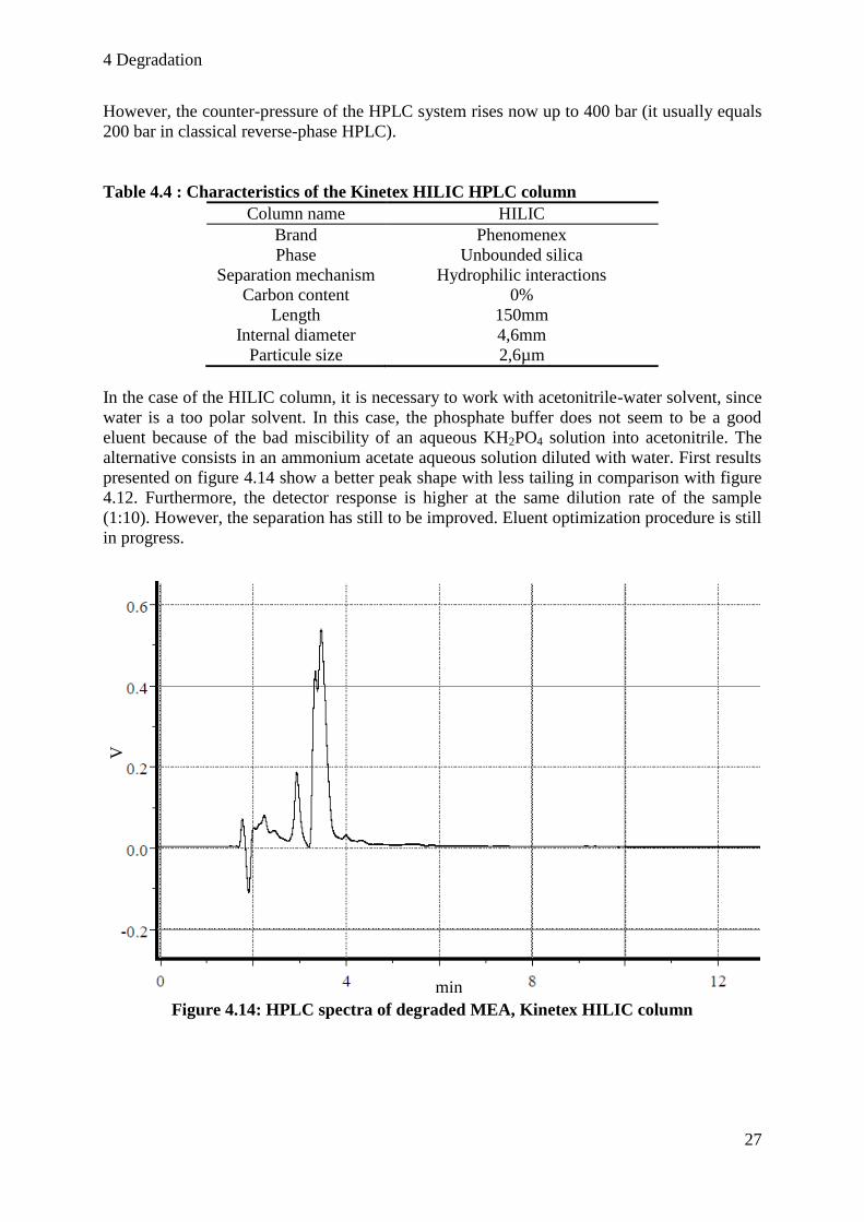
However, the counter-pressure of the HPLC system rises now up to 400 bar (it usually equals
200 bar in classical reverse-phase HPLC).
Table 4.4 : Characteristics of the Kinetex HILIC HPLC column
Column name HILIC
Brand Phenomenex
Phase Unbounded silica
Separation mechanism Hydrophilic interactions
Carbon content 0%
Length 150mm
Internal diameter 4,6mm
Particule size 2,6µm
In the case of the HILIC column, it is necessary to work with acetonitrile-water solvent, since
water is a too polar solvent. In this case, the phosphate buffer does not seem to be a good
eluent because of the bad miscibility of an aqueous KH2PO4 solution into acetonitrile. The
alternative consists in an ammonium acetate aqueous solution diluted with water. First results
presented on figure 4.14 show a better peak shape with less tailing in comparison with figure
4.12. Furthermore, the detector response is higher at the same dilution rate of the sample
(1:10). However, the separation has still to be improved. Eluent optimization procedure is still
in progress.
Figure 4.14: HPLC spectra of degraded MEA, Kinetex HILIC column
V
min

4 Degradation
28
4.3.2 Gas Chromatography (GC)
The objective of the gas chromatography analysis is to identify and quantify the amine
degradation products. The GC apparatus used for the analysis is a GC 8000 Series, made by
Fisons Instruments. It is represented on figure 4.15. The software employed is the ChromCard
Software.
Figure 4.15: Gas chromatograph
4.3.2.1 Method
The principle of the GC is the same as for the HPLC: a liquid sample is injected in a column
where the different components are eluted with different retention times, according to their
affinity with the column stationary phase. The difference is that the sample will be first
vaporized before being eluted in the chromatography column.
Before the injection, the sample is first diluted with HPLC grade water (distillated water
filtrated on 0,22µm cellulose acetate filters and degassed for 5 minutes under vacuum) in
proportion 1:50. Using a syringe, 1µl of sample is injected in the injection cell which is heated
at 280°C. The carrier gas (that replaces the eluent) is Helium. It flows continuously through
the column and its pressure is kept constant at 0,6barg. The detector is a Flame Ionization
Detector (FID) heated at 300°C.
The chromatography column is a capillary column OPTIMA-35 MS from Macherey-Nagel.
Its characteristics are presented in table 4.5.
Table 4.5 : Characteristics of the OPTIMA-35 MS GC column
Column name OPTIMA-35 MS
Brand Macherey-Nagel
Phase Cross-linked sylarene phase
4 Degradation
29
Separation mechanism Polar selectivity
Polarity Index 35 % Phenyl / 65 % Methyl-Polysiloxane
Length 30 m
Internal diameter 0,25 mm
Film thickness 0,25 µm
The column is set in an oven whose temperature is varying according to the temperature
program encoded by the operator. The whole program lasts for 60 minutes, performing the
following steps:
- T1 = 35°C during 2 minutes, then the temperature increases by 7°C/min
- T2 = 140°C, then the temperature increases by 5°C/min
- T3 = 240°C during 8 minutes, then the temperature increases by 10°C/min
- T4 = 300°C during 9 minutes.
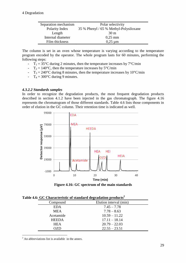
4.3.2.2 Standards samples
In order to recognize the degradation products, the most frequent degradation products
described in section 4.1.2 have been injected in the gas chromatograph. The figure 4.16
represents the chromatogram of those different standards. Table 4.6 lists those components in
order of elution in the GC column. Their retention time is indicated as well.
Figure 4.16: GC spectrum of the main standards
Table 4.6: GC Characteristic of standard degradation products2
Compound Elution interval (min)
EDA 7.45 – 7.78
MEA 7.78 – 8.63
Acetamide 10.59 – 11.22
HEEDA 17.11 – 18.14
HEA 20.79 – 22.03
OZD 22.55 – 23.51
2 An abbreviations list is available in the annex.

4 Degradation
30
HEI 25.09 – 25.93
HEIA 31.67 – 32.69
4.3.2.3 Calibration curves
The calibration curves for MEA have not been realized yet. It appears that the use of an
internal standard considerably reduces the error on the MEA quantification. 2-
Methoxyethanol (1 wt-%) is used as an internal standard. Figure 4.17 shows a spectrum in
which the internal standard is present. The method development is still under progress. The
internal standard elutes during the time laps 6,25 - 6,86 minutes, approximately one minute
before MEA, so that both peaks are well separated.
Figure 4.17: GC spectrum of MEA with internal standard
4.3.3 Fourier Transformed Infra Red analysis (FTIR)
The objective of the Fourier Transformed Infra Red spectrometer is to perform an analysis of
the gas phase emitted during the degradation reaction. Since some degradation products are
gaseous, the gaseous phase has to be analyzed to get a complete overview on degradation
reactions. One of the major oxidative degradation products of monoethanolamine is indeed
ammonia, which is emitted as a gaseous product (Chi and al, 2001; Knudsen et al, 2009).
Thanks to the FTIR analyzer, it is possible to follow the degradation rate related to ammonia.
The objective is to follow the concentration of water, CO2, ammonia and MEA in the gaseous
emissions.
This apparatus detects the infrared length waves that are absorbed by the sample. According
to the chemical bonds of the components presents in the sample, it is possible to identify the
components and to quantify them relatively to reference samples.
The FTIR is represented on figure 4.18. It is a 6700 Nicolet FTIR with a 200 ml gas cell (KBr
window, 2 meter ray pathway length). The resolution of the analyzer reaches 0,125 cm-1
. The
software related to the spectrometer is called Omnic 8.

4 Degradation
31
Figure 4.18 : FTIR analyser
4.3.3.1. Standard spectra
In order to obtain reference spectra of liquid standard like water, MEA or NH3, it has been
necessary to vaporize those elements, so that only a vapor phase reaches the FTIR analysis
cell. The vaporization occurs on a plate heated at 100°C. The liquid solution (respectively
water, NH3 in water, MEA in water) is contained in a syringe. The syringe is attached to a
syringe pump, so that the flow rate of injected solution can be precisely controlled. While the
liquid is injected through a septum on the heated plate, dried air is flowing over the heated
plate, entraining the vaporized liquid sample to the FTIR analysis cell. Figure 4.19 represents
this installation.
Figure 4.19: syringe pump and heated plate
Thanks to this installation, it was possible to analyze the IR spectrum of liquid standards.
Each compound has one or several characteristic wavelengths at which the light is absorbed
by the internal bonds. The presence and the concentration of a particular compound in the
gaseous emission can be determined by observing a characteristic wavelength interval. The
characteristic intervals for the studied compounds are presented in table 4.7.
Syringe pump
Heated plate
Air supply
Air outlet to FTIR

4 Degradation
32
Table 4.7: Characteristic absorption wavelength for FTIR analysis
Compound Wavelength interval (cm-1
)
CO2 926 – 1150
MEA 2700 – 3200
H2O 3200 – 3401
NH3 910 – 1150
However, some spectral regions are interfering. That’s why the biggest peaks associated to a
compound are rarely chosen as characteristic wavelength regions. It is the role of the FTIR
analysis to distinguish the different compounds based on calibration spectra. The different
compounds listed in table 4.7 have been identified on FTIR spectra obtained on test samples.
Figure 4.20 shows a spectrum of a CO2 – water solution.
Figure 4.20: FTIR spectrum of a CO2-H2O sample
Figures 4.21 and 4.22 are showing respectively calibration spectra for MEA and NH3.
Figure 4.21: FTIR spectrum of a MEA-H2O sample
CO2
Water
MEA

4 Degradation
33
Figure 4.22: FTIR spectrum of a NH3-H2O sample
4.3.3.2 Calibration curves
The quantification of the main gaseous compounds (H2O, MEA, NH3, CO2) using FTIR
analysis is still in progress and should be achieved by the end of 2011.
4.3.4 Ion analysis
Parallel to analytical means developed internally in the framework of this PhD thesis, some
samples have been sent to the Laboratory of Hydrogeology of the University of Liège for
analysis. Since the MEA solution is corrosive, the reactor can be damaged during the
degradation experiments. It has been observed that the stainless steel surface is modified to a
certain extent due to corrosion. In order to follow this phenomenon and to prevent the
corrosion from getting really problematic, the amount of ions present in the solution is
regularly controlled. The objective is to assess the evolution of the corrosion in the reactor.
Moreover, it may probably be possible to draw some relations between the degradation
conditions, the obtained degradation products, and the metallic ions analysis. Those relations
could give an insight on corrosion caused by the degradation products. Table 4.8 lists the
analyzed ions and the employed analytic methods for their quantification.
Table 4.8: Analysis methods of ions
Ion Method
Fe Atomic absorption
Cr Atomic absorption
Ni Atomic absorption
Si Atomic absorption
F Capillary electrophoresis
Cl Capillary electrophoresis
Iron, chromium and nickel are constituents of the T316 stainless steel. They are good
indicators to follow the corrosion. Moreover, some studies have shown that those ions can
have catalytic effect on solvent degradation (Sexton and Rochelle, 2009). Silicone has been
found in some sample but its origin remains unknown. Fluorine and Chlorine have large
effects on metal corrosion. Hence, their concentration will be systematically measured.
4.3.5 Karl-Fischer titration of water
The objective of the Karl-Fischer titration is to determine the water content of a degraded
amine sample, and to relate it to the mass loss observed during the experiment in order to
NH3

4 Degradation
34
characterize the water balance. The principle of this method is a chemical titration based on
the reaction of sulfur dioxide and iodine in the presence of water:
2 H2O + SO2 + I2 → SO42−
+ 2 I− + 4 H
+
As long as water is available in the sample, it reacts with SO2 and Iodine (this last one is
added progressively to the sample). The titration end point is detected by potentiometry as
soon as some I2 is present in excess in the sample. In the presence of an alcohol, the reactions
are slightly different, but the principle remains the same.
Each amine sample has been diluted 1:20 with Ethanol (per analysis quality). 100µl of the
diluted solution have been titrated using a 831 KF Coulometer Metrohm apparatus.
4.4 Results summary of the first tests performed
In this section, the first results obtained on the degradation test rig are presented. The
objective of the degradation test rig is to get more experimental data on accelerated amine
solvent degradation. The solvent tested is 30wt-% MEA. The influence of process parameters
like temperature, pressure, gas flow rate and composition is first studied. Different operating
modes are possible: the test rig can be operated in batch as well as in semi-batch mode, in
which case a gas continuously flows through the solution. Then, in a second test campaign,
some alternative solvent systems will be studied, including the influence of additives like
corrosion and degradation inhibitors.
First, the different experiments performed so far and their operating conditions will be
described. Since it is an experimental work, numerous practical problems have been
experienced that have slowed down the initial planning. Those experimental problems will be
briefly evocated in order to get an experimental feed-back for further tests. Then, the
analytical results obtained for each experiment will be presented and discussed. Those results
are structured as follows:
- MEA quantification by HPLC method
- GC spectra of degraded MEA samples
- Analysis of foreign ions present in solution (metals and halogens)
4.4.1 Description of the experiments
Since the beginning of the first experiment campaign in March 2011, ten experiments have
been performed to evaluate the influence of different parameters on degradation. Table 4.9
summarizes those experiments and their operating conditions.
Apart from experiments 8 and 9 which have lasted for one week, every experiment was
planned to last for 2 weeks. However, two experiments had to be stopped before the end due
to experimental problems that will be evocated further. For each experiment, a sample is
taken from the initial amine solution and from the final solution (generally after two weeks or
after one week for experiment 8 and 9). When the experiment had to be stopped before term, a
sample was taken just before stopping the experiment. Those samples were conserved in a
fridge until the analysis in order to stop the degradation reactions.
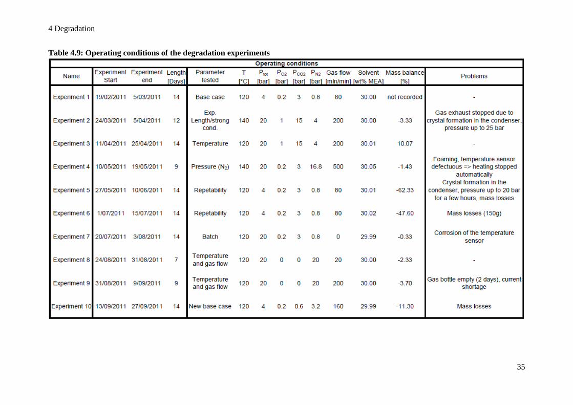
4 Degradation
35
Table 4.9: Operating conditions of the degradation experiments

4 Degradation
36
4.4.2 Experimental feed-back
Many experimental problems have been experienced during this first test campaign. Next to
numerous minor problems like gas leakages, solution foaming by high gas flow, pressure
oscillations… some major problems occur regularly. Those problems are briefly described in
this section in order to draw a feed-back that could be helpful for further experimental works.
The main problems experienced are listed below:
- Corrosion: the amine solvents and the degradation products are corrosive to stainless
steel, included T316. The first traces of corrosion have been detected very early in the
reactor vessel. A long passivation procedure has then been performed with
successively distilled water and nitric acid in order to protect the metal surface from
further attacks. It appears now that although the passivation was necessary, a rough
passivation would have been enough and would have saved a lot of time.
The conclusion was that corrosion cannot be prevented. It continuously takes place in
the degradation reactor, but it is regularly controlled by conductivity measurement and
ion analysis to be sure it doesn’t dramatically increase. Since metal and halogen ions
are implied in the corrosion phenomenon, their concentration in the solution is
measured after each experiment so that the corrosion can be followed up.
- Crystal formation: The gas exiting the degradation reactor flows up into a condenser
where it is cooled down, as described in section 4.2.3. The liquid condensate normally
refluxes to the reactor. However, the diameter of the reflux pipe is relatively small and
in some place, the liquid is stagnating, leading to crystallization of the liquid. Those
crystals accumulate and finally form a plug, so that the gas cannot exit the reactor
anymore. This leads to an undesired pressure increase. The first time that this problem
occurred, the experiment had to be stopped before its term. Once the problem has been
identified, it was possible to clean the condenser without stopping the experiment.
- Mass balance regulation: the regulation of the mass balance is a problem that has
been reported in the literature by all research groups performing semi-batch
experiments with continuous gas flow. Since gas flows through an aqueous liquid, it is
saturated with water when exiting the reactor. In order to minimize the water loss, it is
condensed at the reactor exit and saturated with water before flowing into the reactor.
Condensation and saturation take place at the same temperature. However, the mass
balance of the solution, i.e. the liquid weight difference between the experiment start
and the experiment end often fluctuates (see table 4.9).
This problem has not been solved yet. However, in order to quantify the impact of this
fluctuation on the amine concentration, it has been decided to measure the water
concentration of initial and final samples by Karl-Fischer titration.
- Temperature regulation: One experiment (experiment 4) had to be stopped before
term because of a defective connection on the temperature sensor controlling the
reactor temperature. This triggered the test rig emergency shut-down. The sensor was
replaced by another in-house sensor, which appeared to be much more sensitive to
corrosion. Finally, a new sensor was purchased. It was also necessary to repair the
original heating mantle of the reactor which induced an electrical shortcut.

4 Degradation
37
- Agitation: the agitation shaft furnished with the reactor appeared to be not perfectly
straight. This implied some damages on the PTFE bushing connecting the agitator to a
guide fixed to the cooling coil (see figure 4.23). As a result, Fluorine was detected
during the halogen ions analysis in the amine solution. Fluorine may have been
released from the PTFE bushing due to mechanical rubbing caused by the non
centered rotation of the agitator.
Figure 4.23: Guide with PTFE bushing for the agitator support
4.4.3 HPLC Quantification of MEA degradation
The objective of the HPLC analysis is to quantify the MEA concentration in the degraded
solution at the end of the experiment. For each experiment, the final sample has been diluted
10 times with distillated water before injection.
Figure 4.24 represents the MEA concentration for each experiment. The results can be seen in
table 4.10 as well. The initial concentration was always 30 wt-% MEA (see also table 4.9).
The mean error value has been calculated and equals 2%.

4 Degradation
38
0
5
10
15
20
25
30
35
40
1 2 3 4 5 6 7 8 9 10
Experiment number
MEA
co
nce
ntr
atio
n (
wt-
%)
Figure 4.24: MEA concentrations measured during the degradation experiments
Table 4.10: MEA concentration at the experiments’ end
Experiment MEA concentration (wt-%) MEA concentration change (%)
1 27.79 -7.4
2 12.57 -58.1
3 17.93 -40.2
4 25.44 -15.2
5 25.44 -15.2
6 35.07 +16.9
7 19.02 -36.6
8 30.16 +0.5
9 30,79 +2.6
10 24.80 -17.3
Those results must be considered in parallel with the mass balance data. It is the only way to
explain that the MEA concentration sometimes increases: in fact, some water is evaporated
and exits the reactor, so that the relative amine concentration increases, even if the total amine

4 Degradation
39
amount remains unchanged. This is the case by Experiments 8 and 9: no degradation could be
observed, which confirms that in the absence of O2 and CO2, degradation can be neglected,
even at 120°C. The absence of degradation was confirmed by the GC spectra (see section
4.4.4) and the sample color, identical to non-degraded MEA. In the case of Experiment 6
however, the sample color was like degraded MEA, very dark. The high MEA concentration
is clearly due in this case to the water losses. In order to solve this incertitude, the samples
will be analyzed for water content using a Karl-Fisher titration. The samples have been sent
for analysis and results should be available within a few weeks.
When comparing the results with the base case results (Experiment 1), some conclusions can
be drawn. First, the degradation observed by the Experiment 2 is as expected the highest since
the operating conditions were effectively the strongest in that case. Then, it is possible to see
that the temperature has an important impact on the degradation, since the only difference
between experiments 2 and 3 is that the temperature has been decreased to 120°C instead of
140°C. We can see that operating the degradation test rig in batch mode leads to high
degradation rate as well.
Finally, working at high N2 pressure low O2 and CO2 content does not lead to strong
degradation as it can be observed from Experiment 4. Experiment 1 and 4 show
approximately the same final MEA concentration. The difference could be explained by the
temperature difference between both experiments.
It is important to observe that repeatability could not be achieved so far, mainly due to mass
balance problems in the reactor.
4.4.4 GC spectra of degraded MEA
The final samples of Experiments 1 to 10 have been analyzed using gas chromatography. The
first objective is to draw qualitative results about the degradation products contained in the
samples. In a second analysis phase, those degradation products shall be quantified.
Since the degradation extent is different depending on the experiments, some samples have
been diluted 10 times and other 50 times with distillated water before the injection. The
chromatograms are presented in this section.
On figure 4.25, we can distinguish the MEA peak, as well as seven other degradation
products. Some products can already be identified as shown in table 4.11.

4 Degradation
40
Figure 4.25: GC spectrum of Experiment 1, final sample, diluted 1:10
Table 4.11: Main degradation products in Experiment 1
Compound Elution interval (min) Maximum (µV)
MEA 8.17 – 10.72 156 304
OZD 22.53 – 22.74 647
HEI 24.98 – 25.59 538
HEIA 31.37 – 31.89 1259
Product 1 32.44 – 32.73 575
Product 2 34.16 – 35.29 9525
Product 3 35.53 – 36.01 457
Product 4 38.63 – 39.83 904
The same analysis can be performed for the other experiments: see Figures 4.26 to 4.34 and
Tables 4.12 to 4.20
Figure 4.26: GC spectrum of Experiment 2, final sample, diluted 1:10
Table 4.12: Main degradation products in Experiment 2
Compound Elution interval (min) Maximum (µV)
MEA 7.56 – 8.79 87424
Acetamide 10.48 –10.9 1517
Product 5 19.84 – 20.06 2458
Product 6 20.46 – 20.76 3444
OZD 22.49 – 22.60 2329
HEI 24.92 – 25.12 5002
Product 7 25.62 – 25.68 1491
Product 8 31.42 – 31.6 7306
HEIA 31.6 – 32.00 7306
Product 1 32.52 – 32.63 2470
Product 2 34.26 – 35.19 24562
Product 3 35.62 – 36.79 685
Product 4 38.71 – 39.04 4826

4 Degradation
41
Figure 4.27: GC spectrum of Experiment 3, final sample, diluted 1:10
Table 4.13: Main degradation products in Experiment 3
Compound Elution interval (min) Maximum (µV)
MEA 7.42 – 8.97 93184
Acetamide 10.22 – 10.48 569
Product 5 19.80 –20.16 863
Product 6 20.40 – 20.53 674
Product 9 21.40 – 21.49 772
OZD 22.38 – 22.56 2222
HEI 24.81 – 25.64 7629
Product 10 25.87 – 26.03 1017
Product 11 26.18 – 26.43 632
Product 12 27.93 – 27.98 601
Product 2 34.18 – 34.88 10420
Product 3 35.47 – 35.60 745
Product 4 38.55 – 39.01 5631

4 Degradation
42
Figure 4.28: GC spectrum of Experiment 4, final sample, diluted 1:10
Table 4.14: Main degradation products in Experiment 4
Compound Elution interval (min) Maximum (µV)
MEA 7.38 – 9.75 96072
Product 13 11.55 – 12.22 1155312
OZD 22.40 – 22.57 103
HEI 24.84 – 25.21 1822
HEIA 31.34 – 32.18 4891
Product 1 32.18 – 32.63 638
Product 2 34.13 – 35.70 11889
Product 4 38.70 – 39.47 215
Figure 4.29: GC spectrum of Experiment 5, final sample, diluted 1:10
Table 4.15: Main degradation products in Experiment 5
Compound Elution interval (min) Maximum (µV)
MEA 7.24 – 9.90 155560
Product 14 9.90 – 10.31 2104
Acetamide 10.31 – 12.18 1627
HEEDA 16.94 – 17.21 281
Product 5 19.90 – 20.59 9875
Product 6 20.60 – 21.04 6306
Product 9 21.38 – 21.60 186
Product 15 22.18 – 22.40 556
OZD 22.49 – 22.69 1131
Product 16 23.72 – 23.82 329
HEI 24.96 – 25.51 5520
Product 7 25.66 – 25.92 1844
Product 12 28.07 – 28.22 933
Product 17 30.45 – 30.60 1219
Product 18 31.03 – 31.26 1594

4 Degradation
43
Product 8 31.45 – 31.72 10905
HEIA 31.73 – 32.31 8017
Product 1 32.53 – 33.20 7557
Product 19 33.66 – 34.02 1850
Product 2 34.24 – 35.80 71704
Product 3 35.81 – 36.82 5689
Product 20 37.06 – 37.89 2079
Product 4 38.88 – 39.09 1536
Product 21 40,20 – 40,47 114
Product 22 40.87 – 41.34 2386
Figure 4.30: GC spectrum of Experiment 6, final sample, diluted 1:10
Table 4.16: Main degradation products in Experiment 6
Compound Elution interval (min) Maximum (µV)
MEA 7.82 – 10.16 171352
Product 14 10.17 – 10.39 2429
Acetamide 10.60 – 10.99 1767
HEEDA 16.96 – 17.11 1066
Product 23 17.85 – 18.74 2355
Product 5 19.94 – 20.73 10573
Product 6 20.74 – 21.11 8396
Product 15 22.16 – 22.40 2536
OZD 22.40 – 22.80 3041
Product 16 23.63 – 23.71 1116
HEI 24.83 – 25.56 11682
Product 7 25.57 – 25.90 2964
Product 24 26.90 – 27.41 4495
Product 12 28,00 – 28.11 1391
Product 18 31.03 – 31.13 1745
Product 8 31.37 – 31.71 16451
HEIA 31.72 – 32.52 17619
Product 1 32.53 – 32.90 5416
Product 19 33.55 – 34.17 8599

4 Degradation
44
Product 2 34.25 – 35.29 30928
Product 3 35.69 – 36.18 4440
Product 20 37.10 – 37.40 2174
Product 4 38.75 – 38.95 3156
Product 21 40.00 – 40.34 1445
Product 22 40.72 – 40.99 1472
Product 25 44.13 – 44.43 1467
Figure 4.31: GC spectrum of Experiment 7, final sample, diluted 1:10
Table 4.17: Main degradation products in Experiment 7
Compound Elution interval (min) Maximum (µV)
MEA 7.27 – 9.53 121976
Acetamide ? 11.26 – 11.40 726
HEEDA 17.13 – 18.69 1956
Product 5 20.12 – 20.45 981
OZD 22.53 – 22.77 760
HEI 24.65 – 25.03 801
Product 18 31.14 – 31.42 1989
HEIA 31.57 – 32.25 32416
Product 2 34.54 – 34.85 2138
Product 20 37.04 – 37.64 22373
Product 26 37.65 – 38.97 12294
Product 27 41.52 – 41.84 1249
Product 28 42.24 – 42.79 8010
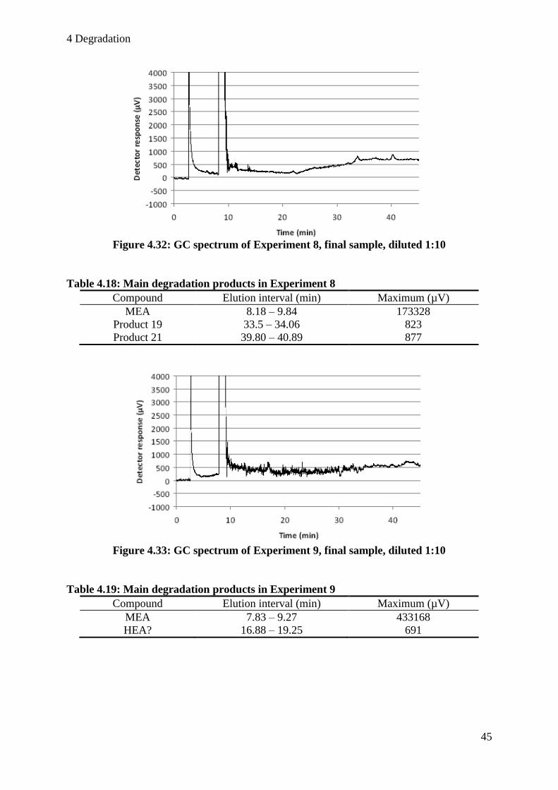
4 Degradation
45
Figure 4.32: GC spectrum of Experiment 8, final sample, diluted 1:10
Table 4.18: Main degradation products in Experiment 8
Compound Elution interval (min) Maximum (µV)
MEA 8.18 – 9.84 173328
Product 19 33.5 – 34.06 823
Product 21 39.80 – 40.89 877
Figure 4.33: GC spectrum of Experiment 9, final sample, diluted 1:10
Table 4.19: Main degradation products in Experiment 9
Compound Elution interval (min) Maximum (µV)
MEA 7.83 – 9.27 433168
HEA? 16.88 – 19.25 691

4 Degradation
46
Figure 4.34 : GC spectrum of Experiment 10, final sample, diluted 1:10
Table 4.20: Main degradation products in Experiment 10
Compound Elution interval (min) Maximum (µV)
MEA 7.57 – 9.51 150816
Product 5 20.02 – 20.30 678
Product 6 20.53 – 20.80 888
Product 29 21.09 – 21.37 1024
Product 9 21.38 – 22.24 926
OZD 22.46 – 22.78 1396
HEI 24.90 – 25.88 1668
HEIA 31.44 – 31.76 914
Product 1 32.49 – 32.77 803
Product 2 34.26 – 35.51 9946
Product 3 35.52 – 36.22 4830
Product 20 37.13 – 37.79 1128
Product 4 38.73 – 39.33 2719
Table 4.21 summarizes the previous results. Most of the unknown products that appear only
once in the previous spectra may be due to contaminations, or detection errors. However,
many of those products appear regularly, as it can be observed in Table 4.21. It could be
interesting to identify those products for a better understanding of the degradation
phenomena.
Table 4.21: Degradation products in each experiment
Experiment
Product
1 2 3 4 5 6 7 8 9 10
MEA x x x x x x x x x x
Acetamide x x x x x
HEEDA x x x
HEA x
OZD x x x x x x x x
HEI x x x x x x x x

4 Degradation
47
HEIA x x x x x x
Product 1 x x x x x x
Product 2 x x x x x x x x
Product 3 x x x x x
Product 4 x x x x x x
Product 5 x x x x x x
Product 6 x x x x x
Product 7 x x x
Product 8 x x x x
Product 9 x x x
Product 10 x
Product 11 x
Product 12 x x x
Product 13 x
Product 14 x x
Product 15 x x
Product 16 x x
Product 17 x
Product 18 x x x
Product 19 x x x
Product 20 x x x x
Product 21 x x x
Product 22 x x
Product 23 x
Product 24 x
Product 25 x
Product 26 x
Product 27 x
Product 28 x
Product 29 x
4.4.5 Ion analysis results
In order to follow the corrosion phenomena that take place inside the degradation reactor, it
has been decided to measure the quantity of some particular metal and halogen ions that play
a role in corrosion. After each degradation experiment, samples are sent to the Laboratory for
Hydrogeology of the University of Liège where the samples are analyzed. Table 4.22 presents
the evolution of ions in solution.
Table 4.22: Evolution of ion concentrations in solution, in ppm
Fe
Cr
Ni Si Cl F
MEA 30% 0.44 < 0.10 < 0.10 -a
< 2.00 38.944
Experiment 1 7.57 1.55 4.24 -a
< 2.00 416.08
Experiment 2 22.40 8.60 9.75 13.01 513.16 1826.18
Experiment 3 6.80 3.10 2.66 10.66 522.32 869.35

4 Degradation
48
Experiment 4 1.90 1.30 1.01 15.57 291.36 307.13
Experiment 6b
14,70 2.75 159 2754.21 < 5.00 594.62
Experiment 7
66.10 7.50 571 147.78 < 5.00 321.14
Experiment 8 0.19 2.27 0.69 94.80 < 5.00 251.55
Experiment 9 0.14 2.39 0.51 95.55 < 5.00 276.30
Experiment 10 3.46 6.41 0.87 557.55 29.34 532.38 a
Silicon has not been measured for the two first samples b
Final sample from Experiment 5 still has to be analyzed
Iron, Chromium, and Nickel concentrations are most of the time really well correlated. These
three metals are present in T316 stainless steel. When their concentration is high, it means
that the reactor has been damaged by the amine solution and that a lot of those ions dissolved
in the liquid phase. Based on this assumption, it is possible to conclude that some degradation
products presents in Experiments 2, 6 and 7 are very corrosive.
What concerns the concentration of Chlorine and Fluorine, they are not related to the metal
ions concentrations (see Experiment 4 for instance). However, it is known that Chlorine and
Fluorine are very corrosive elements. We can conclude from this that Chlorine and Fluorine
are not influencing the corrosion of the degradation vessel. However, their presence and the
way they vary remain unexplainable, especially for Chlorine since the presence of Fluorine
could be explained by the problems related to the agitator described in section 4.4.2. The
presence of Silicon remains unexplainable as well. One possible hypothesis is that some
Silicon may come from lubricant used in the magnetic agitation system of the reactor.
However, it is possible to deduce from the results presented here that Silicon has no influence
on corrosion either.
The follow-up of corrosion will continue during the next experiments. Moreover, a detailed
inspection of the reactor vessel by corrosion experts from Laborelec is planned to be sure that
corrosion remains under control.
4.4.6 Karl-Fischer titration results
The results obtained by the Karl-Fischer titration are presented in table 4.23. The objective is
to correlate them with the mass losses results recorded during the degradation experiments.
Consequently, the relative amount of evaporated water during the experiment can be
determined and the mass balance can be checked. Figure
Table 4.23: Results of the KF analysis and comparison with mass balance results
Experiment Water balance
Mass balance
Experiment 1 -9% Not recorded
Experiment 2 2% -3%
Experiment 3 -3% +10%
Experiment 4 -3% -1%
Experiment 5 -36% -62%
Experiment 6 -49% -48%
Experiment 7
0% 0%
Experiment 8
-1% -2%
Experiment 9 -4% -4%
Experiment 10 -8% -11%

4 Degradation
49
-70
-60
-50
-40
-30
-20
-10
0
10
20
1 2 3 4 5 6 7 8 9 10
Experiment number
Mas
s an
d w
ater
ba
lan
ces
(%)
Water balance Mass balance
Figure 4.35: Results of the KF analysis and comparison with mass balance results
We can see that both results are quite well correlated, which means that mass losses and water
losses vary during degradation experiments in the same proportions.

5 Conclusion and perspectives
50
5 Conclusion and perspectives
The present report describes the work that has been performed the last two years in the
framework of a PhD thesis at the University of Liège. This work results from a collaboration
between the company Laborelec and the University of Liège. The application fields of this
thesis are divided into two main parts.
First, the simulation of the post-combustion CO2 capture process in a coal-fired power
installation with monoethanolamine is studied using two different models. The first model
makes some equilibrium assumptions regarding the mass transfer columns and neglects
geometry and kinetics parameters. The second model takes those parameters into account. For
each model, the simulation has been performed in two steps. The first step consisted in the
identification and the sensitivity study of process parameters having a large influence on the
capture energetic efficiency. The second step consisted in the implementation of process
modification with the same goal of reducing the energy requirement of the CO2 capture.
Those studies have shown that it was possible to save about 20% of the solvent regeneration
energy while performing those modifications. However, the model still has to be validated to
be completely reliable. Experimental data for validation purpose shall be obtained from the
mobile pilot capture installation actually located in Gelderland and for which Laborelec takes
part to the development.
The second objective is to perform an experimental study of solvent degradation in the case of
CCS solvents. Since the cost related to solvent replacement reaches approximately 22% of the
OPEX (Abu Zahra, 2009), it is essential to consider solvent degradation prior to any scale-up
operation. In this optic, a test rig has been built at the University of Liège to assess the
degradation of solvents under accelerated degradation conditions. This equipment allows for
batch and semi-batch studies, in which a gas mix is continuously bubbling through the solvent
solution. High pressure and high temperature conditions may be imposed in order to
accelerate the degradation phenomena. The results of the first test campaign are presented in
this report. Different analytical means have been developed to assess precisely the solvent
degradation in the liquid phase, as well as in the gas phase. The development of those
methods is still under progress, but good results have been recorded, especially using Gas
Chromatography and High Performance Liquid Chromatography. Many experimental
problems have been met and solved, so that the second test campaign may allow a complete
characterization of monoethanolamine degradation. Perspectives regarding degradation
studies also include the test of additives such as degradation inhibitors.
Finally, the main objective of the PhD thesis is to develop a validated simulation model
including degradation data. Based on this model, it will be possible to perform a multi-
objective optimization of the CO2 capture process, considering the influence of key process
parameters on regeneration energy requirement as well as on degradation extent. Based on a
cost approach, this multi-objective optimization should lead to a proposition for optimal
operating conditions regarding energy efficiency as well as degradation and environmental
performance.

6 Bibliography
51
6 Bibliography Abu Zahra M., 2009, Carbon dioxide capture from flue gas, PhD Thesis at Delft University,
Netherlands
Aspen Tech, 2011, Apr System Help, Electrolyte NRTL, Development of the Model
Bedell S., 2009, Oxidative degradation mechanisms for amine in flue gas capture, Energy
Procedia 1 (2009) 771–778
Bello A. and Idem R., 2005, Pathways for the Formation of Products of the Oxidative
Degradation of CO2-Loaded Concentrated Aqueous Monoethanolamine Solutions during CO2
Absorption from Flue Gases, Ind. Eng. Chem. Res. 2005, 44, 945-969
Bello A. and Idem R., 2006, Comprehensive Study of the Kinetics of the Oxidative
Degradation of CO2 Loaded and Concentrated Aqueous Monoethanolamine (MEA) with and
without Sodium Metavanadate during CO2 Absorption from Flue Gases, Ind. Eng. Chem. Res.
2006, 45, 2569-2579
Bacot S., Picq D., Carrette P-L., Kittel J., 2007, Nouvelles amines permettant le captage du
CO2 : dégradation et corrosivité, projet CapCO2, Présentation réalisée à Pau,12 et 13
décembre 2007
Captech, 2008, Advanced Solvent Development at Shell, 2nd CAPTECH Day, Arnhem, 06.
March 2008
Chi S., Rochelle, G., 2001, Master Thesis, Oxidative Degradation of Monoethanolamine,
University of Texas at Austin, USA
Davis J., 2009, Thermal Degradation of Aqueous Amines Used for Carbon Dioxide Capture,
PhD Thesis, University of Texas at Austin, USA
Davis J., Rochelle, G., 2009, Thermal degradation of monoethanolamine at stripper
conditions, Energy Procedia 1, 2009 327-333
Dubois L., Thomas D., 2009, CO2 Absorption into Aqueous Solutions of Monoethanolamine,
Methyldiethanolamine, Piperazine and their Blends, Chem. Eng. Technol. 2009, 32, No. 5, 1–
10
Goff and Rochelle, 2004, Monoethanolamine Degradation: O2 Mass Transfer Effects under
CO2 Capture Conditions, Ind. Eng. Chem. Res. 2004, 43, 6400-6408
Goff, 2005, Oxidative degradation of aqueous MEA in CO2-capture processes: Iron and
copper catalysis, Inhibition and O2 mass transfer, PhD Thesis, University of Texas at Austin,
USA
Goff and Rochelle, 2006, Oxidation Inhibitors for Copper and Iron Catalyzed Degradation of
Monoethanolamine in CO2 Capture Processes, Ind. Eng. Chem. Res. 2006, 45, 2513-2521
IPCC, 2005, IPCC special report on carbon dioxide capture and storage, Cambridge
university press

6 Bibliography
52
Kaminski, M.; Jastrzebski, D.; Przyjazny, A.; Kartanowicz, R., 2002, Determination of the
Amount of Wash Amines and Ammonium Ion in Desulfurization Products of Process Gases
and Results of Related Studies, J. Chromatogr. A 2002, 947, 217.
Knudsen J., Jensen J., Vilhelmsen P., Biede O., 2007, First year operation experience with a
1 t/h CO2 absorption pilot plant at Esbjerg coal-fired power plant Proceedings of European
Congress of Chemical Engineering (ECCE-6) Copenhagen, 16-20 September 2007
Knudsen J., Vilhelmsen P., Jensen J., Biede O., 2009, Experience with CO2 capture from
coal flue gas in pilot scale, Energy proceedia 1, 2009, 783-790.
Lawal A. and Idem R., 2005, Effects of Operating Variables on the Product Distribution and
Reaction Pathways in the Oxidative Degradation of CO2- Loaded Aqueous MEA-MDEA
Blends during CO2 Absorption from Flue Gas Streams, Ind. Eng. Chem. Res. 2005, 44, 986-1003
Lawal A., Bello A. and Idem R., 2005, The Role of Methyl Diethanolamine (MDEA) in
Preventing the Oxidative Degradation of CO2 Loaded and Concentrated Aqueous
Monoethanolamine (MEA)-MDEA Blends during CO2 Absorption from Flue Gases, Ind.
Eng. Chem. Res. 2005, 44, 1874-1896
Lawal A. and Idem R., 2006, Kinetics of the Oxidative Degradation of CO2 Loaded and
Concentrated Aqueous MEA-MDEA Blends during CO2 Absorption from Flue Gas Streams,
Ind. Eng. Chem. Res. 2006, 45, 2601-2607
Lawal A., Wang M., Stephenson P., Yeung H., 2008, Dynamic modelling of CO2 absorption
for post combustion capture in coal-fired power plants, Fuel, doi:10.1016/j.fuel.2008.11.009
Léonard G., 2009, Modeling of a pilot plant for the CO2-reactive absorption in amine solvent
for power plant flue gases, Master Thesis at University of Liège, Belgium
Lepaumier H., 2008, Etude des mécanismes de dégradation des amines utilisées pour le
captage du CO2 dans les fumées, PhD thesis at the University of Savoie, France
Lepaumier H., Picq D., Carrette P., 2009, Degradation Study of new solvents for CO2
capture in post combustion, Energy Procedia 1, 2009, 893-900
Lepaumier H., da Silva E., Einbu A., Grimstvedt A., Knudsen J., Zahlsen K., Svendsen H.,
2010, Comparison of MEA degradation in pilot-scale with lab-scale experiments, Energy
Procedia 4, 2011, 1652–1659
Notz R., Asprion N., Clausen I. and Hasse H., 2007, Selection and pilot plant tests of new
absorbents for post-combustion carbon dioxide capture, doi: 10.1205/cherd06085
Notz R., 2009, CO2-Abtrennung aus Kraftwerksabgasen mittels Reaktivabsorption, PhD
Thesis at the University of Stuttgart, Germany
Sexton A., 2008, Amine oxidation in CO2 capture processes, PhD Thesis at the University of
Texas at Austin, Texas, USA.

6 Bibliography
53
Sexton and Rochelle, 2009, Catalysts and Inhibitors for MEA Oxidation, Energy Procedia 1,
2009, 1179–1185
Supap T., Idem R., Veawab A., Aroonwilas A., Tontiwachwuthikul P., Chakma A., Kybett
B., 2001, Kinetics of the Oxidative Degradation of Aqueous Monoethanolamine in a Flue Gas
Treating Unit, Ind. Eng. Chem. Res. 2001, 40, 3445-3450
Supap T., Idem R., Tontiwachwuthikul P. and Saiwan C., 2006, Analysis of
Monoethanolamine and its Oxidative Degradation Products during CO2 Absorption from Flue
Gases: A Comparative Study of GC-MS, HPLC-RID, and CE-DAD Analytical Techniques
and Possible Optimum Combinations, Ind. Eng. Chem. Res. 2006, 45, 2437-2451
Supap T., Idem R., Tontiwachwuthikul P. and Saiwan C., 2009, Kinetics of sulfur dioxide-
and oxygen-induced degradation of aqueous Monoethanolamine solution during CO2
absorption from power plant flue gas streams, International Journal of greenhouse gas control
3, 2009, 133–142
Uyanga I. and Idem R., 2007, Studies of SO2- and O2-Induced Degradation of Aqueous MEA
during CO2 Capture from Power Plant Flue Gas Streams, Ind. Eng. Chem. Res. 2007, 46,
2558-2566
Zhang Y., Chen H., Chen C.-C., Plaza J., Dugas R., Rochelle G., 2009, Rate-based process
modeling of CO2 capture with aqueous monoethanolamine solution, Ind. Eng. Chem. Res.,
48, 9233–9246
7 Abbreviation List
54
7 Abbreviation List
EDA Ethylenediamine
FID Flame Ionization Detector
FTIR Fourier Transform Infra Red analysis
GC Gas Chromatography
HEA N-acetylethanolamine
HEEDA 2-(2-Aminoethylamino)ethanol
HEI 1-(2-Hydroxyethylimidazole)
HEIA 1-(2-Hydroxyethyl)-2-imidazolidinone
HPLC High Performance Liquid Chromatography
IC Intercooling
KF Karl Fischer
LVC Lean Vapor Compression
MEA Monoethanolamine
OZD Oxazolidone
PTFE Polytetrafluoroethylene (Teflon®
)
RID Refractive Index Detector

8 Appendices
55
8 Appendices
8.1 Risk analysis for the Degradation Test Rig.
This section describes in French the risk analysis that has been performed for the degradation
test rig.
8.1.1 Les locaux et zones de travail
Le banc de dégradation des solvants CCS construit dans le cadre de la thèse de doctorat de G.
Léonard en collaboration avec l’entreprise Laborelec se situe à la Halle de Chimie Appliquée
(figure 1) à l’adresse suivante :
Halle de Chimie Appliquée,
B17, P35, Grande traverse
4000 Liège Sart-Tilman.
Tel. : 04/366 44 62
L’accès à la Halle se fait par une porte sur laquelle un affichage indique clairement que
l’accès est réservé aux seules personnes autorisées ou accompagnées. En dehors des heures
d’ouvertures, cette porte est fermée à clé et une alarme est activée à l’intérieur du bâtiment.
Fig. 1 : B17, Halle de chimie appliquée Fig. 2 : Porte d’accès à la Halle
Les activités de la halle concernent le génie chimique et génie des procédés. Les principales
activités sont les suivantes : études hydrodynamiques de cuves agitées et de colonnes à
empilage, tomographie rayons X, isothermes d’adsorption de polluants, séchage de boues
d’épuration, …
Le réacteur de dégradation se situe à l’intérieur d’un local ventilé fermé, lui-même à
l’intérieur d’une pièce ouverte sur la Halle (voir plan ci-dessous, figure 3). Il y a 2 entrées /
sorties à la Halle, et les flèches rouges sur la figure 3 symbolisent les voies d’évacuation du
bâtiment.

8 Appendices
56
Main entrance andemergency exit
Degradation reactorin a ventilated room
Building of applied chemistry
Labs
FTIR analyser
Control panel
TechnicalworkshopSecondary entrance
and emergency exit
Gas cylinders
Meeting room
Storage roomfor chemicals
Fig. 3 : Plan de la halle de chimie appliquée
8.1.2 L’organisation technique entre postes de travail
L’installation de dégradation est composée de quatre parties principales (figures 4 à 7) :
- un local ventilé où se trouvent le réacteur et ses auxiliaires (figure 4)
- dans un deuxième local ventilé voisin de celui où se trouve le réacteur : l’analyseur
FTIR (figure 5)
- à côté du local ventilé où se trouve le réacteur : le poste de contrôle, l’analyseur HPLC
et les lignes d’arrivée du gaz (figure 6)
- à l’entrée de la pièce ouverte, côté Halle : les bouteilles de gaz et leur centrale de
détente (figure 7).
Fig. 4 : local ventilé Fig. 5 : Analyseur FTIR

8 Appendices
57
Fig. 6 : Poste de contrôle Fig. 7 : Rack à bouteilles
Le local ventilé où se situe le réacteur de dégradation peut accueillir une personne qui
manipule l’installation. Ce local doit être fermé durant les manipulations entre les expériences
ainsi que lors des expériences.
La pièce dans laquelle se situe ce local ventilé est partagée entre deux utilisateurs réguliers.
Le premier utilisateur régulier travaille sur l’installation située dans le même local ventilé que
l’analyseur FTIR. Le deuxième utilisateur régulier est l’opérateur du banc de dégradation.
Occasionnellement, d’autres utilisateurs pénètrent dans cette pièce pour avoir accès aux
machines qui s’y trouvent (étuve, centrifugeuse).
Cette pièce a une seule porte d’accès, tout comme le local ventilé. Les voies de circulation
dans la pièce sont clairement délimitées. L’accès aux zones de travail se fait sans problème.
L’encombrement devra être limité au strict nécessaire, et des rangements réguliers (une fois
tous les mois au minimum) seront prévus pour éviter l’accumulation de matériel dans les
locaux et zones de travail.
8.1.3 Prévention des accidents de travail
Fig. 8 : Equipements de protection individuelle
La boite de premiers soins se trouve près des toilettes, à côté de la salle de réunion.
La procédure à appliquer en cas d’accident est celle applicable de manière générale dans les
laboratoires de l’ULg. Cette procédure est à suivre en cas d’urgence lors d’un fonctionnement
défectueux de l’installation de dégradation et dans le cas où les alarmes automatiques ne se
Les équipements de protection individuelle
nécessaires sont disponibles à la halle : tabliers
de laboratoires, lunettes de protection, gants
adaptés à la manipulation de solutions aminées.
Ils se trouvent dans une armoire située à côté
de la porte d’entrée de la pièce ouverte sur la
Halle (figure 8). Dans cette armoire se trouve
également un flacon de produit nettoyant pour
rincer les yeux en cas de contact avec un
produit non désirable. La durée de validité de
ce produit est contrôlée régulièrement.

8 Appendices
58
seraient pas déclenchées. Cette procédure se trouve en première page de la farde
accompagnant l’installation et qui se trouve près du panneau de contrôle.
Le fonctionnement défectueux du banc d’essai est constaté lorsque :
- une fuite importante de gaz ou de liquide audible ou observable par le hublot fixé sur
la porte du local ventilé ou sur la ligne de gaz en dehors du local ventilé permet de
conclure que l’installation n’est pas dans un mode de fonctionnement habituel ou
prévu par l’opérateur, entraînant l’apparition d’un danger potentiel pour le personnel
ou le matériel à proximité.
- Une valeur anormale d’un capteur de température ou de pression est constatée,
entraînant l’apparition d’un danger potentiel pour le personnel ou le matériel à
proximité.
- Un bruit anormal lié à l’installation permet de conclure que l’installation n’est pas
dans un mode de fonctionnement habituel ou prévu par l’opérateur, entraînant
l’apparition d’un danger potentiel pour le personnel ou le matériel à proximité.
- tout autre élément significatif amenant à cette même conclusion.
La procédure à suivre en cas d’urgence est dès lors la suivante :
1. Arrêt immédiat de l’installation au moyen du bouton d’arrêt d’urgence situé sur la
cloison extérieure du local ventilé
2. Arrêt du chauffage du réacteur sur le poste de contrôle situé juste à coté du local
ventilé.
3. Fermeture manuelle des vannes de sécurité commandant l’arrivée de gaz au niveau des
détendeurs
4. Fermeture manuelle des vannes sur les bouteilles de gaz
5. Si quelqu’un est présent dans le local ventilé où se trouve le réacteur, évacuer ce local
en refermant bien la porte
6. Si la ventilation du local ventilé n’est pas activée, mise en route de la ventilation au
moyen de l’interrupteur situé sur la cloison extérieure de ce local
7. En cas de danger persistant, évacuer le bâtiment en s’assurant que tout le personnel
présent à l’intérieur de la halle est évacué
8. Contacter le service d’urgence au 100 (Service médical d’urgence et pompiers) ou au
112 (numéro d’appel européen en cas d’accident ou d’agression)
9. Contacter le Central d’alarme de l’ULg au numéro 04/366 44 44 (44 44 si appel
interne)
10. Contacter le personnel responsable de l’installation au numéro suivant : 04/366 95 92
ou 0487/47 11 35 (GSM Grégoire Léonard).
8.1.4 Les risques électriques
L’installation électrique a été effectuée par le personnel qualifié en suivant les normes en
vigueur. Différentes protections ont été prévues pour limiter les conséquences de tout
dysfonctionnement électrique. Entre autres :
- un différentiel 30mA protège l’installation et ses utilisateurs en coupant l’alimentation
lorsque des courants de fuite sont détectés,
- un fusible coupe le courant en cas de court-circuit ou de surintensité du courant à
l’installation
- une prise de terre est établie selon les normes en vigueur et toute l’installation y est
électriquement reliée.

8 Appendices
59
L’appareillage électrique se situe dans un coffret facile d’accès à l’intérieur du local ventilé
(figure 9). Ce coffret est fermé à clef, mais la clef est facilement accessible en cas de besoin.
Un bloc mural de quatre prises électriques est également disponible dans le local ventilé en
dessous du coffret électrique. Il convient de prendre garde à ne pas renverser de liquide sur le
bloc ou le coffret. Pour limiter ce risque, ces deux éléments ont été placés plus haut que le
plan de travail.
Le bouton d’arrêt d’urgence dont il a déjà été question est directement relié au coffret
électrique et permet d’en couper l’alimentation simplement et rapidement, sans pour autant
couper l’aération du local ventilé qui n’est pas branchée sur le même coffret. Un interrupteur
supplémentaire avec voyant lumineux se situe sur la porte du coffret. Ce voyant étant visible à
travers le hublot de la porte (figure 10), il est possible de déterminer si l’installation est sous
tension ou non sans devoir pénétrer dans le local ventilé.
Fig. 9 : Coffret électrique Fig. 10 : vue du coffret à travers le hublot
8.1.5 Les risques liés au gaz
Quatre bonbonnes de gaz sont fixées au mur extérieur de la pièce où se trouve le local ventilé.
Il s’agit de bouteilles d’air comprimé, d’azote, de dioxyde de carbone et d’oxygène. Les
fiches de sécurité relatives à ces gaz sont disponibles dans la farde accompagnant
l’installation. Grâce à une identification appropriée (code couleur et plaque signalisatrice), un
simple coup d’œil permet de savoir directement quel gaz est contenu dans chacune des
bonbonnes. Cette même signalisation est clairement repérable sur chacune des lignes de gaz
partant des bonbonnes. De plus, un affichage au-dessus des bouteilles signale les risques liés
au gaz de manière explicite (figure 11). Le code couleur est repris dans le tableau ci-dessous
et se trouve également dans la farde de l’installation:
Les gaz sont stockés sous forme gazeuse à 200 bars sauf le CO2 qui est sous forme bi-
phasique à 50 bars. Les bouteilles sont attachées par des chaînes à une armature métallique
(rack) fixée au mur. Une chaîne supplémentaire retenant toutes les bouteilles est sécurisée par
un cadenas (figure 12). Les bouteilles se situent à proximité de zones de passage de piétons
uniquement, il n’y a pas de risque de passage de transpalette à cet endroit.
Couleur Gaz
Noir N2
Gris CO2
Blanc O2
Vert Air
comprimé

8 Appendices
60
Fig. 11 : Affichage du rack à bouteilles Fig. 12 : Chaîne de sécurité et cadenas
Le transport des bonbonnes se fait avec toutes les précautions d’usage : le capuchon de
protection de la valve doit être fixé pour protéger la valve en cas de chute de la bonbonne, le
déplacement se fait au moyen d’un diable conçu spécialement pour le transport de bouteilles.
Les précautions à appliquer concernant la manipulation des bouteilles de gaz comprimé sont
reprises à la fiche 28 p125 de la brochure sur la gestion des risques professionnels (stratégie
Sobane) qui se trouve dans la farde de l’installation.
Le cas de fuites de gaz doit être également envisagé. Aucun détecteur n’est prévu car les
volumes contenus dans les bouteilles sont faibles et la halle de chimie appliquée est d’un
volume assez grand et continuellement aéré, ce qui limite le risque d’accumulation locale de
gaz en cas de fuite importante d’un gaz. Les risques d’asphyxie sont très réduits car le volume
total de gaz asphyxiant est de 27m³ (bouteilles de N2 et CO2) et que le volume de la halle est
d’approximativement 3400m³.
Les fuites d’oxygène ne présentent pas non plus un risque exagéré car aucun élément
susceptible de déclencher une étincelle ou d’enflammer le gaz de fuite ne se trouve à
proximité immédiate des bonbonnes. Les bouteilles sont éloignées de toute source de chaleur.
La température maximale ne doit pas dépasser les 50°C, valeur qui n’est jamais atteinte dans
la halle, même en été. De plus, le volume d’oxygène qui serait ajouté à l’atmosphère de la
halle en cas de fuite de tout l’oxygène présent de la bouteille ne modifierait la concentration
en oxygène de la halle que de 0,3%, n’augmentant pas significativement le risque d’explosion
du bâtiment.
Fig. 13 : Centrale de détente
La détente des gaz se fait au moyen de centrales de détentes
constituée d’une vanne d’arrivée, d’un détendeur, d’une vanne
de purge, d’une soupape de sécurité ainsi que d’une vanne de
sécurité (figure 13). L’échappement des soupapes de sécurité
n’est pas canalisé car la probabilité que ces soupapes soient
appelées à fonctionner est très faible. De plus, si une fuite par
ces soupapes survenait, celle-ci n’entraînerait pas de danger
excessif au vu du paragraphe précédent. Dans le cas de la
bouteille d’oxygène, la clé permettant la fixation de la
bouteille à la centrale de détente a été enlevée afin d’éviter
tout manipulation non autorisée.

8 Appendices
61
azote
La procédure en cas d’urgence en cas de fuite importante de gaz dans le local ventilé a été
décrite au point 3. En cas de fuite de gaz en dehors du local ventilé, la procédure d’arrêt
d’urgence est identique. En fonction de l’endroit de la fuite, l’ordre des points peut varier.
D’autres protections programmées dans le logiciel de commande renforcent encore la
sécurité. Ainsi, la pression sur les lignes de gaz est mesurée en plusieurs endroits et
directement communiquée à l’ordinateur qui actionne l’arrêt d’urgence de l’installation en cas
de fonctionnement en dehors des limites de sécurité prescrites par l’opérateur. Des dispositifs
de purge et de relâchement manuel et/ou automatique de pression sont prévus partout où cela
pourrait s’avérer nécessaire :
- soupape de sécurité et vanne de purge sur chacun des détendeurs
- soupape de sécurité et vanne de purge sur l’humidificateur de gaz
- disque de rupture sur le réacteur
- déverseur régulant la pression maximale du réacteur et évacuant le trop-plein de
pression vers le conduit d’évacuation des gaz
- soupape de sécurité sur la ligne de gaz en aval du réacteur en protection de l’analyseur
FTIR
Avant la mise en service de l’installation, les lignes de gaz sont contrôlées sous pression afin
de repérer d’éventuelles fuites. Egalement avant la mise en service, les différents éléments de
l’installation (réacteur et humidificateur de gaz) sont éprouvés sous haute pression (30bar)
pour s’assurer de leur bonne tenue en cas de dépassement de la pression de consigne (fixée à
25bar au maximum). Ce contrôle pourra être renouvelé tous les ans si le besoin le justifie. Les
épreuves sous pression sont décrites dans des fichiers qui seront joints à la présente analyse
dès que les tests auront été effectués.
8.1.6 Les risques incendie et explosion
Les risques d’incendie et d’explosion ont déjà été partiellement abordés aux points 3 et 5.
Aucune source de feu ne se trouve directement à proximité des bouteilles. Les risques
d’inflammabilité de l’oxygène sont réduits par un nettoyage préalable à l’acétone des
conduites et éléments en contact avec l’oxygène. En cas d’incendie dans les bâtiments, la
procédure d’arrêt d’urgence de l’installation est celle qui a été décrite au point 3. Un
extincteur est disponible dans le couloir d’entrée de la halle, à proximité immédiate de
l’installation. La lance incendie la plus proche se trouve dans l’atelier des techniciens et a une
longueur suffisante pour atteindre l’installation de dégradation et ses auxiliaires.
En cas de surpression dans le réacteur de dégradation ou sur les lignes de gaz périphériques au
réacteur, le risque d’explosion ne peut être négligé. En fonctionnement normal, la pression
maximale du réacteur est régulée par un déverseur qui évacue le trop-plein de pression vers le
conduit d’évacuation des gaz. Lors des expériences, la pression est mesurée en continu dans le
réacteur et à différents endroits des lignes de gaz. En cas de dépassement des valeurs limites
de sécurité prescrites par l’opérateur, le système informatique coupe automatiquement
l’arrivée de gaz au réacteur. Pour diminuer encore le risque lié à une défaillance informatique
ou mécanique, diverses précautions ont été prises :
- Manomètres placés sur le réacteur et sur le saturateur de gaz visibles à travers le
hublot depuis l’extérieur du local ventilé.
- Disque de rupture sur le réacteur calibré à 200 bars, dirigé vers le mur en cas de fuite

8 Appendices
62
- Soupape de sécurité calibrée à 2.5 bars sur la ligne gaz en aval du réacteur pour
protéger l’analyseur FTIR. La sortie est redirigée vers un conduit d’aération en cas de
dépassement de la pression maximale admissible au FTIR.
- Soupape de sécurité calibrée à 40 bars sur le saturateur de gaz et dont la sortie est
dirigée vers le mur.
8.1.7 Le stockage des produits chimiques ou biologiques
La commande des produits chimiques se fait par l’intermédiaire du magasin de produits
chimiques de l’ULg. Les produits une fois arrivés sont stockés dans un endroit approprié pour
éviter toute dégradation de leur qualité. Le stockage et le transport des produits chimiques se
font en conservant l’emballage original de transport.
Selon les cas, le stockage se fait dans un frigo à proximité de l’installation ou dans une pièce
ventilée prévue à cet effet en dehors de la halle de chimie appliquée. La présence de produits
chimiques en dehors des lieux de stockage est limitée au strict nécessaire. La pièce ventilée
prévue pour le stockage des produits chimiques ne disposant pas d’un système d’aération
performant, il convient de patienter une à deux minutes entre l’ouverture de la porte de cette
pièce et l’entrée dans la pièce.
Les produits chimiques concernés ne présentent pas de risques particuliers lors de leur
stockage. Ils sont stockés par famille de risques. Leurs fiches de sécurité se trouvent dans la
farde de l’installation. Il n’y a pas manipulation de produits biologiques.
8.1.8 Le matériel de travail, les outils, les machines
Les surfaces de travail sont en bois traité de type « paillasse de laboratoire» et ne présentent
pas de risque de réaction avec les produits manipulés. Les outils de travail sont rangés dans
l’atelier des techniciens dans la halle de chimie appliquée. Leur état est régulièrement contrôlé
et les travailleurs sont suffisamment formés à leur utilisation.
8.1.9 Les commandes et signaux
Le panneau de contrôle de l’installation se situe juste à l’extérieur du local ventilé où se
trouve le réacteur de dégradation. L’ordinateur permet l’acquisition de données ainsi que le
contrôle des lignes de gaz. Un boitier de contrôle fourni avec le réacteur permet l’acquisition
de données ainsi que le contrôle du réacteur. Le panneau de contrôle peut être relié à internet
de sorte que les données lues en direct puissent être consultables par un accès sécurisé depuis
n’importe quel ordinateur connecté à internet.
En cas de fonctionnement de l’installation en dehors des limites de sécurité prescrites par
l’opérateur, le système informatique coupe automatiquement l’alimentation en gaz du
réacteur. Le système de chauffe du réacteur est coupé automatiquement en cas de
dépassement des valeurs consignes de température et de pression au sein du réacteur.
8.1.10 Les positions de travail
L’installation étant prévue pour pouvoir fonctionner automatiquement, les principales
manipulations manuelles auront lieu entre les expériences. Lors du remplissage de
l’humidificateur de gaz au moyen d’eau distillée, il conviendra d’utiliser systématiquement un
entonnoir pour éviter de renverser de l’eau à proximité de l’installation et des fils électriques
environnants. Le réservoir de l’humidificateur sera toujours entièrement vidé avant
8 Appendices
63
remplissage et le volume de remplissage sera toujours le même afin d’éviter tout débordement
d’eau. La fréquence de remplissage ne dépassera pas une fois tous les trois mois.
8.1.11 Les efforts et les manutentions
Pas d’effort ni de manutention spécifiques.
8.1.12 L’éclairage
L’éclairage du local ventilé se fait par lumière naturelle au travers d’une plaque de plastique
translucide au plafond du local. Un tube lumineux est également prévu, son interrupteur se
trouve en dehors du local ventilé, au dessus de l’interrupteur pour l’aération. En dehors du
local ventilé, l’éclairage de la halle est suffisant pour le poste de contrôle.
En cas de coupure brusque de courant, un éclairage de secours situé à proximité de
l’installation prend le relais et éclaire le chemin vers la sortie. L’état de charge de cet
éclairage secondaire fonctionnant sur batterie est contrôlé régulièrement. De plus, une lampe
de poche se trouve dans l’atelier des techniciens dans un endroit facilement accessible dans le
noir.
8.1.13 Le bruit
Les principaux bruits sont ceux de la ventilation du local et de l’agitateur du réacteur. Ils sont
largement en-dessous des limites autorisées. En cas d’arrêt d’urgence de l’installation, les
vannes pneumatiques relâchent brusquement de l’air comprimé, laissant entendre un bruit
semblable à une détonation d’arme à feu. Afin d’éviter cela, des silencieux d’échappement ont
été rajoutés.
8.1.14 Les ambiances thermiques
La température est celle de la Halle de Chimie Appliquée. Un système de chauffage est prévu
pour l’hiver mais ne fonctionne qu’en mode anti-gel en dehors des heures d’ouverture de la
Halle. Il n’y a pas de climatisation en été, mais si nécessaire, les portes de la halle sont
maintenues ouvertes pour permettre une circulation supplémentaire d’air. Aucun problème lié
à l’humidité n’a été constaté.
8.1.15 Les risques d’exposition aux radiations
Les radiations infrarouges émises par l’analyseur FTIR sont confinées et l’analyseur dispose
de tous les équipements de sécurité nécessaires pour empêcher les radiations en dehors de la
cellule d’analyse. Aucune autre source de radiation dangereuse ne se trouve à proximité.
8.1.16 Les risques chimiques
La liste des produits chimiques utilisés ainsi que les fiches de sécurité associées sont
disponibles dans la farde de l’installation, à proximité immédiate du panneau de contrôle de
celle-ci.
La manipulation de produits chimiques et la préparation de solutions se fait principalement
dans les laboratoires attenants à la halle de chimie appliquée, ainsi que dans le local ventilé
pour ce qui concerne la préparation des échantillons pour l’analyse HPLC. Les équipements
de travail adéquats sont disponibles dans ces laboratoires. Les produits utilisés sont bien
étiquetés et les procédures de préparation des produits chimiques (principalement la

8 Appendices
64
préparation d’amines à étudier et d’éluant pour les analyses chromatographiques) sont
clairement établies.
Les manipulations de produits chimiques se font en local fermé, sous hotte dans les
laboratoires (figure 14), ou en local ventilé quand il s’agit du local où se trouve le réacteur de
dégradation. La ventilation mise en place dans ce local fonctionne par aspiration et envoie
l’air aspiré directement à l’atmosphère. Cette aération a été testée à plusieurs reprises de
manière concluante.
Les équipements de protection individuels sont systématiquement portés (gants et lunettes de
protection, blouse de laboratoire). Ces équipements de protection individuelle sont
disponibles à proximité de l’installation (voir point 3).
Les déchets chimiques sont triés selon les normes en vigueur à l’ULg, dans des bidons prévus
exclusivement à cet effet et clairement annotés (figure 15). Une fois remplis, ils sont déposés
sur les lieux de collecte spécifique en échange de récipients neufs.
Fig. 14 : Hotte de laboratoire Fig. 15 : bidons pour les déchets
8.1.17 Les risques biologiques (bactéries, virus, liquides corporels…)
Aucun produit biologique n’est utilisé.
8.1.18 Le contenu du travail
Les procédures de travail sont clairement décrites dans la farde accompagnant l’installation.
Ne sont autorisés à travailler sur l’installation de dégradation que l’opérateur principal ou les
opérateurs ayant reçu une formation spécifique.
8.1.19 L’organisation du travail
L’organisation du travail se fait selon les normes en vigueur à l’ULg.
8.1.20 Les contraintes de temps
L’installation est prévue pour fonctionner en continu, en ce compris les nuits et les week-
ends. Concernant le programme de travail, celui-ci est déterminé d’un commun accord entre
l’ULg et Laborelec. Ce programme est régulièrement discuté et mis à jour en fonction des
résultats intermédiaires.

8 Appendices
65
8.1.21 Les relations de travail au sein du personnel et avec la hiérarchie
Les décisions se prennent collégialement.
8.1.22 L’environnement psychosocial
Les conditions de vie et d’environnement psychosocial sont en accord avec les normes en
vigueur à l’ULg.
Fig. 16 : installation de dégradation des solvants CCS
Analyse lue et approuvée en janvier 2011 par
Pr. G. Heyen, Promoteur de thèse
M. F. Blandina, Laborelec
M. F. Fyon, Technicien Ulg
Mme. A. Grogna, Conseillère en prévention Ulg
M. G. Léonard, Doctorant

8 Appendices
66
8.2 Operating procedures for the degradation test rig (in French)
This section presents in French the operating procedures for the degradation test rig.
La présente section reprend en français les procédures nécessaires au démarrage d’une
nouvelle expérience de dégradation des solvants. Il convient bien entendu avant tout début de
nouvelle expérience d’établir les conditions expérimentales de la nouvelle expérience en
accord avec le planning et les conclusions des tests précédents.
8.2.1 Préparation du circuit de gaz
- Démarrer la ventilation du local ventilé.
- Vérification périodique et remplissage (tous les deux-trois mois) du niveau d’eau dans
le saturateur :
o Ouvrir lentement les deux vannes reliant le saturateur à la cuve de remplissage
pour équilibrer les niveaux d’eau dans les deux cuves.
o Vérifier à l’aide du manomètre que la pression n’excède pas 2 bars dans les
cuves. Dans le cas contraire, ouvrir lentement la vanne de remplissage de la
cuve de remplissage pour laisser descendre la pression.
o Dévisser le bouchon supérieur de la cuve de remplissage à l’aide d’une clé
anglaise.
o Vérifier le niveau d’eau dans la cuve de remplissage en y plongeant un tuyau
en polyamide bleu (l’eau adhère à la paroi, indiquant le niveau d’eau atteint
dans la cuve).
o Si nécessaire, remplir la cuve de remplissage avec de l’eau distillée. Remplir
par la vanne de remplissage en utilisant un entonnoir adéquat.
o Volume maximal de remplissage des cuves : 5 litres.
o Vérifier à nouveau le niveau d’eau dans les cuves et continuer à remplir d’eau
distillée jusqu’à atteindre le niveau désiré (environs 5cm en dessous du niveau
de remplissage maximal).
o Refermer la vanne de remplissage et revisser le bouchon de la cuve de
remplissage.
o Refermer les deux vannes reliant le saturateur à la cuve de remplissage.
- Vérification de la position de la vanne 3-voies de By-pass du réacteur (elle doit être
dans la position Arrivée gaz -> saturateur).
- Vérification de la position de la vanne de sortie du saturateur (elle doit être en position
ouverte).
- Vérification de la position de la vanne 3-voies à la sortie gaz après le déverseur (la
mettre dans la position désirée : sortie vers l’atmosphère ou vers le FTIR).
- Contrôle des pressions dans bouteilles. Si nécessaire, remplacement des bouteilles en
respectant la procédure décrite dans le mode d’emploi fourni avec les centrales de
détentes.
- Ouverture des vannes sur les bouteilles de gaz nécessaires pour l’expérience.
- Ouverture des vannes reliant les bouteilles aux centrales de détente.
- Ouverture des vannes reliant les centrales de détente aux conduites de gaz.
- Ajustement si nécessaire des détendeurs pour atteindre une pression de 25 bars dans
les conduites (lire la valeur sur le manomètre de la centrale de détente).
- Fermer la vanne d’arrivée des gaz au réacteur pour permettre la mise sous pression du
saturateur sur le temps de la préparation de la solution d’amine.

8 Appendices
67
8.2.2 Démarrage de l’acquisition de données et du contrôle de l’installation
- Allumer l’ordinateur.
- Allumer le contrôleur du réacteur 4848.
- Lancer le logiciel Parr.com
- Enregistrer sous (nom de fichier à introduire).
- Démarrer l’acquisition de données pour le réacteur (Température, vitesse de rotation et
pression), à la fréquence d’une acquisition toutes les 60 secondes.
- Lancer le logiciel Labview.
- Encoder le nom de fichier d’enregistrement, les valeurs désirées de débit des gaz (en
fonction de l’expérience), la température souhaitée pour le ruban chauffant
(généralement 35°C), la température souhaitée pour le saturateur et la cuve de
remplissage (généralement 25°C, en fonction de la température ambiante), la
fréquence de mesure (une mesure toutes les 60 secondes), les pressions minimale et
maximale souhaitées au saturateur (qui serviront de régulation pour la pression du
réacteur) et actionner les électrovannes.
- Sauvegarder ces valeurs comme valeurs par défaut.
- Si nécessaire, ajuster les gammes de fonctionnement des débitmètres au moyen d’un
câble en T (alimentation 15VDC et RS-232) reliant le débitmètre au PC. Pour ce faire
o Lancer le logiciel Flowbus DDE et ouvrir la communication avec le
débitmètre.
o Lancer le logiciel Flowview. Sous l’onglets « détails », sélectionner la gamme
de débit souhaitée dans le menu déroulant.
o Actualiser l’échelle de débit dans le programme Labview (à actualiser dans le
VI DAQ Assistant ainsi que dans le VI « consignes débitmètres et relais
statique ». Dans ce dernier VI, actualiser également les limites des valeurs de
consignes admissibles)
- Démarrer l’acquisition de données et le contrôle.
- Amener la pression dans le saturateur à la valeur désirée pour l’expérience
(automatique si la valeur de pression désirée a été entrée dans le programme
Labview).
- Démarrer le logiciel WinVNC qui permet le contrôle à distance du PC.
8.2.3 Préparation des réactifs
- Le cas décrit est celui de 350 g de MEA 30%. Si nécessaire, ajuster les quantités en
suivant la même procédure.
- Pesée sous hotte de la 105,0 g de MEA pure. L’amine est versée dans un becher de
500 ml propre et sec.
- Ajout de 245,0 g d’eau distillée.
- Agitation sous hotte au moyen d’un agitateur magnétique propre et sec.
- Pesée de 300,0 g de la solution obtenue dans le réacteur propre et sec (toujours sous
hotte).
- Les 50 g restants sont versés dans un tube d’échantillonnage clairement annoté et sont
placés au frigo où ils seront conservés pour analyse.
8.2.4 Mise en route de l’expérience
- Fixer le réacteur à la tête du réacteur dans le local ventilé. Il faut pour cela serrer les 6
boulons de la pièce de fixation, en évitant de serrer deux boulons attenants l’un après

8 Appendices
68
l’autre (pour éviter d’écraser le joint de téflon d’un seul côté). Placer le cylindre
métallique de fixation maintenant les deux pièces de serrage du réacteur.
- Ouvrir la vanne d’arrivée des gaz au réacteur afin de procéder à la charge de l’amine.
- Démarrer l’agitation sur le contrôleur du réacteur 4848 et l’amener à 400 rpm au
moyen de la molette réglable.
- Patienter plus ou moins deux heures pour la charge de l’amine en CO2 (temps à
adapter en fonction de la composition en CO2 de l’alimentation).
- Peser le réacteur après charge. Pour ce faire :
o Fermer la vanne d’arrivée des gaz au réacteur.
o Enlever le cylindre de fixation de la tête du réacteur.
o Desserrer les boulons qui maintiennent le réacteur.
o Peser le réacteur et noter la valeur.
o Replacer le réacteur sur sa tête et le fixer comme décrit précédemment.
- Démarrer la circulation d’eau au bain thermostatisant pour le condenseur. Vérifier que
le niveau d’eau dans le bain thermostatisant est suffisant, et si nécessaire, le remplir au
moyen d’eau distillée.
- Ouvrir la vanne de sortie des gaz du réacteur après deux heures, ou dès que la charge
en CO2 est terminée (c’est le cas lorsque la température n’augmente plus et qu’on
observe une cassure dans l’évolution de la pression).
- Régler manuellement le déverseur afin que la pression dans le réacteur se stabilise à la
pression désirée.
- Prendre un échantillon de la solution après charge. Pour ce faire :
o Fermer la vanne d’arrivée des gaz au réacteur.
o Ouvrir lentement la vanne de prise d’échantillon, en disposant un tube
eppendorf pour récolter l’échantillon.
o Prélever d’abord une volume de 1,5ml afin de nettoyer le conduit de prise
d’échantillon de son volume mort.
o Prélever dans un deuxième tube eppendorf un échantillon de 1,5ml, l’annoter
clairement et le placer au frigo où il sera conservé pour analyse.
o Ouvrir la vanne d’arrivée des gaz au réacteur.
- Ouvrir le robinet pour le circuit d’eau de refroidissement de l’agitateur magnétique du
réacteur et de la sonde de pression. Ajuster le débit de telle sorte qu’un mince filet
d’eau coule en permanence.
- Ouvrir le robinet d’eau du circuit de refroidissement du bain thermostatisant pour le
condenseur.
- Placer la coque chauffante de telle sorte que le réacteur soit entièrement dedans. Point
capital car un oubli pourrait causer la surchauffe de la coque et gravement
endommager le matériel.
- Encoder les température de consigne et température d’alarme souhaitées pour
l’expérience sur le contrôleur 4848 (voir mode d’emploi du contrôleur).
- Démarrer le chauffage au moyen de l’interrupteur sur le contrôleur du réacteur 4848.
Deux puissances de chauffe sont disponibles, la première suffit, mais il est possible
d’utiliser la deuxième dans un premier temps pour chauffer plus rapidement. Dans ce
cas, revenir à la première puissance de chauffe lorsque la température dans le réacteur
se situe environs 20° en dessous de la température désirée (cela afin de prévenir un
dépassement trop important de la température de consigne).
- Après une semaine, prendre un échantillon de 1,5 ml suivant la procédure de prise
d’échantillon décrite ci-dessus.

8 Appendices
69
8.2.5 Fin de l’expérience
- Après deux semaines, prendre un échantillon de 1,5 ml suivant la procédure de prise
d’échantillon décrite ci-dessus.
- Couper le chauffage du réacteur.
- Stopper le logiciel d’acquisition de données Parr.
- Stopper le logiciel Labview (ce qui coupera l’alimentation en gaz automatiquement).
- Fermer les vannes sur les bouteilles de gaz nécessaires pour l’expérience.
- Fermer les vannes reliant les bouteilles aux centrales de détente.
- Fermer les vannes reliant les centrales de détente aux conduites de gaz.
- Vider la pression restante en ouvrant lentement (pour éviter l’entraînement de liquide
dans le condenseur) le déverseur jusqu’à sa position d’ouverture maximale.
- Une fois le réacteur refroidi et la pression revenue à la pression atmosphérique, couper
l’agitation et éteindre le contrôleur du réacteur 4848.
- Fermer les robinets d’eau pour les circuits de refroidissement (réacteur et bain
thermostatisant).
- Couper l’alimentation du bain thermostatisant.
- Démonter le réacteur et le peser. Noter la valeur.
- Prélever 50 ml d’échantillon dans un tube d’échantillonnage clairement annoté et le
placer au frigo où il sera conservé pour analyse.
- Vider le restant de la solution d’amine dans le bidon prévu à cet effet.
8.2.6 Nettoyage du réacteur : 1ère
phase
- Cette procédure vise le nettoyage qui est effectué après chaque expérience, pas le
nettoyage du système d’agitation magnétique du réacteur qui doit cependant être
effectué tous les 6 mois en suivant la procédure décrite dans le mode d’emploi du
réacteur.
- Nettoyer le réacteur en le rinçant plusieurs fois à l’eau distillée et si nécessaire à
l’acétone. Sécher à l’air comprimé ou à l’étuve. Si nécessaire, frotter les parois du
réacteur avec une éponge (côté vert de l’éponge).
- Répéter l’opération jusqu’à ce que la conductivité de la solution de rinçage descende
en dessous de 2 mS/cm.
- Nettoyer de la même façon que le réacteur les éléments plongeants dans le réacteur (si
nécessaire, les démonter pour procéder au nettoyage) : Thermocouple, dip tube,
cooling coil, bushing en téflon. Vérifier de nouveau la qualité du nettoyage par mesure
de conductivité de l’eau de rinçage.
- Nettoyer le conduit d’échantillonnage par passage d’eau distillée, acétone, air
comprimé.
- S’assurer le tuyau d’arrivée des gaz reliant le saturateur au réacteur est propre. Si
nécessaire, démonter la ligne d’arrivée des gaz jusqu’au clapet anti-retour et la
nettoyer (dans l’ordre : eau distillée, acétone, air comprimé).
- Purger les conduites de sortie du gaz par passage d’air comprimé pendant 5 minutes.
Pour ce faire, ouvrir la vanne d’arrivée d’air comprimé et orienter la vanne 3-voies
située en amont du saturateur de façon à ce que l’air comprimé purge la partie aval des
conduites.
- Démonter la portion de conduite située entre le réacteur et le condenseur. Pour ce
faire, il est nécessaire de démonter d’abord la paroi extérieure du système d’agitation
magnétique du réacteur et ensuite le thermocouple (simple démontage avec clé Allen,
tournevis et clé à molette).

8 Appendices
70
- Nettoyer soigneusement cette portion de conduite pour enlever les cristaux qui s’y
seraient formés (même procédure de nettoyage que pour le réacteur).
- Si nécessaire, démonter le sampling cylinder et le nettoyer en suivant la même
procédure que pour le réacteur (eau distillée, acétone, séchage).
- Remonter tous les éléments dans l’ordre contraire de leur démontage (commencer par
le sampling cylinder et terminer par les éléments plongeants dans le réacteur).
- Rincer une nouvelle fois tous les éléments à l’eau distillée et contrôler la conductivité
de l’eau de rinçage.
8.2.7 Nettoyage du réacteur : 2ème
phase
- Suivre la procédure de Préparation du Circuit de Gaz décrite ci-dessus.
- Suivre la procédure de Démarrage de l’Acquisition de Données et du Contrôle de
l’Installation décrite ci-dessus. On recommande un nettoyage à l’azote uniquement, à
un débit de 200 mln/min. Les pressions minimale et maximale souhaitées au saturateur
dans le cas du nettoyage sont respectivement 3,8 et 4,2 bar)
- Remplir le réacteur d’eau distillée (approximativement 400 ml) et mesurer la
conductivité de cette eau. La noter.
- Fixer le réacteur à la tête du réacteur dans le local ventilé. Il faut pour cela serrer les 6
boulons de la pièce de fixation, en évitant de serrer deux boulons attenants l’un après
l’autre (pour éviter d’écraser le joint de téflon d’un seul côté). Placer le cylindre
métallique de fixation maintenant les deux pièces de serrage du réacteur.
- Ouvrir la vanne d’arrivée des gaz au réacteur afin de procéder au barbotage d’azote.
- Démarrer l’agitation sur le contrôleur du réacteur 4848 et l’amener à 400 rpm au
moyen de la molette réglable.
- Démarrer la circulation d’eau au bain thermostatisant pour le condenseur. Vérifier que
le niveau d’eau dans le bain thermostatisant est suffisant, et si nécessaire, le remplir au
moyen d’eau distillée.
- Ouvrir la vanne de sortie des gaz du réacteur après deux heures, ou dès que la charge
en CO2 est terminée (c’est le cas lorsque la température n’augmente plus et qu’on
observe une cassure dans l’évolution de la pression).
- Régler manuellement le déverseur afin que la pression dans le réacteur se stabilise à la
pression désirée.
- Ouvrir le robinet pour le circuit d’eau de refroidissement de l’agitateur magnétique du
réacteur et de la sonde de pression. Ajuster le débit de telle sorte qu’un mince filet
d’eau coule en permanence.
- Ouvrir le robinet d’eau du circuit de refroidissement du bain thermostatisant pour le
condenseur.
- Placer la coque chauffante de telle sorte que le réacteur soit entièrement dedans. Point
capital car un oubli pourrait causer la surchauffe de la coque et gravement
endommager le matériel.
- Encoder les température de consigne et température d’alarme souhaitées pour
l’expérience sur le contrôleur 4848 (voir mode d’emploi du contrôleur). La
température de consigne à encoder est 120°C pour le nettoyage
- Démarrer le chauffage au moyen de l’interrupteur sur le contrôleur du réacteur 4848.
Deux puissances de chauffe sont disponibles, la première suffit, mais il est possible
d’utiliser la deuxième dans un premier temps pour chauffer plus rapidement. Dans ce
cas, revenir à la première puissance de chauffe lorsque la température dans le réacteur
se situe environs 20° en dessous de la température désirée (cela afin de prévenir un
dépassement trop important de la température de consigne).
- Laisser tourner le nettoyage pendant minimum 12h.

8 Appendices
71
8.2.8 Fin du nettoyage
- Couper le chauffage du réacteur.
- Stopper le logiciel d’acquisition de données Parr.
- Stopper le logiciel Labview (ce qui coupera l’alimentation en gaz automatiquement).
- Fermer les vannes sur les bouteilles de gaz nécessaires pour l’expérience.
- Fermer les vannes reliant les bouteilles aux centrales de détente.
- Fermer les vannes reliant les centrales de détente aux conduites de gaz.
- Vider la pression restante en ouvrant lentement (pour éviter l’entraînement de liquide
dans le condenseur) le déverseur jusqu’à sa position d’ouverture maximale.
- Une fois le réacteur refroidi et la pression revenue à la pression atmosphérique, couper
l’agitation et éteindre le contrôleur du réacteur 4848.
- Fermer les robinets d’eau pour les circuits de refroidissement (réacteur et bain
thermostatisant).
- Couper l’alimentation du bain thermostatisant.
- Démonter le réacteur et mesurer la conductivité de l’eau. Noter la valeur.
- Prélever 50 ml d’échantillon dans un tube d’échantillonnage clairement annoté et le
placer au frigo où il sera conservé pour analyse des ions métalliques.
- Vider le restant de la solution d’eau à l’évier.


