
Optimal Labor Income Taxation
Thomas Piketty, Paris School of Economics
Emmanuel Saez, UC Berkeley
PE Handbook Conference, Berkeley
December 2011

MODERN ECONOMIES DO SIGNIFICANT
REDISTRIBUTION
1) Taxes: Most OECD countries raise 35%-50% of national
income in taxes: tax burden distributed approximately propor-
tional to income
2) Transfers: About 2/3 of those revenues fund transfers:
a) Health and Education (approximately universal lumpsum)
b) Retirement (proportional to lifetime income)
c) Income security: unemployment/disability insurance and
means-tested transfers
Left/right policy debate focuses on equity/efficiency trade-off
1

OPTIMAL INCOME TAXATION: BACKGROUND
Central Question: What is the optimal level and profile of
taxes and transfers?
1) Mirrlees (1971) seminal contribution and subsequent opti-
mal income tax literature was largely theoretical
2) Empirical literature on behavioral responses to taxes and
transfers has made enormous progress since 1970s
3) Recent research in optimal income taxation has tried to
integrate better theory and empirical work
2
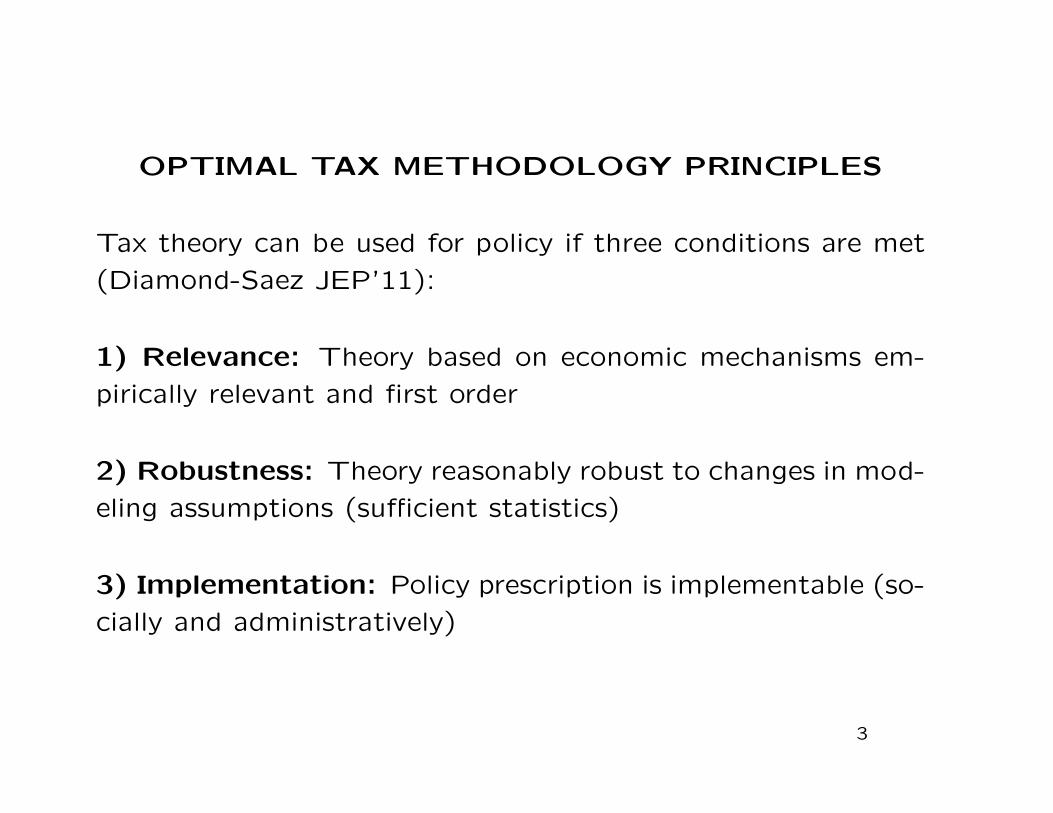
OPTIMAL TAX METHODOLOGY PRINCIPLES
Tax theory can be used for policy if three conditions are met
(Diamond-Saez JEP’11):
1) Relevance: Theory based on economic mechanisms em-
pirically relevant and first order
2) Robustness: Theory reasonably robust to changes in mod-
eling assumptions (sufficient statistics)
3) Implementation: Policy prescription is implementable (so-
cially and administratively)
3

OUTLINE OF CHAPTER
1) Historical and International Background on Taxes/Transfersand Policy Debate
2) Social Welfare and Labor Supply Concepts
3) Optimal Linear Income Tax
4) Optimal Nonlinear Income Tax: (a) Top earners, (b) Gen-eral profile, (c) Means-tested transfers
5) Extensions: (a) tax avoidance/evasion and income shifting,(b) trickle-up/down, (c) commodity taxation, (d) migration,(e) relative income concerns, (f) couples and children
6) Limitations: (a) utilitarian normative approach, (b) empir-ical evidence
4

2. SOCIAL WELFARE APPROACH
Individual i choose earnings z to maximize utility taking taxsystem into account
maxc,z
ui(c, z) s.t. c = z − T (z)
⇒ Taxes and transfers distort labor supply choices zi
Government maximizes a social welfare function s.t. to budget∫iG(ui)dν(i) s.t.
∫iT (zi)dν(i) ≥ E (p)
Social marginal welfare weight gi = G′(ui)uic/p measures thesocial value of giving $1 to person i (in terms of public funds)
Absent behavioral responses, the govt wants to redistribute tofully equalize the gi across individuals
T (z) includes both transfers (T (z) < 0 at bottom) and taxes(T (z) > 0 at top)
5

Effects of Taxes and Transfers Disposable
Incomec=z-T(z)
Market income z
45o Line: Budget with No taxes / transfers
G
0
Budget with taxes and transfers

3. OPTIMAL LINEAR TAX
c = (1 − τ) · z + R with τ linear tax rate and R demogrant
funded by taxes τZ with Z aggregate earnings
Individual labor supply choices zi(1− τ, R) aggregate to econ-
omy wide earnings Z(1− τ) =∫i zidν(i)
τ → τZ(1 − τ) is the “Laffer Curve” with top τ∗ = 1/(1 + e)
where e is the aggregate elasticity of Z wrt 1− τ
Optimal linear tax rate is:
τ =1− g
1− g + ewith g =
∫gizidν(i)∫
gidν(i) ·∫zidν(i)
< 1
captures the equity-efficiency trade-off robustly (τ ↓ g, τ ↓ e)
7

4. NON-LINEAR TAX: TOP EARNERS
Pre-tax top US incomes have surged in recent decades: top
1% income share increased from 9% in 1970 to 23.5% in 2007
(Piketty-Saez, 2003)
⇒ US Top 1% has huge potential fiscal capacity:
Absent behavioral responses, increasing Federal individual av-
erage tax rate on top 1% from current 22% to 43% would
raise revenue by 3 pts of GDP [$450bn/year]
Suppose top marginal tax rate is τ and applies above z∗ (in
US, τ = 42.5% including all taxes and z∗ = $400K ' top 1%
threshold)
8
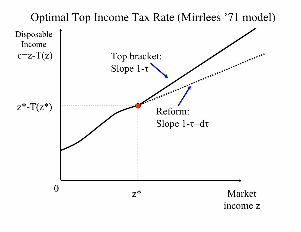
Optimal Top Income Tax Rate (Mirrlees ’71 model)Disposable
Incomec=z-T(z)
Market income z
Top bracket: Slope 1-τ
z*0
Reform: Slope 1-τ−dτ
z*-T(z*)

Disposable Income
c=z-T(z)
Market income z
z*
z*-T(z*)
0
Optimal Top Income Tax Rate (Mirrlees ’71 model)
Mechanical tax increase:dτ[z-z*]
Behavioral Response tax loss: τ dz = - dτ e z τ/(1-τ)
z

4. OPTIMAL TOP INCOME TAX RATE
Revenue maximizing top marginal tax rate (above z∗):
τ∗ =1
1 + a · ewhere e is the elasticity of top incomes with respect to 1− τ
and a = zm/(zm− z∗) is Pareto parameter with zm = average
income above z∗
a very stable with z∗ (around 1.5 today in the US)
If social weights gi converge to zero when z → ∞ ⇒ optimal
asymptotic tax rate is τ∗ = 1/(1 + a · e)
10

11.
52
2.5
Em
piric
al P
aret
o C
oeffi
cien
t
0 200000 400000 600000 800000 1000000z* = Adjusted Gross Income (current 2005 $)
a=zm/(zm-z*) with zm=E(z|z>z*) alpha=z*h(z*)/(1-H(z*))

4. ZERO TOP RATE RELEVANCE
Actual income distribution is finite and zm = z∗ at the top so
that a = zm/(zm − z∗) =∞ and τ∗ = 0 at the top. However:
1) Result applies only to highest earner (and not second high-
est)
2) Govt does not know top ex-ante: top income tail is a like
a finite draw from a Pareto distribution
If govt maximizes expected social welfare using an expected
revenue budget constraint then τ∗ = 1/(1 + a · e) remains the
optimal tax rate (Diamond-Saez JEP’11)
12

4. REAL VS. AVOIDANCE RESPONSES: THEORY
Fraction s of response dz to dτ due to avoidance (fraction 1−sis real) and “shifted income” s · dz is taxed at rate t ≤ τ
⇒ Tax revenue maximizing rate is (Saez, Slemrod, Giertz ’11)
τ =1 + a · t · s · e
1 + a · e1) If t = 0 then τ = 1/(1 +a ·e) (avoidance vs. real irrelevant)
2) If t > 0 then τ > 1/(1 + a · e) because of “fiscal externality”
3) Fully optimal policy: t = τ and τ = 1/[1 + a · (1 − s)e]with (1− s)e real elasticity (avoidance response s · e irrelevant)
⇒ (a) broaden the base and close loopholes, (b) then increase
top rates
13

4. RENT-SEEKING RESPONSES: THEORY
In models with frictions or imperfect information, pay z does
not always equal marginal product y ⇒ scope for rent-seeking
bargaining ⇒ Classical Externality
Suppose fraction s of the response dz to dτ is due to bargaining
(and fraction 1− s is real so that dy = (1− s)dz)
Tax revenue maximizing rate (Piketty, Saez, Stantcheva ’11):
τ =1 + a · s · e
1 + a · e1) Trickle-up: If top earners overpaid y < z, then s > 0 and
τ > 1/(1 + a · e)
2) Trickle-down: If top earners underpaid, then s < 0 is
possible and τ < 1/(1 + a · e)14

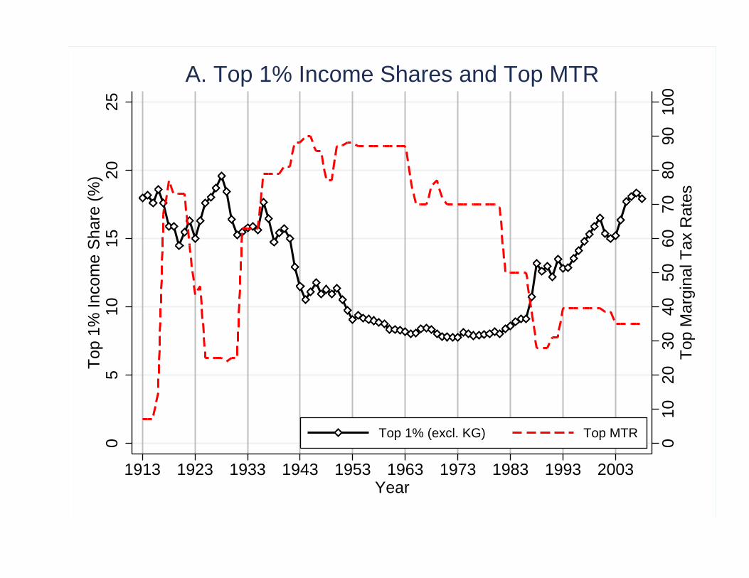
4. WHAT IS THE ELASTICITY FOR TOP
EARNERS?
Large empirical literature estimating e using tax reforms andmicro tax return data and aggregate share data
1) Long-run: Clear correlation between top income sharesand net-of-tax top rates in the long-run (within country andacross countries)
2) Short-run: Heterogeneity in size of behavioral responsesin the short-run
a) Large responses always due to tax avoidance (income shift-ing, income re-timing)
b) No compelling evidence of large real responses in the short-run
15
010
2030
4050
6070
8090
100
Top
Mar
gina
l Tax
Rat
es
05
1015
2025
Top
1%
Inco
me
Sha
re (
%)
1913 1923 1933 1943 1953 1963 1973 1983 1993 2003Year
Top 1% (excl. KG) Top MTR
A. Top 1% Income Shares and Top MTR
010
2030
4050
6070
8090
100
Mar
gina
l Tax
Rat
es (
%)
05
1015
2025
Top
1%
Inco
me
Sha
res
(%)
1913 1923 1933 1943 1953 1963 1973 1983 1993 2003Year
Top 1% (excl. KG) MTR K gains
Top 1% Share (incl. KG) Top MTR
B. Top 1% Income Shares and Top MTR
010
2030
4050
6070
8090
100
Mar
gina
l Tax
Rat
e (%
)
010
020
030
040
050
0R
eal I
ncom
e pe
r ad
ult (
1913
=10
0)
1913 1923 1933 1943 1953 1963 1973 1983 1993 2003Year
Top 1% Top MTR
Bottom 99%
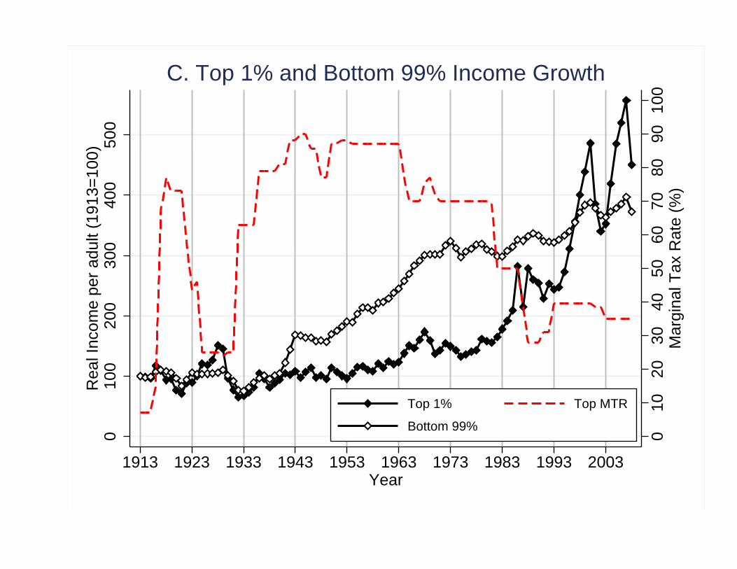
C. Top 1% and Bottom 99% Income Growth

AustraliaAustraliaAustraliaAustraliaAustraliaAustraliaAustraliaAustraliaAustraliaAustraliaAustraliaAustraliaAustraliaAustraliaAustraliaAustraliaAustraliaAustraliaAustraliaAustraliaAustraliaAustraliaAustraliaAustraliaAustraliaAustraliaAustraliaAustraliaAustraliaAustraliaAustraliaAustraliaAustralia
CanadaCanadaCanadaCanadaCanadaCanadaCanadaCanadaCanadaCanadaCanadaCanadaCanadaCanadaCanadaCanadaCanadaCanadaCanadaCanadaCanadaCanadaCanadaCanadaCanadaCanada
DenmarkDenmarkDenmarkDenmarkDenmarkDenmarkDenmarkDenmarkDenmarkDenmarkDenmarkDenmarkDenmarkDenmarkDenmarkDenmarkDenmarkDenmarkDenmarkDenmarkDenmarkDenmarkDenmarkDenmarkDenmarkDenmark
FinlandFinlandFinlandFinlandFinlandFinlandFinlandFinlandFinlandFinlandFinlandFinlandFinlandFinlandFinlandFinlandFinlandFinlandFinlandFinlandFinlandFinlandFinlandFinlandFinlandFinlandFinlandFinlandFinlandFinland
FranceFranceFranceFranceFranceFranceFranceFranceFranceFranceFranceFranceFranceFranceFranceFranceFranceFranceFranceFranceFranceFranceFranceFranceFranceFranceFranceFranceFranceFranceFranceFrance
GermanyGermanyGermanyGermanyGermanyGermanyGermanyGermanyGermanyGermanyGermanyGermanyGermanyGermanyGermanyGermanyGermanyGermanyGermanyGermanyGermanyGermanyGermanyGermany
IrelandIrelandIrelandIrelandIrelandIrelandIrelandIrelandIrelandIrelandIrelandIrelandIrelandIrelandIrelandIrelandIrelandIrelandIrelandIrelandIrelandIrelandIrelandIrelandIrelandIrelandItalyItalyItalyItalyItalyItalyItalyItalyItalyItalyItalyItalyItalyItalyItalyItalyItalyItalyItalyItalyItalyItalyItalyItalyItalyItalyItalyItaly JapanJapanJapanJapanJapanJapanJapanJapanJapanJapanJapanJapanJapanJapanJapanJapanJapanJapanJapanJapanJapanJapanJapanJapanJapanJapanJapanJapanJapanJapanJapan
NetherlandsNetherlandsNetherlandsNetherlandsNetherlandsNetherlandsNetherlandsNetherlandsNetherlandsNetherlandsNetherlandsNetherlandsNetherlandsNetherlandsNetherlandsNetherlandsNetherlandsNetherlandsNetherlandsNetherlandsNetherlandsNetherlandsNetherlandsNetherlandsNetherlandsNZNZNZNZNZNZNZNZNZNZNZNZNZNZNZNZNZNZNZNZNZNZNZNZNZNZNZNZNZNZNZ
NorwayNorwayNorwayNorwayNorwayNorwayNorwayNorwayNorwayNorwayNorwayNorwayNorwayNorwayNorwayNorwayNorwayNorwayNorwayNorwayNorwayNorwayNorwayNorwayNorwayNorwayNorwayNorwayNorwayNorwayNorwayNorwayNorwayNorwayPortugalPortugalPortugalPortugalPortugalPortugalPortugalPortugalPortugalPortugalPortugalPortugalPortugalPortugalPortugalPortugalPortugalPortugalPortugalPortugalPortugalPortugalPortugalPortugal
SpainSpainSpainSpainSpainSpainSpainSpainSpainSpainSpainSpainSpainSpainSpainSpainSpainSpainSpainSpainSpainSpainSpainSpainSpainSpainSpainSpain
SwedenSwedenSwedenSwedenSwedenSwedenSwedenSwedenSwedenSwedenSwedenSwedenSwedenSwedenSwedenSwedenSwedenSwedenSwedenSwedenSwedenSwedenSwedenSwedenSwedenSwedenSwedenSwedenSwedenSwedenSwedenSwedenSwedenSwedenSweden
SwitzerlandSwitzerlandSwitzerlandSwitzerlandSwitzerlandSwitzerlandSwitzerlandSwitzerlandSwitzerlandSwitzerlandSwitzerlandSwitzerlandSwitzerlandSwitzerlandSwitzerlandSwitzerlandSwitzerlandSwitzerlandSwitzerlandSwitzerlandSwitzerland
UKUKUKUKUKUKUKUKUKUKUKUKUKUKUKUKUKUKUKUKUKUKUKUKUKUKUKUKUKUK
USUSUSUSUSUSUSUSUSUSUSUSUSUSUSUSUSUSUSUSUSUSUSUSUSUSUSUSUSUSUSUSUSUS
46
810
1214
1618
Top
1%
Inco
me
Sha
re (
%)
40 50 60 70 80 90Top Marginal Tax Rate (%)
A. Top 1% Share and Top Marginal Tax Rate in 1975−9

AustraliaAustraliaAustraliaAustraliaAustraliaAustraliaAustraliaAustraliaAustraliaAustraliaAustraliaAustraliaAustraliaAustraliaAustraliaAustraliaAustraliaAustraliaAustraliaAustraliaAustraliaAustraliaAustraliaAustraliaAustraliaAustraliaAustraliaAustraliaAustraliaAustraliaAustraliaAustraliaAustralia
CanadaCanadaCanadaCanadaCanadaCanadaCanadaCanadaCanadaCanadaCanadaCanadaCanadaCanadaCanadaCanadaCanadaCanadaCanadaCanadaCanadaCanadaCanadaCanadaCanadaCanada
DenmarkDenmarkDenmarkDenmarkDenmarkDenmarkDenmarkDenmarkDenmarkDenmarkDenmarkDenmarkDenmarkDenmarkDenmarkDenmarkDenmarkDenmarkDenmarkDenmarkDenmarkDenmarkDenmarkDenmarkDenmarkDenmark
FinlandFinlandFinlandFinlandFinlandFinlandFinlandFinlandFinlandFinlandFinlandFinlandFinlandFinlandFinlandFinlandFinlandFinlandFinlandFinlandFinlandFinlandFinlandFinlandFinlandFinlandFinlandFinlandFinlandFinlandFranceFranceFranceFranceFranceFranceFranceFranceFranceFranceFranceFranceFranceFranceFranceFranceFranceFranceFranceFranceFranceFranceFranceFranceFranceFranceFranceFranceFranceFranceFranceFrance
GermanyGermanyGermanyGermanyGermanyGermanyGermanyGermanyGermanyGermanyGermanyGermanyGermanyGermanyGermanyGermanyGermanyGermanyGermanyGermanyGermanyGermanyGermanyGermanyIrelandIrelandIrelandIrelandIrelandIrelandIrelandIrelandIrelandIrelandIrelandIrelandIrelandIrelandIrelandIrelandIrelandIrelandIrelandIrelandIrelandIrelandIrelandIrelandIrelandIrelandItalyItalyItalyItalyItalyItalyItalyItalyItalyItalyItalyItalyItalyItalyItalyItalyItalyItalyItalyItalyItalyItalyItalyItalyItalyItalyItalyItaly
JapanJapanJapanJapanJapanJapanJapanJapanJapanJapanJapanJapanJapanJapanJapanJapanJapanJapanJapanJapanJapanJapanJapanJapanJapanJapanJapanJapanJapanJapanJapan
NetherlandsNetherlandsNetherlandsNetherlandsNetherlandsNetherlandsNetherlandsNetherlandsNetherlandsNetherlandsNetherlandsNetherlandsNetherlandsNetherlandsNetherlandsNetherlandsNetherlandsNetherlandsNetherlandsNetherlandsNetherlandsNetherlandsNetherlandsNetherlandsNetherlands
NZNZNZNZNZNZNZNZNZNZNZNZNZNZNZNZNZNZNZNZNZNZNZNZNZNZNZNZNZNZNZ
NorwayNorwayNorwayNorwayNorwayNorwayNorwayNorwayNorwayNorwayNorwayNorwayNorwayNorwayNorwayNorwayNorwayNorwayNorwayNorwayNorwayNorwayNorwayNorwayNorwayNorwayNorwayNorwayNorwayNorwayNorwayNorwayNorwayNorway
PortugalPortugalPortugalPortugalPortugalPortugalPortugalPortugalPortugalPortugalPortugalPortugalPortugalPortugalPortugalPortugalPortugalPortugalPortugalPortugalPortugalPortugalPortugalPortugal
SpainSpainSpainSpainSpainSpainSpainSpainSpainSpainSpainSpainSpainSpainSpainSpainSpainSpainSpainSpainSpainSpainSpainSpainSpainSpainSpainSpain
SwedenSwedenSwedenSwedenSwedenSwedenSwedenSwedenSwedenSwedenSwedenSwedenSwedenSwedenSwedenSwedenSwedenSwedenSwedenSwedenSwedenSwedenSwedenSwedenSwedenSwedenSwedenSwedenSwedenSwedenSwedenSwedenSwedenSwedenSweden
SwitzerlandSwitzerlandSwitzerlandSwitzerlandSwitzerlandSwitzerlandSwitzerlandSwitzerlandSwitzerlandSwitzerlandSwitzerlandSwitzerlandSwitzerlandSwitzerlandSwitzerlandSwitzerlandSwitzerlandSwitzerlandSwitzerlandSwitzerlandSwitzerland
UKUKUKUKUKUKUKUKUKUKUKUKUKUKUKUKUKUKUKUKUKUKUKUKUKUKUKUKUKUK
USUSUSUSUSUSUSUSUSUSUSUSUSUSUSUSUSUSUSUSUSUSUSUSUSUSUSUSUSUSUSUSUSUS4
68
1012
1416
18T
op 1
% In
com
e S
hare
(%
)
40 50 60 70 80 90Top Marginal Tax Rate (%)
B. Top 1% Share and Top Marginal Tax Rate in 2004−8

AustraliaAustraliaAustraliaAustraliaAustraliaAustraliaAustraliaAustraliaAustraliaAustraliaAustraliaAustraliaAustraliaAustraliaAustraliaAustraliaAustraliaAustraliaAustraliaAustraliaAustraliaAustraliaAustraliaAustraliaAustraliaAustraliaAustraliaAustraliaAustraliaAustraliaAustraliaAustraliaAustraliaCanadaCanadaCanadaCanadaCanadaCanadaCanadaCanadaCanadaCanadaCanadaCanadaCanadaCanadaCanadaCanadaCanadaCanadaCanadaCanadaCanadaCanadaCanadaCanadaCanadaCanada
DenmarkDenmarkDenmarkDenmarkDenmarkDenmarkDenmarkDenmarkDenmarkDenmarkDenmarkDenmarkDenmarkDenmarkDenmarkDenmarkDenmarkDenmarkDenmarkDenmarkDenmarkDenmarkDenmarkDenmarkDenmarkDenmark
FinlandFinlandFinlandFinlandFinlandFinlandFinlandFinlandFinlandFinlandFinlandFinlandFinlandFinlandFinlandFinlandFinlandFinlandFinlandFinlandFinlandFinlandFinlandFinlandFinlandFinlandFinlandFinlandFinlandFinland
FranceFranceFranceFranceFranceFranceFranceFranceFranceFranceFranceFranceFranceFranceFranceFranceFranceFranceFranceFranceFranceFranceFranceFranceFranceFranceFranceFranceFranceFranceFranceFrance
GermanyGermanyGermanyGermanyGermanyGermanyGermanyGermanyGermanyGermanyGermanyGermanyGermanyGermanyGermanyGermanyGermanyGermanyGermanyGermanyGermanyGermanyGermanyGermany
IrelandIrelandIrelandIrelandIrelandIrelandIrelandIrelandIrelandIrelandIrelandIrelandIrelandIrelandIrelandIrelandIrelandIrelandIrelandIrelandIrelandIrelandIrelandIrelandIrelandIreland
ItalyItalyItalyItalyItalyItalyItalyItalyItalyItalyItalyItalyItalyItalyItalyItalyItalyItalyItalyItalyItalyItalyItalyItalyItalyItalyItalyItalyJapanJapanJapanJapanJapanJapanJapanJapanJapanJapanJapanJapanJapanJapanJapanJapanJapanJapanJapanJapanJapanJapanJapanJapanJapanJapanJapanJapanJapanJapanJapan
NetherlandsNetherlandsNetherlandsNetherlandsNetherlandsNetherlandsNetherlandsNetherlandsNetherlandsNetherlandsNetherlandsNetherlandsNetherlandsNetherlandsNetherlandsNetherlandsNetherlandsNetherlandsNetherlandsNetherlandsNetherlandsNetherlandsNetherlandsNetherlandsNetherlands
NZNZNZNZNZNZNZNZNZNZNZNZNZNZNZNZNZNZNZNZNZNZNZNZNZNZNZNZNZNZNZ
NorwayNorwayNorwayNorwayNorwayNorwayNorwayNorwayNorwayNorwayNorwayNorwayNorwayNorwayNorwayNorwayNorwayNorwayNorwayNorwayNorwayNorwayNorwayNorwayNorwayNorwayNorwayNorwayNorwayNorwayNorwayNorwayNorwayNorway
PortugalPortugalPortugalPortugalPortugalPortugalPortugalPortugalPortugalPortugalPortugalPortugalPortugalPortugalPortugalPortugalPortugalPortugalPortugalPortugalPortugalPortugalPortugalPortugal
SpainSpainSpainSpainSpainSpainSpainSpainSpainSpainSpainSpainSpainSpainSpainSpainSpainSpainSpainSpainSpainSpainSpainSpainSpainSpainSpainSpain
SwedenSwedenSwedenSwedenSwedenSwedenSwedenSwedenSwedenSwedenSwedenSwedenSwedenSwedenSwedenSwedenSwedenSwedenSwedenSwedenSwedenSwedenSwedenSwedenSwedenSwedenSwedenSwedenSwedenSwedenSwedenSwedenSwedenSwedenSweden
SwitzerlandSwitzerlandSwitzerlandSwitzerlandSwitzerlandSwitzerlandSwitzerlandSwitzerlandSwitzerlandSwitzerlandSwitzerlandSwitzerlandSwitzerlandSwitzerlandSwitzerlandSwitzerlandSwitzerlandSwitzerlandSwitzerlandSwitzerlandSwitzerland
UKUKUKUKUKUKUKUKUKUKUKUKUKUKUKUKUKUKUKUKUKUKUKUKUKUKUKUKUKUK
USUSUSUSUSUSUSUSUSUSUSUSUSUSUSUSUSUSUSUSUSUSUSUSUSUSUSUSUSUSUSUSUSUS0
24
68
10C
hang
e in
Top
1%
Inco
me
Sha
re (
poin
ts)
−40 −30 −20 −10 0 10Change in Top Marginal Tax Rate (points)
A. Changes Top 1% Share and Top Marginal Tax Rate

AustraliaAustraliaAustraliaAustraliaAustraliaAustraliaAustraliaAustraliaAustraliaAustraliaAustraliaAustraliaAustraliaAustraliaAustraliaAustraliaAustraliaAustraliaAustraliaAustraliaAustraliaAustraliaAustraliaAustraliaAustraliaAustraliaAustraliaAustraliaAustraliaAustraliaAustraliaAustraliaAustralia
CanadaCanadaCanadaCanadaCanadaCanadaCanadaCanadaCanadaCanadaCanadaCanadaCanadaCanadaCanadaCanadaCanadaCanadaCanadaCanadaCanadaCanadaCanadaCanadaCanadaCanada
DenmarkDenmarkDenmarkDenmarkDenmarkDenmarkDenmarkDenmarkDenmarkDenmarkDenmarkDenmarkDenmarkDenmarkDenmarkDenmarkDenmarkDenmarkDenmarkDenmarkDenmarkDenmarkDenmarkDenmarkDenmarkDenmark
FinlandFinlandFinlandFinlandFinlandFinlandFinlandFinlandFinlandFinlandFinlandFinlandFinlandFinlandFinlandFinlandFinlandFinlandFinlandFinlandFinlandFinlandFinlandFinlandFinlandFinlandFinlandFinlandFinlandFinland
FranceFranceFranceFranceFranceFranceFranceFranceFranceFranceFranceFranceFranceFranceFranceFranceFranceFranceFranceFranceFranceFranceFranceFranceFranceFranceFranceFranceFranceFranceFranceFrance
GermanyGermanyGermanyGermanyGermanyGermanyGermanyGermanyGermanyGermanyGermanyGermanyGermanyGermanyGermanyGermanyGermanyGermanyGermanyGermanyGermanyGermanyGermanyGermany
IrelandIrelandIrelandIrelandIrelandIrelandIrelandIrelandIrelandIrelandIrelandIrelandIrelandIrelandIrelandIrelandIrelandIrelandIrelandIrelandIrelandIrelandIrelandIrelandIrelandIreland
ItalyItalyItalyItalyItalyItalyItalyItalyItalyItalyItalyItalyItalyItalyItalyItalyItalyItalyItalyItalyItalyItalyItalyItalyItalyItalyItalyItaly
JapanJapanJapanJapanJapanJapanJapanJapanJapanJapanJapanJapanJapanJapanJapanJapanJapanJapanJapanJapanJapanJapanJapanJapanJapanJapanJapanJapanJapanJapanJapan
NetherlandsNetherlandsNetherlandsNetherlandsNetherlandsNetherlandsNetherlandsNetherlandsNetherlandsNetherlandsNetherlandsNetherlandsNetherlandsNetherlandsNetherlandsNetherlandsNetherlandsNetherlandsNetherlandsNetherlandsNetherlandsNetherlandsNetherlandsNetherlandsNetherlands
NZNZNZNZNZNZNZNZNZNZNZNZNZNZNZNZNZNZNZNZNZNZNZNZNZNZNZNZNZNZNZ
NorwayNorwayNorwayNorwayNorwayNorwayNorwayNorwayNorwayNorwayNorwayNorwayNorwayNorwayNorwayNorwayNorwayNorwayNorwayNorwayNorwayNorwayNorwayNorwayNorwayNorwayNorwayNorwayNorwayNorwayNorwayNorwayNorwayNorwayPortugalPortugalPortugalPortugalPortugalPortugalPortugalPortugalPortugalPortugalPortugalPortugalPortugalPortugalPortugalPortugalPortugalPortugalPortugalPortugalPortugalPortugalPortugalPortugal SpainSpainSpainSpainSpainSpainSpainSpainSpainSpainSpainSpainSpainSpainSpainSpainSpainSpainSpainSpainSpainSpainSpainSpainSpainSpainSpainSpain
SwedenSwedenSwedenSwedenSwedenSwedenSwedenSwedenSwedenSwedenSwedenSwedenSwedenSwedenSwedenSwedenSwedenSwedenSwedenSwedenSwedenSwedenSwedenSwedenSwedenSwedenSwedenSwedenSwedenSwedenSwedenSwedenSwedenSwedenSweden
SwitzerlandSwitzerlandSwitzerlandSwitzerlandSwitzerlandSwitzerlandSwitzerlandSwitzerlandSwitzerlandSwitzerlandSwitzerlandSwitzerlandSwitzerlandSwitzerlandSwitzerlandSwitzerlandSwitzerlandSwitzerlandSwitzerlandSwitzerlandSwitzerland
UKUKUKUKUKUKUKUKUKUKUKUKUKUKUKUKUKUKUKUKUKUKUKUKUKUKUKUKUKUK
USUSUSUSUSUSUSUSUSUSUSUSUSUSUSUSUSUSUSUSUSUSUSUSUSUSUSUSUSUSUSUSUSUS
12
34
GD
P p
er c
apita
rea
l ann
ual g
row
th (
%)
−40 −30 −20 −10 0 10Change in Top Marginal Tax Rate (points)
B. Growth and Change in Top Marginal Tax Rate

4. ANATOMY OF BEHAVIORAL RESPONSES
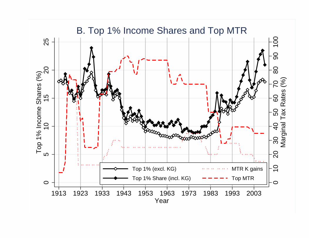
1) Avoidance: Is the surge in US top income shares ex-plained by reduced tax avoidance/evasion since 1970s insteadof change in real income?
Test: Under avoidance scenario, narrower measures of taxableincome should be much more responsive to marginal tax ratesthan broader measures including tax preferred income items
First pass is to compare income excluding and including taxpreferred realized capital gains ⇒ Does not support tax avoid-ance scenario
2) Rent-Seeking: Has top 1% income share surge come atthe expense of the 99%?
Test: First pass is to look at correlation between economicgrowth and top tax rate cuts⇒ No correlation supports trickle-up (more work needed)
16

4. INTERNATIONAL MIGRATION
Public debate concern that top skilled individuals move to lowtax countries (e.g., in EU context) or low tax states (withinUS Federation)
Optimal top tax rate with migration elasticity eM + intensiveelasticity e is:
τ =1
1 + a · e+ eM
Much less empirical work on eM (than on e)
Some EU countries have adopted special low flat tax schemesfor highly paid foreigners: Kleven et al. (2011) find enormousresponse with eM ≥ 1 in the case of Danish scheme
At global level eM = 0 ⇒ International cooperation increasestaxing power
17

Figure 3: Total number of foreigners in different income groups
01
00
02
00
03
00
04
00
0#
of
fore
ign
ers
19
80
19
81
19
82
19
83
19
84
19
85
19
86
19
87
19
88
19
89
19
90
19
91
19
92
19
93
19
94
19
95
19
96
19
97
19
98
19
99
20
00
20
01
20
02
20
03
20
04
20
05
20
06
20
07
20
08
Control 1 Control 2 Treatment
Control 1= annualized income between .8 and .9 of thresholdControl 2= annualized income between .9 and .995 of threshold.

4. GENERAL NONLINEAR OPTIMAL T ′(z)
Optimal tax formula T ′(z) [no income effects, Diamond AER’98]
T ′(z) =1−G(z)
1−G(z) + α(z) · e(z)
1) e(z) is elasticity at income level z
2) G(z) is the average social marginal welfare weight on indi-
viduals above z (G(z) ↓ z)
3) α(z) = zh(z)/[1 − H(z)] is the “local” Pareto parameter,
about constant in upper tail
e(z) constant ⇒ T ′(z) increases toward τ = 1/(1 + a · e)
19

Disposable Incomec=z-T(z)
Pre-tax income zz0
Mechanical tax increase: ddz [1-H(z)]Social welfare effect: -ddz [1-H(z)] G(z)
Behavioral response: z = - d e z/(1-T’(z))Tax loss: T’(z) z h(z)dz= -h(z) e z T’(z)/(1-T’(z)) dzd
z+dz
Small band (z,z+dz): slope 1- T’(z) Reform: slope 1- T’(z)d
ddz

11.
52
2.5
Em
piric
al P
aret
o C
oeffi
cien
t
0 200000 400000 600000 800000 1000000z* = Adjusted Gross Income (current 2005 $)
a=zm/(zm-z*) with zm=E(z|z>z*) alpha=z*h(z*)/(1-H(z*))
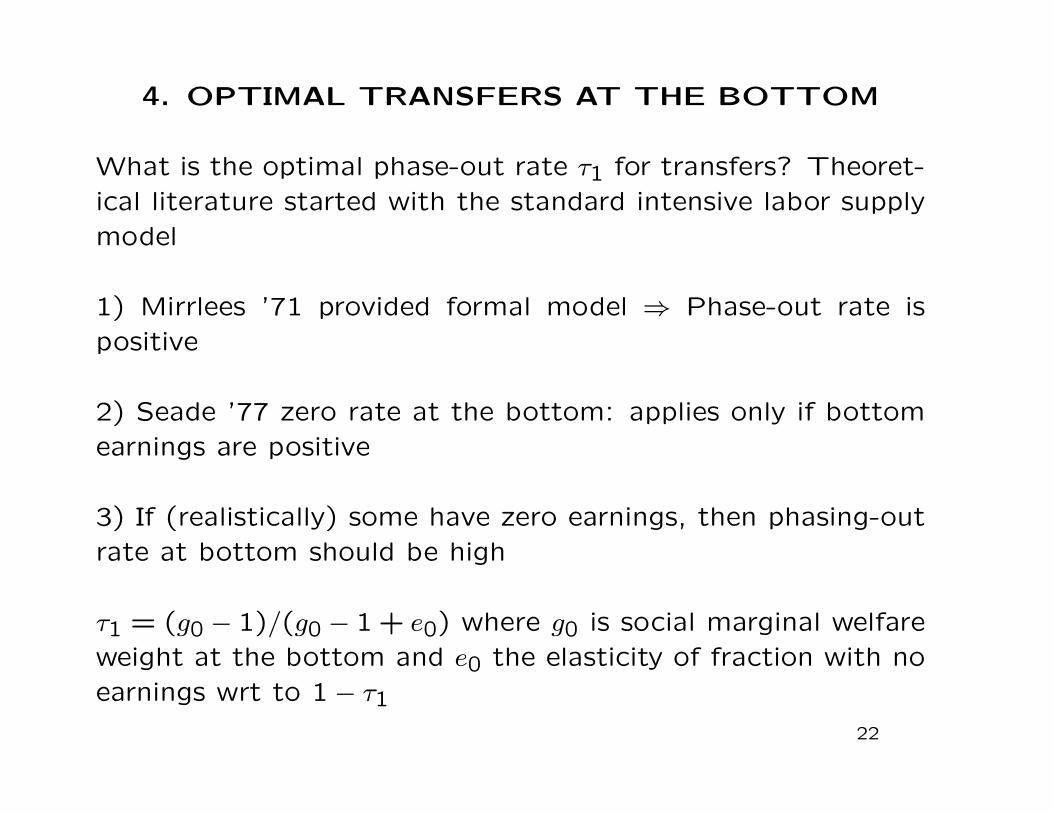
4. OPTIMAL TRANSFERS AT THE BOTTOM
What is the optimal phase-out rate τ1 for transfers? Theoret-ical literature started with the standard intensive labor supplymodel
1) Mirrlees ’71 provided formal model ⇒ Phase-out rate ispositive
2) Seade ’77 zero rate at the bottom: applies only if bottomearnings are positive
3) If (realistically) some have zero earnings, then phasing-outrate at bottom should be high
τ1 = (g0 − 1)/(g0 − 1 + e0) where g0 is social marginal welfareweight at the bottom and e0 the elasticity of fraction with noearnings wrt to 1− τ1
22

Disposable Income
c
Earnings z
45o
z1
c0
0
Reform: Increase 1 by d1 and c0 by dc0=z1d1
g0>>1 welfare effect >> mechanical fiscal cost
c0+dc0
Slope 1-1

Disposable Income
c
Earnings z
45o
z1
c0
0
Reform: Increase 1 by d1 and c0 by dc0=z1d1
g0>>1 welfare effect >> mechanical fiscal cost
Fiscal cost due to behavioral responses proportionalto 1/(1-1) and elasticity e0 =(1-1)/H0 dH0/d(1-1)
Optimal phase-out rate 1:1 = (g0-1)/(g0-1+ e0) Example: if g0=3 and e0=0.5, 1=80%
c0+dc0
Slope 1-1

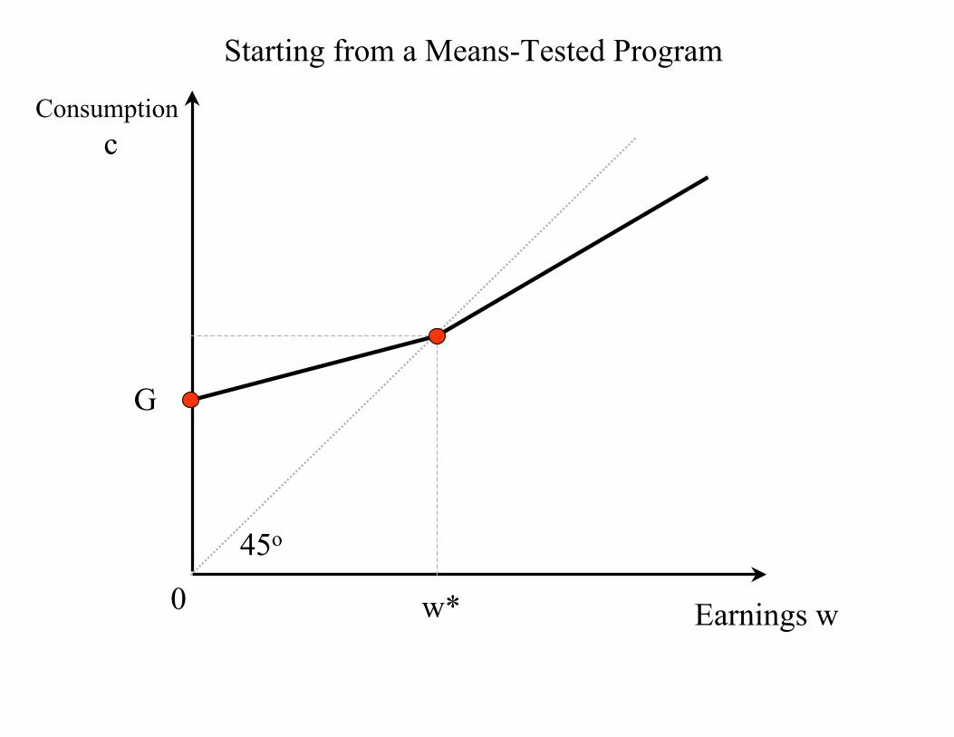
4. OPTIMAL TRANSFERS AT THE BOTTOM
Concern that high phase-out rate discourages labor force par-
ticipation rather than hours of work on the job [confirmed by
empirical studies over last 15-20 years]
Many countries have switched partly from traditional means-
tested transfers with high phase-out toward in-work benefits
(such as EITC in the US) to reward work
With extensive labor supply responses at the bottom, a neg-
ative phasing-out rate at the bottom (i.e., in-work benefit) is
optimal (Diamond ’80, Saez ’02)
⇒ Low earners should be subsidized on the margin
24
Starting from a Means-Tested Program
Consumptionc
Earnings w
45o
w*
G
0

Introducing a small EITC is desirable for redistributionConsumptionc
Earnings w
45o
w*
G
0
Starting from a Means-Tested Program

Introducing a small EITC is desirable for redistributionConsumptionc
Earnings w
45o
w*
G
0
Starting from a Means-Tested Program
Participation response saves government revenue

Introducing a small EITC is desirable for redistributionConsumptionc
Earnings w
45o
w*
G
0
Starting from a Means-Tested Program
Participation response saves government revenue
Win-Win reform

Introducing a small EITC is desirable for redistributionConsumptionc
Earnings w
45o
w*
G
0
Starting from a Means-Tested Program
Participation response saves government revenue
Win-Win reform If intensive response is small

NORMATIVE PUZZLES OF UTILITARIANISM
1) Too Little Tagging: Taxes and transfers should dependon all characteristics correlated with earnings potential (age,race, gender, height, education, family composition, etc.)
2) Fairness Perceptions: Utilitarian redistributive concernsare disconnected from process/behavior creating inequality. Inpractice, fairness perceptions of income process play criticalrole in views about taxes/transfers
3) Behavioral Biases: (a) Tax increases more painful thantax decreases, (b) Asymmetry between deserving taxpayers vs.transfer recipients, (c) Framing effects: taxes/transfer matterindividually not only the net T (z), (d) Relative income effects
Large literature in Social Choice develops alternative socialobjectives but tends to be very theoretical and optimal out-come sometimes Pareto dominated (Kaplow ’08, Fleurbaey’08 books)
26
ENDOGENOUS SOCIAL WELFARE WEIGHTS
A simple reduced form way to capture such non-standard ef-fects is to assume that social marginal welfare weights gi arenot derived from a standard SWF but determined endoge-nously by views and perceptions (Saez and Stantcheva 2011)
⇒ Standard optimal tax formulas as a function of the gi andthe behavioral elasticities continue to apply
⇒ Optimum no longer maximizes an objective but is an equi-librium: no small reform around the equilibrium is desirable
Wide latitude to set the gi to reflect social views, having thegi ≥ 0 guarantees a constrained Pareto efficient outcome
Future research: understand what shapes the gi endogenousweights
27

CONCLUSIONS
1) Recent literature has been successful in integrating theorywith empirical work
⇒ Provides a theory reasonably robust with clear economicintuitions that can be brought to data
2) Important limitations of both theory and empirical analysisremain
a) Empirical work: Relatively easy to measure responses oftaxable income but anatomy of the response (real, avoidance,rent-seeking) is hard to measure and yet critical for optimaltax
b) Theory: Utilitarianism has severe limitations. Need morefocus on how social preferences are shaped
28


