
Optimal Time-Consistent Monetary, Fiscal and DebtMaturity Policy∗
Eric M. Leeper† Campbell Leith‡ Ding Liu§
January 21, 2016
Abstract
We develop a New Keynesian model with government bonds of mixed matu-rity and solve for optimal time-consistent policy using global solution techniques.This reveals several non-linearities absent from LQ analyses with one-period debt.Firstly, the steady-state balances an inflation and debt stabilization bias to gener-ate a small negative debt value with a slight undershooting of the inflation target.This falls far short of first-best (‘war chest’) asset levels. Secondly, starting fromdebt levels consistent with currently observed debt to GDP ratios the optimal pol-icy will gradually reduce that debt, but the policy mix changes radically along thetransition path. At high debt levels there is a reliance on a relaxation of monetarypolicy to reduce debt through an expanded tax base and reduced debt service costs,while tax rates are used to moderate the increases in inflation. However, as debtlevels fall, the use of monetary policy in this way diminishes and the authority turnsto fiscal policy to continue debt reduction. This endogenous switch in the policymix occurs at higher debt levels, the longer the average debt maturity. Allowingthe policymaker to optimally vary debt maturity in response to shocks and acrossvarying levels of debt, we find that variations in maturity are largely used to sup-port changes in the underlying time-consistent policy mix rather than the speed offiscal correction. Finally, introducing a mild degree of policy maker myopia can re-produce steady-state debt to GDP ratios and inflation rates not dissimilar to thoseobserved empirically, without changing any of the qualitative results presented inthe paper.
Key words: New Keynesian Model; Government Debt; Monetary Policy; FiscalPolicy; Credibility; Time Consistency; Maturity Structure.
JEL codes: E62, E63
∗We are grateful for comments from Fabrice Collard, Wouter Den Haan as well as the audience atthe 21st Annual Conference on Computing in Economics and Finance, and the 30th Annual Congress ofthe European Economic Association. However, all errors remain our own.†Address: Department of Economics, Indiana University, Bloomington, IN 47405, U.S.A., Monash
University, and NBER. E-mail: [email protected].‡Address: Economics, Adam Smith Business School, West Quadrangle, Gilbert Scott Building, Uni-
versity of Glasgow, Glasgow G12 8QQ. E-mail: [email protected].§Address: Room 1001, Gezhi Building, School of Economics, Southwestern University of Finance and
Economics (Liulin Campus), 555, Liutai Avenue, Wenjiang District, Chengdu, Sichuan, P. R. China,611130. E-mail: [email protected]
1

1 Introduction
The recent global financial crisis has led to an unprecedented peacetime increase in gov-ernment debt in advanced economies. Figure 1 shows that the debt to GDP ratios inadvanced economies steadily increased from 73% in 2007 to 105.3% in 2014. This devel-opment has prompted an interest from both policy makers and researchers in rethinkingthe appropriate relationship among monetary policy, fiscal policy and debt managementpolicy. The conventional policy assignment calls upon monetary authorities to determinethe level of short-term interest rates in order to control demand and inflation, while thefiscal authorities choose the level of the budget deficit to ensure fiscal sustainability and adebt management office undertakes the technical issue of choosing the maturity and formin which federal debt is issued. With the onset of the 2007/2008 financial crisis and thesubsequent easing of monetary policy, the clean lines between these domains have blurred.With short-term interest rates at the zero lower bound, central banks have resorted toquantitative easing (QE) to support aggregate demand. Because QE shortens the matu-rity structure of debt instruments that private investors have to hold, central banks haveeffectively entered the domain of debt-management policy.1 At the same time, fiscal au-thorities’ debt-management offices have been extending the average maturity of the debtto mitigate fiscal risks associated with the government’s growing debt burden. Thesefiscal actions have operated as a kind of reverse quantitative easing, replacing money-likeshort-term debt with longer-term debt.2 The observation that monetary and fiscal poli-cies with regard to government debt have been pushing in opposite directions suggeststhe need to reconsider the principles underlying the optimal combination of monetary,fiscal and debt management policies.
Against this background, this paper studies jointly optimal monetary and fiscal policywhen the policy makers can issue a portfolio of bonds of multiple maturities, but cannotcommit. A major focus of the paper is on how the level and maturity of debt affectsthe optimal time-consistent policy mix and equilibrium outcomes in the presence of dis-tortionary taxes and sticky prices. From this analysis, we can draw some conclusionson questions like whether surprise inflation and interest rates are likely to be used, inaddition to adjustments to taxes and government spending, in order to reduce and stabi-lize debt. Given the magnitude of the required fiscal consolidation in so many advancedeconomies, how the policy mix is likely to change as debt is stabilized from these levelsis highly relevant.
In sticky price New Keynesian models with one-period government debt, Schmitt-Grohe and Uribe (2004b) show that even a mild degree of price stickiness implies nearlyconstant inflation and near random walk behavior in government debt and tax rates whenpolicy makers can commit to time-inconsistent monetary and fiscal policies, in responseto shocks. In other words, monetary policy should not be used to stabilize debt. However,Sims (2013) questions the robustness of this result when government can issue long-termnominal bonds. With only short-term government debt, unexpected current inflationor deflation is the only way to change its market value in cushioning fiscal shocks. Incontrast, if debt is long term, large changes in the value of debt can be achieved through
1The series of open market operations by the Federal Reserve between 2008 and 2014 and the expan-sion in excess reserves reduced the average duration of U.S. government liabilities by over 20%, from 4.6years to 3.6 years (Corhay et al., 2014)
2For instance, the stock of US government debt with a maturity over 5 years that is held by the public(excluding the holdings by the Federal Reserve) has risen from 8 percent of GDP at the end of 2007 to15 percent at the middle of 2014 (Greenwood et al., 2014).
2

sustained movements in the nominal interest rate, with much smaller changes in currentinflation. Based on these considerations, Sims sketches out a theoretical argument forusing nominal debt - of which the real value can be altered with surprise changes ininflation and interest rates - as a cushion against fiscal disturbances to substitute forlarge movements in distorting taxes. This mechanism is explored further in Leeper andLeith (2017).
Our paper contributes to the literature along at least three dimensions. Firstly, wetake both non-state-contingent short-term and long-term nominal bonds into account.The consideration of long-term debt and the maturity structure is motivated by Sims’theoretical insights as well as the empirical facts. Figure 2 (right panel) shows the averagedebt maturity in a selection of advanced countries is between 2 and 14 years. Moreover,in section 5.2.4, we extend our analysis to encompass a situation where the policy makercan optimally vary the maturity structure as part of the policy problem.
Secondly, we focus on the time-consistent policy problem which is less studied in theliterature, and allow for the possibility that the policy maker may suffer some degree of‘myopia’ as a means of capturing the frictions in fiscal policy making highlighted by thepolitical economy literature (see Alesina and Passalacqua (2017) for a recent survey of thepolitical economy of government debt). In contrast, Sims’ arguments for using surpriseinflation as a complement to tax adjustments were made in the context of an environ-ment where the policy-maker could commit. In a linear-quadratic approximation to thepolicy problem, Leith and Wren-Lewis (2013) show that the time inconsistency inherentin commitment policy means that the optimal time-consistent discretionary policy fordebt is quite different. The random walk result, typically, no longer holds, and insteaddebt returns to its steady-state level following shocks. In addition, time-consistent policyregime is arguably the more appropriate description of policymaking around the world.While the Ramsey policy implies it is optimal to induce a random walk in steady statedebt as a result of the standard tax smoothing argument, ex ante fiscal authorities typ-ically want to adopt fiscal rules which are actually quite aggressive in stabilizing debt.They then typically abandon these rules in the face of adverse shocks (see, for example,Calmfors and Wren-Lewis (2011) for details on the numerous breaches of the Stabilityand Growth Pact in Europe even prior to the financial crisis). There is, therefore, a clearfailure to adopt fiscal rules which mimic commitment policy. Understanding how optimaltime-consistent (possibly myopic) discretionary policy differs from its time-inconsistentcounterpart, in particular in its implications for debt dynamics, has particular empiri-cal relevance today as governments assess the extent to which they need to reverse thelarge increases in debt caused by the severe recession, in a context where fiscal policycommitments are often far from credible.
Thirdly, we solve the model non-linearly using the global solution methods which en-able us to analyze episodes with sharp increases in debt to GDP ratios as observed in manycountries during the global recession. Leith and Wren-Lewis (2013) adopt traditionallinear-quadratic (LQ) methods by using an artificial device to ensure the steady-state isefficient and then linearizing the model around this steady state, while Schmitt-Groheand Uribe (2004b) adopt a second-order approximation to the first-order conditions of theRamsey problem.3 In contrast, we are not imposing any kind of approximation around
3In LQ models with long-term debt, Leeper and Zhou (2013) ask some similar questions and theysolve the optimal monetary and fiscal policies from the timeless perspective, while Bhattarai et al. (2014)study optimal time-consistent monetary and fiscal policies, taking the zero lower bound constraint onnominal interest rate into consideration.
3

a steady-state so that we can fully explore the effects of non-linearities inherent in theNew Keynesian model.4 In fact, the results under discretion in Leith and Wren-Lewis(2013) suggest that there are massive non-linearities - for example, there is an overshoot-ing in the debt correction in a single period when the economy is linearized around highersteady state debt levels, but a more gradual debt reduction following shocks when thelinearization takes place around a lower debt to GDP ratio. This implies that the speedof debt stabilization is likely to be highly state dependent.
To address these non-linearities and the time-inconsistency problem which dependson the incentives to induce inflation surprises to stimulate the economy and/or deflatedebt, we develop a New Keynesian model augmented with fiscal policy and a portfolio ofmixed maturity bonds and solve the optimal time-consistent policy problem using globalnon-linear solution techniques. In particular, we study whether and how nominal govern-ment debt maturity affects optimal monetary and fiscal policy decisions and equilibriumoutcomes in the presence of distortionary taxes and sticky prices. In the model, the gov-ernment cannot commit, and would like to use unexpected inflation in two ways. Firstly,as implied by the usual inflation bias problem, the policy maker faces a temptation toboost inflation in order to stimulate an economy where production is sub-optimally lowdue to monopolistic competition and tax distortions. Since tax rates are endogenous inthe model, the extent of the inflationary bias problem is endogenous as well. Secondly,the policy maker faces a second bias in that surprise inflation can affect the real valueof the outstanding stock of nominal government liabilities. In this way, the governmentfaces the additional temptation to increase inflation in order to reduce its debt burden.Anticipating this, economic agents raise their inflationary expectations - following Leithand Wren-Lewis (2013) - we label this the ‘debt stabilization bias’. This bias is also statecontingent in that the efficacy of surprise inflation in stabilizing debt, and therefore thetemptation to resort to such a policy, is rising in the level of debt.
We find the following key results. Firstly, the steady-state balances the inflation anddebt stabilization biases to generate a small negative long-run optimal value for debt,which implies a slight undershooting of the inflation target in steady state. This fallsfar short of the accumulated level of assets that would be needed to finance governmentconsumption and eliminate tax and other distortions (the so-called ‘war chest’ level).
Secondly, starting from levels of debt consistent with currently observed debt to GDPratios, the optimal time-consistent policy will gradually reduce that debt, but with largeincreases in inflation and radical changes in the policy mix along the transition path. Athigh debt levels, there is a reliance on a relaxation of monetary policy to reduce debtthrough an expansion in the tax base and reduced debt service costs, while tax ratesare used to moderate the increases in inflation. However, as debt levels fall, the use ofmonetary policy in this way is diminished and the policy maker turns to fiscal policyto continue the reduction in debt. This is akin to a switch from an active to passivefiscal policy in rule based descriptions of policy, which occurs endogenously under theoptimal policy as debt levels fall. It can also be accompanied by a switch from passiveto active monetary policy. This switch in the policy mix occurs at higher debt levels,the longer the average maturity of government debt. The increase in inflation associatedwith the inflation and debt stabilization biases reduces bond prices. This means that for
4There are some recent papers using global solution techniques which consider optimal discretionarymonetary policy with trivial fiscal policy in the New Keynesian models, see Anderson et al. (2010),Van Zandweghe and Wolman (2011), Nakata (2013), Leith and Liu (2014), Ngo (2014) and amongothers.
4

a given deficit the policy maker will need to issue more bonds, but when debt is of longermaturity, the policy maker will also pay less to repay the existing debt stock. Therefore,with longer maturity debt the desire to reduce debt rapidly along the transition pathis reduced and the debt stabilization bias is mitigated. As a result, for a longer debtmaturity, ceteris paribus, the policy maker is freer to raise taxes to stabilize debt, as themarginal inflationary costs of such tax increases are lower.
Thirdly, we also consider how the time-consistent policy maker would vary debt ma-turity, in response to shocks and across varying levels of debt. We show that variationsin the maturity structure are optimally used to support alterations in the time-consistentpolicy mix, rather than support a significantly different speed of fiscal correction.
Finally, we allow for the possibility that the policy maker may by ‘myopic’ in thesense that they discount the future more heavily than the infinitely lived household, asa means of capturing the short-termism in policy making that may be induced by thepolitical process. We find that this can easily shift steady-state equilibrium debt levelsand deviations of inflation from target, from negative to positive in line with observedvalues, without qualitatively affecting the rest of our conclusions.
Related Literature: Our paper is related to several strands of the optimal mon-etary and fiscal policy literature. We will discuss those that are most closely related interms of topics and numerical methods.
Our contribution is most closely related to the literature that studies optimal fiscaland monetary policy in sticky price New Keynesian models using non-linear solution tech-niques. Following the work of Schmitt-Grohe and Uribe (2004b) and Siu (2004), Faragliaet al. (2013) solve a Ramsey problem using a parameterized expectation algorithm (PEA)to examine the implications for optimal inflation of changes in the level and maturity ofgovernment debt. We study the discretionary equivalent of this policy, which is radicallydifferent. Niemann and Pichler (2011) globally solve for optimal fiscal and monetarypolicies under both commitment and discretion in an economy exposed to large adverseshocks. Using the same projection method, Niemann et al. (2013) study time-consistentpolicy in the model of Schmitt-Grohe and Uribe (2004b) and identify a simple mechanismthat generates inflation persistence. Government spending is exogenous in the latter twopapers which also do not consider long-term debt. Similarly, abstracting from long-termdebt, Matveev (2014) compares the efficacy of discretionary government spending andlabor income taxes for the purpose of fiscal stimulus at the liquidity trap. The valuefunction iteration (VFI) method is adopted to deal with the zero lower bound problem.In contrast to these papers, debt of different maturities, time-consistent optimal policymaking and endogenous government expenditure are all essential elements in our model.
Aside from the relatively small literature exploring optimal monetary and fiscal pol-icy in non-linear New Keynesian models, there is a vast literature on Ramsey fiscal andmonetary policy in the tradition of Lucas and Stokey (1983), which tends to focus onreal or flexible-price economies. In flexible-price environments, the government’s prob-lem consists in financing an exogenous stream of public spending by choosing the leastdisruptive combination of inflation and distortionary income taxes. In an incomplete-markets version of Lucas and Stokey (1983), Aiyagari et al. (2002) simulate the modelglobally and show that the level of welfare in Ramsey economies with and without realstate-contingent debt is virtually the same. In addition, they reaffirm the random-walkresults of debt and taxes from Barro (1979). Angeletos et al. (2013) introduce collateralconstraints and a liquidity role for government bonds into Aiyagari et al. (2002). They use
5

the VFI method to globally solve the modified model and find that the steady-state levelof debt is no longer indeterminate, when government bonds can serve as collateral. Cao(2014) extends Angeletos et al. (2013) with long-term debt and studies how the cost ofinflation for commercial banks affects the design of fiscal and monetary policy. Likewise,Faraglia et al. (2014) use the PEA methods to solve a Ramsey problem with incompletemarkets and long-term bonds. They show that many features of optimal policy are sen-sitive to the introduction of long-term bonds, in particular tax variability and the longrun behavior of debt. Our findings convey the same message that maturity lengths likethose observed in actual economies can substantially alter the nature of optimal policies,but the policy problem in our sticky price economy where the policy maker is unable tocommit is fundamentally different.
There is also a literature on optimal fiscal and monetary policy in monetary models,which do not contain nominal interia, but may contain a cost to inflation. Schmitt-Grohe and Uribe (2004a) study Ramsey policy in a flexible-price model with cash-in-advance constraint, which essentially extends the model of Lucas and Stokey (1983) to animperfectly competitive environment. A global numerical method is used to characterizethe dynamic properties of the Ramsey allocation. In a cash-in advance model, Martin(2009) studies the time consistency problems that arise from the interaction betweendebt and monetary policy, since inflation reduces the real value of nominal liabilities. Heuses the projection methods to deal with the generalized Euler equations, see also Martin(2011), Martin (2013) and Martin (2014) where time consistent policies are studied invariants of the monetary search model of Lagos and Wright (2005). In contrast, weabstract from monetary frictions and emphasize nominal price stickiness which is theconventional approach to generating sizable real effects from monetary policy.
Moving away from models which jointly model monetary and fiscal policy, there isalso a literature on optimal time-consistent fiscal policy in real models. This literaturetypically focuses on Markov-perfect policy, where households’ and the government’s pol-icy rules are functions of payoff-relevant variables only. Local approximations around anon-stochastic steady state are typically infeasible for these models, since optimal behav-ior is characterized by generalized Euler equations that involve the derivatives of someequilibrium decision rules, and thus it is impossible to compute the steady state indepen-dent of these rules. Hence, as in our contribution, global solution methods are required.Klein and Rios-Rull (2003) compare the stochastic properties of optimal fiscal policywithout commitment with those properties under a full-commitment policy in a neoclas-sical growth model with a balanced government budget, see also Krusell et al. (2006)and Klein et al. (2008). Ortigueira (2006) studies Markov-perfect optimal taxation undera balanced-budget rule, while Ortigueira et al. (2012) deal with the case of unbalancedbudgets. In a version of Lucas and Stokey (1983) model with endogenous governmentexpenditure, Debortoli and Nunes (2013) find that when governments cannot commit,debt is no longer indeterminate and often converges to a steady-state with no debt accu-mulation at all. This is a quite striking difference in the behavior of debt between the fullcommitment and the no-commitment cases. Similarly, Grechyna (2013) also considersendogenous government spending in the environment of Lucas and Stokey (1983) withonly one-period debt and shows that around the steady state, the properties of the fiscalvariables are very similar, regardless of commitment assumptions. More recently, Debor-toli et al. (2015) consider a Lucas and Stokey (1983) economy without state-contingentbonds and commitment, and show that the government actively manages its debt posi-tions and can approximate optimal policy by confining its debt instruments to consols.
6

Our paper shares the same technical problem due to the presence of generalized Eulerequations, but nominal rigidities make our model setup quite different from these papers.
Finally, the new political economy literature (see Alesina and Passalacqua (2017) fora comprehensive survey) considers how various aspects of the political process affect theaccumulation of government debt, and the tendency of some economies to be prone toa deficit bias. While there are numerous mechanisms through which political economyconsiderations influence fiscal policy, including the use of debt as a strategic variable, warsof attrition over who bears the burden of fiscal reforms and the nature of the budgetaryprocess itself, in essence these political frictions imply that policy makers may not fullyinternalize the long-term benefits of lower debt, while remaining acutely aware of theshort-term costs of any fiscal correction. We shall capture this implicit myopia informally,by considering the implications of the policy maker discounting the future at a rate whichis higher than that of society as a whole.
Roadmap. The paper proceeds as follows. We describe the benchmark model insection 2. The first best allocations are characterized in section 3. We study the optimaltime consistent policy problem in section 4. In section 5, we describe the solution methodand present the numerical results. In section 6 we conclude.
2 The Model
Our model is a standard New Keynesian model, but augmented to include the govern-ment’s budget constraint where government spending is financed by distortionary tax-ation and/or borrowing. This basic set-up is similar to that in Benigno and Woodford(2003) and Schmitt-Grohe and Uribe (2004b), but with some differences. Firstly, we al-low the government to optimally vary government spending in the face of shocks, ratherthan simply treating government spending as an exogenous flow which must be financed.This is a necessary modification to consider issues like assessing the relative efficacy ofgovernment spending cuts and tax increases in debt stabilization.5 Secondly, our nominaldebt is not of single-period maturity, but consists of a portfolio of bonds of mixed maturi-ties. In reality, most countries issue long-term nominal debt in overwhelming proportionsof total debt. This is an important consideration in highly indebted economies, sinceeven modest surprise changes in inflation and interest rates can have substantial effectson the market value of debt, and hence become a meaningful source of fiscal revenue.6
This fact suggests that the maturity structure of debt is an essential element in charac-terizing jointly optimal monetary and fiscal policy. Thirdly, we not only take the averagedebt maturity as exogenously given, but also allow it to optimally vary over the businesscycle, see section C.3 in the appendix. Finally, we capture informally the implicationsof adding political frictions to the policy making process by assuming the policy maker’stime horizon may be shortened as a result of the electoral cycle.
5International Monetary Fund (2012) reports that current fiscal consolidation efforts rely heavily ongovernment spending cuts. In addition, Bi et al. (2013) introduce ex ante uncertainty over the compo-sition of the fiscal consolidation, either tax based or spending based, and show that the macroeconomicconsequences of spending cuts can be quite different from tax increases, even if the direct fiscal conse-quences are similar.
6See Hall and Sargent (2011) and Sims (2013) for the empirical findings on the contribution of thiskind of fiscal financing to the decline in the U.S. debt-GDP ratio from 1945 to 1974.
7
2.1 Households
There are a continuum of households of size one. Households appreciate private consump-tion as well as the provision of public goods and dislike labor. We shall assume completeasset markets, such that, through risk sharing, they will face the same budget constraint.As a result the typical household will seek to maximize the following objective function
E0
∞∑t=0
βtU (Ct, Nt, Gt) (1)
where C, G and N are a consumption aggregate, a public goods aggregate, and laboursupply respectively.
The consumption aggregate is defined as
Ct =
(∫ 1
0
Ct(j)ε−1ε dj
) εε−1
(2)
where j denotes the good’s type or variety and ε > 1 is the elasticity of substitutionbetween varieties. The public goods aggregate takes the same form
Gt =
(∫ 1
0
Gt(j)ε−1ε dj
) εε−1
(3)
The budget constraint at time t is given by∫ 1
0
Pt(j)Ct(j)dj + P St B
St + PM
t BMt ≤ Ξt + (1 + ρPM
t )BMt−1 +BS
t−1 +WtNt(1− τt)
where Pt(j) is the price of variety j , Ξ is the representative household’s share of profitsin the imperfectly competitive firms, W are wages, and τ is an wage income tax rate.7
Households hold two basic forms of government bond. The first is the familiar one perioddebt, BS
t which has the price equal to the inverse of the gross nominal interest rate,P St = R−1
t . The second type of bond, following Woodford (2001), is actually a portfolioof many bonds which pay a declining coupon of ρj dollars j + 1 periods after they wereissued, where 0 < ρ ≤ β−1. The duration of the bond is given by (1− βρ)−1, which allowsus to vary ρ as a means of changing the implicit maturity structure of government debt.By using such a simple structure, we need only price a single bond, since any existingbond issued j periods ago is worth ρj new bonds. In the special case where ρ = 1, thesebonds become infinitely lived consols, and when ρ = 0, the bonds reduce to the familiarsingle period bonds typically studied in the literature.
Households must first decide how to allocate a given level of expenditure across thevarious goods that are available. They do so by adjusting the share of a particular goodin their consumption bundle to exploit any relative price differences - this minimizes thecosts of consumption. Optimization of expenditure for any individual good implies the
7Since fiscal policy is one important element of this paper, we do not assume any kind of lump-sum-tax-financed subsidy to offset the distortion arising from monopolistic competition, which is a typicalassumption in the optimal fiscal and monetary policy literature using New Keynesian models. Thus, thesteady-state of the model economy need not be efficient. In addition, in the presence of the zero lowerbound constraint, policy functions have kinks, therefore an accurate evaluation of optimal policy andwelfare requires a global solution method.
8

demand function given below,
Ct(j) =
(Pt(j)
Pt
)−εCt
where we have price indices given by
Pt =
(∫ 1
0
Pt(j)1−εdj
) 11−ε
The budget constraint, therefore, can be rewritten as
P St B
St + PM
t BMt ≤ Ξt + (1 + ρPM
t )BMt−1 +BS
t−1 +WtNt(1− τt)− PtCt (4)
where∫ 1
0Pt(j)Ct(j)dj = PtCt. Pt is the current price level. The constraint says that
total financial wealth in period t can be worth no more than the value of financial wealthbrought into the period, plus nonfinancial income during the period net of taxes and thevalue of consumption spending.
For much of the analysis, the one period government bond BSt is assumed to be in zero
net supply with beginning-of-period price P St , while the general portfolio of government
bond BMt is in non-zero net supply with beginning-of-period price PM
t . Higher ρ raises thematurity of the bond portfolio. We cannot allow the rate of decay on bonds to becometime varying, without either implicitly allowing the government to renege on existingbond contracts or tracking the distribution of bonds of different maturities that havebeen issued in the past. Therefore, in order to allow the policy maker to tractably varythe maturity structure, we shall in section 5.2.4 consider the case where both BS
t andBMt are potentially in non-zero net supply, so that the policy maker can vary the overall
maturity of the outstanding debt stock by varying the relative proportion of short andlonger-term bonds in that portfolio.
Similarly, the allocation of government spending across goods is determined by min-imizing total costs,
∫ 1
0Pt(j)Gt(j)dj. Given the form of the basket of public goods, this
implies,
Gt(j) =
(Pt(j)
Pt
)−εGt
2.1.1 Households’ Intertemporal Consumption Problem
The first part of the households intertemporal problems involves allocating consumptionexpenditure across time. For tractability, assume that (1) takes the specific form
E0
∞∑t=0
βt
(C1−σt
1− σ+ χ
G1−σgt
1− σg− Nt
1+ϕ
1 + ϕ
)(5)
We can then maximize utility subject to the budget constraint (4) to obtain theoptimal allocation of consumption across time, based on the pricing of one period bonds,
βRtEt
(CtCt+1
)σ (PtPt+1
)= 1 (6)
9

and the declining payoff consols,
βEt
(CtCt+1
)σ (PtPt+1
)(1 + ρPM
t+1
)= PM
t (7)
Notice that when these reduce to single period bonds, ρ = 0, the price of these bondswill be given by PM
t = R−1t . However, outside of this special case, the longer term bonds
introduce the term structure of interest rates to the model. It is convenient to define thestochastic discount factor (for nominal payoffs) for later use,
β
(CtCt+1
)σ (PtPt+1
)= Qt,t+1
The second FOC relates to their labour supply decision and is given by,
(1− τt)(Wt
Pt
)= Nϕ
t Cσt
That is, the marginal rate of substitution between consumption and leisure equals theafter-tax wage rate. Besides these FOCs, necessary and sufficient conditions for house-hold optimization also require the households’ budget constraints to bind with equality.Defining household wealth brought into period t as,
Dt = (1 + ρPMt )BM
t−1 +BSt−1
the no-Ponzi-game condition can be written as,
limT→∞
Et
[1
Rt,T
DT
PT
]≥ 0 (8)
where
Rt,T =T−1∏s=t
(1 + ρPM
s+1
PMs
PsPs+1
)for T ≥ 1 and Rt,t = 1, also see Eusepi and Preston (2011). The no-Ponzi-game saysthat the present discounted value of household’s real wealth at infinity is non-negative,that is, there is no overaccumulation of debt. In equilibrium, the condition holds withequality.
2.2 Firms
The production function is linear, so for firm j
Yt(j) = AtNt(j) (9)
where at = ln(At) is AR(1) such that at = ρaat−1 + eat, with 0 ≤ ρa < 1 and eati.i.d∼
N(0, σ2a). The real marginal costs of production is defined as mct = Wt/ (PtAt). The
demand curve they face is given by,
Yt(j) =
(Pt(j)
Pt
)−εYt
10

where Yt =[∫ 1
0Yt(j)
ε−1ε dj
] εε−1
. Firms are also subject to quadratic adjustment costs in
changing prices, as in Rotemberg (1982).We define the Rotemberg price adjustment costs for a monopolistic firm j as,
vt (j) =φ
2
(Pt(j)
Π∗Pt−1(j)− 1
)2
Yt (10)
where φ ≥ 0 measures the degree of nominal price rigidity. The adjustment cost, whichaccounts for the negative effects of price changes on the customer–firm relationship, in-creases in magnitude with the size of the price change and with the overall scale ofeconomic activity Yt.
The problem facing firm j is to maximize the discounted value of profits,
maxPt(j)
Et
∞∑z=0
Qt,t+zΞt+z (j)
where profits are defined as,
Ξt(j) = Pt(j)Yt(j)−mctYt(j)Pt −φ
2
(Pt(j)
Π∗Pt−1(j)− 1
)2
PtYt
So that, in a symmetric equilibrium where Pt(j) = Pt the first order conditions are givenby,
0 = (1− ε) + εmct − φΠt
Π∗
(Πt
Π∗− 1
)(11)
+ φβEt
[(CtCt+1
)σYt+1
Yt
Πt+1
Π∗
(Πt+1
Π∗− 1
)]which is the Rotemberg version of the non-linear Phillips curve relationship.
2.2.1 Market Clearing
Goods market clearing requires, for each good j,
Yt(j) = Ct(j) +Gt(j) + vt(j)
which allows us to write,Yt = Ct +Gt + vt
with vt =∫ 1
0vt (j) dj. In a symmetrical equilibrium,
Yt
[1− φ
2
(Πt
Π∗− 1
)2]
= Ct +Gt
There is also market clearing in the bonds market where we assume, initially, that theone period bonds are in zero net supply, BS
t = 0 and the remaining longer term portfolioevolves according to the government’s budget constraint which we will now describe.
11

2.3 Government Budget Constraint
The government consists of two authorities. First, there is a monetary authority whichcontrols the nominal interest rates on short-term nominal bonds. Second, there is a fiscalauthority deciding on the level of government expenditures, labor income taxes and ondebt policy. Government expenditures consist of spending for the provision of publicgoods and for interest payments on outstanding debt. The level of public goods provisionis a choice variable of the government. We assume that monetary and fiscal policy iscoordinated by a benevolent policymaker who seeks to maximize household welfare, andthe government can credibly commit to repay its debt. We shall consider the implicationsof policy maker myopia motivated by political frictions in section 5.2.5.
Government expenditures Gt are financed by levying labor income taxes at the rateτt, and by issuing one-period, risk free (non-contingent), nominal obligations BS
t , andlong term bonds BM
t . The government’s sequential budget constraint is then given by
PMt BM
t + P St B
St + τtWtNt = PtGt +BS
t−1 + (1 + ρPMt )BM
t−1
Assuming that the one-period bond is assumed in zero net supply,8 that is, BSt = 0, and
rewriting in real terms
PMt bt = (1 + ρPM
t )bt−1
Πt
− Wt
PtNtτt +Gt (12)
where real debt is defined as, bt ≡ BMt /Pt.
Given the nominal nature of debt, monetary policy decisions affect the governmentbudget through three channels: first, the nominal interest rate policy of the monetaryauthority influences directly the nominal return the government has to offer on its in-struments; second, nominal interest rate decisions also affect the price level and therebythe real value of outstanding government deb; and third, in our sticky-price economy thereal effects of monetary policy can affect the size of the tax base.
In particular, the role of the maturity of government debt can be seen clearly from thegovernment budget constraint. In (12), the amount of outstanding real government debtis PM
t bt, and the period real return on holding government debt is (1 + ρPMt )/
(ΠtP
Mt−1
).
If ρ = 0, government debt bt is reduced to one-period debt, and the only way to adjustthe real return on bonds ex post is through inflation in the current period Πt. Largefluctuations in prices can be very costly in the presence of nominal rigidities. However,if government debt has a longer maturity, 0 < ρ < 1, adjustments in the ex post realreturn can be engineered via changes in the bond price PM
t , which depends on inflationin future periods. This means that changes in the real debt return can be produced bya small, but sustained inflation, which is less costly than equivalent large fluctuations incurrent inflation. As a result, long-term debt helps the policy maker achieve the desiredadjustment in the ex post real return at a smaller cost.
That completes the description of our model which consists of the usual resourceconstraint, consumption Euler equation and New Keynesian Phillips curve as well as thegovernment’s budget constraint and the bond pricing equation for longer-term bonds.These equations and the debt-dependent steady state are described in the Appendix C.1.
8We shall re-introduce short-term debt alongside longer-term debt in section 5 below.
12

3 First-Best Allocation
In some analyses of optimal fiscal policy (e.g., Aiyagari et al., 2002), it is desirable forthe policy maker to accumulate a ‘war chest’ which pays for government consumptionand/or fiscal subsidies to correct for other market imperfections. In order to assess towhat extent our optimal, but time-consistent policy attempts to do so, it is helpful todefine the level of government accumulated assets that would be necessary to mimic thesocial planner’s allocation under the decentralized solution. The first step in doing so isdefining the first-best allocation that would be implemented by the social planner. Thesocial planner ignores the nominal inertia and all other inefficiencies, and chooses realallocations that maximize the representative consumer’s utility, subject to the aggregateresource constraint and the aggregate production function. That is, the first-best allo-cation C∗t , N∗t , G∗t is the one that maximizes utility (36), subject to the technologyconstraint (35), and aggregate resource constraint Yt = Ct +Gt.
The first order conditions imply that
(C∗t )−σ = χ (G∗t )−σg = (Nt
∗)ϕ /At = (Yt∗)ϕA
−(1+ϕ)t
That is, given the resource constraints, it is optimal to equate the marginal utility ofprivate and public consumption to the marginal disutility of labor effort and the optimalshare of government consumption in output is
G∗tY ∗t
= χ1σg
(Yt∗
At
)−ϕ+σgσg
A1−σgσg
t
In steady state (technology level A normalized to unity) and assuming σ = σg, thisimplies the optimal share of government consumption in output is
G∗
Y ∗=(
1 + χ−1σ
)−1
and the first-best level of output is given by,
(Y ∗)ϕ+σ
(1− G∗
Y ∗
)σ= 1 (13)
It is illuminating to contrast the allocation achieved in the steady state of the decen-tralized equilibrium with this first best allocation. We do this by finding policies andprices that make the first-best allocation and the decentralized equilibrium coincide. Ap-pendix C.1 shows that the steady-state level of output in the decentralized economy isgiven by,
Y ϕ+σ
(1− G
Y
)σ= (1− τ)
(ε− 1
ε
)(14)
Comparing (14) and (13), and assuming the steady state share of government consump-tion is the same, then the two allocations will be identical when the labor income taxrate is set optimally to be,
τ ∗ = 1− ε
ε− 1=−1
ε− 1(15)
Notice that the optimal tax rate is negative, that is, it is effectively a subsidy which offsets
13

the monopolistic competition distortion. This, in turn, requires that the government hasaccumulated a stock of assets defined as,
PM∗b∗
4Y ∗=
β
4 (1− β)
[−1
ε−(
1 + χ−1σ
)−1]
Using our benchmark calibration below, this would imply that a stock of assets of 843.75%of GDP would be required to generate sufficient income to pay for government consump-tion and a labor income subsidy which completely offsets the effects of the monopolisticcompetition distortion. We shall see that the steady-state level of debt in our optimalpolicy problem while negative, falls far short of this ‘war chest’ value.
4 Optimal Policy Under Discretion
We assume that the policymaker cannot credibly commit to particular future policyactions. Instead, the policymaker reoptimizes his policy response each period, that is,this policy is time-consistent. In our model, the presence of government debt makes theoptimal time-consistent policy history dependent, in that the future path of the policyinstruments depends on today’s level of government debt.
The policy under discretion can be described as a set of decision rules for Ct, Yt,Πt, bt, τt, Gtwhich maximize,
V (bt−1, At) = max
C1−σt
1− σ+ χ
G1−σgt
1− σg− (Yt/At)
1+ϕ
1 + ϕ+ βEt [V (bt, At+1)]
subject to the resource constraint (32), the New Keynesian Phillips curve (33), and thegovernment’s budget constraint,
βEt
(CtCt+1
)σ (PtPt+1
)(1 + ρPM
t+1
)bt (16)
=
(1 + ρβEt
(CtCt+1
)σ (PtPt+1
)(1 + ρPM
t+1
)) bt−1
Πt
−(
τt1− τt
)(YtAt
)1+ϕ
Cσt +Gt
where we have used the bond pricing equation (31) to eliminate the current value of thebond in (34).
Defining auxiliary functions,
M(bt, At+1) = (Ct+1)−σ Yt+1Πt+1
Π∗
(Πt+1
Π∗− 1
)L(bt, At+1) = (Ct+1)−σ(Πt+1)−1(1 + ρPM
t+1)
we can write the constraints (33) and (16) facing the policy maker as,
(1− ε) + ε(1− τt)−1Y ϕt C
σt A−1−ϕt − φΠt
Π∗
(Πt
Π∗− 1
)+ φβCσ
t Y−1t Et [M(bt, At+1)] = 0 (17)
14

0 = βbtCσt Et [L(bt, At+1)]− bt−1
Πt
(1 + ρβCσt Et [L(bt, At+1)]) (18)
+
(τt
1− τt
)(YtAt
)1+ϕ
Cσt −Gt
By using the auxiliary functions in this way, we take account of the fact that the policymaker recognizes the impact their actions on the endogenous state, but that they cannotcommit to future policy actions beyond that. In other words, we have a time-consistentpolicy. Therefore, the Lagrangian for the policy problem can be written as,
L =
C1−σt
1− σ+ χ
G1−σgt
1− σg− (Yt/At)
1+ϕ
1 + ϕ+ βEt[V (bt, At+1)]
+ λ1t
[Yt
(1− φ
2
(Πt
Π∗− 1
)2)− Ct −Gt
]
+ λ2t
[(1− ε) + ε(1− τt)−1Y ϕ
t Cσt A−1−ϕt − φΠt
Π∗
(ΠtΠ∗− 1)
+φβCσt Y−1t Et [M(bt, At+1)]
]+ λ3t
[βbtC
σt Et [L(bt, At+1)]− bt−1
Πt(1 + ρβCσ
t Et [L(bt, At+1)])
+(
τt1−τt
)(YtAt
)1+ϕ
Cσt −Gt
]
We can write the first order conditions (FOCs) for the policy problem as follows:Consumption,
C−σt − λ1t + λ2t
[σε(1− τt)−1Y ϕ
t Cσ−1t A−1−ϕ
t + σφβCσ−1t Y −1
t Et [M(bt, At+1)]]
+ λ3t
[σβbtC
σ−1t Et [L(bt, At+1)]− ρσβ bt−1
ΠtCσ−1t Et [L(bt, At+1)]
+σ(
τt1−τt
)(YtAt
)1+ϕ
Cσ−1t
]= 0 (19)
which says that higher consumption increases utility, tightens the resource constraint(λ1t ≥ 0), has adverse effects on the inflation-output trade-offs at time t (λ2t ≤ 0), andrelaxes the government budget constraint (λ3t ≥ 0);
Government spending,χG−σgt − λ1t − λ3t = 0 (20)
which says that higher government spending increases utility, tightens the resource con-straint (λ1t ≥ 0), and tightens the government budget constraint (λ3t ≥ 0);
Output,
−Y ϕt A
−1−ϕt + λ1t
[1− φ
2
(Πt
Π∗− 1
)2]
+λ2t
[εϕ(1− τt)−1Y ϕ−1
t Cσt A−1−ϕt − φβCσ
t Y−2t Et [M(bt, At+1)]
]+ λ3t
[(1 + ϕ)Y ϕ
t Cσt
(τt
1− τt
)A−1−ϕt
]= 0 (21)
which says that higher output (requiring higher labor) decreases utility, relaxes the re-source constraint (λ1t ≥ 0), has adverse effects on the inflation-output trade-offs at timet (λ2t ≤ 0), and relaxes the government budget constraint (λ3t ≥ 0);
15

Taxation,
λ2t
[ε(1− τt)−2Y ϕ
t Cσt A−1−ϕt
]+ λ3t
[Y 1+ϕt Cσ
t (1− τt)−2A−1−ϕt
]= 0
simplifying,ελ2t + λ3tYt = 0 (22)
which says that higher tax rate has adverse effects on the inflation-output trade-off attime t (λ2t ≤ 0), but relaxes the government budget constraint (λ3t ≥ 0);
Inflation,
−λ1t
[Ytφ
Π∗
(Πt
Π∗− 1
)]− λ2t
[φ
Π∗
(2Πt
Π∗− 1
)]+ λ3t
[bt−1
Π2t
(1 + ρβCσt Et [L(bt, At+1)])
]= 0 (23)
which says that higher inflation rate tightens the resource constraint (λ1t ≥ 0), haspositive effects on the inflation-output trade-off at time t (λ2t ≤ 0), and relaxes thegovernment budget constraint (λ3t ≥ 0);
Government debt,
βEt[V1(bt, At+1)] + λ2t
[φβCσ
t Y−1t Et [M1(bt, At+1)]
]+βλ3t
[Cσt Et [L(bt, At+1)] + btC
σt Et [L1(bt, At+1)]− ρbt−1
Πt
Cσt Et [L1(bt, At+1)]
]= 0
where X1(bt, At+1) ≡ ∂X(bt, At+1)/∂bt for the functions, X = V, L,M. Note that bythe envelope theorem,
V1(bt−1, At) = −λ3t1
Πt
(1 + ρβCσt Et [L(bt, At+1)])
we can write the FOC for government debt as,
0 = −βEt[λ3t+1
1
Πt+1
(1 + ρβCσt+1Et+1 [L(bt+1, At+2)])
]+ λ2t
[φβCσ
t Y−1t Et [M1(bt, At+1)]
]+ βλ3t
[Cσt Et [L(bt, At+1)] + btC
σt Et [L1(bt, At+1)]− ρbt−1
Πt
Cσt Et [L1(bt, At+1)]
](24)
The discretionary equilibrium is determined by the system given by the FOCs, (19),(20), (21), (22), (23), (24), and the constraints, (32), (17) and (18), and finally theexogenous process for the technology shock,
at = ρaat−1 + eat
where at = lnAt, and eati.i.d∼ N(0, σ2
a).Note there is a two period ahead expectation implicit in (24), related to the forward
pricing of future longer term bonds. Using (22) and the definition of bond prices this can
16

be simplified as,
βλ3tCσt Et [L(bt, At+1)]− βEt
[λ3t+1
Πt+1(1 + ρPMt+1)
]︸ ︷︷ ︸
trade-off between current and future distortions
−λ3tφε−1βCσt Et [M1(bt, At+1)] + βλ3t
[btC
σt Et [L1(bt, At+1)]− ρbt−1
ΠtCσt Et [L1(bt, At+1)]
]︸ ︷︷ ︸
additional terms due to lack of commitment
= 0
(25)
since (7) implies thatPMt = βCσ
t Et [L(bt, At+1)] (26)
Note that (25) is a generalized Euler equation, which involves the derivatives of theequilibrium policy rules with respect to the state variable, the stock of government debt.The standard trade-off between current and future distortions, reflected in the relationshipbetween λ3t and λ3t+1 in the first line of this expression, is actually a version of the tax-smoothing argument in Barro (1979), requiring that the marginal costs of taxation areequalized over time. This first line would drive the usual random walk in debt result, ifthe policy maker could commit. However, the presence of partial derivatives of debt inthe second line is due to the time-consistency requirement, which reflects the fact thatthe future government cannot commit to future policy actions, but can affect the futurethrough the level of debt it bequeaths to tomorrow. The first term on the second linereflects the fact that inflation expectations rise with debt levels (through the inflationand debt stabilization biases discussed elsewhere in the paper), M1(bt, At+1) > 0, andsince this is costly in the presence of nominal inertia, there is a desire to deviate fromtax smoothing, in order to reduce debt and the associated increase in inflation.
The second term in square brackets in the second line captures the impact of higherdebt on bond prices. Since higher debt raises inflation, which in turn reduces bond prices,L1(bt, At+1) < 0, this term also serves to encourage a reduction in debt levels, when debtis relatively short-term. The magnitude of this effect is reduced as we increase the averagematurity of government debt, ρ, and may even be reversed if term in square brackets turnspositive as ρ is increased. Effectively, the lower bond prices mean we need to issue morebonds to finance a given deficit, but pay less to buy-back the existing debt stock. As debtmaturity is increased, the latter effect rises relative to the former, and hence the desireto reduce debt levels is reduced, ceteris paribus. This trade-off between tax-smoothingand the time-consistency problems determines the equilibrium level of debt and inflation,where we expect inflation to be lower as debt maturity rises, for a given level of debt.
We can solve the nonlinear system consisting of these six first order conditions, thethree constraints and (26) to yield the time-consistent optimal policy. Specifically, weneed to find these ten time-invariant Markov-perfect equilibrium policy rules which arefunctions of the two state variables bt−1, At.
5 Numerical Analysis
5.1 Solution Method and Calibration
For the model described in the previous section, the equilibrium policy functions can-not be computed in closed form. We thus resort to computational methods and derivenumerical approximations to the policy rules. Local approximation methods are not ap-
17

plicable for this purpose, because the model’s steady state around which local dynamicsshould be approximated is endogenously determined as part of the model solution andthus a priori unknown. In light of this difficulty, we resort to a global solution method.Specifically, we use Chebyshev collocation with time iteration to solve the model.9 Thedetailed algorithm is presented in section C.2 in the appendix. In general, optimal dis-cretionary policy problems can be characterized as a dynamic game between the privatesector and successive governments. Multiplicity of equilibria is a common problem in dy-namic games. One strategy has been to focus on equilibria with continuous strategies, seeJudd (2004) for a discussion. Since we use polynomial approximations, we were searchingonly for continuous Markov-perfect equilibria where agents condition their strategies onpayoff-relevant state variables.
Before solving the model numerically, the benchmark values of structural parametersmust be specified. The calibration of parameters is summarized in Table 1. We setβ = (1/1.02)1/4 = 0.995, which is a standard value for models with quarterly data andimplies a 2% annual real interest rate. The intertemporal elasticity of substitution isset to one half (σ = σg = 2) which is in the middle of the parameter range typicallyconsidered in the literature. Labor supply elasticity is set to ϕ−1 = 1/3. The elasticityof substitution between intermediate goods is chosen as ε = 21, which implies a monopo-listic markup of approximately 5%, similar to Siu (2004). The coupon decay parameter,ρ = 0.95, corresponds to 4 ∼ 5 years of debt maturity, consistent with US data. Thescaling parameter χ = 0.055 ensures that the share of government spending in outputis about 19%. The technology parameters are set to ρa = 0.95 and σa = 0.01. Theprice adjustment cost parameter φ = 32.5 - implying, given the equivalence between thelinearized NKPCs under Rotemberg and Calvo pricing (see Leith and Liu, 2014), thaton average firms re-optimize prices every four to six months - is in line with empiricalevidence. Finally, the annualized inflation target is chosen to be 2%, which is the currenttarget adopted by most inflation targeting economies.
With this benchmark parameterization, we solve the fully nonlinear models via theChebyshev collocation method. The maximum Euler equation error over the full rangeof the grid is of the order of 10−6. As suggested by Judd (1998) , this order of accuracyis reasonable.
5.2 Numerical Results
In this section, we explore the properties of the equilibrium under the optimal time-consistent policy. We begin by considering the steady-state under our benchmark cali-bration, before turning to the transitional dynamics which highlights the state-dependentnature of the optimal policy mix. We then turn to consider the role of debt maturity inthese results, highlighting the impact of debt maturity on the inflationary bias problemand the sensitivity of the policy to the level of government debt. We then allow the policymaking to issue both short and longer-term bonds, and show that this enables the policymaker to import some of the policy mix associated with short-term debt, even though thebulk of its debt portfolio is longer-term debt. We conclude by exploring the implicationsof the policy maker suffering from a degree of myopia as a proxy for the costs of politicalfrictions associated with operating fiscal policy.
9See Judd (1998) for a textbook treatment of the involved numerical techniques.
18

5.2.1 Steady State
We begin by plotting the policy functions for our benchmark calibration, in order to assessthe steady-state of our optimal policy problem. Figure 3 plots policy rules against laggeddebt, where the grid for At is fixed at 1. The first subplot illustrates how to find thesteady state debt associated with the time consistent equilibrium. We should note thatlong-run debt under the benchmark parameterization is negative (−0.15), but smaller inabsolute value than the first best level (−2.47), implying a stock of assets of 63.34% ofGDP rather than the ‘war chest’ value of 843.75% of GDP. Intuitively, the interaction ofinflation and debt stabilization biases generate a small negative long-run optimal valuefor debt, which falls far short of the accumulated level of assets that would be needed tofinance government consumption and eliminate tax and other distortions. In addition,the annualized inflation rate in the steady state is 1.25%, which is less than the target of2%. That is, there is an undershooting of the inflation target in steady state. Table ??summarizes the steady state values.
In standard analyses of the inflationary bias problem, the magnitude of the bias isdetermined by the exogenously given degree of monopolistic competition which impliesthat the equilibrium level of output is inefficiently low. In the presence of debt anddistortionary taxation, at higher debt or tax levels, the inefficiency is more pronounced,and hence the desire to generate a surprise inflation is greater, ceteris paribus. In otherwords, the inflation bias problem is endogenous, since the inefficiencies associated withdistortionary taxation are likely to vary with the level of debt. At the same time, anysurprise inflation reduces the real value of government debt and mitigates the costs ofdistortionary taxation, and ultimately the associated inflationary bias in the future -we follow Leith and Wren-Lewis (2013) in labelling this the ‘debt stabilization bias’.As a result, the policy maker will seek to reduce debt levels to mitigate the costs ofdistortionary taxation and the endogenous inflationary bias problem. However, oncedebt turns negative, the policy maker faces a trade-off. Any surprise inflation will boostoutput, moving it closer to the efficient level. However, when the government is holdinga net stock of nominal assets rather than liabilities, any surprise inflation will reduce thereal value of those assets, and thereby worsen the future inefficiencies in the economy.The steady-state then balances these opposing forces, such that there is a small stock ofpositive government assets and a mild deflationary bias beyond which the governmentis not tempted to induce further deflationary surprises. The reason is that this wouldworsen output levels in the short-run, even though they would lead to a greater stock ofassets in the longer run. Alternatively, this can be seen by considering the steady-statesolution to the first order condition for debt, (25), temporarily removing the technologyshock to render the model deterministic,
φε−1M1(b, A) = b(1− ρ 1
Π)L1(b, A) (27)
Since higher debt levels raise inflation, M1(b, A) > 0, and that inflation reduces bondprices, L1(b, A) < 0, this equation can only hold with a negative stock of debt in steady-state. Moreover, the steady-state debt and inflation level it implies will be a non-linearfunction of debt maturity and the magnitude of the inflation and debt stabilization biases.
We can see this by considering Table 2, which confirms that debt maturity has anonlinear effect on the steady state debt to GDP ratio and inflation rate. The steady-state time-consistent level of accumulated assets held by the government first increases,
19

and then decreases, as the average maturity of debt lengthens. Correspondingly, there isan an overshooting of the inflation target for debt maturity undershooting of the inflationtarget becomes less severe initially, but deteriorates afterwards. The intuition can beunderstood as follows. As noted above the policy maker essentially faces two biases - theconventional inflation bias where the policy maker wishes to induce a surprise inflation toboost activity in a sub-optimally small economy, and a debt stabilization bias where thepolicy maker wishes to use surprise inflation to reduce the value of debt or increase the realvalue of its nominal assets. At low maturity levels, in steady state the inflationary biasdominates, such that inflation lies above its target value. As maturity levels rise slightly,the inflationary bias falls, since the government accumulates a larger stock of assets whichsupport lower tax rates, even though government consumption as a share of GDP risesslightly. As maturity rises more, the debt stabilization bias starts to outweigh the inflationbias. As a result, steady state inflation lies below target, due to the stock of nominalassets the government has accumulated. These nominal asset stocks, along with falls ingovernment consumption relative to GDP, help support the reduced tax rates. It shouldbe noted that the movements in debt to GDP ratios, tax rates and the share of publicconsumption in output are not entirely monotonic as maturity levels change, reflectingthe balancing of the two forms of bias and their associated impact on the policy mixdifferences emphasized in the following subsection. However, the overwhelming tendencyis for the debt stabilization bias to prevent the policy maker from accumulating a warchest of nominal assets sufficient to finance all government activities. Especially, this isthe case when debt is of a shorter maturity.
5.2.2 Transition Dynamics and the Policy Mix
Before plotting the transition dynamics, it is helpful to consider the non-linearities impliedby the policy functions, as plotted in Figure 3. Here we can see that inflation is risingsteeply with the level of debt, as the endogenous inflationary and debt stabilization biasesworsen with rising debt levels. We can also see how the policy response varies with debtlevels - as debt levels rise, we see reduced government consumption, higher tax rates, andsince higher debt levels raise inflation, a rise in real interest rates as well. However, oncedebt levels rise sufficiently, we can see that the rise in labor income tax rates slows, andreal interest rates start to fall. This suggests that we may start to see a change in thepolicy mix, as we transition from high levels of debt towards the steady state.
Figure 4 plots the transition dynamics starting from a high level of debt, given thebenchmark calibration. Here we can see the non-linearities implicit in the policy functionsplotted in Figure 3. At very high initial levels of debt, we have a massive inflationary/debtstabilization bias problem (with annualized inflation in excess of 40%), and as a result,the policy maker is acting to reduce the level of debt fairly rapidly. To do so, they cutgovernment spending and raise labor income tax rates. As a result of the high inflation,they also raise real interest rates. This is in line with the conventional monetary andfiscal policy assignment - fiscal policy is stabilizing debt and monetary policy is raisingreal interest rates to reduce aggregate demand and, thereby, inflation. However, lookingclosely at the start of the transition when debt levels are particularly high, we see adifferent policy mix - real interest rates are rising in the first few periods, as inflation anddebt fall. Essentially in the first few periods, debt levels are so high that monetary policyis moderated to mitigate the effects of raised debt service costs. We shall now show thatthese changes in the policy mix are highly dependent on the maturity structure.
20

5.2.3 The Role of Debt Maturity
To illustrate the importance of the maturity structure on the optimal policy mix, weplot the policy functions for inflation, real interest rates, and the labor income tax, as afunction of debt levels for the conventional single period debt (ρ = 0) and longer maturitydebt (ρ = 0.7588, 0.9598, 0.9786, or equivalently 1, 5 and 8 year debt, respectively), asshown in Figure 5. In the case of single period debt, we obtain a large endogenousinflationary/debt stabilization bias problem, but find that even when inflation is highas a result, real interest rates fall at higher debt levels. Moreover, although tax ratesinitially rise with the level of debt, they start to fall once the debt to GDP ratio passes30%. Therefore, we find that real interest rates are lower as debt levels rise despitethe associated rsie in inflation, since monetary policy seeks to reduce debt service costsand expand the tax base. This would look like a passive monetary policy, if one wasto estimate a standard policy rule. At the same time, tax policy looks conventional atlow to moderate debt levels, but once debt levels rise above 30% of GDP, higher debtis associated with lower tax rates in an attempt to moderate inflation - an apparentlyactive fiscal policy.
When we turn to the longer maturity debt (ρ = 0.9598 for example), we have con-ventional policies in place for a wider range of debt to GDP ratios. As debt levels rise,we have a worsening of the inflationary/debt stabilization bias problems, although notas pronounced as in the case of shorter maturity debt, since the desire to reduce debt atany given positive debt level is lower. Note that suppressed bond prices reduce the costsof debt buy-back at longer maturities. However, unlike the case of single period debt,monetary policy raises real interest rates, in response to this rise in inflation until debtto GDP ratios exceed 175% of GDP at which point they start falling sharply, as debtlevels rise further. At the same point, labor income tax rates start falling with risingdebt levels, too. Therefore, we have a policy mix which looks like the conventional policyassignment at lower debt levels, that is, real interest rates rise to fight inflation, while taxrates increase and government consumption falls to stabilize debt. However, at higherdebt levels, we observe a reversal in the policy mix, that is, monetary policy reduces realinterest rates to stabilize debt, while fiscal policy moderates the increases in tax rates tomitigate the rise in inflation.
We can then see the role of debt maturity on the transition dynamics, by plotting thetransition paths for four cases of ρ: ρ = 0 (single period debt), ρ = 0.7588 (1 year debtmaturity), ρ = 0.9598 (5 year debt maturity), and ρ = 0.9786 (8 year debt maturity).We begin from the same debt to GDP ratio, as depicted in Figure 6. Here we can seethe radically higher inflationary/debt stabilization bias problems when debt maturity islow, and the unconventional policy mix this engenders - real interest rates are cut tohelp reduce debt when debt is single period, tax increases are moderated and governmentconsumption is markedly reduced. As debt maturity is increased, we both reduce thedebt stabilization bias problem and the conventional policy mix is applied at lower debtto GDP ratios.
5.2.4 Endogenizing Debt Maturity
Up until this point, we have held the level of debt maturity fixed by controlling ρ. Wenow allow the policy maker to have some control over the maturity structure, by allowingthem to issue a mixture of single period and longer-maturity debt of a given ρ. By varyingthe relative proportions of these two types of bonds, the policy maker can influence the
21
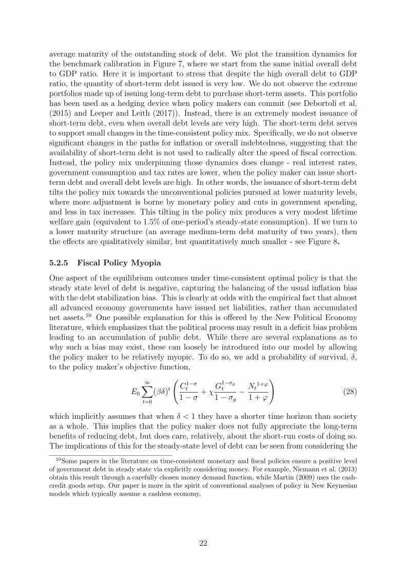
average maturity of the outstanding stock of debt. We plot the transition dynamics forthe benchmark calibration in Figure 7, where we start from the same initial overall debtto GDP ratio. Here it is important to stress that despite the high overall debt to GDPratio, the quantity of short-term debt issued is very low. We do not observe the extremeportfolios made up of issuing long-term debt to purchase short-term assets. This portfoliohas been used as a hedging device when policy makers can commit (see Debortoli et al.(2015) and Leeper and Leith (2017)). Instead, there is an extremely modest issuance ofshort-term debt, even when overall debt levels are very high. The short-term debt servesto support small changes in the time-consistent policy mix. Specifically, we do not observesignificant changes in the paths for inflation or overall indebtedness, suggesting that theavailability of short-term debt is not used to radically alter the speed of fiscal correction.Instead, the policy mix underpinning those dynamics does change - real interest rates,government consumption and tax rates are lower, when the policy maker can issue short-term debt and overall debt levels are high. In other words, the issuance of short-term debttilts the policy mix towards the unconventional policies pursued at lower maturity levels,where more adjustment is borne by monetary policy and cuts in government spending,and less in tax increases. This tilting in the policy mix produces a very modest lifetimewelfare gain (equivalent to 1.5% of one-period’s steady-state consumption). If we turn toa lower maturity structure (an average medium-term debt maturity of two years), thenthe effects are qualitatively similar, but quantitatively much smaller - see Figure 8.
5.2.5 Fiscal Policy Myopia
One aspect of the equilibrium outcomes under time-consistent optimal policy is that thesteady state level of debt is negative, capturing the balancing of the usual inflation biaswith the debt stabilization bias. This is clearly at odds with the empirical fact that almostall advanced economy governments have issued net liabilities, rather than accumulatednet assets.10 One possible explanation for this is offered by the New Political Economyliterature, which emphasizes that the political process may result in a deficit bias problemleading to an accumulation of public debt. While there are several explanations as towhy such a bias may exist, these can loosely be introduced into our model by allowingthe policy maker to be relatively myopic. To do so, we add a probability of survival, δ,to the policy maker’s objective function,
E0
∞∑t=0
(βδ)t
(C1−σt
1− σ+ χ
G1−σgt
1− σg− Nt
1+ϕ
1 + ϕ
)(28)
which implicitly assumes that when δ < 1 they have a shorter time horizon than societyas a whole. This implies that the policy maker does not fully appreciate the long-termbenefits of reducing debt, but does care, relatively, about the short-run costs of doing so.The implications of this for the steady-state level of debt can be seen from considering the
10Some papers in the literature on time-consistent monetary and fiscal policies ensure a positive levelof government debt in steady state via explicitly considering money. For example, Niemann et al. (2013)obtain this result through a carefully chosen money demand function, while Martin (2009) uses the cash-credit goods setup. Our paper is more in the spirit of conventional analyses of policy in New Keynesianmodels which typically assume a cashless economy.
22
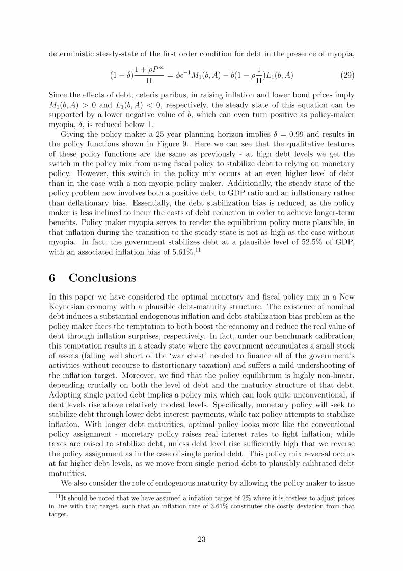
deterministic steady-state of the first order condition for debt in the presence of myopia,
(1− δ)1 + ρPm
Π= φε−1M1(b, A)− b(1− ρ 1
Π)L1(b, A) (29)
Since the effects of debt, ceteris paribus, in raising inflation and lower bond prices implyM1(b, A) > 0 and L1(b, A) < 0, respectively, the steady state of this equation can besupported by a lower negative value of b, which can even turn positive as policy-makermyopia, δ, is reduced below 1.
Giving the policy maker a 25 year planning horizon implies δ = 0.99 and results inthe policy functions shown in Figure 9. Here we can see that the qualitative featuresof these policy functions are the same as previously - at high debt levels we get theswitch in the policy mix from using fiscal policy to stabilize debt to relying on monetarypolicy. However, this switch in the policy mix occurs at an even higher level of debtthan in the case with a non-myopic policy maker. Additionally, the steady state of thepolicy problem now involves both a positive debt to GDP ratio and an inflationary ratherthan deflationary bias. Essentially, the debt stabilization bias is reduced, as the policymaker is less inclined to incur the costs of debt reduction in order to achieve longer-termbenefits. Policy maker myopia serves to render the equilibrium policy more plausible, inthat inflation during the transition to the steady state is not as high as the case withoutmyopia. In fact, the government stabilizes debt at a plausible level of 52.5% of GDP,with an associated inflation bias of 5.61%.11
6 Conclusions
In this paper we have considered the optimal monetary and fiscal policy mix in a NewKeynesian economy with a plausible debt-maturity structure. The existence of nominaldebt induces a substantial endogenous inflation and debt stabilization bias problem as thepolicy maker faces the temptation to both boost the economy and reduce the real value ofdebt through inflation surprises, respectively. In fact, under our benchmark calibration,this temptation results in a steady state where the government accumulates a small stockof assets (falling well short of the ‘war chest’ needed to finance all of the government’sactivities without recourse to distortionary taxation) and suffers a mild undershooting ofthe inflation target. Moreover, we find that the policy equilibrium is highly non-linear,depending crucially on both the level of debt and the maturity structure of that debt.Adopting single period debt implies a policy mix which can look quite unconventional, ifdebt levels rise above relatively modest levels. Specifically, monetary policy will seek tostabilize debt through lower debt interest payments, while tax policy attempts to stabilizeinflation. With longer debt maturities, optimal policy looks more like the conventionalpolicy assignment - monetary policy raises real interest rates to fight inflation, whiletaxes are raised to stabilize debt, unless debt level rise sufficiently high that we reversethe policy assignment as in the case of single period debt. This policy mix reversal occursat far higher debt levels, as we move from single period debt to plausibly calibrated debtmaturities.
We also consider the role of endogenous maturity by allowing the policy maker to issue
11It should be noted that we have assumed a inflation target of 2% where it is costless to adjust pricesin line with that target, such that an inflation rate of 3.61% constitutes the costly deviation from thattarget.
23

both single-period and medium maturity debt. We find that this does little to affect theunderlying inflation and debt stabilization bias problems and debt dynamics, but that amodest issuance of short-term debt allows the policy maker to shift the policy mix to bemore like that of the single period debt case with lower real interest rates, governmentconsumption and tax rates. This is mildly welfare improving. It is also interesting to notethat the implicit government debt portfolio does not attempt to achieve any of the hedgingeffects associated with some optimal policy exercises when the policy maker can commit.Finally, we allow the policy maker to be relatively myopic in evaluating the future ina manner which mimics the various explanations of the deficit bias problem. We findthat this does not qualitatively affect the debt-dependent bifurcation in the policy mixdetailed in the paper, although it does for even a relatively modest degree of myopia turnthe steady-state debt level positive and support an inflationary rather than deflationarybias, bringing us closer to understanding empirically observed debt dynamics.
24

References
Aiyagari, S. R., A. Marcet, T. J. Sargent, and J. Seppala (2002). Optimal Taxationwithout State-Contingent Debt. Journal of Political Economy 110 (6), 1220–1254.
Alesina, A. and A. Passalacqua (2017). The political economy of government debt. Forth-coming in Taylor, J. and H. Uhlig (eds), the Handbook of Macroeconomics, Volume 2 .
Anderson, G. S., J. Kim, and T. Yun (2010). Using a projection method to analyze infla-tion bias in a micro-founded model. Journal of Economic Dynamics and Control 34 (9),1572–1581.
Angeletos, G.-M., F. Collard, H. Dellas, and B. Diba (2013). Optimal public debt man-agement and liquidity provision. NBER Working Paper 18800 .
Barro, R. J. (1979). On the determination of the public debt. The Journal of PoliticalEconomy , 940–971.
Benigno, P. and M. Woodford (2003). Optimal monetary and fiscal policy: A linear-quadratic approach. In NBER Macroeconomics Annual 2003, Volume 18, pp. 271–364.The MIT Press.
Bhattarai, S., G. B. Eggertsson, and B. Gafarov (2014). Time Consistency and theDuration of Government Debt: A Signalling Theory of Quantitative Easing. Mimeo.
Bi, H., E. M. Leeper, and C. Leith (2013). Uncertain fiscal consolidations. The EconomicJournal 123 (566), F31–F63.
Calmfors, L. and S. Wren-Lewis (2011). What should fiscal councils do? EconomicPolicy 26 (68), 649–695.
Cao, Q. (2014). Optimal Fiscal and Monetary Policy with Collateral Constraints. Mimeo.
Corhay, A., H. Kung, and G. Morales (2014). Government maturity structure twists.Mimeo.
Debortoli, D. and R. Nunes (2013). Lack of Commitment and the Level of Debt. Journalof the European Economic Association 11 (5), 1053–1078.
Debortoli, D., R. Nunes, and P. Yared (2015). Optimal Time-Consistent GovernmentDebt Maturity. Mimeo.
Eusepi, S. and B. Preston (2011). The maturity structure of debt, monetary policy andexpectations stabilization. mimeo, Columbia University .
Eusepi, S. and B. J. Preston (2013). Fiscal Foundations of Inflation: Imperfect Knowl-edge. FRB of New York Staff Report No. 649 (649).
Faraglia, E., A. Marcet, R. Oikonomou, and A. Scott (2013). The impact of debt levelsand debt maturity on inflation. The Economic Journal 123 (566), F164–F192.
Faraglia, E., A. Marcet, and A. Scott (2014). Modelling Long Bonds-The Case of OptimalFiscal Policy. Mimeo.
25

Grechyna, D. (2013). Debt and Deficit Fluctuations in a Time-Consistent Setup. Availableat SSRN 1997563 .
Greenwood, R., S. G. Hanson, J. S. Rudolph, and L. H. Summers (2014). GovernmentDebt Management at the Zero Lower Bound. Mimeo.
Hall, G. J. and T. J. Sargent (2011). Interest Rate Risk and Other Determinants of Post-WWII US Government Debt/GDP Dynamics. American Economic Journal: Macroe-conomics 3 (3), 192–214.
International Monetary Fund (2012). Balancing Fiscal Risks. Fiscal Monitor April 2011.
Judd, K. L. (1998). Numerical Methods in Economics. MIT press.
Judd, K. L. (2004). Existence, uniqueness, and computational theory for time consistentequilibria: A hyperbolic discounting example. mimeo, Stanford University .
Klein, P., P. Krusell, and J.-V. Rios-Rull (2008). Time-consistent public policy. TheReview of Economic Studies 75 (3), 789–808.
Klein, P. and J.-V. Rios-Rull (2003). Time-consistent optimal fiscal policy*. InternationalEconomic Review 44 (4), 1217–1245.
Krusell, P., F. Martin, and J.-V. Rıos-Rull (2006). Time-consistent debt. Mimeo.
Lagos, R. and R. Wright (2005). A Unified Framework for Monetary Theory and PolicyAnalysis. Journal of Political Economy 113 (3), pp. 463–484.
Leeper, E. and C. Leith (2017). Understanding inflation as a joint monetary-fiscal phe-nomenon. Forthcoming in Taylor, J. and H. Uhlig (eds), the Handbook of Macroeco-nomics, Volume 2 .
Leeper, E. M. and X. Zhou (2013). Inflation’s Role in Optimal Monetary-Fiscal Policy.NBER Working Paper No. 19686 .
Leith, C. and D. Liu (2014). The Inflation Bias Under Calvo and Rotemberg Pricing.University of Glasgow Discussion Paper No. 2014-6 .
Leith, C. and S. Wren-Lewis (2013). Fiscal Sustainability in a New Keynesian Model.Journal of Money, Credit and Banking 45 (8), 1477–1516.
Lucas, R. E. J. and N. L. Stokey (1983). Optimal fiscal and monetary policy in aneconomy without capital. Journal of monetary Economics 12 (1), 55–93.
Martin, F. M. (2009). A positive theory of government debt. Review of economic Dy-namics 12 (4), 608–631.
Martin, F. M. (2011). On the joint determination of fiscal and monetary policy. Journalof Monetary Economics 58 (2), 132–145.
Martin, F. M. (2013). Government Policy in Monetary Economies. International Eco-nomic Review 54 (1), 185–217.
26
Martin, F. M. (2014). The Value of Constraints on Discretionary Government Policy.Mimeo.
Matveev, D. (2014). Time-Consistent Management of a Liquidity Trap: Monetary andFiscal policy with Debt. Mimeo.
Nakata, T. (2013). Optimal fiscal and monetary policy with occasionally binding zerobound constraints. Federal Reserve Board Finance and Economics Discussion Series,2013-40 .
Ngo, P. V. (2014). Optimal discretionary monetary policy in a micro-founded modelwith a zero lower bound on nominal interest rate. Journal of Economic Dynamics andControl 45 (0), 44 – 65.
Niemann, S. and P. Pichler (2011). Optimal fiscal and monetary policies in the face ofrare disasters. European Economic Review 55 (1), 75–92.
Niemann, S., P. Pichler, and G. Sorger (2013). Public debt, discretionary policy, andinflation persistence. Journal of Economic Dynamics and Control 37 (6), 1097–1109.
Ortigueira, S. (2006). Markov-perfect optimal taxation. Review of Economic Dynam-ics 9 (1), 153–178.
Ortigueira, S., J. Pereira, and P. Pichler (2012). Markov-perfect optimal fiscal policy:the case of unbalanced budgets. Mimeo.
Rotemberg, J. J. (1982). Sticky Prices in the United States. Journal of Political Econ-omy 90 (6), 1187–1211.
Schmitt-Grohe, S. and M. Uribe (2004a). Optimal fiscal and monetary policy underimperfect competition. Journal of Macroeconomics 26 (2), 183–209.
Schmitt-Grohe, S. and M. Uribe (2004b). Optimal fiscal and monetary policy understicky prices. Journal of Economic Theory 114 (2), 198–230.
Sims, C. A. (2013). Paper money. The American Economic Review 103 (2), 563–584.
Siu, H. E. (2004). Optimal fiscal and monetary policy with sticky prices. Journal ofMonetary Economics 51 (3), 575–607.
Van Zandweghe, W. and A. Wolman (2011). Discretionary monetary policy in the Calvomodel. Federal Reserve Bank of Richmond Working Paper Series, WP11-03 .
Woodford, M. (2001). Fiscal Requirements for Price Stability. Journal of Money, Creditand Banking 33 (3), 669–728.
27

A Tables
Table 1: Parameterization
Parameter Value Definitionβ 0.995 Quarterly discount factorσ 2 Relative risk aversion coefficientσg 2 Relative risk aversion coefficient for government spendingϕ 3 Inverse Frish elasticity of labor supplyε 21 Elasticity of substitution between varietiesρ 0.95 Debt maturity structureχ 0.055 Scaling parameter associated with government spendingρa 0.95 AR-coefficient of technology shockσa 0.01 Standard deviation of technology shockφ 32.5 Rotemberg adjustment cost coefficientΠ∗ 2% Annual inflation rate target
28
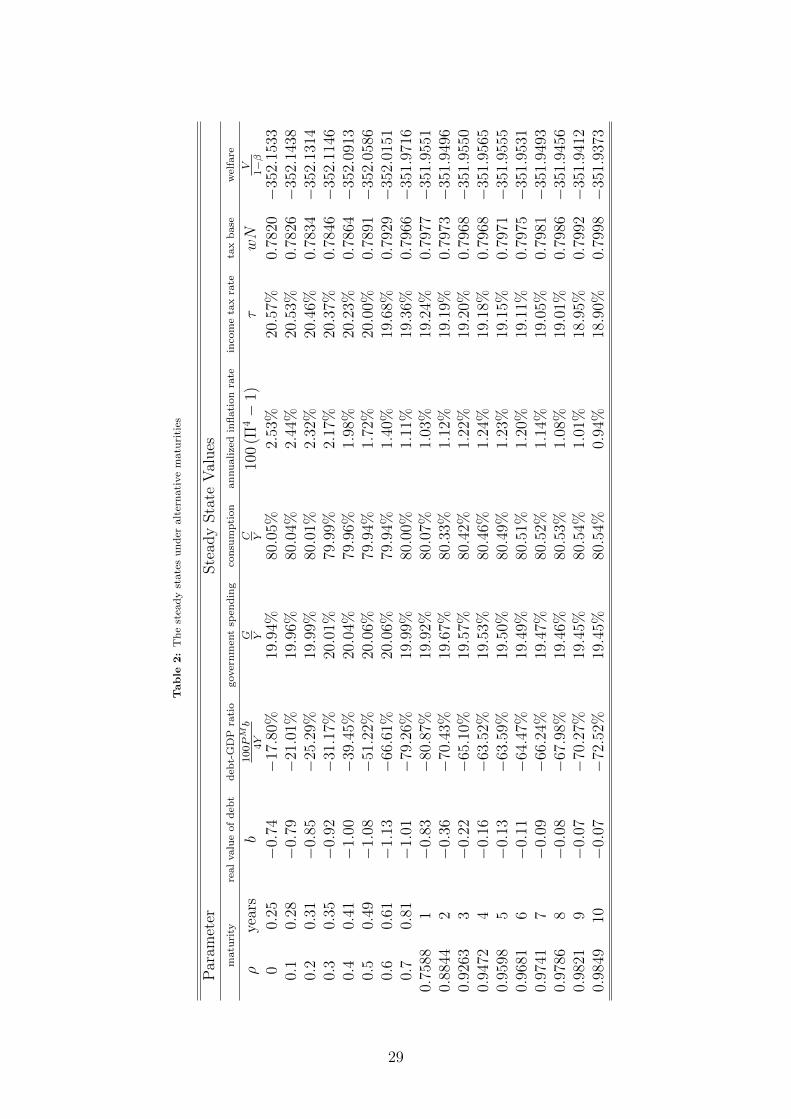
Table
2:
Th
est
ead
yst
ate
su
nd
eralt
ern
ati
ve
matu
riti
es
Par
amet
erSte
ady
Sta
teV
alues
matu
rity
real
valu
eof
deb
td
ebt-
GD
Pra
tio
gover
nm
ent
spen
din
gco
nsu
mp
tion
an
nu
alize
din
flati
on
rate
inco
me
tax
rate
tax
base
wel
fare
ρye
ars
b100PMb
4Y
G YC Y
100
(Π4−
1)τ
wN
V1−β
00.
25−
0.74
−17.8
0%19.9
4%80.0
5%2.
53%
20.5
7%0.
7820−
352.
1533
0.1
0.28
−0.
79−
21.0
1%19.9
6%80.0
4%2.
44%
20.5
3%0.
7826−
352.
1438
0.2
0.31
−0.
85−
25.2
9%19.9
9%80.0
1%2.
32%
20.4
6%0.
7834−
352.
1314
0.3
0.35
−0.
92−
31.1
7%20.0
1%79.9
9%2.
17%
20.3
7%0.
7846−
352.
1146
0.4
0.41
−1.
00−
39.4
5%20.0
4%79.9
6%1.
98%
20.2
3%0.
7864−
352.
0913
0.5
0.49
−1.
08−
51.2
2%20.0
6%79.9
4%1.
72%
20.0
0%0.
7891−
352.
0586
0.6
0.61
−1.
13−
66.6
1%20.0
6%79.9
4%1.
40%
19.6
8%0.
7929−
352.
0151
0.7
0.81
−1.
01−
79.2
6%19.9
9%80.0
0%1.
11%
19.3
6%0.
7966−
351.
9716
0.75
881
−0.
83−
80.8
7%19.9
2%80.0
7%1.
03%
19.2
4%0.
7977−
351.
9551
0.88
442
−0.
36−
70.4
3%19.6
7%80.3
3%1.
12%
19.1
9%0.
7973−
351.
9496
0.92
633
−0.
22−
65.1
0%19.5
7%80.4
2%1.
22%
19.2
0%0.
7968−
351.
9550
0.94
724
−0.
16−
63.5
2%19.5
3%80.4
6%1.
24%
19.1
8%0.
7968−
351.
9565
0.95
985
−0.
13−
63.5
9%19.5
0%80.4
9%1.
23%
19.1
5%0.
7971−
351.
9555
0.96
816
−0.
11−
64.4
7%19.4
9%80.5
1%1.
20%
19.1
1%0.
7975−
351.
9531
0.97
417
−0.
09−
66.2
4%19.4
7%80.5
2%1.
14%
19.0
5%0.
7981−
351.
9493
0.97
868
−0.
08−
67.9
8%19.4
6%80.5
3%1.
08%
19.0
1%0.
7986−
351.
9456
0.98
219
−0.
07−
70.2
7%19.4
5%80.5
4%1.
01%
18.9
5%0.
7992−
351.
9412
0.98
4910
−0.
07−
72.5
2%19.4
5%80.5
4%0.
94%
18.9
0%0.
7998−
351.
9373
29

B Figures
R e c e n t F I s c a l D e v e lo p M e n ts a n D o u t lo o k
International Monetary Fund | April 2015 7
1. Debt and Cyclically Adjusted Deficit, 2001–20 20
01
02 03
04
05
06
07
08
09
10
11
12
13
14
15
16
17
18
19
20
Debt
(per
cent
of G
DP)
CAD
(per
cent
of p
oten
tial G
DP)
Figure 1.2. Fiscal Trends in Advanced Economies
6. Fiscal Balance: 2014 Preliminary Outturns versus Original Budget Plans5
(Percent of GDP)
2005 0
6 0
7 0
8 0
9 1
0 1
1 1
2 1
3 1
4 1
5 1
6 1
7 1
8 1
9 2
0
2. Euro Area: Revisions to General Government Gross Debt1
(Index, 2007 = 100)
–10 –9 –8 –7 –6 –5 –4 –3 –2 –1 0 1Output gap (percent of potential GDP)
3. Need for Demand Support2 4. Fiscal Space3
0
2
4
6
8
10
12
Ten-
year
bon
d yi
eld4 (
last
thre
e
mon
ths
aver
age,
per
cent
)
Debt, 2014 (percent of GDP)
5. Average Annual Cyclically Adjusted Primary Balance Change (Percent of potential GDP)
0
1
2
3
4
5
6
7
8
60
70
80
90
100
110
90
100
110
120
130
140
150
Curr
ent a
ccou
nt b
alan
ce (p
erce
nt o
f GDP
)
–6
–4
–2
0
2
4
6
8
10
12
16
14
–2.0
–1.5
–1.0
–0.5
Sources: Thomson Reuters Datastream; and IMF staff estimates. Note: AEs = advanced economies; CAD = cyclically adjusted deficit; FM = Fiscal Monitor. Data labels in the figure use International Organization for Standardization (ISO) country codes. 1 Data for members of the European Union have been revised following the adoption of the new European System of National and Regional Accounts (ESA 2010). 2 The more negative the output gap, the larger the demand support needed. 3 The higher the level of debt and the higher the cost of financing, the lower the fiscal space. 4 For Cyprus: five-year government bond yield. 5 For the United States and Canada, the 2014 budget target for the general government corresponds to IMF staff estimates as reported in the April 2014 Fiscal Monitor; for all other countries, data come from countries' budget laws and budget execution documents.
AUTBEL
CYP
FIN
FRADEU
GRC
IRL ITA
LVA
LUX
MLT
NLD PRTSVK
SVN
ESPHigh debt
High borrowing costs
DEU
ITA
ESP
NLD
FRA
GRC
FIN
AUT
IRL
PRTBEL
CYP
SVK
SVNLUX
EST
LVA
MLT
Large internal imbalance
Large external imbalance
CAD (left scale)Debt (right scale)
0.0
0.5
1.0
1.5
KOR
SVN
FRA
JPN
ESP
FIN
GBR ITA AUS
PRT
USA
CAN
LUX
DEU
IRL
NLD
Current FM
Spring 2013
Spring 2011
Spring 2007
Spring 2009
0 50 100 150 200
Average 2010 –13 2014 2015 2016
–0.5
0.0
0.5
1.0
1.5
2.0
AEs USA Euro Area GBR JPN CAN
The average ratio of debt to GDP remains above 100 percent and is expected to decline only slowly, as very low inflation and slow growth complicate debt reduction efforts. The pace of fiscal consolidation has slowed to support economic activity. In the euro area, the fiscal space is lacking where demand support is needed the most.
Figure 1: The average debt-GDP ratio and the cyclically adjusted deficit as percent of potential GDP in advancedeconomies. CAD = cyclically adjusted deficit. Source: IMF Fiscal Monitor, 2015.
2000 2002 2004 2006 2008 20100
20
40
60
80
100
120
140
Deb
t to
GD
P R
atio
2000 2002 2004 2006 2008 2010
4
6
8
10
12
14
16
18
20
Ave
rage
Dur
atio
n of
Deb
t
GermanyGreeceItalyJapanPortugalSpainU.K.U.S.
Figure 1: Size and maturity composition of debt. The gure shows the evolution ofdebt-to-GDP ratios and average maturity of debt for a selected group of countries. The debt-to-GDP time series is measured as net nancial liabilities as a percentage of nominal GDP;the average maturity of debt is measured as the average term to maturity of total outstandinggovernment debt. The data source is the OECD database.
as a very stringent assumption.3
Consider a exible-price endowment economy with long-term government debt. Mone-
tary and scal policy are specied by simple rules. The monetary rule prescribes that the
short-term nominal rate responds more than proportionally to ination, while the scal rule
adjusts lump-sum taxes more than proportionally to changes in government debt. Under
rational expectations this policy framework induces a Ricardian equilibrium. Fiscal policy
has no monetary consequences. Now suppose agents have imperfect knowledge, modeled as
uncertainty about the long-term equilibrium level of ination and taxes. Interpret this as
either fundamental uncertainty about the policy regime, or imperfect credibility about policy
objectives. Following Marcet and Sargent (1989) and Evans and Honkapohja (2001), to learn
about the long-run objectives of policy, agents employ a simple linear econometric model
with an unobserved drift, estimated each period as new data become available. Estimates of
average ination and taxes are updated in response to past forecast errors. This is an intu-
itive model of expectations formation supported by empirical evidence.4 This kind of belief
3See Davig and Leeper (2006) and Bianchi (2010).4See Adam, Marcet, and Nicolini (2012), Adam, Beutel, and Marcet (2013), Eusepi and Preston (2011),
Milani (2007) and Slobodyan and Wouters (2012).
2
Figure 2: This figure shows the evolution of debt-to-GDP ratios and average maturity of debt for a selected group ofcountries. The debt-to-GDP time series is measured as net financial liabilities as a percentage of nominal GDP; the averagematurity of debt is measured as the average term to maturity of total outstanding government debt. Taken from Eusepiand Preston (2013).
30

-0.4 -0.2 0 0.2 0.4 0.6 0.8 1
bt
-0.5
0
0.5
1Real debt
Debt bt
45 degree Line
-0.4 -0.2 0 0.2 0.4 0.6 0.8 1
Yt
0.98
1
1.02
1.04
1.06Output
-0.4 -0.2 0 0.2 0.4 0.6 0.8 1
Ct
0.7
0.75
0.8
0.85Consumption
-0.4 -0.2 0 0.2 0.4 0.6 0.8 1
PM tbt
4Yt
-2
-1
0
1
2Debt-GDP ratio (%)
-0.4 -0.2 0 0.2 0.4 0.6 0.8 1
Gt
0.14
0.16
0.18
0.2
0.22Government spending
-0.4 -0.2 0 0.2 0.4 0.6 0.8 1
Πt
-20
0
20
40
60Annualized inflation rate(%)
-0.4 -0.2 0 0.2 0.4 0.6 0.8 1
τ t
0.1
0.2
0.3
0.4
0.5Labor income tax
-0.4 -0.2 0 0.2 0.4 0.6 0.8 1
PM t
5
10
15
20Bond price
-0.4 -0.2 0 0.2 0.4 0.6 0.8 1
i t
0
20
40
60Annualized nominal interest rate (%)
ρ=0.95, φ=32.5, at=0 and b
0=1.7
-0.4 -0.2 0 0.2 0.4 0.6 0.8 1
rt
0
2
4
6
8Annualized real interest rate (%)
Figure 3: Under the benchmark parameters, the policy rules as functions of lagged debt, when the grid for technology isfixed at A=1. The cross sign indicates steady state.
t
0 10 20 30 40 50 60 70 80 90 100
Πt
0
20
40
60
Annualized Inflation (%)
t
0 10 20 30 40 50 60 70 80 90 100
Yt
0.98
1
1.02
1.04
Output
t
0 10 20 30 40 50 60 70 80 90 100
Ct
0.7
0.75
0.8
0.85
Consumption
t
0 10 20 30 40 50 60 70 80 90 100
PM tbt
4Yt
-1
0
1
2
Debt-GDP ratio
t
0 10 20 30 40 50 60 70 80 90 100
Gt
0.1
0.15
0.2
0.25
Government spending
t
0 10 20 30 40 50 60 70 80 90 100
bt
-0.5
0
0.5
1
Real debt
t
0 10 20 30 40 50 60 70 80 90 100
τ t
0
0.2
0.4
0.6
Labor income tax
t
0 10 20 30 40 50 60 70 80 90 100
PM t
5
10
15
20
Bond price
t
0 10 20 30 40 50 60 70 80 90 100
i t
0
20
40
60
Annualized nominal interest rate (%)
t
0 10 20 30 40 50 60 70 80 90 100
rt
0
5
10
Annualized real interest rate (%)
Figure 4: Under the benchmark parameters, this figure plots the transition paths of policy variables when debt startsfrom levels consistent with currently observed debt-GDP ratios, and technology is fixed at A=1. The red dotted linesindicate steady states.
31

-5 -4 -3 -2 -1 0 1 2 3
Rea
l in
tere
st r
ate
r t (%
)
-2
0
2
4
6
8
10
ρ = 0 (one-period debt)ρ = 0.7588 (1-year debt)ρ = 0.9598 (5-year debt)ρ = 0.9786 (8-year debt)
-5 -4 -3 -2 -1 0 1 2 3
Infl
atio
n r
ate Π
t (%
)
-10
0
10
20
30
40
50
60
70
Debt-GDP ratioP
M
tbt
4Yt
-5 -4 -3 -2 -1 0 1 2 3
Tax
rat
e τ t
0.05
0.1
0.15
0.2
0.25
0.3
0.35
0.4
0.45
0.5
Debt-GDP ratioP
M
tbt
4Yt
-5 -4 -3 -2 -1 0 1 2 3
Go
ver
nm
ent
spen
din
g G
t
0.12
0.13
0.14
0.15
0.16
0.17
0.18
0.19
0.2
0.21
Figure 5: This figure illustrates the relationship between policy mix and the debt-GDP ratio under alternative maturities.The cross signs indicate steady states.
t
0 20 40 60 80 100 120
Πt
0
10
20Annualized Inflation (%)
t
0 20 40 60 80 100 120
Yt
0.98
1
1.02
1.04Output
t
0 20 40 60 80 100 120
Ct
0.8
0.82
0.84
0.86Consumption
t
0 20 40 60 80 100 120
PM tbt
4Yt
-50
0
50Debt-GDP ratio (%)
t
0 20 40 60 80 100 120
Gt
0.1
0.15
0.2
0.25Government spending
t
0 20 40 60 80 100 120
bt
-1
0
1
2Real long-term debt
t
0 20 40 60 80 100 120
τt
0.2
0.25
0.3Labor income tax
t
0 20 40 60 80 100 120
PM t
0
20
40Bond price
t
0 20 40 60 80 100 120
i t
4
6
8
10Annualized nominal interest rate (%)
t
0 20 40 60 80 100 120
rt
-10
-5
0
5Annualized real interest rate (%)
ρ=0.9786 (8-year debt maturity)ρ=0.9598 (5-year debt maturity)ρ=0.7588 (1-year debt maturity)ρ=0 (1-quarter debt maturity)
Figure 6: This figure plots the transition paths under different maturities, when the debt-GDP ratio starts from the samelevel.
32

t
0 20 40 60 80 100 120
Πt
2
3
4
5
6
7
8Annualized Inflation (%)
t
0 20 40 60 80 100 120
Yt
1.005
1.01
1.015
1.02
1.025
1.03
1.035Output
t
0 20 40 60 80 100 120
Ct
0.81
0.815
0.82
0.825
0.83Consumption
t
0 20 40 60 80 100 120
PM tbt+P
S tbS t
4Yt
-40
-20
0
20
40
60
80Overall debt-GDP ratio (%)
t
0 20 40 60 80 100 120G
t
0.194
0.196
0.198
0.2
0.202Government spending
t
0 20 40 60 80 100 120
PM tbt
4Yt
-40
-20
0
20
40
60
80Long-term debt-GDP ratio (%)
t
0 20 40 60 80 100 120
τt
0.2
0.22
0.24
0.26
0.28
0.3Labor income tax
t
0 20 40 60 80 100 120
PS tbS t
4Yt
0
0.2
0.4
0.6
0.8
1Short-term debt-GDP ratio (%)
t
0 20 40 60 80 100 120
rt
2
2.1
2.2
2.3
2.4
2.5Annualized real interest rate (%)
With short-term debt
Without short-term debt
Figure 7: This figure compares the transition paths under the benchmark case with and without short-term debt, whenthe debt-GDP ratio starts from the same level.
t
0 20 40 60 80 100 120
Πt
2
3
4
5
6
7
8
9Annualized Inflation (%)
t
0 20 40 60 80 100 120
Yt
1.005
1.01
1.015
1.02
1.025
1.03
1.035Output
t
0 20 40 60 80 100 120
Ct
0.81
0.815
0.82
0.825
0.83Consumption
t
0 20 40 60 80 100 120
PM tbt+P
S tbS t
4Yt
-40
-20
0
20
40
60
80Overall debt-GDP ratio (%)
t
0 20 40 60 80 100 120
Gt
0.192
0.194
0.196
0.198
0.2
0.202Government spending
t
0 20 40 60 80 100 120
PM tbt
4Yt
-40
-20
0
20
40
60
80Long-term debt-GDP ratio (%)
t
0 20 40 60 80 100 120
τt
0.2
0.22
0.24
0.26
0.28
0.3Labor income tax
t
0 20 40 60 80 100 120
PS tbS t
4Yt
0
0.1
0.2
0.3
0.4
0.5
0.6Short-term debt-GDP ratio (%)
t
0 20 40 60 80 100 120
rt
2
2.1
2.2
2.3
2.4
2.5Annualized real interest rate (%)
With short-term debt
Without short-term debt
Figure 8: This figure compares the transition paths under the case with debt maturity of two years, with and withoutshort-term debt, when the debt-GDP ratio starts from the same level.
33

-2 -1.5 -1 -0.5 0 0.5 1 1.5 2 2.5
Rea
l in
tere
st r
ate
r t (%
)
1
2
3
4
5
6
7
8
ρ = 0.95 (with myopia)ρ = 0.95 (without myopia)
-2 -1.5 -1 -0.5 0 0.5 1 1.5 2 2.5
Infl
atio
n r
ate Π
t (%
)
-10
0
10
20
30
40
50
60
Debt-GDP ratioP
M
tbt
4Yt
-2 -1.5 -1 -0.5 0 0.5 1 1.5 2 2.5
Tax
rat
e τ t
0.1
0.15
0.2
0.25
0.3
0.35
0.4
0.45
0.5
Debt-GDP ratioP
M
tbt
4Yt
-2 -1.5 -1 -0.5 0 0.5 1 1.5 2 2.5
Go
ver
nm
ent
spen
din
g G
t
0.12
0.13
0.14
0.15
0.16
0.17
0.18
0.19
0.2
0.21
Figure 9: This figure illustrates the relationship between policy mix and the debt-GDP ratio under the benchmark casewith and without myopia. The cross signs indicate steady states.
34

C Technical Appendix (Not for Publication)
C.1 Summary of Model
We now summerise the model and its steady state before turning to the time-consistentpolicy problem.
Consumption Euler equation,
βRtEt
(CtCt+1
)σ (PtPt+1
)= 1 (30)
Pricing of longer-term bonds,
βEt
(CtCt+1
)σ (PtPt+1
)(1 + ρPM
t+1
)= PM
t (31)
Labour supply,
Nϕt C
σt = (1− τt)
(Wt
Pt
)≡ (1− τt)wt
Resource constraint,
Yt
[1− φ
2
(Πt
Π∗− 1
)2]
= Ct +Gt (32)
Phillips curve,
0 = (1− ε) + εmct − φΠt
Π∗
(Πt
Π∗− 1
)(33)
+ φβEt
[(CtCt+1
)σYt+1
Yt
Πt+1
Π∗
(Πt+1
Π∗− 1
)]Government budget constraint,
PMt bt = (1 + ρPM
t )bt−1
Πt
− Wt
PtNtτt +Gt
= (1 + ρPMt )
bt−1
Πt
−(
τt1− τt
)N1+ϕt Cσ
t +Gt
= (1 + ρPMt )
bt−1
Πt
−(
τt1− τt
)(YtAt
)1+ϕ
Cσt +Gt (34)
Technology,Yt = AtNt (35)
Marginal costs,
mct = Wt/ (PtAt) = (1− τt)−1Y ϕt C
σt A−1−ϕt
35

The objective function for social welfare is given by,
E0
∞∑t=0
βt
(C1−σt
1− σ+ χ
G1−σgt
1− σg− (Yt/At)
1+ϕ
1 + ϕ
)(36)
There are two state variables, real debt bt and productivity at = ln (At).
C.1.1 The Deterministic Steady State
Given the system of non-linear equations, the corresponding steady state system can bewritten as follows:
A = 1
βR
Π= 1
β
Π
(1 + ρPM
)= PM
(1− τ)w = NϕCσ
Y
[1− φ
2
(Π
Π∗− 1
)2]
= C +G
(1− ε) + εmc+ φ (β − 1)
[Π
Π∗
(Π
Π∗− 1
)]= 0
PMb = (1 + ρPM)b
Π−(
τ
1− τ
)Y 1+ϕCσ +G
Y = N
mc = w = (1− τ)−1Y ϕCσ
Hence, when Π = Π∗,
PM =β
Π∗ − βρ
mc = w =ε− 1
ε
C
Y=
[(1− τ)
(ε− 1
ε
)]1/σ
Y −ϕ+σσ
G
Y= 1− C
Y= 1−
[(1− τ)
(ε− 1
ε
)]1/σ
Y −ϕ+σσ
PMb =β
1− β
[τ
(ε− 1
ε
)− G
Y
]Y
Note that,
Y ϕ+σ
(1− G
Y
)σ= (1− τ)
(ε− 1
ε
)(37)
which will be used to contrast with the allocation that would be chosen by a socialplanner.
36

C.2 Numerical Algorithm
Let st = (bt−1, at) denote the state vector at time t, where real stock of debt bt−1 isendogenous and technology At = exp(at) is exogenous and respectively, with the followinglaw of motion:
PMt bt = (1 + ρPM
t )bt−1
Πt
− wtNtτt +Gt
at = ρaat−1 + eat
where 0 ≤ ρa < 1 and technology innovation eat is an i.i.d. normal random variable,which has a zero mean and a finite standard deviation σa.
There are 7 endogenous variables and 3 Lagrangian multipliers. Correspondingly,there are 10 functional equations associated with the 10 varaibles
Ct,Yt,Πt,bt,τt,P
Mt ,Gt,λ1t,λ2t,λ3t
.
Let’s define a new function X : R2 → R10, in order to collect the policy functions of en-dogenous variables as follows:
X(st) =(Ct(st), Yt(st),Πt(st), bt(st), τt(st), P
Mt (st), Gt(st), λ1t(st), λ2t(st), λ3t(st)
)Given the specification of the function X, the equilibrium conditions can be written morecompactly as,
Γ (st, X(st), Et [Z (X(st+1))] , Et [Zb (X(st+1))]) = 0
where Γ : R2+10+3+3 → R10 summarizes the full set of dynamic equilibrium relationship,and
Z (X(st+1)) =
Z1 (X(st+1))Z2 (X(st+1))Z3 (X(st+1))
≡ M(bt, At+1)L(bt, At+1)
(Πt+1)−1 (1 + ρPMt+1
)λ3t+1
with
M(bt, At+1) = (Ct+1)−σ Yt+1Πt+1
Π∗
(Πt+1
Π∗− 1
)L(bt, At+1) = (Ct+1)−σ(Πt+1)−1(1 + ρPM
t+1)
and
Zb (X(st+1)) =
∂Z1(X(st+1))
∂bt∂Z2(X(st+1))
∂bt∂Z3(X(st+1))
∂bt
≡
∂M(bt,At+1)∂bt
∂L(bt,At+1)∂bt
∂[(Πt+1)−1(1+ρPMt+1)λ3t+1]∂bt
More specifically,
L1(bt, At+1) =∂[(Ct+1)−σ(Πt+1)−1(1 + ρPM
t+1)]
∂bt
= −σ(Ct+1)−σ−1(Πt+1)−1(1 + ρPMt+1)
∂Ct+1
∂bt
− (Ct+1)−σ(Πt+1)−2(1 + ρPMt+1)
∂Πt+1
∂bt+ ρ(Ct+1)−σ(Πt+1)−1∂P
Mt+1
∂bt
and
M1(bt, At+1) =∂[(Ct+1)−σ Yt+1
Πt+1
Π∗
(Πt+1
Π∗− 1)]
∂bt
37

= −σ(Ct+1)−σ−1Yt+1Πt+1
Π∗
(Πt+1
Π∗− 1
)∂Ct+1
∂bt+ (Ct+1)−σ
Πt+1
Π∗
(Πt+1
Π∗− 1
)∂Yt+1
∂bt
+ (Ct+1)−σYt+1
Π∗
(Πt+1
Π∗− 1
)∂Πt+1
∂bt+ (Ct+1)−σ
Yt+1
Π∗Πt+1
Π∗∂Πt+1
∂bt
= −σ(Ct+1)−σ−1Yt+1Πt+1
Π∗
(Πt+1
Π∗− 1
)∂Ct+1
∂bt+ (Ct+1)−σ
Πt+1
Π∗
(Πt+1
Π∗− 1
)∂Yt+1
∂bt
+ (Ct+1)−σYt+1
Π∗
(2Πt+1
Π∗− 1
)∂Πt+1
∂bt
Note we are assuming Et [Zb (X(st+1))] = ∂Et [Z (X(st+1))] /bt, which is normally validusing the Interchange of Integration and Differentiation Theorem. Then the problem isto find a vector-valued function X that Γ maps to the zero function. Projection methods,hence, can be used.
Following the notation convention in the literature, we simply use s = (b, a) to denotethe current state of the economy st = (bt−1, at), and s′ to represent next period statethat evolves according to the law of motion specified above. The Chebyshev collocationmethod with time iteration which we use to solve this nonlinear system can be describedas follows:
1. Define the collocation nodes and the space of the approximating functions:
• Choose an order of approximation (i.e., the polynomial degrees) nb and na foreach dimension of the state space s = (b, a), then there are Ns = (nb + 1) ×(na + 1) nodes in the state space. Let S = (S1, S2, ..., SNs) denote the set ofcollocation nodes.
• Compute the nb + 1 and na + 1 roots of the Chebychev polynomial of ordernb + 1 and na + 1 as
zib = cos
((2i− 1)π
2(nb + 1)
), for i = 1, 2, ..., nb + 1.
zia = cos
((2i− 1)π
2(na + 1)
), for i = 1, 2, ..., na + 1.
• Compute collocation points ai as
ai =a+ a
2+a− a
2zia =
a− a2
(zia + 1
)+ a
for i = 1, 2, ..., na + 1. Note that the number of collocation nodes is na + 1.Similarly, compute collocation points bi as
bi =b+ b
2+b− b
2zib =
b− b2
(zib + 1
)+ b
for i = 1, 2, ..., nb + 1, which map [−1, 1] into [b, b]. Note that
S = (bi, aj) | i = 1, 2, ..., nb + 1, j = 1, 2, ..., na + 1
that is, the tensor grids, with S1 = (b1, a1), S2 = (b1, a2), ..., SNs = (bnb+1, ana+1).
38

• The space of the approximating functions, denoted as Ω, is a matrix of two-dimensional Chebyshev polynomials. More specifically,
Ω (S) =
Ω (S1)Ω (S2)
.
.
.Ω (Sna+1)
.
.
.Ω (SNs )
=
=
1 T0(ξ(b1)T1(ξ (a1)) T0(ξ(b1)T2(ξ (a1)) · · · Tnb(ξ(b1)Tna (ξ (a1))
1 T0(ξ(b1)T1(ξ (a2)) T0(ξ(b1)T2(ξ (a2)) · · · Tnb(ξ(b1)Tna (ξ (a2))
.
.
....
.
.
. · · ·...
1 T0(ξ(b1)T1(ξ (ana+1)) T0(ξ(b1)T2(ξ (ana+1)) · · · T0(ξ(b1)Tna (ξ (ana+1))
.
.
....
.
.
. · · ·...
1 T0(ξ(bnb+1)T1(ξ (ana+1)) T0(ξ(bnb+1)T2(ξ (ana+1)) · · · T0(ξ(bnb+1)Tna (ξ (ana+1))
Ns×Ns
where ξ(x) = 2 (x− x) / (x− x)−1 maps the domain of x ∈ [x, x] into [−1, 1].
• Then, at each node s ∈ S, policy functions X(s) are approximated by X(s) =Ω(s)ΘX ,
whereΘX =
[θc, θy, θπ, θb, θτ , θp, θg, θλ1 , θλ2 , θλ3
]is a Ns × 10 matrix of the approximating coefficients.
2. Formulate an initial guess for the approximating coefficients, Θ0X , and specify the
stopping rule εtol, say, 10−6.
3. At each iteration j, we can get an updated ΘjX by implement the following time
iteration step:
• At each collocation node s ∈ S, compute the possible values of future policyfunctions X(s′) for k = 1, ..., q. That is,
X(s′) = Ω(s′)Θj−1X
where q is the number of Gauss-Hermite quadrature nodes. Note that
Ω(s′) = Tjb(ξ(b′))Tja (ξ(a′))
is a q × Ns matrix, with b′ = b(s; θb), a′ = ρaa + zk√
2σ2a, jb = 0, ..., nb, and
ja = 0, ..., na. The hat symbol indicates the corresponding approximate policyfunctions, so b is the approximate policy for real debt, for example. Similarly,the two auxilliary functions can be calculated as follows:
M(s′) ≈(C(s′; θc)
)−σY (s′; θy)
Π(s′; θπ)
Π∗
(Π(s′; θπ)
Π∗− 1
)
and,
L(s′) ≈(C(s′; θc)
)−σ (Π(s′; θπ)
)−1(
1 +ρPM
(s′; θp
)Π∗ − ρβ
)
39

Note that we use PMt = (Π∗ − ρβ)PM
t rather than PMt in numerical analysis,
since the former is far less sensitive to maturity structure variations.
• Now calculate the expectation terms E [Z (X(s′))] at each node s. Let ωkdenote the weights for the quadrature, then
E [M(s′)] ≈ 1√π
q∑k=1
ωk
(C(s′; θc)
)−σY (s′; θy)
Π(s′; θπ)
Π∗
(Π(s′; θπ)
Π∗− 1
)≡M (s′, q)
E [L(s′)] ≈ 1√π
q∑k=1
ωk
(C(s′; θc)
)−σ (Π(s′; θπ)
)−1(
1 +ρPM
(s′; θp
)Π∗ − ρβ
)≡ L (s′, q)
and
Et
[(1 + ρPM
t+1
Πt+1
)λ3t+1
]≈ 1√
π
q∑k=1
ωk
1 +ρPM(s′;θp)
Π∗−ρβ
Π(s′; θπ)
λ3(s′; θλ3) ≡ Λ (s′, q) .
Hence,
E [Z (X(s′))] ≈ E[Z (X(s′))
]=
M (s′, q)L (s′, q)Λ (s′, q)
• Next calculate the partial derivatives under expectation E [Zb (X(s′))].
• Note that we only need to compute ∂Ct+1/∂bt, ∂Yt+1/∂bt, ∂Πt+1/∂bt and ∂PMt+1/∂bt,
which are given as follows:
∂Ct+1
∂b≈
nb∑jb=0
na∑ja=0
2θcjbjab− b
T ′jb(ξ(b′))Tja(ξ(a
′)) ≡ Cb (s′)
∂Yt+1
∂bt≈
nb∑jb=0
na∑ja=0
2θyjbjab− b
T ′jb(ξ(b′))Tja(ξ(a
′)) ≡ Yb (s′)
∂Πt+1
∂bt≈
nb∑jb=0
na∑ja=0
2θπjbjab− b
T ′jb(ξ(b′))Tja(ξ(a
′)) ≡ Πb (s′)
∂PMt+1
∂bt≈
nb∑jb=0
na∑ja=0
2θpjbja(b− b
)(Π∗ − ρβ)
T ′jb(ξ(bi))Tja(ξ(aj)) ≡ PMb (s′)
Hence, we can approximate the two partial derivatives under expectation
∂E [M(s′)]
∂b
≈ 1√π
q∑k=1
ωk
−σ(C(s′; θc)
)−σ−1
Y (s′; θy) Π(s′;θπ)Π∗
(Π(s′;θπ)
Π∗− 1)Cb (s′)
+(C(s′; θc)
)−σΠ(s′;θπ)
Π∗
(Π(s′;θπ)
Π∗− 1)Yb (s′)
+(C(s′; θc)
)−σΠ(s′;θπ)
Π∗
(2Π(s′;θπ)
Π∗− 1)
Πb (s′)
40

≡ Mb (s′, q) ,
∂E [L(s′)]
∂b
≈ 1√π
q∑k=1
ωk
−σ(C(s′; θc)
)−σ−1 (Π(s′; θπ)
)−1
(1 +ρPM(s′;θp)
Π∗−ρβ )Cb (s′)
−(C(s′; θc)
)−σ (Π(s′; θπ)
)−2
(1 +ρPM(s′;θp)
Π∗−ρβ )Πb (s′)
+ρ(C(s′; θc)
)−σ (Π(s′; θπ)
)−1
PMb (s′)
≡ Lb (s′, q) .
That is,
E [Zb (X(s′))] ≈ E[Zb (X(s′))
]=
[Mb (s′, q)
Lb (s′, q)
]
4. At each collocation node s, solve for X(s) such that
Γ(s,X(s), E
[Z (X(s′))
], E[Zb (X(s′))
])= 0
The equation solver csolve written by Christopher A. Sims is employed to solvethe resulted system of nonlinear equations. With X(s) at hand, we can get thecorresponding coeffcient
ΘjX =
(Ω (S)T Ω (S)
)−1
Ω (S)T X(s)
5. Update the approximating coefficients, ΘjX = ηΘj
X + (1− η) Θj−1X , where 0 ≤ η ≤ 1
is some dampening parameter used for improving convergence.
6. Check the stopping rules. If∥∥Θj
X −Θj−1X
∥∥ < εtol, then stop, else update the ap-proximation coefficients and go back to step 3.
When implementing the above algorithm, we start from lower order Chebyshev poly-nomials and some reasonable initial guess. Then, we increase the order of approximationand take as starting value the solution from the previous lower order approximation. Thisinformal homotopy continuation idea ensures us to find a solution.
Remark. Given the fact that the price PMt fluctuates significantly for larger ρ, in
numerical analysis, we scale rule for PMt by (Π∗ − ρβ), that is, PM
t = (Π∗ − ρβ)PMt . In
this way, the steady state of PMt is very close to β, and PM
t does not differ hugely as wechange the maturity structure.
C.3 Optimal Policy Under Discretion With Endogenous Short-Term Debt
In this case, the government is allowed to issue new bonds of a different maturity andswap these for existing bonds, in a way which does not affect the wealth of the bondholders at the time of the swap, such that the exchange is voluntary.
41

The policy under discretion in this case can be described as a set of decision rules forCt, Yt,Πt, bt, τt, Gt, b
St which maximise,
V (bt−1, At, bSt−1) = max
C1−σt
1− σ+ χ
G1−σgt
1− σg− (Yt/At)
1+ϕ
1 + ϕ+ βEt
[V (bt, At+1, b
St )]
subject to the following constraints:
Yt
[1− φ
2
(Πt
Π∗− 1
)2]
= Ct +Gt
0 = (1− ε) + εmct − φΠt
Π∗
(Πt
Π∗− 1
)+ φβEt
[(CtCt+1
)σYt+1
Yt
Πt+1
Π∗
(Πt+1
Π∗− 1
)]
βEt
(CtCt+1
)σ (PtPt+1
)(1 + ρPM
t+1
)bt + βEt
(CtCt+1
)σ (PtPt+1
)bSt
=
(1 + ρβEt
(CtCt+1
)σ (PtPt+1
)(1 + ρPM
t+1
)) bt−1
Πt
+bSt−1
Πt
−(
τt1− τt
)(YtAt
)1+ϕ
Cσt +Gt
where bSt is the level of real short-term debt.Defining auxilliary functions,
M(bt, At+1, bSt ) = (Ct+1)−σ Yt+1
Πt+1
Π∗
(Πt+1
Π∗− 1
)L(bt, At+1, b
St ) = (Ct+1)−σ(Πt+1)−1(1 + ρPM
t+1)
K(bt, At+1, b
St
)= C−σt+1Π−1
t+1
we can rewrite the NKPC and government budget constraints as, respectively,
(1− ε) + ε(1− τt)−1Y ϕt C
σt A−1−ϕt − φΠt
Π∗
(Πt
Π∗− 1
)+ φβCσ
t Y−1t Et
[M(bt, At+1, b
St )]
= 0
0 = βbtCσt Et
[L(bt, At+1, b
St )]
+ βbSt Cσt Et
[K(bt, At+1, b
St
)]− bt−1
Πt
(1 + ρβCσ
t Et[L(bt, At+1, b
St )])
−bSt−1
Πt
+
(τt
1− τt
)(YtAt
)1+ϕ
Cσt −Gt
42

The Lagrangian for the policy problem can be written as,
L =
C1−σt
1− σ+ χ
G1−σgt
1− σg− (Yt/At)
1+ϕ
1 + ϕ+ βEt[V (bt, At+1, b
St )]
+ λ1t
[Yt
(1− φ
2
(Πt
Π∗− 1
)2)− Ct −Gt
]
+ λ2t
[(1− ε) + ε(1− τt)−1Y ϕ
t Cσt A−1−ϕt − φΠt
Π∗
(ΠtΠ∗− 1)
+φβCσt Y−1t Et
[M(bt, At+1, b
St )] ]
+ λ3t
βbtCσt Et
[L(bt, At+1, b
St )]
+ βbSt Cσt Et
[K(bt, At+1, b
St
)]− bt−1
Πt
(1 + ρβCσ
t Et[L(bt, At+1, b
St )])
− bSt−1
Πt+(
τt1−τt
)(YtAt
)1+ϕ
Cσt −Gt
We can write the first order conditions for the policy problem as follows:
Consumption,
C−σt − λ1t + λ2t
[σε(1− τt)−1Y ϕ
t Cσ−1t A−1−ϕ
t + σφβCσ−1t Y −1
t Et[M(bt, At+1, b
St )]]
+λ3t
[σβbtC
σ−1t Et
[L(bt, At+1, b
St )]
+ σβbSt Cσ−1t Et
[K(bt, At+1, b
St
)]−ρσβ bt−1
ΠtCσ−1t Et
[L(bt, At+1, b
St )]
+ σ(
τt1−τt
)(YtAt
)1+ϕ
Cσ−1t
]= 0
Government spending,χG−σgt − λ1t − λ3t = 0
Output,
−Y ϕt A
−1−ϕt + λ1t
[1− φ
2
(Πt
Π∗− 1
)2]
+λ2t
[εϕ(1− τt)−1Y ϕ−1
t Cσt A−1−ϕt − φβCσ
t Y−2t Et
[M(bt, At+1, b
St )]]
+λ3t
[(1 + ϕ)Y ϕ
t Cσt
(τt
1− τt
)A−1−ϕt
]= 0
Taxation,ελ2t + λ3tYt = 0
Inflation,
−λ1t
[Ytφ
Π∗
(Πt
Π∗− 1
)]− λ2t
[φ
Π∗
(2Πt
Π∗− 1
)]+λ3t
[bt−1
Π2t
(1 + ρβCσ
t Et[L(bt, At+1, b
St )])
+bSt−1
Π2t
]= 0
Government debt, bt,
βEt[V1(bt, At+1, bSt )] + λ2t
[φβCσ
t Y−1t Et
[M1(bt, At+1, b
St )]]
+βCσt λ3t
[Et[L(bt, At+1, b
St )]
+ btEt[L1(bt, At+1, b
St )]
+ bSt Et[K1
(bt, At+1, b
St
)]−ρ bt−1
ΠtEt[L1(bt, At+1, b
St )] ]
= 0
43

whereV1(bt, At+1, b
St ) ≡ ∂V (bt, At+1, b
St )/∂bt
L1(bt, At+1, bSt ) ≡ ∂L(bt, At+1, b
St )/∂bt
M1(bt, At+1, bSt ) ≡ ∂M(bt, At+1, b
St )/∂bt
K1(bt, At+1, bSt ) ≡ ∂K(bt, At+1, b
St )/∂bt
Short-term government debt, bSt ,
βEt[V3(bt, At+1, bSt )] + λ2t
[φβCσ
t Y−1t Et
[M3(bt, At+1, b
St )]]
+βCσt λ3t
[btEt
[L3(bt, At+1, b
St )]
+ Et[K(bt, At+1, b
St
)]+ bSt Et
[K3
(bt, At+1, b
St
)]−ρ bt−1
ΠtEt[L3(bt, At+1, b
St )] ]
= 0
whereV3(bt, At+1, b
St ) ≡ ∂V (bt, At+1, b
St )/∂bSt
L3(bt, At+1, bSt ) ≡ ∂L(bt, At+1, b
St )/∂bSt
M3(bt, At+1, bSt ) ≡ ∂M(bt, At+1, b
St )/∂bSt
K3(bt, At+1, bSt ) ≡ ∂K(bt, At+1, b
St )/∂bSt
Note that by the envelope theorem,
V1(bt−1, At, bSt−1) = −λ3t
Πt
(1 + ρβCσ
t Et[L(bt, At+1, b
St )])
= −λ3t
Πt
(1 + ρPM
t
)V3(bt−1, At, b
St ) = −λ3t
Πt
hence,
V1(bt, At+1, bSt ) =
λ3t+1
Πt+1
(1 + ρPM
t+1
)V3(bt, At+1, b
St ) = −λ3t+1
Πt+1
and the FOCs for government debt bt and bSt can be rewritten as, respectively,
−βEt[λ3t+1
Πt+1
(1 + ρPMt+1)
]+ λ2tφβC
σt Y−1t Et
[M1(bt, At+1, b
St )]
+βCσt λ3t
[Et[L(bt, At+1, b
St )]
+ btEt[L1(bt, At+1, b
St )]
+ bSt Et[K1
(bt, At+1, b
St
)]−ρ bt−1
ΠtEt[L1(bt, At+1, b
St )] ]
= 0
and
−βEt[λ3t+1
Πt+1
] + λ2tφβCσt Y−1t Et
[M3(bt, At+1, b
St )]
44

+βCσt λ3t
[btEt
[L3(bt, At+1, b
St )]
+ Et[K(bt, At+1, b
St
)]+ bSt Et
[K3
(bt, At+1, b
St
)]−ρ bt−1
ΠtEt[L3(bt, At+1, b
St )] ]
= 0
45


