
Package ‘qtl’February 19, 2018
Version 1.42-8
Date 2018-02-19
Title Tools for Analyzing QTL Experiments
Author Karl W Broman <[email protected]> and Hao Wu, withideas from Gary Churchill and Saunak Sen and contributions fromDanny Arends, Robert Corty, Timothee Flutre, Ritsert Jansen, PjotrPrins, Lars Ronnegard, Rohan Shah, Laura Shannon, Quoc Tran, AaronWolen, and Brian Yandell
Maintainer Karl W Broman <[email protected]>
Description Analysis of experimental crosses to identify genes(called quantitative trait loci, QTLs) contributing to variation inquantitative traits.
Depends R (>= 2.14.0)
Imports parallel, graphics, stats, utils, grDevices
Suggests testthat
License GPL-3
URL https://rqtl.org, https://github.com/kbroman/qtl
BugReports https://github.com/kbroman/qtl/issues
Encoding UTF-8
ByteCompile true
R topics documented:A starting point . . . . . . . . . . . . . . . . . . . . . . . . . . . . . . . . . . . . . . . 6add.cim.covar . . . . . . . . . . . . . . . . . . . . . . . . . . . . . . . . . . . . . . . . 10add.threshold . . . . . . . . . . . . . . . . . . . . . . . . . . . . . . . . . . . . . . . . 12addcovarint . . . . . . . . . . . . . . . . . . . . . . . . . . . . . . . . . . . . . . . . . 13addint . . . . . . . . . . . . . . . . . . . . . . . . . . . . . . . . . . . . . . . . . . . . 15addloctocross . . . . . . . . . . . . . . . . . . . . . . . . . . . . . . . . . . . . . . . . 17addmarker . . . . . . . . . . . . . . . . . . . . . . . . . . . . . . . . . . . . . . . . . . 18addpair . . . . . . . . . . . . . . . . . . . . . . . . . . . . . . . . . . . . . . . . . . . 19
1
2 R topics documented:
addqtl . . . . . . . . . . . . . . . . . . . . . . . . . . . . . . . . . . . . . . . . . . . . 22addtoqtl . . . . . . . . . . . . . . . . . . . . . . . . . . . . . . . . . . . . . . . . . . . 24allchrsplits . . . . . . . . . . . . . . . . . . . . . . . . . . . . . . . . . . . . . . . . . . 26argmax.geno . . . . . . . . . . . . . . . . . . . . . . . . . . . . . . . . . . . . . . . . . 27arithscan . . . . . . . . . . . . . . . . . . . . . . . . . . . . . . . . . . . . . . . . . . . 29arithscanperm . . . . . . . . . . . . . . . . . . . . . . . . . . . . . . . . . . . . . . . . 30badorder . . . . . . . . . . . . . . . . . . . . . . . . . . . . . . . . . . . . . . . . . . . 31bayesint . . . . . . . . . . . . . . . . . . . . . . . . . . . . . . . . . . . . . . . . . . . 32bristle3 . . . . . . . . . . . . . . . . . . . . . . . . . . . . . . . . . . . . . . . . . . . 33bristleX . . . . . . . . . . . . . . . . . . . . . . . . . . . . . . . . . . . . . . . . . . . 34c.cross . . . . . . . . . . . . . . . . . . . . . . . . . . . . . . . . . . . . . . . . . . . . 35c.scanone . . . . . . . . . . . . . . . . . . . . . . . . . . . . . . . . . . . . . . . . . . 36c.scanoneperm . . . . . . . . . . . . . . . . . . . . . . . . . . . . . . . . . . . . . . . 37c.scantwo . . . . . . . . . . . . . . . . . . . . . . . . . . . . . . . . . . . . . . . . . . 38c.scantwoperm . . . . . . . . . . . . . . . . . . . . . . . . . . . . . . . . . . . . . . . 39calc.errorlod . . . . . . . . . . . . . . . . . . . . . . . . . . . . . . . . . . . . . . . . . 40calc.genoprob . . . . . . . . . . . . . . . . . . . . . . . . . . . . . . . . . . . . . . . . 42calc.penalties . . . . . . . . . . . . . . . . . . . . . . . . . . . . . . . . . . . . . . . . 43cbind.scanoneperm . . . . . . . . . . . . . . . . . . . . . . . . . . . . . . . . . . . . . 45cbind.scantwoperm . . . . . . . . . . . . . . . . . . . . . . . . . . . . . . . . . . . . . 46checkAlleles . . . . . . . . . . . . . . . . . . . . . . . . . . . . . . . . . . . . . . . . . 47chrlen . . . . . . . . . . . . . . . . . . . . . . . . . . . . . . . . . . . . . . . . . . . . 48chrnames . . . . . . . . . . . . . . . . . . . . . . . . . . . . . . . . . . . . . . . . . . 49cim . . . . . . . . . . . . . . . . . . . . . . . . . . . . . . . . . . . . . . . . . . . . . 49clean.cross . . . . . . . . . . . . . . . . . . . . . . . . . . . . . . . . . . . . . . . . . . 51clean.scantwo . . . . . . . . . . . . . . . . . . . . . . . . . . . . . . . . . . . . . . . . 52cleanGeno . . . . . . . . . . . . . . . . . . . . . . . . . . . . . . . . . . . . . . . . . . 53comparecrosses . . . . . . . . . . . . . . . . . . . . . . . . . . . . . . . . . . . . . . . 54comparegeno . . . . . . . . . . . . . . . . . . . . . . . . . . . . . . . . . . . . . . . . 55compareorder . . . . . . . . . . . . . . . . . . . . . . . . . . . . . . . . . . . . . . . . 56condense.scantwo . . . . . . . . . . . . . . . . . . . . . . . . . . . . . . . . . . . . . . 57convert.map . . . . . . . . . . . . . . . . . . . . . . . . . . . . . . . . . . . . . . . . . 58convert.scanone . . . . . . . . . . . . . . . . . . . . . . . . . . . . . . . . . . . . . . . 59convert.scantwo . . . . . . . . . . . . . . . . . . . . . . . . . . . . . . . . . . . . . . . 60convert2riself . . . . . . . . . . . . . . . . . . . . . . . . . . . . . . . . . . . . . . . . 61convert2risib . . . . . . . . . . . . . . . . . . . . . . . . . . . . . . . . . . . . . . . . 62convert2sa . . . . . . . . . . . . . . . . . . . . . . . . . . . . . . . . . . . . . . . . . . 63countXO . . . . . . . . . . . . . . . . . . . . . . . . . . . . . . . . . . . . . . . . . . . 64drop.dupmarkers . . . . . . . . . . . . . . . . . . . . . . . . . . . . . . . . . . . . . . 65drop.markers . . . . . . . . . . . . . . . . . . . . . . . . . . . . . . . . . . . . . . . . 66drop.nullmarkers . . . . . . . . . . . . . . . . . . . . . . . . . . . . . . . . . . . . . . 66dropfromqtl . . . . . . . . . . . . . . . . . . . . . . . . . . . . . . . . . . . . . . . . . 67droponemarker . . . . . . . . . . . . . . . . . . . . . . . . . . . . . . . . . . . . . . . 68effectplot . . . . . . . . . . . . . . . . . . . . . . . . . . . . . . . . . . . . . . . . . . 70effectscan . . . . . . . . . . . . . . . . . . . . . . . . . . . . . . . . . . . . . . . . . . 72est.map . . . . . . . . . . . . . . . . . . . . . . . . . . . . . . . . . . . . . . . . . . . 74est.rf . . . . . . . . . . . . . . . . . . . . . . . . . . . . . . . . . . . . . . . . . . . . . 77fake.4way . . . . . . . . . . . . . . . . . . . . . . . . . . . . . . . . . . . . . . . . . . 78

R topics documented: 3
fake.bc . . . . . . . . . . . . . . . . . . . . . . . . . . . . . . . . . . . . . . . . . . . . 79fake.f2 . . . . . . . . . . . . . . . . . . . . . . . . . . . . . . . . . . . . . . . . . . . . 80fill.geno . . . . . . . . . . . . . . . . . . . . . . . . . . . . . . . . . . . . . . . . . . . 81find.flanking . . . . . . . . . . . . . . . . . . . . . . . . . . . . . . . . . . . . . . . . . 82find.marker . . . . . . . . . . . . . . . . . . . . . . . . . . . . . . . . . . . . . . . . . 83find.markerindex . . . . . . . . . . . . . . . . . . . . . . . . . . . . . . . . . . . . . . 84find.markerpos . . . . . . . . . . . . . . . . . . . . . . . . . . . . . . . . . . . . . . . 85find.pheno . . . . . . . . . . . . . . . . . . . . . . . . . . . . . . . . . . . . . . . . . . 86find.pseudomarker . . . . . . . . . . . . . . . . . . . . . . . . . . . . . . . . . . . . . 86findDupMarkers . . . . . . . . . . . . . . . . . . . . . . . . . . . . . . . . . . . . . . . 87fitqtl . . . . . . . . . . . . . . . . . . . . . . . . . . . . . . . . . . . . . . . . . . . . . 89fitstahl . . . . . . . . . . . . . . . . . . . . . . . . . . . . . . . . . . . . . . . . . . . . 92flip.order . . . . . . . . . . . . . . . . . . . . . . . . . . . . . . . . . . . . . . . . . . . 94formLinkageGroups . . . . . . . . . . . . . . . . . . . . . . . . . . . . . . . . . . . . . 95formMarkerCovar . . . . . . . . . . . . . . . . . . . . . . . . . . . . . . . . . . . . . . 96geno.crosstab . . . . . . . . . . . . . . . . . . . . . . . . . . . . . . . . . . . . . . . . 97geno.image . . . . . . . . . . . . . . . . . . . . . . . . . . . . . . . . . . . . . . . . . 98geno.table . . . . . . . . . . . . . . . . . . . . . . . . . . . . . . . . . . . . . . . . . . 99getid . . . . . . . . . . . . . . . . . . . . . . . . . . . . . . . . . . . . . . . . . . . . . 100groupclusteredheatmap . . . . . . . . . . . . . . . . . . . . . . . . . . . . . . . . . . . 101hyper . . . . . . . . . . . . . . . . . . . . . . . . . . . . . . . . . . . . . . . . . . . . 102inferFounderHap . . . . . . . . . . . . . . . . . . . . . . . . . . . . . . . . . . . . . . 103inferredpartitions . . . . . . . . . . . . . . . . . . . . . . . . . . . . . . . . . . . . . . 104interpPositions . . . . . . . . . . . . . . . . . . . . . . . . . . . . . . . . . . . . . . . 106jittermap . . . . . . . . . . . . . . . . . . . . . . . . . . . . . . . . . . . . . . . . . . . 107listeria . . . . . . . . . . . . . . . . . . . . . . . . . . . . . . . . . . . . . . . . . . . . 108locateXO . . . . . . . . . . . . . . . . . . . . . . . . . . . . . . . . . . . . . . . . . . 109locations . . . . . . . . . . . . . . . . . . . . . . . . . . . . . . . . . . . . . . . . . . . 110lodint . . . . . . . . . . . . . . . . . . . . . . . . . . . . . . . . . . . . . . . . . . . . 111makeqtl . . . . . . . . . . . . . . . . . . . . . . . . . . . . . . . . . . . . . . . . . . . 112map10 . . . . . . . . . . . . . . . . . . . . . . . . . . . . . . . . . . . . . . . . . . . . 114map2table . . . . . . . . . . . . . . . . . . . . . . . . . . . . . . . . . . . . . . . . . . 115mapthis . . . . . . . . . . . . . . . . . . . . . . . . . . . . . . . . . . . . . . . . . . . 116markerlrt . . . . . . . . . . . . . . . . . . . . . . . . . . . . . . . . . . . . . . . . . . 117markernames . . . . . . . . . . . . . . . . . . . . . . . . . . . . . . . . . . . . . . . . 117max.scanone . . . . . . . . . . . . . . . . . . . . . . . . . . . . . . . . . . . . . . . . . 118max.scanPhyloQTL . . . . . . . . . . . . . . . . . . . . . . . . . . . . . . . . . . . . . 119max.scantwo . . . . . . . . . . . . . . . . . . . . . . . . . . . . . . . . . . . . . . . . 121movemarker . . . . . . . . . . . . . . . . . . . . . . . . . . . . . . . . . . . . . . . . . 123MQM . . . . . . . . . . . . . . . . . . . . . . . . . . . . . . . . . . . . . . . . . . . . 124mqmaugment . . . . . . . . . . . . . . . . . . . . . . . . . . . . . . . . . . . . . . . . 126mqmautocofactors . . . . . . . . . . . . . . . . . . . . . . . . . . . . . . . . . . . . . . 128mqmextractmarkers . . . . . . . . . . . . . . . . . . . . . . . . . . . . . . . . . . . . . 129mqmfind.marker . . . . . . . . . . . . . . . . . . . . . . . . . . . . . . . . . . . . . . . 130mqmgetmodel . . . . . . . . . . . . . . . . . . . . . . . . . . . . . . . . . . . . . . . . 131mqmpermutation . . . . . . . . . . . . . . . . . . . . . . . . . . . . . . . . . . . . . . 133mqmplot.circle . . . . . . . . . . . . . . . . . . . . . . . . . . . . . . . . . . . . . . . 135mqmplot.cistrans . . . . . . . . . . . . . . . . . . . . . . . . . . . . . . . . . . . . . . 137
4 R topics documented:
mqmplot.clusteredheatmap . . . . . . . . . . . . . . . . . . . . . . . . . . . . . . . . . 138mqmplot.cofactors . . . . . . . . . . . . . . . . . . . . . . . . . . . . . . . . . . . . . 139mqmplot.directedqtl . . . . . . . . . . . . . . . . . . . . . . . . . . . . . . . . . . . . . 140mqmplot.heatmap . . . . . . . . . . . . . . . . . . . . . . . . . . . . . . . . . . . . . . 142mqmplot.multitrait . . . . . . . . . . . . . . . . . . . . . . . . . . . . . . . . . . . . . 143mqmplot.permutations . . . . . . . . . . . . . . . . . . . . . . . . . . . . . . . . . . . 144mqmplot.singletrait . . . . . . . . . . . . . . . . . . . . . . . . . . . . . . . . . . . . . 145mqmprocesspermutation . . . . . . . . . . . . . . . . . . . . . . . . . . . . . . . . . . 146mqmscan . . . . . . . . . . . . . . . . . . . . . . . . . . . . . . . . . . . . . . . . . . 148mqmscanall . . . . . . . . . . . . . . . . . . . . . . . . . . . . . . . . . . . . . . . . . 150mqmscanfdr . . . . . . . . . . . . . . . . . . . . . . . . . . . . . . . . . . . . . . . . . 152mqmsetcofactors . . . . . . . . . . . . . . . . . . . . . . . . . . . . . . . . . . . . . . 154mqmtestnormal . . . . . . . . . . . . . . . . . . . . . . . . . . . . . . . . . . . . . . . 155multitrait . . . . . . . . . . . . . . . . . . . . . . . . . . . . . . . . . . . . . . . . . . 156nchr . . . . . . . . . . . . . . . . . . . . . . . . . . . . . . . . . . . . . . . . . . . . . 157nind . . . . . . . . . . . . . . . . . . . . . . . . . . . . . . . . . . . . . . . . . . . . . 158nmar . . . . . . . . . . . . . . . . . . . . . . . . . . . . . . . . . . . . . . . . . . . . . 159nmissing . . . . . . . . . . . . . . . . . . . . . . . . . . . . . . . . . . . . . . . . . . . 159nphe . . . . . . . . . . . . . . . . . . . . . . . . . . . . . . . . . . . . . . . . . . . . . 160nqrank . . . . . . . . . . . . . . . . . . . . . . . . . . . . . . . . . . . . . . . . . . . . 161nqtl . . . . . . . . . . . . . . . . . . . . . . . . . . . . . . . . . . . . . . . . . . . . . 162ntyped . . . . . . . . . . . . . . . . . . . . . . . . . . . . . . . . . . . . . . . . . . . . 163nullmarkers . . . . . . . . . . . . . . . . . . . . . . . . . . . . . . . . . . . . . . . . . 164orderMarkers . . . . . . . . . . . . . . . . . . . . . . . . . . . . . . . . . . . . . . . . 165phenames . . . . . . . . . . . . . . . . . . . . . . . . . . . . . . . . . . . . . . . . . . 166pickMarkerSubset . . . . . . . . . . . . . . . . . . . . . . . . . . . . . . . . . . . . . . 167plot.cross . . . . . . . . . . . . . . . . . . . . . . . . . . . . . . . . . . . . . . . . . . 168plot.qtl . . . . . . . . . . . . . . . . . . . . . . . . . . . . . . . . . . . . . . . . . . . . 169plot.rfmatrix . . . . . . . . . . . . . . . . . . . . . . . . . . . . . . . . . . . . . . . . . 171plot.scanone . . . . . . . . . . . . . . . . . . . . . . . . . . . . . . . . . . . . . . . . . 172plot.scanoneboot . . . . . . . . . . . . . . . . . . . . . . . . . . . . . . . . . . . . . . 174plot.scanoneperm . . . . . . . . . . . . . . . . . . . . . . . . . . . . . . . . . . . . . . 175plot.scanPhyloQTL . . . . . . . . . . . . . . . . . . . . . . . . . . . . . . . . . . . . . 176plot.scantwo . . . . . . . . . . . . . . . . . . . . . . . . . . . . . . . . . . . . . . . . . 178plot.scantwoperm . . . . . . . . . . . . . . . . . . . . . . . . . . . . . . . . . . . . . . 180plotErrorlod . . . . . . . . . . . . . . . . . . . . . . . . . . . . . . . . . . . . . . . . . 181plotGeno . . . . . . . . . . . . . . . . . . . . . . . . . . . . . . . . . . . . . . . . . . 183plotInfo . . . . . . . . . . . . . . . . . . . . . . . . . . . . . . . . . . . . . . . . . . . 184plotLodProfile . . . . . . . . . . . . . . . . . . . . . . . . . . . . . . . . . . . . . . . . 186plotMap . . . . . . . . . . . . . . . . . . . . . . . . . . . . . . . . . . . . . . . . . . . 188plotMissing . . . . . . . . . . . . . . . . . . . . . . . . . . . . . . . . . . . . . . . . . 190plotModel . . . . . . . . . . . . . . . . . . . . . . . . . . . . . . . . . . . . . . . . . . 191plotPheno . . . . . . . . . . . . . . . . . . . . . . . . . . . . . . . . . . . . . . . . . . 193plotPXG . . . . . . . . . . . . . . . . . . . . . . . . . . . . . . . . . . . . . . . . . . . 194plotRF . . . . . . . . . . . . . . . . . . . . . . . . . . . . . . . . . . . . . . . . . . . . 195pull.argmaxgeno . . . . . . . . . . . . . . . . . . . . . . . . . . . . . . . . . . . . . . 197pull.draws . . . . . . . . . . . . . . . . . . . . . . . . . . . . . . . . . . . . . . . . . . 198pull.geno . . . . . . . . . . . . . . . . . . . . . . . . . . . . . . . . . . . . . . . . . . 199
R topics documented: 5
pull.genoprob . . . . . . . . . . . . . . . . . . . . . . . . . . . . . . . . . . . . . . . . 200pull.map . . . . . . . . . . . . . . . . . . . . . . . . . . . . . . . . . . . . . . . . . . . 201pull.markers . . . . . . . . . . . . . . . . . . . . . . . . . . . . . . . . . . . . . . . . . 202pull.pheno . . . . . . . . . . . . . . . . . . . . . . . . . . . . . . . . . . . . . . . . . . 202pull.rf . . . . . . . . . . . . . . . . . . . . . . . . . . . . . . . . . . . . . . . . . . . . 203qtlversion . . . . . . . . . . . . . . . . . . . . . . . . . . . . . . . . . . . . . . . . . . 204read.cross . . . . . . . . . . . . . . . . . . . . . . . . . . . . . . . . . . . . . . . . . . 205readMWril . . . . . . . . . . . . . . . . . . . . . . . . . . . . . . . . . . . . . . . . . . 212reduce2grid . . . . . . . . . . . . . . . . . . . . . . . . . . . . . . . . . . . . . . . . . 213refineqtl . . . . . . . . . . . . . . . . . . . . . . . . . . . . . . . . . . . . . . . . . . . 214reorderqtl . . . . . . . . . . . . . . . . . . . . . . . . . . . . . . . . . . . . . . . . . . 216replace.map . . . . . . . . . . . . . . . . . . . . . . . . . . . . . . . . . . . . . . . . . 217replacemap.scanone . . . . . . . . . . . . . . . . . . . . . . . . . . . . . . . . . . . . . 218replacemap.scantwo . . . . . . . . . . . . . . . . . . . . . . . . . . . . . . . . . . . . . 219replaceqtl . . . . . . . . . . . . . . . . . . . . . . . . . . . . . . . . . . . . . . . . . . 220rescalemap . . . . . . . . . . . . . . . . . . . . . . . . . . . . . . . . . . . . . . . . . 221ripple . . . . . . . . . . . . . . . . . . . . . . . . . . . . . . . . . . . . . . . . . . . . 222scanone . . . . . . . . . . . . . . . . . . . . . . . . . . . . . . . . . . . . . . . . . . . 224scanoneboot . . . . . . . . . . . . . . . . . . . . . . . . . . . . . . . . . . . . . . . . . 232scanonevar . . . . . . . . . . . . . . . . . . . . . . . . . . . . . . . . . . . . . . . . . . 234scanonevar.meanperm . . . . . . . . . . . . . . . . . . . . . . . . . . . . . . . . . . . . 236scanonevar.varperm . . . . . . . . . . . . . . . . . . . . . . . . . . . . . . . . . . . . . 237scanPhyloQTL . . . . . . . . . . . . . . . . . . . . . . . . . . . . . . . . . . . . . . . 238scanqtl . . . . . . . . . . . . . . . . . . . . . . . . . . . . . . . . . . . . . . . . . . . . 240scantwo . . . . . . . . . . . . . . . . . . . . . . . . . . . . . . . . . . . . . . . . . . . 242scantwopermhk . . . . . . . . . . . . . . . . . . . . . . . . . . . . . . . . . . . . . . . 247shiftmap . . . . . . . . . . . . . . . . . . . . . . . . . . . . . . . . . . . . . . . . . . . 249sim.cross . . . . . . . . . . . . . . . . . . . . . . . . . . . . . . . . . . . . . . . . . . 250sim.geno . . . . . . . . . . . . . . . . . . . . . . . . . . . . . . . . . . . . . . . . . . . 253sim.map . . . . . . . . . . . . . . . . . . . . . . . . . . . . . . . . . . . . . . . . . . . 254simFounderSnps . . . . . . . . . . . . . . . . . . . . . . . . . . . . . . . . . . . . . . 256simPhyloQTL . . . . . . . . . . . . . . . . . . . . . . . . . . . . . . . . . . . . . . . . 257simulatemissingdata . . . . . . . . . . . . . . . . . . . . . . . . . . . . . . . . . . . . . 259stepwiseqtl . . . . . . . . . . . . . . . . . . . . . . . . . . . . . . . . . . . . . . . . . 260strip.partials . . . . . . . . . . . . . . . . . . . . . . . . . . . . . . . . . . . . . . . . . 264subset.cross . . . . . . . . . . . . . . . . . . . . . . . . . . . . . . . . . . . . . . . . . 265subset.map . . . . . . . . . . . . . . . . . . . . . . . . . . . . . . . . . . . . . . . . . 267subset.scanone . . . . . . . . . . . . . . . . . . . . . . . . . . . . . . . . . . . . . . . 268subset.scanoneperm . . . . . . . . . . . . . . . . . . . . . . . . . . . . . . . . . . . . . 269subset.scantwo . . . . . . . . . . . . . . . . . . . . . . . . . . . . . . . . . . . . . . . 270subset.scantwoperm . . . . . . . . . . . . . . . . . . . . . . . . . . . . . . . . . . . . . 271summary.cross . . . . . . . . . . . . . . . . . . . . . . . . . . . . . . . . . . . . . . . 272summary.fitqtl . . . . . . . . . . . . . . . . . . . . . . . . . . . . . . . . . . . . . . . . 272summary.qtl . . . . . . . . . . . . . . . . . . . . . . . . . . . . . . . . . . . . . . . . . 273summary.ripple . . . . . . . . . . . . . . . . . . . . . . . . . . . . . . . . . . . . . . . 274summary.scanone . . . . . . . . . . . . . . . . . . . . . . . . . . . . . . . . . . . . . . 275summary.scanoneboot . . . . . . . . . . . . . . . . . . . . . . . . . . . . . . . . . . . . 279summary.scanoneperm . . . . . . . . . . . . . . . . . . . . . . . . . . . . . . . . . . . 280

6 A starting point
summary.scanPhyloQTL . . . . . . . . . . . . . . . . . . . . . . . . . . . . . . . . . . 281summary.scantwo . . . . . . . . . . . . . . . . . . . . . . . . . . . . . . . . . . . . . . 283summary.scantwoperm . . . . . . . . . . . . . . . . . . . . . . . . . . . . . . . . . . . 286summaryMap . . . . . . . . . . . . . . . . . . . . . . . . . . . . . . . . . . . . . . . . 288summaryScantwoOld . . . . . . . . . . . . . . . . . . . . . . . . . . . . . . . . . . . . 289switch.order . . . . . . . . . . . . . . . . . . . . . . . . . . . . . . . . . . . . . . . . . 290switchAlleles . . . . . . . . . . . . . . . . . . . . . . . . . . . . . . . . . . . . . . . . 291table2map . . . . . . . . . . . . . . . . . . . . . . . . . . . . . . . . . . . . . . . . . . 292top.errorlod . . . . . . . . . . . . . . . . . . . . . . . . . . . . . . . . . . . . . . . . . 293totmar . . . . . . . . . . . . . . . . . . . . . . . . . . . . . . . . . . . . . . . . . . . . 294transformPheno . . . . . . . . . . . . . . . . . . . . . . . . . . . . . . . . . . . . . . . 295tryallpositions . . . . . . . . . . . . . . . . . . . . . . . . . . . . . . . . . . . . . . . . 296typingGap . . . . . . . . . . . . . . . . . . . . . . . . . . . . . . . . . . . . . . . . . . 297write.cross . . . . . . . . . . . . . . . . . . . . . . . . . . . . . . . . . . . . . . . . . . 299xaxisloc.scanone . . . . . . . . . . . . . . . . . . . . . . . . . . . . . . . . . . . . . . 301
Index 303
A starting point Introductory comments on R/qtl
Description
A brief introduction to the R/qtl package, with a walk-through of an analysis.
New to R and/or R/qtl?
• In order to use the R/qtl package, you must type (within R) library(qtl). You may wish toinclude this in a .Rprofile file.
• Documention and several tutorials are available at the R archive (https://cran.r-project.org).
• Use the help.start function to start the html version of the R help.
• Type library(help=qtl) to get a list of the functions in R/qtl.
• Use the example function to run examples of the various functions in R/qtl.
• A tutorial on the use of R/qtl is distributed with the package and is also available at https://rqtl.org/rqtltour.pdf.
• Download the latest version of R/qtl from the R archive or from https://rqtl.org.
Walk-through of an analysis
Here we briefly describe the use of R/qtl to analyze an experimental cross. A more extensive tutorialon its use is distributed with the package and is also available at https://rqtl.org/rqtltour.pdf.
A difficult first step in the use of most data analysis software is the import of data. With R/qtl,one may import data in several different formats by use of the function read.cross. The internaldata structure used by R/qtl is rather complicated, and is described in the help file for read.cross.
A starting point 7
We won’t discuss data import any further here, except to say that the comma-delimited format("csv") is recommended. If you have trouble importing data, send an email to Karl Broman,<[email protected]>, perhaps attaching examples of your data files. (Such data willbe kept confidential.) Also see the sample data files and code at https://rqtl.org/sampledata.
We consider the example data hyper, an experiment on hypertension in the mouse, kindly providedby Bev Paigen and Gary Churchill. Use the data function to load the data.
data(hyper)
The hyper data set has class "cross". The function summary.cross gives summary informationon the data, and checks the data for internal consistency. A number of other utility functions areavailable; hopefully these are self-explanatory.
summary(hyper)nind(hyper)nphe(hyper)nchr(hyper)nmar(hyper)totmar(hyper)
The function plot.cross gives a graphical summary of the data; it calls plotMissing (to plot amatrix displaying missing genotypes) and plotMap (to plot the genetic maps), and also displayshistograms or barplots of the phenotypes. The plotMissing function can plot individuals orderedby their phenotypes; you can see that for most markers, only individuals with extreme phenotypeswere genotyped.
plot(hyper)plotMissing(hyper)plotMissing(hyper, reorder=TRUE)plotMap(hyper)
Note that one marker (on chromosome 14) has no genotype data. The function drop.nullmarkersremoves such markers from the data.
hyper <- drop.nullmarkers(hyper)totmar(hyper)
The function est.rf estimates the recombination fraction between each pair of markers, and calcu-lates a LOD score for the test of r = 1/2. This is useful for identifying markers that are placed on thewrong chromosome. Note that since, for these data, many markers were typed only on recombinantindividuals, the pairwise recombination fractions show rather odd patterns.
hyper <- est.rf(hyper)plotRF(hyper)plotRF(hyper, chr=c(1,4))
To re-estimate the genetic map for an experimental cross, use the function est.map. The functionplotMap, in addition to plotting a single map, can plot the comparison of two genetic maps (as longas they are composed of the same numbers of chromosomes and markers per chromosome). Thefunction replace.map map be used to replace the genetic map in a cross with a new one.
newmap <- est.map(hyper, error.prob=0.01, verbose=TRUE)plotMap(hyper, newmap)hyper <- replace.map(hyper, newmap)
The function calc.errorlod may be used to assist in identifying possible genotyping errors; itcalculates the error LOD scores described by Lincoln and Lander (1992). The calc.errorlod
8 A starting point
function return a modified version of the input cross, with error LOD scores included. The functiontop.errorlod prints the genotypes with values above a cutoff (by default, the cutoff is 4.0).
hyper <- calc.errorlod(hyper, error.prob=0.01)top.errorlod(hyper)
The function plotGeno may be used to inspect the observed genotypes for a chromosome, withlikely genotyping errors flagged.
plotGeno(hyper, chr=16, ind=c(24:34, 71:81))
Before doing QTL analyses, some intermediate calculations need to be performed. The functioncalc.genoprob calculates conditional genotype probabilities given the multipoint marker data.sim.geno simulates sequences of genotypes from their joint distribution, given the observed markerdata.
As with calc.errorlod, these functions return a modified version of the input cross, with the in-termediate calculations included. The step argument indicates the density of the grid on which thecalculations will be performed, and determines the density at which LOD scores will be calculated.
hyper <- calc.genoprob(hyper, step=2.5, error.prob=0.01)hyper <- sim.geno(hyper, step=2.5, n.draws=64, error.prob=0.01)
The function scanone performs a genome scan with a single QTL model. By default, it performsstandard interval mapping (Lander and Botstein 1989): use of a normal model and the EM algo-rithm. If one specifies method="hk", Haley-Knott regression is performed (Haley and Knott 1992).These two methods require the results from calc.genoprob.
out.em <- scanone(hyper)out.hk <- scanone(hyper, method="hk")
If one specifies method="imp", a genome scan is performed by the multiple imputation method ofSen and Churchill (2001). This method requires the results from sim.geno.
out.imp <- scanone(hyper, method="imp")
The output of scanone is a data.frame with class "scanone". The function plot.scanone may beused to plot the results, and may plot up to three sets of results against each other, as long as theyconform appropriately.
plot(out.em)plot(out.hk, col="blue", add=TRUE)plot(out.imp, col="red", add=TRUE)plot(out.hk, out.imp, out.em, chr=c(1,4), lty=1,col=c("blue","red","black"))
The function summary.scanone may be used to list information on the peak LOD for each chro-mosome for which the LOD exceeds a specified threshold.
summary(out.em)summary(out.em, threshold=3)summary(out.hk, threshold=3)summary(out.imp, threshold=3)
The function max.scanone returns the maximum LOD score, genome-wide.
max(out.em)max(out.hk)max(out.imp)

A starting point 9
One may also use scanone to perform a permutation test to get a genome-wide LOD significancethreshold.
operm.hk <- scanone(hyper, method="hk", n.perm=1000)
The result has class "scanoneperm". The summary.scanoneperm function may be used to calculateLOD thresholds.
summary(operm.hk, alpha=0.05)
The permutation results may also be used in the summary.scanone function to calculate LODthresholds and genome-scan-adjusted p-values.
summary(out.hk, perms=operm.hk, alpha=0.05, pvalues=TRUE)
We should say at this point that the function save.image will save your workspace to disk. You’llwish you had used this if R crashes.
save.image()
The function scantwo performs a two-dimensional genome scan with a two-QTL model. Methods"em", "hk" and "imp" are all available. scantwo is considerably slower than scanone, and canrequire a great deal of memory. Thus, you may wish to re-run calc.genoprob and/or sim.genowith a more coarse grid.
hyper <- calc.genoprob(hyper, step=10, err=0.01)hyper <- sim.geno(hyper, step=10, n.draws=64, err=0.01)
out2.hk <- scantwo(hyper, method="hk")out2.em <- scantwo(hyper)out2.imp <- scantwo(hyper, method="imp")
The output is an object with class scantwo. The function plot.scantwo may be used to plot theresults. The upper triangle contains LOD scores for tests of epistasis, while the lower trianglecontains LOD scores for the full model.
plot(out2.hk)plot(out2.em)plot(out2.imp)
The function summary.scantwo lists the interesting aspects of the output. For each pair of chro-mosomes (k, l), it calculates the maximum LOD score for the full model, Mf (k, l); a LOD scoreindicating evidence for a second QTL, allowing for epistasis), Mfv1(k, l); a LOD score indicatingevidence for epistasis, Mi(k, l); the LOD score for the additive QTL model, Ma(k, l); and a LODscore indicating evidence for a second QTL, assuming no epistasis, Mav1(k, l).
You must provide five LOD thresholds, corresponding to the above five LOD scores, and in thatorder. A chromosome pair is printed if either (a) Mf (k, l) ≥ Tf and (Mfv1(k, l) ≥ Tfv1 orMi(k, l) ≥ Ti), or (b) Ma(k, l) ≥ Ta and Mav1(k, l) ≥ Tav1.
summary(out2.em, thresholds=c(6.2, 5.0, 4.6, 4.5, 2.3))summary(out2.em, thresholds=c(6.2, 5.0, Inf, 4.5, 2.3))
In the latter case, the interaction LOD score will be ignored.
The function max.scantwo returns the maximum joint and additive LODs for a two-dimensionalgenome scan.
max(out2.em)

10 add.cim.covar
Permutation tests may also performed with scantwo; it may take a few days of CPU time. Theoutput is a list containing the maxima of the above five LOD scores for each of the imputations.
operm2 <- scantwo(hyper, method="hk", n.perm=100)summary(operm2, alpha=0.05)
Citing R/qtl
To cite R/qtl in publications, use the Broman et al. (2003) reference listed below.
Author(s)
Karl W Broman, <[email protected]>
References
Broman, K. W. and Sen, S. (2009) A guide to QTL mapping with R/qtl. Springer. https://rqtl.org/book
Broman, K. W., Wu, H., Sen, S. and Churchill, G. A. (2003) R/qtl: QTL mapping in experimentalcrosses. Bioinformatics 19, 889–890.
Haley, C. S. and Knott, S. A. (1992) A simple regression method for mapping quantitative trait lociin line crosses using flanking markers. Heredity 69, 315–324.
Lander, E. S. and Botstein, D. (1989) Mapping Mendelian factors underlying quantitative traitsusing RFLP linkage maps. Genetics 121, 185–199.
Lincoln, S. E. and Lander, E. S. (1992) Systematic detection of errors in genetic linkage data.Genomics 14, 604–610.
Sen, S. and Churchill, G. A. (2001) A statistical framework for quantitative trait mapping. Genetics159, 371–387.
add.cim.covar Indicate marker covariates from composite interval mapping
Description
Add dots at the locations of the selected marker covariates, for a plot of composite interval mappingresults.
Usage
add.cim.covar(cimresult, chr, gap=25, ...)

add.cim.covar 11
Arguments
cimresult Composite interval mapping results, as output from cim.
chr Optional vector specifying which chromosomes to plot. (The chromosomesmust be specified by name.) This should be identical to that used in the callto plot.scanone.
gap Gap separating chromosomes (in cM). This should be identical to that used inthe call to plot.scanone.
... Additional plot arguments, passed to the function points.
Details
One must first have used the function plot.scanone to plot the composite interval mapping results.
The arguments chr and gap must be identical to the values used in the call to plot.scanone.
Dots indicating the locations of the selected marker covariates are displayed on the x-axis. (Bydefault, solid red circles are plotted; this may be modified by specifying the graphics parameterspch and col.)
Value
A data frame indicating the marker covariates that were plotted.
Author(s)
Karl W Broman, <[email protected]>
See Also
cim, plot.scanone
Examples
## Not run: data(hyper)hyper <- calc.genoprob(hyper, step=2.5)
out <- scanone(hyper)out.cim <- cim(hyper, n.marcovar=3)plot(out, out.cim, chr=c(1,4,6,15), col=c("blue", "red"))
add.cim.covar(out.cim, chr=c(1,4,6,15))## End(Not run)
12 add.threshold
add.threshold Add significance threshold to plot
Description
Add a significance threshold to a plot created by plot.scanone), using the permutation results.
Usage
add.threshold(out, chr, perms, alpha=0.05, lodcolumn=1, gap=25, ...)
Arguments
out An object of class "scanone", as output by scanone. This must be identical towhat was used in the call to plot.scanone.
chr Optional vector specifying which chromosomes to plot. If a selected subset ofchromosomes were plotted, they must be specified here.
perms Permutation results from scanone, used to calculate the significance threshold.
alpha Significance level of the threshold.
lodcolumn An integer indicating which of column in the permutation results should be used.
gap Gap separating chromosomes (in cM). This must be identical to what was usedin the call to plot.scanone.
... Passed to the function abline when it is called.
Details
This function allows you to add a horizontal line at the significance threshold to genome scan resultsplotted by plot.scanone.
The arguments out, chr, and gap must match what was used in the call to plot.scanone.
The argument perms must be specified. If X-chromosome-specific permutations were performed(via the argument perm.Xsp in the call to scanone), separate thresholds will be plotted for theautosomes and the X chromosome. These are calculated via the summary.scanoneperm function.
Value
None.
Author(s)
Karl W Broman, <[email protected]>
See Also
scanone, plot.scanone, summary.scanoneperm, xaxisloc.scanone
addcovarint 13
Examples
data(hyper)hyper <- calc.genoprob(hyper)out <- scanone(hyper, method="hk")operm <- scanone(hyper, method="hk", n.perm=100, perm.Xsp=TRUE)
plot(out, chr=c(1,4,6,15,"X"))add.threshold(out, chr=c(1,4,6,15,"X"), perms=operm, alpha=0.05)add.threshold(out, chr=c(1,4,6,15,"X"), perms=operm, alpha=0.1,
col="green", lty=2)
addcovarint Add QTL x covariate interaction to a multiple-QTL model
Description
Try adding all QTL x covariate interactions, one at a time, to a multiple QTL model, for a given setof covariates.
Usage
addcovarint(cross, pheno.col=1, qtl, covar=NULL, icovar, formula,method=c("imp","hk"), model=c("normal", "binary"),verbose=TRUE, pvalues=TRUE, simple=FALSE, tol=1e-4,maxit=1000, require.fullrank=FALSE)
Arguments
cross An object of class cross. See read.cross for details.
pheno.col Column number in the phenotype matrix which should be used as the phenotype.One may also give a character string matching a phenotype name. Finally, onemay give a numeric vector of phenotypes, in which case it must have the lengthequal to the number of individuals in the cross, and there must be either non-integers or values < 1 or > no. phenotypes; this last case may be useful forstudying transformations.
qtl An object of class qtl, as output from makeqtl.
covar A matrix or data.frame of covariates. These must be strictly numeric.
icovar Vector of character strings indicating the columns in covar to be considered forQTL x covariate interactions.
formula An object of class formula indicating the model to be fitted. (It can also be thecharacter string representation of a formula.) QTLs are referred to as Q1, Q2, etc.Covariates are referred to by their names in the data frame covar.
method Indicates whether to use multiple imputation or Haley-Knott regression.
model The phenotype model: the usual model or a model for binary traits
verbose If TRUE, will print a message if there are no interactions to test.

14 addcovarint
pvalues If FALSE, p-values will not be included in the results.
simple If TRUE, don’t include p-values or sums of squares in the summary.
tol Tolerance for convergence for the binary trait model.
maxit Maximum number of iterations for fitting the binary trait model.
require.fullrank
If TRUE, give LOD=0 when covariate matrix in the linear regression is not offull rank.
Details
The formula is used to specified the model to be fit. In the formula, use Q1, Q2, etc., or q1, q2, etc.,to represent the QTLs, and the column names in the covariate data frame to represent the covariates.
We enforce a hierarchical structure on the model formula: if a QTL or covariate is in involved in aninteraction, its main effect must also be included.
Value
An object of class addcovarint, with results as in the drop-one-term analysis from fitqtl. Thisis a data frame (given class "addcovarint", with the following columns: degrees of freedom (df),Type III sum of squares (Type III SS), LOD score(LOD), percentage of variance explained (%var),F statistics (F value), and P values for chi square (Pvalue(chi2)) and F distribution (Pvalue(F)).
Note that the degree of freedom, Type III sum of squares, the LOD score and the percentage ofvariance explained are the values comparing the full to the sub-model with the term dropped. Alsonote that for imputation method, the percentage of variance explained, the the F values and the Pvalues are approximations calculated from the LOD score.
QTL x covariate interactions already included in the input formula are not tested.
Author(s)
Karl W Broman, <[email protected]>
References
Haley, C. S. and Knott, S. A. (1992) A simple regression method for mapping quantitative trait lociin line crosses using flanking markers. Heredity 69, 315–324.
Sen, S. and Churchill, G. A. (2001) A statistical framework for quantitative trait mapping. Genetics159, 371–387.
See Also
addint, fitqtl, makeqtl, scanqtl, refineqtl, addqtl, addpair
addint 15
Examples
data(fake.f2)
# take out several QTLs and make QTL objectqc <- c(1, 8, 13)qp <- c(26, 56, 28)fake.f2 <- subset(fake.f2, chr=qc)
fake.f2 <- calc.genoprob(fake.f2, step=2, err=0.001)qtl <- makeqtl(fake.f2, qc, qp, what="prob")
# use the sex phenotype as the covariatecovar <- data.frame(sex=fake.f2$pheno$sex)
# try all possible QTL x sex interactions, one at a timeaddcovarint(fake.f2, pheno.col=1, qtl, covar, "sex", y~Q1+Q2+Q3,
method="hk")
addint Add pairwise interaction to a multiple-QTL model
Description
Try adding all possible pairwise interactions, one at a time, to a multiple QTL model.
Usage
addint(cross, pheno.col=1, qtl, covar=NULL, formula, method=c("imp","hk"),model=c("normal", "binary"), qtl.only=FALSE, verbose=TRUE,pvalues=TRUE, simple=FALSE, tol=1e-4, maxit=1000, require.fullrank=FALSE)
Arguments
cross An object of class cross. See read.cross for details.
pheno.col Column number in the phenotype matrix to be used as the phenotype. One mayalso give a character string matching a phenotype name. Finally, one may givea numeric vector of phenotypes, in which case it must have the length equal tothe number of individuals in the cross, and there must be either non-integersor values < 1 or > no. phenotypes; this last case may be useful for studyingtransformations.
qtl An object of class qtl, as output from makeqtl.
covar A matrix or data.frame of covariates. These must be strictly numeric.
formula An object of class formula indicating the model to be fitted. (It can also be thecharacter string representation of a formula.) QTLs are referred to as Q1, Q2, etc.Covariates are referred to by their names in the data frame covar. If the newQTL is not included in the formula, its main effect is added.

16 addint
method Indicates whether to use multiple imputation or Haley-Knott regression.
model The phenotype model: the usual model or a model for binary traits
qtl.only If TRUE, only test QTL:QTL interactions (and not interactions with covariates).
verbose If TRUE, will print a message if there are no interactions to test.
pvalues If FALSE, p-values will not be included in the results.
simple If TRUE, don’t include p-values or sums of squares in the summary.
tol Tolerance for convergence for the binary trait model.
maxit Maximum number of iterations for fitting the binary trait model.require.fullrank
If TRUE, give LOD=0 when covariate matrix in the linear regression is not offull rank.
Details
The formula is used to specified the model to be fit. In the formula, use Q1, Q2, etc., or q1, q2, etc.,to represent the QTLs, and the column names in the covariate data frame to represent the covariates.
We enforce a hierarchical structure on the model formula: if a QTL or covariate is in involved in aninteraction, its main effect must also be included.
Value
An object of class addint, with results as in the drop-one-term analysis from fitqtl. This is a dataframe (given class "addint", with the following columns: degrees of freedom (df), Type III sumof squares (Type III SS), LOD score(LOD), percentage of variance explained (%var), F statistics (Fvalue), and P values for chi square (Pvalue(chi2)) and F distribution (Pvalue(F)).
Note that the degree of freedom, Type III sum of squares, the LOD score and the percentage ofvariance explained are the values comparing the full to the sub-model with the term dropped. Alsonote that for imputation method, the percentage of variance explained, the the F values and the Pvalues are approximations calculated from the LOD score.
Pairwise interactions already included in the input formula are not tested.
Author(s)
Karl W Broman, <[email protected]>
References
Haley, C. S. and Knott, S. A. (1992) A simple regression method for mapping quantitative trait lociin line crosses using flanking markers. Heredity 69, 315–324.
Sen, S. and Churchill, G. A. (2001) A statistical framework for quantitative trait mapping. Genetics159, 371–387.
See Also
addcovarint, fitqtl, makeqtl, scanqtl, refineqtl, addqtl, addpair
addloctocross 17
Examples
data(fake.f2)
# take out several QTLs and make QTL objectqc <- c(1, 8, 13)qp <- c(26, 56, 28)fake.f2 <- subset(fake.f2, chr=qc)
fake.f2 <- calc.genoprob(fake.f2, step=2, err=0.001)qtl <- makeqtl(fake.f2, qc, qp, what="prob")
# try all possible pairwise interactions, one at a timeaddint(fake.f2, pheno.col=1, qtl, formula=y~Q1+Q2+Q3, method="hk")
addloctocross Add phenotype location into a cross object
Description
Add phenotype location(s) into a cross object (with eQTL/pQTL studies)
Usage
addloctocross(cross, locations=NULL, locfile="locations.txt", verbose=FALSE)
Arguments
cross An object of class cross. See read.cross for details.
locations R variable holding location information
locfile load from a file, see the details section for the layout of the file.
verbose If TRUE, give verbose output
Details
inputfile layout: Num Name Chr cM 1 X3.Hydroxypropyl 4 50.0 Num is the number of the phe-notype in the cross object Name is the name of the phenotype (will be checked against the namealready in the cross object at position num Chr Chromosome cM postion from start of chromosomein cM
Value
The input cross object, with the locations added as an aditional component locations
Author(s)
Ritsert C Jansen; Danny Arends; Pjotr Prins; Karl W Broman <[email protected]>
18 addmarker
See Also
• mqmplot.cistrans - Cis/trans plot
• The MQM tutorial: https://rqtl.org/tutorials/MQM-tour.pdf
• MQM - MQM description and references
• mqmscan - Main MQM single trait analysis
• mqmscanall - Parallellized traits analysis
• mqmaugment - Augmentation routine for estimating missing data
• mqmautocofactors - Set cofactors using marker density
• mqmsetcofactors - Set cofactors at fixed locations
• mqmpermutation - Estimate significance levels
• scanone - Single QTL scanning
Examples
## Not run:data(multitrait)data(locations)multiloc <- addloctocross(multitrait,locations)results <- scanall(multiloc)mqmplot.cistrans(results, multiloc, 5, FALSE, TRUE)
## End(Not run)
addmarker Add a marker to a cross
Description
Add a marker to a cross object.
Usage
addmarker(cross, genotypes, markername, chr, pos)
Arguments
cross An object of class cross. See read.cross for details.
genotypes Vector of numeric genotypes.
markername Marker name as character string.
chr Chromosome ID as character string.
pos Position of marker, as numeric value.
addpair 19
Details
Use this function with caution. It would be best to incorporate new data into a single file to beimported with read.cross.
But if you have genotypes on one or two additional markers that you want to add, you might loadthem with read.csv and incorporate them with this function.
Value
The input cross object with the single marker added.
Author(s)
Karl W Broman, <[email protected]>
See Also
pull.markers, drop.markers
Examples
data(fake.f2)
# genotypes for new markergi <- pull.geno(fill.geno(fake.f2))[,"D5M197"]
# add marker to crossfake.f2 <- addmarker(fake.f2, gi, "D5M197imp", "5", 11)
addpair Scan for an additional pair of QTL in a multiple-QTL model
Description
Scan for an additional pair of QTL in the context of a multiple QTL model.
Usage
addpair(cross, chr, pheno.col=1, qtl, covar=NULL, formula,method=c("imp","hk"), model=c("normal", "binary"),incl.markers=FALSE, verbose=TRUE, tol=1e-4, maxit=1000,forceXcovar=FALSE)
20 addpair
Arguments
cross An object of class cross. See read.cross for details.
chr Optional vector indicating the chromosomes to be scanned. If missing, all chro-mosomes are scanned. Refer to chromosomes by name. Refer to chromosomeswith a preceding - to have all chromosomes but those considered. A logical(TRUE/FALSE) vector may also be used.
pheno.col Column number in the phenotype matrix to be used as the phenotype. One mayalso give a character string matching a phenotype name. Finally, one may givea numeric vector of phenotypes, in which case it must have the length equal tothe number of individuals in the cross, and there must be either non-integersor values < 1 or > no. phenotypes; this last case may be useful for studyingtransformations.
qtl An object of class qtl, as output from makeqtl.
covar A matrix or data.frame of covariates. These must be strictly numeric.
formula An object of class formula indicating the model to be fitted. (It can also be thecharacter string representation of a formula.) QTLs are referred to as Q1, Q2, etc.Covariates are referred to by their names in the data frame covar. If the newQTL are not included in the formula, a two-dimensional scan as in scantwo isperformed.
method Indicates whether to use multiple imputation or Haley-Knott regression.
model The phenotype model: the usual model or a model for binary traits
incl.markers If FALSE, do calculations only at points on an evenly spaced grid. If calc.genoprobor sim.geno were run with stepwidth="variable" or stepwidth="max", weforce incl.markers=TRUE.
verbose If TRUE, display information about the progress of calculations. If verbose isan integer > 1, further messages from scanqtl are also displayed.
tol Tolerance for convergence for the binary trait model.
maxit Maximum number of iterations for fitting the binary trait model.
forceXcovar If TRUE, force inclusion of X-chr-related covariates (like sex and cross direc-tion).
Details
The formula is used to specified the model to be fit. In the formula, use Q1, Q2, etc., or q1, q2, etc.,to represent the QTLs, and the column names in the covariate data frame to represent the covariates.
We enforce a hierarchical structure on the model formula: if a QTL or covariate is in involved in aninteraction, its main effect must also be included.
If neither of the two new QTL are indicated in the formula, we perform a two-dimensional scan asin scantwo. That is, for each pair of QTL positions, we fit two models: two additive QTL added tothe formula, and two interacting QTL added to the formula.
If the both of the new QTL are indicated in the formula, that particular model is fit, with the po-sitions of the new QTL allowed to vary across the genome. If just one of the QTL is indicatedin the formula, a main effect for the other is added, and that particular model is fit, again with the
addpair 21
positions of both QTL varying. Note that in this case the LOD scores are not analogous to those pro-duced by scantwo. Thus, there slightly modified forms for the plots (produced by plot.scantwo)and summaries (produced by summary.scantwo and max.scantwo). In the plot, the x-axis is tobe interpreted as the position of the first of the new QTL, and the y-axis is to be interpreted as theposition of the second of the new QTL. In the summaries, we give the single best pair of positionson each pair of chromosomes, and give LOD scores comparing that pair of positions to the basemodel (without each of these QTL), and to the base model plus one additional QTL on one or theother of the chromosomes.
Value
An object of class scantwo, as produced by scantwo.
If neither of the new QTL were indicated in the formula, the result is just as in scantwo, thoughwith LOD scores relative to the base model (omitting the new QTL).
Otherwise, the results are contained in what would ordinarily be in the full and additive LOD scores,with the additive LOD scores corresponding to the case that the first of the new QTL is to theleft of the second of the new QTL, and the full LOD scores corresponding to the case that thefirst of the new QTL is to the right of the second of the new QTL. Because the structure of theLOD scores in this case is different from those output by scantwo, we include, in this case, an at-tribute "addpair"=TRUE. (We also require results of single-dimensional scans, omitting each of thetwo new QTL from the formula, one at a time; these are included as attributes "lod.minus1"and "lod.minus2".) The results are then treated somewhat differently by summary.scantwo,max.scantwo, and plot.scantwo. See the Details section.
Author(s)
Karl W Broman, <[email protected]>
References
Haley, C. S. and Knott, S. A. (1992) A simple regression method for mapping quantitative trait lociin line crosses using flanking markers. Heredity 69, 315–324.
Sen, S. and Churchill, G. A. (2001) A statistical framework for quantitative trait mapping. Genetics159, 371–387.
See Also
addint, addqtl, fitqtl, makeqtl, scanqtl, refineqtl, makeqtl, scantwo, addtoqtl
Examples
# A totally contrived example to show some of what you can do
# simulate backcross data with 3 chromosomes (names "17", "18", "19")# one QTL on chr 17 at 40 cM# one QTL on chr 18 at 30 cM# two QTL on chr 19, at 10 and 40 cMdata(map10)model <- rbind(c(1,40,0), c(2,30,0), c(3,10,0), c(3,40,0))
22 addqtl
## Not run: fakebc <- sim.cross(map10[17:19], model=model, type="bc", n.ind=250)
# het at QTL on 17 and 1st QTL on 19 increases phenotype by 1 unit# het at QTL on 18 and 2nd QTL on 19 decreases phenotype by 1 unitqtlgeno <- fakebc$qtlgenophe <- rnorm(nind(fakebc))w <- qtlgeno[,1]==2 & qtlgeno[,3]==2phe[w] <- phe[w] + 1w <- qtlgeno[,2]==2 & qtlgeno[,4]==2phe[w] <- phe[w] - 1fakebc$pheno[,1] <- phe
## Not run: fakebc <- calc.genoprob(fakebc, step=2, err=0.001)
# base model has QTLs on chr 17 and 18qtl <- makeqtl(fakebc, chr=c("17", "18"), pos=c(40,30), what="prob")
# scan for an additional pair of QTL, one interacting with the locus# on 17 and one interacting with the locus on 18out.ap <- addpair(fakebc, qtl=qtl, formula = y~Q1*Q3 + Q2*Q4, method="hk")
max(out.ap)summary(out.ap)plot(out.ap)
addqtl Scan for an additional QTL in a multiple-QTL model
Description
Scan for an additional QTL in the context of a multiple QTL model.
Usage
addqtl(cross, chr, pheno.col=1, qtl, covar=NULL, formula,method=c("imp","hk"), model=c("normal", "binary"),incl.markers=TRUE, verbose=FALSE, tol=1e-4, maxit=1000,forceXcovar=FALSE, require.fullrank=FALSE)
Arguments
cross An object of class cross. See read.cross for details.
chr Optional vector indicating the chromosomes to be scanned. If missing, all chro-mosomes are scanned. Refer to chromosomes by name. Refer to chromosomeswith a preceding - to have all chromosomes but those considered. A logical(TRUE/FALSE) vector may also be used.
addqtl 23
pheno.col Column number in the phenotype matrix to be used as the phenotype. One mayalso give a character string matching a phenotype name. Finally, one may givea numeric vector of phenotypes, in which case it must have the length equal tothe number of individuals in the cross, and there must be either non-integersor values < 1 or > no. phenotypes; this last case may be useful for studyingtransformations.
qtl An object of class qtl, as output from makeqtl.
covar A matrix or data.frame of covariates. These must be strictly numeric.
formula An object of class formula indicating the model to be fitted. (It can also be thecharacter string representation of a formula.) QTLs are referred to as Q1, Q2, etc.Covariates are referred to by their names in the data frame covar. If the newQTL is not included in the formula, its main effect is added.
method Indicates whether to use multiple imputation or Haley-Knott regression.
model The phenotype model: the usual model or a model for binary traits
incl.markers If FALSE, do calculations only at points on an evenly spaced grid. If calc.genoprobor sim.geno were run with stepwidth="variable" or stepwidth="max", weforce incl.markers=TRUE.
verbose If TRUE, display information about the progress of calculations. If verbose isan integer > 1, further messages from scanqtl are also displayed.
tol Tolerance for convergence for the binary trait model.
maxit Maximum number of iterations for fitting the binary trait model.
forceXcovar If TRUE, force inclusion of X-chr-related covariates (like sex and cross direc-tion).
require.fullrank
If TRUE, give LOD=0 when covariate matrix in the linear regression is not offull rank.
Details
The formula is used to specified the model to be fit. In the formula, use Q1, Q2, etc., or q1, q2, etc.,to represent the QTLs, and the column names in the covariate data frame to represent the covariates.
We enforce a hierarchical structure on the model formula: if a QTL or covariate is in involved in aninteraction, its main effect must also be included.
If one wishes to scan for QTL that interact with another QTL, include it in the formula (with anindex of one more than the number of QTL in the input qtl object).
Value
An object of class scanone, as produced by the scanone function. LOD scores are relative to thebase model (with any terms that include the new QTL omitted).
Author(s)
Karl W Broman, <[email protected]>
24 addtoqtl
References
Haley, C. S. and Knott, S. A. (1992) A simple regression method for mapping quantitative trait lociin line crosses using flanking markers. Heredity 69, 315–324.
Sen, S. and Churchill, G. A. (2001) A statistical framework for quantitative trait mapping. Genetics159, 371–387.
See Also
scanone, fitqtl, scanqtl, refineqtl, makeqtl, addtoqtl, addpair, addint
Examples
data(fake.f2)
# take out several QTLs and make QTL objectqc <- c(1, 8, 13)qp <- c(26, 56, 28)
fake.f2 <- subset(fake.f2, chr=c(1,2,3,8,13))
fake.f2 <- calc.genoprob(fake.f2, step=2, err=0.001)qtl <- makeqtl(fake.f2, qc, qp, what="prob")
# scan for an additional QTLout1 <- addqtl(fake.f2, qtl=qtl, formula=y~Q1+Q2+Q3, method="hk")max(out1)
# scan for an additional QTL that interacts with the locus on chr 1out2 <- addqtl(fake.f2, qtl=qtl, formula=y~Q1*Q4+Q2+Q3, method="hk")max(out2)
# plot interaction LOD scoresplot(out2-out1)
addtoqtl Add to a qtl object
Description
Add a QTL or multiple QTL to a qtl object.
Usage
addtoqtl(cross, qtl, chr, pos, qtl.name, drop.lod.profile=TRUE)
addtoqtl 25
Arguments
cross An object of class cross. See read.cross for details.
qtl The qtl object to which additional QTL are to be added.
chr Vector indicating the chromosome for each new QTL. (These should be charac-ter strings referring to the chromosomes by name.)
pos Vector (of same length as chr) indicating the positions on the chromosome foreach new QTL. If there is no marker or pseudomarker at a position, the nearestposition is used.
qtl.name Optional user-specified name for each new QTL, used in the drop-one-termANOVA table in fitqtl. If unspecified, the names will be of the form "Chr1@10"for a QTL on Chromsome 1 at 10 cM.
drop.lod.profile
If TRUE, remove any LOD profiles from the object.
Value
An object of class qtl, just like the input qtl object, but with additional QTL added. See makeqtlfor details.
Author(s)
Karl W Broman, <[email protected]>
See Also
makeqtl, fitqtl, dropfromqtl, replaceqtl, reorderqtl
Examples
data(fake.f2)
# take out several QTLs and make QTL objectqc <- c(1, 6, 13)qp <- c(25.8, 33.6, 18.63)
fake.f2 <- calc.genoprob(fake.f2, step=2, err=0.001)qtl <- makeqtl(fake.f2, qc, qp, what="prob")qtl <- addtoqtl(fake.f2, qtl, 14, 35)
26 allchrsplits
allchrsplits Test all possible splits of a chromosome into two pieces
Description
In order to assess the support for a linkage group, this function splits the linkage groups into twopieces at each interval and in each case calculates a LOD score comparing the combined linkagegroup to the two pieces.
Usage
allchrsplits(cross, chr, error.prob=0.0001,map.function=c("haldane","kosambi","c-f","morgan"),m=0, p=0, maxit=4000, tol=1e-6, sex.sp=TRUE,verbose=TRUE)
Arguments
cross An object of class cross. See read.cross for details.
chr A vector specifying which chromosomes to study. This should be a vector ofcharacter strings referring to chromosomes by name; numeric values are con-verted to strings. Refer to chromosomes with a preceding - to have all chro-mosomes but those considered. A logical (TRUE/FALSE) vector may also beused.
error.prob Assumed genotyping error rate used in the calculation of the penetrance Pr(observedgenotype | true genotype).
map.function Indicates whether to use the Haldane, Kosambi, Carter-Falconer, or Morgan mapfunction when converting genetic distances into recombination fractions. (Ig-nored if m > 0.)
m Interference parameter for the chi-square model for interference; a non-negativeinteger, with m=0 corresponding to no interference. This may be used only fora backcross or intercross.
p Proportion of chiasmata from the NI mechanism, in the Stahl model; p=0 givesa pure chi-square model. This may be used only for a backcross or intercross.
maxit Maximum number of EM iterations to perform.
tol Tolerance for determining convergence.
sex.sp Indicates whether to estimate sex-specific maps; this is used only for the 4-waycross.
verbose If TRUE, print information on progress.

argmax.geno 27
Value
A data frame (actually, an object of class "scanone", so that one may use plot.scanone, summary.scanone,etc.) with each row being an interval at which a split is made. The first two columns are the chro-mosome ID and midpoint of the interval. The third column is a LOD score comparing the combinedlinkage group to the split into two linkage groups. A fourth column (gap) indicates the length ofeach interval.
The row names indicate the flanking markers for each interval.
Author(s)
Karl W Broman, <[email protected]>
See Also
est.map, ripple, est.rf, switch.order, movemarker
Examples
data(fake.bc)allchrsplits(fake.bc, 7, error.prob=0, verbose=FALSE)
argmax.geno Reconstruct underlying genotypes
Description
Uses the Viterbi algorithm to identify the most likely sequence of underlying genotypes, given theobserved multipoint marker data, with possible allowance for genotyping errors.
Usage
argmax.geno(cross, step=0, off.end=0, error.prob=0.0001,map.function=c("haldane","kosambi","c-f","morgan"),stepwidth=c("fixed", "variable", "max"))
Arguments
cross An object of class cross. See read.cross for details.
step Maximum distance (in cM) between positions at which the genotypes are re-constructed, though for step=0, genotypes are reconstructed only at the markerlocations.
off.end Distance (in cM) past the terminal markers on each chromosome to which thegenotype reconstructions will be carried.
error.prob Assumed genotyping error rate used in the calculation of the penetrance Pr(observedgenotype | true genotype).
28 argmax.geno
map.function Indicates whether to use the Haldane, Kosambi, Carter-Falconer or Morgan mapfunction when converting genetic distances into recombination fractions.
stepwidth Indicates whether the intermediate points should with fixed or variable stepsizes. We recommend using "fixed"; "variable" is included for the qtlbimpackage (http://www.ssg.uab.edu/qtlbim). The "max" option inserts theminimal number of intermediate points so that the maximum distance betweenpoints is step.
Details
We use the Viterbi algorithm to calculate argmaxv Pr(g = v|O) where g is the underlying se-quence of genotypes and O is the observed marker genotypes.
This is done by calculating γk(vk) = maxv1,...,vk−1Pr(g1 = v1, . . . , gk = vk, O1, . . . , Ok) for
k = 1, . . . , n and then tracing back through the sequence.
Value
The input cross object is returned with a component, argmax, added to each component of cross$geno.The argmax component is a matrix of size [n.ind x n.pos], where n.pos is the number of positionsat which the reconstructed genotypes were obtained, containing the most likely sequences of un-derlying genotypes. Attributes "error.prob", "step", and "off.end" are set to the values of thecorresponding arguments, for later reference.
Warning
The Viterbi algorithm can behave badly when step is small but positive. One may observe quitedifferent results for different values of step.
The problem is that, in the presence of data like A----H, the sequences AAAAAA and HHHHHH may bemore likely than any one of the sequences AAAAAH, AAAAHH, AAAHHH, AAHHHH, AHHHHH, AAAAAH. TheViterbi algorithm produces a single "most likely" sequence of underlying genotypes.
Author(s)
Karl W Broman, <[email protected]>
References
Lange, K. (1999) Numerical analysis for statisticians. Springer-Verlag. Sec 23.3.
Rabiner, L. R. (1989) A tutorial on hidden Markov models and selected applications in speechrecognition. Proceedings of the IEEE 77, 257–286.
See Also
sim.geno, calc.genoprob, fill.geno
Examples
data(fake.f2)fake.f2 <- argmax.geno(fake.f2, step=2, off.end=5, err=0.01)

arithscan 29
arithscan Arithmetic operators for scanone and scantwo results
Description
Add or subtract LOD scores in results from scanone or scantwo.
Usage
scan1+scan2scan1-scan2
Arguments
scan1, scan2 Genome scan results on the same set of chromosomes and markers, as output byscanone or scantwo.
Details
This is used to calculate the sum or difference of LOD scores of two genome scan results. Itis particularly useful for calculating the LOD scores for QTL-by-covariate interactions (see theexample, below). Note that the degrees of freedom are also added or subtracted.
Value
The same type of data structure as the input objects, with LOD scores added or subtracted.
Author(s)
Karl W Broman, <[email protected]>
Examples
data(fake.bc)
fake.bc <- calc.genoprob(fake.bc, step=2.5)
# covariatesac <- pull.pheno(fake.bc, c("sex","age"))ic <- pull.pheno(fake.bc, "sex")
# scan with additive but not the interactive covariateout.acovar <- scanone(fake.bc, addcovar=ac)
# scan with interactive covariateout.icovar <- scanone(fake.bc, addcovar=ac, intcovar=ic)
# plot the difference of with and without the interactive covariate# This is a LOD score for a test of QTL x covariate interactionplot(out.icovar-out.acovar)
30 arithscanperm
arithscanperm Arithmetic Operators for permutation results
Description
Add or subtract LOD scores in permutation results from scanone or scantwo.
Usage
perm1+perm2perm1-perm2
Arguments
perm1, perm2 Permutation results from scanone or scantwo, on the same set of chromosomesand markers.
Details
This is used to calculate the sum or difference of LOD scores of two sets of permutation resultsfrom scanone or scantwo. One must be careful to ensure that the permutations are perfectly linked,which will require the use of set.seed.
Value
The same data structure as the input objects, with LOD scores added or subtracted.
Author(s)
Karl W Broman, <[email protected]>
Examples
data(fake.bc)
fake.bc <- calc.genoprob(fake.bc, step=2.5)
# covariatesac <- pull.pheno(fake.bc, c("sex","age"))ic <- pull.pheno(fake.bc, "sex")
# set seedtheseed <- round(runif(1, 1, 10^8))set.seed(theseed)
# permutations with additive but not the interactive covariate## Not run: operm.acovar <- scanone(fake.bc, addcovar=ac, n.perm=1000)
badorder 31
# re-set the seedset.seed(theseed)
# permutations with interactive covariate## Not run: operm.icovar <- scanone(fake.bc, addcovar=ac, intcovar=ic,
n.perm=1000)
## End(Not run)
# permutation results for the QTL x covariate interactionoperm.gxc <- operm.icovar - operm.acovar
# LOD thresholdssummary(operm.gxc)
badorder An intercross with misplaced markers
Description
Simulated data for an intercross with some markers out of order.
Usage
data(badorder)
Format
An object of class cross. See read.cross for details.
Details
There are 250 F2 individuals typed at a total of 36 markers on four chromosomes. The data weresimulated with QTLs at the center of chromosomes 1 and 3.
The order of several markers on chromosome 1 is incorrect. Markers on chromosomes 2 and 3 areswitched.
Author(s)
Karl W Broman, <[email protected]>
See Also
est.rf, ripple, est.map, sim.cross
32 bayesint
Examples
data(badorder)
# estimate recombination fractionsbadorder <- est.rf(badorder)plotRF(badorder)
# re-estimate mapnewmap <- est.map(badorder)plotMap(badorder, newmap)
# assess marker order on chr 1rip3 <- ripple(badorder, chr=1, window=3)summary(rip3)
bayesint Bayesian credible interval
Description
Calculate an approximate Bayesian credible interval for a particular chromosome, using output fromscanone.
Usage
bayesint(results, chr, qtl.index, prob=0.95, lodcolumn=1, expandtomarkers=FALSE)
Arguments
results Output from scanone, or a qtl object as output from refineqtl.chr A chromosome ID (if input results are from scanone (should have length 1).qtl.index Numeric index for a QTL (if input results are from refineqtl (should have
length 1).prob Probability coverage of the interval.lodcolumn An integer indicating which of the LOD score columns should be considered (if
input results are from scanone).expandtomarkers
If TRUE, the interval is expanded to the nearest flanking markers.
Details
We take 10LOD, rescale it to have area 1, and then calculate the connected interval with densityabove some threshold and having coverage matching the target probability.
Value
An object of class scanone indicating the estimated QTL position and the approximate endpointsfor the Bayesian credible interval.
bristle3 33
Author(s)
Karl W Broman, <[email protected]>
See Also
scanone, lodint
Examples
data(hyper)
hyper <- calc.genoprob(hyper, step=0.5)out <- scanone(hyper, method="hk")bayesint(out, chr=1)bayesint(out, chr=4)bayesint(out, chr=4, prob=0.99)bayesint(out, chr=4, expandtomarkers=TRUE)
bristle3 Data on bristle number in Drosophila
Description
Data from bristle number in chromosome 3 recombinant isogenic lines of Drosophila melanogaster.
Usage
data(bristle3)
Format
An object of class cross. See read.cross for details.
Details
There are 66 chromosome 3 recombinant isogenic lines, derived from inbred lines that were selectedfor low (A) and high (B) abdominal bristle numbers. A recombinant chromosome 3 was placed inan isogenic low background.
There are eight phenotypes: the average and SD of the number of abdominal and sternopleuralbristles in males and females for each line.
Each line is typed at 29 genetic markers on chromosome 3.
References
Long, A. D., Mullaney, S. L., Reid, L. A., Fry, J. D., Langley, C. H. and MacKay, T. F. C.(1995) High resolution mapping of genetic factors affecting abdominal bristle number in Drosophilamelanogaster. Genetics 139, 1273–1291.
34 bristleX
See Also
bristleX, listeria, fake.bc, fake.f2, fake.4way, hyper
Examples
data(bristle3)# Summariessummary(bristle3)plot(bristle3)
# genome scan for each of the average phenotypesbristle3 <- calc.genoprob(bristle3, step=2)out <- scanone(bristle3, pheno.col=c(1,3,5,7))
# Plot the results# maximum LOD score among four phenotypes
ym <- max(apply(out[,-(1:2)], 2, max))plot(out, lod=1:3, ylim=c(0,ym))plot(out, lod=4, add=TRUE, col="green")
bristleX Data on bristle number in Drosophila
Description
Data from bristle number in chromosome X recombinant isogenic lines of Drosophila melanogaster.
Usage
data(bristleX)
Format
An object of class cross. See read.cross for details.
Details
There are 92 chromosome X recombinant isogenic lines, derived from inbred lines that were se-lected for low (A) and high (B) abdominal bristle numbers. A recombinant chromosome X wasplaced in an isogenic low background.
There are eight phenotypes: the average and SD of the number of abdominal and sternopleuralbristles in males and females for each line.
Each line is typed at 17 genetic markers on chromosome 3.
References
Long, A. D., Mullaney, S. L., Reid, L. A., Fry, J. D., Langley, C. H. and MacKay, T. F. C.(1995) High resolution mapping of genetic factors affecting abdominal bristle number in Drosophilamelanogaster. Genetics 139, 1273–1291.
c.cross 35
See Also
bristleX, listeria, fake.bc, fake.f2, fake.4way, hyper
Examples
data(bristleX)# Summariessummary(bristleX)plot(bristleX)
# genome scan for each of the average phenotypesbristleX <- calc.genoprob(bristleX, step=2)out <- scanone(bristleX, pheno.col=c(1,3,5,7))
# Plot the results# maximum LOD score among four phenotypes
ym <- max(apply(out[,-(1:2)], 2, max))plot(out, lod=1:3, ylim=c(0,ym))plot(out, lod=4, add=TRUE, col="green")
c.cross Combine data for QTL experiments
Description
Concatenate the data for multiple QTL experiments.
Usage
## S3 method for class 'cross'c(...)
Arguments
... A set of objects of class cross. See read.cross for details. These must alleither be of the same cross type or be a combination of backcrosses and inter-crosses. All crosses must have the same number of chromosomes and chro-mosome names, and the same marker orders and positions, though the set ofmarkers need not be precisely the same.
Value
The concatenated input, as a cross object. Additional columns are added to the phenotype data in-dicating which cross an individual comes from; another column indicates cross type (0=BC, 1=in-tercross), if there are crosses of different types. The crosses are not required to have exactly thesame set of phenotypes; phenotypes with the same names are assumed to be the same.
If the crosses have different sets of markers, we interpolate marker order, but the cM positions ofmarkers that are in common between crosses must be precisely the same in the different crosses.
36 c.scanone
Author(s)
Karl W Broman, <[email protected]>
See Also
subset.cross
Examples
data(fake.f2)junk <- fake.f2junk <- c(fake.f2,junk)
c.scanone Combine columns from multiple scanone results
Description
Concatenate the columns from different runs of scanone.
Usage
## S3 method for class 'scanone'c(..., labels)## S3 method for class 'scanone'cbind(..., labels)
Arguments
... A set of objects of class scanone. (This can also be a list of scanone objects.)These are the results from scanone (with n.perm=0), generally run with differ-ent phenotypes or methods. All must conform with each other, meaning thatcalc.genoprob and/or sim.geno were run with the same values for step andoff.end and with data having the same genetic map.
labels A vector of character strings, of length 1 or of the same length as the input, tobe appended to the column names in the output.
Details
The aim of this function is to concatenate the results from multiple runs scanone, generally fordifferent phenotypes and/or methods, to be used in parallel with summary.scanone.
Value
The concatenated input, as a scanone object.

c.scanoneperm 37
Author(s)
Karl W Broman, <[email protected]>
See Also
summary.scanone, scanone, cbind.scanoneperm
Examples
data(fake.f2)fake.f2 <- calc.genoprob(fake.f2)
out.hk <- scanone(fake.f2, method="hk")out.np <- scanone(fake.f2, model="np")
out <- c(out.hk, out.np, labels=c("hk","np"))plot(out, lod=1:2, col=c("blue", "red"))
c.scanoneperm Combine data from scanone permutations
Description
Concatenate the data for multiple runs of scanone with n.perm > 0.
Usage
## S3 method for class 'scanoneperm'c(...)## S3 method for class 'scanoneperm'rbind(...)
Arguments
... A set of objects of class scanoneperm. (This can also be a list of scanonepermobjects.) These are the permutation results from scanone (that is, when n.perm > 0).These must all have the same number of columns. (That is, they must have beencreated with the same number of phenotypes, and it is assumed that they weregenerated in precisely the same way.)
Details
The aim of this function is to concatenate the results from multiple runs of a permutation testscanone, to assist with the case that such permutations are done on multiple processors in parallel.
Value
The concatenated input, as a scanoneperm object.
38 c.scantwo
Author(s)
Karl W Broman, <[email protected]>
See Also
summary.scanoneperm, scanone, cbind.scanoneperm, c.scantwoperm
Examples
data(fake.f2)
fake.f2 <- calc.genoprob(fake.f2)operm1 <- scanone(fake.f2, method="hk", n.perm=100, perm.Xsp=TRUE)operm2 <- scanone(fake.f2, method="hk", n.perm=50, perm.Xsp=TRUE)
operm <- c(operm1, operm2)
c.scantwo Combine columns from multiple scantwo results
Description
Concatenate the columns from different runs of scantwo.
Usage
## S3 method for class 'scantwo'c(...)## S3 method for class 'scantwo'cbind(...)
Arguments
... A set of objects of class scantwo. (This can also be a list of scantwo objects.)These are the results from scantwo (with n.perm=0), generally run with differ-ent phenotypes or methods. All must conform with each other, meaning thatcalc.genoprob and/or sim.geno were run with the same values for step andoff.end and with data having the same genetic map.
Details
The aim of this function is to concatenate the results from multiple runs scantwo, generally fordifferent phenotypes and/or methods.
Value
The concatenated input, as a scantwo object.

c.scantwoperm 39
Author(s)
Karl W Broman, <[email protected]>
See Also
summary.scantwo, scantwo, c.scanone
Examples
data(fake.bc)fake.bc <- calc.genoprob(fake.bc)
out2a <- scantwo(fake.bc, method="hk")out2b <- scantwo(fake.bc, pheno.col=2, method="hk")
out2 <- c(out2a, out2b)
c.scantwoperm Combine data from scantwo permutations
Description
Concatenate the data for multiple runs of scantwo with n.perm > 0.
Usage
## S3 method for class 'scantwoperm'c(...)## S3 method for class 'scantwoperm'rbind(...)
Arguments
... A set of objects of class scantwoperm. (This can also be a list of scantwopermobjects.) These are the permutation results from scantwo (that is, when n.perm > 0).These must all concern the same number of LOD columns. (That is, they musthave been created with the same number of phenotypes, and it is assumed thatthey were generated in precisely the same way.)
Details
The aim of this function is to concatenate the results from multiple runs of a permutation testscantwo, to assist with the case that such permutations are done on multiple processors in parallel.
Value
The concatenated input, as a scantwoperm object.
40 calc.errorlod
Author(s)
Karl W Broman, <[email protected]>
See Also
summary.scantwoperm, scantwo, cbind.scantwoperm
Examples
data(fake.f2)
fake.f2 <- calc.genoprob(fake.f2)## Not run: operm1 <- scantwo(fake.f2, method="hk", n.perm=50)operm2 <- scantwo(fake.f2, method="hk", n.perm=50)## End(Not run)
operm <- c(operm1, operm2)
calc.errorlod Identify likely genotyping errors
Description
Calculates a LOD score for each genotype, measuring the evidence for genotyping errors.
Usage
calc.errorlod(cross, error.prob=0.01,map.function=c("haldane","kosambi","c-f","morgan"),version=c("new","old"))
Arguments
cross An object of class cross. See read.cross for details.
error.prob Assumed genotyping error rate used in the calculation of the penetrance Pr(observedgenotype | true genotype)
map.function Indicates whether to use the Haldane, Kosambi, Carter-Falconer, or Morgan mapfunction when converting genetic distances into recombination fractions.
version Specifies whether to use the original version of this function or the current (pre-ferred) version.
calc.errorlod 41
Details
Calculates, for each individual at each marker, a LOD score measuring the strength of evidence fora genotyping error, as described by Lincoln and Lander (1992).
In the latest version, evidence for a genotype being in error is considered assuming that all othergenotypes (for that individual, on that chromosome) are correct. The argument version allows oneto specify whether this new version is used, or whether the original (old) version of the calculationis performed.
Note that values below 4 are generally not interesting. Also note that if markers are extremelytightly linked, recombination events can give large error LOD scores. The error LOD scores shouldnot be trusted blindly, but should be viewed as a tool for identifying genotypes deserving furtherstudy.
Use top.errorlod to print all genotypes with error LOD scores above a specified threshold,plotErrorlod to plot the error LOD scores for specified chromosomes, and plotGeno to viewthe observed genotype data with likely errors flagged.
Value
The input cross object is returned with a component, errorlod, added to each component ofcross$geno. The errorlod component is a matrix of size (n.ind x n.mar). An attribute "error.prob"is set to the value of the corresponding argument, for later reference.
Author(s)
Karl W Broman, <[email protected]>
References
Lincoln, S. E. and Lander, E. S. (1992) Systematic detection of errors in genetic linkage data.Genomics 14, 604–610.
See Also
plotErrorlod, top.errorlod, cleanGeno
Examples
data(hyper)
hyper <- calc.errorlod(hyper,error.prob=0.01)
# print those above a specified cutofftop.errorlod(hyper, cutoff=4)
# plot genotype data, flagging genotypes with error LOD > cutoffplotGeno(hyper, chr=1, ind=160:200, cutoff=7, min.sep=2)

42 calc.genoprob
calc.genoprob Calculate conditional genotype probabilities
Description
Uses the hidden Markov model technology to calculate the probabilities of the true underlying geno-types given the observed multipoint marker data, with possible allowance for genotyping errors.
Usage
calc.genoprob(cross, step=0, off.end=0, error.prob=0.0001,map.function=c("haldane","kosambi","c-f","morgan"),stepwidth=c("fixed", "variable", "max"))
Arguments
cross An object of class cross. See read.cross for details.
step Maximum distance (in cM) between positions at which the genotype probabili-ties are calculated, though for step = 0, probabilities are calculated only at themarker locations.
off.end Distance (in cM) past the terminal markers on each chromosome to which thegenotype probability calculations will be carried.
error.prob Assumed genotyping error rate used in the calculation of the penetrance Pr(observedgenotype | true genotype).
map.function Indicates whether to use the Haldane, Kosambi or Carter-Falconer map functionwhen converting genetic distances into recombination fractions.
stepwidth Indicates whether the intermediate points should with fixed or variable stepsizes. We recommend using "fixed"; "variable" is included for the qtlbimpackage (http://www.ssg.uab.edu/qtlbim). The "max" option inserts theminimal number of intermediate points so that the maximum distance betweenpoints is step.
Details
Let Ok denote the observed marker genotype at position k, and gk denote the corresponding trueunderlying genotype.
We use the forward-backward equations to calculate αkv = logPr(O1, . . . , Ok, gk = v) and βkv =logPr(Ok+1, . . . , On|gk = v)
We then obtain Pr(gk|O1, . . . , On) = exp(αkv + βkv)/s where s =∑
v exp(αkv + βkv)
In the case of the 4-way cross, with a sex-specific map, we assume a constant ratio of female:malerecombination rates within the inter-marker intervals.
calc.penalties 43
Value
The input cross object is returned with a component, prob, added to each component of cross$geno.prob is an array of size [n.ind x n.pos x n.gen] where n.pos is the number of positions at which theprobabilities were calculated and n.gen = 3 for an intercross, = 2 for a backcross, and = 4 for a 4-waycross. Attributes "error.prob", "step", "off.end", and "map.function" are set to the values ofthe corresponding arguments, for later reference (especially by the function calc.errorlod).
Author(s)
Karl W Broman, <[email protected]>
References
Lange, K. (1999) Numerical analysis for statisticians. Springer-Verlag. Sec 23.3.
Rabiner, L. R. (1989) A tutorial on hidden Markov models and selected applications in speechrecognition. Proceedings of the IEEE 77, 257–286.
See Also
sim.geno, argmax.geno, calc.errorlod
Examples
data(fake.f2)fake.f2 <- calc.genoprob(fake.f2, step=2, off.end=5)
data(fake.bc)fake.bc <- calc.genoprob(fake.bc, step=0, off.end=0, err=0.01)
calc.penalties Calculate LOD penalties
Description
Derive penalties for the penalized LOD scores (used by stepwiseqtl) on the basis of permutationresults from a two-dimensional, two-QTL scan (obtained by scantwo).
Usage
calc.penalties(perms, alpha=0.05, lodcolumn)
Arguments
perms Permutation results from scantwo.
alpha Significance level.
lodcolumn If the scantwo permutation results contain LOD scores for multiple phenotypes,this argument indicates which to use in the summary. This may be a vector. Ifmissing, penalties for all phenotypes are calculated.

44 calc.penalties
Details
Thresholds derived from scantwo permutations (that is, for a two-dimensional, two-QTL genomescan) are used to calculate penalties on main effects and interactions.
The main effect penalty is the 1-alpha quantile of the null distribution of the genome-wide maxi-mum LOD score from a single-QTL genome scan (as with scanone).
The "heavy" interaction penalty is the 1-alpha quantile of the null distribution of the maximuminteraction LOD score (that is, the log10 likelihood ratio comparing the best model with two inter-acting QTL to the best model with two additive QTL) from a two-dimensional, two-QTL genomescan (as with scantwo).
The "light" interaction penality is the difference between the "fv1" threshold from the scantwopermutations (that is, the 1-alpha quantile of the LOD score comparing the best model with twointeracting QTL to the best single-QTL model) and the main effect penalty.
If the permutations results were obtained with perm.Xsp=TRUE, to give X-chr-specific results, sixpenalties are calculated: main effect for autosomes, main effect for X chr, heavy penalty on A:Ainteractions, light penalty on A:A interactions, penalty on A:X interactions, and penalty on X:Xinteractions.
Value
Vector of three values indicating the penalty on main effects and heavy and light penalties on inter-actions, or a matrix of such results, with each row corresponding to a different phenotype.
If the input permutations are X-chromosome-specific, the result has six values: main effect for auto-somes, main effect for X chr, heavy penalty on A:A interactions, light penalty on A:A interactions,penalty on A:X interactions, and penalty on X:X interactions.
Author(s)
Karl W Broman, <[email protected]>
References
Manichaikul, A., Moon, J. Y., Sen, S, Yandell, B. S. and Broman, K. W. (2009) A model selectionapproach for the identification of quantitative trait loci in experimental crosses, allowing epistasis.Genetics, 181, 1077–1086.
See Also
scantwo, stepwiseqtl
Examples
data(fake.f2)
fake.f2 <- calc.genoprob(fake.f2, step=5)out.2dim <- scantwo(fake.f2, method="hk")
# permutations
cbind.scanoneperm 45
## Not run: permo.2dim <- scantwo(fake.f2, method="hk", n.perm=1000)summary(permo.2dim, alpha=0.05)
# penaltiescalc.penalties(permo.2dim)
cbind.scanoneperm Combine columns from multiple scanone permutation results
Description
Concatenate the columns from different runs of scanone with n.perm > 0.
Usage
## S3 method for class 'scanoneperm'cbind(..., labels)
Arguments
... A set of objects of class scanoneperm. These are the permutation results fromscanone (that is, when n.perm > 0), generally run with different phenotypes ormethods.
labels A vector of character strings, of length 1 or of the same length as the input ...,to be appended to the column names in the output.
Details
The aim of this function is to concatenate the results from multiple runs of a permutation testscanone, generally for different phenotypes and/or methods, to be used in parallel with c.scanone.
Value
The concatenated input, as a scanoneperm object. If different numbers of permutation replicateswere used, those columns with fewer replicates are padded with missing values (NA).
Author(s)
Karl W Broman, <[email protected]>
See Also
summary.scanoneperm, scanone, c.scanoneperm, c.scanone
46 cbind.scantwoperm
Examples
data(fake.f2)fake.f2 <- calc.genoprob(fake.f2)
operm1 <- scanone(fake.f2, method="hk", n.perm=10, perm.Xsp=TRUE)operm2 <- scanone(fake.f2, method="em", n.perm=5, perm.Xsp=TRUE)
operm <- cbind(operm1, operm2, labels=c("hk","em"))summary(operm)
cbind.scantwoperm Combine scantwo permutations by column
Description
Column-bind permutations results from scantwo for multiple phenotypes or models.
Usage
## S3 method for class 'scantwoperm'cbind(...)
Arguments
... A set of objects of class scantwoperm. (This can also be a list of scantwopermobjects.) These are the permutation results from scantwo (that is, when n.perm > 0).These must all concern the same number of permutations.
Value
The column-binded input, as a scantwoperm object.
Author(s)
Karl W Broman, <[email protected]>
See Also
scantwo, c.scantwoperm, summary.scantwoperm
Examples
data(fake.bc)
fake.bc <- calc.genoprob(fake.bc)## Not run: operm1 <- scantwo(fake.bc, pheno.col=1, method="hk", n.perm=50)operm2 <- scantwo(fake.bc, pheno.col=2, method="hk", n.perm=50)## End(Not run)
operm <- cbind(operm1, operm2)

checkAlleles 47
checkAlleles Identify markers with switched alleles
Description
Identify markers whose alleles might have been switched by comparing the LOD score for linkageto all other autosomal markers with the original data to that when the alleles have been switched.
Usage
checkAlleles(cross, threshold=3, verbose)
Arguments
cross An object of class cross. See read.cross for details.
threshold Only an increase in maximum 2-point LOD of at least this amount will lead toa marker being flagged.
verbose If TRUE and there are no markers above the threshold, print a message.
Details
For each marker, we compare the maximum LOD score for the cases where the estimated recombi-nation fraction > 0.5 to those where r.f. < 0.5. The function est.rf must first be run.
Note: Markers that are tightly linked to a marker whose alleles are switched are likely to also beflagged by this method. The real problem markers are likely those with the biggest difference inLOD scores.
Value
A data frame containing the flagged markers, having four columns: the marker name, chromosomeID, numeric index within chromosome, and the difference between the maximum two-point LODscore with the alleles switched to that from the original data.
Author(s)
Karl W Broman, <[email protected]>
See Also
est.rf, geno.crosstab, switchAlleles

48 chrlen
Examples
data(fake.f2)
# switch homozygotes at marker D5M391fake.f2 <- switchAlleles(fake.f2, "D5M391")
fake.f2 <- est.rf(fake.f2)checkAlleles(fake.f2)
chrlen Chromosome lengths in QTL experiment
Description
Obtain the chromosome lengths in a cross or map object.
Usage
chrlen(object)
Arguments
object An object of class map or of class cross.
Value
Returns a vector of chromosome lengths. If the cross has sex-specific maps, it returns a 2-rowmatrix with the two lengths for each chromosome.
Author(s)
Karl W Broman, <[email protected]>
See Also
summaryMap, pull.map, summary.cross
Examples
data(fake.f2)chrlen(fake.f2)
map <- pull.map(fake.f2)chrlen(map)
chrnames 49
chrnames Pull out the chromosome names from a cross
Description
Pull out the chromosome names from a cross object as one big vector.
Usage
chrnames(cross)
Arguments
cross An object of class cross. See read.cross for details.
Value
A vector of character strings (the chromosome names).
Author(s)
Karl W Broman, <[email protected]>
See Also
markernames, phenames
Examples
data(listeria)chrnames(listeria)
cim Composite interval mapping
Description
Composite interval mapping by a scheme from QTL Cartographer: forward selection at the mark-ers (here, with filled-in genotype data) to a fixed number, followed by interval mapping with theselected markers as covariates, dropping marker covariates if they are within some fixed windowsize of the location under test.
50 cim
Usage
cim(cross, pheno.col=1, n.marcovar=3, window=10,method=c("em", "imp", "hk", "ehk"),imp.method=c("imp", "argmax"), error.prob=0.0001,map.function=c("haldane", "kosambi", "c-v", "morgan"),n.perm)
Arguments
cross An object of class cross. See read.cross for details.
pheno.col Column number in the phenotype matrix which should be used as the phenotype.One may also give a character string matching a phenotype name. Finally, onemay give a numeric vector of phenotypes, in which case it must have the lengthequal to the number of individuals in the cross, and there must be either non-integers or values < 1 or > no. phenotypes; this last case may be useful forstudying transformations.
n.marcovar Number of marker covariates to use.
window Window size, in cM.
method Indicates whether to use the EM algorithm, imputation, Haley-Knott regression,or the extended Haley-Knott method.
imp.method Method used to impute any missing marker genotype data.
error.prob Genotyping error probability assumed when imputing the missing marker geno-type data.
map.function Map function used when imputing the missing marker genotype data.
n.perm If specified, a permutation test is performed rather than an analysis of the ob-served data. This argument defines the number of permutation replicates.
Details
We first use fill.geno to impute any missing marker genotype data, either via a simple randomimputation or using the Viterbi algorithm.
We then perform forward selection to a fixed number of markers. These will be used (again, withany missing data filled in) as covariates in the subsequent genome scan.
Value
The function returns an object of the same form as the function scanone:
If n.perm is missing, the function returns the scan results as a data.frame with three columns: chro-mosome, position, LOD score. Attributes indicate the names and positions of the chosen markercovariates.
If n.perm > 0, the function results the results of a permutation test: a vector giving the genome-widemaximum LOD score in each of the permutations.
Author(s)
Karl W Broman, <[email protected]>
clean.cross 51
References
Jansen, R. C. (1993) Interval mapping of multiple quantitative trait loci. Genetics, 135, 205–211.
Jansen, R. C. and Stam, P. (1994) High resolution of quantitative traits into multiple loci via intervalmapping. Genetics, 136, 1447-1455.
Zeng, Z. B. (1993) Theoretical basis for separation of multiple linked gene effects in mappingquantitative trait loci. Proc. Natl. Acad. Sci. USA, 90, 10972–10976.
Zeng, Z. B. (1994) Precision mapping of quantitative trait loci. Genetics, 136, 1457–1468.
See Also
add.cim.covar, scanone, summary.scanone, plot.scanone, fill.geno
Examples
data(hyper)hyper <- calc.genoprob(hyper, step=2.5)
out <- scanone(hyper)out.cim <- cim(hyper, n.marcovar=3)plot(out, out.cim, chr=c(1,4,6,15), col=c("blue", "red"))
add.cim.covar(out.cim, chr=c(1,4,6,15))
clean.cross Remove derived data
Description
Remove any intermediate calculations from a cross object.
Usage
## S3 method for class 'cross'clean(object, ...)
Arguments
object An object of class cross. See read.cross for details.
... Ignored at this point.
Value
The input object, with any intermediate calculations (such as is produced by calc.genoprob,argmax.geno and sim.geno) removed.
52 clean.scantwo
Author(s)
Karl W Broman, <[email protected]>
See Also
drop.nullmarkers, drop.markers, clean.scantwo
Examples
data(fake.f2)names(fake.f2$geno)fake.f2 <- calc.genoprob(fake.f2)names(fake.f2$geno)fake.f2 <- clean(fake.f2)names(fake.f2$geno)
clean.scantwo Clean up scantwo output
Description
In an object output from scantwo, replaces negative and missing LOD scores with 0, and replacesLOD scores for pairs of positions that are not separated by n.mar markers, or that are less thandistance cM apart, with 0. Further, if the LOD for full model is less than the LOD for the additivemodel, the additive LOD is pasted over the full LOD.
Usage
## S3 method for class 'scantwo'clean(object, n.mar=1, distance=0, ...)
Arguments
object An object of class scantwo. See scantwo for details.
n.mar Pairs of positions not separated by at least this many markers have LOD scoresset to 0.
distance Pairs of positions not separated by at least this distance have LOD scores set to0.
... Ignored at this point.
Value
The input scantwo object, with any negative or missing LOD scores replaced by 0, and LOD scoresfor pairs of positions separated by fewer than n.mar markers, or less than distance cM, are set to0. Also, if the LOD for the full model is less than the LOD for the additive model, the additive LODis used in place of the full LOD.
cleanGeno 53
Author(s)
Karl W Broman, <[email protected]>
See Also
scantwo, summary.scantwo
Examples
data(fake.f2)
fake.f2 <- calc.genoprob(fake.f2, step=5)out2 <- scantwo(fake.f2, method="hk")out2 <- clean(out2)out2cl2 <- clean(out2, n.mar=2, distance=5)
cleanGeno Delete genotypes that are possibly in error
Description
Delete genotypes from a cross that are indicated to be possibly in error, as they result in apparenttight double-crossovers.
Usage
cleanGeno(cross, chr, maxdist=2.5, maxmark=2, verbose=TRUE)
Arguments
cross An object of class cross. See read.cross for details.
chr Optional vector indicating the chromosomes to consider. This should be a vec-tor of character strings referring to chromosomes by name; numeric values areconverted to strings. Refer to chromosomes with a preceding - to have all chro-mosomes but those considered. A logical (TRUE/FALSE) vector may also beused.
maxdist A vector specifying the maximum distance between two crossovers.
maxmark A vector specifying the maximum number of typed markers between two crossovers.
verbose If TRUE, print information on the numbers of genotypes omitted from eachchromosome.

54 comparecrosses
Details
We first use locateXO to identify crossover locations. If a pair of adjacted crossovers are separatedby no more than maxdist and contain no more than maxmark genotyped markers, the interveninggenotypes are omitted (that is, changed to NA).
The arguments maxdist and maxmark may be vectors. (If both have length greater than 1, theymust have the same length.) If they are vectors, genotypes are omitted if they satisify any one of the(maxdist, maxmark) pairs.
Value
The input cross object with suspect genotypes omitted.
Author(s)
Karl W Broman, <[email protected]>
See Also
locateXO, countXO, calc.errorlod
Examples
data(hyper)sum(ntyped(hyper))hyperc <- cleanGeno(hyper, chr=4, maxdist=c(2.5, 10), maxmark=c(2, 1))sum(ntyped(hyperc))
comparecrosses Compare two cross objects
Description
Verify that two objects of class cross have identical classes, chromosomes, markers, genotypes,genetic maps, and phenotypes.
Usage
comparecrosses(cross1, cross2, tol=1e-5)
Arguments
cross1 An object of class cross (must be an intercross). See read.cross for details.
cross2 An object of class cross (must be an intercross). See read.cross for details.
tol Tolerance value for comparing genetic map positions and numeric phenotypes.
Value
None.
comparegeno 55
Author(s)
Karl W Broman, <[email protected]>
See Also
summary.cross
Examples
data(listeria)comparecrosses(listeria, listeria)
comparegeno Compare individuals’ genotype data
Description
Count proportion of matching genotypes between all pairs of individuals, to look for unusuallyclosely related individuals.
Usage
comparegeno(cross, what=c("proportion","number","both"))
Arguments
cross An object of class cross. See read.cross for details.
what Indicates whether to return the proportion or number of matching genotypes (orboth).
Value
A matrix whose (i,j)th element is the proportion or number of matching genotypes for individuals iand j.
If called with what="both", the lower triangle contains the proportion and the upper triangle con-tains the number.
If called with what="proportion", the diagonal contains missing values. Otherwise, the diagonalcontains the number of typed markers for each individual.
Author(s)
Karl W Broman, <[email protected]>
See Also
nmissing
56 compareorder
Examples
data(listeria)
output <- comparegeno(listeria)
# image of the proportionsn.ind <- nind(listeria)image(1:n.ind, 1:n.ind, output, col=gray((0:99)/99),
breaks=seq(0,1,len=101))
# histogramhist(output, breaks=150, prob=TRUE,
xlab="Proportion of matching genotypes")rug(output)
compareorder Compare two orderings of markers on a chromosome
Description
Compare the likelihood of an alternative order for markers on a chromosome to the current order.
Usage
compareorder(cross, chr, order, error.prob=0.0001,map.function=c("haldane","kosambi","c-f","morgan"),maxit=4000, tol=1e-6, sex.sp=TRUE)
Arguments
cross An object of class cross. See read.cross for details.
chr The chromosome to investigate. Only one chromosome is allowed. (This shouldbe a character string referring to the chromosomes by name.)
order The alternate order of markers on the chromosome: a numeric vector that is apermutation of the integers from 1 to the number of markers on the chromosome.
error.prob Assumed genotyping error rate used in the calculation of the penetrance Pr(observedgenotype | true genotype).
map.function Indicates whether to use the Haldane, Kosambi, Carter-Falconer, or Morgan mapfunction when converting genetic distances into recombination fractions.
maxit Maximum number of EM iterations to perform.
tol Tolerance for determining convergence.
sex.sp Indicates whether to estimate sex-specific maps; this is used only for the 4-waycross.
condense.scantwo 57
Value
A data frame with two rows: the current order in the input cross object, and the revised order. Thefirst column is the log10 likelihood of the new order relative to the original one (positive valuesindicate that the new order is better supported). The second column is the estimated genetic lengthof the chromosome for each order. In the case of sex-specific maps, there are separate columns forthe female and male genetic lengths.
Author(s)
Karl W Broman, <[email protected]>
See Also
ripple, switch.order, movemarker
Examples
data(badorder)compareorder(badorder, chr=1, order=c(1:8,11,10,9,12))
condense.scantwo Condense the output from a 2-d genome scan
Description
Produces a very condensed version of the output of scantwo.
Usage
## S3 method for class 'scantwo'condense(object)
Arguments
object An object of class scantwo, the output of the function scantwo.
Details
This produces a very reduced version of the output of scantwo, for which a summary may still becreated via summary.scantwo, though plots can no longer be made.
Value
An object of class scantwocondensed, containing just the maximum full, additive and interactiveLOD scores, and the positions where they occured, on each pair of chromosomes.
Author(s)
Karl W Broman, <[email protected]>

58 convert.map
See Also
scantwo, summary.scantwo, max.scantwo
Examples
data(fake.f2)
fake.f2 <- calc.genoprob(fake.f2)
out2 <- scantwo(fake.f2, method="hk")
out2c <- condense(out2)summary(out2c, allpairs=FALSE)max(out2c)
convert.map Change map function for a genetic map
Description
Convert a genetic map from using one map function to another.
Usage
## S3 method for class 'map'convert(object, old.map.function=c("haldane", "kosambi", "c-f", "morgan"),
new.map.function=c("haldane", "kosambi", "c-f", "morgan"), ...)
Arguments
object A genetic map object, of class "map": A list whose components are vectors ofmarker locations.
old.map.function
The map function used in forming the map in object.new.map.function
The new map function to be used.
... Ignored at this point.
Details
The location of the first marker on each chromosome is left unchanged. Inter-marker distances areconverted to recombination fractions with the inverse of the old.map.function, and then back todistances with the new.map.function.
Value
The same as the input, but with inter-marker distances changed to reflect a different map function.

convert.scanone 59
Author(s)
Karl W Broman, <[email protected]>
See Also
est.map, replace.map
Examples
data(listeria)map <- pull.map(listeria)map <- convert(map, "haldane", "kosambi")listeria <- replace.map(listeria, map)
convert.scanone Convert output from scanone for R/qtl version 0.98
Description
Convert the output from scanone from the format used in R/qtl version 0.97 and earlier to that usedin version 0.98 and later.
Usage
## S3 method for class 'scanone'convert(object, ...)
Arguments
object Output from the function scanone, for R/qtl version 0.97 and earlier.
... Ignored at this point.
Details
Previously, inter-marker locations were named as, for example, loc7.5.c3; these were changed toc3.loc7.5.
Value
The same scanone output, but revised for use with R/qtl version 0.98 and later.
Author(s)
Karl W Broman, <[email protected]>
See Also
scanone, convert.scantwo
60 convert.scantwo
Examples
## Not run: out.new <- convert(out.old)
convert.scantwo Convert output from scantwo for R/qtl version 1.03 and earlier
Description
Convert the output from scantwo from the format used in R/qtl version 1.03 and earlier to that usedin version 1.04 and later.
Usage
## S3 method for class 'scantwo'convert(object, ...)
Arguments
object Output from the function scantwo, for R/qtl version 1.03 and earlier.
... Ignored at this point.
Details
Previously, the output from scantwo contained the full and interaction LOD scores. In R/qtl version1.04 and later, the output contains the LOD scores from the full and additive QTL models.
Value
The same scanone output, but revised for use with R/qtl version 1.03 and later.
Author(s)
Karl W Broman, <[email protected]>
See Also
scantwo, convert.scanone
Examples
## Not run: out2.new <- convert(out2.old)
convert2riself 61
convert2riself Convert a cross to RIL by selfing
Description
Convert a cross to type "riself" (RIL by selfing).
Usage
convert2riself(cross)
Arguments
cross An object of class cross. See read.cross for details.
Details
If there are more genotypes with code 3 (BB) than code 2 (AB), we omit the genotypes withcode==2 and call those with code==3 the BB genotypes.
If, instead, there are more genotypes with code 2 than code 3, we omit the genotypes with code==3and call those with code==2 the BB genotypes.
Any chromosomes with class "X" (X chromosome) are changed to class "A" (autosomal).
Value
The input cross object, with genotype codes possibly changed and cross type changed to "riself".
Author(s)
Karl W Broman, <[email protected]>
See Also
convert2risib
Examples
data(hyper)hyper.as.riself <- convert2riself(hyper)

62 convert2risib
convert2risib Convert a cross to RIL by sib mating
Description
Convert a cross to type "risib" (RIL by sib mating).
Usage
convert2risib(cross)
Arguments
cross An object of class cross. See read.cross for details.
Details
If there are more genotypes with code 3 (BB) than code 2 (AB), we omit the genotypes withcode==2 and call those with code==3 the BB genotypes.
If, instead, there are more genotypes with code 2 than code 3, we omit the genotypes with code==3and call those with code==2 the BB genotypes.
Value
The input cross object, with genotype codes possibly changed and cross type changed to "risib".
Author(s)
Karl W Broman, <[email protected]>
See Also
convert2riself
Examples
data(hyper)hyper.as.risib <- convert2risib(hyper)
convert2sa 63
convert2sa Convert a sex-specific map to a sex-averaged one
Description
Convert a sex-specific map to a sex-averaged one, assuming that the female and male maps areactually the same (that is, that the map was estimated assuming a common recombination rate infemales and males).
Usage
convert2sa(map, tol=1e-4)
Arguments
map A map object with sex-specific locations (but assuming that the female and malemaps are the same), as output by the function est.map for a 4-way cross, withargument sex.sp=FALSE.
tol Tolerance value for inspecting the differences between the female and malemaps; if they differ by more than this tolerance, a warning is issued.
Details
We pull out just the female marker locations, and give a warning if there are large differencesbetween the female and male maps.
Value
A map object, with sex-averaged distances.
Author(s)
Karl W Broman, <[email protected]>
See Also
est.map, plotMap
Examples
data(fake.4way)## Not run: fake.4way <- subset(fake.4way, chr="-X")
nm <- est.map(fake.4way, sex.sp=FALSE)plot(convert2sa(nm))
64 countXO
countXO Count number of obligate crossovers for each individual
Description
Count the number of obligate crossovers for each individual in a cross, either by chromosome oroverall.
Usage
countXO(cross, chr, bychr=FALSE)
Arguments
cross An object of class cross. See read.cross for details.
chr Optional vector indicating the chromosomes to investigate. This should be avector of character strings referring to chromosomes by name; numeric valuesare converted to strings. Refer to chromosomes with a preceding - to have allchromosomes but those considered. A logical (TRUE/FALSE) vector may alsobe used.
bychr If TRUE, return counts for each individual chromosome; if FALSE, return theoverall number across the selected chromosomes.
Details
For each individual we count the minimal number of crossovers that explain the observed genotypedata.
Value
If bychr=TRUE, a matrix of counts is returned, with rows corresponding to individuals and columnscorresponding to chromosomes.
If bychr=FALSE, a vector of counts (the total number of crossovers across all selected chromosomes)is returned.
Author(s)
Karl W Broman, <[email protected]>
See Also
ripple, locateXO, cleanGeno
Examples
data(hyper)plot(countXO(hyper))

drop.dupmarkers 65
drop.dupmarkers Drop duplicate markers
Description
Drop markers with duplicate names; retaining the first of each set, with consensus genotyps
Usage
drop.dupmarkers(cross, verbose=TRUE)
Arguments
cross An object of class cross. See read.cross for details.
verbose If TRUE, print information on the numbers of genotypes and markers omitted.If > 1, give more detailed information on genotypes omitted.
Value
The input cross object, with any duplicate markers omitted (except for one). The marker retainedwill have consensus genotypes; if multiple versions of a marker have different genotypes for anindividual, they will be replaced by NA.
Any derived data (such as produced by calc.genoprob) will be stripped off.
Author(s)
Karl W Broman, <[email protected]>
See Also
drop.nullmarkers, pull.markers, drop.markers, summary.cross, clean.cross
Examples
data(listeria)
listeria <- drop.dupmarkers(listeria)
66 drop.nullmarkers
drop.markers Drop a set of markers
Description
Drop a vector of markers from the data matrices and genetic maps.
Usage
drop.markers(cross, markers)
Arguments
cross An object of class cross. See read.cross for details.
markers A character vector of marker names.
Value
The input object, with any markers in the vector markers removed from the genotype data matrices,genetic maps, and, if applicable, any derived data (such as produced by calc.genoprob). (It mightbe a good idea to re-derive such things after using this function.)
Author(s)
Karl W Broman, <[email protected]>
See Also
drop.nullmarkers, pull.markers, geno.table, clean.cross
Examples
data(listeria)listeria2 <- drop.markers(listeria, c("D10M44","D1M3","D1M75"))
drop.nullmarkers Drop markers without any genotype data
Description
Drop markers, from the data matrices and genetic maps, that have no genotype data.
Usage
drop.nullmarkers(cross)
dropfromqtl 67
Arguments
cross An object of class cross. See read.cross for details.
Value
The input object, with any markers lacking genotype data removed from the genotype data matrices,genetic maps, and, if applicable, any derived data (such as produced by calc.genoprob). (It mightbe a good idea to re-derive such things after using this function.)
Author(s)
Karl W Broman, <[email protected]>
See Also
nullmarkers, drop.markers, clean.cross, geno.table
Examples
# removes one marker from hyperdata(hyper)hyper <- drop.nullmarkers(hyper)
# shouldn't do anything to listeriadata(listeria)listeria <- drop.nullmarkers(listeria)
dropfromqtl Drop a QTL from a qtl object
Description
Drop a QTL or multiple QTL from a QTL object
Usage
dropfromqtl(qtl, index, chr, pos, qtl.name, drop.lod.profile=TRUE)
Arguments
qtl A qtl object, as created by makeqtl.
index Vector specifying the numeric indices of the QTL to be dropped.
chr Vector indicating the chromosome for each QTL to drop.
pos Vector (of same length as chr) indicating the positions of the QTL to be dropped.
qtl.name Vector specifying the names of the QTL to be dropped.drop.lod.profile
If TRUE, remove any LOD profiles from the object.

68 droponemarker
Details
Provide either chr and pos, or one of qtl.name or index.
Value
The input qtl object with the specified QTL omitted. See makeqtl for details on the format.
Author(s)
Karl W Broman, [email protected]
See Also
makeqtl, fitqtl, addtoqtl, replaceqtl , reorderqtl
Examples
data(fake.f2)
# take out several QTLs and make QTL objectqc <- c(1, 6, 13)qp <- c(25.8, 33.6, 18.63)fake.f2 <- subset(fake.f2, chr=qc)
fake.f2 <- calc.genoprob(fake.f2, step=2, err=0.001)qtl <- makeqtl(fake.f2, qc, qp, what="prob")
newqtl <- dropfromqtl(qtl, chr=1, pos=25.8)altqtl <- dropfromqtl(qtl, index=1)
droponemarker Drop one marker at a time and determine effect on genetic map
Description
Drop one marker at a time from a genetic map and calculate the change in log likelihood and in thechromosome length, in order to identify problematic markers.
Usage
droponemarker(cross, chr, error.prob=0.0001,map.function=c("haldane","kosambi","c-f","morgan"),m=0, p=0, maxit=4000, tol=1e-6, sex.sp=TRUE,verbose=TRUE)
droponemarker 69
Arguments
cross An object of class cross. See read.cross for details.
chr A vector specifying which chromosomes to test for the position of the marker.This should be a vector of character strings referring to chromosomes by name;numeric values are converted to strings. Refer to chromosomes with a preceding- to have all chromosomes but those considered. A logical (TRUE/FALSE)vector may also be used.
error.prob Assumed genotyping error rate used in the calculation of the penetrance Pr(observedgenotype | true genotype).
map.function Indicates whether to use the Haldane, Kosambi, Carter-Falconer, or Morgan mapfunction when converting genetic distances into recombination fractions. (Ig-nored if m > 0.)
m Interference parameter for the chi-square model for interference; a non-negativeinteger, with m=0 corresponding to no interference. This may be used only fora backcross or intercross.
p Proportion of chiasmata from the NI mechanism, in the Stahl model; p=0 givesa pure chi-square model. This may be used only for a backcross or intercross.
maxit Maximum number of EM iterations to perform.
tol Tolerance for determining convergence.
sex.sp Indicates whether to estimate sex-specific maps; this is used only for the 4-waycross.
verbose If TRUE, print information on progress; if > 1, print even more information.
Value
A data frame (actually, an object of class "scanone", so that one may use plot.scanone, summary.scanone,etc.) with each row being a marker. The first two columns are the chromosome ID and position.The third column is a LOD score comparing the hypothesis that the marker is not linked to thehypothesis that it belongs at that position.
In the case of a 4-way cross, with sex.sp=TRUE, there are two additional columns with the changein the estimated female and male genetic lengths of the respective chromosome, upon deleting thatmarker. With sex.sp=FALSE, or for other types of crosses, there is one additional column, with thechange in estimated genetic length of the respective chromosome, when the marker is omitted.
A well behaved marker will have a negative LOD score and a small change in estimated geneticlength. A poorly behaved marker will have a large positive LOD score and a large change inestimated genetic length. But note that dropping the first or last marker on a chromosome couldresult in a large change in estimated length, even if they are not badly behaved; for these markersone should focus on the LOD scores, with a large positive LOD score being bad.
Author(s)
Karl W Broman, <[email protected]>
See Also
tryallpositions, est.map, ripple, est.rf, switch.order, movemarker, drop.markers
70 effectplot
Examples
data(fake.bc)droponemarker(fake.bc, 7, error.prob=0, verbose=FALSE)
effectplot Plot phenotype means against genotypes at one or two markers
Description
Plot the phenotype means for each group defined by the genotypes at one or two markers (or thevalues at a discrete covariate).
Usage
effectplot(cross, pheno.col=1, mname1, mark1, geno1, mname2, mark2,geno2, main, ylim, xlab, ylab, col, add.legend=TRUE,legend.lab, draw=TRUE, var.flag=c("pooled","group"))
Arguments
cross An object of class cross.
pheno.col Column number in the phenotype matrix to be drawn in the plot. One may alsogive a character string matching a phenotype name. Finally, one may give anumeric vector of phenotypes, in which case it must have the length equal tothe number of individuals in the cross, and there must be either non-integersor values < 1 or > no. phenotypes; this last case may be useful for studyingtransformations.
mname1 Name for the first marker or pseudomarker. Pseudomarkers (that is, non-markerpositions on the imputation grid) may be referred to in a form like "[email protected]",for position 30.3 on chromosome 5.
mark1 Genotype data for the first marker. If unspecified, genotypes will be taken fromthe data in the input cross object, using the name specified in mname1.
geno1 Optional labels for the genotypes (or classes in a covariate).
mname2 Name for the second marker or pseudomarker (optional).
mark2 Like mark1 (optional).
geno2 Optional labels for the genotypes (or classes in a covariate).
main Optional figure title.
ylim Optional y-axis limits.
xlab Optional x-axis label.
ylab Optional y-axis label.
col Optional vector of colors for the different line segments.
add.legend A logical value to indicate whether to add a legend.
effectplot 71
legend.lab Optional title for the legend.
draw A logical value to indicate generate the plot or not. If FALSE, no figure will beplotted and this function can be used to calculate the group means and standarderrors.
var.flag The method to calculate the group variance. "pooled" means to use the pooledvariance and "group" means to calculate from individual group.
Details
In the plot, the y-axis is the phenotype. In the case of one marker, the x-axis is the genotype for thatmarker. In the case of two markers, the x-axis is for different genotypes of the second marker, andthe genotypes of first marker are represented by lines in different colors. Error bars are plotted at ±1 SE.
The results of sim.geno are used; if they are not available, sim.geno is run with n.draws=16. Theaverage phenotype for each genotype group takes account of missing genotype data by averagingacross the imputations. The SEs take account of both the residual phenotype variation and theimputation error.
Value
A data.frame containing the phenotype means and standard errors for each group.
Author(s)
Hao Wu; Karl W Broman, <[email protected]>
See Also
plotPXG, find.marker, effectscan, find.pseudomarker
Examples
data(fake.f2)
# impute genotype data## Not run: fake.f2 <- sim.geno(fake.f2, step=5, n.draws=64)
######################################### one marker plots########################################### plot of genotype-specific phenotype means for 1 markermname <- find.marker(fake.f2, 1, 37) # marker D1M437effectplot(fake.f2, pheno.col=1, mname1=mname)
### output of the function contains the means and SEsoutput <- effectplot(fake.f2, mname1=mname)output
72 effectscan
### plot a phenotype# Plot of sex-specific phenotype means,# note that "sex" must be a phenotype name hereeffectplot(fake.f2, mname1="sex", geno1=c("F","M"))# alternatively:sex <- pull.pheno(fake.f2, "sex")effectplot(fake.f2, mname1="Sex", mark1=sex, geno1=c("F","M"))
######################################### two markers plots########################################
### plot two markers# plot of genotype-specific phenotype means for 2 markersmname1 <- find.marker(fake.f2, 1, 37) # marker D1M437mname2 <- find.marker(fake.f2, 13, 24) # marker D13M254effectplot(fake.f2, mname1=mname1, mname2=mname2)
### plot two pseudomarkers##### refer to pseudomarkers by their positionseffectplot(fake.f2, mname1="1@35", mname2="13@25")
##### alternatively, find their names via find.pseudomarkerpmnames <- find.pseudomarker(fake.f2, chr=c(1, 13), c(35, 25))effectplot(fake.f2, mname1=pmnames[1], mname2=pmnames[2])
### Plot of sex- and genotype-specific phenotype meansmname <- find.marker(fake.f2, 13, 24) # marker D13M254# sex and a markereffectplot(fake.f2, mname1=mname, mname2="Sex",
mark2=sex, geno2=c("F","M"))
# Same as above, switch role of sex and the marker# sex and markereffectplot(fake.f2, mname1="Sex", mark1=sex,
geno1=c("F","M"), mname2=mname)
# X chromosome markermname <- find.marker(fake.f2, "X", 14) # marker DXM66effectplot(fake.f2, mname1=mname)
# Two markers, including one on the Xmnames <- find.marker(fake.f2, c(13, "X"), c(24, 14))effectplot(fake.f2, mname1=mnames[1], mname2=mnames[2])
effectscan Plot estimated QTL effects across the whole genome
effectscan 73
Description
This function is used to plot the estimated QTL effects along selected chromosomes. For a back-cross, there will be only one line, representing the additive effect. For an intercross, there will betwo lines, representing the additive and dominance effects.
Usage
effectscan(cross, pheno.col=1, chr, get.se=FALSE, draw=TRUE,gap=25, ylim, mtick=c("line","triangle"),add.legend=TRUE, alternate.chrid=FALSE, ...)
Arguments
cross An object of class cross.pheno.col Column number in the phenotype matrix which to be drawn in the plot. One
may also give a character string matching a phenotype name.chr Optional vector indicating the chromosomes to be drawn in the plot. This should
be a vector of character strings referring to chromosomes by name; numericvalues are converted to strings. Refer to chromosomes with a preceding - tohave all chromosomes but those considered. A logical (TRUE/FALSE) vectormay also be used.
get.se If TRUE, estimated standard errors are calculated.draw If TRUE, draw the figure.gap Gap separating chromosomes (in cM).ylim Y-axis limits (optional).mtick Tick mark type for markers.add.legend If TRUE, add a legend.alternate.chrid
If TRUE and more than one chromosome is plotted, alternate the placement ofchromosome axis labels, so that they may be more easily distinguished.
... Passed to the function plot when it is called.
Details
The results of sim.geno are required for taking account of missing genotype information.
For a backcross, the additive effect is estimated as the difference between the phenotypic averagesfor heterozygotes and homozygotes.
For recombinant inbred lines, the additive effect is estimated as half the difference between thephenotypic averages for the two homozygotes.
For an intercross, the additive and dominance effects are estimated from linear regression on a andd with a = -1, 0, 1, for the AA, AB and BB genotypes, respectively, and d = 0, 1, 0, for the AA, ABand BB genotypes, respectively.
As usual, the X chromosome is a bit more complicated. We estimate separate additive effects forthe two sexes, and for the two directions within females.
There is an internal function plot.effectscan that creates the actual plot by calling plot.scanone.In the case get.se=TRUE, colored regions indicate ± 1 SE.
74 est.map
Value
The results are returned silently, as an object of class "effectscan", which is the same as the formreturned by the function scanone, though with estimated effects where LOD scores might be. Thatis, it is a data frame with the first two columns being chromosome ID and position (in cM), andsubsequent columns being estimated effects, and (if get.se=TRUE) standard errors.
Author(s)
Karl W. Broman, <[email protected]>
References
Sen, S. and Churchill, G. A. (2001) A statistical framework for quantitative trait mapping. Genetics159, 371–387.
See Also
effectplot, plotPXG, sim.geno
Examples
data(fake.f2)
fake.f2 <- sim.geno(fake.f2, step=2.5, n.draws=16)
# allelic effect on whole genomeeffectscan(fake.f2)
# on chromosome 13, include standard errorseffectscan(fake.f2, chr="13", mtick="triangle", get.se=TRUE)
est.map Estimate genetic maps
Description
Uses the Lander-Green algorithm (i.e., the hidden Markov model technology) to re-estimate thegenetic map for an experimental cross.
Usage
est.map(cross, chr, error.prob=0.0001,map.function=c("haldane","kosambi","c-f","morgan"),m=0, p=0, maxit=10000, tol=1e-6, sex.sp=TRUE,verbose=FALSE, omit.noninformative=TRUE, offset, n.cluster=1)

est.map 75
Arguments
cross An object of class cross. See read.cross for details.
chr Optional vector indicating the chromosomes to consider. This should be a vec-tor of character strings referring to chromosomes by name; numeric values areconverted to strings. Refer to chromosomes with a preceding - to have all chro-mosomes but those considered. A logical (TRUE/FALSE) vector may also beused.
error.prob Assumed genotyping error rate used in the calculation of the penetrance Pr(observedgenotype | true genotype).
map.function Indicates whether to use the Haldane, Kosambi, Carter-Falconer, or Morgan mapfunction when converting genetic distances into recombination fractions. (Ig-nored if m > 0.)
m Interference parameter for the chi-square model for interference; a non-negativeinteger, with m=0 corresponding to no interference. This may be used only fora backcross or intercross.
p Proportion of chiasmata from the NI mechanism, in the Stahl model; p=0 givesa pure chi-square model. This may be used only for a backcross or intercross.
maxit Maximum number of EM iterations to perform.
tol Tolerance for determining convergence.
sex.sp Indicates whether to estimate sex-specific maps; this is used only for the 4-waycross.
verbose If TRUE, print tracing information.omit.noninformative
If TRUE, on each chromosome, omit individuals with fewer than two typedmarkers, since they are not informative for linkage.
offset Defines the starting position for each chromosome. If missing, we use the start-ing positions that are currently present in the input cross object. This should bea single value (to be used for all chromosomes) or a vector with length equalto the number of chromosomes, defining individual starting positions for eachchromosome. For a sex-specific map (as in a 4-way cross), we use the sameoffset for both the male and female maps.
n.cluster If the package snow is available calculations for multiple chromosomes are runin parallel using this number of nodes.
Details
By default, the map is estimated assuming no crossover interference, but a map function is used toderive the genetic distances (though, by default, the Haldane map function is used).
For a backcross or intercross, inter-marker distances may be estimated using the Stahl model forcrossover interference, of which the chi-square model is a special case.
In the chi-square model, points are tossed down onto the four-strand bundle according to a Poissonprocess, and every (m+1)st point is a chiasma. With the assumption of no chromatid interference,crossover locations on a random meiotic product are obtained by thinning the chiasma process. The
76 est.map
parameter m (a non-negative integer) governs the strength of crossover interference, with m = 0corresponding to no interference.
In the Stahl model, chiasmata on the four-strand bundle are a superposition of chiasmata from twomechanisms, one following a chi-square model and one exhibiting no interference. An additionalparameter, p, gives the proportion of chiasmata from the no interference mechanism.
Value
A map object; a list whose components (corresponding to chromosomes) are either vectors of markerpositions (in cM) or matrices with two rows of sex-specific marker positions. The maximized loglikelihood for each chromosome is saved as an attribute named loglik. In the case that estimationwas under an interference model (with m > 0), allowed only for a backcross, m and p are alsoincluded as attributes.
Author(s)
Karl W Broman, <[email protected]>
References
Armstrong, N. J., McPeek, M. J. and Speed, T. P. (2006) Incorporating interference into linkageanalysis for experimental crosses. Biostatistics 7, 374–386.
Lander, E. S. and Green, P. (1987) Construction of multilocus genetic linkage maps in humans.Proc. Natl. Acad. Sci. USA 84, 2363–2367.
Lange, K. (1999) Numerical analysis for statisticians. Springer-Verlag. Sec 23.3.
Rabiner, L. R. (1989) A tutorial on hidden Markov models and selected applications in speechrecognition. Proceedings of the IEEE 77, 257–286.
Zhao, H., Speed, T. P. and McPeek, M. S. (1995) Statistical analysis of crossover interference usingthe chi-square model. Genetics 139, 1045–1056.
See Also
map2table, plotMap, replace.map, est.rf, fitstahl
Examples
data(fake.f2)
newmap <- est.map(fake.f2)logliks <- sapply(newmap, attr, "loglik")plotMap(fake.f2, newmap)fake.f2 <- replace.map(fake.f2, newmap)
est.rf 77
est.rf Estimate pairwise recombination fractions
Description
Estimate the sex-averaged recombination fraction between all pairs of genetic markers.
Usage
est.rf(cross, maxit=10000, tol=1e-6)
Arguments
cross An object of class cross. See read.cross for details.
maxit Maximum number of iterations for the EM algorithm (not used with back-crosses).
tol Tolerance for determining convergence (not used with backcrosses).
Details
For a backcross, one can simply count recombination events. For an intercross or 4-way cross, aversion of the EM algorithm must be used to estimate recombination fractions. (Since, for example,in an intercross individual that is heterozygous at two loci, it is not known whether there were 0 or2 recombination events.) Note that, for the 4-way cross, we estimate sex-averaged recombinationfractions.
Value
The input cross object is returned with a component, rf, added. This is a matrix of size (tot.mar xtot.mar). The diagonal contains the number of typed meioses per marker, the lower triangle containsthe estimated recombination fractions, and the upper triangle contains the LOD scores (testing rf =0.5).
Author(s)
Karl W Broman, <[email protected]>
See Also
plotRF, pull.rf, plot.rfmatrix, est.map, badorder, checkAlleles
Examples
data(badorder)badorder <- est.rf(badorder)plotRF(badorder)

78 fake.4way
fake.4way Simulated data for a 4-way cross
Description
Simulated data for a phase-known 4-way cross, obtained using sim.cross.
Usage
data(fake.4way)
Format
An object of class cross. See read.cross for details.
Details
There are 250 individuals typed at 157 markers, including 8 on the X chromosome.
There are two phenotypes (including sex, for which 0=female and 1=male). The quantitative phe-notype is affected by three QTLs: two on chromosome 2 at positions 10 and 25 cM on the femalegenetic map, and one on chromosome 7 at position 40 cM on the female map.
Author(s)
Karl W Broman, <[email protected]>
See Also
sim.cross, fake.bc, fake.f2, listeria, hyper, bristle3, bristleX
Examples
data(fake.4way)
plot(fake.4way)summary(fake.4way)
# estimate recombination fractionsfake.4way <- est.rf(fake.4way)plotRF(fake.4way)
# estimate genetic mapsssmap <- est.map(fake.4way, verbose=TRUE)samap <- est.map(fake.4way, sex.sp=FALSE, verbose=TRUE)plot(ssmap, samap)
# error lod scoresfake.4way <- calc.genoprob(fake.4way, err=0.01)fake.4way <- calc.errorlod(fake.4way, err=0.01)
fake.bc 79
top.errorlod(fake.4way, cutoff=2.5)
# genome scanfake.4way <- calc.genoprob(fake.4way, step=2.5)out.hk <- scanone(fake.4way, method="hk")out.em <- scanone(fake.4way, method="em")plot(out.em,out.hk,chr=c(2,7))
fake.bc Simulated data for a backcross
Description
Simulated data for a backcross, obtained using sim.cross.
Usage
data(fake.bc)
Format
An object of class cross. See read.cross for details.
Details
There are 400 backcross individuals typed at 91 markers and with two phenotypes and two covari-ates (sex and age).
The two phenotypes are due to four QTLs, with no epistasis. There is one on chromosome 2 (at 30cM), two on chromosome 5 (at 10 and 50 cM), and one on chromosome 10 (at 30 cM). The QTL onchromosome 2 has an effect only in the males (sex=1); the two QTLs on chromosome 5 have effectin coupling for the first phenotype and in repulsion for the second phenotype. Age has an effect ofincreasing the phenotypes.
Author(s)
Karl W Broman, <[email protected]>
See Also
sim.cross, fake.4way, fake.f2, listeria, hyper, bristle3, bristleX
Examples
data(fake.bc)
summary(fake.bc)plot(fake.bc)
# genome scans without covariates
80 fake.f2
fake.bc <- calc.genoprob(fake.bc, step=2.5)out.nocovar <- scanone(fake.bc, pheno.col=1:2)
# genome scans with covariatesac <- pull.pheno(fake.bc, c("sex","age"))ic <- pull.pheno(fake.bc, "sex")out.covar <- scanone(fake.bc, pheno.col=1:2,
addcovar=ac, intcovar=ic)
# summariessummary(out.nocovar, thr=3, format="allpeaks")summary(out.covar, thr=3, format="allpeaks")
# plotsplot(out.nocovar, out.covar, chr=c(2,5,10), lod=1, col="blue",
lty=1:2, ylim=c(0,13))plot(out.nocovar, out.covar, chr=c(2,5,10), lod=2, col="red",
lty=1:2, add=TRUE)
fake.f2 Simulated data for an F2 intercross
Description
Simulated data for an F2 intercross, obtained using sim.cross.
Usage
data(fake.f2)
Format
An object of class cross. See read.cross for details.
Details
There are 200 F2 individuals typed at 94 markers, including 3 on the X chromosome. There is onequantitative phenotype, along with an indication of sex (0=female, 1=male) and the direction of thecross (pgm = paternal grandmother, 0=A, meaning the cross was (AxB)x(AxB), and 1=B, meaningthe cross was (AxB)x(BxA)).
Note that the X chromosome genotypes are coded in a special way (see read.cross). For theindividuals with pgm=0, sex=0, 1=AA and 2=AB; for individuals with pgm=0, sex=1, 1=A and 2=B(hemizygous); for individuals with pgm=1, sex=0, 1=BB and 2=AB; for individuals with pgm=1,sex=1, 1=A and 2=B. This requires special care!
The data were simulated using an additive model with three QTLs on chromosome 1 (at 30, 50 and70 cM), one QTL on chromosome 13 (at 30 cM), and one QTL on the X chromosome (at 10 cM).

fill.geno 81
Author(s)
Karl W Broman, <[email protected]>
See Also
sim.cross, fake.bc, fake.4way, listeria, hyper, bristle3, bristleX
Examples
data(fake.f2)summary(fake.f2)plot(fake.f2)
fill.geno Fill holes in genotype data
Description
Replace the genotype data for a cross with a version imputed either by simulation with sim.geno,by the Viterbi algorithm with argmax.geno, or simply filling in genotypes between markers thathave matching genotypes.
Usage
fill.geno(cross, method=c("imp","argmax", "no_dbl_XO", "maxmarginal"),error.prob=0.0001,map.function=c("haldane","kosambi","c-f","morgan"),min.prob=0.95)
Arguments
cross An object of class cross. See read.cross for details.
method Indicates whether to impute using a single simulation replicate from sim.geno,using the Viterbi algorithm, as implemented in argmax.geno, by simply fillingin missing genotypes between markers with matching genotypes, or by choosing(at each marker) the genotype with maximal marginal probability.
error.prob Assumed genotyping error rate used in the calculation of the penetrance Pr(observedgenotype | true genotype).
map.function Indicates whether to use the Haldane, Kosambi or Carter-Falconer map functionwhen converting genetic distances into recombination fractions.
min.prob For method="maxmarginal", genotypes with probability greater than this valuewill be imputed; those less than this value will be made missing.
82 find.flanking
Details
This function is written so that one may perform rough genome scans by marker regression withouthaving to drop individuals with missing genotype data. We must caution the user that little trustshould be placed in the results.
With method="imp", a single random imputation is performed, using sim.geno.
With method="argmax", for each individual the most probable sequence of genotypes, given theobserved data (via argmax.geno), is used.
With method="no_dbl_XO", non-recombinant intervals are filled in; recombinant intervals are leftmissing. For example, a sequence of genotypes like A---A---H---H---A (with A and H correspond-ing to genotypes AA and AB, respectively, and with - being a missing value) will be filled in asAAAAA---HHHHH---A.
With method="maxmarginal", the conditional genotype probabilities are calculated with calc.genoprob,and then at each marker, the most probable genotype is determined. This is taken as the imputedgenotype if it has probability greater than min.prob; otherwise it is made missing.
With method="no_dbl_XO" and method="maxmarginal", some missing genotypes likely remain.With method="maxmarginal", some observed genotypes may be made missing.
Value
The input cross object with the genotype data replaced by an imputed version. Any intermediatecalculations (such as is produced by calc.genoprob, argmax.geno and sim.geno) are removed.
Author(s)
Karl W Broman, <[email protected]>
See Also
sim.geno, argmax.geno
Examples
data(hyper)
out.mr <- scantwo(fill.geno(hyper,method="argmax"), method="mr")plot(out.mr)
find.flanking Find flanking markers for a specified position
Description
Find the genetic markers flanking a specified position on a chromosome, as well as the marker thatis closest to the specified position.
find.marker 83
Usage
find.flanking(cross, chr, pos)
Arguments
cross An object of class cross. See read.cross for details.
chr A vector of chromosome identifiers, or a single such.
pos A vector of cM positions.
Value
A data.frame, each row corresponding to one of the input positions. The first column contains theleft-flanking markers, the second column contains the right-flanking markers, and the third columncontains the markers closest to the specified positions.
Author(s)
Brian Yandell
See Also
find.marker, plotPXG, find.markerpos, find.pseudomarker
Examples
data(listeria)find.flanking(listeria, 5, 28)find.flanking(listeria, c(1, 5, 13), c(81, 28, 26))
find.marker Find marker closest to a specified position
Description
Find the genetic marker closest to a specified position on a chromosome.
Usage
find.marker(cross, chr, pos, index)
Arguments
cross An object of class cross. See read.cross for details.
chr A vector of chromosome identifiers, or a single such.
pos A vector of cM positions.
index A vector of numeric indices of the markers within chromosomes.

84 find.markerindex
Details
Provide one of pos or index.
If the input chr has length one, it is expanded to the same length as the input pos or index.
If pos is specified and multiple markers are exactly the same distance from the specified position,one is chosen at random from among those with the most genotype data.
For a cross with sex-specific maps, positions specified by pos are assumed to correspond to thefemale genetic map.
Value
A vector of marker names (of the same length as the input pos), corresponding to the markersnearest to the specified chromosomes/positions (if pos is specified) or to the input numeric indices(in index is specified).
Author(s)
Karl W Broman, <[email protected]>
See Also
find.flanking, plotPXG, find.pseudomarker, effectplot, find.markerpos
Examples
data(listeria)find.marker(listeria, 5, 28)find.marker(listeria, 5, index=6)find.marker(listeria, c(1, 5, 13), c(81, 28, 26))
find.markerindex Determine the numeric index for a marker
Description
Determine the numeric index for a marker in a cross object, when all markers on all chromosomesare pasted together.
Usage
find.markerindex(cross, name)
Arguments
cross An object of class cross. See read.cross for details.
name A vector of marker names.
find.markerpos 85
Value
A vector of numeric indices, from 1, 2, . . . , totmar(cross), with NA for markers not found.
Author(s)
Danny Arends; Karl W Broman <[email protected]>
See Also
find.markerpos
Examples
data(hyper)mar <- find.marker(hyper, 4, 30)find.markerindex(hyper, mar)
find.markerpos Find position of a marker
Description
Find the chromosome and cM position of a set of genetic markers.
Usage
find.markerpos(cross, marker)
Arguments
cross An object of class cross. See read.cross for details.marker A vector of marker names.
Value
A data frame with two columns: the chromosome and position of the markers.
Author(s)
Karl W Broman, <[email protected]>
See Also
find.flanking, find.marker, find.pseudomarker
Examples
data(hyper)find.markerpos(hyper, "D4Mit164")find.markerpos(hyper, c("D4Mit164", "D1Mit94"))
86 find.pseudomarker
find.pheno Find column number for a particular phenotype
Description
Find the column number corresponding to a particular phenotype name.
Usage
find.pheno(cross, pheno)
Arguments
cross An object of class cross. See read.cross for details.
pheno Vector of phenotype names (as character strings).
Value
A vector of numbers, corresponding to the column numbers of the phenotype in the input cross withthe specified names.
Author(s)
Brian Yandell
Examples
data(fake.bc)find.pheno(fake.bc, "sex")
find.pseudomarker Find the pseudomarker closest to a specified position
Description
Find the pseudomarker closest to a specified position on a chromosome.
Usage
find.pseudomarker(cross, chr, pos, where=c("draws", "prob"), addchr=TRUE)
findDupMarkers 87
Arguments
cross An object of class cross. See read.cross for details.
chr A vector of chromosome identifiers, or a single such.
pos A vector of cM positions.
where Indicates whether to look in the draws or prob components of the input cross.
addchr If TRUE, include something like "c5." at the beginning of the names of non-pseudomarker locations, as in the output of scanone; if FALSE, don’t includethis sort of string, as in the genotype probabilities from calc.genoprob.
Details
If the input chr has length one, it is expanded to the same length as the input pos.
If multiple markers are exactly the same distance from the specified position, one is chosen atrandom from among those with the most genotype data.
For a cross with sex-specific maps, the input positions are assumed to correspond to the femalegenetic map.
Value
A vector of pseudomarker names (of the same length as the input pos), corresponding to the markersnearest to the specified chromosomes/positions.
Author(s)
Karl W Broman, <[email protected]>
See Also
find.flanking, plotPXG, effectplot, find.marker, find.markerpos
Examples
data(listeria)listeria <- calc.genoprob(listeria, step=2.5)find.pseudomarker(listeria, 5, 28, "prob")find.pseudomarker(listeria, c(1, 5, 13), c(81, 28, 26), "prob")
findDupMarkers Find markers with identical genotype data
Description
Identify sets of markers with identical genotype data.
Usage
findDupMarkers(cross, chr, exact.only=TRUE, adjacent.only=FALSE)
88 findDupMarkers
Arguments
cross An object of class cross. See read.cross for details.
chr Optional vector specifying which chromosomes to consider. This may be a log-ical, numeric, or character string vector.
exact.only If TRUE, look only for markers that have matching genotypes and the samepattern of missing data; if FALSE, also look for cases where one the observedgenotypes at marker match those at another, and where the first marker has miss-ing genotype whenever the genotype for the second marker is missing.
adjacent.only If TRUE, look only for sets of markers that are adjacent to each other.
Details
If exact.only=TRUE, we look only for groups of markers whose pattern of missing data and ob-served genotypes match exactly. One marker (chosen at random) is selected as the name of thegroup (in the output of the function).
If exact.only=FALSE, we look also for markers whose observed genotypes are contained in theobserved genotypes of another marker. We use a pair of nested loops, working from the markerswith the most observed genotypes to the markers with the fewest observed genotypes.
Value
A list of marker names; each component is a set of markers whose genotypes match one othermarker, and the name of the component is the name of the marker that they match.
Author(s)
Karl W Broman, <[email protected]>
See Also
drop.nullmarkers, drop.markers
Examples
data(hyper)
hyper <- drop.nullmarkers(hyper)
dupmar <- findDupMarkers(hyper) # finds 4 pairsdupmar.adjonly <- findDupMarkers(hyper, adjacent.only=TRUE) # finds 4 pairs
dupmar.nexact <- findDupMarkers(hyper, exact.only=FALSE, adjacent.only=TRUE) # finds 6 pairs
# one might consider dropping the extra markerstotmar(hyper) # 173 markershyper <- drop.markers(hyper, unlist(dupmar.adjonly))totmar(hyper) # 169 markers
fitqtl 89
fitqtl Fit a multiple-QTL model
Description
Fits a user-specified multiple-QTL model. If specified, a drop-one-term analysis will be performed.
Usage
fitqtl(cross, pheno.col=1, qtl, covar=NULL, formula, method=c("imp", "hk"),model=c("normal", "binary"), dropone=TRUE, get.ests=FALSE,run.checks=TRUE, tol=1e-4, maxit=1000, forceXcovar=FALSE)
Arguments
cross An object of class cross. See read.cross for details.
pheno.col Column number in the phenotype matrix which should be used as the phenotype.One may also give a character string matching a phenotype name. Finally, onemay give a numeric vector of phenotypes, in which case it must have the lengthequal to the number of individuals in the cross, and there must be either non-integers or values < 1 or > no. phenotypes; this last case may be useful forstudying transformations.
qtl An object of class qtl, as output from makeqtl.
covar A matrix or data.frame of covariates. These must be strictly numeric.
formula An object of class formula indicating the model to be fitted. (It can also be thecharacter string representation of a formula.) QTLs are referred to as Q1, Q2, etc.Covariates are referred to by their names in the data frame covar.
method Indicates whether to use multiple imputation or Haley-Knott regression.
model The phenotype model: the usual model or a model for binary traits
dropone If TRUE, do drop-one-term analysis.
get.ests If TRUE, return estimated QTL effects and their estimated variance-covariancematrix.
run.checks If TRUE, check the input formula and check for individuals with missing phe-notypes or covariates.
tol Tolerance for convergence for the binary trait model.
maxit Maximum number of iterations for fitting the binary trait model.
forceXcovar If TRUE, force inclusion of X-chr-related covariates (like sex and cross direc-tion).

90 fitqtl
Details
The formula is used to specified the model to be fit. In the formula, use Q1, Q2, etc., or q1, q2, etc.,to represent the QTLs, and the column names in the covariate data frame to represent the covariates.
We enforce a hierarchical structure on the model formula: if a QTL or covariate is in involved in aninteraction, its main effect must also be included.
In the drop-one-term analysis, for a given QTL/covariate model, all submodels will be analyzed.For each term in the input formula, when it is dropped, all higher order terms that contain it willalso be dropped. The comparison between the new model and the full (input) model will be output.
The estimated percent variances explained for the QTL are simplify transformations of the con-ditional LOD scores by the formula h2 = 1 − 10−(2/n)LOD. While these may be reasonable forunlinked, additive QTL, they can be completely wrong in the case of linked QTL, but we don’tcurrently have any alternative.
For model="binary", a logistic regression model is used.
The part to get estimated QTL effects is not complete for the case of the X chromosome and 4-way crosses. The values returned in these cases are based on a design matrix that is convenientfor calculations but not easily interpreted.The estimated QTL effects for a backcross are derived by the coding scheme ± 1/2 for AA andAB, so that the additive effect corresponds to the difference between phenotype averages for thetwo genotypes. For doubled haploids and RIL, the coding scheme is ± 1 for AA and BB, so thatthe additive effect corresponds to half the difference between the phenotype averages for the twohomozygotes.
For an intercross, the additive effect is derived from the coding scheme -1/0/+1 for genotypesAA/AB/BB, and so is half the difference between the phenotype averages for the two homozygotes.The dominance deviation is derived from the coding scheme 0/+1/0 for genotypes AA/AB/BB, andso is the difference between the phenotype average for the heterozygotes and the midpoint betweenthe phenotype averages for the two homozygotes.
Epistatic effects and QTL × covariate interaction effects are obtained through the products of thecorresponding additive/dominant effect columns.
Value
An object of class fitqtl. It may contains as many as four components:
• result.full is the ANOVA table as a matrix for the full model result. It contains the degreeof freedom (df), Sum of squares (SS), mean square (MS), LOD score (LOD), percentage ofvariance explained (%var) and P value (Pvalue).
• lod is the LOD score from the fit of the full model.
• result.drop is a drop-one-term ANOVA table as a matrix. It contains degrees of freedom(df), Type III sum of squares (Type III SS), LOD score(LOD), percentage of variance ex-plained (%var), F statistics (F value), and P values for chi square (Pvalue(chi2)) and F distri-bution (Pvalue(F)). Note that the degree of freedom, Type III sum of squares, the LOD scoreand the percentage of variance explained are the values comparing the full to the sub-modelwith the term dropped. Also note that for imputation method, the percentage of variance ex-plained, the the F values and the P values are approximations calculated from the LOD score.
• ests contains the estimated QTL effects and standard errors.
fitqtl 91
When method="normal", residuals are saved as an attribute of the output, named "residuals" andaccessible via the attr function.
The part to get estimated QTL effects is fully working only for the case of autosomes in abackcross, intercross, RIL or doubled haploids. In other cases the values returned are basedon a design matrix that is convenient for calculations but not easily interpreted.
Author(s)
Hao Wu; Karl W Broman, <[email protected]>
References
Haley, C. S. and Knott, S. A. (1992) A simple regression method for mapping quantitative trait lociin line crosses using flanking markers. Heredity 69, 315–324.
Sen, S. and Churchill, G. A. (2001) A statistical framework for quantitative trait mapping. Genetics159, 371–387.
See Also
summary.fitqtl, makeqtl, scanqtl, refineqtl, addtoqtl , dropfromqtl, replaceqtl, reorderqtl
Examples
data(fake.f2)
# take out several QTLs and make QTL objectqc <- c(1, 8, 13)qp <- c(26, 56, 28)fake.f2 <- subset(fake.f2, chr=qc)
fake.f2 <- calc.genoprob(fake.f2, step=2, err=0.001)qtl <- makeqtl(fake.f2, qc, qp, what="prob")
# fit model with 3 interacting QTLs interacting# (performing a drop-one-term analysis)lod <- fitqtl(fake.f2, pheno.col=1, qtl, formula=y~Q1*Q2*Q3, method="hk")summary(lod)
## Not run:# fit an additive QTL modellod.add <- fitqtl(fake.f2, pheno.col=1, qtl, formula=y~Q1+Q2+Q3, method="hk")summary(lod.add)
# fit the model including sex as an interacting covariateSex <- data.frame(Sex=pull.pheno(fake.f2, "sex"))lod.sex <- fitqtl(fake.f2, pheno.col=1, qtl, formula=y~Q1*Q2*Q3*Sex,
cov=Sex, method="hk")summary(lod.sex)
# fit the same with an additive modellod.sex.add <- fitqtl(fake.f2, pheno.col=1, qtl, formula=y~Q1+Q2+Q3+Sex,
92 fitstahl
cov=Sex, method="hk")summary(lod.sex.add)
# residualsresiduals <- attr(lod.sex.add, "residuals")plot(residuals)
## End(Not run)
fitstahl Fit Stahl interference model
Description
Fit the Stahl model for crossover inference (or the chi-square model, which is a special case).
Usage
fitstahl(cross, chr, m, p, error.prob=0.0001, maxit=4000, tol=1e-4,maxm=15, verbose=TRUE)
Arguments
cross An object of class cross. See read.cross for details.
chr Optional vector indicating the chromosomes to consider. This should be a vec-tor of character strings referring to chromosomes by name; numeric values areconverted to strings. Refer to chromosomes with a preceding - to have all chro-mosomes but those considered. A logical (TRUE/FALSE) vector may also beused.
m Interference parameter (a non-negative integer); if unspecified, this is estimated.
p The proportion of chiasmata coming from the no interference mechanism in theStahl model (0 <= p <= 1). p=0 gives the chi-square model. If unspecified, thisis estimated.
error.prob The genotyping error probability. If = NULL, it is estimated.
maxit Maximum number of iterations to perform.
tol Tolerance for determining convergence.
maxm Maximum value of m to consider, if m is unspecified.
verbose Logical; indicates whether to print tracing information.
Details
This function is currently only available for backcrosses and intercrosses.
The Stahl model of crossover interference (of which the chi-square model is a special case) is fit.In the chi-square model, points are tossed down onto the four-strand bundle according to a Poissonprocess, and every (m+1)st point is a chiasma. With the assumption of no chromatid interference,
fitstahl 93
crossover locations on a random meiotic product are obtained by thinning the chiasma process. Theparameter m (a non-negative integer) governs the strength of crossover interference, with m = 0corresponding to no interference.
In the Stahl model, chiasmata on the four-strand bundle are a superposition of chiasmata from twomechanisms, one following a chi-square model and one exhibiting no interference. An additionalparameter, p, gives the proportion of chiasmata from the no interference mechanism.
If all of m, p, and error.prob are specified, any of them with length > 1 must all have the samelength.
If m is unspecified, we do a grid search starting at 0 and stop when the likelihood decreases (thusassuming a single mode), or maxm is reached.
Value
A matrix with four columns: m, p, error.prob, and the log likelihood.
If specific values for m, p, error.prob are provided, the log likelihood for each set are given.
If some are left unspecified, the maximum likelihood estimates are provided in the results.
Author(s)
Karl W Broman, <[email protected]>
References
Armstrong, N. J., McPeek, M. J. and Speed, T. P. (2006) Incorporating interference into linkageanalysis for experimental crosses. Biostatistics 7, 374–386.
Zhao, H., Speed, T. P. and McPeek, M. S. (1995) Statistical analysis of crossover interference usingthe chi-square model. Genetics 139, 1045–1056.
See Also
est.map, sim.cross
Examples
# Simulate genetic map: one chromosome of length 200 cM with# a 2 cM marker spacingmymap <- sim.map(200, 51, anchor.tel=TRUE, include.x=FALSE,
sex.sp=FALSE, eq.spacing=TRUE)
# Simulate data under the chi-square model, no errorsmydata <- sim.cross(mymap, n.ind=250, type="bc",
error.prob=0, m=3, p=0)
# Fit the chi-square model for specified m's## Not run: output <- fitstahl(mydata, m=1:5, p=0, error.prob=0)
plot(output$m, output$loglik, lwd=2, type="b")

94 flip.order
# Find the MLE of m in the chi-square model## Not run: mle <- fitstahl(mydata, p=0, error.prob=0)
## Not run:# Simulate data under the Stahl model, no errorsmydata <- sim.cross(mymap, n.ind=250, type="bc",
error.prob=0, m=3, p=0.1)
# Find MLE of m for the Stahl model with known pmle.stahl <- fitstahl(mydata, p=0.1, error.prob=0)
# Fit the Stahl model with unknown p and m,# get results for m=0, 1, 2, ..., 8output <- fitstahl(mydata, m=0:8, error.prob=0)plot(output$m, output$loglik, type="b", lwd=2)## End(Not run)
flip.order Flip the orders of markers on a set of chromosomes
Description
Flip the orders of markers on a specified set of chromosome, so that the markers will be in thereverse order.
Usage
flip.order(cross, chr)
Arguments
cross An object of class cross. See read.cross for details.
chr Vector indicating the chromosomes to flip. This should be a vector of characterstrings referring to chromosomes by name. A logical (TRUE/FALSE) vectormay also be used.
Details
If the cross contains results from calc.genoprob, sim.geno, argmax.geno, or calc.errorlod,those results are also updated.
Results of est.rf and markerlrt are deleted.
Value
The input cross object, but with the marker order on the specified chromosomes flipped.
Author(s)
Karl W Broman, <[email protected]>

formLinkageGroups 95
See Also
switch.order
Examples
data(fake.f2)fake.f2 <- flip.order(fake.f2, c(1, 5, 13))
formLinkageGroups Partition markers into linkage groups
Description
Use pairwise linkage information between markers (as calculated by est.rf to partition markersinto linkage groups.
Usage
formLinkageGroups(cross, max.rf=0.25, min.lod=3, reorgMarkers=FALSE,verbose=FALSE)
Arguments
cross An object of class cross. See read.cross for details.max.rf Maximum recombination fraction for placing two markers in the same linkage
group (see Details).min.lod Minimum LOD score for placing two markers in the same linkage group (see
Details).reorgMarkers If TRUE, the output is a cross object, like the input, but with the markers orga-
nized into the inferred linkage groups. If FALSE, the output is a table indicatingthe initial chromosome assignments and the inferred linkage group partitions.
verbose If TRUE, display information about the progress of the calculations.
Details
Two markers are placed in the same linkage group if the estimated recombination fraction betweenthem is ≤ max.rf and the LOD score (for the test of the rec. frac. = 1/2) is ≥ min.lod. Thetransitive property (if A is linked to B and B is linked to C then A is linked to C) is used to closethe groups.
Value
If reorgMarkers=FALSE (the default), the output is a data frame with rows corresponding to themarkers and with two columns: the initial chromosome assignment and the inferred linkage group.Linkage groups are ordered by the number of markers they contain (from largest to smallest).
If reorgMarkers=TRUE, the output is a cross object, like the input, but with the markers reorganizedinto the inferred linkage groups. The marker order and marker positions within the linkage groupsare arbitrary.
96 formMarkerCovar
Author(s)
Karl W Broman, <[email protected]>
See Also
est.rf, orderMarkers
Examples
data(listeria)listeria <- est.rf(listeria)result <- formLinkageGroups(listeria)tab <- table(result[,1], result[,2])apply(tab, 1, function(a) sum(a!=0))apply(tab, 2, function(a) sum(a!=0))
formMarkerCovar Create matrix of marker covariates for QTL analysis
Description
Pull out a matrix of genotypes or genotype probabilities to use markers as covariates in QTL anal-ysis.
Usage
formMarkerCovar(cross, markers, method=c("prob", "imp", "argmax"), ...)
Arguments
cross An object of class cross. See read.cross for details.
markers A vector of character strings of marker or pseudomarker names. Pseudomarkernames may be of the form "[email protected]" (for chr 5 at 21.5 cM), but then all namesmust be of this form.
method If method="prob", the genotype probabilities from calc.genoprob are used;otherwise we use fill.geno to impute missing data, with this method.
... Passed to fill.geno, if necessary.
Value
A matrix containing genotype probabilities or genotype indicators, suitable for use as covariates inscanone.
Author(s)
Karl W Broman, <[email protected]>
geno.crosstab 97
See Also
pull.geno, pull.genoprob, fill.geno, scanone
Examples
data(hyper)hyper <- calc.genoprob(hyper, step=0)peakMarker <- "D4Mit164"X <- formMarkerCovar(hyper, peakMarker)
out <- scanone(hyper, addcovar=X)
geno.crosstab Create table of two-locus genotypes
Description
Create a cross tabulation of the genotypes at a pair of markers.
Usage
geno.crosstab(cross, mname1, mname2, eliminate.zeros=TRUE)
Arguments
cross An object of class cross. See read.cross for details.
mname1 The name of the first marker (as a character string). (Alternatively, a vector withthe two character strings, in which case mname2 should not be given.)
mname2 The name of the second marker (as a character string).eliminate.zeros
If TRUE, don’t show the rows and columns that have no data.
Value
A matrix containing the number of individuals having each possible pair of genotypes. Genotypesfor the first marker are in the rows; genotypes for the second marker are in the columns.
Author(s)
Karl W Broman, <[email protected]>
See Also
geno.table, find.marker
98 geno.image
Examples
data(hyper)geno.crosstab(hyper, "D1Mit123", "D1Mit156")geno.crosstab(hyper, "DXMit22", "DXMit16")geno.crosstab(hyper, c("DXMit22", "DXMit16"))
geno.image Plot grid of genotype data
Description
Plot a grid showing which the genotype data in a cross.
Usage
geno.image(x, chr, reorder=FALSE, main="Genotype data",alternate.chrid=FALSE, ...)
Arguments
x An object of class cross. See read.cross for details.
chr Optional vector indicating the chromosomes to be drawn in the plot. This shouldbe a vector of character strings referring to chromosomes by name; numericvalues are converted to strings. Refer to chromosomes with a preceding - tohave all chromosomes but those considered. A logical (TRUE/FALSE) vectormay also be used.
reorder Specify whether to reorder individuals according to their phenotypes.
FALSE Don’t reorderTRUE Reorder according to the sum of the phenotypesn Reorder according to phenotype n
main Title to place on plot.alternate.chrid
If TRUE and more than one chromosome is plotted, alternate the placement ofchromosome axis labels, so that they may be more easily distinguished.
... Passed to image.
Details
Uses image to plot a grid with the genotype data. The genotypes AA, AB, BB are displayed in thecolors red, blue, and green, respectively. In an intercross, if there are genotypes "not BB" and "notAA", these are displayed in purple and orange, respectively. White pixels indicate missing data.
Value
None.
geno.table 99
Author(s)
Karl W Broman, <[email protected]>
See Also
plot.cross, plotMissing, plotGeno, image
Examples
data(listeria)geno.image(listeria)
geno.table Create table of genotype distributions
Description
Create table showing the observed numbers of individuals with each genotype at each marker, in-cluding P-values from chi-square tests for Mendelian segregation.
Usage
geno.table(cross, chr, scanone.output=FALSE)
Arguments
cross An object of class cross. See read.cross for details.
chr Optional vector indicating the chromosomes to consider. This should be a vec-tor of character strings referring to chromosomes by name; numeric values areconverted to strings. Refer to chromosomes with a preceding - to have all chro-mosomes but those considered. A logical (TRUE/FALSE) vector may also beused.
scanone.output If TRUE, give result in the form output by scanone, so that one may use plot.scanone,etc.
Details
The P-values are obtained from chi-square tests of Mendelian segregation. In the case of the X chro-mosome, the sexes and cross directions are tested separately, and the chi-square statistics combined,and so the test is of whether any of the groups show deviation from Mendel’s rules.
100 getid
Value
If scanone.output=FALSE, the output is a matrix containing, for each marker, the number of indi-viduals with each possible genotype, as well as the number that were not typed. The first columngives the chromosome ID, and the last column gives P-values from chi-square tests of Mendeliansegregation.
If scanone.output=TRUE, the output is of the form produced by scanone, with the first twocolumns being chromosome IDs and cM positions of the markers. The third column is − log10(P )from chi-square tests of Mendelian segregation. The fourth column is the proportion of missingdata. The remaining columns are the proportions of the different genotypes (among typed individ-uals).
Author(s)
Karl W Broman, <[email protected]>
See Also
summary.cross, drop.markers, drop.nullmarkers
Examples
data(listeria)geno.table(listeria)
geno.table(listeria, chr=13)
gt <- geno.table(listeria)gt[gt$P.value < 0.01,]
out <- geno.table(listeria, scanone.output=TRUE)plot(out)plot(out, lod=2)
getid Pull out the individual identifiers from a cross
Description
Pull out the individual identifiers from a cross object.
Usage
getid(cross)
Arguments
cross An object of class cross. See read.cross for details.
groupclusteredheatmap 101
Value
A vector of individual identifiers, pulled from the phenotype data (a column named id or ID).
If there are no such identifiers in the cross, the function returns NULL.
Author(s)
Karl W Broman, <[email protected]>
See Also
subset.cross, top.errorlod
Examples
data(fake.f2)
# create an ID columnfake.f2$pheno$id <- paste("ind", sample(nind(fake.f2)), sep="")
getid(fake.f2)
groupclusteredheatmap Retrieving groups of traits after clustering
Description
Retrieving groups of clustered traits from the output of mqmplot.clusteredheatmap.
Usage
groupclusteredheatmap(cross, clusteredheatmapresult, height)
Arguments
cross An object of class cross. See read.cross for details.clusteredheatmapresult
Resultint dendrogram object from mqmplot.clusteredheatmap
height Height at which to ’cut’ the dendrogram, a higher cut-off gives less but largergroups. Height represents the maximum distance between two traits clusteredtogether using hclust. the ’normal’ behaviour of bigger groups when using ahigher heigh cut-off depends on the tree stucture and the amount of traits clus-tered using mqmplot.clusteredheatmap
Value
A list containing groups of traits which were clustered together with a distance less that height
102 hyper
Author(s)
Danny Arends <[email protected]>
See Also
• The MQM tutorial: https://rqtl.org/tutorials/MQM-tour.pdf
• MQM - MQM description and references
• mqmscan - Main MQM single trait analysis
• mqmscanall - Parallellized traits analysis
• mqmaugment - Augmentation routine for estimating missing data
• mqmautocofactors - Set cofactors using marker density
• mqmsetcofactors - Set cofactors at fixed locations
• mqmpermutation - Estimate significance levels
• scanone - Single QTL scanning
Examples
data(multitrait)
multitrait <- fill.geno(multitrait) # impute missing genotype dataresult <- mqmscanall(multitrait, logtransform=TRUE)cresults <- mqmplot.clusteredheatmap(multitrait,result)groupclusteredheatmap(multitrait,cresults,10)
hyper Data on hypertension
Description
Data from an experiment on hypertension in the mouse.
Usage
data(hyper)
Format
An object of class cross. See read.cross for details.
Details
There are 250 male backcross individuals typed at 174 markers (actually one contains only missingvalues), including 4 on the X chromosome, with one phenotype.
The phenotype is the blood pressure. See the reference below. Note that, for most markers, geno-types are available on only the individuals with extreme phenotypes. At many markers, only recom-binant individuals were typed.
inferFounderHap 103
Source
Bev Paigen and Gary Churchill (The Jackson Laboratory, Bar Harbor, Maine) http://phenome.jax.org/db/q?rtn=projects/projdet&reqprojid=119
References
Sugiyama, F., Churchill, G. A., Higgens, D. C., Johns, C., Makaritsis, K. P., Gavras, H. and Paigen,B. (2001) Concordance of murine quantitative trait loci for salt-induced hypertension with rat andhuman loci. Genomics 71, 70–77.
See Also
fake.bc, fake.f2, fake.4way, listeria, bristle3, bristleX
Examples
data(hyper)summary(hyper)plot(hyper)
# Note the selective genotyping## Not run: plotMissing(hyper, reorder=TRUE)
# A marker on c14 has no data; remove ithyper <- drop.nullmarkers(hyper)
inferFounderHap Crude reconstruction of founder haplotypes in multi-parent RIL
Description
Uses groups of adjacent markers to infer the founder haplotypes in SNP data on multi-parent re-combinant inbred lines.
Usage
inferFounderHap(cross, chr, max.n.markers=15)
Arguments
cross An object of class cross. See read.cross for details.
chr Indicator of chromosome to consider. If multiple chromosomes are selected,only the first is used.
max.n.markers Maximum number of adjacent markers to consider.
104 inferredpartitions
Details
We omit SNPs for which any of the founders are missing.
We then consider groups of adjacent SNPs, looking for founder haplotypes that are unique; RILsharing such a unique haplotype are then inferred to have that founder’s DNA.
We consider each marker as the center of a haplotype, and consider haplotypes of size 1, 3, 5,. . . , max.n.markers. We end the extension of the haplotypes when all founders have a uniquehaplotype.
Value
A matrix of dimension nind(cross) × no. markers, with the inferred founder origin for each lineat each marker.
Author(s)
Karl W Broman, <[email protected]>
See Also
sim.geno, calc.genoprob, fill.geno, argmax.geno
Examples
map <- sim.map(100, n.mar=101, include.x=FALSE, eq.spacing=TRUE)founderGeno <- simFounderSnps(map, "8")ril <- sim.cross(map, n.ind=10, type="ri8sib", founderGeno=founderGeno)
h <- inferFounderHap(ril, max.n.markers=11)mean(!is.na(h)) # proportion inferredplot(map[[1]], h[1,], ylim=c(0.5, 8.5), xlab="Position", ylab="Genotype")
inferredpartitions Identify inferred partitions in mapping QTL to a phylogenetic tree
Description
Identify the inferred partitions for a chromosome from the results of scanPhyloQTL.
Usage
inferredpartitions(output, chr, lodthreshold, probthreshold=0.9)
inferredpartitions 105
Arguments
output An object output by the function scanPhyloQTL.
chr A character string indicating the chromosome to consider. (It can also be anumber, but it’s then converted to a character string.)
lodthreshold LOD threshold; if maximum LOD score is less than this, the null model is con-sidered.
probthreshold Threshold on posterior probabilities. See Details below.
Details
We consider a single chromosome, and take the maximum LOD score for each partition on thatchromosome. The presence of a QTL is inferred if at least one partition has LOD score greaterthan lodthreshold. In this case, we then convert the LOD scores for the partitions to approximateposterior probabilities by taking 10LOD and then rescaling them to sum to 1. These are sortedfrom largest to smallest, and we then take as the inferred partitions the smallest set whose posteriorprobabilities cumulatively add up to at least probthreshold.
Value
A vector of character strings. If the null model (no QTL) is inferred, the output is "null". Other-wise, it is the set of inferred partitions.
Author(s)
Karl W Broman, <[email protected]>
References
Broman, K. W., Kim, S., An\’e, C. and Payseur, B. A. Mapping quantitative trait loci to a phyloge-netic tree. In preparation.
See Also
scanPhyloQTL, plot.scanPhyloQTL, summary.scanPhyloQTL, max.scanPhyloQTL, simPhyloQTL
Examples
# example map; drop X chromosomedata(map10)map10 <- map10[1:19]
# simulate datax <- simPhyloQTL(4, partition="AB|CD", crosses=c("AB", "AC", "AD"),
map=map10, n.ind=150,model=c(1, 50, 0.5, 0))
# run calc.genoprob on each cross
106 interpPositions
## Not run: x <- lapply(x, calc.genoprob, step=2)
# scan genome, at each position trying all possible partitionsout <- scanPhyloQTL(x, method="hk")
# inferred partitionsinferredpartitions(out, chr=3, lodthreshold=3)
# inferred partitions with prob'y threshold = 0.95inferredpartitions(out, chr=3, lodthreshold=3, probthreshold=0.95)
interpPositions Interpolate positions from one map to another
Description
On the basis of a pair of marker maps with common markers, take positions along one map andinterpolate (or, past the terminal markers on a chromosome, extrapolate) their positions on thesecond map.
Usage
interpPositions(oldpositions, oldmap, newmap)
Arguments
oldpositions A data frame with two columns: chr (chromosome identifiers) and pos (posi-tions, along oldmap).
oldmap An object of class "map"; see sim.map for details.
newmap An object of class "map", with the same chromosomes and markers as oldmap.
Details
In this explanation, take oldmap and newmap to be the physical and genetic maps, respectively.
We use linear interpolation within each interval, assuming a constant recombination rate withinthe interval. Past the terminal markers, we use linear extrapolation, using the chromosome-wideaverage recombination rate.
Value
The input data frame, oldpositions, with an additional column newpos with the interpolated po-sitions along newmap.
Author(s)
Karl W Broman, <[email protected]>
jittermap 107
See Also
shiftmap, rescalemap, pull.map
Examples
data(hyper)
# hyper genetic mapgmap <- pull.map(hyper)
# a fake physical map, with each chromosome starting at 0.pmap <- shiftmap(rescalemap(gmap, 2))
# positions on pmap to determine location on gmaptofind <- data.frame(chr=c(1, 5, 17, "X"), pos=c(220, 20, 105, 10))rownames(tofind) <- paste("loc", 1:nrow(tofind), sep="")
interpPositions(tofind, pmap, gmap)
jittermap Jitter marker positions in a genetic map
Description
Jitter the marker positions in a genetic map so that no two markers are on top of each other.
Usage
jittermap(object, amount=1e-6)
Arguments
object Either a cross (an object of class cross; see read.cross for details) or a map(an object of class map; see pull.map for details).
amount The amount by which markers should be moved.
Value
Either the input cross object or the input map, but with marker positions slightly jittered. If the inputwas a cross, the function clean is run to strip off any intermediate calculations.
Author(s)
Karl W Broman, <[email protected]>
See Also
pull.map, replace.map, summary.cross

108 listeria
Examples
data(hyper)hyper <- jittermap(hyper)
listeria Data on Listeria monocytogenes susceptibility
Description
Data from an experiment on susceptibility to Listeria monocytogenes infection in the mouse.
Usage
data(listeria)
Format
An object of class cross. See read.cross for details.
Details
There are 120 F2 individuals typed at 133 markers, including 2 on the X chromosome, with onephenotype.
The phenotype is the survival time (in hours) following infection. Mice with phenotype 264 hoursmay be considered to have recovered from the infection. See the references below.
Source
Victor Boyartchuk and William Dietrich (Department of Genetics, Harvard Medical School andHoward Hughes Medical Institute)
References
Boyartchuk, V. L., Broman, K. W., Mosher, R. E., D’Orazio S. E. F., Starnbach, M. N. and Dietrich,W. F. (2001) Multigenic control of Listeria monocytogenes susceptibility in mice. Nature Genetics27, 259–260.
Broman, K. W. (2003) Mapping quantitative trait loci in the case of a spike in the phenotype distri-bution. Genetics 163, 1169–1175.
See Also
fake.bc, fake.f2, fake.4way, hyper, bristle3, bristleX

locateXO 109
Examples
data(listeria)
# Summariessummary(listeria)plot(listeria)
# Take log of phenotypelisteria$pheno[,1] <- log2(listeria$pheno[,1])plot(listeria)
# Genome scan with a two-part model, using log survivallisteria <- calc.genoprob(listeria, step=2)out <- scanone(listeria, model="2part", method="em",
upper=TRUE)
# Summary of the resultssummary(out, thr=c(5,3,3), format="allpeaks")
# Plot LOD curves for interesting chromosomes# (The two-part model gives three LOD scores)plot(out, chr=c(1,5,6,13,15), lodcolumn=1:3,
lty=1, col=c("black","red","blue"))
locateXO Estimate locations of crossovers
Description
Estimate the locations of crossovers for each individual on a given chromosome.
Usage
locateXO(cross, chr, full.info=FALSE)
Arguments
cross An object of class cross. See read.cross for details.
chr Chromosome to investigate (if unspecified, the first chromosome is considered).This should be a character string referring to a chromosome by name; numericvalues are converted to strings.
full.info If TRUE, output will include information on the left and right endpoints of theintervals to which recombination events are known, as well as the correspondingmarker indices.
110 locations
Details
For each individual we detemine the locations of obligate crossovers, and estimate their location tobe at the midpoint between the nearest flanking typed markers.
The function currently only works for a backcross, intercross, or recombinant inbred line.
Value
A list with one component per individual. Each component is either NULL or is a numeric vectorwith the estimated crossover locations.
If full.info=TRUE, in place of a numeric vector with estimated locations, there is a matrix thatincludes those locations, the left and right endpoints of the intervals to which crossovers can beplaced, the marker indices corresponding to those endpoint, and genotype codes for the genotypesto the left and right of each crossover. The final column indicates the number of typed markersbetween the current crossover and the next one (useful for identifying potential genotyping errors).
Author(s)
Karl W Broman, <[email protected]>
See Also
countXO, cleanGeno
Examples
data(hyper)xoloc <- locateXO(hyper, chr=4)table(sapply(xoloc, length))
locations Genetic locations of traits for the multitrait dataset
Description
A table with genetic locations of the traits in the multitrait dataset
Usage
data(locations)
Format
Each row is a trait with the following information: Name, Name of the trait (will be checked againstthe name in the cross object Chr, Chromosome of the trait cM, Location in cM from the start of thechromosome
lodint 111
Source
Additional information from the Arabidopsis RIL selfing experiment with Landsberg erecta (Ler)and Cape Verde Islands (Cvi) with 162 individuals scored (with errors at) 117 markers. Datasetobtained from GBIC - Groningen BioInformatics Centre
References
• Keurentijes JJB, Fu J, de Vos CHR,Lommen A, Jansen RC et al (2006), The genetics of plantmetabolism. Nature Genetics 38, 842–849.
• Alonso-Blanco C., Peeters, A. J. and Koornneef, M. (2006) Development of an AFLP basedlinkage map of Ler, Col and Cvi Arabidopsis thaliana ecotypes and construction of a Ler/Cvirecombinant inbred line population. Plant J. 14(2), 259–271.
See Also
multitrait
Examples
## Not run:data(multitrait)data(locations)multiloc <- addloctocross(multitrait,locations)results <- scanall(multiloc)mqmplot.cistrans(results,multiloc, 5, FALSE, TRUE)
## End(Not run)
lodint LOD support interval
Description
Calculate a LOD support interval for a particular chromosome, using output from scanone.
Usage
lodint(results, chr, qtl.index, drop=1.5, lodcolumn=1, expandtomarkers=FALSE)
Arguments
results Output from scanone, or a qtl object as output from refineqtl.
chr A chromosome ID (if input results are from scanone (should have length 1).
qtl.index Numeric index for a QTL (if input results are from refineqtl (should havelength 1).
drop LOD units to drop to form the interval.
112 makeqtl
lodcolumn An integer indicating which of the LOD score columns should be considered (ifinput results are from scanone).
expandtomarkers
If TRUE, the interval is expanded to the nearest flanking markers.
Value
An object of class scanone indicating the estimated QTL position and the approximate endpointsfor the LOD support interval.
Author(s)
Karl W Broman, <[email protected]>
See Also
scanone, bayesint
Examples
data(hyper)
hyper <- calc.genoprob(hyper, step=0.5)out <- scanone(hyper, method="hk")lodint(out, chr=1)lodint(out, chr=4)lodint(out, chr=4, drop=2)lodint(out, chr=4, expandtomarkers=TRUE)
makeqtl Make a qtl object
Description
This function takes a cross object and specified chromosome numbers and positions and pulls outthe genotype probabilities or imputed genotypes at the nearest pseudomarkers, for later use by thefunction fitqtl.
Usage
makeqtl(cross, chr, pos, qtl.name, what=c("draws","prob"))
makeqtl 113
Arguments
cross An object of class cross. See read.cross for details.
chr Vector indicating the chromosome for each QTL. (These should be characterstrings referring to the chromosomes by name.)
pos Vector (of same length as chr) indicating the positions on the chromosome to betaken. If there is no marker or pseudomarker at a position, the nearest positionis used.
qtl.name Optional user-specified name for each QTL, used in the drop-one-term ANOVAtable in fitqtl. If unspecified, the names will be of the form "Chr1@10" for aQTL on Chromsome 1 at 10 cM.
what Indicates whether to pull out the imputed genotypes or the genotype probabili-ties.
Details
This function will take out the genotype probabilities and imputed genotypes if they are present inthe input cross object. If both fields are missing in the input object, the function will report an error.Before running this function, the user must have first run either sim.geno (for what="draws") orcalc.genoprob (for what="prob").
Value
An object of class qtl with the following elements (though only one of geno and prob will beincluded, according to whether what is given as "draws" or "prob"):
geno Imputed genotypes.
prob Genotype probabilities.
name User-defined name for each QTL, or a name of the form "Chr1@10".
altname QTL names of the form "Q1", "Q2", etc.
chr Input vector of chromosome numbers.
pos Input vector of chromosome positions.
n.qtl Number of QTLs.
n.ind Number of individuals.
n.gen A vector indicating the number of genotypes for each QTL.
Author(s)
Hao Wu; Karl W Broman, <[email protected]>
See Also
fitqtl, calc.genoprob, sim.geno, dropfromqtl, replaceqtl, addtoqtl, summary.qtl, reorderqtl
114 map10
Examples
data(fake.f2)
# take out several QTLs and make QTL objectqc <- c("1", "6", "13")qp <- c(25.8, 33.6, 18.63)fake.f2 <- subset(fake.f2, chr=qc)
fake.f2 <- sim.geno(fake.f2, n.draws=8, step=2, err=0.001)qtl <- makeqtl(fake.f2, qc, qp, what="draws")summary(qtl)
map10 An example genetic map
Description
A genetic map corresponding approximately to the mouse genome with a 10 cM marker spacing.
Usage
data(map10)
Format
An object of class map: a list whose components are vectors of marker locations. This map approx-imates the mouse genome, with 20 chromosomes (including the X chromosome) and 187 markersat an approximately 10 cM spacing. The markers are equally spaced on each chromosome, but thespacings are a bit above or below 10 cM, so that the lengths match those in the Mouse GenomeDatabase.
See Also
sim.map, plotMap, pull.map
Examples
data(map10)plot(map10)
mycross <- sim.cross(map10, type="f2", n.ind=100)
map2table 115
map2table Convert genetic map from list to table.
Description
Convert a map object (as a list) to a table (as a data frame).
Usage
map2table(map, chr)
Arguments
map A map object: a list whose components (corresponding to chromosomes) are ei-ther vectors of marker positions or matrices with two rows of sex-specific markerpositions.
chr Optional vector indicating the chromosomes to consider. This should be a vec-tor of character strings referring to chromosomes by name; numeric values areconverted to strings. Refer to chromosomes with a preceding - to have all chro-mosomes but those considered. A logical (TRUE/FALSE) vector may also beused.
Value
A data frame with two or three columns: chromosome and sex-averaged position, or chromosome,female position, and male position.
The row names are the marker names.
Author(s)
Karl W Broman, <[email protected]>
See Also
table2map, pull.map, est.map
Examples
data(fake.f2)map <- pull.map(fake.f2)map_as_tab <- map2table(map)
116 mapthis
mapthis Simulated data for illustrating genetic map construction
Description
Simulated data for an F2 intercross, obtained using sim.cross, useful for illustrating the processof constructing a genetic map.
Usage
data(mapthis)
Format
An object of class cross. See read.cross for details.
Details
These are simulated data, consisting of 300 F2 individuals typed at 100 markers on five chromo-somes. There are no real phenotypes, just a set of individual identifiers. The data were simulated forthe purpose of illustrating the process of constructing a genetic map. The markers are all assignedto a single chromosome and in a random order, and there are a number of problematic markers andindividuals.
See https://rqtl.org/tutorials/geneticmaps.pdf for a tutorial on how to construct a geneticmap with these data.
Author(s)
Karl W Broman, <[email protected]>
References
Broman, K. W. (2010) Genetic map construction with R/qtl. Technical report #214, Department ofBiostatistics and Medical Informatics, University of Wisconsin–Madison
See Also
fake.f2, est.rf, est.map, formLinkageGroups, orderMarkers
Examples
data(mapthis)summary(mapthis)plot(mapthis)

markerlrt 117
markerlrt General likelihood ratio test for association between marker pairs
Description
Calculate a LOD score for a general likelihood ratio test for each pair of markers, to assess theirassociation.
Usage
markerlrt(cross)
Arguments
cross An object of class cross. See read.cross for details.
Value
The input cross object is returned with a component, rf, added. This is a matrix of size (tot.marx tot.mar). The diagonal contains the number of typed meioses per marker, the upper and lowertriangles each contain the LOD scores.
Author(s)
Karl W Broman, <[email protected]>
See Also
plotRF, est.rf, badorder
Examples
data(badorder)badorder <- markerlrt(badorder)plotRF(badorder)
markernames Pull out the marker names from a cross
Description
Pull out the marker names from a cross object as one big vector.
Usage
markernames(cross, chr)
118 max.scanone
Arguments
cross An object of class cross. See read.cross for details.
chr Optional vector indicating the chromosomes to consider. This should be a vec-tor of character strings referring to chromosomes by name; numeric values areconverted to strings. Refer to chromosomes with a preceding - to have all chro-mosomes but those considered. A logical (TRUE/FALSE) vector may also beused.
Value
A vector of character strings (the marker names).
Author(s)
Karl W Broman, <[email protected]>
See Also
pull.map, phenames, chrnames
Examples
data(listeria)markernames(listeria, chr=5)
max.scanone Maximum peak in genome scan
Description
Print the row of the output from scanone that corresponds to the maximum LOD, genome-wide.
Usage
## S3 method for class 'scanone'max(object, chr, lodcolumn=1, na.rm=TRUE, ...)
Arguments
object An object of the form output by the function scanone: a data.frame whose thirdcolumn is the LOD score.
chr Optional vector indicating the chromosomes to consider. This should be a vec-tor of character strings referring to chromosomes by name; numeric values areconverted to strings. Refer to chromosomes with a preceding - to have all chro-mosomes but those considered. A logical (TRUE/FALSE) vector may also beused.
max.scanPhyloQTL 119
lodcolumn An integer, indicating which of the LOD score columns should be considered inpulling out the peak (these are indexed 1, 2, . . . ).
na.rm A logical indicating whether missing values should be removed.
... Ignored.
Value
An object of class summary.scanone, to be printed by print.summary.scanone. This is a data.framewith one row, corresponding to the maximum LOD peak either genome-wide or for the particularchromosome specified.
Author(s)
Karl W Broman, <[email protected]>
See Also
scanone, plot.scanone, summary.scanone
Examples
data(listeria)
listeria <- calc.genoprob(listeria, step=2.5)out <- scanone(listeria, model="2part", upper=TRUE)# Maximum peak for LOD(p,mu)max(out)
# Maximum peak for LOD(p,mu) on chr 5max(out,chr=5)
# Maximum peak for LOD(p,mu) on chromosomes other than chr 13max(out,chr="-13")
# Maximum peak for LOD(p)max(out, lodcolumn=2)
# Maximum peak for LOD(mu)max(out, lodcolumn=3)
max.scanPhyloQTL Maximum peak in genome scan to map a QTL to a phylogenetic tree
Description
Print the chromosome with the maximum LOD score across partitions, from the results of scanPhyloQTL.
120 max.scanPhyloQTL
Usage
## S3 method for class 'scanPhyloQTL'max(object, chr, format=c("postprob", "lod"),
...)
Arguments
object An object output by the function scanPhyloQTL.
chr Optional vector indicating the chromosomes to consider. This should be a vec-tor of character strings referring to chromosomes by name; numeric values areconverted to strings. Refer to chromosomes with a preceding - to have all chro-mosomes but those considered. A logical (TRUE/FALSE) vector may also beused.
format Indicates whether to provide LOD scores or approximate posterior probabilities;see the help file for summary.scanPhyloQTL.
... Ignored at this point.
Details
The output, and the use of the argument format, is as in summary.scanPhyloQTL.
Value
An object of class summary.scanPhyloQTL, to be printed by print.summary.scanPhyloQTL.
Author(s)
Karl W Broman, <[email protected]>
References
Broman, K. W., Kim, S., An\’e, C. and Payseur, B. A. Mapping quantitative trait loci to a phyloge-netic tree. In preparation.
See Also
scanPhyloQTL, plot.scanPhyloQTL, summary.scanPhyloQTL, max.scanone, inferredpartitions,simPhyloQTL
Examples
## Not run:# example map; drop X chromosomedata(map10)map10 <- map10[1:19]
# simulate datax <- simPhyloQTL(4, partition="AB|CD", crosses=c("AB", "AC", "AD"),
map=map10, n.ind=150,
max.scantwo 121
model=c(1, 50, 0.5, 0))
# run calc.genoprob on each crossx <- lapply(x, calc.genoprob, step=2)
# scan genome, at each position trying all possible partitionsout <- scanPhyloQTL(x, method="hk")
# maximum peakmax(out, format="lod")
# approximate posterior probabilities at peakmax(out, format="postprob")
# all peaks above a threshold for LOD(best) - LOD(2nd best)summary(out, threshold=1, format="lod")
# all peaks above a threshold for LOD(best), showing approx post'r probsummary(out, format="postprob", threshold=3)
# plot of resultsplot(out)
## End(Not run)
max.scantwo Maximum peak in two-dimensional genome scan
Description
Print the pair of loci with the largest LOD score in the results of scantwo.
Usage
## S3 method for class 'scantwo'max(object, lodcolumn=1,
what=c("best", "full", "add", "int"),na.rm=TRUE, ...)
Arguments
object An object of class scantwo, the output of the function scantwo.
lodcolumn If the scantwo results contain LOD scores for multiple phenotypes, this argu-ment indicates which to use.
what Indicates for which LOD score the maximum should be reported.
na.rm Ignored.
... Ignored.
122 max.scantwo
Details
This is very similar to the summary.scantwo function, though this pulls out one pair of positions.
If what="best", we find the pair of positions at which the LOD score for the full model (2 QTL+ interaction) is maximized, and then also print the positions on that same pair of chromosomes atwhich the additive LOD score is maximized.
In the other cases, we pull out the pair of positions with the largest LOD score; which LOD scoreis considered is indicated by the what argument.
Value
An object of class summary.scantwo, to be printed by print.summary.scantwo, with the pair ofpositions with the maximum LOD score. (Which LOD score is considered is indicated by the whatargument.)
Output of addpair
Note that, for output from addpair in which the new loci are indicated explicitly in the formula,the summary provided by max.scantwo is somewhat special.
All arguments (except, of course, the input object) are ignored.
If the formula is symmetric in the two new QTL, the output has just two LOD score columns:lod.2v0 comparing the full model to the model with neither of the new QTL, and lod.2v1 com-paring the full model to the model with just one new QTL.
If the formula is not symmetric in the two new QTL, the output has three LOD score columns:lod.2v0 comparing the full model to the model with neither of the new QTL, lod.2v1b comparingthe full model to the model in which the first of the new QTL is omitted, and lod.2v1a comparingthe full model to the model with the second of the new QTL omitted.
Author(s)
Karl W Broman, <[email protected]>
See Also
scantwo, plot.scantwo, summary.scantwo
Examples
data(fake.f2)
fake.f2 <- calc.genoprob(fake.f2, step=10)out.2dim <- scantwo(fake.f2, method="hk")max(out.2dim)
movemarker 123
movemarker Move a marker to a new chromosome
Description
Move a specified marker to a different chromosome.
Usage
movemarker(cross, marker, newchr, newpos)
Arguments
cross An object of class cross. See read.cross for details.
marker The name of the marker to be moved (a character string).
newchr The chromosome to which the marker should be moved.
newpos The position (in cM) at which the marker should be placed. If missing, themarker is placed at the end of the chromosome.
Value
The input cross object, but with the specified marker moved to the specified chromosome.
All intermediate calculations (such as the results of calc.genoprob and est.rf) are removed.
Author(s)
Karl W Broman, <[email protected]>
See Also
switch.order
Examples
data(badorder)badorder <- movemarker(badorder, "D2M937", 3, 48.15)badorder <- movemarker(badorder, "D3M160", 2, 28.83)
124 MQM
MQM Introduction to Multiple QTL Model (MQM) mapping
Description
Overview of the MQM mapping functions
Introduction
Multiple QTL Mapping (MQM) provides a sensitive approach for mapping quantititive trait loci(QTL) in experimental populations. MQM adds higher statistical power compared to many othermethods. The theoretical framework of MQM was introduced and explored by Ritsert Jansen,explained in the ‘Handbook of Statistical Genetics’ (see references), and used effectively in practicalresearch, with the commercial ‘mapqtl’ software package. Here we present the first free and opensource implementation of MQM, with extra features like high performance parallelization on multi-CPU computers, new plots and significance testing.
MQM is an automatic three-stage procedure in which, in the first stage, missing data is ‘augmented’.In other words, rather than guessing one likely genotype, multiple genotypes are modeled with theirestimated probabilities. In the second stage important markers are selected by multiple regressionand backward elimination. In the third stage a QTL is moved along the chromosomes using thesepre-selected markers as cofactors, except for the markers in the window around the interval understudy. QTL are (interval) mapped using the most ‘informative’ model through maximum likelihood.A refined and automated procedure for cases with large numbers of marker cofactors is included.The method internally controls false discovery rates (FDR) and lets users test different QTL modelsby elimination of non-significant cofactors.
R/qtl-MQM has the following advantages:
• Higher power to detect linked as well as unlinked QTL, as long as the QTL explain a reason-able amount of variation
• Protection against overfitting, because it fixes the residual variance from the full model. Forthis reason more parameters (cofactors) can be used compared to, for example, CIM
• Prevention of ghost QTL (between two QTL in coupling phase)
• Detection of negating QTL (QTL in repulsion phase)
Note
The current implementation of R/qtl-MQM has the following limitations: (1) MQM is limited toexperimental crosses F2, BC, and selfed RIL, (2) MQM does not treat sex chromosomes differentlyfrom autosomal chromosomes - though one can introduce sex as a cofactor. Future versions ofR/qtl-MQM may improve on these points. Check the website and change log (https://rqtl.org/STATUS.txt) for updates.
Author(s)
Ritsert C Jansen; Danny Arends; Pjotr Prins; Karl W Broman <[email protected]>
MQM 125
References
• Arends D, Prins P, Jansen RC. R/qtl: High-throughput multiple QTL mapping. Bioinformat-ics, to appear
• Jansen RC, (2007) Quantitative trait loci in inbred lines. Chapter 18 of Handbook of Stat.Genetics 3rd edition. John Wiley & Sons, Ltd.
• Jansen RC, Nap JP (2001), Genetical genomics: the added value from segregation. Trends inGenetics, 17, 388–391.
• Jansen RC, Stam P (1994), High resolution of quantitative traits into multiple loci via intervalmapping. Genetics, 136, 1447–1455.
• Jansen RC (1993), Interval mapping of multiple quantitative trait loci. Genetics, 135, 205–211.
• Swertz MA, Jansen RC. (2007), Beyond standardization: dynamic software infrastructures forsystems biology. Nat Rev Genet. 3, 235–243.
• Dempster, A. P., Laird, N. M. and Rubin, D. B. (1977) Maximum likelihood from incompletedata via the EM algorithm. J. Roy. Statist. Soc. B, 39, 1–38.
See Also
• The MQM tutorial: https://rqtl.org/tutorials/MQM-tour.pdf• MQM - MQM description and references• mqmscan - Main MQM single trait analysis• mqmscanall - Parallellized traits analysis• mqmaugment - Augmentation routine for estimating missing data• mqmautocofactors - Set cofactors using marker density• mqmsetcofactors - Set cofactors at fixed locations• mqmpermutation - Estimate significance levels• scanone - Single QTL scanning
Examples
data(map10) # Genetic map modeled after mouse
# simulate a cross (autosomes 1-10)qtl <- c(3,15,1,0) # QTL model: chr, pos'n, add've & dom effectscross <- sim.cross(map10[1:10],qtl,n=100,missing.prob=0.01)
# MQMcrossaug <- mqmaugment(cross) # Augmentationcat(crossaug$mqm$Nind,'real individuals retained in dataset',
crossaug$mqm$Naug,'individuals augmented\n')
result <- mqmscan(crossaug) # Scan
# show LOD interval of the QTL on chr 3lodint(result,chr=3)

126 mqmaugment
mqmaugment MQM augmentation
Description
Fill in missing genotypes for MQM mapping. For each missing or incomplete marker it fills in (or‘augments’) all possible genotypes, thus creating new candidate ‘individuals’. The probability ofeach indidual is calculated using information on neighbouring markers and recombination frequen-cies. When a genotype of an augmented genotype is less likely than the minprob parameter it isdropped from the dataset. The augmented list of individuals is returned in a new cross object. Fora full discussion on augmentation see the MQM tutorial online.
Usage
mqmaugment(cross, maxaugind=82, minprob=0.1,strategy=c("default","impute","drop"),verbose=FALSE)
Arguments
cross An object of class cross. See read.cross for details.
maxaugind Maximum number of augmentations per individual. The default of 82 allows forsix missing markers for an individual in a BC cross (26 = 64) and four missingmarkers in an F2 (34 = 81). When a large number of markers are missing thisdefault number is quickly reached.
minprob Return individuals with augmented genotypes that have at least this probabilityof occurring. minprob is a value between 0 and 1. For example a value of 0.5will drop all genotypes that are half as likely as the most likely genotype (candi-date of the individual). The default value of 0.1 will drop all genotypes that areless likely of ocurring than 1 in 10, compared against the most likely genotype.Use a value of 1.0 to return a single filled in genotype for each individual.
strategy When individuals have too much missing data and augmentation fails three op-tions are provided: 1. "default": Calculate genotypes at missing marker posi-tions, accounting for minprob, and add this individual to the set. 2. "impute":Calculate the most likely genotypes at missing marker positions and imputemaxaugind individual-variants around the most likely genotype. 3. "drop":Drop individuals that cannot be augmented from the dataset, this option is notadvised because information from the dropped individuals will be lost.
verbose If TRUE, give verbose output
Value
Returns the cross object with augmented individuals (many individuals from the data set will berepeated multiple times). Some individuals may have been dropped completely when the probabilityfalls below minprob. An added component to the cross object named mqm contains information onexactly which individuals are retained and repeated.
mqmaugment 127
Note
The sex chromosome ’X’ is treated like autosomes during augmentation. With an F2 the sex chro-mosome is not considered. This will change in a future version of MQM. Run with verbose=TRUEto verify how many individuals are augmented versus moved to the second augmentation round.This could have an effect on the resulting dataset or check the return cross$mqm values. Compareresults by using minprob=1.
Author(s)
Ritsert C Jansen; Danny Arends; Pjotr Prins; Karl W Broman <[email protected]>
See Also
• fill.geno - Alternative routine for estimating missing data
• The MQM tutorial: https://rqtl.org/tutorials/MQM-tour.pdf
• MQM - MQM description and references
• mqmscan - Main MQM single trait analysis
• mqmscanall - Parallellized traits analysis
• mqmaugment - Augmentation routine for estimating missing data
• mqmautocofactors - Set cofactors using marker density
• mqmsetcofactors - Set cofactors at fixed locations
• mqmpermutation - Estimate significance levels
• scanone - Single QTL scanning
Examples
data(map10) # Genetic map modeled after mouse
# simulate a cross (autosomes 1-10)qtl <- c(3,15,1,0) # QTL model: chr, pos'n, add've & dom effectscross <- sim.cross(map10[1:10],qtl,n=100,missing.prob=0.01)
# MQMcrossaug <- mqmaugment(cross) # Augmentationcat(crossaug$mqm$Nind,'real individuals retained in dataset',
crossaug$mqm$Naug,'individuals augmented\n')
result <- mqmscan(crossaug) # Scan
# show LOD interval of the QTL on chr 3lodint(result,chr=3)
128 mqmautocofactors
mqmautocofactors Automatic setting of cofactors, taking marker density into account
Description
Sets cofactors, taking underlying marker density into account. Together with mqmscan cofactors areselected through backward elimination.
Usage
mqmautocofactors(cross, num=50, distance=5, dominance=FALSE, plot=FALSE, verbose=FALSE)
Arguments
cross An object of class cross. See read.cross for details.
num Number of cofactors to set (warns when setting too many cofactors).
distance Minimal distance between two cofactors, in cM.
dominance If TRUE, create a cofactor list that is safe to use with the dominance scan modeof MQM. See mqmscan for details.
plot If TRUE, plots a genetic map displaying the selected markers as cofactors.
verbose If TRUE, give verbose output.
Value
A list of cofactors to be used with mqmscan.
Author(s)
Ritsert C Jansen; Danny Arends; Pjotr Prins; Karl W Broman <[email protected]>
See Also
• The MQM tutorial: https://rqtl.org/tutorials/MQM-tour.pdf
• MQM - MQM description and references
• mqmscan - Main MQM single trait analysis
• mqmscanall - Parallellized traits analysis
• mqmaugment - Augmentation routine for estimating missing data
• mqmautocofactors - Set cofactors using marker density
• mqmsetcofactors - Set cofactors at fixed locations
• mqmpermutation - Estimate significance levels
• scanone - Single QTL scanning
mqmextractmarkers 129
Examples
data(hyper) # hyper dataset
hyperfilled <- fill.geno(hyper)cofactors <- mqmautocofactors(hyperfilled,15) # Set 15 Cofactorsresult <- mqmscan(hyperfilled,cofactors) # Backward model selectionmqmgetmodel(result)
mqmextractmarkers MQM marker extraction
Description
Extract the real markers from a cross object that includes pseudo markers
Usage
mqmextractmarkers(mqmresult)
Arguments
mqmresult result from mqmscan, including pseudo markers
Value
Returns a scanone object with the pseudo markers removed
Author(s)
Ritsert C Jansen; Danny Arends; Pjotr Prins; Karl W Broman <[email protected]>
See Also
• The MQM tutorial: https://rqtl.org/tutorials/MQM-tour.pdf
• MQM - MQM description and references
• mqmscan - Main MQM single trait analysis
• mqmscanall - Parallellized traits analysis
• mqmaugment - Augmentation routine for estimating missing data
• mqmautocofactors - Set cofactors using marker density
• mqmsetcofactors - Set cofactors at fixed locations
• mqmpermutation - Estimate significance levels
• scanone - Single QTL scanning
130 mqmfind.marker
Examples
data(multitrait)
multitrait <- fill.geno(multitrait)
result <- mqmscan(multitrait)newresult <- mqmextractmarkers(result)
mqmfind.marker Fetch significant markers after permutation analysis
Description
Fetch significant makers after permutation analysis. These markers can be used as cofactors formodel selection in a forward stepwise approach.
Usage
mqmfind.marker(cross, mqmscan = NULL, perm = NULL, alpha = 0.05, verbose=FALSE)
Arguments
cross An object of class cross. See read.cross for details.
mqmscan Results from either scanone or mqmscan
perm a scanoneperm object
alpha Threshold value, everything with significance < alpha is reported
verbose Display more output on verbose=TRUE
Value
returns a matrix with at each row a significant marker (determined from the scanoneperm object)and with columns: markername, chr and pos (cM)
Author(s)
Ritsert C Jansen; Danny Arends; Pjotr Prins; Karl W Broman <[email protected]>
See Also
• mqmprocesspermutation - Function called to convert results from an mqmpermutation intoan scanoneperm object
• The MQM tutorial: https://rqtl.org/tutorials/MQM-tour.pdf
• MQM - MQM description and references
• mqmscan - Main MQM single trait analysis
• mqmscanall - Parallellized traits analysis
mqmgetmodel 131
• mqmaugment - Augmentation routine for estimating missing data
• mqmautocofactors - Set cofactors using marker density
• mqmsetcofactors - Set cofactors at fixed locations
• mqmpermutation - Estimate significance levels
• scanone - Single QTL scanning
Examples
# Use the multitrait datasetdata(multitrait)
# Set cofactors at each 3th markercof <- mqmsetcofactors(multitrait,3)
# impute missing genotypesmultitrait <- fill.geno(multitrait)
# log transform the 7th phenotypemultitrait <- transformPheno(multitrait, 7)
# Bootstrap 50 runs in batches of 10## Not run: result <- mqmpermutation(multitrait,scanfunction=mqmscan,cofactors=cof,
pheno.col=7,n.perm=50,batchsize=10)
## End(Not run)
# Create a permutation objectf2perm <- mqmprocesspermutation(result)
# What LOD score is considered significant ?summary(f2perm)
# Find markers with a significant QTL effect (First run is original phenotype data)marker <- mqmfind.marker(multitrait,result[[1]],f2perm)
# Print it to the screenmarker
mqmgetmodel Retrieve the QTL model used in mapping from the results of an MQMscan
Description
Retrieves the QTL model used for scanning from the output of an MQM scan. The model onlycontains the selected cofactors significant at the specified cofactor.significance from the results ofan mqm scan
132 mqmgetmodel
Usage
mqmgetmodel(scanresult)
Arguments
scanresult An object returned by mqmscan, including cofactors and QTL model.
Value
The function returns the multiple QTL model created, which consists of the cofactors selectedduring the modeling phase of the algorithm. This model was used when scanning for additionalQTL in the mqmscan function. The format of the model is compatible with the makeqtl function.For more information about the format of the model see the makeqtl page. When no cofactor wasselected in the modeling phase no model was created, then this function will return a NULL value.
Author(s)
Ritsert C Jansen; Danny Arends; Pjotr Prins; Karl W Broman <[email protected]>
See Also
• mqmsetcofactors - Setting multiple cofactors for backward elimination
• makeqtl - Make a qtl object
• The MQM tutorial: https://rqtl.org/tutorials/MQM-tour.pdf
• MQM - MQM description and references
• mqmscan - Main MQM single trait analysis
• mqmscanall - Parallellized traits analysis
• mqmaugment - Augmentation routine for estimating missing data
• mqmautocofactors - Set cofactors using marker density
• mqmsetcofactors - Set cofactors at fixed locations
• mqmpermutation - Estimate significance levels
• scanone - Single QTL scanning
Examples
data(hyper)
hyperfilled <- fill.geno(hyper)cofactors <- mqmsetcofactors(hyperfilled,4)result <- mqmscan(hyperfilled,cofactors)mqmgetmodel(result)plot(mqmgetmodel(result))
mqmpermutation 133
mqmpermutation Estimate QTL LOD score significance using permutations or simula-tions
Description
Two randomization approaches to obtain estimates of QTL significance:
• Random redistribution of traits (method=’permutation’)
• Random redistribution of simulated trait values (method=’simulation’)
Calculations can be parallelized using the SNOW package.
Usage
mqmpermutation(cross, scanfunction=scanone, pheno.col=1, multicore=TRUE,n.perm=10, batchsize=10, file="MQM_output.txt",n.cluster=1, method=c("permutation","simulation"),cofactors=NULL, plot=FALSE, verbose=FALSE, ...)
Arguments
cross An object of class cross. See read.cross for details.
scanfunction Function to use when mappingQTL’s (either scanone,cim or mqm)
pheno.col Column number in the phenotype matrix which should be used as the phenotype.This can be a vector of integers.
multicore Use multicore (if available)
n.perm Number of permutations to perform (DEFAULT=10, should be 1000, or higher,for publications)
batchsize Batch size. The entire set is split in jobs. Each job contains b.size number oftraits per job
file Name of the intermediate output file used
n.cluster Number of child processes to split the job into
method What kind permutation should occur: permutation or simulation
cofactors cofactors, only used when scanfunction is mqm. List of cofactors to be analysedin the QTL model. To set cofactors use mqmautocofactors or mqmsetcofactors.
plot If TRUE, make a plot
verbose If TRUE, print tracing information
... Parameters passed through to the scanone, cim or mqmscan functions
Details
Analysis of scanone, cim or mqmscan to scan for QTL in shuffled/randomized data. It is recom-mended to also install the snow library. The snow library allows calculations to run on multiplecores or even scale it up to an entire cluster, thus speeding up calculation.
134 mqmpermutation
Value
Returns a mqmmulti object. this object is a list of scanone objects that can be plotted usingplot.scanone(result[[trait]])
Author(s)
Ritsert C Jansen; Danny Arends; Pjotr Prins; Karl W Broman <[email protected]>
References
• Bruno M. Tesson, Ritsert C. Jansen (2009) Chapter 3.7. Determining the significance thresh-old eQTL Analysis in Mice and Rats 1, 20–25
• Churchill, G. A. and Doerge, R. W. (1994) Empirical threshold values for quantitative traitmapping. Genetics 138, 963–971.
• Rossini, A., Tierney, L., and Li, N. (2003), Simple parallel statistical computing. R. UWBiostatistics working paper series University of Washington. 193
• Tierney, L., Rossini, A., Li, N., and Sevcikova, H. (2004), The snow Package: Simple Networkof Workstations. Version 0.2-1.
See Also
• The MQM tutorial: https://rqtl.org/tutorials/MQM-tour.pdf
• MQM - MQM description and references
• mqmscan - Main MQM single trait analysis
• mqmscanall - Parallellized traits analysis
• mqmaugment - Augmentation routine for estimating missing data
• mqmautocofactors - Set cofactors using marker density
• mqmsetcofactors - Set cofactors at fixed locations
• mqmpermutation - Estimate significance levels
• scanone - Single QTL scanning
Examples
# Use the multitrait datasetdata(multitrait)
multitrait <- calc.genoprob(multitrait)result <- mqmpermutation(multitrait,pheno.col=7, n.perm=2, batchsize=2)
## Not run: #Set 50 cofactorscof <- mqmautocofactors(multitrait,50)
## End(Not run)
multitrait <- fill.geno(multitrait)

mqmplot.circle 135
result <- mqmpermutation(multitrait,scanfunction=mqmscan,cofactors=cof,pheno.col=7, n.perm=2,batchsize=2,verbose=FALSE)
#Create a permutation objectf2perm <- mqmprocesspermutation(result)
#Get Significant LOD thresholdssummary(f2perm)
mqmplot.circle Circular genome plot for MQM
Description
Circular genome plot - shows QTL locations and relations.
Usage
mqmplot.circle(cross,result,highlight=0,spacing=25, interactstrength=2,axis.legend=TRUE, col.legend=FALSE, verbose=FALSE, transparency=FALSE)
Arguments
cross An object of class cross with optionally phenotype locations. See read.crossfor details on reading in cross objects, and optionally addloctocross for addingphenotype locations.
result An object of class mqmmulti or scanone. See mqmscanall scanone for details.highlight With a mqmmulti object, highlight this phenotype (value between one and the
number of results in the mqmmultiobject)interactstrength
When highlighting a trait, consider interactions significant they have a changeof more than interactstrength*SEs. A higher value will show less interactions.However the interactions reported at higher interactstrength values will generatybe more reliable.
spacing User defined spacing between chromosomes in cMaxis.legend When set to FALSE, suppresses the legends. (defaults to plotting legends be-
sides the axis.col.legend With a mqmmulti object, plots a legend for the non-highlighed versiontransparency Use transparency when drawing the plots (defaults to no transparency)verbose Be verbose
Details
Depending on the input of the result being either scanone or mqmmulti a different plot is drawn.If model information is present from mqmscan (by setting cofactors) This will be highlighted in red(see example). If phenotypes have genetic locations (e.g. eQTL) they will be plotted on the genomeotherwise phenotypes will be plotted in the middle of the circle (with a small offset) Locations canbe added by using the addloctocross function.
136 mqmplot.circle
Value
Plotting routine, no return
Author(s)
Danny Arends <[email protected]>
See Also
• The MQM tutorial: https://rqtl.org/tutorials/MQM-tour.pdf
• MQM - MQM description and references
• mqmscan - Main MQM single trait analysis
• mqmscanall - Parallellized traits analysis
• mqmaugment - Augmentation routine for estimating missing data
• mqmautocofactors - Set cofactors using marker density
• mqmsetcofactors - Set cofactors at fixed locations
• mqmpermutation - Estimate significance levels
• scanone - Single QTL scanning
Examples
data(multitrait)
data(locations)
multifilled <- fill.geno(multitrait) # impute missing genotypesmulticof <- mqmsetcofactors(multitrait,10) # create cofactorsmultiloc <- addloctocross(multifilled,locations) # add phenotype information to crossmultires <- mqmscanall(multifilled,cofactors=multicof) # run mqmscan for all phenotypes
#Basic mqmmulti, color = trait, round circle = significantmqmplot.circle(multifilled,multires)
#mqmmulti with locations of traits in multilocmqmplot.circle(multiloc,multires)
#mqmmulti with highlightingmqmplot.circle(multitrait,multires,highlight=3)
#mqmmulti with locations of traits in multiloc and highlightingmqmplot.circle(multiloc,multires,highlight=3)
mqmplot.cistrans 137
mqmplot.cistrans cis-trans plot
Description
Plot results for a genomescan using a multiple-QTL model. With genetic location for the traits it ispossible to show cis- and trans- locations, and detect trans-bands
Usage
mqmplot.cistrans(result, cross, threshold=5, onlyPEAK=TRUE,highPEAK=FALSE, cisarea=10, pch=22, cex=0.5,verbose=FALSE, ...)
Arguments
result An object of class mqmmulti. See mqmscanall for details.
cross An object of class cross. See read.cross for details.
threshold Threshold value in LOD, Markers that have a LOD score above this thresholdare plotted as small squares (see pch parameter). The markers with LODscoresbelow this threshold are not visible
onlyPEAK Plot only the peak markers ? (TRUE/FALSE) (Peak markers are markers thathave a QTL likelihood above threshold and higher than other markers in thesame region)
highPEAK Highlight peak markers ? (TRUE/FALSE). When using this option peak markers(the marker with the highest LOD score in a region above the threshold gets an25% increase in size and is displayed in red)
cisarea Adjust the two green lines around the line y=x
pch What kind of character is used in plotting of the figure (Default: 22, smallsquare)
cex Size of the points plotted (default to 0.5 half of the original size)
verbose If TRUE, give verbose output
... Extra parameters will be passed to points
Value
Plotting routine, so no return
Author(s)
Danny Arends <[email protected]>

138 mqmplot.clusteredheatmap
See Also
• The MQM tutorial: https://rqtl.org/tutorials/MQM-tour.pdf
• MQM - MQM description and references
• mqmscan - Main MQM single trait analysis
• mqmscanall - Parallellized traits analysis
• mqmaugment - Augmentation routine for estimating missing data
• mqmautocofactors - Set cofactors using marker density
• mqmsetcofactors - Set cofactors at fixed locations
• mqmpermutation - Estimate significance levels
• scanone - Single QTL scanning
Examples
data(multitrait)
data(locations)multiloc <- addloctocross(multitrait,locations)multiloc <- calc.genoprob(multiloc)results <- scanall(multiloc, method="hk")mqmplot.cistrans(results, multiloc, 5, FALSE, TRUE)
mqmplot.clusteredheatmap
Plot clustered heatmap of MQM scan on multiple phenotypes
Description
Plot the results from a MQM scan on multiple phenotypes.
Usage
mqmplot.clusteredheatmap(cross, mqmresult, directed=TRUE, legend=FALSE,Colv=NA, scale="none", verbose=FALSE,breaks = c(-100,-10,-3,0,3,10,100),col = c("darkblue","blue","lightblue","yellow",
"orange","red"), ...)
Arguments
cross An object of class cross. See read.cross for details.
mqmresult Result object from mqmscanall, the object needs to be of class mqmmulti
directed Take direction of QTLs into account (takes more time because of QTL directioncalculations
legend If TRUE, add a legend to the plot
mqmplot.cofactors 139
Colv Cluster only the Rows, the columns (Markers) should not be clustered
scale character indicating if the values should be centered and scaled in either the rowdirection or the column direction, or none. The default "none"
verbose If TRUE, give verbose output.
breaks Color break points for the LOD scores
col Colors used between breaks
... Additional arguments passed to heatmap.
Author(s)
Danny Arends <[email protected]>
See Also
• The MQM tutorial: https://rqtl.org/tutorials/MQM-tour.pdf
• MQM - MQM description and references
• mqmscan - Main MQM single trait analysis
• mqmscanall - Parallellized traits analysis
• mqmaugment - Augmentation routine for estimating missing data
• mqmautocofactors - Set cofactors using marker density
• mqmsetcofactors - Set cofactors at fixed locations
• mqmpermutation - Estimate significance levels
• scanone - Single QTL scanning
Examples
data(multitrait)
multitrait <- fill.geno(multitrait) # impute missing genotype dataresult <- mqmscanall(multitrait, logtransform=TRUE)cresults <- mqmplot.clusteredheatmap(multitrait,result)groupclusteredheatmap(multitrait,cresults,10)
mqmplot.cofactors Plot cofactors on the genetic map
Description
Plots cofactors as created by mqmsetcofactors or mqmautocofactors on the genetic map.
Usage
mqmplot.cofactors(cross,cofactors, ...)
140 mqmplot.directedqtl
Arguments
cross An object of class cross. See read.cross for details.
cofactors List of cofactors to be analysed in the QTL model. To set cofactors use mqmautocofactorsor mqmsetcofactors.
... Passed to plot.qtl
Author(s)
Danny Arends <[email protected]>
See Also
• The MQM tutorial: https://rqtl.org/tutorials/MQM-tour.pdf
• MQM - MQM description and references
• mqmscan - Main MQM single trait analysis
• mqmscanall - Parallellized traits analysis
• mqmaugment - Augmentation routine for estimating missing data
• mqmautocofactors - Set cofactors using marker density
• mqmsetcofactors - Set cofactors at fixed locations
• mqmpermutation - Estimate significance levels
• scanone - Single QTL scanning
Examples
data(multitrait)cof1 <- mqmsetcofactors(multitrait,20)cof2 <- mqmsetcofactors(multitrait,10)op <- par(mfrow=c(2,1))mqmplot.cofactors(multitrait,cof1,col="blue")mqmplot.cofactors(multitrait,cof2,col="blue")op <- par(mfrow=c(1,1))
mqmplot.directedqtl Plot LOD*Effect curves of a multiple-QTL model
Description
Plot the LOD*Effect curve for a genome scan with a multiple-QTL model (the output of mqmscan).
Usage
mqmplot.directedqtl(cross, mqmresult, pheno.col=1, draw = TRUE)
mqmplot.directedqtl 141
Arguments
cross An object of class cross. See read.cross for details.
mqmresult Results from mqmscan of type scanone
pheno.col From which phenotype in the crossobject are the result calculated
draw If TRUE, draw the figure.
Value
Returns a scanone object, with added the effectsign calculated internally by the function effect.scan.For more info on the scanone object see: scanone
Author(s)
Danny Arends <[email protected]>
See Also
• The MQM tutorial: https://rqtl.org/tutorials/MQM-tour.pdf
• MQM - MQM description and references
• mqmscan - Main MQM single trait analysis
• mqmscanall - Parallellized traits analysis
• mqmaugment - Augmentation routine for estimating missing data
• mqmautocofactors - Set cofactors using marker density
• mqmsetcofactors - Set cofactors at fixed locations
• mqmpermutation - Estimate significance levels
• scanone - Single QTL scanning
Examples
#Simulated F2 Populationf2qtl <- c(3,15,1,0) # QTL at chromosome 3data(map10) # Mouse genetic map
f2cross <- sim.cross(map10,f2qtl,n=100,type="f2") # Simulate a F2 Crossf2cross <- fill.geno(f2cross) # Fill in missing genotypesf2result <- mqmscan(f2cross) # Do a MQM scan of the genomemqmplot.directedqtl(f2cross,f2result)
142 mqmplot.heatmap
mqmplot.heatmap Heatmap of a genome of MQM scan on multiple phenotypes
Description
Plotting routine to display a heatmap of results obtained from a multiple-QTL model on multiplephenotypes (the output of mqmscanall)
Usage
mqmplot.heatmap(cross, result, directed=TRUE, legend=FALSE, breaks =c(-100,-10,-3,0,3,10,100), col =c("darkblue","blue","lightblue","yellow","orange","red"), ...)
Arguments
cross An object of class cross. See read.cross for details.
result Result object from mqmscanall, the object needs to be of class mqmmulti
directed Take direction of QTLs into account (takes more time because of QTL directioncalculations
legend If TRUE, add a legend to the plot
breaks Color break points for the LOD scores
col Colors used between breaks
... Additional arguments passed to the image function
Author(s)
Danny Arends <[email protected]>
See Also
• The MQM tutorial: https://rqtl.org/tutorials/MQM-tour.pdf
• MQM - MQM description and references
• mqmscan - Main MQM single trait analysis
• mqmscanall - Parallellized traits analysis
• mqmaugment - Augmentation routine for estimating missing data
• mqmautocofactors - Set cofactors using marker density
• mqmsetcofactors - Set cofactors at fixed locations
• mqmpermutation - Estimate significance levels
• scanone - Single QTL scanning

mqmplot.multitrait 143
Examples
data(multitrait)
multitrait <- fill.geno(multitrait) # impute missing genotype dataresult <- mqmscanall(multitrait, logtransform=TRUE)mqmplot.heatmap(multitrait,result)
mqmplot.multitrait Plot the results from a genomescan using a multiple-QTL model onmultiple phenotypes
Description
Plotting routine to display the results from a multiple-QTL model on multiple phenotypes. It sup-ports four different visualizations: a contourmap, heatmap, 3D graph or a multiple QTL plot createdby using plot.scanone on the mqmmulti object
Usage
mqmplot.multitrait(result, type=c("lines","image","contour","3Dplot"),group=NULL, meanprofile=c("none","mean","median"),theta=30, phi=15, ...)
Arguments
result Result object from mqmscanall
type Selection of the plot method to visualize the data: "lines" (defaut plotting op-tion), "image", "contour" and "3Dplot"
group A numeric vector indicating which traits to plot. NULL means no grouping
meanprofile Plot a mean/median profile from the group selected
theta Horizontal axis rotation in a 3D plot
phi Vertical axis rotation in a 3D plot
... Additional arguments passed to plot.
Author(s)
Danny Arends <[email protected]>
See Also
• The MQM tutorial: https://rqtl.org/tutorials/MQM-tour.pdf
• MQM - MQM description and references
• mqmscan - Main MQM single trait analysis
• mqmscanall - Parallellized traits analysis

144 mqmplot.permutations
• mqmaugment - Augmentation routine for estimating missing data
• mqmautocofactors - Set cofactors using marker density
• mqmsetcofactors - Set cofactors at fixed locations
• mqmpermutation - Estimate significance levels
• scanone - Single QTL scanning
Examples
data(multitrait)
multitrait <- fill.geno(multitrait) # impute missing genotype dataresult <- mqmscanall(multitrait, logtransform=TRUE)mqmplot.multitrait(result,"lines")mqmplot.multitrait(result,"contour")mqmplot.multitrait(result,"image")mqmplot.multitrait(result,"3Dplot")
mqmplot.permutations Plot results from mqmpermutation
Description
Plotting routine to display the results from a permutation QTL scan. (the output of mqmpermutation)
Usage
mqmplot.permutations(permutationresult, ...)
Arguments
permutationresult
mqmmulti object returned by mqmpermutation permutation analysis.
... Extra arguments passed to polyplot
Value
No value returned (plotting routine)
Author(s)
Danny Arends <[email protected]> , Rutger Brouwer
mqmplot.singletrait 145
See Also
• The MQM tutorial: https://rqtl.org/tutorials/MQM-tour.pdf
• MQM - MQM description and references
• mqmscan - Main MQM single trait analysis
• mqmscanall - Parallellized traits analysis
• mqmaugment - Augmentation routine for estimating missing data
• mqmautocofactors - Set cofactors using marker density
• mqmsetcofactors - Set cofactors at fixed locations
• mqmpermutation - Estimate significance levels
• scanone - Single QTL scanning
Examples
# Simulated F2 Population# QTL at chromosome 3f2qtl <- c(3,15,1,0)
# Mouse genetic mapdata(map10)
# Simulate a F2 Crossf2cross <- sim.cross(map10,f2qtl,n=100,type="f2")f2cross <- calc.genoprob(f2cross)## Not run: # Permutations to obtain significance thresholdf2result <- mqmpermutation(f2cross, n.perm=1000, method="permutation")
## End(Not run)
# Plot resultsmqmplot.permutations(f2result)
mqmplot.singletrait Plot LOD curves of a multiple-QTL model
Description
Plot the LOD curve for a genome scan for a single trait, with a multiple-QTL model (the output ofmqmscan).
Usage
mqmplot.singletrait(result, extended = 0 ,...)

146 mqmprocesspermutation
Arguments
result mqmscan result.
extended Extended plotting of the information content
... Extra arguments passed to plot.scanone
Author(s)
Danny Arends <[email protected]>
See Also
• The MQM tutorial: https://rqtl.org/tutorials/MQM-tour.pdf
• MQM - MQM description and references
• mqmscan - Main MQM single trait analysis
• mqmscanall - Parallellized traits analysis
• mqmaugment - Augmentation routine for estimating missing data
• mqmautocofactors - Set cofactors using marker density
• mqmsetcofactors - Set cofactors at fixed locations
• mqmpermutation - Estimate significance levels
• scanone - Single QTL scanning
Examples
#Simulated F2 Populationf2qtl <- c(3,15,1,0) # QTL at chromosome 3data(map10) # Mouse genetic map
f2cross <- sim.cross(map10,f2qtl,n=100,type="f2") # Simulate a F2 Crossf2cross <- mqmaugment(f2cross)f2result <- mqmscan(f2cross) # Do a MQM scan of the genomemqmplot.singletrait(f2result) # Use our fancy plotting routine
mqmprocesspermutation Convert mqmmulti objects into a scanoneperm object
Description
Function to convert mqmmulti objects into a scanoneperm object, this allows the use of R/qtl meth-ods for permutation analysis that do not support the output of a multiple QTL scan using mqm’soutputstructure.
Usage
mqmprocesspermutation(mqmpermutationresult = NULL)
mqmprocesspermutation 147
Arguments
mqmpermutationresult
mqmmulti object obtained after performing permutations on a single trait.usingthe function mqmpermutation
Value
Output of the algorithm is a scanoneperm object. See also: summary.scanoneperm
Author(s)
Ritsert C Jansen; Danny Arends; Pjotr Prins; Karl W Broman <[email protected]>
See Also
• The MQM tutorial: https://rqtl.org/tutorials/MQM-tour.pdf
• MQM - MQM description and references
• mqmscan - Main MQM single trait analysis
• mqmscanall - Parallellized traits analysis
• mqmaugment - Augmentation routine for estimating missing data
• mqmautocofactors - Set cofactors using marker density
• mqmsetcofactors - Set cofactors at fixed locations
• mqmpermutation - Estimate significance levels
• scanone - Single QTL scanning
Examples
# QTL at chromosome 3f2qtl <- c(3,15,1,0)
# Mouse genetic mapdata(map10)
# Simulate a F2 Crossf2cross <- sim.cross(map10,f2qtl,n=100,type="f2")## Not run: # Bootstrap MQM mapping on the f2crossf2result <- mqmpermutation(f2cross,scanfunction=mqmscan)
## End(Not run)
# Create a permutation objectf2perm <- mqmprocesspermutation(f2result)
# What LOD score is considered significant?summary(f2perm)

148 mqmscan
mqmscan Genome scan with a multiple QTL model (MQM)
Description
Genome scan with a multiple QTL model.
Usage
mqmscan(cross, cofactors=NULL, pheno.col = 1,model=c("additive","dominance"), forceML=FALSE,cofactor.significance=0.02, em.iter=1000,window.size=25.0, step.size=5.0,logtransform = FALSE, estimate.map = FALSE,plot=FALSE, verbose=FALSE, outputmarkers=TRUE,multicore=TRUE, batchsize=10, n.clusters=1, test.normality=FALSE,off.end=0)
Arguments
cross An object of class cross. See read.cross for details.
cofactors List of cofactors to be analysed as cofactors in backward elimination procedurewhen building the QTL model. See mqmsetcofactors on how-to manually setcofactors for backward elimination. Or use mqmautocofactors for automaticselection of cofactors. Only three kind of (integer) values are allowed in thecofactor list. (0: no cofactor at this marker, 1: Use this marker as an additivecofactor, 2: Use this marker as an sexfactor (Dominant cofactor))
pheno.col Column number in the phenotype matrix which should be used as the phenotype.This can be a vector of integers; One may also give a character strings matchingthe phenotype names. Finally, one may give a numeric vector of phenotypeIDs.This should consist of integers with 0 < value < no. phenotypes.
model When scanning for QTLs should haplotype dominance be considered in an F2intercross. Using the dominance model we scan for additive effects but alsoallow an additional effect where AA+AB versus BB and AA versus AB+BB.This setting is ignored for BC and RIL populations
forceML Specify which statistical method to use to estimate variance components to usewhen QTL modeling and mapping. Default usage is the Restricted maximumlikelihood approach (REML). With this option a user can disable REML and usemaximum likelihood.
cofactor.significance
Significance level at which a cofactor is considered significant. This is estimatedusing an analysis of deviance, and compared to the level specified by the user.The cofactors that dont reach this level of statistical significance are NOT usedin the mapping stage. Value between 0 and 1
em.iter Maximum number of iterations for the EM algorithm to converge
mqmscan 149
window.size Window size for mapping QTL locations, this parameter is used in the intervalmapping stage. When calculating LOD scores at a genomic position all co-factors within window.size are dropped to estimate the (unbiased) effect of thelocation under interest.
step.size Step size used in interval mapping. A lower step.size parameter increases thenumber of output points, this creates a smoother QTL profile
off.end Distance (in cM) past the terminal markers on each chromosome to which thegenotype simulations will be carried.
logtransform Indicate if the algorithm should do a log transformation on the trait data in thepheno.col
estimate.map Should Re-estimation of the marker locations on the genetic map occur beforemapping QTLs. This method is deprecated rather use the est.map function inR/qtl. This is because no map is returned into the crossobject. The old mapremains in the cross object.
plot plot the results (default FALSE)
verbose verbose output
outputmarkers Needs to be explained
multicore Use multicore (if available)
batchsize Needs to be explained
n.clusters Number of child processes to split the job into.
test.normality If TRUE, test whether the phenotype follows a normal distribution via mqmtestnormal.
Value
When scanning a single phenotype the function returns a scanone object.
The object contains a matrix of three columns for LOD scores, information content and LOD*informationcontent with pseudo markers sorted in increasing order. For more information on the scanone objectsee: scanone
Note
The resulting scanone object itself can be visualized using the standard R/qtl plotting routines(plot.scanone) or specialized function to show the mqm model (mqmplot.singletrait) andQTL profile. If cofactors were specified the QTL model used in scanning is also returned as anamed attribute of the scanone object called mqmmodel. It can be extracted from the resultingscanone object by using the mqmgetmodel function or the attr function.
Also note the estimate.map parameter does not return its re-estimated genetic map, altough it isused internally. When scanning multiple genotypes a mqmmulti object is created. This object is justa list composed of scanone objects. The results for a single trait can be obtained from the mqmmultiobject, in scanone format.
Author(s)
Ritsert C Jansen; Danny Arends; Pjotr Prins; Karl W Broman <[email protected]>
150 mqmscanall
See Also
• The MQM tutorial: https://rqtl.org/tutorials/MQM-tour.pdf
• MQM - MQM description and references
• mqmscan - Main MQM single trait analysis
• mqmscanall - Parallellized traits analysis
• mqmaugment - Augmentation routine for estimating missing data
• mqmautocofactors - Set cofactors using marker density
• mqmsetcofactors - Set cofactors at fixed locations
• mqmpermutation - Estimate significance levels
• scanone - Single QTL scanning
Examples
data(map10) # Genetic map modeled after mouse
# simulate a cross (autosomes 1-10)qtl <- c(3,15,1,0) # QTL model: chr, pos'n, add've & dom effectscross <- sim.cross(map10[1:10],qtl,n=100,missing.prob=0.01)
# MQMcrossaug <- mqmaugment(cross) # Augmentationcat(crossaug$mqm$Nind,'real individuals retained in dataset',
crossaug$mqm$Naug,'individuals augmented\n')
result <- mqmscan(crossaug) # Scan
# show LOD interval of the QTL on chr 3lodint(result,chr=3)
mqmscanall Parallelized MQM on multiple phenotypes in a cross object
Description
Parallelized QTL analysis using MQM on multiple phenotypes in a cross object (uses SNOW)
Usage
mqmscanall(cross, multicore=TRUE, n.clusters = 1,batchsize=10,cofactors=NULL, ...)
mqmscanall 151
Arguments
cross An object of class cross. See read.cross for details.
multicore Use multiple cores (only if the package SNOW is available, otherwise this set-ting will be ignored)
n.clusters Number of parallel processes to spawn, recommended is setting this lower thanthe number of cores in the computer
batchsize Batch size. The entire set is split in jobs to reduce memory load per core. Eachjob contains batchsize number of traits per job.
cofactors cofactors, only used when scanfunction is mqmscan. List of cofactors to be anal-ysed in the QTL model. To set cofactors use mqmautocofactors or mqmsetcofactors.
... Parameters passed through to the mqmscan function used in scanning for QTLs
Details
Uses mqmscan to scan for QTL’s for each phenotype in the cross object. It is recomended that thepackage SNOW is installed before using this function on large numbers of phenotypes.
Value
Returns a MQMmulti object. This object is a list of scanone objects that can be plotted usingplot.scanone(result[[trait]]) or using mqmplot.multitrait(result)
Author(s)
Ritsert C Jansen; Danny Arends; Pjotr Prins; Karl W Broman <[email protected]>
References
• Rossini, A., Tierney, L., and Li, N. (2003), Simple parallel statistical computing. R. UWBiostatistics working paper series University of Washington. 193
• Tierney, L., Rossini, A., Li, N., and Sevcikova, H. (2004), The snow Package: Simple Networkof Workstations. Version 0.2-1.
See Also
• The MQM tutorial: https://rqtl.org/tutorials/MQM-tour.pdf
• MQM - MQM description and references
• mqmscan - Main MQM single trait analysis
• mqmscanall - Parallellized traits analysis
• mqmaugment - Augmentation routine for estimating missing data
• mqmautocofactors - Set cofactors using marker density
• mqmsetcofactors - Set cofactors at fixed locations
• mqmpermutation - Estimate significance levels
• scanone - Single QTL scanning
152 mqmscanfdr
Examples
#Doing a multitrait analysisdata(multitrait)
multitrait <- calc.genoprob(multitrait)cof <- mqmsetcofactors(multitrait,3)multitrait <- fill.geno(multitrait)result <- mqmscanall(multitrait,cofactors=cof,batchsize=5)mqmplot.multitrait(result,"lines")
mqmscanfdr Estimate FDR for multiple trait QTL analysis
Description
Estimate the false discovery rate (FDR) for multiple trait analysis
Usage
mqmscanfdr(cross, scanfunction=mqmscanall,thresholds=c(1,2,3,4,5,7,10,15,20), n.perm=10,verbose=FALSE, ...)
Arguments
cross An object of class cross. See read.cross for details.
scanfunction QTL mapping function, Note: Must use scanall or mqmscanall. Otherwise thiswill not produce usefull results. Reason: We need a function that maps all traitsecause of the correlation structure which is not changed (between traits) duringpermutation (Valis options: scanall or mqmscanall)
thresholds False discovery rate (FDR) is calculated for peaks above these LOD thresholds(DEFAULT=Range from 1 to 20, using 10 thresholds) Parameter is a list of LODscores at which FDR is calculated.
n.perm Number of permutations (DEFAULT=10 for quick analysis, however for publi-cations use 1000, or higher)
verbose verbose output
... Parameters passed to the mapping function
Details
This function wraps the analysis of scanone, cim and mqmscan to scan for QTL in shuffled/randomizeddata. It is recommended to also install the snow library for parallelization of calculations. The snowlibrary allows calculations to run on multiple cores or even scale it up to an entire cluster, thusspeeding up calculation by the number of computers used.
mqmscanfdr 153
Value
Returns a data.frame with 3 columns: FalsePositives, FalseNegatives and False Discovery Rates. Inthe rows the userspecified thresholds are with scores for the 3 columns.
Author(s)
Ritsert C Jansen; Danny Arends; Pjotr Prins; Karl W Broman <[email protected]>
References
• Bruno M. Tesson, Ritsert C. Jansen (2009) Chapter 3.7. Determining the significance thresh-old eQTL Analysis in Mice and Rats 1, 20–25
• Churchill, G. A. and Doerge, R. W. (1994) Empirical threshold values for quantitative traitmapping. Genetics 138, 963–971.
• Rossini, A., Tierney, L., and Li, N. (2003), Simple parallel statistical computing. R. UWBiostatistics working paper series University of Washington. 193
• Tierney, L., Rossini, A., Li, N., and Sevcikova, H. (2004), The snow Package: Simple Networkof Workstations. Version 0.2-1.
See Also
• The MQM tutorial: https://rqtl.org/tutorials/MQM-tour.pdf
• MQM - MQM description and references
• mqmscan - Main MQM single trait analysis
• mqmscanall - Parallellized traits analysis
• mqmaugment - Augmentation routine for estimating missing data
• mqmautocofactors - Set cofactors using marker density
• mqmsetcofactors - Set cofactors at fixed locations
• mqmpermutation - Estimate significance levels
• scanone - Single QTL scanning
Examples
data(multitrait)
# impute missing genotype datamultitrait <- fill.geno(multitrait)## Not run: # Calculate the thresholdsresult <- mqmscanfdr(multitrait, threshold=10.0, n.perm=1000)
## End(Not run)

154 mqmsetcofactors
mqmsetcofactors Set cofactors at fixed intervals, to be used with MQM
Description
Set cofactors, at fixed marker intervals. Together with mqmscan cofactors are selected throughbackward elimination.
Usage
mqmsetcofactors(cross, each = NULL, cofactors=NULL, sexfactors=NULL, verbose=FALSE)
Arguments
cross An object of class cross. See read.cross for details.
each Every ’each’ marker will be used as a cofactor, when each is used the cofactorsand sexfactors parameter is ignored
cofactors List of cofactors to be analysed in the QTL model. To set cofactors use mqmautocofactorsor mqmsetcofactors; when each is set, this parameter is ignored
sexfactors list of markers which should be treated as dominant cofactors (sexfactors), wheneach is set, this parameter is ignored
verbose If TRUE, print tracing information.
Value
An list of cofactors to be passed into mqmscan.
Author(s)
Ritsert C Jansen; Danny Arends; Pjotr Prins; Karl W Broman <[email protected]>
See Also
• The MQM tutorial: https://rqtl.org/tutorials/MQM-tour.pdf
• MQM - MQM description and references
• mqmscan - Main MQM single trait analysis
• mqmscanall - Parallellized traits analysis
• mqmaugment - Augmentation routine for estimating missing data
• mqmautocofactors - Set cofactors using marker density
• mqmsetcofactors - Set cofactors at fixed locations
• mqmpermutation - Estimate significance levels
• scanone - Single QTL scanning

mqmtestnormal 155
Examples
data(hyper) # Hyper dataset
hyperfilled <- fill.geno(hyper)# Automatic cofactors every third marker
cofactors <- mqmsetcofactors(hyperfilled,3)result <- mqmscan(hyperfilled,cofactors) # Backward model selectionmqmgetmodel(result)
#Manual cofactors at markers 3,6,9,12,40 and 60cofactors <- mqmsetcofactors(hyperfilled,cofactors=c(3,6,9,12,40,60))
result <- mqmscan(hyperfilled,cofactors) # Backward model selectionmqmgetmodel(result)
mqmtestnormal Shapiro normality test used for MQM
Description
Wraps a shapiro’s normality test from the nortest package. This function is used in MQM to testthe normality of the trait under investigation
Usage
mqmtestnormal(cross, pheno.col = 1,significance=0.05, verbose=FALSE)
Arguments
cross An object of class cross. See read.cross for details.
pheno.col Column number in the phenotype matrix which should be used as the phenotype.This can be a vector of integers.
significance Significance level used in the normality test. Lower significance levels will ac-cept larger deviations from normality.
verbose If TRUE, print result as well as return it.
Details
For augmented data (as from mqmaugment), the cross is first reduced to distinct individuals. Fur-thermore the shapiro used to test normality works only for 3 <= nind(cross) <= 5000
Value
Boolean indicating normality of the trait in pheno.col. (FALSE when not normally distributed.)
Author(s)
Danny Arends <[email protected]>
156 multitrait
See Also
• shapiro.test - Function wrapped by our mqmtestnormal
• The MQM tutorial: https://rqtl.org/tutorials/MQM-tour.pdf
• MQM - MQM description and references
• mqmscan - Main MQM single trait analysis
• mqmscanall - Parallellized traits analysis
• mqmaugment - Augmentation routine for estimating missing data
• mqmautocofactors - Set cofactors using marker density
• mqmsetcofactors - Set cofactors at fixed locations
• mqmpermutation - Estimate significance levels
• scanone - Single QTL scanning
Examples
data(multitrait)
# test normality of 7th phenotypemqmtestnormal(multitrait, pheno.col=7)
# take logmultitrait <- transformPheno(multitrait, pheno.col=7, transf=log)
# test againmqmtestnormal(multitrait, pheno.col=7)
multitrait Example Cross object from R/QTL with multiple traits
Description
Cross object from R/QTL, an object of class cross from R/QTL. See read.cross for details.
Usage
data(multitrait)
Format
Cross object from R/QTL
Details
Arabidopsis recombinant inbred lines by selfing. There are 162 lines, 24 phenotypes, and 117markers on 5 chromosomes.
nchr 157
Source
Part of the Arabidopsis RIL selfing experiment with Landsberg erecta (Ler) and Cape Verde Islands(Cvi) with 162 individuals scored (with errors at) 117 markers. Dataset obtained from GBIC -Groningen BioInformatics Centre
References
• Keurentjes, J. J. and Fu, J. and de Vos, C. H. and Lommen, A. and Hall, R. D. and Bino, R. J.and van der Plas, L. H. and Jansen, R. C. and Vreugdenhil, D. and Koornneef, M. (2006), Thegenetics of plant metabolism. Nature Genetics. 38-7, 842–849.
• Alonso-Blanco, C. and Peeters, A. J. and Koornneef, M. and Lister, C. and Dean, C. andvan den Bosch, N. and Pot, J. and Kuiper, M. T. (1998), Development of an AFLP basedlinkage map of Ler, Col and Cvi Arabidopsis thaliana ecotypes and construction of a Ler/Cvirecombinant inbred line population
. Plant J. 14(2), 259–271.
Examples
data(multitrait) # Load datasetmultitrait <- fill.geno(multitrait) # impute missing genotype data
result <- mqmscanall(multitrait, logtransform=TRUE) # Analyse all 24 traits
nchr Determine the number of chromosomes
Description
Determine the number of chromosomes in a cross or map object.
Usage
nchr(object)
Arguments
object An object of class cross (see read.cross for details) or map (see sim.map fordetails).
Value
The number of chromosomes in the input.
Author(s)
Karl W Broman, <[email protected]>
158 nind
See Also
read.cross, plot.cross, summary.cross, nind, totmar, nmar, nphe
Examples
data(fake.f2)nchr(fake.f2)map <- pull.map(fake.f2)nchr(map)
nind Determine the number of individuals QTL experiment
Description
Determine the number of individuals in cross object.
Usage
nind(object)
Arguments
object An object of class cross. See read.cross for details.
Value
The number of individuals in the input cross object.
Author(s)
Karl W Broman, <[email protected]>
See Also
read.cross, plot.cross, summary.cross, nmar, nchr, totmar, nphe
Examples
data(fake.f2)nind(fake.f2)
nmar 159
nmar Determine the numbers of markers on each chromosome
Description
Determine the number of markers on each chromosome in a cross or map object.
Usage
nmar(object)
Arguments
object An object of class cross (see read.cross for details) or map (see sim.map fordetails).
Value
A vector with the numbers of markers on each chromosome in the input.
Author(s)
Karl W Broman, <[email protected]>
See Also
read.cross, plot.cross, summary.cross, nind, nchr, totmar, nphe
Examples
data(fake.f2)nmar(fake.f2)map <- pull.map(fake.f2)nmar(map)
nmissing Number of missing genotypes
Description
Count the number of missing genotypes for each individual or each marker in a cross.
Usage
nmissing(cross, what=c("ind","mar"))
160 nphe
Arguments
cross An object of class cross. See read.cross for details.
what Indicates whether to count missing genotypes for each individual or each marker.
Value
A vector containing the number of missing genotypes for each individual or for each marker.
Author(s)
Karl W Broman, <[email protected]>
See Also
ntyped, summary.cross, nind, totmar
Examples
data(listeria)
# plot number of missing genotypes for each individualplot(nmissing(listeria))
# plot number of missing genotypes for each markerplot(nmissing(listeria, what="mar"))
nphe Determine the number of phenotypes QTL experiment
Description
Determine the number of phenotypes in cross object.
Usage
nphe(object)
Arguments
object An object of class cross. See read.cross for details.
Value
The number of phenotypes in the input cross object.
Author(s)
Karl W Broman, <[email protected]>

nqrank 161
See Also
read.cross, plot.cross, summary.cross, nmar, nchr, totmar, nind
Examples
data(fake.f2)nphe(fake.f2)
nqrank Transform a vector of quantitative values to the corresponding normalquantiles
Description
Transform a vector of quantitative values to the corresponding normal quantiles (preserving themean and SD).
Usage
nqrank(x, jitter)
Arguments
x A numeric vector
jitter If TRUE, randomly jitter the values to break ties.
Value
A numeric vector; the input x is converted to ranks and then to normal quantiles.
Author(s)
Karl W Broman, <[email protected]>
See Also
rank, qnorm, transformPheno
Examples
data(hyper)
hyper <- transformPheno(hyper, pheno.col=1, transf=nqrank)
162 nqtl
nqtl Determine the number of QTL in a QTL object
Description
Determine the number of QTL in a QTL object.
Usage
nqtl(qtl)
Arguments
qtl An object of class qtl. See makeqtl for details.
Value
The number of QTL in the input QTL object.
Author(s)
Karl W Broman, <[email protected]>
See Also
makeqtl, fitqtl, dropfromqtl, replaceqtl, addtoqtl, summary.qtl, reorderqtl
Examples
data(fake.f2)
# take out several QTLs and make QTL objectqc <- c("1", "6", "13")qp <- c(25.8, 33.6, 18.63)fake.f2 <- subset(fake.f2, chr=qc)
fake.f2 <- calc.genoprob(fake.f2, step=2, err=0)qtl <- makeqtl(fake.f2, qc, qp, what="prob")
nqtl(qtl)
ntyped 163
ntyped Number of genotypes
Description
Count the number of genotypes for each individual or each marker in a cross.
Usage
ntyped(cross, what=c("ind","mar"))
Arguments
cross An object of class cross. See read.cross for details.
what Indicates whether to count genotypes for each individual or each marker.
Value
A vector containing the number of genotypes for each individual or for each marker.
Author(s)
Karl W Broman, <[email protected]>
See Also
nmissing, summary.cross, nind, totmar
Examples
data(listeria)
# plot number of genotypes for each individualplot(ntyped(listeria))
# plot number of genotypes for each markerplot(ntyped(listeria, what="mar"))
164 nullmarkers
nullmarkers Identify markers without any genotype data
Description
Identify markers in a cross that have no genotype data.
Usage
nullmarkers(cross)
Arguments
cross An object of class cross. See read.cross for details.
Value
Marker names (a vector of character strings) with no genotype data.
Author(s)
Karl W Broman, <[email protected]>
See Also
drop.nullmarkers
Examples
# one marker with no datadata(hyper)nullmarkers(hyper)
# nothing in listeriadata(listeria)nullmarkers(listeria)

orderMarkers 165
orderMarkers Find an initial order for markers within chromosomes
Description
Establish initial orders for markers within chromosomes by a greedy algorithm, adding one markerat a time with locations of previous markers fixed, in the position giving the miniminum number ofobligate crossovers.
Usage
orderMarkers(cross, chr, window=7, use.ripple=TRUE, error.prob=0.0001,map.function=c("haldane","kosambi","c-f","morgan"),maxit=4000, tol=1e-4, sex.sp=TRUE, verbose=FALSE)
Arguments
cross An object of class cross. See read.cross for details.
chr Optional vector indicating the chromosomes to consider. This should be a vec-tor of character strings referring to chromosomes by name; numeric values areconverted to strings. Refer to chromosomes with a preceding - to have all chro-mosomes but those considered. A logical (TRUE/FALSE) vector may also beused.
window If use.ripple=TRUE, this indicates the number of markers to include in thesliding window of permuted markers. Larger numbers result in the comparisonof a greater number of marker orders, but will require a considerable increase incomputation time.
use.ripple If TRUE, the initial order is refined by a call to the function ripple.
error.prob Assumed genotyping error rate used in the final estimated map.
map.function Indicates the map function to use in the final estimated map.
maxit Maximum number of EM iterations to perform in the final estimated map.
tol Tolerance for determining convergence in the final estimated map.
sex.sp Indicates whether to estimate sex-specific maps in the final estimated map; thisis used only for the 4-way cross.
verbose If TRUE, information about the progress of the calculations is displayed; if > 1,even more information is given.
Details
Markers within a linkage group are considered in order of decreasing number of genotyped individ-uals. The first two markers are placed in an arbitrary order. Additional markers are considered oneat a time, and each possible placement of a marker is compared (with the order of the previouslyplaced markers taken as fixed) via the number of obligate crossovers (that is, the minimal numberof crossovers that would explain the observed data). The marker is placed in the position giving
166 phenames
the minimal number of obligate crossovers. If multiple positions give the same number of obligatecrossovers, a single location (among those positions) is chosen at random.
If use.ripple=TRUE, the final order is passed to ripple with method="countxo" to refine themarker order. If use.ripple=TRUE and the number of markers on a chromosome is≤ the argumentwindow, the initial greedy algorithm is skipped and all possible marker orders are compared viaripple.
Value
The output is a cross object, as in the input, with orders of markers on selected chromosomesrevised.
Author(s)
Karl W Broman, <[email protected]>
See Also
formLinkageGroups, ripple, est.map, countXO
Examples
data(listeria)pull.map(listeria, chr=3)revcross <- orderMarkers(listeria, chr=3, use.ripple=FALSE)pull.map(revcross, chr=3)
phenames Pull out the phenotypes names from a cross
Description
Pull out the phenotype names from a cross object as a vector.
Usage
phenames(cross)
Arguments
cross An object of class cross. See read.cross for details.
Value
A vector of character strings (the phenotype names).
Author(s)
Karl W Broman, <[email protected]>
pickMarkerSubset 167
See Also
markernames, chrnames
Examples
data(listeria)phenames(listeria)
pickMarkerSubset Identify the largest subset of markers that are some distance apart
Description
Identify the largest subset of markers for which no two adjacent markers are separated by less thansome specified distance; if weights are provided, find the marker subset for which the sum of theweights is maximized.
Usage
pickMarkerSubset(locations, min.distance, weights)
Arguments
locations A vector of marker locations.
min.distance Minimum distance between adjacent markers in the chosen subset.
weights (Optional) vector of weights for the markers. If missing, we take weights == 1.
Details
Let di be the location of marker i, for i ∈ 1, . . . ,M . We use the dynamic programming algorithmof Broman and Weber (1999) to identify the subset of markers i1, . . . , ik for which dij+1
− dij ≤min.distance and
∑wij is maximized.
If there are multiple optimal subsets, we pick one at random.
Value
A vector of marker names.
Author(s)
Karl W Broman, <[email protected]>
References
Broman, K. W. and Weber, J. L. (1999) Method for constructing confidently ordered linkage maps.Genet. Epidemiol., 16, 337–343.

168 plot.cross
See Also
drop.markers, pull.markers
Examples
data(hyper)
# subset of markers on chr 4 spaced >= 5 cMpickMarkerSubset(pull.map(hyper)[[4]], 5)
# no. missing genotypes at each chr 4 markern.missing <- nmissing(subset(hyper, chr=4), what="mar")
# weight by -log(prop'n missing), but don't let 0 missing go to +Infwts <- -log( (n.missing+1) / (nind(hyper)+1) )
# subset of markers on chr 4 spaced >= 5 cM, with weights = -log(prop'n missing)pickMarkerSubset(pull.map(hyper)[[4]], 5, wts)
plot.cross Plot various features of a cross object
Description
Plots grid of the missing genotypes, genetic map, and histograms or barplots of phenotypes for thedata from an experimental cross.
Usage
## S3 method for class 'cross'plot(x, auto.layout=TRUE, pheno.col,
alternate.chrid=TRUE, ...)
Arguments
x An object of class cross. See read.cross for details.
auto.layout If TRUE, par(mfrow) is set so that all plots fit within one figure.
pheno.col Vector of numbers or character strings corresponding to phenotypes that shouldbe plotted. If unspecified, all phenotypes are plotted.
alternate.chrid
If TRUE and more than one chromosome is plotted, alternate the placement ofchromosome axis labels, so that they may be more easily distinguished.
... Ignored at this point.
plot.qtl 169
Details
Calls plotMissing, plotMap and plotPheno to plot the missing genotypes, genetic map, and his-tograms or barplots of all phenotypes.
If auto.format=TRUE, par(mfrow) is used with ceiling(sqrt(n.phe+2)) rows and the mini-mum number of columns so that all plots fit on the plotting device.
Numeric phenotypes are displayed as histograms or barplots by calling plotPheno.
Value
None.
Author(s)
Karl W Broman, <[email protected]>; Brian Yandell
See Also
plotMissing, plotMap, plotPheno
Examples
data(fake.bc)plot(fake.bc)
plot.qtl Plot QTL locations
Description
Plot the locations of the QTL against a genetic map
Usage
## S3 method for class 'qtl'plot(x, chr, horizontal=FALSE, shift=TRUE,
show.marker.names=FALSE, alternate.chrid=FALSE, justdots=FALSE,col="red", ...)
Arguments
x An object of class "qtl", as produced by makeqtl.
chr Optional vector indicating the chromosomes to plot. This should be a vector ofcharacter strings referring to chromosomes by name; numeric values are con-verted to strings. Refer to chromosomes with a preceding - to have all chro-mosomes but those considered. A logical (TRUE/FALSE) vector may also beused.
170 plot.qtl
horizontal Specifies whether the chromosomes should be plotted horizontally.
shift If TRUE, shift the first marker on each chromosome to be at 0 cM.
show.marker.names
If TRUE, marker names are included.
alternate.chrid
If TRUE and more than one chromosome is plotted, alternate the placement ofchromosome axis labels, so that they may be more easily distinguished.
justdots If FALSE, just plot dots at the QTL, rather than arrows and QTL names.
col Color used to plot indications of QTL
... Passed to plotMap.
Details
Creates a plot, via plotMap, and indicates the locations of the QTL in the input QTL object, x.
Value
None.
Author(s)
Karl W Broman, <[email protected]>
See Also
plotMap, makeqtl
Examples
data(fake.f2)
# take out several QTLs and make QTL objectqc <- c("1", "6", "13")qp <- c(25.8, 33.6, 18.63)fake.f2 <- subset(fake.f2, chr=qc)
fake.f2 <- calc.genoprob(fake.f2, step=2, err=0.001)qtl <- makeqtl(fake.f2, qc, qp, what="prob")plot(qtl)plot(qtl, justdots=TRUE, col="seagreen")

plot.rfmatrix 171
plot.rfmatrix Plot recombination fractions or LOD scores for a single marker
Description
Plot a slice (corresponding to a single marker) through the pairwise recombination fractions or LODscores calculated by est.rf and extracted with pull.rf.
Usage
## S3 method for class 'rfmatrix'plot(x, marker, ...)
Arguments
x An object of class rfmatrix, as output by pull.rf.
marker A single marker name, as a character string.
... Optional arguments passed to plot.scanone.
Value
An object of class "scanone" (as output by scanone, and which may be summarized by summary.scanoneor plotted with plot.scanone), containing the estimated recombination fractions or LOD scores forthe input marker against all others.
Author(s)
Karl W Broman, <[email protected]>
See Also
pull.rf, est.rf, plotRF
Examples
data(fake.f2)
fake.f2 <- est.rf(fake.f2)marker <- markernames(fake.f2, chr=5)[6]lod <- pull.rf(fake.f2, "lod")plot(lod, marker, bandcol="gray70")
172 plot.scanone
plot.scanone Plot LOD curves
Description
Plot the LOD curve for a genome scan with a single-QTL model (the output of scanone).
Usage
## S3 method for class 'scanone'plot(x, x2, x3, chr, lodcolumn=1, incl.markers=TRUE,
xlim, ylim, lty=1, col=c("black","blue","red"), lwd=2,add=FALSE, gap=25, mtick = c("line", "triangle"),show.marker.names=FALSE, alternate.chrid=FALSE,bandcol=NULL, type="l", cex=1, pch=1, bg="transparent",bgrect=NULL, ...)
Arguments
x An object of class "scanone", as output by scanone.
x2 Optional second scanone object.
x3 Optional third scanone object.
chr Optional vector indicating the chromosomes to plot. This should be a vector ofcharacter strings referring to chromosomes by name; numeric values are con-verted to strings. Refer to chromosomes with a preceding - to have all chro-mosomes but those considered. A logical (TRUE/FALSE) vector may also beused.
lodcolumn An integer, or vector of 3 integers, indicating which of the LOD score columnsshould be plotted (generally this is 1).
incl.markers Indicate whether to plot line segments at the marker locations.
xlim Limits for x-axis (optional).
ylim Limits for y-axis (optional).
lty Line types; a vector of length 1 or 3.
col Line colors; a vector of length 1 or 3.
lwd Line widths; a vector of length 1 or 3.
add If TRUE, add to a current plot.
gap Gap separating chromosomes (in cM).
mtick Tick mark type for markers (line segments or upward-pointing triangels).show.marker.names
If TRUE, show the marker names along the x axis.alternate.chrid
If TRUE and more than one chromosome is plotted, alternate the placement ofchromosome axis labels, so that they may be more easily distinguished.
plot.scanone 173
bandcol Optional color for alternating bands to indicate chromosomes. If NULL (thedefault), no bands are plotted. A good choice might be bandcol="gray70".
type Type of plot (see plot): for example, type="l" for lines or type="p" for pointsonly, may be of length 1 or 3.
cex Point size expansion, for example if type="p" is used. May be of length 1 or 3.
pch Point type, for example if type="p" is used. See points. May be of length 1 or3.
bg Background color for points, for example if type="p" and pch=21 are used. Seepoints. May be of length 1 or 3.
bgrect Optional background color for the rectangular plotting region.
... Passed to the function plot when it is called.
Details
This function allows you to plot the results of up to three genome scans against one another. Suchobjects must conform with each other.
One may alternatively use the argument add to add the plot of an additional genome scan to thecurrent figure, but some care is required: the same chromosomes should be selected, and the resultsmust concern crosses with the same genetic maps.
If a single scanone object containing multiple LOD score columns (for example, from differentphenotypes) is input, up to three LOD curves may be plotted, by providing a vector in the argumentlodcolumn. If multiple scanone objects are input (via x, x2 and x3), the LOD score columns to beplotted are chosen from the corresponding element of the lodcolumn argument.
Value
None.
Author(s)
Karl W Broman, <[email protected]>
See Also
scanone, summary.scanone, par, colors, add.threshold, xaxisloc.scanone
Examples
data(fake.f2)
fake.f2 <- calc.genoprob(fake.f2,step=2.5)out.mr <- scanone(fake.f2, method="mr")out.em <- scanone(fake.f2, method="em")plot(out.mr)plot(out.mr, out.em, chr=c(1,13), lty=1, col=c("violetred","black"))out.hk <- scanone(fake.f2, method="hk")plot(out.hk, chr=c(1,13), add=TRUE, col="slateblue")
174 plot.scanoneboot
plot(out.hk, chr=13, show.marker.names=TRUE)
plot(out.hk, bandcol="gray70")
# plot points rather than linesplot(out.hk, bandcol="gray70", type="p", cex=0.3, pch=21, bg="slateblue")
plot.scanoneboot Plot results of bootstrap for QTL position
Description
Plot a histogram of the results of a nonparametric bootstrap to assess uncertainty in QTL position.
Usage
## S3 method for class 'scanoneboot'plot(x, ...)
Arguments
x An object of class "scanoneboot", as output by scanoneboot.
... Passed to the function hist when it is called.
Details
The function plots a histogram of the bootstrap results obtained by scanoneboot. Genetic markerlocations are displayed by vertical lines at the bottom of the plot.
Value
None.
Author(s)
Karl W Broman, <[email protected]>
See Also
scanone, summary.scanoneboot
plot.scanoneperm 175
Examples
data(fake.f2)fake.f2 <- calc.genoprob(fake.f2, step=1)
## Not run: out.boot <- scanoneboot(fake.f2, chr=13, method="hk")
summary(out.boot)plot(out.boot)
plot.scanoneperm Plot permutation results for a single-QTL genome scan
Description
Plot a histogram of the permutation results from a single-QTL genome scan.
Usage
## S3 method for class 'scanoneperm'plot(x, lodcolumn=1, ...)
Arguments
x An object of class "scanoneperm", as output by scanone when n.perm is spec-ified.
lodcolumn This indicates the LOD score column to plot. This should be a single numberbetween 1 and the number of LOD columns in the object input.
... Passed to the function hist when it is called.
Details
The function plots a histogram of the permutation results obtained by scanone when n.perm isspecified. If separate permutations were performed for the autosomes and the X chromosome (usingperm.Xsp=TRUE), separate histograms are given.
Value
None.
Author(s)
Karl W Broman, <[email protected]>
See Also
scanone, summary.scanoneperm
176 plot.scanPhyloQTL
Examples
data(fake.bc)fake.bc <- calc.genoprob(fake.bc)
operm <- scanone(fake.bc, method="hk", n.perm=100)plot(operm)
plot.scanPhyloQTL Plot LOD curves from single-QTL scan to map QTL to a phylogenetictree
Description
Plot the LOD curves for each partition for a genome scan with a single diallelic QTL (the output ofscanPhyloQTL).
Usage
## S3 method for class 'scanPhyloQTL'plot(x, chr, incl.markers=TRUE,
col, xlim, ylim, lwd=2, gap=25, mtick=c("line", "triangle"),show.marker.names=FALSE, alternate.chrid=FALSE, legend=TRUE, ...)
Arguments
x An object of class "scanPhyloQTL", as output by scanPhyloQTL.
chr Optional vector indicating the chromosomes to plot. This should be a vector ofcharacter strings referring to chromosomes by name; numeric values are con-verted to strings. Refer to chromosomes with a preceding - to have all chro-mosomes but those considered. A logical (TRUE/FALSE) vector may also beused.
incl.markers Indicate whether to plot line segments at the marker locations.
col Optional vector of colors to use for each partition.
xlim Limits for x-axis (optional).
ylim Limits for y-axis (optional).
lwd Line width.
gap Gap separating chromosomes (in cM).
mtick Tick mark type for markers (line segments or upward-pointing triangels).show.marker.names
If TRUE, show the marker names along the x axis.alternate.chrid
If TRUE and more than one chromosome is plotted, alternate the placement ofchromosome axis labels, so that they may be more easily distinguished.
legend Indicates whether to include a legend in the plot.
... Passed to the function plot.scanone when it is called.
plot.scanPhyloQTL 177
Value
None.
Author(s)
Karl W Broman, <[email protected]>
References
Broman, K. W., Kim, S., An\’e, C. and Payseur, B. A. Mapping quantitative trait loci to a phyloge-netic tree. In preparation.
See Also
scanPhyloQTL, max.scanPhyloQTL, summary.scanPhyloQTL, plot.scanone, inferredpartitions,simPhyloQTL, par, colors
Examples
## Not run:# example map; drop X chromosomedata(map10)map10 <- map10[1:19]
# simulate datax <- simPhyloQTL(4, partition="AB|CD", crosses=c("AB", "AC", "AD"),
map=map10, n.ind=150,model=c(1, 50, 0.5, 0))
# run calc.genoprob on each crossx <- lapply(x, calc.genoprob, step=2)
# scan genome, at each position trying all possible partitionsout <- scanPhyloQTL(x, method="hk")
# maximum peakmax(out, format="lod")
# approximate posterior probabilities at peakmax(out, format="postprob")
# all peaks above a threshold for LOD(best) - LOD(2nd best)summary(out, threshold=1, format="lod")
# all peaks above a threshold for LOD(best), showing approx post'r probsummary(out, format="postprob", threshold=3)
# plot of resultsplot(out)
## End(Not run)
178 plot.scantwo
plot.scantwo Plot LOD scores for a two-dimensional genome scan
Description
Plot the results of a two-dimensional, two-QTL genome scan.
Usage
## S3 method for class 'scantwo'plot(x, chr, incl.markers=FALSE, zlim, lodcolumn=1,
lower = c("full", "add", "cond-int", "cond-add", "int"),upper = c("int", "cond-add", "cond-int", "add", "full"),nodiag=TRUE, contours=FALSE, main, zscale=TRUE, point.at.max=FALSE,col.scheme = c("viridis", "redblue","cm","gray","heat","terrain","topo"),gamma=0.6, allow.neg=FALSE, alternate.chrid=FALSE, ...)
Arguments
x An object of class "scantwo", as output by scantwo.
chr Optional vector indicating the chromosomes to plot. This should be a vector ofcharacter strings referring to chromosomes by name; numeric values are con-verted to strings. Refer to chromosomes with a preceding - to have all chro-mosomes but those considered. A logical (TRUE/FALSE) vector may also beused.
incl.markers If FALSE, plot LOD scores on an evenly spaced grid (not including the resultsat the markers).
zlim A vector of length 2 (optional), indicating the z limits for the lower-right andupper-left triangles, respectively. If one number is given, the same limits areused for both triangles. If zlim is missing, the maximum limits are used foreach.
lodcolumn If the scantwo results contain LOD scores for multiple phenotypes, this argu-ment indicates which to use in the plot.
lower Indicates which LOD scores should be plotted in the lower triangle. See thedetails below.
upper Indicates which LOD scores should be plotted in the upper triangle. See thedetails below.
nodiag If TRUE, suppress the plot of the scanone output (which is normally along thediagonal.)
contours If TRUE, add a contour to the plot at 1.5-LOD below its maximum, using a callto contour. If a numeric vector, contours are drawn at these values below themaximum LOD.
main An optional title for the plot.
zscale If TRUE, a color scale is plotted at the right.
plot.scantwo 179
point.at.max If TRUE, plot an X at the maximum LOD.col.scheme Name of color pallet. The default is "viridis"; see Option D at https://bids.
github.io/colormap
gamma Parameter affecting range of colors when col.scheme="gray" or ="redblue".allow.neg If TRUE, allow the plot of negative LOD scores; in this case, the z-limits are
symmetric about 0. This option is chiefly to allow a plot of difference betweenLOD scores from different methods, calculated via -.scantwo.
alternate.chrid
If TRUE and more than one chromosome is plotted, alternate the placement ofchromosome axis labels, so that they may be more easily distinguished.
... Ignored at this point.
Details
Uses image to plot a grid of LOD scores. The particular LOD scores plotted in the upper-leftand lower-right triangles are selected via upper and lower, respectively. By default, the upper-lefttriangle contains the epistasis LOD scores ("int"), and the lower-right triangle contains the LODscores for the full model ("full"). The diagonal contains either all zeros or the main effects LODscores (from scanone).The scantwo function calculates, for each pair of putative QTLs, (q1, q2), the likelihood under thenull model L0, the likelihood under each of the single-QTL models, L(q1) and L(q2), the likelihoodunder an additive QTL model, La(q1, q2), and the likelihood under a full QTL model (includingQTL-QTL interaction), Lf (q1, q2).The five possible LOD scores that may be plotted are the following. The epistasis LOD scores("int") are LODi = log10 Lf (q1, q2)− log10 La(q1, q2).The full LOD scores ("full") are LODf = log10 Lf (q1, q2)− log10 L0.The additive LOD scores ("add") are LODa = log10 La(q1, q2)− log10 L0.In addition, we may calculate, for each pair of chromosomes, the difference between the full LODscore and the maximum single-QTL LOD scores for that pair of chromosomes ("cond-int").Finally, we may calculate, for each pair of chromosomes, the difference between the additive LODscore and the maximum single-QTL LOD scores for that pair of chromosomes ("cond-add").If a color scale is plotted (zscale=TRUE), the axis on the left indicates the scale for the upper-lefttriangle, while the axis on the right indicates the scale for the lower-right triangle. Note that the axislabels can get screwed up if you change the size of the figure window; you’ll need to redo the plot.
Value
None.
Output of addpair
Note that, for output from addpair in which the new loci are indicated explicitly in the formula,the summary provided by plot.scantwo is somewhat special. In particular, the lower and upperarguments are ignored.In the case that the formula used in addpair was not symmetric in the two new QTL, the x-axis inthe plot corresponds to the first of the new QTL and the y-axis corresponds to the second of the newQTL.
180 plot.scantwoperm
Author(s)
Hao Wu; Karl W Broman, <[email protected]>; Brian Yandell
See Also
scantwo, summary.scantwo, plot.scanone, -.scantwo
Examples
data(hyper)
hyper <- calc.genoprob(hyper, step=5)
# 2-d scan by EM and by Haley-Knott regressionout2.em <- scantwo(hyper, method="em")out2.hk <- scantwo(hyper, method="hk")
# plot epistasis and full LOD scoresplot(out2.em)
# plot cond-int in upper triangle and full in lower triangle# for chromosomes 1, 4, 6, 15plot(out2.em, upper="cond-int", chr=c(1,4,6,15))
# plot cond-add in upper triangle and add in lower triangle# for chromosomes 1, 4plot(out2.em, upper="cond-add", lower="add", chr=c(1,4))
# plot the differences between the LOD scores from Haley-Knott# regression and the EM algorithmplot(out2.hk - out2.em, allow.neg=TRUE)
plot.scantwoperm Plot permutation results for a 2d, 2-QTL genome scan
Description
Plot a histogram of the permutation results from a two-dimensional, two-QTL genome scan.
Usage
## S3 method for class 'scantwoperm'plot(x, lodcolumn=1, include_rug=TRUE, ...)
plotErrorlod 181
Arguments
x An object of class "scantwoperm", as output by scantwo when n.perm is spec-ified.
lodcolumn This indicates the LOD score column to plot. This should be a single numberbetween 1 and the number of LOD columns in the object input.
include_rug If TRUE, include a call to rug.
... Passed to the function hist when it is called.
Details
The function plots a histogram of the permutation results obtained by scantwo when n.perm isspecified. Separate histograms are provided for the five LOD scores, full, fv1, int, add, and av1.
Value
None.
Author(s)
Karl W Broman, <[email protected]>
See Also
scantwo, summary.scantwoperm
Examples
data(fake.bc)fake.bc <- calc.genoprob(fake.bc)
operm2 <- scantwo(fake.bc, method="hk", n.perm=10)plot(operm2)
plotErrorlod Plot grid of error LOD values
Description
Plot a grid of the LOD scores indicating which genotypes are likely to be in error.
Usage
plotErrorlod(x, chr, ind, breaks=c(-Inf,2,3,4.5,Inf),col=c("white","gray85","hotpink","purple3"),alternate.chrid=FALSE, ...)
182 plotErrorlod
Arguments
x An object of class cross. See read.cross for details.
chr Optional vector indicating the chromosomes to be drawn in the plot. This shouldbe a vector of character strings referring to chromosomes by name; numericvalues are converted to strings. Refer to chromosomes with a preceding - tohave all chromosomes but those considered. A logical (TRUE/FALSE) vectormay also be used.
ind Indicates the individuals for which the error LOD scores should be plotted(passed to subset.cross).
breaks A set of breakpoints for the colors; must give one more breakpoint than color.Intervals are open on the left and closed on the right, except for the lowest inter-val.
col A vector of colors to appear in the image.
alternate.chrid
If TRUE and more than one chromosome is plotted, alternate the placement ofchromosome axis labels, so that they may be more easily distinguished.
... Ignored at this point.
Details
Uses image to plot a grid with different shades of pixels to indicate which genotypes are likely tobe in error.
Darker pixels have higher error LOD scores: LOD ≤ 2 in white; 2 < LOD ≤ 3 in gray; 3 <LOD ≤ 4.5 in pink; LOD > 4.5 in purple.
Value
None.
Author(s)
Karl W Broman, <[email protected]>
References
Lincoln, S. E. and Lander, E. S. (1992) Systematic detection of errors in genetic linkage data.Genomics 14, 604–610.
See Also
calc.errorlod, top.errorlod, image, subset.cross, plotGeno
plotGeno 183
Examples
data(hyper)
# Calculate error LOD scoreshyper <- calc.errorlod(hyper,error.prob=0.01)
# plot the error LOD scores; print those above a specified cutoffplotErrorlod(hyper)plotErrorlod(hyper,chr=1)
plotGeno Plot observed genotypes, flagging likely errors
Description
Plot the genotypes on a particular chromosome for a set of individuals, flagging likely errors.
Usage
plotGeno(x, chr, ind, include.xo=TRUE, horizontal=TRUE,cutoff=4, min.sep=2, cex=1.2, ...)
Arguments
x An object of class cross. See read.cross for details.
chr The chromosome to plot. Only one chromosome is allowed. (This should be acharacter string referring to the chromosomes by name.)
ind Vector of individuals to plot (passed to subset.cross). If missing, all individ-uals are plotted.
include.xo If TRUE, plot X’s in intervals having a crossover. Not available for a 4-waycross.
horizontal If TRUE, chromosomes are plotted horizontally.
cutoff Genotypes with error LOD scores above this value are flagged as possible errors.
min.sep Markers separated by less than this value (as a percent of the chromosomelength) are pulled apart, so that they may be distinguished in the picture.
cex Character expansion for the size of points in the plot. Larger numbers give largerpoints; see par.
... Ignored at this point.
184 plotInfo
Details
Plots the genotypes for a set of individuals. Likely errors are indicated by red squares. In a back-cross, genotypes AA and AB are indicated by white and black circles, respectively. In an intercross,genotypes AA, AB and BB are indicated by white, gray, and black circles, respectively, and the par-tially missing genotypes "not BB" (D in mapmaker) and "not AA" (C in mapmaker) are indicatedby green and orange circles, respectively.
For the X chromosome in a backcross or intercross, hemizygous males are plotted as if they werehomozygous (that is, with white and black circles).
For a 4-way cross, two lines are plotted for each individual. The left or upper line indicates the alleleA (white) or B (black); the right or lower line indicates the allele C (white) or D (black). For thecase that genotype is known to be only AC/BD or AD/BC, we use green and orange, respectively.
Value
None.
Author(s)
Karl W Broman, <[email protected]>
See Also
calc.errorlod, top.errorlod, subset.cross
Examples
data(hyper)
# Calculate error LOD scoreshyper <- calc.errorlod(hyper,error.prob=0.01)
# print those above a specified cutofftop.errorlod(hyper,cutoff=4)
# plot genotype data, flagging genotypes with error LOD > cutoffplotGeno(hyper, chr=1, ind=160:200, cutoff=7, min.sep=2)
plotInfo Plot the proportion of missing genotype information
Description
Plot a measure of the proportion of missing information in the genotype data.

plotInfo 185
Usage
plotInfo(x, chr, method=c("entropy","variance","both"), step=1,off.end=0, error.prob=0.001,map.function=c("haldane","kosambi","c-f","morgan"),alternate.chrid=FALSE, fourwaycross=c("all", "AB", "CD"),include.genofreq=FALSE, ...)
Arguments
x An object of class cross. See read.cross for details.
chr Optional vector indicating the chromosomes to plot. This should be a vector ofcharacter strings referring to chromosomes by name; numeric values are con-verted to strings. Refer to chromosomes with a preceding - to have all chro-mosomes but those considered. A logical (TRUE/FALSE) vector may also beused.
method Indicates whether to plot the entropy version of the information, the varianceversion, or both.
step Maximum distance (in cM) between positions at which the missing informationis calculated, though for step=0, it is are calculated only at the marker locations.
off.end Distance (in cM) past the terminal markers on each chromosome to which thegenotype probability calculations will be carried.
error.prob Assumed genotyping error rate used in the calculation of the penetrance Pr(observedgenotype | true genotype).
map.function Indicates whether to use the Haldane, Kosambi or Carter-Falconer map functionwhen converting genetic distances into recombination fractions.
alternate.chrid
If TRUE and more than one chromosome is plotted, alternate the placement ofchromosome axis labels, so that they may be more easily distinguished.
fourwaycross For a phase-known four-way cross, measure missing genotype information over-all ("all"), or just for the alleles from the first parent ("AB") or from the secondparent ("CD").
include.genofreq
If TRUE, estimated genotype frequencies (from the results of calc.genoprobaveraged across the individuals) are included as additional columns in the out-put.
... Passed to plot.scanone.
Details
The entropy version of the missing information: for a single individual at a single genomic position,we measure the missing information as H =
∑g pg log pg/ log n, where pg is the probability of
the genotype g, and n is the number of possible genotypes, defining 0 log 0 = 0. This takes valuesbetween 0 and 1, assuming the value 1 when the genotypes (given the marker data) are equallylikely and 0 when the genotypes are completely determined. We calculate the missing informationat a particular position as the average of H across individuals. For an intercross, we don’t scale bylog n but by the entropy in the case of genotype probabilities (1/4, 1/2, 1/4).

186 plotLodProfile
The variance version of the missing information: we calculate the average, across individuals, ofthe variance of the genotype distribution (conditional on the observed marker data) at a particularlocus, and scale by the maximum such variance.
Calculations are done in C (for the sake of speed in the presence of little thought about programmingefficiency) and the plot is created by a call to plot.scanone.
Note that summary.scanone may be used to display the maximum missing information on eachchromosome.
Value
An object with class scanone: a data.frame with columns the chromosome IDs and cM positionsfollowed by the entropy and/or variance version of the missing information.
Author(s)
Karl W Broman, <[email protected]>
See Also
plot.scanone, plotMissing, calc.genoprob, geno.table
Examples
data(hyper)
plotInfo(hyper,chr=c(1,4))
# save the results and view maximum missing info on each chrinfo <- plotInfo(hyper)summary(info)
plotInfo(hyper, bandcol="gray70")
plotLodProfile Plot 1-d LOD profiles for a multiple QTL model
Description
Use the results of refineqtl to plot one-dimensional LOD profiles for each QTL.
Usage
plotLodProfile(qtl, chr, incl.markers=TRUE, gap=25, lwd=2, lty=1, col="black",qtl.labels=TRUE, mtick=c("line", "triangle"),show.marker.names=FALSE, alternate.chrid=FALSE,add=FALSE, showallchr=FALSE, labelsep=5, ...)
plotLodProfile 187
Arguments
qtl An object of class "qtl"; must have been produced by refineqtl using keeplodprofiles=TRUE.
chr Optional vector indicating the chromosomes to plot. This should be a vector ofcharacter strings referring to chromosomes by name; numeric values are con-verted to strings. Refer to chromosomes with a preceding - to have all chro-mosomes but those considered. A logical (TRUE/FALSE) vector may also beused.
incl.markers Indicate whether to plot line segments at the marker locations.
gap Gap separating chromosomes (in cM).
lwd Line widths for each QTL trace (length 1 or the number of QTL).
lty Line types for each QTL trace (length 1 or the number of QTL).
col Line col for each QTL trace (length 1 or the number of QTL).
qtl.labels If TRUE, place a label on each QTL trace.
mtick Tick mark type for markers (line segments or upward-pointing triangels).show.marker.names
If TRUE, show the marker names along the x axis.alternate.chrid
If TRUE and more than one chromosome is plotted, alternate the placement ofchromosome axis labels, so that they may be more easily distinguished.
add If TRUE, add curves to a current plot.
showallchr If FALSE (the default), only show the chr with a QTL
labelsep If qtl.labels=TRUE, separation between peak LOD and QTL label, as percentof the height of the plot.
... Passed to the function plot when it is called.
Details
The function plots LOD profiles in the context of a multiple QTL model, using a scheme bestdescribed in Zeng et al. (2000). The position of each QTL is varied, keeping all other loci fixed.If a QTL is isolated on a chromosome, the entire chromosome is scanned; if there are additionallinked QTL, the position of a QTL is scanned over the largest interval possible without allowingthe order of QTLs along a chromosome to change. At each position for the QTL being scanned, wecalculate a LOD score comparing the full model, with the QTL of interest at that particular position(and all others at their fixed positions) to the model with the QTL of interest (and any interactionsthat include that QTL) omitted.
Care should be take regarding the arguments lwd, lty, and col; if vectors are given, they should bein the order of the QTL within the object, which may be different than the order in which they areplotted. (The LOD profiles are sorted by chromosome and position.)
Value
None.
188 plotMap
Author(s)
Karl W Broman, <[email protected]>
References
Zeng Z.-B., Liu, J., Stam, L. F., Kao, C.-H., Mercer, J. M. and Laurie, C. C. (2000) Genetic ar-chitecture of a morphological shape difference between two Drosophila species. Genetics 154,299–310.
See Also
refineqtl, makeqtl, scanqtl
Examples
data(fake.bc)
fake.bc <- calc.genoprob(fake.bc, step=2)qtl <- makeqtl(fake.bc, chr=c(2,5), pos=c(32.5, 17.5), what="prob")
out <- scanone(fake.bc, method="hk")
# refine QTL positions and keep LOD profilesrqtl <- refineqtl(fake.bc, qtl=qtl, method="hk", keeplodprofile=TRUE)
# plot the LOD profilesplotLodProfile(rqtl)
# add the initial scan results, for comparisonplot(out, add=TRUE, chr=c(2,5), col="red")
plotMap Plot genetic map
Description
Plot genetic map of marker locations for all chromosomes.
Usage
## S3 method for class 'map'plot(x, map2, chr, horizontal=FALSE, shift=TRUE,
show.marker.names=FALSE, alternate.chrid=FALSE, ...)plotMap(x, map2, chr, horizontal=FALSE, shift=TRUE,
show.marker.names=FALSE, alternate.chrid=FALSE, ...)
plotMap 189
Arguments
x A list whose components are vectors of marker locations. A cross object maybe given instead, in which case the genetic map it contains is used.
map2 An optional second genetic map with the same number (and names) of chromo-somes. As with the first argument, a cross object may be given instead. If thisargument is given, a comparison of the two genetic maps is plotted.
chr Optional vector indicating the chromosomes to plot. This should be a vector ofcharacter strings referring to chromosomes by name; numeric values are con-verted to strings. Refer to chromosomes with a preceding - to have all chro-mosomes but those considered. A logical (TRUE/FALSE) vector may also beused.
horizontal Specifies whether the chromosomes should be plotted horizontally.
shift If TRUE, shift the first marker on each chromosome to be at 0 cM.
show.marker.names
If TRUE, marker names are included.
alternate.chrid
If TRUE and more than one chromosome is plotted, alternate the placement ofchromosome axis labels, so that they may be more easily distinguished.
... Passed to plot.
Details
Plots the genetic map for each chromosome, or a comparison of the genetic maps if two maps aregiven.
For a comparison of two maps, the first map is on the left (or, if horizontal=TRUE, on the top).Lines are drawn to connect markers. Markers that exist in just one map and not the other areindicated by short line segments, on one side or the other, that are not connected across.
For a sex-specific map, female and male maps are plotted against one another. For two sex-specificmaps, the two female maps are plotted against one another and the two male maps are plottedagainst one another.
Value
None.
Author(s)
Karl W Broman, <[email protected]>
See Also
est.map, plot.cross
190 plotMissing
Examples
data(fake.bc)
plotMap(fake.bc)plotMap(fake.bc,horizontal=TRUE)
newmap <- est.map(fake.bc)plot(newmap)plotMap(fake.bc, newmap)
plotMap(fake.bc, show.marker.names=TRUE)
plotMissing Plot grid of missing genotypes
Description
Plot a grid showing which genotypes are missing.
Usage
plotMissing(x, chr, reorder=FALSE, main="Missing genotypes",alternate.chrid=FALSE, ...)
Arguments
x An object of class cross. See read.cross for details.
chr Optional vector indicating the chromosomes to plot. This should be a vector ofcharacter strings referring to chromosomes by name; numeric values are con-verted to strings. Refer to chromosomes with a preceding - to have all chro-mosomes but those considered. A logical (TRUE/FALSE) vector may also beused.
reorder Specify whether to reorder individuals according to their phenotypes.
FALSE Don’t reorderTRUE Reorder according to the sum of the phenotypesn Reorder according to phenotype n
main Title to place on plot.
alternate.chrid
If TRUE and more than one chromosome is plotted, alternate the placement ofchromosome axis labels, so that they may be more easily distinguished.
... Ignored at this point.
plotModel 191
Details
Uses image to plot a grid with black pixels where the genotypes are missing. For intercross and4-way cross data, gray pixels are plotted for the partially missing genotypes (for example, "notAA").
Value
None.
Author(s)
Karl W Broman, <[email protected]>
See Also
plot.cross, geno.image, image
Examples
data(fake.f2)plotMissing(fake.f2)
plotModel Plot a QTL model
Description
Plot a graphical representation of a QTL model, with nodes representing QTL and line segmentsrepresenting pairwise interactions.
Usage
plotModel(qtl, formula, circrad.rel=0.25, circrad.abs,cex.name=1, chronly=FALSE, order, ...)
Arguments
qtl A QTL object (as created by makeqtl) or vector of character strings indicatingthe names for the QTL. This is also allowed to be a list that contains a componentnamed "chr" (and, optionally, components names "pos" and "formula").
formula Optional formula defining the QTL model. If missing, we look for an attribute"formula" to the input QTL object or a item named "formula" within the QTLobject.
circrad.rel Radius of the circles that indicate the QTL, relative to the distance between thecircles.
circrad.abs Optional radius of the circles that indicate the QTL; note that the plotting regionwill have x- and y-axis limits spanning 3 units.
192 plotModel
cex.name Character expansion for the QTL names.
chronly If TRUE and a formal QTL object is given, only the chromosome IDs are usedto identify the QTL.
order Optional vector indicating a permutation of the QTL to define where they are toappear in the plot. QTL are placed around a circle, starting at the top and goingclockwise.
... Passed to the function plot.
Value
None.
Author(s)
Karl W Broman, <[email protected]>
See Also
stepwiseqtl, makeqtl
Examples
# plot a QTL model, using a vector of character strings to define the QTLplotModel(c("1","4","6","15"), formula=y~Q1+Q2+Q3*Q4)
# plot an additive QTL modeldata(hyper)hyper <- calc.genoprob(hyper)qtl <- makeqtl(hyper, chr=c(1,4,6,15), pos=c(68.3,30,60,18), what="prob")plotModel(qtl)
# include an interactionplotModel(qtl, formula=y~Q1+Q2+Q3*Q4)
# alternatively, include the formula as an attribute to the QTL objectattr(qtl, "formula") <- y~Q1+Q2+Q3*Q4plotModel(qtl)
# if formula given, the attribute within the object is ignoredplotModel(qtl, y~Q1+Q2+Q3+Q4)
# NULL formula indicates additive QTL modelplotModel(qtl, NULL)
# reorder the QTL in the figureplotModel(qtl, order=c(1,3,4,2))
# show just the chromosome numbersplotModel(qtl, chronly=TRUE)

plotPheno 193
plotPheno Plot a phenotype distribution
Description
Plots a histogram or barplot of the data for a phenotype from an experimental cross.
Usage
plotPheno(x, pheno.col=1, ...)
Arguments
x An object of class cross. See read.cross for details.
pheno.col The phenotype column to plot: a numeric index, or the phenotype name as acharacter string. Alternatively, one may give a numeric vector of phenotypes,in which case it must have the length equal to the number of individuals in thecross, and there must be either non-integers or values < 1 or > no. phenotypes;this last case may be useful for studying transformations.
... Passed to hist or barplot.
Details
Numeric phenotypes are displayed as histograms with approximately 2√n bins. Phenotypes that
are factors or that have very few unique values are displayed as barplots.
Value
None.
Author(s)
Karl W Broman, <[email protected]>
See Also
plot.cross, plotMap, plotMissing, hist, barplot
Examples
data(fake.bc)plotPheno(fake.bc, pheno.col=1)plotPheno(fake.bc, pheno.col=3)plotPheno(fake.bc, pheno.col="age")
194 plotPXG
plotPXG Plot phenotypes versus marker genotypes
Description
Plot the phenotype values versus the genotypes at a marker or markers.
Usage
plotPXG(x, marker, pheno.col=1, jitter=1, infer=TRUE,pch, ylab, main, col, ...)
Arguments
x An object of class cross. See read.cross for details.
marker Marker name (a character string; can be a vector).
pheno.col Column number in the phenotype matrix which should be used as the phenotype.One may also give a character string matching a phenotype name. Finally, onemay give a numeric vector of phenotypes, in which case it must have the lengthequal to the number of individuals in the cross, and there must be either non-integers or values < 1 or > no. phenotypes; this last case may be useful forstudying transformations.
jitter A positive number indicating how much to spread out the points horizontally.(Larger numbers correspond to greater spread.)
infer If TRUE, missing genotypes are filled in with a single random imputation andplotted in red; if FALSE, only individuals typed at the specified marker areplotted.
pch Plot symbol.
ylab Label for y-axis.
main Main title for the plot. If missing, the names of the markers are used.
col A vector of colors to use for the confidence intervals (optional).
... Passed to plot.
Details
Plots the phenotype data against the genotypes at the specified marker. If infer=TRUE, the geno-types of individuals that were not typed is inferred based the genotypes at linked markers via a singleimputation from sim.geno; these points are plotted in red. For each genotype, the phenotypic meanis plotted, with error bars at ± 1 SE.
Value
A data.frame with initial columns the marker genotypes, then the phenotype data, then a columnindicating whether any of the marker genotypes were inferred (1=at least one genotype inferred,0=none were inferred).
plotRF 195
Author(s)
Karl W Broman, <[email protected]>; Brian Yandell
See Also
find.marker, effectplot, find.flanking, effectscan
Examples
data(listeria)mname <- find.marker(listeria, 5, 28) # marker D5M357plotPXG(listeria, mname)
mname2 <- find.marker(listeria, 13, 26) # marker D13Mit147plotPXG(listeria, c(mname, mname2))plotPXG(listeria, c(mname2, mname))
# output of the function contains the raw dataoutput <- plotPXG(listeria, mname)head(output)
# another exampledata(fake.f2)mname <- find.marker(fake.f2, 1, 37) # marker D1M437plotPXG(fake.f2, mname)
mname2 <- find.marker(fake.f2, "X", 14) # marker DXM66plotPXG(fake.f2, mname2)
plotPXG(fake.f2, c(mname,mname2))plotPXG(fake.f2, c(mname2,mname))
plotRF Plot recombination fractions
Description
Plot a grid showing the recombination fractions for all pairs of markers, and/or the LOD scores fortests of linkage between pairs of markers.
Usage
plotRF(x, chr, what=c("both","lod","rf"), alternate.chrid=FALSE,zmax=12, mark.diagonal=FALSE,col.scheme=c("viridis", "redblue"), ...)
196 plotRF
Arguments
x An object of class cross. See read.cross for details.
chr Optional vector indicating the chromosomes to plot. This should be a vector ofcharacter strings referring to chromosomes by name; numeric values are con-verted to strings. Refer to chromosomes with a preceding - to have all chro-mosomes but those considered. A logical (TRUE/FALSE) vector may also beused.
what Indicate whether to plot LOD scores, recombination fractions or both.
alternate.chrid
If TRUE and more than one chromosome is plotted, alternate the placement ofchromosome axis labels, so that they may be more easily distinguished.
zmax Maximum LOD score plotted; values above this are all thresholded at this value.
mark.diagonal If TRUE, include black line segments around the pixels along the diagonal, tobetter separate the upper left triangle from the lower right triangle.
col.scheme The color palette. The default is "viridis"; see Option D at https://bids.github.io/colormap
... Generally ignored, but you can include main to change or omit the title of thefigure.
Details
Uses image to plot a grid showing the recombination fractions and/or LOD scores for all pairs ofmarkers. (The LOD scores are for a test of r = 1/2.) If both are plotted, the recombination fractionsare in the upper left triangle while the LOD scores are in the lower right triangle.
With col.scheme="viridis" (the default), purple corresponds to a large LOD score or a smallrecombination fraction, while yellow is the reverse. With col.scheme="redblue", red correspondsto a large LOD or a small recombination fraction, while blue is the reverse. Note that missing valuesappear in light gray.
Recombination fractions are transformed by −4(log2 r+1) to make them on the same sort of scaleas LOD scores. Values of LOD or the transformed recombination fraction that are above 12 are setto 12.
Value
None.
Author(s)
Karl W Broman, <[email protected]>
See Also
est.rf, pull.rf, plot.rfmatrix, image, badorder, ripple
pull.argmaxgeno 197
Examples
data(badorder)badorder <- est.rf(badorder)plotRF(badorder)
# plot just chr 1plotRF(badorder, chr=1)
# plot just the recombination fractionsplotRF(badorder, what="rf")
# plot just the LOD scores, and just for chr 2 and 3plotRF(badorder, chr=2:3, what="lod")
pull.argmaxgeno Pull out the results of the Viterbi algorithm from a cross
Description
Pull out the results of argmax.geno from a cross as a matrix.
Usage
pull.argmaxgeno(cross, chr, include.pos.info=FALSE, rotate=FALSE)
Arguments
cross An object of class cross. See read.cross for details.
chr Optional vector indicating the chromosomes to consider. This should be a vec-tor of character strings referring to chromosomes by name; numeric values areconverted to strings. Refer to chromosomes with a preceding - to have all chro-mosomes but those considered. A logical (TRUE/FALSE) vector may also beused.
include.pos.info
If TRUE, include columns with marker name, chromosmoe ID, and cM position.(If include.pos.info=TRUE, we take rotate=TRUE.)
rotate If TRUE, return matrix with individuals as columns and positions as rows. IfFALSE, rows correspond to individuals.
Value
A matrix containing numeric indicators of the inferred genotypes. Multiple chromosomes are pastedtogether.
Author(s)
Karl W Broman, <[email protected]>
198 pull.draws
See Also
pull.geno, pull.genoprob, pull.draws, argmax.geno
Examples
data(listeria)listeria <- argmax.geno(listeria, step=1, stepwidth="max")amg <- pull.argmaxgeno(listeria, chr=c(5,13), include.pos.info=TRUE, rotate=TRUE)amg[1:5,1:10]
pull.draws Pull out the genotype imputations from a cross
Description
Pull out the results of sim.geno from a cross as an array.
Usage
pull.draws(cross, chr)
Arguments
cross An object of class cross. See read.cross for details.chr Optional vector indicating the chromosomes to consider. This should be a vec-
tor of character strings referring to chromosomes by name; numeric values areconverted to strings. Refer to chromosomes with a preceding - to have all chro-mosomes but those considered. A logical (TRUE/FALSE) vector may also beused.
Value
An array containing numeric indicators of the imputed genotypes. Multiple chromosomes are pastedtogether. The dimensions are individuals by positions by imputations
Author(s)
Karl W Broman, <[email protected]>
See Also
pull.geno, pull.genoprob, pull.argmaxgeno, sim.geno
Examples
data(listeria)listeria <- sim.geno(listeria, step=5, stepwidth="max", n.draws=8)dr <- pull.draws(listeria, chr=c(5,13))dr[1:20,1:10,1]
pull.geno 199
pull.geno Pull out the genotype data from a cross
Description
Pull out the genotype data from a cross object, as a single big matrix.
Usage
pull.geno(cross, chr)
Arguments
cross An object of class cross. See read.cross for details.
chr Optional vector indicating the chromosomes to consider. This should be a vec-tor of character strings referring to chromosomes by name; numeric values areconverted to strings. Refer to chromosomes with a preceding - to have all chro-mosomes but those considered. A logical (TRUE/FALSE) vector may also beused.
Value
A matrix of size n.ind x tot.mar. The raw genotype data in the input cross object, with the chromo-somes pasted together.
Author(s)
Karl W Broman, <[email protected]>
See Also
pull.pheno, pull.map pull.draws, pull.genoprob, pull.argmaxgeno
Examples
data(listeria)dat <- pull.geno(listeria)
# image of the genotype dataimage(1:ncol(dat),1:nrow(dat),t(dat),ylab="Individuals",xlab="Markers",
col=c("red","yellow","blue","green","violet"))abline(v=cumsum(c(0,nmar(listeria)))+0.5)abline(h=nrow(dat)+0.5)

200 pull.genoprob
pull.genoprob Pull out the genotype probabilities from a cross
Description
Pull out the results of calc.genoprob from a cross as a matrix.
Usage
pull.genoprob(cross, chr, omit.first.prob=FALSE,include.pos.info=FALSE, rotate=FALSE)
Arguments
cross An object of class cross. See read.cross for details.chr Optional vector indicating the chromosomes to consider. This should be a vec-
tor of character strings referring to chromosomes by name; numeric values areconverted to strings. Refer to chromosomes with a preceding - to have all chro-mosomes but those considered. A logical (TRUE/FALSE) vector may also beused.
omit.first.prob
If TRUE, omit the probabilities for the first genotype at each position (since theysum to 1).
include.pos.info
If TRUE, include columns with marker name, genotype, chromosome ID, andcM position. (If include.pos.info=TRUE, we take rotate=TRUE.)
rotate If TRUE, return matrix with individuals as columns and positions/genotypes asrows. If FALSE, rows correspond to individuals.
Value
A matrix containing genotype probabilities. Multiple chromosomes and the multiple genotypes ateach position are pasted together.
Author(s)
Karl W Broman, <[email protected]>
See Also
pull.geno, pull.argmaxgeno, pull.draws, calc.genoprob
Examples
data(listeria)listeria <- calc.genoprob(listeria, step=1, stepwidth="max")pr <- pull.genoprob(listeria, chr=c(5,13), omit.first.prob=TRUE, include.pos.info=TRUE, rotate=TRUE)pr[1:5,1:10]
pull.map 201
pull.map Pull out the genetic map from a cross
Description
Pull out the map portion of a cross object.
Usage
pull.map(cross, chr, as.table=FALSE)
Arguments
cross An object of class cross. See read.cross for details.
chr Optional vector indicating the chromosomes to consider. This should be a vec-tor of character strings referring to chromosomes by name; numeric values areconverted to strings. Refer to chromosomes with a preceding - to have all chro-mosomes but those considered. A logical (TRUE/FALSE) vector may also beused.
as.table If TRUE, return the genetic map as a table with chromosome assignments andmarker names. If FALSE, return the map as a "map" object.
Value
The genetic map: a list with each component containing the marker positions (in cM) for a chro-mosome. Each component has class A or X according to whether it is an autosome or the X chro-mosome. The components are either vectors of marker positions or, for a sex-specific map, 2-rowmatrices containing the female and male marker locations. The map itself is given class map.
Author(s)
Karl W Broman, <[email protected]>
See Also
replace.map, plotMap, map2table
Examples
data(fake.f2)map <- pull.map(fake.f2)plot(map)

202 pull.pheno
pull.markers Drop all but a selected set of markers
Description
Drop all but a selected set of markers from the data matrices and genetic maps.
Usage
pull.markers(cross, markers)
Arguments
cross An object of class cross. See read.cross for details.
markers A character vector of marker names.
Value
The input object, with any markers not specified in the vector markers removed from the genotypedata matrices, genetic maps, and, if applicable, any derived data (such as produced by calc.genoprob).(It might be a good idea to re-derive such things after using this function.)
Author(s)
Karl W Broman, <[email protected]>
See Also
drop.nullmarkers, drop.markers, geno.table, clean.cross
Examples
data(listeria)listeria2 <- pull.markers(listeria, c("D10M44","D1M3","D1M75"))
pull.pheno Pull out phenotype data from a cross
Description
Pull out selected phenotype data from a cross object, as a data frame or vector.
Usage
pull.pheno(cross, pheno.col)
pull.rf 203
Arguments
cross An object of class cross. See read.cross for details.
pheno.col A vector specifying which phenotypes to keep or discard. This may be a logicalvector, a numeric vector, or a vector of character strings (for the phenotypenames). If missing, the entire set of phenotypes is output.
Value
A data.frame with columns specifying phenotypes and rows specifying individuals. If there is justone phenotype, a vector (rather than a data.frame) is returned.
Author(s)
Karl W Broman, <[email protected]>
See Also
pull.geno, pull.map
Examples
data(listeria)pull.pheno(listeria, "sex")
pull.rf Pull out recombination fractions or LOD scores from a cross object
Description
Pull out either the pairwise recombination fractions or the LOD scores, as calculated by est.rf,from a cross object.
Usage
pull.rf(cross, what=c("rf", "lod"), chr)
Arguments
cross An object of class cross. See read.cross for details.
what Indicates whether to pull out a matrix of estimated recombination fractions or amatrix of LOD scores.
chr Optional vector indicating the chromosomes to consider. This should be a vec-tor of character strings referring to chromosomes by name; numeric values areconverted to strings. Refer to chromosomes with a preceding - to have all chro-mosomes but those considered. A logical (TRUE/FALSE) vector may also beused.
204 qtlversion
Value
An object of class "rfmatrix", which is a matrix of either estimated recombination fractions be-tween all marker pairs or of LOD scores (for the test of rf=1/2) for all marker pairs.
The genetic map is included as an attribute.
Author(s)
Karl W Broman, <[email protected]>
See Also
est.rf, plot.rfmatrix, plotRF
Examples
data(fake.f2)
fake.f2 <- est.rf(fake.f2)rf <- pull.rf(fake.f2)lod <- pull.rf(fake.f2, "lod")plot(rf[1,], lod[1,], xlab="rec frac", ylab="LOD score")marker <- markernames(fake.f2, chr=5)[6]par(mfrow=c(2,1))plot(rf, marker, bandcol="gray70")plot(lod, marker, bandcol="gray70")
qtlversion Installed version of R/qtl
Description
Print the version number of the currently installed version of R/qtl.
Usage
qtlversion()
Value
A character string with the version number of the currently installed version of R/qtl.
Author(s)
Karl W Broman, <[email protected]>
Examples
qtlversion()
read.cross 205
read.cross Read data for a QTL experiment
Description
Data for a QTL experiment is read from a set of files and converted into an object of class cross.The comma-delimited format (csv) is recommended. All formats require chromosome assignmentsfor the genetic markers, and assume that markers are in their correct order.
Usage
read.cross(format=c("csv", "csvr", "csvs", "csvsr", "mm", "qtx","qtlcart", "gary", "karl", "mapqtl", "tidy"),
dir="", file, genfile, mapfile, phefile, chridfile,mnamesfile, pnamesfile, na.strings=c("-","NA"),genotypes=c("A","H","B","D","C"), alleles=c("A","B"),estimate.map=FALSE, convertXdata=TRUE, error.prob=0.0001,map.function=c("haldane", "kosambi", "c-f", "morgan"),BC.gen=0, F.gen=0, crosstype, ...)
Arguments
format Specifies the format of the data.
dir Directory in which the data files will be found. In Windows, use forward slashes("/") or double backslashes ("\\") to specify directory trees.
file The main input file for formats csv, csvr and mm.
genfile File with genotype data (formats csvs, csvsr, karl, gary and mapqtl only).
mapfile File with marker position information (all except the csv formats).
phefile File with phenotype data (formats csvs, csvsr, karl, gary and mapqtl only).
chridfile File with chromosome ID for each marker (gary format only).
mnamesfile File with marker names (gary format only).
pnamesfile File with phenotype names (gary format only).
na.strings A vector of strings which are to be interpreted as missing values (csv and garyformats only). For the csv formats, these are interpreted globally for the entirefile, so missing value codes in phenotypes must not be valid genotypes, and viceversa. For the gary format, these are used only for the phenotype data.
genotypes A vector of character strings specifying the genotype codes (csv formats only).Generally this is a vector of length 5, with the elements corresponding to AA,AB, BB, not BB (i.e., AA or AB), and not AA (i.e., AB or BB). Note: Pay care-ful attention to the third and fourth of these; the order of these can be confusing.If you are trying to read 4-way cross data, your file must have genotypes codedas described below, and you need to set genotypes=NULL so that no re-codinggets done.
206 read.cross
alleles A vector of two one-letter character strings (or four, for the four-way cross), tobe used as labels for the two alleles.
estimate.map For all formats but qtlcart, mapqtl, and karl: if TRUE and marker positionsare not included in the input files, the genetic map is estimated using the functionest.map.
convertXdata If TRUE, any X chromosome genotype data is converted to the internal stan-dard, using columns sex and pgm in the phenotype data if they available or byinference if they are not. If FALSE, the X chromsome data is read as is.
error.prob In the case that the marker map must be estimated: Assumed genotyping er-ror rate used in the calculation of the penetrance Pr(observed genotype | truegenotype).
map.function In the case that the marker map must be estimated: Indicates whether to use theHaldane, Kosambi, Carter-Falconer, or Morgan map function when convertinggenetic distances into recombination fractions. (Ignored if m > 0.)
BC.gen Used only for cross type "bcsft".
F.gen Used only for cross type "bcsft".
crosstype Optional character string to force a particular cross type.
... Additional arguments, passed to the function read.table in the case of csvand csvr formats. In particular, one may use the argument sep to specify thefield separator (the default is a comma), dec to specify the character used for thedecimal point (the default is a period), and comment.char to specify a characterto indicate comment lines.
Details
The available formats are comma-delimited (csv), rotated comma-delimited (csvr), comma-delimitedwith separate files for genotype and phenotype data (csvs), rotated comma-delimited with separatefiles for genotype and phenotype data (csvsr), Mapmaker (mm), Map Manager QTX (qtx), GaryChurchill’s format (gary), Karl Broman’s format (karl) and MapQTL/JoinMap (mapqtl). The re-quired files and their specification for each format appears below. The comma-delimited formatsare recommended. Note that most of these formats work only for backcross and intercross data.
The sampledata directory in the package distribution contains sample data files in multiple formats.Also see https://rqtl.org/sampledata.
The ... argument enables additional arguments to be passed to the function read.table in the caseof csv and csvr formats. In particular, one may use the argument sep to specify the field separator(the default is a comma), dec to specify the character used for the decimal point (the default is aperiod), and comment.char to specify a character to indicate comment lines.
Value
An object of class cross, which is a list with two components:
geno This is a list with elements corresponding to chromosomes. names(geno) con-tains the names of the chromsomes. Each chromosome is itself a list, and isgiven class A or X according to whether it is autosomal or the X chromosome.
read.cross 207
There are two components for each chromosome: data, a matrix whose rows areindividuals and whose columns are markers, and map, either a vector of markerpositions (in cM) or a matrix of dim (2 x n.mar) where the rows correspond tomarker positions in female and male genetic distance, respectively.
The genotype data gets converted into numeric codes, as follows.
The genotype data for a backcross is coded as NA = missing, 1 = AA, 2 = AB.
For an F2 intercross, the coding is NA = missing, 1 = AA, 2 = AB, 3 = BB, 4 =not BB (i.e. AA or AB; D in Mapmaker/qtl), 5 = not AA (i.e. AB or BB; C inMapmaker/qtl).
For a 4-way cross, the mother and father are assumed to have genotypes AB andCD, respectively. The genotype data for the progeny is assumed to be phase-known, with the following coding scheme: NA = missing, 1 = AC, 2 = BC, 3 =AD, 4 = BD, 5 = A = AC or AD, 6 = B = BC or BD, 7 = C = AC or BC, 8 = D =AD or BD, 9 = AC or BD, 10 = AD or BC, 11 = not AC, 12 = not BC, 13 = notAD, 14 = not BD.
pheno data.frame of size (n.ind x n.phe) containing the phenotypes. If a phe-notype with the name id or ID is included, these identifiers will be used intop.errorlod, plotErrorlod, and plotGeno as identifiers for the individual.
While the data format is complicated, there are a number of functions, such as subset.cross, toassist in pulling out portions of the data.
X chromosome
The genotypes for the X chromosome require special care!
The X chromosome should be given chromosome identifier X or x. If it is labeled by a number orby Xchr, it will be interpreted as an autosome.
The phenotype data should contain a column named "sex" which indicates the sex of each individ-ual, either coded as 0=female and 1=male, or as a factor with levels female/male or f/m. Case willbe ignored both in the name and in the factor levels. If no such phenotype column is included, itwill be assumed that all individuals are of the same sex.
In the case of an intercross, the phenotype data may also contain a column named "pgm" (for"paternal grandmother") indicating the direction of the cross. It should be coded as 0/1 with 0indicating the cross (AxB)x(AxB) or (BxA)x(AxB) and 1 indicating the cross (AxB)x(BxA) or(BxA)x(BxA). If no such phenotype column is included, it will be assumed that all individualscome from the same direction of cross.
The internal storage of X chromosome data is quite different from that of autosomal data. Malesare coded 1=AA and 2=BB; females with pgm==0 are coded 1=AA and 2=AB; and females withpgm==1 are coded 1=BB and 2=AB. If the argument convertXdata is TRUE, conversion to thisformat is made automatically; if FALSE, no conversion is done, summary.cross will likely returna warning, and most analyses will not work properly.
Use of convertXdata=FALSE (in which case the X chromosome genotypes will not be convertedto our internal standard) can be useful for diagnosing problems in the data, but will require someserious mucking about in the internal data structure.

208 read.cross
CSV format
The input file is a comma-delimited text file. A different field separator may be specified via theargument sep, which will be passed to the function read.table). For example, in Europe, it iscommon to use a comma in place of the decimal point in numbers and so a semi-colon in place ofa comma as the field separator; such data may be read by using sep=";" and dec=",".
The first line should contain the phenotype names followed by the marker names. At least onephenotype must be included; for example, include a numerical index for each individual.
The second line should contain blanks in the phenotype columns, followed by chromosome identi-fiers for each marker in all other columns. If a chromosome has the identifier X or x, it is assumedto be the X chromosome; otherwise, it is assumed to be an autosome.
An optional third line should contain blanks in the phenotype columns, followed by marker posi-tions, in cM.
Marker order is taken from the cM positions, if provided; otherwise, it is taken from the columnorder.
Subsequent lines should give the data, with one line for each individual, and with phenotypes fol-lowed by genotypes. If possible, phenotypes are made numeric; otherwise they are converted tofactors.
The genotype codes must be the same across all markers. For example, you can’t have one markercoded AA/AB/BB and another coded A/H/B. This includes genotypes for the X chromosome, forwhich hemizygous individuals should be coded as if they were homoyzogous.
The cross is determined to be a backcross if only the first two elements of the genotypes string arefound; otherwise, it is assumed to be an intercross.
CSVr format
This is just like the csv format, but rotated (or really transposed), so that rows are columns andcolumns are rows.
CSVs format
This is like the csv format, but with separate files for the genotype and phenotype data.
The first column in the genotype data must specify individuals’ identifiers, and there must be acolumn in the phenotype data with precisely the same information (and with the same name). TheseIDs will be included in the data as a phenotype. If the name id or ID is used, these identifiers willbe used in top.errorlod, plotErrorlod, and plotGeno as identifiers for the individual.
The first row in each file contains the column names. For the phenotype file, these are the names ofthe phenotypes. For the genotype file, the first cell will be the name of the identifier column (id orID) and the subsequent fields will be the marker names.
In the genotype data file, the second row gives the chromosome IDs. The cell in the second row,first column, must be blank. A third row giving cM positions of markers may be included, in whichcase the cell in the third row, first column, must be blank.
There need be no blank rows in the phenotype data file.
read.cross 209
CSVsr format
This is just like the csvs format, but with each file rotated (or really transposed), so that rows arecolumns and columns are rows.
Mapmaker format
This format requires two files. The so-called rawfile, specified by the argument file, contains thegenotype and phenotype data. Rows beginning with the symbol # are ignored. The first line shouldbe either data type f2 intercross or data type f2 backcross. The second line should beginwith three numbers indicating the numbers of individuals, markers and phenotypes in the file. Thisline may include the word symbols followed by symbol assignments (see the documentation formapmaker, and cross your fingers). The rest of the lines give genotype data followed by phenotypedata, with marker and phenotype names always beginning with the * symbol.
A second file contains the genetic map information, specified with the argument mapfile. Themap file may be in one of two formats. The function will determine which format of map file ispresented.
The simplest format for the map file is not standard for the Mapmaker software, but is easy tocreate. The file contains two or three columns separated by white space and with no header row.The first column gives the chromosome assignments. The second column gives the marker names,with markers listed in the order along the chromosomes. An optional third column lists the mappositions of the markers.
Another possible format for the map file is the .maps format, which is produced by Mapmaker. Thecode for reading this format was written by Brian Yandell.
Marker order is taken from the map file, either by the order they are presented or by the cM posi-tions, if specified.
Map Manager QTX format
This format requires a single file (that produced by the Map Manager QTX program).
QTL Cartographer format
This format requires two files: the .cro and .map files for QTL Cartographer (produced by the QTLCartographer sub-program, Rmap and Rcross).
Note that the QTL Cartographer cross types are converted as follows: RF1 to riself, RF2 to risib,RF0 (doubled haploids) to bc, B1 or B2 to bc, RF2 or SF2 to f2.
Tidy format
This format requires three simple CSV files, separating the genotype, phenotype, and marker mapinformation so that each file may be of a simple form.
Gary format
This format requires the six files. All files have default names, and so the file names need not bespecified if the default names are used.
210 read.cross
genfile (default = "geno.dat") contains the genotype data. The file contains one line per individ-ual, with genotypes for the set of markers separated by white space. Missing values are coded as 9,and genotypes are coded as 0/1/2 for AA/AB/BB.
mapfile (default = "markerpos.txt") contains two columns with no header row: the markernames in the first column and their cM position in the second column. If marker positions arenot available, use mapfile=NULL, and a dummy map will be inserted.
phefile (default = "pheno.dat") contains the phenotype data, with one row for each mouse andone column for each phenotype. There should be no header row, and missing values are coded as"-".
chridfile (default = "chrid.dat") contains the chromosome identifier for each marker.
mnamesfile (default = "mnames.txt") contains the marker names.
pnamesfile (default = "pnames.txt") contains the names of the phenotypes. If phenotype namesfile is not available, use pnamesfile=NULL; arbitrary phenotype names will then be assigned.
Karl format
This format requires three files; all files have default names, and so need not be specified if thedefault name is used.
genfile (default = "gen.txt") contains the genotype data. The file contains one line per individ-ual, with genotypes separated by white space. Missing values are coded 0; genotypes are coded as1/2/3/4/5 for AA/AB/BB/not BB/not AA.
mapfile (default = "map.txt") contains the map information, in the following complicated format:
n.chrn.mar(1) rf(1,1) rf(1,2) ... rf(1,n.mar(1)-1)mar.name(1,1)mar.name(1,2)...mar.name(1,n.mar(1))n.mar(2)...etc.
phefile (default = "phe.txt") contains a matrix of phenotypes, with one individual per line. Thefirst line in the file should give the phenotype names.
MapQTL format
This format requires three files, described in the manual of the MapQTL program (same as Join-Map).
genfile corresponds to the loc file containing the genotype data. Each marker and its genotypesshould be on a single line.
mapfile corresponds to the map file containing the linkage group assignment, marker names andtheir map positions.
phefile corresponds to the qua file containing the phenotypes.
For the moment, only 4-way crosses are supported (CP population type in MapQTL).
read.cross 211
Author(s)
Karl W Broman, <[email protected]>; Brian S. Yandell; Aaron Wolen
References
Broman, K. W. and Sen, S. (2009) A guide to QTL mapping with R/qtl. Springer. https://rqtl.org/book
See Also
subset.cross, summary.cross, plot.cross, c.cross, clean.cross, write.cross, sim.cross,read.table. The sampledata directory in the package distribution contains sample data files inmultiple formats. Also see https://rqtl.org/sampledata.
Examples
## Not run:# CSV formatdat1 <- read.cross("csv", dir="Mydata", file="mydata.csv")
# CSVS formatdat2 <- read.cross("csvs", dir="Mydata", genfile="mydata_gen.csv",
phefile="mydata_phe.csv")
# you can read files directly from the internetdatweb <- read.cross("csv", "https://rqtl.org/sampledata",
"listeria.csv")
# Mapmaker formatdat3 <- read.cross("mm", dir="Mydata", file="mydata.raw",
mapfile="mydata.map")
# Map Manager QTX formatdat4 <- read.cross("qtx", dir="Mydata", file="mydata.qtx")
# QTL Cartographer formatdat5 <- read.cross("qtlcart", dir="Mydata", file="qtlcart.cro",
mapfile="qtlcart.map")
# Gary formatdat6 <- read.cross("gary", dir="Mydata", genfile="geno.dat",
mapfile="markerpos.txt", phefile="pheno.dat",chridfile="chrid.dat", mnamesfile="mnames.txt",pnamesfile="pnames.txt")
# Karl formatdat7 <- read.cross("karl", dir="Mydata", genfile="gen.txt",
phefile="phe.txt", mapfile="map.txt")## End(Not run)
212 readMWril
readMWril Read data for 4- or 8-way RIL
Description
Data for a set of 4- or 8-way recombinant inbred lines (RIL) is read from a pair of comma-delimitedfiles and converted into an object of class cross. We require chromosome assignments for thegenetic markers, and assume that markers are in their correct order.
Usage
readMWril(dir="", rilfile, founderfile,type=c("ri4self", "ri4sib", "ri8self", "ri8selfIRIP1", "ri8sib", "bgmagic16"),
na.strings=c("-","NA"), rotate=FALSE, ...)
Arguments
dir Directory in which the data files will be found. In Windows, use forward slashes("/") or double backslashes ("\\") to specify directory trees.
rilfile Comma-delimited file for the RIL, in the "csv" format described in the help filefor read.cross.
founderfile File with founder strains’ genotypes, in the same orientation as the rilfile, butwith just marker names and the founders’ marker genotypes.
type The type of RIL.
na.strings A vector of strings which are to be interpreted as missing values. For the csvformats, these are interpreted globally for the entire file, so missing value codesin phenotypes must not be valid genotypes, and vice versa. For the gary format,these are used only for the phenotype data.
rotate If TRUE, the rilfile and founderfile are rotated (really transposed), withrows corresponding to markers and columns corresponding to individuals.
... Additional arguments, passed to the function read.table in the case of csv andcsvr formats. In particular, one may use the argument sep to specify the fieldseparator (the default is a comma) and dec to specify the character used for thedecimal point (the default is a period).
Details
The rilfile should include a phenotype cross containing character strings of the form ABCDEFGH,indicating the cross used to generate each RIL. The genotypes should be coded as integers (e.g., 1and 2).
The founder strains in the founderfile should be the strains A, B, C, . . . , as indicated in the crossphenotype.
The default arrangement of the files is to have markers as columns and individuals/founders as rows.If rotate=TRUE, do the opposite: markers as rows and individuals/founders as columns.
reduce2grid 213
Value
An object of class cross; see the help file for read.cross for details.
An additional component crosses is included; this is a matrix indicating the crosses used to gener-ate the RIL.
Author(s)
Karl W Broman, <[email protected]>
See Also
read.cross, sim.cross
Examples
## Not run:ril <- read.cross("../Data", "ril_data.csv", "founder_geno.csv", "ri4self",
rotate=TRUE)## End(Not run)
reduce2grid Reduce to a grid of pseudomarkers.
Description
For high-density marker data, rather than run scanone at both the markers and at a set of pseudo-markers, we reduce to just a set of evenly-spaced pseudomarkers
Usage
reduce2grid(cross)
Arguments
cross An object of class cross. See read.cross for details.
Details
Genotype probabilities (from calc.genoprob) and/or imputations (from sim.geno) are subset to agrid of pseudomarkers.
This is so that, in the case of high-density markers, we can do the genome scan calculations at asmaller set of points (on an evenly-spaced grid, but not at the markers) to save computation time.
You need to first have run calc.genoprob and/or sim.geno, and you must use stepwidth="fixed".
When plotting results with plot.scanone, use incl.markers=FALSE, as the output of scanonewon’t include information about the marker locations and so will plot tick marks only at the firstmarker on each chromosome.
214 refineqtl
Value
The input cross object with included genotype probabilities or imputations subset to an evenly-spaced grid.
Author(s)
Karl W Broman, <[email protected]>
See Also
calc.genoprob, sim.geno, scanone, plot.scanone
Examples
data(hyper)hyper <- calc.genoprob(hyper, step=2)hypersub <- reduce2grid(hyper)
## Not run: out <- scanone(hypersub)plot(out, incl.markers=FALSE)## End(Not run)
refineqtl Refine the positions of QTL
Description
Iteratively scan the positions for QTL in the context of a multiple QTL model, to try to identify thepositions with maximum likelihood, for a fixed QTL model.
Usage
refineqtl(cross, pheno.col=1, qtl, chr, pos, qtl.name, covar=NULL, formula,method=c("imp","hk"), model=c("normal", "binary"), verbose=TRUE, maxit=10,
incl.markers=TRUE, keeplodprofile=TRUE, tol=1e-4,maxit.fitqtl=1000, forceXcovar=FALSE)
Arguments
cross An object of class cross. See read.cross for details.
pheno.col Column number in the phenotype matrix to be used as the phenotype. One mayalso give a character string matching the phenotype name. Finally, one may givea numeric vector of phenotypes, in which case it must have the length equal tothe number of individuals in the cross, and there must be either non-integersor values < 1 or > no. phenotypes; this last case may be useful for studyingtransformations.

refineqtl 215
qtl A QTL object, as produced by makeqtl, containing the positions of the QTL.Provide either qtl or the pair chr and pos.
chr Vector indicating the chromosome for each QTL; if qtl is provided, this shouldnot be.
pos Vector indicating the positions for each QTL; if qtl is provided, this should notbe.
qtl.name Optional user-specified name for each QTL. If qtl is provided, this should notbe.
covar A matrix or data.frame of covariates. These must be strictly numeric.
formula An object of class formula indicating the model to be fitted. (It can also be thecharacter string representation of a formula.) QTLs are indicated as Q1, Q2, etc.Covariates are indicated by their names in covar.
method Indicates whether to use multiple imputation or Haley-Knott regression.
model The phenotype model: the usual model or a model for binary traits
verbose If TRUE, give feedback about progress. If verbose is an integer > 1, furthermessages from scanqtl are also displayed.
maxit Maximum number of iterations.
incl.markers If FALSE, do calculations only at points on an evenly spaced grid.
keeplodprofile If TRUE, keep the LOD profiles from the last iteration as attributes to the output.
tol Tolerance for convergence for the binary trait model.
maxit.fitqtl Maximum number of iterations for fitting the binary trait model.
forceXcovar If TRUE, force inclusion of X-chr-related covariates (like sex and cross direc-tion).
Details
QTL positions are optimized, within the context of a fixed QTL model, by a scheme describedin Zeng et al. (1999). Each QTL is considered one at a time (in a random order), and a scan isperformed, allowing the QTL to vary across its chromosome, keeping the positions of all otherQTL fixed. If there is another QTL on the chromosome, the position of the floating QTL is scannedfrom the end of the chromosome to the position of the flanking QTL. If the floating QTL is betweentwo QTL on a chromosome, its position is scanned between those two QTL positions. Each QTLis moved to the position giving the highest likelihood, and the entire process is repeated until nofurther improvement in likelihood can be obtained.
One may provide either a qtl object (as produced by makeqtl), or vectors chr and pos (and,optionally, qtl.name) indicating the positions of the QTL.
If a qtl object is provided, QTL that do not appear in the model formula are ignored, but theyremain part of the QTL object that is output.
Value
An object of class qtl, with QTL placed in their new positions.
If keeplodprofile=TRUE, LOD profiles from the last pass through the refinement algorithm areretained as an attribute, "lodprofile", to the object. These may be plotted with plotLodProfile.
216 reorderqtl
Author(s)
Karl W Broman, <[email protected]>
References
Zeng, Z.-B., Kao, C.-H., and Basten, C. J. (1999) Estimating the genetic architecture of quantitativetraits. Genet. Res. 74, 279–289.
Haley, C. S. and Knott, S. A. (1992) A simple regression method for mapping quantitative trait lociin line crosses using flanking markers. Heredity 69, 315–324.
Sen, S. and Churchill, G. A. (2001) A statistical framework for quantitative trait mapping. Genetics159, 371–387.
See Also
fitqtl, makeqtl, scanqtl, addtoqtl, dropfromqtl, replaceqtl, plotLodProfile
Examples
data(fake.bc)
fake.bc <- calc.genoprob(fake.bc, step=2)qtl <- makeqtl(fake.bc, chr=c(2,5), pos=c(32.5, 17.5), what="prob")rqtl <- refineqtl(fake.bc, qtl=qtl, method="hk")
reorderqtl Reorder the QTL in a qtl object
Description
This function changes the order of the QTL in a QTL object.
Usage
reorderqtl(qtl, neworder)
Arguments
qtl A qtl object, as created by makeqtl.
neworder A vector containing the positive integers up to the number of QTL in qtl, indi-cating the new order for the QTL. If missing, the QTL are ordered by chromo-some and then by their position within a chromosome.
Details
Everything in the input qtl is reordered except the altname component, which contains names ofthe form Q1, Q2, etc.
replace.map 217
Value
The input qtl object, with the loci reordered.
Author(s)
Karl W Broman, <[email protected]>
See Also
makeqtl, fitqtl, dropfromqtl, addtoqtl, replaceqtl
Examples
data(fake.f2)
# take out several QTLs and make QTL objectqc <- c(1, 6, 13)qp <- c(25.8, 33.6, 18.63)fake.f2 <- subset(fake.f2, chr=qc)
fake.f2 <- calc.genoprob(fake.f2)qtl <- makeqtl(fake.f2, qc, qp, what="prob")
qtl <- reorderqtl(qtl, c(2,3,1))qtl
qtl <- reorderqtl(qtl)qtl
replace.map Replace the genetic map of a cross
Description
Replace the map portion of a cross object.
Usage
replace.map(cross, map)## S3 method for class 'cross'replacemap(object, map)
Arguments
cross An object of class cross. See read.cross for details.
object Same as cross.
map A list containing the new genetic map. This must be the same length and withthe same marker names as that contained in cross.
218 replacemap.scanone
Value
The input cross object with the genetic map replaced by the input map. Maps for results fromcalc.genoprob, sim.geno and argmax.geno are also replaced, using interpolation if necessary.
Author(s)
Karl W Broman, <[email protected]>
See Also
pull.map, est.map
Examples
data(fake.f2)
newmap <- est.map(fake.f2)plotMap(fake.f2, newmap)fake.f2 <- replace.map(fake.f2, newmap)
replacemap.scanone Replace the genetic map in QTL mapping results with an alternatemap
Description
Replace the positions of LOD scores in output from scanone with values based on an alternativemap (such as a physical map), with pseudomarker locations determined by linear interpolation.
Usage
## S3 method for class 'scanone'replacemap(object, map)
Arguments
object An object of class "scanone", as output by the function scanone.
map A list containing the alternative genetic map. All chromosomes in objectshould have corresponding chromosomes in map, and markers must be in thesame order in the two maps. There must be at least two markers on each chro-mosome in map that appear in object.
Details
The positions of pseudomarkers are determined by linear interpolation between markers. In the caseof pseudomarkers beyond the ends of the terminal markers on chromosomes, we use the overalllengths of the chromosome in object and map to determine the new spacing.
replacemap.scantwo 219
Value
The input object with the positions of LOD scores revised to match those in the input map.
Author(s)
Karl W Broman, <[email protected]>
See Also
replacemap.cross, est.map, replacemap.scantwo
Examples
data(fake.f2)
origmap <- pull.map(fake.f2)newmap <- est.map(fake.f2)fake.f2 <- replacemap(fake.f2, newmap)fake.f2 <- calc.genoprob(fake.f2, step=2.5)out <- scanone(fake.f2, method="hk")out.rev <- replacemap(out, origmap)
replacemap.scantwo Replace the genetic map in QTL mapping results with an alternatemap
Description
Replace the positions of LOD scores in output from scantwo with values based on an alternativemap (such as a physical map), with pseudomarker locations determined by linear interpolation.
Usage
## S3 method for class 'scantwo'replacemap(object, map)
Arguments
object An object of class "scantwo", as output by the function scantwo.map A list containing the alternative genetic map. All chromosomes in object
should have corresponding chromosomes in map, and markers must be in thesame order in the two maps. There must be at least two markers on each chro-mosome in map that appear in object.
Details
The positions of pseudomarkers are determined by linear interpolation between markers. In the caseof pseudomarkers beyond the ends of the terminal markers on chromosomes, we use the overalllengths of the chromosome in object and map to determine the new spacing.
220 replaceqtl
Value
The input object with the positions of LOD scores revised to match those in the input map.
Author(s)
Karl W Broman, <[email protected]>
See Also
replacemap.cross, est.map, replacemap.scanone
Examples
data(hyper)
origmap <- pull.map(hyper)newmap <- est.map(hyper)hyper <- replacemap(hyper, newmap)hyper <- calc.genoprob(hyper, step=0)out <- scantwo(hyper, method="hk")out.rev <- replacemap(out, origmap)
replaceqtl Replace a QTL in a qtl object with a different position
Description
This function replaces a QTL or QTLs in a qtl object with a different position.
Usage
replaceqtl(cross, qtl, index, chr, pos, qtl.name, drop.lod.profile=TRUE)
Arguments
cross An object of class cross. See read.cross for details.
qtl A qtl object, as created by makeqtl.
index Numeric index indicating the QTL to be replaced.
chr Vector (of same length as index) indicating the chromosomes for the new QTL.
pos Vector (of same length as index) indicating the positions for the new QTL. Ifthere is no marker or pseudomarker at a position, the nearest position is used.
qtl.name Optional vector (of same length as index) of user-specified names for each newQTL, used in the drop-one-term ANOVA table in fitqtl. If unspecified, thenames will be of the form "Chr1@10" for a QTL on Chromsome 1 at 10 cM.
drop.lod.profile
If TRUE, remove any LOD profiles from the object.
rescalemap 221
Value
The input qtl object, but with some QTL replaced by new ones. See makeqtl for details on theformat.
Author(s)
Karl W Broman, <[email protected]>
See Also
makeqtl, fitqtl, dropfromqtl, addtoqtl, reorderqtl
Examples
data(fake.f2)
# take out several QTLs and make QTL objectqc <- c(1, 6, 13)qp <- c(25.8, 33.6, 18.63)fake.f2 <- subset(fake.f2, chr=qc)
fake.f2 <- calc.genoprob(fake.f2, step=2, err=0.001)qtl <- makeqtl(fake.f2, qc, qp, what="prob")
qtl <- replaceqtl(fake.f2, qtl, 2, 6, 48.1)
rescalemap Rescale genetic maps
Description
Rescale a genetic map by multiplying all positions by a constant
Usage
rescalemap(object, scale=1e-6)
Arguments
object An object of class cross (see read.cross for details) or map (see sim.map fordetails).
scale Scale factor by which all positions will be multiplied.
Details
This function is included particularly for the case that map positions in a cross object were providedin basepairs and one wishes to quickly convert them to Mbp or some other approximation of cMdistances. (In the mouse, 1 cM is approximation 2 Mbp, so one might use scale=5e-7 in thisfunction.)
222 ripple
Value
If the input is a map object, a map object is returned; if the input is a cross object, a cross object isreturned. In either case, the positions of markers are simply multiplied by scale.
Author(s)
Karl W Broman, <[email protected]>
See Also
replace.map, est.map
Examples
data(hyper)rescaled <- rescalemap(hyper, scale=2)plotMap(hyper, rescaled)
ripple Compare marker orders
Description
Investigate different marker orders for a given chromosome, comparing all possible permutationsof a sliding window of markers.
Usage
ripple(cross, chr, window=4, method=c("countxo","likelihood"),error.prob=0.0001, map.function=c("haldane","kosambi","c-f","morgan"),maxit=4000, tol=1e-6, sex.sp=TRUE, verbose=TRUE, n.cluster=1)
Arguments
cross An object of class cross. See read.cross for details.
chr The chromosome to investigate. Only one chromosome is allowed. (This shouldbe a character string referring to the chromosomes by name.)
window Number of markers to include in the sliding window of permuted markers.Larger numbers result in the comparison of a greater number of marker orders,but will require a considerable increase in computation time.
method Indicates whether to compare orders by counting the number of obligate crossovers,or by a likelihood analysis.
error.prob Assumed genotyping error rate used in the calculation of the penetrance Pr(observedgenotype | true genotype).
map.function Indicates whether to use the Haldane, Kosambi, Carter-Falconer, or Morgan mapfunction when converting genetic distances into recombination fractions.
ripple 223
maxit Maximum number of EM iterations to perform.
tol Tolerance for determining convergence.
sex.sp Indicates whether to estimate sex-specific maps; this is used only for the 4-waycross.
verbose If TRUE, information about the number of orders (and, if method="likelihood",about progress) are printed.
n.cluster If the package snow is available and n.perm > 0, permutations are run in parallelusing this number of nodes. This is really only useful with method="likelihood".
Details
For method="likelihood", calculations are done by first constructing a matrix of marker ordersand then making repeated calls to the R function est.map. Of course, it would be faster to doeverything within C, but this was a lot easier to code.
For method="countxo", calculations are done within C.
Value
A matrix, given class "ripple"; the first set of columns are marker indices describing the order.In the case of method="countxo", the last column is the number of obligate crossovers for eachparticular order. In the case of method="likelihood", the last two columns are LOD scores (logbase 10 likelihood ratios) comparing each order to the initial order and the estimated chromosomelength for the given order. Positive LOD scores indicate that the alternate order has more supportthan the original.
Author(s)
Karl W Broman, <[email protected]>
See Also
summary.ripple, switch.order, est.map, est.rf
Examples
data(badorder)rip1 <- ripple(badorder, chr=1, window=3)summary(rip1)
## Not run:rip2 <- ripple(badorder, chr=1, window=2, method="likelihood")summary(rip2)
## End(Not run)
badorder <- switch.order(badorder, 1, rip1[2,])

224 scanone
scanone Genome scan with a single QTL model
Description
Genome scan with a single QTL model, with possible allowance for covariates, using any of severalpossible models for the phenotype and any of several possible numerical methods.
Usage
scanone(cross, chr, pheno.col=1, model=c("normal","binary","2part","np"),method=c("em","imp","hk","ehk","mr","mr-imp","mr-argmax"),addcovar=NULL, intcovar=NULL, weights=NULL,use=c("all.obs", "complete.obs"), upper=FALSE,ties.random=FALSE, start=NULL, maxit=4000,tol=1e-4, n.perm, perm.Xsp=FALSE, perm.strata=NULL, verbose,batchsize=250, n.cluster=1, ind.noqtl)
Arguments
cross An object of class cross. See read.cross for details.
chr Optional vector indicating the chromosomes for which LOD scores should becalculated. This should be a vector of character strings referring to chromo-somes by name; numeric values are converted to strings. Refer to chromosomeswith a preceding - to have all chromosomes but those considered. A logical(TRUE/FALSE) vector may also be used.
pheno.col Column number in the phenotype matrix which should be used as the pheno-type. This can be a vector of integers; for methods "hk" and "imp" this can beconsiderably faster than doing them one at a time. One may also give a char-acter strings matching the phenotype names. Finally, one may give a numericvector of phenotypes, in which case it must have the length equal to the numberof individuals in the cross, and there must be either non-integers or values < 1or > no. phenotypes; this last case may be useful for studying transformations.
model The phenotype model: the usual normal model, a model for binary traits, a two-part model or non-parametric analysis
method Indicates whether to use the EM algorithm, imputation, Haley-Knott regression,the extended Haley-Knott method, or marker regression. Not all methods areavailable for all models. Marker regression is performed either by dropping in-dividuals with missing genotypes ("mr"), or by first filling in missing data usinga single imputation ("mr-imp") or by the Viterbi algorithm ("mr-argmax").
addcovar Additive covariates; allowed only for the normal and binary models.
intcovar Interactive covariates (interact with QTL genotype); allowed only for the normaland binary models.
weights Optional weights of individuals. Should be either NULL or a vector of lengthn.ind containing positive weights. Used only in the case model="normal".
scanone 225
use In the case that multiple phenotypes are selected to be scanned, this argument in-dicates whether to use all individuals, including those missing some phenotypes,or just those individuals that have data on all selected phenotypes.
upper Used only for the two-part model; if true, the "undefined" phenotype is the max-imum observed phenotype; otherwise, it is the smallest observed phenotype.
ties.random Used only for the non-parametric "model"; if TRUE, ties in the phenotypes areranked at random. If FALSE, average ranks are used and a corrected LOD scoreis calculated.
start Used only for the EM algorithm with the normal model and no covariates. IfNULL, use the usual starting values; if length 1, use random initial weights forEM; otherwise, this should be a vector of length n+1 (where n is the number ofpossible genotypes for the cross), giving the initial values for EM.
maxit Maximum number of iterations for methods "em" and "ehk".
tol Tolerance value for determining convergence for methods "em" and "ehk".
n.perm If specified, a permutation test is performed rather than an analysis of the ob-served data. This argument defines the number of permutation replicates.
perm.Xsp If n.perm > 0, so that a permutation test will be performed, this indicates whetherseparate permutations should be performed for the autosomes and the X chro-mosome, in order to get an X-chromosome-specific LOD threshold. In this case,additional permutations are performed for the X chromosome.
perm.strata If n.perm > 0, this may be used to perform a stratified permutation test. Thisshould be a vector with the same number of individuals as in the cross data.Unique values indicate the individual strata, and permutations will be performedwithin the strata.
verbose In the case n.perm is specified, display information about the progress of thepermutation tests.
batchsize The number of phenotypes (or permutations) to be run as a batch; used only formethods "hk" and "imp".
n.cluster If the package snow is available and n.perm > 0, permutations are run in parallelusing this number of nodes.
ind.noqtl Indicates individuals who should not be allowed a QTL effect (used rarely, if atall); this is a logical vector of same length as there are individuals in the cross.
Details
Use of the EM algorithm, Haley-Knott regression, and the extended Haley-Knott method requirethat multipoint genotype probabilities are first calculated using calc.genoprob. The imputationmethod uses the results of sim.geno.
Individuals with missing phenotypes are dropped.
In the case that n.perm>0, so that a permutation test is performed, the R function scanone is calledrepeatedly. If perm.Xsp=TRUE, separate permutations are performed for the autosomes and the Xchromosome, so that an X-chromosome-specific threshold may be calculated. In this case, n.permspecifies the number of permutations used for the autosomes; for the X chromosome, n.perm
226 scanone
×LA/LX permutations will be run, where LA and LX are the total genetic lengths of the auto-somes and X chromosome, respectively. More permutations are needed for the X chromosome inorder to obtain thresholds of similar accuracy.
For further details on the models, the methods and the use of covariates, see below.
Value
If n.perm is missing, the function returns a data.frame whose first two columns contain the chromo-some IDs and cM positions. Subsequent columns contain the LOD scores for each phenotype. Inthe case of the two-part model, there are three LOD score columns for each phenotype: LOD(p, µ),LOD(p) and LOD(µ). The result is given class "scanone" and has attributes "model", "method",and "type" (the latter is the type of cross analyzed).
If n.perm is specified, the function returns the results of a permutation test and the output has class"scanoneperm". If perm.Xsp=FALSE, the function returns a matrix with n.perm rows, each rowcontaining the genome-wide maximum LOD score for each of the phenotypes. In the case of thetwo-part model, there are three columns for each phenotype, corresponding to the three differentLOD scores. If perm.Xsp=TRUE, the result contains separate permutation results for the autosomesand the X chromosome respectively, and an attribute indicates the lengths of the chromosomes andan indicator of which chromosome is X.
Models
The normal model is the standard model for QTL mapping (see Lander and Botstein 1989). Theresidual phenotypic variation is assumed to follow a normal distribution, and analysis is analogousto analysis of variance.
The binary model is for the case of a binary phenotype, which must have values 0 and 1. Theproportions of 1’s in the different genotype groups are compared. Currently only methods em, hk,and mr are available for this model. See Xu and Atchley (1996) and Broman (2003).
The two-part model is appropriate for the case of a spike in the phenotype distribution (for exam-ple, metastatic density when many individuals show no metastasis, or survival time following aninfection when individuals may recover from the infection and fail to die). The two-part model wasdescribed by Boyartchuk et al. (2001) and Broman (2003). Individuals with QTL genotype g haveprobability pg of having an undefined phenotype (the spike), while if their phenotype is defined,it comes from a normal distribution with mean µg and common standard deviation σ. Three LODscores are calculated: LOD(p, µ) is for the test of the hypothesis that pg = p and µg = µ. LOD(p)is for the test that pg = p while the µg may vary. LOD(µ) is for the test that µg = µ while the pgmay vary.
With the non-parametric "model", an extension of the Kruskal-Wallis test is used; this is sim-ilar to the method described by Kruglyak and Lander (1995). In the case of incomplete genotypeinformation (such as at locations between genetic markers), the Kruskal-Wallis statistic is modifiedso that the rank for each individual is weighted by the genotype probabilities, analogous to Haley-Knott regression. For this method, if the argument ties.random is TRUE, ties in the phenotypesare assigned random ranks; if it is FALSE, average ranks are used and a corrected LOD score iscalculate. Currently the method argument is ignored for this model.
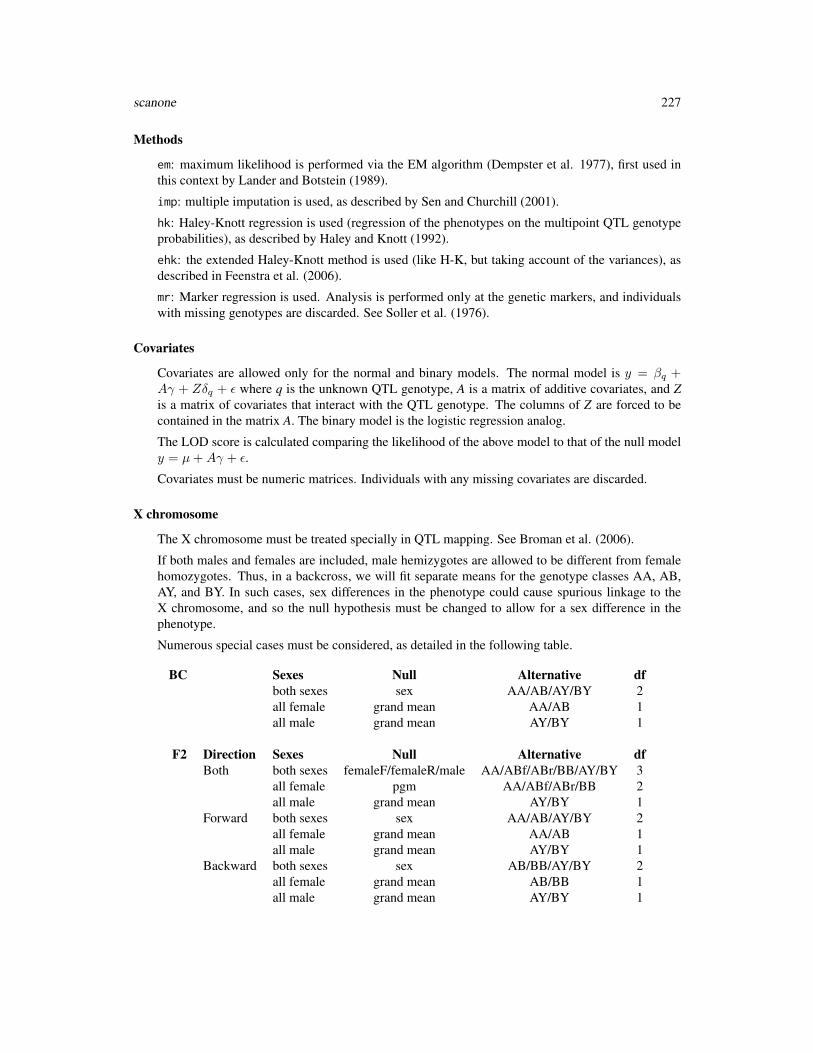
scanone 227
Methods
em: maximum likelihood is performed via the EM algorithm (Dempster et al. 1977), first used inthis context by Lander and Botstein (1989).
imp: multiple imputation is used, as described by Sen and Churchill (2001).
hk: Haley-Knott regression is used (regression of the phenotypes on the multipoint QTL genotypeprobabilities), as described by Haley and Knott (1992).
ehk: the extended Haley-Knott method is used (like H-K, but taking account of the variances), asdescribed in Feenstra et al. (2006).
mr: Marker regression is used. Analysis is performed only at the genetic markers, and individualswith missing genotypes are discarded. See Soller et al. (1976).
Covariates
Covariates are allowed only for the normal and binary models. The normal model is y = βq +Aγ + Zδq + ε where q is the unknown QTL genotype, A is a matrix of additive covariates, and Zis a matrix of covariates that interact with the QTL genotype. The columns of Z are forced to becontained in the matrix A. The binary model is the logistic regression analog.
The LOD score is calculated comparing the likelihood of the above model to that of the null modely = µ+Aγ + ε.
Covariates must be numeric matrices. Individuals with any missing covariates are discarded.
X chromosome
The X chromosome must be treated specially in QTL mapping. See Broman et al. (2006).
If both males and females are included, male hemizygotes are allowed to be different from femalehomozygotes. Thus, in a backcross, we will fit separate means for the genotype classes AA, AB,AY, and BY. In such cases, sex differences in the phenotype could cause spurious linkage to theX chromosome, and so the null hypothesis must be changed to allow for a sex difference in thephenotype.
Numerous special cases must be considered, as detailed in the following table.
BC Sexes Null Alternative dfboth sexes sex AA/AB/AY/BY 2all female grand mean AA/AB 1all male grand mean AY/BY 1
F2 Direction Sexes Null Alternative dfBoth both sexes femaleF/femaleR/male AA/ABf/ABr/BB/AY/BY 3
all female pgm AA/ABf/ABr/BB 2all male grand mean AY/BY 1
Forward both sexes sex AA/AB/AY/BY 2all female grand mean AA/AB 1all male grand mean AY/BY 1
Backward both sexes sex AB/BB/AY/BY 2all female grand mean AB/BB 1all male grand mean AY/BY 1

228 scanone
In the case that the number of degrees of freedom for the linkage test for the X chromosome is differ-ent from that for autosomes, a separate X-chromosome LOD threshold is recommended. Autosome-and X-chromosome-specific LOD thresholds may be estimated by permutation tests with scanoneby setting n.perm>0 and using perm.Xsp=TRUE.
Author(s)
Karl W Broman, <[email protected]>; Hao Wu
References
Boyartchuk, V. L., Broman, K. W., Mosher, R. E., D’Orazio S. E. F., Starnbach, M. N. and Dietrich,W. F. (2001) Multigenic control of Listeria monocytogenes susceptibility in mice. Nature Genetics27, 259–260.
Broman, K. W. (2003) Mapping quantitative trait loci in the case of a spike in the phenotype distri-bution. Genetics 163, 1169–1175.
Broman, K. W., Sen, S, Owens, S. E., Manichaikul, A., Southard-Smith, E. M. and Churchill G. A.(2006) The X chromosome in quantitative trait locus mapping. Genetics, 174, 2151–2158.
Churchill, G. A. and Doerge, R. W. (1994) Empirical threshold values for quantitative trait mapping.Genetics 138, 963–971.
Dempster, A. P., Laird, N. M. and Rubin, D. B. (1977) Maximum likelihood from incomplete datavia the EM algorithm. J. Roy. Statist. Soc. B, 39, 1–38.
Feenstra, B., Skovgaard, I. M. and Broman, K. W. (2006) Mapping quantitative trait loci by anextension of the Haley-Knott regression method using estimating equations. Genetics, 173, 2111–2119.
Haley, C. S. and Knott, S. A. (1992) A simple regression method for mapping quantitative trait lociin line crosses using flanking markers. Heredity 69, 315–324.
Kruglyak, L. and Lander, E. S. (1995) A nonparametric approach for mapping quantitative trait loci.Genetics 139, 1421–1428.
Lander, E. S. and Botstein, D. (1989) Mapping Mendelian factors underlying quantitative traitsusing RFLP linkage maps. Genetics 121, 185–199.
Sen, S. and Churchill, G. A. (2001) A statistical framework for quantitative trait mapping. Genetics159, 371–387.
Soller, M., Brody, T. and Genizi, A. (1976) On the power of experimental designs for the detectionof linkage between marker loci and quantitative loci in crosses between inbred lines. Theor. Appl.Genet. 47, 35–39.
Xu, S., and Atchley, W.R. (1996) Mapping quantitative trait loci for complex binary diseases usingline crosses. Genetics 143, 1417–1424.
See Also
plot.scanone, summary.scanone, scantwo, calc.genoprob, sim.geno, max.scanone, summary.scanoneperm,-.scanone, +.scanone

scanone 229
Examples
#################### Normal Model###################data(hyper)
# Genotype probabilities for EM and H-K## Not run: hyper <- calc.genoprob(hyper, step=2.5)
out.em <- scanone(hyper, method="em")out.hk <- scanone(hyper, method="hk")
# Summarize results: peaks above 3summary(out.em, thr=3)summary(out.hk, thr=3)
# An alternate method of summarizing:# patch them together and then summarizeout <- c(out.em, out.hk)summary(out, thr=3, format="allpeaks")
# Plot the resultsplot(out.hk, out.em)plot(out.hk, out.em, chr=c(1,4), lty=1, col=c("blue","black"))
# Imputation; first need to run sim.geno# Do just chromosomes 1 and 4, to save time## Not run: hyper.c1n4 <- sim.geno(subset(hyper, chr=c(1,4)),
step=2.5, n.draws=8)
## End(Not run)out.imp <- scanone(hyper.c1n4, method="imp")summary(out.imp, thr=3)
# Plot all three resultsplot(out.imp, out.hk, out.em, chr=c(1,4), lty=1,
col=c("red","blue","black"))
# extended Haley-Knottout.ehk <- scanone(hyper, method="ehk")plot(out.hk, out.em, out.ehk, chr=c(1,4))
# Permutation tests## Not run: permo <- scanone(hyper, method="hk", n.perm=1000)
# Threshold from the permutation testsummary(permo, alpha=c(0.05, 0.10))
# Results above the 0.05 thresholdsummary(out.hk, perms=permo, alpha=0.05)
230 scanone
##################### scan with square-root of phenotype# (Note that pheno.col can be a vector of phenotype values)####################out.sqrt <- scanone(hyper, pheno.col=sqrt(pull.pheno(hyper, 1)))plot(out.em - out.sqrt, ylim=c(-0.1,0.1),
ylab="Difference in LOD")abline(h=0, lty=2, col="gray")
##################### Stratified permutations####################extremes <- (nmissing(hyper)/totmar(hyper) < 0.5)
## Not run: operm.strat <- scanone(hyper, method="hk", n.perm=1000,perm.strata=extremes)
## End(Not run)
summary(operm.strat)
##################### X-specific permutations####################data(fake.f2)
## Not run: fake.f2 <- calc.genoprob(fake.f2, step=2.5)
# genome scanout <- scanone(fake.f2, method="hk")
# X-chr-specific permutations## Not run: operm <- scanone(fake.f2, method="hk", n.perm=1000, perm.Xsp=TRUE)
# thresholdssummary(operm)
# scanone summary with p-valuessummary(out, perms=operm, alpha=0.05, pvalues=TRUE)
#################### Non-parametric###################out.np <- scanone(hyper, model="np")summary(out.np, thr=3)

scanone 231
# Plot with previous resultsplot(out.np, chr=c(1,4), lty=1, col="green")plot(out.imp, out.hk, out.em, chr=c(1,4), lty=1,
col=c("red","blue","black"), add=TRUE)
#################### Two-part Model###################data(listeria)
## Not run: listeria <- calc.genoprob(listeria,step=2.5)
out.2p <- scanone(listeria, model="2part", upper=TRUE)summary(out.2p, thr=c(5,3,3), format="allpeaks")
# Plot all three LOD scores togetherplot(out.2p, out.2p, out.2p, lodcolumn=c(2,3,1), lty=1, chr=c(1,5,13),
col=c("red","blue","black"))
# Permutation test## Not run: permo <- scanone(listeria, model="2part", upper=TRUE,
n.perm=1000)
## End(Not run)
# Thresholdssummary(permo)
#################### Binary model###################binphe <- as.numeric(pull.pheno(listeria,1)==264)out.bin <- scanone(listeria, pheno.col=binphe, model="binary")summary(out.bin, thr=3)
# Plot LOD for binary model with LOD(p) from 2-part modelplot(out.bin, out.2p, lodcolumn=c(1,2), lty=1, col=c("black", "red"),
chr=c(1,5,13))
# Permutation test## Not run: permo <- scanone(listeria, pheno.col=binphe, model="binary",
n.perm=1000)
## End(Not run)
# Thresholdssummary(permo)
#################### Covariates###################data(fake.bc)
232 scanoneboot
## Not run: fake.bc <- calc.genoprob(fake.bc, step=2.5)
# genome scans without covariatesout.nocovar <- scanone(fake.bc)
# genome scans with covariatesac <- pull.pheno(fake.bc, c("sex","age"))ic <- pull.pheno(fake.bc, "sex")
out.covar <- scanone(fake.bc, pheno.col=1,addcovar=ac, intcovar=ic)
summary(out.nocovar, thr=3)summary(out.covar, thr=3)plot(out.covar, out.nocovar, chr=c(2,5,10))
scanoneboot Bootstrap to get interval estimate of QTL location
Description
Nonparametric bootstrap to get an estimated confidence interval for the location of a QTL, in thecontext of a single-QTL model.
Usage
scanoneboot(cross, chr, pheno.col=1, model=c("normal","binary","2part","np"),method=c("em","imp","hk","ehk","mr","mr-imp","mr-argmax"),addcovar=NULL, intcovar=NULL, weights=NULL,use=c("all.obs", "complete.obs"), upper=FALSE,ties.random=FALSE, start=NULL, maxit=4000,tol=1e-4, n.boot=1000, verbose=FALSE)
Arguments
cross An object of class cross. See read.cross for details.
chr The chromosome to investigate. Only one chromosome is allowed. (This shouldbe a character string referring to the chromosomes by name.)
pheno.col Column number in the phenotype matrix which should be used as the phenotype.One may also give a character string matching a phenotype name. Finally, onemay give a numeric vector of phenotypes, in which case it must have the lengthequal to the number of individuals in the cross, and there must be either non-integers or values < 1 or > no. phenotypes; this last case may be useful forstudying transformations.
model The phenotypic model: the usual normal model, a model for binary traits, atwo-part model or non-parametric analysis
scanoneboot 233
method Indicates whether to use the EM algorithm, imputation, Haley-Knott regression,the extended Haley-Knott method, or marker regression. Not all methods areavailable for all models. Marker regression is performed either by dropping in-dividuals with missing genotypes ("mr"), or by first filling in missing data usinga single imputation ("mr-imp") or by the Viterbi algorithm ("mr-argmax").
addcovar Additive covariates; allowed only for the normal and binary models.
intcovar Interactive covariates (interact with QTL genotype); allowed only for the normaland binary models.
weights Optional weights of individuals. Should be either NULL or a vector of lengthn.ind containing positive weights. Used only in the case model="normal".
use In the case that multiple phenotypes are selected to be scanned, this argument in-dicates whether to use all individuals, including those missing some phenotypes,or just those individuals that have data on all selected phenotypes.
upper Used only for the two-part model; if true, the "undefined" phenotype is the max-imum observed phenotype; otherwise, it is the smallest observed phenotype.
ties.random Used only for the non-parametric "model"; if TRUE, ties in the phenotypes areranked at random. If FALSE, average ranks are used and a corrected LOD scoreis calculated.
start Used only for the EM algorithm with the normal model and no covariates. IfNULL, use the usual starting values; if length 1, use random initial weights forEM; otherwise, this should be a vector of length n+1 (where n is the number ofpossible genotypes for the cross), giving the initial values for EM.
maxit Maximum number of iterations for methods "em" and "ehk".
tol Tolerance value for determining convergence for methods "em" and "ehk".
n.boot Number of bootstrap replicates.
verbose If TRUE, display information about the progress of the bootstrap.
Details
We recommend against the use of the bootstrap to derive a confidence interval for the location of aQTL; see Manichaikul et al. (2006). Use lodint or bayesint instead.
The bulk of the arguments are the same as for the scanone function. A single chromosome shouldbe indicated with the chr argument; otherwise, we focus on the first chromosome in the input crossobject.
A single-dimensional scan on the relevant chromosome is performed. We further perform a non-parametric bootstrap (sampling individuals with replacement from the available data, to create anew data set with the same size as the input cross; some individuals with be duplicated and someomitted). The same scan is performed with the resampled data; for each bootstrap replicate, westore only the location with maximum LOD score.
Use summary.scanoneboot to obtain the desired confidence interval.
Value
A vector of length n.boot, giving the estimated QTL locations in the bootstrap replicates. Theresults for the original data are included as an attribute, "results".
234 scanonevar
Author(s)
Karl W Broman, <[email protected]>
References
Manichaikul, A., Dupuis, J., Sen, S and Broman, K. W. (2006) Poor performance of bootstrapconfidence intervals for the location of a quantitative trait locus. Genetics 174, 481–489.
Visscher, P. M., Thompson, R. and Haley, C. S. (1996) Confidence intervals in QTL mapping bybootstrap. Genetics 143, 1013–1020.
See Also
scanone, summary.scanoneboot, plot.scanoneboot, lodint, bayesint
Examples
data(fake.f2)fake.f2 <- calc.genoprob(fake.f2, step=1, err=0.001)## Not run: bootoutput <- scanoneboot(fake.f2, chr=13, method="hk")
plot(bootoutput)summary(bootoutput)
scanonevar Genome scan for QTL affecting mean and/or variance
Description
Genome scan with a single QTL model for loci that can affect the variance as well as the mean.
Usage
scanonevar(cross, pheno.col=1, mean_covar=NULL, var_covar=NULL,maxit=25, tol=1e-6, quiet=TRUE)
Arguments
cross An object of class cross. See read.cross for details.
pheno.col Column number in the phenotype matrix which should be used as the pheno-type. This must be a single value (integer index or phenotype name) or a nu-meric vector of phenotype values, in which case it must have the length equalto the number of individuals in the cross, and there must be either non-integersor values < 1 or > no. phenotypes; this last case may be useful for studyingtransformations.
mean_covar Numeric matrix with covariates affecting the mean.
var_covar Numeric matrix with covariates affecting the variances.
scanonevar 235
maxit Maximum number of iterations in the algorithm to fit the model at a given posi-tion.
tol Tolerance for convergence.
quiet If FALSE, print some information about the course of the calculations.
Value
A data frame (with class "scanone", in the form output by scanone), with four columns: chro-mosome, position, the -log P-value for the mean effect, and the -log P-value for the effect on thevariance. The result is given class "scanone"
Author(s)
Lars Ronnegard and Karl Broman
References
Ronnegard, L. and Valdar W. (2011) Detecting major genetic loci controlling phenotypic variabilityin experimental crosses. Genetics 188:435-447
Ronnegard, L. and Valdar W. (2012) Recent developments in statistical methods for detecting ge-netic loci affecting phenotypic variability. BMC Genetics 13:63
See Also
scanone, summary.scanone, calc.genoprob, summary.scanoneperm
Examples
data(fake.bc)
fake.bc <- calc.genoprob(fake.bc, step=2.5)out <- scanonevar(fake.bc)color <- c("slateblue", "violetred")plot(out, lod=1:2, col=color, bandcol="gray80")legend("topright", lwd=2, c("mean", "variance"), col=color)
# use format="allpeaks" to get summary for each of mean and variance# also consider format="tabByCol" or format="tabByChr"summary(out, format="allpeaks")
# with sex and age as covariatescovar <- fake.bc$pheno[,c("sex", "age")]out.cov <- scanonevar(fake.bc, mean_covar=covar, var_covar=covar)
236 scanonevar.meanperm
scanonevar.meanperm Permutation test for mean effect in scanonevar
Description
Executes permutations of the genotypes in the mean-effect part of scanonevar
Usage
scanonevar.meanperm(cross, pheno.col=1, mean_covar=NULL, var_covar=NULL,maxit=25, tol=1e-6, n.mean.perm = 2, seed = 27517, quiet=TRUE)
Arguments
cross An object of class cross. See read.cross for details.
pheno.col Column number in the phenotype matrix which should be used as the pheno-type. This must be a single value (integer index or phenotype name) or a nu-meric vector of phenotype values, in which case it must have the length equalto the number of individuals in the cross, and there must be either non-integersor values < 1 or > no. phenotypes; this last case may be useful for studyingtransformations.
mean_covar Numeric matrix with covariates affecting the mean.
var_covar Numeric matrix with covariates affecting the variances.
maxit Maximum number of iterations in the algorithm to fit the model at a given posi-tion.
tol Tolerance for convergence.
n.mean.perm Numeric vector of length one indicates the number of permutations to execute.
seed Numeric vector of length one indicates the random seed to start the permuta-tions.
quiet If FALSE, print some information about the course of the calculations.
Value
A vector of length n.mean.perm of the maximum negative log10 p-value that resulted from eachpermutation.
scanonevar.varperm 237
scanonevar.varperm Permutation test for variance effect in scanonevar
Description
Executes permutations of the genotypes in the variance-effect part of scanonevar
Usage
scanonevar.varperm(cross, pheno.col=1, mean_covar=NULL, var_covar=NULL,maxit=25, tol=1e-6, n.var.perm = 2, seed = 27517, quiet=TRUE)
Arguments
cross An object of class cross. See read.cross for details.
pheno.col Column number in the phenotype matrix which should be used as the pheno-type. This must be a single value (integer index or phenotype name) or a nu-meric vector of phenotype values, in which case it must have the length equalto the number of individuals in the cross, and there must be either non-integersor values < 1 or > no. phenotypes; this last case may be useful for studyingtransformations.
mean_covar Numeric matrix with covariates affecting the mean.
var_covar Numeric matrix with covariates affecting the variances.
maxit Maximum number of iterations in the algorithm to fit the model at a given posi-tion.
tol Tolerance for convergence.
n.var.perm Numeric vector of length one indicates the number of permutations to execute.
seed Numeric vector of length one indicates the random seed to start the permuta-tions.
quiet If FALSE, print some information about the course of the calculations.
Value
A vector of length n.var.perm of the maximum negative log10 p-value that resulted from eachpermutation.
238 scanPhyloQTL
scanPhyloQTL Single-QTL genome scan to map QTL to a phylogenetic tree
Description
Jointly consider multiple intercrosses with a single diallelic QTL model, considering all possiblepartitions of the strains into the two QTL allele groups.
Usage
scanPhyloQTL(crosses, partitions, chr, pheno.col=1,model=c("normal", "binary"), method=c("em", "imp", "hk"),addcovar, maxit=4000, tol=0.0001, useAllCrosses=TRUE,verbose=FALSE)
Arguments
crosses A list with each component being an intercross, as an object of class cross (seeread.cross for details). The names (of the form "AB") indicate the strains inthe cross.
partitions A vector of character strings of the form "AB|CD" or "A|BCD" indicating theset of paritions of the strains into two allele groups. If missing, all partitionsshould be considered.
chr Optional vector indicating the chromosomes for which LOD scores should becalculated. This should be a vector of character strings referring to chromo-somes by name; numeric values are converted to strings. Refer to chromosomeswith a preceding - to have all chromosomes but those considered. A logical(TRUE/FALSE) vector may also be used.
pheno.col Column number in the phenotype matrix which should be used as the pheno-type. This can be a vector of integers; for methods "hk" and "imp" this can beconsiderably faster than doing them one at a time. One may also give a char-acter strings matching the phenotype names. Finally, one may give a numericvector of phenotypes, in which case it must have the length equal to the numberof individuals in the cross, and there must be either non-integers or values < 1or > no. phenotypes; this last case may be useful for studying transformations.
model The phenotype model: the usual normal model or a model for binary traitsmethod Indicates whether to use the EM algorithm, imputation, or Haley-Knott regres-
sion.addcovar Optional set of additive covariates to include in the analysis, as a list with the
same length as crosses. They must be numeric vectors or matrices, as forscanone.
maxit Maximum number of iterations for method "em".tol Tolerance value for determining convergence for method "em".useAllCrosses If TRUE, use all crosses in the analysis of all partitions, with crosses not segre-
gating the QTL included in the estimation of the residual variance.verbose If TRUE, print information about progress.
scanPhyloQTL 239
Details
The aim is to jointly consider multiple intercrosses to not just map QTL but to also, under theassumption of a single diallelic QTL, identify the set of strains with each QTL allele.
For each partition (of the strains into two groups) that is under consideration, we pull out the setof crosses that are segregating the QTL, re-code the alleles, and combine the crosses into one largecross. Crosses not segregating the QTL are also used, though with no QTL effects.
Additive covariate indicators for the crosses are included in the analysis, to allow for the possibilitythat there are overall shifts in the phenotypes between crosses.
Value
A data frame, as for the output of scanone, though with LOD score columns for each partition thatis considered. The result is given class "scanPhyloQTL".
Author(s)
Karl W Broman, <[email protected]>
References
Broman, K. W., Kim, S., An\’e, C. and Payseur, B. A. Mapping quantitative trait loci to a phyloge-netic tree. In preparation.
See Also
plot.scanPhyloQTL, summary.scanPhyloQTL, max.scanPhyloQTL, inferredpartitions, simPhyloQTL
Examples
# example map; drop X chromosomedata(map10)map10 <- map10[1:19]
# simulate datax <- simPhyloQTL(4, partition="AB|CD", crosses=c("AB", "AC", "AD"),
map=map10, n.ind=150,model=c(1, 50, 0.5, 0))
# run calc.genoprob on each cross## Not run: x <- lapply(x, calc.genoprob, step=2)
# scan genome, at each position trying all possible partitionsout <- scanPhyloQTL(x, method="hk")
# maximum peakmax(out, format="lod")
240 scanqtl
# approximate posterior probabilities at peakmax(out, format="postprob")
# all peaks above a threshold for LOD(best) - LOD(2nd best)summary(out, threshold=1, format="lod")
# all peaks above a threshold for LOD(best), showing approx post'r probsummary(out, format="postprob", threshold=3)
# plot resultsplot(out)
scanqtl General QTL scan
Description
Performs a multiple QTL scan for specified chromosomes and positions or intervals, with the pos-sible inclusion of QTL-QTL interactions and/or covariates.
Usage
scanqtl(cross, pheno.col=1, chr, pos, covar=NULL, formula,method=c("imp","hk"), model=c("normal", "binary"),incl.markers=FALSE, verbose=TRUE, tol=1e-4, maxit=1000,forceXcovar=FALSE)
Arguments
cross An object of class cross. See read.cross for details.
pheno.col Column number in the phenotype matrix to be used as the phenotype. One mayalso give a character string matching a phenotype name. Finally, one may givea numeric vector of phenotypes, in which case it must have the length equal tothe number of individuals in the cross, and there must be either non-integersor values < 1 or > no. phenotypes; this last case may be useful for studyingtransformations.
chr Vector indicating the chromosome for each QTL. (These should be characterstrings referring to the chromosomes by name.)
pos List indicating the positions or intervals on the chromosome to be scanned. Eachelement should be either a single number (for a specific position) or a pair ofnumbers (for an interval).
covar A matrix or data.frame of covariates. These must be strictly numeric.
formula An object of class formula indicating the model to be fitted. (It can also be thecharacter string representation of a formula.) QTLs are indicated as Q1, Q2, etc.Covariates are indicated by their names in covar.
method Indicates whether to use multiple imputation or Haley-Knott regression.

scanqtl 241
model The phenotype model: the usual model or a model for binary traitsincl.markers If FALSE, do calculations only at points on an evenly spaced grid. If calc.genoprob
or sim.geno were run with stepwidth="variable" or stepwidth="max", weforce incl.markers=TRUE.
verbose If TRUE, give feedback about progress.tol Tolerance for convergence for the binary trait model.maxit Maximum number of iterations for fitting the binary trait model.forceXcovar If TRUE, force inclusion of X-chr-related covariates (like sex and cross direc-
tion).
Details
The formula is used to specified the model to be fit. In the formula, use Q1, Q2, etc., or q1, q2, etc.,to represent the QTLs, and the column names in the covariate data frame to represent the covariates.
We enforce a hierarchical structure on the model formula: if a QTL or covariate is in involved in aninteraction, its main effect are also be included.
Only the interaction terms need to be specifed in the formula. The main effects of all input QTLs(as specified by chr and pos) and covariates (as specifed by covar) will be included by default.For example, if the formula is y~Q1*Q2*Sex, and there are three elements in input chr and posand Sex is one of the column names for input covariates, the formula used in genome scan will bey ~ Q1 + Q2 + Q3 + Sex + Q1:Q2 + Q1:Sex + Q2:Sex + Q1:Q2:Sex.
The input pos is a list or vector to specify the position/range of the input chromosomes to bescanned. If it is a vector, it gives the precise positions of the QTL on the chromosomes. If it is a list,it will contain either the precise positions or a range on the chromosomes. For example, considerthe case that the input chr = c(1, 6, 13). If pos = c(9.8, 34.0, 18.6), it means tofit a model with QTL on chromosome 1 at 9.8cM, chromosome 6 at 34cM and chromosome 13 at18.6cM. If pos = list(c(5,15), c(30,36), 18), it means to scan chromosome 1 from 5cM to15cM, chromosome 6 from 30cM to 36cM, fix the QTL on chromosome 13 at 18cM.
Value
An object of class scanqtl. It is a multi-dimensional array of LOD scores, with the number ofdimension equal to the number of QTLs specifed.
Author(s)
Hao Wu
References
Haley, C. S. and Knott, S. A. (1992) A simple regression method for mapping quantitative trait lociin line crosses using flanking markers. Heredity 69, 315–324.
Sen, S. and Churchill, G. A. (2001) A statistical framework for quantitative trait mapping. Genetics159, 371–387.
See Also
fitqtl, makeqtl, refineqtl

242 scantwo
Examples
data(fake.f2)
# take out several QTLsqc <- c(1, 8, 13)fake.f2 <- subset(fake.f2, chr=qc)
# imputate genotypes
fake.f2 <- calc.genoprob(fake.f2, step=5, err=0.001)
# 2-dimensional genome scan with additive 3-QTL modelpos <- list(c(15,35), c(45,65), 28)result <- scanqtl(fake.f2, pheno.col=1, chr=qc, pos=pos,
formula=y~Q1+Q2+Q3, method="hk")
# image of the results# chr locationschr1 <- as.numeric(matrix(unlist(strsplit(colnames(result),"@")),
ncol=2,byrow=TRUE)[,2])chr8 <- as.numeric(matrix(unlist(strsplit(rownames(result),"@")),
ncol=2,byrow=TRUE)[,2])# image plotimage(chr1, chr8, t(result), las=1, col=rev(rainbow(256,start=0,end=2/3)))
# do the same, allowing the QTLs on chr 1 and 13 to interactresult2 <- scanqtl(fake.f2, pheno.col=1, chr=qc, pos=pos,
formula=y~Q1+Q2+Q3+Q1:Q3, method="hk")# image plotimage(chr1, chr8, t(result2), las=1, col=rev(rainbow(256,start=0,end=2/3)))
scantwo Two-dimensional genome scan with a two-QTL model
Description
Perform a two-dimensional genome scan with a two-QTL model, with possible allowance for co-variates.
Usage
scantwo(cross, chr, pheno.col=1, model=c("normal","binary"),method=c("em","imp","hk","mr","mr-imp","mr-argmax"),addcovar=NULL, intcovar=NULL, weights=NULL,use=c("all.obs", "complete.obs"),incl.markers=FALSE, clean.output=FALSE,clean.nmar=1, clean.distance=0,maxit=4000, tol=1e-4,verbose=TRUE, n.perm, perm.Xsp=FALSE, perm.strata=NULL,assumeCondIndep=FALSE, batchsize=250, n.cluster=1)
scantwo 243
Arguments
cross An object of class cross. See read.cross for details.
chr Optional vector indicating the chromosomes for which LOD scores should becalculated. This should be a vector of character strings referring to chromo-somes by name; numeric values are converted to strings. Refer to chromosomeswith a preceding - to have all chromosomes but those considered. A logical(TRUE/FALSE) vector may also be used.
pheno.col Column number in the phenotype matrix which should be used as the pheno-type. This can be a vector of integers; for methods "hk" and "imp" this can beconsiderably faster than doing them one at a time. One may also give characterstrings matching the phenotype names. Finally, one may give a numeric vectorof phenotypes, in which case it must have the length equal to the number ofindividuals in the cross, and there must be either non-integers or values < 1 or >no. phenotypes; this last case may be useful for studying transformations.
model The phenotype model: the usual normal model or a model for binary traits.
method Indicates whether to use the the EM algorithm, imputation, Haley-Knott regres-sion, or marker regression. Marker regression is performed either by droppingindividuals with missing genotypes ("mr"), or by first filling in missing data us-ing a single imputation ("mr-imp") or by the Viterbi algorithm ("mr-argmax").
addcovar Additive covariates.
intcovar Interactive covariates (interact with QTL genotype).
weights Optional weights of individuals. Should be either NULL or a vector of lengthn.ind containing positive weights. Used only in the case model="normal".
use In the case that multiple phenotypes are selected to be scanned, this argument in-dicates whether to use all individuals, including those missing some phenotypes,or just those individuals that have data on all selected phenotypes.
incl.markers If FALSE, do calculations only at points on an evenly spaced grid. If calc.genoprobor sim.geno were run with stepwidth="variable" or stepwidth="max", weforce incl.markers=TRUE.
clean.output If TRUE, clean the output with clean.scantwo, replacing LOD scores for pairsof positions that are not well separated with 0. In permutations, this will bedone for each permutation replicate. This can be important for the case ofmethod="em", as there can be difficulty with algorithm convergence in theseregions.
clean.nmar If clean.output=TRUE, this is the number of markers that must separate twopositions.
clean.distance If clean.output=TRUE, this is the cM distance that must separate two positions.
maxit Maximum number of iterations; used only with method "em".
tol Tolerance value for determining convergence; used only with method "em".
verbose If TRUE, display information about the progress of calculations. For method"em", if verbose is an integer above 1, further details on the progress of thealgorithm will be displayed.
n.perm If specified, a permutation test is performed rather than an analysis of the ob-served data. This argument defines the number of permutation replicates.

244 scantwo
perm.Xsp If n.perm > 0, so that a permutation test will be performed, this indicates whetherseparate permutations should be performed for the autosomes and the X chro-mosome, in order to get an X-chromosome-specific LOD threshold. In this case,additional permutations are performed for the X chromosome.
perm.strata If n.perm > 0, this may be used to perform a stratified permutation test. Thisshould be a vector with the same number of individuals as in the cross data.Unique values indicate the individual strata, and permutations will be performedwithin the strata.
assumeCondIndep
If TRUE, assume conditional independence of QTL genotypes given markergenotypes. This is an approximation, but it may speed things up.
batchsize The number of phenotypes (or permutations) to be run as a batch; used only formethods "hk" and "imp".
n.cluster If the package snow is available and n.perm > 0, permutations are run in parallelusing this number of nodes.
Details
Standard interval mapping (method="em") and Haley-Knott regression (method="hk") require thatmultipoint genotype probabilities are first calculated using calc.genoprob. The imputation methoduses the results of sim.geno.
The method "em" is standard interval mapping by the EM algorithm (Dempster et al. 1977; Landerand Botstein 1989). Marker regression (method="mr") is simply linear regression of phenotypeson marker genotypes (individuals with missing genotypes are discarded). Haley-Knott regression(method="hk") uses the regression of phenotypes on multipoint genotype probabilities. The impu-tation method (method="imp") uses the pseudomarker algorithm described by Sen and Churchill(2001).
Individuals with missing phenotypes are dropped.
In the presence of covariates, the full model is
y = µ+ βq1 + βq2 + βq1×q2 +Aγ + Zδq1 + Zδq2 + Zδq1×q2 + ε
where q1 and q2 are the unknown QTL genotypes at two locations, A is a matrix of covariates, andZ is a matrix of covariates that interact with QTL genotypes. The columns of Z are forced to becontained in the matrix A.
The above full model is compared to the additive QTL model,
y = µ+ βq1 + βq2 +Aγ + Zδq1 + Zδq2 + ε
and also to the null model, with no QTL,
y = µ+Aγ + ε
In the case that n.perm is specified, the R function scantwo is called repeatedly.
For model="binary", a logistic regression model is used.
scantwo 245
Value
If n.perm is missing, the function returns a list with class "scantwo" and containing three compo-nents. The first component is a matrix of dimension [tot.pos x tot.pos]; the upper triangle containsthe LOD scores for the additive model, and the lower triangle contains the LOD scores for the fullmodel. The diagonal contains the results of scanone. The second component of the output is adata.frame indicating the locations at which the two-QTL LOD scores were calculated. The firstcolumn is the chromosome identifier, the second column is the position in cM, the third column isa 1/0 indicator for ease in later pulling out only the equally spaced positions, and the fourth columnindicates whether the position is on the X chromosome or not. The final component is a version ofthe results of scanone including sex and/or cross direction as additive covariates, which is neededfor a proper calculation of conditional LOD scores.
If n.perm is specified, the function returns a list with six different LOD scores from each of thepermutation replicates. First, the maximum LOD score for the full model (two QTLs plus an in-teraction). Second, for each pair of chromosomes, we take the difference between the full LODand the maximum single-QTL LOD for those two chromosomes, and then maximize this acrosschromosome pairs. Third, for each pair of chromosomes we take the difference between the maxi-mum full LOD and the maximum additive LOD, and then maximize this across chromosome pairs.Fourth, the maximum LOD score for the additive QTL model. Fifth, for each pair of chromosomes,we take the difference between the additive LOD and the maximum single-QTL LOD for those twochromosomes, and then maximize this across chromosome pairs. Finally, the maximum single-QTLLOD score (that is, from a single-QTL scan). The latter is not used in summary.scantwo, but doesget calculated at each permutation, so we include it for the sake of completeness.
If n.perm is specified and perm.Xsp=TRUE, the result is a list with the permutation results for theregions A:A, A:X, and X:X, each of which is a list with the six different LOD scores. Independentpermutations are performed in each region, n.perm is the number of permutations for the A:Aregion; additional permutations are are used for the A:X and X:X parts, as estimates of quantilesfarther out into the tails are needed.
X chromosome
The X chromosome must be treated specially in QTL mapping.
As in scanone, if both males and females are included, male hemizygotes are allowed to be differentfrom female homozygotes, and the null hypothesis must be changed in order to ensure that sex- orpgm-differences in the phenotype do not results in spurious linkage to the X chromosome. (See thehelp file for scanone.)
If n.perm is specified and perm.Xsp=TRUE, X-chromosome-specific permutations are performed, toobtain separate thresholds for the regions A:A, A:X, and X:X.
Author(s)
Karl W Broman, <[email protected]>; Hao Wu
References
Churchill, G. A. and Doerge, R. W. (1994) Empirical threshold values for quantitative trait mapping.Genetics 138, 963–971.
246 scantwo
Dempster, A. P., Laird, N. M. and Rubin, D. B. (1977) Maximum likelihood from incomplete datavia the EM algorithm. J. Roy. Statist. Soc. B, 39, 1–38.
Haley, C. S. and Knott, S. A. (1992) A simple regression method for mapping quantitative trait lociin line crosses using flanking markers. Heredity 69, 315–324.
Lander, E. S. and Botstein, D. (1989) Mapping Mendelian factors underlying quantitative traitsusing RFLP linkage maps. Genetics 121, 185–199.
Sen, S. and Churchill, G. A. (2001) A statistical framework for quantitative trait mapping. Genetics159, 371–387.
Soller, M., Brody, T. and Genizi, A. (1976) On the power of experimental designs for the detectionof linkage between marker loci and quantitative loci in crosses between inbred lines. Theor. Appl.Genet. 47, 35–39.
See Also
plot.scantwo, summary.scantwo, scanone, max.scantwo, summary.scantwoperm, c.scantwoperm
Examples
data(fake.f2)
fake.f2 <- calc.genoprob(fake.f2, step=5)out.2dim <- scantwo(fake.f2, method="hk")plot(out.2dim)
# permutations
## Not run: permo.2dim <- scantwo(fake.f2, method="hk", n.perm=1000)summary(permo.2dim, alpha=0.05)
# summary with p-valuessummary(out.2dim, perms=permo.2dim, pvalues=TRUE,
alphas=c(0.05, 0.10, 0.10, 0.05, 0.10))
# covariatesdata(fake.bc)
fake.bc <- calc.genoprob(fake.bc, step=10)
ac <- pull.pheno(fake.bc, c("sex","age"))ic <- pull.pheno(fake.bc, "sex")
out <- scantwo(fake.bc, method="hk", pheno.col=1,addcovar=ac, intcovar=ic)
plot(out)

scantwopermhk 247
scantwopermhk Permutation test for 2d genome scan by Haley-Knott regression
Description
Perform a permutation test with a two-dimensional genome scan with a two-QTL model, withpossible allowance for additive covariates, by Haley-Knott regression.
Usage
scantwopermhk(cross, chr, pheno.col=1,addcovar=NULL, weights=NULL, n.perm=1,batchsize=1000,perm.strata=NULL, perm.Xsp=NULL,verbose=FALSE, assumeCondIndep=FALSE)
Arguments
cross An object of class cross. See read.cross for details.chr Optional vector indicating the chromosomes for which LOD scores should be
calculated. This should be a vector of character strings referring to chromo-somes by name; numeric values are converted to strings. Refer to chromosomeswith a preceding - to have all chromosomes but those considered. A logical(TRUE/FALSE) vector may also be used.
pheno.col Column number in the phenotype matrix which should be used as the phenotype.This should be a single value (numeric index or character string for a phenotypename), but it may also be a vector of numeric values with length equal to thenumber of individuals in the cross, in which case it is taken to be a vector ofindividuals’ phenotypes.
addcovar Additive covariates.weights Optional weights of individuals. Should be either NULL or a vector of length
n.ind containing positive weights. Used only in the case model="normal".n.perm Number of permutation replicates.batchsize If n.perm > batchsize, permutations will be run in batches of no more than
batchsize permutations.perm.strata Used to perform a stratified permutation test. This should be a vector with the
same number of individuals as in the cross data. Unique values indicate theindividual strata, and permutations will be performed within the strata.
perm.Xsp If TRUE, run separate permutations for A:A, A:X, and X:X. In this case, n.permrefers to the number of permutations for the A:A part; more permutations areused for the A:X and X:X parts, as estimates of quantiles farther out into thetails are needed.
verbose If TRUE, display information about the progress of calculations.assumeCondIndep
If TRUE, assume conditional independence of QTL genotypes given markergenotypes. This is an approximation, but it may speed things up.
248 scantwopermhk
Details
This is a scaled-back version of the permutation test provided by scantwo: only for a normal modelwith Haley-Knott regression, and not allowing interactive covariates.
This is an attempt to speed things up and attentuate the memory usage problems in scantwo.
In the case of perm.Xsp=TRUE (X-chr-specific thresholds), we use a stratified permutation test,stratified by sex and cross-direction.
Value
A list with six different LOD scores from each of the permutation replicates. First, the maximumLOD score for the full model (two QTLs plus an interaction). Second, for each pair of chromo-somes, we take the difference between the full LOD and the maximum single-QTL LOD for thosetwo chromosomes, and then maximize this across chromosome pairs. Third, for each pair of chro-mosomes we take the difference between the maximum full LOD and the maximum additive LOD,and then maximize this across chromosome pairs. Fourth, the maximum LOD score for the additiveQTL model. Fifth, for each pair of chromosomes, we take the difference between the additive LODand the maximum single-QTL LOD for those two chromosomes, and then maximize this acrosschromosome pairs. Finally, the maximum single-QTL LOD score (that is, from a single-QTL scan).The latter is not used in summary.scantwoperm, but does get calculated at each permutation, so weinclude it for the sake of completeness.
If perm.Xsp=TRUE, this is a list of lists, for the A:A, A:X, and X:X sections, each being a list asdescribed above.
Author(s)
Karl W Broman, <[email protected]>; Hao Wu
References
Churchill, G. A. and Doerge, R. W. (1994) Empirical threshold values for quantitative trait mapping.Genetics 138, 963–971.
Haley, C. S. and Knott, S. A. (1992) A simple regression method for mapping quantitative trait lociin line crosses using flanking markers. Heredity 69, 315–324.
See Also
scantwo, plot.scantwoperm, summary.scantwoperm, c.scantwoperm
Examples
data(fake.f2)
fake.f2 <- calc.genoprob(fake.f2, step=5)operm <- scantwopermhk(fake.f2, n.perm=2)summary(operm, alpha=0.05)
shiftmap 249
shiftmap Shift starting points in genetic maps
Description
Shift starting points in a genetic map to a set of defined positions
Usage
shiftmap(object, offset=0)
Arguments
object An object of class cross (see read.cross for details) or map (see sim.map fordetails).
offset Defines the starting position for each chromosome. This should be a single value(to be used for all chromosomes) or a vector with length equal to the number ofchromosomes, defining individual starting positions for each chromosome. Fora sex-specific map (as in a 4-way cross), we use the same offset for both themale and female maps.
Value
If the input is a map object, a map object is returned; if the input is a cross object, a cross object isreturned. In either case, the positions of markers are shifted so that the starting positions are as inoffset.
Author(s)
Karl W Broman, <[email protected]>
See Also
replace.map, est.map
Examples
data(hyper)shiftedhyper <- shiftmap(hyper, offset=0)par(mfrow=c(1,2))plotMap(hyper, shift=FALSE, alternate.chrid=TRUE)plotMap(shiftedhyper, shift=FALSE, alternate.chrid=TRUE)
250 sim.cross
sim.cross Simulate a QTL experiment
Description
Simulates data for a QTL experiment using a model in which QTLs act additively.
Usage
sim.cross(map, model=NULL, n.ind=100,type=c("f2", "bc", "4way", "risib", "riself","ri4sib", "ri4self", "ri8sib", "ri8self", "bcsft"),error.prob=0, missing.prob=0, partial.missing.prob=0,keep.qtlgeno=TRUE, keep.errorind=TRUE, m=0, p=0,
map.function=c("haldane","kosambi","c-f","morgan"),founderGeno, random.cross=TRUE, ...)
Arguments
map A list whose components are vectors containing the marker locations on each ofthe chromosomes.
model A matrix where each row corresponds to a different QTL, and gives the chro-mosome number, cM position and effects of the QTL.
n.ind Number of individuals to simulate.
type Indicates whether to simulate an intercross (f2), a backcross (bc), a phase-known 4-way cross (4way), or recombinant inbred lines (by selfing or by sib-mating, and with the usual 2 founder strains or with 4 or 8 founder strains).
error.prob The genotyping error rate.
missing.prob The rate of missing genotypes.partial.missing.prob
When simulating an intercross or 4-way cross, this gives the rate at which mark-ers will be incompletely informative (i.e., dominant or recessive).
keep.qtlgeno If TRUE, genotypes for the simulated QTLs will be included in the output.
keep.errorind If TRUE, and if error.prob > 0, the identity of genotyping errors will beincluded in the output.
m Interference parameter; a non-negative integer. 0 corresponds to no interference.
p Probability that a chiasma comes from the no-interference mechanism
map.function Indicates whether to use the Haldane, Kosambi, Carter-Falconer, or Morgan mapfunction when converting genetic distances into recombination fractions.
founderGeno For 4- or 8-way RIL, the genotype data of the founder strains, as a list whosecomponents are numeric matrices (no. markers x no. founders), one for eachchromosome.
sim.cross 251
random.cross For 4- or 8-way RIL, indicates whether the order of the founder strains shouldbe randomized, independently for each RIL, or whether all RIL be derivedfrom a common cross. In the latter case, for a 4-way RIL, the cross wouldbe (AxB)x(CxD).
... For type = "bcsft", additional arguments passed to sim.cross.bcsft.
Details
Meiosis is assumed to follow the Stahl model for crossover interference (see the references, below),of which the no interference model and the chi-square model are special cases. Chiasmata on thefour-strand bundle are a superposition of chiasmata from two different mechanisms. With probabil-ity p, they arise by a mechanism exhibiting no interference; the remainder come from a chi-squaremodel with inteference parameter m. Note that m=0 corresponds to no interference, and with p=0,one gets a pure chi-square model.
If a chromosomes has class X, it is assumed to be the X chromosome, and is assumed to be segregat-ing in the cross. Thus, in an intercross, it is segregating like a backcross chromosome. In a 4-waycross, a second phenotype, sex, will be generated.
QTLs are assumed to act additively, and the residual phenotypic variation is assumed to be normallydistributed with variance 1.
For a backcross, the effect of a QTL is a single number corresponding to the difference between thehomozygote and the heterozygote.
For an intercross, the effect of a QTL is a pair of numbers, (a, d), where a is the additive effect (halfthe difference between the homozygotes) and d is the dominance deviation (the difference betweenthe heterozygote and the midpoint between the homozygotes).
For a four-way cross, the effect of a QTL is a set of three numbers, (a, b, c), where, in the case ofone QTL, the mean phenotype, conditional on the QTL genotyping being AC, BC, AD or BD, is a,b, c or 0, respectively.
Value
An object of class cross. See read.cross for details.
If keep.qtlgeno is TRUE, the cross object will contain a component qtlgeno which is a matrixcontaining the QTL genotypes (with complete data and no errors), coded as in the genotype data.
If keep.errorind is TRUE and errors were simulated, each component of geno will each containa matrix errors, with 1’s indicating simulated genotyping errors.
Recombinant inbred lines
In the simulation of recombinant inbred lines (RIL), we simulate a single individual from each line,and no phenotypes are simulated (so the argument model is ignored).
The types riself and risib are the usual two-way RIL.
The types ri4self, ri4sib, ri8self, and ri8sib are RIL by selfing or sib-mating derived fromfour or eight founding parental strains.
For the 4- and 8-way RIL, one must include the genotypes of the founding individuals; these maybe simulated with simFounderSnps. Also, the output cross will contain a component cross, which
252 sim.cross
is a matrix with rows corresponding to RIL and columns corresponding to the founders, indicatingorder of the founder strains in the crosses used to generate the RIL.
The coding of genotypes in 4- and 8-way RIL is rather complicated. It is a binary encoding of whichfounder strains’ genotypes match the RIL’s genotype at a marker, and not that this is specific to theorder of the founders in the crosses used to generate the RIL. For example, if an RIL generatedfrom 4 founders has the 1 allele at a SNP, and the four founders have SNP alleles 0, 1, 0, 1, thenthe RIL allele matches that of founders B and D. If the RIL was derived by the cross (AxB)x(CxD),then the RIL genotype would be encoded 22−1 + 23−1 = 6. If the cross was derived by the cross(DxA)x(CxB), then the RIL genotype would be encoded 21−1 + 24−1 = 9. These get reorganizedafter calls to calc.genoprob, sim.geno, or argmax.geno, and this approach simplifies the hiddenMarkov model (HMM) code.
For the 4- and 8-way RIL, genotyping errors are simulated only if the founder genotypes are 0/1SNPs.
Author(s)
Karl W Broman, <[email protected]>
References
Copenhaver, G. P., Housworth, E. A. and Stahl, F. W. (2002) Crossover interference in arabidopsis.Genetics 160, 1631–1639.
Foss, E., Lande, R., Stahl, F. W. and Steinberg, C. M. (1993) Chiasma interference as a function ofgenetic distance. Genetics 133, 681–691.
Zhao, H., Speed, T. P. and McPeek, M. S. (1995) Statistical analysis of crossover interference usingthe chi-square model. Genetics 139, 1045–1056.
Broman, K. W. (2005) The genomes of recombinant inbred lines Genetics 169, 1133–1146.
Teuscher, F. and Broman, K. W. (2007) Haplotype probabilities for multiple-strain recombinantinbred lines. Genetics 175, 1267–1274.
See Also
sim.map, read.cross, fake.f2, fake.bc fake.4way, simFounderSnps
Examples
# simulate a genetic mapmap <- sim.map()
### simulate 250 intercross individuals with 2 QTLsfake <- sim.cross(map, type="f2", n.ind=250,
model = rbind(c(1,45,1,1),c(5,20,0.5,-0.5)))
### simulate 100 backcross individuals with 3 QTL# a 10-cM map model after the mousedata(map10)
sim.geno 253
fakebc <- sim.cross(map10, type="bc", n.ind=100,model=rbind(c(1,45,1), c(5,20,1), c(5,50,1)))
### simulate 8-way RIL by sibling mating# get lengths from the above 10-cM mapL <- ceiling(sapply(map10, max))
# simulate a 1 cM mapthemap <- sim.map(L, n.mar=L+1, eq.spacing=TRUE)
# simulate founder genotypespg <- simFounderSnps(themap, "8")
# simulate the 8-way RIL by sib mating (256 lines)ril <- sim.cross(themap, n.ind=256, type="ri8sib", founderGeno=pg)
sim.geno Simulate genotypes given observed marker data
Description
Uses the hidden Markov model technology to simulate from the joint distribution Pr(g | O) whereg is the underlying genotype vector and O is the observed multipoint marker data, with possibleallowance for genotyping errors.
Usage
sim.geno(cross, n.draws=16, step=0, off.end=0, error.prob=0.0001,map.function=c("haldane","kosambi","c-f","morgan"),stepwidth=c("fixed", "variable", "max"))
Arguments
cross An object of class cross. See read.cross for details.
n.draws Number of simulation replicates to perform.
step Maximum distance (in cM) between positions at which the simulated genotypeswill be drawn, though for step=0, genotypes are drawn only at the marker loca-tions.
off.end Distance (in cM) past the terminal markers on each chromosome to which thegenotype simulations will be carried.
error.prob Assumed genotyping error rate used in the calculation of the penetrance Pr(observedgenotype | true genotype).
map.function Indicates whether to use the Haldane, Kosambi, Carter-Falconer, or Morgan mapfunction when converting genetic distances into recombination fractions.
254 sim.map
stepwidth Indicates whether the intermediate points should with fixed or variable stepsizes. We recommend using "fixed"; "variable" is included for the qtlbimpackage (http://www.ssg.uab.edu/qtlbim). The "max" option inserts theminimal number of intermediate points so that the maximum distance betweenpoints is step.
Details
After performing the forward-backward equations, we draw fromPr(g1 = v|O) and thenPr(gk+1 =v|O, gk = u).
In the case of the 4-way cross, with a sex-specific map, we assume a constant ratio of female:malerecombination rates within the inter-marker intervals.
Value
The input cross object is returned with a component, draws, added to each component of cross$geno.This is an array of size [n.ind x n.pos x n.draws] where n.pos is the number of positions at whichthe simulations were performed and n.draws is the number of replicates. Attributes "error.prob","step", and "off.end" are set to the values of the corresponding arguments, for later reference.
Author(s)
Karl W Broman, <[email protected]>
See Also
calc.genoprob, argmax.geno
Examples
data(fake.f2)
fake.f2 <- sim.geno(fake.f2, step=2, n.draws=8)
sim.map Simulate a genetic map
Description
Simulate the positions of markers on a genetic map.
Usage
sim.map(len=rep(100,20), n.mar=10, anchor.tel=TRUE,include.x=TRUE, sex.sp=FALSE, eq.spacing=FALSE)

sim.map 255
Arguments
len A vector specifying the chromosome lengths (in cM)
n.mar A vector specifying the number of markers per chromosome.
anchor.tel If true, markers at the two telomeres will always be included, so if n.mar = 1 or2, we’ll give just the two telomeric markers.
include.x Indicates whether the last chromosome should be considered the X chromo-some.
sex.sp Indicates whether to create sex-specific maps, in which case the output will bea vector of 2-row matrices, with rows corresponding to the maps for the twosexes.
eq.spacing If TRUE, markers will be equally spaced.
Details
Aside from the telomeric markers, marker positions are simulated as iid Uniform(0, L). If len orn.mar has just one element, it is expanded to the length of the other argument. If they both havejust one element, only one chromosome is simulated.
If eq.spacing is TRUE, markers are equally spaced between 0 and L. If anchor.tel is FALSE,telomeric markers are not included.
Value
A list of vectors, each specifying the locations of the markers. Each component of the list is givenclass A or X, according to whether it is autosomal or the X chromosome.
Author(s)
Karl W Broman, <[email protected]>
See Also
sim.cross, plotMap, replace.map, pull.map
Examples
# simulate 4 autosomes, each with 10 markersmap <- sim.map(c(100,90,80,40), 10, include.x=FALSE)plotMap(map)
# equally spaced markersmap2 <- sim.map(c(100,90,80,40), 10, include.x=FALSE, eq.spacing=TRUE)plot(map2)

256 simFounderSnps
simFounderSnps Simulate founder SNPs for a multiple-strain RIL
Description
Simulate genotype data for the founding strains for a panel of multiple-strain RIL.
Usage
simFounderSnps(map, n.str=c("4","8"), pat.freq)
Arguments
map A list whose components are vectors containing the marker locations on each ofthe chromosomes.
n.str Number of founding strains (4 or 8).
pat.freq Frequency of SNP genotype patterns in the founder (a vector of length n.str/2+ 1): (monoallelic, SNP unique to one founder, SNP present in 2 founders, [and,for the case of 8 founders, SNP in 3/8 founders, SNP in 4/8 founders].)
Details
The SNPs are simulated to be in linkage equilibrium.
Value
A vector of the same length as there are chromosomes in map, with each component being a matrixof 0’s and 1’s, of dim n.str x n.mar.
Author(s)
Karl W Broman, <[email protected]>
See Also
sim.map, sim.cross
Examples
data(map10)x <- simFounderSnps(map10, "8", c(0, 0.5, 0.2, 0.2, 0.1))
simPhyloQTL 257
simPhyloQTL Simulate a set of intercrosses for a single diallelic QTL
Description
Simulate a set of intercrosses with a single diallelic QTL.
Usage
simPhyloQTL(n.taxa=3, partition, crosses, map, n.ind=100, model,error.prob=0, missing.prob=0, partial.missing.prob=0,keep.qtlgeno=FALSE, keep.errorind=TRUE, m=0, p=0,
map.function=c("haldane","kosambi","c-f","morgan"))
Arguments
n.taxa Number of taxa (i.e., strains).
partition A vector of character strings of the form "AB|CD" or "A|BCD" indicating, foreach QTL, which taxa have which allele. If missing, simulate under the nullhypothesis of no QTL.
crosses A vector of character strings indicating the crosses to do (for the form "AB","AC", etc.). These will be sorted and then only unique ones used. If missing, allcrosses will be simulated.
map A list whose components are vectors containing the marker locations on each ofthe chromosomes.
n.ind The number of individuals in each cross. If length 1, all crosses will havethe same number of individuals; otherwise the length should be the same ascrosses.
model A matrix where each row corresponds to a different QTL, and gives the chro-mosome number, cM position and effects of the QTL (assumed to be the samein each cross in which the QTL is segregating).
error.prob The genotyping error rate.
missing.prob The rate of missing genotypes.partial.missing.prob
When simulating an intercross or 4-way cross, this gives the rate at which mark-ers will be incompletely informative (i.e., dominant or recessive).
keep.qtlgeno If TRUE, genotypes for the simulated QTLs will be included in the output.
keep.errorind If TRUE, and if error.prob > 0, the identity of genotyping errors will beincluded in the output.
m Interference parameter; a non-negative integer. 0 corresponds to no interference.
p Probability that a chiasma comes from the no-interference mechanism
map.function Indicates whether to use the Haldane, Kosambi, Carter-Falconer, or Morgan mapfunction when converting genetic distances into recombination fractions.
258 simPhyloQTL
Details
Meiosis is assumed to follow the Stahl model for crossover interference (see the references, below),of which the no interference model and the chi-square model are special cases. Chiasmata on thefour-strand bundle are a superposition of chiasmata from two different mechanisms. With probabil-ity p, they arise by a mechanism exhibiting no interference; the remainder come from a chi-squaremodel with inteference parameter m. Note that m=0 corresponds to no interference, and with p=0,one gets a pure chi-square model.
QTLs are assumed to act additively, and the residual phenotypic variation is assumed to be normallydistributed with variance 1.
The effect of a QTL is a pair of numbers, (a, d), where a is the additive effect (half the difference be-tween the homozygotes) and d is the dominance deviation (the difference between the heterozygoteand the midpoint between the homozygotes).
Value
A list with each component being an object of class cross. See read.cross for details. The names(e.g. "AB", "AC", "BC") indicate the crosses.
If keep.qtlgeno is TRUE, each cross object will contain a component qtlgeno which is a matrixcontaining the QTL genotypes (with complete data and no errors), coded as in the genotype data.
If keep.errorind is TRUE and errors were simulated, each component of geno in each cross willeach contain a matrix errors, with 1’s indicating simulated genotyping errors.
Author(s)
Karl W Broman, <[email protected]>
References
Broman, K. W., Kim, S., An\’e, C. and Payseur, B. A. Mapping quantitative trait loci to a phyloge-netic tree. In preparation.
See Also
scanPhyloQTL, inferredpartitions, summary.scanPhyloQTL, max.scanPhyloQTL, plot.scanPhyloQTL,sim.cross, read.cross
Examples
## Not run:# example map; drop X chromosomedata(map10)map10 <- map10[1:19]
# simulate datax <- simPhyloQTL(4, partition="AB|CD", crosses=c("AB", "AC", "AD"),
map=map10, n.ind=150,model=c(1, 50, 0.5, 0))
# run calc.genoprob on each cross

simulatemissingdata 259
x <- lapply(x, calc.genoprob, step=2)
# scan genome, at each position trying all possible partitionsout <- scanPhyloQTL(x, method="hk")
# maximum peakmax(out, format="lod")
# approximate posterior probabilities at peakmax(out, format="postprob")
# all peaks above a threshold for LOD(best) - LOD(2nd best)summary(out, threshold=1, format="lod")
# all peaks above a threshold for LOD(best), showing approx post'r probsummary(out, format="postprob", threshold=3)
# plot of resultsplot(out)
## End(Not run)
simulatemissingdata Simulates missing genotype data
Description
Simulate missing genotype data by removing some genotype data from the cross object
Usage
simulatemissingdata(cross, percentage = 5)
Arguments
cross An object of class cross. See read.cross for details.
percentage How much of the genotype data do we need to randomly drop?
Value
An object of class cross with percentage
Author(s)
Danny Arends <[email protected]>
260 stepwiseqtl
See Also
• The MQM tutorial: https://rqtl.org/tutorials/MQM-tour.pdf
• MQM - MQM description and references
• mqmscan - Main MQM single trait analysis
• mqmscanall - Parallellized traits analysis
• mqmaugment - Augmentation routine for estimating missing data
• mqmautocofactors - Set cofactors using marker density
• mqmsetcofactors - Set cofactors at fixed locations
• mqmpermutation - Estimate significance levels
• scanone - Single QTL scanning
Examples
data(multitrait)multitrait <- fill.geno(multitrait)multimissing5 <- simulatemissingdata(multitrait,perc=5)perc <- (sum(nmissing(multimissing5))/sum(ntyped(multimissing5)))
stepwiseqtl Stepwise selection for multiple QTL
Description
Performs forward/backward selection to identify a multiple QTL model, with model choice madevia a penalized LOD score, with separate penalties on main effects and interactions.
Usage
stepwiseqtl(cross, chr, pheno.col=1, qtl, formula, max.qtl=10, covar=NULL,method=c("imp", "hk"), model=c("normal", "binary"),incl.markers=TRUE, refine.locations=TRUE,additive.only=FALSE, scan.pairs=FALSE, penalties,keeplodprofile=TRUE, keeptrace=FALSE, verbose=TRUE,tol=1e-4, maxit=1000, require.fullrank=FALSE)
Arguments
cross An object of class cross. See read.cross for details.
chr Optional vector indicating the chromosomes to consider in search for QTL. Thisshould be a vector of character strings referring to chromosomes by name; nu-meric values are converted to strings. Refer to chromosomes with a preceding -to have all chromosomes but those considered. A logical (TRUE/FALSE) vectormay also be used.
stepwiseqtl 261
pheno.col Column number in the phenotype matrix which should be used as the phenotype.One may also give character strings matching the phenotype names. Finally, onemay give a numeric vector of phenotypes, in which case it must have the lengthequal to the number of individuals in the cross, and there must be either non-integers or values < 1 or > no. phenotypes; this last case may be useful forstudying transformations.
qtl Optional QTL object (of class "qtl", as created by makeqtl) to use as a startingpoint.
formula Optional formula to define the QTL model to be used as a starting point.
max.qtl Maximum number of QTL to which forward selection should proceed.
covar Data frame of additive covariates.
method Indicates whether to use multiple imputation or Haley-Knott regression.
model The phenotype model: the usual model or a model for binary traits
incl.markers If FALSE, do calculations only at points on an evenly spaced grid.refine.locations
If TRUE, use refineqtl to refine the QTL locations after each step of forwardand backward selection.
additive.only If TRUE, allow only additive QTL models; if FALSE, consider also pairwiseinteractions among QTL.
scan.pairs If TRUE, perform a two-dimensional, two-QTL scan at each step of forwardselection.
penalties Vector of three (or six) values indicating the penalty on the number of QTLterms. If three values, these are the penalties on main effects and heavy andlight penalties on interactions. If six values, these include X-chr-specific penal-ties, and the values are: main effect for autosomes, main effect for X chr, heavypenalty on A:A interactions, light penalty on A:A interactions, penalty on A:Xinteractions, and penalty on X:X interactions. See the Details below. If miss-ing, default values are used that are based on simulations of backcrosses andintercrosses with genomes modeled after that of the mouse.
keeplodprofile If TRUE, keep the LOD profiles from the last iteration as attributes to the output.
keeptrace If TRUE, keep information on the sequence of models visited through the courseof forward and backward selection as an attribute to the output.
verbose If TRUE, give feedback about progress. If verbose is an integer > 1, even moreinformation is printed.
tol Tolerance for convergence for the binary trait model.
maxit Maximum number of iterations for fitting the binary trait model.require.fullrank
If TRUE, give LOD=0 when covariate matrix in the linear regression is not offull rank.
Details
We seek to identify the model with maximal penalized LOD score. The penalized LOD score,defined in Manichaikul et al. (2009), is the LOD score for the model (the log10 likelihood ratio

262 stepwiseqtl
comparing the model to the null model with no QTL) with penalties on the number of QTL andQTL:QTL interactions.
We consider QTL models allowing pairwise interactions among QTL but with an enforced hierarchyin which inclusion of a pairwise interaction requires the inclusion of both of the correspondingmain effects. Additive covariates may be included, but currently we do not explore QTL:covariateinteractions. Also, the penalized LOD score criterion is currently defined only for autosomal loci,and results with the X chromosome should be considered with caution.
The penalized LOD score is of the form pLOD(γ) = LOD(γ) − Tmpm − Thph − Tlpl whereγ denotes a model, pm is the number of QTL in the model ("main effects"), ph is the number ofpairwise interactions that will be given a heavy interaction penalty, pl is the number of pairwiseinteractions that will be given a light interaction penalty, Tm is the penalty on main effects, Th isthe heavy interaction penalty, and Tl is the light interaction penalty. The penalties argument isthe vector (Tm, Th, Tl). If Tl is missing (penalties has a vector of length 2), we assume Tl = Th,and so all pairwise interactions are assigned the same penalty.
The "heavy" and "light" interaction penalties can be a bit confusing. Consider the clusters of QTLthat are connected via one or more pairwise interactions. To each such cluster, we assign at mostone "light" interaction penalty, and give all other pairwise interactions the heavy interaction penalty.In other words, if pi is the total number of pairwise interactions for a QTL model, we let pl be thenumber of clusters of connected QTL with at least one pairwise interaction, and then let ph−pi−pl.Let us give an explicit example. Consider a model with 6 QTL, and with interactions between QTL 2and 3, QTL 4 and 5 and QTL 4 and 6 (so we have the model formula y ~ Q1 + Q2 + Q3 + Q4 + Q5 + Q6 + Q2:Q3 + Q4:Q5 + Q4:Q6).There are three clusters of connected QTL: (1), (2,3) and (4,5,6). We would assign 6 main effectpenalties (Tm), 2 light interaction penalties (Tl), and 1 heavy interaction penalty (Th).
Manichaikul et al. (2009) described a system for deriving the three penalties on the basis of permu-tation results from a two-dimensional, two-QTL genome scan (as calculated with scantwo). Thesemay be calculated with the function calc.penalties.
A forward/backward search method is used, with the aim to optimize the penalized LOD scorecriterion. That is, we seek to identify the model with maximal the penalized LOD score. The searchalgorithm was based closely on an algorithm described by Zeng et al. (1999).
We use forward selection to a model of moderate size (say 10 QTL), followed by backward elim-ination all the way to the null model. The chosen model is that which optimizes the penalizedLOD score criterion, among all models visited. The detailed algorithm is as follows. Note that ifadditive.only=TRUE, no pairwise interactions are considered.
1. Start at the null model, and perform a single-QTL genome scan, and choose the position givingthe largest LOD score. If scan.pairs=TRUE, start with a two-dimensional, two-QTL genomescan instead. If an initial QTL model were defined through the arguments qtl and formula,start with this model and jump immediately to step 2.
2. With a fixed QTL model in hand:
(a) Scan for an additional additive QTL.(b) For each QTL in the current model, scan for an additional interacting QTL.(c) If there are ≥ 2 QTL in the current model, consider adding one of the possible pairwise
interactions.(d) If scan.pairs=TRUE perform a two-dimensional, two-QTL scan, seeking to add a pair of
novel QTL, either additive or interacting.
stepwiseqtl 263
(e) Step to the model that gives the largest value for the model comparison criterion, amongthose considered at the current step.
3. Refine the locations of the QTL in the current model (if refine.locations=TRUE).
4. Repeat steps 2 and 3 up to a model with some pre-determined number of loci.
5. Perform backward elimination, all the way back to the null model. At each step, considerdropping one of the current main effects or interactions; move to the model that maximizes themodel comparison criterion, among those considered at this step. Follow this with a refinementof the locations of the QTL.
6. Finally, choose the model having the largest model comparison criterion, among all modelsvisited.
In this forward/backward algorithm, it is likely best to build up to an overly large model and thenprune it back. Note that there is no "stopping rule"; the chosen model is that which optimizesthe model comparison criterion, among all models visited. The search can be time consuming,particularly if a two-dimensional scan is performed at each forward step. Such two-dimensionalscans may be useful for identifying QTL linked in repulsion (having effects of opposite sign) orinteracting QTL with limited marginal effects, but our limited experience suggests that they are notnecessary; important linked or interacting QTL pairs can be picked up in the forward selection to alarge model, and will be retained in the backward elimination phase.
Value
The output is a representation of the best model, as measured by the penalized LOD score (seeDetails), among all models visited. This is QTL object (of class "qtl", as produced by makeqtl),with attributes "formula", indicating the model formula, and "pLOD" indicating the penalized LODscore.
If keeplodprofile=TRUE, LOD profiles from the last pass through the refinement algorithm areretained as an attribute, "lodprofile", to the object. These may be plotted with plotLodProfile.
If keeptrace=TRUE, the output will contain an attribute "trace" containing information on thebest model at each step of forward and backward elimination. This is a list of objects of class"compactqtl", which is similar to a QTL object (as produced by makeqtl) but containing just avector of chromosome IDs and positions for the QTL. Each will also have attributes "formula"(containing the model formula) and "pLOD" (containing the penalized LOD score.
Methods
imp: multiple imputation is used, as described by Sen and Churchill (2001).
hk: Haley-Knott regression is used (regression of the phenotypes on the multipoint QTL genotypeprobabilities), as described by Haley and Knott (1992).
Author(s)
Karl W Broman, <[email protected]>
264 strip.partials
References
Manichaikul, A., Moon, J. Y., Sen, S, Yandell, B. S. and Broman, K. W. (2009) A model selectionapproach for the identification of quantitative trait loci in experimental crosses, allowing epistasis.Genetics, 181, 1077–1086.
Broman, K. W. and Speed, T. P. (2002) A model selection approach for the identification of quanti-tative trait loci in experimental crosses (with discussion). J Roy Stat Soc B 64, 641–656, 731–775.
Haley, C. S. and Knott, S. A. (1992) A simple regression method for mapping quantitative trait lociin line crosses using flanking markers. Heredity 69, 315–324.
Sen, S. and Churchill, G. A. (2001) A statistical framework for quantitative trait mapping. Genetics159, 371–387.
Zeng, Z.-B., Kao, C.-H. and Basten, C. J. (1999) Estimating the genetic architecture of quantitativetraits. Genetical Research, 74, 279–289.
See Also
calc.penalties, plotModel, makeqtl, fitqtl, refineqtl, addqtl, addpair
Examples
data(fake.bc)
## Not run: fake.bc <- calc.genoprob(fake.bc, step=2.5)
outsw <- stepwiseqtl(fake.bc, max.qtl=3, method="hk", keeptrace=TRUE)
# best modeloutswplotModel(outsw)
# path through model spacethetrace <- attr(outsw, "trace")
# plot of thesepar(mfrow=c(3,3))for(i in seq(along=thetrace))
plotModel(thetrace[[i]], main=paste("pLOD =",round(attr(thetrace[[i]],"pLOD"), 2)))
strip.partials Strip partially informative genotypes
Description
Replace all partially informative genotypes (e.g., dominant markers in an intercross) with missingvalues.
Usage
strip.partials(cross, verbose=TRUE)
subset.cross 265
Arguments
cross An object of class cross. See read.cross for details.
verbose If TRUE, print the number of genotypes removed.
Value
The same class cross object as in the input, but with partially informative genotypes made missing.
Author(s)
Karl W Broman, <[email protected]>
See Also
plotMissing, plotInfo
Examples
data(listeria)sum(nmissing(listeria))listeria <- strip.partials(listeria)sum(nmissing(listeria))
subset.cross Subsetting data for QTL experiment
Description
Pull out a specified set of chromosomes and/or individuals from a cross object.
Usage
## S3 method for class 'cross'subset(x, chr, ind, ...)## S3 method for class 'cross'x[chr, ind]
Arguments
x An object of class cross. See read.cross for details.
chr Optional vector specifying which chromosomes to keep or discard. This may bea logical, numeric, or character string vector. See Details, below.
ind Optional vector specifying which individuals to keep discard. This may be alogical, numeric or chacter string vector. See Details, below.
... Ignored at this point.
266 subset.cross
Details
The chr argument may be a logical vector with length equal to the number of chromosomes in theinput cross x. Alternatively, it should be a vector of character strings referring to chromosomes byname. Numeric values are converted to strings. Refer to chromosomes with a preceding - to haveall chromosomes but those considered.
If the ind argument is a logical vector (TRUE/FALSE), it should have length equal to the number ofindividuals in the input cross x. The individuals with corresponding TRUE values are retained.
If the ind argument is numeric, it should have values either between 1 and the number of individualsin the input cross x (in which case these individuals will be retained), or it should have valuesbetween -1 and -n, where n is the number of individuals in the input cross x, in which case allexcept these individuals will be retained.
If the input cross object x contains individual identifiers (a phenotype column labeled "id" or "ID"),and if the ind argument contains character strings, then these will be matched against the individualidentifiers. If all values in ind are preceded by a -), we omit those individuals whose IDs matchthose in ind. Otherwise, we retain those individuals whose IDs match those in ind.
Value
The input cross object, but with only the specified subset of the data.
Author(s)
Karl W Broman, <[email protected]>
See Also
pull.map, drop.markers, subset.map
Examples
data(fake.f2)fake.f2.A <- subset(fake.f2, chr=c("5","13"))fake.f2.B <- subset(fake.f2, ind = -c(1,5,10))fake.f2.C <- subset(fake.f2, chr=1:5, ind=1:50)
data(listeria)y <- pull.pheno(listeria, 1)listeriaB <- subset(listeria, ind = (!is.na(y) & y < 264))
# individual identifierslisteria$pheno$ID <- paste("mouse", 1:nind(listeria), sep="")listeriaC <- subset(listeria, ind=c("mouse1","mouse11","mouse21"))listeriaD <- subset(listeria, ind=c("-mouse1","-mouse11","-mouse21"))
# you can also use brackets (like matrix with rows=chromosomes and columns=individuals)temp <- listeria[c("5","13"),] # chr 5 and 13temp <- listeria[ , 1:10] # first ten individualstemp <- listeria[5, 1:10] # chr 5 for first ten individuals
subset.map 267
subset.map Subsetting chromosomes for a genetic map
Description
Pull out a specified set of chromosomes from a map object.
Usage
## S3 method for class 'map'subset(x, ...)## S3 method for class 'map'x[...]
Arguments
x A list whose components are vectors of marker locations.
... Vector of chromosome indices.
Value
The input map object, but with only the specified subset of chromosomes.
Author(s)
Karl W Broman, <[email protected]>
See Also
subset.cross
Examples
data(map10)map10 <- subset(map10, chr=1:5)
# you can also use bracketsmap10 <- map10[2:3]
268 subset.scanone
subset.scanone Subsetting the results of a genome scan
Description
Pull out a specified set of chromosomes and/or LOD columns from scanone output.
Usage
## S3 method for class 'scanone'subset(x, chr, lodcolumn, ...)
Arguments
x An object of class scanone, output from scanone.
chr Optional vector specifying which chromosomes to keep. This should be a vec-tor of character strings referring to chromosomes by name; numeric values areconverted to strings. Refer to chromosomes with a preceding - to have all chro-mosomes but those considered. A logical (TRUE/FALSE) vector may also beused.
lodcolumn A vector specifying which LOD columns to keep (or, if negative), omit. Theseshould be between 1 and the number of LOD columns in the input x.
... Ignored at this point.
Value
The input scanone object, but with only the specified subset of the data.
Author(s)
Karl W Broman, <[email protected]>
See Also
summary.scanone, scanone
Examples
data(fake.bc)
fake.bc <- calc.genoprob(fake.bc, step=2.5)out <- scanone(fake.bc, method="hk", pheno.col=1:2)
summary(subset(out, chr=18:19), format="allpeaks")
subset.scanoneperm 269
subset.scanoneperm Subsetting permutation test results
Description
Pull out results for a specified set LOD columns from permutation results from scanone.
Usage
## S3 method for class 'scanoneperm'subset(x, repl, lodcolumn, ...)## S3 method for class 'scanoneperm'x[repl, lodcolumn]
Arguments
x Permutation results from scanone, run with n.perm>0.
repl A vector specifying which permutation replicates to keep or (if negative) omit.
lodcolumn A vector specifying which LOD columns to keep or (if negative) omit. Theseshould be between 1 and the number of LOD columns in the input x.
... Ignored at this point.
Value
The input scanone permutation results, but with only the specified subset of the data.
Author(s)
Karl W Broman, <[email protected]>
See Also
summary.scanoneperm, scanone, c.scanoneperm, cbind.scanoneperm, rbind.scanoneperm
Examples
data(fake.bc)
fake.bc <- calc.genoprob(fake.bc, step=5)operm <- scanone(fake.bc, method="hk", pheno.col=1:2, n.perm=25)operm2 <- subset(operm, lodcolumn=2)
# alternativelyoperm2alt <- operm[,2]
270 subset.scantwo
subset.scantwo Subsetting the results of a 2-d genome scan
Description
Pull out a specified set of chromosomes and/or LOD columns from scantwo output.
Usage
## S3 method for class 'scantwo'subset(x, chr, lodcolumn, ...)
Arguments
x An object of class scantwo, output from scantwo.
chr Optional vector specifying which chromosomes to keep. This should be a vec-tor of character strings referring to chromosomes by name; numeric values areconverted to strings. Refer to chromosomes with a preceding - to have all chro-mosomes but those considered. A logical (TRUE/FALSE) vector may also beused.
lodcolumn A vector specifying which LOD columns to keep (or, if negative), omit. Theseshould be between 1 and the number of LOD columns in the input x.
... Ignored at this point.
Value
The input scantwo object, but with only the specified subset of the data.
Author(s)
Karl W Broman, <[email protected]>
See Also
summary.scantwo, scantwo
Examples
data(fake.bc)
fake.bc <- calc.genoprob(fake.bc)out <- scantwo(fake.bc, method="hk", pheno.col=1:2)
summary(subset(out, chr=18:19))
subset.scantwoperm 271
subset.scantwoperm Subsetting two-dimensional permutation test results
Description
Pull out results for a specified set LOD columns from permutation results from scantwo.
Usage
## S3 method for class 'scantwoperm'subset(x, repl, lodcolumn, ...)## S3 method for class 'scantwoperm'x[repl, lodcolumn]
Arguments
x Permutation results from scantwo, run with n.perm>0.
repl A vector specifying which permutation replicates to keep or (if negative) omit.Ignored in case of X-chr specific permutations
lodcolumn A vector specifying which LOD columns to keep or (if negative) omit. Theseshould be between 1 and the number of LOD columns in the input x.
... Ignored at this point.
Value
The input scantwo permutation results, but with only the specified subset of the data.
Author(s)
Karl W Broman, <[email protected]>
See Also
summary.scantwoperm, scantwo, c.scantwoperm, rbind.scantwoperm
Examples
data(fake.bc)
fake.bc <- calc.genoprob(fake.bc, step=0)operm <- scantwo(fake.bc, method="hk", pheno.col=1:2, n.perm=5)operm2 <- subset(operm, lodcolumn=2)
# alternativelyoperm2alt <- operm[,2]

272 summary.fitqtl
summary.cross Print summary of QTL experiment
Description
Print summary information about a cross object.
Usage
## S3 method for class 'cross'summary(object, ...)
Arguments
object An object of class cross. See read.cross for details.
... Ignored at this point.
Value
An object of class summary.cross containing a variety of summary information about the cross(this is generally printed automatically).
Author(s)
Karl W Broman, <[email protected]>
See Also
read.cross, plot.cross, nind, nmar, nchr, totmar, nphe
Examples
data(fake.f2)summary(fake.f2)
summary.fitqtl Summary of fit of qtl model
Description
Print summary information about the results of fitqtl.
Usage
## S3 method for class 'fitqtl'summary(object, pvalues=TRUE, simple=FALSE, ...)
summary.qtl 273
Arguments
object Output from fitqtl.
pvalues If FALSE, don’t include p-values in the summary.
simple If TRUE, don’t include p-values or sums of squares in the summary.
... Ignored at this point.
Value
An object of class summary.fitqtl, which is not all that different than the input, but when printedgives summary information about the results.
Author(s)
Hao Wu; Karl W Broman, <[email protected]>
See Also
fitqtl, makeqtl, scanqtl
Examples
data(fake.f2)
# take out several QTLs and make QTL objectqc <- c(1, 8, 13)qp <- c(26, 56, 28)fake.f2 <- subset(fake.f2, chr=qc)
fake.f2 <- calc.genoprob(fake.f2, step=2, err=0.001)qtl <- makeqtl(fake.f2, qc, qp, what="prob")
# fit model with 3 interacting QTLs interacting# (performing a drop-one-term analysis)lod <- fitqtl(fake.f2, pheno.col=1, qtl, formula=y~Q1*Q2*Q3,
method="hk")summary(lod)
summary.qtl Print summary of a QTL object
Description
Print summary information about a qtl object.
Usage
## S3 method for class 'qtl'summary(object, ...)
274 summary.ripple
Arguments
object An object of class qtl, created by makeqtl.
... Ignored at this point.
Value
An object of class summary.qtl, which is just a data.frame containing the chromosomes, positions,and number of possible genotypes for each QTL.
Author(s)
Karl W Broman, <[email protected]>
See Also
makeqtl
Examples
data(fake.f2)
# take out several QTLs and make QTL objectqc <- c(1, 6, 13)qp <- c(25.8, 33.6, 18.63)fake.f2 <- subset(fake.f2, chr=qc)
fake.f2 <- calc.genoprob(fake.f2, step=2, err=0.001)qtl <- makeqtl(fake.f2, qc, qp, what="prob")
summary(qtl)
summary.ripple Print summary of ripple results
Description
Print marker orders, from the output of the function ripple, for which the log10 likelihood relativeto the initial order is above a specified cutoff.
Usage
## S3 method for class 'ripple'summary(object, lod.cutoff = -1, ...)
summary.scanone 275
Arguments
object An object of class ripple, the output of the function ripple.
lod.cutoff Only marker orders with LOD score (relative to the initial order) above thiscutoff will be displayed. For output of ripple in the case of minimization ofthe number of obligate crossovers, we double this argument and treat it as acutoff for the number of obligate crossovers.
... Ignored at this point.
Value
An object of class summary.ripple, whose rows correspond to marker orders with likelihood (ornumber of obligate crossovers) within some cutoff of the initial order. If no marker order, otherthan the initial one, has likelihood within the specified range, the initial and next-best orders arereturned.
Author(s)
Karl W Broman, <[email protected]>
See Also
ripple, est.map, est.rf
Examples
## Not run: data(badorder)rip1 <- ripple(badorder, 1, 7)summary(rip1)
rip2 <- ripple(badorder, 1, 2, method="likelihood")summary(rip2)
badorder <- switch.order(badorder, 1, rip2[2,])
## End(Not run)
summary.scanone Summarize the results of a genome scans
Description
Print the rows of the output from scanone that correspond to the maximum LOD for each chromo-some, provided that they exceed some specified thresholds.
276 summary.scanone
Usage
## S3 method for class 'scanone'summary(object, threshold,
format=c("onepheno", "allpheno", "allpeaks", "tabByCol", "tabByChr"),perms, alpha, lodcolumn=1, pvalues=FALSE,ci.function=c("lodint", "bayesint"), ...)
Arguments
object An object output by the function scanone.
threshold LOD score thresholds. Only peaks with LOD score above this value will bereturned. This could be a single number or (for formats other than "onepheno")a threshold for each LOD score column. If alpha is specified, threshold shouldnot be.
format Format for the output. See Details, below.
perms Optional permutation results used to derive thresholds or to calculate genome-scan-adjusted p-values. This must be consistent with the object input, in that itmust have the same number of LOD score columns, though it can have just onecolumn of permutation results, in which case they are reused for all LOD scorecolumns in the scanone output, object. (These can also be permutation resultsfrom scantwo, which permutations for a one-dimensional scan.)
alpha If perms are included, this is the significance level used to calculate thresholdsfor determining which peaks to pull out. If threshold is specified, alpha shouldnot be.
lodcolumn If format="onepheno", this indicates the LOD score column to focus on. Thisshould be a single number between 1 and the number of LOD columns in theobject input.
pvalues If TRUE, include columns with genome-scan-adjusted p-values in the results.This requires that perms be provided.
ci.function For formats "tabByCol" and "tabByChr", indicates the function to use to getapproximate confidence intervals for QTL location.
... For formats "tabByCol" and "tabByChr", additional arguments are passed tothe function indicated by ci.function (for example, drop for lodint or probfor bayesint, or expandtomarkers for either).
Details
This function is used to report loci deemed interesting from a one-QTL genome scan (by scanone).
For format="onepheno", we focus on a single LOD score column, indicated by lodcolumn. Thesingle largest LOD score peak on each chromosome is extracted. If threshold is specified, onlythose peaks with LOD meeting the threshold will be returned. If perms and alpha are specified, athreshold is calculated based on the permutation results in perms for the significance level alpha.If neither threshold nor alpha are specified, the peak on each chromosome is returned. Againnote that with this format, only the LOD score column indicated by lodcolumn is considered indeciding which chromosomes to return, but the LOD scores from other columns, at the positionwith maximum LOD score in the lodcolumn column, are also returned.

summary.scanone 277
For format="allpheno", we consider all LOD score columns, and pull out the position, on eachchromosome, showing the largest LOD score. The output thus may contain multiple rows for achromosome. Here threshold may be a vector of LOD score thresholds, one for each LOD scorecolumn, in which case only those positions for which a LOD score column exceeded its thresholdare given. If threshold is a single number, it is applied to all of the LOD score columns. If alpha isspecified, it must be a single significance level, applied for all LOD score columns, and again permsmust be specified, and these are used to calculate the LOD score threshold for the significance levelalpha.
For format="allpeaks", the output will contain, for each chromosome, the maximum LOD scorefor each LOD score column, at the position at which it achieved its maximum. Thus, the output willcontain no more than one row per chromosome, but will contain the position and maximum LODscore for each of the LOD score columns. The arguments threshold and alpha may be specifiedas for the "allpheno" format. The results for a chromosome are returned if at least one of the LODscore columns exceeded its threshold.
For format="tabByCol", there will be a separate table for each LOD score column, with a singlepeak per chromosome. Included are columns indicating chromosome, peak position, lower andupper limits of the confidence interval calculated via lodint or bayesint, and lod score.
The output for format="tabByChr", is similar to that of format="tabByCol", but with resultsorganized by chromosome rather than by LOD score column.
If pvalues=TRUE, and perms is specified, genome-scan-adjusted p-values are calculated for eachLOD score column, and there are additional columns in the output containing these p-values.
In the case that X-chromosome specific permutations were performed (with perm.Xsp=TRUE inscanone), autosome- and X-chromosome specific thresholds and p-values are calculated by themethod in Broman et al. (2006).
Value
An object of class summary.scanone, to be printed by print.summary.scanone.
Author(s)
Karl W Broman, <[email protected]>
References
Broman, K. W., Sen, S, Owens, S. E., Manichaikul, A., Southard-Smith, E. M. and Churchill G. A.(2006) The X chromosome in quantitative trait locus mapping. Genetics, 174, 2151–2158.
See Also
scanone, plot.scanone, max.scanone, subset.scanone, c.scanone, summary.scanonepermc.scanoneperm
Examples
data(fake.bc)
278 summary.scanone
fake.bc <- calc.genoprob(fake.bc, step=5)
# genome scan by Haley-Knott regressionout <- scanone(fake.bc, method="hk")
# permutation tests## Not run: operm <- scanone(fake.bc, method="hk", n.perm=1000)
# peaks for all chromosomessummary(out)
# results with LOD >= 3summary(out, threshold=3)
# the same, but also showing the p-valuessummary(out, threshold=3, perms=operm, pvalues=TRUE)
# results with LOD meeting the 0.05 threshold from the permutation resultssummary(out, perms=operm, alpha=0.05)
# the same, also showing the p-valuessummary(out, perms=operm, alpha=0.05, pvalues=TRUE)
##### summary with multiple phenotype resultsout2 <- scanone(fake.bc, pheno.col=1:2, method="hk")
# permutations## Not run: operm2 <- scanone(fake.bc, pheno.col=1:2, method="hk", n.perm=1000)
# results with LOD >= 2 for the 1st phenotype and >= 1 for the 2nd phenotype# using format="allpheno"summary(out2, thr=c(2, 1), format="allpheno")
# The same with format="allpeaks"summary(out2, thr=c(2, 1), format="allpeaks")
# The same with p-valuessummary(out2, thr=c(2, 1), format="allpeaks", perms=operm2, pvalues=TRUE)
# results with LOD meeting the 0.05 significance level by the permutations# using format="allpheno"summary(out2, format="allpheno", perms=operm2, alpha=0.05)
# The same with p-valuessummary(out2, format="allpheno", perms=operm2, alpha=0.05, pvalues=TRUE)
# The same with format="allpeaks"summary(out2, format="allpeaks", perms=operm2, alpha=0.05, pvalues=TRUE)
# format="tabByCol"summary(out2, format="tabByCol", perms=operm2, alpha=0.05, pvalues=TRUE)
summary.scanoneboot 279
# format="tabByChr", but using bayes intervalssummary(out2, format="tabByChr", perms=operm2, alpha=0.05, pvalues=TRUE,
ci.function="bayesint")
# format="tabByChr", but using 99% bayes intervalssummary(out2, format="tabByChr", perms=operm2, alpha=0.05, pvalues=TRUE,
ci.function="bayesint", prob=0.99)
summary.scanoneboot Bootstrap confidence interval for QTL location
Description
Calculates a bootstrap confidence interval for QTL location, using the bootstrap results from scanoneboot.
Usage
## S3 method for class 'scanoneboot'summary(object, prob=0.95, expandtomarkers=FALSE, ...)
Arguments
object Output from scanoneboot.prob Desired coverage.expandtomarkers
If TRUE, the interval is expanded to the nearest flanking markers.... Ignored at this point.
Value
An object of class scanone, indicating the position with the maximum LOD, and indicating end-points for the estimated bootstrap confidence interval.
Author(s)
Karl W Broman, <[email protected]>
See Also
scanoneboot, plot.scanoneboot, lodint, bayesint
Examples
## Not run: data(fake.f2)fake.f2 <- calc.genoprob(fake.f2, step=1, err=0.001)bootoutput <- scanoneboot(fake.f2, chr=13, method="hk")
summary(bootoutput)## End(Not run)
280 summary.scanoneperm
summary.scanoneperm LOD thresholds from scanone permutation results
Description
Print the estimated genome-wide LOD thresholds on the basis of permutation results from scanone(with n.perm > 0).
Usage
## S3 method for class 'scanoneperm'summary(object, alpha=c(0.05, 0.10),
controlAcrossCol=FALSE, ...)
Arguments
object Output from the function scanone with n.perm > 0.
alpha Genome-wide significance levels.controlAcrossCol
If TRUE, control error rate not just across the genome but also across the columnsof LOD scores.
... Ignored at this point.
Details
If there were autosomal data only or scanone was run with perm.Xsp=FALSE, genome-wide LODthresholds are given; these are the 1-α quantiles of the genome-wide maximum LOD scores fromthe permutations.
If there were autosomal and X chromosome data and scanone was run with perm.Xsp=TRUE,autosome- and X-chromsome-specific LOD thresholds are given, by the method described in Bro-man et al. (2006). Let LA and LX be total the genetic lengths of the autosomes and X chromosome,respectively, and let LT = LA + LX Then in place of α, we use
αA = 1− (1− α)LA/LT
as the significance level for the autosomes and
αX = 1− (1− α)LX/LT
as the significance level for the X chromosome. The result is a list with two matrices, one for theautosomes and one for the X chromosome.
If controlAcrossCol=TRUE, we use a trick to control the error rate not just across the genome butalso across the LOD score columns. Namely, we convert each column of permutation results toranks, and then for each permutation replicate we find the maximum rank across the columns. Wethen find the appropriate quantile of the maximized ranks, and then backtrack to the correspondingLOD score within each of the columns. See Burrage et al. (2010), right column on page 118.
summary.scanPhyloQTL 281
Value
An object of class summary.scanoneperm, to be printed by print.summary.scanoneperm. If therewere X chromosome data and scanone was run with perm.Xsp=TRUE, there are two matrices in theresults, for the autosome and X-chromosome LOD thresholds.
Author(s)
Karl W Broman, <[email protected]>
References
Broman KW, Sen S, Owens SE, Manichaikul A, Southard-Smith EM, Churchill GA (2006) The Xchromosome in quantitative trait locus mapping. Genetics, 174, 2151–2158.
Burrage LC, Baskin-Hill AE, Sinasac DS, Singer JB, Croniger CM, Kirby A, Kulbokas EJ, DalyMJ, Lander ES, Broman KW, Nadeau JH (2010) Genetic resistance to diet-induced obesity in chro-mosome substitution strains of mice. Mamm Genome, 21, 115–129.
Churchill GA, Doerge RW (1994) Empirical threshold values for quantitative trait mapping. Genet-ics 138, 963–971.
See Also
scanone, summary.scanone, plot.scanoneperm
Examples
data(fake.f2)
fake.f2 <- calc.genoprob(fake.f2, step=2.5)
operm1 <- scanone(fake.f2, n.perm=100, method="hk")summary(operm1)
operm2 <- scanone(fake.f2, n.perm=100, method="hk", perm.Xsp=TRUE)summary(operm2)
# Add noise columnfake.f2$pheno$noise <- rnorm(nind(fake.f2))operm3 <- scanone(fake.f2, pheno.col=c("phenotype", "noise"), n.perm=10, method="hk")summary(operm3)summary(operm3, controlAcrossCol=TRUE, alpha=c(0.05, 0.36))
summary.scanPhyloQTL Summarize the results a genome scan to map a QTL to a phylogenetictree
Description
Print the maximum LOD scores for each partition on each chromosome, from the results of scanPhyloQTL.

282 summary.scanPhyloQTL
Usage
## S3 method for class 'scanPhyloQTL'summary(object, format=c("postprob", "lod"),
threshold, ...)
Arguments
object An object output by the function scanPhyloQTL.
format Indicates whether to provide LOD scores or approximate posterior probabilities;see Details below.
threshold A threshold determining which chromosomes should be output; see Details be-low.
... Ignored at this point.
Details
This function is used to report chromosomes deemed interesting from a one-QTL genome scan tomap QTL to a phylogenetic tree (by scanPhyloQTL).
For format="lod", the output contains the maximum LOD score for each partition on each chro-mosome (which do not necessarily occur at the same position). The position corresponds to thepeak location for the partition with the largest LOD score on that chromosome. The last column isthe overall maximum LOD (across partitions) on that chromosome. The second-to-last column isthe inferred partition (i.e., that with the largest LOD score. The third-to-last column is the differencebetween the LOD score for the best partition and that for the second-best.
For format="postprob", the final column contains the maximum LOD score across partitions.But instead of providing the LOD scores for each partition, these are converted to approximateposterior probabilities under the assumption of a single diallelic QTL on that chromosome: on eachchromosome, we take 10LOD for the partitions and rescale them to sum to 1.
The threshold argument is applied to the last column (the maximum LOD score across partitions).
Value
An object of class summary.scanPhyloQTL, to be printed by print.summary.scanPhyloQTL.
Author(s)
Karl W Broman, <[email protected]>
References
Broman, K. W., Kim, S., An\’e, C. and Payseur, B. A. Mapping quantitative trait loci to a phyloge-netic tree. In preparation.
See Also
scanPhyloQTL, plot.scanPhyloQTL, max.scanPhyloQTL, summary.scanone, inferredpartitions,simPhyloQTL
summary.scantwo 283
Examples
## Not run:# example map; drop X chromosomedata(map10)map10 <- map10[1:19]
# simulate datax <- simPhyloQTL(4, partition="AB|CD", crosses=c("AB", "AC", "AD"),
map=map10, n.ind=150,model=c(1, 50, 0.5, 0))
# run calc.genoprob on each crossx <- lapply(x, calc.genoprob, step=2)
# scan genome, at each position trying all possible partitionsout <- scanPhyloQTL(x, method="hk")
# maximum peakmax(out, format="lod")
# approximate posterior probabilities at peakmax(out, format="postprob")
# all peaks above a threshold for LOD(best) - LOD(2nd best)summary(out, threshold=1, format="lod")
# all peaks above a threshold for LOD(best), showing approx post'r probsummary(out, format="postprob", threshold=3)
# plot of resultsplot(out)
## End(Not run)
summary.scantwo Summarize the results of a two-dimensional genome scan
Description
Summarize the interesting aspects of the results of scantwo.
Usage
## S3 method for class 'scantwo'summary(object, thresholds,
what=c("best", "full", "add", "int"),perms, alphas, lodcolumn=1, pvalues=FALSE,allpairs=TRUE, ...)
284 summary.scantwo
Arguments
object An object of class scantwo, the output of the function scantwo.
thresholds A vector of length 5, giving LOD thresholds for the full, conditional-interactive,interaction, additive, and conditional-additive LOD scores. See Details, below.
what Indicates for which LOD score the maximum should be reported. See Details,below.
perms Optional permutation results used to derive thresholds or to calculate genome-scan-adjusted p-values. This must be consistent with the object input, in that itmust have the same number of LOD score columns, though it can have just onecolumn of permutation results, in which case they are assumed to apply to anychosen LOD score column.
alphas If perms are included, these are the significance levels used to calculate thresh-olds for determining which peaks to pull out. It should be a vector of length 5,giving significance levels for the full, conditional-interactive, interaction, addi-tive, and conditional-additive LOD scores. (It can also be a single number, inwhich case it is assumed that the same value is used for all five LOD scores.) Ifthresholds is specified, alphas should not be.
lodcolumn If the scantwo results contain LOD scores for multiple phenotypes, this argu-ment indicates which to use in the summary. Only one LOD score column maybe considered at a time.
pvalues If TRUE, include columns with genome-scan-adjusted p-values in the results.This requires that perms be provided.
allpairs If TRUE, all pairs of chromosomes are considered. If FALSE, only self-selfpairs are considered, so that one may more conveniently check for possiblelinked QTL.
... Ignored at this point.
Details
If what="best", we calculate, for each pair of chromosomes, the maximum LOD score for thefull model (two QTL plus interaction) and the maximum LOD score for the additive model. Thedifference between these is a LOD score for a test for interaction. We also calculate the differencebetween the maximum full LOD and the maximum single-QTL LOD score for the two chromo-somes; this is the LOD score for a test for a second QTL, allowing for epistasis, which we calleither the conditional-interactive or "fv1" LOD score. Finally, we calculate the difference betweenthe maximum additive LOD score and the maximum single-QTL LOD score for the two chromo-somes; this is the LOD score for a test for a second QTL, assuming that the two QTL act additively,which we call either the conditional-additive or "av1" LOD score. Note that the maximum full LODand additive LOD are allowed to occur in different places.
If what="full", we find the maximum full LOD and extract the additive LOD at the correspondingpair of positions; we derive the other three LOD scores for that fixed pair of positions.
If what="add", we find the maximum additive LOD and extract the full LOD at the correspondingpair of positions; we derive the other three LOD scores for that fixed pair of positions.
If what="int", we find the pair of positions for which the difference between the full and additiveLOD scores is largest, and then calculate the five LOD scores at that pair of positions.
summary.scantwo 285
If thresholds or alphas is provided (and note that when alphas is provided, perms must also),we extract just those pairs of chromosomes for which either (a) the full LOD score exceeds itsthresholds and either the conditional-interactive LOD or the interaction LOD exceed their threshold,or (b) the additive LOD score exceeds its threshold and the conditional-additive LOD exceeds itsthreshold. The thresholds or alphas must be given in the order full, cond-int, int, add, cond-add.
Thresholds may be obtained by a permutation test with scantwo, but these are extremely time-consuming. For a mouse backcross, we suggest the thresholds (6.0, 4.7, 4.4, 4.7, 2.6) for the full,conditional-interactive, interaction, additive, and conditional-additive LOD scores, respectively. Fora mouse intercross, we suggest the thresholds (9.1, 7.1, 6.3, 6.3, 3.3) for the full, conditional-interactive, interaction, additive, and conditional-additive LOD scores, respectively. These wereobtained by 10,000 simulations of crosses with 250 individuals, markers at a 10 cM spacing, andanalysis by Haley-Knott regression.
Value
An object of class summary.scantwo, to be printed by print.summary.scantwo;
Output of addpair
Note that, for output from addpair in which the new loci are indicated explicitly in the formula,the summary provided by summary.scantwo is somewhat special.
All arguments except allpairs and thresholds (and, of course, the input object) are ignored.
If the formula is symmetric in the two new QTL, the output has just two LOD score columns:lod.2v0 comparing the full model to the model with neither of the new QTL, and lod.2v1 com-paring the full model to the model with just one new QTL.
If the formula is not symmetric in the two new QTL, the output has three LOD score columns:lod.2v0 comparing the full model to the model with neither of the new QTL, lod.2v1b comparingthe full model to the model in which the first of the new QTL is omitted, and lod.2v1a comparingthe full model to the model with the second of the new QTL omitted.
The thresholds argument should have length 1 or 2, rather than the usual 5. Rows will be retainedif lod.2v0 is greater than thresholds[1] and lod.2v1 (or either of lod.2v1a or lod.2v1b) isgreater than thresholds[2]. (If a single thresholds is given, we assume that thresholds[2]==0.)
The older version
The previous version of this function is still available, though it is now named summaryScantwoOld.
We much prefer the revised function. However, while we are confident that this function (and thepermutations in scantwo) are calculating the relevant statistics, the appropriate significance levelsfor these relatively complex series of statistical tests is not yet completely clear.
Author(s)
Karl W Broman, <[email protected]>
See Also
scantwo, plot.scantwo, max.scantwo, condense.scantwo
286 summary.scantwoperm
Examples
data(fake.f2)
fake.f2 <- calc.genoprob(fake.f2, step=5)out.2dim <- scantwo(fake.f2, method="hk")
# All pairs of chromosomessummary(out.2dim)
# Chromosome pairs meeting specified criteriasummary(out.2dim, thresholds=c(9.1, 7.1, 6.3, 6.3, 3.3))
# Similar, but ignoring the interaction LOD score in the rulesummary(out.2dim, thresholds=c(9.1, 7.1, Inf, 6.3, 3.3))
# Pairs having largest interaction LOD score, if it's > 4summary(out.2dim, thresholds=c(0, Inf, 4, Inf, Inf), what="int")
# permutation test to get thresholds; run in two batches# and then combined with c.scantwoperm## Not run: operm.2dimA <- scantwo(fake.f2, method="hk", n.perm=500)operm.2dimB <- scantwo(fake.f2, method="hk", n.perm=500)operm.2dim <- c(operm.2dimA, operm.2dimB)## End(Not run)
# estimated LOD thresholdssummary(operm.2dim)
# Summary, citing significance levels and so estimating thresholds# from the permutation resultssummary(out.2dim, perms=operm.2dim, alpha=rep(0.05, 5))
# Similar, but ignoring the interaction LOD score in the rulesummary(out.2dim, perms=operm.2dim, alpha=c(0.05, 0.05, 0, 0.05, 0.05))
# Similar, but also getting genome-scan-adjusted p-valuessummary(out.2dim, perms=operm.2dim, alpha=c(0.05, 0.05, 0, 0.05, 0.05),
pvalues=TRUE)
summary.scantwoperm LOD thresholds from scantwo permutation results
Description
Print the estimated genome-wide LOD thresholds on the basis of permutation results from scantwo(with n.perm > 0).
summary.scantwoperm 287
Usage
## S3 method for class 'scantwoperm'summary(object, alpha=c(0.05, 0.10), ...)
Arguments
object Output from the function scantwo with n.perm > 0.
alpha Genome-wide significance levels.
... Ignored at this point.
Details
We take the 1− α quantiles of the individual LOD scores.
In the case of X-chr-specific permutations, we use the combined length of the autosomes, LA, andthe length of the X chromosome, LX , and calculate the area of the A:A, A:X, and X:X regions asL2A/2, LALX , and L2
X/2, and then use the nominal significance levels of 1− (1− α)p, where p isthe proportional area for that region.
Value
An object of class summary.scantwoperm, to be printed by print.summary.scantwoperm.
Author(s)
Karl W Broman, <[email protected]>
References
Churchill, G. A. and Doerge, R. W. (1994) Empirical threshold values for quantitative trait mapping.Genetics 138, 963–971.
See Also
scantwo, summary.scantwo, plot.scantwoperm
Examples
data(fake.f2)
fake.f2 <- calc.genoprob(fake.f2, step=0)
## Not run: operm <- scantwo(fake.f2, n.perm=100, method="hk")summary(operm)
288 summaryMap
summaryMap Print summary of a genetic map
Description
Print summary information about a map object.
Usage
## S3 method for class 'map'summary(object, ...)summaryMap(object, ...)
Arguments
object An object of class map, which is a list of vectors (or, for a sex-specific map,2-row matrices), each specifying the locations of the markers. The object canalso be of class cross, in which case the function pull.map is used to extractthe genetic map from the object.
... Ignored at this point.
Value
An object of class summary.map, which is just a data.frame containing the number of markers,length, the average inter-marker spacing, and the maximum distance between markers, for eachchromosome and overall. An attribute sexsp indicates whether the map was sex-specific.
Author(s)
Karl W Broman, <[email protected]>
See Also
chrlen, pull.map, summary.cross
Examples
data(map10)summary(map10)

summaryScantwoOld 289
summaryScantwoOld Summarize the results of a two-dimensional genome scan
Description
Summarize the interesting aspects of the results of scantwo; this is the version of summary.scantwothat was included in R/qtl version 1.03 and earlier.
Usage
summaryScantwoOld(object, thresholds = c(0, 0, 0), lodcolumn=1,type = c("joint","interaction"), ...)
Arguments
object An object of class scantwo, the output of the function scantwo.thresholds A vector of length three, giving LOD thresholds for the joint LOD, interaction
LOD and single-QTL conditional LOD. Negative threshold values are taken rel-ative to the maximum joint, interaction, or individual QTL LOD, respectively.
lodcolumn If the scantwo results contain LOD scores for multiple phenotypes, this argu-ment indicates which to use in the summary.
type Indicates whether to pick peaks with maximal joint or interaction LOD.... Ignored at this point.
Details
For each pair of chromosomes, the pair of loci for which the LOD score (either joint or interactionLOD, according to the argument type) is a maximum is considered. The pair is printed only if itsjoint LOD score exceeds the joint threshold and either (a) the interaction LOD score exceeds itsthreshold or (b) both of the loci have conditional LOD scores that are above the conditional LODthreshold, where the conditional LOD score for locus q1, LOD(q1|q2), is the log10 likelihood ratiocomparing the model with q1 and q2 acting additively to the model with q2 alone.
In the case the results of scanone are not available, the maximum locus pair for each chromosomeis printed whenever its joint LOD exceeds the joint LOD threshold.
The criterion used in this summary is due to Gary Churchill and Saunak Sen, and deserves carefulconsideration and possible revision.
Value
An object of class summary.scantwo.old, to be printed by print.summary.scantwo.old. Pairsof loci meeting the specified criteria are printed, with their joint LOD, interaction LOD, and theconditional LOD for each locus, along with single-point P-values calculated by the χ2 approxima-tion. P-values are printed as − log10(P ).
If the input scantwo object does not include the results of scanone, the interaction and conditionalLOD thresholds are ignored, and all pairs of loci for which the joint LOD exceeds its threshold areprinted, though without their conditional LOD scores.
290 switch.order
Author(s)
Hao Wu; Karl W Broman, <[email protected]>; Brian Yandell
See Also
summary.scantwo, scantwo, plot.scantwo, max.scantwo
Examples
data(fake.f2)
fake.f2 <- calc.genoprob(fake.f2, step=5)out.2dim <- scantwo(fake.f2, method="hk")
# All pairs of locisummaryScantwoOld(out.2dim)
# Pairs meeting specified criteriasummaryScantwoOld(out.2dim, c(7, 3, 3))
# Pairs with both conditional LODs > 2summaryScantwoOld(out.2dim,c(0,1000,2))
# Pairs with interaction LOD is above 3summaryScantwoOld(out.2dim,c(0,3,1000))
switch.order Switch the order of markers on a chromosome
Description
Switch the order of markers on a specified chromosome to a specified new order.
Usage
switch.order(cross, chr, order, error.prob=0.0001,map.function=c("haldane","kosambi","c-f","morgan"),maxit=4000, tol=1e-6, sex.sp=TRUE)
Arguments
cross An object of class cross. See read.cross for details.
chr The chromosome for which the marker order is to be switched. Only one chro-mosome is allowed. (This should be a character string referring to the chromo-somes by name.)
order A vector of numeric indices defining the new marker order. The vector may havelength two more than the number of markers, for easy in use with the output ofthe function ripple.
switchAlleles 291
error.prob Assumed genotyping error rate (passed to est.map).
map.function Map function to be used (passed to est.map).
maxit Maximum number of EM iterations to perform.
tol Tolerance for determining convergence.
sex.sp Indicates whether to estimate sex-specific maps; this is used only for the 4-waycross.
Value
The input cross object, but with the marker order on the specified chromosome updated, and withany derived data removed (except for recombination fractions, if present, which are not removed);the genetic map for the relevant chromosome is re-estimated.
Author(s)
Karl W Broman, <[email protected]>
See Also
flip.order, ripple, clean.cross
Examples
data(fake.f2)fake.f2 <- switch.order(fake.f2, 1, c(1,3,2,4:7))
switchAlleles Switch alleles at selected markers
Description
Switch alleles at selected markers in a cross object.
Usage
switchAlleles(cross, markers, switch=c("AB", "CD", "ABCD", "parents"))
Arguments
cross An object of class cross. See read.cross for details.
markers Names of markers whose alleles are to be switched.
switch For a 4-way cross, indicates how to switch the alleles (A for B, C for D, both Afor B and C for D), or both A for C and B for D (parents).

292 table2map
Details
For a backcross, we exchange homozygotes (AA) and heterozygotes (AB).
For doubled haploids and recombinant inbred lines, we exchange the two homozygotes.
For an intercross, we exchange the two homozygotes, and exchange C (i.e., not AA) and D (i.e., notBB). (The heterozygotes in an intercross are left unchanged.)
For a 4-way cross, we consider the argument switch, and the exchanges among the genotypes aremore complicated.
Value
The input cross object, with alleles at selected markers switched.
Author(s)
Karl W Broman, <[email protected]>
See Also
checkAlleles, est.rf, geno.crosstab
Examples
data(fake.f2)geno.crosstab(fake.f2, "D5M391", "D5M81")
# switch homozygotes at marker D5M391fake.f2 <- switchAlleles(fake.f2, "D5M391")
geno.crosstab(fake.f2, "D5M391", "D5M81")
## Not run: fake.f2 <- est.rf(fake.f2)checkAlleles(fake.f2)
## End(Not run)
table2map Convert a table of marker positions to a map object.
Description
Convert a data frame with marker positions to a map object.
Usage
table2map(tab)
top.errorlod 293
Arguments
tab A data frame with two columns: chromosome and position. The row names arethe marker names.
Value
A map object: a list whose components (corresponding to chromosomes) are vectors of markerpositions.
Author(s)
Karl W Broman, <[email protected]>
See Also
map2table, pull.map, est.map
Examples
tab <- data.frame(chr=c(1,1,1,1,2,2,2,2,3,3,3,3),pos=c(0,2,4,8,0,2,4,8,0,2,4,8))
rownames(tab) <- paste0("marker", 1:nrow(tab))
map <- table2map(tab)
top.errorlod List genotypes with large error LOD scores
Description
Prints those genotypes with error LOD scores above a specified cutoff.
Usage
top.errorlod(cross, chr, cutoff=4, msg=TRUE)
Arguments
cross An object of class cross. See read.cross for details.
chr Optional vector indicating the chromosomes to consider. This should be a vec-tor of character strings referring to chromosomes by name; numeric values areconverted to strings. Refer to chromosomes with a preceding - to have all chro-mosomes but those considered. A logical (TRUE/FALSE) vector may also beused.
cutoff Only those genotypes with error LOD scores above this cutoff will be listed.
msg If TRUE, print a message if there are no apparent errors.

294 totmar
Value
A data.frame with 4 columns, whose rows correspond to the genotypes that are possibly in error.The four columns give the chromosome number, individual number, marker name, and error LODscore.
Author(s)
Karl W Broman, <[email protected]>
See Also
calc.errorlod, plotGeno, plotErrorlod
Examples
data(hyper)
# Calculate error LOD scoreshyper <- calc.errorlod(hyper,error.prob=0.01)
# Print those above a specified cutofftop.errorlod(hyper,cutoff=4)
totmar Determine the total number of markers
Description
Determine the total number of markers in a cross or map object.
Usage
totmar(object)
Arguments
object An object of class cross (see read.cross for details) or map (see sim.map fordetails).
Value
The total number of markers in the input.
Author(s)
Karl W Broman, <[email protected]>
transformPheno 295
See Also
read.cross, plot.cross, summary.cross, nind, nchr, nmar, nphe
Examples
data(fake.f2)totmar(fake.f2)map <- pull.map(fake.f2)totmar(map)
transformPheno Transformation of the phenotypes in a cross object
Description
Transform phenotypes in a cross object; by default use a logarithmic transformation, though anyfunction may be used.
Usage
transformPheno(cross, pheno.col=1, transf=log, ...)
Arguments
cross An object of class cross. See read.cross for details.
pheno.col A vector of numeric indices or character strings (indicating phenotypes by name)of phenotypes to be transformed.
transf The function to use in the transformation.
... Additional arguments, to be passed to transf.
Value
The input cross object with the transformed phenotypes
Author(s)
Danny Arends <[email protected]>
See Also
mqmscan, scanone
296 tryallpositions
Examples
data(multitrait)
# Log transformation of all phenotypesmultitrait.log <- transformPheno(multitrait, pheno.col=1:nphe(multitrait))
# Square-root transformation of all phenotypesmultitrait.sqrt <- transformPheno(multitrait, pheno.col=1:nphe(multitrait),
transf=sqrt)
tryallpositions Test all possible positions for a marker
Description
Try all possible positions for a marker, keeping all other markers fixed, and evaluate the log likeli-hood and estimate the chromosome length.
Usage
tryallpositions(cross, marker, chr, error.prob=0.0001,map.function=c("haldane","kosambi","c-f","morgan"),m=0, p=0, maxit=4000, tol=1e-6, sex.sp=TRUE,verbose=TRUE)
Arguments
cross An object of class cross. See read.cross for details.
marker Character string with name of the marker to move about.
chr A vector specifying which chromosomes to test for the position of the marker.This should be a vector of character strings referring to chromosomes by name;numeric values are converted to strings. Refer to chromosomes with a preceding- to have all chromosomes but those considered. A logical (TRUE/FALSE)vector may also be used.
error.prob Assumed genotyping error rate used in the calculation of the penetrance Pr(observedgenotype | true genotype).
map.function Indicates whether to use the Haldane, Kosambi, Carter-Falconer, or Morgan mapfunction when converting genetic distances into recombination fractions. (Ig-nored if m > 0.)
m Interference parameter for the chi-square model for interference; a non-negativeinteger, with m=0 corresponding to no interference. This may be used only fora backcross or intercross.
p Proportion of chiasmata from the NI mechanism, in the Stahl model; p=0 givesa pure chi-square model. This may be used only for a backcross or intercross.
maxit Maximum number of EM iterations to perform.
typingGap 297
tol Tolerance for determining convergence.
sex.sp Indicates whether to estimate sex-specific maps; this is used only for the 4-waycross.
verbose If TRUE, print information on progress.
Value
A data frame (actually, an object of class "scanone", so that one may use plot.scanone, summary.scanone,etc.) with each row being a possible position for the marker. The first two columns are the chromo-some ID and position. The third column is a LOD score comparing the hypotheses that the markeris in that position versus the hypothesis that it is not linked to that chromosome.
In the case of a 4-way cross, with sex.sp=TRUE, there are two additional columns with the estimatedfemale and male genetic lengths of the respective chromosome, when the marker is in that position.With sex.sp=FALSE, or for other types of crosses, there is one additional column, with the estimatedgenetic length of the respective chromosome, when the marker is in that position.
The row names indicate the nearest flanking markers for each interval.
Author(s)
Karl W Broman, <[email protected]>
See Also
droponemarker, est.map, ripple, est.rf, switch.order, movemarker
Examples
data(fake.bc)tryallpositions(fake.bc, "D7M301", 7, error.prob=0, verbose=FALSE)
typingGap Maximum distance between genotyped markers
Description
Calculates, for each individual on each chromosome, the maximum distance between genotypedmarkers.
Usage
typingGap(cross, chr, terminal=FALSE)
298 typingGap
Arguments
cross An object of class cross. See read.cross for details.
chr Optional vector indicating the chromosomes to consider. This should be a vec-tor of character strings referring to chromosomes by name; numeric values areconverted to strings. Refer to chromosomes with a preceding - to have all chro-mosomes but those considered. A logical (TRUE/FALSE) vector may also beused.
terminal If TRUE, just look at terminal typing gaps (from the terminal markers to the firsttyped marker).
Details
We consider not just the distances between internal genotypes, but also distances from the beginningof the chromosome to the first typed marker, and similarly for the end of the chromosome. (Thestart and end of a chromosome are taken to be the locations of the initial and final markers.) Ifterminal=TRUE, we look only at those beginning and end distances.
Value
A matrix with rows corresponding to individuals and columns corresponding to chromosomes. (Ifthere is just one chromosome, it is a numeric vector rather than a matrix.)
Author(s)
Karl W Broman, <[email protected]>
See Also
ntyped, nmissing, locateXO
Examples
data(hyper)plot(typingGap(hyper, chr=5),
ylab="Maximum gap between typed markers (cM)",ylim=c(0, diff(range(pull.map(hyper,chr=5)[[1]]))))
plot(typingGap(hyper, chr=4),ylab="Maximum gap between typed markers (cM)",ylim=c(0, diff(range(pull.map(hyper,chr=4)[[1]]))))
plot(typingGap(hyper, chr=4, terminal=TRUE),ylab="Maximum gap between chr end and typed marker (cM)",ylim=c(0, diff(range(pull.map(hyper,chr=4)[[1]]))))
write.cross 299
write.cross Write data for a QTL experiment to a file
Description
Data for a QTL experiment is written to a file (or files).
Usage
write.cross(cross, format=c("csv", "csvr", "csvs", "csvsr","mm", "qtlcart", "gary", "qtab","mapqtl", "tidy"),
filestem="data", chr, digits=NULL, descr)
Arguments
cross An object of class cross. See read.cross for details.
format Specifies whether to write the data in comma-delimited, rotated comma-delimited,Mapmaker, QTL Cartographer, Gary Churchill’s, QTAB, MapQTL format.
filestem A character string giving the first part of the output file names (the bit before thedot). In Windows, use forward slashes ("/") or double backslashes ("\\") tospecify directory trees.
chr A vector specifying for which chromosomes genotype data should be written.This should be a vector of character strings referring to chromosomes by name;numeric values are converted to strings. Refer to chromosomes with a preceding- to have all chromosomes but those considered. A logical (TRUE/FALSE)vector may also be used.
digits Number of digits to which phenotype values and genetic map positions shouldbe rounded. If NULL (the default), they are not rounded.
descr Character string description; used only with format="qtab".
Details
Comma-delimited formats: a single csv file is created in the formats "csv" or "csvr". Two filesare created (one for the genotype data and one for the phenotype data) for the formats "csvs" and"csvsr"; if filestem="file", the two files will be names "file_gen.csv" and "file_phe.csv".See the help file for read.cross for details on these formats.
Mapmaker format: Data is written to two files. Suppose filestem="file". Then "file.raw" willcontain the genotype and phenotype data, and "file.prep" will contain the necessary code fordefining the chromosome assignments, marker order, and inter-marker distances.
QTL Cartographer format: Data is written to two files. Suppose filestem="file". Then "file.cro"will contain the genotype and phenotype data, and "file.map" will contain the genetic map infor-mation. Note that cross types are converted to QTL Cartographer cross types as follows: riself toRF1, risib to RF2, bc to B1 and f2 to RF2.
300 write.cross
Gary’s format: Data is written to six files. They are:"geno.data" - genotype data;"pheno.data" - phenotype data;"chrid.dat" - the chromosome identifier for each marker;"mnames.txt" - the marker names;"markerpos.txt" - the marker positions;"pnames.txt" - the phenotype names
QTAB format: See documentation.
MapQTL format: See documentation.
Tidy format: Data is written to three files, "stem_gen.csv", "stem_phe.csv", and "stem_map.csv"(where stem is taken from the filestem argument.
Author(s)
Karl W Broman, <[email protected]>; Hao Wu; Brian S. Yandell; Danny Arends;Aaron Wolen
See Also
read.cross
Examples
## Not run: data(fake.bc)
# comma-delimited formatwrite.cross(fake.bc, "csv", "Data/fakebc", c(1,5,13))
# rotated comma-delimited formatwrite.cross(fake.bc, "csvr", "Data/fakebc", c(1,5,13))
# split comma-delimited formatwrite.cross(fake.bc, "csvs", "Data/fakebc", c(1,5,13))
# split and rotated comma-delimited formatwrite.cross(fake.bc, "csvsr", "Data/fakebc", c(1,5,13))
# Mapmaker formatwrite.cross(fake.bc, "mm", "Data/fakebc", c(1,5,13))
# QTL Cartographer formatwrite.cross(fake.bc, "qtlcart", "Data/fakebc", c(1,5,13))
# Gary's formatwrite.cross(fake.bc, "gary", c(1,5,13))## End(Not run)
xaxisloc.scanone 301
xaxisloc.scanone Get x-axis locations in scanone plot
Description
Get x-axis locations for given cM positions on given chromosomes in a plot from plot.scanone)
Usage
xaxisloc.scanone(out, thechr, thepos, chr, gap=25)
Arguments
out An object of class "scanone", as output by scanone. This must be identical towhat was used in the call to plot.scanone.
thechr Chromosome IDs at which x-axis locations are to be determined.
thepos Chromosome positions at which x-axis locations are to be determined.
chr Optional vector specifying which chromosomes were plotted. This must beidentical to what was used in the call to plot.scanone.
gap Gap separating chromosomes (in cM). This must be identical to what was usedin the call to plot.scanone.
Details
This function allows you to identify the x-axis locations in a plot of genome scan results, producedby plot.scanone. This is useful for adding annotations, such as text or arrows.
The arguments out, chr, and gap must match what was used in the call to plot.scanone.
The arguments thechr and thepos indicate the genomic positions for which x-axis locations aredesired. If they both have length > 1, they must have the same length. If one has length > 1 and onehas length 1, the one with length 1 is expanded to match.
Value
A numeric vector of x-axis locations.
Author(s)
Karl W Broman, <[email protected]>
See Also
plot.scanone, add.threshold
302 xaxisloc.scanone
Examples
data(hyper)
hyper <- calc.genoprob(hyper)out <- scanone(hyper, method="hk")plot(out, chr=c(1, 4, 6, 15))
# add arrow and text to indicate peak LOD scoremxout <- max(out)x <- xaxisloc.scanone(out, mxout$chr, mxout$pos, chr=c(1,4,6,15))arrows(x+30, mxout$lod, x+5, mxout$lod, len=0.1, col="blue")text(x+35, mxout$lod, "the peak", col="blue", adj=c(0, 0.5))
Index
∗Topic IOread.cross, 205readMWril, 212write.cross, 299
∗Topic aritharithscan, 29arithscanperm, 30
∗Topic datagensim.cross, 250sim.map, 254simFounderSnps, 256simPhyloQTL, 257
∗Topic datasetsbadorder, 31bristle3, 33bristleX, 34fake.4way, 78fake.bc, 79fake.f2, 80hyper, 102listeria, 108locations, 110map10, 114mapthis, 116multitrait, 156
∗Topic hplotadd.cim.covar, 10add.threshold, 12effectplot, 70effectscan, 72geno.image, 98mqmplot.cistrans, 137mqmplot.clusteredheatmap, 138mqmplot.cofactors, 139mqmplot.directedqtl, 140mqmplot.heatmap, 142mqmplot.multitrait, 143mqmplot.permutations, 144mqmplot.singletrait, 145
plot.cross, 168plot.qtl, 169plot.rfmatrix, 171plot.scanone, 172plot.scanoneboot, 174plot.scanoneperm, 175plot.scanPhyloQTL, 176plot.scantwo, 178plot.scantwoperm, 180plotErrorlod, 181plotGeno, 183plotInfo, 184plotLodProfile, 186plotMap, 188plotMissing, 190plotModel, 191plotPheno, 193plotPXG, 194plotRF, 195xaxisloc.scanone, 301
∗Topic manipc.cross, 35c.scanone, 36c.scanoneperm, 37c.scantwo, 38c.scantwoperm, 39cbind.scanoneperm, 45cbind.scantwoperm, 46clean.cross, 51clean.scantwo, 52convert.map, 58convert.scanone, 59convert.scantwo, 60convert2riself, 61convert2risib, 62convert2sa, 63drop.dupmarkers, 65drop.markers, 66drop.nullmarkers, 66
303
304 INDEX
findDupMarkers, 87flip.order, 94interpPositions, 106jittermap, 107movemarker, 123pickMarkerSubset, 167pull.markers, 202replace.map, 217replacemap.scanone, 218replacemap.scantwo, 219strip.partials, 264subset.cross, 265subset.map, 267subset.scanone, 268subset.scanoneperm, 269subset.scantwo, 270subset.scantwoperm, 271switch.order, 290
∗Topic modelsA starting point, 6addcovarint, 13addint, 15addpair, 19addqtl, 22cim, 49fitqtl, 89fitstahl, 92MQM, 124mqmautocofactors, 128mqmfind.marker, 130mqmpermutation, 133mqmprocesspermutation, 146mqmscan, 148mqmscanall, 150mqmscanfdr, 152mqmsetcofactors, 154scanone, 224scanonevar, 234scanPhyloQTL, 238scanqtl, 240scantwo, 242scantwopermhk, 247stepwiseqtl, 260
∗Topic printchrlen, 48condense.scantwo, 57inferredpartitions, 104max.scanone, 118
max.scanPhyloQTL, 119max.scantwo, 121nchr, 157nind, 158nmar, 159nphe, 160nqtl, 162qtlversion, 204summary.cross, 272summary.fitqtl, 272summary.qtl, 273summary.ripple, 274summary.scanone, 275summary.scanoneperm, 280summary.scanPhyloQTL, 281summary.scantwo, 283summary.scantwoperm, 286summaryMap, 288summaryScantwoOld, 289top.errorlod, 293totmar, 294
∗Topic univarplotInfo, 184
∗Topic utilitiesaddloctocross, 17addmarker, 18addtoqtl, 24allchrsplits, 26argmax.geno, 27bayesint, 32calc.errorlod, 40calc.genoprob, 42calc.penalties, 43checkAlleles, 47chrnames, 49cleanGeno, 53comparecrosses, 54comparegeno, 55compareorder, 56countXO, 64dropfromqtl, 67droponemarker, 68est.map, 74est.rf, 77fill.geno, 81find.flanking, 82find.marker, 83find.markerindex, 84
INDEX 305
find.markerpos, 85find.pheno, 86find.pseudomarker, 86formLinkageGroups, 95formMarkerCovar, 96geno.crosstab, 97geno.table, 99getid, 100groupclusteredheatmap, 101inferFounderHap, 103locateXO, 109lodint, 111makeqtl, 112map2table, 115markerlrt, 117markernames, 117mqmaugment, 126mqmextractmarkers, 129mqmgetmodel, 131mqmplot.circle, 135mqmtestnormal, 155nmissing, 159nqrank, 161ntyped, 163nullmarkers, 164orderMarkers, 165phenames, 166pull.argmaxgeno, 197pull.draws, 198pull.geno, 199pull.genoprob, 200pull.map, 201pull.pheno, 202pull.rf, 203reduce2grid, 213refineqtl, 214reorderqtl, 216replaceqtl, 220rescalemap, 221ripple, 222scanoneboot, 232shiftmap, 249sim.geno, 253simulatemissingdata, 259summary.scanoneboot, 279switchAlleles, 291table2map, 292transformPheno, 295
tryallpositions, 296typingGap, 297
+.scanone, 228+.scanone (arithscan), 29+.scanoneperm (arithscanperm), 30+.scantwo (arithscan), 29+.scantwoperm (arithscanperm), 30-.scanone (arithscan), 29-.scanoneperm (arithscanperm), 30-.scantwo (arithscan), 29-.scantwoperm (arithscanperm), 30.Rprofile, 6[.cross (subset.cross), 265[.map (subset.map), 267[.scanoneperm (subset.scanoneperm), 269[.scantwoperm (subset.scantwoperm), 271
A starting point, 6abline, 12add.cim.covar, 10, 51add.threshold, 12, 173, 301addcovarint, 13, 16addint, 14, 15, 21, 24addloctocross, 17, 135addmarker, 18addpair, 14, 16, 19, 24, 122, 179, 264, 285addqtl, 14, 16, 21, 22, 264addtoqtl, 21, 24, 24, 68, 91, 113, 162, 216,
217, 221allchrsplits, 26argmax.geno, 27, 43, 51, 81, 82, 94, 104, 197,
198, 218, 252, 254arithscan, 29arithscanperm, 30attr, 91, 149
badorder, 31, 77, 117, 196barplot, 193bayesint, 32, 112, 233, 234, 276, 277, 279bristle3, 33, 78, 79, 81, 103, 108bristleX, 34, 34, 35, 78, 79, 81, 103, 108
c.cross, 35, 211c.scanone, 36, 39, 45, 277c.scanoneperm, 37, 45, 269, 277c.scantwo, 38c.scantwoperm, 38, 39, 46, 246, 248, 271calc.errorlod, 7, 8, 40, 43, 54, 94, 182, 184,
294

306 INDEX
calc.genoprob, 8, 9, 20, 23, 28, 36, 38, 42,51, 65–67, 82, 87, 94, 96, 104, 113,123, 185, 186, 200, 202, 213, 214,218, 225, 228, 235, 241, 243, 244,252, 254
calc.penalties, 43, 262, 264cbind.scanone (c.scanone), 36cbind.scanoneperm, 37, 38, 45, 269cbind.scantwo (c.scantwo), 38cbind.scantwoperm, 40, 46checkAlleles, 47, 77, 292chrlen, 48, 288chrnames, 49, 118, 167cim, 11, 49, 133, 152clean, 107clean.cross, 51, 65–67, 202, 211, 291clean.scantwo, 52, 52, 243cleanGeno, 41, 53, 64, 110colors, 173, 177comparecrosses, 54comparegeno, 55compareorder, 56condense.scantwo, 57, 285contour, 178convert.map, 58convert.scanone, 59, 60convert.scantwo, 59, 60convert2riself, 61, 62convert2risib, 61, 62convert2sa, 63countXO, 54, 64, 110, 166
data, 7drop.dupmarkers, 65drop.markers, 19, 52, 65, 66, 67, 69, 88, 100,
168, 202, 266drop.nullmarkers, 7, 52, 65, 66, 66, 88, 100,
164, 202dropfromqtl, 25, 67, 91, 113, 162, 216, 217,
221droponemarker, 68, 297
effectplot, 70, 74, 84, 87, 195effectscan, 71, 72, 195est.map, 7, 27, 31, 59, 63, 69, 74, 77, 93, 115,
116, 149, 166, 189, 206, 218–220,222, 223, 249, 275, 291, 293, 297
est.rf, 7, 27, 31, 47, 69, 76, 77, 94–96, 116,117, 123, 171, 196, 203, 204, 223,
275, 292, 297example, 6
fake.4way, 34, 35, 78, 79, 81, 103, 108, 252fake.bc, 34, 35, 78, 79, 81, 103, 108, 252fake.f2, 34, 35, 78, 79, 80, 103, 108, 116, 252fill.geno, 28, 50, 51, 81, 96, 97, 104, 127find.flanking, 82, 84, 85, 87, 195find.marker, 71, 83, 83, 85, 87, 97, 195find.markerindex, 84find.markerpos, 83–85, 85, 87find.pheno, 86find.pseudomarker, 71, 83–85, 86findDupMarkers, 87fitqtl, 14, 16, 21, 24, 25, 68, 89, 112, 113,
162, 216, 217, 220, 221, 241, 264,272, 273
fitstahl, 76, 92flip.order, 94, 291formLinkageGroups, 95, 116, 166formMarkerCovar, 96formula, 13, 15, 20, 23, 89, 215, 240
geno.crosstab, 47, 97, 292geno.image, 98, 191geno.table, 66, 67, 97, 99, 186, 202getid, 100groupclusteredheatmap, 101
heatmap, 139help.start, 6hist, 174, 175, 181, 193hyper, 7, 34, 35, 78, 79, 81, 102, 108
image, 98, 99, 142, 179, 182, 191, 196inferFounderHap, 103inferredpartitions, 104, 120, 177, 239,
258, 282interpPositions, 106
jittermap, 107
listeria, 34, 35, 78, 79, 81, 103, 108locateXO, 54, 64, 109, 298locations, 110lodint, 33, 111, 233, 234, 276, 277, 279
makeqtl, 13–16, 20, 21, 23–25, 67, 68, 89, 91,112, 132, 162, 169, 170, 188, 191,
INDEX 307
192, 215–217, 220, 221, 241, 261,263, 264, 273, 274
map10, 114map2table, 76, 115, 201, 293mapthis, 116markerlrt, 94, 117markernames, 49, 117, 167max.scanone, 8, 118, 120, 228, 277max.scanPhyloQTL, 105, 119, 177, 239, 258,
282max.scantwo, 9, 21, 58, 121, 246, 285, 290movemarker, 27, 57, 69, 123, 297MQM, 18, 102, 124, 125, 127–130, 132, 134,
136, 138–143, 145–147, 150, 151,153, 154, 156, 260
mqmaugment, 18, 102, 125, 126, 127–129, 131,132, 134, 136, 138–142, 144–147,150, 151, 153–156, 260
mqmautocofactors, 18, 102, 125, 127, 128,128, 129, 131–134, 136, 138–142,144–148, 150, 151, 153, 154, 156,260
mqmextractmarkers, 129mqmfind.marker, 130mqmgetmodel, 131, 149mqmpermutation, 18, 102, 125, 127–129, 131,
132, 133, 134, 136, 138–142,144–147, 150, 151, 153, 154, 156,260
mqmplot.circle, 135mqmplot.cistrans, 18, 137mqmplot.clusteredheatmap, 101, 138mqmplot.cofactors, 139mqmplot.directedqtl, 140mqmplot.heatmap, 142mqmplot.multitrait, 143mqmplot.permutations, 144mqmplot.singletrait, 145, 149mqmprocesspermutation, 130, 146mqmscan, 18, 102, 125, 127–130, 132–136,
138–143, 145–147, 148, 150–154,156, 260, 295
mqmscanall, 18, 102, 125, 127–130, 132,134–143, 145–147, 150, 150, 151,153, 154, 156, 260
mqmscanfdr, 152mqmsetcofactors, 18, 102, 125, 127–129,
131, 132, 134, 136, 138–142,
144–148, 150, 151, 153, 154, 154,156, 260
mqmtestnormal, 149, 155multitrait, 110, 111, 156
nchr, 157, 158, 159, 161, 272, 295nind, 158, 158, 159–161, 163, 272, 295nmar, 158, 159, 161, 272, 295nmissing, 55, 159, 163, 298nphe, 158, 159, 160, 272, 295nqrank, 161nqtl, 162ntyped, 160, 163, 298nullmarkers, 67, 164
orderMarkers, 96, 116, 165
par, 173, 177, 183phenames, 49, 118, 166pickMarkerSubset, 167plot, 73, 143, 173, 187, 189, 192, 194plot.cross, 7, 99, 158, 159, 161, 168, 189,
191, 193, 211, 272, 295plot.map (plotMap), 188plot.qtl, 140, 169plot.rfmatrix, 77, 171, 196, 204plot.scanone, 8, 11, 12, 27, 51, 69, 99, 119,
143, 146, 149, 171, 172, 176, 177,180, 185, 186, 213, 214, 228, 277,297, 301
plot.scanoneboot, 174, 234, 279plot.scanoneperm, 175, 281plot.scanPhyloQTL, 105, 120, 176, 239, 258,
282plot.scantwo, 9, 21, 122, 178, 246, 285, 290plot.scantwoperm, 180, 248, 287plotErrorlod, 41, 181, 207, 208, 294plotGeno, 8, 41, 99, 182, 183, 207, 208, 294plotInfo, 184, 265plotLodProfile, 186, 215, 216, 263plotMap, 7, 63, 76, 114, 169, 170, 188, 193,
201, 255plotMissing, 7, 99, 169, 186, 190, 193, 265plotModel, 191, 264plotPheno, 169, 193plotPXG, 71, 74, 83, 84, 87, 194plotRF, 77, 117, 171, 195, 204points, 11, 173polyplot, 144
308 INDEX
pull.argmaxgeno, 197, 198–200pull.draws, 198, 198, 199, 200pull.geno, 97, 198, 199, 200, 203pull.genoprob, 97, 198, 199, 200pull.map, 48, 107, 114, 115, 118, 199, 201,
203, 218, 255, 266, 288, 293pull.markers, 19, 65, 66, 168, 202pull.pheno, 199, 202pull.rf, 77, 171, 196, 203
qnorm, 161qtl-package (A starting point), 6qtlversion, 204
rank, 161rbind.scanoneperm, 269rbind.scanoneperm (c.scanoneperm), 37rbind.scantwoperm, 271rbind.scantwoperm (c.scantwoperm), 39read.cross, 6, 13, 15, 17–20, 22, 25–27, 31,
33–35, 40, 42, 47, 49–51, 53–56, 61,62, 64–67, 69, 75, 77–81, 83–89, 92,94–103, 107–109, 113, 116–118,123, 126, 128, 130, 133, 135, 137,138, 140–142, 148, 151, 152,154–161, 163–166, 168, 182, 183,185, 190, 193, 194, 196–203, 205,212–214, 217, 220–222, 224, 232,234, 236–238, 240, 243, 247, 249,251–253, 258–260, 265, 272, 290,291, 293–296, 298–300
read.csv, 19read.table, 206, 208, 211, 212readMWril, 212reduce2grid, 213refineqtl, 14, 16, 21, 24, 32, 91, 111,
186–188, 214, 241, 261, 264reorderqtl, 25, 68, 91, 113, 162, 216, 221replace.map, 7, 59, 76, 107, 201, 217, 222,
249, 255replacemap.cross, 219, 220replacemap.cross (replace.map), 217replacemap.scanone, 218, 220replacemap.scantwo, 219, 219replaceqtl, 25, 68, 91, 113, 162, 216, 217,
220rescalemap, 107, 221ripple, 27, 31, 57, 64, 69, 165, 166, 196, 222,
275, 290, 291, 297
rug, 181
save.image, 9scanone, 8, 9, 12, 18, 23, 24, 29, 30, 32, 33,
36–38, 44, 45, 50, 51, 59, 74, 87, 96,97, 99, 100, 102, 111, 112, 118, 119,125, 127–136, 138–142, 144–147,149–154, 156, 171–175, 179, 213,214, 218, 224, 233–235, 238, 239,245, 246, 260, 268, 269, 275–277,280, 281, 289, 295, 301
scanoneboot, 174, 232, 279scanonevar, 234scanonevar.meanperm, 236scanonevar.varperm, 237scanPhyloQTL, 105, 119, 120, 176, 177, 238,
258, 281, 282scanqtl, 14, 16, 20, 21, 23, 24, 91, 188, 215,
216, 240, 273scantwo, 9, 10, 20, 21, 29, 30, 38–40, 43, 44,
46, 52, 53, 57, 58, 60, 121, 122,178–181, 219, 228, 242, 248, 262,270, 271, 276, 283–287, 289, 290
scantwopermhk, 247set.seed, 30shapiro.test, 156shiftmap, 107, 249sim.cross, 31, 78–81, 93, 116, 211, 213, 250,
255, 256, 258sim.geno, 8, 9, 20, 23, 28, 36, 38, 43, 51, 73,
74, 81, 82, 94, 104, 113, 194, 198,213, 214, 218, 225, 228, 241, 243,244, 252, 253
sim.map, 106, 114, 157, 159, 221, 249, 252,254, 256, 294
simFounderSnps, 251, 252, 256simPhyloQTL, 105, 120, 177, 239, 257, 282simulatemissingdata, 259stepwiseqtl, 43, 44, 192, 260strip.partials, 264subset.cross, 36, 101, 182–184, 207, 211,
265, 267subset.map, 266, 267subset.scanone, 268, 277subset.scanoneperm, 269subset.scantwo, 270subset.scantwoperm, 271summary.cross, 7, 48, 55, 65, 100, 107,
158–161, 163, 207, 211, 272, 288,
INDEX 309
295summary.fitqtl, 91, 272summary.map (summaryMap), 288summary.qtl, 113, 162, 273summary.ripple, 223, 274summary.scanone, 8, 9, 27, 36, 37, 51, 69,
119, 171, 173, 186, 228, 235, 268,275, 281, 282, 297
summary.scanoneboot, 174, 233, 234, 279summary.scanoneperm, 9, 12, 38, 45, 147,
175, 228, 235, 269, 277, 280summary.scanPhyloQTL, 105, 120, 177, 239,
258, 281summary.scantwo, 9, 21, 39, 53, 57, 58, 122,
180, 245, 246, 270, 283, 287, 289,290
summary.scantwoperm, 40, 46, 181, 246, 248,271, 286
summaryMap, 48, 288summaryScantwoOld, 285, 289switch.order, 27, 57, 69, 95, 123, 223, 290,
297switchAlleles, 47, 291
table2map, 115, 292top.errorlod, 8, 41, 101, 182, 184, 207, 208,
293totmar, 158–161, 163, 272, 294transformPheno, 295tryallpositions, 296typingGap, 297
write.cross, 211, 299
xaxisloc.scanone, 12, 173, 301


