UNIVERSITY OF UDINE
Department of Electrical, Management and Mechanical Engineering
Doctorate School in Industrial and Information Engineering
- XXVIII cycle -
Doctoral Thesis
PARAMETER ESTIMATION OF CYCLIC PLASTICITY
MODELS AND STRAIN-BASED FATIGUE CURVES IN
NUMERICAL ANALYSIS OF MECHANICAL
COMPONENTS UNDER THERMAL LOADS
Supervisor: Prof. Denis Benasciutti
Candidate: Jelena Srnec Novak
2016


Dedicated to my family…


“All models are wrong; some models are useful.” George E.P. Box


vii
Abstract
The aim of this thesis is to set up a methodological approach to assess a fatigue life of components
under cyclic thermal loads. Therefore, a copper mould used for continuous steel casting is considered as a
case study. During the process, the molten steel passes through a water cooled mould. The inner part of
the component is subjected to a huge thermal flux. Consequently large temperature gradients occur across
the component, especially in the region near to the meniscus, and cause elastic and plastic strains.
The finite-element thermo-mechanical analysis is performed with a three-dimensional numerical
model. One of the challenging tasks is choosing a suitable material model which is going to be applied in
a simulation; since the amount of resulting plastic and elastic strain is strongly controlled by the material
model implemented to perform the analysis. Therefore, four different material models (linear kinematic,
combined, stabilized and accelerated material model) are investigated and compared in this thesis. It has
been found that the combined model requires huge computational time to reach a stabilized stress-strain
loop. On the other hand, the use of the stabilized model overestimates the plasticization phenomena
already in the first cycle. Accordingly, the alternative accelerated material model, where stabilization is
reached earlier, is thus proposed, proofing that it is able to give suitable and safe life estimation for design
purposes.
Material coefficients for all applied material and fatigue life models are estimated from experimental,
isothermal low cycle fatigue data of CuAg alloy at three temperature levels (20 °C, 250 °C, 300 °C).
A strain-based fatigue model, appropriate to assess a service life of the component, is necessary to
apply once the material model is chosen and the finite-element analysis is performed. A fatigue model

viii
compatible and suitable for a daily industrial practice due to its simplicity; however in the same time able
to predict precisely a fatigue life. The fatigue life of analysed component is assessed depending on
different material models and fatigue models (Universal Slopes equation, Modified Universal Slopes
equation, the 10% Rule and 20% Rule), as well as design curves (deterministic approach, tolerance
interval, EPI).

ix
Contents
Abstract .............................................................................................................................................. vii
Notation ............................................................................................................................................. xiii
List of figures .................................................................................................................................... xix
List of tables .................................................................................................................................... xxv
1 Introduction ..................................................................................................................................... 1
2 Behaviour of materials under monotonic and cyclic loading ............................................... 9
2.1 Uniaxial monotonic test .................................................................................................... 9
2.2 Unloading and reloading ................................................................................................. 11
2.3 Reverse loading ............................................................................................................... 12
2.4 Cyclic stress-strain behaviour ......................................................................................... 13
2.5 Effect of cyclic loading: hardening and softening .......................................................... 14
2.6 Simplified uniaxial monotonic stress-strain curves ........................................................ 15
2.6.1 Elastic-perfectly plastic model ........................................................................................ 15
2.6.2 Elastic-linear strain hardening model .............................................................................. 16

x
2.6.3 Elastic-exponential hardening model .............................................................................. 17
2.6.4 Ramberg-Osgood model .................................................................................................. 17
3 Theoretical plasticity models ..................................................................................................... 19
3.1 Stress deviator tensor and plastic strain increment tensor ............................................... 20
3.2 Yield criterion ................................................................................................................. 21
3.3 Flow rules ........................................................................................................................ 22
3.4 Loading surface ............................................................................................................... 23
3.5 Hardening models ........................................................................................................... 23
3.5.1 Kinematic hardening material models ............................................................................. 24
3.5.1.1 Linear kinematic hardening - Prager's mode ......................................................... 24
3.5.1.2 Nonlinear kinematic hardening - Armstrong and Frederick's model ...................... 25
3.5.1.3 Nonlinear kinematic hardening - Chaboche's model ............................................. 29
3.5.2 Isotropic hardening material models ............................................................................... 29
3.5.2.1 Linear isotropic hardening model .......................................................................... 30
3.5.2.2 Nonlinear isotropic hardening model .................................................................... 31
3.5.3 Combined hardening material model .............................................................................. 32
3.5.4 Accelerated material model ............................................................................................. 33
3.5.5 Stabilized material model ................................................................................................ 33
3.6 Numerical simulations and sensitivity analyses with respect to material models ........... 33
3.6.1 Nonlinear kinematic hardening – Armstrong & Frederick’s model ................................ 35
3.6.2 Nonlinear isotropic hardening material model ................................................................ 37
3.6.3 Combined material model - Armstrong and Frederick’s model and nonlinear isotropic
hardening model .............................................................................................................. 40

xi
4 Experimental testing and estimation of material parameters for CuAg alloy ............... 43
4.1 Experimental testing........................................................................................................ 44
4.2 Identification of material parameters .............................................................................. 46
4.2.1 Identification of the initial and actual yield stress ........................................................... 46
4.2.2 Identification of the Young’s modulus ............................................................................ 48
4.2.3 Identification of material parameters for nonlinear kinematic hardening model ............ 50
4.2.3.1 Identification from single tension curve ................................................................. 51
4.2.3.2 Identification from a single stabilized cycle ............................................................ 52
4.2.3.3 Identification from several stabilized cycles .......................................................... 60
4.2.4 Identification of material parameters for nonlinear isotropic hardening model .............. 67
5 Thermo-mechanical analysis of the copper mould ............................................................... 73
5.1 Description of the component ......................................................................................... 74
5.2 Numerical simulation ...................................................................................................... 76
5.2.1 Comparison of different material models ........................................................................ 80
5.2.2 Accelerated material model - influence of b parameter................................................... 83
5.3 Metallurgical analysis of the copper mould .................................................................... 84
6 Fatigue life assessment ................................................................................................................. 91
6.1 Stress-based approach ..................................................................................................... 92
6.2 Strain-based approach ..................................................................................................... 93
6.3 Strain-life equation for LCF and HCF ............................................................................ 94
6.4 The Universal Slopes equation ........................................................................................ 95
6.5 10% and 20% Rule .......................................................................................................... 97

xii
6.6 The Modified Universal Slopes equation ........................................................................ 98
6.7 Statistical aspects of fatigue ............................................................................................ 99
6.7.1 Linear model .................................................................................................................. 100
6.8 Identification procedure of fatigue life parameters ....................................................... 102
6.8.1 Manson-Coffin-Basquin parameters ............................................................................. 102
6.8.2 Universal Slopes parameters ......................................................................................... 106
6.9 Design curves ................................................................................................................ 107
6.9.1 Deterministic approach .................................................................................................. 107
6.9.2 Probabilistic approach ................................................................................................... 109
6.9.2.1 Tolerance interval method ......................................................................................109
6.9.2.2 Student’s distribution - t .........................................................................................111
6.9.2.3 Equivalent prediction interval (EPI) .....................................................................112
6.10 Life assessment in terms of material models and fatigue models ................................. 117
7 Conclusions .................................................................................................................................. 123
Bibliography .................................................................................................................................... 129

xiii
Notation
%RA Reduction in area
2ND Number of reversals to failure with a probability β – Deterministic approach
2Nf Number of reversals to failure
2Nt Transition fatigue life
2NT Number of reversals to failure – Tolerance interval method
2NS Number of reversals to failure with probability β – Student’s distribution
A Actual cross-section area
A0 Initial cross-section area
Af Final cross-section area
b Speed of stabilization
b* Fatigue strength exponent
C Initial hardening modulus
c Fatigue ductility exponent
Cin Initial hardening modulus - initial
Clin Initial hardening modulus – Prager's model
D Ductility
xiv
dα Back stress tensor
dε Strain increment
dεel Elastic strain increment
dεpl Plastic strain rate tensor
dεpl,acc Accumulated plastic strain increment
dλ Scalar of proportionality
dσ Stress increment
E Young's modulus
e Residual
E1 Young's modulus – tensile portion of 1st loop
Es Young's modulus – stabilized loop
Et Tangent modulus
F Force
g Plastic potential function
h Beam height
I Unit tensor
k Elastic-exponential hardening model - material constant
K Ramsberg-Osgood model - material constant
Kβ,δ One-side tolerance interval
l Beam length
l0 Original length
lf Total elongation

xv
lu Uniform length - elongation
m Ramsberg-Osgood model - material constant
n Elastic-exponential hardening model - material constant
N Number of cycles
n Sample size
Nf Number of cycles to failure
p Probability of survival
q Thermal flux
qmax Maximum thermal flux
R Drag stress
R2 R-squared - coefficient of determination
R∞ Saturation stress
Rε Strain ratio
S Standard deviation
S0 Equivalent standard deviation
S2 Variance
Se Equivalent standard deviation
So Equivalent constant standard deviation
SSE Sum of squared errors
SSR Sum of squares due to regression
SST Total sum of squares
T Temperature
xvi
x̅ Mean
X, Y Coefficient terms of total strain life relation
x, y Exponent terms of total strain life relation
z Standard normal variable
α0 Initial back stress
αmax Maximum back stress
αmin Minimum back stress
β Probability of survival
γ Nonlinear recovery parameter
γin Nonlinear recovery parameter- initial
δ Confidence level
Δε Total strain range
Δεel Elastic strain range
Δεeq Equivalent strain range
ΔεMUS Total strain range calculated by Modified Universal Slopes equation
Δεpl Plastic strain range
ΔεUS Total strain range calculated by Universal Slopes equation
Δσ Stress range
ε Strain tensor
ε Total strain
ε Random variable error
ε1,2,3 Principal strain in 1,2,3 direction

xvii
εa Strain amplitude
εel Elastic strain
εel,a Elastic strain amplitude
εel,x,y,z Elastic strain in x, y, z direction
εf' Fatigue ductility coefficient
εm Mean strain
εpl Plastic strain
εpl,0 Initial plastic strain
εpl,a Plastic strain amplitude
εpl,acc Accumulated plastic strain
εpl,max Maximum plastic strain
εpl,min Minimum plastic strain
εpl,x,y,z Plastic strain in x, y, z direction
εt True strain
κ Hardening parameter
ν Poisson's ratio
σ Stress
σ Stress tensor
σ' Stress deviator tensor
σ0 Initial yield stress
σ0* Actual yield stress
σ1,2,3 Principal stress in 1,2,3 direction

xviii
σa Stress amplitude
σa* Axial stress
σf' Fatigue strength coefficient
σH Hydrostatic stress tensor
σh Hoop stress
σm Mean stress
σmax Maximum stress
σmax,1 Maximum stress in 1st cycle
σmax,i Maximum stress in ith cycle
σmax,s Maximum stress in stabilized cycle
σmin Minimum stress
σr Radial stress
σt True stress
σuts Ultimate tensile strength
σvM Von Mises stress

xix
List of figures
Figure 1.1: a) Photograph of mould cracks and b) magnified view [Park, 2002b] ....................................... 2
Figure 1.2: Structural organisation of thesis .................................................................................................. 5
Figure 2.1: Engineering stress-strain curve ................................................................................................. 10
Figure 2.2: a) Loading in tension; b) Loading in compression; c) Tension loading followed by
compression loading .................................................................................................................. 12
Figure 2.3: Stress-strain hysteresis loop ...................................................................................................... 13
Figure 2.4: Phenomena of cyclic hardening and softening ......................................................................... 15
Figure 2.5: Elastic-perfectly plastic model .................................................................................................. 16
Figure 2.6: Elastic-linear strain hardening model ....................................................................................... 16
Figure 2.7: Elastic-exponential hardening model ........................................................................................ 17
Figure 2.8: Ramberg-Osgood model ........................................................................................................... 17
Figure 3.1: The von Mises yield surface ..................................................................................................... 21
Figure 3.2: Associated flow rule with von Mises yield condition for plane stress ...................................... 22
Figure 3.3: Loading criterion for a strain hardening material ..................................................................... 23
Figure 3.4: Evolution of the linear kinematic hardening model .................................................................. 25
Figure 3.5: Evolution of the nonlinear kinematic hardening model ............................................................ 26
Figure 3.6: Initial conditions for the back stress and the plastic strain........................................................ 27
Figure 3.7: Evolution of the linear isotropic hardening model .................................................................... 30
Figure 3.8: Evolution of the nonlinear isotropic hardening model .............................................................. 31
Figure 3.9: Evolution of the combined hardening model ............................................................................ 32
xx
Figure 3.10: Model used in numerical simulation ....................................................................................... 34
Figure 3.11: Strain imposed on a model ...................................................................................................... 34
Figure 3.12: Armstrong & Frederick’s material model - stress-strain curves ............................................. 35
Figure 3.13: Armstrong & Frederick’s material model – stress vs. load steps ............................................ 36
Figure 3.14: Sensitivity analysis regarding C for monotonic case of loading ............................................. 36
Figure 3.15: Sensitivity analysis regarding γ for monotonic case of loading .............................................. 37
Figure 3.16: Nonlinear isotropic hardening model - stress-strain curves .................................................... 38
Figure 3.17: Nonlinear isotropic hardening model – Stress over load steps ............................................... 38
Figure 3.18: Sensitivity analysis regarding R∞ for monotonic case of loading ........................................... 39
Figure 3.19: Sensitivity analysis regarding R∞ for cyclic case of loading ................................................... 39
Figure 3.20: Sensitivity analysis considering b for cyclic case of loading .................................................. 40
Figure 3.21: Combined material model – stress-strain curves .................................................................... 41
Figure 3.22: Combined material model – stress vs. load steps .................................................................... 41
Figure 4.1: Shape and dimension of a specimen ......................................................................................... 44
Figure 4.2: Servo-hydraulic Schenck 250 kN test rig ................................................................................. 45
Figure 4.3: Mechanical clamping jaws with extensometer for room temperature ...................................... 45
Figure 4.4: Servo-hydraulic Instron 100 kN test rig .................................................................................... 45
Figure 4.5: Hydraulic clamping jaws, HT extensometer and heating apparatus ......................................... 45
Figure 4.6: Identification of σ0 from tensile portion of the first hysteresis loop .......................................... 46
Figure 4.7: Offset Method ........................................................................................................................... 47
Figure 4.8: Identification of σ0* from the stabilized hysteresis loop ............................................................ 47
Figure 4.9: Identification of E1 from the first quarter of hysteresis loop..................................................... 49
Figure 4.10: Identification procedure of Es from the stabilized hysteresis loop .......................................... 49
Figure 4.11: Identification of Ci and γi from a single tension curve ............................................................ 51
Figure 4.12: Stress vs. plastic strain for a single stabilized cycle ............................................................... 52
Figure 4.13: Superposition of three nonlinear kinematic hardening models – T = 20 oC ........................... 53
Figure 4.14: Superposition of two nonlinear kinematic hardening models – T = 20 oC ............................. 53

xxi
Figure 4.15: Nonlinear kinematic hardening model with one pair of material parameters – T = 20 oC ...... 54
Figure 4.16: Superposition of three nonlinear kinematic hardening models – T=250 oC ........................... 55
Figure 4.17: Superposition of two nonlinear kinematic hardening models – T = 250 oC ........................... 55
Figure 4.18: Nonlinear kinematic hardening model with one pair of material parameters – T = 250 oC .... 56
Figure 4.19: Superposition of three nonlinear kinematic hardening models – T=300 oC ........................... 57
Figure 4.20: Superposition of two nonlinear kinematic hardening models – T = 300 oC ........................... 57
Figure 4.21: Nonlinear kinematic hardening model with one pair of material parameters – T = 300 oC .... 57
Figure 4.22: Comparison between experimental and simulated stress-strain loops – T = 20 oC ................. 58
Figure 4.23: Comparison between experimental and simulated hysteresis – T = 250 oC............................ 59
Figure 4.24: Comparison between experimental and simulated hysteresis – T = 300 oC............................ 59
Figure 4.25: Stress vs. plastic strain ............................................................................................................ 60
Figure 4.26: Curve fitting with the method of least squares, using data of 6 hysteresis loops - T = 20 oC
................................................................................................................................................ 61
Figure 4.27: Curve fitting with the method of least squares, using data of 5 hysteresis loops - T = 250 oC
................................................................................................................................................ 62
Figure 4.28: Curve fitting with the method of least squares, using data of 5 hysteresis loops - T = 300 oC
................................................................................................................................................ 62
Figure 4.29: Comparison between experimental and simulated stress-strain loops at different temperatures,
εa=0.5% ................................................................................................................................... 64
Figure 4.30: Comparison between experimental and simulated stress-strain loops at different strain
amplitudes, T=20 oC ............................................................................................................... 65
Figure 4.31: Maximum stress as the function of number of cycles - T = 20 oC .......................................... 67
Figure 4.32: The identification of the isotropic parameter b - T = 20 oC .................................................... 68
Figure 4.33: Maximum stress as the function of number of cycles - T = 250 oC ........................................ 69
Figure 4.34: The identification of the isotropic parameter b - T = 250 oC .................................................. 69
Figure 4.35: Maximum stress as the function of number of cycles - T = 300 oC ........................................ 70
Figure 4.36: The identification of the isotropic parameter b - T = 300 oC .................................................. 71

xxii
Figure 4.37: Comparison between experimental and simulated stress strain loops for combined model ... 71
Figure 5.1: Continuous casting process of steel [www.steeluniversity.org] ............................................... 74
Figure 5.2: Schematic description of mould working conditions ................................................................ 75
Figure 5.3: Numerical model ....................................................................................................................... 76
Figure 5.4: Scheme of stress components ................................................................................................... 77
Figure 5.5: Temperature distribution at qmax ............................................................................................... 77
Figure 5.6: Von Mises stress distribution .................................................................................................... 77
Figure 5.7: Scheme of cycles....................................................................................................................... 78
Figure 5.8: Cyclic stress-strain evolution in the critical point A – Combined model ................................. 79
Figure 5.9: Number of cycles to stabilization versus speed of stabilization ............................................... 81
Figure 5.10: Cyclic “hoop” stress-strain evolution considering different material models ........................ 82
Figure 5.11: Cyclic “hoop” stress-strain evolution considering the accelerated model with different values
of b .......................................................................................................................................... 83
Figure 5.12: Copper mould under investigation .......................................................................................... 84
Figure 5.13: Closed view of the mould inner surface near the level of meniscus ....................................... 84
Figure 5.14: Schematic positions of 14 specimens...................................................................................... 85
Figure 5.15: Microstructure of samples taken from walls in the level of meniscus .................................... 86
Figure 5.16: Optical micrograph of the cross section of mould cracks ....................................................... 87
Figure 5.17: Microstructure of samples taken from corners in the meniscus level ..................................... 87
Figure 5.18: Microstructure of samples B1, C1, D1 and E1 ...................................................................... 88
Figure 5.19: X-ray spectrum of the undamaged zone – Spectrum 1 ........................................................... 88
Figure 5.20: X-ray spectrum of the damaged zone (crack) - Spectrum 2 ................................................... 89
Figure 5.21: X-ray spectrum of the damaged zone (crack) – Spectrum 3 ................................................... 89
Figure 5.22: SEM investigation of the undamaged zone ............................................................................. 90
Figure 6.1: S-N diagram .............................................................................................................................. 93
Figure 6.2: Stress versus time ...................................................................................................................... 93
Figure 6.3: Strain versus time ...................................................................................................................... 93

xxiii
Figure 6.4: Manson-Coffin-Basquin strain life curve ................................................................................. 95
Figure 6.5: The Universal Slopes equation ................................................................................................. 96
Figure 6.6: 10% and 20% Rule.................................................................................................................... 97
Figure 6.7: Comparison between Universal Slopes and Modified Universal Slopes equations .................. 98
Figure 6.8: Schematically description of a strain-based fatigue curve ........................................................ 99
Figure 6.9: Scatter diagram of a fatigue data ............................................................................................ 100
Figure 6.10: Schematically representation of SSE, SSR and SST .............................................................. 102
Figure 6.11: Strain-life curves of CuAg for T=20 oC ................................................................................ 104
Figure 6.12: Strain-life curves of CuAg for T=250 oC .............................................................................. 104
Figure 6.13: Strain-life curves of CuAg for T=300 oC .............................................................................. 105
Figure 6.14: Temperature dependence of total strain-life curves .............................................................. 106
Figure 6.15: Least squares method vs. deterministic approach ................................................................. 108
Figure 6.16: Least squares method vs. design curve - tolerance interval .................................................. 110
Figure 6.17: Least squares method vs. design curve - tolerance interval and Student’s distribution ........ 111
Figure 6.18: Design curves: Student’s vs. EPI approach .......................................................................... 113
Figure 6.19: Least squares method vs. design curve - EPI ........................................................................ 114
Figure 6.20: Design curves at different temperatures................................................................................ 115
Figure 6.21: Equivalent strain range vs. number of cycles to failure – Fatigue models............................ 118
Figure 6.22: Graphical demonstration of Table 6.7 expressed in percentage ........................................... 119
Figure 6.23: Equivalent strain range vs. number of cycles to failure - Design curves (T=250 oC) ........... 120
Figure 6.24: Graphical demonstration of Table 6.8 expressed in percentage ........................................... 121

xxv
List of tables
Table 3.1: Material parameters .................................................................................................................... 34
Table 4.1: Estimated values of the initial yield stress and the actual yield stress for T = 20 oC ................. 47
Table 4.2: Estimated values of the initial yield stress and the actual yield stress for T = 250 oC ............... 48
Table 4.3: Estimated values of the initial yield stress and the actual yield stress for T = 300oC ................ 48
Table 4.4: Estimated Young’s modulus for T = 20 oC ................................................................................ 50
Table 4.5: Estimated Young’s modulus for T = 250 oC .............................................................................. 50
Table 4.6: Estimated Young’s modulus for T = 300 oC .............................................................................. 50
Table 4.7: Nonlinear kinematic hardening parameters (Ci, γi) - T = 20 oC .................................................. 54
Table 4.8: Nonlinear kinematic hardening parameters (Ci, γi) - T = 250 oC ................................................ 56
Table 4.9: Nonlinear kinematic hardening parameters (Ci, γi) - T = 300 oC ................................................ 58
Table 4.10: Points measured from LCF data at T = 20 oC ........................................................................... 61
Table 4.11: Points measured from LCF data at T = 250 oC ......................................................................... 61
Table 4.12: Points measured from LCF data at T = 300 oC ......................................................................... 63
Table 4.13: Material parameter estimated using the third method .............................................................. 63
Table 4.14: Comparison between second and third method ........................................................................ 66
Table 4.15: Estimated isotropic parameters for T = 20 oC .......................................................................... 68

xxvi
Table 4.16: Estimated isotropic parameters for T = 250 oC ........................................................................ 70
Table 4.17: Estimated isotropic parameters for T = 300 oC ........................................................................ 70
Table 5.1: Linear kinematic material parameters used in the numerical simulation ................................... 80
Table 5.2: SEM characterization with respect to Figure 5.19, Figure 5.20 and Figure 5.21 ....................... 89
Table 5.3: SEM characterization with respect to Figure 5.22 ..................................................................... 90
Table 6.1: Estimated parameters for Manson-Coffin-Basquin method ..................................................... 105
Table 6.2: Material parameters for Universal Slopes and Modified Universal Slopes equations ........... 106
Table 6.3: One-side tolerance limits assuming normal distribution [Stephens, 2001] .............................. 109
Table 6.4: Estimated parameters for design curves – T=20 OC ................................................................. 116
Table 6.5: Estimated parameters for design curves – T=250 OC ............................................................... 116
Table 6.6: Estimated parameters for design curves – T=300 OC ............................................................... 116
Table 6.7: Fatigue life estimation with respect to the critical point A and considering fatigue models ... 118
Table 6.8: Fatigue life estimation with respect to the critical point A and considering design curves ..... 120

Introduction
1
Chapter 1
Introduction
Majority of designed products may contain one or more mechanical components subjected to cyclic
loading, causing failures which can be very costly and dangerous. Nowadays, shortening a development
time and reducing expenses are just some of main requirements which have to be satisfied during a
designing process of a component. Therefore, general practice of oversizing the most critical element
cannot be used anymore. As a consequence during a designing process some complex phenomena as
plasticity, creep and etc. are necessary take into consideration. Accurate life prediction is crucial to avoid
possible catastrophic situations. Over the past few decades, due to expensive prototype testing, finite-
element analyses have become very popular, getting important role in designing process. Choosing an
appropriate constitutive material model is one of the most important steps during development of a
numerical model. A material model has significant influence on design and optimization of components,
directly affecting on a lifetime prediction. Very often the choice of a suitable material model is
fundamental to produce meaningful results, noting the fact that reliability of lifetime prediction is strongly
related with a material model. Depending on application, complex material model should often be used to
simulate phenomena as Bauschinger effect, monotonic hardening, cyclic hardening or softening etc.
However, complex material models are often characterized by high numbers of material parameters which
are necessary to identify from experimental data as accurate as possible. Generally, performing extensive
experimental testing is thus expensive and moreover time-consuming.
The aim of this work is to set up a methodological approach able to assess fatigue lives of components
under cyclic thermal loads; for this purpose a case of a copper mould is considered as a typical example.

Introduction
2
Revision of the state of the art has showed that often problems related with material characterisation and
lifetime predictions are addressed separately. Therefore, as a contribution to material modelling and
parameter identification, behaviour of a component subjected to cyclic loading and assessment of fatigue
lives with respect to several material and fatigue models are described and presented. Furthermore, some
gaps which have been found in a literature review will be clarified and explained more clearly.
In general, mechanical components in steelmaking plants are subjected to cyclic thermo-mechanical
loading which cause cyclic elasto-plastic behaviour and fatigue damage. A mould is a crucial component
of a continuous casting process which control shape and initial solidification of steel products, where a
quality of final products is either created or lost. A high temperature of the molten steel causes thermal
fluxes and temperature gradients in a mould. As a result, considerable stresses and plastic strains are
induced, which leads to deformations and thermal cracks at the inner surface, see Figure 1.1 [Ansoldi,
2012, Ansoldi, 2013, Park, 2002b]. Components without cracks and with close dimensional tolerance
contribute to safety in the working process, quality of a steel product and productivity [Park, 2002a,
Thomas, 1997].
Figure 1.1: a) Photograph of mould cracks and b) magnified view [Park, 2002b]
The finite-element thermo-mechanical analysis is performed with three-dimensional numerical model
of the copper mould. A mechanical analysis requires an appropriate material model, able to correctly
represent with reasonable accuracy, material behaviour observed in experimental testing to compute a
a) b)

Introduction
3
stress-strain distribution. Based on the computed stress-strain distribution is then possible predict the
service life of a component. Choosing a suitable material model have to be done carefully, since the
amount of resulting plastic and elastic strains is strongly controlled by a material model implemented in
analysis.
In the first part of thesis, particular attention is focused on material models for cyclic elasto-plastic
behaviour. Several theories concerning elasto–plastic material behaviour have been developed and
described in the literature until now [Chaboche, 1983a, Chaboche, 1983b, Chaboche, 1986a, Chaboche,
1986b, Chaboche, 2008, Lemaitre, 1990]. Some of them have become implemented in commercial finite-
element software used for every day industrial design. It may be sometimes difficult, especially for non-
experienced engineer, to appreciate which model is the most suitable for their application and which
material parameter do really affect on the material response. Therefore in Chapter 3, numerical
simulations and sensitivity analyses are performed considering several models (Armstrong and Frederick’
model, nonlinear isotropic and combined model). Purpose of numerical simulations is to get an overview
and link between theoretical and practical use of the several material models. On the other hand, the main
goal of sensitivity analyses is to better understand which parameters do really affect and how on the
material response. Generally, material models are selected based on their capability to correctly simulate
material behaviour observed in experimental testing. Among various elasto-plastic material models
available in literature, the combined material model (nonlinear kinematic and nonlinear isotropic model),
as suggested by [You, 2008], is found to be the most suitable for applications subjected to cyclic loading.
Therefore, the combined material model is adopted for the thermo-mechanical analysis of the copper
mould.
Once the material model is selected, the next step is to estimate material parameters by using a
suitable identification procedure. By increasing a model complexity number of material parameters to be
identified from experiments increases as well as computation time and numerical effort. One of the
challenging issues is to find appropriate approach to identify material parameters for the nonlinear
kinematic and the nonlinear isotropic models. Several identification procedures of material parameters

Introduction
4
have been suggested in the literature. Some authors propose to use complex numerical algorithms and
optimization routines to estimate multiple parameters simultaneously [Broggiato, 2008, Franulović, 2009,
Gong, 2009, Li, 2016, Tong, 2004, Zhao, 2001]. Calibration procedures of the nonlinear kinematic and the
nonlinear isotropic parameters require low-cycle fatigue (LCF) experimental data. Thus in the present
work, isothermal strain-based low-cycle fatigue experimental test are performed of a CuAg alloy at
different temperature levels (20 oC, 250 oC and 300 oC). Numerical simulations with the estimated
material parameters are performed. Comparison between simulated and experimental stress-strain loops
confirmed that the combined model (nonlinear kinematic and nonlinear isotropic model) is perfectly
adequate to represent cyclic elasto-plastic behaviour of CuAg alloy. In addition, mechanical analyses are
performed also considering several material models (combined, stabilized, linear kinematic and
accelerated model) in order to investigate influence of a material model on cyclic stress-strain response in
a component.
Chapter 6 presents strain-based approaches of fatigue, as the Manson-Coffin-Basquin equation. Focus
is also on approximated models (Universal Slopes equation, Modified Universal Slopes equation, 10% and
20% Rule proposed in [Manson, 1967, Manson, 1968, Manson, 2006]) that are especially suitable for
industrial practice as they can be calibrated on tensile test data. Identification procedure of the Manson-
Coffin-Basquin as well as of alternative models (Universal Slopes equation, Modified Universal Slopes
equation) is described step-by-step. Furthermore, design curves calculated with deterministic approach,
tolerance interval and EPI are presented at the end of Chapter.
As a final step, correlation between several material models (combined, linear kinematic, stabilized
and accelerated) and several fatigue models as well as design curves is performed.
Introduction
5
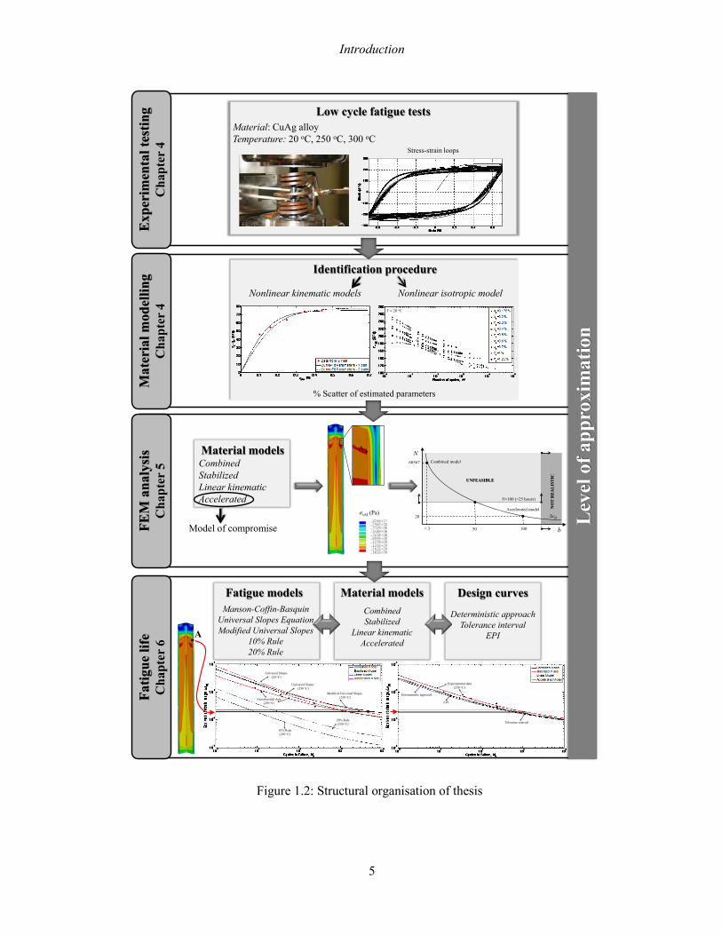
Figure 1.2: Structural organisation of thesis
% Scatter of estimated parameters
Nonlinear kinematic models
Identification procedure
Exp
erim
enta
l tes
ting
Cha
pter
4
Low cycle fatigue testsMaterial: CuAg alloyTemperature: 20 oC, 250 oC, 300 oC
Stress-strain loopsM
ater
ial m
odel
ling
Cha
pter
4 T = 20 oC
Nonlinear isotropic model
FEM
ana
lysi
sC
hapt
er5
σvM (Pa)
A
60567
N
b
Combined model
20
≈ 3 100
Accelerated model
N=100 (≈25 hours)
UNFEASIBLE
Δεpl
NO
T R
EA
LIS
TIC
50
Material modelsCombinedStabilizedLinear kinematicAccelerated
Model of compromise Lev
el o
f app
roxi
mat
ion
Universal Slopes(20 oC)
Experimental data (250 oC)
10% Rule(250 oC)
20% Rule(250 oC)
Universal Slopes(250 oC)
Modified Universal Slopes(250 oC)
Deterministic approach
Experimental data (250 oC)
EPI
Tolerance interval
CombinedStabilized
Linear kinematicAccelerated
Material modelsFatigue modelsManson-Coffin-Basquin
Universal Slopes EquationModified Universal Slopes
10% Rule20% Rule
Design curves
Deterministic approachTolerance interval
EPIA
Fatig
ue li
feC
hapt
er6

Introduction
6
Thesis is organized in seven chapters. Chapter 1 gives the motivation and the aim of this research
work.
Chapter 2 gives an overview of the theoretical background required to understand monotonic and
cyclic loading. Furthermore, some of phenomena which can be observed during cyclic loading are briefly
described. Various simplified material models suitable to describe elasto-plastic deformation in case of
uniaxial monotonic loading are also given.
Chapter 3 describes three main concepts that can be found in the theory of plasticity: the yield
criterion, flow rules and hardening models. Hardening models could be divided in two specified groups,
namely kinematic and isotropic hardening models. Many different hardening models, capable of capturing
elasto-plastic material behaviour under cyclic loadings, have been proposed in the literature [Chaboche,
2008, Lemaitre, 1990]. Some of them are presented and described in this Chapter.
At the beginning of Chapter 4, isothermal low-cycle fatigue (LCF) experimental testing of CuAg alloy
at three temperature levels is described. Furthermore, identification procedure of the nonlinear kinematic
and the nonlinear isotropic material parameters is described. Calibration of the nonlinear kinematic and
the nonlinear isotropic parameters is performed separately, based on isothermal LCF tests of CuAg alloy.
Identification procedure of the material parameters for nonlinear kinematic model can be carried out by
using different approaches. Parameters for the linear kinematic model are estimated considering the tensile
test data. Particular attention, in the last section, is focused on importance of using correct parameters to
obtain qualitative results.
Chapter 5 describes, as a case study, the thermo-mechanical analysis of a copper mould used in the
continuous casting process. The mould is usually made of copper alloys because of their high conductivity
that helps the solidification of the steel. Description of the component and working conditions is given at
the beginning of Chapter 5. The material parameters estimated in Chapter 4 are used as input data for the
structural analysis. The material behaviour response regarding various material models is evaluated as
well. The metallurgical analysis of the copper mould and obtained results are discussed in this Chapter.

Introduction
7
Chapter 6 describes several strain-based fatigue models (Manson-Coffin-Basquin equation, Universal
Slopes equation, Modified Universal Slopes equation, 10% and 20% Rule), which due to their simplicity
and ease of use, are suitable for industrial applications. Particular attention is focused on fatigue models
whose parameters can be estimated using simple tensile test data. Parameters for the Universal Slopes
equation, the Modified Universal Slopes equation are calibrated from experimental tensile tests data. The
Manson-Coffin-Basquin parameters are determined from isothermal LCF test data. Afterwards, several
design curves calculated with the deterministic and probabilistic methods are presented. Correlation
between the material models (combined, stabilized linear and accelerated model) and the fatigue models
(experimental lines, Universal Slopes equation, Modified Universal Slopes equation, 10% Rule and 20%
Rule) as well as comparison between the material models and the design curves are performed.
Concluding remarks of the thesis are given in Chapter 7, which highlight the importance of choosing
an appropriate material model and a fatigue model to accurately assess service life of a component.


Behaviour of materials under monotonic and cyclic loading
9
Chapter 2
Behaviour of materials under monotonic and
cyclic loading
Chapter 2 provides a short overview regarding materials subjected to monotonic and cyclic loading.
Theoretical background of uniaxial monotonic loading is described briefly in order to introduce basic
notation which is going to be used in the thesis. Several phenomena can be observed (e.g. hardening,
softening, combination of hardening and softening and etc.) once a material is subjected to reversed
loading; some phenomena are described in addition. Furthermore, several simplified material models able
to quantitatively describe elasto-plastic deformation in case of monotonic loading are presented at the end
of this Chapter.
2.1 Uniaxial monotonic test
Uniaxial tensile testing is commonly used for measuring mechanical properties of materials. During the
tension test, load is applied to a standard test specimen and causes gradually elongation and eventual
fracture of a specimen. Applied load and an amount of elongation are recorded and plotted on a load-
elongation curve to calculate stresses and strains. Two types of stress-strain curves are possible to
determine based on the load-elongation curve: an engineering stress-strain curve and a true stress-strain
curve [ASTM, ASM, 2000, ASM, 2004, Stephens, 2001]. The engineering stress (σ) is defined as:
0
FA
σ = 2.1
where F is the applied force and A0 is the initial cross-section area.
Behaviour of materials under monotonic and cyclic loading
10
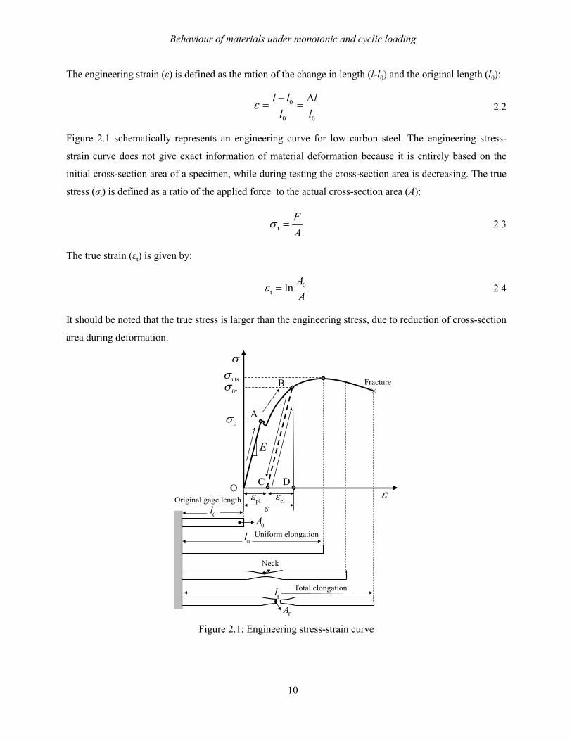
The engineering strain (ε) is defined as the ration of the change in length (l-l0) and the original length (l0):
0
0 0
l l ll l
ε − ∆= = 2.2
Figure 2.1 schematically represents an engineering curve for low carbon steel. The engineering stress-
strain curve does not give exact information of material deformation because it is entirely based on the
initial cross-section area of a specimen, while during testing the cross-section area is decreasing. The true
stress (σt) is defined as a ratio of the applied force to the actual cross-section area (A):
tFA
σ = 2.3
The true strain (εt) is given by:
0
t ln AA
ε = 2.4
It should be noted that the true stress is larger than the engineering stress, due to reduction of cross-section
area during deformation.
Figure 2.1: Engineering stress-strain curve
σ
ε
0σ
E
B
O C
plεε
A
elεD
utsσFracture
0l0A
v ul
Neck
fl
fA
Original gage length
Uniform elongation
Total elongation
0*σ

Behaviour of materials under monotonic and cyclic loading
11
Linear portion of a stress-strain curve up to the initial yield stress (σ0) is known as the elastic region, while
a plastic region is placed beyond σ0. In the elastic region σ < σ0, the stress-strain relation is described by
the Hook’s law:
elEσ ε= ⋅ 2.5
where E is the Young’s modulus, a temperature dependent parameter and εel is the elastic strain. The
specimen starts to deform both plastically and elastically with further increasing a load, exceeding the
initial yield stress and entering in the plastic region. The total strain (ε) is the sum of the elastic and the
plastic strain (εpl) components, as shown in Figure 2.1:
el plε ε ε= +
2.6
The Young’s modulus, the initial yield stress, the ultimate tensile stress (σuts) and the reduction in area
(%RA) are material parameters obtained from the tension test. The percentage of reduction in area is
expressed as:
0 f
0
% 100A ARAA
−= ⋅
2.7
where Af is the area of specimen at fracture. Ductility (D) is degree of the plastic deformation that a
material can undergo before fracture and it can be expressed by:
100ln
100 %D
RA = −
2.8
2.2 Unloading and reloading
Considering a tensile test, see Figure 2.1, in which a specimen is initially loaded in tension until point
B and then unloaded until point C. Both the elastic and the plastic strain occur in the point B. The plastic
strain is permanent strain that remains after unloading, while the elastic strain vanishes after unloading.
When the load is reduced, the strain decreases following the unloading path BC that is parallel to the
initial path OA. Once the load is zero, the total strain is not zero due to amount of the plastic strain which
remains in the point C. Amount of the plastic strain in the point C is equal to the OC line, while the CD
line represents amount of the elastic strain. When the specimen is reloaded, the stress-strain curve follows
the reloading path CB, which is identical with the unloading path BC. The specimen is elastic until the
previous maximum reached stress in the point B. Stress in the point B is regarded as the actual yield stress
(σ0*), beyond which plastic deformation starts to occur again.
Behaviour of materials under monotonic and cyclic loading
12
The stress-strain curve continues to rise although a slope becomes progressively less once the initial yield
stress is reached; thus the actual yield stress increases with further straining. The effect when a material is
able to withstand the greater stress after plastic deformation is known as the strain hardening or the work
hardening [Chen, 1988, Lemaitre, 1990].
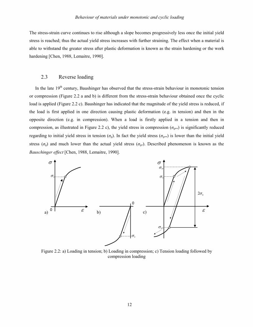
2.3 Reverse loading
In the late 19th century, Baushinger has observed that the stress-strain behaviour in monotonic tension
or compression (Figure 2.2 a and b) is different from the stress-strain behaviour obtained once the cyclic
load is applied (Figure 2.2 c). Baushinger has indicated that the magnitude of the yield stress is reduced, if
the load is first applied in one direction causing plastic deformation (e.g. in tension) and then in the
opposite direction (e.g. in compression). When a load is firstly applied in a tension and then in
compression, as illustrated in Figure 2.2 c), the yield stress in compression (σ0**) is significantly reduced
regarding to initial yield stress in tension (σ0). In fact the yield stress (σ0**) is lower than the initial yield
stress (σ0) and much lower than the actual yield stress (σ0*). Described phenomenon is known as the
Bauschinger effect [Chen, 1988, Lemaitre, 1990].
Figure 2.2: a) Loading in tension; b) Loading in compression; c) Tension loading followed by
compression loading
0σ
σ
ε0
0
0σ
0σ
02σ
0**σ
σ
ε
0*σ
a) b) c)

Behaviour of materials under monotonic and cyclic loading
13
2.4 Cyclic stress-strain behaviour
Assuming a material which is strain cyclically loaded between two fixed limits. Firstly, a material is
strained up to the positive value +εa by the tensile force; then the tensile force is removed and the
compressive force is applied up to the value -εa. Briefly, a material is subjected to alternate strains ± εa
indefinitely number of times. Figure 2.3 shows a stress-strain loop obtained after first cycle. The stress-
strain loop is characterized by the total strain range (Δε) and the stress range (Δσ).
Figure 2.3: Stress-strain hysteresis loop
The total strain range can be decomposed into the elastic range (Δεel) and the plastic strain range (Δεpl)
components [Chen, 1988, Lemaitre, 1990]:
el plε ε ε∆ = ∆ + ∆ 2.9
The elastic strain range is related to the stress range (Δσ ≡ σmax-σmin) by:
el Eσε ∆
∆ =
2.10
Let
plel
a el,a pl,a; ; 2 2 2
εε εε ε ε∆∆ ∆
≡ ≡ ≡
plε∆ elε∆ε∆
σ∆
σ
ε

Behaviour of materials under monotonic and cyclic loading
14
define the strain amplitude (εa), the elastic strain amplitude (εel,a) and the plastic strain amplitude (εpl,a),
respectively. With the stress amplitude (σa ≡ Δσ/2), additional decomposition of the strain amplitude can
be rewritten as:
a
a pl,aEσε ε= +
2.11
Material stress-strain response is affected by cyclic loading. A stress required to achieve straining, as
shown in Figure 2.3, do not remain constant but change as cycling proceeds. The manner in which stress
vary depends on type of a material and can be classify into three different categories: hardening, softening
and combination of hardening and softening.
2.5 Effect of cyclic loading: hardening and softening
For strain controlled loading, the hardening is said to occur when the stress range progressively
increases to maintain the same strain range as cycling proceeds, see Figure 2.4 a. The stress range settles
down to an aproximately constant value after certain number of cycles. Value at which the stress settles
down is known as the saturated stress range and depends on the imposed strain range. The saturated stress
range is reached often within 10% to 40% of the total life. Since, the stress range is rather constant over a
large part of live; the stabilized cycle is defined as the cycle that corresponds to the mid-life of the
specimen, i.e. equal to the half number of cycles required to failure. In case of stress controlled loading,
the hardening is said to occur when the strain range progressively decreases to maintain the same stress
range as the cycling proceeds as can be seen in Figure 2.4 b, or when the stress range increases in a stress
controlled test, see Figure 2.4 a. On the other hand, the softening is said to occure when the stress range
decreases with successive cycles under controlled strain (Figure 2.4 c), or when the strain range increases
in a stress controlled test, see Figure 2.4 d. [Coffin, 1972, Lemaitre, 1990, Manson, 1965, Manson, 1966,
Stephens, 2001]
Hardening and/or softening phenomena are more pronounced at the beginning of cyclic loading. Some
materials like copper, stainless steels show significant softening/hardening, while other materials (e.g.
structural steel) do not show so obviously this phenomenon. Furthermore, some materials harden at the
beginning of cyclic loading and after certain number of cycles start to soften. Properties of cyclic
hardening or softening do not depend only on material microstructure, temperature, but also on loading
amplitude or more generally on previous strain history. Both phenomena are believed to be associated
with stability of the dislocation substructure within the metal crystal lattice of a material [Halama, 2012,
Lemaitre, 1990].

Behaviour of materials under monotonic and cyclic loading
15
Controlled strain Controlled stress H
arde
ning
a) b)
Softe
ning
c) d)
Figure 2.4: Phenomena of cyclic hardening and softening
Manson observed that the ration of monotonic ultimate strenght (σuts) to the 0.2% offset yield strenght (σ0)
can be used to predict whether the material will soften or harden. If σuts/ σ0 >1.4, a material is likely to
cyclically strain harden; while a material is likely to soften if σuts/ σ0<1.2 [Manson, 2006].
2.6 Simplified uniaxial monotonic stress-strain curves
Several simplified models have been proposed in literature to describe quantitatively the elasto-plastic
deformation of materials. Some of them are presented and described in the following paragraphs.
2.6.1 Elastic-perfectly plastic model
The elastic-perfectly plastic model assumes a null strain-hardening effect, i.e. the plastic deformation
occurs as the stress reaches the yield stress. As can be seen in Figure 2.5, the uniaxial stress-strain diagram

Behaviour of materials under monotonic and cyclic loading
16
beyond the yield stress is approximated by a horizontal straight line with a constant stress level σ0. The
relation for the elastic-perfectly plastic model can be expressed as [Chen, 1988]:
0
0
for
for Eσε σ σ
ε σ σ
= < = ∞ =
2.12
Using elasto-perfectly plastic model can lead to drastic simplification of an analysis. However, in some
applications (e.g. for studying processes where material is worked at a high temperature –such as hot
rolling) are allowed and suitable to neglect the effect of strain hardening
2.6.2 Elastic-linear strain hardening model
The elastic-linear strain hardening model supposes that the continuous curve is approximated with two
straight lines. As can be seen in Figure 2.6, the first line has a slope of Young’s modulus, while the second
straight line presents an idealization for the strain hardening range and has a slope which corresponds to
the tangent modulus (Et), where Et < E. The stress-strain relation is expressed by [Chen, 1988]:
( )
0
00 0
t
for
1 for
E
E E
σε σ σ
σε σ σ σ σ
= ≤ = + − >
2.13
Figure 2.5: Elastic-perfectly plastic model Figure 2.6: Elastic-linear strain hardening model
σ
ε
E
0σ
σ
ε
tE
E
0σ
Behaviour of materials under monotonic and cyclic loading
17
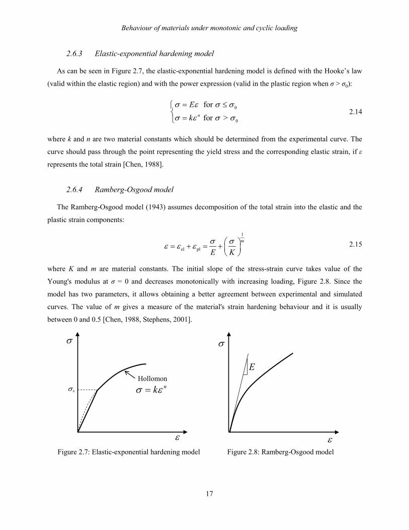
2.6.3 Elastic-exponential hardening model
As can be seen in Figure 2.7, the elastic-exponential hardening model is defined with the Hooke’s law
(valid within the elastic region) and with the power expression (valid in the plastic region when σ > σ0):
0
0
for
for > n
Ek
σ ε σ σ
σ ε σ σ
= ≤
= 2.14
where k and n are two material constants which should be determined from the experimental curve. The
curve should pass through the point representing the yield stress and the corresponding elastic strain, if ε
represents the total strain [Chen, 1988].
2.6.4 Ramberg-Osgood model
The Ramberg-Osgood model (1943) assumes decomposition of the total strain into the elastic and the
plastic strain components:
1
el pl
m
E Kσ σε ε ε = + = +
2.15
where K and m are material constants. The initial slope of the stress-strain curve takes value of the
Young's modulus at σ = 0 and decreases monotonically with increasing loading, Figure 2.8. Since the
model has two parameters, it allows obtaining a better agreement between experimental and simulated
curves. The value of m gives a measure of the material's strain hardening behaviour and it is usually
between 0 and 0.5 [Chen, 1988, Stephens, 2001].
Figure 2.7: Elastic-exponential hardening model Figure 2.8: Ramberg-Osgood model
σ
ε
nkσ ε=Hollomon
0σ
σ
ε
E

Behaviour of materials under monotonic and cyclic loading
18
Chapter 2 gives briefly theoretical overview of several topics (uniaxial monotonic loading, cyclic
loading, hardening and softening phenomena, and etc ). Discussed topics are theoretical base of the work
presented in the following sections. Notation used thought the thesis is also defined in this Chapter.
Several simplified models (elastic-perfectly plastic, the elastic-linear strain hardening, the elastic-
exponential hardening and Ramberg-Osgood model), suitable to quantitatively describe the plastic
deformation for the monotonic case of loading, are presented. Following Chapter 3 presents models that
can be used for both monotonic and cyclic loading cases as well as gives overview of three main concepts
which can be found in the theory of plasticity.
Theoretical plasticity models
19
Chapter 3
Theoretical plasticity models
Chapter 3 gives an overview of three main concepts which can be found in the theory of plasticity: the
yield criterion, the flow rule and hardening models. The yield criterion is needed to define the limit of
elasticity, i.e. the limit at which material becomes plastic. The flow rule describes the relationship between
an applied stress increment and a resulting plastic strain increment once a material has become plastic. In
addition, the rule defines magnitude and direction of the plastic flow. Hardening models take into
consideration evolution of the yield surface by describing the change in the yield criterion as a function of
plastic strain. The subsequent yield stress, of a material subjected to reversed loading, is usually
determined by one of two models: kinematic and/or isotropic models. Several material models have been
developed and described in the literature over the years. However, only few kinematic and isotropic
models are theoretically presented in this Chapter.
Numerical simulations are performed considering the simple numerical model and adopting several
material models. The goal of performed activities is to get an overview and a link between theoretical and
practical use of material models. In addition, sensitivity analyses are done in order to understand better
which parameters do really affect and how on a material response. Obtained results are described and
presented in the second part of Chapter 3.

Theoretical plasticity models
20
3.1 Stress deviator tensor and plastic strain increment tensor
In material modelling, the stress tensor (σ) is convenient to split into two parts the hydrostatic stress
tensor (σH) and the stress deviator tensor (σ'). The stress tensor can be written [Chen, 1988, Lemaitre,
1990]:
11 12 13 H 11 H 12 13
21 22 23 H 21 22 H 23
31 32 33 H 31 32 33 H
0 00 00 0
σ σ σ σ σ σ σ σσ σ σ σ σ σ σ σσ σ σ σ σ σ σ σ
− = = + −
−
σ
3.1
The hydrostatic stress is an average of the three stress components:
( )H 1 2 313
σ σ σ σ= + +
3.2
where σ1, σ2, σ3 are principal stresses in 1, 2, and 3 direction, respectively. The hydrostatic stress tensor is
given by:
H
H H H
H
0 00 00 0
σσ σ
σ
=
σ I = 3.3
where I is the unit tensor. The stress deviator tensor is obtained by subtracting the hydrostatic stress tensor
from the stress tensor:
11 H 12 13
H 21 22 H 23
31 32 33 H
-´ -
-
σ σ σ σσ σ σ σσ σ σ σ
= − =
σ σ σ 3.4
The plastic strain rate tensor (dεpl) can be expressed as:
pl,11 pl,12 pl,13
pl pl,21 pl,22 pl,23
pl,31 pl,32 pl,33
d d dd d d d
d d d
ε ε εε ε εε ε ε
=
ε 3.5
The accumulated plastic strain increment (dεpl,acc) is defined as [Chaboche, 2008, Lemaitre, 1990]:
plplpl,acc d:d32d εε=ε 3.6
where the symbol ‘:’ is called the double contracted product, or double dot product, of two second order
tensors (e.g. A and B). Multiply component by component and sum the terms gives a scalar quantity:
1 1
:n n
ij iji j
A B A B= =
= ∑∑ 3.7

Theoretical plasticity models
21
3.2 Yield criterion
The limit of elasticity in uniaxial state of stress is defined by the yield stress. However, exact value at
which material starts to plastically deform is not so trivial to give when several stress components are
present and act simultaneously. The yield criterion defines the limit of elasticity of a material under
combined state of stress and mathematically can be expressed as [Besson, 2010, Dunne, 2005, Lemaitre,
1990, Stephens, 2001]:
( ) 0f =σ 3.8
For isotropic materials, the yield function can be visualized as a yield surface in three dimensional stress
space in which each of coordinate axes represents the one principal stress. The yield surface divides the
stress space into the elastic and the plastic regions; the elastic deformation occurs when f (σ) < 0, while the
plastic deformation occurs when f (σ) = 0. Several criterions can be found in literatures to describe the
yield surface [Besson, 2010]. Only the von Mises yield criterion is considered here.
The von Mises is commonly used yield criterion for ductile materials [Besson, 2010, Dunne, 2005,
Lemaitre, 1990, Stephens, 2001]:
( ) 0:23
00vM =−=−= σσσ σ'σ'σf 3.9
where σvM is the von Mises stress. The von Mises stress can be expressed in terms of principal stresses as:
( ) ( ) ( )2132
322
21vM 21 σσσσσσσ −+−+−= 3.10
As can be seen in Figure 3.1, the von Mises criterion is visualized as a circular cylinder that is orthogonal
to a deviatoric plane in the stress space and parallel to the hydrostatic axis σ1 = σ2 = σ3. The criterion
becomes an ellipse considering the plane state of stress (σ3 = 0) as can be seen in Figure 3.2 [Besson,
2010, Dunne, 2005].
Figure 3.1: The von Mises yield surface
1σ2σ
3σ
1 2 3σ σ σ= =
Hydrostatic axis
1 2 3 0σ σ σ+ + =
Deviatoric plane
von Mises yield surface
2σ
3σ
1σ
Yield surface
Elastic region

Theoretical plasticity models
22
3.3 Flow rules
The flow rule relates stresses and plastic strains once the plastic deformation has begun. Equations
which relate stress increments and plastic stains increments are called constitutive equations and are
typically based on the normality condition. The normality condition states that the increment of a plastic
strain caused by an increment of stress is such that the vector representing the plastic strain increment is
normal to the yield surface during the plastic deformation [Stephens, 2001].
In 1928, von Mises proposed the concept of the plastic potential function (g), which is a scalar function of
the stresses. The plastic flow equation, based on the plastic potential function, can be written in the form
[Chen, 1988, Lee, 2012, Lemaitre, 1990]:
σ
ε∂∂
=gλdd pl 3.11
where dλ is a positive scalar of proportionality, which is nonzero only when the plastic deformation occur.
Several flow rules have been proposed in the literature over the years, however, only the associated flow
rule is considered and explained in addition.
The associated flow rule assumes that the plastic potential function and the yield function coincide (g = f ).
Based on this assumption, equation (3.11) is possible to rewrite as [Chen, 1988, Lee, 2012]:
pld d fλ ∂=
∂ε
σ 3.12
Direction of the plastic strain increment is given with ∂f/∂σ and it is a vector normal to surface. The strain
increment can be plotted as a vector normal to the surface with a length determined by dλ, as shown in
Figure 3.2.
Figure 3.2: Associated flow rule with von Mises yield condition for plane stress
2σ
1σ
0σ
0σ
0σ 0σStress point
Elastic regionYield surface ( )0f =
Tangent to yield surface
2pl,dεpldε
1pl,dε

Theoretical plasticity models
23
3.4 Loading surface
The subsequent yield surface for an elasto-plastically deformed material is called the loading surface.
Three different conditions are possible to occur when a stress point is considered to be on the surface:
unloading, neutral loading and loading, see Figure 3.3. The plastic deformation will not occur when the
stress point is considered to be within loading surface. On the other hand, the additional plastic
deformation occurs if the stress point is on the surface and tends to move out of the current loading
surface, simultaneously causing change of the current loading surface. The loading surface can change
size, shape, position and be described as [Chen, 1988, Lemaitre, 1990]:
( ), 0f κ =σ 3.13
where κ represents one or more hardening parameter (parameter may be scalar or higher order tensor),
which changes during the plastic deformation and defines evolution of the yield surface. The hardening
parameters are zero when material starts to deform plastically for a first time:
( ) ( )0,0f f=σ σ 3.14
a) Multiaxial case b) Uniaxial case
Figure 3.3: Loading criterion for a strain hardening material
One of major problems in the strain hardening theory is to determine nature of the subsequent loading
surface. Response of a material after initial yielding mainly depends on a considered plasticity model.
3.5 Hardening models
Many hardening models have been developed and described in literatures until now. Some of them can
be found in [Chaboche, 1983a, Chaboche, 1983b, Chaboche, 1986a, Chaboche, 1986b, Chaboche, 1989,
Chaboche, 2008, Lemaitre, 1990]. Hardening models describe change in the yield criterion as a function
of the plastic strain. Generally, the hardening phenomenon is described with one of two specific types:
Loading surface
1σ
2σ Neutral loading
Loading Unloading
σ
ε
Stress point
Loading
Unloading

Theoretical plasticity models
24
namely kinematic and isotropic hardening. The kinematic and the isotropic hardening are described in this
section.
3.5.1 Kinematic hardening material models
Kinematic hardening material models assume translation of the loading surface as a rigid body in the
stress space simultaneously maintaining size, shape and orientation of the initial yield surface. The
kinematic hardening captures the Bauschinger effect as a consequence of an assumption that the loading
surface translates as a rigid body (i.e. the elastic range is assumed to be unchanged during hardening)
[Chen, 1988, Silvestre, 2015]. Considering the von Mises criterion, the yield function is convenient to
write as [Dunne, 2005, Chaboche, 1986a, Lemaitre, 1990]:
( ) ( ) ( ) 0:23, 0 =−′−′′−′= σκ ασασσf 3.15
The back stress, α, indicates present position of the loading surface (i.e. centre of the loading surface),
which may be shifted as a result of the kinematic hardening mechanism; while α´ is the deviatoric part of
α. The back stress has the same components as the stress; therefore, it can be written as tensor and
considered as a deviator because of the plastic incompressibility [Lemaitre, 1990].
3.5.1.1 Linear kinematic hardening – Prager’s model
Prager (1949) proposed the linear kinematic hardening model which assumes collinear relation
between increment of the kinematic variable (dα) and the plastic strain increment [Chaboche, 1986a,
Chaboche, 2008, Dunne, 2005, Lemaitre, 1990]:
pl2d d3
C=α ε 3.16
The initial hardening modulus, C, is temperature dependent material parameter. The yield surface, under
applied load which causes the plastic deformation, translates to a new location. The initial centre is
translated by α.
The Prager’s model is schematically illustrated in Figure 3.4. Imagine a specimen which is firstly loaded
up to the point B and then until the point B’. Both the elastic and the plastic deformations occur in the
point B while only the elastic deformation appears between the points B and B’. However, the elasto-
plastic deformation occurs again when an applied load pass the point B’. Radius of the yield surface is
equal to the initial yield stress confirming that the linear kinematic hardening model is able to capture the
Bauschinger effect. The main advantage of this model is having only one material parameter, C.

Theoretical plasticity models
25
a) Stress space b) Tension-compression
Figure 3.4: Evolution of the linear kinematic hardening model
As can be seen in Figure 3.4, the negative aspect of the Prager’s model is that transition from the elastic to
the plastic region is not smooth; i.e. it is described with a sharp angle which connects two straight lines. It
would be much better that transition is defined with a continuous curve in order to get more realistic
curve.
3.5.1.2 Nonlinear kinematic hardening –Armstrong and Frederick’s model
Armstrong and Frederick (1966) proposed more complex nonlinear kinematic hardening model to
obtain smoother transition from the elastic to the plastic region. Proportionality between dεpl and dα is
eliminated by adding, on the Prager’s model, a recall term which introduces a fading memory effect to the
strain path [Chaboche, 1986a, Chaboche, 2008, Lemaitre, 1990]:
pl pl,acc2d d d3
C γ ε= −α ε α 3.17
The nonlinear recovery parameter, γ, is temperature dependent material parameter while dεpl,acc is the
increment of the accumulated plastic strain. The recall term affects to the plastic flow differently for
tensile or compressive loading because it depends on |dεpl| and it is important in predicting a nonlinear
stress-strain loop under cyclic loading [Khan, 1995]. The nonlinear recovery parameter controls the rate at
which the initial hardening modulus decreases with increasing the plastic strain. Moreover, γ determines
the rate of stress saturation. Evolution of the back stress instead of being linear is now exponential for
monotonic uniaxial loading.
Initial yield surface ( f0= 0 )
Subsequent yield surface ( f = 0 )
O
A B
B’
maxσ0σ
0σ
1σ
2σ 3σ
ε
σ
α0σ
O
σ
plε
maxσ0σ
0σ
αC

Theoretical plasticity models
26
a) Stress space b) Tension-compression
Figure 3.5: Evolution of the nonlinear kinematic hardening model
Considering a component that has been loaded following the loading path O-A-B-B’, see Figure 3.5, a
material starts to elasto-plastic deform after passing the initial yield stress (the point A). In this case, the
transition from the elastic to the plastic region is smooth. The back stress increases with the increasing the
plastic strain and saturates to the value C/γ; giving the maximum saturated stress equal to σ0+ C/γ. Shape
of the stress-strain curve, obtained using the nonlinear kinematic hardening model, is more similar to the
form of experimental stress-strain curves. For uniaxial case of loading, where σ = σ11 ≠ 0 and σ22= σ33= 0,
von Mises criterion (equation 3.15) can be written as [Chaboche, 1986a, Lemaitre, 1990]:
0 0f σ α σ= − − = 3.18
Considering assumption of the plastic incompressibility, dεpl = dεpl,11 ≠ 0, dεpl,22 = dεpl,33 = -1/2 dεpl, gives
the accumulated plastic strain equal to:
pl,acc pl pl pl2d d : d d3
ε ε= =ε ε 3.19
The nonlinear hardening model (expressed with equation 3.17) may be written as:
pl pld d dα C ε α εγ= − 3.20
Essential difference between two plastic strain increment terms dεpl and dεpl,acc is that they give rise to dεpl
and |dεpl|, respectively. Thus, nonlinearity introduced by the recall term is not the same during the flow
under the tensile or the compressive loading. Relation between α and εpl is no unique and the concavity of
the stress-strain curve is correctly reproduced [Chaboche, 1986a]. For tension-compression, the absolute
Initial yield surface( f0= 0 )
Subsequent yield surface( f = 0 )
O
AB
B’
maxσ0σ
1σ
2σ 3σ
ε
σ
O
σ
plεα α
maxσ0σ
0σ
C
C γ
0σ
0σ
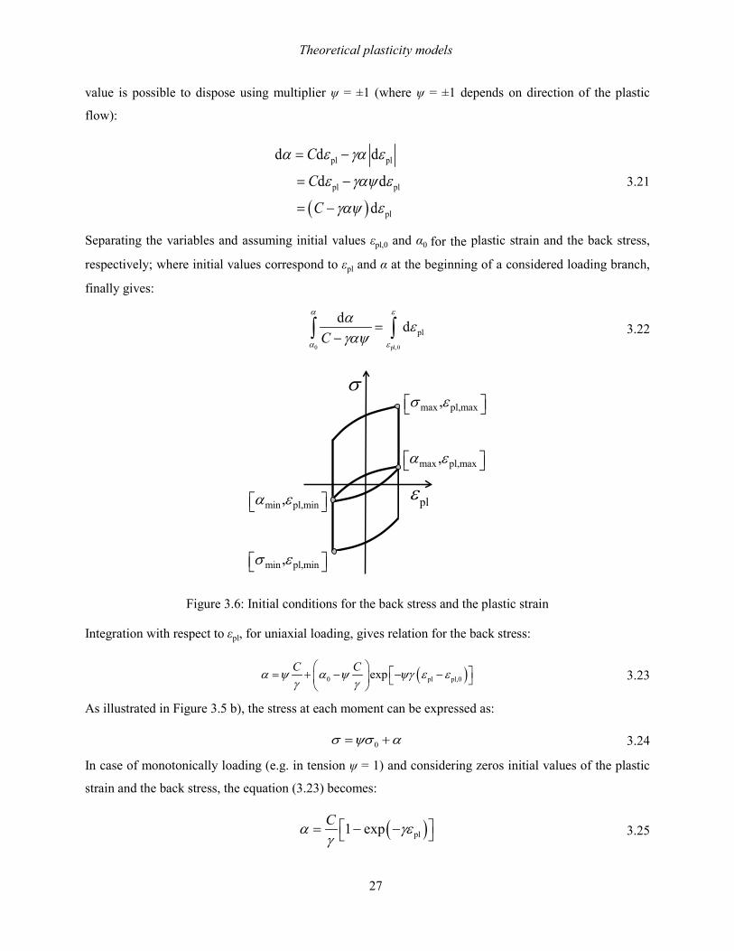
Theoretical plasticity models
27
value is possible to dispose using multiplier ψ = ±1 (where ψ = ±1 depends on direction of the plastic
flow):
( )
pl pl
pl pl
pl
d d d
d d
d
C
C
C
α ε γα ε
ε γαψ ε
γαψ ε
= −
= −
= −
3.21
Separating the variables and assuming initial values εpl,0 and α0 for the plastic strain and the back stress,
respectively; where initial values correspond to εpl and α at the beginning of a considered loading branch,
finally gives:
0 pl,0
pld d
C
α ε
α ε
α εγαψ
=−∫ ∫
3.22
Figure 3.6: Initial conditions for the back stress and the plastic strain
Integration with respect to εpl, for uniaxial loading, gives relation for the back stress:
( )0 pl pl,0expC Cα ψ α ψ ψγ ε εγ γ
= + − − − 3.23
As illustrated in Figure 3.5 b), the stress at each moment can be expressed as:
0σ ψσ α= + 3.24
In case of monotonically loading (e.g. in tension ψ = 1) and considering zeros initial values of the plastic
strain and the back stress, the equation (3.23) becomes:
( )pl1 expCα γεγ = − −
3.25
σ
plε
max pl,max,σ ε
min pl,min,σ ε
min pl,min,α ε
max pl,max,α ε

Theoretical plasticity models
28
Equation (3.25) is proposed to use for identification of material parameters C and γ using a single
stabilized stress-strain loop [Chaboche, 1986a, Chaboche, 2008, Lemaitre, 1990]. Limit values of the
parameters (C and γ) show the influence on stress-strain response of the nonlinear kinematic hardening
model:
( )pl
pl0lim expC Cε
γε→
− =
3.26
( )
pl0 pl 0lim 1 expC C
εσ γε σ
γ γ→∞ + − − = +
3.27
The back stress, α, saturates to C/γ for sufficiently large (εpl - εpl,0) [Hu, 1999]. Maximum (σmax, εmax) and
minimum (σmin, εmin) values are constant in the stabilized cycle. The plastic strain at end of the loading
branch is an initial value of the unloading branch. The maximum back stress, in case of tension (ψ = 1),
can be expressed using equation (3.23) as:
( )max min pl,max pl,minexpC Cα α γ ε εγ γ
= + − − − 3.28
where εpl,max is the maximum plastic strain and εpl,min is the minimum plastic strain. Similarly, the minimum
back stress, for compression (ψ = -1), is expressed as:
( )min max pl,min pl,maxexpC Cα α γ ε εγ γ
= − + + − 3.29
Specifying the plastic strain range as Δε= εmax - εmin, the stress range Δσ= σmax - σmin and using fact that:
max max 0*σ α σ= + 3.30
min min 0*σ α σ= − 3.31
Relation between the half stress range and the half strain range under stabilized cycling can be obtained by
substituting equation (3.28) to (3.29):
∆+=
∆2
tanh2
pl0
εγ
γσσ C
3.32
Stabilization in the nonlinear kinematic model occurs only if the loading is symmetrical (zero mean
stress). Quantitatively, the model describes the ratchet effect under nonzero mean stress [Chaboche,
1986a].

Theoretical plasticity models
29
3.5.1.3 Nonlinear kinematic hardening – Chaboche’s model
The nonlinear kinematic hardening model proposed by Chaboche is obtained by superimposing two or
more nonlinear kinematic hardening models proposed by Armstrong & Frederick [Chaboche, 1986a,
Chaboche, 1989, Chaboche, 2008, Lemaitre, 1990]:
m
ii
= ∑α α 3.33
Each of the kinematic variables αi works independently:
pl pl,acc2d d d3i i i iC γ ε= −εα α 3.34
The range of validity is widened using the Chaboche’s model. Three kinematic variables (m = 3) are
sufficient to cover strain ranges between 0.01% and 4% [Chaboche, 1986a]. Superposition of several
Armstrong & Frederick’ models are able to describe more accurate three critical segments of a stable
hysteresis curve:
1) initial modulus when yielding starts to occur,
2) nonlinear transition of the hysteresis curve after yielding starts until the curve becomes linear
again and
3) linear segment of the curve in the range of higher strain.
In the form of Chaboche model, equation (3.32) may be written as [Halama, 2012, Lemaitre, 1990]:
∑
∆+=
∆ m
ii
i
iC2
tanh2
pl0
εγ
γσσ
3.35
3.5.2 Isotropic hardening material models
The isotropic hardening material models assume symmetrically enlargement of the yield surface under
the plastic deformation without changing its centre or shape. Moreover, isotropic hardening models are
able to capture cyclic hardening and/or softening behaviour of a material. An amount of the yield surface
expansion is taken to be a function of the accumulated plastic strain, i.e. the accumulated plastic strain is
assumed to be the hardening parameter (εpl,acc = κ). Considering the von Mises criterion, the yield function
is convenient to write as [Dunne, 2005, Chaboche, 1986a, Chaboche, 2008, Lemaitre, 1990]:
( ) ( )0* pl,acc3, : 02
f κ σ ε′ ′= − =σ σ σ 3.36
where σ0*(εpl,acc) is the actual yield stress and might have a form:

Theoretical plasticity models
30
( ) ( )0* pl,acc 0 pl,accRσ ε σ ε= + 3.37
where R(εpl,acc) is the isotropic hardening function. Many isotropic hardening models have been developed
until now. In addition some of models are presented and described.
3.5.2.1 Linear isotropic hardening model
The linear isotropic hardening material model assumes that the evolution of the loading surface is
governed only by one scalar variable (εpl,acc). To simplify the presentation, the rule is developed assuming
constant temperature or at least using criteria which are temperature independent [Dunne, 2005, Lemaitre,
1990]:
pl,acc( )R R ε= 3.38
in which R is the drag stress and describes size of the yield surface. Figure 3.7 schematically shows the
isotropic hardening model in terms of the von Mises criterion. In case that applied load in the point B
continues to increase in tension until the point M or if in the point B is applied a load in compression until
the point M’, an amount of the accumulated plastic strain is the same in both cases due to OI+IP=OI+IP’.
As can be noticed in Figure 3.7, the isotropic hardening is able to capture uniquely enlargement of yield
surface in all direction. Value of the actual yield stress in tension σ0* = σB is equal to the actual yield stress
in compression σB’. Consequently, the isotropic hardening model neglects completely the Bauschinger
effect.
a) Stress space b) Tension-compression
Figure 3.7: Evolution of the linear isotropic hardening model
Initial yield surface( f0= 0 )
Subsequent yield surface( f = 0 )
O
AB
C
B’
0σ0*σ
0*2σ
σ
ε
2σ 3σ
1σ
O
M
I PP’
σ
plε
M’
0*σ0σ
B

Theoretical plasticity models
31
3.5.2.2 Nonlinear isotropic hardening model
The evolution of the yield surface size may be expressed with the nonlinear isotropic hardening model
[Chaboche, 1989, Chaboche, 2008, Lemaitre, 1990]:
( ) ( )pl,acc pl,accd dR b R Rε ε∞= − 3.39
where b indicates the speed of stabilization and R∞ is the saturated stress (maximum increment) of R. Both
material parameters are temperature dependent. The achieved peak of the stress is equal to (σ0+R∞),
obtained from equation (3.37). The relation between R and εpl,acc is obtained after integration:
( )pl,acc1 expR R bε∞ = − − 3.40
R∞ can be either positive or negative, giving rise to cyclic hardening or softening, respectively. Moreover,
R stabilizes after certain number of cycles to the value of R∞. The saturated stress is in fact difference
between the maximum stress of the first cycle (σmax,1) and the stabilized one (σmax,s). The application of the
given criterion to each uniaxial cycle gives:
( )max 0 pl,acc1 expR bσ σ ε∞ = + − − 3.41
Assuming Δεpl to be approximately constant, the accumulated plastic strain can be written as:
pl,acc pl2 Nε ε= ∆ 3.42
in which N is the number of cycle. Finally is obtained relation which is proposed by [Lemaitre, 1990] to
identify the speed of stabilization:
( ) ( )NbbRRi
placcpl,1max,smax,
1max,max, 2exp1exp1 εεσσσσ
∆−−=−−=≈−−
∞
3.43
where σmax,i is the current maximum stress for the Nth cycle.
a) Stress space b) Tension-compression
Figure 3.8: Evolution of the nonlinear isotropic hardening model
Initial yield surface ( f0= 0 )
Subsequent, expanded yield surfaces after plastic deformation
( f = 0 )
0σ
σ
ε
2σ 3σ
1σ
0σ
R0*σ
R∞
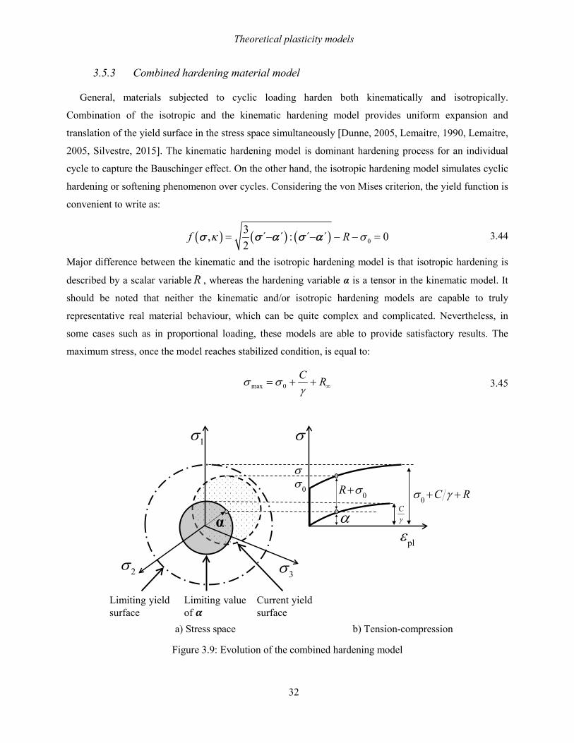
Theoretical plasticity models
32
3.5.3 Combined hardening material model
General, materials subjected to cyclic loading harden both kinematically and isotropically.
Combination of the isotropic and the kinematic hardening model provides uniform expansion and
translation of the yield surface in the stress space simultaneously [Dunne, 2005, Lemaitre, 1990, Lemaitre,
2005, Silvestre, 2015]. The kinematic hardening model is dominant hardening process for an individual
cycle to capture the Bauschinger effect. On the other hand, the isotropic hardening model simulates cyclic
hardening or softening phenomenon over cycles. Considering the von Mises criterion, the yield function is
convenient to write as:
( ) ( ) ( ) 03, ´ ´ : ´ ´ 02
f Rκ σ= − − − − =σ σ α σ α 3.44
Major difference between the kinematic and the isotropic hardening model is that isotropic hardening is
described by a scalar variable R , whereas the hardening variable α is a tensor in the kinematic model. It
should be noted that neither the kinematic and/or isotropic hardening models are capable to truly
representative real material behaviour, which can be quite complex and complicated. Nevertheless, in
some cases such as in proportional loading, these models are able to provide satisfactory results. The
maximum stress, once the model reaches stabilized condition, is equal to:
∞++= RCγ
σσ 0max 3.45
a) Stress space b) Tension-compression
Figure 3.9: Evolution of the combined hardening model
Limiting yield surface
Current yield surface
Limiting value of
1σ
2σ 3σ
σ
σ
0R σ+Cγα
plε
0 C Rσ γ+ +
α
0σ

Theoretical plasticity models
33
3.5.4 Accelerated material model
The accelerated material model, proposed by [Chaboche, 1986a] is in fact the combined model which
takes into consideration the speed of stabilization, b. Therefore, the model is able to capture the monotonic
hardening associated with the cyclic hardening or softening phenomenon. However, with this model is
possible to control the speed of stabilization by increasing or decreasing the coefficient b. The number of
cycles needed to reach the stabilized condition is smaller by imposing the higher value of the b parameter.
3.5.5 Stabilized material model
The stabilized material model, proposed by [Chaboche, 1986a], assumes condition of a material when
it reaches the stabilization (i.e. when R reaches R∞), simultaneously neglecting cyclic hardening or
softening phenomenon. In other words, the stabilized model is almost equal to the nonlinear kinematic
model. Parameters (C and γ) are identical to those described in paragraphs 3.5.1.2 and 3.5.1.3. However,
the main difference between these two models is that the stabilized model neglects the initial state of a
material and takes into consideration the Young’s modulus (Es) and the actual yield stress (σ0*) calculated
from stabilized experimental stress-strain curves. Instead, the kinematic model takes into consideration
initial state of a material, i.e. the initial Young’s modulus (E1) and the initial yield stress (σ0). Differences
between initial values of E1, σ0 and stabilized values Es, σ0* are described more in details in the paragraphs
4.2.1 and 4.2.2.
3.6 Numerical simulations and sensitivity analyses with respect to material
models
So far, several material models (the kinematic, the isotropic and the combined) have been theoretically
presented. The kinematic and the isotropic material models have been already implemented in commercial
FEM codes to provide accurate prediction of material behaviour and different phenomenon such as the
Bauschinger effect, cyclic hardening or softening and etc. The aim of this paragraph is to get a link
between theoretical part and practical use of material models.
The numerical simulations and the sensitivity analyses are done in order to understand better difference
between several material models (the nonlinear kinematic, the nonlinear isotopic and the combined
material model). Similar numerical simulations have been done in [Lee, 2009]. Moreover, sensitivity
analyses are performed to comprehend clearer which parameters do really affect and how on the material
response.

Theoretical plasticity models
34
A simple numerical model, shown in Figure 3.10, is created and used to simulate cyclic loading. The
numerical model is constrained at the bottom and at the top is imposed fully reversed triangular waveform
of displacement (Δl= ±1 mm) as indicated in Figure 3.11. Figure 3.11 shows also the finite element mesh
with boundary conditions.
Figure 3.10: Model used in numerical simulation Figure 3.11: Strain imposed on a model
In this way, proportional strain controlled loading is simulated with the strain amplitude equal to:
a 0,5%ll
ε ∆= = 3.46
where l is the length of the model. Two dimensional 8 node elements are used to create the finite element
model (PLANE183 in ANSYS®). Each simulation demonstrates 20 cycles or 40 load steps. The material
parameters used in simulations are taken from [You, 2008] and presented in Table 3.1. Data for stress-
strain curves are taken in a node at the top in the centre of the model, far from constraints.
Table 3.1: Material parameters
Nonlinear kinematic model Nonlinear isotropic model
E (GPa) σ0 (MPa) ν C (MPa) γ R∞ (MPa) b
125 100 0.36 64257 888 76 8
Imposed axial displacement
Imposed constraints
Δl = ±1 mm
l = 2
00 m
m
h =50 mm
Δl
Load step
1
-1
1 2 3 4

Theoretical plasticity models
35
3.6.1 Nonlinear kinematic hardening – Armstrong & Frederick’s model
The numerical simulation is performed using the numerical model described in Figure 3.10 and
adopting the Armstrong and Frederick’s model.
The Chaboche model has been already implemented in the Ansys® code as a given option inside
structural – nonlinear – inelastic – rate independent section. The Ansys® has a possibility to superimpose
up to five the Armstrong and Frederick’s models simultaneously taking into consideration temperature
dependence or independence of material parameters. In this case, the Armstrong and Frederick’s model is
defined by imposing only the one pair of C, γ and assuming temperature independence of material
parameters.
Resulting stress-strain loops obtained from the numerical simulation are illustrated in Figure 3.12. As can
be seen in Figure 3.12, the model starts to plastically deform once it passes the yield stress (σ0=100 MPa).
Firthermore, the model stabilizes after first cycle confirming the statement of [Chaboche, 1986] in which
it states that the stabilization occurs very fast in case of symmetrical loading with zero mean stress.
According to equation 3.32, the maximum stress when model reaches the stabilization is equal to:
max 0 172 MPaCσ σγ
= + = 3.47
Figure 3.12: Armstrong & Frederick’s material model - stress-strain curves
As can be seen in Figure 3.13, the Armstrong and Frederick’s model is able to capture the Bauschinger
effect and monotonic hardening. However, the model is unable to simulate cyclic hardening/softening,
according to theory presented in paragraph 3.5.1.2.
-0.5 -0.4 -0.3 -0.2 -0.1 0 0.1 0.2 0.3 0.4 0.5-200
-150
-100
-50
0
50
100
150
200
Strain (%)
Stre
ss (M
Pa)

Theoretical plasticity models
36
Figure 3.13: Armstrong & Frederick’s material model – stress vs. load steps
Sensitivity analysis of nonlinear kinematic hardening material parameters - C, γ
The aim of sensitivity analysis is to investigate how C and γ define shape of stress-strain loops. Firstly,
the value of initial hardening modulus (C) varies while the nonlinear recovery parameter (γ) is constant for
the monotonic case of loading.
Figure 3.14: Sensitivity analysis regarding C for monotonic case of loading
As can be seen in Figure 3.14, the model hardens more with higher value of C and contrary. As a
consequence, the plastic strain is reduced for the same stress level. Moreover, the maximum stress also
depends on the value of C due to σmax = σ0+C/γ. In the next phase, the value of nonlinear recovery
parameter (γ) changes while the value of initial hardening modulus (C) is constant. The nonlinear recall
parameter defines a rate at which C starts to decrease with increasing the plastic strain. The initial
0 5 10 15 20 25 30 35 40-200
-150
-100
-50
0
50
100
150
200
Load step
Stre
ss (M
Pa)
0 10 20 30 40 50 60 70 80 90 1000
50
100
150
200
250
300
Load (%)
Stre
ss (M
Pa)
C = 8000 MPaC = 25000 MPaC = 50000 MPaC* = 64257 MPaC = 80000 MPaC = 105000 MPaC = 125000 MPa

Theoretical plasticity models
37
hardening modulus decreases more significantly with the higher value of γ. The nonlinear kinematic
hardening model becomes the linear kinematic hardening model developed by Prager for γ = 0.
Figure 3.15: Sensitivity analysis regarding γ for monotonic case of loading
3.6.2 Nonlinear isotropic hardening material model
The following numerical simulation is performed considering the nonlinear isotropic hardening
material model and adopting the numerical model described in Figure 3.10.
The isotropic material models have been already implemented in the Ansys® code as given options inside
structural – nonlinear – inelastic – rate independent section. The Ansys® has the option to choose between
three different material models (i.e. bilinear - BISO, multilinear – MISO and nonlinear model - NLISO).
The nonlinear isotropic model (NLISO), adopted for the performed simulation, requires definition of the
following parameters σ0, R∞ and b, which may be temperature dependent or independent. The material
parameters used in the simulation are temperature independent and summarized in Table 3.1.
As can be seen in Figure 3.16, the model starts to elasto-plastically deform once the yield stress is
achieved. In case of monotonic loading, the form of stress-strain curve is very similar to the one obtained
with the elasto-perfectly plastic material model. The monotonic hardening phenomenon is negligible due
to small amount of the accumulated plastic strain which occurs within monotonic loading and which
affects on enlargement of the yield surface, equation 3.40. However, the nonlinear isotropic hardening
model is able to simulate cyclic hardening or softening behaviour of materials, see Figure 3.17.
Continuously symmetrical enlargement of the yield surface is observed from cycle to cycle until certain
number of cycle when the model reaches the stabilization. Enlargement of the yield surface is
simultaneously accompanied with increased value of the accumulated plastic strain from cycle to cycle.
According to equation 3.41, the maximum stress when model reaches the stabilized condition is equal to:
0 10 20 30 40 50 60 70 80 90 1000
50
100
150
200
250
300
Load (%)
Stre
ss (M
Pa)
γ = 0γ = 300γ = 600γ*= 888γ = 1200γ = 1500γ = 1800
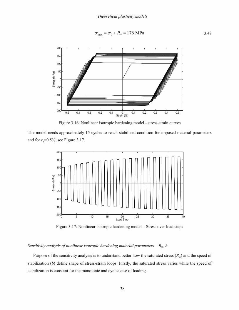
Theoretical plasticity models
38
max 0 176 MPaRσ σ ∞= + = 3.48
Figure 3.16: Nonlinear isotropic hardening model - stress-strain curves
The model needs approximately 15 cycles to reach stabilized condition for imposed material parameters
and for εa=0.5%, see Figure 3.17.
Figure 3.17: Nonlinear isotropic hardening model – Stress over load steps
Sensitivity analysis of nonlinear isotropic hardening material parameters – R∞, b
Purpose of the sensitivity analysis is to understand better how the saturated stress (R∞) and the speed of
stabilization (b) define shape of stress-strain loops. Firstly, the saturated stress varies while the speed of
stabilization is constant for the monotonic and cyclic case of loading.
-0.5 -0.4 -0.3 -0.2 -0.1 0 0.1 0.2 0.3 0.4 0.5-200
-150
-100
-50
0
50
100
150
200
Strain (%)
Stre
ss (M
Pa)
0 5 10 15 20 25 30 35 40-200
-150
-100
-50
0
50
100
150
200
Load Step
Stre
ss (M
Pa)

Theoretical plasticity models
39
Figure 3.18: Sensitivity analysis regarding R∞ for monotonic case of loading
The saturated stress defines the amount of cyclic hardening. For monotonic case of loading (Figure 3.18),
difference between curves in the plastic region is very small due to small amount of the accumulated
plastic strain which is governing parameter in equation 3.40. As can be seen in Figure 3.19, the
accumulated plastic strain increases from cycle to cycle, in case of cyclic loading, simultaneously
affecting on a major difference between curves. The cyclic hardening phenomenon is observed in all three
cases due to positive values of R∞ (38, 76 and 114 MPa).
Figure 3.19: Sensitivity analysis regarding R∞ for cyclic case of loading
In the next phase, the parameter R∞ is constant while three different values (4, 8, 12) of b parameter are
taken into consideration.
0 10 20 30 40 50 60 70 80 90 1000
20
40
60
80
100
120
Load (%)
Stre
ss (M
Pa)
R∞ =38 MPa
R∞* =76 MPa
R∞ =114 MPa
0 5 10 15 20 25 30 35 40
-200
-150
-100
-50
0
50
100
150
200
Load step
Stre
ss (M
Pa)
R∞ =38 MPa
R∞* =76 MPa
R∞ =114 MPa

Theoretical plasticity models
40
Figure 3.20: Sensitivity analysis considering b for cyclic case of loading
The model with the highest imposed value (b=12) reached the stabilized condition earlier with respect to
other two model since b parameter defines the speed of stabilization and accordingly to equation 3.40, see
Figure 3.20.
3.6.3 Combined material model - Armstrong and Frederick’s model and nonlinear
isotropic hardening model
As a final step, the numerical simulation is performed considering the combined material model
(Armstrong and Frederick’s model + nonlinear isotropic hardening model). The combined model is able to
capture simultaneously monotonic hardening and cyclic hardening or softening phenomenon, according to
the theory explained in the paragraph 3.5.3.
The combined material model is defined in the numerical simulation as a combination of Chaboche model
(defining only the one pair of C, γ) and the nonlinear isotropic model. As in previous cases, all material
parameters can be temperature dependent or independent. The material parameters used in analysis are
summarized in Table 3.1. Moreover, temperature independence of material parameters is assumed.
As can be seen in Figure 3.21, changes in the yield surface occur after initial plastic strains, which in this
case affect on translation and on expansion of the yield surface. The monotonic hardening is achieved with
the Armstrong and Frederick’s model which stabilizes in the first cycle. While, the cyclic hardening is
captured with the nonlinear isotropic model which need approximately 15 cycles up to stabilization, see
Figure 3.22.
0 5 10 15 20 25 30 35 40
-200
-150
-100
-50
0
50
100
150
200
Load step
Stre
ss (M
Pa)
b = 4b*= 8b = 12
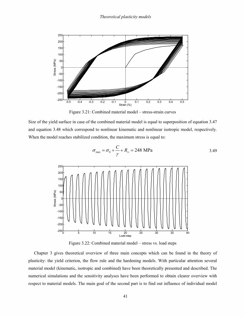
Theoretical plasticity models
41
Figure 3.21: Combined material model – stress-strain curves
Size of the yield surface in case of the combined material model is equal to superposition of equation 3.47
and equation 3.48 which correspond to nonlinear kinematic and nonlinear isotropic model, respectively.
When the model reaches stabilized condition, the maximum stress is equal to:
max 0 248 MPaC Rσ σγ ∞= + + = 3.49
Figure 3.22: Combined material model – stress vs. load steps
Chapter 3 gives theoretical overview of three main concepts which can be found in the theory of
plasticity: the yield criterion, the flow rule and the hardening models. With particular attention several
material model (kinematic, isotropic and combined) have been theoretically presented and described. The
numerical simulations and the sensitivity analyses have been performed to obtain clearer overview with
respect to material models. The main goal of the second part is to find out influence of individual model
-0.5 -0.4 -0.3 -0.2 -0.1 0 0.1 0.2 0.3 0.4 0.5-250
-200
-150
-100
-50
0
50
100
150
200
250
Strain (%)
Stre
ss (M
Pa)
0 5 10 15 20 25 30 35 40-250
-200
-150
-100
-50
0
50
100
150
200
250
Load step
Stre
ss (M
Pa)

Theoretical plasticity models
42
on the material response. The identification procedure of material parameters can be performed once the
theoretical part of the material models is known. Chapter 4 describes methodological approach to estimate
the material parameter for the nonlinear kinematic and the nonlinear isotropic model, as well as the
Young’s modulus and the yield stress.
Experimental testing and estimation of material parameters for CuAg alloy
43
Chapter 4
Experimental testing and estimation of
material parameters for CuAg alloy
Material models, presented in the previous Chapter, are defined with several parameters which is
needed to calibrated from experimental data. Quite often, number of material parameters increases with
increasing the model complexity. Complex numerical algorithms, various methods and optimisation
routines are often used and recommended to identify multiple parameters simultaneously [Broggiato,
2008, Franulović, 2009, Franulović, 2014, Koo, 2011, Pajand, 2009, Tong, 2003, Zaletelj, 2011, Zhao,
2001]. Material characterisation has been missing at the beginning of this work. Therefore, preliminary
material characterization considering isothermal LCF tests seemed to be reasonable to obtained
preliminary results. All material parameters are estimated from isothermal LCF tests.
Chapter 4 is focused on methodology of material characterization. The first section describes the LCF
(low cycle fatigue) tests that were performed on a CuAg alloy at three temperature levels. Moreover,
briefly description of test machines as well as equipment used during the experimental testing is given.
The identification procedure of the yield stress and the Young’s modulus from a first and a stabilized
cycle is explained in the second part of this Chapter. Both parameters should be estimated precisely since
they define the elastic region. Having determined the yield stress and the Young’s modulus, estimation of
the material parameters can be performed for the nonlinear kinematic and the nonlinear isotropic model.
Once all parameters are determined, comparisons between experimental and simulated stress-strain loops
are done in order to evaluate goodness of estimated parameters with respect to used approaches. Obtained
results show satisfactory agreement as could be seen at the end of this Chapter.

Experimental testing and estimation of material parameters for CuAg alloy
44
4.1 Experimental testing
Isothermal low cycle fatigue (LCF) tests were performed to characterize the cyclic stress-strain
behaviour and fatigue life of CuAg alloy at three temperature levels (20 oC, 250 oC and 300 oC).
Experimental testing was performed in the Fatigue Analysis Laboratory at Montanuniversity in Leoben,
where several specimens were tested at different strain ranges at each temperature level. All isothermal
LCF tests were carried out in strain controlled mode with a triangular loading waveform and with a fully
reversed strain ratio:
minε
max
1R εε
= = −
4.1
The examined strain rate was 0.01s-1. Generally, the range of loading frequency for LCF tests is between
0.1 and 1 Hz. The sampling frequency of data shall be at least 200 data points per loop to ensure adequate
definition of stress-strain loop, especially in the region of strain reversal. Tests were interrupted before
specimen failure when the maximal stress decreased by 80%.
Figure 4.1: Shape and dimension of a specimen
Low cycle fatigue tests at 20 oC were performed on the servo-hydraulic Instron-Schenck test rig with a
nominal force ±250 kN (Figure 4.2), while the Instron extensometer with a gauge length of 12.5 mm and a
range of ±5 mm was used to measure elongation during testing, as can be seen in Figure 4.3. Specimens
were clamped by mechanical clamping grips.
0.5x45o
Ø7±
0.02
12020
Ø12
±0.0
5

Experimental testing and estimation of material parameters for CuAg alloy
45
Figure 4.2: Servo-hydraulic Schenck 250 kN test rig
Figure 4.3: Mechanical clamping jaws with extensometer for room temperature
Isothermal LCF testing at 250 oC and 300 oC were performed on the Instron test rig with a nominal force
of ±100 kN. The temperature was applied by the induction heating system with a 10 kW medium
frequency generator, Hüttinger TIG 10/300. The temperature was measured within the gauge length with a
pre-stressed type K loop thermocouple. To measure an elongation at high temperatures the MTS
extensometer, model 632.53F-14 with a gauge length of 12.6 mm and a range of ±1.8 mm was used. Test
specimens were clamped by water cooled hydraulic clamping grips. Hydraulic grips are water cooled in
order to allow quick cyclic stabilization of the longitudinal temperature distribution within the gauge
length and to provide stable thermal condition during the experimental testing. According to ISO 12111
from 2011 year, a temperature of tested specimens near hydraulic grips should be within 15 oC up to 40 oC, depending on a tested temperature. During the performed experimental testing, most of specimens
failed in the middle part where the maximum tested temperatures had appeared.
Figure 4.4: Servo-hydraulic Instron 100 kN test rig
Figure 4.5: Hydraulic clamping jaws, HT extensometer and heating apparatus
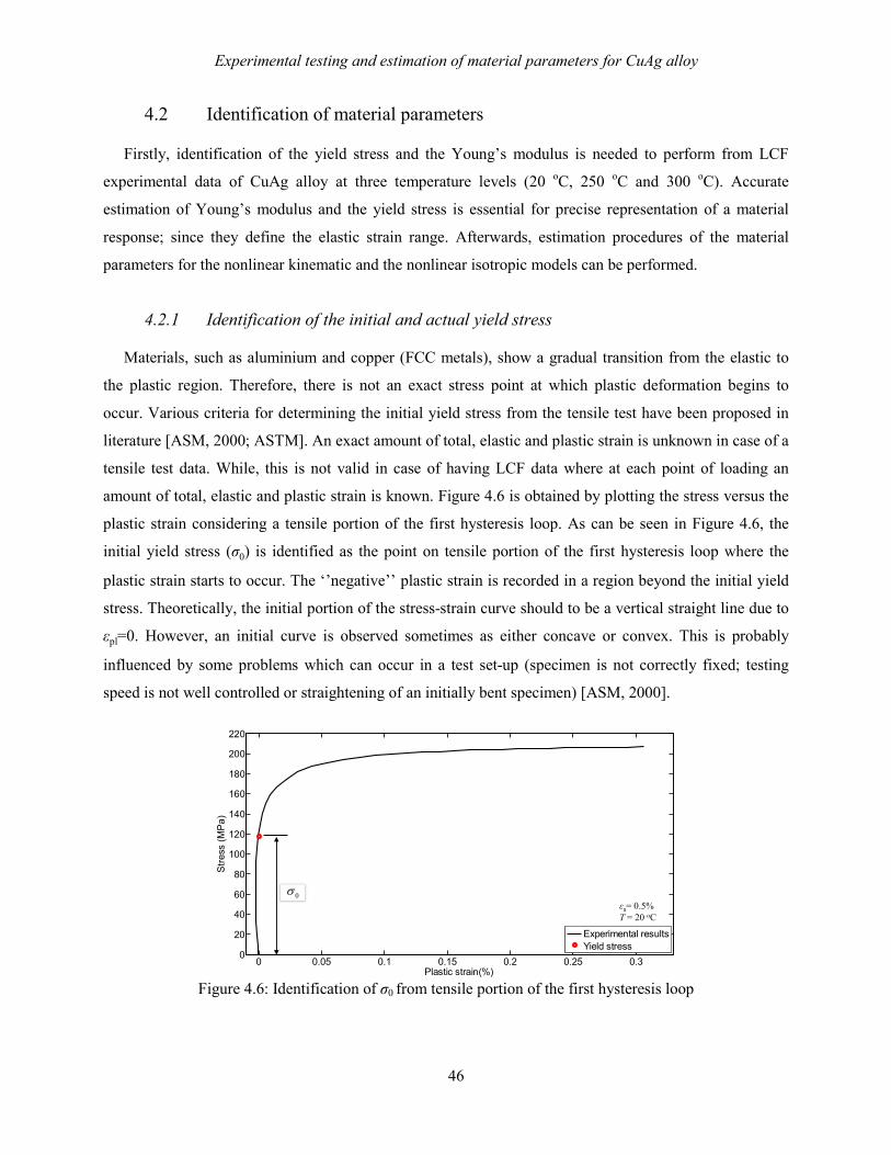
Experimental testing and estimation of material parameters for CuAg alloy
46
4.2 Identification of material parameters
Firstly, identification of the yield stress and the Young’s modulus is needed to perform from LCF
experimental data of CuAg alloy at three temperature levels (20 oC, 250 oC and 300 oC). Accurate
estimation of Young’s modulus and the yield stress is essential for precise representation of a material
response; since they define the elastic strain range. Afterwards, estimation procedures of the material
parameters for the nonlinear kinematic and the nonlinear isotropic models can be performed.
4.2.1 Identification of the initial and actual yield stress
Materials, such as aluminium and copper (FCC metals), show a gradual transition from the elastic to
the plastic region. Therefore, there is not an exact stress point at which plastic deformation begins to
occur. Various criteria for determining the initial yield stress from the tensile test have been proposed in
literature [ASM, 2000; ASTM]. An exact amount of total, elastic and plastic strain is unknown in case of a
tensile test data. While, this is not valid in case of having LCF data where at each point of loading an
amount of total, elastic and plastic strain is known. Figure 4.6 is obtained by plotting the stress versus the
plastic strain considering a tensile portion of the first hysteresis loop. As can be seen in Figure 4.6, the
initial yield stress (σ0) is identified as the point on tensile portion of the first hysteresis loop where the
plastic strain starts to occur. The ‘’negative’’ plastic strain is recorded in a region beyond the initial yield
stress. Theoretically, the initial portion of the stress-strain curve should to be a vertical straight line due to
εpl=0. However, an initial curve is observed sometimes as either concave or convex. This is probably
influenced by some problems which can occur in a test set-up (specimen is not correctly fixed; testing
speed is not well controlled or straightening of an initially bent specimen) [ASM, 2000].
Figure 4.6: Identification of σ0 from tensile portion of the first hysteresis loop
0 0.05 0.1 0.15 0.2 0.25 0.30
20
40
60
80
100
120
140
160
180
200
220
Plastic strain(%)
Stre
ss (M
Pa)
Experimental resultsYield stress
0σεa= 0.5% T = 20 oC

Experimental testing and estimation of material parameters for CuAg alloy
47
The actual yield stress (σ0*) is identified considering the stabilized loop and using the offset method
proposed in [ASM, 2000; ASTM]. However, the offset method has been a little bit modified, since the
original method is proposed for a tensile test data, see Figure 4.7. The offset method is applied in this case
to the stabilized stress-plastic strain loop, see Figure 4.8.
Figure 4.7: Offset Method Figure 4.8: Identification of σ0* from the stabilized hysteresis loop
As can be seen in Figure 4.8, plotting the stress versus the plastic strain for a stabilized cycle, there is not
an exact stress point at which plastic deformation begins to occur. Therefore, the plastic strain offset (for
instance εpl=0.02%) is necessary to define and imposed it at the tip of the loop. The intersection of the
stress-plastic strain curve with the vertical straight line (shifted for εpl=0.02% from tip of the loop) finally
gives the 2σ0* (red dot in Figure 4.8). Concluding, the actual yield stress is identified from the stabilized
loop by plotting the stress versus the plastic strain (Figure 4.8) and using the modified offset method. The
evolution of the yield stress with increasing number of cycles enables to determine the hardening or the
softening characteristics of materials [Hales, 2002]. All estimated values of the initial and the actual yield
stress are listed in Table 4.1-Table 4.3 with respect to testing temperature.
Table 4.1: Estimated values of the initial yield stress and the actual yield stress for T = 20 oC
Yield stress
Strain amplitude (%) Average value 0.15 0.175 0.2 0.3 0.4 0.5 0.6 0.7 1 1.25
σ0 (MPa) 51.3 90.3 95.7 121.6 138.7 118 135.4 155 221.1 174.7 130
σ0* (MPa) 60.5 71.6 87.9 91.4 84.3 88.9 114 86
σ
ε0
A C
B
r
0.002– Specified strain(0.2 %)
*0%2.0 σ
-0.4 -0.3 -0.2 -0.1 0 0.1 0.2 0.3 0.4-200
-150
-100
-50
0
50
100
150
200
Plastic strain (%)
Stre
ss (M
Pa)
Strain offset
εa= 0.5% T = 20 oC
0*2σ

Experimental testing and estimation of material parameters for CuAg alloy
48
Table 4.2: Estimated values of the initial yield stress and the actual yield stress for T = 250 oC
Yield stress
Strain amplitude (%) Average value 0.2 0.3 0.35 0.4 0.5 0.7
σ0 (MPa) 121 111.3 103.4 140.3 80.7 111
σ0* (MPa) 43.1 51.7 50.9 51 53 50
Table 4.3: Estimated values of the initial yield stress and the actual yield stress for T = 300oC
Yield stress
Strain amplitude (%) Average value 0.175 0.2 0.25 0.3 0.4 0.5 0.7
σ0 (MPa) 124 103.3 116.4 122.5 110
σ0* (MPa) 48.3 40.6 48.5 44.7 48.2 40.5 43.5 45
It can be noticed that in all cases σ0* < σ0, confirming softening behaviour of the CuAg alloy at all three
temperature levels (20 oC, 250 oC and 300 oC) and for all strain amplitudes. In addition, the initial yield
stress is temperature dependent parameter, i.e. decreases with increasing the temperature σ0,300 < σ0,250 <
σ0,20 as well as the actual yield stress σ0*,300 < σ0*,250 < σ0*,20. The initial yield stress and actual yield stress
cannot be estimated for some strain amplitudes due to noise which appeared during the experimental
testing.
4.2.2 Identification of the Young’s modulus
The Young’s modulus, as well as the yield stress, is estimated using both the tensile portion of the first
hysteresis loop (E1) and the stabilized stress-strain loop (Es). The Young’s modulus may vary during
testing [Hales, 2002]. Estimation is performed using the linear least square method implemented in Curve
Fitting Toolbox-MATLAB technical computing environment, see Figure 4.9 right. The E1 is determined
using the region beyond the initial yield stress as can be seen in Figure 4.9.
Here the statistical measure R2 is used to judge the adequacy of a regression model. Definition of R2 is
given in Chapter 6.

Experimental testing and estimation of material parameters for CuAg alloy
49
Figure 4.9: Identification of E1 from the first quarter of hysteresis loop
Identification of the Young’s modulus (Es) from the stabilized loop is done using the method proposed by
[Hales, 2002] which suggests fitting of the linear least square method over the defined stress range. The
proposed method is simply to implement, however, the estimated value of Es is very sensitive to the
defined stress range and to the imposed strain offset. The stress range, used during the estimation process,
is defined with two limits: the upper limit is equal to 2σ0* (because the actual yield stress defines the
elastic strain range), while for the lower limit is taken the stress which corresponds to strain offset
(ε=0.01%) imposed at the tip of the loop. Figure 4.10 schematically describes estimation procedure of the
Young’s modulus (Es) from the stabilized loop. Sufficient numbers of stress-strain points is needed to be
recorded within the elastic region in order to estimate Young’s modulus accurately.
Figure 4.10: Identification procedure of Es from the stabilized hysteresis loop
Estimated values of E1 and Es considering several strain amplitudes and three temperature levels are
summarized in Table 4.4 -Table 4.6, respectively. Both Young’s modulus are the function of temperature
E1,300 < E1,250 < E1,20 and Es,300 ≤ Es,250 < Es,20. In addition, they seem to depend on the applied strain
amplitude (εa). Furthermore, the Young’s modulus is slightly decreasing with increasing number of cycles,
0 0.05 0.1 0.15 0.2 0.25 0.3 0.35 0.4 0.45 0.50
50
100
150
200
250
Strain (%)
Stre
ss (M
Pa)
Stress range used for linear
elastic fit εa= 0.5% T = 20 oC
0 0.02 0.04 0.06 0.08 0.1 0.120
20
40
60
80
100
120
Strain (%)
Stre
ss (M
Pa)
Experimental resultEstimated results
2 0.99R =
εa= 0.5% T = 20 oC
-0.5 -0.4 -0.3 -0.2 -0.1 0 0.1 0.2 0.3 0.4 0.5-200
-150
-100
-50
0
50
100
150
200
Strain (%)
Stre
ss (M
Pa)
Stress range used for linear
elastic fit
Strain offset εa= 0.5% T = 20 oC
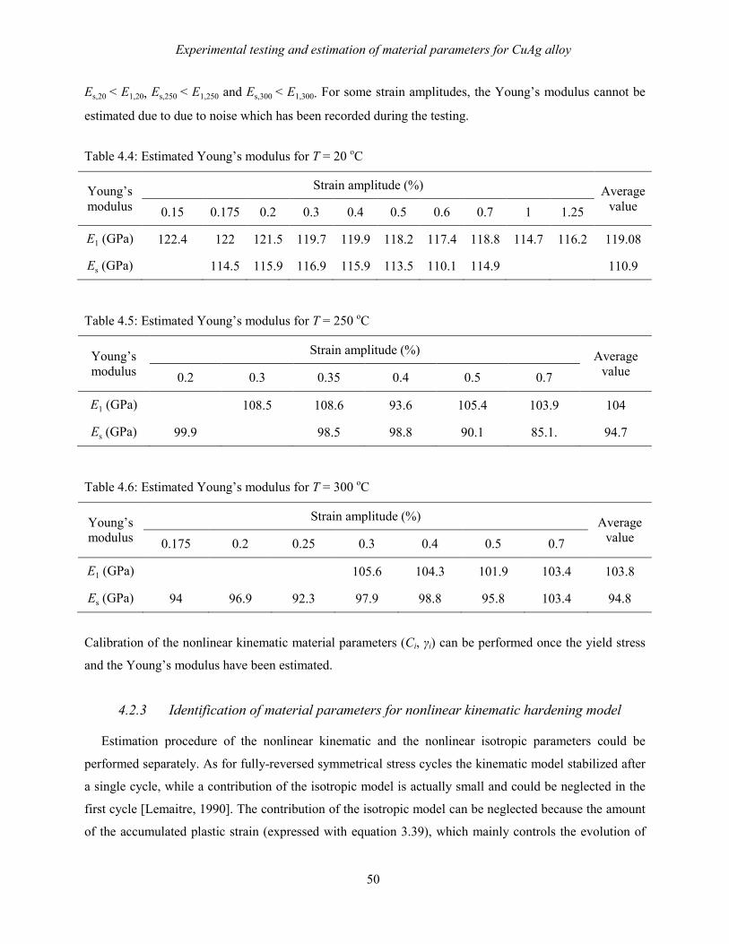
Experimental testing and estimation of material parameters for CuAg alloy
50
Es,20 < E1,20, Es,250 < E1,250 and Es,300 < E1,300. For some strain amplitudes, the Young’s modulus cannot be
estimated due to due to noise which has been recorded during the testing.
Table 4.4: Estimated Young’s modulus for T = 20 oC
Young’s modulus
Strain amplitude (%) Average value 0.15 0.175 0.2 0.3 0.4 0.5 0.6 0.7 1 1.25
E1 (GPa) 122.4 122 121.5 119.7 119.9 118.2 117.4 118.8 114.7 116.2 119.08
Es (GPa) 114.5 115.9 116.9 115.9 113.5 110.1 114.9 110.9
Table 4.5: Estimated Young’s modulus for T = 250 oC
Young’s modulus
Strain amplitude (%) Average value 0.2 0.3 0.35 0.4 0.5 0.7
E1 (GPa) 108.5 108.6 93.6 105.4 103.9 104
Es (GPa) 99.9 98.5 98.8 90.1 85.1. 94.7
Table 4.6: Estimated Young’s modulus for T = 300 oC
Young’s modulus
Strain amplitude (%) Average value 0.175 0.2 0.25 0.3 0.4 0.5 0.7
E1 (GPa) 105.6 104.3 101.9 103.4 103.8
Es (GPa) 94 96.9 92.3 97.9 98.8 95.8 103.4 94.8
Calibration of the nonlinear kinematic material parameters (Ci, γi) can be performed once the yield stress
and the Young’s modulus have been estimated.
4.2.3 Identification of material parameters for nonlinear kinematic hardening model
Estimation procedure of the nonlinear kinematic and the nonlinear isotropic parameters could be
performed separately. As for fully-reversed symmetrical stress cycles the kinematic model stabilized after
a single cycle, while a contribution of the isotropic model is actually small and could be neglected in the
first cycle [Lemaitre, 1990]. The contribution of the isotropic model can be neglected because the amount
of the accumulated plastic strain (expressed with equation 3.39), which mainly controls the evolution of

Experimental testing and estimation of material parameters for CuAg alloy
51
the isotropic model, is negligible small in the first cycle and increases with number of cycles. Moreover,
the kinematic model is the one which defines the shape of the hysteresis loop. Obviously, way by which
the material parameters are determined depends significantly on availability of experimental data. Three
different identification methods are adopted and presented in addition:
1) using a single tension curve,
2) using a single stabilized stress-strain hysteresis loop and
3) using several stabilized stress-strain hysteresis loops.
4.2.3.1 Identification from single tension curve Approximate parameters of Ci and γi can be estimated using a single tension curve, see Figure 4.11.
However, this approach is not recommended since there are no cyclic data with which to correlate the
parameters [Imaoka, 2008]. Having only a tensile test data, an amount of the total strain is known, while
an amount of the elastic and plastic strain is unknown. The identification procedure of Ci and γi should be
performed based on the stress versus the plastic strain data, but this cannot be done since an amount of the
plastic strain is unknown. However, subtracting the initial yield stress from the overall stress (red dot on
the Figure 4.11) gives the stress-strain distribution (red line on the Figure 4.11) which should be converted
to the back stress by shifting the obtained stress-strain to the origin of the coordinate system.
Figure 4.11: Identification of Ci and γi from a single tension curve
Material parameters are possible to identify with respect to obtained stress-strain data and using equation
(3.25). This approach may be suitable for situations when is needed to simulate only a few cycles
[Imaoka, 2008], however, in any case obtained results should be taken with additional reserve of caution.
0 0.05 0.1 0.15 0.2 0.25 0.3 0.35 0.4 0.45 0.50
20
40
60
80
100
120
140
160
180
200
220
Strain (%)
Stre
ss (M
Pa)
0σ

Experimental testing and estimation of material parameters for CuAg alloy
52
4.2.3.2 Identification from a single stabilized cycle Identification of material parameters (Ci, γi) can be performed using a single stabilized stress-strain
hysteresis loop. Estimated parameters are appropriate to use for particular strain amplitude that has been
used during the identification procedure. Firstly, the elastic and the plastic part are necessary to identify
using the stabilized stress-strain loop as a starting point. The actual yield stress that defines the elastic
region for stabilized cycle is used to separate the elastic and the plastic part. Additionally, the plastic strain
range and the stress range are needed to measure. The plastic part (the back stress) is obtained by
subtracting the actual yield stress from the upper branch (i.e. α=Δσ/2 - σ0*). Moreover, the plastic part
should be shifted to the origin of the coordinate system. Shifting is done due to facilitate implementation
of the nonlinear least square method. Calculation steps described until now are presented in Figure 4.12.
Figure 4.12: Stress vs. plastic strain for a single stabilized cycle
Equation (3.25) is appropriate to use in order to identify parameters (Ci, γi) from a single stabilized cycle.
Elaboration of the data is performed with the Curve Fitting Toolbox. The Curve Fitting Toolbox has
possibility of writing custom equation that becomes base for the nonlinear least square method. Moreover,
the Toolbox has option to define the initial starting points as well as the upper and the lower bounds. The
initial values of Cin and γin are imposed as the initial starting points. The slope after the yield stress is
assumed to be Cin while γin is obtained through the relation Cin/γin, see Figure 4.12.
Figure 4.13 shows fitting between the experimental data and superposition of three determined back
stresses. The first pair (C1, γ1 - dashed line) achieves stabilization very fast due to very high γ1. The initial
hardening modulus (C1) decreases more with higher value of γ1, since the nonlinear recall parameter (γ)
defines a rate at which C starts to decrease with increasing the plastic strain. The second pair (C2, γ2 – dash
dot line) has smaller γ2 and archives the maximum stress (i.e. stabilization) after the first pair. The third
-0.4 -0.3 -0.2 -0.1 0 0.1 0.2 0.3 0.4 0.5 0.6-200
-150
-100
-50
0
50
100
150
200
Plastic strain (%)
Stre
ss (M
Pa)
0*2σ
in inC γ
inC

Experimental testing and estimation of material parameters for CuAg alloy
53
pair (C3, γ3 – dotted line) has the highest maximum stress (σmax=C3/γ3) that has been reached after the
second and the third pair due to γ1> γ2> γ3. The second pair has the greater slope and stabilizes earlier than
the third pair. The material parameters used during the estimation procedure are summarized in the Table
4.7. Sum of all three back stresses gives the final curve (solid line) which shows goodness of fitting
regarding experimental data.
Figure 4.13: Superposition of three nonlinear kinematic hardening models – T = 20 oC
Superposition of two nonlinear kinematic hardening models gives the good agreement regarding the
experimental, as can be seen in Figure 4.14. The first pair has a greater slope and stabilizes faster than the
second pair because C1 > C2 and γ1 > γ2, see Table 4.7. The statistical measure, R2=0.9998, shows precisely
fitting between the experimental data and the calculated back stress.
Figure 4.14: Superposition of two nonlinear kinematic hardening models – T = 20 oC
0 0.1 0.2 0.3 0.4 0.5 0.6 0.70
50
100
150
Test dataα1α2α3α
( )11 1 pl
1
1 expCα γ εγ
= − −
( )22 2 pl
2
1 expCα γ εγ
= − −
( )33 3 pl
3
1 expCα γ εγ
= − −
1 2 3α α α α= + +
2 0.9999R =
pl (%)ε∆
0 0.1 0.2 0.3 0.4 0.5 0.6 0.70
50
100
150
Test dataα1α2α
1 2α α α= +
2 0.9998R =( )1
1 1 pl1
1 expCα γ εγ
= − −
( )22 2 pl
2
1 expCα γ εγ
= − −
pl (%)ε∆

Experimental testing and estimation of material parameters for CuAg alloy
54
Figure 4.15 shows the correlation between the experimental data and the back stress obtained with just one
pair of material parameters. In this case, the fitting is not so precisely, R2=0.9787, as in the previous two
cases with two and three pairs of material parameters.
Figure 4.15: Nonlinear kinematic hardening model with one pair of material parameters – T = 20 oC
Parameters determined with the second method and considering the experimental data εa=0.5% at 20 oC
are summarized in Table 4.7.
Table 4.7: Nonlinear kinematic hardening parameters (Ci, γi) - T = 20 oC
Stain amplitude – 0.5%
C1 (MPa) γ1 C2 (MPa) γ2 C3 (MPa) γ3
Three pairs 1089000 661700 76370 3163 23970 492.8
Two pairs 90420 3779 25830 514.2
One pair 66000 943
In addition, the material parameters (Ci, γi) are estimated using the second already explained identification
method and considering the LCF data with εa=0.5% at 250 oC.
Figure 4.16 -Figure 4.18 show correlation between the LCF data and the back stresses obtained with 3, 2
and 1 pair of material parameters, respectively. Figure 4.16 present fitting between the experimental data
and the superposition of three nonlinear kinematic models. The first pair has the highest slope and
achieves the stabilization faster than two other curves due to C1 > C2 > C3 and γ1 > γ2 > γ3, see Table 4.8.
0 0.1 0.2 0.3 0.4 0.5 0.6 0.70
50
100
150
Test dataα1
2 0.9787R =
( )11 1 pl
1
1 expCα γ εγ
= − −
pl (%)ε∆

Experimental testing and estimation of material parameters for CuAg alloy
55
Figure 4.16: Superposition of three nonlinear kinematic hardening models – T=250 oC
The good agreement is also achieved with the superposition of two nonlinear kinematic hardening models.
As can be seen in Table 4.8, the curve calculated with first pair has a greater slope and stabilizes faster
than the second pair due to C1 > C2 and γ1 > γ2.
Figure 4.17: Superposition of two nonlinear kinematic hardening models – T = 250 oC
Fitting between the experimental data and the back stress obtained with only one pair gives satisfactory
agreement. The R2 is the lowest regarding two previous cases. The best correlation between experimental
and calculated back stress is obtained with 3 pairs as in case of LCF experimental data at 20 oC.
0 0.1 0.2 0.3 0.4 0.5 0.6 0.7 0.80
20
40
60
80
100
120
Plastic strain (%)
Stre
ss (M
Pa)
Experimental curveα1α2α3α1+α2+α3
( )11 1 pl
1
1 expCα γ εγ
= − −
( )22 2 pl
2
1 expCα γ εγ
= − − ( )33 3 pl
3
1 expCα γ εγ
= − −
1 2 3α α α α= + +
pl (%)ε∆
9994.02 =R
0 0.1 0.2 0.3 0.4 0.5 0.6 0.7 0.80
20
40
60
80
100
120
Test dataα1α2α
( )11 1 pl
1
1 expCα γ εγ
= − −
( )22 2 pl
2
1 expCα γ εγ
= − −
1 2 3α α α α= + +
pl (%)ε∆
9993.02 =R

Experimental testing and estimation of material parameters for CuAg alloy
56
Figure 4.18: Nonlinear kinematic hardening model with one pair of material parameters – T = 250 oC
Table 4.8 summarized the material parameters identified from the LCF data with respect to εa=0.5% at
250oC.
Table 4.8: Nonlinear kinematic hardening parameters (Ci, γi) - T = 250 oC
Stain amplitude – 0.5%
C1 (MPa) γ1 C2 (MPa) γ2 C3 (MPa) γ3
Three pairs 59780 4647 23480 1132 7758 379.4
Two pairs 67230 3315 17970 554.9
One pair 52000 1020
In addition, material parameters are estimated from LCF data with εa=0.5% at 300 oC by applying the
identification procedure explained in case T = 20 oC
Figure 4.19 -Figure 4.21 present fitting between the experimental and estimated back stresses with 3, 2
and 1 pair of material parameters, respectively. Also in this case, the best correlation is obtained with 3
pairs, while with only 1 pair of parameters is obtained not so precise fitting between experimental and
calculated back stress.
0 0.1 0.2 0.3 0.4 0.5 0.6 0.7 0.80
20
40
60
80
100
120
Test dataα1
pl (%)ε∆
( )11 1 pl
1
1 expCα γ εγ
= − −
9786.02 =R

Experimental testing and estimation of material parameters for CuAg alloy
57
Figure 4.19: Superposition of three nonlinear kinematic hardening models – T=300 oC
Figure 4.20: Superposition of two nonlinear kinematic hardening models – T = 300 oC
Figure 4.21: Nonlinear kinematic hardening model with one pair of material parameters – T = 300 oC
0 0.1 0.2 0.3 0.4 0.5 0.6 0.7 0.80
20
40
60
80
100
120
Plastic strain (%)
Stre
ss (M
Pa)
Experimental curveα1α2α3α1+α2+α3
( )11 1 pl
1
1 expCα γ εγ
= − −
( )22 2 pl
2
1 expCα γ εγ
= − −
( )33 3 pl
3
1 expCα γ εγ
= − −
1 2 3α α α α= + +
pl (%)ε∆
9986.02 =R
0 0.1 0.2 0.3 0.4 0.5 0.6 0.7 0.80
20
40
60
80
100
120
Test dataα1α2α
2 0.9787R =( )1
1 1 pl1
1 expCα γ εγ
= − −
( )22 2 pl
2
1 expCα γ εγ
= − −
1 2 3α α α α= + +
pl (%)ε∆
9983.02 =R
0 0.1 0.2 0.3 0.4 0.5 0.6 0.7 0.80
20
40
60
80
100
120
Test dataα1
pl (%)ε∆
( )11 1 pl
1
1 expCα γ εγ
= − −
9706.02 =R

Experimental testing and estimation of material parameters for CuAg alloy
58
Material parameters determined from LCF data with εa=0.5% measured at 300 oC are summarized in Table
4.9
Table 4.9: Nonlinear kinematic hardening parameters (Ci, γi) - T = 300 oC
Stain amplitude – 0.5%
C1 (MPa) γ1 C2 (MPa) γ2 C3 (MPa) γ3
Three pairs 108800 7906 31760 1337 8437 427.3
Two pairs 110000 5396 24390 681
One pair 68420 1264
Comparison between experimental stabilized stress-strain loops and simulated loops is performed to
assess quality of estimated material parameters. Numerical simulations are performed adopting the
example described in paragraph 3.6. Values of the Young’s modulus (Es) and the actual yield stress (σ0*)
used in simulation correspond to values estimated from LCF data with εa=0.5% at 20 oC.
Figure 4.22 shows comparison between the experimental and simulated stress-strain loops with 1, 2 and 3
pairs of parameters with respect to data at 20 oC, see Table 4.7. A better agreement, in the middle part of
stress-strain loop, is obtained using two and three pairs of material parameters while results obtained with
just one pair do not show such good agreement. Furthermore, simulated stress-strain loops obtained with
two and three pairs overlap each other. All three simulated hysteresis approximately coincide (±1 MPa) to
experimental loop in case that peaks of loops are observed.
Figure 4.22: Comparison between experimental and simulated stress-strain loops – T = 20 oC
-0.5 -0.4 -0.3 -0.2 -0.1 0 0.1 0.2 0.3 0.4 0.5-200
-150
-100
-50
0
50
100
150
200
Strain (%)
Stre
ss (M
Pa)
Experimental hysteresisSimulated hysteresis 1 pairSimulated hysteresis 2 pairsSimulated hysteresis 3 pairs
εa= 0.5% T = 20 oC

Experimental testing and estimation of material parameters for CuAg alloy
59
In addition, Figure 4.23 shows fitting between the experimental and simulated stress-strain loops with 1, 2
and 3 pairs of parameters with respect to data at 250 oC, see Table 4.8. The better fitting, considering the
middle part of the loop, is obtained with loops that correspond to 2 and 3 pairs of parameters. However, all
three simulated loops coincide to experimental loop ±1 MPa in the peaks.
Figure 4.23: Comparison between experimental and simulated hysteresis – T = 250 oC
The last comparison takes into consideration the experimental data and material parameter with respect to
T=300 oC, see Table 4.9. Fitting between the experimental stabilized loop and simulated stress-strain loops
obtained with 2 and 3 pair, considering the middle part, is better than with the loop gained with one pair.
Also in this case, all three simulated loops coincide to experimental loop ±1 MPa in peaks.
Figure 4.24: Comparison between experimental and simulated hysteresis – T = 300 oC
-0.5 -0.4 -0.3 -0.2 -0.1 0 0.1 0.2 0.3 0.4 0.5-200
-150
-100
-50
0
50
100
150
200
Strain (%)
Stre
ss (M
Pa)
Experimental hysteresisSimulated hysteresis 1 pairSimulated hysteresis 2 pairsSimulated hysteresis 3 pairs
εa= 0.5% T = 250 oC
-0.5 -0.4 -0.3 -0.2 -0.1 0 0.1 0.2 0.3 0.4 0.5-200
-150
-100
-50
0
50
100
150
200
Strain (%)
Stre
ss (M
Pa)
Experimental hysteresisSimulated hysteresis 1 pairSimulated hysteresis 2 pairsSimulated hysteresis 3 pairs
εa= 0.5% T = 300 oC

Experimental testing and estimation of material parameters for CuAg alloy
60
4.2.3.3 Identification from several stabilized cycles The method proposed by [Lemaitre, 1990] suggests using several stabilized hysteresis loops that
correspond to different strain amplitudes. Material parameters determined with this method are suitable to
be used for different strain amplitudes. Identically with a previous method (see paragraph 4.2.3.2), the
plastic strain range (Δεpl) and the stress range (Δσ) are necessary to calculate for each stabilized stress-
strain loop.
Figure 4.25: Stress vs. plastic strain
The elastic domain (2σ0*) is roughly 160 MPa considering Figure 4.25 which shows the stabilized stress-
strain loop for εa=0.5% at 20 oC. Furthermore, the stress range is equal to 306 MPa and the plastic strain
range is 0.69%. Subtracting the actual yield stress (σ0*) from the stress amplitude gives the point presented
in Table 4.10. Repeating the same procedure for each strain amplitude, finally gives the points listed in
Table 4.10 and plotted in Figure 4.26. The fitting procedure, using equation (3.35), is performed for one
and two pairs of material parameters. The initial values Cin and γin are calculated from Figure 4.26 as an
asymptotic value C/γ ≈ 77 MPa. Subsequently, the initial hardening modulus (Cin) is calculated to be
approximately 166500 MPa while γin=2162 is obtained through relation C/γ. As with the second method,
the fitting procedure is done using the Curve Fitting Toolbox in MATLAB.
-0.4 -0.3 -0.2 -0.1 0 0.1 0.2 0.3 0.4-200
-150
-100
-50
0
50
100
150
200
Plastic strain (%)
Stre
ss (M
Pa)
εa= 0.5% T = 20 oC
plε∆
σ∆
0*2σ

Experimental testing and estimation of material parameters for CuAg alloy
61
Table 4.10: Points measured from LCF data at T = 20 oC
Strain amplitude (%)
0.2 0.3 0.4 0.5 0.6 0.7
σa-σ0* (MPa) 46 54.5 63.5 73 75 77
εa (%) 0.1 0.16 0.25 0.345 0.44 0.53
Figure 4.26 shows the fitting procedure between calculated points listed in Table 4.10 and curves obtained
with 1 and 2 pairs of parameters. As can been noticed, a better correlation between experimental points
and fitted curves is obtained with only one pair (C1, γ1).
Figure 4.26: Curve fitting with the method of least squares, using data of 6 hysteresis loops - T = 20 oC
One and two pairs of material parameters are estimated considering 5 different strain amplitudes at 250 oC
and using the same methodological approach explained earlier. Measured points base on which is
performed the nonlinear least square fitting procedure are summarized in Table 4.11.
Table 4.11: Points measured from LCF data at T = 250 oC
Strain amplitude (%)
0.2 0.3 0.4 0.5 0.7
σa-σ0* (MPa) 44.6 45.5 55 57.1 56.4
εa (%) 0.12 0.21 0.3 0.39 0.59
0 0.1 0.2 0.3 0.4 0.5 0.6 0.70
10
20
30
40
50
60
70
80
εpl,a (%)
σ a - σ0*
(MP
a)
Data from 6 TestCurve-Fit Parameters - 1 pairCurve-Fit Parameters - 2 pairs
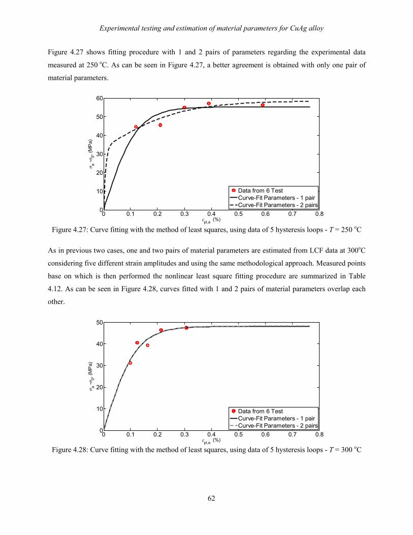
Experimental testing and estimation of material parameters for CuAg alloy
62
Figure 4.27 shows fitting procedure with 1 and 2 pairs of parameters regarding the experimental data
measured at 250 oC. As can be seen in Figure 4.27, a better agreement is obtained with only one pair of
material parameters.
Figure 4.27: Curve fitting with the method of least squares, using data of 5 hysteresis loops - T = 250 oC
As in previous two cases, one and two pairs of material parameters are estimated from LCF data at 300oC
considering five different strain amplitudes and using the same methodological approach. Measured points
base on which is then performed the nonlinear least square fitting procedure are summarized in Table
4.12. As can be seen in Figure 4.28, curves fitted with 1 and 2 pairs of material parameters overlap each
other.
Figure 4.28: Curve fitting with the method of least squares, using data of 5 hysteresis loops - T = 300 oC
0 0.1 0.2 0.3 0.4 0.5 0.6 0.7 0.80
10
20
30
40
50
60
εpl,a (%)
σ a - σ0*
(MP
a)
Data from 6 TestCurve-Fit Parameters - 1 pairCurve-Fit Parameters - 2 pairs
0 0.1 0.2 0.3 0.4 0.5 0.6 0.7 0.80
10
20
30
40
50
εpl,a (%)
σ a - σ0*
(MP
a)
Data from 6 TestCurve-Fit Parameters - 1 pairCurve-Fit Parameters - 2 pairs

Experimental testing and estimation of material parameters for CuAg alloy
63
Table 4.12: Points measured from LCF data at T = 300 oC
Strain amplitude (%)
0.175 0.2 0.25 0.3 0.5
σa-σ0* (MPa) 31.2 40.6 39.5 46.4 37.4
εa (%) 0.1 0.125 0.163 0.21 0.31
One and two pairs of material parameters estimated from LCF experimental data for three temperature
levels (20 oC, 250 oC, 300 oC) are summarized in Table 4.13
Table 4.13: Material parameter estimated using the third method
Temp. One pair Two pairs
C1 (MPa) γ1 C1 (MPa) γ1 C2 (MPa) γ2
20 oC 46250 617.2 38160 505.7 679.5 274
250 oC 45340 820.9 290600 8699 8772 349.5
300 oC 40080 832.8 27530 894.9 12760 731.1
Figure 4.29 - Figure 4.30 show comparison between experimental stabilized loops and stress-strain loops
calculated with the numerical simulations. The numerical simulations are performed adopting the example
described in paragraph 3.6 and using the average values of the Young’s modulus and the actual yield
stress. The simulations are done considering one and two pairs of material parameters estimated at 20 oC,
250 oC and 300oC, respectively.
As can be seen in Figure 4.29, better agreement between the experimental and simulated stress-strain
loops is obtained with only one pair at 20 oC, 250 oC; while at 300oC one and two pairs give quite the same
shape of stress-stain loops.

Experimental testing and estimation of material parameters for CuAg alloy
64
a)
b)
c)
Figure 4.29: Comparison between experimental and simulated stress-strain loops at different temperatures, εa=0.5%
Figure 4.30 shows comparison between experimental and simulated stress-strain loops considering
different strain amplitudes (εa). The comparison is performed in order to confirm that the estimated
material parameters are suitable to be used over wider interval of strain ranges. As can be seen in Figure
-0.5 -0.4 -0.3 -0.2 -0.1 0 0.1 0.2 0.3 0.4 0.5
-150
-100
-50
0
50
100
150
ε (%)
σ (M
Pa)
Experimental stabilized stress-strain loopSimulated stress-strain loop - 1 pairSimulated stress-strain loop - 2 pairs
o
a
20 C0.5%
Tε==
-0.5 -0.4 -0.3 -0.2 -0.1 0 0.1 0.2 0.3 0.4 0.5
-150
-100
-50
0
50
100
150
ε (%)
σ (M
Pa)
Experimental stabilized stress-strain loopSimulated stress-strain loop - 1 pairSimulated stress-strain loop - 2 pairs
o
a
250 C0.5%
Tε==
-0.5 -0.4 -0.3 -0.2 -0.1 0 0.1 0.2 0.3 0.4 0.5
-150
-100
-50
0
50
100
150
ε (%)
σ (M
Pa)
Experimental stabilized stress-strain loopSimulated stress-strain loop - 1 pairSimulated stress-strain loop - 2 pairs
o
a
300 C0.5%
Tε==

Experimental testing and estimation of material parameters for CuAg alloy
65
4.30, a quite good matching with the experimental data characterizes all three cases. Based on the obtained
results, it is possible to conclude that nonlinear kinematic model with one pair of the material parameters
(e.g. the Armstrong and Frederick’s model) gives the best agreement regarding experimental data.
Therefore, the Armstrong and Frederick’s model is going to be used in following simulations.
a)
b)
c) Figure 4.30: Comparison between experimental and simulated stress-strain loops at
different strain amplitudes, T=20 oC
-0.3 -0.2 -0.1 0 0.1 0.2 0.3
-150
-100
-50
0
50
100
150
ε (%)
σ (M
Pa)
Experimental stabilized stress-strain loopSimulated stress-strain loop - 1 pair
o
a
20 C0.3%
Tε==
-0.4 -0.3 -0.2 -0.1 0 0.1 0.2 0.3 0.4
-150
-100
-50
0
50
100
150
ε (%)
σ (M
Pa)
Experimental stabilized stress-strain loopSimulated stress-strain loop - 1 pair
o
a
20 C0.4%
Tε==
-0.6 -0.5 -0.4 -0.3 -0.2 -0.1 0 0.1 0.2 0.3 0.4 0.5 0.6
-150
-100
-50
0
50
100
150
ε (%)
σ (M
Pa)
Experimental stabilized stress-strain loopSimulated stress-strain loop - 1 pair
o
a
20 C0.6%
Tε==

Experimental testing and estimation of material parameters for CuAg alloy
66
Figure 4.26, Figure 4.27 and Figure 4.28 show that fitting between experimental data and estimated
parameters are not so precisely, however, when the estimated material parameters are used to gain
simulated stress-strain loops the fitting between experimental stabilized loop and simulated loops become
satisfactory in all cases, see Figure 4.29 and Figure 4.30. It is important to note that on the overall result
(fitting between experimental and simulated loops) significantly affect not just accuracy of evaluated
material parameters but also accuracy of estimated the Young’s modulus and the yield stress.
Table 4.14 shows goodness of fitting considering the material parameters estimated with the second
(single stabilized cycle) and the third (several stabilized cycles) method. Evaluation is performed using
statistical measures (R2 and SSE). Firstly, the parameters estimated for εa=0.2% with the second method
are compared regarding εa=0.2%, εa=0.5% and εa=0.7%, respectively. Then, the parameters obtained for
εa=0.5% and εa=0.7% using the second method are compared with εa=0.2%, εa=0.5% and εa=0.7%,
respectively. At the end, material parameters estimated with the third method are compared regarding
εa=0.2%, εa=0.5% and εa=0.7%.
Statistical measures R2 and SSE are explained in Chapter 6. R2 can take on any value between 0 and 1,
with a value closer to 1 indicating that a greater proportion of variance is accounted for by the model.
While SSE measures the total deviation of the response values from the fit to the response values. A value
closer to 0 indicates that the model has a smaller error component, and that the fit will be more useful for
prediction.
Table 4.14: Comparison between second and third method
Strain amplitude (%) Second Method Third Method
a 0.2ε = a 0.5ε = a 0.7ε = a 0.2 0.7ε = ÷
a 0.2ε = SSE 208.3 7914.3 13261 3687.6
R2 0.9952 0.8180 0.6951 0.9152
a 0.5ε = SSE 86961.4 2380.2 5837.4 8313.3
R2 0.2203 0.9787 0.9476 0.9255
a 0.7ε = SSE 157960 7560.6 3356.4 10707
R2 0.4483 0.9307 0.9692 0.9018
For an example, considering the second method (single stabilized cycle) and εa=0.2% (Table 4.14), it can
be noticed that fitting is quite precisely for εa=0.2% (SSE=208.3 and R2=0.9952); which has been used to
estimate material parameters. However, using these parameters for εa=0.5% and εa=0.7% give a poor

Experimental testing and estimation of material parameters for CuAg alloy
67
fitting in both cases (i.e., SSE0.2%=208.3 < SSE0.5%=86961.4 < SSE0.7%=157960 and R20.2%=0.9952 >
R20.7%=0.4483 > R2
0.5%=0.2203). On the other hand, material parameters estimated using the third method
(several stabilized cycles) fit quite precisely for all 3 strain amplitudes, i.e. in all 3 cases the R2>0.99.
Based on obtained results, it is possible to conclude that using the third method to estimate just one pair of
material parameters gives satisfactory correlation between experimental and simulated stress strain loops.
It is important to note that parameters obtained with several stabilized cycles method cover wider strain
range. However, the disadvantage of third method is that it requires a sufficient number of experimental
data to obtain representative parameters.
4.2.4 Identification of material parameters for nonlinear isotropic hardening model
The nonlinear isotropic hardening model has two material parameters saturation stress (R∞) and speed
of stabilization (b) to be estimated from LCF data. The saturation stress indicates an amount of hardening
or softening and it is determined as the difference in the maximum stress of the first cycle (σmax,1) and the
stabilized one (σmax,s). As can be noticed in Figure 4.31, Figure 4.33 and Figure 4.35, the saturation stress
depends on the applied strain amplitude, contrary to the assumption of the nonlinear isotropic model in
Equation (3.40). CuAg alloy shows a softening behaviour.
Figure 4.31: Maximum stress as the function of number of cycles - T = 20 oC
100 101 102 103 104 1050
50
100
150
200
250
300
Number of cycles, N
σ max
(MP
a)
εa=0.175%
εa=0.2%
εa=0.3%
εa=0.4%
εa=0.5%
εa=0.6%
εa=0.7%
εa=1%
εa=1.25%

Experimental testing and estimation of material parameters for CuAg alloy
68
The speed of stabilization is estimated using the relation (3.43) proposed by [Chaboche, 2008, Lemaitre,
1990, Lemaitre, 2005]:
( ) ( )NbbRRi
placcpl,1max,smax,
1max,max, 2exp1exp1 εεσσσσ
∆−−=−−=≈−−
∞
If Δεpl is the plastic strain range over a cycle, the accumulated plastic strain for N cycles is εpl,acc≈2ΔεplN.
As can be seen in Figure 4.32, Figure 4.34, Figure 4.36, a reasonable correlation is obtained, although a
modification of the evolution rule of R seems necessary for CuAg alloy; since the relation (3.43) was
originally used for steel 316 in [Lemaitre, 1990]. This kind of behaviour was also observed in [Zhao,
2001] for a nickel based superalloy. One of the future plans could be to create a new relation which is able
to give a better fitting. However, a new relation is necessary to implement in the finite element numerical
software what requires addition work. Obtained values of R∞ and b for each strain amplitude are
summarized in Table 4.15.
Figure 4.32: The identification of the isotropic parameter b - T = 20 oC
Table 4.15: Estimated isotropic parameters for T = 20 oC
Parameter Strain amplitude (%) Average
value 0.175 0.2 0.3 0.4 0.5 0.6 0.7 1 1.25
R∞ (MPa) -58.1 -80.9 -84.4 -83.2 -52.1 -54.1 -69 -96.1 -103.9 -75.7
b 1.197 3.724 3.620 4.488 2.871 2.580 4.208 1.192 0.840 2.352
10-2 10-1 100 101
0
0.2
0.4
0.6
0.8
1
εa=0.175%
εa=0.2%
εa=0.3%
εa=0.4%
εa=0.5%
εa=0.6%
εa=0.7%
εa=1%
εa=1.25%

Experimental testing and estimation of material parameters for CuAg alloy
69
The material parameters (R∞, b) are estimated from experimental data for temperature levels 250 oC and
300 oC using the methodological approach explained earlier. Plotting the maximum stress versus number
of cycles is possible to determine the amount of the saturated stress (R∞), as can be seen in Figure 4.33.
The CuAg alloy shows the cyclic softening behaviour also on T=250 oC. Figure 4.34 represents fitting
procedure of b parameter. Both parameters (R∞, b) are estimated considering 5 different strain amplitudes
measured at 250 oC. As it has been explained earlier, modification of the evolution rule of R seems
necessary for CuAg.
Figure 4.33: Maximum stress as the function of number of cycles - T = 250 oC
Figure 4.34: The identification of the isotropic parameter b - T = 250 oC
100 101 102 103 104 1050
50
100
150
200
250
300
Number of cycles, N
σ max
(MP
a)
εa=0.2%
εa=0.3%
εa=0.4%
εa=0.5%
εa=0.7%
10-2 10-1 100 101
0
0.2
0.4
0.6
0.8
1
εa=0.2%
εa=0.3%
εa=0.4%
εa=0.5%
εa=0.7%

Experimental testing and estimation of material parameters for CuAg alloy
70
Estimated values of R∞ and b from LCF data at 250 oC are summarized in Table 4.16.
Table 4.16: Estimated isotropic parameters for T = 250 oC
Parameter Strain amplitude (%) Average
value 0.2 0.3 0.4 0.5 0.7
R∞ (MPa) -84 -76.5 -93 -90.9 56.4 -80.2
b 5.395 3.898 5.099 5.780 1.484. 3.894
Identification procedure of isotropic parameters (R∞, b) is demonstrated in Figure 4.35 and Figure 4.36,
respectively, considering 5 different strain amplitudes measured at 300 oC. As can be seen in Figure 4.35,
CuAg alloy shows the cyclic softening behaviour also on T=300 oC. Figure 4.36 represents fitting
procedure of b parameter; also in this case, additional modification of the evolution rule of R seems
necessary. Material parameters (R∞, b) determined from LCF data at 300 oC are listed in Table 4.17.
Table 4.17: Estimated isotropic parameters for T = 300 oC
Parameter Strain amplitude (%) Average
value 0.2 0.3 0.4 0.5 0.7
R∞ (MPa) -79.5 -82 -76.2 -64.4 -80.7 -76.6
b 5.617 7.393 6.123 4.917 4.150 5.293
Figure 4.35: Maximum stress as the function of number of cycles - T = 300 oC
100 101 102 103 104 1050
50
100
150
200
250
300
Number of cycles, N
σ max
(MP
a)
εa=0.2%
εa=0.3%
εa=0.4%
εa=0.5%
εa=0.7%

Experimental testing and estimation of material parameters for CuAg alloy
71
Figure 4.36: The identification of the isotropic parameter b - T = 300 oC
The numerical simulation with the combined material model is performed once all material parameters for
the nonlinear kinematic and the nonlinear isotropic model are estimated. The simulation is performed
considering the average values of the Young’s modulus and the yield stress (E1 and σ0) presented in Table
4.4 and Table 4.1, respectively. While, material parameters used for simulation are presented in the Table
4.13 for the Armstrong and Frederick’s model and in the Table 4.15 for the nonlinear isotropic model. The
simulation assumes only 50 cycles. Figure 4.37 shows obtained stress-strain loops. Due to small value of
b, the material model needs more than 50 cycles to reach the stabilized condition. Moreover , as can be
seen in Figure 4.37, simulated stress-strain loops fits reasonable well regarding to experimental data (1st
and stabilized cycle). Every 5th simulated stress-strain loop is plotted for a better overview.
Figure 4.37: Comparison between experimental and simulated stress strain loops for combined model
10-2 10-1 100 101
0
0.2
0.4
0.6
0.8
1
εa=0.2%
εa=0.3%
εa=0.4%
εa=0.5%
εa=0.7%
-0.5 -0.4 -0.3 -0.2 -0.1 0 0.1 0.2 0.3 0.4 0.5-200
-150
-100
-50
0
50
100
150
200
ε (%)
σ (M
Pa)
Experimental loop 1st cycle
Experimental stabilized loop
Simulated stress-strain loops
εa= 0.5% T = 20 oC

Experimental testing and estimation of material parameters for CuAg alloy
72
The material parametrs estimated in Chapter 4 are going to be used as a input data to performe the
thermo-mechanical analysis. Following Chapter 5 describes and presents results obtained form the
thermo-mechanical analysis where as a study case is goint to be considered a copper mould for continuous
casting.

Thermo-mechanical analysis of the copper mould
73
Chapter 5
Thermo-mechanical analysis of the copper
mould
In general, mechanical components in steel-making plants are often exposed to cyclic thermo-
mechanical loadings and then exhibit cyclic elasto-plastic behaviour and fatigue damage. In continuous
casting lines, a typical example is a copper mould where the molten steel is cooled and first shaped.
Several publications [Ansoldi, 2012, Ansoldi, 2013, Mahapatra, 1991a, Mahapatra, 1991b, Park, 2002a,
Park, 2002b] have been published so far with the focus on a mould behaviour and problems which occur
during the working process. Thermal cracks occur at the inner surface of the component due to difficult
operative conditions [Ansoldi, 2012, Ansoldi, 2013, Park, 2002a, Park, 2002b]. Since a mould without
cracks and with close dimensional tolerance contributes to safety in the working process and quality of the
final product, it is preferable to perform a thermo-mechanical finite element (FE) analysis to identified the
most damage parts of the mould and then for those places check a stress-strain distribution.
A thermo-mechanical finite element analysis requires beside well defined numerical model also
suitable material models to properly simulate the cyclic elasto-plastic material response of a component
under thermo-mechanical loading. The first criterion for model selection should be the capability of a
material model to correctly represent material behaviour observed in experiments. However, it may be
sometimes difficult, especially for non-experienced engineers, to understand which model is most suitable
for their application, or which parameters do really affect the material response.
Several material models, previously described in Chapter 3, have been adopted for the mechanical
analysis. For each material model, obtained stress-strain distributions are compared and discussed. At the
end of Chapter, the sensitivity analysis is performed in order to emphasis importance of the choosing
appropriate material parameter and its influence on the obtained results.

Thermo-mechanical analysis of the copper mould
74
5.1 Description of the component
Continuous casting is a process in which molten steel is solidified into a semi-finished billet, bloom or
slab depending on the final application.
Figure 5.1: Continuous casting process of steel [www.steeluniversity.org]
Figure 5.1 shows the main parts of the continuous casting process. A ladle is filled out with molten steel
which was previously melted in the special furnaces. A rotary table holds and moves the ladle from the
charging to a pouring position. Once the ladle is placed to a pouring position, the molten steel passed from
the ladle to a tundish. The tundish is a container that is placed above the mould and holds the molten steel
for the casting. The casting process uses the gravity force to fill the mould and to move the strand along
the process. The main function of the tundish is to keep the mould filled to the right level throughout the
manufacturing operation since the metal casting is constantly moving through the mould. The molten steel
passes through a water cooled mould (crystallizer). The mould is water cooled to speed up the
solidification of the metal casting. The main function of the mould is to establish a sufficient strong solid
shell to contain a liquid core during the secondary spray cooling zone. Once the metal strand comes out
from the mould, it is supported by rollers. The rollers help guide the metal strand and assist in the smooth
flow of the strand out of the mould. Cutting machines are placed at the end of the continuous casting
process. Typically cutting machines are a torch or a saw. [Ansoldi, 2012, Elfsberg, 2003, Barella, 2014,
Park, 2002a, Thomas, 2002]
LadleRotary table
Tundish
Mould
Spray cooling
Cutting machines

Thermo-mechanical analysis of the copper mould
75
A mould is the most critical component of the process, which controls initial solidification and determines
surface quality [Park, 2002a, Park, 2002b, Thomas, 2002]. The observed mould is a long cylinder with a
hollow square cross section. The molten steel flows from the upper part of the mould to the bottom part
where the steel exits with a thin solidified shell. The upper part of the mould is hung to a surrounding steel
frame with no additional imposed mechanical constrained. A mould is usually made of copper alloys
because of their high conductivity that helps the solidification of the steel. The mould considered in this
study is made of CuAg alloy. During the solidification of the steel, a huge thermal flux (q) passes from the
molten steel to the inner surface of the mould, which is then subjected to high temperatures. As a result,
considerable stresses and plastic strains are induced in the mould, which leads to deformations and
thermal cracks at the inner surface.
The thermal flux varies between two conditions: when the plant is switched on the thermal flux increases
until reaching the maximum value qmax, while thermal flux is absent once the plant is switched off, see
Figure 5.2.
Figure 5.2: Schematic description of mould working conditions
Approximately one week lasts a period from switching on to switching off the plant due maintaining. The
plant is switched on again once the maintaining is finished (after ≈ 8 hours). This cyclic process repeats
until a quality of the final product decrease due to damage observed at the inner surface of the mould.
When the quality of the final product decreases the used old mould must be replaced with a new one. The
mould without cracks and with close dimensional tolerance contributes to the safety in working process
and quality of the final product [Park, 2002a]. Sometimes, cracks were observed after only 2 or 3 casting
sequences, furthermore, most of the cracks formed just below the meniscus [Park, 2002b].
Molten steel
Meniscus
Solidified shell
Mould
Dis
tanc
e fr
om to
p of
mou
ld
Thermal Flux - q
Wat
er c
oolin
g
Critical pointA
qmax
Time1 week 8 hours

Thermo-mechanical analysis of the copper mould
76
5.2 Numerical simulation
A three dimensional (3D) finite element model is used as it allows one to represent a non-uniform
distribution of the thermal flux through the length, while thermal flux is assumed to be constant compared
to a cross-section of the mould. Since the model has two planes of symmetry only ¼ of the complete
model has been modelled. During the development process of 3D numerical model, one of the most
important steps is generating and optimizing a mesh to reduce the computational time and at the same time
obtain an accurate solution. As can be seen in Figure 5.3 a), the numerical model has been divided in 18
areas (6 through the length and 3 in a cross-section) in order to refine the mesh near meniscus, i.e. region
where plastically deformations occur. While bottom part of model, which is elastically deformed-less
stressed, has elements large enough to reduce computational time (see Figure 5.3 b). The model has a total
of 57024 elements and 63973 nodes. Once the mesh is optimized and generated, the nonlinear thermo-
mechanical analysis requires ≈ 15 min to compute 1 cycle.
a) Divided areas b) Generated mesh
Figure 5.3: Numerical model
The thermo-mechanical numerical analysis is performed. In the thermal analysis, 8-node brick thermal
elements are used (SOLID70 in ANSYS®). Thermal flux is imposed on the inner surface of the model,
Level of meniscus
1* 2* 3*
1
2
1
3
4
5
6

Thermo-mechanical analysis of the copper mould
77
while a convective boundary condition is imposed on the outer surface to simulate water cooling.
Temperature of the cooling water is 40 oC and the convection coefficient is 48000 W/m2K. Static thermal
analysis could be a satisfactory approximation, since a load cycle occurs in a quite long period of time (1
week) required to achieve the steady state condition, see Figure 5.2. A nonlinear thermal analysis is
needed in order to take into account temperature dependence of the thermal conductivity as well as
specific heat. The nodal temperature distribution obtained from the thermal analysis is the input data for
the mechanical simulation. In the mechanical simulation 8-node brick mechanical elements are used
(SOLID185 in ANSYS®). The model is free to expand since no mechanical constraints are imposed;
therefore, stress-strain distribution depends only on the temperature distribution in the model. Pressure of
the molten steel, which acts on the inner mould surface, is very small and then it was not considered in
simulation. Temperature dependence of the Young’s modulus, the yield stress and material parameters for
adopted material models are taken into consideration. The combined material model (Armstrong and
Frederick’s model + nonlinear isotropic model), adopted for this simulation, has been implemented similar
as in paragraph 3.6.3. However in this case, the temperature dependence of material parameters has been
taken into consideration.
Figure 5.4: Scheme of stress
components
Figure 5.5: Temperature distribution
at qmax
Figure 5.6: Von Mises stress
distribution
σhσa*
σr
A
A
T (oC) σvM (Pa)
A

Thermo-mechanical analysis of the copper mould
78
The temperature distribution obtained at the maximum thermal flux (qmax) is shown in Figure 5.5. The
maximum temperature appears near the meniscus area (in the point A), where also the highest thermal
gradient across the thickness occurs and causing high thermal stresses. Figure 5.6 shows von Mises stress
distribution at the qmax for 20th cycle (red dot on Figure 5.7) calculated by the combined model. The most
critical point A in the model is located 30 mm below the meniscus level. The critical point A corresponds
with the located area investigated in [Park, 2002b].
Figure 5.7: Scheme of cycles
It is decided to simulate only 20 cycles in order to obtain representative stress-strain evolution in some
reasonable time. Approximately 5 hours (1 cycle ≈ 15 min) is needed to simulate 20 cycles. Figure 5.8
shows ˝hoop˝ - σh, ˝axial˝ - σa* and ˝radial˝ - σr stresses and strains measured at the critical point A
adopting the combined material model. The ˝hoop˝ component is parallel to the mould inner surface.
˝Axial˝ represents stresses and strains in axial direction, while ˝radial˝ is perpendicular to the inner mould
surface, see . In the first cycle temperature of the component increases, consequently compressive stresses
appear because the lateral thermal expansion is constrained. It can be noticed that the ˝axial˝ and the
˝hoop¨ stresses show similar compressive values which decreases linearly maintaining quite comparable
values, see Figure 5.8 a. On the other hand, the ˝radial˝ stress is negligibly small as can be seen in Figure
5.8 a-d. The plastic strains occur because developed compressive stresses exceed the yield stress.
Therefore, it can be concluded that the hottest part, in which is detected the critical point A, undergoes a
plane hydrostatic state of stress.
qmax
Time
1st cycle 2nd-19th cycles 20th cycle
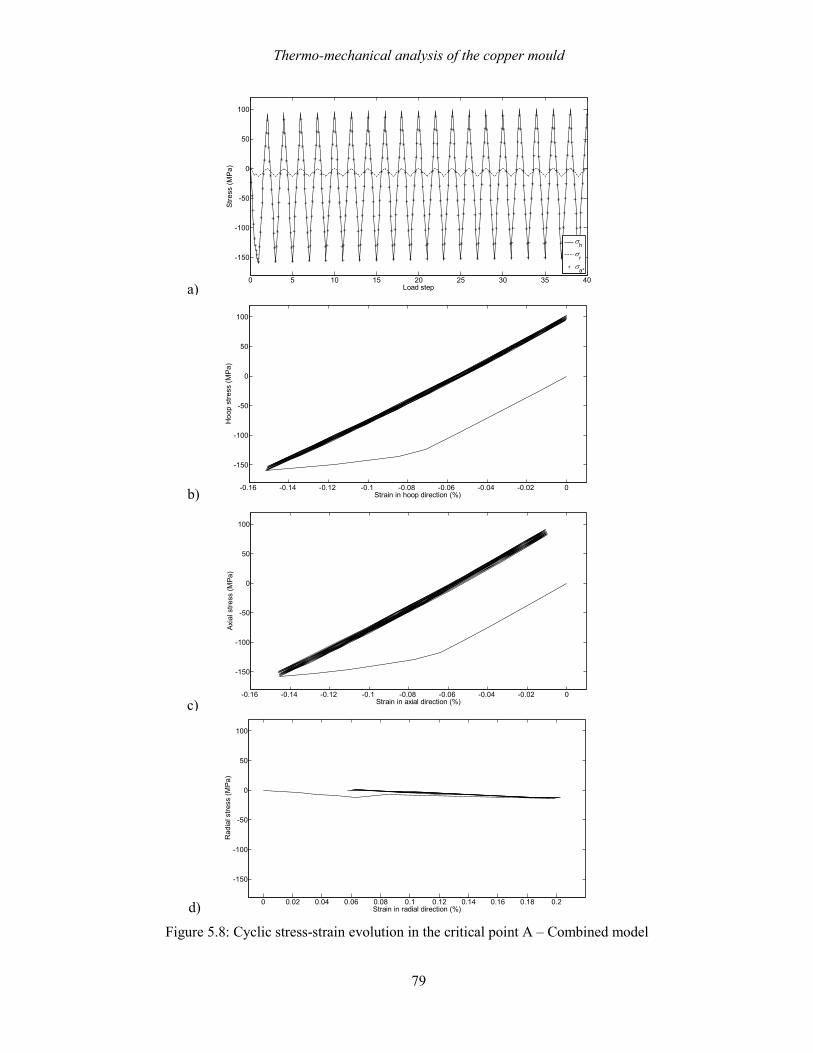
Thermo-mechanical analysis of the copper mould
79
Figure 5.8: Cyclic stress-strain evolution in the critical point A – Combined model
0 5 10 15 20 25 30 35 40
-150
-100
-50
0
50
100
Load step
Stre
ss (M
Pa)
σhσrσa*
-0.16 -0.14 -0.12 -0.1 -0.08 -0.06 -0.04 -0.02 0
-150
-100
-50
0
50
100
Strain in hoop direction (%)
Hoo
p st
ress
(MPa
)
-0.16 -0.14 -0.12 -0.1 -0.08 -0.06 -0.04 -0.02 0
-150
-100
-50
0
50
100
Strain in axial direction (%)
Axia
l stre
ss (M
Pa)
0 0.02 0.04 0.06 0.08 0.1 0.12 0.14 0.16 0.18 0.2
-150
-100
-50
0
50
100
Strain in radial direction (%)
Rad
ial s
tress
(MPa
)
a)
b)
c)
d)

Thermo-mechanical analysis of the copper mould
80
5.2.1 Comparison of different material models
Four different material models are considered and compared in this section:
Model 1 Model 2 Model 3 Model 4
Linear kinematic model Combined model
(Armstrong & Frederick’s + nonlinear isotropic)
Stabilized model Accelerated model
Table 5.1 shows parameters for the linear kinematic – Prager’s model where Clin is the initial hardening
modulus calculated from tensile tests of CuAg alloy at three temperature levels.
Table 5.1: Linear kinematic material parameters used in the numerical simulation
Temp. Clin (MPa)
20 oC 37439
250 oC 18039
300 oC 18466
Approximate number of cycles needed to reach the stabilized condition can be calculated using the
relation 2bNΔεpl ≈ 5 proposed in [Chaboche, 1986b]. The relation states that a value near 5 is a good
saturation criterion. Simulating around 60 567 cycles would be necessary to reach a stabilized stress-strain
cycle considering the critical point A and adopting the combined material model, for Δεpl=1.06x10⁻⁵
calculated by FEM and b=3.894. Simulation of such huge number of cycles requires unfeasible
computational effort and time (≈ 630 days). For this reason some alternative models as the accelerated
model described in paragraph 3.5.4 and the stabilized model described in paragraph 3.5.5 will be used for
simulations of the copper mould. The accelerated material model takes the rapidity of stabilization into
consideration. By increasing the coefficient b, the stabilized stress-stain cycle is possible to reach with
smaller number of cycles. As can be seen in Figure 5.9, the stabilization is reached within 20 cycles with
b=100.

Thermo-mechanical analysis of the copper mould
81
Figure 5.9: Number of cycles to stabilization versus speed of stabilization
Instead, the stabilized material model is considered to be when R reaches R∞. Material parameters C and γ
used in stabilized model are the same as for the Armstrong & Frederick’s model. However in this case, the
parameters E1 and σ0 are replaced with Es and σ0*, which correspond to the stabilized cycle.
The linear kinematic model is not able to simulate cyclic softening; however, it can give roughly overview
of component behaviour under thermo-mechanical loading. Moreover, estimation procedure of parameters
for the linear kinematic model is simply and does not require a lot of time to obtained necessary parameter
Et. Figure 5.10 shows only ˝hoop˝ stress-strain evolution considering different material models, since
similar trend can be obtained considering ˝axial˝ stresses and strains.
Compressive stresses appear as the temperature of the component increases in the first cycle because the
lateral thermal expansion is constrained. The component starts to plastically deform once developed
compressive stresses exceed the yield stress. Using the stabilized material model, yielding occurs at lower
stress in the first cycle, consequently, model overestimates the plasticization phenomena already in the
first cycle. Tensile stresses appear during the cooling phase. Depending on the type of the material model,
elastic or elasto-plastic behaviour is observed in successive cycles. For example, the combined material
model shows a predominant elastic behaviour. Consequently, the nonlinear isotropic softening material
model, which is dependent on plastic strain, has slight influence on behaviour of the combined model.
Therefore, a huge number of cycles have to be simulated to reach the stabilized stress-strain state. The
stabilized model instead shows an elasto-plastic behaviour. The accelerated model with imposed b=100
has reached the stabilized stress-strain cycle within 20 cycles, proofing that it is suitable to use for design
purposes.
60567
N
b
Combined model
20
≈ 3 100
Accelerated model
N=100 (≈25 hours)
UNFEASIBLE
Δεpl
NO
T R
EA
LIS
TIC
50

Thermo-mechanical analysis of the copper mould
82
Figure 5.10: Cyclic “hoop” stress-strain evolution considering different material models
-0.16 -0.14 -0.12 -0.1 -0.08 -0.06 -0.04 -0.02 0-150
-100
-50
0
50
100
Strain in hoop direction (%)
Hoo
p s
tress
(MP
a)
Linear Model
a)
-0.16 -0.14 -0.12 -0.1 -0.08 -0.06 -0.04 -0.02 0-150
-100
-50
0
50
100
Strain in hoop direction (%)
Hoo
p s
tress
(MP
a)
Stabilized Model
b)
-0.16 -0.14 -0.12 -0.1 -0.08 -0.06 -0.04 -0.02 0-150
-100
-50
0
50
100
Strain in hoop direction (%)
Hoo
p s
tress
(MPa
)
Combined Model
c)
-0.16 -0.14 -0.12 -0.1 -0.08 -0.06 -0.04 -0.02 0-150
-100
-50
0
50
100
Strain in hoop direction (%)
Hoo
p s
tress
(MPa
)
Accelerated Model
d)

Thermo-mechanical analysis of the copper mould
83
5.2.2 Accelerated material model - influence of b parameter
In the previous paragraph, it has been shown that the combined material model requires around 60 567
cycles (≈ 630 days of computation) to reach the stabilized condition. However, simulating such huge
number of cycles requires unfeasible computational effort and time. Therefore, as an alternative model has
been proposed to use the accelerated model by [Chaboche, 1986b]. Since the accelerated model takes into
consideration the speed of stabilization, the stabilized cycle is possible to reach simulating less number of
cycles by increasing b parameter.
The sensitivity analyses are performed considering the b parameter. The goal of the sensitivity analyses is
to investigate response of the model considering various values of b. The mechanical analyses are
performed with the same material parameters as for the combined material model except b for which 6
different values are considered 400, 350, 300, 200, 100, 50, respectively. “Hoop” stress-strain evolution
for the critical point A (explained at the beginning of section 5.2) and for 20 cycles are plotted in Figure
5.11. Number of 20 cycles is chosen to perform complete analysis within reasonable time (≈5 hours).
Figure 5.11: Cyclic “hoop” stress-strain evolution considering the accelerated model with different values of b
-0.2 -0.18 -0.16 -0.14 -0.12 -0.1 -0.08 -0.06 -0.04 -0.02 0-150
-100
-50
0
50
100
Strain in hoop direction (%)
Hoo
p s
tress
(MPa
)
b=400-0.2 -0.18 -0.16 -0.14 -0.12 -0.1 -0.08 -0.06 -0.04 -0.02 0
-150
-100
-50
0
50
100
Strain in hoop direction (%)
Hoo
p s
tress
(MP
a)
b=350
-0.2 -0.18 -0.16 -0.14 -0.12 -0.1 -0.08 -0.06 -0.04 -0.02 0-150
-100
-50
0
50
100
Strain in hoop direction (%)
Hoo
p s
tress
(MPa
)
b=300
-0.2 -0.18 -0.16 -0.14 -0.12 -0.1 -0.08 -0.06 -0.04 -0.02 0-150
-100
-50
0
50
100
Strain in hoop direction (%)
Hoo
p s
tress
(MP
a)
b=200
-0.2 -0.18 -0.16 -0.14 -0.12 -0.1 -0.08 -0.06 -0.04 -0.02 0-150
-100
-50
0
50
100
Strain in hoop direction (%)
Hoo
p s
tress
(MP
a)
b=100-0.2 -0.18 -0.16 -0.14 -0.12 -0.1 -0.08 -0.06 -0.04 -0.02 0
-150
-100
-50
0
50
100
Strain in hoop direction (%)
Hoo
p s
tress
(MPa
)
b=50
a) b)
c) d)
e) f)

Thermo-mechanical analysis of the copper mould
84
5.3 Metallurgical analysis of the copper mould
In the continuous casting process, the molten steel flows from the upper to the bottom part of the
mould where the cast strand exits with thin solidified shell, see Figure 5.2. The inner surface of the mould
is often plated with chromium or nickel to provide a harder working surface [Barella, 2014]. During the
solidification of steel, the huge thermal flux, q, passes from the molten steel to the inner surface of the
mould, which is then subjected to high temperatures. As consequences the high thermal gradient takes
place across plates and cause creating of thermal cracks at the inner surface in the area near meniscus
[Park, 2002b].
Figure 5.12: Copper mould under investigation
The metallurgical analysis has been carried out to determine failure and damages which had been occurred
on the copper mould. So far, similar studies have been performed by [Barella, 2014, Park, 2002b].
Metallographic and SEM (scanning electron microscope) analyses have been performed to characterize
the mould microstructure. Figure 5.12: shows the mould under investigation. Firstly, the mould was
examined visually and cut in half over the length. The inner surface of the mould after severs sequences of
production is presented in Figure 5.13. A closer examination of the mould inner surface shows that cracks
are formed in the region near the meniscus. The most damaged area is approximately 130 mm from the
mould top, i.e. in the level where the maximum temperature occurs
Figure 5.13: Closed view of the mould inner surface near the level of meniscus
100
mm
level of meniscus

Thermo-mechanical analysis of the copper mould
85
Moreover, the mould was cut into several samples to carry out SEM examination of the damaged and
undamaged areas. As can be seen in Figure 5.14, overall 14 samples were cut at different positions of
interest. Samples were named as A01, A02, A03, A04 (samples taken from corners in the level of
meniscus), A1, A1_1, A1_2, A2, A3, A4 (samples taken from walls in the level of meniscus), B1, C1, D1
and E1. All samples were grinded and polished, while etching was performed with solution H2O : NH3:
H2O2 = 1:1:1.
Figure 5.14: Schematic positions of 14 specimens
The mould microstructure has been analysed after application of etching, both on the undamaged and
damaged zones. As can be seen in Figure 5.15, many cracks were observed on the following samples A1,
A1_1, A1_2, A3, and A4 cut from walls in the level of meniscus where also the maximum temperature
occurs. The analysis showed that cracks initiate at the surface and then propagate into thickness.
Furthermore, cracks are transgranular confirming that they occurred under effect of thermal fatigue. The
microstructure, in some regions near cracks, seemed to have undergone a recrystallization process because
of the small grain size (e.g. A1_2, A3). It is observed that cracks appeared near the surface of the mould
1000
130
65
8643
195
250
250
A A
A-A
129
87
A1
A2
A3A4
A1_1 A1_2A01 A02
A03A04B1
A1
C1
D1
E1
A1_1 A1_2
A01 A02

Thermo-mechanical analysis of the copper mould
86
on the places where Cr-layer is absent. The Cr-layer was delaminated by the differential thermal
expansion between the coating and the underneath Ni layer. The grain size of the Cu is coarse and in the
range of ~70±30 µm. These dimensions are in the range of the microstructural requirements for this kind
of application (i.e. mould used for continuous casting of steel). In particular the requirements are related to
creep resistance of material that, in some areas, is working in the range of diffusional creep.
A1, 55±23µm A1_1, 87±27µm
A1_2, 55±16µm A2, 88±37µm
A3, 76±24µm A4, 82±23µm
Figure 5.15: Microstructure of samples taken from walls in the level of meniscus

Thermo-mechanical analysis of the copper mould
87
Figure 5.16: Optical micrograph of the cross section of mould cracks
No visible cracks were found during examination of samples A01 and A02, while samples A03 and A04
have few small cracks, see Figure 5.17.
A01, 50±20µm A02, 87±
A03, 75±25µm A04, 56±24µm
Figure 5.17: Microstructure of samples taken from corners in the meniscus level
Specimen: A1_2
Specimen: A3 200 µm
200 µm

Thermo-mechanical analysis of the copper mould
88
The following samples B1, C1, D1 and E1 do not have visible cracks. The chromium coating layer is
present on B1, C1, D1 and E1 specimens with thickness of approximately 100 µm.
B1, 94±23µm C1, 78±26µm
D1, 94±33µm E1, 91±29µm
Figure 5.18: Microstructure of samples B1, C1, D1 and E1
Inside the cracks were present some deposits that could not be identified by the light microscope analyses.
Therefore, the SEM investigation has been performed in order to understand the origin of these deposits.
The SEM analysis has been performed on the A1 specimen.
Figure 5.20 and Figure 5.21 show that except zinc many other residual impurities were detected in the
crack due to liquid steel infiltration Pb, Zn, S, Mn etc, see Table 5.2. Moreover, Table 5.2 shows chemical
composition observed in the undamaged zone (Figure 5.19) where small pits correspond to the region rich
of Ag precipitates.
Figure 5.19: X-ray spectrum of the undamaged zone – Spectrum 1

Thermo-mechanical analysis of the copper mould
89
Figure 5.20: X-ray spectrum of the damaged zone (crack) - Spectrum 2
Figure 5.21: X-ray spectrum of the damaged zone (crack) – Spectrum 3
Table 5.2: SEM characterization with respect to Figure 5.19, Figure 5.20 and Figure 5.21
Spectrum C O Ag S Cl Mn Fe Cu Zn Pb Total
Spectrum 1 0.55 99.45 100.0
Spectrum 2 24.61 13.84 1.34 1.99 1.67 6.10 7.25 43.21 100.0
Spectrum 3 34.49 15.59 1.97 5.15 2.33 7.08 20.13 13.26 100.0
In particular, it could be seen that the Cu substrate, when it is exposed to the molten steel, is reacting with
Zn and producing an alloyed layer that corresponds with a brittle γ phase, see Figure 5.22. This brittle
phase is enhancing the production of cracks that are propagating in the underneath Cu substrate. The
propagation is enhanced by the permeation of the low melting point of elements (Sn, Pb, Zn etc.) that are
embrittling the crack root. In this case the energy required for the crack propagation is lower than the
required for the crack propagation in bare Cu.

Thermo-mechanical analysis of the copper mould
90
Figure 5.22: SEM investigation of the undamaged zone
Table 5.3: SEM characterization with respect to Figure 5.22
Spectrum C O Si S Ca Mn Fe Cu Zn Pb Total
Spectrum 1 3.42 1.01 95.57 100.00
Spectrum 2 14.37 18.01 35.93 31.69 100.00
Spectrum 3 27.97 18.06 0.42 2.14 0.34 5.16 3.74 3.17 29.25 9.76 100.00
Chapter 5 has presented results obtained with the thermo-mechanical analysis where as a study case a
copper mould was taken into consideration. The thermo-mechanical analysis have been performed with
respect to several material models (the combined model, the linear kinematic, the stabilized and the
accelerated model) to investigate influence of a material model on cyclic stress-strain response in a
component. Results, i.e. stress-strain responses, obtained with different models will be used as a base to
calculate the service life of analysed component in Chapter 6.

Fatigue life assessment
91
Chapter 6
Fatigue life assessment
Fatigue damages which occur due to thermo-mechanical cyclic loads distinguishes from damages
occur due to temperature variation [Halford, 1986, Halford, 1987]. Prediction of a thermo-mechanical
fatigue life based on thermal fatigue data is not simple. The most accurate way to assess a fatigue life is to
establish its behaviour by actual experiment. However, in most cases conducting an extensive
experimental test, especially at beginning of research, cannot be performed. Several models have been
developed and proposed in [Manson, 1966, Manson, 1967, Manson, 2006], to preliminary assess a fatigue
life without involving prior knowledge of fatigue behaviour. Some of these methods are based on
monotonic uniaxial test properties of material under investigation. More discussion is given in Chapter 6
regarding these models.
Generally, fatigue in terms of number of cycles is divided into two specified parts; low and high cycle
fatigue. Low cycle fatigue (LCF) occurs when during the cyclic loading the plastic deformation is
dominant; the strain-life approach is suggested to be used in this situation. High cycle fatigue (HCF)
occurs when the stresses are low enough that the strains are elastic. Stress-based approach is suggested to
be used in the case of HCF. Strain or stress based approaches allow engineering designer to assess the
fatigue life of a component. The strain-based fatigue approaches are considered in Chapter 6.
First few paragraphs of Chapter 6 are focused on strain-based fatigue models (Manson-Coffin-
Basquin). Moreover, the particular attention is given to alternative models whose parameters can be
estimated using simple tensile test data (Universal Slopes equation, Modified Universal Slopes equation).
Identification procedure of the Manson-Coffin-Basquin as well as of alternative models (Universal Slopes
equation, Modified Universal Slopes equation) is described afterwards. The experimental data are
invariably scattered, since test specimens and testing conditions are never identical. Therefore, statistical
methods have been used to analysis the fatigue test data. The last part of Chapter 6 is focused to various
models (deterministic and probabilistic) suitable to define design curves. The design curve is established

Fatigue life assessment
92
by adopting characteristic value (probability of failure) that lay a certain number of standard deviation
below the mean ε-N curve. The last part deals with the fatigue life assessment of a component subjected to
thermo-mechanical cyclic loading. For this purpose, the copper mould used in the continuous casting
process of steel is considered as an example.
6.1 Stress-based approach
Fatigue started to be investigated in the middle of the nineteenth century when the fatigue failures of
railway axes became a widespread problem. The German engineer August Wöhler set up and carried out
the first systematic fatigue investigation. August Wöhler investigated the progressive failure of railway
axles which had failed after various time in service, at loads considerable less than expected. Wöhler
studies resulted in development of the stress-based approach. The stress-based approach is the oldest
method used in the fatigue design and it is also referred to as the S-N (stress versus number of cycles to
failure) approach [Lee, 2005, Stephens, 2001]. The S-N approach is distinguished from the other fatigue
models by several features: cyclic stresses are the governing parameters for fatigue failure and high-cycle
fatigue conditions. To develop the S-N diagram, a series of samples are tested at various stress ranges and
several samples are tested at each stress range. Generally, S-N diagrams are plotted in log-log scale, where
the stress amplitude is plotted on the vertical axis and cycles to failure on the horizontal axis, see Figure
6.1. In 1910, Basquin proposed following relationship between stress amplitude and lifetime:
( ) *
ffa 2' bNσσ = 6.1
where σf' is the fatigue strength coefficient, b* is fatigue strength exponent also known as Basquin
exponent and 2Nf is reversals to failure (1 reversal=1/2 cycle). Basquin equation is rewritten in terms of
strain based approach in paragraph 6.3. When the stress on a particular region of a material varies
sinusoidally from tension to compression and back again is known as fully reversed loading. Fully
reversed indicates that loading is alternating about a zero mean stress (σm). As can be seen in Figure 6.2,
the stress range (Δσ), the stress amplitude (σa) and the mean stress are parameters which characterize a
cyclic loading and can be expressed as:
max min max minmax min a m, , =
2 2σ σ σ σσ σ σ σ σ− +
∆ = − = 6.2
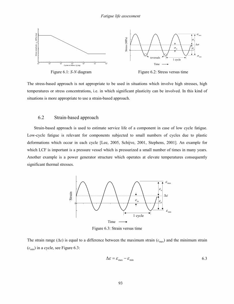
Fatigue life assessment
93
Figure 6.1: S-N diagram Figure 6.2: Stress versus time
The stress-based approach is not appropriate to be used in situations which involve high stresses, high
temperatures or stress concentrations, i.e. in which significant plasticity can be involved. In this kind of
situations is more appropriate to use a strain-based approach.
6.2 Strain-based approach
Strain-based approach is used to estimate service life of a component in case of low cycle fatigue.
Low-cycle fatigue is relevant for components subjected to small numbers of cycles due to plastic
deformations which occur in each cycle [Lee, 2005, Schijve, 2001, Stephens, 2001]. An example for
which LCF is important is a pressure vessel which is pressurized a small number of times in many years.
Another example is a power generator structure which operates at elevate temperatures consequently
significant thermal stresses.
Figure 6.3: Strain versus time
The strain range (Δε) is equal to a difference between the maximum strain (εmax) and the minimum strain
(εmin) in a cycle, see Figure 6.3:
max minε ε ε∆ = − 6.3
102 103 104 105 106 107 108
Cycles to failure, Nf (log)
Stre
ss a
mpl
itude
, σa (
MP
a) (l
og)
maxσ
minσ
σ∆aσ
aσmσ
Stre
ss (M
Pa)
reversals 1 cycle
Time
maxε
minε
ε∆aε
aεmεStra
in
1 cycle Time
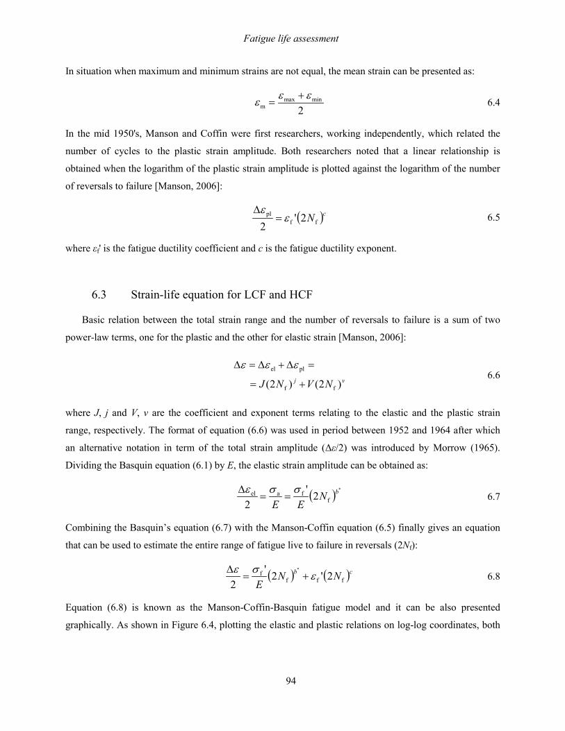
Fatigue life assessment
94
In situation when maximum and minimum strains are not equal, the mean strain can be presented as:
max minm 2
ε εε +=
6.4
In the mid 1950's, Manson and Coffin were first researchers, working independently, which related the
number of cycles to the plastic strain amplitude. Both researchers noted that a linear relationship is
obtained when the logarithm of the plastic strain amplitude is plotted against the logarithm of the number
of reversals to failure [Manson, 2006]:
( )cNffpl 2'
2ε
ε=
∆ 6.5
where εf' is the fatigue ductility coefficient and c is the fatigue ductility exponent.
6.3 Strain-life equation for LCF and HCF
Basic relation between the total strain range and the number of reversals to failure is a sum of two
power-law terms, one for the plastic and the other for elastic strain [Manson, 2006]:
vj NVNJ )2()2( ff
plel
+=
=∆+∆=∆ εεε 6.6
where J, j and V, v are the coefficient and exponent terms relating to the elastic and the plastic strain
range, respectively. The format of equation (6.6) was used in period between 1952 and 1964 after which
an alternative notation in term of the total strain amplitude (Δε/2) was introduced by Morrow (1965).
Dividing the Basquin equation (6.1) by E, the elastic strain amplitude can be obtained as:
( ) *
ffael 2'
2bN
EEσσε
==∆
6.7
Combining the Basquin’s equation (6.7) with the Manson-Coffin equation (6.5) finally gives an equation
that can be used to estimate the entire range of fatigue live to failure in reversals (2Nf):
( ) ( )cb NNE fff
f 2'2'2
*
εσε+=
∆ 6.8
Equation (6.8) is known as the Manson-Coffin-Basquin fatigue model and it can be also presented
graphically. As shown in Figure 6.4, plotting the elastic and plastic relations on log-log coordinates, both

Fatigue life assessment
95
curves become straight lines. Superposition of the elastic and the plastic components gives the fatigue life
in terms of total strain.
Figure 6.4: Manson-Coffin-Basquin strain life curve
Transition fatigue life (point T in Figure 6.4) is obtained by intersection of the elastic and the plastic strain
lines. Transition fatigue life presents the fatigue life at which the elastic strain amplitude and the plastic
strain amplitude are equal, see Figure 6.4. Equation for the transition fatigue life (2Nt) can be derived by
equations (6.5) and (6.7):
( )cb
EN−
=
*1
f
ft '
'2σε
6.9
Region in which the plastic deformation is dominant, left of the transition point, is referred to as the low
cycle fatigue (LCF) region. The high-cycle fatigue (HCF) region, in which the elastic strain is dominant, is
placed right regarding the transition point.
6.4 The Universal Slopes equation
Often fatigue life of a component with a reasonable degree of accuracy is desirable to estimate using
some simpler approach. For example, fatigue test data is required to estimate four Manson-Coffin-Basquin
parameters. Conduction of fatigue tests can be more time-consuming and expensive in comparison with
monotonic tension tests. This leads to development of several methods which correlate monotonic strength
and fatigue life. Basic material properties such as the Young’s modulus, the ultimate tensile strength and
the ductility can be obtained from monotonic tension test. It is important to note that the stress-strain
Reversal to failure, 2Nf (log scale)
Stra
in a
mpl
itude
, εa
(log
scal
e)
b*
c
T
el
2ε∆
pl
2ε∆ plel
2 2 2εε ε ∆∆ ∆
= +
Total strain amplitude
Elastic component
Plastic component
Transition point
fε ′
f
Eσ ′
Reversals to failure, 2Nf (log scale)
Stra
in a
mpl
itude
, εa
(log
scal
e)
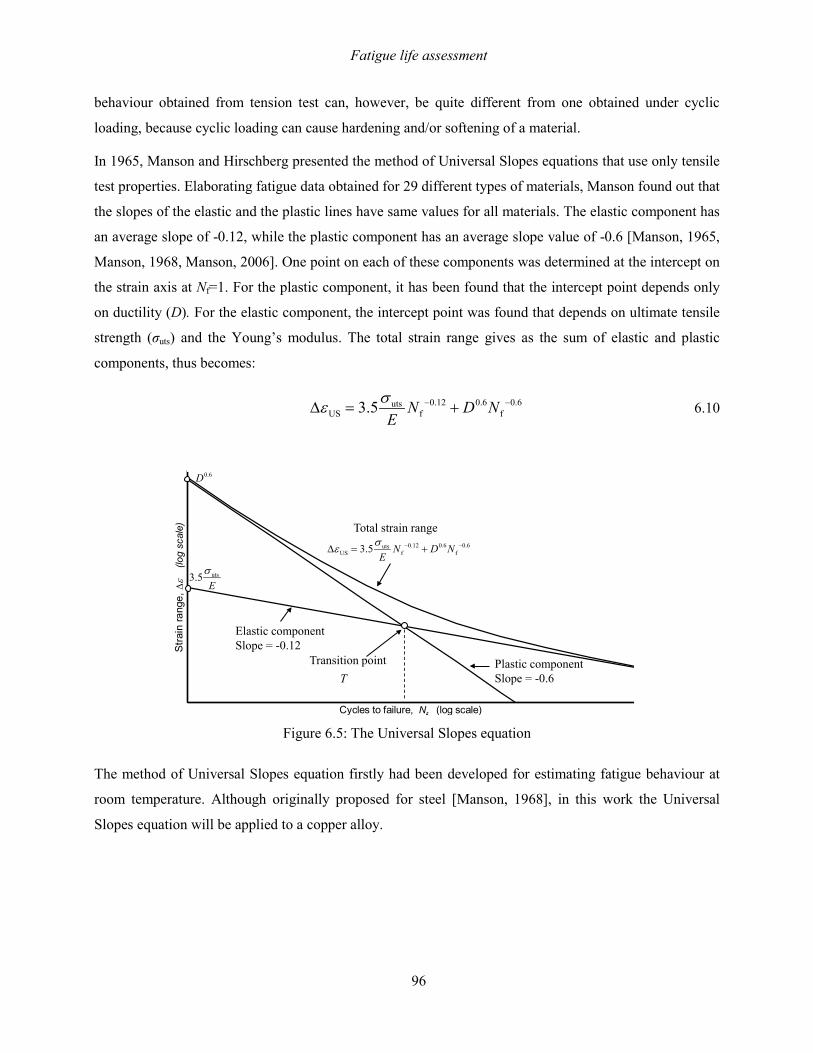
Fatigue life assessment
96
behaviour obtained from tension test can, however, be quite different from one obtained under cyclic
loading, because cyclic loading can cause hardening and/or softening of a material.
In 1965, Manson and Hirschberg presented the method of Universal Slopes equations that use only tensile
test properties. Elaborating fatigue data obtained for 29 different types of materials, Manson found out that
the slopes of the elastic and the plastic lines have same values for all materials. The elastic component has
an average slope of -0.12, while the plastic component has an average slope value of -0.6 [Manson, 1965,
Manson, 1968, Manson, 2006]. One point on each of these components was determined at the intercept on
the strain axis at Nf=1. For the plastic component, it has been found that the intercept point depends only
on ductility (D). For the elastic component, the intercept point was found that depends on ultimate tensile
strength (σuts) and the Young’s modulus. The total strain range gives as the sum of elastic and plastic
components, thus becomes:
0.12 0.6 0.6utsUS f f3.5 N D N
Eσε − −∆ = +
6.10
Figure 6.5: The Universal Slopes equation
The method of Universal Slopes equation firstly had been developed for estimating fatigue behaviour at
room temperature. Although originally proposed for steel [Manson, 1968], in this work the Universal
Slopes equation will be applied to a copper alloy.
Cycles to failure, Nf (log scale)
Stra
in ra
nge,
∆ε
(lo
g sc
ale)
T
0.12 0.6 0.6utsUS f f3.5 N D N
Eσε − −∆ = +
Total strain range
Elastic component Slope = -0.12
Plastic component Slope = -0.6
Transition point
0.6D
uts3.5Eσ

Fatigue life assessment
97
6.5 10% and 20% Rule
Next attempt was to apply the Universal Slopes equation using the tensile properties at high
temperature of interest. The fatigue life for a given strain range at high temperature may be expected to be
lower than that for the same strain range at a temperature below half the melting point. Creep, oxidation
and high temperatures are known to reduce up to 90% of fatigue life. A rough estimate is provided by
10% Rule as suggested in [Manson, 1967, Manson, 1968, Manson, 2006, Manson, 2009]. The 10% Rule
estimates that, at the high temperatures, only 10% of the life computed by the Universal Slopes equation
will actually be achieved. The Universal Slopes equation gives the upper bound life, while the 10% Rule
gives the lowest expected life i.e. lower bound life.
Median expected life is estimated to be 2 times of the lowest bound life [Manson, 2009]. The 20% Rule
assumes that, at the high temperatures, only 20% of the life computed by the Universal Slopes equation
will actually be achieved. Since as suggested [Manson, 1968] an average mean fatigue life has been
estimated to be twice of the lower bound (20%).
Figure 6.6: 10% and 20% Rule
Cycles to failure, Nf (log scale)
Stra
in ra
nge,
∆ε
(lo
g sc
ale)
%10ε∆
USε∆
%20ε∆
Universal Slopes equation
20% Rule
10% Rule

Fatigue life assessment
98
6.6 The Modified Universal Slopes equation
In 1986, Muralidharan and Manson conducted a study on 50 different materials with the intention to
re-exanimate and to improve the Universal Slopes equation accuracy. The Universal Slopes equation
(6.10) was further modified to the following expression [Manson, 2006, Pope, 1997]:
0.832 0.53
0.09 0.155 0.56uts utsMUS f f1.17 0.0266N D N
E Eσ σε
−− − ∆ = +
6.11
In the first term, representing the elastic component, slope has become -0.09 instead of -0.12. Lower value
(-0.09) contributes that the elastic line calculated by equation (6.11) is shifted above regarding the elastic
line calculated by equation (6.10), see Figure 6.7. In the second term, representing the plastic component,
new exponent -0.56 differs little from the original value of -0.6; but instead of involving only a ductility
term, the new equation contains both the strength term [≈(σuts/E)1/2] and the ductility term with a
considerable lower exponent [Manson, 2006]. As can be seen in Figure 6.7, the plastic line calculated by
equation (6.11) is shifted above the plastic line calculated by equation (6.10). Finally, the curve ΔεMUS,
which is the sum of the elastic and plastic components, is thus displaced slightly upward regarding
Universal Slopes Equation obtained with parameters from tensile test data at 250 oC. The displacement is
the greatest in the region of HCF where the elastic component predominates. The equation (6.11) should
be used only in the sub-creep temperature range (up to about half of the absolute melting temperature of a
material). Furthermore, the ductility and the ultimate strength used in equation should be estimated at a
temperature for which the fatigue life is calculated [Edward, 1997].
Figure 6.7: Comparison between Universal Slopes and Modified Universal Slopes equations
Cycles to failure, Nf (log scale)
Stra
in ra
nge,
∆ε
(lo
g sc
ale)
Universal Slopes equation (250 oC)Modified Universal Slopes
Total strain ranges
Elastic components
Plastic components

Fatigue life assessment
99
6.7 Statistical aspects of fatigue
Generally, fatigue experimental data are subjected to considerable scatter. Statistical analyses are used
to describe and to analyse fatigue properties as well as to determine the probability associated with fatigue
life of a component. Some basic concepts commonly adopted for the statistic characterization of fatigue
data is given hereafter. Figure 6.8 illustrates the statistical scatter typical for fatigue data. Plenty of factors
contribute to scatter:
• production and surface quality of a specimen,
• accuracy of test equipment as well as skill of laboratory technicians,
• environment in a laboratory (controlled temperature and humidity) etc.
Figure 6.8: Schematically description of a strain-based fatigue curve
A quantity such as the fatigue data has a statistical variation called ˝stochastic variable˝, X. Characteristics
of a variable for a population are usually obtained from a small part of the population, called a sample
[Stephens, 2001]. The mean or average for a sample size n is defined as:
∑=
=n
iiX
nX
1
1 6.12
Here, Xi denotes a random variable such as the plastic strain amplitude in the strain-life fatigue test. The
mean value gives a measure of the central value of the sample. Dispersion of values in the sample is
measured by the sample standard deviation [Stephens, 2001]:
( )( )1
1
2
−
−=∑=
n
XXS
n
ii
6.13
Median (50%)
Design curve
pdf of 2Nf given εa
fatigue data
εa(log)
2Nf (log)

Fatigue life assessment
100
Standard deviation gives a measure of the magnitude of the variation. Parameter which is widely used to
describe the uncertainty is the coefficient of variation, C, which is given by:
XSC = 6.14
Fatigue data have significant scatter which can be described by the probability density function (pdf) as
shown in Figure 6.8. Generally, statistical models are employed to describe the distribution of the
observed factor. For instance, the random variable Nf is usually described with 2-parameter Weibull or
normal model.
6.7.1 Linear model
The scatter diagram, presented in Figure 6.9, shows the plastic strain amplitude versus the number of
reversal to failure plotted on a log-log diagram. It can be noticed that there is a strong indication that
points (e.g. experimental data) lie scattered randomly around a straight line.
Figure 6.9: Scatter diagram of a fatigue data
Identification of a straight line can be done by adopting a simple linear model [Martinez, 2002, Marques,
2007, Montgomery, 2003, Stephens, 2001]:
Y A BX= + 6.15
in which X is a single independent or controlled variable and Y is a dependent variable, the relation is
usually denoted as YǀX. In case of Manson-Coffin equation (6.5), Y=log(εpl,a) and X=log(2Nf). The
intercept (A) and slope (B) are unknown regression coefficients. More appropriate way to solve this
problem takes into consideration also the normal distributed random variable error, ε:
εY A BX= + + 6.16
εpl,a(log)
2Nf (log)

Fatigue life assessment
101
where the error has mean zero and variance S2 which is unknown. Taking into account the error
variability, Y is also a random variable. Using equation (6.16), it is possible to express the n observations
in the sample as:
iii BXAY ε++= , i=1, 2,…,n 6.17
The least squares estimates of the slope and intercept in the simple linear regression model are:
( ) ( )
( )1
2
1
ˆ
n
i ii
n
ii
X X Y YB
X X
=
=
− −=
−
∑
∑ 6.18
ˆ ˆA Y BX= − 6.19
where Â, B̂ are least squares estimators and X̅, Y̅ are the average values of X and Y:
∑ ∑= =
==n
i
n
iii X
nXY
nY
1 1 1 , 1 6.20
The fitted or estimated regression line has the following form:
ˆˆ ˆY A BX= + 6.21
Noting that each pair of observations satisfies the relationship:
iii XBAY eˆˆ ++= , i=1,2…,n 6.22
where ei is the residual expressed as:
iii YY ˆe −= 6.23
The residuals describe the error in the fit of the model to the ith observation Yi. The sum of squared errors
is defined as:
∑∑==
−==n
iii
n
ii YYSSE
1
2
1
2 )ˆ(e 6.24
The sum of squares due to regression is expressed as:
∑=
−=n
iii YYSSR
1
2)ˆ( 6.25
While the total sum of squares is:
∑=
−=n
iii YYSST
1
2)( 6.26

Fatigue life assessment
102
R-squared (R2) is the statistic measure which shows how close the data are to the fitter regression line, it is
also known as the coefficient of determination.
SSTSSE
SSTSSRR −== 12 6.27
In general, R2 is always between 0 and 1.0. The higher the R2 is, the model better fits to the data. In the
Chapter 4, the SSE as well as R2 have been used to provide information about adequacy of the fitted
model.
Figure 6.10: Schematically representation of SSE, SSR and SST
6.8 Identification procedure of fatigue life parameters
The identification procedure of Manson-Coffin-Basquin parameters is described in this paragraph.
Parameters are estimated using low cycle fatigue experimental data of a CuAg alloy at three temperature
levels (20 oC, 250 oC and 300 oC). Afterwards, three main parameters that define the Universal Slopes
equation and Modified Universal Slopes equation are estimated using tensile test data of a CuAg alloy
performed at 20 oC, 250 oC and 300 oC.
6.8.1 Manson-Coffin-Basquin parameters
Several low cycle fatigue tests with a load ration Rε=-1 at different strain ranges are necessary to
perform to identify four Manson-Coffin-Basquin parameters. In general, fatigue tests are expensive, time-
consuming and therefore often large sizes of samples are not possible. Sufficient numbers of specimens
are important to test in order to obtain statistical meaningful results due to a considerable amount of
scattering which appears in fatigue test data. Parameters uncertainty is relatively large in case of small
number of samples.
Y
X

Fatigue life assessment
103
Four Manson-Coffin-Basquin parameters are estimated separately by performing linear regression
analysis [Nieslony, 2008]. The estimated parameters are valid in the range of the experimental data.
Linearization of the Manson-Coffin equation (6.5) leads to:
( ) cXY += 'log fε 6.28
where
( ) ( )pl,a flog , log 2Y X Nε= =
6.29
the fatigue ductility parameter (εf') and the ductility exponent, (c), are the intercept and the slope,
respectively, of the linear least square fit to the plastic strain amplitude versus the reversals to failure,
using a log-log scale. Next step is to apply the least-squares method using equations 6.13, 6.18 and 6.19 to
estimate S, �̂�𝐴 and 𝐵𝐵� , respectively. Once all values are calculated, the Manson-Coffin parameters could be
estimated with following relations:
cA-
Bc ˆˆ
f 10'ˆ ˆ1ˆ == ε
Linearization of Basquin’s equation (6.1) gives:
XbE
Y *f 'log +
=σ
6.30
where
( ) ( )el,a flog , log 2Y X Nε= =
6.31
Similarly, the fatigue strength coefficient (σf') and the fatigue strength exponent (b*) are the intercept and
slope, respectively, of the linear least squares fit to the elastic strain amplitude versus reversals to failure,
using a log-log scale. Finally, the Basquin parameters are obtained also by applying the least squares
method and using the following relations:
*ˆˆf* 10
E'ˆ ˆ
1ˆ bA-
Bb ==
σ
Figure 6.11 shows calculated strain life curve regarding LCF experimental data for CuAg alloy performed
at 20 oC.

Fatigue life assessment
104
Figure 6.11: Strain-life curves of CuAg for T=20 oC
Manson-Coffin-Basquin parameters (σf', b*, εf', c) have been estimated with the least-squares method
explained earlier and considering LCF tests of CuAg alloy at three temperature levels (20 oC, 250 oC and
300 oC). The parameters are summarized in Table 6.1. Experimental data of 8 specimens were available
for test performed at 20 oC, while 7 specimens were tested at 250 oC and 300 oC.
Figure 6.12 and Figure 6.13 show calculated strain life curves with respect to LCF data of CuAg alloy at
250 oC and 300 oC, respectively. The parameters determined with the least-squares method are valid in the
range of the experimental data [Lee, 2005].
Figure 6.12: Strain-life curves of CuAg for T=250 oC
102 103 104 105 106 10710-4
10-3
10-2
10-1
Reversals to failure, 2Nf (log scale)
Stra
in a
mpl
itude
, ε a
(log
scal
e)
εaεpl,aεel,a
102 103 104 105 106 10710-4
10-3
10-2
10-1
Reversals to failure, 2Nf (log scale)
Stra
in a
mpl
itude
, ε a
(log
scal
e)
εaεpl,aεel,a

Fatigue life assessment
105
Figure 6.13: Strain-life curves of CuAg for T=300 oC
Determined Manson-Coffin-Basquin parameters are summarized in Table 6.1 with respect to temperature
at which tests have been performed.
Table 6.1: Estimated parameters for Manson-Coffin-Basquin method
Temperature (oC)
σf' (MPa)
b*
εf'
c
20 359.1 -0.1065 0.09485 -0.4167
250 253.6 -0.1133 0.3666 -0.5551
300 240.4 -0.1125 0.5747 -0.6035
Comparison between strain-life curves calculated with respect to CuAg alloy at different temperatures is
presented in Figure 6.14. As can be seen in Figure 6.14, the total strain-life curve for 20 oC is situated
below the total strain-life curves for 250 oC and 300 oC in the region 2Nf<104. While situation is opposite
in the region 2Nf>104, where the total strain curve for 20 oC is situated above the curves for 250 oC and
300 oC, consequently predicting the highest life for strain amplitudes below εa=0.003.
102 103 104 105 106 10710-4
10-3
10-2
10-1
Reversals to failure, 2Nf (log scale)
Stra
in a
mpl
itude
, ε a
(log
scal
e)
εaεpl,aεel,a

Fatigue life assessment
106
Figure 6.14: Temperature dependence of total strain-life curves
6.8.2 Universal Slopes parameters
Both Universal Slopes and Modified Universal Slopes equations are based on the ultimate strength
and ductility that can be determined from a tensile test. All necessary parameters (the ultimate strength,
reduction in area and ductility) are estimated from the tensile test data of CuAg alloy performed at 20oC,
250oC and 300oC. The reduction in area (%RA) is calculated using equation (2.7), where the initial cross-
section area and the area at fracture of each specimen is needed to measure. Ductility is calculated with
equation (2.8). Obtained parameters are listed in Table 6.2.
Table 6.2: Material parameters for Universal Slopes and Modified
Universal Slopes equations
Temperature (oC)
σuts (MPa)
%RA
D
20 234 78.5 1.54
250 168 64.7 1.04
300 158 64.6 1.03
102 103 104 105 106 10710-4
10-3
10-2
10-1
Reversals to failure, 2Nf (log scale)
Stra
in a
mpl
itude
, ε a
(log
scal
e)
T=20 °CT=250 °CT=300 °C

Fatigue life assessment
107
6.9 Design curves
A strain-life curve obtained using the least squares method represents median i.e. curve with 50%
probability of failure. Design curves that incorporate the safety factor to be on the safe side during the
designing process are important take into consideration. Design curves are constructed to ensure that a
major of the fatigue data falls above the minimum or lower bound value. The choice of the lower bound
strain-life curve depends upon material cost, safety policy and industrial standards. Two possible
approaches (i.e. a deterministic and a probabilistic approach) exist to incorporate fatigue experimental data
into a design procedure. [Schneider, 2003, Williams, 2003]
6.9.1 Deterministic approach
The deterministic approach considers only scatter of a material which can be described with the
variance (S2) and calculated using equation (6.13). At the same time neglecting the fact that parameters
estimated using least squares method are random variables.
The deterministic approach assumes that a design curve is established on the safe side of data. It is
possible to establish a curve below which only 10% of the points would be expected to fall by considering
that YǀX is normal with standard deviation of S. Let β denote a probability of Y (or N) being less than the
design curve for any X. The standard normal variable associated with β is denoted as zβ. The design curve
can be calculated using following expression:
SzYN β−−= 1Dˆ2log 6.32
where 2ND is the number of reversals to failure with a probability β. Obtained design curve is transferred
to the left for a value zβS in regard to the curve calculated by the least squares method as can be seen in
Figure 6.15. Figure 6.15 shows comparison between two different approaches (the least squares method
vs. deterministic approach with a probability β=10%) considering fatigue data for CuAg alloy at 20 oC.
Figure 6.15 shows elastic, plastic and total strain amplitude versus number of reversals to failure plotted
on different graphs due to better overview.
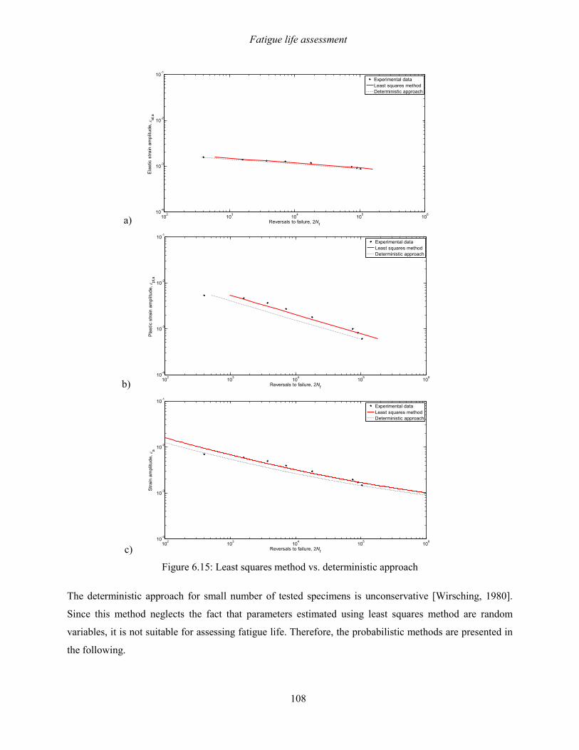
Fatigue life assessment
108
Figure 6.15: Least squares method vs. deterministic approach
The deterministic approach for small number of tested specimens is unconservative [Wirsching, 1980].
Since this method neglects the fact that parameters estimated using least squares method are random
variables, it is not suitable for assessing fatigue life. Therefore, the probabilistic methods are presented in
the following.
102 103 104 105 10610-4
10-3
10-2
10-1
Reversals to failure, 2Nf
Ela
stic
stra
in a
mpl
itude
, εel
,a
Experimental dataLeast squares methodDeterministic approach
102 103 104 105 10610-4
10-3
10-2
10-1
Reversals to failure, 2Nf
Pla
stic
stra
in a
mpl
itude
, εpl
,a
Experimental dataLeast squares methodDeterministic approach
102 103 104 105 10610-4
10-3
10-2
10-1
Reversals to failure, 2Nf
Stra
in a
mpl
itude
, εa
Experimental dataLeast squares methodDeterministic approach
a)
b)
c)
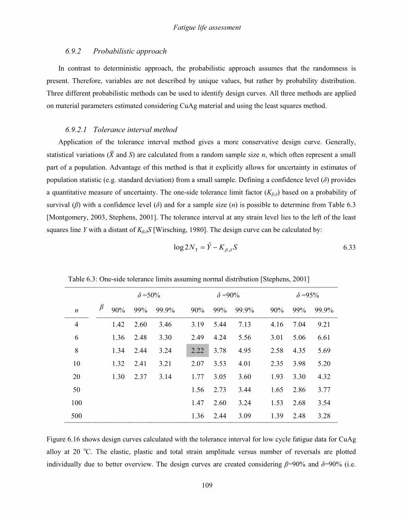
Fatigue life assessment
109
6.9.2 Probabilistic approach
In contrast to deterministic approach, the probabilistic approach assumes that the randomness is
present. Therefore, variables are not described by unique values, but rather by probability distribution.
Three different probabilistic methods can be used to identify design curves. All three methods are applied
on material parameters estimated considering CuAg material and using the least squares method.
6.9.2.1 Tolerance interval method Application of the tolerance interval method gives a more conservative design curve. Generally,
statistical variations (𝑋𝑋� and S) are calculated from a random sample size n, which often represent a small
part of a population. Advantage of this method is that it explicitly allows for uncertainty in estimates of
population statistic (e.g. standard deviation) from a small sample. Defining a confidence level (δ) provides
a quantitative measure of uncertainty. The one-side tolerance limit factor (Kβ,δ) based on a probability of
survival (β) with a confidence level (δ) and for a sample size (n) is possible to determine from Table 6.3
[Montgomery, 2003, Stephens, 2001]. The tolerance interval at any strain level lies to the left of the least
squares line Y with a distant of Kβ,δS [Wirsching, 1980]. The design curve can be calculated by:
SKYN δβ ,Tˆ2log −= 6.33
Table 6.3: One-side tolerance limits assuming normal distribution [Stephens, 2001]
δ =50% δ =90% δ =95%
n β 90% 99% 99.9% 90% 99% 99.9% 90% 99% 99.9%
4 1.42 2.60 3.46 3.19 5.44 7.13 4.16 7.04 9.21
6 1.36 2.48 3.30 2.49 4.24 5.56 3.01 5.06 6.61
8 1.34 2.44 3.24 2.22 3.78 4.95 2.58 4.35 5.69
10 1.32 2.41 3.21 2.07 3.53 4.01 2.35 3.98 5.20
20 1.30 2.37 3.14 1.77 3.05 3.60 1.93 3.30 4.32
50 1.56 2.73 3.44 1.65 2.86 3.77
100 1.47 2.60 3.24 1.53 2.68 3.54
500 1.36 2.44 3.09 1.39 2.48 3.28
Figure 6.16 shows design curves calculated with the tolerance interval for low cycle fatigue data for CuAg
alloy at 20 oC. The elastic, plastic and total strain amplitude versus number of reversals are plotted
individually due to better overview. The design curves are created considering β=90% and δ=90% (i.e.

Fatigue life assessment
110
assuming 10% probability of failure) and 8 number of tested specimens. Based on this assumption
Kβ,δ=2.22, taken from Table 6.3. Table 6.3 lists the values of the one-side factor based on normal
distribution for various sample sizes, confidence levels and probability of survival.
Figure 6.16: Least squares method vs. design curve - tolerance interval
102 103 104 105 10610-4
10-3
10-2
10-1
Reversals to failure, 2Nf
Ela
stic
stra
in a
mpl
itude
, εel
,a
Experimental dataLeast squares methodTolerance interval
102 103 104 105 10610-4
10-3
10-2
10-1
Reversals to failure, 2Nf
Pla
stic
stra
in a
mpl
itude
, εpl
,a
Experimental dataLeast squares methodTolerance interval
102 103 104 105 10610-4
10-3
10-2
10-1
Reversals to failure, 2Nf
Stra
in a
mpl
itude
, εa
Experimental dataLeast squares methodTolerance interval
a)
b)
c)

Fatigue life assessment
111
6.9.2.2 Student’s distribution - t The Student’s distribution is suggested to use in order to calculate the variability of experimental data
for small number of samples; even if phenomenon can be described with normal distribution. Student’s
distribution is symmetric [Montgomery, 2003]. The design curve can be defined considering the
probability of failure β and Student’s distribution with n-2 degrees of freedom by equation:
( )2X
2
2;1S1ˆ2log
nSXX
nnStYN n
−+
+−= −−β 6.34
where 2NS is number of reversal with a probability of failure β, t is the Student’s variate and can be find in
the statistical tables of a Student’s distribution. While
( )2
1
2X
1∑=
−=n
iXX
nS 6.35
Figure 6.17 shows comparison between design curves obtained with three different methods. Both curves,
(Student’s and deterministic) are calculated with the probability of failure 10%. As can be seen, the design
curve obtained with the Student’s distribution is the most conservative while the curve calculated with
deterministic approach is less conservative. Moreover, the Student’s curve is not a straight line but it is
slightly curved. Only the plastic strain range versus the number of reversals is plotted. However, plotting
the elastic or the total strain versus the number of reversals gives the same results. The Student’s curve can
be interpreted as follows: on the basis of the available data, there is a 10% chance that the next YǀX
selected would fall below this curve.
Figure 6.17: Least squares method vs. design curve - tolerance interval and Student’s distribution
102 103 104 105
10-3
10-2
Reversals to failure, Nf
Plas
tic s
train
, εpl
Experimental dataLeast squares methodDeterministic approachStudent distribution

Fatigue life assessment
112
Analysing the equation (6.34) can be demonstrated that for large number of samples (n→∞) it is obtained
that t1-β;n-2→z1-β and the radical term tends to 1. Therefore for a large n, equation (6.34) approaches
equation (6.32), i.e. Student’s distribution tends to the normal distribution.
6.9.2.3 Equivalent prediction interval (EPI) The equivalent prediction interval (EPI) approach is based on linearization of a curve calculated by the
Student’s distribution. It is assumed that YǀX has a normal distribution with mean to model the uncertainty
in Y [Wirsching, 1983]:
XBAY ˆˆˆ +=
and equivalent standard deviation, Se. where combination of equation (6.32) and equation (6.34) gives Se.
Moreover, S has been replaced with Se considering the equation (6.32). It is obtained:
( )
−+
+= −−− 2
X
2
2;1e11
nSXX
nntSSz nββ 6.36
Probabilities associated with the normal and Student’s are assumed to be equal. As they are two different
models, equality can exist only at one point β. Finally based on equality, the equivalent standard deviation
is defined as:
( ) ( )
−+
+=≡
−
−−2
2
1
2;1ee
1,,X
n
nSXX
nn
zt
SnXSSβ
ββ 6.37
The equivalent standard deviation, defined in the equation (6.37), seems to be quite complicate for an
engineering scope. Furthermore, Se does not assume a constant value as it depends on X, n as well as on β.
However, the standard deviation should be a constant value. This problem can be fixed introducing a new
term. As it has been already explained, the design curve calculated by the Student’s distribution becomes
flat as number of samples is equal or higher than 15 (n≥15) [Wirsching, 1980]. This characteristic gives a
possibility of simplifying the model by introducing an equivalent and constant standard deviation, So. The
equivalent constant standard deviation gives ability that these probability design curves can be
approximated as straight lines. Obtained lines are called herein as equivalent prediction intervals or
abbreviated EPI. The equivalent constant standard deviation of Y is defined as [Wirsching, 1980]:
( )β,o nSgS = 6.38
where g(n, β) is an approximation to the terms in brackets in equation (6.37) and also an adjustment factor
of the S which takes into consideration uncertainty in the estimates of �̂�𝐴, 𝐵𝐵� and S. The adjustment factor is
applied to standard deviation previously calculated with linear regression and it can be calculated as:

Fatigue life assessment
113
( ) ( ) ( ) ( ), exp ln Bg n A n ββ β − = 6.39
in which:
( ) ( )( )
1.1211.56 tanh 1
3.32 1.7
A
B
β β
β β
− = − = −
6.40
The equivalent constant standard deviation (So) is recommended to use within following limits:
6 50; 0.01 0.15n β≤ ≤ ≤ ≤
The adjustment factor (g) tends to 1 as n→∞, because the Student’s distribution for large enough number
of specimens tends to normal distribution, therefore also So tend to the S.
Figure 6.18: Design curves: Student’s vs. EPI approach
Figure 6.18 shows comparison between design curves obtained with Student’s and EPI for various number
of tested samples. As can be seen in Figure 6.18, for n≤6 there is no agreement between two curves
obtained with Student’s and EPI methods, respectively. On the other hand, the curve calculated with EPI
approach becomes a good approximation of the Student’s curve when n>6, see Figure 6.18 d; i.e. obtained
curves overlap each other. The EPI curve gets closer to the Student’s curve with increasing number of
100 101 102 103 104 105
10-3
10-2
Reversals to failure, Nf
Plas
tic s
train
, εpl
Experimental dataLeast squares methodStudent distributionEPI
100 101 102 103 104 105
10-3
10-2
Reversals to failure, Nf
Plas
tic s
train
, εpl
Experimental dataLeast squares methodStudent distributionEPI
100 101 102 103 104 105
10-3
10-2
Reversals to failure, Nf
Plas
tic s
train
, εpl
Experimental dataLeast squares methodStudent distributionEPI
100 101 102 103 104 105
10-3
10-2
Reversals to failure, Nf
Plas
tic s
train
, εpl
Experimental dataLeast squares methodStudent distributionEPI
n=3
a)
n=4
b)
n=5
c)
n=8
d)
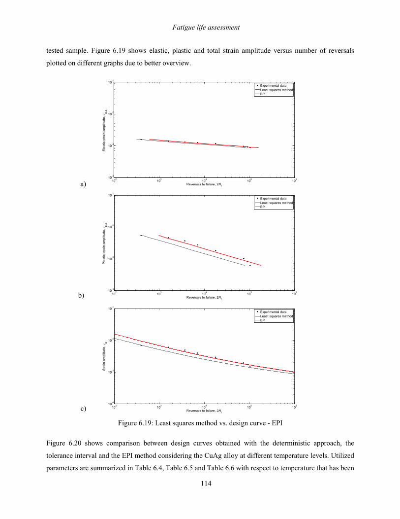
Fatigue life assessment
114
tested sample. Figure 6.19 shows elastic, plastic and total strain amplitude versus number of reversals
plotted on different graphs due to better overview.
Figure 6.19: Least squares method vs. design curve - EPI
Figure 6.20 shows comparison between design curves obtained with the deterministic approach, the
tolerance interval and the EPI method considering the CuAg alloy at different temperature levels. Utilized
parameters are summarized in Table 6.4, Table 6.5 and Table 6.6 with respect to temperature that has been
102 103 104 105 10610-4
10-3
10-2
10-1
Reversals to failure, 2Nf
Ela
stic
stra
in a
mpl
itude
, εel
,a
Experimental dataLeast squares methodEPI
102 103 104 105 10610-4
10-3
10-2
10-1
Reversals to failure, 2Nf
Pla
stic
stra
in a
mpl
itude
, εpl
,a
Experimental dataLeast squares methodEPI
102 103 104 105 10610-4
10-3
10-2
10-1
Reversals to failure, 2Nf
Stra
in a
mpl
itude
, εa
Experimental dataLeast squares methodEPI
a)
b)
c)

Fatigue life assessment
115
used during the estimation procedure. All curves consider the probability of failure β=10%. As it can be
noticed, the most conservative curve for all three temperature levels is the one calculated with the
tolerance interval, while the deterministic approach gives the less conservative curve. The tolerance
interval method is suggested to use from designing point of view to be on the safe side.
Figure 6.20: Design curves at different temperatures
102 103 104 105 10610-4
10-3
10-2
10-1
Reversals to failure, 2Nf
Stra
in a
mpl
itude
, εa
Experimental dataLeast squares methodDeterministic approachTolerance intervalEPI
102 103 104 105 10610-4
10-3
10-2
10-1
Reversals to failure, 2Nf
Stra
in a
mpl
itude
, εa
Experimental dataLeast squares methodDeterministic approachTolerance intervalEPI
102 103 104 105 10610-4
10-3
10-2
10-1
Reversals to failure, 2Nf
Stra
in a
mpl
itude
, εa
Experimental dataLeast squares methodDeterministic approachTolerance intervalEPI
T=20 oC
T=250 oC
T=300 oC
a)
b)
c)

Fatigue life assessment
116
Parameters for the deterministic approach, the tolerance interval method and for the EPI method have
been estimated considering the probability of survival equal to β=10%. Furthermore, LCF data of CuAg
alloy at three temperature levels have been used during the estimation procedure. All estimated parameters
are summarized in the following tables with respect to temperature.
Table 6.4: Estimated parameters for design curves – T=20 OC
σf'/E
(MPa) b*
εf'
c
Linear regression (β=50%) 0.00311 -0.1065 0.09485 -0.4167
Deterministic approach (β=10%) 0.00295 -0.1065 0.07201 -0.4167
Tolerance interval method (β=10%, δ=90) 0.00283 -0.1065 0.05886 -0.4167
EPI (β=10%) 0.00291 -0.1065 0.06683 -0.4167
Table 6.5: Estimated parameters for design curves – T=250 OC
σf'/E
(MPa) b*
εf'
c
Linear regression (β=50%) 0.00264 -0.1133 0.3666 -0.5551
Deterministic approach (β=10%) 0.00247 -0.1133 0.2975 -0.5551
Tolerance interval method (β=10%, δ=90) 0.00235 -0.1133 0.2506 -0.5551
EPI (β=10%) 0.00242 -0.1133 0.2769 -0.5551
Table 6.6: Estimated parameters for design curves – T=300 OC
σf'/E
(MPa) b*
εf'
c
Linear regression (β=50%) 0.00244 -0.1125 0.5747 -0.6035
Deterministic approach (β=10%) 0.00234 -0.1125 0.4626 -0.6035
Tolerance interval method (β=10%, δ=90) 0.00227 -0.1125 0.3872 -0.6035
EPI (β=10%) 0.00231 -0.1125 0.4294 -0.6035

Fatigue life assessment
117
6.10 Life assessment in terms of material models and fatigue models
Various material models, able to numerically simulate cyclic elasto-plastic material behaviour, are
described in Chapter 5. The equivalent strain range is needed to calculate in order to investigate
correlation between various material models and fatigue models. The strain is always triaxial even if in a
component the stress state is uniaxial. In case of multiaxial stress and strain states, the equivalent strain
range (Δεeq) has to be calculated:
( ) ( ) ( )2 2 2eq 1 2 2 3 3 1
23
ε ε ε ε ε ε ε∆ = ∆ − + ∆ − + ∆ − 6.41
where Δ(εi-εj) is the range of the difference between principal strains. Correction of the elastic part in
equations (6.8), (6.10) and (6.11) must be done as suggested in [Manson, 1966] before proceeding with
determination of a service life. The elastic part in equations must be shifted downward:
( ) ( ) ( )cb NNE
v ffffeq 2'2'1
32
2*
εσε+
+=
∆ 6.42
( ) 6.0f
6.012.0f
utseq 5.31
32 −− +
+=∆ NDN
Ev σε
6.43
( ) 56.0f
53.0uts155.009.0
f
832.0uts
eq 0266.017.1132 −
−−
+
+=∆ N
EDN
Ev σσε
6.44
Figure 6.21 shows the comparison between strain-life curves calculated with respect to different methods
explained so far and using parameter estimated from experimental data of CuAg alloy. The Universal
Slopes curves are obtained considering material parameters estimated from tensile test data at 20 oC and
250 oC, respectively. The Universal Slopes equation has been applied for CuAg alloy at room temperature
and at elevated temperature (T=250 oC) in this work. Although, the originally Universal Slopes equation is
suggested to use for steel at room temperature. The Modified Universal Slopes curve is obtained with
material parameters estimated from tensile test data at 250 oC. The Manson-Coffin-Basquin curve is
calculated with parameters identified from LCF data at 250 oC. As can be seen in Figure 6.21, the
Universal Slopes curve (T=20 oC - upper bound life) seems to be under conservative compared to the
Universal Slopes curve (T=250 oC). Therefore, 10% Rule (lower bound) and 20% Rule (average) are
calculated based on the Universal Slopes for T=250 oC to be on the safe side. It is worth noting how 10%
Rule seem to be over conservative, at least for this type of alloy and at this temperature. Quite
surprisingly, shape of the Modified Universal Slopes curve is very similar to the Manson-Coffin-Basquin
curve. However, the Modified Universal Slopes is situated in under conservative part. A quite good

Fatigue life assessment
118
agreement and similarity between Manson-Coffin-Basquin (250 oC) and Universal Slopes (250 oC) curves
is observed in the region beyond Δεeq=0.003.
Figure 6.21: Equivalent strain range vs. number of cycles to failure – Fatigue models
The fatigue life of the copper mould is estimated with respect to the most critical point A, described and
discussed in Chapter 5. The critical point A corresponds to the place in which occurs the highest thermal
gradient across the thickness, simultaneously causing high thermal stresses. Mechanical analyses are
performed adopting the several material models (combined model, stabilized, linear kinematic and
accelerated models), where temperature dependence of material parameters have been also taken into
consideration. The fatigue life for the most critical point A is calculated considering different material
models used in simulations as well as several fatigue curves (experimental curve 250 oC, Universal Slopes
20 oC, Universal Slopes 250 oC, Modified Universal Slopes 250 oC, 10% and 20% Rule), see Table 6.7.
102 103 104 105 10610-4
10-3
10-2
10-1
Cycles to failure, Nf
Equi
vale
nt s
train
rang
e, ∆ε
eq
CombinedStabilizedLinear kinematicAccelerated
Universal Slopes(20 oC)
Experimental data (250 oC)
10% Rule(250 oC)
20% Rule(250 oC)
Universal Slopes(250 oC)
Modified Universal Slopes(250 oC)
Table 6.7: Fatigue life estimation with respect to the critical point A and considering fatigue models
Material Models
Δεeq
Number of cycles to failure
Experimental data (250oC)
Universal Slopes (20oC)
Universal Slopes (250oC)
10% Rule (250oC)
20% Rule (250oC)
Modified Universal
Slopes (250oC)
Combined 0.00189 161141 401424 182499 959 3618 732596
Stabilized 0.00221 90147 229276 110928 717 2651 347168
Linear kin. 0.00193 148310 369460 167967 920 3471 660419
Accelerated 0.00226 82969 211020 102096 688 2543 319524

Fatigue life assessment
119
Results summarized in Table 6.7 show that similar fatigue lives are calculated with the combined and the
linear kinematic material models, regardless of the fatigue curve. This is due to fact that the combined
material model requires 60567 cycles to reach stabilized stress-strain state; its response after 20 cycles is
almost similar to the linear kinematic one. On the other hand, with the stabilized material model
plasticization phenomena area enhanced in the first cycles due to the lower yield stress, σ0*. In fact, it has
been observed in [Chaboche, 1986b] that direct use of the stabilized model could leads to heavy mistakes
especially in the case of softening materials. Therefore, the accelerated material model seems to be a good
compromise among the previously discussed approaches. Figure 6.22 shows results taken from the Table
6.7 and expressed in percentage, where 100% is a sum of fatigue lives obtained with different material
models for each fatigue model, respectively. Observing Table 6.7 and Figure 6.22 can be noticed that the
accelerated model predicts the lowest fatigue life for all 6 fatigue curves. Therefore, the accelerated
method seems suitable to use according to safe engineering design. On the other hand, the combined
material model predicts the highest life prediction.
Figure 6.22: Graphical demonstration of Table 6.7 expressed in percentage
Figure 6.23 shows the comparison between several material models (combined model, stabilized, linear
kinematic and accelerated models) and design curves (deterministic approach, tolerance interval, EPI).
Design curves are calculated considering low cycle fatigue data of CuAg alloy at T=250 oC and the
probability of failure β=10%. As in previous case, the fatigue life of the copper mould is estimated with
17% 17% 18% 21% 21%16%
31% 31% 30% 28% 28%32%
19% 19% 20% 22% 22%17%
33% 33% 32% 29% 29%36%
0%
10%
20%
30%
40%
50%
60%
70%
80%
90%
100%
Experimental data(250 °C)
Universal Slopes(20 °C)
Universal Slopes(250 °C)
10% Rule (250 °C) 20% Rule (250 °C) ModifiedUniversal Slopes
(250 °C)
Combined
Stabilized
Linear kinematic
Accelerated

Fatigue life assessment
120
respect to the most critical point A. Therefore, equivalent strain ranges in both cases are the same since the
same material models and the same critical point have been considered.
Figure 6.23: Equivalent strain range vs. number of cycles to failure - Design curves (T=250 oC)
Observing Figure 6.23 can be noticed that all design curve are situated left with respect to experimental
curve obtained with the Manson-Coffin-Basquin parameters for T=250 oC. As a consequence, all design
curves predict lowest fatigue life. However, the lowest fatigue life is predicted with the tolerance interval
curve, confirming that it is the most conservative with respect to other design curves (deterministic
approach and EPI), see Figure 6.23, Figure 6.24 and Table 6.8.
102 103 104 105 10610-4
10-3
10-2
10-1
Cycles to failure, Nf
Equi
vale
nt s
train
rang
e, ∆ε
eq
CombinedStabilizedLinear kinematicAcceleratedExperimental data
(250 oC)
Deterministic approach
EPI
Tolerance interval
Table 6.8: Fatigue life estimation with respect to the critical point A and considering design curves
Material Models
Δεeq
Number of cycles to failure
Experimental data (250oC)
Deterministic approach Tolerance interval Equivalent prediction
interval (EPI)
Combined 0.00189 161141 85130 60140 73580
Stabilized 0.00221 90147 50470 35890
43750
Linear kin. 0.00193 148310 79170 55980 68460
Accelerated 0.00226 82969 47000 33440 40750

Fatigue life assessment
121
Figure 6.24 presents results taken from the Table 6.8 and expressed in percentage, where 100% is a sum of
fatigue lives obtained with different material models for each design curve model, respectively. Based on
obtained results and in terms of design curves the tolerance interval method is suggested to use from
designing point of view to be on the safe side.
Figure 6.24: Graphical demonstration of Table 6.8 expressed in percentage
17% 18% 18% 18%
31% 30% 30% 30%
19% 19% 19% 19%
33% 33% 32% 32%
0%
10%
20%
30%
40%
50%
60%
70%
80%
90%
100%
Experimental data (250 °C) Deterministic approach Tolerance interval Equivalent predictioninterval (EPI)
Combined
Stabilized
Linear kinematic
Accelerated


Conclusions
123
Chapter 7
Conclusions
As a contribution to material modelling and parameter identification, this research work has
investigated behaviour of a component subjected to cyclic thermal loads and assessment of fatigue lives
considering several material and fatigue models, respectively. The copper mould was taken into
consideration as a case study. Therefore, the thermo-mechanical analysis of the copper mould for the
continuous steel casting was described and analysed.
Firstly, the numerical simulations and sensitivity analyses were performed, presented and described in
Chapter 3, with the aim to get the overview and the link between theoretical part and practical use of
several material models. The numerical simulations were done with respect to the three different material
models (the Armstrong and Frederick’ model, the nonlinear isotropic and the combined model). As could
be seen, the nonlinear kinematic model is able to capture monotonic hardening and Bauschinger effect;
while with the nonlinear isotropic model is possible to simulate cyclic hardening or softening phenomena.
Combination of the nonlinear kinematic and nonlinear isotropic model is appropriate for applications
subjected to cyclic loading where monotonic hardening, Bauschinger effect and cyclic hardening or
softening phenomena is needed to capture. The sensitivity analyses were shown which parameters do
really affect and how on the material response.
During the work, one of the most challenging steps was to define a suitable material model for the
thermo-mechanical analysis of a component subjected to cyclic thermal loads in order to produce
meaningful results; since amount of the resulting plastic and the elastic strain is controlled by the material

Conclusions
124
model. The combined (nonlinear kinematic and nonlinear isotropic) material model was found to be the
most suitable and reliable for applications subjected to cyclic loadings among various elasto-plastic
material models available in the literature. This was also confirmed with the numerical simulation
performed in Chapter 3. Appropriate identification procedures for the nonlinear kinematic and the
nonlinear isotropic parameters were necessary to selected before proceeding with the analysis; since
several different approaches are suggested to use in the literatures. The identification procedure for the
nonlinear kinematic and the nonlinear isotropic parameters were done separately using experimental
isothermal low-cycle fatigue data of CuAg alloy at different temperatures levels (20 °C, 250 °C, 300 °C).
During the literature review, it was observed that many authors use two and more pairs of material
parameters (Ci, γi) without explaining and justifying reasons. In this work, it was demonstrated that one
pair of material parameter (Ci, γi) provides satisfactory agreement between the experimental and the
simulated stress-strain loops. Parameters calibration should be performed step-by-step and as precise as
possible to obtain quality parameters. Using poorly estimated parameters in numerical analyses can give
misleading even wrong results what can be very dangerous, since the stress-strain response of a
component is closely related with the lifetime prediction.
Requirement of huge computational time (≈630 days) to capture the stabilized condition with the
adopted combined model was discovered once the material parameters had been calibrated and the
thermo-mechanical analysis had been performed. Since 630 days of simulation is unfeasible to perform,
some alternative material models (the stabilized, the linear kinematic and the accelerated model) were
investigated and adopted. As it is well known, the linear kinematic model is incapable to simulate cyclic
hardening or softening behaviour of a material. However, simplicity of its estimation procedure makes it
suitable to use at very early stage of the designing process to get an overview of component response;
before performing expensive and extensive experimental tests. With a further investigation, it was noticed
that direct use of stabilized model could lead to heavy mistakes, especially in the case of softening
materials. The accelerated model, which takes into consideration speed of stabilization, seemed to be a
good compromise among the previously discussed models. Based on obtained results, the accelerated

Conclusions
125
model was proposed to use when huge number of cycles are needed to simulate before reaching stabilized
condition. The accelerated model is suitable especially for industrial applications, where the choice of a
material model is usually a result of balancing and compromising between computational time, model
complexity, availability of experimental data to estimate material parameters etc.
Several strain-based fatigue models (i.e Manson-Coffin-Basquin, Universal Slopes equation, Modified
Universal Slopes equation, 10% Rule and 20% Rule) were investigated and discussed in the second part of
the thesis. The main focus was on the alternative fatigue models (Universal Slopes equation, Modified
Universal Slopes equation, 10% Rule and 20% Rule) whose parameters can be estimated using tensile test
data. These models were investigated because in most cases conducting an extensive experimental test,
especially at beginning of research, cannot be performed. The alternative fatigue models are able to
preliminary assess a fatigue life without involving prior knowledge of fatigue behaviour. However,
awareness of the facts should be present that all these fatigue models neglect some important effects as for
instance creep, influence of temperature and difference between monotonic and cyclic tests. Neglecting
some of those effects contribute of using 10% Rule and 20% Rule to be on the safe side during assessment
of a fatigue life.
Mostly in literatures, problems related with material characterization and lifetime predictions are
addressed separately. Systematic investigation is preformed considering correlation between several
material models and fatigue models as well as design curves in this work. From designing point of view,
the main intention of this research work was to point out and to clarify that sometimes in order to obtain a
survey of a component behaviour and life prediction, balance between choosing very sophisticated but
complex and simplified numerical, material and fatigue models is necessary to make. All steps should be
at the same level of approximation. First of all, developing and analysing very complex numerical models
require powerful computational memory, time, so most of the time is necessary to model and to use
simplified numerical model able to capture relevant phenomenon. Moreover, in some cases as happened in
this work, using of the most suitable and complex combined material model requires unfeasible
computational effort and time to reach the stabilized stress-strain loop.


Acknowledgments
First and foremost, I would like to express my sincere gratitude to Professor Denis Benasciutti,
Professor Francesco De Bona, Professor Mircea Gh Munteanu and PhD Luciano Moro for their
continuous support, helpful suggestions, patience and guidance throughout this research. It has been an
honor and pleasure working with You.
My sincere thanks go to the Professor Florian Grun and Aleksandar Stanojevic (Montanuniversity
Leoben, Austria) on an academic collaboration and support during the Erasmus exchange program.
I am grateful to PhD Alex Lanzutti for generously sharing his time and knowledge during
metallurgical analysis of the copper mould.
I gratefully acknowledge the members of my dissertation committee, Professors Paolo Livieri and
Saša Zelenika for their time and critical comments which enabled me to make necessary improvements of
my thesis.
Veliku zahvalnost dugujem svojim roditeljima Zlatku i Štefaniji te bratu Tomici na bezuvjetnoj podršci
tijekom cijelog školovanja, na stalnom ohrabrivanju i neizmjernoj vjeri u moj uspjeh.
I na kraju, nikada dovoljno reci HVALA mojem suprugu Velimiru na svakodnevnom strpljenju,
razumijevanju i podršci. Hvala ti što si bio uz mene u svim onim trenucima, ohrabrivao me i vjerovao u
mene.
Ovaj rad posvećujem svojoj obitelji.
Konačno ste me odškolovali!!!

129
Bibliography
[Ansoldi, 2012] Ansoldi M., Bazzaro G., Benasciutti D., De Bona F., Luvarà G., Moro L.,
Munteanu M. Gh. and Vecchiet F.: Thermo-Mechanical Analysis of a Copper
Mould for Continuous Casting of Steel, In International NT2F12 Congress,
Brasov (RO), May 2012.
[Ansoldi, 2013] Ansoldi M., Bazzaro G., Benasciutti D., De Bona F., Luvarà G., Moro L.,
Munteanu M. Gh. and Vecchiet F.: Thermo-Mechanical Analysis of a Copper
Mould for Continuous Casting of Steel. Proc. 7th Int. Conference on Low
Cycle Fatigue "LCF7", Aachen, 9-11 September 2013, pp. 527-532 (ISBN
978-3-9814516-2-7).
[ASM, 2000] ASM Handbook: Mechanical Testing and Evaluation, Vol. 8, October 2000.
[ASM, 2004] ASM International: Tensile Testing, Second edition, 2004
[ASTM] ASTM International: Standard Test Methods for Tension Testing of Metallic
Materials, E 8-04.
[Barella, 2014] Barella S., Gruttadauria A., Mapelli C., Mombelli D.: Investigation of Failure
and Damages on a Continuous Casting Copper Mould, Engineering Failure
Analysis, Vol. 36: 432-438, 2014.
[Besson, 2010] Besson J., Cailletaud G., Chaboche J. L. and Forest S.: Non-Linear
Mechanics of Materials, Springer Dordrecht Heidelberg London New York,
2010.
[Broggiato, 2008] Broggiato G. B., Campana F. and Cortese L.: The Chaboche Nonlinear
Kinematic Hardening Model: Calibration Methodology and Validation,
130
Meccanica, Vol. 43: 115-124, 2008.
[Budahazy, 2013] Budahazy L. and Dunai L.: Parameter-Refreshed Chaboche Model for Mild
Steel Cyclic Plasticity Behavior, Civil Engineering, Vol. 57, No. 2: 139-155,
2013.
[Chaboche, 1983a] Chaboche J. L. and Rousselier G.: On the Plastic and Viscoplastic
Constitutive Equations – Part I: Rules Developed With Internal Variable
Concept, Journal of Pressure Vessel Technology, Vol. 105: 153-158, 1983.
[Chaboche, 1983b] Chaboche J. L. and Rousselier G.: On the Plastic and Viscoplastic
Constitutive Equations – Part II: Application of Internal Variable Concepts to
the 316 Stainless Steel, Journal of Pressure Vessel Technology, Vol. 105:
159-164, 1983.
[Chaboche, 1986a] Chaboche J. L.: Time-Independent Constitutive Theories for Cyclic
Plasticity, International Journal of Plasticity, Vol. 2, No. 2: 149-188, 1986.
[Chaboche, 1986b] Chaboche J. L. and Cailletaud G.: On the Calculation of Structures in Cyclic
Plasticity or Viscoplasticity, Computers & Structures, Vol. 23: 23-31, 1986.
[Chaboche, 1989] Chaboche J. L.: Constitutive Equations for Cyclic Plasticity and Cyclic
Viscoplasticity, International Journal of Plasticity, Vol. 5: 247-302, 1989.
[Chaboche, 2008] Chaboche J. L: A Review of Some Plasticity and Viscoplasticity Constitutive
Theories, International Journal of Plasticity, Vol. 24: 1642-1693, 2008.
[Chen, 1988] Chen W. F. and Han D. J.: Plasticity for Structural Engineers, Springer-
Verlang, New York, 1988.
[Coffin, 1972] Coffin L. F. Jr.: Fatigue, Corporate Research and Development, General
Electric Company, Schenectady, New York, 1972.
[Desmorat, 2005] Desmorat L. R.: Engineering Damage Mechanics, Springer-Verlag, Berlin
Heidelberg, 2005.
[Dunne, 2005] Dunne F. and Petrinic N.: Introduction to Computational Plasticity,

131
University press, Oxford, 2005.
[Edward, 1997] Edward Pope J.: Rules of Thumb for Mechanical Engineers, Golf Publishing
Company, Houston, 1997.
[Elfsberg, 2003] Elfsberg J.: Oscillation Mark Formation in Continuous Casting Processes,
Royal Institute of Technology, Stockholm, Sweden, 2003.
[Franulović, 2009] Franulović M., Basan R. and Prebil I.: Genetic Algorithm in Material Model
Parameters’ Identification for Low-Cycle Fatigue, Computational Material
Science, Vol. 45: 505-510.
[Franulović, 2014] Franulović M., Basan R. and Krizan B.: Kinematic Hardening Parameters
Identification with Respect to Objective Function, International Scholarly
and Scientific Research & Innovation, Vol. 8, No. 4: 685-689, 2014.
[Gong, 2009] Gong Y., Hyde C. J., Sun W. and Hyde T. H.: Determination of Material
Properties in the Chaboche Unified Viscoplasticity Model, Proc. IMechE,
Part L: J. Materials Design and Applications, Vol. 224: 19-29, 2009.
[Halama, 2012] Halama R., Sedlak J. and Šofer M.: Phenomenological Modelling of Cyclic
Plasticity, Numerical Modelling edited by Peep Miidla, 329-351. Intech,
2012.
[Hales, 2002] Hales R., Holdsworth S. R., O’Donnell M. P., Perrin I. J. and Skelton, R. P.:
A Code of Practice for Determination of Cyclic Stress-Strain Data, Materials
at high temperature Vol. 19, No. 4: 165-185, 2002.
[Halford, 1986] Halford G. R.: Low-Cycle Thermal Fatigue, NASA Technical Memorandum
87225, Cleveland, Ohio, February, 1986.
[Halford, 1987] Halford G. R. and Saltsman J. F.: Calculation of Thermomechanical Fatigue
Life Based on Isothermal Behavior, 5th National Congress on Pressure
Vessel And Piping Technology, San Diego, California, June 28 - July 2, 1987.
[Hu, 1999] Hu W., Wang C. H. and Barter S: Analysis of Cyclic Mean Stress Relaxation
and Strain Ratchetting Behaviour of Aluminium 7050, DSTO Aeronautical

132
and Maritime Research Laboratory, Victoria, 1999.
[Imaoka, 2008] Imaoka S.: Chaboche Nonlinear Kinematic Hardening Model, Memo
Number: STI0805A, May 4, 2008.
[Khan, 1995] Khan A. S. and Huang S.: Continuum Theory of Plasticity, John Wiley &
Sons, New York, 1995.
[Koo, 2011] Koo G. H. and Kwon J. H.: Identification of Inelastic Material Parameters for
Modified 9Cr-1Mo Steel Applicable to the Plastic and Viscoplastic
Constitutive Equations, International Journal of Pressure Vessels and
Piping, Vol. 88: 26-33, 2011.
[Lee, 2005] Lee J. L., Hathaway R. B. and Barkey M. E.: Fatigue Testing and Analysis
(Theory and Practice), Elsevier Butterworth-Heinemann, 2005.
[Lee, 2009] Lee J. H, Kim K. S., Lee J. B. Yang Y. S. and Yoo M. J.: A Numerical
Simulation Model of Cyclic Hardening Behaviour of AC4C-T6 for LNG
Cargo Pump Using Finite Element Analysis, Journal of Loss Prevention in
the Process Industries, Vol. 22: 889-896, 2009.
[Lee, 2012] Lee Y. L., Barkey M. E. and Kang H. T.: Metal Fatigue Analysis Handbook,
Butterworth-Heinemann, 2012.
[Lemaitre, 1990] Lemaitre J. and Chaboche J. L.: Mechanics of Solid Materials, Cambridge
University Press, Cambridge, 1990.
[Lemaitre, 2005] Lemaitre J. and Desmorat R.: Engineering Damage Mechanics Ductile,
Creep, Fatigue and Brittle Failures, Springer-Verlag Berlin Heidelberg,
2005.
[Li, 2016] Li Mi., Barrett R. A., Scully S., Harrison N. M., Lee S. B. and O’Donoghue
P. E.: Cyclic Plasticity of welded P91 material for simple and complex power
plant connections, International Journal of Fatigue, InPress, 2016.
[Mahapatra, 1991a] Mahapatra R. B., Brimacombe J. K., Samarasekera I. V., Walker N., Paterson
E. A. and Young J. D.: Mold Behavior and Its Influence on Quality in the

133
Continuous Casting of Steel Slabs: Part I. Industrial Trials, Mold
Temperature Measurements, and Mathematical Modeling, Metallurgical
Transactions B, Vol. 22B: 861-874, December, 1991.
[Mahapatra, 1991b] Mahapatra R. B., Brimacombe J. K. and Samarasekera I. V: Mold Behavior
and Its Influence on Quality in the Continuous Casting of Steel Slabs: Part II.
Mold Heat Transfer, Mold Flux Behavior, Formation of Oscillation Marks,
Longitudinal Off-Corner Depressions, and Subsurface Cracks, Metallurgical
Transactions B, Vol. 22B: 875-888, December, 1991.
[Manson, 1965] Manson S. S.: Fatigue: A Complex Subject – Some Simple Approximations,
Experimental Mechanics, July, 1965.
[Manson, 1966] Manson S. S.: Thermal Stress and Low-Cycle Fatigue, McGraw-Hill, 1966.
[Manson, 1967] Manson S. S. and Halford G.: A Method of Estimating High Temperature
Low Cycle Fatigue Behavior of Metals, Symposium on Thermal and High
Strain Fatigue, London, 1967.
[Manson, 1968] Manson S. S.: A Simple Procedure for Estimating High-temperature Low-
Cycle Fatigue, Experimental Mechanics, Vol. 8: 349-355, 1968.
[Manson, 2006] Manson S. S. and Halford G. R.: Fatigue and Durability of Structural
Materials, ASM International, 2006.
[Manson, 2009] Manson S. S. and Halford G. R.: Fatigue and Durability of Metals at High
Temperature, ASM International, 2009.
[Martinez, 2002] Martinez W. L. and Martinez A. R.: Computational Statistic Handbook with
MATLAB, Champman & Hall/CRC, 2002.
[Marques, 2007] [Marques de Sa J. P.: Applied Statistics Using SPSS, STATISTIKA, MATLAB
and R, Springer-Verlag Berlin Heidelberg, 2007.]
[Montgomery, 2003] Montgomery D. C. and Runger G. C.: Applied Statistics and Probability for
Engineers, John Wiley & Sons, New York, 2003.

134
[Nieslony, 2008] Nieslony A., el Dsoki C., Kaufmann H. and Krug P.: New Method for
Evaluation of the Manson-Coffin-Basquin and Ramberg-Osgood Equations
with Respect to Compatibility, International Journal of Fatigue, Vol. 30:
1967-1977, 2008.
[Pajand, 2009] Rezaiee-Pajand M. and Sinaie S.: On the Calibration of the Chaboche
Hardening Model and a Modified Hardening Rule for Uniaxial Ratcheting
Prediction, International Journal of Solids and Structures, Vol. 46: 3009-
3017, 2009.
[Park, 2002a] Park J. K., Thomas B. G., Samarasekera I. V. and Yoon U.S.: Thermal and
Mechanical Behavior of Copper Molds During Thin-Slab Casting (I): Plant
Trial and Mathematical Modeling, Metallurgical and Materials Transactions,
Vol. 33B: 1-12, 2002.
[Park, 2002b] Park J. K., Thomas B. G., Samarasekera I. V. and Yoon U. S.: Thermal and
Mechanical Behavior of Copper Molds During Thin-Slab Casting (II): Mold
Crack Formation, Metallurgical and Materials Transactions, Vol. 33B: 437-
449, 2002.
[Pope, 1997] Pope E. J.: Rules of Thumb for Mechanical Engineers, Golf Publishing
Company, Houston, Texas, 1997.
[Schneider, 2003] Schneider C. R. A. and Maddox S. J.: Best Practice on Statistical Analysis of
Fatigue Data, International Institute of welding, Camridge UK, 2003.
[Schijve, 2001] Schijve J.: Fatigue of Structures and Materials, Kluwer Academic
Publishers, Dordrecht, 2001.
[Silvestre, 2015] Silvestre E., Mendiguren J., Galdos L. and Saenza de Argandona E.:
Comparison of the Hardening Behaviour of Different Steel Families: from
Mild and Stainless Steel to Advanced High Strength Steels, International
Journal of Mechanical Sciences, July, 2015.
[Stephens, 2001] Stephens R. I., Fatemi A., Stephens R. R. and Fuchs H. O.: Metal Fatigue in
Engineering, John Wiley & Sons, New York, 2001.

135
[Suresh, 1998] Suresh S.: Fatigue of Materials, Cambridge University Press, 1998.
[Thomas, 1997] Thomas B. G., Li G., Moitra A. and Habing D.: Analysis of Thermal and
Mechanical Behaviour of Copper Molds During Continuous Casting of Steel
Slabs, 80th Steelmaking Conference, Chicago (IL), April 1997.
[Thomas, 2002] Thomas B. G.: Modeling of the Continuous Casting of Steel – Past, Present,
and Future, Metallurgical and Material Transactions, Vol. 33B: 795-812,
2002.
[Tong, 2003] Tong J. and Vermeulen B.: The Description of Cyclic Plasticity and
Viscoplasticity of Waspaloy Using Unified Constitutive Equations,
International Journal of Fatigue, Vol. 25: 413-420, 2003.
[Tong, 2004] Tong J., Zhan Z.-L. and Vermeulen B.: Modelling of Cyclic Plasticity and
Viscoplasticity of a Nickel-Based Alloy Using Chaboche Constitutive
Equations, International Journal of Fatigue, Vol. 26: 829-837, 2004.
[Williams, 2003] Williams C. R., Lee Y.-L. and Rilly J. T.: A practical method for statistical
analysis of strain-life fatigue data, International Journal of Fatigue, Vol. 25.:
427-436, 2003.
[Wirsching, 1980] Wirsching P. H., ASCE A. M. and Hsieh S.: Linear Model in Probabilistic
Fatigue Design, Journal of the Engineering Mechanics Division, Vol, 106:
1266-1278, 1980.
[Wirsching, 1983] Wirsching P. H.: Statistical Summaries of Fatigue Data for Design Purpose,
NASA Contractor Report 3697, 1983.
[You, 2008] You J. H. and Miskiewicz M.: Material Parameters of Copper and CuCrZr
Alloy for Cyclic Plasticity at Elevated Temperatures, Journal of Nuclear
Materials, Vol. 373: 269-274, 2008.
[Zaletelj, 2011] Zaletelj H., Fajdiga G. and Nagode M.; Numerical Methods for TMF Cycle
Modeling, Journal of Mechanical Engineering, Vol. 54: 458-494, 2011.
[Zhao, 2001] Zhao L. G., Tong B., Vermeulen B. and Byrne J.: On the Uniaxial

136
Mechanical Behavior of an Advanced Nickel Based Superalloy at High
Temperature, Mechanics of Materials, Vol. 33: 593-600, 2001.


