Political decentralization and corruption: Evidence from around the world

How does political decentralization affect the frequency and costliness of bribe-extraction by corrupt officials? Previous empirical studies, using subjective indexes of perceived corruption and mostly fiscal indicators of decentralization, have suggested conflicting conclusions. In search of more precise findings, we combine and explore two new data sources—an original cross-national data set on particular types of decentralization and the results of a firm level survey conducted in 80 countries about firms’ concrete experiences with bribery. In countries with a larger number of government or administrative tiers and (given local revenues) a larger number of local public employees, reported bribery was more frequent. When local—or central—governments received a larger share of GDP in revenue, bribery was less frequent. Overall, the results suggest the danger of uncoordinated rent-seeking as government structures become more complex.

C. Simon Fan, Lingnan University, Hong Kong Chen Lin, Lingnan University, Hong Kong

and Daniel Treisman, UCLA

September 2008

Corresponding author: Professor Daniel Treisman, Department of Political Science, University of California, Los Angeles, 4289 Bunche Hall, Los Angeles, CA 90095-1472. Tel: 310.968.3274; Fax: 310.825.0778; email: treisman@polisci.ucla.edu. We thank Robin Boadway (the editor) and two anonymous referees for many constructive comments and suggestions that have helped improve the quality of the paper a lot.

1

1 Introduction

How does political decentralization affect the frequency and the costliness of corrupt bribe-extraction by

officials? Theories suggest conflicting conclusions. On one hand, by bringing officials “closer to the

people” or encouraging competition among governments for mobile resources, decentralization might

increase government accountability and discipline. On the other, decentralization could impede

coordination and exacerbate incentives for officials at different levels to “overgraze” the common bribe

base. More generally, one might expect a variety of effects associated with different types of

decentralization to operate simultaneously, pulling in many directions, with different strength in different

contexts.

A number of scholars have sought to answer this question empirically by looking for relationships

between measures of political or fiscal decentralization and crossnational indexes of perceived corruption

derived from surveys of risk analysts, businessmen and citizens. In particular, scholars have examined

perceived corruption ratings produced by Transparency International (TI), the World Bank (WB), and the

business consultancy Political Risk Services, which publishes the International Country Risk Guide

(ICRG). The findings of these studies have been mixed and sometimes mutually contradictory.

Focusing on fiscal decentralization, Huther and Shah (1998), De Mello and Barenstein (2001),

Fisman and Gatti (2002), and Arikan (2004) all report that a larger subnational share of public

expenditures (as measured in the IMF’s Government Finance Statistics) was associated with lower

perceived corruption using the TI, ICRG, or WB indexes. Enikolopov and Zhuravskaya (2007) do not

report an unconditional effect, but find that a larger subnational revenue share is associated with lower

perceived corruption (using WB, but not TI, data) in developing countries with older political parties (and

vice versa); a larger subnational revenue share in developing countries where there are few parties in

government is associated with lower corruption (on both WB and TI measures) (and vice versa). Looking

at political rather than fiscal indicators, Goldsmith (1999), Treisman (2000), and Kunicová and Rose

Ackerman (2005) all found that federal structure was associated with higher perceived corruption.

2

However, in a more recent review of the empirical literature, Treisman (2007) suggested that neither the

(negative) expenditure decentralization effect nor the (positive) federalism effect was robust. The fiscal

decentralization effect was weakened by controlling for national religious traditions, and the federal effect

disappeared as the number of countries in the sample increased. Treisman (2002) and Arikan (2004)

explored whether smaller local units were associated with less corruption because of more intense

interjurisdictional competition, but obtained inconclusive results. Finally, examining the effect of the

vertical structure of states, Treisman (2002) found that a larger number of administrative or governmental

tiers correlated with higher perceived corruption, but whether subnational governments were appointed or

elected did not have a clear effect.

In this paper, we advance and improve upon this literature in three ways. First, our analysis exploits

an original cross-national data set on different varieties of decentralization, compiled from more than 480

sources. This allows us to design indicators of particular types of decentralization to match the underlying

logic of specific arguments. We look for relationships between reported experience with corruption and:

(i) the number of tiers of government or administration in the country (see Section 3.1), (ii) the average

land area of lowest tier units (see Section 3.2), (iii) several proxies for the extent of subnational political

decisionmaking (see Section 3.2 and others), (iv) an indicator for whether lower tier units have elected

executives (see Section 3.3), (v) a measure of subnational tax revenues as a share of GDP (see Section

3.4), and (vi) an estimate of the share of subnational government personnel in total civilian government

personnel (see Section 3.5).

Second, most previous studies have used perceived corruption indexes that rely on the aggregated

perceptions of businessmen or country experts, many of whom may have formed impressions—perhaps

subconsciously—based on common press depictions of countries or conventional notions about what

institutions or cultures are conducive to corruption. More recently, a second type of data has become

available: survey responses of businessmen and citizens in particular countries about their own (or close

associates’) concrete experiences with corrupt officials. In a recent study, Treisman (2007) showed that,

for developing countries, the perceived corruption indexes were relatively weakly correlated with

3

experience-based indicators. Among countries rated as highly corrupt on the subjective indexes of TI,

WB, and the ICRG, there is great variation in the level of reported experience with corruption. For

instance, on the World Bank perceived corruption index, Argentina and Macedonia were both rated about

equally corrupt in 2000: they were ranked 103 and 114 respectively out of 185 countries. But respondents

from these two countries gave dramatically different answers when surveyed by the United Nations

Interregional Crime and Justice Research Institute (UNICRI) in the late 1990s about their own personal

experience with bribery. When asked whether during the previous year “any government official, for

instance a customs officer, police officer or inspector” had asked or expected them to pay a bribe for his

services, respondents in Argentina were three and a half times as likely as the Macedonian respondents to

say yes. While Argentina had the second highest frequency of reported demands for bribes (second only

to Indonesia), Macedonia was only 24th in the list of 49 countries, about even with South Africa and the

Czech Republic. Perhaps of greater concern, a number of factors commonly believed to affect corruption

(democracy, press freedom, oil rents, even the percentage of women in government) do an excellent job

explaining the cross-national varietion in the subjective corruption indexes (R-squareds approaching .90).

But the same factors are mostly uncorrelated with the frequency or scale of self-reported experiences with

corruption once one controls for income. One cannot help wondering if the businessmen and experts

whose perceptions are being tapped might be inferring corruption levels from its hypothesized causes.

In this study, we explore the results of an experience-based survey of business managers conducted

in 80 countries. The World Business Environment Survey interviewed managers from more than 9,000

firms in 1999-2000. We focus on two questions. Respondents were asked: “Is it common for firms in your

line of business to have to pay some irregular ‘additional payments’ to get things done?” and “On

average, what percent of total annual sales do firms like yours typically pay in unofficial payments/gifts

to public officials?” The first question provides an indicator of the frequency of bribery, while the second

aims to estimate its scale. The relationship between the proportion of respondents that said irregular

payments were expected “always”, “mostly”, or “frequently”, and the World Bank’s subjective index of

perceived corruption for the year 2000 are graphed in Figure 1. It is interesting to note that while

4

businessmen in France and Brazil gave very similar responses to this question (about 27 percent saying

bribes were expected “always”, “mostly”, or “frequently”), France is rated as among the least corrupt

countries on the World Bank’s index, while Brazil is perceived to have much higher corruption. Of

course, no approach is completely without problems; it is possible that questions that focus more closely

on managers’ direct experience with corruption might not be answered with complete frankness for fear

of some kind of self-incrimination. However, we believe this danger is less serious than the danger that

bias will creep into the assessments of “experts” and foreign businessmen because of inconsistencies in

media coverage. (As a robustness check, we compare our results to those obtained using the traditional

perceived corruption data.)

[Figure 1 here]

Third, besides permitting us to focus on experience-based rather than subjective indicators of

corruption, the WBES makes it possible to control better for individual characteristics of survey respondents

(which vary systematically across countries). Specifically, we can control for the size, ownership structure,

investment level, and level of exports of firms in analyzing their managers’ responses on corruption.

In the next section, we briefly introduce the decentralization data used in the paper. We review common

arguments about the consequences of decentralization for governance in section 3, and in section 4 discuss the

corruption data and controls. We then look for evidence of the hypothesized effects in the WBES. In Section

5 we present empirical results and discuss robustness tests. Section 6 discusses the findings and concludes.

2 A new data set on governance in multi-level states

Previous work has often used measures of fiscal decentralization or simple dummies for federal structure to

proxy for various other types or dimensions of political and administrative decentralization. The data set

introduced here permits a more fine-grained analysis. It contains measures of various characteristics of

multi-level states as of the mid-1990s, based on information from more than 480 sources.1

1 These data and the full list of sources will be made available on the corresponding author’s web site.

5

A first dimension is simply the number of tiers of government or administration. Our data set contains

information on this for 156 countries. We coded a level of administration as a “tier” if there existed a state

executive body at that level which met three conditions: (1) it was funded from the public budget, (2) it had

authority to administer a range of public services, and (3) it had a territorial jurisdiction. This definition

includes both bodies with decisionmaking autonomy and those that are essentially administrative agents of

higher level governments. On this measure, Singapore as of the mid-1990s had just one tier, while Uganda

had six.

Multi-level states differ also in the number and size of their lowest-tier units. This is relevant, for

instance, to arguments about interjurisdictional mobility. The data set contains estimates of the number of

bottom level units (BOTTOM UNITS), and the “average” area of these (BOTTOM SIZE), calculated by simply

dividing the country’s area by the number of units.2 While Guyana in the mid-1990s had just six incorporated

towns, India had some 235,000 lower tier village governments. The average area of the lowest tier units

ranged from 2.2 square kilometers in Bangladesh to 83 square kilometers in Botswana.

Perhaps most important, multi-level governments differ in how authority is divided among the various

tiers. Measuring the degree of decisionmaking autonomy of local governments in a systematic way is

notoriously difficult. Our data set contains a simple dummy (AUTONOMY), which records for 133 countries

whether the constitution assigned at least one policy area exclusively to subnational governments or gave

subnational governments exclusive authority to legislate on matters not constitutionally assigned to any level.

This variable is less than ideal. For one thing, informal behavior often diverges from what is written in the

constitution. In some countries—Azerbaijan and Uzbekistan, for instance—it seems unlikely the

constitutional provisions are scrupulously observed.3 Yet determining the degree of actual decisionmaking

decentralization in any country is inescapably subjective. Experts often disagree with regard to a single

country, let alone agreeing on crossnational comparisons. At the same time, the number and relative

2 A better variable would be the average area of all actual units, but data were not available. Since the number of bottom-tier units changes over time as units split or combine, the variable is only a rough indicator. 3 Both inherited Soviet-era internal “autonomous republics”, whose rights are constitutionally protected.

6

importance of policy areas constitutionally assigned to subnational governments differs, and there is no

obvious way to add these up. AUTONOMY also focuses mostly on intermediate levels—states, provinces, or

regions—whereas the governments most relevant to questions of interregional competition will often be at the

local level. We supplement the use of AUTONOMY in our analysis with several other indicators of

decisionmaking decentralization available from other data sets and sources.4

To capture differences in the extent of local electoral accountability, we constructed two variables. The

first (BOTTOM TIER ELECTION) focuses on the mode of selection of the chief executive of the bottom tier

government, while the second (SECOND LOWEST TIER ELECTION) focuses on the executive at the next

highest tier. Each of these takes the value 1 if the executives at the relevant tier were (as of the mid-1990s)

directly elected or chosen by a directly elected local assembly, and 0 if the executives were appointed by

higher level officials. They take the value 0.5 if some chief executives were appointed while others were

elected.

Details of the variables and the correlations between them and some other common decentralization

indicators are shown in Tables 1 and 2. While we focus on the impact of political decentralization on

corruption in this study, the political decentralization measures introduced here could be used to examine the

effects of decentralization on various other aspects of government performance such as service quality,

provision of public goods, and tax collection.

[Tables 1 and 2 here]

3 Decentralization and corruption: theory

Political or fiscal decentralization might affect the quality of government in various ways. We discuss

4 Our definition of AUTONOMY is close to various classic definitions of federalism. Riker (1964) defines states as “federal” if: (1) they have (at least) two levels of government, and (2) each level has “at least one area of action in which it is autonomous.” The latter requirement must be formally guaranteed, for instance in a constitution (Riker 1964, p.11). This is close to Robert Dahl’s definition of federalism as “a system in which some matters are exclusively within the competence of certain local units—cantons, states, provinces—and are constitutionally beyond the scope of the authority of the national government; and where certain other matters are constitutionally outside the scope of the authority of the smaller units” (Dahl 1986, quoted in Stepan 2001, p.318; italics in original). In our operationalization, AUTONOMY is a broader category because we assign a “1” also to countries that devolve decisionmaking rights to certain selected regions but not to others.

7

here a number of arguments made in previous work, specifying to which type of decentralization each

applies. We do not expect most to be fully general, and some could operate simultaneously or offset each

other in complicated ways.

3.1 Vertical competition

Governments can use the power to regulate to extract bribes from firms or citizens. If the bribe rate is set too

high, this will discourage firms or citizens from producing wealth, reducing the amount of revenue actually

extracted. Thus, a unitary predatory government will moderate its demands. However, if multiple officials

regulate the same actors and fail to coordinate, they may set the total bribe rate higher than would be optimal

for a unitary, bribe-maximizing government (Shleifer and Vishny 1993). Indeed, the aggregate bribe burden is

likely to increase with the number of independent regulators. If officials at each tier in a multi-level state can

regulate, the burden of bribery should increase with the number of tiers. The logic is that of “double

marginalization” under vertical integration (Spengler 1950) or “overgrazing” in taxation (Keen and

Kotsogiannis 2002, Berkowitz and Li 2000).5

Although appealing, this argument might fail for various reasons. The number of independent

regulators might not increase with the number of tiers. In fact, administrative complexity at the center and

decentralization might be substitutes—to govern directly, a central government may need to create more

agencies in the capital to take the place of local field agents. Moreover, career concerns might motivate local

officials in a decentralized state to behave honestly. The hope of rising to higher office may cause local

officials to cultivate a reputation for integrity (Myerson 2006). Finally, if elected governments at different

levels provide comparable public goods, some scholars suggest they may be disciplined by yardstick

competition. Voters can use the performance of each as a benchmark to judge the efficiency of the other

(Salmon 1987, Breton 1996, p.189). If one government over-regulates in order to extract bribes, its

5 In a notable recent contribution, Olken and Barron (2007) find evidence consistent with double-marginalization using Indonesian data.

8

performance will look bad in comparison to its more liberal counterparts at other levels. To test this argument,

we use the variable TIERS, measuring the number of levels of government or administration.

3.2 Interregional competition If capital or labor is mobile and local governments choose policies, they may tailor these to attract the mobile

factor (Hayek 1939, Tiebout 1956). Officials who steal or waste resources will lose residents and businesses

to other regions, reducing their tax base. If they over-regulate in order to extract bribes, firms will flee to

lower-regulation settings. In this way, interjurisdictional competition may discipline local governments,

reducing corruption and causing them to supply public goods efficiently (Brennan and Buchanan 1980;

Montinola et al. 1995). The impact of such competition should be greater, the lower the cost of moving

between units; moving costs should increase with the size of the units.

However, the fear of losing mobile capital may fail to discipline local governments for a number of

reasons (e.g., Cai and Treisman 2005). Or governments may compete to attract capital by promising corrupt

benefits to local businesses at the expense of the central government (Cai and Treisman 2004). Even if

interjurisdictional competition motivates local politicians to reduce corruption, it does not increase their

capacity to do so. If most bribes are taken by local bureaucrats and anti-corruption measures must be

implemented by the same bureaucrats, it may matter little how motivated the politicians are to clean up

government. And if anti-corruption measures are costly, the inability to tax mobile capital may make it harder

for local governments to fund such efforts.

The relevant type of decentralization here is devolution of decisionmaking about regulation or taxation

to subnational levels; among countries with a similar level of such devolution, one might expect a positive

correlation between average size of the subnational units and corruption. To measure devolution of

decisionmaking, we start with the variable AUTONOMY. But we supplement it with various alternatives.

First, we created a dummy for whether the country was classified as “federal” by a leading expert on

federalism as of the mid-1990s (FEDERAL) (Elazar 1995). Second, in an attempt at a more fine-grained

9

analysis, we tried using measures of the extent of decisionmaking decentralization in specific public service

areas, constructed by Henderson (2000). Henderson coded whether, in 49 countries in 1960-95, authority for

primary education, local highway construction, and local policing belonged to the central, regional, or local

governments, or some combination of the three.6 (Of these 49 countries, 35 were included in the WBES.)

Both local road construction and local policing could impinge on the operations of almost any business, but it

is harder to see how the regulation of primary schooling could lend itself to widespread extraction of bribes

from businesses, so we focused on the former two indicators. We constructed two variables (ROADS LOCAL

and POLICE LOCAL) which took the value 1 if, as of 1995, the local governments participated in

decisionmaking on the issue in question, and 0 otherwise.7 The arguments in Section 3.2 suggest that when

ROADS LOCAL and/or POLICE LOCAL equal one, greater factor mobility might be associated with lower

corruption. To capture the average size of subnational units, which should be positively related to moving

costs, we used our variable BOTTOM SIZE.

3.3 Electoral accountability For several reasons, holding elections at the local level rather than just the center might increase the

accountability of government (see e.g. Seabright 1996). First, voters might have better information about local

than about central government performance. Second, whereas national elections focus on government

performance nationwide, local elections can focus more specifically on performance in each region. Third,

dividing up responsibilities among several levels of elected government might make it easier for voters to

attribute credit or blame among them (under decentralization, one can vote for an honest central government

6 The details of the data set constructed by Henderson (2000) can be obtained through direct communications with Henderson. 7 In only one case—local highway construction in Uganda—did the local governments enjoy exclusive authority. We also constructed an indicator (SHARED RESPONSIBILITY) for the number of government levels participating in decisionmaking in these two policy areas (the more governments involved, the greater the potential for predatory extraction and “overgrazing”). Values ranged from 2 if for both local highways and policing only one level could make policy (as in Syria or Egypt), to 6 if, for both areas, all three levels of government could participate (as in the US). From the arguments in Section 3.1, one might expect SHARED RESPONSIBILITY to correlate positively with corruption. In fact, it was never significant, so we do not show results including it.

10

and against a corrupt local government rather than having to vote for or against the team as a whole).8 Fourth,

the smaller a unit’s electorate, the easier it should be for voters to coordinate on a voting strategy to discipline

the incumbent.

Questions can be raised about each of these arguments. First, local corruption can be concealed at least

as well as central corruption, and watchdog groups and investigative journalists tend to devote more resources

to monitoring national government since the stakes are generally higher. Second, voters evaluate incumbents

on multiple dimensions and it is not clear whether corruption will be more salient in local or in national

elections. Even if voters voted on just the corruption question, competition in a national election should often

motivate central candidates to fight corruption in each district (if they do not, their adversary will, winning

votes in the affected unit). Third, dividing responsibilities among levels may muddle rather than clarify the

attribution of responsibility (compare a system in which two levels share responsibility for all policy areas to

one in which a central government is alone responsible for all). Finally, coordinating is only significantly

easier in groups that are very small (and smaller than the electorates of most existing local districts). Even in

tiny villages, there are many dimensions on which voters could judge local officials, rendering coordination to

discipline them on corruption problematic.9 To capture differences in the extent of local electoral

accountability, we used the variables BOTTOM TIER ELECTION and SECOND LOWEST TIER ELECTION.

3.4 Fiscal incentives

The greater is corruption, the lower will be the motivation of firms to produce. Given this, some argue

that corruption will fall if local officials are given a large personal stake in local economic activity. Under

tax-sharing systems, the larger the share local governments retain of marginal tax revenues, the lower

8 Besley and Coate (2003) make a similar argument about why direct election of regulators—rather than their appointment by elected officials—might lead to greater responsiveness to voters by reducing the number of issues on which each vote is cast. 9 Electoral decentralization also eliminates accountability of local officials to voters outside their unit, which might itself increase some kinds of corruption. A locally elected sheriff could increase his town’s revenues, taking a cut for himself, by inaccurately citing out-of-town motorists for speeding.

11

should be their incentive to extract bribes (Montinola, Qian, and Weingast 1995, Zhuravskaya 2000, Jin et

al. 2005). Since the argument relates to the marginal rate at which local governments benefit from

increased local business activity, the relevant variable is the local governments’ revenue as a share of

local income at the margin. As usual, there are caveats. Increasing local governments’ share means

decreasing the shares of other levels. If local governments become more motivated to support economic

performance, governments at other levels should become less motivated. Since, for better or worse,

governments at all levels influence economic performance, the resulting net effect is indeterminate

(Treisman 2006). Moreover, local officials may derive greater utility from bribe revenue, which they can

spend at will, than from increased revenue officially received by the local budget, which may be costly to

embezzle. If officials are already constrained by the risk of detection from embezzling more, then

increasing the local tax share may not make them want to reduce their bribe taking in order to expand the

local budget.

To test this argument, we use subnational government revenues as a percentage of GDP. The data

are mostly from the IMF’s Government Finance Statistics Yearbooks (as collected in the World Bank’s

database of fiscal decentralization indicators), supplemented by additional sources on specific countries.

We took the average value for all available years between 1994 and 2000. There are some missing

observations in this variable so the sample size falls from 67 countries (6,676 observations) to 54

countries (5,598 observations) when we include it. Some previous studies used a variable measuring the

share of local revenues or expenditures in total public revenues or expenditures to look for the effects of

fiscal decentralization. However, since the argument here concerns the share of local income that local

governments retain through taxation, we prefer an indicator that measures this more closely—the share of

local revenues in GDP.

A better variable would have been the marginal revenue rate for local governments from locally

generated income; however, cross-national data on marginal rates were not available, so we had to use the

average rate instead. We control in these regressions for total government revenues as a share of GDP,

since larger government might be associated with both greater corruption and higher local taxation.

12

3.5 Local collusion

Some economists suggest local officials are simply more susceptible to corruption than their central

counterparts, perhaps because they have more opportunities for face-to-face interactions with businessmen

(e.g., Prud’homme 1995, Tanzi 1995, Bardhan and Mookherjee 2000) Local press and citizen groups may be

weaker—and more subject to intimidation or cooptation—than at the center. Interest groups may be more

cohesive at the local level, leading to greater state capture. By this logic, government should be more corrupt,

the greater the share of government personnel located at subnational levels.

However, one could also argue the opposite. Even if the intimacy of interaction and the cohesiveness of

interest groups are greater at the local level, the potential kickbacks and payoffs in national politics are likely

to be higher. As noted in Section 3.3, voters are often assumed to be better informed about their local

governments than about politics in the nation’s capital. In any case, the real question is not whether local

governments are likely to be more corrupt than central governments but whether elected local governments

with decisionmaking power are likely to be more or less corrupt than centrally appointed local agents with

more restricted authority. Whether there is a general answer to this question is unclear. To test this argument,

we constructed a measure of government personnel decentralization—the subnational share in total civilian

government employees as of the mid-1990s, as estimated by Schiavo-Campo et al. (1997). We control for

total government employment as a share of the labor force, since, as noted, the size of government as a whole

might itself be related to corruption.

4 Corruption data and controls

4.1 The survey

The WBES was conducted in 1999 and 2000 by a team from the World Bank. Managers from over 9,000

firms in more than 80 countries were surveyed with a standard questionnaire.10 The main purpose was to

identify the driving factors behind and obstacles to enterprises’ performance and growth around the world.

10 For more information on the survey, see http://www.ifc.org/ifcext/economics.nsf/Content/ic-wbes.

13

The questionnaire touched on many aspects of firms’ operations, including corruption, regulation, and the

institutional environment. The firms surveyed varied in size (including a large number of small and

medium-size enterprises), ownership (both public and private), industrial sector, and organizational structure.

Because of missing firm-level and decentralization variables, the number of firms we could include in our

analysis starts at about 6,700 (from 67 countries), and falls lower as additional variables are added. Previous

work has used the WBES data to study such outcomes as firm growth, investment flows, the effects of

institutions, property rights, and corruption (Hellman, Kaufman, and Schankerman, 2000; Djankov, La Porta,

Lopez-De-Silanes, and Shleifer, 2003; Beck, Demirguc-Kunt and Maksimovic, 2005; Acemoglu and Johnson,

2005; Beck, Demirguc-Kunt and Levine 2006; Ayyagari, Demirguc-Kunt and Maksimovic, 2007, Barth, Lin,

Lin and Song, 2008). According to Reinikka and Svensson (2006, p.367), the WBES shows that “with

appropriate survey methods and interview techniques, it is possible to collect quantitative data on corruption

at the micro-level.”

4.2 Measures of corruption

We constructed two measures of corruption using WBES data. The first, which we call BRIBE

FREQUENCY, is based on a question in which respondents were asked: “Is it common for firms in your

line of business to have to pay some irregular ‘additional payments’ to get things done.” The interviewers

assured respondents that their responses would be kept completely confidential, and that their names and

the names of their firms would never be identified in any publication or survey document. In addition, to

encourage honest responses, the question asked only about unofficial payments “in your line of business”

rather than those “paid by your firm” (Johnson, McMillan and Woodruff 2002). Managers could choose

between six responses: 1 (never), 2 (seldom), 3 (sometimes), 4 (frequently), 5 (usually), and 6 (always).

Thus, the variable BRIBE FREQUENCY takes these six values; a larger value represents more frequent

bribery payments.11 Overall, about 69 percent of respondents (6,300 out of 9,130) reported that firms like

theirs paid bribes to public officials to get things done. About 15 percent of the firms reported that this

11 The original survey offered the six choices in reverse order: (1) always, (2) mostly, (3) frequently, (4) sometimes, (5) seldom, (6) never. We recoded the variable to make the empirical results more intuitive.

14

occurred “4 ( frequently),” 12 percent reported “5 (usually),” and 9 percent reported “6 (always)”. In

countries such as Bangladesh, Nigeria, Tanzania, Thailand, Uganda, and Zimbabwe, more than 90 percent

of the firms sampled reported that such unofficial payments occurred at least occasionally. The lowest

rate of reported bribery was in Singapore, where 90 percent said firms like theirs never had to make

unofficial payments.

Our second measure, which we call BRIBE AMOUNT, was constructed from a question that asked:

“On average, what percent of total annual sales do firms like yours typically pay in unofficial

payments/gifts to public officials?” The survey offered seven choices: (1) 0 percent, (2) 0-1 percent, (3)

1-1.99 percent, (4) 2-9.99 percent, (5) 10-12 percent, (6) 13-25 percent, and (7) over 25 percent. Out of

the original sample of 80 countries, respondents in 60 countries answered this question. Overall, more

than 62 percent of those who responded reported that firms like theirs typically made positive unofficial

payments to public officials. More than 38 percent reported that such payments were greater than 1

percent of total sales; about 11 percent said payments exceeded 10 percent of total sales. The average size

of such payments varied across both countries and the firms within them.

The two measures of corruption are complementary, capturing different dimensions that may not

always coincide (bribes could be frequent but tiny, or rare but large). In some respects, the amount of

bribes paid is the more interesting variable. However, it was also apparently perceived by respondents as

more sensitive: in one quarter of the countries, respondents did not answer this question. By contrast, the

response rate for the first question was high: the only country in which none answered the question was

China, and the response rate ranged from 63 percent in Senegal to 100 percent in the Philippines and

Thailand, with an average of 92 percent.12 Consequently, our regressions of BRIBE FREQUENCY can

include a larger range of countries than those for BRIBE AMOUNT. As will become clear, our results

using the two variables are very similar and complementary. 12 In order to further explore the potential issue of non-randomly missing responses, we created a truncated sample from which all the firms that were missing observations on any of the following key variables were excluded: corruption frequency, firm size, government ownership, foreign ownership and exporting status. We then compared the truncated sample to the full sample for the same firm characteristics. (Since many were missing data on just one of these, the full sample could differ substantially from the truncated sample.) In all cases, the differences between the truncated sample and full sample were not statistically significant. We also tried dropping some countries with relatively high missing response rates (e.g. Senegal) from the sample and found the empirical results highly robust.

15

The WBES also asked respondents about the particular contexts in which bribes were demanded.

Specifically, it asked whether “firms like yours typically need to make extra, unofficial payments to

public officials for any of the following purposes…” and listed six possibilities: “to get connected to

public services (electricity, telephone), to get licenses and permits, to deal with taxes and tax collection, to

gain government contracts, when dealing with customs/imports, and when dealing with courts”. For each

of these, respondents could choose from six answers: 1 (never), 2 (seldom), 3 (sometimes), 4 (frequently),

5 (usually), and 6 (always). We constructed variables for the first five (Public Services, Business License,

Tax Collection, Government Contract, and Customs, respectively), and repeated our analysis to see if

decentralization had different effects on corruption in these different settings. We did not expect to find

similar results for corruption of the courts, since the arguments that apply to executive officials fit less

well in this case. As a check to increase confidence that some unobserved third factor is not driving the

results, we also ran regressions for the courts variable, and show that the results for executive officials do

not extend to the courts.

4.3 Firm-level control variables

In our regressions, we include dummy variables for firms’ ownership. The variable State Ownership

equals 1 if any government agency or state body has a financial stake in ownership of the firm, 0

otherwise. Foreign Ownership equals 1 if a foreign company or individual has a financial stake in

ownership of the firm, 0 otherwise. The excluded category consists of firms completely owned by

domestic private businesses or individuals. We expect that private firms are more vulnerable to bribe

demands because they tend to have fewer government connections, less political influence, and weaker

bargaining power (Svensson 2003). We also control for whether the given enterprise is an exporter

(Exporter equals 1 if the firm exports, 0 otherwise) and for the enterprise’s size (Firm Size equals the

natural logarithm of firm sales). Finally, we include industry classification dummies (for manufacturing,

services, agriculture, construction, other); to save space, we do not report the coefficients on these.

16

4.4 Country-level control variables

Previous studies have found certain aspects of countries’ economic structure, institutions, and culture to

be significantly related to indicators of perceived corruption. La Porta et al. (1999), Ades and Di Tella

(1999), Svensson (2005), and many others found robust evidence that higher GDP per capita was

associated with lower perceived corruption. Treisman (2000) reported that Protestant religion, a history of

British rule, and a long exposure to democracy were significantly linked to lower perceived corruption.

Ades and Di Tella (1999) found that corruption was perceived to be greater in countries with large

endowments of valuable natural resources (e.g. fuel and minerals) and in those that were less open to

trade. Following previous practice, we control for the logarithm of countries’ GDP per capita (GDP per

Capita), imports of goods and services as a share of GDP (Imports), democracy in all years between 1950

and 2000 (Democratic), status as a former British colony (British Colony), share of minerals and fuels in

manufacturing exports (Fuel), and the proportion of Protestants in the population (Protestant). To check

for robustness, we try also including the number of years the country had been open to trade, a variable

for presidential system, and an index of press freedom constructed by Freedom House. The empirical

results were very robust to including these variables.13 Table 3 provides brief descriptions of the variables

and data sources. Table 4 presents summary statistics.

[Tables 3 and 4 here]

5 Results

5.1 Basic models

We estimate two sets of regressions, one using the dependent variable BRIBE FREQUENCY, the other

using BRIBE AMOUNT. In each case, we assume the enterprise’s latent response can be described as

follows:

13 For brevity, we do not report these results here; both the number of years open to trade and the press freedom index were significantly associated with lower corruption.

17

, 1 , 2 ,

3 , 4 , 5 ,

'

i j j i j i j

i j i j i j

DEPVAR Decentralization Measures State Foreign

Exporter Firm Size Industry Dummies

, ' j i jCountry Controls

(1)

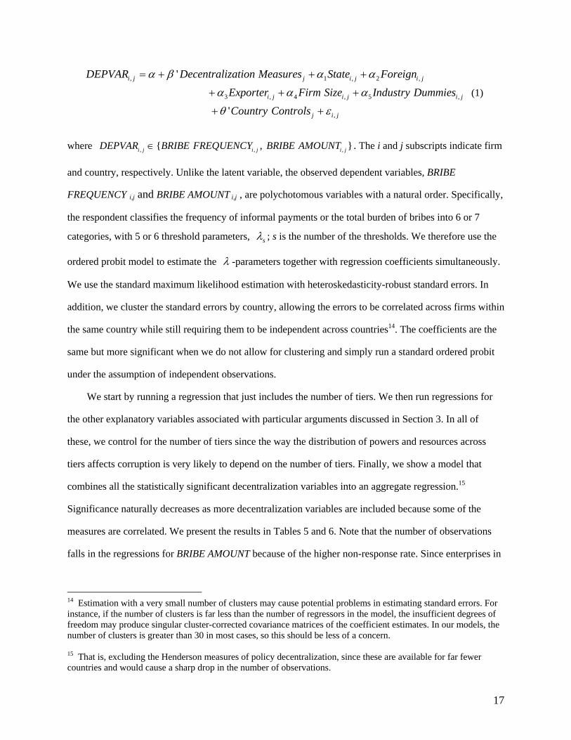
where , , ,{ , }i j i j i jDEPVAR BRIBE FREQUENCY BRIBE AMOUNT . The i and j subscripts indicate firm

and country, respectively. Unlike the latent variable, the observed dependent variables, BRIBE

FREQUENCY i,j and BRIBE AMOUNT i,j , are polychotomous variables with a natural order. Specifically,

the respondent classifies the frequency of informal payments or the total burden of bribes into 6 or 7

categories, with 5 or 6 threshold parameters, s ; s is the number of the thresholds. We therefore use the

ordered probit model to estimate the -parameters together with regression coefficients simultaneously.

We use the standard maximum likelihood estimation with heteroskedasticity-robust standard errors. In

addition, we cluster the standard errors by country, allowing the errors to be correlated across firms within

the same country while still requiring them to be independent across countries14. The coefficients are the

same but more significant when we do not allow for clustering and simply run a standard ordered probit

under the assumption of independent observations.

We start by running a regression that just includes the number of tiers. We then run regressions for

the other explanatory variables associated with particular arguments discussed in Section 3. In all of

these, we control for the number of tiers since the way the distribution of powers and resources across

tiers affects corruption is very likely to depend on the number of tiers. Finally, we show a model that

combines all the statistically significant decentralization variables into an aggregate regression.15

Significance naturally decreases as more decentralization variables are included because some of the

measures are correlated. We present the results in Tables 5 and 6. Note that the number of observations

falls in the regressions for BRIBE AMOUNT because of the higher non-response rate. Since enterprises in

14 Estimation with a very small number of clusters may cause potential problems in estimating standard errors. For instance, if the number of clusters is far less than the number of regressors in the model, the insufficient degrees of freedom may produce singular cluster-corrected covariance matrices of the coefficient estimates. In our models, the number of clusters is greater than 30 in most cases, so this should be less of a concern. 15 That is, excluding the Henderson measures of policy decentralization, since these are available for far fewer countries and would cause a sharp drop in the number of observations.

18

only 60 out of the 80 countries reported bribery payment amounts, the sample size falls from more than

6,000 to about 4,000.

Ordered probit coefficients do not simply measure the marginal effect of a one-unit increase in the

independent variable on the dependent variable (although the signs and statistical significance of the

coefficients can be interpreted in the same way as for linear regression). To give a sense of the size of the

estimated effects, we compute the marginal impact of increased decentralization on the probabilities that

respondents choose each of the six categories (from “never” to “always”), and show these in Table 7. For

this, we use the coefficient estimates from a model that includes all the independent variables found to be

significant in sparser regressions. Given the correlations between different decentralization indicators, this

is a relatively conservative approach.

[Tables 5 and 6 here]

A first finding concerns the vertical structure of the state. Among firms in this survey, those located

in countries with more administrative or governmental tiers reported that firms like theirs were expected

to pay bribes more frequently and for larger amounts than did those in countries with a flatter government

structure (Table 5). The coefficient on TIERS was significant in almost all regressions. The size of the

effect of TIERS on corruption was also quite large. For instance, adding an additional tier increased the

probability that a firm from that country “always needed to make informal payments to get things done”

by 2.6 percentage points and decreased the probability that firms “never” had to make such payments by

6.7 percentage points (Table 7). These effects are quite substantial given that only about nine percent of

respondents said firms like theirs always made such payments and about 33 percent said they never did.

The burden of bribery also appeared to be higher in countries with more tiers (Table 6). Bearing in mind

the reduced country coverage in these regressions, the estimates nevertheless suggest that more tiers are

associated with larger bribery payments.

[Table 7 here]

The number of tiers remains significant after adding more decentralization measures (e.g. fiscal

decentralization, personnel decentralization, local autonomy) and control variables to the model in most

19

specifications. Does the effect rise uniformly with the number of tiers or is there a threshold level of

vertical complexity at which corruption increases? To examine this we broke down the tiers variable into

separate dummies for “more than 1 tier,” “more than 2 tiers” and so on. The results (not presented here

for lack of space) showed that countries with 5 or 6 tiers had significantly more reported corruption than

those with 3 or 4 tiers, which were, in turn, significantly more corrupt than those with 1 or 2 tiers.

These results parallel those found for indexes of perceived corruption by Treisman (2002). Although

we hesitate to generalize beyond the sample given the non-random way in which countries were included

(based on the availability of information on relevant variables), this does provide support for arguments

that emphasize the problems of coordination and overgrazing in multi-tier structures.

The argument in Section 3.2 suggested that, conditional on some decisionmaking autonomy at the

lowest tier, corruption should be less frequent and costly when the bottom units are smaller. Thus, we

looked for interaction effects between local autonomy and bottom tier size. We controlled for bottom unit

size, since it could have a direct impact on corruption. Using the general measures of subnational

autonomy—federal structure, subnational decisionmaking rights—we found no statistically significant

effect of bottom tier size. Using Henderson’s measure of local authority over road construction, we found

a surprising negative effect of bottom unit size: among those states where local governments participated

in road construction, corruption was more frequent when the bottom units were smaller. This goes against

the expectation that local governments would be more fearful of driving away businesses when units are

smaller. It is possible that in larger local units, the rent-seeking of bureaucrats is more coordinated and

this effect reduces corruption more than the disciplining effect of small jurisdiction size.

A third main finding concerns fiscal decentralization. In countries where subnational government

revenues amounted to a larger share of GDP, firms reported less frequent demands for bribes, at least

controlling for the number of tiers and total government revenue. A one standard deviation increase in

subnational revenue as a share of GDP was associated with a 3 percentage point drop in the probability

that firms would “always” have to make unofficial payments to get things done, along with a 7.7

percentage point increase in the probability that firms “never” have to make such payments (Table 7).

20

This does provide some prima facie evidence that giving local governments a larger stake in tax revenues

may reduce their incentive to demand bribes.16

However, there is reason to be cautious in interpreting this result. There was no evidence that the

burden of bribery was lower in countries where subnational revenues were higher (coefficients were not

significant in these regressions—see Table 6).17 And, interestingly, the reported frequency of bribery was

also significantly lower in countries where central government revenues added up to a larger share of

GDP holding subnational revenue constant.18 Larger central government revenues were linked not just to

less frequent bribery but to a lower reported cost in bribes as well. Thus, one might read this as evidence

of the beneficial incentive effect of giving governments at any level a greater stake in local revenue

generation. We will return to this in discussing results for bribery in particular public services. However,

there is also another interpretation. The level of revenue collection is clearly endogenous. It might be that

excessive bribe extraction reduces government’s ability to collect taxes, whether to fund subnational or

central budgets. Larger government would then be a result of low corruption, not a cause of it. Lacking

any reliable instruments, we can not rule out this alternative.

Some evidence supported the idea that greater decentralization of government personnel facilitates

corruption. We found that a larger share of public employment at subnational levels was significantly

associated with more frequent bribery, and the effect was larger controlling for the level of local revenues.

Greater personnel decentralization was also associated with a greater burden of bribery (Table 6),

although this result became insignificant when more decentralization variables were included.19 We also

used an alternative personnel decentralization measure—the number of subnational employees per

capita—since what matters for corruption may be the ratio of local officials to local residents. This, too,

16 In Fan, Lin and Treisman (2008) we tried some other commonly-used fiscal decentralization measures (i.e. subnational tax revenue as a percentage of total tax revenue and subnational government expenditure as a percentage of total government expenditure), and we found the subnational revenue share to be negatively and statistically significantly associated with the frequency of corruption, but the subnational expenditure share was not significant. 17 Besides, in regressions that do not control for the number of tiers, subnational revenues are not significantly related to the frequency of bribery and are even significantly positively related to the bribery amount. 18 Holding the subnational revenues constant, the total revenues variable picks up the effect of central revenues. 19 These regressions also controlled for total public employment as a share of the labor force.

21

was significant, suggesting that higher staff levels in local government correlate with more frequent

corruption (Tables 5 and 6, column 9).

Other measures of decentralization—federal structure, subnational autonomy, elections at bottom

and second lowest tiers—had no statistically significant impact on corruption.20 For the indicators of

policymaking decentralization, this could, of course, result from the imprecision of the measures we were

able to construct. The lack of evidence that local elections reduced bribery might reflect the

counter-effects suggested in Section 3.3. Local elections may be manipulated by local elites; voters may

be ill-informed or intimidated; or voters may choose to vote on other issues or fail to coordinate to throw

corrupt incumbents out of office. In some centralized countries, national elections may effectively

motivate central incumbents to discipline their local agents. At the same time, deadlock and

burden-shifting between elected central and local officials may enable all levels to shirk responsibility for

poor governance.21

The firm and country control variables also yield some interesting results. In all specifications,

state-owned firms were less likely than their privately-owned counterparts to pay bribes, and the amount

they reported paying was significantly lower. Other things equal, state-owned firms were 4.7 percentage

points less likely than domestic private firms to say they “always” needed to make unofficial payments,

and 20 percentage points more likely to say they “never” needed to do so. The coefficients on foreign

ownership were negative and statistically significant in 6 out of 9 models for the frequency of bribery

(although usually not significant for the amount of bribery), suggesting a corruption-reducing effect of

foreign ownership, although a much smaller one than for state ownership. These results are consistent

with the view that firms with more government connections and bargaining power are less vulnerable to

predatory bribe-extraction. Larger firms also appeared to pay a smaller percentage of revenues in bribes,

which might mean that officials tend to charge lump sum amounts in bribes for services rather than to

20 The coefficient on our dummy for bottom tier elections was actually positive, although not significant at conventional levels. 21 This result is consistent with Olken (2007), who found that increasing grassroots participation in monitoring the expenditures of road projects in Indonesian villages had little impact on corruption.

22

levy payments proportional to firm income. Some of the country controls found significant in studies of

perceived corruption indexes were also significant here. Firms in countries with higher GDP per capita

reported less exposure to bribery. Measures of trade openness, raw materials exports, and Protestant

religious tradition were also significant on occasion, but not at all robustly.

5.2 Robustness checks and further exploration

We checked the robustness of the findings in several ways.

First, we split the sample into countries that were relatively more developed (GDP per capita above

the sample median of $5,995) and those that were less developed (GDP per capita below the sample

median). In richer countries, which tend to have more sophisticated legal environments, public officials

may be constrained by mechanisms other than those associated with decentralized institutions. We might

expect the impact of political decentralization to be stronger in the developing countries. As Table 8

(columns 1 to 6) shows, this was true for the number of tiers of government, which had a consistently

significant positive impact on corruption in the less developed countries, but none in the more developed

ones. Whereas our measures of policymaking decentralization were not significant in regressions for the

full sample, subnational autonomy was now significantly associated with more frequent corruption in the

subsample of less developed countries.

However, in other respects decentralization appeared to have significant effects in both more and less

developed countries. Specifically, larger subnational revenues (as a percent of GDP) were associated with

less frequent bribery in both subsamples. The corruption-increasing effect of greater local public

employment (given subnational revenues) was also statistically significant in both subsamples. In

addition, some corruption-reducing effects of centralization seemed to be stronger among the poorer

countries. Larger central revenues (as a percent of GDP) significantly reduced corruption in the poorer,

but not the richer, countries. (Recall, however, that causality might run from lower corruption to higher

central revenues, rather than the reverse.) And, in contrast to the previous results, a larger central

government bureaucracy was accompanied by less frequent bribery in the developing countries.

[Table 8 here]

23

We then split the sample into “high” average corruption and “low” average corruption based on the

sample median to see if the results are mainly driven by the variation among highly corrupt countries (see

Table 8, columns 7-12). The main difference is that the number of tiers has a statistically significant effect

only in the more corrupt sub-sample. Although local autonomy was not statistically significant in the full

sample, it is significant--suggesting greater local autonomy is linked to more frequent bribery—in each of

the subsamples. This effect is, in both subsamples, attenuated by the bottom unit size. Higher subnational

revenues reduce corruption, and higher subnational government employment increases it, in both

subsamples. Total government employment, which, controlling for the subnational employment share,

picks up the effect of central government employment, was associated with lower corruption just among

the more corrupt countries.

The fact that we do not have a balanced distribution of responses across the possible answers

regarding corruption frequency might invalidate the ordered probit estimates; at the same time, a few

outliers in one of the categories with a small number of responses might disproportionately influence the

results. One technique used in previous studies to avoid these problems is to construct a corruption

dummy that takes the value 0 for responses “never” “seldom” and “sometimes” and 1 for “frequently”,

“mostly,” and “always” (Beck et al., 2006; Barth et al. 2008). We do the same, and show the results in

Table 9.

[Table 9 here]

In order to show the effects more directly, we calculate and report the marginal effects of the

coefficients evaluated at the means of the independent variables from the Probit regressions. As can be

seen in Table 9, the empirical results are very similar to our previous findings using ordered probit

models. Specifically, the number of government tiers and the subnational share in government

employment are positively associated with the likelihood of more pervasive corruption; larger bottom unit

size and fiscal decentralization are associated with a likelihood of less pervasive corruption. Personnel

decentralization is positively associated with the likelihood of more pervasive corruption, as indicated by

the positive and statistically significant coefficient of subnational employment share.

24

Finally, we examined how frequently respondents said bribery was required for particular purposes.

We ran separate regressions for the reported frequency of bribery needed to: (1) get licenses and permits,

(2) deal with taxes and tax collection, (3) obtain government contracts, (4) get connected to public

utilities, (5) deal with customs/imports, and (6) deal with courts (see Table 10).

[Table 10 here] Several conclusions emerge from this exploration. First, the corruption-inducing effect of a larger

number of tiers appears particularly robust; a larger number of tiers was associated with more frequent

bribery in almost all the regressions for executive officials. Second, in a way that is intuitively plausible,

the effects of fiscal and public employment decentralization were strongest in the settings most likely to

be dominated by subnational officials. Revenue decentralization was negatively related to bribery in

licensing, utilities, government contracts, and customs/imports. The first two of these very often fall under

the remit of local officials; government contracts are signed at all levels of government. Only the

customs/imports result is less expected. The one public activity for which revenue decentralization was

not significant was tax collection, which is often the responsibility of a centralized agency. Interestingly,

for tax collection and customs—both matters often controlled by central officials—the frequency of

bribery was lower when the central government received a larger share of GDP as revenues, arguably

giving it a stronger incentive to support growth.22 Somewhat surprisingly, for a given distribution of

public employees across levels, the larger was total government employment, the lower was the reported

frequency of bribery in for all five types of executive official. Controlling for the number of tiers, bribery

for certain purposes was less frequent in federal states. We also report the results for bribery in “dealing

with courts,” although we do not expect the same factors that influence corruption of executive officials

to necessarily affect judges. This expectation is borne out: except for bottom unit size—larger local units

were associated with less frequent judicial corruption—the decentralization variables that were significant

for the executive officials—tiers, fiscal and employment decentralization—had no effect on the courts.

22 Of course, reverse causation is possible here too.

25

This reduces the fear that corruption in all spheres and administrative complexity are both driven by some

unobserved third factor.

Finally, in an early version of the paper (Fan, Lin and Treisman, 2008), we conducted a number of

additional robustness tests. For example, one of the advances of this study is to use an experience-based

measure of corruption. How do the results differ from those that would be obtained using measures of

perceived corruption (i.e. the Transparency International Index and World Bank Corruption Control Index)

as dependent variables? To assess this, Fan, Lin and Treisman (2008) present similar regressions using

these country-level indexes, and we find that in these regressions too a higher number of tiers was

associated with more corruption (i.e. a lower value of the indexes) in most models. As in some of the

WBES regressions, larger bottom unit size was also associated with less corruption (contrary to the

theoretical expectation). However, neither fiscal decentralization nor decentralization of government

personnel were significant (which might be due to small sample size). Also, to check that the results are

not being driven by a few outliers, Fan, Lin and Treisman (2008) presents scatter plots of the

relationships between the corruption frequency and the main decentralization variables,

controlling for all the control variables.

6 Conclusion

Previous studies, using subjective indexes of perceived corruption, have offered conflicting conclusions

about how political and fiscal decentralization affect the frequency of bribery in countries around the

world. Given the complicated, interacting effects that theorists have posited, it seems quite unlikely a

priori that there exists a simple, general relationship between decentralization and corruption that holds in

different contexts and geographical settings. We do not suppose this paper will settle the question. Still,

the data considered here have advantages over those previously analyzed. We examine a large-scale

survey designed to elicit responses based on the concrete experience of the businessmen interviewed.

Questions concerned corruption in particular settings as well as in general. We combine this with data on

26

different types of decentralization that are more detailed and specific than those of previous papers, most

of which have focused on just fiscal decentralization.

Among the countries and firms surveyed, several patterns stand out. In countries with a larger

number of administrative or governmental tiers, reported bribery was both more frequent and more costly

to firms. Other things equal, in a country with six tiers of government (such as Uganda) the probability

that firms reported “never” being expected to pay bribes was .32 lower than the same probability in a

country with two tiers (such as Slovenia). More tiers were associated with more frequent bribery over

government contracts, connection to public utilities, and customs, but the effect was particularly strong

for obtaining business licenses and over tax collection. The effect was strongest in developing countries,

and was not significant in just the richer countries taken separately. As the number of tiers in a country

gets high, this effect appears to overwhelm some factors otherwise related to the extent of bribery such as

the size of firms or the country’s religious tradition.

Larger subnational bureaucracies were also associated with more frequent and costly bribery among

the countries in this survey. The effect of higher subnational government employment was especially

strong among more developed countries and over business licensing and taxation. This was not picking

up just a general association between bureaucracy and corruption. In fact, given the size of the

subnational bureaucracy, higher central government (or total) public employment was associated with less

frequent reported bribery in all five spheres of activity, and especially in the developing countries taken

separately.

Based on the survey examined, reducing the size of the lowest-level local units may also be a bad

idea. Contrary to arguments that emphasize the disciplining effect of greater factor mobility, smaller local

units were associated with more frequent and costly corruption, although this result was not robust to

splitting the sample by income level and was not usually significant when respondents were asked about

specific spheres of interaction with state officials.

By contrast, the responses were consistent with the notion that giving local governments a larger

stake in locally generated income can reduce their bribe extraction. Other things equal, in a country (such

27

as Finland) in which subnational revenues came to 15 percent of GDP, the probability that firms would

say they “never” had to make unofficial payments to get things done was .14 higher than in countries

(such as Luxembourg) where subnational revenues were only 5 percent of GDP. Subnational revenues

were significant among both more and less developed countries taken separately, but the effect was

stronger among the richer countries. Where central governments received larger revenues (as a

percentage of GDP), reported bribery was also less frequent (as one might expect based on the incentive

argument—central officials should also be motivated by a larger stake in marginal income), but the effect

was smaller than for subnational revenues. Whereas greater subnational revenues were linked to lower

corruption in business licensing, government contracts, utilities, and customs administration, larger

central revenues were associated with less corruption in customs and tax collection, functions that are

perhaps more often central responsibilities. However, whereas higher central government revenues were

associated with a smaller reported burden of bribery, higher subnational government revenues were not

significant. The effect of fiscal decentralization appears to be to reduce the frequency of bribery rather

than the total cost of paying the bribes.

As usual in this sort of empirical study, there are caveats. Although the data we use are more detailed

and precise than in previous explorations, they are still likely to contain some measurement error. In

addition, the direction of causation is open to question for all the dimensions of decentralization examined

but especially for the results concerning fiscal decentralization23. In more corrupt countries, official

subnational revenues—and central revenues as well—might be lower because agents redirect their effort

from tax collection to bribe extraction. Where officials are more predatory and less accountable, they

might choose to create more complex structures of government, increasing the number of tiers, lower tier

units, and subnational bureaucrats in order to provide benefits for their allies. These types of

decentralization might also be caused by—rather than causes of—corruption. Lacking any reasonable

23 In our study, the potential problem of endogeneity is much less of a concern than in a pure cross-country analysis because we are examining the impact of political decentralization on individual firms. It seems not very likely that an individual firm’s view or perception about corruption will influence political decentralization nationwide (Beck et al., 2006; Barth et al. 2008).

28

instruments for decentralization, we can suggest plausible interpretations of the patterns in the data, but

cannot make confident claims about their causes.

Recognizing these limitations, the study does quite consistently support one line of argument—that

which emphasizes the danger of uncoordinated rent-seeking when government structures become more

complex. The more tiers of government and the more local personnel with pockets to fill, the greater the

danger that the rents of office will be “overgrazed”. Giving governments a greater stake in local income

may reduce the motivation to extract bribes, although it could be just that more honest officials collect tax

revenues more effectively, producing the same correlation. How generally applicable such findings are

will become clearer as they are supplemented by further research examining other experience-based

measures of corruption.

29

References

Acemoglu, D., Johnson, S., 2005. “Unbundling institutions,” Journal of Political Economy 113 (5), 949-995. Ades, Alberto and Rafael Di Tella. 1999. “Rents, Competition and Corruption,” American Economic Review 89 (4), 982-993. Arikan, G. Gulsun. 2004. “Fiscal Decentralization: A Remedy for Corruption?” International Tax and Public Finance 11 (2), 175-195. Ayyagari, M., Demirguc-Kunt, A., Maksimovi, V., 2007. “How well do institutional theories explain firms’ perceptions of property rights?” Review of Financial Studies, forthcoming Bardhan, Prahab and Dilip Mookherjee. 2000. “Capture and Governance at Local and National Levels,” American Economic Review 90 (2),.135-139.

Barro, Robert J. and Rachel M. McCleary. 2005. “Which Countries Have State Religions?” Quarterly Journal of Economics 120(4), 1331-1370. Barth, James, Lin Chen, Lin Ping and Song Frank, 2008. “Corruption in bank lending to firms: Cross-country micro evidence on the beneficial role of competition and information sharing,” Journal of Financial Economics, forthcoming. Beck, T., Demirguc-Kunt, A., Maksimovic, V., 2005. “Financial and legal constraints to firm growth: Does size matter?” Journal of Finance 60, 137-77. Beck, Thorsten, Ash Demirguc-Kunt, and Ross Levince (2006), “Bank Supervision and Corruption in Lending,” Journal of Monetary Economics 53 (8), 2131-2163. Berkowitz, Daniel and Wei Li. 2000. “Tax Rights in Transition Economies: A Tragedy of the Commons?” Journal of Public Economics 76 (3),.369-398. Besley, Timothy and Coate Stephen, 2003. "Elected Versus Appointed Regulators: Theory and Evidence," Journal of the European Economic Association 1(5), 1176-1206. Brennan, Geoffrey and James M. Buchanan. 1980. The Power to Tax: Analytical Foundations of a Fiscal Constitution, New York: Cambridge University Press. Breton, Albert. 1996. Competitive Governments: An Economic Theory of Politics and Public Finance, New York: Cambridge University Press. Cai, Hongbin and Daniel Treisman. 2004. “State Corroding Federalism,” Journal of Public Economics 88 (3-4),.819-843. Cai, Hongbin and Daniel Treisman. 2005. “Does Competition for Capital Discipline Governments? Decentralization, Globalization, and Public Policy,” American Economic Review 95 (3), 817-830. Dahl, Robert. 1986. “Federalism and the Democratic Process,” in Dahl, Democracy, Identity, and Equality, Oslo: Norwegian University Press, pp.114-126.

30

De Mello, Luiz R. Jr. and Matias Barenstein. 2001. “Fiscal Decentralization and Governance: A Cross-Country Analysis,” IMF Working Paper 01/71, Washington DC: IMF. Djankov, Simeon, Rafael La Porta, Florencio López de Silanes, and Andrei Shleifer, 2003. “Courts,” Quarterly Journal of Economics 118, 453-517. Elazar, Daniel J. 1995. “From Statism to Federalism: A Paradigm Shift,” Publius 25 (2), 5-18. Enikolopov, Ruben and Ekaterina Zhuravskaya. 2007. “Decentralization and political institutions”, Journal of Public Economics 91, 2261-2290. Fan, C. Simon, Chen Lin and Daniel Treisman, 2008. “Political decentralization and corruption: Evidence from around the world,” mimeo, Department of Political Science, UCLA. Fisman, Raymond and Roberta Gatti. 2002. “Decentralization and Corruption: Evidence Across Countries,” Journal of Public Economics 83 (3), 325-345. Goldsmith, Arthur A. 1999. “Slapping the Grasping Hand: Correlates of Political Corruption in Emerging Markets,” American Journal of Economics and Sociology 58 (4),.865-886. Hayek, Friedrich. 1939. “The Economic Conditions of Interstate Federalism,” New Commonwealth Quarterly, 5, 2, pp.131-49, reprinted in Friedrich Hayek, Individualism and Economic Order, University of Chicago Press: 1948, pp.255-272. Hellman, J., Jones, G., Kaufman, D., Schankerman, M., 2000. “Measuring governance and state capture: The role of bureaucrats and firms in shaping the business environment,” European Bank for Reconstruction and Development, WP #51. Henderson, J. Vernon. 2000. “The Effects of Urban Concentration on Economic Growth,” NBER Working Paper No. 7503. Huther, Jeff, and Anwar Shah. 1998. “Applying a Simple Measure of Good Governance to the Debate on Fiscal Decentralization,” Washington, DC: World Bank. Jin, Hehui, Yingyi Qian and Barry R. Weingast. 2005. “Regional Decentralization and Fiscal Incentives: Federalism, Chinese Style,” Journal of Public Economics 89 (9-10), 1719-1742. Johnson, Simon, John McMillan, and Christopher Woodruff. 2002. “Property Rights and Finance,” American Economic Review 92 (5), 1335-1356. Keen, Michael and Christos Kotsogiannis. 2002. “Does Federalism Lead to Excessively High Taxes,” American Economic Review 92 (1),.363-370. Kunicová, Jana and Susan Rose-Ackerman. 2005. “Electoral Rules and Constitutional Structures as Constraints on Corruption,” British Journal of Political Science 35 (4),.573-606. La Porta, Rafael, Florencio Lopez-de-Silanes, Andrei Shleifer and Robert W. Vishny. 1999. “The Quality of Government,” Journal of Law, Economics and Organization 15 (1), 222-279. Montinola, Gabriella, Yingyi Qian, and Barry R. Weingast. 1995. “Federalism, Chinese Style: The Political Basis for Economic Success,” World Politics 48 (1), 50-81.

31

Myerson, Roger. 2006. “Federalism and Incentives for Success of Democracy,” Quarterly Journal of Political Science 1 (1), 3-23. Olken, Benjamin A. 2007. “Monitoring Corruption: Evidence from a Field Experiment in Indonesia,” Journal of Political Economy 115 (2), 200-249. Olken, Benjamin A. and Patrick Barron. 2007. “The Simple Economics of Extortion: Evidence from Trucking in Aceh,” NBER Working Paper No. 13145. Prud’homme, Remy. 1995. “On the Dangers of Decentralization,” World Bank Research Observer 10 (2),.201-220. Reinikka, Ritva and Svensson, Jakob, 2006. “Using Micro-Surveys to Measure and Explain Corruption,” World Development 34, 359-379. Riker, William H. 1964. Federalism: Origin, Operation, Significance, Boston: Little Brown. Salmon, Pierre. 1987. “Decentralization as an Incentive Scheme,” Oxford Review of Economic Policy 3 (2),.24-43. Schiavo-Campo, Salvatore, Giulio de Tommaso and Amitabha Mukherjee. 1997. An International Statistical Survey of Government Employment and Wages, Washington DC: The World Bank, PRWP 1806. Seabright, Paul. 1996. “Accountability and decentralisation in government: An incomplete contracts model,” European Economic Review 40 (1), 61-89. Shleifer, Andrei and Robert W. Vishny. 1993. “Corruption,” Quarterly Journal of Economics 108 (3), 599-618. Spengler, Joseph J.. 1950. “Vertical Integration and Antitrust Policy,” Journal of Political Economy 58 (4),.347-352. Stepan, Alfred. 2001. Arguing Comparative Politics, New York: Oxford University Press. Svensson, Jakob. 2003. “Who Must Pay Bribes and How Much? Evidence from a Cross Section of Firms,” Quarterly Journal of Economics 118 (1), 207-230. Svensson, Jakob. 2005. “Eight Questions about Corruption,” Journal of Economic Perspectives 19 (3), 19-42. Tanzi, Vito. 1996. “Fiscal Federalism and Decentralization: A Review of Some Efficiency and Macroeconomic Aspects,” in World Bank, Annual World Bank Conference on Development Economics 1995, Washington DC: World Bank, pp.295-316. Tiebout, Charles. 1956. “A Pure Theory of Local Expenditures,” Journal of Political Economy, 64 (4), 416-424. Treisman, Daniel. 2000. “The Causes of Corruption: A Cross-National Study,” Journal of Public Economics 76 (3), 399-457.

32

Treisman, Daniel. 2002. “Decentralization and the Quality of Government,” UCLA: manuscript, available at http://www.polisci.ucla.edu/faculty/treisman/. Treisman, Daniel. 2006. “Fiscal decentralization, governance, and economic performance: a reconsideration,” Economics and Politics, 18 (2), 219-235. Treisman, Daniel. 2007. “What Have We Learned About the Causes of Corruption from Ten Years of Cross-National Empirical Research?” Annual Review of Political Science 10, 211-44. Zhuravskaya, Ekaterina, 2000. “Incentives to provide local public goods: fiscal federalism, Russian style,” Journal of Public Economics, 76 (3), 337-368.

33

Figure 1. Subjective and Experience-Based Indicators of Corruption,

2000

1.000.00-1.00-2.00Perceived Corruption, 2000, World Bank (high = "more corrupt")

100

80

60

40

20

0

WB

ES

Fre

qu

ency

of

Co

rru

pti

on

ZWE

ZMB

WBG

VENUZB

URY

USA

GBR

UKR

UGA

TUR

TUN

TTO

THA

TZA

SWE

ESP

ZAF

SVN

SVK

SGP

SEN

RUS

ROM

PRT

POLPHL

PER

PAN

PAK

NGA

NIC

NAM

MDAMEX

MYS

MWI

MDG

LTUKGZ

KEN

KAZ

CIV

ITA

IDN

IND

HUN HND

HTI

GTM

GHA

DEU

GEO

FRA

ETH

ESTSLV

EGY

ECU

CZE

HRVCRI COL

CHL

CAN

CMR

KHM

BGRBRA

BWA

BIH

BOL

BLZ

BLR

BGD

AZE

ARG

ALB

Note: WBES “Frequency of Corruption” is the percentage of respondents saying that firms in their line of business had to pay some irregular "additional payments" to get things done “always”, “mostly”, or “frequently” on the World Business Environment Survey.

34

Table 1. New decentralization variables

Number of tiers of government or administration (including central)

N Percent with

1 2 3 4 5 6 156 1 5 35 45 a 10 5

Number of bottom tier units

N Percent with

≤ 100 101-500 501-1000 1001-2000 2001-5000 > 5000 126 15 28 12 11 15 19

Average size of bottom tier units, sq kms (i.e., surface area divided by estimated number of bottom tier units)

N

Percent with ≤ 30 31-100 101-300 301-1,000 1,001-5,000 > 5,000

126 25 17 17 18 17 7 Autonomy

(constitution assigns at least one policy area exclusively to subnational governments or gives subnational governments exclusive authority to legislate on matters not constitutionally assigned to any level)

N

Percent Yes No

132 19 81 Executives at bottom tier directly elected or chosen by directly elected assembly

N

Percent Yes No Partly

114 64 27 9 Executive at second lowest tier directly elected or chosen by directly elected assembly

N Percent

Yes No Partly 108 38 56 7

a including two coded as 4.5 (having additional subdivisions in some parts of country). All data refer to mid 1990s.

35

Table 2. Correlations between decentralization variables (and ln gdp per capita)

Num- ber of tiers

Bot- tom units

Bot- tom size

Auton- omy

Bottom tier election

Second lowest tier election

Federal (Elazar 1995)

Subnational revenues (% GDP)

Subnational expenditures (% total gov expenditures)

Subnational % of total civilian gov employment

Number of tiers

1

Bottom Units

.371 1

Bottom Size

-.118 -.073 1

Autonomy

.044 .157 -.060 1

Bottom tier election

-.131 .144 -.020 .010 1

Second lowest tier election

-.069 .069 -.064 .157 .433 1

Federal (Elazar 1995)

.017 .218 -.037 .738 .102 .243 1

Subnational revenues (% GDP)

-.029 -.002 -.116 .418 .120 .197 .445 1

Subnational expenditures (% total gov expenditures)

.114 .211 -.152 .486 .203 .271 .585 .815 1

Subnational % of total civilian gov employment

.031 .085 -.124 .328 .460 .231 .375 .516 .718 1

Ln gdp per capita 1999

-.485 -.100 -.053 .249 .337 .227 .264 .306 .210 .298

36

Table 3: Description and Sources of Key Variables

Variable Description Source WBES Countries Missing From Data

Firm Characteristics and Corruption Measures

Bribe Frequency

It is common for firms in my line of business to have to pay some irregular "additional payments" to get things done: (1) never, (2) seldom, (3) sometimes. (4) frequently, (5) mostly, (6) always.

World Business Environment Survey (WBES)

Bribe Amount

On average, what percentage of revenues do firms like yours typically pay per year in unofficial payments to public officials: (1) 0%, (2) greater than 0 and less than 1%, (3) 1-1.99%, (4) 2-9.99%, (5) 10-12%, (6) 13-25%, (7) over 25%.

World Business Environment Survey (WBES)

Foreign Ownership Dummy variable that equals 1 if any foreign company or individual has a financial stake in the ownership of the firm, 0 otherwise

World Business Environment Survey (WBES)

State Ownership

Dummy variable that equals 1 if any government agency or state body has a financial stake in the ownership of the firm, 0 otherwise

World Business Environment Survey (WBES)

Exporter Dummy variable that equals 1 if firm exports, 0 otherwise.

World Business Environment Survey (WBES)

Firm Size Natural logarithm of firm's sales World Business Environment

Survey (WBES)

Industry Dummies

A series of dummy variables that represent the firms' industries (Manufacturing, Construction, Service, Agriculture, and Others)

World Business Environment Survey (WBES)

Political and Fiscal Decentralization Measures

Tiers Number of tiers of government. A tier is coded as a "tier of government" if state executive body at that level

480 sources, detailed in Fan, Lin and Treisman (2008)

Belize, Cote d'lvoire, West Bank-Gaza

37

(1) was funded from the public budget, (2) had authority to administer a range of public services, and (3) had a territorial jurisdiction.

Federalism Dummy variable that takes the value 1 if the country is classified as "federal", 0 otherwise.

Elazar (1995) Belize, Cote d'lvoire, West

Bank-Gaza

Bottom Unit Size Average size of bottom tier units, thousand sq kms (i.e., surface area divided by estimated number of bottom tier units)

480 sources, detailed in Fan, Lin and Treisman (2008)

Belize, Cameroon, China, Cote d'lvoire, Kenya, Nigeria, Senegal,

Singapore, Tanzania, West Bank-Gaza

Autonomy

Dummy variable that takes the value 1 if (1) constitution reserves decisionmaking on at least one topic exclusively to subnational legislatures and/or (2) constitution assigns to subnational legislatures exclusive right to legislate on issues that it does not specifically assign to one level of government.

Constitutions of countries in data set

Belize, Botswana, Cameroon, Dominican Rep, Ecuador, El

Salvador, Guatemala, Honduras, Nicaragua, Nigeria, Panama,

Tanzania, Ukraine, Uruguay, West Bank-Gaza

Bottom Tier Election

Variable that takes the value: 1 if executives at bottom tier are directly elected or chosen by directly elected assembly; 0 if executives at bottom tier are appointed by the officials in higher tier government unit; 0.5 if some of the executives are appointed while some of them are elected.

480 sources, detailed in Fan, Lin and Treisman (2008)

Armenia, Azerbaijan, Bangladesh, Belize, Botswana, Cambodia,

Cameroon, China, Cote d'lvoire, Ethiopia, Ghana, Guatemala, India,

Madagascar, Malawi, Moldova, Pakistan, Singapore, West

Bank-Gaza

Second Lowest Tier Election

Variable that takes the value: 1 if executives at second lowest tier are directly elected or chosen by directly elected assembly; 0 if executives at second lowest tier are appointed by the officials in higher tier government unit; 0.5 if some of the executives are appointed while some of them are elected.

480 sources, detailed in Fan, Lin and Treisman (2008)

Armenia, Azerbaijan, Belize, Cambodia, Cameroon, China, Cote

d'lvoire, Ethiopia, Ghana, Guatemala, India, Madagascar, Malawi, Moldova,

Nicaragua, Pakistan, Singapore, Slovenia, Thailand, Trinidad Tobago,

Uruguay, West Bank-Gaza, Zimbabwe

38

Subnational Revenues

Sub-national revenues (% of GDP), average 1994-2000, available years, from World Bank Decentralization Indicators, constructed from IMF GFS

World Bank Decentralization Indicators (2000)

Bangladesh, Belize, Bosnia, Cambodia, Cameroon, Cote d'lvoire,

Ecuador, Egypt, Ethiopia, Guatemala, Haiti, Honduras,

Madagascar, Malawi, Namibia, Pakistan, Tanzania, Tunisia, Turkey,

Venezuela, West Bank-Gaza

Subnational government employment share:

non-central government employment as % of total government employment.

Schiavo Campo et al. 1997

Azerbaijan, Bangladesh, Belize, Bosnia, Brazil, Cambodia, Costa Rica, Cote d'lvoire, Czech Rep., Dominican Rep., El Salvador,

Ethiopia, Guatemala, Haiti, Kyrgyzstan, Madagascar, Malawi,

Malaysia, Mexico, Namibia, Nicaragua, Nigeria, Panama, Peru,

Romania, Slovenia, Trinidad Tobago, Uzbekistan, West Bank-Gaza

Total Government Revenues

Total government revenues (% of GDP), average 1994-2000, available years, from World Bank Decentralization Indicators, constructed from IMF GFS

World Bank Decentralization Indicators (2000)

Bangladesh, Belize, Bosnia, Botswana, Cambodia, Cameroon, Colombia, Cote d'lvoire, Ecuador,

Egypt, El Salvador, Ethiopia, Guatemala, Haiti, Honduras,

Madagascar, Malawi, Namibia, Nigeria, Pakistan, Philippines, Senegal, Singapore, Tanzania,

Tunisia, Turkey, Uruguay, Venezuela, West Bank-Gaza

Total Government Employment

Total government employment as a share of labor force.

Schiavo Campo et al. 1997

Azerbaijan, Bangladesh, Belize, Bosnia, Brazil, Cambodia, Costa Rica, Cote d'lvoire, Czech Rep., Dominican Rep., El Salvador,

Ethiopia, Guatemala, Haiti, Kyrgyzstan, Madagascar, Malawi,

Mexico, Namibia, Nicaragua, Nigeria, Panama, Peru, Romania, Slovenia, Trinidad Tobago, Uzbekistan, West

Bank-Gaza Other Macro Control Variables

GDP per Capita Natural logarithm of country's GDP per capita in year 1999

WDI 2006 (World Bank)

39

Democratic democratic in all years 1950-2000 Treisman (2000),

Przeworksi et al. (2000) Belize, Cote d'lvoire, West

Bank-Gaza

Fuel % of mineral fuels in manufacturing exports, 2000

WDI 2006 (World Bank)

Belize, Bosnia, Cote d'lvoire, Dominican Rep, Ethiopia, Haiti, Kyrgyzstan, Uzbekistan, West

Bank-Gaza

Imports imports of goods and services as % of GDP, 2000

WDI 2007 (World Bank) Belize, Cote d'lvoire, Singapore,

West Bank-Gaza

Protestant Protestant as % of the population U.S. State Department Survey

(2000), as in Barro and McCleary (2005)

West Bank-Gaza

British Colony dummy variable that takes the value 1 if the country is a former British colony, 0 otherwise.

Treisman (2000), with additional information from various sources

Belize, Cote d'lvoire, West Bank-Gaza

40

Table 4: Summary Statistics of Key Variables

Variable Number of

Observations Mean Standard Deviation Minimum Maximum

Bribe Frequency 9130 2.914 1.683 1 6

Bribe Amount 5246 2.427 1.542 1 7

Foreign Ownership 9645 0.122 0.327 0 1

State Ownership 9673 0.188 0.391 0 1

Exporter 9463 0.356 0.479 0 1

Firm Size 9087 9.982 7.803 0 25.328

Tiers 9785 3.898 0.947 1 6

Federalism 9785 0.219 0.414 0 1

Bottom Unit Size 9114 1.739 8.862 0.002 83.143

Autonomy 8462 0.299 0.458 0 1

Bottom Tier Election 7858 0.775 0.405 0 1 Second Lowest Tier

Election 7032 0.539 0.484 0 1

Subnational Revenues (% of GDP)

7714 6.070 5.128 0 23.418

Subnational government share of public employment

6741 40.132 19.890 0 92.857

Ln GDP per Capita 9728 8.447 0.938 6.205 10.396

Democratic 9785 0.126 0.332 0 1

Fuel 9111 13.973 21.434 0.001 99.635

Imports (% of GDP) 9685 41.199 19.158 11.519 104.462

Protestant (% of Population)

9932 0.330 0.358 0 0.943

British Colony 9683 0.207 0.405 0 1

The countries in the survey are: Albania (3), Argentina(3), Armenia (3), Azerbaijan (3), Bangladesh (5), Belarus (4), Bolivia (4), Botswana (3), Brazil (4), Bulgaria (4), Cambodia (4), Cameroon (6), Canada (4), Chile (4), China (5), Colombia (3), Costa Rica (4), Croatia (3), Czech Republic (3), Dominican Rep. (3), Ecuador (4), Egypt (4.5), El Salvador (3), Estonia (5), France (4), Georgia (4), Germany (4), Ghana (6), Guatemala (4), Honduras (3), Hungary (3), India (5), Indonesia (5), Italy (4), Kazakhstan (4), Kenya (6), Lithuania (3), Madagascar (5), Malawi (4), Malaysia (3), Mexico (3), Moldova (3), Namibia (3), Nicaragua (4), Nigeria (4), Pakistan (4.5), Panama (4), Peru (4), Philippines (4), Poland (3), Portugal (4), Romania (3), Russia (4), Senegal (6), Singapore (1), Slovakia (4), Slovenia (2), South Africa (3), Spain (4), Sweden (3), Tanzania (6), Thailand (5), Tunisia (4), Turkey (4), UK (4), US (4), Uganda (6), Ukraine (4), Uruguay (2), Venezuela (4), Zambia (3) and Zimbabwe (5). Tiers of governments are in parentheses

41

Table 5: Decentralization and Bribe Frequency

Variable Model Specification

(1) (2) (3) (4) (5) (6) (7) (8) (9) (10) Tiers 0.254 0.263 0.216 0.173 0.108 0.077 0.266 0.334 0.309 0.209 [0.006]*** [0.007]*** [0.043]** [0.152] [0.408] [0.351] [0.000]*** [0.001]*** [0.002]*** [0.014]** Federal 0.012 [0.940] Federal X Bottom Unit Size -0.059 [0.654] Bottom Unit Size -0.004 -0.055 -0.192 -0.283 -0.032 [0.110] [0.044]** [0.123] [0.066]* [0.506] Autonomy 0.036 [0.829] Autonomy X Bottom Unit Size 0.05 [0.678] Local Road Construction -0.143 [0.262] Local Road Construction X Bottom Unit Size

-0.309

[0.035]** Local Police -0.137 [0.533] Local Police X Bottom Unit Size -0.239 [0.436] Bottom Tier Election 0.141 [0.268] Second Lowest Tier Election -0.05 [0.659] Subnational Revenues -0.025 -0.044 [0.034]** [0.000]***Total Government Revenues -0.018 -0.02 [0.032]** [0.028]** Subnational Government Employment Share

0.005 0.008

[0.082]* [0.032]**

42

Total Government Employees 0.016 -0.035 [0.331] [0.209] Subnational Government Employment Ratio (% of Population)

0.124

[0.039]** Central Government Employment Ratio (% of Population)

0.027

[0.767] State Ownership -0.534 -0.536 -0.558 -0.554 -0.561 -0.587 -0.505 -0.586 -0.597 -0.557 [0.000]*** [0.000]*** [0.000]*** [0.000]*** [0.000]*** [0.000]*** [0.000]*** [0.000]*** [0.000]*** [0.000]***Foreign Ownership -0.07 -0.065 -0.073 -0.155 -0.16 -0.105 -0.127 -0.1 -0.114 -0.131 [0.149] [0.190] [0.179] [0.000]*** [0.000]*** [0.024]** [0.001]*** [0.005]*** [0.002]*** [0.000]***Exporter 0.054 0.059 0.068 0.017 0.023 0.037 0.055 0.036 0.026 0.065 [0.155] [0.119] [0.106] [0.658] [0.563] [0.297] [0.064]* [0.269] [0.469] [0.031]** Firm Size -0.008 -0.008 -0.004 -0.002 0.002 -0.016 -0.02 -0.006 -0.006 -0.012 [0.284] [0.323] [0.662] [0.803] [0.842] [0.034]** [0.003]*** [0.432] [0.432] [0.049]** GDP per Capita -0.291 -0.277 -0.349 -0.414 -0.395 -0.35 -0.105 -0.317 -0.32 -0.131 [0.000]*** [0.000]*** [0.000]*** [0.001]*** [0.007]*** [0.000]*** [0.205] [0.000]*** [0.000]*** [0.217] Democratic 0.006 -0.026 -0.066 0.044 -0.015 0.016 0.031 -0.191 -0.141 0.19 [0.967] [0.879] [0.702] [0.804] [0.938] [0.936] [0.864] [0.297] [0.467] [0.351] Fuel 0.0005 0.0001 -0.002 0.001 0.002 0.000 0.000 -0.003 -0.003 0.003 [0.833] [0.974] [0.614] [0.722] [0.626] [0.989] [0.913] [0.253] [0.292] [0.518] Imports 0.0004 0.000 0.0002 0.004 0.003 -0.003 0.000 -0.001 -0.001 0.002 [0.902] [0.996] [0.961] [0.237] [0.467] [0.127] [0.907] [0.742] [0.658] [0.537] Protestant -0.864 -0.906 -0.653 -0.369 -0.347 -0.376 -0.036 -0.814 -0.285 0.409 [0.037]** [0.032]** [0.163] [0.378] [0.381] [0.506] [0.931] [0.116] [0.581] [0.378] British Colony -0.028 -0.011 -0.074 -0.19 -0.125 0.17 -0.155 -0.118 -0.15 -0.257 [0.825] [0.929] [0.588] [0.319] [0.503] [0.405] [0.294] [0.545] [0.356] [0.202] Industry Dummies yes yes yes yes yes yes yes yes yes yes Number of Countries 67 63 54 30 30 50 47 48 48 34 Observations 6676 6527 5820 3499 3499 4775 5270 4998 4979 4101

Regressions run with ordered probit, based on standard maximum likelihood estimation, with heteroskedasticity-robust standard errors clustered by country. Detailed variable definitions and sources in Table 3. ***, **, and * indicate significance at the 1%, 5%, and 10% levels, respectively. P-values based on robust standard errors in parentheses.

43

Table 6: Decentralization and Bribe Amount

Variable

Model Specification

(1) (2) (3) (4) (5) (6) (7) (8) (9) (10) Tiers 0.462 0.401 0.319 0.291 0.317 0.234 0.332 0.616 0.609 0.560 [0.000]*** [0.008]*** [0.014]** [0.075]* [0.088]* [0.171] [0.003]*** [0.000]*** [0.000]*** [0.000]***Federal 0.085 [0.789] Federal X Bottom Unit Size -0.009 [0.966] Bottom Unit Size -0.097 -0.462 -0.316 -0.265 -0.069 [0.225] [0.004]*** [0.135] [0.146] [0.474] Autonomy -0.033 [0.914] Autonomy X Bottom Unit Size 0.342 [0.118] Local Road Construction -0.159 [0.529] Local Road Construction X Bottom Unit Size -0.058 [0.818] Local Police 0.331 [0.340] Local Police X Bottom Unit Size -0.482 [0.276] Bottom Tier Election 0.012 [0.946] Second Lowest Tier Election 0.033 [0.835] Subnational Revenues 0.018 [0.304] Total Government Revenues -0.036 [0.001]*** Subnational Government Employment Share 0.008 0.007

44

[0.060]* [0.093]* Total Government Employees -0.004 -0.003 [0.903] [0.926] Subnational Government Employment Ratio 0.168 (% of Population) [0.129] Central Government Employment Ratio -0.009 (% of Population) [0.919] State Ownership -0.152 -0.165 -0.198 -0.258 -0.272 -0.187 -0.155 -0.249 -0.237 -0.258 [0.016]** [0.007]*** [0.003]*** [0.000]*** [0.000]*** [0.002]*** [0.019]** [0.001]*** [0.002]*** [0.001]***Foreign Ownership -0.062 -0.067 -0.106 -0.15 -0.153 -0.093 -0.158 -0.104 -0.139 -0.109 [0.367] [0.323] [0.170] [0.083]* [0.076]* [0.215] [0.042]** [0.172] [0.075]* [0.157] Exporter 0.071 0.074 0.096 -0.001 0.003 -0.019 0.032 -0.001 0 0.001 [0.261] [0.241] [0.228] [0.987] [0.957] [0.712] [0.569] [0.979] [0.994] [0.979] Firm Size -0.066 -0.061 -0.05 -0.044 -0.037 -0.077 -0.073 -0.062 -0.062 -0.058 [0.000]*** [0.000]*** [0.000]*** [0.004]*** [0.002]*** [0.000]*** [0.000]*** [0.000]*** [0.000]*** [0.000]***GDP per Capita -0.319 -0.317 -0.351 -0.513 -0.611 -0.549 -0.149 -0.521 -0.552 -0.503 [0.009]*** [0.016]** [0.014]** [0.097]* [0.064]* [0.000]*** [0.329] [0.000]*** [0.000]*** [0.001]***Democratic -0.217 -0.232 -0.353 -0.144 -0.245 -0.024 -0.262 -0.434 -0.664 -0.471 [0.484] [0.439] [0.264] [0.779] [0.669] [0.934] [0.337] [0.317] [0.121] [0.293] Fuel 0.002 0.003 0.004 0.008 0.007 0.003 -0.002 0.001 0.002 0.002 [0.199] [0.151] [0.230] [0.090]* [0.074]* [0.282] [0.427] [0.760] [0.584] [0.561] Imports 0.003 0.003 0.002 0.008 0.007 -0.001 0.007 0.004 0.002 0.004 [0.335] [0.386] [0.539] [0.089]* [0.199] [0.760] [0.114] [0.433] [0.558] [0.475] Protestant -0.228 -0.302 0.347 1.742 2.252 0.537 0.397 0.732 2.834 0.742 [0.796] [0.726] [0.666] [0.057]* [0.057]* [0.640] [0.644] [0.461] [0.002]*** [0.447] British Colony 0.132 0.102 -0.007 0.071 0.038 0.338 -0.202 0.008 -0.024 0.053 [0.584] [0.702] [0.979] [0.820] [0.892] [0.452] [0.588] [0.984] [0.905] [0.890] Industry Dummies yes yes yes yes yes yes yes yes yes yes Number of Countries 51 51 43 25 25 40 40 36 36 36 Observations 4102 4102 3559 2221 2221 3019 3195 2950 2910 2950

Regressions run with ordered probit, based on standard maximum likelihood estimation, with heteroskedasticity-robust standard errors clustered by country. Detailed variable definitions and sources in Table 3. ***, **, and * indicate significance at the 1%, 5%, and 10% levels, respectively. P-values based on robust standard errors in parentheses.

45

Table 7: Magnitude of the Effects: Decentralization and Bribe Frequency

Change

1 2 3 4 5 6

Never Seldom Sometimes Frequently Mostly Always

Tiers 1 standard deviation

increase -0.0513 -0.0102 0.0013 0.0160 0.0243 0.0198

Marginal Effect -0.0675 -0.0134 0.0017 0.0212 0.0321 0.0260

Subnational Revenue

1 standard deviation increase

0.0771 0.0152 -0.0019 -0.0240 -0.0366 -0.0298

Marginal Effect 0.0141 0.0028 -0.0004 -0.0044 -0.0067 -0.0054

Subnational Government

Employment Share

1 standard deviation increase

-0.0455 -0.0090 0.0011 0.0142 0.0216 0.0175

Marginal Effect -0.0026 -0.0005 0.0001 0.0008 0.0013 0.0010

State Ownership from 0 to 1 0.2050 0.0143 -0.0354 -0.0662 -0.0730 -0.0447

Foreign Ownership from 0 to 1 0.0438 0.0073 -0.0029 -0.0141 -0.0195 -0.0146 Note: Figures in the table indicate the change in probability of a firm giving this answer associated with the indicated change in the value of the decentralization measure. The estimation is based on model 10 in Table 5.

46

Table 8: Decentralization and Bribe Frequency in Different Sub-Samples

Variable

Model Specifications

More Developed Countries Less Developed Countries More Corrupt Countries Less Corrupt Countries

(1) (2) (3) (4) (5) (6) (7) (8) (9) (10) (11) (12)

Tiers 0.075 -0.023 0.025 0.303 0.301 0.179 0.197 0.206 0.242 0.086 -0.171 0.146 [0.442] [0.866] [0.828] [0.002]*** [0.048]** [0.004]*** [0.014]** [0.055]* [0.000]*** [0.271] [0.167] [0.320] Autonomy 0.223 0.858 0.704 0.719 [0.415] [0.021]** [0.000]*** [0.000]*** Autonomy X Bottom Unit Size 0.256 -0.166 -0.582 -0.352 [0.358] [0.281] [0.000]*** ` [0.013]** Bottom Unit Size -0.29 -0.016 -0.0003 -0.033 [0.011]** [0.633] [0.990] [0.316] Subnational Revenues -0.097 -0.068 -0.081 -0.075 [0.000]*** [0.000]*** [0.000]*** [0.000]*** Total Government Revenues -0.006 -0.024 0.002 0.006 [0.470] [0.001]*** [0.593] [0.605] Subnational Government Employment Share 0.031 0.01 0.013 0.02 [0.000]*** [0.000]*** [0.000]*** [0.005]*** Total Government Employees 0.032 -0.127 -0.105 -0.021 [0.209] [0.000]*** [0.000]*** [0.341] State Ownership -0.477 -0.513 -0.369 -0.604 -0.65 -0.679 -0.547 -0.587 -0.598 -0.516 -0.538 -0.471 [0.000]*** [0.000]*** [0.000]*** [0.000]*** [0.000]*** [0.000]*** [0.000]*** [0.000]*** [0.000]*** [0.000]*** [0.000]*** [0.000]*** Foreign Ownership -0.197 -0.187 -0.127 0.019 0.037 -0.1 -0.028 -0.034 -0.128 -0.132 -0.094 -0.098 [0.000]*** [0.001]*** [0.088]* [0.779] [0.650] [0.024]** [0.700] [0.668] [0.010]** [0.038]** [0.154] [0.200] Exporter 0.011 0.03 0.054 0.003 0.019 0.061 0.042 0.063 0.059 -0.01 -0.022 0.032 [0.799] [0.466] [0.247] [0.959] [0.785] [0.136] [0.482] [0.307] [0.094]* [0.825] [0.659] [0.518] Firm Size -0.027 -0.026 -0.037 -0.005 -0.003 -0.011 0.002 0.006 -0.004 -0.034 -0.03 -0.043 [0.002]*** [0.005]*** [0.000]*** [0.626] [0.819] [0.118] [0.758] [0.449] [0.419] [0.000]*** [0.000]*** [0.000]***

47

GDP per Capita -0.393 -0.446 -0.129 -0.174 -0.119 -0.036 -0.067 0.004 -0.045 -0.297 -0.666 -0.054 [0.005]*** [0.015]** [0.738] [0.167] [0.332] [0.642] [0.320] [0.957] [0.293] [0.003]*** [0.000]*** [0.782] Democratic 0.293 0.229 0.695 -0.173 -0.731 -0.186 -0.123 -0.455 -0.023 0.071 0.178 0.236 [0.123] [0.168] [0.003]*** [0.344] [0.032]** [0.293] [0.326] [0.000]*** [0.855] [0.666] [0.265] [0.215] Fuel -0.006 -0.009 0.032 0.002 -0.004 -0.007 0.003 0.007 -0.025 -0.006 -0.011 0.018 [0.003]*** [0.006]*** [0.000]*** [0.604] [0.329] [0.000]*** [0.289] [0.000]*** [0.000]*** [0.010]** [0.000]*** [0.003]*** Imports -0.001 -0.001 0.011 -0.002 -0.002 -0.002 -0.001 -0.002 -0.017 -0.004 -0.001 0.004 [0.534] [0.629] [0.003]*** [0.626] [0.630] [0.465] [0.639] [0.567] [0.000]*** [0.141] [0.807] [0.359] Protestant -0.772 -0.443 -1.034 -1.12 -0.327 -0.544 -0.754 0.066 0.25 -0.286 -0.407 0.326 [0.232] [0.362] [0.127] [0.020]** [0.643] [0.416] [0.171] [0.911] [0.482] [0.590] [0.430] [0.591]

British Colony -0.014 -0.118 0.047 0.06 -0.289 -0.256 0.048 -0.342 -0.88 0.161 0.261 0.303 [0.949] [0.635] [0.818] [0.734] [0.269] [0.083]* [0.775] [0.017]** [0.000]*** [0.430] [0.210] [0.257] Industry Dummies yes yes yes yes yes yes yes yes yes yes yes yes Number of Countries 29 26 18 38 28 17 33 26 17 34 28 18 Observations 3099 2922 2123 3577 2898 2033 3233 2742 1937 3443 3078 2219

Regressions run with ordered probit, based on standard maximum likelihood estimation, with heteroskedasticity-robust standard errors clustered by country. Detailed variable definitions and sources in Table 3. ***, **, and * indicate significance at the 1%, 5%, and 10% levels, respectively. P-values based on robust standard errors in parentheses. More developed countries are those with GDP per capita above the sample’s median, $5,995. Less developed countries are those with GDP per capita below the median.

48

Table 9: Probit Analysis: Decentralization and Corruption

Variable

Model Specification

(1) (2) (3) (4) (5) (6) (7) (8)

Tiers 0.115 0.12 0.101 0.032 0.115 0.146 0.138 0.086

[0.009]*** [0.008]*** [0.039]** [0.287] [0.000]*** [0.000]*** [0.001]*** [0.013]**

Federal -0.038

[0.513]

Federal X Bottom Unit Size -0.007

[0.856]

Bottom Unit Size -0.002 -0.024 -0.019

[0.054]* [0.023]** [0.364]

Autonomy -0.03

[0.628]

Autonomy X Bottom Unit Size 0.03

[0.427]

Bottom Tier Election 0.045

[0.258]

Second Lowest Tier Election -0.006

[0.881]

Subnational Revenues -0.008 -0.012

[0.054]* [0.002]***

Total Government Revenues -0.008 -0.01

[0.026]** [0.012]**

Subnational Government Employment Share 0.002 0.003

[0.065]* [0.023]**

Total Government Employees 0.007 -0.016

[0.225] [0.170]

Subnational Government Employment Ratio (% of Population) 0.049

[0.036]**

49

Central Government Employment Ratio (% of Population) 0.006

[0.834]

State Ownership -0.168 -0.167 -0.17 -0.165 -0.162 -0.196 -0.201 -0.186

[0.000]*** [0.000]*** [0.000]*** [0.000]*** [0.000]*** [0.000]*** [0.000]*** [0.000]***

Foreign Ownership -0.031 -0.025 -0.031 -0.048 -0.047 -0.048 -0.048 -0.058

[0.133] [0.229] [0.175] [0.017]** [0.008]*** [0.006]*** [0.006]*** [0.002]***

Exporter 0.021 0.017 0.02 0.008 0.017 0.008 0.006 0.022

[0.229] [0.325] [0.316] [0.587] [0.256] [0.617] [0.709] [0.184]

Firm Size -0.001 -0.002 0.000 -0.005 -0.006 0.000 0.000 -0.002

[0.668] [0.599] [0.958] [0.067]* [0.025]** [0.901] [0.941] [0.340]

GDP per Capita -0.098 -0.087 -0.112 -0.115 -0.024 -0.119 -0.116 -0.03

[0.001]*** [0.004]*** [0.001]*** [0.000]*** [0.531] [0.000]*** [0.000]*** [0.494]

Democratic -0.056 -0.063 -0.07 -0.06 -0.053 -0.1 -0.087 0.02

[0.339] [0.325] [0.280] [0.342] [0.470] [0.126] [0.221] [0.786]

Fuel 0.000 0.000 0.000 0.000 -0.001 -0.002 -0.002 -0.0003

[0.864] [0.993] [0.799] [0.692] [0.637] [0.141] [0.137] [0.863]

Imports 0.000 -0.001 0.000 -0.002 0.000 0.000 -0.001 0.001

[0.942] [0.676] [0.745] [0.039]** [0.909] [0.807] [0.696] [0.586]

Protestant -0.315 -0.343 -0.225 -0.102 -0.056 -0.39 -0.282 0.048

[0.095]* [0.079]* [0.271] [0.561] [0.746] [0.047]** [0.219] [0.777]

British Colony -0.003 0.013 -0.008 0.092 -0.045 -0.062 -0.059 -0.101

[0.946] [0.797] [0.894] [0.166] [0.372] [0.321] [0.286] [0.123]

Industry Dummies yes yes yes yes yes yes yes yes

Number of Countries 67 63 54 50 47 48 48 34

Observations 6676 6527 5820 4775 5270 4998 4979 4101 The regressions are run with probit, which is based on standard maximum likelihood estimation with heteroskedasticity-robust standard errors. Furthermore, we allow for clustering within countries to allow for possible correlation of errors in all the models. The coefficient estimates are transformed to represent the marginal effects evaluated at the means of the independent variables from the probit regressions. The marginal effect of a dummy variable is calculated as the discrete change in the expected value of the dependent variable as the dummy variable changes from 0 to 1.

50

Table 10: Decentralization and Reported Frequency of Bribery for Particular Purposes

Variables Business Licenses Tax Collection Government Contract Public Utilities Customs Courts

(1) (2) (3) (4) (5) (6) (7) (8) (9) (10) (11) (12)

Tiers 0.188 0.152 0.22 0.148 0.148 0.089 0.128 0.059 0.161 0.057 0.025 -0.05

[0.004]*** [0.001]*** [0.002]*** [0.038]** [0.055]* [0.084]* [0.068]* [0.314] [0.026]** [0.411] [0.823] [0.748]

Federal -0.109 -0.069 -0.351 -0.303 -0.452 -0.105

[0.581] [0.726] [0.064]* [0.091]* [0.028]** [0.574]

Federal X Bottom Unit Size

-0.104 0.028 -0.034 -0.128 0.044 -0.032

[0.450] [0.828] [0.784] [0.361] [0.753] [0.811]

Bottom Unit Size -0.003 -0.005 -0.004 -0.003 -0.007 -0.15

[0.358] [0.267] [0.132] [0.275] [0.021]** [0.037]**

Subnational Revenues

-0.047 -0.016 -0.042 -0.033 -0.044 -0.034

[0.000]*** [0.238] [0.006]*** [0.007]*** [0.000]*** [0.111]

Total Government Revenues

-0.012 -0.025 -0.003 -0.007 -0.024 -0.012

[0.098]* [0.022]** [0.701] [0.385] [0.008]*** [0.329]

Subnational Govt. Employment Share

0.009 0.006 -0.002 0.001 -0.001 -0.004

[0.000]*** [0.045]** [0.548] [0.564] [0.792] [0.234]

Total Government Employees

-0.102 -0.063 -0.07 -0.079 -0.1 -0.111

[0.000]*** [0.067]* [0.003]*** [0.000]*** [0.000]*** [0.000]***

State Ownership -0.546 -0.576 -0.498 -0.496 -0.4 -0.417 -0.542 -0.544 -0.453 -0.428 -0.334 -0.384

[0.000]*** [0.000]*** [0.000]*** [0.000]*** [0.000]*** [0.000]*** [0.000]*** [0.000]*** [0.000]*** [0.000]*** [0.000]*** [0.000]***

Foreign Ownership 0.028 -0.009 -0.083 -0.069 -0.011 -0.044 0.034 -0.002 0.121 0.127 0.093 -0.042

[0.583] [0.875] [0.155] [0.324] [0.861] [0.541] [0.586] [0.979] [0.031]** [0.080]* [0.195] [0.689]

Exporter 0.094 0.14 0.095 0.12 0.261 0.283 0.002 -0.012 0.408 0.402 0.089 0.168

[0.076]* [0.026]** [0.029]** [0.024]** [0.000]*** [0.001]*** [0.975] [0.872] [0.000]*** [0.000]*** [0.106] [0.009]***

51

Firm Size -0.056 -0.056 -0.042 -0.042 -0.07 -0.072 -0.057 -0.07 -0.057 -0.071 -0.064 -0.08

[0.000]*** [0.000]*** [0.000]*** [0.001]*** [0.000]*** [0.000]*** [0.000]*** [0.000]*** [0.000]*** [0.000]*** [0.000]*** [0.000]***

GDP per Capita -0.293 -0.247 -0.467 -0.292 -0.227 -0.07 -0.416 -0.306 -0.386 -0.068 -0.231 -0.173

[0.000]*** [0.002]*** [0.000]*** [0.005]*** [0.023]** [0.439] [0.000]*** [0.002]*** [0.000]*** [0.480] [0.010]** [0.098]*

Democratic 0.119 0.602 0.122 0.229 -0.083 -0.053 0.223 0.337 0.142 0.259 -0.265 0.419

[0.529] [0.004]*** [0.553] [0.320] [0.683] [0.768] [0.158] [0.147] [0.469] [0.320] [0.375] [0.372]

Fuel 0.001 0.003 0.001 -0.001 -0.002 -0.008 0.002 -0.002 0 -0.005 0.003 -0.004

[0.773] [0.322] [0.752] [0.737] [0.450] [0.040]** [0.420] [0.501] [0.955] [0.167] [0.349] [0.241]

Imports -0.005 0.001 -0.005 -0.002 -0.009 -0.007 -0.007 -0.004 -0.007 0 -0.008 -0.008

[0.082]* [0.760] [0.107] [0.665] [0.007]*** [0.101] [0.031]** [0.196] [0.033]** [0.989] [0.035]** [0.020]**

Protestant -0.22 1.085 -0.815 -0.182 0.143 0.497 -0.564 0.683 -0.325 0.567 0.331 1.744

[0.694] [0.049]** [0.092]* [0.668] [0.802] [0.363] [0.253] [0.289] [0.521] [0.453] [0.679] [0.141]

British Colony 0.105 -0.322 -0.015 -0.182 0.444 0.511 0.674 0.598 0.335 0.409 -0.344 0.107

[0.593] [0.125] [0.940] [0.404] [0.052]* [0.013]** [0.000]*** [0.047]** [0.081]* [0.208] [0.202] [0.823]

Industry Dummies yes yes yes yes yes yes yes yes yes yes yes yes

Number of Countries 61 34 61 34 61 34 61 34 61 34 49 27

Observations 5809 3690 5780 3674 5450 3406 5889 3751 5391 3394 4874 3025

Regressions run with ordered probit, based on standard maximum likelihood estimation, with heteroskedasticity-robust standard errors clustered by country. Detailed variable definitions and sources in Table 3. ***, **, and * indicate significance at the 1%, 5%, and 10% levels, respectively. P-values based on robust standard errors in parentheses.